the nonequilibrium dynamics of quantum integrable …
TRANSCRIPT

THE NONEQUILIBRIUM DYNAMICS OF QUANTUM
INTEGRABLE MODELS
BY DEEPAK IYER
A dissertation submitted to the
Graduate School—New Brunswick
Rutgers, The State University of New Jersey
in partial fulfillment of the requirements
for the degree of
Doctor of Philosophy
Graduate Program in Physics and Astronomy
Written under the direction of
Professor Natan Andrei
and approved by
New Brunswick, New Jersey
October, 2013

ABSTRACT OF THE DISSERTATION
The nonequilibrium dynamics of quantum integrable models
by Deepak Iyer
Dissertation Director: Professor Natan Andrei
The primary goals of this dissertaion are to describe and elucidate a new formalism to
study the out of equilibrium dynamics of integrable models, and to apply this formal-
ism to some specific problems. In particular, I describe the “quench dynamics” of a gas
of interacting bosons in one dimension, and provide details of some preliminary work
on the isotropic Heisenberg chain. The formalism, based on earlier work by Yudson,
provides a way of getting around some of the difficulties involved in calculating the
time evolution of arbitrary initial states evolved with integrable Hamiltonians.
In addition to this, I aim to discuss some of the general aspects of quench dynam-
ics in quantum systems. The description of the nonequilibrium dynamics of a given
system depends significantly on initial states, and the time scales at which the system
is probed compared with the various inherent time scales in the system. I present the
experimental context and motivation for these studies, and survey the existing tech-
niques and efforts at understanding the relaxation of systems that are far from their
equilibrium states or ground states.
ii
Preface
Parts of this thesis, in particular a large part of Chapter 5 have been published in
Refs. [71] and [72]. Themain content of Chapters 5 and 6 is work done in collaboration
with my advisor, Natan Andrei.
iii

Acknowledgements
The last several years of my life in graduate school have been influenced in ways be-
yond my own comprehension, and possibly knowledge, by the large number of won-
derful people I have had the opportunity to meet and get to know. It would therefore
be unfair for me to acknowledge only a subset of these people. That said, it is obvi-
ously not possible to produce such a list, even in principle, though I will try to be as
complete as possible.
A profound influence on my interests, my thought process, and my graduate ex-
perience has been due to my mentor and advisor, Natan Andrei. Natan has been
a most patient, considerate, and thoughtful advisor, and my success here derives in
large parts from his support and confidence in me. Natan is also an excellent teacher
and I have learned much about physics and science under his guidance. The multi-
tudes of discussions we’ve had on topics ranging from high energy physics to politics
to food made my graduate experience colorful.
While Natan has been my most constant point of contact in the department, I have
benefited a lot from the other faculty here. My brief and local swim in the vast seas
of material science with David Vanderbilt and Karin Rabe opened my eyes to several
interesting and exciting problems. The down and dirty first principles approach that
I worked with gave me a new way of looking at physics, and broadened my mind.
Discussions with Emil Yuzbashyan greatly benefited my approach in my own work,
and provided vital insights. My couple of year collaboration with Matthew Foster has
also been very fruitful in teaching me about the exciting field of disorder, and giving
me the excuse to go back to relativistic quantum field theories. Matt has also been
an advisor of sorts in being very patient with my slow pace of work, and filling many
holes in my education. I also thank my dissertation committee for the feedback during
iv

committeemeetings, and hard questions that mademe think. To all of these wonderful
people, I am very grateful.
Outside of my research life here at Rutgers, I am lucky to have had a compas-
sionate, helpful, and truly wonderful set of friends who I’ve lived with, cooked with,
and complained to. I can say for certain that many phases during my graduate career
would have been nearly impossible to deal with was it not for their constant sup-
port, and cheerful distractions. A large part of this support came from Darakhshan
Mir, who has probably been witness to the worst of these phases, and gave me much
needed clarity of thought at these times. I am also grateful to Aatish Bhatia for his per-
petual excitement about science, to Anindya Roy for arguments that twisted logic to
new levels, to Chuck-Hou Yee for excellent discussions about physics and some great
cooking, to Kshitij Wagh for being a buddy throughout and exposing me to some great
music, to Vijay Ravikumar for the artsy side of things, and being a most comforting
presence, to Sushmita Venugopalan for permitting me to ramble on about beautiful
mathematics that I did not understand. I am also thankful to John Barton, Patrick
O’Malley, Roberto Sepulveda, Rebecca Flint, Vandana Bajaj, Purba Rudra, for their
fantastic and ever interesting company.
I am also indebted to the white water kayaking community that showed me the
joy of navigating tricky rapids and have taken me to some of the most scenic places in
the Northeast. Dan, Ken, Jack, Ellen, Steve, Jessica, thanks! Thanks to Shannon Chase
and the University Choir for a delightful two semesters of song that punctuated my
research life.
This would be woefully incomplete without a big thanks to my parents and my
sister for providing mewith a ton of opportunities, support, and trusting my decisions
in life.
And another final thanks to everyone. It has been a most exhilarating ride!
v

Dedication
To my parents, for all the opportunities.
vi

Table of Contents
Abstract . . . . . . . . . . . . . . . . . . . . . . . . . . . . . . . . . . . . . . . . . . ii
Preface . . . . . . . . . . . . . . . . . . . . . . . . . . . . . . . . . . . . . . . . . . . iii
Acknowledgements . . . . . . . . . . . . . . . . . . . . . . . . . . . . . . . . . . . iv
Dedication . . . . . . . . . . . . . . . . . . . . . . . . . . . . . . . . . . . . . . . . . vi
List of Figures . . . . . . . . . . . . . . . . . . . . . . . . . . . . . . . . . . . . . . . xi
1. Introduction . . . . . . . . . . . . . . . . . . . . . . . . . . . . . . . . . . . . . . 1
1.1. “A Quantum Newton’s Cradle” . . . . . . . . . . . . . . . . . . . . . . . . . 1
1.2. Quantum nonequilibrium physics . . . . . . . . . . . . . . . . . . . . . . 4
1.2.1. What is a quench? . . . . . . . . . . . . . . . . . . . . . . . . . . . 4
1.2.2. A note on “nonequilibrium” . . . . . . . . . . . . . . . . . . . . . 6
1.2.3. Integrable models . . . . . . . . . . . . . . . . . . . . . . . . . . . . 6
1.3. An overview of nonequilibrium phenomena . . . . . . . . . . . . . . . . 7
1.4. Outline of the thesis . . . . . . . . . . . . . . . . . . . . . . . . . . . . . . . 9
2. Quantum nonequilibrium dynamics . . . . . . . . . . . . . . . . . . . . . . . 11
2.1. Experiments to probe out of equilibrium phenomena . . . . . . . . . . . 11
2.1.1. Experiments with cold atoms . . . . . . . . . . . . . . . . . . . . . 11
2.1.2. Optical lattices . . . . . . . . . . . . . . . . . . . . . . . . . . . . . 13
2.1.3. Feshbach resonances . . . . . . . . . . . . . . . . . . . . . . . . . . 15
2.1.4. Recent developments . . . . . . . . . . . . . . . . . . . . . . . . . . 17
2.2. Theoretical methods and tools . . . . . . . . . . . . . . . . . . . . . . . . . 19
2.2.1. Models . . . . . . . . . . . . . . . . . . . . . . . . . . . . . . . . . . 19
2.2.2. Field theoretic methods . . . . . . . . . . . . . . . . . . . . . . . . 21
vii

2.2.3. Numerical methods . . . . . . . . . . . . . . . . . . . . . . . . . . 22
2.2.4. Exact methods . . . . . . . . . . . . . . . . . . . . . . . . . . . . . . 24
2.3. Dynamics of 1d isolated many-body systems . . . . . . . . . . . . . . . . 25
2.4. Established results . . . . . . . . . . . . . . . . . . . . . . . . . . . . . . . 30
2.4.1. Eigenstate thermalization . . . . . . . . . . . . . . . . . . . . . . . 30
2.4.2. Generalized Gibbs Ensemble . . . . . . . . . . . . . . . . . . . . . 31
2.5. Open questions . . . . . . . . . . . . . . . . . . . . . . . . . . . . . . . . . 33
2.5.1. Role of initial states . . . . . . . . . . . . . . . . . . . . . . . . . . . 33
2.5.2. Role of integrability and its breaking . . . . . . . . . . . . . . . . . 34
3. The Bethe Ansatz . . . . . . . . . . . . . . . . . . . . . . . . . . . . . . . . . . . 35
3.1. Integrable models . . . . . . . . . . . . . . . . . . . . . . . . . . . . . . . . 36
3.1.1. Conservation laws . . . . . . . . . . . . . . . . . . . . . . . . . . . 37
3.2. An overview of the Bethe Ansatz . . . . . . . . . . . . . . . . . . . . . . . 38
3.3. Examples . . . . . . . . . . . . . . . . . . . . . . . . . . . . . . . . . . . . . 42
3.3.1. Resonant Level Model . . . . . . . . . . . . . . . . . . . . . . . . . 42
3.3.2. Lieb-Liniger model . . . . . . . . . . . . . . . . . . . . . . . . . . . 46
3.4. Bethe Ansatz and quenches . . . . . . . . . . . . . . . . . . . . . . . . . . 49
4. The Yudson representation . . . . . . . . . . . . . . . . . . . . . . . . . . . . . 52
4.1. A complete basis in infinite volume . . . . . . . . . . . . . . . . . . . . . . 52
4.2. The Yudson integral representation . . . . . . . . . . . . . . . . . . . . . . 54
4.3. The Resonant Level model - an example . . . . . . . . . . . . . . . . . . . 56
4.3.1. Yudson representation for the RLM . . . . . . . . . . . . . . . . . 57
4.3.2. Time evolution of the dot occupation . . . . . . . . . . . . . . . . 58
4.3.3. Note on finite systems . . . . . . . . . . . . . . . . . . . . . . . . . 64
4.4. Application to other integrable models . . . . . . . . . . . . . . . . . . . . 65
4.4.1. Anderson impurity model . . . . . . . . . . . . . . . . . . . . . . . 66
5. Quench dynamics of the Lieb-Liniger model . . . . . . . . . . . . . . . . . . . 68
viii

5.1. The Lieb-Liniger model . . . . . . . . . . . . . . . . . . . . . . . . . . . . 68
5.2. Yudson representation . . . . . . . . . . . . . . . . . . . . . . . . . . . . . 69
5.2.1. Repulsive case . . . . . . . . . . . . . . . . . . . . . . . . . . . . . . 70
5.2.2. Attractive case . . . . . . . . . . . . . . . . . . . . . . . . . . . . . 71
5.3. Two particle dynamics . . . . . . . . . . . . . . . . . . . . . . . . . . . . . 73
5.4. Multiparticle dynamics at long times . . . . . . . . . . . . . . . . . . . . . 79
5.4.1. Repulsive interactions - Asymptotics . . . . . . . . . . . . . . . . 80
5.4.2. Attractive interactions . . . . . . . . . . . . . . . . . . . . . . . . . 88
5.4.3. Starting with a condensate - attractive and repulsive interactions 90
5.5. Conclusions and the dynamic RG hypothesis . . . . . . . . . . . . . . . . 93
6. Quench dynamics of the Heisenberg chain . . . . . . . . . . . . . . . . . . . . 97
6.1. XX model . . . . . . . . . . . . . . . . . . . . . . . . . . . . . . . . . . . . 97
6.1.1. The Yudson representation in the natural parametrization . . . . 98
6.1.2. The λ parametrization . . . . . . . . . . . . . . . . . . . . . . . . . 99
6.1.3. Long time asymptotics . . . . . . . . . . . . . . . . . . . . . . . . . 101
6.2. XXX model . . . . . . . . . . . . . . . . . . . . . . . . . . . . . . . . . . . 101
6.2.1. Eigenstates . . . . . . . . . . . . . . . . . . . . . . . . . . . . . . . . 102
6.2.2. Yudson representation . . . . . . . . . . . . . . . . . . . . . . . . . 105
6.3. Quench from a domain wall - XX model . . . . . . . . . . . . . . . . . . . 109
6.3.1. Spin current in the XXmodel - directly obtaining the steady state
result . . . . . . . . . . . . . . . . . . . . . . . . . . . . . . . . . . . 111
6.4. Quench from a domain wall - XXX model . . . . . . . . . . . . . . . . . . 112
6.4.1. Conservation of the norm of the wave function . . . . . . . . . . . 113
6.4.2. Spin current in the XXX model . . . . . . . . . . . . . . . . . . . . 117
7. Directions for future work . . . . . . . . . . . . . . . . . . . . . . . . . . . . . 120
7.1. Extensions to other models and situations . . . . . . . . . . . . . . . . . . 120
7.2. Finite volume . . . . . . . . . . . . . . . . . . . . . . . . . . . . . . . . . . 121
7.3. Thermodynamic ensembles and asymptotic states . . . . . . . . . . . . . 122
ix

7.4. Technical aspects . . . . . . . . . . . . . . . . . . . . . . . . . . . . . . . . 123
8. Conslusion . . . . . . . . . . . . . . . . . . . . . . . . . . . . . . . . . . . . . . . 125
Appendix A. Quenching the Bose-Hubbard model . . . . . . . . . . . . . . . . . 127
Appendix B. The meaning of the single particle poles in the Heisenberg model 131
Bibliography . . . . . . . . . . . . . . . . . . . . . . . . . . . . . . . . . . . . . . . 133
x

List of Figures
1.1. A Classical Newton’s Cradle. When one ball is raised and dropped, it
hits the pack, stops, and causes a ball from the other end to get kicked
due to conservation of momentum and energy. . . . . . . . . . . . . . . . 1
1.2. A Quantum Newton’s Cradle. The steel balls in the original toy are re-
placed with wave packets made of hundreds of Rubidium atoms, and
collide in the center. This is a schematic of what the experiment ob-
serves. Image provided by David Weiss. . . . . . . . . . . . . . . . . . . . 2
1.3. Absorption images of the gas clearly showing the two packets oscillat-
ing back and forth. Image provided by David Weiss. . . . . . . . . . . . . 3
1.4. Trends in arXiv articles talking about quantum nonequilibrium physics
from 1993 to 2013. (2013 extrapolated to full year) . . . . . . . . . . . . . 4
2.1. A trapped gas of Sodium atoms confined by lasers. Reproduced from
Ref. [67]. . . . . . . . . . . . . . . . . . . . . . . . . . . . . . . . . . . . . . 12
2.2. An optical lattice formed by standing waves of laser light. The frequen-
cies can be tuned to localize the atoms at the nodes or antinodes. . . . . 14
2.3. Two channels for interatomic potentials. Reproduced from Ref. [31]. . . . 16
2.4. Scattering length as a function of magnetic field near a Feshbach reso-
nance. The scattering length can be made positive or negative, corre-
sponding to repulsive or attractive interactions. . . . . . . . . . . . . . . 17
2.5. Initial states. (a) For aσ ≫ 1, we have a lattice like state, |Ψlatt〉. (b) For
a = 0, we have a condensate like state |Ψcond〉, σ determines the spread. 27
xi

2.6. Difference between quench dynamics and thermodynamics. After a
quench, the system probes high energy states and does not necessarily
relax to the ground state. In thermodynamics, we minimize the energy
(or free energy) of a system and probe the region near the ground state. . 28
2.7. Time scales involved in quench dynamics. τ is an intrinsic time scale
that depends on the interaction strength. L/v is a characteristic time at
which the system sees the finite extent. . . . . . . . . . . . . . . . . . . . . 29
3.1. The Laplace-Runge-Lenz vector, given by A = p × L − mkr is an ad-
ditional conserved quantity in the two-body central force problem. Re-
produced from Ref. [35]. . . . . . . . . . . . . . . . . . . . . . . . . . . . . 38
3.2. Factoring a three particle interaction. If the interaction is factorizable as
products of two particle interactions, then the multiple ways of doing
so must be equivalent. . . . . . . . . . . . . . . . . . . . . . . . . . . . . . 41
3.3. There are two different paths to go from 123 to 321, and these must be
equivalent. . . . . . . . . . . . . . . . . . . . . . . . . . . . . . . . . . . . . 42
3.4. A schematic of the Resonant Level Model. The lead is coupled to a
quantum dot via a tunneling barrier that can be controlled via external
voltages. . . . . . . . . . . . . . . . . . . . . . . . . . . . . . . . . . . . . . 43
3.5. An electron microscope image of a quantum dot device showing leads
and the tunneling barrier. Source unknown. . . . . . . . . . . . . . . . . . 43
3.6. Possible dispersion relations for the lead fermions. The horizontal line
indicates the Fermi level. Near the Fermi level, the dispersion is linear. . 44
3.7. Unfolding the reflected waves into transmitted waves with the same
phase shift. . . . . . . . . . . . . . . . . . . . . . . . . . . . . . . . . . . . . 45
4.1. Schematic of the quench process. The figure shows the fermi sea in the
lead being coupled to the quantum impurity at t = 0. . . . . . . . . . . . 56
xii

4.2. Time evolution of dot occupation. The different curves correspond to
different values of Γ and ǫd. The dot is easier to occupy when the energy
level is below the fermi level of the leads. The time scale to reach the
asymptotic value is τ ∼ 1/Γ. . . . . . . . . . . . . . . . . . . . . . . . . . . 64
4.3. Time evolution of dot occupation for different initial states. Note that
the initial state does not affect the asymptotic dot occupation. This is
because the lead essentially acts as an infinite thermal reservoir and the
system loses memory of the initial state. . . . . . . . . . . . . . . . . . . . 65
5.1. Contours for the λ integration. Shown here are three contours, and the
closing of the Nth (here, third) contour as discussed in the proof. . . . . 72
5.2. 〈ρ(x = 0, t)〉 vs. t, after the quench from |Ψlatt〉. σ/a ∼ 0.1. The curves
appear indistinguishable (i.e. lie on top of each other) since the particles
start out with non significant overlap. The interaction effects would
show up only when they have propagated long enough to have spread
sufficiently to reach a significant overlap, at which time the density is
too low. . . . . . . . . . . . . . . . . . . . . . . . . . . . . . . . . . . . . . . 74
5.3. 〈ρ(x = 0, t)〉 vs. t, after the quench from |Ψcond〉. σ ∼ 0.5, a = 0. As
the bosons overlap interaction effects show up immediately. Lower line:
c = 1, Upper line: c = −1, Middle line: c = 0. . . . . . . . . . . . . . . . 75
5.4. (a) The Hanbury-Brown Twiss effect [64], where two detectors are used
to measure the interference of the direct (big dashes) and the crossed
waves (small dashes). The S-matrix enters explicitly. (b) The density
measurement is not directly sensitive to the S-matrix. The thick black
line shows the wave-function amplitude, the dotted lines show time
propagation. . . . . . . . . . . . . . . . . . . . . . . . . . . . . . . . . . . . 77
5.5. Time evolution of density-density correlation matrix (〈ρ(x)ρ(y)〉) forthe |Ψlatt〉 initial state. Blue is zero and red is positive. The repulsive
model shows anti-bunching, i.e., fermionization at long times, while the
attractive model shows bunching. . . . . . . . . . . . . . . . . . . . . . . 78
xiii

5.6. Time evolution of density-density correlation matrix (〈ρ(x)ρ(y)〉) forthe |Ψcond〉 initial state. Blue is zero and red is positive. The repulsive
model shows anti-bunching, i.e., fermionization at long times, while the
attractive model shows bunching. . . . . . . . . . . . . . . . . . . . . . . 79
5.7. Normalized noise correlation function C2(ξ,−ξ). Fermionic correla-
tions develop on a time scale τ ∼ c−2, so that for any c we get a sharp
fermionic peak near ξ = 0, i.e., at large time. The key shows values of ca . 86
5.8. Normalized noise correlation function for five particles released for a
Mott-like state for c > 0 . . . . . . . . . . . . . . . . . . . . . . . . . . . . 86
5.9. Normalized noise correlation function for ten particles released for a
Mott-like state for c > 0. . . . . . . . . . . . . . . . . . . . . . . . . . . . . 87
5.10. Normalized noise correlation function for two particle quenched from a
bound state into the repulsive regime. The legend indicates the values
of c that the state is quenched into. We start with c0σ2 = 3, σ = 1, c0
being the interaction strength of the initial state Hamiltonian. Again,
we see the fermionic dip, but the rest of the structure is determined by
the initial state. . . . . . . . . . . . . . . . . . . . . . . . . . . . . . . . . . 87
5.11. Contribution from stationary phase and pole at large time in the attrac-
tive model. The blue (lower) contour represents the shifted contour. . . . 88
5.12. Variation of C2 for the attractive case with time. Note the growth of the
central peak. At larger times, the correlations away from zero fall off.
ta2 = 20, 40, 60 for blue (top), magenta (middle) and yellow (bottom)
respectively. . . . . . . . . . . . . . . . . . . . . . . . . . . . . . . . . . . . 90
5.13. C2(ξ,−ξ) for three particles in the attractive case plotted for three dif-
ferent times. At larger times, the correlations away from zero fall off.
ta2 = 20, 40, 60 for blue (top), magenta (middle) and yellow (bottom)
respectively. . . . . . . . . . . . . . . . . . . . . . . . . . . . . . . . . . . . 91
5.14. C2(ξ,−ξ) for two (blue, bottom) and three (magenta, top) repulsive
bosons starting from a condensate. Unlike the attractive case, there is
no explicit time dependence asymptotically. ca = 3 . . . . . . . . . . . . 93
xiv

5.15. Noise correlation for two attractive bosons starting from a condensate
- as time increases from blue (top) to yellow (bottom), the central peak
dominates. . . . . . . . . . . . . . . . . . . . . . . . . . . . . . . . . . . . . 94
5.16. C2(ξ,−ξ) for three attractive bosons starting from a condensate. Note
that the side peak structure found in fig. 5.13 is missing due to the initial
condition. We show the evolution at three times. As time increases, the
oscillations near the central peak die out. Times from top to bottom
tc2 = 20, 40, 60. . . . . . . . . . . . . . . . . . . . . . . . . . . . . . . . . . . 94
5.17. Schematic showing pre-thermalization of states in a non-integrable model 96
6.1. Contours of integration for λ. All λj are integrated clockwise along the
red contour. The orange and yellow contours show the poles from the
S-matrix. . . . . . . . . . . . . . . . . . . . . . . . . . . . . . . . . . . . . . 106
6.2. Contours of integration for λj>1(green), and the deformed contour for
λ1(red). Deforming the contour does not introduce any newpoles inside
the contours for λ∗j>1 = λ1 − i(orange). . . . . . . . . . . . . . . . . . . . . 107
6.3. Domain wall initial state . . . . . . . . . . . . . . . . . . . . . . . . . . . . 109
6.4. Time evolution of spin current jσ(t) after a quench from a domain wall
situated at the origin. . . . . . . . . . . . . . . . . . . . . . . . . . . . . . 110
6.5. Time evolution of spins after a quench from a domain wall situated at
the origin. . . . . . . . . . . . . . . . . . . . . . . . . . . . . . . . . . . . . 110
A.1. Time evolution of the correlation matrix after a sudden quench from a
state containing two bosons on the same site. The values increase from
blue (0) to red. The correlations remain strong in the center indicating
strong bunching. . . . . . . . . . . . . . . . . . . . . . . . . . . . . . . . . 128
A.2. Time evolution of the correlation matrix after a sudden quench from a
state containing bosons on two neighboring sites. The values increase
from blue (0) to red. The off diagonal correlations indicate antibunch-
ing, as can be seen from free fermion evolution in Fig. A.3. . . . . . . . . 129
xv

A.3. Time evolution of free fermions on a lattice. Notice how off diagonal
correlations develop. The values increase from blue (0) to red. . . . . . . 130
xvi
1
Chapter 1
Introduction
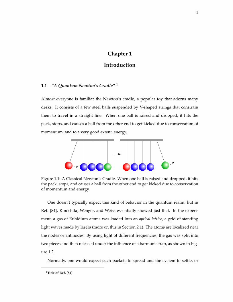
1.1 “A Quantum Newton’s Cradle” 1
Almost everyone is familiar the Newton’s cradle, a popular toy that adorns many
desks. It consists of a few steel balls suspended by V-shaped strings that constrain
them to travel in a straight line. When one ball is raised and dropped, it hits the
pack, stops, and causes a ball from the other end to get kicked due to conservation of
momentum, and to a very good extent, energy.
Figure 1.1: A Classical Newton’s Cradle. When one ball is raised and dropped, it hitsthe pack, stops, and causes a ball from the other end to get kicked due to conservationof momentum and energy.
One doesn’t typically expect this kind of behavior in the quantum realm, but in
Ref. [84], Kinoshita, Wenger, and Weiss essentially showed just that. In the experi-
ment, a gas of Rubidium atoms was loaded into an optical lattice, a grid of standing
light waves made by lasers (more on this in Section 2.1). The atoms are localized near
the nodes or antinodes. By using light of different frequencies, the gas was split into
two pieces and then released under the influence of a harmonic trap, as shown in Fig-
ure 1.2.
Normally, one would expect such packets to spread and the system to settle, or
1Title of Ref. [84]

2
Figure 1.2: A Quantum Newton’s Cradle. The steel balls in the original toy are re-placed with wave packets made of hundreds of Rubidium atoms, and collide in thecenter. This is a schematic of what the experiment observes. Image provided by DavidWeiss.
equilibrate. However, they noticed that after several thousand collisions the system
still oscillated back and forth, and momenta didn’t reach an equilibrium distribution
at long time. Absorption images of the experiment taken at different times reveal this
oscillation (see Figure 1.3).
The strange behavior observed was ascribed to the so-called integrability of such a
one dimensional gas of neutral integer spin atoms2. The existence of several additional
conservation laws, a property of such models, was conjectured to be the reason for the
behavior; these conservation laws seemed to protect the system from decoherence and
mixing. Indeed this has been nearly conclusively established by numerous subsequent
experiments and theory. See Ref. [26] for a detailed account.
This experiment was a remarkable breakthrough on multiple fronts. First, the fact
that such a purely quantum phenomenon can be observed in a completely artificially
constructed experiment is remarkable, and speaks to the technological progress scien-
tists and engineers have made in the fields of laser optics, cold atoms, and imaging.
Second, the phenomenon itself is rather unexpected and new to the realm of quan-
tum dynamics, and the long life time of the system needs some explanation. Third, it
2We’ll have a lot more to say about integrability in the other chapters.

3
Figure 1.3: Absorption images of the gas clearly showing the two packets oscillatingback and forth. Image provided by David Weiss.
gives a tremendous boost to the study of nonequilibrium phenomena theoretically by
providing a trustworthy experimental basis to test theories. The progress since then
has been manifold. We’ll explore this in more detail in Chapter 2. For now, as an in-
dicator, Figure 1.4 shows the growth in the number of articles containing the words
“nonequilibrium” (and variations) and “quantum” in the abstract. The blue curve
tracks articles only on the cond-mat arXiv, while the red curve tracks all other physics
arXivs. Notwithstanding the rather incomplete nature of this plot, it still indicates that
nonequilibrium quantum phenomena have gained significant traction in recent years.

4
Figure 1.4: Trends in arXiv articles talking about quantum nonequilibrium physicsfrom 1993 to 2013. (2013 extrapolated to full year)
1.2 Quantum nonequilibrium physics
Experiments like the one described in the previous section, and many others 3 provide
not only the motivation to theoretically examine quantum nonequilibrium problems,
but also a context in which to study these phenomena. Before we move on I’ll describe
this context, namely that of quench dynamics.
1.2.1 What is a quench?
In this work, I focus on a specific way of throwing a system out of equilibrium called
a “quantum quench”. A quantum quench, like its metallurgical counterpart, involves
suddenly changing a parameter of the system. The quantum analogs of quenching
a hot piece of metal in cold water are for example, suddenly changing the size of
the system, changing an external electric or magnetic field, or changing a coupling
strength. In general, any sudden change affecting the system will be called a quench.
As we will see in Chapter 2, a lot of these protocols are achievable in experiments.
Theoretically, a quantum quench is usually modeled literally as a sudden change.
For instance, if the quench involves adding a term HI to the initial Hamiltonian H0 of
3See e.g., Refs. [20, 21, 29, 49, 102, 110, 120, 123, 135] for a collection of recent experiments and Refs. [17,18, 42] for reviews.
5
a system, then we quite literally write down the full Hamiltonian as
H = H0 + θ(t)HI (1.1)
where we use the standard Heaviside θ function. Experimentally, the word sudden
doesn’t mean anything and it becomes important to characterize what we mean by
“sudden”. Usually, this means that the time over which the quench occurs, τQ, is
much shorter than all other time scales in the system. In the experimental context,
this is usually the fastest relaxation time in the experiment, which is on the order of
milliseconds.
It is easy to see why a quantum quench is a good protocol to study nonequilibrium
dynamics. First, a system in or near equilibrium is in its ground state and possibly a
few low lying excited states. Such a system is characterized by a small finite number
of eigenstates which are nearby in energy. In a global quench however, we put a fi-
nite amount of energy density into the system, and potentially excite very high energy
states. More precisely, starting with an initial state |Ψ0〉, the quench evolves this with
a Hamiltonian H,
|Ψ(t)〉 = e−iHt|Ψ0〉 = ∑n
e−iEnt|n〉〈n|Ψ0〉, (1.2)
and the eigenstates (of the final Hamiltonian) that participate in the time evolution
depend only on the overlaps with the initial state. In general, an arbitrarily large
number of eigenstates participate, corresponding to arbitrarily large energies, only
determined by the initial state and the final Hamiltonian. The system is therefore far
from an equilibrium state. This can also be viewed as expanding a particular vector in
the Hilbert space of a quantum system in an arbitrary orthonormal basis. Naturally,
for a generic initial state, one expects a linear combination of a large number of vectors
from the new basis. The initial state clearly plays a very important role, and this will
be discussed in further detail. Eq. (1.2) also gives us an idea as to why calculating the
quench dynamics is a hard problem – it requires knowledge of the entire spectrum,
and the ability to carry out the summation over oscillating phases.
There are also other protocols for a quench. These aren’t sudden but proceed over
some finite amount of time and typically occur when a coupling constant or external

6
field is changed to drive the system through a phase transition. For example, in the
anisotropic Heisenberg chain, the anisotropy ∆ can be changed from less than one to
greater that one, driving the system from the gapless phase into the gapped phase.
Driving a system through a critical point at a steady rate is also considered a quench.
This is because as the parameter reaches its critical value, the relaxation time of the
system diverges, and any finite rate becomes a rapid quench. In other words, it is not
possible to maintain adiabaticity. This leads to the appearance of defects (domains of
different phases) and goes under the name of the Kibble-Zurek mechanism [27, 83,
145]. We do not study these quench protocols.
1.2.2 A note on “nonequilibrium”
Colloquially speaking, equilibrium usually refers to situations that are static in time
and nonequilibrium refers to situations that are changing in time, or dynamic 4. The
title of this dissertation then looks a little redundant, for either “dynamics” or “non-
equilibrium” should suffice to describe the situations we are interested in. I use non-
equilibrium dynamics to indicate that indeed these systems are away from any equi-
librium state but also fluctuate appreciably in time, as opposed to systems that are
away from their equilibrium state but slowly changing in time, or systems that are
indeed dynamic, for example, traveling waves, but are in a nonequilibrium steady state
in the sense that they are solutions of time-independent equations of motion. We are
interested in the entire gamut of nonequilibrium and dynamical processes, and steady
states are certainly part of that.
1.2.3 Integrable models
As mentioned earlier, integrable models have properties that makes their dynamics
different from generic models, mainly having to do with the presence of additional
conservation laws. In this work, we are primarily interested in the quench dynamics
of such models.
4Like more or less every scientifically rigorous statement, this one needs to be qualified with ifs andbuts, but these will become clearer as we go on, and I will avoid getting tied up here.

7
A rigorous definition of an integrable model is not essential here. Instead, I will
use a working definition. For our purposes an integrable model is one that can be
solved exactly using the Bethe ansatz. We’ll discuss the properties that a particular
model must have for integrability and we’ll describe integrability in more detail in
Chapter 3. For now, an integrable model is one for which we can explicitly write
down the multiparticle eigenstates. As far as this work is concerned, these are all one
dimensional models obtained from physical systems via some approximations and
simplifications, which will be discussed in detail in Chapter 3. As seen in Section 1.1,
these models describe certain experiments very well. To reiterate, integrable models
differ from nonintegrable ones in fundamental ways, and signatures of this can be seen
in experiments.
1.3 An overview of nonequilibrium phenomena
The success of thermodynamics as a broad framework to explain a wide array of equi-
librium phenomena ranging from the specific heat of solids to phase transitions, quan-
tum statistical properties via the partition function [127], and in general the notion
of statistical ensembles has led to equilibrium phenomena becoming the norm. It
is of course entirely the other way around — in nature we are surrounded by non-
equilibrium phenomena. The Earth’s motion around the Sun, the Moon’s motion
around the Earth, the flow of rivers and the periodic nature of tides are all dynam-
ical phenomena. It is therefore surprising that so many of these phenomena can be
described by a rather simple set of laws and equations. The fact that something as
dynamic as water becoming steam can be described in terms of a few numbers (the
critical exponents [92, 127]) is a remarkable consequence of what we now understand
as renormalization and the emergence of effective theories. The same framework can
be used to understand the ferromagnetic transition in some metals, a very different
physical system, but surprisingly the underlying effective theories look very similar.
Unfortunately, truly nonequilibrium phenomena have not been amenable to such
global laws, although a variety of methods have been developed to tackle different
8
types of nonequilibrium problems [38]. While notions of temperature and pressure
go back to the early 1600s, the foundations for a statistical or probabilistic treatment
of many particle systems began with Bernoulli and was further developed by Gibbs,
Boltzmann and others [75]. Bernoulli’s work on fluid dynamics can in fact be con-
sidered one of the earliest attempts at understanding the nonequilibrium problem
of fluid flow. However, early notions of nonequilibrium thermodynamics appeared
in the form of irreversible processes. The most successful formulation was the bal-
ance equation approach, which was essentially a flow equation for entropy that took
into account entropy production due to irreversibility in the system. The type of non-
equilibrium phenomenawe study are different in that in a quench, energy and entropy
are pumped into the system during the quench, but the system evolves unitarily, and
depending on the particular system at hand can be invariant under time reversal. It
is only systems connected to external baths that see continuous entropy production in
our context. This is for example required to sustain a current through the system.
Several natural phenomena are dynamical in nature. Weather systems, traffic pat-
terns, the flow of rivers, the responses of a bridge to people walking and wind, the
continuous effect of tides on a shoreline form a small subset of the macroscopic phe-
nomena that one would call dynamical. The time scales of the dynamics vary vastly
— some slow and some fast with respect to time scales of our observation of these
phenomena. A growing tree doesn’t seem to be doing much over what would be a
long time by our standards, but this is merely because what we observe is limited.
On a microscopic scale, one can argue that every system is dynamical. Some of
these systems do not deviate appreciably on a macroscopic scale from some equilib-
rium, and some do not deviate appreciable even microscopically. These are the types
of system that one would call equilibrium systems, and can be described by the laws
of thermodynamics and certain emergent macroscopic observables. A gas in a con-
tainer for example can be described by its pressure, volume, and temperature to a very
good approximation, and even though the microscopic description is dynamic and the
gas particles are in continuous motion, collision, and vibration, the three macroscopic
quantities do not vary appreciably. This quasi-equilibrium behavior of systems is due

9
in part to them being in an environment, the so-called thermodynamic bath, and any
coherent nonequilibrium behavior is rapidly quelled by dephasing of states due to
interaction with the environment and dissipation of energy.
The one nonequilibrium phenomenon that is commonplace is the existence of cur-
rents. If we connect a piece of resistive wire like a light bulb to a battery, then the
potential difference drives a steady current through the bulb, until all the charge of the
battery equilibrates, i.e., the battery discharges. The nonequilibrium phenomenon in
question here is a steady state produced by a bias in the boundary conditions. It is sim-
ilar to a ball rolling down an inclined plane. The steady state phenomenon occurs after
any transients have died out, and overcomes dissipation since energy is continuously
pumped into the system by maintaining a potential energy bias.
Steady state currents are a staple of transport problems in several quantummodels,
e.g. quantum hall states [70], transport through impurities [46, 47, 100], and currents
in one dimensional wires. This area has also attracted a lot of attention lately with the
technological advances in fabricating quantum dots and controlling tunneling barriers
and quantum point contacts [54]. It is also possible to establish currents in a quench
experiment, as we will describe in Chapter. 6. Recently transport has been experi-
mentally observed in the ultracold atom context [101, 30]. Steady state currents in the
Andersonmodel, that shows the Kondo effect [68] is currently a theoretically unsolved
problem in spite of the model being integrable. The two lead model, necessary to es-
tablish a current poses complications due to the so-called string states and has eluded
a fully exact treatment [28].
1.4 Outline of the thesis
The remainder of the thesis is organized as follows.
In Chapter 2 I discuss some features of quench dynamics in closed one-dimensional
systems. I then describe the specific experimental and theoretical motivation to study
non-equilibrium phenomena. In Section 2.1, I focus on the specific experiments that
are of relevance in the context of this work. I will describe what models can be used to

10
describe these experiments, and the different phenomena that have been observed. In
Section 2.2, I describe the commonly used tools to study non-equilibrium phenomena,
their advantages and disadvantages, and provide reasons as to why new tools are
required for a complete understanding on such phenomena. In Section 2.4, I survey
some of the literature in the field, and describe some of the major results. Section 2.5
provides an overview of the open questions in the field, and also describe which of
these questions, the present work addresses.
In Chapter 3, I provide a brief review of integrability and the Bethe Ansatz (Sec-
tions 3.1 and 3.2). Specifically, I describe only those aspects of the Bethe Ansatz that
are useful for the purposes of this work. In Section 3.3, I show some examples of how
the Bethe Ansatz can be used to obtain eigenstates of models that we will study the
dynamics of. In Section 3.4, I discuss the role of the Bethe Ansatz in the context of
quantum quenches, the advantages, and the difficulties involved in a direct applica-
tion to dynamics.
Carrying on along these lines, in Chapter 4 I review Yudson’s integral representa-
tion for arbitrary states in an infinite volume system. I also derive the completeness
of the “Yudson” basis for a specific case. In Section 4.3 I provide an explicit example
of how the Yudson integral representation can be used to obtain the quench dynamics
using the Resonant Level Model. I will derive finite time behavior and asymptotics.
Section 4.4 describes how the Yudson representation can be extended to other inte-
grable models, what the challenges are, and how we can perhaps overcome them.
Chapters 5 and 6 form the main body of this work. I derive the Yudson representa-
tion for the Lieb-Liniger model and the Heisenberg chain, and use it to study the time
evolution of these two models. In the Lieb-Liniger case, we show how the dynamics is
controlled by fixed points at long time that either lead to fermionization of the bosons,
or formation of bound state correlations. Chapter 6 presents ongoing research.
In Chapters 7 and 8 I present possible future directions of this work, and provide a
summary and conclusion to the thesis.

11
Chapter 2
Quantum nonequilibrium dynamics
Quench experiments have come to the forefront of studies in quantum nonequilibrium
phenomena due to tremendous technological progress over the last decade or so. Be-
fore we venture into a theoretical description of specific quenches in specific systems,
it is necessary to provide the experimental context in which this work is based, namely
that of ultracold atoms. I will also briefly introduce the various theoretical models and
approaches to understanding these phenomena.
2.1 Experiments to probe out of equilibrium phenomena
2.1.1 Experiments with cold atoms
The first big success of cold atoms takes us to the 2001 Physics Nobel prize awarded
to Cornell, Ketterle, and Wiemann “for the achievement of Bose-Einstein condensation in
dilute gases of alkali atoms, and for early fundamental studies of the properties of the conden-
sates” [105] for work done in 1995 [34, 76, 37]. They for the first time explicitly showed
a gas of bosons (Sodium atoms) forming a condensate, a prediction made by Bose
and Einstein in the mid-twenties [19, 41]1. In these experiments, a gas of Rubidium
or Sodium atoms was trapped and cooled using lasers leading to the formation of a
condensate. Figure 2.1 shows a photograph of a trapped cold gas.
Fast-forward about 18 years, andwe have the state-of-the-art experiments in which
bosonic and fermionic gases can be trapped and cooled, their interactions can be con-
trolled, and phase transitions can be driven by applying external electric andmagnetic
1Superfluidity, essentially a condensation phenomenon, was observed in the late 30s but it was neverobserved in a gas before this.

12
Figure 2.1: A trapped gas of Sodium atoms confined by lasers. Reproduced fromRef. [67].
fields [18, 17, 42, 31, 93]. Recently thermal transport has also been observed in cold
atoms [20].
It is this control and precision that has made ultracold atoms a perfect setting for
the study of isolated quantum systems. Most of the theoretical studies about the out
of equilibrium behavior, especially quench dynamics is in the context of cold atom
experiments, and it is indeed the experimental arena to which our calculations apply.
The systems are formed by trapping a gas of atoms using standing light waves made
by lasers. The gases are cooled evaporatively and are well isolated from any thermal
baths making them ideal for studying relaxation and thermalization in isolated quan-
tum systems. The interactions between the particles, the potentials, and their statistics
can be controlled by the use of external magnetic and electric fields, tuning the opti-
cal lattice, and loading different atoms into the traps. Systems with mobile impurities
can also be studied by loading two or more different species of atoms into the lattices.
Lattices can be three dimensional or can be made quasi-1d or 2d by using confining
potentials. The typical relaxation and evaporation time scales in these systems are in

13
the milliseconds. This makes measurement easier than in solid state systems. It also
allows for sudden quenches. Disorder is also largely absent, unless introduced.
Tuning the parameters allows the study of superfluid behavior, Mott insulators,
spin chains and so on. Such a gas trapped by lasers and cooled to nano-Kelvin tem-
peratures can be quenched by suddenly changing the interaction between the atoms,
and the external trapping potential. Evolution can be globally observed by imaging
the gas, and the time evolution of densities and correlation functions can be obtained
from these images [18, 57, 84, 102].
In one dimension, which is of particular interested to us, the typical models that are
used to study these systems are the Bose-Hubbard model, the XXZ model, the Sine-
Gordon model and the Lieb-Liniger model. Each of these models studies a different
regime of the gas. The Bose-Hubbard model is optimal for atoms hopping on a one
dimensional lattice. A particular limit of the Bose-Hubbard model can be mapped to
the XXZ spin chain [8] which is integrable. The continuum gas is captured by the
Lieb-Liniger model.
We are primarily concerned with integrable models. In this context, it is an im-
portant question as to how “integrable” a particular experimental realization is. Often
the experimental setup maintains an external trapping potential and including such
a potential in an integrable Hamiltonian may render the system non-integrable. Ex-
perimentally, such potentials need to be eliminated to the extent possible. This can be
partially achieved by using a flat potential profile and concentrating on the center of
the trap. As has been shown in Ref. [84], and discussed in Section. 1.1, the dynamics in
certain experiments very closely resembles what we expect from an integrable model,
and it is believed that we can indeed create integrable systems to a close approxima-
tion. This also opens up the question of how far from integrability do we need to be in
order to see the effects of integrability breaking.
2.1.2 Optical lattices
Optical lattices form the basis of trapping ultracold atoms in various configurations
(see Refs. [16, 73] for reviews). The concept is simple. As shown in Figure 2.2, an

14
optical lattice consists of opposing laser beams. In one dimension, two opposing co-
herent laser beams whose phases are appropriately tuned can set up a standing wave.
The electric field interacts with the induced atomic dipoles creating a potential for the
atoms,
Vdipole = −d · E(r) ∼ αI (2.1)
where α is the frequency dependent polarizability and I is the intensity of light. By
tuning the frequency away from any atomic resonances, atomic transitions and en-
ergy transfer are avoided. By tuning the frequency to be greater than or less than the
resonance frequency, an attractive or repulsive potential can be obtained depending
on the sign of the detuning. Laser light of wavelength λ produces standing waves hav-
ing λ/2 periodicity – this sets the lattice constant. Three laser beams in perpendicular
directions can trap atoms in all three directions and make a 3d lattice.
Figure 2.2: An optical lattice formed by standing waves of laser light. The frequenciescan be tuned to localize the atoms at the nodes or antinodes.
Atoms localized in potential wells formed by the optical lattice can tunnel into
neighboring wells, and the tunneling rate determines the hopping probability in a
tight-binding type of Hamiltonian, and is proportional to the height of the well and

15
consequently the intensity of the laser.
t ∝ V0 ∝ I. (2.2)
By increasing the intensity, we can strongly localize the atoms, creating an insulator,
or lower it creating a fluid.
On top of the underlying lattice that localizes the atoms, additional laser profiles
can create traps of various shapes, a typical one being parabolic. These traps can also
be used inmaking a three dimensional gas quasi-2d or quasi-1d bymaking the traps in
some directions very steep so that the kinetic energy is suppressed in those directions.
Once atoms are loaded into an optical lattice and cooled, we are ready to turn on
interactions, let the gas expand, and make measurements!
2.1.3 Feshbach resonances
The tunability of the interactions between ultracold atoms is a very useful feature as it
can be used to realize several different regimes of behavior like Bose-Einstein conden-
sate (BECs), superfluidity, Mott insulators, and so on [16, 110, 73, 59]. In the approx-
imation that the only important interactions between the atoms are two-body s-wave
interactions (as assumption that is usually valid in ultracold atoms [31]), the inter-
action potential, or coupling strength depends only on the corresponding scattering
length,
V =4πh2a
m(2.3)
where m is the atomic mass, and a is the s-wave scattering length. This scattering
length can be varied from −∞ < a < ∞ by exploiting the so-called Feschbach reso-
nance, which is essentially a resonance between a bound state and a scattering state.
A positive binding energy leads to a repulsive interaction, while a negative binding
energy leads to an attractive interation. The position of the resonance, and therefore
the binding energy can be tuned using an external magnetic field.
The spin structure of the atoms play a crucial role in Feshbach resonances. The
three spins involved are the electron spin, the orbital angular momentum, and the
nuclear spin. For the alkali metal atoms like 7Li typically used in ultracold setups,

16
the ground states are usually zero orbital angular momentum states. The only rele-
vant quantum numbers then are the nuclear spin and its projection, and the electron
spin, which is always 1/2. The atom then behaves as a fermion or boson depending on
the nuclear spin quantum number. States corresponding to different nuclear spin can
further be split by an external magnetic field. In a collision of two atoms, several of
these can be accessed – the potentials corresponding to different states are called colli-
sion channels. The interaction between two collision channels can produce a Feshbach
resonance, described below.
Consider the simple case of two atoms interacting via the potentials shown in Fig-
ure 2.3. The two potentials usually correspond to different hyperfine states split by
Figure 2.3: Two channels for interatomic potentials. Reproduced from Ref. [31].
an external magnetic field. At large distance R, the atoms are essentially free. When
they come close however, if the bound state energy of the closed channel is similar to
the scattering energy, then a resonance occurs. The scattering length corresponding to
this resonance depends on the splitting between the two states, and can be controlled
by changing the external magnetic field,
a(B) = a0
(
1− ∆
B− B0
)
. (2.4)
In the above equation, a0 is the scattering length off-resonance associated with the
background potential of Figure 2.3. B0 is the resonant value of magnetic field, which
is a property of the particular species used and the particular hyperfine state involved
in the resonance, and ∆ is the width of the resonance. Figure 2.4 shows a plot of the

17
scattering length as a function of the magnetic field.
-3 -2 -1 1 2 3
B-B0
D
-4
-2
2
4aBa0
Figure 2.4: Scattering length as a function of magnetic field near a Feshbach resonance.The scattering length can be made positive or negative, corresponding to repulsive orattractive interactions.
The scattering length has a divergence and a discontinuity B = B0; on either side
of this divergence the sign of the scattering length is different. Tuning the resonance
through this allows us to go from repulsive to attractive interactions and vice versa.
There also exists a zero crossing, or a point where the scattering length goes to zero. It
is easy to see that this point is
B = B0 + ∆. (2.5)
At this point, the particles become noninteracting.
2.1.4 Recent developments
Over the last decade, the use of the Feshbach resonance to establish fine control over
ultracold gases has become commonplace [31]. Recently more exotic properties are
being realized [17], as ultracold gases slowly achieve the ideal of Feynman’s quantum
simulator [48].
Artificial gauge fields and topological properties
The atoms used in ultracold experiments are neutral and we cannot examine their
interaction with electric or magnetic fields in order to understand the behavior of

18
charged particles. In particular, producing the quantum Hall effect seems impossi-
ble. The physics of the quantum Hall effect is a simple example of so called topologi-
cal properties. The Hall conductance is quantized, and the quantization filling factor
corresponds to the Chern number, the coefficient of a total derivative term in the La-
grangian. Vorticity in a superfluid is also such a topological property emerging from
the boundaries or a singularity in the flow, and as such is a global phenomenon.
One ingenious method of simulating vorticity or a Lorentz force in an ultracold
atom experiment is to rotate the gas maintaining a balance between centrifugal and
trapping potentials. The Coriolis force then provides the “Lorentz force” since it has
the same velocity dependence and form,
FCoriolis = −2mΩ × v, FLorentz = −qB× v. (2.6)
The mass m plays the role of the charge q, and the angular velocity Ω plays the role of
the magnetic field B.
There are also other optical means of producing vorticity. See Ref. [17] for a review
and the references therein for details.
Atom scale imaging
Absorption imaging is the common way in which a gas of ultracold atoms is mea-
sured. Near resonant light is shone on the sample, regions of high density absorb and
scatter more light and regions of low density, less. The resulting image is captured on
a Charge Couple Device (CCD) sensor, similar to the ones in digital cameras, albeit
through microscope lenses. This however does not provide atom scale resolution.
Recently, fluorescence imaging with high resolution low noise CCDs has made
it possible to resolve single atoms by maintaining a very low intensity of fluores-
cence [17] – each atom scatters only a few thousand photons. Further, the gas can
be imaged at any point by freezing it momentarily by increasing the lattice depth to
prevent tunneling. The primary difference is that in absorption imaging, the scattered
light is lost, and only the “shadow” is recorded. However, in fluorescence imaging

19
each atoms displays its presence via fluorescence from resonant light. This new tech-
nique allows in-situ atom resolved measurements.
2.2 Theoretical methods and tools
In Physics, experiments are always modeled, and one aims to provide the simplest
possible model that explains the findings of the experiment, and perhaps more 2. In
the field of nonequilibrium quantum dynamics, experiments using ultracold atoms
have turned out to be unusually clean (i.e. disorder free) and well controlled, and are
proving to be an alternate means of understanding the physics. Instead of studying
a model, one simulates it, but this time with a real quantum system, as opposed to a
simulation on a classical computer, implementing a point of view going back to Feyn-
man [48]. However, whereas making measurements on an experiment in various dif-
ferent conditions gives us tremendous insight, predicting new behavior or developing
a broader understanding requires models, and we need theoretical tools to calculate
the predictions of these models.
The cold atom experiments that we are interested in are on one dimensional sys-
tems of bosons or fermions. There are a few effective models that can be used to
understand different regimes of the gas.
2.2.1 Models
The most basic model describing these experiments is the Hubbard model,
HHubbard = t∑〈ij〉
c†i cj +U(c†j cj)2, (2.7)
which describes either bosons or fermions hoping between nearest neighbors on a
lattice with on-site interactions. Additional terms can be included to account for next-
nearest-neighbor hopping, longer range interactions, and external potentials. Various
limits of the couplingsU/t lead to different effective models. By changing lattice para-
meters or considering excitations on top of the lattice, a further set of effective models
2Occams razor

20
can be realized.
For instance, for bosons in the regime where U/t ≫ 1, double occupancy is sup-
pressed, andwe get amodel of hard core bosons hopping on a lattice. A Jordan-Wigner
transformation [52] can be used to transform the bosons to free fermions. It essen-
tially maps the bosonic creation operators to fermionic creation operators. However,
in order to get the commutation relations correct (bosons commute, while fermions
anticommute), the mapping is a little more complicated:
b†j = eiπ ∑i<j c†i cic†j ,
bj = cje−iπ ∑i<j c
†i ci ,
b†j bj = c†j cj.
(2.8)
A similar transformation can be used to go between spin-1/2 operators and fermions in
one dimension, and therefore this model can also be mapped to the interacting XXZ
model,
HXXZ = −J ∑j
σxj σx
j+1 + σyj σ
yj+1 − ∆(σz
j σzj+1 − 1) (2.9)
Chapter 6 presents some preliminary work on the dynamics of the critical (isotropic,
∆ = 1) Heisenberg model.
The “lattice” is usually formed by a deep laser standing wave which localizes the
atoms at the nodes or antinodes. First, the lattice spacing can be controlled by using
different laser frequencies, and the depth can be controlled by varying the amplitude.
Making the amplitude small allows the atoms to tunnel easily, transitioning to a con-
tinuum model of free bosons, or with δ-function interaction, the Lieb-Liniger model,
described in Chapters 3 and 5. The intermediate regime between the lattice and the
continuum can be captured by adding a sinusoidally varying potential to a continuum
bosonic model, giving us the sine-Gordon model.
Of the above models, all other than the Bose-Hubbard model are integrable and
can be solved exactly. Such models are of special interest to us. It is indeed remarkable
that such specialized models can be experimentally realized. We do however, neglect
three body losses and next-nearest-neighbor (NNN) hopping or long range interac-
tions. These processes typically render models nonintegrable and one typically needs

21
numerical techniques to study them. Fortunately, neglecting these is a reasonable as-
sumption in cold atom experiments.
Inspite of these simplifications, the quench dynamics of these models is not easy
to compute. As explained in Section 2.3, a quench potentially excites arbitrarily high
energy eigenstates of the final (i.e., post-quench) Hamiltonian. Most theoretical tools
are designed to deal with either ground state properties and small excitations above
the ground state, or to study the effect of interactions perturbatively, and especially to
deal with equilibrium situations. We need a more general set of tools, and some new
ones to deal with the far from equilibrium, highly excited, and strongly interacting
systems in quench experiments. This is especially true of one dimensional systems,
which is the subject of this thesis. In one dimension, due to geometric hindrance, in-
teractions are always strong. The best example of this is that the Fermi liquid breaks
down in one dimension and we are forced to use a more complicated picture, namely
the Luttinger liquid. Fortunately the Luttinger liquid is exactly solvable via bosoniza-
tion, and indeed displays physics that is unique to one dimension, namely spin-charge
separation, the idea that the spin and charge degrees of freedom propagate at different
velocities. See Ref. [52] for more on the various methods to solve the Luttinger liquid.
2.2.2 Field theoretic methods
Renormalization group based methods have been tremendously useful in all of con-
densed matter physics in understanding low energy effective theories of a variety of
phenomena [5]. Out of equilibrium, the standard technology of calculating expecta-
tion values fails, and one has to employ the Schwinger-Keldysh formalism [128, 82].
See Ref. [4] for a review.
In order to apply perturbative techniques the model must have a small parameter.
Usually the coupling constant of the interaction terms are treated as small, i.e., weak.
Basically, the perturbation around the solvable model must be small. It is for example
possible to perturb in an external electric field, when the model without the electric
field is exactly solvable. A series expansion can then be developed in the external field,
and time dependent expectation values can be evaluated as a series. This is especially
22
useful when the question of interest is the linear response of a system [108, 107]. In
other cases it is possible to develop a perturbation series in the inverse number of
flavors or colors (internal symmetries), the so-called large-N limit. These expansions
are exact in all orders of the appropriately scaled coupling constant but approximate
in 1/N [115].
2.2.3 Numerical methods
With the development of powerful algorithms and fast computers, it has become fea-
sible to study the dynamics of quantum systems purely numerically. There are several
commonly used techniques that each have their advantages and disadvantages. Some
numerical methods aim to exactly solve a given system, while others use various ap-
proximations. Methods like exact diagonalization, Density Matrix Renormalization Group
(DMRG),Dynamical Mean Field Theory (DMFT),Numerical Renormalization Group (NRG)
have been implemented numerically. I will briefly describe two of these that have been
the most popular with the field of nonequilibrium quantum dynamics.
Exact diagonalization
The method is precisely that. Given a Hamiltonian, one solves the matrix eigenvalue
problem. For this to be feasible, the volume of the system is a fixed finite number, say
L, and the number of particles is fixed as well, say N. One can then write down a basis
for the Hilbert space, and in this basis, the Hamiltonian is a matrix. This matrix is
then diagonalized, giving the eigenvectors and eigenvalues. If only the ground state
properties and perhaps a few excitations are desired, the task is computationally a
little simpler. However, in order to calculate time evolution after a quench, where all
the eigenstates that have a nonzero overlap with the initial state are relevant, one has
to carry out a full diagonalization.
Full diagonalization algorithms are computationally intensive and it is not feasibly
to study very large systems. Sizes of L ∼ 20 are about as large as possible [126].
Sometimes it is possible to decrease the effective size of the Hilbert space by exploiting
23
other conserved quantities. For instance, a spin model with N spins has a Hilbert
space dimension of 2N . However, if the model conserves either the total spin or Sz,
then one can work in a particular spin sector with a fixed Sz. If out of the N spins,
M are up and N − M are down, then the z-component of the spin is fixed at Sz =
1/2(2M− N), and the dimension of the Hilbert space is now (NM). As an example, for
N = 20, without restricting to the spin sector, the dimension is 220 106. For N = 20 and
M = 10, we instead have a Hilbert space dimension of about 105, nearly a factor of 10
improvement. It also makes more physical sense to treat each spin sector separately if
there is no mixing.
The advantage of exact numerical diagonalization is that once the eigenvalue equa-
tion is solved, we can extract anything we want. Expectation values of operators in
arbitrary states, time evolution, entropy calculation, correlation functions are all eas-
ily accessible once the entire spectrum is known. See Refs. [116, 117, 118, 65, 119] for
example.
Density Matrix Renormalization Group
The Density Matrix Renormalization Group (DMRG) [137, 36] has become a very pop-
ular method recently because of its versatility and ease of application to a wide variety
of one dimensional models, and initial states. In its equilibrium avatar, the method
can effectively find the ground state of a system without having to diagonalize the
full Hamiltonian, a problem that is exponential in the size of the system, due to the
way the Hilbert space of quantum problems scales. The DMRG method overcomes
this by using representative states to start with, and improving the guess for the true
ground state iteratively, each step involving a much less accurate diagonalization of
the Hamiltonian to find the lowest energy states. Further, in each step, only a subset
of the system can be considered, thus speeding up the process.
This method can be extended to calculate time dependence by using some approx-
imation of the time evolution operator, and directly acting on an initial state. The
main speed up is obtained by using a suitably truncated Hilbert space instead of the
full Hilbert space. As the entanglement increases with time evolution, more and more

24
states in the exponentially large Hilbert space need to be retained, and therefore even-
tually the method slows down to impractical speeds. Further, it is not straightforward
to use this method on models with long range interactions. See [63, 125, 126] for re-
views.
2.2.4 Exact methods
These methods are applicable to a specific set of models. They allows the exact calcu-
lation of correlation functions, ground state properties etc. Exact in this context means
that we either have an analytical result, or a set of integral or differential (or both)
equations whose numerical solution provides us with the numbers. It is different from
exact diagonalization, since that method, while also being exact within numerical error,
applies to direct numerical solution of the Schrodinger equation, and is restricted to
finite sized lattice models.
In this Section, we will outline the three most commonly used exact methods, and
they all apply to models in one spatial (and one time) dimension.
Conformal field theory
Conformal Field Theories are a class of field theories that have no length scale (are
scale invariant), and typically describe critical points. The field theory describing the
critical point is an effective field theory, constructed from the quasi-particle excitations
of the critical point [144]. The key aspect here is that conformal invariance (Lorentz
invariance plus scale invariance plus inversion symmetry) in one dimension strongly
constrains all correlation functions to a fixed form determined by the field content of
the theory. For more details, see Refs. [144, 51]
Conformal field theory methods have been successfully employed to understand
nonequilibrium problems, such as the steady state current through quantum point
contacts [47, 46], in quantum hall systems [70] and Ising models [23].

25
Bosonization
Bosonization is a method where collective excitations in fermion densities are treated
as the quasi-particle. The resulting effective field theory contains bosonic fields, and
four-point local interactions in the fermions are reduced to two-point interactions,
thus making them quadratic. This transformation renders, for example, the Luttinger
liquid, which is interacting in the fermions, into a free field theory in terms of the
bosons [52]. On can also bosonize more complicated fermionic models to effective
interacting bosonic models, sometimes with topological terms. Ref. [98] provides an
excellent introduction to bosonization and the connection with Conformal Field The-
ory.
Bosonization is similar to othermethods like Jordan-Wigner transformationswhere
an appropriate field transformation (possible nonlocal) provides a more convenient
representation of the model. All these methods are more conducive to treating initial
states which are eigenstates of the model, and quenching the coupling constant. Start-
ing with a physical initial state in fermions and diagonalizing the model in terms of
bosons requires one to represent the initial state in an appropriate language, and this
is not always straightforward. The fermionic representation of hardcore bosons is one
such example [32, 33, 87].
Bethe Ansatz
The Bethe Ansatz is yet another technique that is applicable to a subset of models
that are defined as being integrable. Since this thesis primarily deals with integrable
models, a detailed exposition on the Bethe Ansatz as applicable here is provided in
Chapter 3.
2.3 Dynamics of 1d isolated many-body systems
While studying the thermodynamic properties of a quantum system, one needs to enu-
merate and classify the eigenstates of the Hamiltonian in order to construct the parti-
tion function. To achieve this, some finite volume boundary conditions are typically

26
imposed — either periodic boundary conditions to maintain translation invariance or
hardwall boundary conditions when the system has physical ends. One can then iden-
tify the ground state and the low lying excitations that dominate the low-temperature
physics. In the thermodynamic limit N→∞L→∞
≡ ρ, the limit of very large systems with large
number of particles at finite density, the effect of the boundary condition is negligible
and we expect the results to be universally valid.
When the system is out of equilibrium, a different set of issues arises. We shall
consider here the process of a “quantum quench”where one studies the time evolution
of a system after a sudden change in the parameters of the Hamiltonian governing the
system. To be precise, one assumes that the system starts in some stationary state
|Ψ0〉. This stationary state can be thought of as the ground state of some (interacting)
Hamiltonian H0. Following the quench at t = 0, the system evolves in time under
the influence of a new Hamiltonian H which may differ from H0 in many ways. One
may add an interaction, change an interaction coupling constant, apply or remove
an external potential or increase the size of the system. Further, the quench can be
sudden, i.e., over a time window much shorter than other time scales in the system,
driven at a constant rate or with a time dependent ramp.
In this paper we shall concentrate on sudden quenches where the initial state |Ψ0〉describes a system in a finite region of space with a particular density profile: lattice-
like, or condensate-like (see Fig. 2.5). Under the effect of the quenched Hamiltonian
the system evolves as |Ψ0, t〉 = e−iHt|Ψ0〉.
To compute the evolution, it is convenient to expand the initial state in the eigen-
basis of the evolution Hamiltonian,
|Ψ0〉 = ∑n
Cn|n〉, (2.10)
where |n〉 are the eigenstates of H and Cn = 〈n|Ψ0〉 are the overlaps with the initial
state, determining the weights with which different eigenstates contribute to the time
evolution:
|Ψ0, t〉 = ∑n
e−iǫntCn|n〉. (2.11)

27
(a)
(b)
σ
a
L
ρ ∼ NL
ρ ∼ Nσe−
x2
σ2
Figure 2.5: Initial states. (a) For aσ ≫ 1, we have a lattice like state, |Ψlatt〉. (b) For
a = 0, we have a condensate like state |Ψcond〉, σ determines the spread.
The evolution of observables is then given by,
〈O(t)〉Ψ0= 〈Ψ0, t|O|Ψ0, t〉
= ∑n,m
e−i(ǫm−ǫn)tC∗n Cm〈n|O|m〉,
(2.12)
with observables that may be local operators, correlation functions, currents or global
quantities such as entanglements.
The time evolution is characterized by the energy of the initial state,
ǫquench = 〈Ψ0|H|Ψ0〉 = ∑n
ǫn|Cn|2 (2.13)
which is conserved throughout the evolution, specifying the energy surface on which
the system moves. This surface is determined by the initial state through the overlaps
Cn. Unlike the situation in thermodynamics where the ground state and low-lying
excitations play a central role, this is not the case out-of-equilibrium. A quench puts
energy into the system which the isolated system cannot dissipate and it cannot relax
to its ground state. Rather, the eigenstates that contribute to the dynamics depend
strongly on the initial state via the overlaps Cn (see Fig. 2.6).
A vivid illustration comes from comparing quenches in systems that differ in the
sign of the interaction. In the Bose-Hubbard model and the XXZ model it has been
observed that the sign of the interaction plays no role in the quench dynamics [89, 8],
even though the ground states that correspond to the different signs are very differ-
ent. For example, for the XXZ magnet, the ground state is either ferromagnetic or

28
Neel ordered (RVB in 1d) depending on the sign of the anisotropy ∆. In Appendix A,
we show results for the Bose-Hubbard model, and provide an argument for this ob-
servation. The Lieb-Liniger model, whose quench dynamics we describe here, on the
other hand shows very different behavior, reaching an long time equilibrium state that
depends mainly on the sign of the interaction.
Figure 2.6: Difference between quench dynamics and thermodynamics. After aquench, the system probes high energy states and does not necessarily relax to theground state. In thermodynamics, we minimize the energy (or free energy) of a sys-tem and probe the region near the ground state.
In the experiments that we seek to describe, a system of N bosons is initially con-
fined to a region of space of size L and then allowed to evolve on the infinite line
while interacting with short range interactions. It is important to first understand
the time-scales of the phenomena that we are studying. There are two main types of
time scales here. One is determined by the initial condition (spatial extent, overlap
of nearby wave-functions), and the other by the parameters of the quenched system
(mass, interaction strength).
For an extended system, i.e., where we start with a locally uniform density (see
Fig. 2.5a), we expect the dynamics to be in the constant density regime as long as
t ≪ Lv , v being the characteristic velocity of propagation. Although the low energy
thermodynamics of a constant density Bose gas can be described by a Luttinger liq-
uid [52], we expect the collective excitations of the quenched system to behave as a
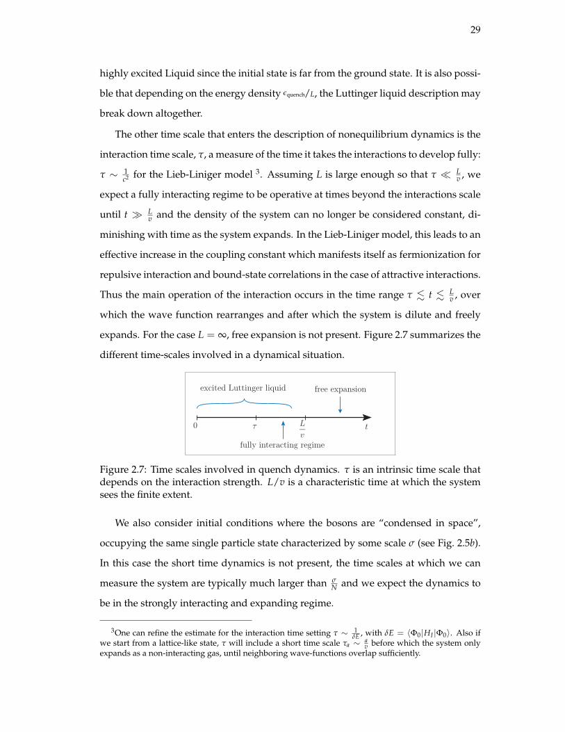
29
highly excited Liquid since the initial state is far from the ground state. It is also possi-
ble that depending on the energy density ǫquench/L, the Luttinger liquid description may
break down altogether.
The other time scale that enters the description of nonequilibrium dynamics is the
interaction time scale, τ, a measure of the time it takes the interactions to develop fully:
τ ∼ 1c2
for the Lieb-Liniger model 3. Assuming L is large enough so that τ ≪ Lv , we
expect a fully interacting regime to be operative at times beyond the interactions scale
until t ≫ Lv and the density of the system can no longer be considered constant, di-
minishing with time as the system expands. In the Lieb-Liniger model, this leads to an
effective increase in the coupling constant which manifests itself as fermionization for
repulsive interaction and bound-state correlations in the case of attractive interactions.
Thus the main operation of the interaction occurs in the time range τ . t . Lv , over
which the wave function rearranges and after which the system is dilute and freely
expands. For the case L = ∞, free expansion is not present. Figure 2.7 summarizes the
different time-scales involved in a dynamical situation.
t0 L
vτ
excited Luttinger liquid free expansion
fully interacting regime
Figure 2.7: Time scales involved in quench dynamics. τ is an intrinsic time scale thatdepends on the interaction strength. L/v is a characteristic time at which the systemsees the finite extent.
We also consider initial conditions where the bosons are “condensed in space”,
occupying the same single particle state characterized by some scale σ (see Fig. 2.5b).
In this case the short time dynamics is not present, the time scales at which we can
measure the system are typically much larger than σN and we expect the dynamics to
be in the strongly interacting and expanding regime.
3One can refine the estimate for the interaction time setting τ ∼ 1δE , with δE = 〈Φ0|HI |Φ0〉. Also if
we start from a lattice-like state, τ will include a short time scale τa ∼ av before which the system only
expands as a non-interacting gas, until neighboring wave-functions overlap sufficiently.
30
2.4 Established results
2.4.1 Eigenstate thermalization
An isolated quantum system evolves unitarily and a priori there is no reason why the
long time behavior should be independent of the initial states. In other words there is
no reason why the system should thermalize, and indeed we have seen examples of
integrable models that do not. However, for systems that do, we need to understand
possible mechanisms by which this can occur. The time evolution of an observable Oin a state |Ψ0〉is given by
〈O(t)〉 = ∑m,n
Omnc∗mcne
−i(En−Em)t (2.14)
where the cm are as usual the overlaps of the eigenstates of the Hamiltonian and the
initial state. If t → ∞ limit exists, then it must correspond to Em = En4. In the absence
of degeneracies, this gives
〈O(t)〉 = ∑m
Omm|cm|2 (2.15)
which is an average in the so-called diagonal ensemble.
Deutsch and Srednicki proposed a mechanism by which the expectation value of
the operator O(t) thermalizes at long time, i.e., reaches a value independent of the
particular initial state [39, 130]. Rigol et al propose a couple of other mechanisms for
the thermalization [117]. Together they amount to the following:
1. For physical initial state, the overlaps cn have a flat distribution and so we reach
themicrocanonical distribution obtained by assuming a priori equal probabilities;
2. The fluctuations in the operator matrix elements and the overlaps from one
eigenstate to the next are uncorrelated, so the sum is essentially an unbiased
sampling;
3. The operator matrix elements have a flat distribution, and factor out of the sum.
4While fairly intuitive, this statement is rigorous and a result of the Riemann-Lebesgue lemma [58].

31
Each of these scenarios can be realized, but it is not obvious that all thermalization
necessarily occurs in this fashion. Further, as we see in the following section, depen-
dence on the initial state can be partial.
2.4.2 Generalized Gibbs Ensemble
The idea of a thermodynamic ensemble goes back to Boltzmann and Gibbs, and the
roots lie in the probabilistic or phase space approach to the equilibrium configuration
of a gas. The basic notion is that the system maximizes the number of configurations
available for a particular macroscopic state. For a microcanonical description, this is
rule is satisfied by having equal a priori probabilities for the different configurations.
The quantity being maximized is the phase space volume, or the log of it, which up to
a factor is the entropy. The true power of this approach comes when the same notion
of maximizing entropy is taken to describe a system connected to a bath, giving us the
so-called canonical ensemble or Gibbs ensemble.
The notion of a Generalized Gibbs Ensemble goes back to Jaynes [74, 75] who
treated the Gibbs ensemble (or the canonical ensemble) as the simple outcome of max-
imizing the entropy of a system subject to constraints. The Gibbs ensemble is obtained
by requiring that the expectation value of the energy is fixed by the thermodynamic
bath,
ρGibbs =e−βH
Tr e−βH. (2.16)
The Lagrange multiplier for this constraint is β, the inverse temperature. It was a
natural extension to him that if the system has multiple constraints, then each of these
constraints must be taken into account. Accounting for a chemical potential and a
fixed expectation for the particle number N leads to the Grand Canonical Ensemble,
ρGC =e−βH−µN
Tr e−βH−µN. (2.17)
For a system with several constraints that can be written as expectation values of ob-
servables (or in general operators), the entropymust memaximized subject to all these
constraints giving
ρGGE =e∑j λj Ij
Tr e∑j λj Ij. (2.18)

32
This generalized ensemble was christened the Generalized Gibbs Ensemble (GGE) in
a paper by Rigol et al. [118]. The authors applied the GGE to explain the observation
that the asymptotic (in time) state reached by an integrable model (they studied hard
core bosons on a lattice) could not be described by a Gibbs ensemble. The insight that
indeed integrable models possess a large number of additional conservation laws lead
the authors to postulate the above ensemble of Jaynes and indeed they showed that
this sufficiently described the asymptotic state.
The notion of conserved quantities in quantum systems is not as simple as it is in
classical systems. In contrast to classical systems, every quantum system has as many
conserved quantities (charges, currents) as the dimension of the Hilbert space. This
can easily be seen by setting
Pn = |n〉〈n|. (2.19)
Pn are projectors on to the n-th eigenstate and are conserved, since
[H, Pn] = H|n〉〈n| − |n〉〈n|H = En|n〉〈n| − |n〉〈n|En = 0. (2.20)
For a generic quantum system in the thermodynamic limit, the Hilbert space is infinite
dimensional, and therefore every quantum system trivially has an infinite number of
conserved charges, and if we include all of these in a GGE, then trivially we obtain a
valid ensemble, but this does not make the description of the state any simpler, since it
involves the full spectrum of the Hamiltonian. In other words, the description is moot.
Integrable models on the other hand possess several local conservation laws on
the order of the size of the system and not the dimension of the Hilbert space. This
is therefore a much more restrictive set of conservation laws, and it is believe that
indeed these are the conserved quantities that must enter a GGE [118, 25]. Indeed this
has been studied in several models, mostly integrable models that can be mapped to
noninteracting models [25, 44, 62, 32, 33]. Recently some results have been obtained
for interacting integrable models as well [45, 113].
The general consensus is that for translationally invariant initial states or in general
for initial states that don’t break the symmetries of the post-quench Hamiltonian, a
GGE description of the asymptotic state is valid, provided we are in a well-defined

33
thermodynamic limit. However, most of the results are for models that can be mapped
to noninteracting models for initial states being ground states of these models. There
are few results on quenches from inhomogeneous free bosons to a Tonks-Girardeau
gas for example, and it is not entirely clear that in general the GGE holds true [91].
2.5 Open questions
As I began to discuss in the previous section, the last several years of studies about the
nonequilibrium behavior of quantum systems has given us tremendous insight into
the nature of relaxation, time evolution of correlations, the effects of interactions, and
so on [93, 112, 26, 18, 17]. At the same time, it has opened up several new directions to
explore and several new questions that need answers before we can gain a complete
understanding.
2.5.1 Role of initial states
The time evolution of an isolated quantum system after a quench process is completely
governed by the final Hamiltonian, and occurs unitarily without loss of energy. The
set of eigenstates of the final Hamiltonian that participate in the time evolution is de-
termined by overlaps with the initial state. In a lot of quench studies, one starts with
the ground state of a particular Hamiltonian, and quenches the Hamiltonian to a new
one, typically by changing a coupling constant or adding an external potential. This
has the potential to mislead that the initial Hamiltonian has a role to play. However,
the notion of an initial Hamiltonian is not well defined. In other words, the quench
knows nothing about the initial Hamiltonian, only the initial state. One can therefore
ask how the long time state after the quench depends on the initial state.
In Chapter 5 we show one instance where some features of the asymptotic state (in
our case, a signature of fermionic correlations) are independent of the details, while
the structure of the wave function retains memory of the entire initial state. In Ap-
pendix A, we show that the initial state determines whether the asymptotic state re-
sembles free fermions or a bound state of bosons.

34
In general, one needs a good way to characterize initial states in order to be able to
make general statements regarding their evolution after a quench. It is known that the
symmetries of the initial state play an essential role (see discussion on independence
of sign of interaction in Appendix A), but it is also known that there are other factors
at play. See Refs. [121, 122, 65, 119] for recent work regarding “chaotic” initial states
and the onset of chaos in quench dynamics.
This is a difficult question to answer in general partly because of the wide range of
possible initial configurations, and no obvious way to classify them. Further, the theo-
retical tools at our disposal each have their limitations and this necessitates a piecewise
picture reconstructed from several different approaches. This is largely an open ques-
tion that is being intensively studied at present.
2.5.2 Role of integrability and its breaking
Integrable models have special properties that makes their quench dynamics different
from generic models. The experiment described in Section 1.1 indicates the features
expected from an integrable model, while it is almost certain that there exist three
body losses and other nonintegrable interactions in the gas. The fact that it can still be
well approximated by an integrable model seems to indicate that integrability is not
broken appreciably. This, however, is not easy to quantify. Recent work [60] indicates
that some mechanisms of breaking integrability5 retain most of the properties while
others do not. It is an open question as to how this works in quantum integrable
systems in general, and what effects a particular breaking mechanism will give rise
to. In Chapter 5.5, we conjecture a flow in a parameter space of integrable and near-
integrable models.
5The so-called soft or weak integrability breaking breaks integrability by making the parameters of theintegrable model weakly time dependent.

35
Chapter 3
The Bethe Ansatz
Hans Bethe, who won the Nobel prize in 1967 “for his contributions to the theory of nu-
clear reactions, especially his discoveries concerning the energy production in stars” [104] is
popularly known as the person who taught us why stars shine. He spent a signifi-
cant part of his career studying nuclear reactions and understanding the mechanism
responsible for the energy produced in bright stars. Refs. [14, 12, 97] form the main
body of this work. See also Ref. [15, 13].
In 1931, Bethe published a paper (Ref. [11]) that studied the problem of isotropic
spins in a one dimensional lattice. By converting the problem to a first quantized ver-
sion, he successfully obtained the eigenstates of the so-called Heisenberg model [66]
analytically. This allowed the exact calculation of the spectrum of the model. The
method was soon extended to the anisotropic XXZmodel by Hulthen and Orbach [69,
109]. Over the next several years, his method, that came to be known as the Bethe
Ansatz was successfully applied to exactly solve several quantum one dimensional
problems and obtain the ground state and excitation spectra. These include the Kondo
model and Gross-Neveu model [6], the Anderson impurity model [138], the massive
Thirringmodel, and others [133, 136]. A huge breakthrough in this field was due to the
work of C. N. Yang and C. P. Yang [139, 140]. They developed a technique to extend
the Bethe Ansatz to models with internal symmetries like the Yang-Gaudin model.
The method involves introducing an auxiliary set of rapidities, the so-called spin ra-
pidities and setting up a second Bethe Ansatz. The solution of this gives the complete
solution of the problem. This method was crucial to the solution of the Anderson and
Kondo model.
The notion of solving a system exactly was not new. The famous Korteweg-de Vries

36
(KdV) equation, a nonlinear equation predicted excitations that propagated without
decay. This and other such exactly solvable Hamiltonian systems lead to the devel-
opment of the theory of classical integrability. There were different classes of partial
differential equations that could be solved exactly and described interesting physi-
cal phenomena like solitons, propagating waves that did not dissipate. The solutions
could be obtained via the inverse scattering approach, which was developed to under-
stand properties of a scatterer based on scattering data. These differential equations
being exactly integrable, the physical models that produced them were called inte-
grable models. Ref [43] provides a detailed account of classical integrability and the
inverse scattering approach.
The connection between classical integrability and the Bethe Ansatz, which was a
method to exactly solve certain quantum models was made by the work of Faddeev,
Sklyanin, and Takhtajan [86, 129]. The inverse scattering method was generalized to
use quantum operators in place of the classical matrices (of the Lax representation) and
the Bethe Ansatz could entirely be cast in this new language. This approach became
known as theAlgebraic Bethe Ansatz and provided a general approach to the Yang-Yang
problem.
For our purposes, we will not require the sophistication of the Algebraic Bethe
Ansatz. We will only be interested with the traditional Bethe Ansatz, and in particular,
how we can obtain eigenstates. We will also require an understanding of the two-
particle S-matrix and the appearance of complex eigenvalues.
3.1 Integrable models
As a working definition, we will call models that can be solved via the Bethe Ansatz
integrable models. These models are indeed special, and there are several conditions
that need to be met in order for a model to be integrable, which I discuss in the fol-
lowing section. Here, I am interested in some general properties, or implications of a
model being integrable.

37
3.1.1 Conservation laws
All physical systems have some conservation laws, or conserved quantities. For ex-
ample, Hamiltonian 1 systems conserve energy. Conservation laws are usually related
to symmetries of the Hamiltonian and the Hamilton equations of motion. Energy con-
servation is a result of time-translation invariance – the principle that there exists no
absolute time. Conservation of momentum is a result of spatial translational invari-
ance – the principle that the system looks the same from every point and there is no
absolute position. Time-translation symmetry an be broken by terms in the Hamilto-
nian that explicitly depend on time, and spatial translational invariance can be bro-
ken in systems with hard boundaries for example. In such systems, momentum is
not conserved. A particle can hit a wall and change direction. Angular momentum
conservation comes from rotational symmetry. This relation between the symmetries
of a physical system and conservation laws discovered by Emmy Noether [106] has
been one of the most significant discoveries in theoretical physics. When we make the
transition to quantum systems, this allows to represent translation, rotations, etc. via
the action of unitary operators constructed from the conserved quantities. So, time
translation by t, or time evolution is generated by e−iHt where H is the Hamiltonian
operator, whose expectation value, the energy is conserved. Spatial translations are
generated by the momentum operator, e−ipa and so on.
Integrable systems, it turns out, have several additional conservation laws. Take
for example the two body central force problem. It is a simple example of a classical in-
tegrable model, and indeed we have one additional conservation law corresponding
to the Laplace-Runge-Lenz vector [56] shown in Figure 3.1. These additional conser-
vation laws naturally constrain the dynamics of the system. The classical-quantum
analogs found in the elevation of Poisson brackets to commutators can be used to ob-
tain the spectrum of the Hydrogen atom, the quantum analog of the two body central
force problem, by assuming a conserved Runge-Lenz vector without recourse to the
Schrodinger equation [111].
1For time independent Hamiltonians.

38
r
r
rr
1
2
3
4
pxL
A
mk ^
A
A
A
rpxL
mk ^r
mk ^rpxL
pxLmk ^r
Figure 3.1: The Laplace-Runge-Lenz vector, given byA = p× L−mkr is an additionalconserved quantity in the two-body central force problem. Reproduced from Ref. [35].
Asmentioned in Section 2.4.2, all quantum systems have an infinite (i.e., dimension
of Hilbert space) number of conserved quantities—the projectors onto the eigenstates.
Integrable systems are different in that they have a nontrivial set of local conserved
quantities. The number of these is linear in the system size (or number of particles) in-
stead of exponential, not unlike classical integrable systems. These conserved charges
can be explicitly obtained for some models like the Lieb-Liniger model and some spin
chains, but in general, it is a difficult problem [86].
The extra conservation laws are expected to constrain the dynamics of integrable
systems, and indeed this has been observed in phenomena that can we well described
by a thermodynamic ensemble that incorporates these conservation laws. See Sec-
tion 2.4.2 for more.
3.2 An overview of the Bethe Ansatz
The Bethe Ansatz is a method of obtaining the eigenstates of a quantum integrable
model. It is an Ansatz in the sense that we assume a particular form for the multi-
particle wave functions. In order for these to be eigenstates of the system, the have
to satisfy certain properties. In our cases, we will only be interested in obtaining the
eigenstates, and not the eigenvalues under a set of boundary conditions. The solution
of the eigenvalue problem is in general complicated, and the existence of solutions is
not always obvious. The completeness of the eigenstates is also not straightforward

39
to establish in some cases. For our purposes, the Bethe Ansatz provides us with the
eigenstates, and we will not impose any quantization conditions (usually in the form
of (anti)periodic boundary conditions) on the eigenvalues, as is typically done to find
the ground state. Wewill take up completeness when we discuss the Yudson represen-
tation in Chapter 4. For a detailed tutorial on the Bethe Ansatz and several examples,
see Refs. [81, 79, 80]. For the thermodynamics of integrable systems, see Ref. [132]. In
this section, we outline the method, and in the next section, we provide some exam-
ples.
One can approach the problem of finding the eigenstates using the Bethe Ansatz
algorithmically. It consists of the following steps:
1. Write the Hamiltonian in a first quantized form, and find the one-particle eigen-
states. These are necessarily noninteracting.
2. Assume an S-matrix based form for the two particle wave functions–we’ll see
what this means shortly.
3. Formulate the Bethe Ansatz, i.e., write down multiparticle eigenstates using the
S-matrix language, and prove the Yang-Baxter relations for the S-matrix. There
are some extra conditions which need to be met (existence of solutions, etc.), but
it will not be required for our purposes.
Already, it is clear that we are assuming that the Fock space of the problem can be
divided into Hilbert spaces with fixed particle number. This is not true of several in-
teresting models. For instance, the QED vertex coupling electrons to photons involves
a particle production process, and the φ4 field theory allows a 1 → 3 process. In these
systems, particle number is not a good quantum number since it isn’t conserved, and
consequently we cannot use the Bethe Ansatz to solve these models exactly.
The method is as follows. Given a second quantized Hamiltonian H, we can split
it as
H = H0 + HI (3.1)
where H0 is the noninteracting (Gaussian) part, and the interactions are in HI. The
field operators in the Hamiltonian, and their internal symmetries describe the Fock

40
space of the problem. We first obtain the single particle solutions to the problem, i.e.,
what is the eigenstate corresponding to a single field excitation above the vacuum.
Denoting the vacuum by |0〉, and a generic single-particle creation operator by α†(x),
we are interested in the solutions of
H∫
xf (λ, x)α†(x)|0〉 = E(λ)
∫
xf (λ, x)α†(x)|0〉. (3.2)
Once we obtain f (λ, x), the solution to the N-particle noninteracting problem can be
trivially written as
|~λ〉 =∫
~x∏j
f (λj, xj)α†(xj)|0〉. (3.3)
In order to account for the interactions, we start with a two particle state which we
write in general as
|λ1,λ2〉 =∫
x1,x2f (λ1, x1) f (λ2, x2)Z(λ1, x1;λ2, x2)α
†(x1)α†(x2)|0〉. (3.4)
For the noninteracting problem, Z = 1. For the models we are interested in, we will
only encounter short range interactions. Let us assume that HI is such that for x1 6= x2,
the particles are noninteracting, and they are only aware of each other when theymeet.
In this situation, it makes sense to define two sectors, x1 > x2 and x1 < x2. We then
assume that
Z(λ1, x1;λ2, x2) = A(λ1,λ2)θ(x1 − x2) + B(λ1,λ2)θ(x2 − x1). (3.5)
If we can satisfy the Schrodinger equationwith this ansatz, thenwe have a two particle
eigenstate. I reiterate that this ansatz works only for point interactions2. The ratio B/A
becomes the two particle S-matrix.
Once the two particle state is established, the ansatz involves writing down the
multiparticle states in terms of the two particle S-matrices,
|~λ〉 =∫
~x∏i<j
Zij ∏j
f (λj, xj)α†(xj)|0〉 (3.6)
2For models with long range interactions, different prescriptions are required. Examples of these arethe Calogero-Sutherland model, the Haldane-Shastry model and the 1
r -Hubbard model. See Ref. [131]for more

41
where we’ve used the shorthand Zij to denote Z(λi, xi;λj, xj). A general term in this
expression involves the product of several S-matrix factors depending on which sec-
tor it belongs to. Obviously, there is an ambiguity in the ordering of the product, and
the S-matrix factors don’t necessarily commute3. In order for these products to be
consistent, they must satisfy what is known as the Yang-Baxter equation [132], which
establishes the equivalence of the multiple ways of factorizing a multiparticle interac-
tion into a product of two particle interactions.
1
2
3
3
3
3
22
2
1
1
1
Figure 3.2: Factoring a three particle interaction. If the interaction is factorizable asproducts of two particle interactions, then the multiple ways of doing so must beequivalent.
Consider the example shown in Figures 3.3 and 3.2. There are two ways to go from
123 to 321, and they should be equivalent. That is equivalent to saying
S12S13S23 = S23S13S12. (3.7)
It is sufficient to prove the three particle condition for it to be valid in general.
With this, we have the multiparticle eigenstates. Typically, the next step is to im-
pose some quantization conditions on these states and obtain a spectrum, the ground
state, excitations and so on. Since we will be interested in time evolution on the infi-
nite line, this step is not required. This has an important consequence which will be
discussed in Chapter 4.
3Specifically, when internal symmetries are present, the S-matrices could contain operators that gen-erate the symmetries

42
123
S12213
231
321
312
132
S13
S23 S12
S13
S23
Figure 3.3: There are two different paths to go from 123 to 321, and these must beequivalent.
3.3 Examples
In this section, I will obtain the Bethe Ansatz eigenstates of two models whose quench
dynamics will be studied in Chapters 4 and 5. These derivations can also be found in
several text books on the subject (see e.g., Refs. [132, 86, 131]).
3.3.1 Resonant Level Model
The Resonant Level Model (RLM) describes a bath of non-interacting spinless elec-
trons coupled to a quantum dot, which serves as a local two-level (occupied or unoc-
cupied) impurity. Figure. 3.4 shows a schematic of this model. Experimentally, such a
system can be constructed by etching leads on a substrate and using a tunneling cou-
pling to a quantum dot, which is a highly confined two-dimensional electron gas. The
strong confinement causes a large gap between energy levels, and therefore it can be
considered as a two-level system. Figure 3.5 shows a scanning electron image of such
a device.
We start with a model of free spinless electrons attached to a quantum dot, which

43
dot
tunnel
junction
Figure 3.4: A schematic of the Resonant LevelModel. The lead is coupled to a quantumdot via a tunneling barrier that can be controlled via external voltages.
Figure 3.5: An electron microscope image of a quantum dot device showing leads andthe tunneling barrier. Source unknown.
we model as a local two level (occupied or unoccupied) atom
H = ∑k
ǫkc†kck +Vk(c
†kd+ d†ck) + ǫdd
†d. (3.8)
The “dot” has no internal degrees of freedom and is described by a canonical fermionic
field d, d†, d = 1. Experimentally, the dot is a highly confined 2d electron gas. The
strong spatial confinement creates a large gap between neighboring energy levels and
we can essentially consider it as a two level system with an occupied and an unoccu-
pied state having energy ǫd. The lead electrons are non-interacting and spinless, and
are also described by canonical fermionic fields c†k , ck′ = δ(k− k′). For electrons on a
lattice, the dispersion relation is ǫk ∼ cos k and for nonrelativistic electrons on in the

44
continuum, ǫk ∼ k2 as shown in Fig. 3.6. We consider a filled Fermi sea for the leads
Figure 3.6: Possible dispersion relations for the lead fermions. The horizontal lineindicates the Fermi level. Near the Fermi level, the dispersion is linear.
and are only interested in modeling the low energy behavior. This corresponds to
fluctuations near the Fermi surface. All the scales in the problem are considered much
smaller than the bandwidth. Further, for a dot with no internal structure, we can ex-
pand the electron wave functions in a partial wave expansion and preserve only the
s-wave or zero angular momentum component. In one-dimension the Fermi-surface
is disconnected. The small fluctuations around the Fermi-surface therefore do not mix.
For Fermi energy ǫF, we can expand the energy of the electron as
ǫk =k2
2m− ǫF ≈ vF(k− kF) (3.9)
where we choose on of the two points on the Fermi surface, and vF = kF/m is the Fermi
velocity. Calling the s-wave component of the expansion ψ†(k), we have
ψ†L,R =
∫ Λ
−Λe±i(k−kF)rψ0(k) =
∫ Λ
−Λe±ikrψ0(k+ kF) (3.10)
where |k− kF| ≪ 2Λ, Λ being twice the bandwidth, or the momentum cutoff. We now
have right moving waves ψR ∼ eikr and left moving waves ψL ∼ e−ikr, the physical
picture is one of right moving incoming waves hitting the impurity at the origin and
getting reflected into left moving waves, and the Hamiltonian, described on a half
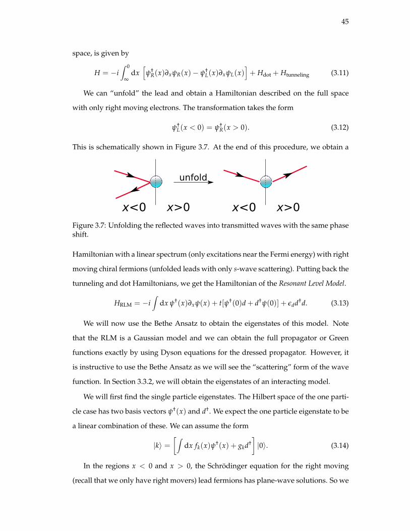
45
space, is given by
H = −i∫ 0
∞dx[
ψ†R(x)∂xψR(x)− ψ†
L(x)∂xψL(x)]
+ Hdot + Htunneling (3.11)
We can “unfold” the lead and obtain a Hamiltonian described on the full space
with only right moving electrons. The transformation takes the form
ψ†L(x < 0) = ψ†
R(x > 0). (3.12)
This is schematically shown in Figure 3.7. At the end of this procedure, we obtain a
x<0 x>0 x<0 x>0
unfold
Figure 3.7: Unfolding the reflected waves into transmitted waves with the same phaseshift.
Hamiltonianwith a linear spectrum (only excitations near the Fermi energy) with right
moving chiral fermions (unfolded leads with only s-wave scattering). Putting back the
tunneling and dot Hamiltonians, we get the Hamiltonian of the Resonant Level Model.
HRLM = −i∫
dx ψ†(x)∂xψ(x) + t[ψ†(0)d+ d†ψ(0)] + ǫdd†d. (3.13)
We will now use the Bethe Ansatz to obtain the eigenstates of this model. Note
that the RLM is a Gaussian model and we can obtain the full propagator or Green
functions exactly by using Dyson equations for the dressed propagator. However, it
is instructive to use the Bethe Ansatz as we will see the “scattering” form of the wave
function. In Section 3.3.2, we will obtain the eigenstates of an interacting model.
We will first find the single particle eigenstates. The Hilbert space of the one parti-
cle case has two basis vectors ψ†(x) and d†. We expect the one particle eigenstate to be
a linear combination of these. We can assume the form
|k〉 =[
∫
dx fk(x)ψ†(x) + gkd
†
]
|0〉. (3.14)
In the regions x < 0 and x > 0, the Schrodinger equation for the right moving
(recall that we only have right movers) lead fermions has plane-wave solutions. So we

46
expect fk(x) ∼ eikx. However, we do expect the solutions to differ for the x < 0 and
x > 0 regions since hopping through the dot will potentially modify the wave function
by a phase. So we will assume the following scattering form for the wave function:
fk(x) = eikx[Aθ(−x) + Bθ(x)]. (3.15)
Acting on our guess with the Hamiltonian, we get
H|k〉 = Ek|k〉
=∫
dx
−i∂xeikx[Aθ(−x) + Bθ(x)] + tgkδ(x)
ψ†(x)|0〉+ [t fk(0) + ǫdgk]d†|0〉.
(3.16)
Before we can solve this equation, we need to establish a regularization convention for
the θ-functions. We define
∂xθ(±x) = ±δ(x), θ(x)δ(x) =1
2δ(x). (3.17)
This regularization can be shown to be consistent with other methods of solution of the
problem, and with any continuous approximations to step functions and δ-functions.
With this, the solution of (3.16) is given by
Ek = k,B
A=
k− ǫd + i t2
2
k− ǫd − i t2
2
, gk =t
k− ǫd(3.18)
Given that themodel is non-interacting, we can immediately write down themulti-
particle states as constructed from a product of single particle states.
|~k〉 = ∏j
|k j〉 (3.19)
In Section 4.3, we carry out a quench where we couple the lead electrons to the dot
at t = 0 and calculate the time evolution of the dot occupation and transient current
as an example of the Yudson representation.
3.3.2 Lieb-Liniger model
The previous model was non-interacting and the S-matrix is trivial, i.e., S = 1. It
doesn’t need the Bethe Ansatz and can be treated by any other means, e.g., the full
47
Green’s functions of the model can easily be obtained, therefore giving access to all
correlation functions and observables. We mention it here since it serves as a simple
example of the Bethe Ansatz method, and more importantly, in Chapter 4, as a simple
example of the Yudson technique.
We now move on to a more complicated interacting integrable model of bosons in
a one dimensional continuum. A brief comment is in order here. The reader might
be aware of several integrable models whose solutions come in the form of using
a transformed set of fields (by Jordan-Wigner transformation, Bogoliubov rotations,
etc.), which become the quasi-particles of the model. In the quasi-particle basis, the
model is non-interacting, and therefore trivially solvable. Examples of this include
the Tonks-Girardeau model [53], the transverse field and longitudinal field Ising mod-
els [25], hard-core bosons on a lattice [32, 33], and the Luttinger liquid [50]. This of
course does not mean that the models are not-interesting or trivial. Especially in the
case of quench dynamics, when the initial state is not best represented in the quasi-
particle basis. We will not be discussing such models in this thesis.
The Lieb-Liniger model cannot be written in terms of non-interacting quasi parti-
cles 4. In this section, we will derive the multi-particle eigenstates of this model. We
will not be interested in the ground state and excitation spectrum of the model. For
more on this, please see Refs. [94, 132, 86].
The model describes bosons on a line interacting via a δ-function potential:
HLL =∫
dx ∂b†(x)∂b(x) + c[b†(x)b(x)]2. (3.20)
The mass of the bosons has been set to 12 . For the c > 0, the potential is repulsive, and
for c < 0, it is attractive. The following applies to either case. The Shrodinger equation
that one obtains for the above Hamiltonian is
[−∂2x + 2c b†(x)b(x)]b†(x) = ∂tb†(x). (3.21)
4By non-interacting, we mean that the quasi-particles must have canonical commutation relations. Itis always possible to write the eigenstates in terms of new creation operators (or fields) that have non-standard commutation relations that are pseudo-momentum dependent. This is precisely the role of theS-matrix.

48
This is called theNon-linear Schrodinger equation and has been studied extensively both
classically and quantum mechanically [43, 86].
Let us begin by assuming a form for the single particle wave functions:
|k〉 = N (k)∫
dx eikxb†(x)|0〉 (3.22)
where we have defined |0〉 as the vacuum containing no particles, and N (k) is a nor-
malization factor. Acting on this state with the Hamiltonian (3.20), we get
HLL|k〉 = −∂2xN (k)eikx = E(k)N (k)eikx (3.23)
giving the stationary solution to the Shrodinger equation with energy E(k) = k2. We
now assume a “Bethe form” for the two-particle wave-functions:
|k1, k2〉 = N (k1, k2)∫
dx1dx2 eik1x1+ik2x2 [θ(x1 − x2) + S12θ(x2 − x1)]b
†(x1)b†(x2)|0〉.
(3.24)
Note that as written, the state is not manifestly symmetric in x1, x2, as it should be for
bosonic fields. We will deal with this momentarily. The important point to note is the
form of the wave function. Since the interaction is active only when the two particles
are on top of each other, in each region x1 > x2 and x1 < x2, there is no interaction
and the Shrodinger equation is solved by plane waves. However, the interaction is
active when the two particle cross – this is captured via the S-matrix S12 that we need
to calculate. This equivalently amounts to a boundary condition when x1 = x2, and is
commonly known as the cusp condition. This approach can be found in Ref. [86]. The
Schrodinger equation for the above state yields
∫
dx1dx2
[
(
−∂2x1 − ∂2x2)
eik1x1+ik2x2 [θ(x1 − x2) + S12θ(x2 − x1)]
+
+ c(1− S12)δ(x1 − x2)eik1x1+ik2x2
]
b†(x1)b†(x2)|0〉
= E(k1, k2)∫
dx1dx2 eik1x1+ik2x2 [θ(x1 − x2) + S12θ(x2 − x1)]b
†(x1)b†(x2)|0〉 (3.25)
Simplifying this using the regularization in (3.17) gives
−i(k1 − k2)(1− S12) + c(1+ S12) = 0, (3.26)
49
which gives
S12 =k1 − k2 + ic
k1 − k2 − ic(3.27)
The energy E(k1, k2) = k21 + k22.
The next step in the process is to write down the multiparticle states. These are
written in general as follows
|~k〉 = N (~k)∫
d~x∑Q
θ(xQ)AQ(~λ)∏j
eikjxjb†(xj)|0〉. (3.28)
where AQ is the phase acquired in going from the ordering x1, x2, . . . , xN to the order-
ing xQ1, xQ2
, . . . , xQN. It is essentially a product of several two particle S-matrix factors.
In this model, since the S-matrices are c-numbers, this condition is trivially satisfied.
It is sufficient to satisfy the three particle condition in order for the multi-particle con-
dition to be satisfied. This is due to the factorizability of all interactions into products
of two particle interactions, a requirement for the integrability of this model. In other
words, the number of particles N =∫
x b†(x)b(x), has to be a conserved quantum
number in order to be able to write down eigenstates with fixed particle number. In
Chapter 5 we write this state in a slightly different form, more conducive for applica-
tion to the Yudson formalism.
The above derivation is valid for both the attractive (c < 0) and the repulsive (c >
0) model since at point we assumed a sign for c. The sign is however crucial and
determines both the nature of the ground state and excitations, as well as the quench
dynamics as we will see in Chapter 5. For c > 0, the spectrum consists of real valued
momenta and the ground state is essentially a Fermi sphere, with the particles obeying
an exclusion principle [94]. The attractive case, however is more interesting as the
spectrum permits momenta in complex conjugate pairs. These correspond to bound
state, or McGuire clusters [94, 139, 99], and we will see these emerge naturally in the
time evolution.
3.4 Bethe Ansatz and quenches
To carry out the computation of the quench dynamics we need to know the eigenstates
of the propagating Hamiltonian. The Bethe Ansatz approach is helpful in this respect

50
as it provides us with the eigenstates of a large class of interacting one dimensional
Hamiltonians. Many of the Hamiltonians that can be thus be solved are of fundamen-
tal importance in condensed matter physics and have been proposed to study various
experimental situations. A partial list includes the Heisenberg chain (magnetism), the
Hubbard model (strong-correlations), the Lieb-Liniger model (cold atoms in optical
traps), the Kondo model, and the Anderson model (impurities in metals, quantum
dots) [11, 96, 94, 6, 7, 136]. For a Hamiltonian to possess eigenstates that are given in
the form of a Bethe Ansatz it must have the property that multi-particle interactions
can be consistently factorized into series of two particle interactions, all of them being
equivalent5.
While originally formulated to understand the Heisenberg chain [11], the technol-
ogy has been studied extensively and recast into a more sophisticated algebraic for-
mulation [129, 86]. The usual focus of the Bethe Ansatz approach has been on the
thermodynamic properties of the system: determining the spectrum, the free energy,
and susceptibilities. Also, considerable efforts weremade to compute correlation func-
tions [133, 86]. In particular, the Algebraic Bethe Ansatz has been used in conjunction
with numerical methods to calculate so-called form factors which allows access to the
dynamical structure functions [103, 24, 61].
Using the Bethe Ansatz to extract dynamics one encounters a triply complicated
problem — the first being to obtain the full spectrum of the Hamiltonian, the second
to calculate overlaps, and the third to carry out the sum, which in some cases involves
sums over large sets of different “configurations” of states. The overlaps are partic-
ularly difficult to evaluate due to the complicated nature of the the Bethe eigenstates
and their normalization. The problem is more pronounced in the far from equilib-
rium case of a quench when the state we start with suddenly finds itself far away from
the eigenstates of the new Hamiltonian [see eq. (2.11)], and all the eigenstates have
non-trivial weights in the time-evolution. In all but the simplest cases, the problem
is non-perturbative and the existing analytical techniques are not suited for a direct
5This set of conditions is known as the Yang-Baxter equation.
51
application to such a situation.
Often quench calculations are carried out in finite volume and the infinite volume
limit is taken at the end of the calculation. This may be necessary for thermodynamic
calculations, as noted, but not for quench dynamics (see sec. 2.3). We shall instead
carry out the quench directly in the infinite volume limit in which case the Yudson
representation allows us to carry out the calculations in an efficient way, doing away
with some of the difficulties mentioned above by not requiring any information about
the spectrum, and by using integration as opposed to discrete summation.
More explicitly, the Schrodinger equation for N bosons H|~λ〉 = ǫ(~λ)|~λ〉 is satis-
fied for any value of the momenta λj, j = 1, · · · ,N if no boundary conditions are
imposed. The initial state can then be written as |Ψ0〉 =∫
dNλ C~λ |~λ〉, with the in-
tegration over ~λ replacing the summation. This is equivalent to summing over an
over-complete basis, the relevant elements in the sum being automatically picked up
by the overlap with the physical initial state.
It is important to note, however, that while the spectrum of an infinite system is
continuous, it can still be very complicated. This is indeed the case with several inte-
grable models, including the Lieb-Liniger model, where the analytic structure of the
S-matrix (the momentum dependent phase picked up when two particles cross) may
permit momenta in the form of complex-conjugate pairs signifying bound states. In
the formalism we employ, such states are taken into account by appropriately choos-
ing the contours of integration in the complex plane. We have now developed the base
to go on and understand this formalism.

52
Chapter 4
The Yudson representation
4.1 A complete basis in infinite volume
As seen in Section 3.4, time evolving arbitrary initial states is complicated even in the
case of an integrable model where we know the eigenstates. Our goal is to try and
circumvent some of the issues that make this process complicated. In view of the
discussion in Section 2.3, it is meaningful to talk about quenches directly in the infinite
volume limit. This leads to one simplification that there are no boundary conditions,
and consequently, no Bethe Ansatz Equations to solve. In other words, the spectrum
is not quantized, and it makes sense to talk about eigenstates of the Hamiltonian for
any values of the momentum1.
Our goal is to find a representation for arbitrary states in terms of a complete basis
directly in the infinite volume limit. For a generic state |Ψ0〉, we expect to write down
something like
|Ψ0〉 =∫
Dλ |λ〉 〈λ|Ψ0〉 , (4.1)
where Dλ denotes both the integration measure and the domain. We have replaced
the sum over eigenstates by an integral since the eigenvalues are no longer constrained
by boundary conditions or finite size2.
As an example, let’s see how this works in a model of free fermions on an infinite
line. The Hamiltonian is
HFF =∫
kǫkc
†kck (4.2)
1More correctly, the rapidity, which coincides with the physical momentum for some models.
2In the thermodynamic limit of an infinite number of particles, even with periodic boundary condi-tions, the discrete sum becomes an integral over an appropriately definedweighting function [140]. Here,we are referring to a finite number of particles and infinite volume, and so this is a different situation. Wecan write an integral since the momenta are not quantized by boundary conditions.
53
and the eigenstates are
|k〉 = ∏j
c†kj |0〉 =∫
∏j
dyj eikjyjc†(yj)|0〉. (4.3)
If we write a generic initial state as |Ψ0〉 = ∏j c†(xj)|0〉, we see that
1
N!
∫
[
∏j
dk j
2π
]
|k〉 〈k|Ψ0〉
=1
N! ∑P
(−1)P∫
yj
∫ ∞
−∞
[
∏j
dk j
2π
]
∏j
eikj(yj−xPj )c†(yj)|0〉
=1
N! ∑P
(−1)P∫
yj∏j
δ(yj − xPj)c†(yj)|0〉
=1
N! ∑P
(−1)P ∏j
c†(xPj)|0〉
= |Ψ0〉
(4.4)
On the lattice, the integral over k will be restricted to the first Brillouin Zone,
k ∈ [−π,π], and the Dirac delta function above gets replaced by a Kronecker delta
function. While the free fermion case might seem rather trivial, we will see that more
complicated models can also be dealt with in this fashion.
The central aspect of the above formula is determining the measure of integration
and the domain, or integration paths. While it might seem that since the momenta are
not quantized, we can integrate over the entire allowed range of momenta, a compli-
cation arises for integrable models. Recall that for many integrable models, when we
solve for the spectrum (or momentum eigenvalues) of a finite sized model, we end up
with solutions in the form of complex conjugate pairs. These are the so-called string
solutions, and in the Lieb-Liniger model, e.g., correspond to bound states (more on this
in Chapter 5). In order for (4.1) to be a valid representation, these complex values must
be taken into account. The integration paths must therefore be allowed to explore the
complex plane, in a controlled fashion. The key, as we will see, is to exploit the poles of
the S-matrix and choose contours such that they give zero residues when integrated.
54
4.2 The Yudson integral representation
The integral representation described here was originally developed by Yudson [142,
143] to understand superradiance in the Dicke model [40], when he noticed that the
sum over the eigenstates fell into a certain pattern that could be obtained by calculating
residues at appropriate poles [141]. These poles are dictated by the two-particle S-
matrix (see Section 3.2) of the Dicke model, which is integrable.
Depending on the particular model, certain changes have to be made to the rep-
resentation, in particular, the integration measure, and the paths or “contours” of in-
tegration. Here, I describe some generalities of the representation, and then we’ll see
some examples.
First, in order to simplify the overlap of a Bethe eigenstate and the initial state, we
write the initial state in an ordered way as
|Ψ0〉 = θ(x1 > x2 > · · · > xN)∏j
c†(xj)|0〉. (4.5)
This can be done in general:
∏j
c†(xj) = ∑P
θ(xP1 > xP2 > · · · > xPN ∏j
c†(xj)
= ∑P
θ(x1 > x2 > · · · > xN)∏j
c†(xPj)
= ∑P
ζPθ(x1 > x2 > · · · > xN)∏j
c†(xj)
(4.6)
with ζ = ± depending of whether the particles are bosons or fermions.
Further, we modify (4.1) to
|Ψ0〉 =∫
Dλ |λ〉(λ|Ψ0〉 (4.7)
where (λ| corresponds to a modified eigenstate, where again, we order the particles.
That is, if the eigenstate of the model were given by
|λ〉 =∫
yφ(y,λ)∏
j
c†(yj)|0〉, (4.8)
then,
|λ) =∫
yθ(y1 > y2 > · · · > yN)φ(y,λ)∏
j
c†(yj)|0〉. (4.9)

55
In the above case of free fermions, the main simplification this achieves is to remove
the sum over permutations in (4.4). However, in more complex interacting models,
this step achieves a greater simplification, by eliminating the S-matrix in |λ〉.
The next important step is determining the integration measure, and a set of con-
tours of integration. Not explicitly visible in the representation is the fact that one has
to write the Bethe Ansatz eigenstates in an appropriate parametrization. The reason
for this is that the choice of contours depends on the analytic structure of the S-matrix.
As mentioned in Chapter 3, the analytic structure of the S-matrix determines whether
a particular model admits complex valued momenta, or bound states. We will see that
the Yudson representation will automatically tell us this. However, in order to write
down a useful Yudson representation, the choice of contours has to be reasonable and
that puts some constraints on the pole-structure of the S-matrix. Parametrizing for a
simple pole structure typically complicates the single particle states, however3. Each
model will therefore require a separate proof of the validity of (4.7), but below I will
outline the general idea.
As discussed in Section 3.2, Bethe Ansatz eigenstates have a typical form, where the
wave-functions are separated into different configuration sectors, and the sectors are
related to each other via phases. These phases are products of two particle S-matrices
that correspond to the phase acquired when two particles cross each other. The fact
that any two sectors are related via such a product is due to the factorizability of the
interactions and is a hallmark of Bethe Ansatz integrable models.
Writing a generic eigenstate as
|λ〉 =∫
y∑Q
θ(yQ)AQ(λj)∏j
φ(yj,λj)c†(yj)|0〉 (4.10)
where c†(yj) are either bosonic or fermionic4. We set AI = 1, so that
|λ) =∫
yθ(yI)∏
j
φ(yj,λj)c†(yj)|0〉 (4.11)
3See p.523-527 of Ref. [136] for the parametrizations that provide a simple S-matrix pole structure forvarious models.
4For impurity models, or models with multiple species, the single particle creation operators are morecomplicated, but the method is straightforward to generalize. We study an impurity model in detail inthe next section.
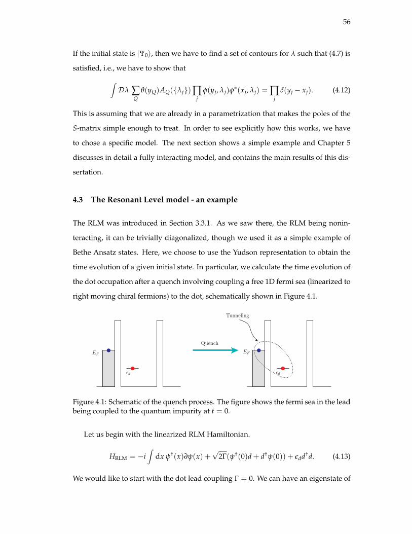
56
If the initial state is |Ψ0〉, then we have to find a set of contours for λ such that (4.7) is
satisfied, i.e., we have to show that
∫
Dλ ∑Q
θ(yQ)AQ(λj)∏j
φ(yj,λj)φ∗(xj,λj) = ∏
j
δ(yj − xj). (4.12)
This is assuming that we are already in a parametrization that makes the poles of the
S-matrix simple enough to treat. In order to see explicitly how this works, we have
to chose a specific model. The next section shows a simple example and Chapter 5
discusses in detail a fully interacting model, and contains the main results of this dis-
sertation.
4.3 The Resonant Level model - an example
The RLM was introduced in Section 3.3.1. As we saw there, the RLM being nonin-
teracting, it can be trivially diagonalized, though we used it as a simple example of
Bethe Ansatz states. Here, we choose to use the Yudson representation to obtain the
time evolution of a given initial state. In particular, we calculate the time evolution of
the dot occupation after a quench involving coupling a free 1D fermi sea (linearized to
right moving chiral fermions) to the dot, schematically shown in Figure 4.1.
Quench
EF
ǫd
EF
ǫd
Tunneling
Figure 4.1: Schematic of the quench process. The figure shows the fermi sea in the leadbeing coupled to the quantum impurity at t = 0.
Let us begin with the linearized RLM Hamiltonian.
HRLM = −i∫
dx ψ†(x)∂ψ(x) +√2Γ(ψ†(0)d+ d†ψ(0)) + ǫdd
†d. (4.13)
We would like to start with the dot lead coupling Γ = 0. We can have an eigenstate of

57
N right moving electrons in the lead:
|k〉 =∫
dNx ∏j
eikjxjψ†(xj)|0〉 (4.14)
One can check that the above is indeed an eigenstate of the uncoupled lead for any set
k j with E = ∑j k j.
At t = 0, we couple the lead to the dot. The above state then becomes the initial
state that we want to evolve in time. Before we move on to time-evolve, let’s rewrite
the initial state in a way that’s in line with the form of the Yudson representation.
Inserting unity as a sum over different orderings of the xj, and some manipulation, we
obtain
|k〉 =∫
dNx ∑P
sgn(P)∏j
eikPj xj |~x〉, (4.15)
where
|x〉 = θ(x1 > x2 > · · · > xN)∏j
ψ†(xj)|0〉. (4.16)
The state |x〉 is now in a form that can be plugged into the Yudson representation,
which we will now proceed to obtain.
4.3.1 Yudson representation for the RLM
The RLM being a noninteracting model, the Yudson representation is in some sense
trivial. However, the approach of directly evolving an initial state gives us complete
control over the process, rather than having to start with a ground state. In particular,
it gives us the ability to start with states with different symmetries, entanglement, and
so on. Since we are using the RLM as an example of time evolution using the Yudson
representation, we will study the simple case described above.
Consider the initial state |x〉 described above. It is straightforward to check that
|x〉 = 1
(2π)N
∫
dNy∫
dNk ∏j
eikj(yj−xj)k j − ǫd − iΓ sgn(yj)
k j − ǫd + iΓ
k j − ǫd + iΓ sgn(xj)
k j − ǫd − iΓψ†(yj)|0〉. (4.17)
For any xj < 0 there is a pole at k∗j = ǫd − iΓ for yj > 0. Since yj − xj > 0, we can carry
out the integration by closing the contour in the upper half plane giving us a residue
58
of zero, since there is no pole in this region. For yj < 0 all the poles are canceled,
and we can carry out the integration to obtain 2πδ(yj − xj). For xj > 0, the pole is at
k∗j = ǫd + iΓ for yj < 0. Again these two constraints imply that yj < xj, and closing the
contour in the lower half plane give a zero residue. For yj > 0, there are no poles, and
we can carry out the integral to obtain 2πδ(yj − xj). We have therefore shown that the
above identity is indeed true. We have ignored the “dot” part of the eigenstate, but it
is easy to show that it produces no contribution.
The lead part of state at time t is therefore given by
|x, t〉l = e−iHRLMt|x〉
=1
(2π)N
∫
dNy∫
dNk ∏j
eikj(yj−xj−t) k j − ǫd − iΓ sgn(yj)
k j − ǫd + iΓ
× k j − ǫd + iΓ sgn(xj)
k j − ǫd − iΓψ†(yj)|0〉.
(4.18)
Using arguments above, we can show that the above integral is nonzero for yj < xj + t,
which we interpret as a causality constraint. In this region, the integration can easily
be carried out via the residue theorem, and is provided below.
4.3.2 Time evolution of the dot occupation
The state at arbitrary time t is given by
|x, t〉 = θ(x1 > · · · > xN)∫
dNyN
∏j=1
(
F(yj, xj, t)ψ†(yj) + G(xj, t)δ(yj)d
†)
|0〉, (4.19)
where
F(y, x, t) = δ(y− x− t)− 2Γθ(x < 0 < y < x+ t)e(Γ+iǫd)(y−x−t), (4.20)
G(x, t) = −i√2Γθ(x < 0 ≤ x+ t)e−(Γ+iǫd)(x+t). (4.21)
Now we can go back to our initial state and find the out state corresponding to it as
|k, t〉 =∫
dNx ∑P
sgn(P)∏j
eikPj xj |x, t〉. (4.22)
There are two things to note here. One is that the state |x, t〉 can be simplified, since
terms in the product with multiple d†s are identically zero (Pauli exclusion). We can

59
thus expand the product and write down
|x, t〉 = θ(x1 > · · · > xN)∫
dNy
( N
∏j=1
F(yj, xj, t)ψ†(x1) . . . ψ†(yN)+
+N
∑k=1
∏j 6=k
F(yj, xj, t)G(xk, t)δ(yk)ψ†(y1) . . . d
†(k) . . . ψ†(yN)
)
|0〉.(4.23)
The subscript k on d† indicates that it occurs in the k-th position. This can be fur-
ther simplified by rearranging the terms in the sum so d† always appears in the end.
One can then swap yk and yN in each term (since the y are dummy variables that we
integrate over, this is just a change of variables). For all k 6= N this swapping of the
positions k and N gives us a minus sign due to the complete antisymmetry of the state.
We get,
|x, t〉 = θ(x1 > · · · > xN)∫
dNy(
F(y, x, t)ψ†(y1) . . . ψ†(yN)+
+G(y, x, t)δ(yN)ψ†(y1) . . . ψ†(yN−1)d
†)
|0〉,(4.24)
where
F(y, x, t) =N
∏j=1
F(yj, xj, t), (4.25)
G(y, x, t) =N−1
∏j=1
F(yj, xj, t)G(xN , t)− (4.26)
−N−1
∑k=1
F(y1, x1, t) . . . F(yk, xN , t) . . . F(yN−1, xN−1, t)G(xk). (4.27)
Recall that we eventually Fourier transform the xj, so they are also dummy variables
and we can do a change of variables. To be more precise we can reverse the steps used
to write the initial state in a particular sector. We end up anti-symmetrizing the F and
G in x.
The second point to note is that after the Fourier transform, we get a multiparticle
state, where the momenta of each particle are localized by a delta function. In other
words,
〈k|k〉 = ∑P
sgn(P)∏j
δ(kPj − k j). (4.28)
These are bad states to work with when we take expectation values since we get δ(0)
type of infinities. Further, the integrals that appear in the Yudson representationwould

60
diverge in a norm without suitable regularization. We would therefore, instead, like
to work with Gaussian wave packets localized in position space, so we have normal-
izable wave functions, and then take the limit of the width of the Gaussian going to
infinity. Consider the following as an incoming state:
|k〉 =N
∏j=1
1
(2π)1/2
∫
dxj eikjxj−
x2j
4σ2 ψ†(xj)|0〉 (4.29)
The norm of the state is
〈k|k〉 = ∑P
sgn(P)∏j
σ√2π
e−(kPj−kj)
2σ2/2. (4.30)
In the limit of σ → ∞, we get back the above result for plane waves.
We are interested in the specific case of the initial momenta being chosen from a
filled Fermi sea (think about periodic boundary conditions on a circle of length L).
The momenta, therefore are,
k j = −2π j
L(4.31)
In the σ → ∞ limit, the above norm reduces to δ(k j − kPj) =L2π δjPj .
We will work with finite σ, and make series expansion in 1/σ where applicable
and retain only first order terms. We will then choose the momenta from a Fermi sea
and take the limit of σ → ∞. Now that we have well defined states, we can go ahead
and ask questions about expectation values. In particular, we will be interested in
computing the expectation value for the dot occupation,
〈nd〉 = 〈k, t|d†d|k, t〉. (4.32)
What we’re therefore interested in computing is the quantity 〈x′, t|d†d|x, t〉. We can
then carry out the Fourier transform w.r.t xi and x′i with momenta ki. We will take the
spread of the Gaussian weight, σ to be very large wherever necessary. From eq. (4.24),
we get,
〈x′, t|d†d|x, t〉 = θ(x1 > · · · > xn)θ(x′1 > · · · > x′N)
∫
dN−1y ∑P
sgn(P)G∗(Py, x′, t)G(y, x, t), (4.33)

61
where P in the above equation denotes permutation on 1, . . . ,N − 1.
One could alternatively first Fourier transform the state at time t. This is a better
approach if we can carry out the x integrals analytically. There is one glitch due to the
ordering θ(x1 > x2 > · · · > xN). We’ll sort this out below. Consider just the lead part
of the state at time t:
|k, t〉l =1
(2π)N/2
∫
dNy dNx θ(x1 > · · · > xN)
∑P
sgn(P)∏j
eikjxPj−x2j /4σ2
F(x, y, t)∏j
ψ†(yj)|0〉. (4.34)
The F(x, y, t) can be anti-symmetrized in y. Let us call
FA(x, y, t) =1
N! ∑P
sgn(P)F(x, Py, t). (4.35)
The structure of F in the case of free particles (and we believe in general) is such that
anti-symmetrizing in y automatically makes it antisymmetric in x also. For the non-
interacting case, this is obvious as F is just a product of 1 particle wave functions. Thus
in eq (4.34) above, the whole integrand (without the θ function) is now symmetric in
x. It therefore simplifies to
|k, t〉l =1
(2π)N/2N!
∫
dNy dNx ∑P
sgn(P)∏j
eikjxPj−x2j /4σ2
FA(x, y, t)∏j
ψ†(yj)|0〉. (4.36)
For the free particle case, the integrals over x now factorize and can be carried out ex-
actly. Once this is done, the overlaps will be easier to evaluate (ywill be the remaining
integration variable, and t is the parameter. k j will have to be specified.)
So, we will now try to carry out the above Gaussian integration explicitly. Writing
out eq. (4.36) more explicitly, we have,
|k, t〉l =1
(2π)N/2(N!)2 ∑P,Q
sgn(P) sgn(Q)
∫
dNy I(kP, yQ, t)∏j
ψ†(yj)|0〉, (4.37)

62
where
I(kP, yQ, t) = ∏j
∫
dxj eikPj xj−x2j /4σ2
F(xj, yQj, t). (4.38)
The integral over xj above is trivial to carry out. The result is
I(kP, yQ, t) = ∏j
(
eikPj (yQj
−t)−(yQj−t)2/4σ2
− 2Γ√
πσ2θ(0 < yQj< t)
e−(Γ+iǫd)(t−yQj
)−(kPj−ǫd+iΓ)2σ2
(
erf((t− yQj)/2σ + i(kPj − ǫd + iΓ)σ)− erf(i(kPj − ǫd + iΓ)σ)
)
)
(4.39)
We also have
〈k, t|d†d|k, t〉 = 〈k, 0|k, 0〉 − l〈k, t|k, t〉l. (4.40)
We have one last formula to obtain, i.e., l〈k, t|k, t〉l . The overlap introduces some re-
dundancy in the permutations, and we can easily get rid of it with a factor of N!. We
get,
l〈k, t|k, t〉l =1
(2π)N(N!)2 ∑P,P′,Q
sgn(P) sgn(P′) sgn(Q)
∫
dNy I∗(kP′ , yQ, t)I(kP, y, t). (4.41)
For the above form of I, antisymmetrizing in k automatically antisymmetrizes in y. We
thus end up with,
l〈k, t|k, t〉l =1
(2π)NN! ∑P,P′
sgn(P) sgn(P′)
∫
dNy I∗(kP′ , y, t)I(kP, y, t). (4.42)
However, we can now move the anti-symmetrization to the y, and get
l〈k, t|k, t〉l =1
(2π)NN! ∑P,P′
sgn(P) sgn(P′)∫
dNy I∗(k, yP′ , t)I(k, yP, t). (4.43)
But now we’re back to having redundancy since y is just an integration variable. We
finally get
l〈k, t|k, t〉l =1
(2π)N ∑P
sgn(P)∫
dNy I∗(kP, y, t)I(k, y, t). (4.44)

63
Going back to our initial state at finite σ, we can write
〈k, 0|k, 0〉 = det A, (4.45)
where Apk = σ√2π
e−(k−p)2σ2/2. In the limit σ → ∞, Apk → δ(p − k). For the time
evolved state we have,
|k, t〉l =N
∏j=1
∫
dyj f (k j, yj, t)ψ†(yj)|0〉. (4.46)
where f is just shorthand for the wave function above.
As noted above, we’re interested in computing the norm of the above wave func-
tion. We have,
〈nl(t)〉 = det(A+ ΓDD†) (4.47)
where D is a column vector where the index is the momentum 5. After some simplifi-
cation (involving taking leading order in 1/σ and some algebraic manipulation), it is
given by
Dk = 2ei(k+iΓ)t/2t sinc((k− ǫd + iΓ)t/2) (4.48)
It is also important that the entries inDD† (a squarematrix) have awell defined σ → ∞
limit - in fact they are independent of σ. The matrix determinant lemma [22] allows us
to write
〈nl(t)〉 = det(A)(1+ D†A−1D). (4.49)
In the large σ limit, A becomes the identity matrix (times L/2π), and we have a very
simple expression for nl . We now assign k j = −2π j/L, where L is the length of system
where we choose the initial state from. After some manipulation we get the evolution
of the dot occupation after a quench:
〈nd(t)〉 =2Γ
L ∑j
(
1− 2e−tΓ cos(t(k j − ǫd)) + e−2tΓ
Γ2 + (k j − ǫd)2
)
. (4.50)
5Note that since the k are going to be chosen from a Fermi sea with a finite number of electrons, N, wecan always think in terms of finite matrices. The thermodynamic limit will be taken in the end. When wesay index, we mean the j in k = −2π j/L.

64
This can be converted to an integral in the thermodynamic limit, and we can also take
the cut-off D ∼ N/L to infinity. This gives us
〈nd(t)〉 =e−tΓ
2π
(
cosh(tΓ)(
π − 2 arctan(ǫd/Γ)−
iCi(t(ǫd − iΓ)) + iCi(t(ǫd + iΓ)))
+ sinh(tΓ)(
π−
Si(t(ǫd + iΓ)) + iSi(t(−ǫd + iΓ)))
)
(4.51)
Figure 4.2 shows the dot occupation as a function of time, and Figure 4.3 shows the
dot occupation starting with two different initial states, one having the dot occupied.
We see that starting with the dot occupied has no effect on the final state, due to the
infinite lead acting as a thermal reservoir for the dot.
2 4 6 8 10 12 14t
0.2
0.4
0.6
0.8
X n d \
G = 0.6 , Εd =- 1.2
G = 0.6 , Εd = 1.2
G = 0.2 , Εd =- 1.2
G = 0.2 , Εd = 1.2
Figure 4.2: Time evolution of dot occupation. The different curves correspond to dif-ferent values of Γ and ǫd. The dot is easier to occupy when the energy level is belowthe fermi level of the leads. The time scale to reach the asymptotic value is τ ∼ 1/Γ.
4.3.3 Note on finite systems
In the discussion in Section 4.3.2, we implicitly managed to get results for finite vol-
ume, and then take a thermodynamic limit. This is interesting, given that the Yudson
representation is valid only in the infinite volume limit. Of course, we can perfectly
well take the initial condition to have some finite extent. We started out with an initial

65
5 10 15 20 25t
0.2
0.4
0.6
0.8
1.0
X n d \
G = 0.1 , Εd =- 1.5 , dot occ . at t = 0
G = 0.1 , Εd =- 1.5 , dot empty at t = 0
G = 0.1 , Εd = 1.5 , dot occ . at t = 0
G = 0.1 , Εd = 1.5 , dot empty at t = 0
Figure 4.3: Time evolution of dot occupation for different initial states. Note that theinitial state does not affect the asymptotic dot occupation. This is because the leadessentially acts as an infinite thermal reservoir and the system loses memory of theinitial state.
state that was a free Fermi sea
|Ψ0〉 = ∏k
c†k |0〉. (4.52)
If we start with the initial state defined on a ring of length L with N particles, then
k j = −2π j
L, j = 1, · · · ,N. (4.53)
What is interesting, however, is that inspite of the eigenstates used for time evolution
being from the infinite volume basis, the observable calculated, 〈nd〉, picks out the
eigenvalues corresponding to a finite length L system. We suspect that this might
be a feature specific to this model because of the noninteracting nature, i.e., different
momentummodes do not mix, and the quantum impurity has anO(1/L) effect on the
physics of the leads. Further, since we can carry out the calculation for finite time, it is
meaningful to first take the large N limit, giving us a true thermodynamic limit of the
problem.
4.4 Application to other integrable models
The previous section showed the Yudson method applied to a noninteracting model.
Everything could have been achieved without recourse to it. In the next two Chapters,
we’ll see the Yudson representation applied to interacting integrable models which
66
cannot be mapped to a noninteracting model. Here I would like to outline the Yudson
representation for some other models that are of interest.
The key to the Yudson representation is finding an appropriate set of integration
contours. In principle the representation should be possible for any integrable model.
It would therefore be very interesting to generalize the approach to the Sine-Gordon
model (bosons with a periodic potential), Anderson impurity model (interacting im-
purity model that displays the Kondo effect), the Kondo model, the fermionic Hub-
bard model, etc. Work is currently underway on a few of these. I will briefly outline
the specific issues that emerge in using the approach for the Anderson model.
4.4.1 Anderson impurity model
The Anderson impurity model is a simple model of Kondo physics in one dimension.
A noninteracting lead of spinful electrons is coupled to a two level impurity that has
an onsite Coulomb interaction. The linearized and unfolded (see Section 3.3.1) Hamil-
tonian is given by
HAIM = −i∫
dx ψ†al∂xψal + tl [ψ
†alda + d†aψal ] + ǫdd
†ad+Ud†↑d↑d
†↓d↓. (4.54)
a is a spin index and l is a lead or flavor index. The interaction only couples up
and down spins due to Pauli exclusion. The model is exactly solvable via the Bethe
Ansatz [138]. In the limit of infinite Coulomb repulsion, or the strongly interacting
limit, the dot occupation is restricted to 0 or 1, and the S-matrix simplifies to
Sij =ki − k j + iPij
ki − k j + i. (4.55)
It is trivial for two particles in a triplet (or spin symmetric) state. As such, it is straight-
forward to come up with a set of Yudson contours for this problem, and they are
similar to the case of the Dicke model [142] or the attractive Lieb-Liniger model that
we study in the next chapter. The complication arises from the fact that the S-matrices
are not c-numbers and a multiparticle S-matrix cannot be written as a generic prod-
uct of two particle S-matrices, since the ordering is important. A further complication
is produced by the fact that for generic initial states, the spin permutation operators
67
generate new states with permuted spin indices, and the book keeping is highly com-
plicated. We are currently trying to study alternative formulations in order to deal
with this issue.
It must however be mentioned that in principle the problem is solvable. If an ef-
ficient numerical algorithm is developed to keep track of the matrices and carry out
the contour integrations, then we can indeed calculate relevant physical quantities. In
that sense, it is an improvement over other analytical techniques where the difficulties
are in the formulation stage.
68
Chapter 5
Quench dynamics of the Lieb-Liniger model
This Chapter studies the time-evolution of interacting bosons following a quench from
a few different initial states. Most of the material here appears in Refs. [71] and [72].
5.1 The Lieb-Liniger model
Bosons in one dimensional traps interact via short range potentials, which can be
well approximated by a δ-function interaction. This model was solved in 1963 by
Lieb and Liniger [94] who originally introduced it to overcome shortcomings of other
models and approaches for understanding quantum gases and liquids, and to pro-
vide a rigorous result to test perturbation theory against. In particular, they sought to
improve upon Girardeau’s hard-core boson model [53] by providing a tunable para-
meter and better model a low density gas, perhaps extensible to higher dimensions.
The Schrodinger equation for the model is also commonly known as the Non-linear
Schrodinger equation and has been extensively studied both classically and quantum
mechanically.
The Hamiltonian is given by
H =∫
x[∂b†(x)∂b(x) + c b†(x)b(x)b†(x)b(x)], (5.1)
where b is a bosonic field and c is the interaction strength. The mass has been set to
1/2. The action for the model ∼∫
x,t[∂t − ∂2x]. Time therefore has the dimension of
(length)2. The coupling constant c has the dimensions of length.
The model is integrable and the eigenstates take the Bethe Ansatz form,
|~λ〉 = N(~λ)∫
x∏i<j
Zxij(λi − λj)∏
j
eiλjxjb†(xj)|0〉, (5.2)

69
where N(λ) is a normalization factor determined by a particular solution, and
Zxij(z) =
z− ic sgn(xi − xj)
z− ic(5.3)
incorporates the two particle S-matrix, Sij =λi−λj+ic
λi−λj−ic occurringwhen two bosons cross.
The above state satisfies
H|~λ〉 = ∑j
λ2j |~λ〉 (5.4)
for any value of the momenta~λ, which, depending on the sign of c, may be pure real
or form complex pairs. In our work, we study the evolution dynamics of the model on
the infinite line and need not solve for explicit distributions of the~λ that characterize
the low lying energy eigenstates, as discussed in section 2.3.
5.2 Yudson representation
In 1985, V. I. Yudson presented a new approach to time evolve the Dicke model (a
model for superradiance in quantum optics [40]) considered on an infinite line [142].
The dynamics in certain cases was extracted in closed form with much less work than
previously required, and in some cases where it was even impossible with earlier
methods. The core of the method is to bypass the laborious sum over momenta us-
ing an appropriately chosen set of contours and integrating over momentum variables
in the complex plane. It is applicable in its original form to models with a particular
pole structure in the two particle S-matrix, and a linear spectrum. We generalize the
approach to the case of the quadratic spectrum and apply it to the study of quantum
quenches.
As discussed earlier, in order to carry out the quench of a system given at t = 0 in
a state |Ψ0〉 one naturally proceeds by introducing a “unity” in terms of a complete set
of eigenstates and then apply the evolution operator,
|Ψ0, t〉 = e−iHt ∑λ
|~λ〉〈~λ|Ψ0〉 = ∑λ
e−iǫ(~λ)t|~λ〉〈~λ|Ψ0〉 (5.5)
The Yudson representation overcomes the difficulties in carrying out this sum by using
an integral representation for the complete basis directly in the infinite volume limit.

70
In the following two sections, we will discuss the representation for the repulsive
and attractive models. Each will require a separate set of contours of integrations in
order for the representation to be valid. We will notice that in the repulsive case, it
is sufficient to integrate over the real line. The attractive case will require the use of
contours separated out in the imaginary direction (to be qualified below) consistent
with the fact that the spectrum consists of “strings” with momenta taking values as
complex conjugate pairs [94].
5.2.1 Repulsive case
We begin by discussing the repulsive case, c > 0. For this case, a similar approach has
been independently developed in Ref. [134] and has been used by Lamacraft [90] to
calculate noise correlations in the repulsive model. We will start with a generic initial
state given by
|Ψ0〉 =∫
~xΦs(~x)∏
j
b†(xj)|0〉. (5.6)
with Φs symmetrized. Using the symmetry of the bosonic operators, we can rewrite
this state in terms of N-boson coordinate basis states,
|Ψ0〉 = N!∫
~xΦs(~x)|~x〉 (5.7)
where,
|~x〉 = θ(~x)∏j
b†(xj)|0〉. (5.8)
with θ(~x) = θ(x1 > x2 > · · · > xN). It suffices therefore to show that we can express
any coordinate basis state as an integral over the Bethe Ansatz eigenstates
|~x〉 = θ(~x)∫
γ∏j
dλj
2πA(~λ,~x)|~λ〉 (5.9)
with appropriately chosen contours of integration γj and A(λ,~x), which plays a role
similar to the overlap of the eigenstates and the initial state.
We claim that in the repulsive case equation (5.9) is realized with
A(~λ,~x) = ∏j
e−iλjxj . (5.10)

71
and the contours γj running along the real axis from minus to plus infinity. In other
words eqn. (5.9) takes the form,
|~x〉 = θ(~x)∫
~y
∫
∏j
dλj
2π ∏i<j
Zyij(λi − λj)∏
j
eiλj(yj−xj)b†(yj)|0〉. (5.11)
Equivalently, we claim that the λ integration above produces ∏j δ(yj − xj).
We shall prove this in two stages. Consider first yN > xN . To carry out the integral
using the residue theorem, we have to close the integration contour in λN in the upper
half plane. The poles in λN are at λj − ic, j < N. These are all below γN and so the
result is zero. This implies that any non-zero contribution comes from yN ≤ xN . Let
us now consider yN−1 > xN−1. The only pole above the contour is λ∗N−1 = λN + ic.
However, we also have, yN−1 > xN−1 > xN ≥ yN =⇒ yN−1 > yN . This causes
the only contributing pole to get canceled. The integral is again zero unless yN−1 ≤xN−1. We can proceed is this fashion for the remaining variables thus showing that the
integral is non-zero only for yj ≤ xj.
Now consider y1 < x1. We have to close the contour for λ1 below. There are no
poles in that region, and the residue is zero. Thus the integral is non-zero for only
y1 = x1. Consider y2 < x2. The only pole below, at λ∗2 = λ1 − ic is canceled as before
since we have y2 < x2 < x1 = y1. Again we get that the integral is only non-zero for
y2 = x2. Carrying this on, we end up with
θ(~x)∫
~y∏j
δ(yj − xj)b†(yj)|0〉 = |~x〉. (5.12)
In order to time evolve this state, we can act on it with the unitary time evolution
operator. Since the integrals are well-defined we can move the operator inside the
integral signs to obtain,
|~x, t〉 = θ(~x)∫
∏j
dλj
2πe−iǫ(~λ)tA(~λ,~x)|~λ〉. (5.13)
5.2.2 Attractive case
We now consider an attractive interaction, c < 0. As mentioned earlier, this changes
the spectrum of the Hamiltonian, allowing complex, so-called string solutions, which in

72
Im(λ)
Re(λ)
λ1
λ2
λ3
∞
∞
Figure 5.1: Contours for the λ integration. Shown here are three contours, and theclosing of the Nth (here, third) contour as discussed in the proof.
this model, correspond to many-body bound states. In fact, the ground state at T = 0
consists of one N-particle bound state. We will see how the Yudson integral represen-
tation takes this into account. Similar properties are seen to emerge in [114], where
the authors obtain a propagator for the attractive Lieb-Liniger model by analytically
continuing the results obtained by Tracy and Widom [134] for the repulsive model.
One will immediately notice from the eigenstates that the pole structure of the S-
matrix is altered. This change prevents the proof of the previous section fromworking.
In particular, the poles in the variable λN are at λj + i|c| for j < N, and the residue of
the contour closed in the upper half plane is not zero any more. We need choose a
contour to avoid this pole. This can be achieved by separating the contours in the
imaginary direction such that adjacent Im[λj − λj−1] > |c|. At first sight, this seems
to pose a problem as the quadratic term in exponent diverges at large positive λ and
positive imaginary part. There are two ways around this. We can tilt the contours as
shown in Fig. 5.1 so that they lie in the convergent region of the Gaussian integral. The
pieces towards the end, that join the real axes though essential for the proof to work
at t = 0, where we evaluate the integrals using the residue theorem, do not contribute
at finite time as the integrand vanishes on them as they are taken to infinity. Another
more natural means of doing this is to use the finite spatial support of the initial state.
The overlaps of the eigenstates with the initial state effectively restricts the support for

73
the λ integrals, making them convergent.
The proof of equation (5.9) now proceeds as in the repulsive case. We start by
assuming that yN > xN requiring us to close the contour in λN in the upper half plane.
This encloses no poles due to the choice of contours and the integral is zero unless
yN ≤ xN . Now assume yN−1 > xN−1. Closing the contour above encloses one pole at
λ∗N−1 = λN − i|c|, however since yN−1 > xn−1 > xN ≥ yN , this pole is canceled by
the numerator and again we have yN−1 ≤ xN−1. We proceed in this fashion and then
backwards to show that the integral is non-zero only when all the poles cancel, giving
us ∏j δ(yj − xj), as required.
5.3 Two particle dynamics
We begin with a detailed discussion of the quench dynamics of two bosons. As we
saw, it is convenient to express any initial state in terms of an ordered coordinate basis,
|~x〉 = θ(x1 > x2 > · · · > xN)∏j b†(xj)|0〉. At finite time, the wave function of bosons
initially localized at x1 and x2 and subsequently evolved by a repulsive Lieb-Liniger
Hamiltonian is given by,
|~x, t〉2 = e−iHtθ(x1 − x2)b†(x1)b
†(x2)|0〉
=∫
y,λZy12(λ1 − λ2)e
−iλ21t−iλ2
2t+iλ1(y1−x1)+iλ2(y2−x2)
× b†(y1)b†(y2)|0〉
=∫
y
ei(y1−x1)
2
4t +i(y2−x2)
2
4t
4πit
×[
1− c√
πitθ(y2 − y1)ei8t α2
erfc
(
i− 1
4
iα√t
)
]
× b†(y1)b†(y2)|0〉.
(5.14)
where α = 2ct− i(y1 − x1)− i(y2 − x2). The above expression retains the Bethe form
of wave functions defined in different configuration sectors. The only scales in the
problem are the interaction strength c and the scale from the initial condition, the sep-
aration between the particles at t = 0.
In order to get physically meaningful results we need to start from a physical initial

74
state. We choose first the state |Ψ(0)latt〉 where bosons are trapped in a periodic trap
forming initially a lattice-like state (see fig. 2.5a),
|Ψ(0)latt〉 = ∏j
[
1
(πσ2)14
∫
~xe− (xj+(j−1)a)2
2σ2 b†(xj)
]
|0〉. (5.15)
If we assume that the wave functions of neighboring bosons do not overlap signifi-
cantly, i.e., e−a2
σ2 ≪ 1, then the ordering of the initial particles needed for the Yudson
representation is induced by the non-overlapping support and it becomes possible to
carry out the integral analytically.
We now calculate the evolution of some observable in the state |Ψ(0)latt〉. Con-
sider first the evolution of the density ρ(x) = b†(x)b(x) at x = 0. Fig. 5.2 shows
〈Ψlatt, t|ρ(0)|Ψlatt, t〉 for repulsive, attractive and non-interacting bosons. No differ-
ence is discernible between the three cases. The reason is obvious: the local interaction
is operative only when the wave functions of the particles overlap. As we have taken
σ ≪ a this will occur only after a long time when the wave-function is spread out and
overlap is negligible.
0.5 1.0 1.5 2.0 2.5 3.0t
0.1
0.2
0.3
0.4
ΡH y = 0 , t L
c = 0
c =- 1
c = 1
Figure 5.2: 〈ρ(x = 0, t)〉 vs. t, after the quench from |Ψlatt〉. σ/a ∼ 0.1. The curvesappear indistinguishable (i.e. lie on top of each other) since the particles start out withnon significant overlap. The interaction effects would show up only when they havepropagated long enough to have spread sufficiently to reach a significant overlap, atwhich time the density is too low.
Consider now an initial state where we set the separation a to zero, starting with
maximal initial overlap between the bosons |Ψ(0)cond〉. We refer to this state as a
condensate (in position-space). Fig. 5.3 shows the density evolution for attractive,

75
repulsive and no interaction. The decay of the density is slower for attractive model
than the for the non-interacting which in turn is slower than for the repulsive model -
indeed, unlike before, the interaction is operative from the beginning. Still, the density
0.5 1.0 1.5 2.0t
0.2
0.4
0.6
0.8
1.0
Ρ
c = 0
c =- 1
c = 1
Figure 5.3: 〈ρ(x = 0, t)〉 vs. t, after the quench from |Ψcond〉. σ ∼ 0.5, a = 0. As thebosons overlap interaction effects show up immediately. Lower line: c = 1, Upperline: c = −1, Middle line: c = 0.
does not show much difference between repulsive and attractive interactions in this
case. However, a drastic difference will appear when we study the noise correlations
〈Ψ0, t|ρ(x1)ρ(x2)|Ψ0, t〉, as will be shown below.
A comment about the attractive case is in order here. Recall that the contours of
integration are separated in the imaginary direction. In order to carry out the integra-
tion over λ, we shift the contour for λ2 to the real axis, and add the residue of the pole
at λ2 = λ1 + i|c|. The two particle finite time state can be written as
|~x, t〉2 =∫
y
∫
γc∏
i<j=1,2
Zyij(λi − λj)
× ∏j=1,2
e−iλ2j t+iλj(yj−xj)b†(yj)|0〉
=∫
y
[
∫
γr
2
∏i<j,1
Zyij(λi − λj)
2
∏j,1
e−iλ2j t+iλj(yj−xj)b†(yj)|0〉
+ θ(y2 − y1)I(λ2 = λ1 + i|c|, t)b†(y1)b†(y2)|0〉]
(5.16)
γc refers to contours that are separated in imaginary direction, γr refers to all λ inte-
grated along real axis. I(λ2 = λ1 + i|c|, t) is the residue obtained by shifting the λ2
contour to the real axis from the pole at λ2 at λ1 + i|c|. This second term corresponds

76
to a two-particle bound state. It is given by
I(λ2 = λ1 + i|c|, t) =
− 2c∫
y
∫
λ1
eiλ1(y1−x1)+i(λ1+i|c|)(y2−x2)−iλ21t−i(λ1+i|c|)2t
= −2c∫
y
∫
λ1
eiλ1(y1−x1+y2−x2)− |c|2 (y2−y1)− |c|
2 (x1−x2)
× e−i(λ1−i|c|/2)2t−i(λ1+i|c|/2)2t
= −c∫
y
∫
λ1
eiλ1(y1−x1+y2−x2)− |c|2 (x1−x2)− |c|
2 |y2−y1|
× e−2iλ21t+i |c|
2
2 t.
(5.17)
This contribution corresponds to the particles propagating as a bound state, e−|c|2 |y2−y1|,
with kinetic energy Ek = 2λ21, and binding energy Eb = −c2/2. The rest of the expres-
sion, eiλ1(y1−x1+y2−x2)− |c|2 (x1−x2), yields the overlap of the bound state with the initial
state |~x〉. Note that the overlap decays exponentially as the distance |x1 − x2| between
the initial positions is increased.
Such bound states appear for any number of particles involved. For instance, for
three particles, the Yudson representation with complex λs automatically produces
multiple bound-states coming from the poles, i.e. I(λ2 = λ1 + i|c|), I(λ3 = λ1 +
i|c|), etc. They give rise to two and three particle bound states, the latter being of
the form e−|c|2 (|y1−y2|+|y1−y3|+|y2−y3|) with binding energy Eb = −2c2. It is important to
remark that these bound states were not put in by hand, but arise straightforwardly
from the contour representation. The binding energy of an N-particle bound state
thus appearing in the time evolution is Eb = −c2N(N2 − 1)/12 as expected from the
spectrum of the Hamiltonian [139].
Finally, we combine the bound state contribution discussed above and the “real
axis” term,∫
y
∫
γr∏
2i<j,1 Z
yij(λi − λj)∏
2j,1 e
−iλ2j t+iλj(yj−xj)b†(yj)|0〉, which corresponds to
the non-bound propagating states in (5.16). The resulting wave function is,
|~x, t〉2 =∫
y
ei(y1−x1)
2
4t +i(y2−x2)
2
4t
4πit[
1+ |c|√
πitθ(y2 − y1)ei8t α2
erfc
(
i− 1
4
iα√t
)]
× b†(y1)b†(y2)|0〉
(5.18)

77
where α = −2|c|t− i(y1 − x1)− i(y2 − x2). Surprisingly, the wave function maintains
its form and we only need to replace c → −c. This simple result is not valid for more
than two particles.
We now compute the noise correlation in the evolving state. We expect the inter-
action to have a a significant effect as the geometry of the set up measures the inter-
ference of “direct” and “crossed” measurements as shown in fig. 5.4a. In contrast, the
d
S −matrix(a)
〈ρ(x)ρ(x− d)〉
(b)
〈ρ(x)〉
Figure 5.4: (a) The Hanbury-Brown Twiss effect [64], where two detectors are usedto measure the interference of the direct (big dashes) and the crossed waves (smalldashes). The S-matrix enters explicitly. (b) The density measurement is not directlysensitive to the S-matrix. The thick black line shows the wave-function amplitude, thedotted lines show time propagation.
density measurements do not see the S-matrix, as shown in fig. 5.4b.
This is the famous Hanbury-Brown Twiss experiment [64] where for free bosons or
fermions, the crossing produces a phase of ±1 and causes destructive or constructive
interference. In our case the set up is generalized to multiple time dependent sources
with the phase given by the two particle S-matrix capturing the interactions between
the particles. In Fig. 5.5 we present the two point correlation matrix 〈ρ(x1)ρ(x2)〉 forthe repulsive gas, attractive gas, and the non-interacting gas, shown at different times,

78
starting with the lattice initial state. Figure 5.6 shows the same for the condensate ini-
tial state. In both these, we note that the repulsive gas develops fermionic correlations
time
Figure 5.5: Time evolution of density-density correlation matrix (〈ρ(x)ρ(y)〉) for the|Ψlatt〉 initial state. Blue is zero and red is positive. The repulsive model shows anti-bunching, i.e., fermionization at long times, while the attractive model shows bunch-ing.
(i.e., strong anti-bunching), and the attractive gas retains bosonic correlations at long
time, showing strong bunching.
It is interesting to compare this result with the time evolution after a quench on the
lattice by the Bose-Hubbard model, the lattice counterpart of the Lieb-Liniger model,
as we shall see in Appendix A. The results for continuum model differs strongly from
those of the lattice model.
We expect the results to be qualitatively similar for higher particle number. In order
to go beyond two particles however, the integrations cannot be carried out exactly.
However, we can extract the asymptotic behavior of the wavefunction analytically, as
we show below.

79
time
Figure 5.6: Time evolution of density-density correlation matrix (〈ρ(x)ρ(y)〉) for the|Ψcond〉 initial state. Blue is zero and red is positive. The repulsive model shows anti-bunching, i.e., fermionization at long times, while the attractive model shows bunch-ing.
5.4 Multiparticle dynamics at long times
In this section, we derive an expression for the multiparticle wavefunction evolution
at long times. The number of particles N is kept fixed in the limiting process, hence,
as discussed in the introduction we are in the low density limit where interactions are
expected to be dominant. The other regime where N is sent to infinity first will be
discussed in a separate report. We first deal with the repulsive model, for which no
bound states exist and the momentum integrations can be carried out over the real
line, and then proceed to the attractive model. In a separate sub-section, we examine
the effect of starting with a condensate-like initial state.
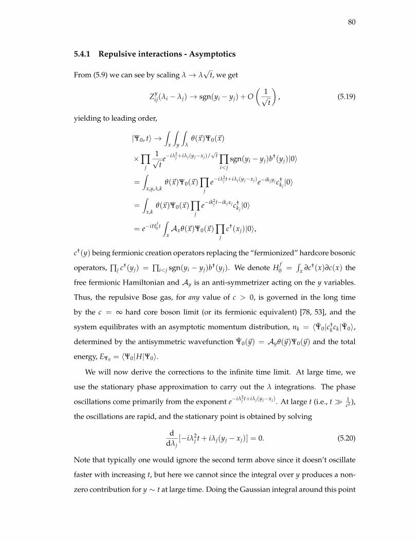
80
5.4.1 Repulsive interactions - Asymptotics
From (5.9) we can see by scaling λ → λ√t, we get
Zyij(λi − λj) → sgn(yi − yj) +O
(
1√t
)
, (5.19)
yielding to leading order,
|Ψ0, t〉 →∫
x
∫
y
∫
λθ(~x)Ψ0(~x)
× ∏j
1√te−iλ2
j+iλj(yj−xj)/√t∏i<j
sgn(yi − yj)b†(yj)|0〉
=∫
x,y,λ,kθ(~x)Ψ0(~x)∏
j
e−iλ2j t+iλj(yj−xj)e−ikjyjc†kj |0〉
=∫
x,kθ(~x)Ψ0(~x)∏
j
e−ik2j t−ikjxjc†kj |0〉
= e−iHf0 t∫
xAxθ(~x)Ψ0(~x)∏
j
c†(xj)|0〉,
c†(y) being fermionic creation operators replacing the “fermionized” hardcore bosonic
operators, ∏j c†(yj) = ∏i<j sgn(yi − yj)b
†(yj). We denote Hf0 =
∫
x ∂c†(x)∂c(x) the
free fermionic Hamiltonian and Ay is an anti-symmetrizer acting on the y variables.
Thus, the repulsive Bose gas, for any value of c > 0, is governed in the long time
by the c = ∞ hard core boson limit (or its fermionic equivalent) [78, 53], and the
system equilibrates with an asymptotic momentum distribution, nk = 〈Ψ0|c†kck|Ψ0〉,determined by the antisymmetric wavefunction Ψ0(~y) = Ayθ(~y)Ψ0(~y) and the total
energy, EΨ0= 〈Ψ0|H|Ψ0〉.
We will now derive the corrections to the infinite time limit. At large time, we
use the stationary phase approximation to carry out the λ integrations. The phase
oscillations come primarily from the exponent e−iλ2j t+iλj(yj−xj). At large t (i.e., t ≫ 1
c2),
the oscillations are rapid, and the stationary point is obtained by solving
d
dλj[−iλ2
j t+ iλj(yj − xj)] = 0. (5.20)
Note that typically one would ignore the second term above since it doesn’t oscillate
faster with increasing t, but here we cannot since the integral over y produces a non-
zero contribution for y ∼ t at large time. Doing the Gaussian integral around this point

81
(and fixing the S-matrix prefactor to its stationary value), we obtain for the repulsive
case,
|~x, t〉 →∫
y∏i<j
Zyij
(
yi − yj − xi + xj
2t
)
× ∏j
1√4πit
e−i(yj−xj)
2
4t +i(yj−xj)
2
2t b†(yj)|0〉. (5.21)
In the above expression, the wavefunction has support mainly from regions where
yj/t is of order one. In an experimental setup, one typically starts with a local finite
density gas, i.e., a finite number of particles localized over a finite length. With this
condition, at long time, we can neglect xj/t in comparison with yj/t, giving
|~x, t〉 →∫
y∏i<j
Zij(ξi − ξ j)∏j
1√4πit
eitξ2j−iξ jxjb†(yj)|0〉 (5.22)
where ξ = y2t .
We turn now to calculated the asymptotic evolution of some observables. To com-
pute the expectation value of the density we start from the coordinate basis states,
〈~x′, t|ρ(z)|~x, t〉 which we then integrate with the chosen initial state,
〈~x′, t|ρ(z)|~x, t〉 = ∑P
∫
y
(
∑j
δ(yj − z)
)
× ∏i<j
Zij(ξi − ξ j)Z∗PiPj
(ξPi − ξPj)∏j
1
4πte−i(ξ jxj−ξPj x
′j) (5.23)
Note that the above product of S-matrices is actually independent of the ordering
of the y. First, only those terms appear in the product for which the permutation P has
an inversion. For example, say for three particles, if P = 312, then the inversions are
13 and 23. It is only these terms which give a non-trivial S-matrix contribution. For
the non-inverted terms, here 12, we get
ξ1 − ξ2 − ic sgn(y1 − y2)
ξ1 − ξ2 − ic
ξ1 − ξ2 + ic sgn(y1 − y2)
ξ1 − ξ2 + ic(5.24)
which is always unity irrespective of the ordering of y1, y2. For a term with an inver-
sion, say 23, we get,
ξ2 − ξ3 − ic sgn(y2 − y3)
ξ2 − ξ3 − ic
ξ3 − ξ2 + ic sgn(y3 − y2)
ξ3 − ξ2 + ic(5.25)
which is always equal to
ξ2 − ξ3 + ic
ξ2 − ξ3 − ic≡ S(ξ2 − ξ3) (5.26)

82
irrespective of the sign of y2 − y3. This allows us to carry out the integration over the
yj.
Lattice initial state
In order to calculate physical observables, we have to choose initial states. We choose
two different initial states for the problem, one with N particles distributed with uni-
form density in a series of harmonic traps given by,
|Ψlatt〉 =∫
x
N
∏j=1
1
(πσ2)14
e− (xj+(j−1)a)2
2σ2 b†(xj)|0〉, (5.27)
such that the overlap between the wave functions of two neighboring particles is neg-
ligible. In this particular case, the ordering of the particles is induced by the limited
non-overlapping support of the wave function.
In the lattice-like state, the initial wave function starts out with the neighboring
particles having negligible overlap. At small time (as seen from (5.14)), the particle
repel each other, but they never cross due to the repulsive interaction. So at large
time, the interaction does not play a role since the wave functions are sufficiently non-
overlapping. It is only the P = 1 contribution then that survives, and we get for the
density
〈~x′, t|ρ(z)|~x, t〉 = ∑j
∏k 6=j
δ(xk − x′k)e−i z
2t (xj−x′j)
4πt. (5.28)
We need to integrate the position basis vectors |~x〉 over some initial condition. We do
this here for the lattice state (5.27) This gives
〈Ψlatt, t|ρ(z)|Ψlatt, t〉 = ρlatt(ξz) =Nσ
2√
πte− ξ2z
σ2 (5.29)
Mathematically, any S-matrix factor that appears will necessarily have zero contri-
bution from the pole - this is easy to see from the pole structure, and the ordering of the
coordinates. In order to get a non-zero result, we need to fix at least two integration
variables (i.e., the yj). Thus the first non-trivial contribution comes from the two-point
correlation function.
We now proceed to calculate the evolution of the noise, i.e., the two body cor-
relation function ρ2(z, z′; t)latt = 〈Ψlatt, t|ρ(z)ρ(z′)|Ψlatt, t〉. The contributions can be

83
grouped in terms of number of crossings, which corresponds to a grouping in terms
of the coefficient e−ca [90]. The leading order term can be explicitly evaluated and we
show below which terms contribute. In general we have
ρ2 latt(z, z′; t) = ∑
P
∫
y
(
∑j,K
δ(yj − z)δ(yk − z′)
)
× ∏i<j,(ij)∈P
S(ξi − ξ j)∏j
1
4πte−i(ξ jxj−ξPj x
′j). (5.30)
The above shorthand in the S-matrix product means that only the (ij) that belong to
the inversions in P are included. We will now determine which terms contribute in
this sum. First note that for integration over a particular ξ j, the residue depends on
the sign of xj − xPj . Let us consider a specific example. Consider the three particle case
with the term P = 321. All three S-matrix factors appear in this term. ξ3 has a pole at
ξ1− ic and ξ2− ic. Thus integrating over y3 will give a non-zero residue only if x3 > x′1
which is however not satisfied by the initial conditions we choose. So, everything is
zero, unless we do not integrate over y3, implying it has to be one of the measured
variables. Similarly for ξ1, the poles are at ξ2 + ic and ξ3 + ic. In order to get a non-
zero residue we need x1 < x′3 which again is not satisfied by the initial conditions. We
get a non-zero result if we pin ξ1. As for ξ2 it has poles both above and below the real
line and so this always gives a non-zero contribution irrespective of the sign of x2− x′2.
One can see that this argument can be extended to the case with more particles.
Depending on what coordinates we are measuring at, we’ll get a specific contribution
from the sum over permutations. The next simplification comes from not allowing
any crossings among the unmeasured coordinates. It can be shown that allowing for
these gives us a higher order contribution in e−ca. In other words, the leading order
contribution comes from terms such as P = 21, 32, 321, 4231, 5342, 52341, . . .. The only
exchanges are on the ends. A general term will therefore look like (for l < k),
∫
yδ(yl − z)δ(yk − z′) ∏
j 6=l,kS(ξi − ξ j)S(ξ j − ξk)
× e−iξ j(xj−x′j)
4πt
ξl − ξk + ic
ξl − ξk − ic
e−iξl(xl−x′k)−iξk(xk−x′l)
(4πt)2
(5.31)

84
We have to sum over l, k, which will automatically sum over the number of interme-
diate j’s appearing. We’ll integrate the above general term, since the yj integrals factor
anyway. This gives
∏i 6=k,l,j
δ(xi − x′i)S(ξl − ξk)e−iξl(xl−x′k)−iξk(xk−x′l)
(4πt)2
× ∏j
[
δ(xj − x′j)− S(ξl − ξk − ic)
×
θ(xj > x′j)e−i(ξl−ic)(xj−x′j)+
+ θ(xj < x′j)e−i(ξk+ic)(xj−x′j)
]
(5.32)
We can sum the different contributions now. Note that the number of terms appearing
the product over j is given by k− l − 1. So for a given l, we have to sum over all the k.
Using a shorthand notation, the sum can be written as (note that it is understood that
yl and yk are integrated over using the delta functions. We retain the indices to keep
track of the terms. We actually have ξl = 2zt and ξk = 2z′t.
∑l,k
∏i<l,i>k
δi flk
k−1
∏j=l+1
gjlk (5.33)
In order to proceed with the summation, we have to integrate over the x. We use the
initial conditions described by (5.27), i.e., the lattice-like state. We’ll do it term by term.
∫
xi ,x′i
δ(xi − x′i)e− (xi+(i−1)a)2
2σ2− (x′
i+(i−1)a)2
2σ2√πσ2
= 1 (5.34)
∫
xl ,x′k ,xk ,x
′l
flke−∑l,k,l′ ,k′
(xl+(l−1)a)2
2σ2
πσ2
=σ2
4πt2S(ξl − ξk)e
−(ξ2l +ξ2k )σ2eia(k−l)(ξk−ξl) (5.35)
∫
xj,x′j
gjlke− (xj+(j−1)a)2
2σ2−
(x′j+(j−1)a)2
2σ2
πσ2= 1− 2c
√πσ
× S(ξl − ξk − ic)[
e(c+iξl)2σ2
erfc(c+ iξl)σ+
+ e(c−iξk)2σ2
erfc(c− iξk)σ]
(5.36)

85
Note that last expression has no j dependence. So, the sum over the product over j is
just a geometric series. Recall that ξl and ξk are fixed at z and z′ respectively. This series
can be summed. Note that the number of terms in the product is equal to the k − l,
and summing over them is effectively summing over k. The previous term therefore
needs to be taken into account. Writing ξl = ξz and ξk = ξz′ , we can write the sum as
σ2
4πt2S(ξz − ξz′)e
−(ξ2x+ξ2z′ )σ
2
∑l<k
eia(k−l)(ξz−ξz′ )gk−l−1zz′ (5.37)
where
gzz′ = 1− 2c√
πσS(ξz − ξz′ − ic)[
e(c+iξz)2σ2erfc(c+ iξz)σ+
+ e(c−iξz′ )2σ2
erfc(c− iξz′)σ]
(5.38)
Finally, we have to account for the k > l case which is equivalent to setting ξl = ξz′
and ξl = ξz. Doing this is further equivalent to adding the complex conjugate. We also
have to take into account the term with no permutations. So, finally we have,
ρ2 latt(z, z′) =
N2σ2
4πt2e−(ξ2x+ξ2
z′ )σ2
[
1+2
N2ReS(ξz − ξz′)
× eia(z−z′)N(1− eia(z−z′)g) + eiaN(z−z′)gNzz′ − 1
[1− gzz′eia(z−z′)]2
]
(5.39)
To compare with the Hanbury-Brown Twiss result, we calculate the normalized spatial
noise correlations, given by C2(z, z′) ≡ ρ2(z,z′)
ρ(z)ρ(z′) − 1 ≡ C2(z, z′). In the non-interacting
case, i.e., c = 0, S(ξ) = 1 and gzz′ = 0 and we recover the HBT result for N = 2,
C02(ξz, ξz′) =
1
2cos(a(ξz − ξ ′z)) (5.40)
One can also check that the limit of c → ∞ gives the expected answer for free fermions,
namely,
C∞2 (ξz, ξz′) = −1
2cos(a(ξz − ξ ′z)) (5.41)
At finite cwe can see a sharp fermionic character appear that broadens with increasing
c as shown in Fig. 5.7. The large time behavior is captured in a small window around
ξ = 0. One can see that at any finite c, the region near zero develops a strong fermionic
character, thus indicating that irrespective of the value of the coupling that we start

86
- 2 - 1 1 2Ξa
- 0.4
- 0.2
0.2
0.4
C2 H Ξ , - Ξ L
¥
10
5
2
1.2
0.8
0.4
0.2
0
Figure 5.7: Normalized noise correlation function C2(ξ,−ξ). Fermionic correlationsdevelop on a time scale τ ∼ c−2, so that for any c we get a sharp fermionic peak nearξ = 0, i.e., at large time. The key shows values of ca .
with, the model flows towards an infinitely repulsive model at large time, that can be
described in terms of free fermions. We also obtained this result “at” t = ∞ at the
beginning of this section.
For higher particle number, we see “interference fringes” corresponding to the
number of particles, that get narrower and more numerous with an increase, mem-
ory of the initial lattice state. However, the asymptotic fermionic character does not
disappear. Figures 5.8 and 5.9 show the noise correlation function for five and ten par-
ticles respectively. The large peaks are interspersed by smaller peaks and so on. This
reflects the character of the initial state.
- 20 - 10 10 20Ξa
- 0.5
0.5
1.0
C2 H Ξ , - Ξ L
Figure 5.8: Normalized noise correlation function for five particles released for a Mott-like state for c > 0

87
- 20 - 10 10 20Ξa
- 2
- 1
1
2
3
C2 H Ξ , - Ξ L
Figure 5.9: Normalized noise correlation function for ten particles released for a Mott-like state for c > 0.
Quenching from a bound state
In this section our initial state is the ground state of the attractive Lieb-Liniger Hamil-
tonian (with interaction strength −c0 < 0. For two bosons, this take the form [94],
|Ψbound〉 =∫
~xe−c0|x1−x2|−
x212σ2
− x222σ2 b†(x1)b
†(x2)|0〉, (5.42)
and we quench it with a repulsive Hamiltonian.The long time noise correlations are
displayed in Fig. 5.10. We see that while the initial state correlations are preserved over
most of the evolution, in the asymptotic long time limit the characteristic fermionic
dip. We expect similar effects for any number of bosons.
- 10 - 5 5 10Ξ
- 1.0
- 0.5
0.5
1.0
C2 H Ξ , - Ξ L
3
1
0
Figure 5.10: Normalized noise correlation function for two particle quenched from abound state into the repulsive regime. The legend indicates the values of c that thestate is quenched into. We start with c0σ2 = 3, σ = 1, c0 being the interaction strengthof the initial state Hamiltonian. Again, we see the fermionic dip, but the rest of thestructure is determined by the initial state.

88
5.4.2 Attractive interactions
For the attractive case, since the contours of integration are spread out in the imaginary
direction, we have the contributions from the poles in addition to the stationary phase
contributions at large time. The stationary phase contribution is picked up on the
real line, but as we move the contour, it stays pinned above the poles and we need
to include the residue obtained from going around them, leading to sum over several
terms.Fig. 5.11 shows an example of how this works.
> |c|
Figure 5.11: Contribution from stationary phase and pole at large time in the attractivemodel. The blue (lower) contour represents the shifted contour.
In Ref. [71], a formula was provided for the asymptotic state. Here we give a more
careful treatment by taking into account that the fixed point of the approximation
moves for terms that come from a pole of the S-matrix. It is therefore necessary to
first shift the contours of integration, and then carry out the integral at long time. We
carry this out below.
Shifting a contour over a pole leads to an additional term from the residue:
∫
γ2
dλ2
2π→∫
γR2
dλ2
2π− iR(λ2 → λ1 + i|c|) (5.43)
where R(x) indicates that we evaluate the residue given by the pole x. γj indicates
the original contour of integration and γRj indicates that integration is carried out over
the real axis. Proceeding with the other variables we end up with
∫
γ1,γ2,··· ,γN
→∫
γR1
[
∫
γR2
+iR(λ2 → λ1 + i|c|)]
×[
∫
γR3
+iR(λ3 → λ1 + i|c|) + iR(λ3 → λ2 + i|c|)]
· · ·
×[
∫
γRN
+iR(λN → λ1 + i|c|) + iR(λN → λ2 + i|c|)+
+ · · ·+ iR(λN → λN−1 + i|c|)]
(5.44)

89
The integrals can now be evaluated using the stationary phase approximation. The
correction produced by the above procedure does not affect the qualitative features
observed in Ref. [71].
Lattice initial state
We now calculate the evolution of the density and the two body correlation function
in order to compare with the repulsive case. We will first study the two particle case.
Although we have a finite time expression for this case from which we can directly
take a long time limit, we will study the asymptotics using the above scheme for an
N-particle state, since we have an analytical expression to go with. We get two terms,
the first being the stationary phase contribution, and is just like the repulsive case
with c → −c. The second is the contribution from the pole. It contains the bound
state contribution which brings about another interesting feature of the attractive case.
While the asymptotic dynamics of the repulsive model is solely dictated by the new
variables ξ j ≡ yj2t , and all the time dependence of the wave function enters through
this “velocity” variable, this is not the case in the attractive model. While it is true that
the system is naturally described in terms of ξ variables, there still exists non-trivial
time dependence.
First, we integrate out the x dependence assuming an initial lattice-like state. This
gives,
|Ψlatt(t)〉 =∫
y∑
ξ∗j =ξ j,ξ∗i +ic,i<j
∏i<j
Sij(ξ∗i − ξ∗j )∏
j
(4πσ2)14√
4πit
× e−(σ2/2+it)(ξ∗j )2+iξ∗j (2tξ j+a(j−1))b†(yj)|0〉. (5.45)
Defining φ(ξ, t) from |Ψlatt(t)〉 =∫
y φ(ξ, t)∏j b†(yj)|0〉, we have for the density evolu-
tion under attractive interactions, c < 0,
ρ−latt(z; t) = ∑P,j
∫
yδ(yj − z)φ∗(ξP, t)φ(ξ, t) (5.46)
We can show numerically (the expressions are a bit unwieldy to write here), that
asymptotically, the density shows the same Gaussian profile that we expect from a
uniformly diffusing gas, namely, e−ξ2σ2.

90
With this, we can proceed to compute the noise correlation function. The two par-
ticle case is easy, as there are no more integrations to carry out. We get,
ρ−2 latt(z, z′; t) = ∑
P,j,k
∫
yδ(yj − z)δ(yk − z′)φ∗(ξP, t)φ(ξ, t)
= |φs(ξz, ξ′z)|2,
(5.47)
where φs is the symmetrized wavefunction. Fig.5.12 shows the normalized noise cor-
relations for different values of t.
- 6 - 4 - 2 2 4 6Ξ a
0.1
0.2
0.3
0.4
C2 H Ξ , - Ξ L t
Figure 5.12: Variation of C2 for the attractive case with time. Note the growth of thecentral peak. At larger times, the correlations away from zero fall off. ta2 = 20, 40, 60for blue (top), magenta (middle) and yellow (bottom) respectively.
For more particles, we see interference fringes similar to the repulsive case. We
note that the central peak increases and sharpens with time, indicating increasing con-
tribution from bound states to the correlations (see Fig. 5.13 for an example).
5.4.3 Starting with a condensate - attractive and repulsive interactions
In this section, we study the evolution of the Bose gas after a quench from an initial
state where all the bosons are in a single level of a harmonic trap. For t < 0, the state
is described by
|Ψcond〉 =∫
xSx ∏
j
e−
x2j
σ2
(πσ2)14
b†(xj)|0〉. (5.48)
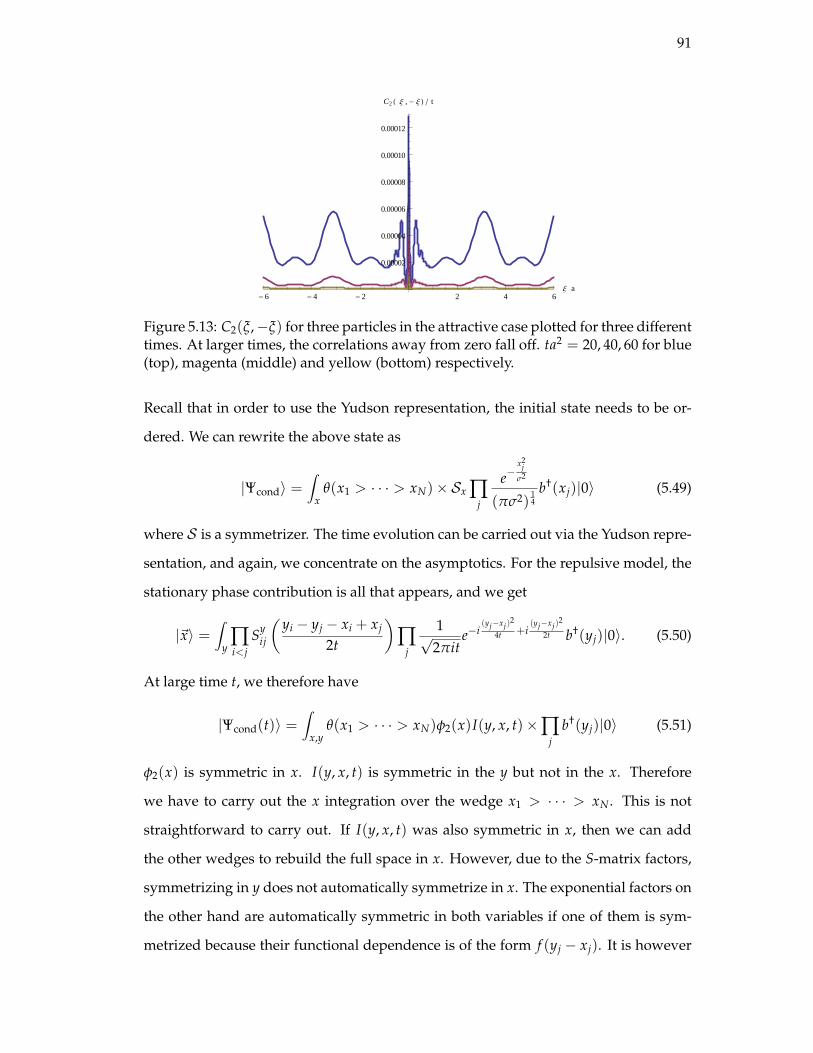
91
- 6 - 4 - 2 2 4 6Ξ a
0.00002
0.00004
0.00006
0.00008
0.00010
0.00012
C2 H Ξ , - Ξ L t
Figure 5.13: C2(ξ,−ξ) for three particles in the attractive case plotted for three differenttimes. At larger times, the correlations away from zero fall off. ta2 = 20, 40, 60 for blue(top), magenta (middle) and yellow (bottom) respectively.
Recall that in order to use the Yudson representation, the initial state needs to be or-
dered. We can rewrite the above state as
|Ψcond〉 =∫
xθ(x1 > · · · > xN)× Sx ∏
j
e−
x2j
σ2
(πσ2)14
b†(xj)|0〉 (5.49)
where S is a symmetrizer. The time evolution can be carried out via the Yudson repre-
sentation, and again, we concentrate on the asymptotics. For the repulsive model, the
stationary phase contribution is all that appears, and we get
|~x〉 =∫
y∏i<j
Syij
(
yi − yj − xi + xj
2t
)
∏j
1√2πit
e−i(yj−xj)
2
4t +i(yj−xj)
2
2t b†(yj)|0〉. (5.50)
At large time t, we therefore have
|Ψcond(t)〉 =∫
x,yθ(x1 > · · · > xN)φ2(x)I(y, x, t)× ∏
j
b†(yj)|0〉 (5.51)
φ2(x) is symmetric in x. I(y, x, t) is symmetric in the y but not in the x. Therefore
we have to carry out the x integration over the wedge x1 > · · · > xN . This is not
straightforward to carry out. If I(y, x, t) was also symmetric in x, then we can add
the other wedges to rebuild the full space in x. However, due to the S-matrix factors,
symmetrizing in y does not automatically symmetrize in x. The exponential factors on
the other hand are automatically symmetric in both variables if one of them is sym-
metrized because their functional dependence is of the form f (yj − xj). It is however
92
possible to make the S-matrix factors approximately symmetric in x, and we will de-
fine what we mean by approximately shortly. What is important is to obtain a yj − xj
dependence. As of now, the S-matrix that appears in the above expression is
Syij
(
yi − yj − xi + xj
2t
)
=
yi−yj−xi+xj2t − ic sgn(yi − yj)
yi−yj−xi+xj2t − ic
(5.52)
First, we can change sgn(yi − yj) to sgn(
yi−yj2t
)
since t > 0. Next, note that asymp-
totically in time, the stationary phase contribution comes fromy2t ∼ O(1). However,
since x has finite extent, at large enough time, x2t ∼ 0. We are therefore justified in
writing sgn(
yi−xi2t − yj−xj
2t
)
. The only problem could arise when yi ∼ yj. However, if
this occurs, then the S-matrix is approximately sgn(yi − yj) which is antisymmetric in
ij. With this prefactor the particles are effectively fermions, and therefore at yi ∼ yj,
the wave-function has an approximate node. At large time therefore, we do not have
to be concerned with the possibility of particles overlapping, and including the xi in-
side the sgn function is valid. With this change the S-matrix also becomes a function
of yj − xj and symmetrizing over y one automatically symmetrizes over x.
In short, we have established that the wave function asymptotically in time can be
made symmetric in x. This allows us to rebuild the full space. We get
|Ψcond(t)〉 =∫
x,y∑P
θ(xP)φ2(x)Is(y, x, t)∏
j
b†(yj)|0〉
=∫
x,yφ2(x)I
s(y, x, t)∏j
b†(yj)|0〉(5.53)
where the s superscript indicates that we have established that I(y, x, t) is also sym-
metric in x. With this in mind, we can do away with the ordering when we’re inte-
grating over the x if we symmetrize the initial state wave function and the final wave
function. Note that when we calculate the expectation value of a physical observable,
the symmetry of the wavefunction is automatically enforced, and thus taken care of
automatically.
Recall that when we calculated the noise correlations of the repulsive gas, in order
to get an analytic expression for N particles, we considered the leading order term,
i.e., the HBT term. We did this by showing that higher order crossings produced terms
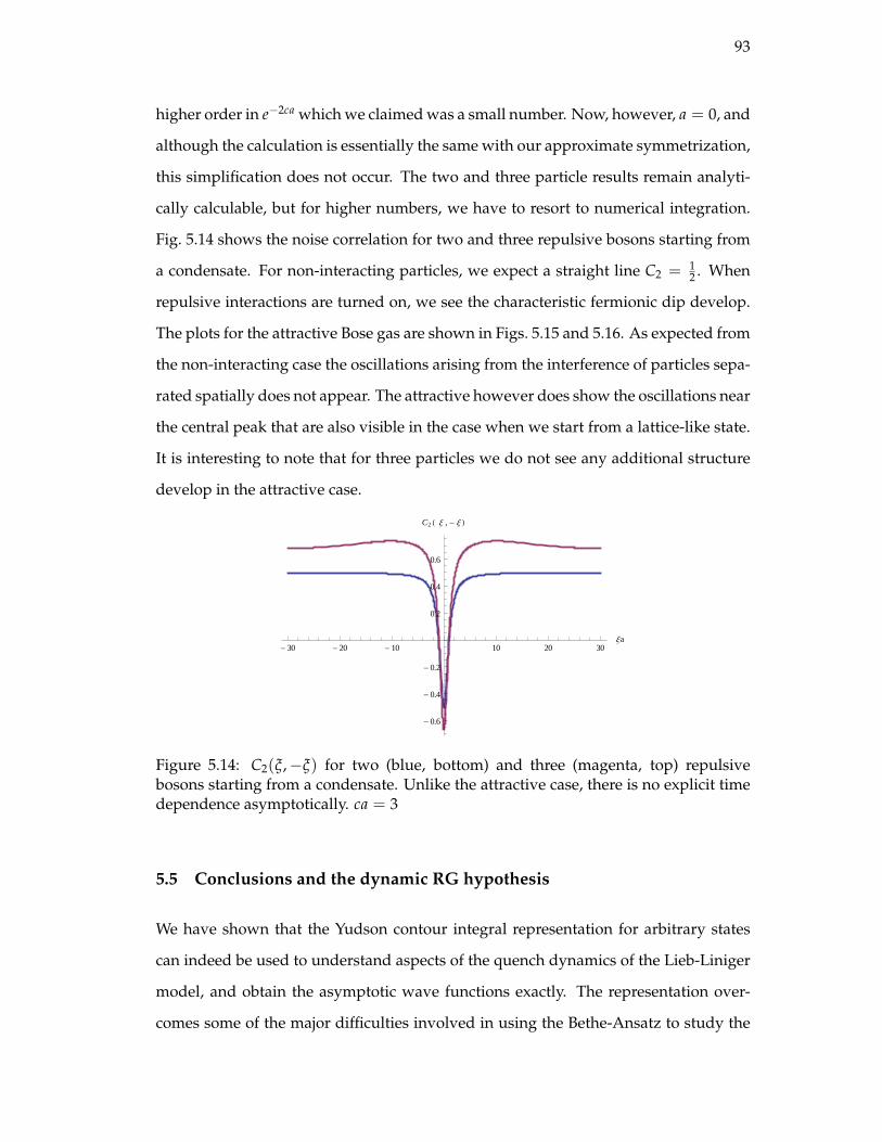
93
higher order in e−2ca whichwe claimedwas a small number. Now, however, a = 0, and
although the calculation is essentially the same with our approximate symmetrization,
this simplification does not occur. The two and three particle results remain analyti-
cally calculable, but for higher numbers, we have to resort to numerical integration.
Fig. 5.14 shows the noise correlation for two and three repulsive bosons starting from
a condensate. For non-interacting particles, we expect a straight line C2 = 12 . When
repulsive interactions are turned on, we see the characteristic fermionic dip develop.
The plots for the attractive Bose gas are shown in Figs. 5.15 and 5.16. As expected from
the non-interacting case the oscillations arising from the interference of particles sepa-
rated spatially does not appear. The attractive however does show the oscillations near
the central peak that are also visible in the case when we start from a lattice-like state.
It is interesting to note that for three particles we do not see any additional structure
develop in the attractive case.
- 30 - 20 - 10 10 20 30Ξa
- 0.6
- 0.4
- 0.2
0.2
0.4
0.6
C2 H Ξ , - Ξ L
Figure 5.14: C2(ξ,−ξ) for two (blue, bottom) and three (magenta, top) repulsivebosons starting from a condensate. Unlike the attractive case, there is no explicit timedependence asymptotically. ca = 3
5.5 Conclusions and the dynamic RG hypothesis
We have shown that the Yudson contour integral representation for arbitrary states
can indeed be used to understand aspects of the quench dynamics of the Lieb-Liniger
model, and obtain the asymptotic wave functions exactly. The representation over-
comes some of the major difficulties involved in using the Bethe-Ansatz to study the

94
- 1.0 - 0.5 0.5 1.0Ξ a
0.1
0.2
0.3
0.4
0.5
C2 H Ξ , - Ξ L t
Figure 5.15: Noise correlation for two attractive bosons starting from a condensate - astime increases from blue (top) to yellow (bottom), the central peak dominates.
- 2 - 1 1 2Ξ a
0.0002
0.0004
0.0006
0.0008
C2 H Ξ , - Ξ L t
Figure 5.16: C2(ξ,−ξ) for three attractive bosons starting from a condensate. Note thatthe side peak structure found in fig. 5.13 is missing due to the initial condition. Weshow the evolution at three times. As time increases, the oscillations near the centralpeak die out. Times from top to bottom tc2 = 20, 40, 60.
dynamics of some integrable systems by automatically accounting for complicated
states in the spectrum.
We see some interesting dynamical effects at long times. The infinite time limit of
the repulsive model corresponds to particles evolving with a free fermionic Hamilto-
nian. It retains, however, memory of the initial state and therefore is not a thermal
state. The correlation functions approach that of hard core bosons at long time indi-
cating a dynamical increase in interaction strength. The attractive model also shows
a dynamic strengthening of the interaction and the long time limit is dominated by a
multiparticle bound state. This of course does not mean that it condenses. In fact the

95
state diffuses over time, but remains strongly correlated.
We may interpret our results in terms of a “dynamic RG” in time. The asymptotic
evolutions of the model both for c > 0 and for c < 0 are given by the Hamiltonians H∗±
with c → ±∞ respectively. Accepting the RG logic behind the conjecture one would
expect that there would be basins of attraction around the Lieb-Liniger Hamiltonian
with models whose long time evolution would bring them close to the ”dynamic fixed
points” H∗±. One such Hamiltonian would have short range potentials replacing the
δ-function interaction that renders the Lieb-Liniger model integrable. Perhaps, lattice
models could be also found in this basin whose time asymptotics would be close, in
the repulsive case, to that given by a free fermionic model on the lattice. Clearly, as
discussed earlier, the Bose-Hubbard model is not such a model since it has a lattice
symmetry that is not present in the Lieb-Liniger model. This could be however over-
come by adding such terms as the next nearest hopping or interactions that break this
symmetry, or as shown in Appendix A, with an appropriate choice of initial state.
We have to emphasize, however, that as these models are not integrable, we do
not expect that they would actually flow to H∗±. Instead, starting close enough in
the “basin”, they would flow close to H∗± and spend much time in its neighborhood,
eventually evolving into another, thermal state. We thus conjecture that away from
integrability, a system would approach the corresponding non-thermal equilibrium,
where the dynamics will slow down leading to a “prethermal” state [10]. Fig. 5.17
shows a schematic of this. Such prethermalization behavior has indeed been observed
in lattice models [85]. The system is expected to eventually find a thermal state. It
is therefore of interest to characterize different ways of breaking integrability to see
when a system is “too far” from integrability to see this effect and in what regimes a
system can be considered as close to integrability. For a review and background on
this subject, see Ref. [112].
Further, the flow diagram in Fig. 5.17 might have another axis that represents ini-
tial states. Studying the Bose-Hubbard model shows an interesting initial state depen-
dence. Whereas the sign of the interaction does not affect the quench dynamics, the
asymptotic state depends strongly on the initial state, with a lattice-like state leading to

96
fermionization, and a condensate-like state retaining bosonic correlations. The strong
dependence on the initial state in the quench dynamics is evident from eq. (2.11) and
is subject of much debate, in particular as relating to the Eigenstate Thermalization
Hypothesis [117, 130, 39].
c = −∞ c = 0 c = ∞
thermal state
pre-thermalization
non-integrable model
Figure 5.17: Schematic showing pre-thermalization of states in a non-integrable model
This work also opens up several new questions. It provides a prediction for exper-
iments that can be carried out in the context of continuum cold atom systems (though
the experiments we are aware of are carried out on the lattice and therefore described
by the Bose-Hubbard model) Theoretically, while the representation is provable math-
ematically, further investigation is required to understand, physically, how it achieves
the tedious sum over eigenstates, while automatically accounting for the details of the
spectrum. This would allow us to extend the approach to other models with a more
complicated S-matrix structure. It would also be useful to tie this approach to other
means of calculating overlaps in the Algebraic Bethe Ansatz, i.e., the form-factor ap-
proach. The representation can essentially be thought of as a different way of writing
the identity operator. From that standpoint, it could serve as a new way of evaluating
correlation functions using the Bethe Ansatz. We are currently studying generaliza-
tions of this approach to other models that can be realized in optical lattices.

97
Chapter 6
Quench dynamics of the Heisenberg chain
In this Chapter, we show some preliminary results regarding the quench dynamics of
the isotropic Heisenberg chain, or the XXX model. We’ll start with the noninteracting
version, the XX model and try to understand the time evolution of the spin current
starting from a domain wall state. Before we do that, we’ll work out the Yudson rep-
resentation for the Heisenberg model, starting with the noninteracting case of the XX
model.
6.1 XX model
We’ll start with the XX Heisenberg chain in one dimension. The Hamiltonian is
H = −JM
∑j=−M
σxj σx
j+1 + σyj σ
yj+1 (6.1)
It describes spins hopping on a lattice of M sites. We will take M to be very large, and
consequently, will not worry about the boundary conditions at this point. Our goal is
to work in an open system. The above model is non-interacting since there is no σz
term. The eigenstates can be written by inspection:
|k〉 = ∑P
M
∑mi=−M
N
∏j=1
eikPjmjσ−
mj|0〉 (6.2)
where k j are the momenta, and the vacuum state |0〉 is defined as the state with all
spins up, i.e., σ+j |0〉 = 0. Acting on the above state with the Hamiltonian (6.1), we get,
H|k〉 = −2J ∑P
∑mi
∑l
∏j 6=l
eikPjmj+ikPlml (σ−
ml+1 + σ−ml−1)σ
−mj|0〉
= −2J ∑P
∑mi
∑l
∏j
eikPjmj2 cos(kPl )σ
−mj|0〉 = −4J
(
∑l
cos kl
)
|k〉.(6.3)

98
The energy eigenvalues are given by
E = −4JN
∑j=1
cos k j, k ∈ [−π,π]. (6.4)
The spin of the above state,
Sz =M
2− N, N ≤ M. (6.5)
The above can also be alternatively be carried out in the language of fermions us-
ing the Jordan-Wigner transformation. We will however, stick to the spin operator
notation.
6.1.1 The Yudson representation in the natural parametrization
We are interested in a Yudson-like integral representation for an arbitrary state. Let’s
say we start with a state that has N spins flipped. A general state can be written as,
|Ψ0〉 =N
∏j=1
σ−nj|0〉. (6.6)
We can also assume without loss of generality that n1 > n2 > · · · > nN . Our goal is to
show that
|Ψ0〉 =∫
kj|~k〉(~k|Ψ0〉, (6.7)
where we are yet to determine the meaning of the “Yudson state” |~k) and the contours
of integration. Given that this is a non-interacting model, these are fairly obvious. We
chose
|~k) = ∑mi
θ(m1 > · · · > mN)N
∏j=1
eikjmjσ−mj|0〉 (6.8)
and integrate all the k j from [−π,π]. We get,
|Ψ0〉 = ∑mi
N
∏j=1
∫ π
−π
dk j
2πeikj(mj−nj)σ−
mj|0〉
= ∑mi
N
∏j=1
sin[π(mj − nj)]
π(mj − nj)σ−mj|0〉.
(6.9)
Since mj − nj is an integer, the above function is zero unless mj = nj for all j, thus
proving the claim. We can now carry out the time evolution by acting on it with e−iHt.

99
The finite time state is given by,
|Ψ(t)〉 = ∑mi
N
∏j=1
∫ π
−π
dk j
2πe4iJt cos kjeikj(mj−nj)σ−
mj|0〉
= ∑mi
∏j
JBmj−nj(−4Jt)σ−
mj|0〉.
(6.10)
where JBn is the Bessel function of the first kind. The expectation value of the spin at
some site m, e.g., evolves as
〈σzm〉 = 〈Ψ(t)|σz
m|Ψ(t)〉
= ∑mi ,m
′i
∏j
JBmj−nj(−4Jt)JBm′
j−nj(−4Jt)〈0|σ+
m′jσzmσ−
mj|0〉
= ∑mi ,m
′i
∏j
JBmj−nj(−4Jt)JBm′
j−nj(−4Jt)(1− 2δm,mj
)〈0|σ+m′
jσ−mj|0〉
= ∑P
∑mi
∏j
JBmj−nj(−4Jt)JBmPj
−nj(−4Jt)(1− 2δm,mj
)
= ∑P
∑mi
∏j
JBmj−nj(−4Jt)JBmj−nPj
(−4Jt)(1− 2δm,mj).
(6.11)
6.1.2 The λ parametrization
We’ll also work out the above in another parametrization of the momentum. In view
of having eventually to deal with the XXXmodel, we will reparametrize the momenta
in terms of rapidities,
k = 2 tan−1 2λ. (6.12)
For k ∈ [−π,π], λ ∈ [−∞,∞]. The energy becomes
E = −4J ∑j
cos k j = −2J ∑j
(
1
(λ2j +
14 )
− 2
)
. (6.13)
We can always shift the energies to eliminate the constant term. The measure of the
integral in the Yudson representation transforms as well:
dk → dλ
λ2 + 14
(6.14)
and λ ∈ [−∞,∞]. In this language, the Yudson representation becomes
|Ψ0〉 = ∑yi
∏j
∫ ∞
−∞
dλj
2π(λ2j +
14 )
ei2 tan−1(2λj)(mj−nj)σ−
mj|0〉
= ∑yi
∏j
∫ ∞
−∞
dλj
2π(λ2j + 1/4)
(
−λj − i/2
λj + i/2
)mj−nj
σ−mj|0〉.
(6.15)

100
Our reparametrization has therefore introduced a new analytic structure on the inte-
grand. The measure now has poles as ±i. The integrand has poles at +i/2 or −i/2
depending on whether m > or < n. Since in this simple case, the integrand factorizes,
let us consider the j-th integral. If mj > nj, then the integrand has a pole (in general,
multiple, but no branch-cuts) at λj = −i/2. We want to avoid this pole since it is a
multiple pole. In order to carry out the integral we are allowed to close the contour
in either the upper or the lower half plane and use the residue theorem. We choose
to close the contour in the upper half plane picking up the pole at λj = i/2 coming
from the measure. However, the integrand vanishes at λj = i/2, and so we must have
mj ≤ nj. For mj < nj, the integrand has a pole at λj = i/2, and so to avoid it, we close
the contour in the lower half plane picking up the pole at−i/2 from the measure. But,
again, at −i/2, the integrand vanishes. So, we must have that mj = nj. In order to
calculate the value of the integral, we can use the residue theorem again. We have,
|Ψ0〉 = ∑yi
∏j
∫ ∞
−∞
dλj
2π(λ2j + 1/4)
δmj,njσ−mj|0〉
=N
∏j=1
θ(xj)σ−mj|0〉.
(6.16)
thus proving the identity.
At finite time, it might seem that the exponent is badly behaved at the poles, but a
straightforward series expansion of the exponent, followed by integration, and resum-
mation will give us the Bessel function obtained in the previous section. At any rate,
the fact that poles appear in the “plane wave” part of the wave function is unusual.
In Appendix B, we show how these poles physically correspond to hopping produced
by the time evolution.
One can show that after a long time evolution, the system becomes quadratic free
fermions, which is expected as the low-energy physics of fermions on a lattice: Ek ∼cos k = 1− k2
2 + . . ..
We will now shift our attention to understanding the ferromagnetic XXX model,
which has a non-trivial two particle S-matrix. The structure of the S-matrix will de-
termine the integration contours. We follow the description of this model provided
in [86].

101
6.1.3 Long time asymptotics
While we can obtain the finite time wavefunction explicitly in the free model, it is
instructive to study the asymptotic behavior directly in both the k and the λ languages.
In the k language, the integral we have is
∫
ke4iJt cos keik(m−n) (6.17)
At long time, we can do a stationary phase approximation:
d
dk[4iJt cos k+ ik(m− n)] = 0 =⇒ sin k =
m− n
4Jt. (6.18)
The value of the integral is therefore (up to prefactors)
exp
√
1−(
m− n
4Jt
)2
√
1−(
m− n
4Jt
)2
+ im− n
4Jt
. (6.19)
For the energy to be a real number, we require
∣
∣
∣
∣
m− n
4Jt
∣
∣
∣
∣
≤ 1 (6.20)
which is like a Lieb-Robinson [95] bound.
In the λ language, we have
∫
λe
2i Jt
(λ2+ 14)+i2 tan−1(2λ)(m−n)
(6.21)
The stationary phase approximation yields
d
dλ
[
2iJt
(λ2 + 14 )
+ i2 tan−1(2λ)(m− n)
]
=⇒ λ =1±
√
1−(
m−n4Jt
)2
(m− n)/2Jt. (6.22)
This also produces the same bound as above.
6.2 XXX model
The XXX Hamiltonian is given by
H = −J ∑j
(
σxj σx
j+1 + σyj σ
yj+1 + σz
j σzj+1 − 1
)
. (6.23)

102
The model has two vacua, one with all spins pointing up, and the other with all down.
We’ll use the “up” vacuum.
σ+j |0〉 ≡ 0. (6.24)
Also, we introduce the spin raising and lowering operators,
σ±j ≡
σxj ± iσ
yj
2. (6.25)
Their commutation relations are,
[σ+m , σ+
n ] = [σ−m , σ−
n ] = 0, [σ+m , σ−
n ] = σzmδmn, [σz
m, σ±n ] = ±2σ±
m δmn. (6.26)
Rewriting the Hamiltonian (6.23) using the above operators, we get,
H = −J ∑j
(
2(
σ−j σ+
j+1 + σ−j+1σ+
j
)
+ σzj σz
j+1 − 1)
. (6.27)
6.2.1 Eigenstates
The one particle eigenstates of this model are:
|λ1〉 = ∑m1
(
λ1 + i/2
λ1 − i/2
)m1
σ−m1|0〉. (6.28)
We can check this explicitly.
H|λ1〉 = −2J ∑m1
(
λ1 + i/2
λ1 − i/2
)m1
(σ−m1+1 + σ−
m1−1 − 2σ−m1)|0〉
= −2J ∑m1
(
λ1 + i/2
λ1 − i/2
)m1(
λ1 + i/2
λ1 − i/2+
λ1 − i/2
λ1 + i/2− 2
)
σ−m1|0〉
= −2J−1
λ21 +
14
|λ1〉.
(6.29)
So for one spin down, the energy is E(λ1) ≡ 2J
λ1+14
.
We now need the two particle eigenstates of this model. In what follows, we’ll
only check if the state below is a solution of the Schrodinger equation. This generally
follows the approach in [109].
|λ1,λ2〉 = ∑m1,m2
λ1 − λ2 − i sgn(m1 −m2)
λ1 − λ2 − i(
λ1 + i/2
λ1 − i/2
)m1(
λ2 + i/2
λ2 − i/2
)m2
σ−m1
σ−m2|0〉. (6.30)

103
m1 and m2 are summed over Z. It is important that we work on an infinite line, since
making it finite will necessitate the use of boundary conditions, which will constrain
the momenta. We will first consider the case when the two spins are not neighboring.
The sgn function in the S-matrix is not affected as the hopping cannot interchange
spins that aren’t neighboring. So,
H|λ1,λ2〉far = −2J ∑j
∑m1,m2
λ1 − λ2 − i sgn(m1 −m2)
λ1 − λ2 − i
(
λ1 + i/2
λ1 − i/2
)m1(
λ2 + i/2
λ2 − i/2
)m2
× (σ−j σ+
j+1 + σ−j+1σ+
j +1
2σzj σz
j+1)σ−m1
σ−m2|0〉
= −2J ∑m1,m2
λ1 − λ2 − i sgn(m1 −m2)
λ1 − λ2 − i
(
λ1 + i/2
λ1 − i/2
)m1(
λ2 + i/2
λ2 − i/2
)m2
× (σ−m1−1σ−
m2+ σ−
m1σ−m2+1 + σ−
m1+1σ−m2
+ σ−m1
σ−m2−1 − 4σ−
m1σ−m2)|0〉
= −2J ∑m1,m2
λ1 − λ2 − i sgn(m1 −m2)
λ1 − λ2 − i
(
λ1 + i/2
λ1 − i/2
)m1(
λ2 + i/2
λ2 − i/2
)m2
×(
λ1 + i/2
λ1 − i/2+
λ1 − i/2
λ1 + i/2+
λ2 + i/2
λ2 − i/2+
λ2 − i/2
λ2 + i/2− 4
)
σ−m1
σ−m2|0〉
= [E(λ1) + E(λ2)]|λ1,λ2〉far′ − 2J ∑m1,m2
λ1 − λ2 − i sgn(m1 −m2)
λ1 − λ2 − i
×(
λ1 + i/2
λ1 − i/2
)m1(
λ2 + i/2
λ2 − i/2
)m2[
δm1,m2+1λ1 + i/2
λ1 − i/2+
+ δm1+1,m2
λ1 − i/2
λ1 + i/2+ δm1+1,m2
λ2 + i/2
λ2 − i/2+
+ δm1,m2+1λ2 − i/2
λ2 + i/2
]
σ−m1
σ−m2|0〉.
(6.31)
In the above expression, “far” indicates that the next to nearest neighbor state that ap-
pears in it is incomplete. The remaining piece will come from the below state. We now
consider the case of two neighboring spins. This is the only case where the interaction

104
is active. The state we consider is,
|λ1,λ2〉near = ∑m1,m2
(δm1+1,m2+ δm1,m2+1)
λ1 − λ2 − i sgn(m1 −m2)
λ1 − λ2 − i
×(
λ1 + i/2
λ1 − i/2
)m1(
λ2 + i/2
λ2 − i/2
)m2
σ−m1
σ−m2|0〉
= ∑m1
(
λ1 + i/2
λ1 − i/2
)m1(
λ2 + i/2
λ2 − i/2
)m1[
λ1 − λ2 + i
λ1 − λ2 − i
λ2 + i/2
λ2 − i/2+
λ1 + i/2
λ1 − i/2
]
σ−m1
σ−m1+1|0〉
(6.32)
For two neighboring down spins, the kinetic terms can either put the spins on top
of each other, a process which is forbidden in the spin- 12 model, or it can separate the
spins by a single up spin. This changes the energy of the system. For antiferromagnetic
coupling, this decreases the energy.
H|λ1,λ2〉near
= −2J ∑j
∑m1,m2
(δm1+1,m2+ δm1,m2+1)
λ1 − λ2 − i sgn(m1 −m2)
λ1 − λ2 − i
×(
λ1 + i/2
λ1 − i/2
)m1(
λ2 + i/2
λ2 − i/2
)m2
σ−j σ+
j+1 + σ−j+1σ+
j +1
2σzj σz
j+1
σ−m1
σ−m2|0〉
= −2J ∑j
∑m1
[
λ1 − λ2 + i
λ1 − λ2 − i
(
λ1 + i/2
λ1 − i/2
)m1(
λ2 + i/2
λ2 − i/2
)m1+1
×
σ−j σ+
j+1 + σ−j+1σ+
j +1
2σzj σz
j+1
σ−m1
σ−m1+1 +
(
λ1 + i/2
λ1 − i/2
)m1(
λ2 + i/2
λ2 − i/2
)m1−1
×
σ−j σ+
j+1 + σ−j+1σ+
j +1
2σzj σz
j+1
σ−m1
σ−m1−1
]
|0〉
= −2J ∑m1
[
λ1 − λ2 + i
λ1 − λ2 − i
(
λ1 + i/2
λ1 − i/2
)m1(
λ2 + i/2
λ2 − i/2
)m1+1
×
σ−m1−1σ−
m1+1 + σ−m1
σ−m1+2 − 2σ−
m1σ−m1+1
+
(
λ1 + i/2
λ1 − i/2
)m1(
λ2 + i/2
λ2 − i/2
)m1−1
×
σ−m1+1σ−
m1−1 + σ−m1
σ−m1−2 − 2σ−
m1σ−m1−1
]
|0〉
(6.33)
105
Adding (6.33) and (6.31), we get
H(|λ1,λ2〉far + |λ1,λ2〉near)
= [E(λ1) + E(λ2)]|λ1,λ2〉far′−
− 2J ∑m1,m2
λ1 − λ2 − i sgn(m1 −m2)
λ1 − λ2 − i
(
λ1 + i/2
λ1 − i/2
)m1(
λ2 + i/2
λ2 − i/2
)m2
[δm1,m2+1
×(
λ1 + i/2
λ1 − i/2+
λ2 − i/2
λ2 + i/2− 2
)
+ δm1+1,m2
(
λ1 − i/2
λ1 + i/2+
λ2 + i/2
λ2 − i/2− 2
)]
σ−m1
σ−m2|0〉
− 2J ∑m1
[
λ1 − λ2 + i
λ1 − λ2 − i
(
λ1 + i/2
λ1 − i/2
)m1(
λ2 + i/2
λ2 − i/2
)m1+1
σ−m1−1σ−
m1+1+
σ−m1
σ−m1+2
+
(
λ1 + i/2
λ1 − i/2
)m1(
λ2 + i/2
λ2 − i/2
)m1−1
σ−m1+1σ−
m1−1 + σ−m1
σ−m1−2
]
|0〉
= [E(λ1) + E(λ2)]|λ1,λ2〉far − 2J ∑m1
(
λ1 + i/2
λ1 − i/2
)m1(
λ2 + i/2
λ2 − i/2
)m1
×[
λ1 − λ2 + i
λ1 − λ2 − i
λ2 + i/2
λ2 − i/2
(
λ1 − i/2
λ1 + i/2+
λ2 + i/2
λ2 − i/2− 2
)
+
(
λ1 + i/2
λ1 − i/2+
λ2 − i/2
λ2 + i/2− 2
)]
σ−m1
σ−m1+1|0〉
= [E(λ1) + E(λ2)]|λ1,λ2〉.
(6.34)
In the first equation above, the first term and the third term combine to complete the
non-neighboring states, and the remaining piece can be checked to produce the re-
quired term.
We can therefore write the N particle eigenstates of the model:
|~λ〉 = ∑mj,j=1,...,N
∏i<j
λi − λj − i sgn(mi −mj)
λi − λj − i ∏j
(
λj + i/2
λj − i/2
)mj
σ−mj|0〉, (6.35)
with energy ∑Nj=1 E(λj). The Yang-Baxter relations are trivially satisfied.
The above can also be written using the parametrization shown in the first section.
They are equivalent.
6.2.2 Yudson representation
In this section, we’ll try to use a different set of contours and try to prove the identity.
This set of contours is identical to the ones that seem to work for the XXZ model in the

106
−1 < ∆ < 1 regime. Fig. 6.1 shows the contour of integration and the poles from the
S-matrix. We will show that
ℜ(λ)
ℑ(λ)
−i/2
−i
i/2
i
contour for all λj
poles λ∗k = λj + i, ∀ k < j
poles λ∗i = λj − i, ∀ i > j
Figure 6.1: Contours of integration for λ. All λj are integrated clockwise along the redcontour. The orange and yellow contours show the poles from the S-matrix.
∫
[
∏j
dλj
2π
]
∏i<j
λi − λj − i sgn(mi −mj)
λi − λj − i ∏j
(
λj + i/2
λj − i/2
)mj−nj 1
λ2j + 1/4
= ∏j
δmjnj
(6.36)
First note that if we indeed integrate along the red contour, the S-matrix poles don’t
contribute since they’re outside the contour. Given that, for mj > nj, the pole coming
from the “plane-wave” is at λj = i/2 and therefore is also outside this contour. The
red contour therefore encloses no poles and its residue is zero. We therefore have that
for all j, mj ≤ nj.
It remains to show that for mj < nj, the integral is again zero. Assume m1 < n1. λ1
has the following poles:
λ∗1 =
−i/2
λj + i, ∀ j > 1
(6.37)
We want to avoid calculating the residue from the pole at −i/2 since it is a multiple

107
pole. To do this, we deform the contour for λ1 as shown in Fig. 6.2. It is important
ℜ(λ)
ℑ(λ)
−i/2
−i
i/2
i
Figure 6.2: Contours of integration for λj>1(green), and the deformed contour forλ1(red). Deforming the contour does not introduce any new poles inside the contoursfor λ∗
j>1 = λ1 − i(orange).
to ensure that during this deformation, we are not intersecting any poles. The poles
that could potentially create a problem are those from the S-matrices. These are λ∗j =
λ1 − i, ∀ j > 1. The integration contours for λj>1 are still along the red path in Fig. 6.1.
The deformation of the λ1 contour does not bring any new poles into the the contours
for the λj>1, and is therefore allowed. We deform it all the way to−i∞ where of course
the integrand vanishes. We’re then left with an integral along the real axis. We now,
close the contour in the upper half plane, thus capturing all the S-matrix poles. We

108
evaluate the residue to get
∫
[
∏j>1
dλj
2π
]
∑j>1
[i− i sgn(m1 −mj)]
(
λj +3i2
λj +i2
)m1−n11
(λj + i)2 + 14
×∏k 6=j
λj − λk + i− i sgn(m1 −mk)
λj − λk∏i<k,
i 6=1,k 6=j
λi − λk − i sgn(mi −mk)
λi − λk − i
× ∏j 6=1
(
λj + i/2
λj − i/2
)mj−nj 1
λ2j + 1/4
(6.38)
The above is a sum of N− 1 terms. Consider the λj integral. The integral is zero unless
there’s a pole at λj = −i/2. In the integrand, this term appears as
1
(λj +i2 )
m1−n1+nj−mj+2(6.39)
We also have m1 < mj and n1 > nj, i.e., m1 −mj ≤ −1 and nj − n1 ≤ −1. Therefore,
m1 −mj + nj − n1 + 2 ≤ 0, and this isn’t a pole. The pole at λ∗j = λk is now a concern.
If we started out with contours that were concentric rather than on top of each other,
then depending on whether j > k or j < k we’ll have a pole at this point. Let’s assume
that this pole indeed exists. In order to evaluate the λj integral, we just calculate the
residue at the pole. This sets λj = λk. Let’s say j < k, then there is another S-matrix
term of the form
λj − λk − i sgn(mj −mk)
λj − λk − i
∣
∣
∣
∣
λj=λk
= sgn(mj −mk). (6.40)
Note however that the rest of the integrand is now symmetric in mj ↔ mk, including
the spin operators. The sgn therefore kills the state, and the result is zero.
The integral over λj is therefore 0. This argument holds true for all j. The integral
therefore is zero for m1 < n1 leaving m1 = n1 as the only possibility.
Lets now move to integrating λ2 and assume that m2 < n2. The only pole below
which would prevent us from deforming the contour is λ∗2 = λ1 − i. However, m2 <
n2 < n1 = m1 =⇒ m2 < m1, and this pole is canceled. For the poles above, we use
an argument similar to the above case to show that the integral is zero, implying that
m2 = n2. It is now obvious that this can be carried out for all the λj. We have therefore

109
proved that the integral is non-zero only for mj = nj for all j. With this condition, the
integral becomes
∫
[
∏j
dλj
2π
]
∏j
1
λ2j + 1/4
= ∏j
∫ dλj
2π
1
(λj + i/2)(λj − i/2)
= 1.
(6.41)
6.3 Quench from a domain wall - XX model
The initial state is
|Ψ0〉 =0
∏j=−∞
σ−j |0〉 (6.42)
shown in Fig. 6.3. The vacuum |0〉 is the state with all spins up. We evolve this state
Figure 6.3: Domain wall initial state
with the XX Hamiltonian
HXX = −J ∑j
(σ+j σ−
j+1 + σ+j+1σ−
j ). (6.43)
The eigenstates are given by
|k〉 = ∑mj
∏j
eikjmjσ−mj|0〉 (6.44)
with energy E = −2J ∑j cos k j. The above states are also eigenstates of the total spin
operator, Sz given by
Sz =1
2 ∑j
σzj . (6.45)
From here on, we will set J = 12 .
The spin current operator will be defined by
jσ(t) =dNL
dt(6.46)

110
where NL = ∑0j=−∞
⟨
σzj
⟩
. It measures the rate at which the spin flows into the region
j > 0. We measure the expectation value of this operator in the finite time state, given
by
|Ψ(t)〉 = ∑mj
∏j
(−i)mj−nj Jmj−nj(t)σ−
mj|0〉 (6.47)
where nj are the initial positions of the flipped spins. In our case, this is from −∞ to 0.
It is easy to show that
jσ(t) = 2∞
∑j=0
Jj(t)Jj+1(t). (6.48)
The current is plotted in Fig. 6.4 - it saturates at 2π . Fig. 6.5 shows the time evolution
2 4 6 8 10J t
0.5
1.
1.5
4
Π
jΣHtL
Figure 6.4: Time evolution of spin current jσ(t) after a quench from a domain wallsituated at the origin.
of the spins explicitly.
- 10 - 5 5 10
- 1.0
- 0.5
0.5
1.0
Figure 6.5: Time evolution of spins after a quench from a domain wall situated at theorigin.

111
Let us now calculate this current in an eigenstate. Since we expect a steady state
current, we will evaluate it using the continuity equation:
dσzl
dt= i[σz
l ,H] = 2(jl − jl−1) (6.49)
where
jl = i(σ+l σ−
l+1 − σ+l+1σ−
l ) (6.50)
The current jσ in Eq. (6.46) is given by
jσ(t) = ∑l≤0
⟨
dσzl
dt
⟩
= 2 〈j0〉 = 2i⟨
σ+0 σ−
1 − σ+1 σ−
0
⟩
(6.51)
6.3.1 Spin current in the XX model - directly obtaining the steady state
result
For the XX case, the S-matrix is 1, and the sums over the mj run from − to +∞, except
for mk which is zero. We get,
〈jσ(t)〉 = −4ℑ∑k
∑P
[
∏j 6=k
∫ dk j
2πeikj(nPj−nj)
]
×∫
dkk2π
dqk2π
e−ikknk+iqk(nPk−1)e2it(cos kk−cos qk)
= −4ℑ∑k
∫
dk
2π
dq
2πe−i(k−q)nk−iqe2it(cos k−cos q)
= −4ℑ−∞
∑nk=0
∫
dk
2π
dq
2πe−i(k−q)nk−iqe2it(cos k−cos q)
= −4ℑ∫
dk
2π
dq
2π
e−iqe2it(cos k−cos q)
1− ei(k−q)
= −4ℑ∫
dk
2π
dq
2π
e−iqe−4it sin( k−q2 ) sin( k+q
2 )
1− ei(k−q)
= −4ℑ∫
dk
2π
dq
2π
e−4it sin( k−q2 ) sin( k+q
2 )
eiq − eik
= −4ℑ∫
dk
2π
dq
2π
e−4it sin( k−q2 ) sin( k+q
2 )
2 sin( k−q2 ) sin( k+q
2 )− 2i sin( k−q2 ) cos( k+q
2 )
= 2iℑ∫
dk
2π
dq
2π
e−4it sin( k−q2 ) sin( k+q
2 )
sin( k−q2 )ei(k+q)/2
= 2∫
dk
2π
dq
2π
sin[
4t sin( k−q2 ) sin( k+q
2 )]
sin(
k+q2
)
sin( k−q2 )
(6.52)

112
We now take the long time limit, t → ∞. This gives us
〈jσ(t)〉 = 2π∫
dk
2π
dq
2πδ
[
sin(k− q
2) sin(
k+ q
2)
]
sin2
(
k+ q
2
)
= 4π∫
dk
2π
dq
2π
δ(k− q) sin2(
k+q2
)
|sin(
k+q2
)
|
= 2∫
dq
2π|sin q|
=4
π
(6.53)
which is indeed the correct limit obtained from the earlier calculation.
For short times we can expand the sin to linear order in t giving
〈jσ(t)〉 = 2∫
dk
2π
dq
2π
sin[
4t sin( k−q2 ) sin( k+q
2 )]
sin(
k+q2
)
sin( k−q2 )
= 2∫
dk
2π
dq
2π4t sin2
(
k+ q
2
)
= 4t∫
dk
2π
dq
2π[1− cos(k+ q)]
= 4t
(6.54)
showing a linear increase.
We can make a series expansion of the sin and evaluate the integrals leading to
〈jσ(t)〉 =∞
∑n=0
(−1)n4(2n)!t2n+1
(n!)3(n+ 1)!
= 4t pFq(1/2; 1, 2;−4t2)
(6.55)
which has been plotted numerically elsewhere.
6.4 Quench from a domain wall - XXX model
The initial state is
|Ψ0〉 =0
∏j=−∞
σ−j |0〉 (6.56)
shown in Fig. 6.3. The vacuum |0〉 is the state with all spins up. We evolve this state
with the XXX Hamiltonian
HXXX = − J
2 ∑j
[2(σ+j σ−
j+1 + σ+j+1σ−
j ) + (σzj σz
j+1 − 1)]. (6.57)

113
The eigenstates are given by the Bethe Ansatz
|~λ〉 = ∑mj,j=1,...,N
∏i<j
λi − λj − i sgn(mi −mj)
λi − λj − i ∏j
(
λj + i/2
λj − i/2
)mj
σ−mj|0〉, (6.58)
with energy ∑Nj=1 E(λj)with E(λ) = 2J
λ+ 14
. The Yang-Baxter relations are trivially satis-
fied. The above states are also eigenstates of the total spin operator, Sz given by
Sz =1
2 ∑j
σzj . (6.59)
From here on, we will set J = 12 .
The spin current is given by
jσ(t) = i[−∞
∑l=0
σzl ,H] = 2i(σ−
0 σ+1 − σ−
1 σ+0 ) = −4ℑ(σ+
1 σ−0 ) (6.60)
We’ll use Yudson to evaluate time-dependent expectation values later. For now,
let’s obtain general expressions for these quantities. Let’s say that the finite-time state
after the quench is given by
|Ψ(t)〉 = ∑mj
φ(mj, nj, t) ∏j
σ−mj|0〉. (6.61)
The expectation value of the spin-current operator is
〈jσ(t)〉 = −4ℑ〈Ψ(t)|σ+1 σ−
0 |Ψ(t)〉
= 4ℑ∑P
∑k
∑mj
φ∗(mPj + δPjk, nj, t)φ(mj, nj, t)δmk0
(6.62)
Before we get there, lets evaluate the norm of the finite time wave function to en-
sure that all is good.
6.4.1 Conservation of the norm of the wave function
Before we try to evaluate the expectation value of any operators, it will be instructive
to see how we obtain 〈Ψ(t)|Ψ(t)〉 = 1. We need to show that
∑P
∑mj
φ∗(mPj, nj, t)φ(mj, nj, t) = 1 (6.63)

114
Writing this out in full glory, we have,
〈Ψ(t)|Ψ(t)〉
= ∑P
∑mj
∫
D∗η Dλ ∏i<j
ηi − ηj + i sgn(mPi −mPj)
ηi − ηj + i ∏j
(
ηj − i/2
ηj + i/2
)mPj−nj e
it
η2j+ 1
4
η2j + 1/4
× ∏i<j
λi − λj − i sgn(mi −mj)
λi − λj − i ∏j
(
λj + i/2
λj − i/2
)mj−nj e− it
λ2j+ 1
4
λ2j + 1/4
(6.64)
where theD∗ is there to remind us that the contours of integration have to be complex-
conjugated as well. Since all the η have the same integration contours, we can relabel
them. In each term in the sum over permutations P, we then rename the ηj → ηPj .
〈Ψ(t)|Ψ(t)〉
= ∑P
∑mj
∫
D∗η Dλ ∏i<j
ηPi − ηPj + i sgn(mPi −mPj)
ηPi − ηPj + i ∏j
(
ηPj − i/2
ηPj + i/2
)mPj−nj
e
it
η2Pj+ 1
4
η2Pj+ 1
4
× ∏i<j
λi − λj − i sgn(mi −mj)
λi − λj − i ∏j
(
λj + i/2
λj − i/2
)mj−nj e− it
λ2j+ 1
4
λ2j + 1/4
= ∑P
∑mj
∫
D∗η Dλ ∏i<j
ηPi − ηPj + i sgn(mPi −mPj)
ηPi − ηPj + i
λi − λj − i sgn(mi −mj)
λi − λj − i
× ∏j
(
ηj − i/2
ηj + i/2
)mj−nPj(
λj + i/2
λj − i/2
)mj−nj e
it
η2j+ 1
4
η2j + 1/4
e− it
λ2j+ 1
4
λ2j + 1/4
(6.65)
We expect the sum over the mj to produce something like δ(ηj − λj). In order to prove
this, we have to regularize the sum over mj appropriately. If we expand the S-matrix
terms above, we get an expression with several terms, each in a specific sector. Let
us look at one specific sector with the ordering mQ1> mQ2
> · · · . The ordering
will corresponding to a specific combination of S-matrix factors, that are independent
of the mj. Let’s call this AQ,P. Writing only the sum over the mj explicitly for this
particular term (and leaving out the parts that don’t have any m-dependence), we get
AQ,P
∞
∑mQ1
=−∞
mQ1
∑mQ2
=−∞
· · ·mQN−1
∑mQN
=−∞∏j
(
ηj − i/2
ηj + i/2
λj + i/2
λj − i/2
)mj
e−ǫ|mj| (6.66)
115
where we have included a regulator. The limit ǫ → 0 will be taken later. We can
rewrite the summand using the “k language” 1.
AQ,P
∞
∑mQ1
=−∞
mQ1
∑mQ2
=−∞
· · ·mQN−1
∑mQN
=−∞∏j
ei(kj−qj)mje−ǫ|mj| (6.67)
One can check that the above sum is 0 in the limit of ǫ → 0 unless all the k j = qj in
which case it blows up. The sum is therefore ∼ ∏ 2π δ(k j − qj). One easy way to see
this, is to assume that all but one of the k j = qj. In that case the sum goes to zero prior
to taking the ǫ → 0 limit. The only way it is non-zero is if all were equal. A careful
calculation gives us the prefactor which is 2π for each momentum, giving a total factor
of (2π)N . There is however also a 1/N! that comes from the fact that the sum is over
only of of N! possible sectors. This gives a total factor of (2π)N
N! . The (2π)N cancels out
the 12π in the momentum integrals. This can be easily checked by looking at the 1, 2
and 3 particle cases. Further,
δ(k− q) = δ(2 arctan 2λ − 2 arctan 2η) =
(
η2 +1
4
)
δ(λ − η) (6.68)
Note on the integration contours
It might seem like the delta function now restricts the integration to only the real axis.
However precisely since this means that the contribution from the rest of the Yudson
contour is zero, we are free to keep it. Another way to look at it this is to choose the
conjugate set of contours for the “η” ket state so that when it gets conjugated (in the
bra), both momentum variables are integrated along the same contours.
Eq. (6.65) then becomes
〈Ψ(t)|Ψ(t)〉 = 1
N! ∑P
∫
Dλ ∑Q
AQ,P ∏j
(
λj + i/2
λj − i/2
)nPj−nj 1
(λ2j + 1/4)
(6.69)
We need to understand the interplay of the permutations P and Q now. The factor
AQ,P is composed of several S-matrix factors. The λ factors directly correspond to the
ordering Q. However, the η factors corresponding to the ordering P. Let us consider
1Discussed elsewhere. The transformation is k = 2 arctan 2λ.

116
the simplest non-trivial case of 2 particles. For Q = Q12, i.e., m2 > m1 and for P = P12,
AQ12,P12 =η2 − η1 + i
η2 − η1 + i
λ1 − λ2 + i
λ1 − λ2 − i=
λ1 − λ2 + i
λ1 − λ2 − i(6.70)
For P = 1, we get
AQ12,1 =η1 − η2 − i
η1 − η2 + i
λ1 − λ2 + i
λ1 − λ2 − i= 1 (6.71)
For Q = 1, we have the following two possibilities,
A1,P12 =η2 − η1 − i
η2 − η1 + i
λ1 − λ2 − i
λ1 − λ2 − i=
λ1 − λ2 + i
λ1 − λ2 − i(6.72)
A1,1 =η1 − η2 + i
η1 − η2 + i
λ1 − λ2 − i
λ1 − λ2 − i= 1 (6.73)
This case is quite straightforward. The important point to note here is that we either
have 1 or S12. Consider an ordering given by Q, i.e., mQ1> mQ2
> · · · > mQN. We
get an S-matrix Slk for every Ql > Qk. Consider one such inverted pair (i, j), i.e., the
permutation Q has made mj > mi, i < j. Consider now some permutation P in the
double sum over P and Q. Suppose i = Pr, j = Ps. If r < s, then the factors in AQ,P
corresponding to the pair i, j is
ηi − ηj + i sgn(mi −mj)
ηi − ηj + i
λi − λj + i
λi − λj − i=
ηi − ηj − i
ηi − ηj + i
λi − λj + i
λi − λj − i= 1 (6.74)
If r > s, then we get
ηj − ηi + i sgn(mj −mi)
ηj − ηi + i
λi − λj + i
λi − λj − i=
ηi − ηj − i
ηi − ηj − i
λi − λj + i
λi − λj − i=
λi − λj + i
λi − λj − i(6.75)
It can be easily checked that if (i, j)was not a pair that was inverted by Q, then the out-
come is again either 1 orλi−λj+i
λi−λj−i . This shows that the factor AQ,P is indeed composed
of only S and not S∗. In fact it doesn’t even depend on Q. This can be easily seen as
follows.
If for a given pair of (i, j), the permutation P does not invert the pair, then the S-
matrix factor is 1 irrespective of Q. If the pair is inverted, then we have an S-matrix
factor corresponding to that inversion, Sij =λi−λj+i
λi−λj−i , and this is easily seen to be inde-
pendent of Q. The sum over Q then produces an N! canceling out the 1N! coming from
the sum over m. We therefore have
〈Ψ(t)|Ψ(t)〉 = ∑P
∫
Dλ AP ∏j
(
λj + i/2
λj − i/2
)nPj−nj 1
λ2j + 1/4
(6.76)

117
Consider a particular permutation P that is represented by a set of inversions. The
ni are an ordered set: n1 > n2 > · · · . So let us consider the integral over a particular
λk chosen for the permutation P such that it does not have a pole at −i/2. Since the
integral over λk is essentially the residue at this pole, we get 0. This can be done for
every permutation except the identity, for which all the plane-wave factors are 1. For
the identity permutation, the S-matrix is also 1. Doing the integral gives us
〈Ψ(t)|Ψ(t)〉 = 1 (6.77)
6.4.2 Spin current in the XXX model
For the XXX model, via Yudson, we know that
φ(mj, nj, t) =∫
γj
[
∏j
dλj
2π
]
∏i<j
λi − λj − i sgn(mi −mj)
λi − λj − i
× ∏j
(
λj + i/2
λj − i/2
)mj−nj e− it
λ2j+ 1
4
λ2j + 1/4
(6.78)
where the contours γj are discussed elsewhere.
Now, we can go back to the calculation of the spin current. Consider, as above a
general term which is ordered as mQ1> · · · > mQN
. In the above case, the calculation
of the norm was simplified because the sum was over all integers. In the spin current
calculation however, the sum over the m is split by mk which is pinned to 0. So for
all mj < mk, the sum is from −∞ → 0 and for mj > mk, the sum is from 0 → ∞.
The sum can still be carried out in general, but it does not give us a delta function, so
no obvious simplification occurs. There is a delta-function piece, but the sum is finite
non-zero when k j 6= qj. We’ll do the sum first.
Consider a particular sectorQwith the ordermQ1> mQ2
> · · · > mQl−1> mQl=k >
mQl+1> · · · > mQN
. Like before, this corresponds to some S-matrix factor AQ,P. The
sum we’re interested in is
AQ,P
∞
∑mQ1
=1
mQ1
∑mQ2
=1
· · ·mQl−2
∑mQl−1
=1∑
mQl=k
δmk0
−1
∑mQl+1
=−∞
· · ·mQN−1
∑mQN
=−∞∏j
ei(kj−qj)mj (6.79)
We can either regularize the sum by using a weighted tail or by doing a finite sum
and taking the limit at the end. As we can see the sum is split into two parts by the

118
measurement. Carrying out the sum, we get
ei(kQ1−qQ1
)ei(kQ2−qQ2
) · · · ei(kQl−1−qQl−1
)
[1− ei(kQ1−qQ1
)][1− ei(kQ1−qQ1
)+i(kQ2−qQ2
)] · · · [1− ei(kQ1−qQ1
)+···+i(kQl−1−qQl−1
)]
× e−iqQle−i(kQl+1
−qQl+1)e−i(kQl+2
−qQl+2) · · · e−i(kQN
−qQN)
[1− e−i(kQN−qQN
)] · · · [1− e−i(kQl+1−qQl+1
)−···−i(kQN−qQN
)](6.80)
The limits of the regulators have been taken, so the above expression is assuming that
none of the denominators vanish.
Writing the full expression this far, we get
〈jσ(t)〉
= 4ℑ∑P
∑k
∑mj
φ∗(mPj + δPjk, nj, t)φ(mj, nj, t)δmk0
= 4ℑ∑P
∑Q
∑l
∫
Dη Dλ ∏j
eiqjnPj−ikjnjAQ,P(ηP,λ)
× ei(kQ1−qQ1
)ei(kQ2−qQ2
) · · · ei(kQl−1−qQl−1
)
[1− ei(kQ1−qQ1
)] · · · [1− ei(kQ1−qQ1
)+···+i(kQl−1−qQl−1
)]
× e−iqQle−i(kQl+1
−qQl+1)e−i(kQl+2
−qQl+2) · · · e−i(kQN
−qQN)
[1− e−i(kQN−qQN
)] · · · [1− e−i(kQl+1−qQl+1
)−···−i(kQN−qQN
)]
× ∏j
eit
(
1
λ2j+1/4
− 1
η2j+1/4
)
(6.81)
Recall that the AQ,P(ηP,λ) is the product of S-matrices produced by the ordering
mQ1> mQ2
> · · · > mQN. We also need to keep in mind that for the ηs, the S-matrix
term containing mQlhas mQl
+ 1. We are also going to freely use the k and q language
inside the integral.
How do we treat the infinite time case? As t → ∞ we expect the integral to be zero,
unless the oscillating parts vanish. However it is important that this limit be taken
after the limit of N
to∞. In order to do this, we have to carry out the sum over k (the measured spin),
which is equivalent to a sum over l. At t → ∞, the integral is non-zero for
∑j
[
1
λ2j + 1/4
− 1
η2j + 1/4
]
= 0. (6.82)
This equation obviously has several solutions, the most obvious being ηPj = λj. The
solution in general defines a hyperplane in the 2N dimensional momentum space.

119
Any solution which keeps the integrand finite is therefore suppressed by the zero in-
tegration region for the dimension perpendicular to this hyperplane. We are therefore
interested in solutions where the integrand blows up. This occurs for k j = qj∀j 6= k.
This will potentially give us the infinite time results, but one still needs to evaluate the
contour integrals. At finite time, we will have to evaluate these integrals numerically.
This is currently work in progress.

120
Chapter 7
Directions for future work
The work described in this thesis opens up more questions than it answers. The Yud-
son representation provides some simplifications in calculating the time evolution of
physical, experimentally realizable initial states with integrable Hamiltonians. In the
following sections, I outline possible directions of further exploration.
7.1 Extensions to other models and situations
The most immediate requirement is to understand the quench dynamics of other in-
tegrable models like the Sine-Gordon model [77], interacting resonant level model
(IRLM), the Anderson impurity model, Kondo model and so on [136]. The reason
is that as mentioned in Chapter 2, the behavior of interacting integrable models under
a variety of quench experiments is still far from understood. Our broader understand-
ing of the role of integrability relies on not only general formal results [23, 25, 117],
but also on understanding the behavior of a variety of local and nonlocal observables
under time evolution from a variety of initial conditions, especially mixed states and
states that are not translationally invariant.
Transport
Of the above models, the Anderson model, IRLM, and Kondo model being impurity
models, their transport properties are also of interest. Earlier attempts using the Scat-
tering Bethe Ansatz framework provided some insights into steady state currents [100].
With the Yudson representation, we have access to every piece, at least in principle.
Currently work is underway to examine the long-time states of the two lead Ander-
son impurity model in order to get insight into the nature of the eigenstates of the
121
nonequilibrium problem, i.e., the model with a finite voltage bias. The existence of
bound states (complex momentum eigenstates) significantly complicates the problem.
Initial state dependence
There is sufficient evidence that the long time behavior of integrable models after a
quench depends on the initial state. In fact, even in the Bose-Hubbard model, a non-
integrable model, it is the initial state that controls the asymptotic state, and not the
interaction sign as explained in Appendix A. Since the initial state is up to our choice,
we can arrange that it does not respect the symmetries of the Hamiltonian, or is not
translationally invariant, has a particular momentum distribution and so on. We can
also start with states that are not entangled or highly entangled, and all of this seems
to affect the outcome. (need refs!!)
The Yudson representation works for arbitrary initial states per se, but is naturally
suited to states defined in position space with minimal interparticle overlap. Within
these constraints, we can still create inhomogeneous and mixed states. For example
we can choose
|Ψ0〉 ∼ (σ−−1 + σ−
0 )2|0〉 (7.1)
as an initial state for a Heisenberg (XXZ) quench. This state breaks the bipartite lat-
tice symmetry, and so we expect that the sign of the interaction will play a role in its
evolution (see Appendix A).
7.2 Finite volume
As it stands, the Yudson representation applies directly in infinite volume, and this
indeed eliminates several complications while also being experimentally meaningful.
However, this raises an order of limits issue when we consider long time behavior.
If we take the limit of t → ∞ with finite number of particles (or flipped spins) N,
then we are automatically in the zero density limit since the systems boundaries have
undergone expansion bounded by the Lieb-Robinson velocity [95]. This is a particular
regime of physics which is interesting, but in order to gain access to finite density

122
situations, the limit of N → ∞ must be taken before the long time limit. Only then can
we gain access to statistical distributions and nontrivial asymptotic quantities. This
is not straightforward since we are dealing with full wave functions in the particle
number basis, and not densities. It would therefore be advantageous to be able to
study the finite volume limit in order to get access to finite density cases.
In order to write a Yudson representation in finite volume, we are forced to re-
place the integral over pseudomomenta or rapidites by sums constrained by the Bethe
Ansatz equation. Starting with an ordered initial state still allows for some simpli-
fication. Work in this direction is currently in progress [55]. It also ties the Yudson
representation with the Algebraic Bethe Ansatz approach.
7.3 Thermodynamic ensembles and asymptotic states
As discussed in Section 2.4.2, the generalized Gibbs Ensemble has been shown to be
a valid description for the long time states in quenches with several integrable mod-
els. However, since most of these claims have been verified for local observables and
homogeneous initial conditions, and mostly with integrable models mappable to non-
interacting models, it is interesting to study the behavior of the asymptotic state from
an ensemble point of view. In principle, the Yudson representation provides us with a
way of doing this.
For a particular operator O, we can write the finite time expectation value using
the Yudson representation as
〈O(⊔)〉 =∫
λ,ηDλDη eiE(λ)t−iE(η)t〈Ψ0||η)〈η|O|λ〉(λ||Ψ0〉. (7.2)
We can then study the infinite time limit of this expression directly. The complication
is that, the thermodynamic limit of N → ∞ and t → ∞ do not commute since we are
in infinite volume. It would be interesting to study this limit and try to make a direct
connection with an ensemble formulation, which would look like:
〈O〉E =Tr e
∫
θ λ(θ) I(θ)OTr e
∫
θ λ(θ) I(θ)(7.3)
where the I are some operators that in the GGE we expect to be the local conserved

123
charges of the theory. The question we would like to address is if the long time limit
can be written in terms of some ensemble and what the operators I would be.
We have carried out directly the large time limit for one case of the spin current
in the XX model in Section 6.1.3, after first taking the thermodynamic limit. We have
setup the problem for the interacting case in Section 6.2.2. The primary issues are
making sure that the limits are correctly taken, and then being able to do the contour
integrals. This is currently work in progress.
7.4 Technical aspects
Beyond the above mentioned aspects, there are mathematical aspects of interest. Intu-
itively speaking, the representation accounts for all the possible rapidity eigenvalues
that the spectrum could contain. Being infinite volume, the values lie of a space that
is partly a continuum (the real part in the Lieb-Liniger case), and partly discrete (the
imaginary parts). However, one does not need any prior knowledge in order to make
the representation work. As we have seen, it is possible to guess the contours of inte-
gration. This process can be informed by a knowledge of the spectrum, or conversely,
the Yudson representation can tell us what eigenstates contribute to the time evolution.
Integration contours
The choice of integration contours is the central aspect of the Yudson representation.
We have by nomeans shown that the choice of contour or themomentumparametriza-
tion is unique. In fact the possibility of multiple feasible parametrizations, contours,
and integration measures opens up the chance of finding a useful set of contours for
other models as well.
A good example is the Heisenberg model. From studying the Lieb-Liniger case, it
seems that the contours have to be chosen in order to “avoid” capturing the poles dur-
ing integration. However, this strategy fails in the Heisenberg model, and we need a
completely different approach to the contours. As of now, we have no general method
of guessing the right contours, and have used trial and error. It would be of interest
124
to understand this part of the problem better. The solution will potentially provide an
understanding the relation of the Yudson representation and other well known aspects
of integrable modes such as conservation laws and the nature of solutions.
Connection with finite volume approaches
Other than the Yudson representation and some works in the mathematics literature
regarding the Lieb-Liniger model [134, 114] that don’t allude to the Bethe Ansatz ex-
plicitly, the other methods are based on the Bethe Ansatz for finite systems, either the
thermodynamic approach or the algebraic approach. Both of these require a solution
of the Bethe Ansatz equations to pin down the eigenvalues. However, in the infinite
volume limit, we must recover the Yudson representation, including the string states.
This connection would be interesting to establish.
125
Chapter 8
Conslusion
Put simply, the Yudson representation provides a resolution of the identity, directly
applicable in infinite volume:
1 =∫
λ|λ〉(λ|. (8.1)
The primary advantage comes from the presence of an integral instead of a sum, and
the occurrence of the “Yudson eigenstate” |λ). Note that the above formula is valid
in all generality, as long as we remember to apply it on ordered states in the position
basis. Given this, the representation lends itself quite naturally to a variety of initial
states localized in a position basis. One could of course perfectly well take a Fourier
transform to get states localized in momentum space, or even more complicated initial
states. This property allows us to find expectation values of operators in any state time
evolved with an integrable Hamiltonian. It is important to contrast this with other
methods based on the Bethe Ansatz where the initial state is typically the ground state
of a similar model with a different coupling constant. Further, the ground state solu-
tion is typically obtained with periodic boundary conditions and the thermodynamic
limit is then taken. It is not straightforward to deal with a large finite number of par-
ticles in the system, since in finite volume, the pseudo-momenta or rapidities must
satisfy the Bethe Ansatz equations. In any case, experimentally, it is meaningful to
talk about a local initial state expanding into infinite volume, and therefore the Yud-
son representation is also a natural way of thinking about the experimental system.
A note about the practical value of the generic representation is in order here. It
has been shown through a few different examples (see Chapters 4,5,6) that the con-
tours of integration in the Yudson representation hold the key to accounting for the
entire space of eigenvalues of a particular integrable model. It is obvious that we have

126
made no attempt to claim any general means to obtain the correct contours for a given
problem other than to guess what it might be with some prior knowledge of the struc-
ture of eigenvalues (i.e., whether complex solutions exist or not). Even then, as in the
case of the Heisenbergmodel, it is not obvious what the choice is 1. Thus far, the choice
has involved making (hopefully educated) guesses and trying to prove the validity of
the representation. If it fails, we start over. In general it is not obvious that we can
find such a set of contours for any given integrable model, and even if we do, one
still has to do several integrals that are not straightforward. However, it does reduce
the problem to one of finding an efficient analytical or numerical method to carry out
integrations. It greatly simplifies the calculation of overlaps, one of the biggest chal-
lenges of algebraic Bethe ansatz based approaches, and we believe it can be suitably
generalized for the finite density case. We have seen some preliminary work towards
this in Section 6.4. The primary constraint here is to ensure that we take the limit of
large number of particles before taking the long time limit.
1Themore obvious choice of contour, which excludes the single particle poles in the λ parametrizationdoes not work

127
Appendix A
Quenching the Bose-Hubbard model
We compare the results obtained in Section 5.3 with those from the lattice version of
the Lieb-Liniger model - the Bose-Hubbard model,
HBH = ∑i
[(
tb†i bi+1 + h.c.)
+Uni(ni − 1)]
(A.1)
It describe bosons b hopping on a 1d lattice with on-site interaction U and is non-
integrable since it allows multiparticle interactions on the same site. It has been exten-
sively studied in many contexts and much is known about its equilibrium properties
(see e.g., Ref. [88]). For 0 < U/t ≪ 1, the model is a superfluid, and for U/t ≫ 1 it
is a Mott insulator. For negative U, the model is attractive and the ground state is a
Bose condensate. A non-equilibrium phase diagram of the Bose-Hubbard model is given
in Ref. [85].
We study here the two boson quench dynamics and contrast it with the correspond-
ing dynamics of the Lieb-Liniger model. Contrary to what one may expect, the intro-
duction of the lattice modifies the dynamics in an essential way even at long times and
distances. The calculations of density correlations as a function of time after a sudden
quench have been carried out using the Algorithms and Libraries for Physics Simulations
(ALPS) code [1, 9, 3] and the Open source TEBD package [2] after making the neces-
sary modifications to accommodate the initial states we are interested in. Our results
confirm some results obtained in Ref. [89].
In Fig. A.1we show the time evolution of the correlationmatrix defined as 〈ninj〉 af-ter a sudden quench from an initial state b†0b
†0 |0〉, and in Fig. A.2 the evolution from ini-
tial state b†0b†1 |0〉. We quench into the interacting regime, where |U|/t = 10. There are a
couple of interesting features: (1) Unlike the situation in the Lieb-Liniger model where
the bunching or anti-bunching effect is independent of the initial state, here, quenching

128
a lattice-like state leads to anti-bunching Fig. A.2, while quenching a condensate-like
state leads to bunching Fig. A.1. It is also interesting to compare the anti-bunching
evolution of the bosons with the evolution of free fermions in Fig. A.3. (2) The sign of
time
Figure A.1: Time evolution of the correlationmatrix after a sudden quench from a statecontaining two bosons on the same site. The values increase from blue (0) to red. Thecorrelations remain strong in the center indicating strong bunching.
the interaction plays no role in the evolution in the Bose-Hubbard model, as seen from
either figures. This is unlike the situation in the continuummodel where for repulsive
interactions anti-bunching (fermionization) occurs independently of the initial state,
while bunching will take place for attractive interactions.
This non-dependence on the sign of the interaction is due to a particle-hole sym-
metry that is present on the lattice, but not in the continuum. The 1d lattice, being
bipartite, allows the the transformation bj → eiπ jbj, withj the site index, under which
the hopping terms pick up a minus sign, while the on-site interaction terms are un-
affected, thus U/t → −U/t. In terms of U the corresponding unitary operator we
have,
UHBH(t,−U)U † = −HBH (t,U). (A.2)
Denoting eigenstates and eigenvalues of HBH(t,U) ≡ HBH by |m〉 and ǫm and the
corresponding eigenstates and eigenvalues of HBH(t,−U) ≡ HBH by |m〉 and ǫm we
can relate the states by: |m〉 = U|m〉, and the eigenvalues by: ǫm = −ǫm. The time

129
time
Figure A.2: Time evolution of the correlationmatrix after a sudden quench from a statecontaining bosons on two neighboring sites. The values increase from blue (0) to red.The off diagonal correlations indicate antibunching, as can be seen from free fermionevolution in Fig. A.3.
evolution of an operator O under the action of HBH(t,U) from an initial state |Ψ0〉
〈O(t)〉H = ∑m,m′
〈Ψ0|m′〉〈m|Ψ0〉〈m′|O|m〉e−i(ǫm−ǫm′ )t (A.3)
Under HBH,
〈O(t)〉H = ∑m,m′
〈Ψ0|m′〉〈m|Ψ0〉〈m′|O|m〉e−i(ǫm− ˜ǫm′ )t
= ∑m,m′
〈Ψ0|U |m′〉〈m|U †|Ψ0〉〈m′|U †OU|m〉ei(ǫm−ǫm′ )t(A.4)
Both initial state we considered, |Ψlatt〉 = b†0b†1 |0〉 and |Ψcond〉 = (b†0)
2|0〉 are simply
transformed, U|Ψ0〉 = ±|Ψ0〉 and as they occur twice in the overlaps the transforma-
tion leaves no effect. Similarly the operators we have considered (density-density cor-
relations) are bilinear in the site operators and are therefore not affected, U †OU = O.
This gives
〈O(t)〉H = ∑m,m′
〈Ψ0|m′〉〈m|Ψ0〉〈m′|O|m〉ei(ǫm−ǫm′ )t (A.5)
Next, we note that the Bose-Hubbard Hamiltonian is invariant under time reversal,
i.e., [HBH, T ] = 0 where T is the anti-unitary time reversal operator:
T tT −1 = −t, T iT −1 = −i. (A.6)

130
time
Figure A.3: Time evolution of free fermions on a lattice. Notice how off diagonalcorrelations develop. The values increase from blue (0) to red.
Applying the time reversal operator to the expectation value above, we get
〈O(t)〉H = T 〈O(t)〉HT −1
= ∑m,m′
〈Ψ0|m′〉∗〈m|Ψ0〉∗〈m′|O|m〉∗ei(ǫm−ǫm′ )t
= ∑m,m′
〈Ψ0|m〉〈m′|Ψ0〉〈m|O|m′〉ei(ǫm−ǫm′ )t
= ∑m,m′
〈Ψ0|m′〉〈m|Ψ0〉〈m′|O|m〉e−i(ǫm−ǫm′ )t
= 〈O(t)〉H
(A.7)
thus indeed, the time evolution looks the same for both signs of the interaction. Note
that with initial states or operators that are not invariant (up to a sign) under the trans-
formation U , we should see a difference in the time evolution of the attractive and
repulsive models.
A similar symmetry exists in the XXZmodel or the Hubbardmodel in 1d (or higher
dimensional bipartite lattices). For the magnet, the
sign of the anisotropy ∆ leads to either ferromagnetic or antiferromagnetic ground
states for negative or positive anisotropy. However, it does not influence the quench
dynamics [8], as can be seen from arguments like the above. Similarly in the Hubbard
model, the quench dynamics is unaffected by the change of sign of U [124].

131
Appendix B
The meaning of the single particle poles in the Heisenberg
model
As seen in Chapter 6, in the λ-parametrization which is convenient for the Yudson
representation, seemingly spurious single particle poles appear:
eikm ∼ λ + i/2
λ − i/2
m
. (B.1)
These poles have a very simple interpretation once we look at the time evolution.
In order to keep things simple, we’ll study the one flipped spin case in the XX
model. The finite time state for an initial state |Ψ0〉 = σ−n |0〉 is given by
|Ψ(t)〉 = ∑m
∫
λ
(
λ + i/2
λ − i/2
)m−n e− 2i Jt
λ2+1/4
λ2 + 1/4σ−m |0〉. (B.2)
The singularity in the exponent poses an infinite series of poles of increasing order. The
k-parametrization has no such issue. In order to better understand what these poles
do, let us write the exponent as a series. Since each term has a fixed integer-order pole
(i.e., no branch cuts), we can carry out the integrals. Writing only the integral over λ,
we get
∑p
1
p!
∫
λ
(
λ + i/2
λ − i/2
)m−n (−2iJt)p
(λ2 + 1/4)p+1. (B.3)
Our first goal now is to find out when this integral is nonzero. Let’s do this for a term
of the p-th order in the expansion. The box contours described in Section 6.2.2 give
zero unless we have poles at both ±i/2 1. The absence of either of these poles allows
us to shift the contour to wrap around the absent pole giving zero. In order to have
both poles, we must have positive powers of these factors in the denominator. That
1For the XX model, we could just as well integrate along the real axis, and the arguments here remainunchanged.

132
implies:
m− n+ p+ 1 > 0, and n−m+ p+ 1 > 0 =⇒ |m− n| ≤ p. (B.4)
|m− n| is the distance of propagation of a spin from its starting position. Thus each
increasing order in the sum allows the spins to propagate out further. At very short
time, the terms with small p dominate, and therefore the spins don’t propagate far. At
large time more and more terms in the sum contribute, making the spins propagate
out further. It is also important to note that the above is a nonzero contribution only if
the spin propagates to a position where the spin in not flipped already.
Thus, we see explicitly how the time evolution operator makes the spins hop via
the poles in the plane wave term, also showing that indeed these terms in the λ repre-
sentation correspond to propagating waves. Interactions will play the role of the “di-
rect” and “crossed” hoppings to have different phases via the S-matrices, and therefore
different weights in the time evolution.

133
Bibliography
[1] http://alps.comp-phys.org.
[2] http://physics.mines.edu/downloads/software/tebd/.
[3] A.F. Albuquerque, F. Alet, P. Corboz, P. Dayal, A. Feiguin, S. Fuchs, L. Gam-per, E. Gull, S. Gurtler, A. Honecker, R. Igarashi, M. Korner, A. Kozhevnikov,A. Lauchli, S.R. Manmana, M. Matsumoto, I.P. McCulloch, F. Michel, R.M.Noack, G. Pawłowski, L. Pollet, T. Pruschke, U. Schollwock, S. Todo, S. Trebst,M. Troyer, P. Werner, and S. Wessel. The alps project release 1.3: Open-sourcesoftware for strongly correlated systems. Journal of Magnetism and Magnetic Ma-terials, 310(2, Part 2):1187 – 1193, 2007. Proceedings of the 17th InternationalConference on Magnetism.
[4] Kamenev Alex. Many-body theory of non-equilibrium systems. arXiv:cond-mat/0412296 cond-mat.dis-nn, 2004.
[5] A. Altland and B. Simons. Condensed Matter Field Theory. Cambridge UniversityPress, 2006.
[6] N. Andrei, K. Furuya, and J. H. Lowenstein. Solution of the kondo problem. Rev.Mod. Phys., 55:331–402, Apr 1983.
[7] Natan Andrei. Integrable models in condensed matter physics. In S. Lundqvist,G. Morandi, L. Yu, and International Centre for Theoretical Physics, editors,Low-Dimensional Quantum Field Theories for Condensed Matter Physicists: LectureNotes of ICTP Summer Course Trieste, Italy September 1992, Series on Modern Con-densed Matter Physics, Vol. 6. World Scientific, 1995.
[8] Peter Barmettler, Matthias Punk, Vladimir Gritsev, Eugene Demler, and EhudAltman. Quantum quenches in the anisotropic spin- 12 heisenberg chain: differ-ent approaches to many-body dynamics far from equilibrium. New Journal ofPhysics, 12(5):055017, 2010.
[9] B Bauer, L D Carr, H G Evertz, A Feiguin, J Freire, S Fuchs, L Gamper, J Gukel-berger, E Gull, S Guertler, A Hehn, R Igarashi, S V Isakov, D Koop, P N Ma,P Mates, H Matsuo, O Parcollet, G Pawowski, J D Picon, L Pollet, E Santos, V WScarola, U Schollwck, C Silva, B Surer, S Todo, S Trebst, M Troyer, M L Wall,P Werner, and S Wessel. The alps project release 2.0: open source software forstrongly correlated systems. Journal of Statistical Mechanics: Theory and Experi-ment, 2011(05):P05001, 2011.
[10] J. Berges, Sz. Borsanyi, and C. Wetterich. Prethermalization. Phys. Rev. Lett.,93:142002, Sep 2004.

134
[11] H. Bethe. Zur theorie der metalle. Zeitschrift fur Physik A Hadrons and Nuclei,71:205–226, 1931. 10.1007/BF01341708.
[12] H. A. Bethe. Nuclear physics b. nuclear dynamics, theoretical. Rev. Mod. Phys.,9:69–244, Apr 1937.
[13] H. A. Bethe. Energy production in stars. Phys. Rev., 55:434–456, Mar 1939.
[14] H. A. Bethe and R. F. Bacher. Nuclear physics a. stationary states of nuclei. Rev.Mod. Phys., 8:82–229, Apr 1936.
[15] Hans A. Bethe. Energy production in stars. Science, 161(3841):541–547, 1968.
[16] I. Bloch. Ultracold quantum gases in optical lattices. Nature Physics, 1:23–30,October 2005.
[17] I. Bloch, J. Dalibard, and S. Nascimbene. Quantum simulations with ultracoldquantum gases. Nature Physics, 8:267–276, April 2012.
[18] Immanuel Bloch, Jean Dalibard, andWilhelmZwerger. Many-body physics withultracold gases. Rev. Mod. Phys., 80:885–964, Jul 2008.
[19] Bose. Plancks gesetz und lichtquantenhypothese. Zeitschrift fr Physik, 26(1):178–181, 1924.
[20] Jean-Philippe Brantut, Charles Grenier, Jakob Meineke, David Stadler, SebastianKrinner, Corinna Kollath, Tilman Esslinger, and Antoine Georges. A thermo-electric heat engine with ultracold atoms. arXiv preprint arXiv:1306.5754, 2013.
[21] S. Braun, J. P. Ronzheimer, M. Schreiber, S. S. Hodgman, T. Rom, I. Bloch, andU. Schneider. Negative Absolute Temperature forMotional Degrees of Freedom.Science, 339:52–, January 2013.
[22] M. Brookes. The matrix reference manual. [online] http://www.ee.imperial.ac.uk/hp/staff/dmb/matrix/intro.html, 2011.
[23] Pasquale Calabrese and John Cardy. Entanglement and correlation functionsfollowing a local quench: a conformal field theory approach. Journal of StatisticalMechanics: Theory and Experiment, 2007(10):P10004, 2007.
[24] Pasquale Calabrese and Jean-Sebastien Caux. Dynamics of the attractive 1d bosegas: analytical treatment from integrability. Journal of Statistical Mechanics: The-ory and Experiment, 2007(08):P08032, 2007.
[25] Jean-Sebastien Caux and Fabian H. L. Essler. Time evolution of local observablesafter quenching to an integrable model. Phys. Rev. Lett., 110:257203, Jun 2013.
[26] M. A. Cazalilla, R. Citro, T. Giamarchi, E. Orignac, and M. Rigol. One dimen-sional bosons: From condensed matter systems to ultracold gases. Rev. Mod.Phys., 83:1405–1466, Dec 2011.
[27] Anushya Chandran, Amir Erez, Steven S. Gubser, and S. L. Sondhi. Kibble-zurekproblem: Universality and the scaling limit. Phys. Rev. B, 86:064304, Aug 2012.

135
[28] Sung-Po Chao and Guillaume Palacios. Nonequilibrium transport in the ander-son model of a biased quantum dot: Scattering bethe ansatz phenomenology.Phys. Rev. B, 83:195314, May 2011.
[29] M. Cheneau, P. Barmettler, D. Poletti, M. Endres, P. Schauß, T. Fukuhara,C. Gross, I. Bloch, C. Kollath, and S. Kuhr. Light-cone-like spreading of cor-relations in a quantum many-body system. Nautre, 481:484–487, January 2012.
[30] Chih-Chun Chien and Massimiliano Di Ventra. Controlling transport of ultra-cold atoms in one-dimensional optical lattices with artificial gauge fields. Phys.Rev. A, 87:023609, Feb 2013.
[31] Cheng Chin, Rudolf Grimm, Paul Julienne, and Eite Tiesinga. Feshbach reso-nances in ultracold gases. Rev. Mod. Phys., 82:1225–1286, Apr 2010.
[32] M. Collura, S. Sotiriadis, and P. Calabrese. Equilibration of a Tonks-Girardeaugas following a trap release. ArXiv e-prints, March 2013.
[33] Mario Collura, Spyros Sotiriadis, and Pasquale Calabrese. Quench dynam-ics of a tonks-girardeau gas released from a harmonic trap. arXiv preprintarXiv:1306.5604, 2013.
[34] E. A. Cornell and C. E. Wieman. Nobel Lecture: Bose-Einstein condensation ina dilute gas, the first 70 years and some recent experiments. Reviews of ModernPhysics, 74:875–893, August 2002.
[35] Cronholm144. Laplace-runge-lenz vector. http://en.wikipedia.org/wiki/
File:Laplace_Runge_Lenz_vector.svg under Creative Commons from Wiki-media Commons.
[36] A J Daley, C Kollath, U Schollwck, and G Vidal. Time-dependent density-matrixrenormalization-group using adaptive effective hilbert spaces. Journal of Statis-tical Mechanics: Theory and Experiment, 2004(04):P04005, 2004.
[37] K. B. Davis, M. O. Mewes, M. R. Andrews, N. J. van Druten, D. S. Durfee, D. M.Kurn, and W. Ketterle. Bose-einstein condensation in a gas of sodium atoms.Phys. Rev. Lett., 75:3969–3973, Nov 1995.
[38] S. R. De Groot and P. Mazur. Non-equilibrium Thermodynamics. Dover Publica-tions, 2012.
[39] J. M. Deutsch. Quantum statistical mechanics in a closed system. Phys. Rev. A,43:2046–2049, Feb 1991.
[40] R. H. Dicke. Coherence in spontaneous radiation processes. Phys. Rev., 93:99–110, Jan 1954.
[41] Albert Einstein. Quantentheorie des einatomigen idealen Gases. Akademie der Wis-senshaften, in Kommission bei W. de Gruyter, 1924.
[42] T. Esslinger. Fermi-Hubbard Physics with Atoms in an Optical Lattice. AnnualReview of Condensed Matter Physics, 1:129–152, April 2010.

136
[43] Ludwig D. Faddeev and Leon Takhtajan. Hamiltonian Methods in the Theory ofSolitons. Springer, June 2007.
[44] M. Fagotti and F. H. L. Essler. Reduced DensityMatrix after a QuantumQuench.ArXiv e-prints, February 2013.
[45] M. Fagotti and F. H. L. Essler. Stationary behaviour of observables after a quan-tum quench in the spin-1/2 Heisenberg XXZ chain. ArXiv e-prints, May 2013.
[46] P. Fendley, A. W. W. Ludwig, and H. Saleur. Exact conductance through pointcontacts in the ν = 1/3 fractional quantum hall effect. Phys. Rev. Lett., 74:3005–3008, Apr 1995.
[47] P. Fendley, A. W. W. Ludwig, and H. Saleur. Exact nonequilibrium transportthrough point contacts in quantum wires and fractional quantum hall devices.Phys. Rev. B, 52:8934–8950, Sep 1995.
[48] RichardP. Feynman. Simulating physics with computers. International Journal ofTheoretical Physics, 21(6-7):467–488, 1982.
[49] S. Folling, F. Gerbier, A. Widera, O. Mandel, T. Gericke, and I. Bloch. Spa-tial quantum noise interferometry in expanding ultracold atom clouds. Nature,434:481–484, March 2005.
[50] Matthew S. Foster, Timothy C. Berkelbach, David R. Reichman, and Emil A.Yuzbashyan. Quantum quench spectroscopy of a luttinger liquid: Ultrarela-tivistic density wave dynamics due to fractionalization in an xxz chain. Phys.Rev. B, 84:085146, Aug 2011.
[51] Philippe Di Francesco, P. Mathieu, and D. Senechal. Conformal Field Theory.Graduate Texts in Contemporary Physics. Springer, 1997.
[52] Thierry Giamarchi. Quantum Physics in One Dimension. The International Seriesof Monographs on Physics. Oxford University Press, February 2004.
[53] M. Girardeau. Relationship between systems of impenetrable bosons andfermions in one dimension. J. Math. Phys., 1(6):516–523, 1960.
[54] DavidGoldhaber-Gordon,Michael SMontemerlo, J Christopher Love, Gregory JOpiteck, and James C Ellenbogen. Overview of nanoelectronic devices. Proceed-ings of the IEEE, 85(4):521–540, 1997.
[55] G. Goldstein and N. Andrei. Quench dynamics of the finite density lieb-linigergas. In preparation.
[56] H. Goldstein. Classical mechanics. Addison-Wesley series in physics. Addison-Wesley Pub. Co., 1980.
[57] A. Gorlitz, J. M. Vogels, A. E. Leanhardt, C. Raman, T. L. Gustavson, J. R. Abo-Shaeer, A. P. Chikkatur, S. Gupta, S. Inouye, T. Rosenband, and W. Ketterle.Realization of bose-einstein condensates in lower dimensions. Phys. Rev. Lett.,87:130402, Sep 2001.

137
[58] I. S. Gradshteyn and I. M. Ryzhik. Table of Integrals, Series, and Products, FifthEdition. Academic Press, 5th edition, January 1994.
[59] M. Greiner, O. Mandel, T. Esslinger, T. W. Hansch, and I. Bloch. Quantum phasetransition from a superfluid to a Mott insulator in a gas of ultracold atoms. Na-ture, 415:39–44, January 2002.
[60] Vladimir Gritsev. Weak integrability breaking. Seminar at Les Houches SummerSchool on Nonequilibrium Dynamics, August 2012.
[61] Vladimir Gritsev, Timofei Rostunov, and Eugene Demler. Exact methods in theanalysis of the non-equilibrium dynamics of integrable models: application tothe study of correlation functions for non-equilibrium 1d bose gas. Journal ofStatistical Mechanics: Theory and Experiment, 2010(05):P05012, 2010.
[62] V. Gurarie. Global large time dynamics and the generalized Gibbs ensemble.Journal of Statistical Mechanics: Theory and Experiment, 2:14, February 2013.
[63] Karen A. Hallberg. New trends in density matrix renormalization. Advances inPhysics, 55(5-6):477–526, 2006.
[64] R. Hanbury-Brown and R. Q. Twiss. Correlation between photons in two coher-ent beams of light. Nature, 177:27–29, January 1956.
[65] Kai He and Marcos Rigol. Initial-state dependence of the quench dynamics inintegrable quantum systems. iii. chaotic states. Phys. Rev. A, 87:043615, Apr 2013.
[66] W. Heisenberg. Zur theorie des ferromagnetismus. Zeitschrift fr Physik, 49(9-10):619–636, 1928.
[67] H. M. Helfer. Frozen. http://physics.aps.org/articles/large_image/f1/
10.1103/PhysRevFocus.21.11.
[68] A.C. Hewson. The Kondo Problem to Heavy Fermions. Cambridge Studies in Mag-netism. Cambridge University Press, 1997.
[69] L Hulthen. Arkiv math. astron. fys. 26a. No 11, 1938.
[70] Roni Ilan, Jerome Cayssol, Jens H. Bardarson, and Joel E. Moore. Non-equilibrium transport through a gate-controlled barrier on the quantum spinhall edge. Phys. Rev. Lett., 109:216602, Nov 2012.
[71] Deepak Iyer and Natan Andrei. Quench dynamics of the interacting bose gas inone dimension. Phys. Rev. Lett., 109:115304, Sep 2012.
[72] Deepak Iyer, Huijie Guan, and Natan Andrei. Exact formalism for the quenchdynamics of integrable models. Phys. Rev. A, 87:053628, May 2013.
[73] D. Jaksch, C. Bruder, J. I. Cirac, C. W. Gardiner, and P. Zoller. Cold bosonic atomsin optical lattices. Phys. Rev. Lett., 81:3108–3111, Oct 1998.
[74] E. T. Jaynes. Information theory and statistical mechanics. Phys. Rev., 106:620–630, May 1957.
138
[75] E. T. Jaynes. Where do we stand on maximum entropy? In R. D. Levine andM. Tribus, editors, The maximum entropy principle, page 15. MIT Press, Cam-bridge, MA, 1979.
[76] D. S. Jin, J. R. Ensher, M. R. Matthews, C. E. Wieman, and E. A. Cornell. Col-lective excitations of a bose-einstein condensate in a dilute gas. Phys. Rev. Lett.,77:420–423, Jul 1996.
[77] Thierry Jolicoeur, Evgeni Burovsky, and Giuliano Orso. Low-dimensionalphysics of ultracold gases with bound states and the sine-gordon model. TheEuropean Physical Journal Special Topics, 217(1):3–12, 2013.
[78] D. Jukic, R. Pezer, T. Gasenzer, and H. Buljan. Free expansion of a lieb-linigergas: Asymptotic form of the wave functions. Phys. Rev. A, 78:053602, Nov 2008.
[79] Michael Karbach, KunHu, and GerhardMuller. Introduction to the Bethe ansatzII. arXiv preprint, September 1998.
[80] Michael Karbach, KunHu, and GerhardMuller. Introduction to the Bethe ansatzIII. arXiv preprint, August 2000.
[81] Michael Karbach and Gerhard Muller. Introduction to the Bethe ansatz I. arXivpreprint, September 1998.
[82] L. V. Keldysh. Dynamics of the integrable quantum systems. Soviet Physics JETP,20:1018, 1965.
[83] T.W.B. Kibble. Some implications of a cosmological phase transition. PhysicsReports, 67(1):183 – 199, 1980.
[84] Toshiya Kinoshita, Trevor Wenger, and David S. Weiss. A quantum newton’scradle. Nature, 440:900–903, April 2006.
[85] Corinna Kollath, Andreas M. Lauchli, and Ehud Altman. Quench dynamicsand nonequilibrium phase diagram of the bose-hubbard model. Phys. Rev. Lett.,98:180601, Apr 2007.
[86] V. E. Korepin, N. M. Bogoliubov, and A. G. Izergin. Quantum Inverse ScatteringMethod and Correlation Functions (Cambridge Monographs on Mathematical Physics).Cambridge University Press, March 1997.
[87] M. Kormos, M. Collura, and P. Calabrese. Analytic results for a quantum quenchfrom free to hard-core one dimensional bosons. ArXiv e-prints, July 2013.
[88] T. D. Kuhner and H. Monien. Phases of the one-dimensional bose-hubbardmodel. Phys. Rev. B, 58:R14741–R14744, Dec 1998.
[89] Yoav Lahini, Mor Verbin, Sebastian D. Huber, Yaron Bromberg, Rami Pugatch,and Yaron Silberberg. Quantum walk of two interacting bosons. Phys. Rev. A,86:011603, Jul 2012.
[90] Austen Lamacraft. Noise correlations in the expansion of an interacting one-dimensional bose gas from a regular array. Phys. Rev. A, 84:043632, Oct 2011.

139
[91] Jarrett Lancaster and Aditi Mitra. Quantum quenches in an xxz spin chain froma spatially inhomogeneous initial state. Phys. Rev. E, 81:061134, Jun 2010.
[92] L. D. Landau and E. M. Lifshitz. Statistical Physics, Third Edition, Part 1: Volume5 (Course of Theoretical Physics, Volume 5). Butterworth-Heinemann, 3 edition,January 1980.
[93] Maciej Lewenstein, Anna Sanpera, Veronica Ahufinger, Bogdan Damski, AditiSen(De), and Ujjwal Sen. Ultracold atomic gases in optical lattices: mimickingcondensed matter physics and beyond. Advances in Physics, 56(2):243–379, 2007.
[94] Elliott H. Lieb and Werner Liniger. Exact analysis of an interacting bose gas. i.the general solution and the ground state. Phys. Rev., 130:1605–1616, May 1963.
[95] Elliott H. Lieb and Derek W. Robinson. The finite group velocity of quan-tum spin systems. Communications in Mathematical Physics, 28:251–257, 1972.10.1007/BF01645779.
[96] Elliott H. Lieb and F. Y.Wu. Absence of mott transition in an exact solution of theshort-range, one-band model in one dimension. Phys. Rev. Lett., 20:1445–1448,Jun 1968.
[97] M. Stanley Livingston and H. A. Bethe. Nuclear physics c. nuclear dynamics,experimental. Rev. Mod. Phys., 9:245–390, Jul 1937.
[98] AWWLudwig. Methods of conformal field theory in condensed matter physics:An introduction to nonabelian bosonization. Low-Dimensional Quantum FieldTheories for CondensedMatter Physicists, S. Lundqvist, G. Morandi, Y. Lu (eds.) WorldScientific, 1995.
[99] J. B. McGuire. Study of exactly soluble one-dimensional n-body problems. Jour-nal of Mathematical Physics, 5(5):622–636, 1964.
[100] Pankaj Mehta and Natan Andrei. Nonequilibrium transport in quantum impu-rity models: The bethe ansatz for open systems. Phys. Rev. Lett., 96:216802, Jun2006.
[101] Thomas Middelmann, Stephan Falke, Christian Lisdat, and Uwe Sterr. Long-range transport of ultracold atoms in a far-detuned one-dimensional optical lat-tice. New Journal of Physics, 14(7):073020, 2012.
[102] Henning Moritz, Thilo Stoferle, Michael Kohl, and Tilman Esslinger. Excitingcollective oscillations in a trapped 1d gas. Phys. Rev. Lett., 91:250402, Dec 2003.
[103] Jorn Mossel and Jean-Sebastien Caux. Exact time evolution of space- and time-dependent correlation functions after an interaction quench in the 1d bose gas.arXiv:1201.1885 cond-mat.stat-mech, 2012.
[104] Nobelprize.org. The nobel prize in physics 1967. http://www.nobelprize.org/nobel_prizes/physics/laureates/1967/.
[105] Nobelprize.org. The nobel prize in physics 2001. http://www.nobelprize.org/nobel_prizes/physics/laureates/2001/.
140
[106] E Noether. Invariante variationsprobleme. nachr. d. konig. gesellsch. d. wiss.zu gottingen, math-phys. klasse 1918: 235-257. English Reprint: physics/0503066,http://dx. doi. org/10.1080/00411457108231446, 1918.
[107] Akira Oguri. Fermi-liquid theory for a conductance through an interacting re-gionattached to noninteracting leads. Journal of the Physical Society of Japan,66(5):1427–1437, 1997.
[108] Akira Oguri. Fermi-liquid theory for the anderson model out of equilibrium.Phys. Rev. B, 64:153305, Sep 2001.
[109] R. Orbach. Linear antiferromagnetic chain with anisotropic coupling. Phys. Rev.,112:309–316, Oct 1958.
[110] B. Paredes, A. Widera, V. Murg, O. Mandel, S. Folling, I. Cirac, G. V. Shlyap-nikov, T. W. Hansch, and I. Bloch. Tonks-Girardeau gas of ultracold atoms in anoptical lattice. Nature, 429:277–281, May 2004.
[111] Jr. Pauli, W. ber das wasserstoffspektrum vom standpunkt der neuen quanten-mechanik. Zeitschrift fr Physik, 36(5):336–363, 1926.
[112] Anatoli Polkovnikov, Krishnendu Sengupta, Alessandro Silva, and MukundVengalattore. Colloquium: Nonequilibrium dynamics of closed interacting quan-tum systems. Rev. Mod. Phys., 83:863–883, Aug 2011.
[113] B. Pozsgay. Generalized Gibbs Ensemble for Heisenberg Spin Chains. ArXive-prints, April 2013.
[114] Sylvain Prolhac and Herbert Spohn. The propagator of the attractive delta-bosegas in one dimension. Journal of Mathematical Physics, 52(12):122106, 2011.
[115] Zurab Ratiani and Aditi Mitra. 1N expansion of the nonequilibrium infinite-u
anderson model. Phys. Rev. B, 79:245111, Jun 2009.
[116] Marcos Rigol. Breakdown of thermalization in finite one-dimensional systems.Phys. Rev. Lett., 103:100403, Sep 2009.
[117] Marcos Rigol, Vanja Dunjko, andMaximOlshanii. Thermalization and its mech-anism for generic isolated quantum systems. Nature, 451:854–858, April 2008.
[118] Marcos Rigol, Vanja Dunjko, Vladimir Yurovsky, and Maxim Olshanii. Relax-ation in a completely integrable many-body quantum system: AnAb Initio studyof the dynamics of the highly excited states of 1d lattice hard-core bosons. Phys.Rev. Lett., 98:050405, Feb 2007.
[119] Marcos Rigol and Lea F. Santos. Quantum chaos and thermalization in gappedsystems. Phys. Rev. A, 82:011604, Jul 2010.
[120] J. P. Ronzheimer, M. Schreiber, S. Braun, S. S. Hodgman, S. Langer, I. P. Mc-Culloch, F. Heidrich-Meisner, I. Bloch, and U. Schneider. Expansion Dynamicsof Interacting Bosons in Homogeneous Lattices in One and Two Dimensions.Physical Review Letters, 110(20):205301, May 2013.

141
[121] L. F. Santos, F. Borgonovi, and F. M. Izrailev. Chaos and statistical relaxation inquantum systems of interacting particles. Phys. Rev. Lett., 108:094102, Mar 2012.
[122] L. F. Santos, F. Borgonovi, and F. M. Izrailev. Onset of chaos and relaxationin isolated systems of interacting spins: Energy shell approach. Phys. Rev. E,85:036209, Mar 2012.
[123] U. Schneider, L. Hackermuller, J. P. Ronzheimer, S. Will, S. Braun, T. Best,I. Bloch, E. Demler, S. Mandt, D. Rasch, and A. Rosch. Fermionic transport andout-of-equilibrium dynamics in a homogeneous Hubbard model with ultracoldatoms. Nature Physics, 8:213–218, March 2012.
[124] U. Schneider, L. Hackermuller, J. P. Ronzheimer, S. Will, S. Braun, T. Best,I. Bloch, E. Demler, S. Mandt, D. Rasch, and A. Rosch. Fermionic transport andout-of-equilibrium dynamics in a homogeneous Hubbard model with ultracoldatoms. Nature Physics, 8:213–218, March 2012.
[125] U. Schollwock. The density-matrix renormalization group in the age of matrixproduct states. Annals of Physics, 326:96–192, January 2011.
[126] U Schollwock. Numerical techniques for quantum nonequilibrium dynamics.Lectures at Les Houches Summer School on Nonequilibrium Dynamics, to ap-pear in Proceedings, August 2012.
[127] D. Schroeder. An Introduction To Thermal Physics. ADDISONWESLEY PublishingCompany Incorporated, 2000.
[128] Julian Schwinger. Brownian motion of a quantum oscillator. Journal of Mathe-matical Physics, 2(3):407–432, 1961.
[129] E. K. Sklyanin, L. A. Takhtadzhyan, and L. D. Faddeev. Quantum inverseproblem method. i. Theoretical and Mathematical Physics, 40:688–706, 1979.10.1007/BF01018718.
[130] Mark Srednicki. Chaos and quantum thermalization. Phys. Rev. E, 50:888–901,Aug 1994.
[131] B. Sutherland. Beautiful Models: 70 Years of Exactly Solved Quantum Many-BodyProblems. World Scientific Publishing Company, June 2004.
[132] Minoru Takahashi. Thermodynamics of One Dimensional Solvable Models. Cam-bridge University Press, 1999.
[133] H. B. Thacker. Exact integrability in quantumfield theory and statistical systems.Rev. Mod. Phys., 53:253–285, Apr 1981.
[134] Craig A Tracy and Harold Widom. The dynamics of the one-dimensional delta-function bose gas. Journal of Physics A:Mathematical and Theoretical, 41(48):485204,2008.
[135] S. Trotzky, Y.-A. Chen, A. Flesch, I. P. McCulloch, U. Schollwock, J. Eisert, andI. Bloch. Probing the relaxation towards equilibrium in an isolated strongly cor-related one-dimensional Bose gas. Nature Physics, 8:325–330, April 2012.

142
[136] A.M. Tsvelick and P.B. Wiegmann. Exact results in the theory of magnetic alloys.Advances in Physics, 32(4):453–713, 1983.
[137] Steven R. White and Adrian E. Feiguin. Real-time evolution using the densitymatrix renormalization group. Phys. Rev. Lett., 93:076401, Aug 2004.
[138] P B Wiegmann and A M Tsvelick. Exact solution of the anderson model: I.Journal of Physics C: Solid State Physics, 16(12):2281, 1983.
[139] C. N. Yang. s matrix for the one-dimensional n-body problem with repulsive orattractive δ-function interaction. Phys. Rev., 168:1920–1923, Apr 1968.
[140] C. N. Yang and C. P. Yang. Thermodynamics of a One-Dimensional Systemof Bosons with Repulsive Delta-Function Interaction. Journal of MathematicalPhysics, 10:1115–1122, July 1969.
[141] V. I. Yudson. Private communication.
[142] V I Yudson. Dynamics of the integrable quantum systems. Soviet Physics JETP,61(5):1043 – 1050, 1985.
[143] V I Yudson. Dynamics of the integrable one-dimensional system photons + two-level atoms. Physics Letters A, 129(1):17 – 20, 1988.
[144] A. B. Zamolodchikov and A. B. Zamolodchikov. Conformal field theory and 2Dcritical phenomena, part 1. Technical report, 1989.
[145] W.H. Zurek. Cosmological experiments in condensed matter systems. PhysicsReports, 276(4):177 – 221, 1996.