the near-term impacts of carbon mitigation policies on ... · pdf filemitigation policies on...

The Near-Term Impacts of Carbon Mitigation Policies on Manufacturing Industries

Richard D. Morgenstern, Mun Ho, Jhih-Shyang Shih, and Xuehua Zhang

March 2002 • Discussion Paper 02–06

Resources for the Future 1616 P Street, NW Washington, D.C. 20036 Telephone: 202–328–5000 Fax: 202–939–3460 Internet: http://www.rff.org

© 2002 Resources for the Future. All rights reserved. No portion of this paper may be reproduced without permission of the authors.

Discussion papers are research materials circulated by their authors for purposes of information and discussion. They have not necessarily undergone formal peer review or editorial treatment.


Richard D. Morgenstern, Mun Ho, Jhih-Shyang Shih, and Xuehua Zhang

Abstract

Who will pay for new policies to reduce carbon dioxide and other greenhouse gas emissions in the United States? This paper considers a slice of the question by examining the near-term impact on domestic manufacturing industries of both upstream (economy-wide) and downstream (electric power industry only) carbon mitigation policies.

Detailed Census data on the electricity use of four-digit manufacturing industries is combined with input-output information on interindustry purchases to paint a detailed picture of carbon use, including effects on final demand. This approach, which freezes capital and other inputs at current levels and assumes that all costs are passed forward, yields upper-bound estimates of total costs. The results are best viewed as descriptive of the relative burdens within the manufacturing sector rather than as a measure of absolute costs. Overall, the principal conclusion is that within the manufacturing sector (which by definition excludes coal production and electricity generation), only a small number of industries would bear a disproportionate short-term burden of a carbon tax or similar policy. Not surprisingly, an electricity-only policy affects very different manufacturing industries than an economy-wide carbon tax.

Key Words: distribution of carbon mitigation costs, industrial impacts of carbon policies

JEL Classification Numbers: Q28, Q48

Contents

I. Introduction ......................................................................................................................... 1

II. Research Design ................................................................................................................. 3

III. Results: Industry Impacts ............................................................................................. 10

IV. Policy Comparisons ........................................................................................................ 21

V. Comparisons across Model Types and Data Aggregation Levels................................ 23

A. Short Run versus Long Run ......................................................................................... 23

B. The Value of Disaggregating at the Four-Digit Level ................................................. 26

VI. Conclusions ..................................................................................................................... 28

References.............................................................................................................................. 30

Appendix: Derivation of Direct Combustion and Electricity Factors ............................. 32

Fossil Fuel Carbon Emission Factors ............................................................................... 32

Electricity Carbon Emission Factors ................................................................................ 33

1


Richard D. Morgenstern, Mun Ho, Jhih-Shyang Shih, and Xuehua Zhang1

I. Introduction

Who will pay for new policies to reduce carbon dioxide (CO2) and other greenhouse gas (GHG) emissions in the United States? Over the past several years considerable strides have been made in understanding how much it will cost to reduce GHG emissions. Yet little attention has been paid to the distribution of these costs across industries or household groups. Not surprisingly, disagreements over the magnitude of the costs imposed on the electric utility versus coal mining versus steel industries, or rich versus poor households, can stymie efforts to reach consensus on the basic GHG mitigation strategy to be undertaken. Disagreements over the distribution of the burden can also impede the development of compensatory policies designed to offset the economic damages imposed on particular groups or industries.

As Mancur Olson (1965) argued almost four decades ago, the more narrowly focused the adverse impacts of a given policy, the more politically difficult it is to sustain that policy. Claims of high and unfair burdens imposed on selected industries or households are widely seen as having doomed the Btu tax advanced by the Clinton Administration in 1993: to this day there is still disagreement on the true magnitude of the burdens that tax would have imposed.

Most research on how much it will cost society to limit carbon emissions has been conducted in a long-run, general equilibrium framework where the cost is expressed as reductions in gross domestic product (GDP) or as the discounted stream of future consumption (Weyant and Hill 1999). Most studies estimate the long-run cost of carbon control policies, after firms have adjusted by adopting lower-carbon fuels and energy-efficient technologies, and after new import patterns are established. Thus, the cost borne by society represents the forgone

1 Quality of the Environment Division, Resources for the Future. Financial support from the Energy Foundation is gratefully acknowledged. Helpful comments and assistance were provided by Howard Gruenspecht, Jeffrey Kolb, Satish Joshi, and William Pizer. We are grateful to Mark Planting and Jiemin Guo of the Bureau of Economic Analysis, Industry Economics Division, for providing us with the I-O working level data files.

Resources for the Future Morgenstern, Ho, Shih, and Zhang

2

consumption opportunities as individuals alter their buying patterns. Labor and owners of capital are not affected, since in the long run, they shift to meet the new pattern of consumer demand.2

In the near term (zero to five years), however, firms cannot costlessly remold their factories and machines in response to higher energy and other input costs. For a variety of reasons, including competition from imports, affected firms may not be able to pass along all additional costs to their customers. The resulting losses to the owners and workers of such firms could be significant. This paper considers a slice of the who pays question by examining the near-term impact of alternative carbon mitigation policies on domestic manufacturing industries. A carbon tax or an upstream emissions trading system is the principal policy analyzed. In addition, comparisons are made to a downstream policy focused exclusively on the electric power industry. Both direct usage in the form of energy products combusted and indirect usage embodied in purchased products are considered.

Assuming the costs of carbon mitigation policies are fully passed forward in the near term, then knowledge of carbon use, both direct and indirect, makes it possible to measure the increased production costs associated with alternative policies. For example, the near-term cost of a $25 per ton carbon tax (or permit) to a firm that uses 100 tons of carbon would be $2,500. By coupling detailed 1992 Census data on electricity use of four-digit manufacturing industries with input-output (I-O) information on interindustry purchases, we are able to paint a detailed picture of carbon use. With the detailed input-output accounts, including final demand (domestic use as well as imports and exports), we also describe the effects of carbon control from the perspective of final demand. We estimate how such policies raise the near-term price of each commodity purchased by final users.3

Though lacking the elegance of the general equilibrium models, this near-term analysis has the attraction of presenting information on the distribution of costs at a highly disaggregate level—in this case, 361 manufacturing industries. Of course, the net costs to a firm are the costs actually passed on to it, less the higher prices it can charge for its output, plus any reductions in sales associated with the higher prices. Estimating the degree of pass-through would require a careful study of each sector's industrial organization structure, which is beyond the scope of this

2 In the jargon of many models, there is factor mobility, and a zero profit condition before and after carbon policies are implemented. An exception is Goulder (2001), which considers the short-run effect on immobile capital. 3 Although we do not do this here, one could calculate how different households with different consumption baskets are affected.


3

paper. It is important to keep this caveat in mind, however, when interpreting the results presented herein. In this paper we are estimating production costs, not net impacts on individual industries. Recent research finds that some industries in oligopolistic markets could well profit from higher prices and less competition (Goulder 2001; Burtraw et al. 2001). Since capital and other factor inputs are frozen at current levels, this near-term approach yields upper-bound estimates of total costs. Thus, the results are best viewed as descriptive of the relative burdens within the manufacturing sector, rather than as a measure of absolute costs.

Section II describes the basic research design of the paper. Section III presents the empirical results on commodity price impacts to final users as well as the initial impacts on manufacturing industries—specifically, price increases across 361 commodities and industries, per dollar of carbon tax or permit imposed. We also estimate the contribution to these price increases of increased fuel costs, purchases of electricity, and purchases of nonenergy intermediate inputs. Section IV presents the results for the economy-wide versus electricity-sector-only policies. Section V makes comparisons with more aggregate estimates derived from the general equilibrium models. Section VI offers overall conclusions about the potential near-term impacts on manufacturing industries of carbon mitigation policies.

II. Research Design

To examine the who pays issue among fossil energy users from the twin perspectives of the initial industrial purchaser and the end user, we develop two distinct but related sets of data. First we construct a detailed picture of carbon use by individual manufacturing industries. Next we construct interindustry accounts, including final demand, for a detailed list of commodities. From this we calculate the impact on both consumer goods and manufacturing industries.

Current carbon usage by industry is composed of fossil fuels (coal, oil, natural gas) directly combusted by industry plus purchased electricity produced from these same fuels, and fuels indirectly combusted, involving the purchase of carbon-using intermediate goods and services. Given our desire to estimate the short-run effects—that is, before firms and final users are able to significantly change behavior or alter their capital stock—current carbon usage is a reasonable proxy for the relative mitigation burdens. We assume that a market-based approach is used that fixes a uniform cost (either a tax or a tradable permit) per ton of carbon.4 Under these

4 The terms carbon taxes, carbon charge, and permit fees are used interchangeably throughout this paper.


4

conditions, the additional input costs to firms will roughly equal the per ton tax (or permit charge) times the current level of carbon usage. The relative burden across industries, therefore, is measured by the current level of carbon usage.

Our approach ignores the effects of the tax (or permit charge) on capital and labor inputs. Investment decisions would certainly be affected by carbon policies. However, we believe these should be considered in a well-designed dynamic framework rather than in the short-run analysis undertaken here. Another key assumption is that imports do not change significantly in the short run to offset the higher prices of domestic goods. The treatment of imports and World Trade Organization rules are active topics of discussion under the international climate negotiations, and it is important to keep this assumption in mind in interpreting our results.

We also ignore the effects of changes to tax laws and public spending patterns that might be implemented in light of the new revenue from carbon taxes. For example, a reduction in sales taxes would offset some of the carbon policy-induced price increases. The emphasis is thus on relative effects—that is, how the different industries are affected relative to each other in a regime with market-based, nondiscriminatory carbon control policies. The absolute effect would depend, in part, on these other revenue-offsetting policies.

We focus on marginal changes to the status quo. Very large carbon taxes might induce significant changes in behavior even in the short run. I

n that case the methodology discussed here would not be appropriate.5 Over time, of course, as firms and households adapt, costs would be reduced. Our assumption of market instruments guarantees that any differences in the payment for emissions arise from differences in the level of emissions, and not from differences among firms in the per unit cost of mitigation.

Let jX be the output of industry j, and the inputs of capital, labor, and m types of intermediate goods be ),...,,( 1 mjjjj uulk . We partition the input vector into energy-related inputs

(e) and nonenergy inputs (n). Thus, ),( nj

ejj uuu = , where , ,( , ,.....)e

j coal j oil ju u u= . The direct

carbon emissions attributable to j are:

(1) DC ej f f fj

f

C e uθ= ∑

5 This is also true of the long-run studies, as responses to large shocks cannot be reasonably extrapolated from observed marginal responses.


5

where fθ is the carbon content per Btu of fuel f, and fe is the energy content (Btu) per $

of fuel f.

To have a full accounting of all carbon sources and users, we construct a complete set of accounts for all n industries.6 The value of output at purchasers' prices is equal to the value of inputs and taxes:

(2) 1,2...j ij j j ji

x u k l tax j n= + + + =∑

where kj, jl are the capital and labor compensation, and jtax is indirect business taxes

(sales tax).7

A matrix whose jth column is the input vector of commodities used by sector j is the "use matrix":

(3) ][ iju=U

Both the detailed industry accounts and input-output tables distinguish between industries and commodities even though they have the same names and reference numbers. The hotel industry, for example, produces a "hotel lodging" commodity and a "restaurant" commodity. And on the other side, each commodity may be produced by several industries. For example, the restaurant commodity is produced by the hotel industry and the restaurant industry, and electricity is produced by "electric services," "federal electric utilities," and "S&L government electric utilities." In the notation above, iju is the use of commodity i by industry j.

Since the output of industry j may consist of many commodities, we also have the following equation:

(4) ∑=i

jij mX

where ijm is the output of commodity i by industry j (this is known as the "make" of commodities, hence the notation). ][ jim=M , is the make matrix. The total output of commodity

i from all industries is denoted by Q:

(5) ∑=j

jii mQ

6 Our description and notation are similar to those of Miller and Blair (1985). 7 In the official accounts, this equality holds by defining capital compensation as a residual.


6

We now turn to the total supply and demand of each commodity. The suppliers of good i are the domestic suppliers ( iQ ) and imports ii . The users of good i are the industry purchases of intermediate products ( iju ) and the final users (households, investors, government, and exports).

Thus, the supply and demand balance is given by:

(6) ∑ =++++=+j

iiiiijii miegvcuiQ ,....2,1

where iiii egvc ,,, are the consumption, investment, government, and export demand for

good i.

We define total final demand (Ei) as the familiar expression for gross domestic product (i.e., GDP = C + I + G + X - M). Thus, for commodity i, total final demand is:

(7) iiiiii iegvcE −+++=

Equation (6) may be rewritten as:

(8) ∑ =+=j

iiji miEuQ ,....2,1

We express emissions in terms of tons of carbon emitted per dollar of output. We define the "activity" matrix as the amount of input i required for one unit of output j:

(9) ; [ ]ijij ij

j

ua a

X= =A

As noted, our focus is on the short run—before firms are able to change production processes significantly. Thus, we are assuming that the activity matrix A is not affected by carbon control policies. With this definition the total use matrix is given simply by:

(10) X̂AU =

where both U and A matrices are m by n, and X̂ is a diagonal matrix of industry outputs.

Similarly, we define the domestic commodity supply in per unit terms. The share of commodity i produced by industry j is :

(11) MDD === QdQm

d jii

jiji

ˆ];[;

where Q̂ is the diagonal matrix of commodity outputs. The industry output vector, ),...( 1 nXXX = , and the commodity vector, ),...( 1 mQQQ = , are then related via this make

coefficient matrix:


7

QX D=

With the above elements we can now write the supply-demand balance (equation 8) for all m commodities in vector form:

(12) EQEXQ +=+= ADA

This may be rewritten as:

(13) EQ 1)( −−= ADI

where I is the identity matrix. 1( )−−I AD is known as the Leontief inverse, and it tells us

that to produce a vector E of final demand commodities, the economy must produce a vector Q of gross output of commodities. In particular, this formulation expresses the additional outputs that must be produced if we want the economy to produce an extra unit of good i for final users. For example, if we want to produce one more dollar’s worth of motor vehicles, the economy must produce additional steel, glass, electricity, and so forth for the motor vehicle industry to buy as inputs. However, steel production needs motor vehicles, electricity, coal, and so forth, and electricity needs steel, coal, and on and on. The Leontief inverse gives us the grand total of extra outputs that are required for the economy to export one more dollar’s worth of motor vehicles. The vector of additional output needed for one more unit of i is given by:

(14) 1( )iiQ −∆ = −I AD i

where ii is a vector with a 1 in the ith element, and zeros everywhere else.

With this formulation, we can estimate the total additional carbon emissions due to one more unit of good i. The vector iQ∆ gives us the additional coal, crude oil, and gas used. The

input-output accounts even at the finest level of disaggregation have only one sector called "crude petroleum and natural gas." We refer to this with an oil-gas subscript. These primary energy elements multiplied by the carbon content coefficients give us the change in emissions, direct and indirect, due to one unit of good i:

(15) i ii coal coal coal oilgas oilgas oilgasC e Q e Qθ θ∆ = ∆ + ∆

Although the iQ∆ vector gives us the additional electricity and additional refined

petroleum products used, we do not include them in the calculation because they are secondary products. Clearly, it is the production and not the use of electricity that generates CO2, and that is captured by the coal, oil, and gas elements. Similarly, gasoline and kerosene are captured at the crude oil stage. Not all crude oil and gas are eventually combusted, however, since some is turned into lubricants and other chemicals where the carbon remains sequestered. We adjust for


8

this with a simple scaling of the carbon coefficients so that they match emissions derived from more detailed calculations.8

Given the additional carbon embodied in one unit of commodity i, we may assume that a carbon tax at rate $ Ct /ton will raise the price of i by:

(16) Q Ci ip t C∆ = ∆

This expression for the change in prices is the starting point to estimate the cost of carbon mitigation policies from the twin perspectives of the initial industrial purchaser and the end user. The additional cost to end users is the change in price multiplied by the quantity purchased of each commodity. The total cost to all final users of a $ Ct tax (before any behavioral responses by firms) is simply:

(17) FD Qi i

iCOST p E∆ = ∆∑

Similarly, the cost to industry j is the change in price of inputs multiplied by the quantity of inputs. The total increase in current costs per dollar of output j is:

(18) Qj i ij

iCOST p A∆ = ∆∑

As noted, this is the gross increase in payments from users. Any offsetting change in sales taxes or transfers would have to be considered in any calculation of net costs.

At this point it would be appropriate to clarify exactly what the above input-output analysis does and does not tell us. The use matrix (U) gives us the dollar value of inputs purchased by the various industries. It does not give us the quantity of inputs (tons of coal, kWh of electricity, etc.). Analysts often derive the quantity of inputs by dividing the dollar values by a price, say Q

ip , implicitly assuming that all buyers of good i pay the same price. This is not

always the case, of course, for two reasons. First, industries are distributed unevenly over the country and transportation costs often result in differing prices for the same input. Second, even though our data are quite disaggregate, each category is made up of many types of subcommodities (e.g., different qualities of steel). Different industries buy different baskets of these subcommodities and hence have a different average price. The expression for the increased

8 Note that we do not adjust for sequestration in each individual manufacturing industry where it takes place. Unfortunately, industry-specific data are not available because the Energy Information Administration publishes only aggregate estimates of “nonfuel” use of fossil fuels.


9

cost of input i in equation (16) is therefore an average estimate. We are assuming, for example, that the basket of steel used by motor vehicles is the same as the basket used by the machinery industry.

To get a closer look at energy costs, we assembled a detailed dataset from the Bureau of Economic Analysis (known as the I-O benchmark working level data) to complement the input-output data. These data enable us to examine 12 fuels purchased by each industry, compared with the 3 categories in the I-O table (see Appendix table A1). Separately, we also assembled a detailed dataset on electricity supply and use. These data allow us to allocate total costs among (1) direct combustion (coal, liquid fuels, and gas), (2) electricity, and (3) all other intermediate inputs. Consistent with the notation of equation (1), the three additional costs of the Ct carbon charge, per dollar of output j, are :

(19) DC Cj f f fj

f DC

COST t e aθ∈

∆ = ∑

(20) ,EL Cj electricity j jCOST t ELECθ∆ =

(21) ID DC ELj j j jCOST COST COST COST∆ = ∆ − ∆ − ∆

The cost per dollar of output due to direct combustion (DC, equation 19) is the tax multiplied by the carbon content of the 12 fuels used to make a dollar of output. The carbon content is the amount of fuel used ( fja ) multiplied by the energy per unit fuel ( fe ) and the carbon content per Btu ( fθ ). We assume that all sectors buy the same average quality of the 12

fuels.

The cost per dollar of output due to electricity use is calculated from highly disaggregated data, allowing us to index the carbon content coefficient ,electricity jθ by sector of electricity use.

The Electric Power Monthly provides data by state (total power generation and quantity of the various fuels used), and the Census of Manufactures provides data on shipments by state for each sector. Combining these two datasets, we obtain the quantity of electricity used (in kWh) by sector j ( jELEC ) and the carbon emissions per kWh used ( ,electricity jθ ). As we see in the next section, the data indicate a wide range of values for ,electricity jθ , reflecting the fact that the

electricity used in some sectors is generated with a much higher proportion of noncarbon sources, such as hydropower or nuclear. This means that different industries will experience


10

different costs for purchased electricity if we assume that the noncarbon sources do not adjust their prices9 (see Appendix A). Multiplying the quantity of carbon emitted ( ,electricity j jELECθ ) by

the carbon charge, Ct , we get the increase in electricity costs.

Finally, equation (21) gives the costs due to higher prices of nonenergy intermediate goods, calculated as a residual from total costs derived in equation (18) using the input-output accounts. As a residual, this term also includes the effect of assuming uniform prices and uniform fuel subcomponents in the input-output accounting versus the detailed sectoral accounts of equations (19) and (20).

III. Results: Industry Impacts

Estimates of the near-term impacts on commodity prices (pi) and industry costs (COSTj) associated with an economy-wide carbon charge (or upstream trading system) are presented in this section for the 25 commodities and industries that bear the largest impacts. In the case of industry costs, these are allocated among direct combustion, purchased electricity, and nonenergy intermediate inputs. All results are presented in terms of a per dollar increase in the carbon charge. Given the linear assumptions of our model, one could easily scale up for higher carbon charges. As noted, however, because of the static nature of the analysis, our inability to consider changes in taxes or government spending, and other limitations, the most plausible interpretation of the results is in terms of relative as opposed to absolute impacts. All estimates are based on 1992 data and expressed in 1992 dollars10.

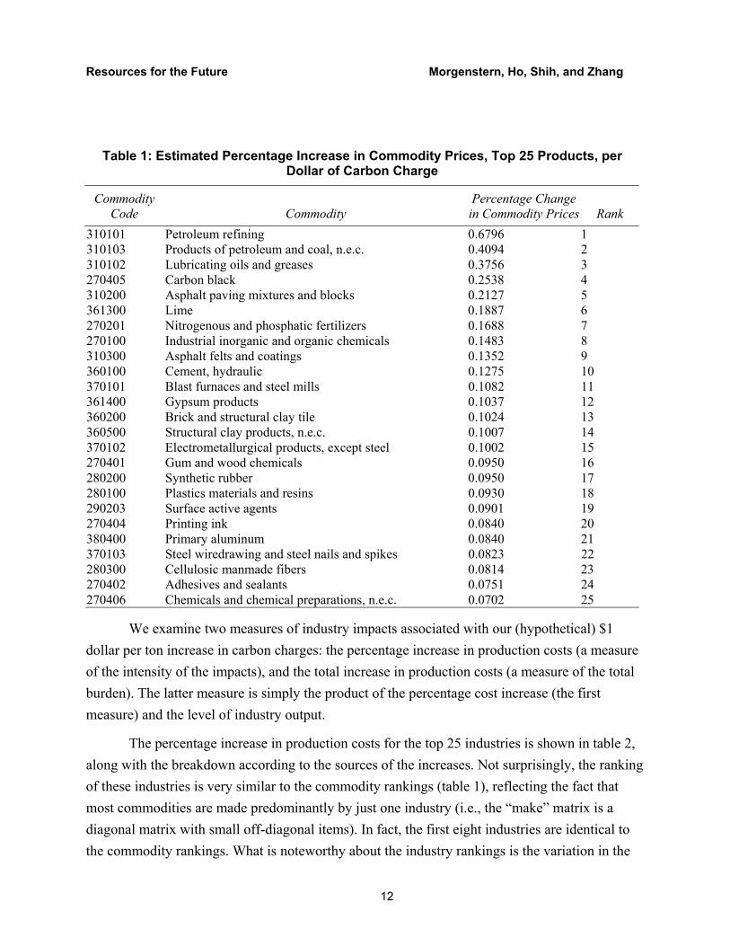
Table 1 displays the percentage increase in commodity prices associated with a one dollar increase in the carbon charge for the most heavily affected commodities. Petroleum refining tops the list with an estimated price increase of 0.68% for each additional dollar of carbon charge. Various other refinery products (lubricating oils and greases, asphalt products, carbon black) occupy ranks 2–5, although the average price increase of these other products is only about half as much as petroleum refining.11 Lime ranks 6, followed by fertilizer and chemical products and

9 In competitive unregulated electricity markets, of course, this assumption will not hold. 10 The most recent benchmark U.S. input-output table is the one for 1992. More recent tables are available but they are based on this 1992 benchmark and do not have detailed fuel use supplementary information. 11 This is the effect of a carbon tax placed on primary fuels—the simplest administrative approach. To the extent that some uses of crude oil (or coal) are not combusted, this is not a perfectly targeted greenhouse gas policy. More refined policies might allow for credits or rebates for nonfuel uses of carbon.


11

by cement. By the time you get down to the 25th commodity (chemicals and other chemical preparations), the price increase is only about one-tenth as much as for petroleum refining. Among the entire list of 361 commodities, prices vary by two orders of magnitude.12 Overall, based on equation 17 and reflecting the number of tons of carbon emitted in 1992, the effect on final users of these higher commodity prices due to the $1 per ton carbon charge is to raise total expenditures by $1.35 billion per year ($1992).

12 The complete estimates, across 361 commodities and industries, are available from the authors.


12

Table 1: Estimated Percentage Increase in Commodity Prices, Top 25 Products, per Dollar of Carbon Charge

Commodity Code Commodity

Percentage Change in Commodity Prices Rank

310101 Petroleum refining 0.6796 1 310103 Products of petroleum and coal, n.e.c. 0.4094 2 310102 Lubricating oils and greases 0.3756 3 270405 Carbon black 0.2538 4 310200 Asphalt paving mixtures and blocks 0.2127 5 361300 Lime 0.1887 6 270201 Nitrogenous and phosphatic fertilizers 0.1688 7 270100 Industrial inorganic and organic chemicals 0.1483 8 310300 Asphalt felts and coatings 0.1352 9 360100 Cement, hydraulic 0.1275 10 370101 Blast furnaces and steel mills 0.1082 11 361400 Gypsum products 0.1037 12 360200 Brick and structural clay tile 0.1024 13 360500 Structural clay products, n.e.c. 0.1007 14 370102 Electrometallurgical products, except steel 0.1002 15 270401 Gum and wood chemicals 0.0950 16 280200 Synthetic rubber 0.0950 17 280100 Plastics materials and resins 0.0930 18 290203 Surface active agents 0.0901 19 270404 Printing ink 0.0840 20 380400 Primary aluminum 0.0840 21 370103 Steel wiredrawing and steel nails and spikes 0.0823 22 280300 Cellulosic manmade fibers 0.0814 23 270402 Adhesives and sealants 0.0751 24 270406 Chemicals and chemical preparations, n.e.c. 0.0702 25

We examine two measures of industry impacts associated with our (hypothetical) $1 dollar per ton increase in carbon charges: the percentage increase in production costs (a measure of the intensity of the impacts), and the total increase in production costs (a measure of the total burden). The latter measure is simply the product of the percentage cost increase (the first measure) and the level of industry output.

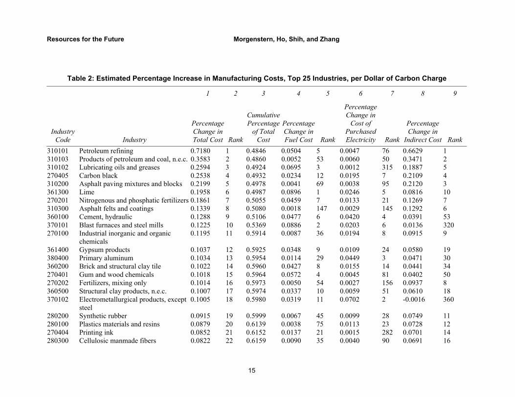
The percentage increase in production costs for the top 25 industries is shown in table 2, along with the breakdown according to the sources of the increases. Not surprisingly, the ranking of these industries is very similar to the commodity rankings (table 1), reflecting the fact that most commodities are made predominantly by just one industry (i.e., the “make” matrix is a diagonal matrix with small off-diagonal items). In fact, the first eight industries are identical to the commodity rankings. What is noteworthy about the industry rankings is the variation in the


13

contribution to the overall cost increases from the different sources—fuel, purchased electricity, and nonenergy intermediate inputs. For example, in the case of petroleum refining, almost all of the increase in manufacturing costs arises from increases in the costs of intermediate inputs (column 8), mostly crude oil. Relatively minor contributions to the overall cost increase arise from direct fuel costs or from purchased electricity (columns 4 and 6). Note that although the petroleum refining industry ranks 1 in overall percentage cost increases (column 2) and in intermediate input costs (column 9), it ranks 7 for direct fuel costs (column 5) and 76 for purchased electricity (column 7).

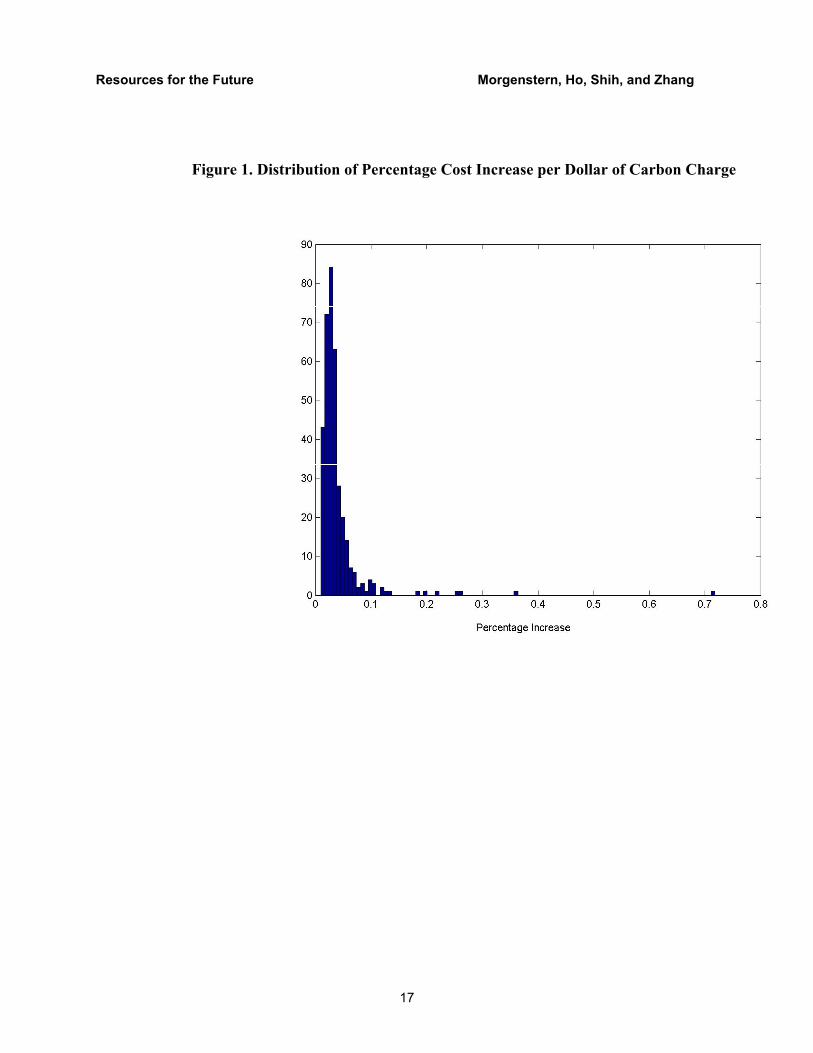
Primary aluminum, ranked 13 in the total percentage increase in costs, displays a somewhat different story. In contrast to petroleum refining, where costs of intermediate inputs dominate, electricity ranks as a more important contributor to cost increases in the primary aluminum industry—almost equal in contribution to intermediate purchases. A still different story emerges in the case of the lime industry, which ranks 6 in overall percentage increases in total costs. Here, the increase in direct fuel costs dominates, and intermediate inputs and purchased electricity make relatively small contributions to total cost increases. As in the case of commodity prices, by the time one gets down to the 25th industry (clay refractories), the price increase is only about one-tenth as much as for the top-ranked petroleum refining. Among the entire list of 361 manufacturing industries, price increases vary by two orders of magnitude. In figure 1 we graph the distribution of cost effects over these 361 sectors. Clearly, a small number of manufacturing industries bear a disproportionate burden of the carbon mitigation policy modeled here.

The residual method of estimating nonenergy intermediate input costs in equation (21) gives rise to seemingly anomalous results for electrometallurgical products (ranked 18; I-O sector 370102; Standard Industrial Classification, SIC, sector 3313) and the iron and steel foundries sector (ranked 129; I-O sector 370200; SIC sector 332). Recall that the total costs estimated from the input-output matrices assume a common purchase price, whereas the direct combustion and electricity costs are calculated from the detailed Census and Electricity Monthly data. To the extent that individual industries have liquid fuel or electricity costs that differ from the national average, the total costs jCOST∆ will misestimate sector j's costs. The extreme case

of this is illustrated by these two sectors, which use a lot of electricity. The same issue arises in the primary aluminum sector (I-O sector 380400; SIC sector 3334).

According to the Census Bureau, the electrometallurgical industry used 3.92 billion kWh in 1992 to produce $1.160 billion worth of output; iron and steel used 72 billion kWh to produce


14

$11.7 billion; the aluminum industry used 60 billion kWh to produce $5.6 billion. The locations of plants in these sectors, however, are very different: aluminum plants tend to be close to relatively inexpensive hydropower. The result is that the carbon content per kWh for electrometallurgical output is 208 tons/million kWh, for iron and steel it is 180 tons/million kWh, but for aluminum it is only 42 tons/million kWh. With these very different values of

,electricty jθ , equation (20) estimates that the electrometallurgical industry bears an increase in

electricity costs equal to 0.07% of output value, iron and steel bear 0.12%, whereas aluminum bears only a 0.045% increase.

However, from the I-O matrices via equation (18), we estimate that the $1/ton carbon charge raises total costs in the electrometallurgical industry by an amount equal to 0.10% of the value of output, in iron and steel merely 0.037%, but in aluminum it is 0.11%. Why the discrepancy between total costs, and the direct combustion and electricity components, for the electrometallurgical and the iron and steel industries? This is explained by the numbers in the use table. For the electrometallurgical industry the I-O table reports electricity input worth $111 million in 1992; for iron and steel, $499 million; but for aluminum, $1,282 million. If we compared these dollar values with the number of kWh used, the price per kWh charged to iron and steel is less than half that charged to aluminum, and a lot less than for electrometallurgical. There is obviously some discrepancy between the I-O data and the electricity data. Further investigation will be necessary to reconcile them. If the data are indeed correct, then it would indicate that the current I-O table of dimension 484×494 is not sufficiently detailed, and further disaggregation of electricity into fossil fuels, hydro, nuclear, and so forth is necessary.


15

Table 2: Estimated Percentage Increase in Manufacturing Costs, Top 25 Industries, per Dollar of Carbon Charge

1 2 3 4 5 6 7 8 9

Industry Code Industry

Percentage Change in Total Cost Rank

Cumulative Percentage

of Total Cost

Percentage Change in Fuel Cost Rank

Percentage Change in

Cost of Purchased Electricity Rank

Percentage Change in

Indirect Cost Rank 310101 Petroleum refining 0.7180 1 0.4846 0.0504 5 0.0047 76 0.6629 1 310103 Products of petroleum and coal, n.e.c. 0.3583 2 0.4860 0.0052 53 0.0060 50 0.3471 2 310102 Lubricating oils and greases 0.2594 3 0.4924 0.0695 3 0.0012 315 0.1887 5 270405 Carbon black 0.2538 4 0.4932 0.0234 12 0.0195 7 0.2109 4 310200 Asphalt paving mixtures and blocks 0.2199 5 0.4978 0.0041 69 0.0038 95 0.2120 3 361300 Lime 0.1958 6 0.4987 0.0896 1 0.0246 5 0.0816 10 270201 Nitrogenous and phosphatic fertilizers 0.1861 7 0.5055 0.0459 7 0.0133 21 0.1269 7 310300 Asphalt felts and coatings 0.1339 8 0.5080 0.0018 147 0.0029 145 0.1292 6 360100 Cement, hydraulic 0.1288 9 0.5106 0.0477 6 0.0420 4 0.0391 53 370101 Blast furnaces and steel mills 0.1225 10 0.5369 0.0886 2 0.0203 6 0.0136 320 270100 Industrial inorganic and organic

chemicals 0.1195 11 0.5914 0.0087 36 0.0194 8 0.0915 9

361400 Gypsum products 0.1037 12 0.5925 0.0348 9 0.0109 24 0.0580 19 380400 Primary aluminum 0.1034 13 0.5954 0.0114 29 0.0449 3 0.0471 30 360200 Brick and structural clay tile 0.1022 14 0.5960 0.0427 8 0.0155 14 0.0441 34 270401 Gum and wood chemicals 0.1018 15 0.5964 0.0572 4 0.0045 81 0.0402 50 270202 Fertilizers, mixing only 0.1014 16 0.5973 0.0050 54 0.0027 156 0.0937 8 360500 Structural clay products, n.e.c. 0.1007 17 0.5974 0.0337 10 0.0059 51 0.0610 18 370102 Electrometallurgical products, except

steel 0.1005 18 0.5980 0.0319 11 0.0702 2 -0.0016 360

280200 Synthetic rubber 0.0915 19 0.5999 0.0067 45 0.0099 28 0.0749 11 280100 Plastics materials and resins 0.0879 20 0.6139 0.0038 75 0.0113 23 0.0728 12 270404 Printing ink 0.0852 21 0.6152 0.0137 21 0.0015 282 0.0701 14 280300 Cellulosic manmade fibers 0.0822 22 0.6159 0.0090 35 0.0040 90 0.0691 16


16

270402 Adhesives and sealants 0.0762 23 0.6180 0.0014 189 0.0022 204 0.0727 13 290203 Surface active agents 0.0759 24 0.6191 0.0031 84 0.0029 143 0.0699 15 360400 Clay refractories 0.0697 25 0.6194 0.0170 18 0.0054 64 0.0473 29


17

Figure 1. Distribution of Percentage Cost Increase per Dollar of Carbon Charge


18

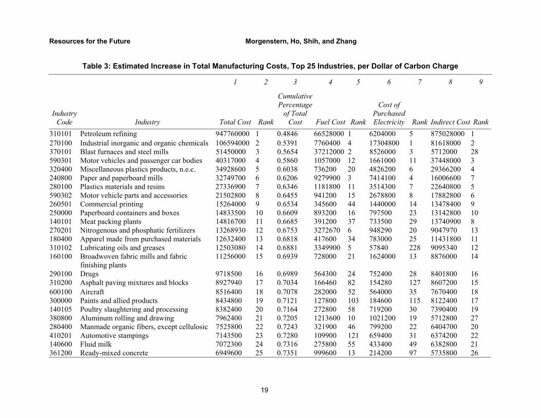
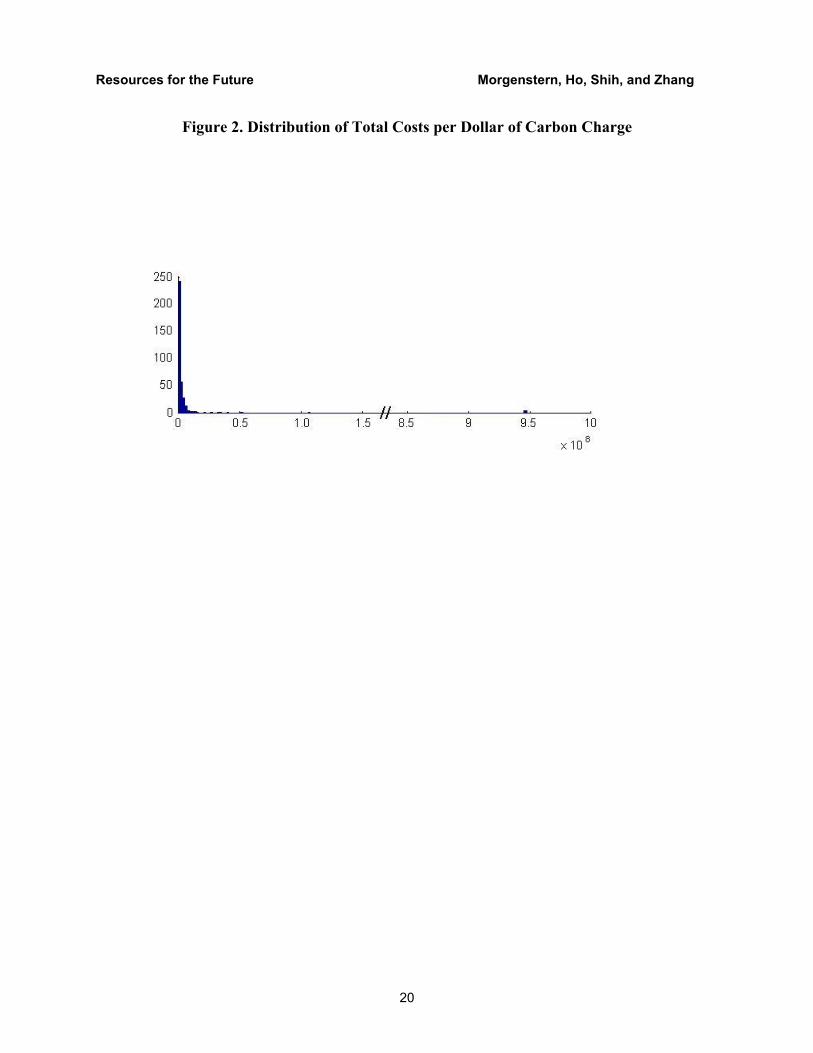
Table 3 displays the total increase in production costs per dollar of increased carbon charge for the top 25 industries. Since we are examining changes in total costs, which reflect both the intensity of the burden and the size of the industry, we would expect a different ordering than observed for the percentage cost increases. Thus, although petroleum refining again tops the list, with total increases in costs of $948 million per dollar increase in carbon charges (equivalent to 48.5% of total costs to the manufacturing sector), the rankings for other industries are quite different. For example, chemicals (inorganic and organic), blast furnaces and steel mills, and motor vehicles and passenger car bodies rank 2, 3, and 4, respectively. Note, however, the steep decline in the increases in total costs as one descends the list. The total costs for inorganic and organic chemicals, ranked 2, are only 11% as much as petroleum refining, ranked 1. Total costs for the drug industry, ranked 16, are only about 1% of the costs for petroleum refining. Overall, a very few manufacturing industries bear the bulk of the sector-wide costs. The top 10 industries, for example, account for about two-thirds of all manufacturing costs, and the top 25 industries account for almost three-fourths of the total. For purposes of comparison, it is noteworthy that the top 25 industries in percentage increase in costs account for a somewhat lower proportion of total costs (column 2 in table 2 versus column 2 in table 3.) Figure 2 displays the distribution of total costs. The extreme skew of the distribution reflects the highly uneven burden among industries.

Also of interest in table 3 are the wide discrepancies in total costs attributable to the different sources of carbon inputs. For example, blast furnaces and steel mills are relatively large purchasers of fuel for direct combustion and of electricity but more modest users of carbon-intensive nonenergy intermediate inputs. In contrast, the motor vehicles and passenger car body industry is a heavy user of nonenergy intermediate inputs (reflecting the many outsourced components used in cars) but a relatively light user of fuels and electricity. Overall, nonenergy intermediate inputs constitute the single largest component of the carbon costs among the 25 industries ranked highest for total manufacturing costs.


19

Table 3: Estimated Increase in Total Manufacturing Costs, Top 25 Industries, per Dollar of Carbon Charge

1 2 3 4 5 6 7 8 9

Industry Code Industry Total Cost Rank

Cumulative Percentage

of Total Cost Fuel Cost Rank

Cost of Purchased Electricity Rank Indirect Cost Rank

310101 Petroleum refining 947760000 1 0.4846 66528000 1 6204000 5 875028000 1 270100 Industrial inorganic and organic chemicals 106594000 2 0.5391 7760400 4 17304800 1 81618000 2 370101 Blast furnaces and steel mills 51450000 3 0.5654 37212000 2 8526000 3 5712000 28 590301 Motor vehicles and passenger car bodies 40317000 4 0.5860 1057000 12 1661000 11 37448000 3 320400 Miscellaneous plastics products, n.e.c. 34928600 5 0.6038 736200 20 4826200 6 29366200 4 240800 Paper and paperboard mills 32749700 6 0.6206 9279900 3 7414100 4 16006600 7 280100 Plastics materials and resins 27336900 7 0.6346 1181800 11 3514300 7 22640800 5 590302 Motor vehicle parts and accessories 21502800 8 0.6455 941200 15 2678800 8 17882800 6 260501 Commercial printing 15264000 9 0.6534 345600 44 1440000 14 13478400 9 250000 Paperboard containers and boxes 14833500 10 0.6609 893200 16 797500 23 13142800 10 140101 Meat packing plants 14816700 11 0.6685 391200 37 733500 29 13740900 8 270201 Nitrogenous and phosphatic fertilizers 13268930 12 0.6753 3272670 6 948290 20 9047970 13 180400 Apparel made from purchased materials 12632400 13 0.6818 417600 34 783000 25 11431800 11 310102 Lubricating oils and greases 12503080 14 0.6881 3349900 5 57840 228 9095340 12 160100 Broadwoven fabric mills and fabric

finishing plants 11256000 15 0.6939 728000 21 1624000 13 8876000 14

290100 Drugs 9718500 16 0.6989 564300 24 752400 28 8401800 16 310200 Asphalt paving mixtures and blocks 8927940 17 0.7034 166460 82 154280 127 8607200 15 600100 Aircraft 8516400 18 0.7078 282000 52 564000 35 7670400 18 300000 Paints and allied products 8434800 19 0.7121 127800 103 184600 115 8122400 17 140105 Poultry slaughtering and processing 8382400 20 0.7164 272800 58 719200 30 7390400 19 380800 Aluminum rolling and drawing 7962400 21 0.7205 1213600 10 1021200 19 5712800 27 280400 Manmade organic fibers, except cellulosic 7525800 22 0.7243 321900 46 799200 22 6404700 20 410201 Automotive stampings 7143500 23 0.7280 109900 121 659400 31 6374200 22 140600 Fluid milk 7072300 24 0.7316 275800 55 433400 49 6382800 21 361200 Ready-mixed concrete 6949600 25 0.7351 999600 13 214200 97 5735800 26


20

Figure 2. Distribution of Total Costs per Dollar of Carbon Charge


21

IV. Policy Comparisons

Despite its intellectual appeal, an economy-wide carbon charge (or upstream emissions trading system) is not the only option for reducing GHG emissions. Various forms of so-called downstream policies have also been discussed. For example, S.556, introduced in the 107th Congress, envisions a tradable permit system imposed on power plants to control carbon dioxide.13 Such an approach would increase the cost of using carbon in electricity generation only. Direct combustion of coal, oil, or gas outside the electric power industry would not be covered.

Table 4 compares the impacts of an economy-wide policy versus an electricity-only policy on manufacturing industries. The per ton charge on carbon inputs is equal for the two policies. However, the former policy affects all carbon inputs, direct and indirect, used in the manufacturing sector, but the latter affects only carbon used in the production of electricity. Manufacturing industries relying heavily on electricity or nonfuel inputs that in turn rely heavily on electricity—for example, the higher cost of aluminum car parts purchased by the auto industry—would be most adversely affected.

The left side of table 4 displays the 10 industries hardest hit by the economy-wide policy and their corresponding ranking (among the 361 manufacturing industries) for the electricity-only policy. Petroleum refining, hardest hit by the economy-wide policy, ranks 145 for the electricity-only policy. Eight of the 10 industries hardest hit by the economy-wide policy rank lower (or the same) for the electricity-only policy—in most cases considerably lower.

The right side of table 4 displays the 10 industries hardest hit by the electricity-only policy along with their corresponding ranking for the economy-wide policy. The hardest hit—aluminum—ranks 13 for the economy-wide policy. All of the top 10 under the electricity-only policy rank lower (or the same) for the economy-wide policy—in many cases substantially lower. The key conclusion of this comparison of alternative policies is clear: manufacturing industries are affected very differently by the economy-wide regulation of carbon versus regulation of the electric power sector only. Many of those industries hardest hit by one policy tend not to be so adversely affected by the other, and vice versa.

13 Regulation of sulfur dioxide, nitrogen oxides, and mercury are also proposed in this so-called Four-Pollutant Bill.


22

Table 4: Comparison of Economy-Wide and Electricity-Only Policies

Ranked by Economy-Wide Policy Ranked by Electricity-Wide Policy

Industry Economy-Wide Carbon Charge Rank

Electricity-Only Carbon Charge Rank Industry

Economy-Wide Carbon Charge Rank

Electricity Only Carbon Charge Rank

Petroleum refining 0.718 1 0.007 145 Primary aluminum 0.103 13 0.064 1 Products of petroleum and coal, n.e.c.

0.358 2 0.006 191 Electrometallurgical products, except steel

0.101 18 0.032 2

Lubricating oils and greases

0.259 3 0.007 154 Cement, hydraulic 0.129 9 0.027 3

Carbon black 0.254 4 0.011 36 Aluminum rolling and drawing

0.054 49 0.021 4

Asphalt paving mixtures and blocks

0.220 5 0.009 76 Primary smelting and refining of copper

0.052 52 0.019 5

Lime 0.196 6 0.017 6 Lime 0.196 6 0.017 6 Nitrogenous and phosphatic fertilizers

0.186 7 0.011 25 Primary nonferrous metals, n.e.c.

0.048 64 0.017 7

Asphalt felts and coatings

0.134 8 0.006 196 Blast furnaces and steel mills

0.123 10 0.016 8

Cement, hydraulic 0.129 9 0.027 3 Metal cans 0.054 48 0.016 9 Blast furnaces and steel mills

0.123 10 0.016 8 Aluminum castings 0.039 95 0.015 10

.


23

V. Comparisons across Model Types and Data Aggregation Levels

The impacts on manufacturing industries of carbon mitigation policies presented in the previous section differ from more commonly available analyses in two principal respects: 1) the focus is on short-term impacts rather than the longer-term effects typically addressed in dynamic, general equilibrium models; and 2) the results are highly disaggregate in nature, based on four-digit industry classification codes rather than the more standard two-digit approach. This section examines the twin questions of how the short- and longer-term results compare and how the two- and four-digit results compare. Answers to the first question can provide insight into whether the industries identified as most heavily impacted in the short term are the same ones predicted to experience long-term burdens as well. Answers to the second question indicate the value of dealing with such a detailed dataset in addressing issues of relative distribution within the manufacturing sector.

A. Short Run versus Long Run

There are two aspects of the short-run versus long-run comparisons: the relative size of the overall price increases estimated in the long-run versus the short-run models, and the relative distribution among the different industries estimated by the different modeling approaches.14 On the first point, the direction of the difference is clear: in the long run, technological innovation and substitutions away from carbon-intensive fuels will tend to drive down costs over time. The only question is by how much. Clearly, the model presented here, which calculates the increase in production costs assuming fixed capital and other inputs, should be seen as an upper-bound estimate of the price changes in individual industries. As noted, the real value of the analysis is its relevance to relative burdens within the manufacturing sector rather than as a measure of absolute costs.

We should discuss here the different uses of the word "cost" in the literature. When economists using the long-run models say that carbon control costs x% of GDP, they mean that the reduction in welfare when consumption patterns change in response to changes in prices is

14 By long-run analyses we mean those that allow substitution among inputs, whether or not the substitution occurs within a static or dynamic framework. Dynamic models allow a richer set of changes, like investment and technology change, but static models that allow substitution would still show a much smaller change than what we refer to as short-run analysis.


24

equal to x% of GDP. One way to think about this is that society is forced by the tax wedges to move to a different point on the production possibilities frontier (PPF), a point that delivers lower utility. This does not mean that the PPF has shrunk or that some workers are idle. In the short run, the welfare costs to society should include adjustment costs as capital and labor are reallocated; that is, the PPF might actually shrink during the transition. This is not what is calculated in this paper. What is calculated is the increase in the bill for intermediate inputs for an industry, assuming the full price changes have been passed through to it. If the industry, in turn, passes on 100% of these costs, then the price of its output rises by the amount tabulated. The welfare costs to the owners and workers of the firm are distinct from these price changes, although they could well be related.15

We shall therefore not be discussing welfare costs but price changes. For the relative price changes among industries, the differences between the long run and the short run are not obvious a priori. Since individual industries exhibit different degrees of factor substitution and technological change, the relative impacts over time may differ across industries. One way to think about this issue is to compare our results with those of a long-run, dynamic model. The most disaggregate model we are aware of is the one developed by Jorgensen and Wilcoxen (1993) and Ho and Jorgensen (1998), which presents estimates at the modified two-digit I-O level for 21 manufacturing industries.

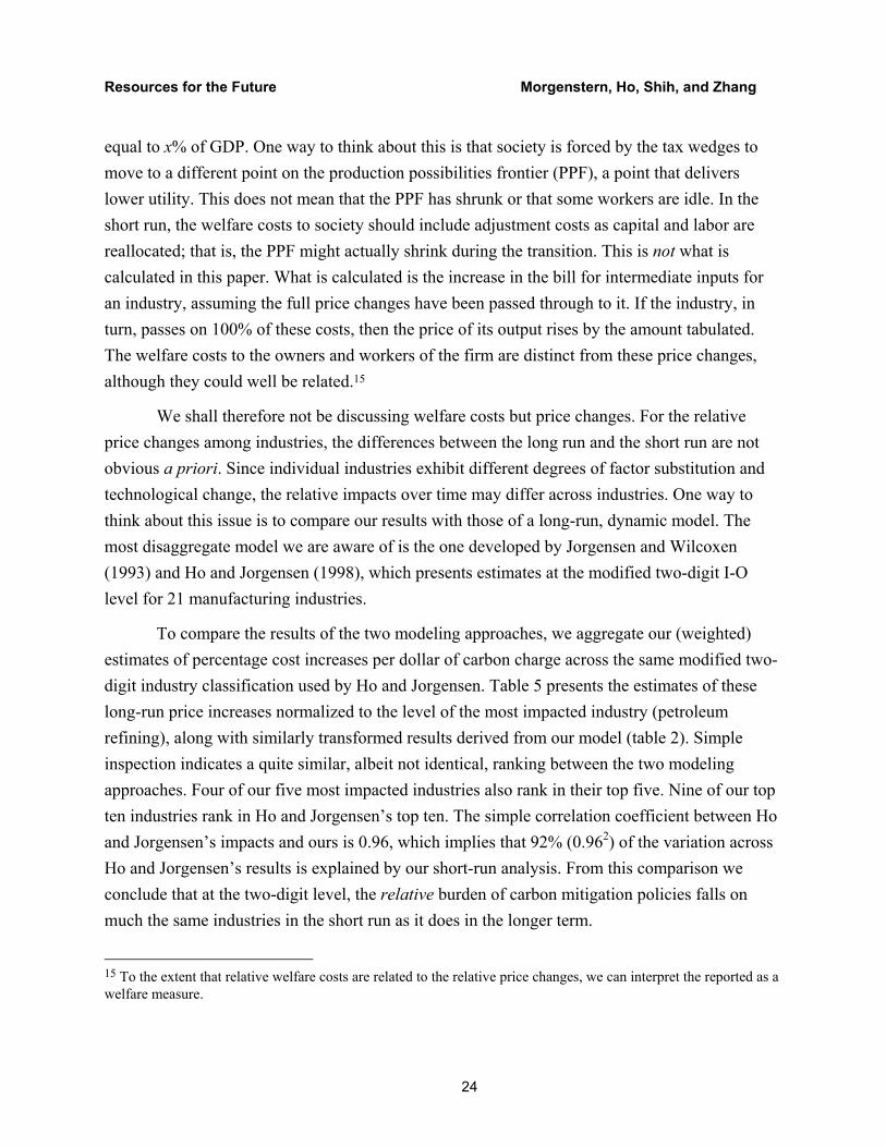
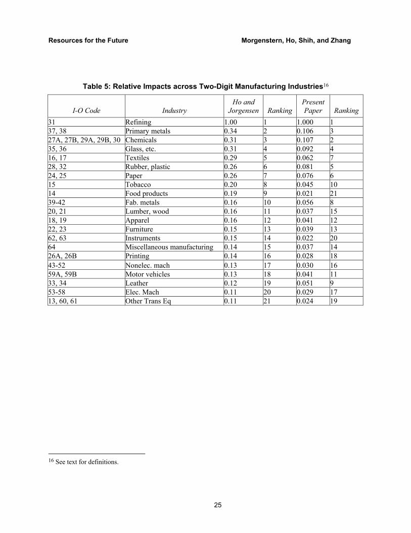
To compare the results of the two modeling approaches, we aggregate our (weighted) estimates of percentage cost increases per dollar of carbon charge across the same modified two-digit industry classification used by Ho and Jorgensen. Table 5 presents the estimates of these long-run price increases normalized to the level of the most impacted industry (petroleum refining), along with similarly transformed results derived from our model (table 2). Simple inspection indicates a quite similar, albeit not identical, ranking between the two modeling approaches. Four of our five most impacted industries also rank in their top five. Nine of our top ten industries rank in Ho and Jorgensen’s top ten. The simple correlation coefficient between Ho and Jorgensen’s impacts and ours is 0.96, which implies that 92% (0.962) of the variation across Ho and Jorgensen’s results is explained by our short-run analysis. From this comparison we conclude that at the two-digit level, the relative burden of carbon mitigation policies falls on much the same industries in the short run as it does in the longer term.

15 To the extent that relative welfare costs are related to the relative price changes, we can interpret the reported as a welfare measure.


25

Table 5: Relative Impacts across Two-Digit Manufacturing Industries16

I-O Code Industry Ho and

Jorgensen Ranking Present Paper Ranking

31 Refining 1.00 1 1.000 1 37, 38 Primary metals 0.34 2 0.106 3 27A, 27B, 29A, 29B, 30 Chemicals 0.31 3 0.107 2 35, 36 Glass, etc. 0.31 4 0.092 4 16, 17 Textiles 0.29 5 0.062 7 28, 32 Rubber, plastic 0.26 6 0.081 5 24, 25 Paper 0.26 7 0.076 6 15 Tobacco 0.20 8 0.045 10 14 Food products 0.19 9 0.021 21 39-42 Fab. metals 0.16 10 0.056 8 20, 21 Lumber, wood 0.16 11 0.037 15 18, 19 Apparel 0.16 12 0.041 12 22, 23 Furniture 0.15 13 0.039 13 62, 63 Instruments 0.15 14 0.022 20 64 Miscellaneous manufacturing 0.14 15 0.037 14 26A, 26B Printing 0.14 16 0.028 18 43-52 Nonelec. mach 0.13 17 0.030 16 59A, 59B Motor vehicles 0.13 18 0.041 11 33, 34 Leather 0.12 19 0.051 9 53-58 Elec. Mach 0.11 20 0.029 17 13, 60, 61 Other Trans Eq 0.11 21 0.024 19

16 See text for definitions.


26

B. The Value of Disaggregating at the Four-Digit Level

Figure 3 displays the distributions of estimated changes in industry costs of four-digit industries within each of 21 two-digit industries (the same industries as in table 4). In each subplot, the star on the horizontal axis represents the weighted mean of the percentage increase in costs for that specific two-digit industry. It is clear that the weighted mean can overstate or understate the true burden. The use of the two-digit classification scheme masks sometimes wide, skewed, or even bimodal distributions of costs. This implies that use of an average value for costs for each of the two-digit industries may not be suitable for understanding the specific nature of the industry-level impacts or for designing appropriate remedies.


27

Figure 3. Comparison of Two- and Four-Digit Classification Schemes


28

VI. Conclusions

As the experience of the failed Btu tax demonstrates, policymakers need to understand who pays for carbon mitigation policies. Detailed information on the relative short-term burdens imposed by carbon mitigation policies is a prerequisite for designing appropriate policy responses. The focus in this paper is on manufacturing industries. Thus, we are looking at the impacts on an important class of energy users rather than on the more traditionally studied industries like fossil fuel producers or electricity generators.

To develop industry-specific estimates on the basis of existing data, certain simplifying assumptions are adopted about both the type of carbon mitigation policies employed and the nature of the behavioral responses in the economy. The principal policy considered is a market-based approach that fixes a uniform cost per ton of carbon via an upstream permit or tax placed on primary fossil fuels (coal, crude oil, natural gas). A downstream policy focused exclusively on the electric power industry is also examined. Regarding the economic response, we assume the per ton costs of the carbon mitigation policy are passed on in the short run in proportion to carbon use. This approach, which freezes capital and other inputs at current levels and assumes that all costs are passed forward, yields upper-bound estimates of total costs. Thus, the results should be viewed as descriptive of relative burdens within the manufacturing sector rather than as a measure of absolute costs. Given these assumptions, the conclusions of this paper can be summarized as follows:

• The variation in estimated end-user price impacts is considerable—about two orders of magnitude—when viewed across the 361 commodities examined. Only a relatively small number of commodities experience the large increases.

• The variation in industry-level cost impacts, measured as the percentage change in costs, is also about two orders of magnitude. Like the commodity price effects, the distribution is highly skewed toward the lower end. Only a few industries experience relatively large burdens.

• There is considerable variability within industries regarding the causes of the estimated cost increases. For some industries, the cost increase is driven by interindustry purchases of nonenergy intermediate inputs. For others, direct fuel costs or purchased electricity is most important.


29

• Total industry cost increases, reflecting the percentage cost increases and industry size, vary by four orders of magnitude across the 361 manufacturing industry categories examined. For the economy-wide carbon policy, a single industry, petroleum, accounts for almost half of the total cost to the manufacturing sector, largely reflecting increased costs for purchased crude oil. The top 10 industries account for almost two-thirds of the total cost to the manufacturing sector.

• With a downstream policy, such as an electricity-only approach, similar cross-industry variation is observed, but a very different set of industries is affected. In fact, many of the industries hardest hit by the economy-wide policy tend not to be so adversely affected by the electricity-only policy, and vice versa.

Overall, the principal conclusion of this research is that within the manufacturing sector (which by definition excludes coal production and electricity generation), only a small number of industries would bear a disproportionate short-term burden of a carbon mitigation policy. Even this statement needs to be qualified, however, since some or all of this burden is likely to be shifted forward by these industries to their customers. In effect, the who pays issue addressed here is more accurately described as who pays initially. The ultimate effect on corporate profits may be negligible (or even positive). As the policy process places greater emphasis on the who pays issue, information on the identity of the affected industries and the magnitude of the disproportionate (initial) burdens borne by a few manufacturing industries can prove invaluable in designing policies to make the distributional impacts more uniform, thereby avoiding the concentration of costs on a few key industries. This knowledge may enhance the political feasibility of future carbon mitigation policies.


30

References

Bureau of Economic Analysis (BEA). 1997. 1992 I-O benchmark working level data.

Burtraw, Dallas, Karen Palmer, Ranjit Bharvikar, and Anthony Paul. 2001. The Effect of Allowance Allocation on the Cost of Carbon Emission Trading. RFF Discussion Paper 01-30. Washington, DC: Resources for the Future.

Energy Information Administration (EIA). 1993. Electric Power Monthly. Washington, DC: Department of Energy.

______. 1994. Manufacturing Consumption of Energy 1991. Washington, DC: Department of Energy.

______. 1997a. Emissions of Greenhouse Gases in the United States 1996. Washington, DC: Department of Energy.

______. 1997b. State Energy Price and Expenditure Report 1997. Available at http://www.eia.doe.gov/emeu/seper/contents.html. Accessed fall 2001.

______. 2000. Annual Energy Outlook 2001. Available at http://www.eia.doe.gov/oiaf/aeo/assumption/tbl2.html. Accessed fall 2001.

Goulder, Lawrence. 2001. Mitigating the Adverse Impacts of CO2 Abatement Policies on Energy Intensive Industries. Paper presented at RFF workshop on the Distributional Impacts of Carbon Mitigation Policies, December 11, 2001, Washington, DC.

Ho, Mun S., and Dale W. Jorgensen. 1998. Stabilization of Carbon Emissions and International Competitiveness of U.S. Industries. In Growth Vol. 2: Energy, the Environment, and Economic Growth, edited by Dale Jorgensen. Cambridge, MA: MIT Press.

Jorgensen, Dale W., and Peter J. Wilcoxen. 1993. Reducing U.S. Carbon Dioxide Emissions: An Assessment of Alternative Instruments. Journal of Policy Modeling 15(5–6): 491–520.

Kolb, Jeffrey. 2001. Personal communication with the authors.

Miller, Ronald E., and Peter D. Blair. 1985. Input-Output Analysis: Foundations and Extensions. Englewood Cliffs, NJ: Prentice-Hall, Inc.

Olson, Mancur. 1965. The Logic of Collective Action. Cambridge, MA: Harvard University Press.


31

U.S. Bureau of the Census. 1994. 1992 Economic Census CD ROM. Washington, DC: U.S. Department of Commerce.

Weyant, John P., and Jennifer N. Hill. 1999. Introduction and Overview. Energy Journal (Kyoto Special Issue): I-xliv.


32

Appendix: Derivation of Direct Combustion and Electricity Factors

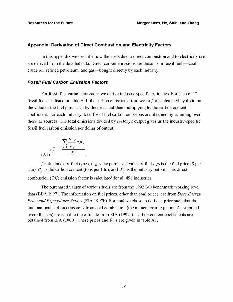
In this appendix we describe how the costs due to direct combustion and to electricity use are derived from the detailed data. Direct carbon emissions are those from fossil fuels—coal, crude oil, refined petroleum, and gas—bought directly by each industry.

Fossil Fuel Carbon Emission Factors

For fossil fuel carbon emissions we derive industry-specific estimates. For each of 12 fossil fuels, as listed in table A-1, the carbon emissions from sector j are calculated by dividing the value of the fuel purchased by the price and then multiplying by the carbon content coefficient. For each industry, total fossil fuel carbon emissions are obtained by summing over these 12 sources. The total emissions divided by sector j's output gives us the industry-specific fossil fuel carbon emission per dollar of output:

(A1)

12

1*fj

ff fDC

jj

pvp

cX

θ=

=∑

.

f is the index of fuel types, pvfj is the purchased value of fuel f, pf is the fuel price ($ per Btu), fθ is the carbon content (tons per Btu), and jX is the industry output. This direct

combustion (DC) emission factor is calculated for all 498 industries.

The purchased values of various fuels are from the 1992 I-O benchmark working level data (BEA 1997). The information on fuel prices, other than coal prices, are from State Energy Price and Expenditure Report (EIA 1997b). For coal we chose to derive a price such that the total national carbon emissions from coal combustion (the numerator of equation A1 summed over all users) are equal to the estimate from EIA (1997a). Carbon content coefficients are obtained from EIA (2000). These prices and fθ 's are given in table A1.


33

Table A1: Price and Carbon Content of Selected Fuels

Fuel Type

Pricea

($/MBtu)

Carbon Contente (MMTCE per

Quadrillion Btu) Bituminous coal and lignite mining

1.91b 25.29

Anthracite mining 1.91b 25.29 Crude petroleum 15.99d 20.22 Natural gas liquid 3.59 16.99 Natural gas 3.89 14.40 Aviation gasoline 8.18 19.14 Motor gasoline 8.96 19.14 Jet fuel 4.52 19.14 Light fuel oil 7.11 19.75 Heavy fuel oil 2.27 21.28 Liquefied petroleum gases 6.19 17.11 Coke and breeze 2.15 25.51f a. Fuel prices are from State Energy Price and Expenditure Report (EIA 1997b) unless noted.

b. Derived by authors, so that national carbon emissions from coal combustion equal that estimated in EIA (1997a), table 5.

c. Crude petroleum is considered only in the refining industry. Crude petroleum purchased by other industries is considered feedstock. Thus, carbon emissions from purchased crude are not calculated for other industries. Crude petroleum can be used for two purposes in the refining industry: as a feedstock or as a fuel. We assume that 10% of crude (on a basis of Btu content) is used as a fuel and 90% as a feedstock (Kolb 2001).

d. The price is in U.S. $/bbl. This is converted to $/Btu using a rate of 6.056 MBtu/bbl obtained from Manufacturing Energy Consumption Survey 1991 (EIA 1994).

e. Carbon content (million metric tons of carbon) are from Annual Energy Outlook 2001 (EIA 2000).

f. Derived using data from Emissions of Greenhouse Gases in the United States 1996 (EIA 1997a).

Electricity Carbon Emission Factors

For carbon emissions from purchased electricity, we derive emission factors from data that are more detailed than those for fossil fuels. The derivation involves the following steps:

1. The carbon emissions per unit of electric energy generated are estimated by state using data from Electric Power Monthly.


34

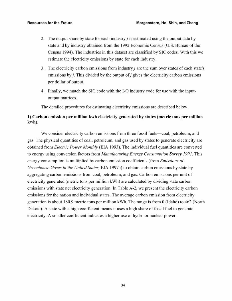
2. The output share by state for each industry j is estimated using the output data by state and by industry obtained from the 1992 Economic Census (U.S. Bureau of the Census 1994). The industries in this dataset are classified by SIC codes. With this we estimate the electricity emissions by state for each industry.

3. The electricity carbon emissions from industry j are the sum over states of each state's emissions by j. This divided by the output of j gives the electricity carbon emissions per dollar of output.

4. Finally, we match the SIC code with the I-O industry code for use with the input-output matrices.

The detailed procedures for estimating electricity emissions are described below.

1) Carbon emission per million kwh electricity generated by states (metric tons per million kwh).

We consider electricity carbon emissions from three fossil fuels—coal, petroleum, and gas. The physical quantities of coal, petroleum, and gas used by states to generate electricity are obtained from Electric Power Monthly (EIA 1993). The individual fuel quantities are converted to energy using conversion factors from Manufacturing Energy Consumption Survey 1991. This energy consumption is multiplied by carbon emission coefficients (from Emissions of Greenhouse Gases in the United States, EIA 1997a) to obtain carbon emissions by state by aggregating carbon emissions from coal, petroleum, and gas. Carbon emissions per unit of electricity generated (metric tons per million kWh) are calculated by dividing state carbon emissions with state net electricity generation. In Table A-2, we present the electricity carbon emissions for the nation and individual states. The average carbon emission from electricity generation is about 180.9 metric tons per million kWh. The range is from 0 (Idaho) to 462 (North Dakota). A state with a high coefficient means it uses a high share of fossil fuel to generate electricity. A smaller coefficient indicates a higher use of hydro or nuclear power.


35

Table A-2. Electricity Carbon Emissions by State

State

Total Electricity Carbon Emissions (1000 metric tons)

Net Electricity Generation

(Million Kwh)

Emission coeff. (Metric Tons per

Million Kwh) Alabama 10857.6 68374.0 158.8 Alaska 492.1 2980.0 165.1 Arizona 7629.8 52722.0 144.7 Arkansas 5419.2 27541.0 196.8 California 6233.6 89701.0 69.5 Colorado 6879.0 23983.0 286.8 Connecticut 1206.7 19308.0 62.5 Delaware 1103.4 4941.0 223.3 District of Columbia 29.9 74.0 403.6 Florida 17847.4 103809.0 171.9 Georgia 10379.8 68908.0 150.6 Hawaii 1161.4 5301.0 219.1 Idaho 0.0 4993.0 0.0 Illinois 11308.0 93424.0 121.0 Indiana 19893.9 71633.0 277.7 Iowa 6741.0 22219.0 303.4 Kansas 6223.3 23606.0 263.6 Kentucky 13500.7 57209.0 236.0 Louisiana 8793.1 43072.0 204.1 Maine 239.3 6021.0 39.7 Maryland 4554.5 29109.0 156.5 Massachusetts 4174.0 25254.0 165.3 Michigan 12424.0 62171.0 199.8 Minnesota 6629.7 29038.0 228.3 Mississippi 2348.9 16187.0 145.1 Missouri 10161.1 41586.0 244.3 Montana 4484.3 18521.0 242.1 Nebraska 3482.1 16510.0 210.9 Nevada 3804.0 16153.0 235.5 New Hampshire 727.3 10853.0 67.0 New Jersey 1550.5 22562.0 68.7 New Mexico 6458.8 20369.0 317.1 New York 9873.3 84002.0 117.5 North Carolina 9306.1 63030.0 147.6 North Dakota 9744.3 21060.0 462.7 Ohio 21933.0 102417.0 214.2 Oklahoma 8806.1 35114.0 250.8 Oregon 979.6 31099.0 31.5 Pennsylvania 18139.9 127446.0 142.3 Rhode Island 26.2 101.0 259.3 South Carolina 4102.6 53597.0 76.5 South Dakota 971.5 4879.0 199.1 Tennessee 9151.4 57253.0 159.8 Texas 49010.9 185738.0 263.9 Utah 5902.6 24461.0 241.3 Vermont 10.6 3365.0 3.1 Virginia 4255.3 37051.0 114.8 Washington 2637.2 63174.0 41.7 West Virginia 11867.8 53339.0 222.5 Wisconsin 7700.7 34386.0 223.9 Wyoming 10580.0 30898.0 342.4 U.S. 381737.6 2110542.0 180.9


36

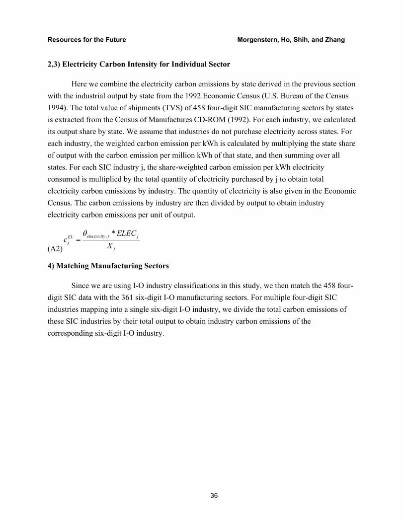
2,3) Electricity Carbon Intensity for Individual Sector

Here we combine the electricity carbon emissions by state derived in the previous section with the industrial output by state from the 1992 Economic Census (U.S. Bureau of the Census 1994). The total value of shipments (TVS) of 458 four-digit SIC manufacturing sectors by states is extracted from the Census of Manufactures CD-ROM (1992). For each industry, we calculated its output share by state. We assume that industries do not purchase electricity across states. For each industry, the weighted carbon emission per kWh is calculated by multiplying the state share of output with the carbon emission per million kWh of that state, and then summing over all states. For each SIC industry j, the share-weighted carbon emission per kWh electricity consumed is multiplied by the total quantity of electricity purchased by j to obtain total electricity carbon emissions by industry. The quantity of electricity is also given in the Economic Census. The carbon emissions by industry are then divided by output to obtain industry electricity carbon emissions per unit of output.

(A2)

, *electricity j jELj

j

ELECc

Xθ

=

4) Matching Manufacturing Sectors

Since we are using I-O industry classifications in this study, we then match the 458 four-digit SIC data with the 361 six-digit I-O manufacturing sectors. For multiple four-digit SIC industries mapping into a single six-digit I-O industry, we divide the total carbon emissions of these SIC industries by their total output to obtain industry carbon emissions of the corresponding six-digit I-O industry.

the near-term impacts of carbon mitigation policies on ... · pdf filemitigation policies on...

Documents