The Natural Number of Forward Markets for Electricity

9th Annual POWER Conference on Electricity Industry Restructuring

March 19, 2004

Hiroaki Suenaga and Jeffrey WilliamsDepartment of Agricultural and Resource Economics

University of California, Davis

suenaga@primal.ucdavis.edu, williams@primal.ucdavis.edu

2

Common observations about electricity:

(1) Extremely volatile prices in spot wholesale markets• short-run capacity constraints

• retail prices inflexible

• pronounced seasonality in demand

• short-run weather shocks

• electricity not storable

(2) Underdeveloped forward wholesale markets• most efforts by exchanges have failed

• California PX restrained to one-day-ahead

• generally, private bilateral trades

3

Our propositions:

• Because of electricity’s very properties, long-dated forward markets for electricity are essentially redundant.

• The NYMEX natural gas futures market duplicates an electricity futures market.

4

How to demonstrate that some price is redundantif it cannot be observed?

• An idealized world for trading electricity• full profile of forward prices

• forward prices are best possible forecasts by construction

• companion forward prices for a fuel

• An analogy with corn• considerable price variation recently

• well developed futures market

5

Progressions of Prices of Corn Futures Contracts

9.88 cents

7.63

3.60

150

200

250

300

350

400

450

5001 2 3 4 5 6 7 8 9 10 11 12 13 14 15 16 17 18 19 20 21

Business days (5/15 - 6/13)

Cents per

bushel

July '96 Dec '96 Dec '97Correlation

of price changes

.45

.81

.40

Std. Dev.of pricechanges

5

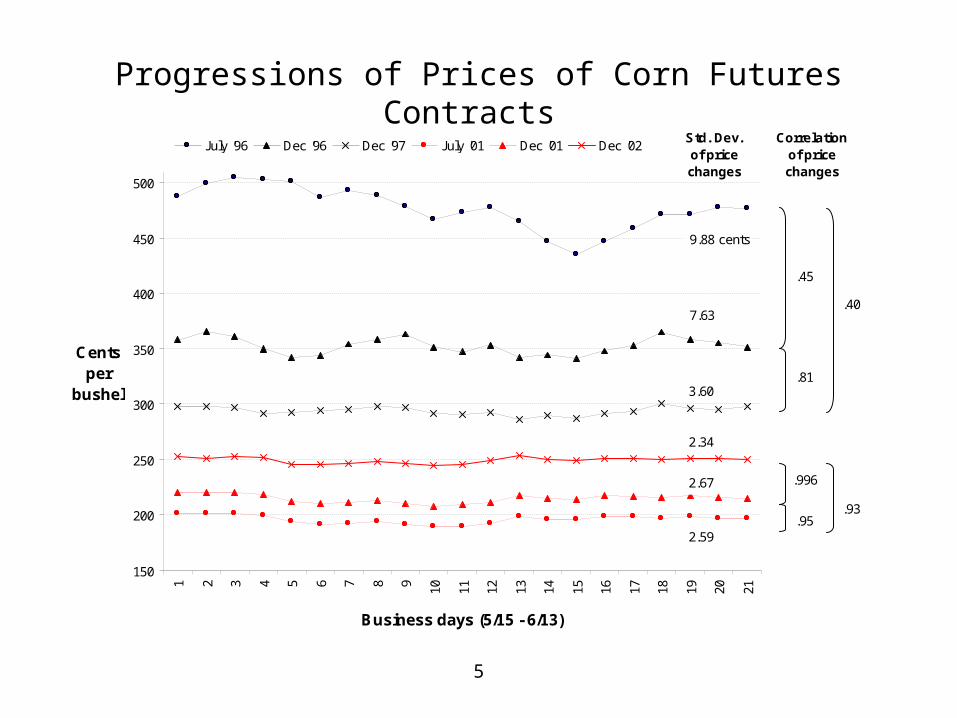
Progressions of Prices of Corn Futures Contracts

9.88 cents

7.63

3.60

2.59

2.67

2.34

150

200

250

300

350

400

450

5001 2 3 4 5 6 7 8 9 10 11 12 13 14 15 16 17 18 19 20 21

Business days (5/15 - 6/13)

Cents per

bushel

July '96 Dec '96 Dec '97 July '01 Dec '01 Dec '02Correlation

of price changes

.45

.81

.40

.996

.95.93

Std. Dev.of pricechanges

6

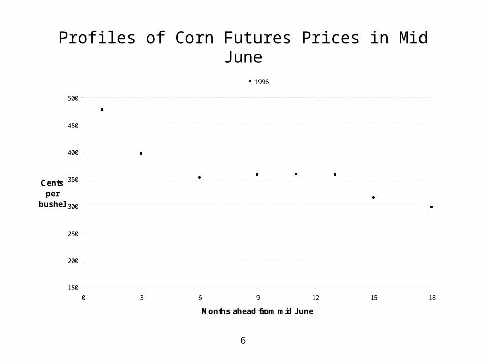
Profiles of Corn Futures Prices in Mid June

150

200

250

300

350

400

450

500

0 3 6 9 12 15 18

Months ahead from mid June

Cents per

bushel

1996

6

Profiles of Corn Futures Prices in Mid June

150

200

250

300

350

400

450

500

0 3 6 9 12 15 18

Months ahead from mid June

Cents per

bushel

1996 2001

6

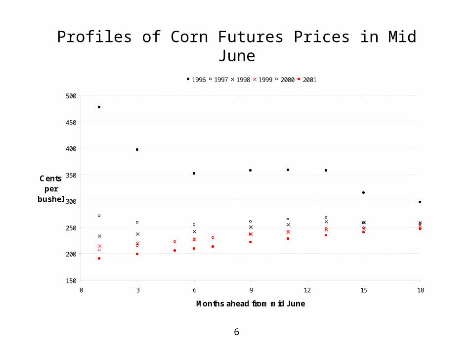
Profiles of Corn Futures Prices in Mid June

150

200

250

300

350

400

450

500

0 3 6 9 12 15 18

Months ahead from mid June

Cents per

bushel

1996 1997 1998 1999 2000 2001

7

Idealized Market Model (Spot Market)

• Generating and retailing firms trade wholesale electricity for a full constellation of delivery hours and days, far into the future.

• All firms are competitive and risk-neutral.

• Aggregate supply:

PSt = b wt Qc-1(1 + MC e1,t) e1,t = MC e1,t -1 + u1,t

where wt = price of primary input (fuel)

b, c, MC, MC = parameters

u1,t ~ iid N(0,1)

• Retail demand is exogenously determined (QAt).

Equilibrium spot price in any hour: Pt = b wt QAtc-1(1 + MC e1,t)

8

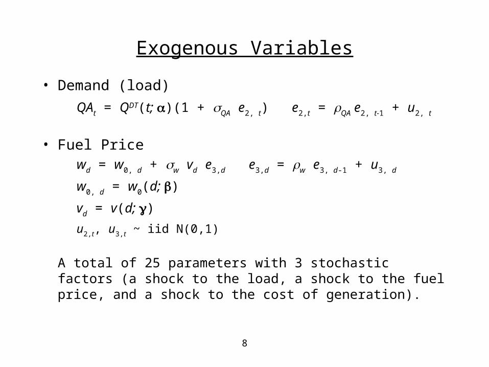
Exogenous Variables

• Demand (load)

QAt = QDT(t; )(1 + QA e2, t) e2,t = QA e2, t-1 + u2, t

• Fuel Pricewd = w0, d + w vd e3,d e3,d = w e3, d-1 + u3, d

w0, d = w0(d; )

vd = v(d; )

u2,t, u3,t ~ iid N(0,1)

A total of 25 parameters with 3 stochastic factors (a shock to the load, a shock to the fuel price, and a shock to the cost of generation).

9

Seasonal and Diurnal Variations in Deterministic Load: QDTt

131

61

9112115

118121

124127

130133

1361

15

913

1721

0

20

40

60

80

100

120

140

160

Load

Day count

Hour of day

10

Seasonal cycles in fuel price and price variance

w 0(d ; )

v (d ; )

0.0

0.5

1.0

1.5

2.0

2.5

3.0

3.5

4.0

1 31 61 91 121

151

181

211

241

271

301

331

361

Day count (d ) from January 1

11

Simulated data - 3 price relationships

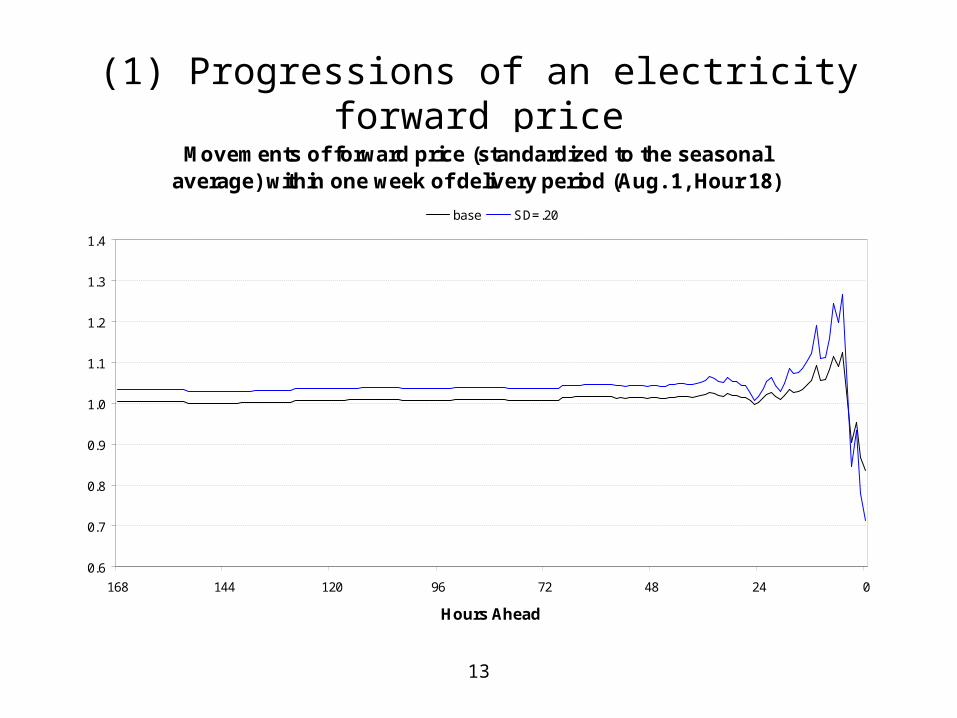
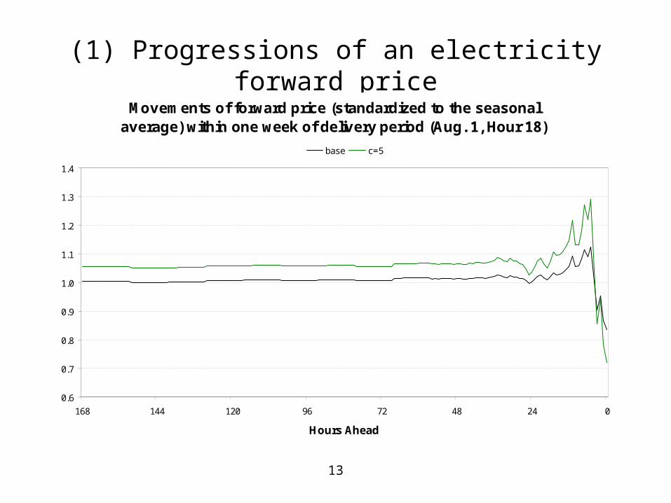
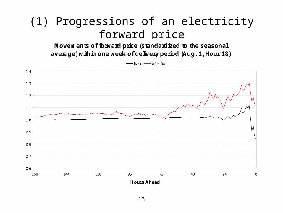
(1) Examine forward profiles – For each delivery hour t, generate as many forward prices, Ft,t-k, as the number of k. Each is the best, unbiased forecast by construction (Ft,t-k = Et-k[Pt]).

If the profiles consistently attenuate to a stable price, forward prices beyond that time ahead are redundant.

(2) Examine spreads

If the spread between the forward prices of two distinct delivery hours is stable, one price can be deduced from the other.

(3) Compare the forecasting ability of the forward price of primary input (wt,t-k) with that of the forward electricity price (Ft,t-k).

If the price movements of the two commodities are highly correlated, one forward price can be deduced from the other.

12

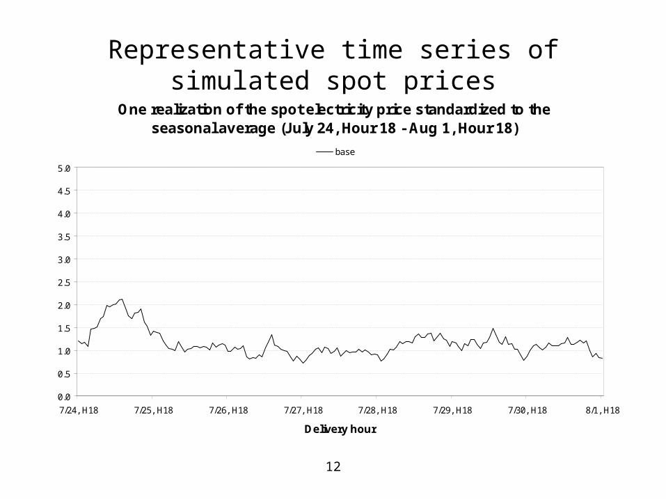
Representative time series of simulated spot prices

One realization of the spot electricity price standardized to the seasonal average (July 24, Hour 18 - Aug 1, Hour 18)

0.0

0.5

1.0

1.5

2.0

2.5

3.0

3.5

4.0

4.5

5.0

7/24, H18 7/25, H18 7/26, H18 7/27, H18 7/28, H18 7/29, H18 7/30, H18 8/1, H18

Delivery hour

base

12

Representative time series of simulated spot prices

One realization of the spot electricity price standardized to the seasonal average (July 24, Hour 18 - Aug 1, Hour 18)

0.0

0.5

1.0

1.5

2.0

2.5

3.0

3.5

4.0

4.5

5.0

7/24, H18 7/25, H18 7/26, H18 7/27, H18 7/28, H18 7/29, H18 7/30, H18 8/1, H18

Delivery hour

base SD=.20

12

Representative time series of simulated spot prices

One realization of the spot electricity price standardized to the seasonal average (July 24, Hour 18 - Aug 1, Hour 18)

0.0

0.5

1.0

1.5

2.0

2.5

3.0

3.5

4.0

4.5

5.0

7/24, H18 7/25, H18 7/26, H18 7/27, H18 7/28, H18 7/29, H18 7/30, H18 8/1, H18

Delivery hour

base c=5

12

Representative time series of simulated spot prices

One realization of the spot electricity price standardized to the seasonal average (July 24, Hour 18 - Aug 1, Hour 18)

0.0

0.5

1.0

1.5

2.0

2.5

3.0

3.5

4.0

4.5

5.0

7/24, H18 7/25, H18 7/26, H18 7/27, H18 7/28, H18 7/29, H18 7/30, H18 8/1, H18

Delivery hour

base AR=.98

13

(1) Progressions of an electricity forward price

Movements of forward price (standardized to the seasonal average) within one week of delivery period (Aug. 1, Hour 18)

0.6

0.7

0.8

0.9

1.0

1.1

1.2

1.3

1.4

168 144 120 96 72 48 24 0

Hours Ahead

base

13

(1) Progressions of an electricity forward price

Movements of forward price (standardized to the seasonal average) within one week of delivery period (Aug. 1, Hour 18)

0.6

0.7

0.8

0.9

1.0

1.1

1.2

1.3

1.4

168 144 120 96 72 48 24 0

Hours Ahead

base SD=.20

13

(1) Progressions of an electricity forward price

Movements of forward price (standardized to the seasonal average) within one week of delivery period (Aug. 1, Hour 18)

0.6

0.7

0.8

0.9

1.0

1.1

1.2

1.3

1.4

168 144 120 96 72 48 24 0

Hours Ahead

base c=5

13

(1) Progressions of an electricity forward price

Movements of forward price (standardized to the seasonal average) within one week of delivery period (Aug. 1, Hour 18)

0.6

0.7

0.8

0.9

1.0

1.1

1.2

1.3

1.4

168 144 120 96 72 48 24 0

Hours Ahead

base AR=.98

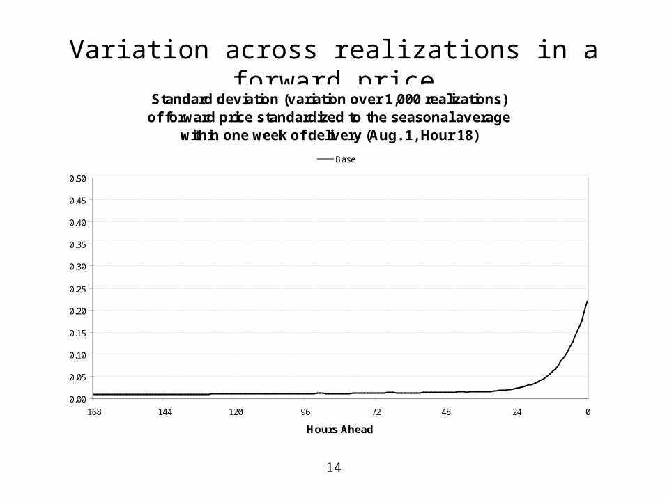
14

Variation across realizations in a forward priceStandard deviation (variation over 1,000 realizations)

of forward price standardized to the seasonal average within one week of delivery (Aug. 1, Hour 18)

0.00

0.05

0.10

0.15

0.20

0.25

0.30

0.35

0.40

0.45

0.50

168 144 120 96 72 48 24 0

Hours Ahead

Base

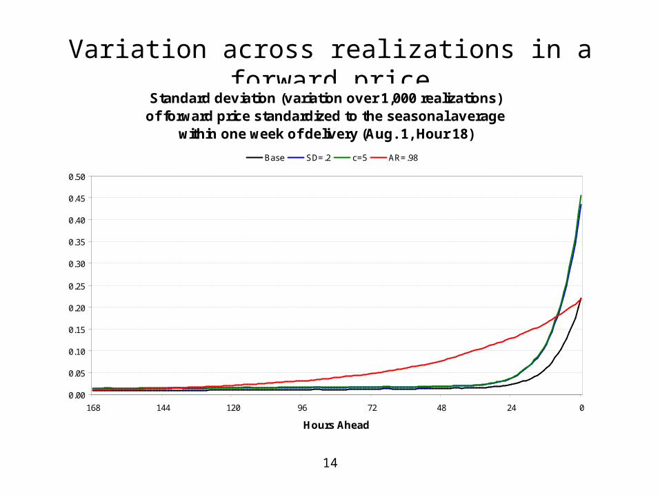
14

Variation across realizations in a forward priceStandard deviation (variation over 1,000 realizations)

of forward price standardized to the seasonal average within one week of delivery (Aug. 1, Hour 18)

0.00

0.05

0.10

0.15

0.20

0.25

0.30

0.35

0.40

0.45

0.50

168 144 120 96 72 48 24 0

Hours Ahead

Base SD=.2 c=5 AR=.98

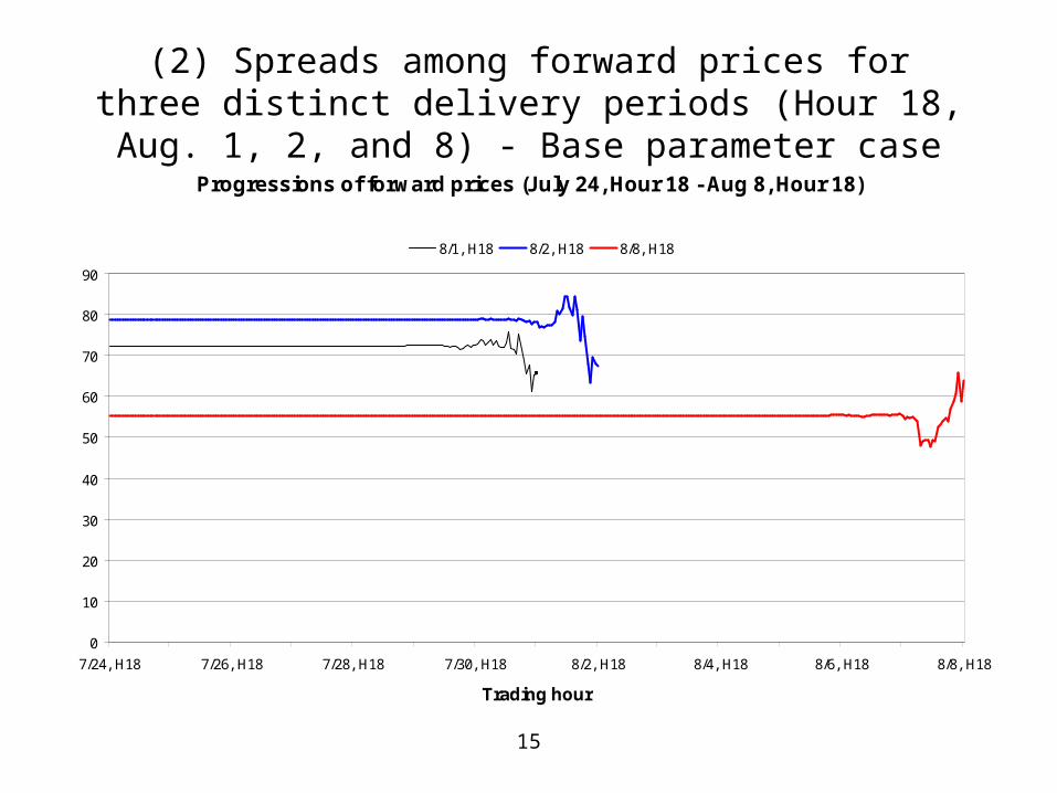
15

(2) Spreads among forward prices for three distinct delivery periods (Hour 18, Aug. 1, 2, and 8) - Base parameter case

Progressions of forward prices (July 24, Hour 18 - Aug 8, Hour 18)

0

10

20

30

40

50

60

70

80

90

7/24, H18 7/26, H18 7/28, H18 7/30, H18 8/2, H18 8/4, H18 8/6, H18 8/8, H18

Trading hour

8/1, H18 8/2, H18 8/8, H18

16

(3) Forecasting ability

• Regression Models

(1) ln Pt = a0 + b0 ln Ft,t-k + e0,t

(2) ln Pt = a2 + b2 ln wt,t-k + c2 ln QFt,t-k + e2,t

Load forecast, QFt,t-k, in (2) allows the market heat rate to be non-constant and vary by season.

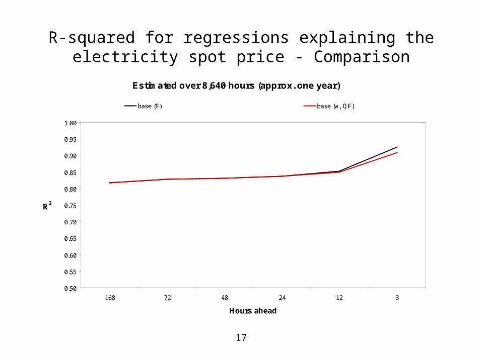
• If the R2 for (2) is close to the R2 for (1), the forward price of fuel predicts the spot electricity price as accurately as the electricity forward.

If so, the benefit from a separate forward market for electricity would be small.

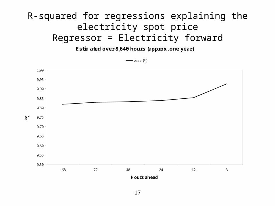
17

R-squared for regressions explaining the electricity spot priceRegressor = Electricity forward

Estimated over 8,640 hours (approx. one year)

0.50

0.55

0.60

0.65

0.70

0.75

0.80

0.85

0.90

0.95

1.00

312244872168

Hours ahead

R2

base (F)

17

R-squared for regressions explaining the electricity spot price - Comparison

Estimated over 8,640 hours (approx. one year)

0.50

0.55

0.60

0.65

0.70

0.75

0.80

0.85

0.90

0.95

1.00

312244872168

Hours ahead

R2

base (F) base (w, QF)

17

R-squared for regressions explaining the electricity spot price - Sensitivity

Estimated over 8,640 hours (approx. one year)

0.50

0.55

0.60

0.65

0.70

0.75

0.80

0.85

0.90

0.95

1.00

312244872168

Hours ahead

R2

base (F) high SD for supply (F) high AR for supply (F)base (w, QF) high SD for supply (w, QF) high AR for supply (w, QF)

18

One-Month-Ahead Forecasting Ability of Corn Futures Contracts (1996-2001)

0

100

200

300

400

500

600

0 100 200 300 400 500 600

July Futures as of Mid June

July Futures at Expiration in Mid July(Cents per

bushel)

R2 = 0.97

19

Six-Month-Ahead Forecasting Ability of Corn Futures Contracts (1996-2001)

0

50

100

150

200

250

300

350

400

0 50 100 150 200 250 300 350 400

December Futures as of Mid June

December Futures at Expiration in Mid Dec(Cents per

bushel)

R2 = 0.52

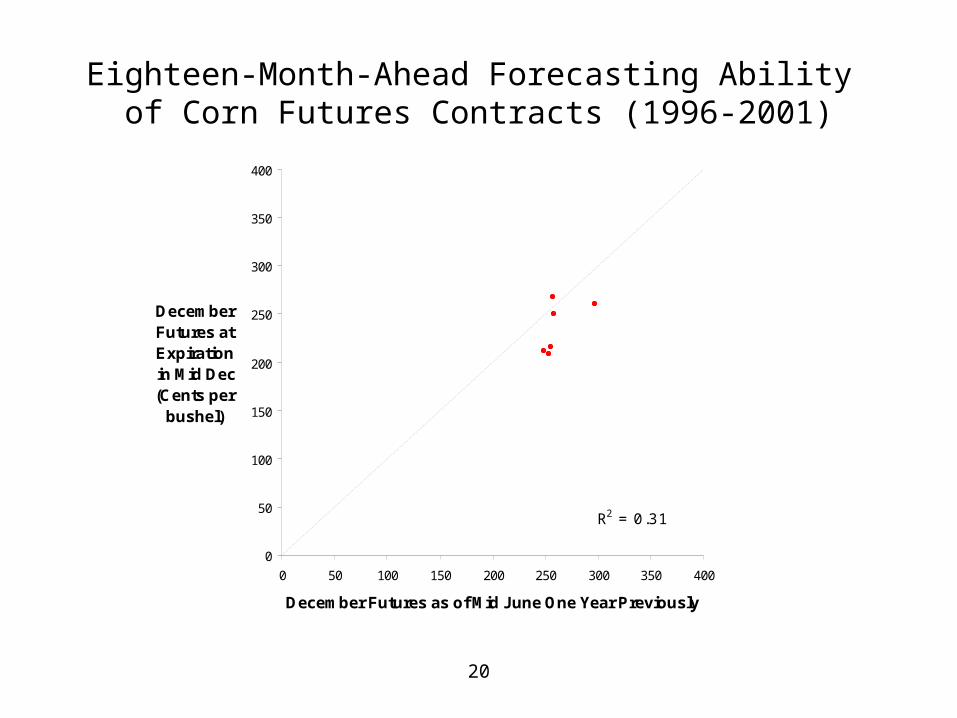
20

Eighteen-Month-Ahead Forecasting Ability of Corn Futures Contracts (1996-2001)

0

100

200

300

400

500

600

0 100 200 300 400 500 600

July Futures as of Mid June

July Futures at Expiration

in Mid July

0

50

100

150

200

250

300

350

400

0 50 100 150 200 250 300 350 400

December Futures as of Mid June One Year Previously

December Futures at Expiration in Mid Dec(Cents per

bushel)

R2 = 0.31

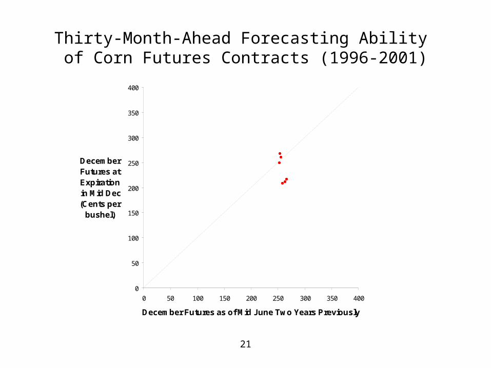
21

Thirty-Month-Ahead Forecasting Ability of Corn Futures Contracts (1996-2001)

0

50

100

150

200

250

300

350

400

0 50 100 150 200 250 300 350 400

Dec Futures as of Mid June

December Futures at Expiration

in Mid Dec

0

50

100

150

200

250

300

350

400

0 50 100 150 200 250 300 350 400

December Futures as of Mid June Two Years Previously

December Futures at Expiration in Mid Dec(Cents per

bushel)

22

Conclusions

• Forecasting ability of electricity forward prices inevitably low.

• Local electricity forward price profiles well represented by:• Local spot markets plus forwards perhaps as far as a week

ahead.

• Regional month-ahead energy forward market, such as natural gas.

• National benchmark long-dated energy forward market, such as the NYMEX natural gas.

• Complex varieties of contracting likely• Local long-dated forward “basis” agreements.