Restricted

The movie plays on:A lens for viewing the global economy

Claudio Borio*Bank for International Settlements

FT Debt Capital Markets Outlook London, 10 February 2016

* Head of the Monetary and Economic Department

2

Theme and takeaways

Objective: to offer a lens to answer the question: Why almost a decade since the Great Financial Crisis (GFC) does the global

economy seem unable to return to sustainable and balanced growth? Three takeaways

Failure to fully come to grips with financial booms and busts- Inability to constrain build-up of financial imbalances (FIs) - Progressive loss of policy room for manoeuvre

Prevailing analytical lens is not fully adequate- Need stronger focus on financial, medium-term and global factors

The road ahead is quite narrow- Economy could rebalance smoothly- But there are risks of further serious financial distress- Policy is key

• Need to abandon debt-fuelled growth model

3

Structure of remarks

Review symptoms of unsustainable and unbalanced global expansion Highlight three of them

Explain the main features of the proposed lens Highlight six of them

Provide the corresponding narrative and identify risks ahead Explain how a faulty lens may have contributed to current predicament

4

I - The symptoms of unbalanced and unsustainable expansion

Symptoms of the malaise: the “ugly three” Debt too high Productivity growth too low Policy room for manoeuvre too limited

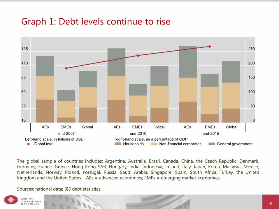
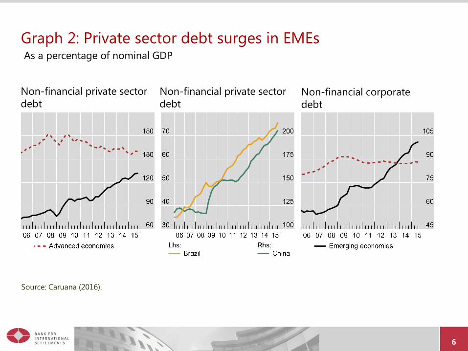
S1: Globally, debt in relation to GDP has not adjusted post-crisis (G 1) Crisis-hit countries: some decline in private sector, increase in public sector Non-crisis-hit countries: increase in private sector (esp EMEs; G 2, 3)), mixed in public sector

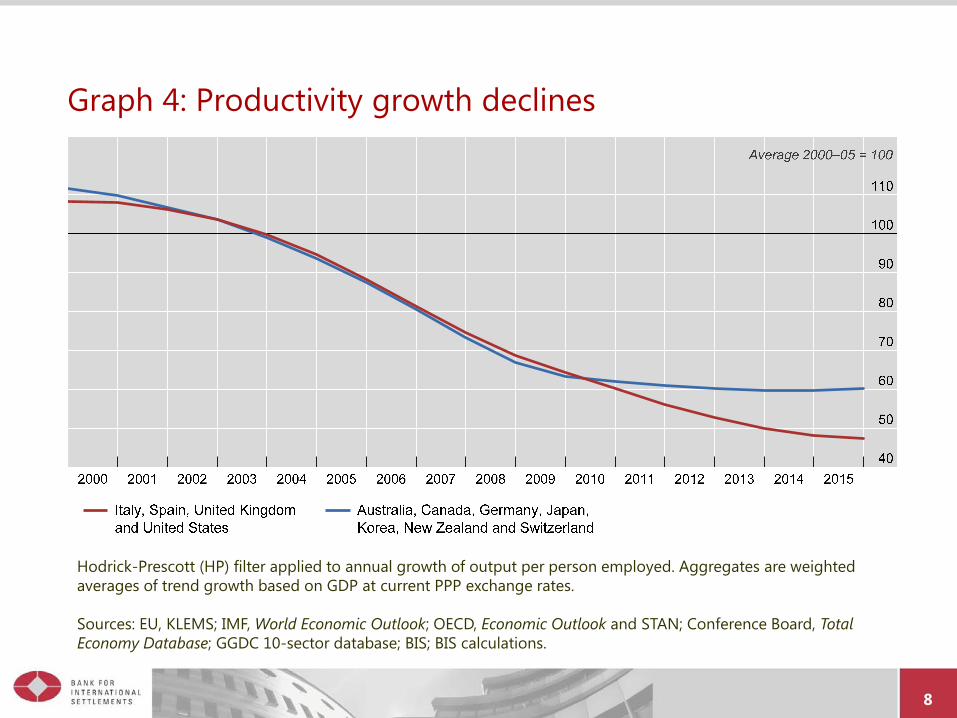
- Several have been exhibiting signs of build-up of FIs S2: Decline in productivity growth (G 4)

Started well before the crisis, intensified thereafter S3: Progressive loss in the policy room for manoeuvre

Fiscal (debt levels) Monetary (policy rates & ballooning balance sheets)

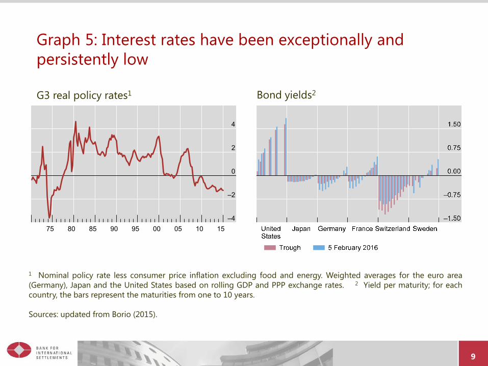
- Persistent ultra-low interest rates, regardless of benchmarks (G 5)- Both policy rates and long-term rates

• New peak: over $6.5 trillion worth of sovereign paper trading at negative yields

5

Graph 1: Debt levels continue to rise

The global sample of countries includes: Argentina, Australia, Brazil, Canada, China, the Czech Republic, Denmark,Germany, France, Greece, Hong Kong SAR, Hungary, India, Indonesia, Ireland, Italy, Japan, Korea, Malaysia, Mexico,Netherlands, Norway, Poland, Portugal, Russia, Saudi Arabia, Singapore, Spain, South Africa, Turkey, the UnitedKingdom and the United States. AEs = advanced economies; EMEs = emerging market economies.

Sources: national data; BIS debt statistics.

10

35

60

85

110

135

0

50

100

150

200

250

AEs EMEs Globalend-2007

AEs EMEs Globalend-2010

AEs EMEs Globalend-2015

Global totalLeft-hand scale, in trillions of USD:

HouseholdsRight-hand scale, as a percentage of GDP:

Non-financial corporates General government

6

Graph 2: Private sector debt surges in EMEsAs a percentage of nominal GDP

Non-financial private sector debt

Non-financial private sector debt

Non-financial corporate debt

Source: Caruana (2016).

7

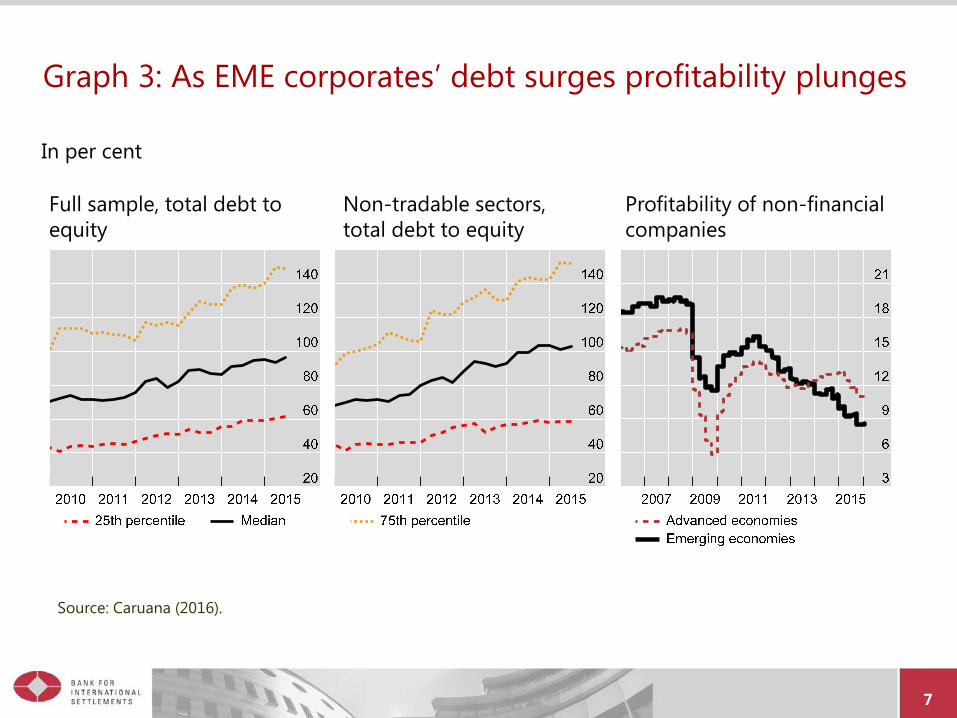
Graph 3: As EME corporates’ debt surges profitability plunges

In per cent

Full sample, total debt to equity

Non-tradable sectors, total debt to equity

Profitability of non-financial companies

Source: Caruana (2016).

8

Graph 4: Productivity growth declines

Hodrick-Prescott (HP) filter applied to annual growth of output per person employed. Aggregates are weighted averages of trend growth based on GDP at current PPP exchange rates.

Sources: EU, KLEMS; IMF, World Economic Outlook; OECD, Economic Outlook and STAN; Conference Board, Total Economy Database; GGDC 10-sector database; BIS; BIS calculations.

9

Graph 5: Interest rates have been exceptionally and persistently low

G3 real policy rates1 Bond yields2

1 Nominal policy rate less consumer price inflation excluding food and energy. Weighted averages for the euro area(Germany), Japan and the United States based on rolling GDP and PPP exchange rates. 2 Yield per maturity; for eachcountry, the bars represent the maturities from one to 10 years.

Sources: updated from Borio (2015).

–4

–2

0

2

4

75 80 85 90 95 00 05 10 15

10

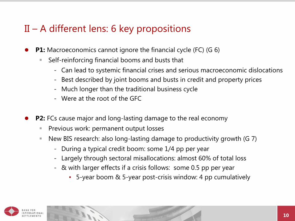
II – A different lens: 6 key propositions

P1: Macroeconomics cannot ignore the financial cycle (FC) (G 6) Self-reinforcing financial booms and busts that

- Can lead to systemic financial crises and serious macroeconomic dislocations- Best described by joint booms and busts in credit and property prices- Much longer than the traditional business cycle- Were at the root of the GFC

P2: FCs cause major and long-lasting damage to the real economy Previous work: permanent output losses New BIS research: also long-lasting damage to productivity growth (G 7)

- During a typical credit boom: some 1/4 pp per year- Largely through sectoral misallocations: almost 60% of total loss- & with larger effects if a crisis follows: some 0.5 pp per year

• 5-year boom & 5-year post-crisis window: 4 pp cumulatively

11

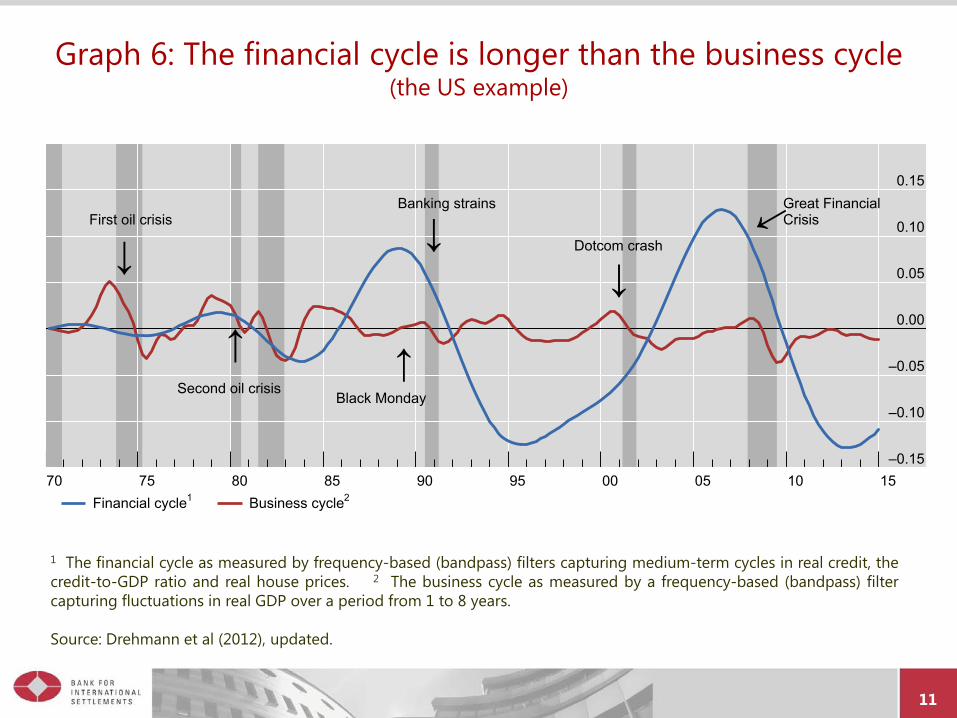
Graph 6: The financial cycle is longer than the business cycle (the US example)

1 The financial cycle as measured by frequency-based (bandpass) filters capturing medium-term cycles in real credit, thecredit-to-GDP ratio and real house prices. 2 The business cycle as measured by a frequency-based (bandpass) filtercapturing fluctuations in real GDP over a period from 1 to 8 years.

Source: Drehmann et al (2012), updated.

–0.15

–0.10

–0.05

0.00

0.05

0.10

0.15

70 75 80 85 90 95 00 05 10 15

First oil crisis

Second oil crisisBlack Monday

Banking strains

Dotcom crash

Great FinancialCrisis

Financial cycle1 Business cycle2

12

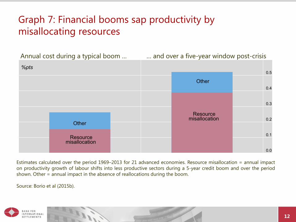
Graph 7: Financial booms sap productivity by misallocating resources

Annual cost during a typical boom … … and over a five-year window post-crisis

Estimates calculated over the period 1969–2013 for 21 advanced economies. Resource misallocation = annual impacton productivity growth of labour shifts into less productive sectors during a 5-year credit boom and over the periodshown. Other = annual impact in the absence of reallocations during the boom.

Source: Borio et al (2015b).

0.0

0.1

0.2

0.3

0.4

0.5

Other

Other

Resourcemisallocation

Resourcemisallocation

%pts

13

II – A different lens: 6 key propositions (ctd) P3: FCs have become bigger since early 1980s, following

Financial liberalisation (more ample and cheaper funding) Monetary policy frameworks focused on near-term inflation control (less resistance) Globalisation of the real economy (encourages booms, causes disinflation)

P4: The international monetary and financial system amplifies this through the interaction ofdomestic monetary and financial institutions (“regimes”) Monetary frameworks pay little attention to the build-up of FIs

- Spread easing bias from the core economies to RoW through• Extensive reach of international currencies

• Post-crisis surge of dollar credit outside the US (G 8)• Resistance to currency appreciation (policy rates kept lower/FX intervention)

• US policy rates matter beyond domestic conditions (G 9) and FX reservesballoon

Liberalised financial markets mean that- Market’s global pricing of risk and global liquidity play a key role

• External funding boosts domestic financial booms• Exchange rates overshoot

• Watch the exchange rate risk-taking channel!

14

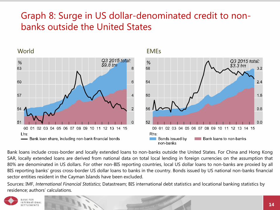
Graph 8: Surge in US dollar-denominated credit to non-banks outside the United States

Bank loans include cross-border and locally extended loans to non-banks outside the United States. For China and Hong KongSAR, locally extended loans are derived from national data on total local lending in foreign currencies on the assumption that80% are denominated in US dollars. For other non-BIS reporting countries, local US dollar loans to non-banks are proxied by allBIS reporting banks’ gross cross-border US dollar loans to banks in the country. Bonds issued by US national non-banks financialsector entities resident in the Cayman Islands have been excluded.Sources: IMF, International Financial Statistics; Datastream; BIS international debt statistics and locational banking statistics by residence; authors’ calculations.

World EMEs

15

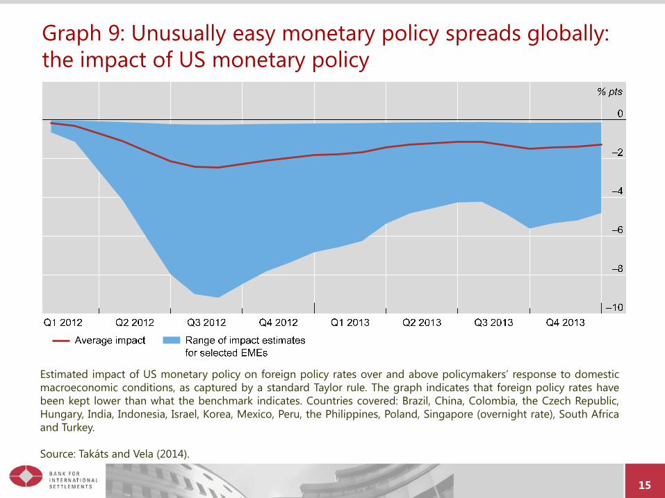
Graph 9: Unusually easy monetary policy spreads globally: the impact of US monetary policy

Estimated impact of US monetary policy on foreign policy rates over and above policymakers’ response to domesticmacroeconomic conditions, as captured by a standard Taylor rule. The graph indicates that foreign policy rates havebeen kept lower than what the benchmark indicates. Countries covered: Brazil, China, Colombia, the Czech Republic,Hungary, India, Indonesia, Israel, Korea, Mexico, Peru, the Philippines, Poland, Singapore (overnight rate), South Africaand Turkey.

Source: Takáts and Vela (2014).

16

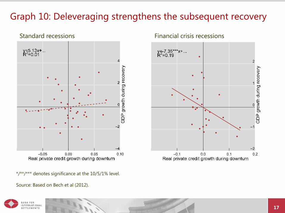
II – A different lens: 6 key propositions (ctd) P5: Post-financial boom (balance-sheet) recessions are less amenable to demand

management Less policy room for manoeuvre Less policy traction

- Deleveraging boosts subsequent recoveries (G 10)- Hence importance of balance-sheet repair and structural reforms

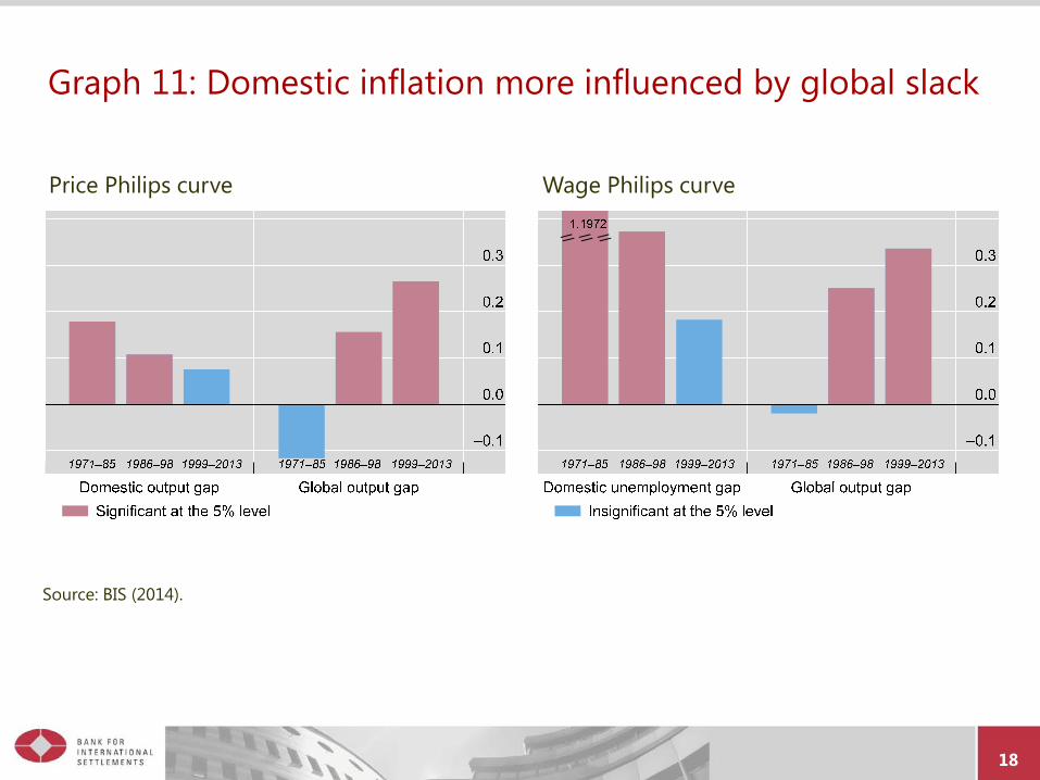
P6: Global forces have become major drivers of inflation/disinflation Well-known: link between inflation and domestic slack has been very elusive But evidence of growing role of global factors, including slack (G 11) Key role of globalisation (and possibly technological change)

- Eg, integration of China/former communist countries into global economy- Huge increase in global competition (labour & goods markets more “contestable”)

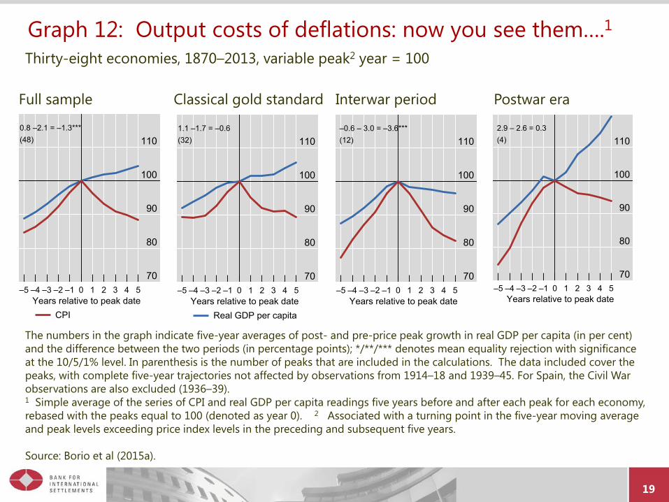
Such forces are “good”: boost output while reducing prices BIS research:

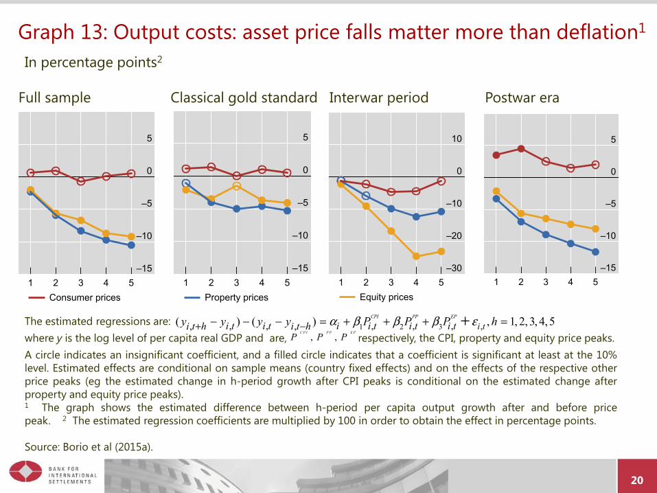
- Historically there is only a weak link between deflation and output growth (G 12)- Much stronger link with asset price declines (equity and esp property) (G 13)- No evidence of debt-deflation spirals

• But damaging interplay of debt with property price declines

17

Graph 10: Deleveraging strengthens the subsequent recovery

Standard recessions Financial crisis recessions

*/**/*** denotes significance at the 10/5/1% level.

Source: Based on Bech et al (2012).

18

Graph 11: Domestic inflation more influenced by global slack

Source: BIS (2014).// // //

Price Philips curve Wage Philips curve

19

Graph 12: Output costs of deflations: now you see them….1

The numbers in the graph indicate five-year averages of post- and pre-price peak growth in real GDP per capita (in per cent) and the difference between the two periods (in percentage points); */**/*** denotes mean equality rejection with significanceat the 10/5/1% level. In parenthesis is the number of peaks that are included in the calculations. The data included cover the peaks, with complete five-year trajectories not affected by observations from 1914–18 and 1939–45. For Spain, the Civil War observations are also excluded (1936–39).1 Simple average of the series of CPI and real GDP per capita readings five years before and after each peak for each economy, rebased with the peaks equal to 100 (denoted as year 0). 2 Associated with a turning point in the five-year moving average and peak levels exceeding price index levels in the preceding and subsequent five years.

Source: Borio et al (2015a).

Full sample Classical gold standard Interwar period Postwar era

70

80

90

100

110

–5 –4 –3 –2 –1 0 1 2 3 4 5Years relative to peak date

0.8 –2.1 = –1.3***(48)

CPI

70

80

90

100

110

–5 –4 –3 –2 –1 0 1 2 3 4 5Years relative to peak date

1.1 –1.7 = –0.6(32)

Real GDP per capita

70

80

90

100

110

–5 –4 –3 –2 –1 0 1 2 3 4 5

–0.6 – 3.0 = –3.6***

Years relative to peak date

(12)

70

80

90

100

110

–5 –4 –3 –2 –1 0 1 2 3 4 5Years relative to peak date

2.9 – 2.6 = 0.3(4)

Thirty-eight economies, 1870–2013, variable peak2 year = 100

20

Graph 13: Output costs: asset price falls matter more than deflation1

The estimated regressions are:where y is the log level of per capita real GDP and are, respectively, the CPI, property and equity price peaks.A circle indicates an insignificant coefficient, and a filled circle indicates that a coefficient is significant at least at the 10%level. Estimated effects are conditional on sample means (country fixed effects) and on the effects of the respective otherprice peaks (eg the estimated change in h-period growth after CPI peaks is conditional on the estimated change afterproperty and equity price peaks).1 The graph shows the estimated difference between h-period per capita output growth after and before pricepeak. 2 The estimated regression coefficients are multiplied by 100 in order to obtain the effect in percentage points.

Source: Borio et al (2015a).

Full sample Classical gold standard Interwar period Postwar era

In percentage points2

1 2 3 ,, , , , ,, ,( ) ( ) , 1, 2, 3, 4,5CPI PP EP

i ti t i t i i t i t i ti t h i t hy y y y P P P hα β β β ε+ −− − − = + + + =+, ,

C P I P P E P

P P P

–15

–10

–5

0

5

1 2 3 4 5Consumer prices

–15

–10

–5

0

5

1 2 3 4 5Property prices

–30

–20

–10

0

10

1 2 3 4 5Equity prices

–15

–10

–5

0

5

1 2 3 4 5

21

II – A different lens: 3 key features

Three key features distinguish the BIS lens from the prevailing one

F1: BIS lens stresses the medium term and the finance-real economy nexus The FC is a medium-term process

F2: BIS lens stresses that not all slack is born equal And hence amenable to the same remedies

F3: BIS lens stresses the importance of a global perspective As a long-term driver of disinflation In highlighting the limited insulation properties of exchange rates

22

III – A different narrative Policymakers have failed to come to grips with the FC

They did too little to constrain financial booms They relied too much on demand management to address financial busts

Drawbacks of policy most evident post-crisis As other policies lagged behind, monetary policy became overburdened Low rates in countries fighting a financial bust induced problems elsewhere

- Exchange rates took adjustment burden and appreciations elsewhere were resisted• Easing begets easing

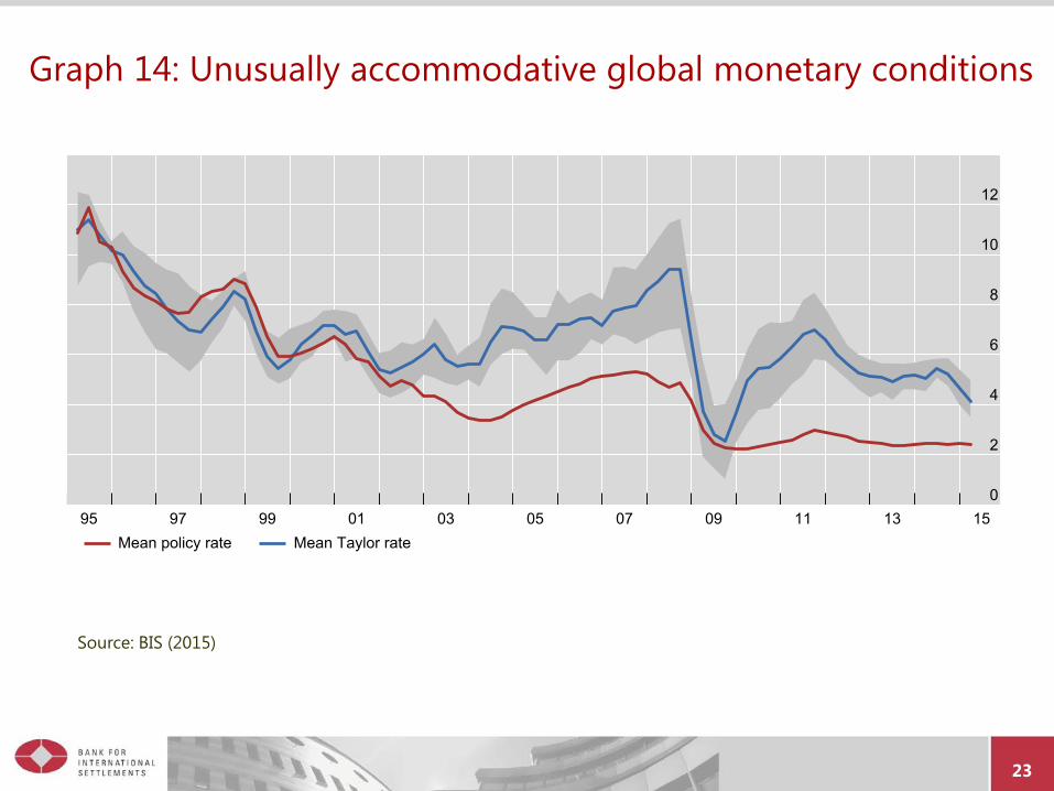
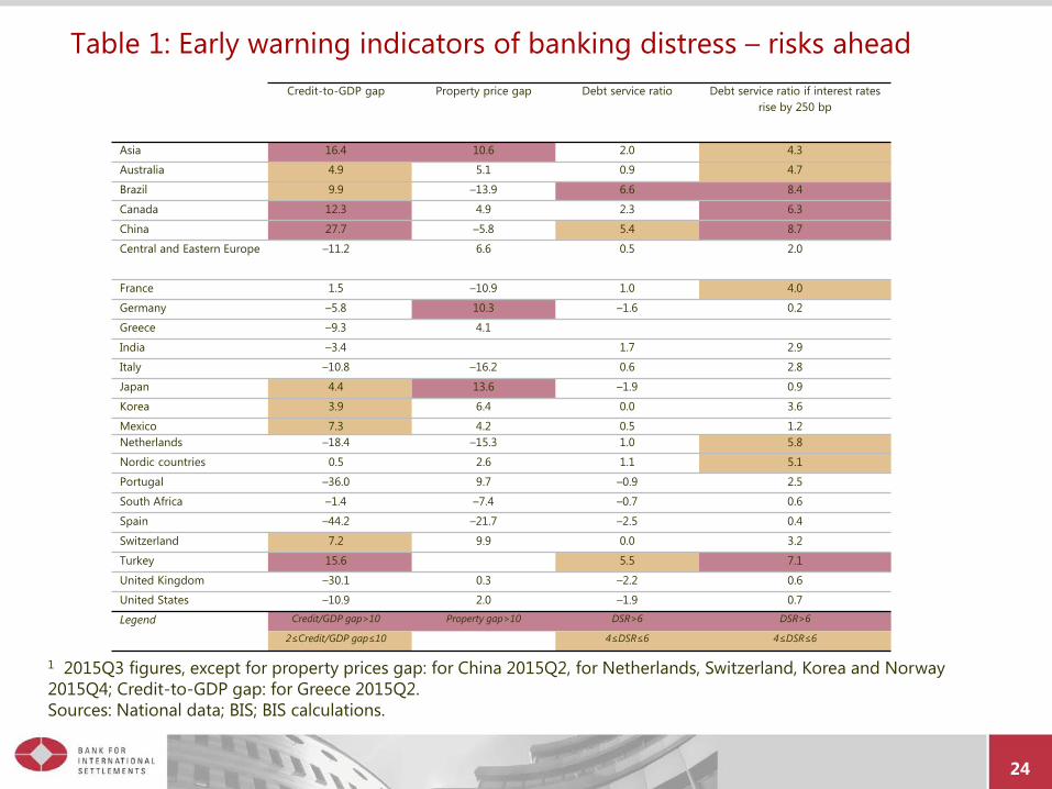
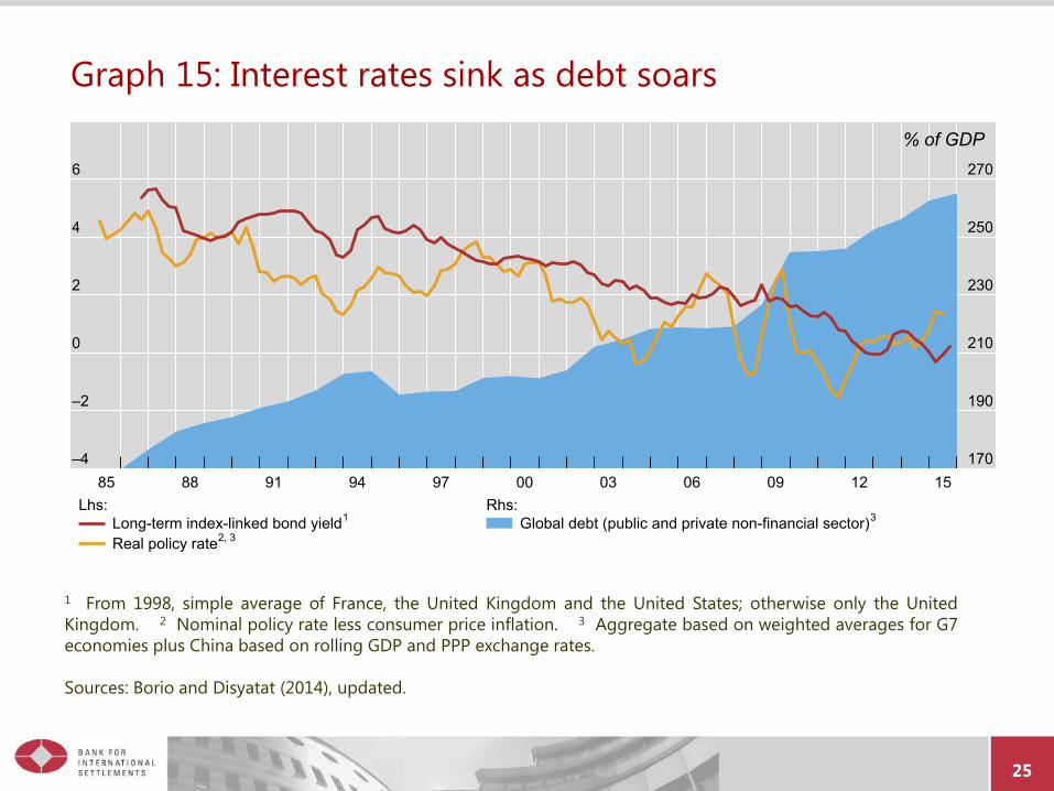
Helps explain Unusually low policy rates for the world as a whole regardless of benchmarks (G 14) Signs of the build-up of dangerous FIs in countries less affected by the crisis (T 1) Relentless rise in debt globally (G 15) Protracted slowdown; further decline in productivity growth Progressive loss in policy room for manoeuvre

Recent developments are just the latest scene in this movie Turning financial cycles in EMEs and tightening external financial conditions Risk of vicious circles, serious financial distress and weakness spreading to ROW

23

Graph 14: Unusually accommodative global monetary conditions

Source: BIS (2015)

0

2

4

6

8

10

12

95 97 99 01 03 05 07 09 11 13 15Mean policy rate Mean Taylor rate

24

Table 1: Early warning indicators of banking distress – risks aheadCredit-to-GDP gap Property price gap Debt service ratio Debt service ratio if interest rates

rise by 250 bp

Asia 16.4 10.6 2.0 4.3

Australia 4.9 5.1 0.9 4.7

Brazil 9.9 –13.9 6.6 8.4

Canada 12.3 4.9 2.3 6.3

China 27.7 –5.8 5.4 8.7

Central and Eastern Europe –11.2 6.6 0.5 2.0

France 1.5 –10.9 1.0 4.0

Germany –5.8 10.3 –1.6 0.2

Greece –9.3 4.1

India –3.4 1.7 2.9

Italy –10.8 –16.2 0.6 2.8

Japan 4.4 13.6 –1.9 0.9

Korea 3.9 6.4 0.0 3.6

Mexico 7.3 4.2 0.5 1.2Netherlands –18.4 –15.3 1.0 5.8

Nordic countries 0.5 2.6 1.1 5.1

Portugal –36.0 9.7 –0.9 2.5

South Africa –1.4 –7.4 –0.7 0.6

Spain –44.2 –21.7 –2.5 0.4

Switzerland 7.2 9.9 0.0 3.2

Turkey 15.6 5.5 7.1

United Kingdom –30.1 0.3 –2.2 0.6

United States –10.9 2.0 –1.9 0.7

Legend Credit/GDP gap>10 Property gap>10 DSR>6 DSR>6

2≤Credit/GDP gap≤10 4≤DSR≤6 4≤DSR≤6

1 2015Q3 figures, except for property prices gap: for China 2015Q2, for Netherlands, Switzerland, Korea and Norway 2015Q4; Credit-to-GDP gap: for Greece 2015Q2.Sources: National data; BIS; BIS calculations.

25

Graph 15: Interest rates sink as debt soars

1 From 1998, simple average of France, the United Kingdom and the United States; otherwise only the UnitedKingdom. 2 Nominal policy rate less consumer price inflation. 3 Aggregate based on weighted averages for G7economies plus China based on rolling GDP and PPP exchange rates.

Sources: Borio and Disyatat (2014), updated.

–4

–2

0

2

4

6

170

190

210

230

250

270

85 88 91 94 97 00 03 06 09 12 15

% of GDP

Long-term index-linked bond yield1

Real policy rate2, 3

Lhs:Global debt (public and private non-financial sector)3

Rhs:

26

Conclusion The global economy is struggling to achieve sustainable and balanced expansion

Most conspicuous sign: exceptionally low interest rates for exceptionally long Most recent slowdown in EMEs is but latest scene in a long movie

I have offered a possible lens to understand this predicament Key: inability of policy frameworks to come to grips with the global economy's… …propensity to generate hugely damaging financial booms and busts

This raises near-term and long-term risks Further episodes of serious financial distress Entrenching instability and chronic weakness A rupture in the open global economic order

Adjustments to policy frameworks are needed Address the FC through all policies (PP, MP and FP) – more symmetry is key Rebalance the policy mix towards structural measures Not presume that if one's own house is in order the global village will also be Lengthen policy horizons

We cannot afford to rely on the current debt-fuelled growth model any longer The sooner we realise this, the better

References (to BIS work only) Bank for International Settlements (2014): 84th BIS Annual Report, June ______ (2015): 85th BIS Annual Report, June Bech, M, L Gambacorta and E Kharroubi (2012): “Monetary policy in a downturn: are financial crises special?”, BIS Working Papers, no 388, September.

(published in International Finance) Borio, C (2010) : Implementing a macroprudential framework: blending boldness and realism, Capitalism and Society, vol 6 (1), Article 1. ______ (2014a): The financial cycle and macroeconomics: what have we learnt?, Journal of Banking & Finance, vol 45, pp 182–198, August. Also available

as BIS Working Papers, no 395, December 2012. —— (2014b): The international monetary and financial system: its Achilles heel and what to do about it, BIS Working Papers, no 456, September. —— (2014c): Macroprudential frameworks: (too) great expectations?, Central Banking Journal, August. Also available as BIS Speeches. —— (2014d): Monetary policy and financial stability: what role in prevention and recovery?, Capitalism and Society, Vol 9(2), Article 1. Also available as

BIS Working Papers, no 440, January. ______ (2015): Revisiting three intellectual pillars of monetary policy received wisdom, Cato Journal, forthcoming. Also available as BIS

Speeches. Borio, C and P Disyatat (2011): Global imbalances and the financial crisis: Link or no link?, BIS Working Papers, no 346, May. —— (2014): Low interest rates and secular stagnation: Is debt a missing link? , Vox EU, 25 June Borio, C, P Disyatat and M Juselius (2013): Rethinking potential output: embedding information about the financial cycle, BIS Working Papers, no 404,

February Borio, C and M Drehmann (2009): Assessing the risk of banking crises – revisited”, BIS Quarterly Review, March, pp 29–46 Borio, C, M Erdem, B Hoffman and A Filardo (2015a): The costs of deflations: a historical perspective, BIS Quarterly Review, March. Borio, C, E Kharroubi, C Upper and F Zampolli (2015b): Labour reallocation and productivity dynamics: financial causes, real consequences, BIS Working

Papers, no 534, December. Borio, C, R McCauley and P McGuire (2011): Global credit and domestic credit booms BIS Quarterly Review, September, pp 43-57 Borio, C and H Zhu (2011): Capital regulation, risk-taking and monetary policy: a missing link in the transmission mechanism?, Journal of Financial

Stability, December. Also available as BIS Working papers, no 268, December 2008. Bruno, V and H Shin (2014): Cross-border banking and global liquidity, BIS Working Papers, no 458, September. Bruno, V, I Shim and H Shin (2015): Comparative assessment of macroprudential policies, BIS Working Papers, no 502, June. Caruana (2016): Credit, commodities and currencies, Lecture at the London School of Economics and Political Science, 5 February. Drehmann, M, C Borio and K Tsatsaronis (2012): “Characterising the financial cycle: don’t lose sight of the medium term!”, BIS Working Papers, no 380,

November. Cecchetti, S and E Kharroubi (2015): Why does financial sector growth crowd out real economic growth?, BIS Working Papers, no 490, February. Drehmann, M, C Borio and K Tsatsaronis (2012): Characterising the financial cycle: don’t lose sight of the medium term!, BIS Working Papers, no 355,

November. Drehmann, M and M Juselius (2013): Evaluating early warning indicators of banking crises: Satisfying policy requirements, BIS Working Papers, no 421,

August. —— (2015): Leverage dynamics and the real burden of debt, BIS Working Papers, no 501, May. Hofmann, B and B Bogdanova (2012): Taylor rules and monetary policy: a global "Great Deviation"? BIS Quarterly Review, September, pp 37–49. Hofmann, B and E Tákats: (2015): International monetary spillovers, BIS Quarterly Review, September. McCauley, R, P McGuire and V Sushko (2015): Global dollar credit: links to US monetary policy and leverage , BIS Working Papers, no 483, January. Takáts, E and A Vela (2014): International monetary policy transmission, BIS Papers, no 78, August.

27