16. D. W. Lea, J. Clim. 17, 2170–2179 (2004).17. T. Sagawa, Y. Yokoyama, M. Ikehara, M. Kuwae, Geophys. Res.

Lett. 38, L00F02 (2011).18. P. N. DiNezio et al., Paleoceanography 26, PA3217 (2011).19. D. H. Andreasen, A. C. Ravelo, Paleoceanography 12, 395–413 (1997).20. J. Xu, W. Kuhnt, A. Holbourn, M. Regenberg, N. Andersen,

Paleoceanography 25, PA4230 (2010).21. P. Fiedler, L. Talley, Prog. Oceanogr. 69, 143–180 (2006).22. K. Thirumalai, J. W. Partin, C. S. Jackson, T. M. Quinn,

Paleoceanography 28, 401–412 (2013).23. E. C. Brady, B. L. Otto-Bliesner, J. E. Kay, N. Rosenbloom,

J. Clim. 26, 1901–1925 (2013).24. A. Patrick, R. Thunell, Paleoceanography 12, 649–657 (1997).25. H. Spero, K. Mielke, E. Kalve, D. Lea, D. Pak, Paleoceanography

18, 1022 (2003).26. D. Rincón-Martínez, S. Steph, F. Lamy, A. Mix, R. Tiedemann,

Mar. Micropaleontol. 79, 24–40 (2011).

27. H. M. Benway, A. C. Mix, B. A. Haley, G. P. Klinkhammer,Paleoceanography 21, PA3008 (2006).

28. A. Koutavas, J. Lynch-Stieglitz, T. M. Marchitto Jr., J. P. Sachs,Science 297, 226–230 (2002).

29. G. E. Manucharyan, A. V. Fedorov, J. Clim. 27, 5836–5850 (2014).30. Z.-Z. Hu et al., J. Clim. 26, 2601–2613 (2013).31. M. Collins et al., Nat. Geosci. 3, 391–397 (2010).32. N. A. Rayner et al., J. Geophys. Res. 108, 4407 (2003).

ACKNOWLEDGMENTS

We thank P. DiNezio, A. Fedorov, B. Hönisch, G. Manucharyan,A. Moore, A. Paytan, J. Zachos, and two anonymous reviewersfor comments on the manuscript. R. Franks, E. Chen,J. Hourigan, and N. Movshovitz provided analytical support.For this research, we used samples provided by the IntegratedOcean Drilling Program (IODP). Funding for this researchwas provided by NSF grant OCE-1204254 (A.C.R.), the

Achievement Rewards for College Scientists Foundation (H.L.F.),and the Schlanger Fellowship (H.L.F), which is part of theNSF-sponsored U.S. Science Support Program for IODP that isadministered by the Consortium for Ocean Leadership. Our dataare deposited at the National Oceanic and AtmosphericAdministration National Climatic Data Center and Pangaea.

SUPPLEMENTARY MATERIALS

www.sciencemag.org/content/347/6219/255/suppl/DC1Materials and MethodsSupplementary TextFigs. S1 to S17Tables S1 to S3References (33–70)

7 July 2014; accepted 11 December 201410.1126/science.1258437

PALEOECOLOGY

Linked canopy, climate, and faunalchange in the Cenozoic of PatagoniaRegan E. Dunn,1* Caroline A. E. Strömberg,1 Richard H. Madden,2

Matthew J. Kohn,3 Alfredo A. Carlini4

Vegetation structure is a key determinant of ecosystems and ecosystem function, butpaleoecological techniques to quantify it are lacking.We present a method for reconstructing leafarea index (LAI) based on light-dependent morphology of leaf epidermal cells and phytolithsderived from them. Using this proxy, we reconstruct LAI for the Cenozoic (49 million to 11 millionyears ago) of middle-latitude Patagonia. Our record shows that dense forests opened up by thelate Eocene; open forests and shrubland habitats then fluctuated, with a brief middle-Mioceneregreening period. Furthermore, endemic herbivorous mammals show accelerated tooth crownheight evolution during open, yet relatively grass-free, shrubland habitat intervals. Our PatagonianLAI record provides a high-resolution, sensitive tool with which to dissect terrestrial ecosystemresponse to changing Southern Ocean conditions during the Cenozoic.

Vegetation structure—the degree of canopyopenness—is a fundamental aspect of eco-systems, influencing productivity, hydro-logical and carbon cycling, erosion, andcomposition of faunal communities (1, 2).

However, methods to quantify ancient vegeta-tion structure have eluded paleoecologists. Here,we present a method with which to reconstructvegetation openness, specifically leaf area index[LAI = foliage area (m2)/ground area (m2)], using

the morphology of leaf epidermal cells preservedas phytoliths (plant biosilica) (Fig. 1). LAI quan-tifies vegetation structure in ecological andclimate modeling studies (1, 3). In modern eco-systems, LAI relates primarily to soil moisture(4), by which vegetation becomes more closed withincreasing soil water availability; ultimately, soilmoisture is determined by temperature, precipi-tation, and atmospheric partial pressure of CO2

(PCO2) (4, 5). Disturbance in the form of fire andherbivory can offset this relationship, resultingin open habitats in areas with relatively highrainfall (6).Using this paleobotanical archive, we re-

constructed a LAI record for the middle Ceno-zoic [49 million to 11 million years ago (Ma)] ofPatagonia to test predictions about vegetation

258 16 JANUARY 2015 • VOL 347 ISSUE 6219 sciencemag.org SCIENCE

Fig. 1. Leaf epidermis and examples of epidermal phytoliths. (A) Nothofagus leaf and epidermis. (B to E) Fossil phytoliths from Patagonia. (F to I)Modern soil phytoliths from Costa Rica.

1Department of Biology and Burke Museum of NaturalHistory and Culture, University of Washington, Seattle, WA98195, USA. 2Department of Organismal Biology andAnatomy, University of Chicago, Chicago, IL 60637, USA.3Department of Geosciences, Boise State University, Boise,ID 83725, USA. 4Paleontología de Vertebrados, UniversidadNacional de La Plata, Consejo Nacional de InvestigacionesCientíficas y Técnicas (CONICET), La Plata, Argentina.*Corresponding author. E-mail: dunnr@u.washington.edu

RESEARCH | REPORTS

on

Janu

ary

15, 2

015

ww

w.s

cien

cem

ag.o

rgD

ownl

oade

d fr

om

on

Janu

ary

15, 2

015

ww

w.s

cien

cem

ag.o

rgD

ownl

oade

d fr

om

on

Janu

ary

15, 2

015

ww

w.s

cien

cem

ag.o

rgD

ownl

oade

d fr

om

on

Janu

ary

15, 2

015

ww

w.s

cien

cem

ag.o

rgD

ownl

oade

d fr

om

response to Cenozoic climate fluctuations andhow changes in vegetation structure relate tothe evolution of high-crowned (hypsodont) andever-growing (hypselodont) tooth morphologiesin South American herbivores (7).Climatic cooling beginning in the middle

Eocene (49 Ma) and major warming events inthe late Oligocene (~26 Ma) and middle Miocene(17 to 14 Ma) (8) have been linked to tectonics,ocean circulation (9), atmospheric PCO2 (10), andice volume after the onset of extensive Antarctic

glaciation at the Eocene–Oligocene Transition(EOT; 33.9 Ma) (8). A narrow landmass, Pata-gonia is sensitive to Southern Ocean climate andprovides an ideal test case for the influence ofglobal climate on vegetation structure.It has long been assumed that hypsodonty in

endemic South American herbivores beginningin the middle Eocene (~40 Ma) evolved in re-sponse to the spread of Earth’s first grasslands(11), but recent work found that grasses were rare(12). When grasses are rare, “traditional” phyto-

lith analysis cannot resolve habitat openness(13, 14), so it has remained unclear whether hypso-donty evolved in forests or in open but grass-freehabitats, possibly in conjunction with tooth abra-sion during ingestion of exogenous grit (12).Our proxy for reconstructing ancient LAI

[reconstructed LAI (rLAI)] is based on the well-known influence of sunlight on the size andshape of pavement cells in leaf epidermis (Fig.1A). In shade, these cells are larger and havemore undulated outlines than those of cells ex-posed to full sun (15, 16). Silica mineralizationproduces a precision cast of pavement cells inliving plants that can be preserved as fossils(Fig. 1B). Because sunlight filtering through acanopy is a function of LAI, we hypothesizedthat leaf epidermal cells and their phytoliths areon average larger and more undulated in closedforests than in open habitats and that the rela-tionship is linear across a canopy density gradient.Because these phytolith types are taxonomicallynondiagnostic we cannot control for phyloge-netic variation in cell morphology. Instead, wetested our hypotheses using modern assemb-lages of phytoliths extracted from soils collectedacross an LAI gradient from 0 (completely open)to 5 (dense forest) in Costa Rica (Fig. 1C).Cenozoic-aged floras from Patagonia con-

tain a nonanalog mix of mesic and xeric taxaof tropical and sub-Antarctic lineages (suchas Arecaceae, Anacardiaceae, Fabaceae, Zingi-beraceae, Proteaceae, Nothofagus, Podocarpa-ceae, and Araucariaceae). We chose to samplephytoliths from modern tropical soils in CostaRica because it has wet and dry forests, sa-vanna, and shrubby areas containing many ofthe reported fossil genera (41%) and families(85%) (table S1). We assume that relative changein epidermal cell morphology is based on can-opy density and is independent of taxonomyand latitudinal variation in light regime. Usinglight microscopy, nongrass epidermal phytolithsin extracted samples were photographed andmeasured for the calibration data set. Phyto-lith undulation was standardized by using anundulation index (UI = circumference of cell/circumference of a circle with cell area) (16), andmean site values for phytolith UI (PUI) andphytolith area (PA) were compared with fieldmeasurements of LAI from hemispherical pho-tographs (Fig. 2A). Measurements of fossil phy-toliths followed the same protocol.In the modern training data set of 45 sites

(table S2), LAI correlates with PUI [coefficientof determination (R2) = 0.59, P < 0.0001] (Fig.2B) and PA (R2 = 0.44, P < 0.0001) (Fig. 2C). Alinear multiple regression analysis including bothvariables improves the correlation (Fig. 2D andtable S3):

rLAI = 0.0012 × PA(mm2) + 10.4118 ×PUI – 13.1621 (1)

(R2 = 0.63, P < 0.0001, SE = 0.695, F2,42 = 39).Using Eq. 1, we reconstructed rLAI for 46 fos-sil phytolith assemblages from Patagonian paleo-sols spanning 49 to 11 Ma (Fig. 3A, fig. S3, and

SCIENCE sciencemag.org 16 JANUARY 2015 • VOL 347 ISSUE 6219 259

Fig. 2. Modern soil phytolith morphology and LAI. (A) Hemispherical photographs from CostaRica illustrating LAI values. (B) Linear regressions for mean PUI and LAI (rLAI = 13.92 × PUI – 17.31);and (C) mean Phytolith Area (PA) and LAI (rLAI = 0.0028 × PA + 0.531). (D) Plot of simulated versusmeasured values of LAI. Simulated values are derived from Eq. 1.

RESEARCH | REPORTS

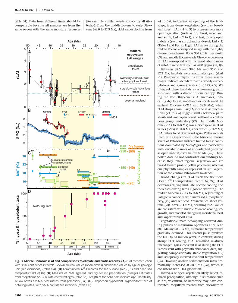
table S4). Data from different times should becomparable because all samples are from thesame region with the same moisture resources

(for example, similar vegetation occupy all sitestoday). From the middle Eocene to early Oligo-cene (49.0 to 32.3 Ma), rLAI values decline from

~4 to 0.6, indicating an opening of the land-scape, from dense vegetation (such as broad-leaf forest; LAI = 4 to 3) to progressively moreopen vegetation (such as dry forest, woodland,and scrub; LAI = 2 to 1); and last, to very openhabitats (such as shrubland or desert; LAI < 1)(Table 1 and Fig. 3). High rLAI values during themiddle Eocene correspond in age with the highlydiverse megathermal floras 380 km farther north(17), and middle Eocene–early Oligocene decreasesin rLAI correspond with increased abundancesof sub-Antarctic taxa such as Nothofagus (18, 19).Between 38.5 and 38.0 Ma and 35.0 and

32.2 Ma, habitats were maximally open (rLAI<1). Diagnostic phytoliths from these assem-blages indicate abundant palms, woody eudico-tyledons, and sparse grasses (<1 to 15%) (12). Weinterpret these habitats as a nonanalog palmshrubland with a discontinuous canopy. Dur-ing the late Oligocene, rLAI increases, indi-cating dry forest, woodland, or scrub until theearliest Miocene (~21.1 and 18.8 Ma), whenrLAI drops again. Early Miocene rLAI fluctua-tions (<1 to 2.4) suggest shifts between palmshrubland and open forest without a contin-uous grassy understory (12). The middle Mio-cene (~15.7 to 14.6 Ma) saw a brief spike in rLAIvalues (>3.5) at 14.6 Ma, after which (~14.2 Ma)rLAI values trend downward again. Pollen recordsfrom late Oligocene–middle Miocene marinestrata of Patagonia indicate humid forest condi-tions dominated by Nothofagus and podocarps,with low abundances of arid-adapted (inferredas open habitat) taxa before 10 Ma (20). Thesepollen data do not contradict our findings be-cause they reflect regional vegetation and arebiased toward prolific pollen producers, whereasour phytolith samples represent in situ vegeta-tion of the central Patagonian lowlands.Broad changes in rLAI track the Southern

Ocean d18O temperature record (8, 21); rLAIdecreases during mid–late Eocene cooling andincreases during late Oligocene warming. Themiddle Miocene (~15.7 to 14.6 Ma) regreening ofPatagonia coincides with increased atmosphericPCO2 (22) and reduced Antarctic ice sheet vol-ume (23). After ~14.2 Ma, declining rLAI valuesare consistent with middle Miocene cooling, ice-growth, and modeled changes in meridional heatand vapor transport (24).Vegetation-climate decoupling occurred dur-

ing pulses of maximum openness at 38.5 to38.0 Ma and at ~35 Ma, as marine temperaturesgradually declined. This second pulse predatesthe EOT by >1 million years; in contrast, duringabrupt EOT cooling, rLAI remained relativelyunchanged. Quasi-constant rLAI during the EOTis consistent with phytolith abundance data, sug-gesting compositionally stable vegetation (12)and isotopically inferred invariant temperatures(25). However, aeolian sedimentation rates dra-matically increased at 33.6 Ma (26), which isconsistent with Oi-1 glaciation.Intervals of open vegetation likely reflect re-

duced precipitation, although disturbance suchas fire, volcanism, or herbivory may have con-tributed. Megafloral records from elsewhere in

260 16 JANUARY 2015 • VOL 347 ISSUE 6219 sciencemag.org SCIENCE

% h

ypso

& h

ypse

lod

on

t ta

xarL

AI

Age (Ma)Eocene Oligocene Miocene

E Middle Late Late Middle LEarly Early

Notoungulata

Mi-1Oi-1 Mi-1a

15 20 25 30 35 40 45 50 10

MA

T (

ºC)

Age (Ma)

scrub/dry sclerophyllous forest

broadleaved forest

Nothofagus decid./ wet sclerophyllous forest

desert/shrubland

Modern ecosystem LAI ranges

δ18O

(‰

)

0

1

2

3

15 20 25 30 35 40 45 50 10

RT

NM

BP

LL

RP

NI

RT

NM

BP

LL

RP

NI

18

22

Megafloral climate reconstructions

paleosol MAP

EOT

16

LOWE MMCOMECO

MMCT

G

LA

250 (60)

50 (20)

150 (40)

Precip

itation

(cm/yr)

MAP Dry Season

26

0

1

2

3

4

5

0

50

100

Fig. 3. Middle Cenozoic rLAI and comparisons to climate and biotic records. (A) rLAI reconstructionwith 95% confidence intervals. Shown are raw values (open circles) and binned values by age or geologicunit (red diamonds) (table S4). (B) Foraminiferal d18O records for sea surface (red) (21) and deep seatemperature (blue) (8). (C) MAT (blue), MAP (green), and dry-season precipitation (orange) estimatesfrom megafloras (27, 33), with corrected ages (table S5). Length of the solid bars indicate age uncertainty.Yellow boxes are MAP estimates from paleosols (34). (D) Proportion hypsodont+hypselodont taxa ofnotoungulates, with 95% confidence intervals (table S6).

RESEARCH | REPORTS

Patagonia document stable mean annual tem-peratures (MATs) of ~18°C, but decreasing meanannual precipitation (MAP) from the middleEocene onward (Fig. 3C) (27). By at least thelate Oligocene, decreased MAP values reflect re-duced dry-season rainfall (27). Locally, episodesof low rLAI correspond to the lowest MAP es-timates from paleosols and shifts to aeoliansedimentation (28). Additionally, phytoliths ofwater-demanding gingers become very rare (0.4%)by 38.1 Ma and disappear after ~38 Ma (12).Our climate interpretation is seemingly at oddswith phytolith evidence for abundant palms,which in modern South America is linked towarm, humid climates (29). However, Patago-nian fossils indicate that a largely dry-adaptedpalm clade (Attaleinae) had diversified in SouthAmerica by the Paleocene (fig. S5). We hypoth-esize that water-use efficiency in these palmswas further enhanced under elevated Eocene at-mospheric PCO2 (30).Increasing openness (rLAI < 1) ~40 Ma co-

incided with initiation of tooth crown heightincreases in several clades of notoungulates (Fig.3D). Proportions of hypsodont+hypselodont taxacontinued to rise from 38 to 20 Ma, as rLAIremained low (between 0 and 2; average ≤ 1.5).The hypsodonty trend may have reversed dur-ing more forested middle Miocene conditions,but errors are large, and constant hypsodontyproportions cannot be ruled out. In modernSouth American environments, the proportionof hypsodont+hypselodont species dramaticallyincreases under a LAI value of ~1.2 (fig. S6 andtable S7). These areas experience low precipi-tation, frequent dust storms, and erosion oftephric materials (31).Evidently, feeding in drier, more open Eocene–

early Miocene ecosystems provided evolutionarypressure to drive hypsodonty and hypselodontyin Patagonia. The temporal coincidence of wind-blown ash, low rLAI, and increased rates ofhypsodonty+hypselodonty further suggests thatash played a key role in this process (12). In low

LAI habitats today (such as shrublands), sparsevegetation includes both bare ground (dustsource areas) and shrubs (traps for dust) (32).Thus, ingestion of dust adhering to plants growingon highly erodible surfaces (tephra-rich soils)plausibly drove this pattern of tooth evolutionin South America.Taken together, these patterns indicate that

long-term climate changes that predated theEOT drove ecosystem changes in Patagonia.Specifically, we propose that Southern Oceaninstability during the protracted opening ofDrake Passage beginning in the middle Eocene(9) and associated cooling sea surface temper-atures resulted in reduced rainfall on land andtriggered successive opening-up of landscapesduring the middle-late Eocene. Our methodfor estimating rLAI allows for quantificationof vegetation structure through time, and be-cause it relies on microfossils, extremely high-resolution records of habitat change are possible.Additionally, because leaf epidermis is a high-ly conserved tissue, the method should beapplicable across a broad range of temporalscales to test many outstanding hypotheses inpaleoecology.

REFERENCES AND NOTES

1. G. P. Asner, J. M. O. Scurlock, J. A. Hicke, Glob. Ecol. Biogeogr.12, 191–205 (2003).

2. R. F. Kay, R. H. Madden, C. Van Schaik, D. Higdon, Proc. Natl.Acad. Sci. U.S.A. 94, 13023–13027 (1997).

3. R. Betts, P. Cox, S. Lee, F. Woodward, Nature 387, 796–799(1997).

4. O. Dermody, J. F. Weltzin, E. C. Engel, P. Allen, R. J. Norby,Plant Soil 301, 255–266 (2007).

5. A. Iio, K. Hikosaka, N. P. R. Anten, Y. Nakagawa, A. Ito, Glob.Ecol. Biogeogr. 23, 274–285 (2013).

6. A. C. Staver, S. Archibald, S. A. Levin, Science 334, 230–232(2011).

7. Materials and methods are available as supplementarymaterials on Science Online.

8. J. Zachos, M. Pagani, L. Sloan, E. Thomas, K. Billups, Science292, 686–693 (2001).

9. R. Livermore, C.-D. Hillenbrand, M. Meredith, G. Eagles,Geochem. Geophys. Geosyst. 8, Q01005 (2007).

10. M. Pagani, J. C. Zachos, K. H. Freeman, B. Tipple, S. Bohaty,Science 309, 600–603 (2005).

11. B. F. Jacobs, J. D. Kingston, L. L. Jacobs, Ann. Mo. Bot. Gard.86, 590–643 (1999).

12. C. A. E. Strömberg, R. E. Dunn, R. H. Madden, M. J. Kohn,A. A. Carlini, Nat. Commun. 4, 1478 (2013).

13. C. A. E. Strömberg, Palaeogeogr. Palaeoclimatol. Palaeoecol.207, 239–275 (2004).

14. L. Bremond, A. Alexandre, C. Hély, J. Guiot, Global Planet.Change 45, 277–293 (2005).

15. R. W. Watson, New Phytol. 41, 223–229 (1942).16. W. M. Kürschner, Rev. Palaeobot. Palynol. 96, 1–30 (1997).17. P. Wilf et al., Am. Nat. 165, 634–650 (2005).18. V. Barreda, L. Palazzesi, Bot. Rev. 73, 31–50 (2007).19. E. J. Romero, Ann. Mo. Bot. Gard. 73, 449–461 (1986).20. L. Palazzesi, V. Barreda, Nat. Commun. 3, 1294 (2012).21. S. M. Bohaty, J. C. Zachos, Geology 31, 1017–1020 (2003).22. Y. G. Zhang, M. Pagani, Z. Liu, S. M. Bohaty, R. Deconto,

Philos. Trans. A Math. Phys. Eng. Sci. 371, 20130096(2013).

23. S. Warny et al., Geology 37, 955–958 (2009).24. A. E. Shevenell, J. P. Kennett, D. W. Lea, Science 305,

1766–1770 (2004).25. M. J. Kohn et al., Geology 32, 621 (2004).26. R. E. Dunn et al., Geol. Soc. Am. Bull. 125, 539–555

(2013).27. L. Hinojosa, Rev. Geológica Chile 32, 95–115 (2005).28. E. S. Bellosi, in The Paleontology of Gran Barranca: Evolution

and Environmental Change Through the Middle Cenozoic ofPatagonia, R. H. Madden, A. A. Carlini, M. G. Vucetich,R. F. Kay, Eds. (Cambridge Univ Press, Cambridge, UK, 2010),pp. 278–292.

29. S. W. Punyasena, Palaeogeogr. Palaeoclimatol. Palaeoecol. 265,226–237 (2008).

30. M. H. Ibrahim, H. Z. E. Jaafar, M. H. Harun, M. R. Yusop, ActaPhysiol. Plant. 32, 305–313 (2009).

31. R. H. Madden, Hypsodonty in Mammals: Evolution,Geomorphology and the Role of Earth Surface Processes(Cambridge Univ. Press, Cambridge, UK, 2014).

32. D. D. Breshears, J. J. Whicker, M. P. Johansen, J. E. Pinder,Earth Surf. Process. Landf. 28, 1189–1209 (2003).

33. L. F. Hinojosa, C. Villagrán, Palaeogeogr. Palaeoclimatol.Palaeoecol. 217, 1–23 (2005).

34. E. S. Bellosi, M. G. Gonzalez, in The Paleontology of GranBarranca: Evolution and Environmental Change through theMiddle Cenozoic of Patagonia, R. H. Madden, A. A. Carlini,M. G. Vucetich, R. F. Kay, Eds. (Cambridge Univ. Press, 2010),pp. 293–305.

35. S. Ganguly et al., Remote Sens. Environ. 112, 4318–4332(2008).

36. E. Gutiérrez, V. Vallejo, Oecologica Aquat. 10, 351–366(1991).

37. W. Woodgate, Int. Arch. Photogramm. Remote Sens. Spat. Inf.Sci. XXXIX, 457–462 (2012).

38. G. P. Asner, C. E. Borghi, R. A. Ojeda, Ecol. Appl. 13, 629–648(2003).

39. M. Barradas, F. Novo (Folia Geobot. Phytotaxon. 22, 415–433(1987).

40. V. Barraza et al., IEEE J. Sel. Top. Appl. Earth Obs. RemoteSens. 7, 421–430 (2013).

ACKNOWLEDGMENTS

Supplementary data are included in the data file. This research wasfunded in part by National Science Foundation grants DEB-1110354 toR.E.D. and C.A.E.S. (Doctoral Dissertation Improvement Grant) andEAR-0819910 to C.A.E.S., EAR-0819842 to R.H.M., and EAR-0819837and EAR-1349749 to M.J.K.; Proyecto de Investigación en Ciencias yTécnicas 1860 of the Fondo Nacional de Ciencia y Tecnología(FONCyT) To A.A.C.; the Geological Society of America; and theUniversity of Washington Department of Biology and Burke Museumof Natural History and Culture. We thank G. Vucetich, M. Ciancio,M. Conner, A. Loeser, Pan American Energy, Organization forTropical Studies, Área Conservación de Guanacaste, and threereviewers.

SUPPLEMENTARY MATERIALS

www.sciencemag.org/content/347/6219/258/suppl/DC1Materials and MethodsFigs S1 to S6Tables S1 to S6References (41–62)

8 September 2014; accepted 9 December 201410.1126/science.1260947

SCIENCE sciencemag.org 16 JANUARY 2015 • VOL 347 ISSUE 6219 261

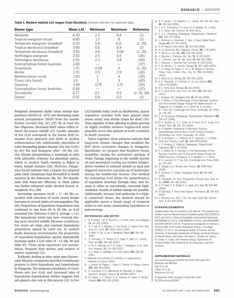
Table 1. Modern habitat LAI ranges from literature. Dashes indicate no reported data.

Biome type Mean LAI Minimum Maximum Reference

Wetlands 6.30 2.5 8.4 (1)Tropical evergreen broad 4.80 1.5 8 (1)Temperate evergreen broadleaf 4.33 0.8 11.6 (1, 35)Tropical deciduous broadleaf 3.90 0.6 8.9 (1)Temperate deciduous broadleaf 3.56 0.6 5.08 (1, 35)Nothofagus evergreen 3.50 2.5 4.5 (36)Nothofagus deciduous 2.55 2.3 2.8 (36)Sclerophyllous forest Australia 2.40 — — (37)Grasslands 1.75 0.08 5 (1, 35)Monte 1.70 0.5 2.9 (38)Mediterranean scrub 1.50 1 4 (39)Chaco (dry forest) 1.5 1 3 (40)Savanna 1.49 0.78 1.72 (35)Sclerophyllous forest Australia 0.95 — — (37)Shrublands 0.77 0.1 4.5 (1, 35, 38)Desert 0.55 0.9 0.2 (1)

RESEARCH | REPORTS