the moderating e ects of marriage across party lines · the moderating e ects of marriage across...

The Moderating Effects of Marriage Across Party Lines

Shanto Iyengar∗ Tobias Konitzer†

∗Stanford University [email protected]†Stanford University [email protected]

1

“The Democrats, wherever you find ’em – in the media, think tanks, don’t care whereyou find ’em – they’re being consumed by it, folks. Theyre literally being eaten alive withan irrational, raw hatred.” – Rush Limbaugh, May 10, 2017.

In the aftermath of the 2016 election, the American electorate is hyperpolarized. Animus

toward the out party is at an historic high. For the first time on record, the most frequently

registered feeling thermometer score for the opposing party (e.g. Democrats’ rating of the

Republican Party and vice-versa) in the 2016 American National Election Study was at the

minimum, i.e. zero. Other indicators are similarly skewed toward the extremes. President

Trump’s approval drops precipitously from 80 percent among Republicans to under ten

percent for Democrats. Some six times as many Democrats than Republicans believe that

the Trump campaign colluded with the Russians to sway the election (Washington Post Poll,

April 26, 2017).

Hostility directed at out groups is a fundamental barometer of group polarization. Classic

studies on social distance (Bogardus, 1925), and the sense of social identity (Tajfel, 1970;

Tajfel and Turner, 1979) have established that diverging sentiment for in- and out-group

members is inevitable. Group polarization defined in terms of differential affect for the in

and out group occurs even when the basis for group affiliation is trivial and completely

unrelated to group interests.

In the context of American politics, affective polarization deriving from political party

affiliation is well documented, in stark contrast to ideological polarization, where the evidence

is mixed (compare Abramowitz 2010 with Fiorina, Abrams and Pope 2005). As for partisan

affect, data from the American National Election Surveys dating to the mid-1980s shows

that Democrats and Republicans not only increasingly dislike the opposing party, but also

impute negative qualities to its supporters (Iyengar, Sood and Lelkes, 2012).

Out-group prejudice based on party identity exceeds the comparable bias directed at

racial, religious, or cultural out groups (Muste, 2014; Iyengar and Westwood, 2015). Partisan

2

affect has strengthened to the point where party identity is now a litmus test for interpersonal

attraction. People prefer to associate with fellow partisans and are less trusting of partisan

opponents (Iyengar and Westwood, 2015; Westwood et al., 2017). The most vivid evidence

of increased social distance across the party divide concerns inter-party marriage. In the

early 1960s, the percentage of partisans expressing concern over the prospect of their son

or daughter marrying someone from the opposition party was in the single digits, but some

forty-five years later it had risen to more than twenty-five percent (Iyengar, Sood and Lelkes,

2012).

Data from surveys of married couples, online dating sites, and national voter files confirm

that partisanship has become a key attribute underlying the selection of long-term partners

(Huber and Malhotra, 2017; Iyengar, Konitzer and Tedin, 2017). Among recently married

couples in 1973, only 54 percent shared the same party affiliation. Forty years later, partisan

agreement among this group had risen to 74 percent (Iyengar, Konitzer and Tedin, 2017).

Survey results standing alone may not be the most meaningful measure of increasing

partisan animus. The expression of hostility based on partisanship is not subject to the

same social taboos as hostility based on other salient social divides (racial, religious, or

ethnic). Instead, hostility directed at the out party is deemed acceptable, even appropriate.

Therefore, survey data could artificially elevate the significance of the partisan divide over

other significant cleavages. But, importantly, there is considerable evidence of increased

partisan animus outside the survey realm; this evidence is not subject to normative, conscious

restraints based on political correctness. Using a version of the Implicit Association Test,

Iyengar and Westwood (2015) demonstrated that implicit bias directed at the out party

exceeded comparable bias based on race. They also showed that behavioral discrimination

against partisan opponents in a variety of contexts exceeded discrimination based on other

group cues, most notably, race.

What explains the dramatic increase in affective polarization over the past few decades?

3

The period in question (1985 - 2015) coincides with any number of major societal changes,

including the vastly increased ethnic and cultural diversity of the population, the migration of

whites from urban areas to the suburbs, the emergence of the South as a staunch Republican

region, and the politicization of evangelical Christians. One possible explanation, sometimes

referred to as ”sorting,” is the increasing convergence of multiple salient social identities

which reinforce each other. In other words, Democrats and Republicans differ not only in

their politics, but also in their ethnic, religious, gender, cultural, and regional identities.

Sorting leads to overlapping group memberships and the increasing partisan homogene-

ity of primary and secondary groups is a further contributor to polarization. Family and

kinship networks – key influences over the development of political attitudes – provide few

opportunities for meaningful and long-term personal contact across party lines. As we note

below, even at the level of secondary groups, defined on the basis of occupation, religion, or

place of residence, partisan homophily is extensive (for evidence on occupational similarity in

partisan affiliation, see Bonica, Chilton, and Sen 2016; the geographic sorting of the nation

into Republican and Democratic enclaves is documented most recently in Chen and Cottrell

2016 and Chen, Rodden et al. 2013.

We investigate the role of interpersonal relations as a potential contributor to partisan

polarization. We focus on the family, the most important agent of political socialization.

Comparing surveys of spouses conducted in the 1960s, the 1990s and the current era, we

demonstrate that over time, spousal disagreement – although clearly becoming less frequent

– can act as a brake on polarization by fostering less hostile attitudes toward partisan op-

ponents. The more heterogeneous the household, the less polarized the individual members.

We replicate these survey findings a secondary analysis of a set of 2015 and 2016 field exper-

iments that targeted registered voters in multiple states. Participants in these experiments

completed surveys that included feeling thermometers and other measures of partisan affect.

Because the surveys sampled multiple family members living at the same address, we can

4

investigate the effects of household agreement on partisan affect. In fact, the data from these

field studies converge with the surveys of spouses; mixed-party households are significantly

less polarized.1

Household Diversity as a De-Polarizing Influence

Decades of research into group dynamics and social influence shows that people are at-

tracted to similar others creating pressures toward group homogeneity (McPherson, Smith-

Lovin and Cook, 2001). Groups based on strong ties such as kinship are especially homoge-

neous, but in recent years the pattern also extends to secondary groups based on relatively

weak ties including acquaintanceship, shared occupation or place of residence (see DiPrete

and Jennings, 2012; Skocpol, 2013; Putnam, 2001). Thus, interpersonal contact typically

occurs within a non-diverse political environment.

The composition of social networks exerts powerful downstream effects on attitudes and

group polarization. For one thing, the more homogeneous and dense the network, the

more one-sided the stream of information, thus reinforcing group members’ prior sentiments

(Schkade, Sunstein and Hastie, 2010; Sunstein and Hastie, 2015). When the group consists

disproportionately of whites, their attitudes toward racial minorities become more stereo-

typic; discussion among men elicits sexist views, and so on (Baldassarri and Bearman, 2007;

Bienenstock, Bonacich and Oliver, 1990). Group homogeneity instills polarization as mem-

bers gravitate toward pro-in group and anti-out group positions, so much so that in formal

models of group formation, homogeneous, polarized groups represent the ”stable equilibrium

outcome” (Axelrod, 1997; Abelson, 1979).

There is also evidence of the opposite pattern corresponding to groups that are diverse.

Diversity of social ties creates ”cross pressures” that lead individuals to take on positions that

are not perfectly aligned with their group interests. The more heterogeneous the composition

1We are indebted to David Broockman and Joshua Kalla for bringing these data to our attention andfor generously providing access.

5

of the group, the more tolerant group members toward oppositional viewpoints, the more

aware individuals of the perspectives taken by their opponents, and the less prejudiced their

views of out groups (Mutz, 2002, 2006; Pettigrew, 1990; Pettigrew and Tropp, 2000; Brown

and Hewstone, 2005; Sheagley, forthcoming). From this perspective, group disagreement

ameliorates polarization.

As indicated above, one reason group membership proves polarizing is that individuals

are exposed to one-sided streams of communication. Individuals unfamiliar with the group

gestalt learn their appropriate lines. In addition to facilitating persuasion, groups may

influence attitudes by inducing conformity motivated by individuals’ desire to fit in and gain

group acceptance (Katz and Lazarsfeld, 1955; Lazarsfeld, Berelson and Gaudet, 1948; Asch

and Guetzkow, 1951).

In the case of party preference, the evidence on group homogeneity is mixed. On the one

hand, at the level of the family, there is strong evidence of convergence between spouses and

across generations (Jennings and Niemi, 1974; Jennings, Stoker and Bowers, 2009; Rico and

Jennings, 2016). The longitudinal studies show increased family homogeneity in the current

era, and increased inter-generational correspondence (Iyengar, Konitzer and Tedin, 2017).

More importantly, this work demonstrates that spousal political agreement is not a byprod-

uct of marital selection on some non-political attribute that is related to partisanship (e.g.

economic status). Rather the selection mechanism is overtly political; it is the individuals’

politics that drives marital attraction (see Huber and Malhotra, 2017; Iyengar, Konitzer and

Tedin, 2017, pp.19-21).

When we turn from the primary group to groups based on weak ties, however, evidence

of partisan homogeneity is more ambiguous. Networks consisting of people who talk about

politics, for instance, are characterized by considerable variability in party affiliation. In

a study conducted during the 2000 presidential election, despite the relatively polarizing

campaign and ensuing litigation over the disputed outcome, more than 50 percent of the

6

respondents in a national survey who identified the individuals with whom they discussed

politics (as well as their political views) were embedded in discussion networks that included

at least one individual not from the respondent’s preferred party (Huckfeldt, Johnson and

Sprague, 2004, 2002). Beyond the family, encounters with political disagreement may not

be a rare outcome.

One location thought to provide regular opportunities for interactions across the political

divide is the workplace (Mutz, 2006; Mutz and Mondak, 2006). Occupational categories are

not strongly correlated with partisan or ideological affiliation and since people spend signifi-

cant amounts of time on the job, it is surmised that political discussions at work potentially

expose individuals to disagreement. Recent data on major professional occupations in the

U.S., however, suggests that the workplace - like the home - is increasingly inhabited by the

like-minded. Journalism, higher education, technology, and law now tilt heavily Democratic

in affiliation, while banking and medicine tilt Republican (Bonica, Chilton and Sen, 2015).

In summary, research into the composition of social networks shows clear tendencies

toward homophily and polarization. Our focus here will be on family networks. Given the

close-knit nature of family relations, we expect homophily and partisan agreement would

normally prevail and result in strong hostility toward the opposition party. Conversely, in

the less typical case where family members are politically divided, we would expect reduced

animus due to the moderating effects of close exposure to differing viewpoints. Our results

confirm these expectations; exposure to disagreement powerfully dampens polarization. We

therefore conclude that ultimately, any antidote to party polarization will have to stimulate

increased diversity (of all kinds) within individuals’ primary and secondary social networks.

Research Design and Methods

To document the effects of family political homogeneity on polarization, we draw on three

different data sources. First, we establish a baseline corresponding to the effects of spousal

7

political homogeneity on partisan affect well before the onset of polarization. The baseline

data come from the 1965 youth-parent socialization study (Jennings and Niemi, 1974). This

study, carried out by the University of Michigan Survey Research Center (ICPSR study 9553,

4037, and 3926), interviewed a representative national sample of 1,669 high school seniors

from the graduating class of 1965 (Jennings and Niemi, 1974, Appendix). The study design

also included a sample of 430 spousal pairs (all parents of one of the high school seniors). The

survey instrument included a number of feeling thermometers directed at partisan targets

that provide appropriate indicators of the degree of affective polarization. We also make

use of the 1997 panel wave of the Youth-Parent study. This wave comprises a subsample of

the initial high school senior generation from 1965 (now in their fifties), matched to their

spouses (N=470), as well as a subsample of the 1965 seniors matched to their offspring.

Second, as our post-polarization source of data, we rely on a 2015 survey that replicated

key elements of the Youth-Parent study. We surveyed a national sample of 559 heterosexual

spousal dyads as well as a national sample of 530 parent-child dyads from the YouGov online

panel.2 The filial generation ranged in age between 18 and 27. These are two independent

samples and there are no overlapping triads.3

Third, we rely on a set of pre-treament measures of candidate evaluation derived from

a number of field experiments administered in 2015 and 2016. These experiments targeted

registered voters in multiple states, and we have data from Missouri, North Carolina, and

Ohio, as well as data from a study targeting voters nationwide. Because the researchers

exposed multiple individuals from the same household to their treatments, we can construct

2Each YouGov panelist was given a five dollar incentive to recruit a spouse or a child between 18 and27. The Human Subjects IRB at the authors’ universities approved the survey design (Protocol-34927 andProtocol-15471-EX on June 9, 2015 and July 28, 2015 respectively.

3YouGov uses a proprietary matching methodology for delivering online samples that mirror target adultpopulations on key demographic attributes. In general terms, their approach mimics a random probabilitysample by taking as the population a large ”pool” (panel) of respondents who have agreed to participatein Internet surveys conducted by the survey organization. To ensure that the respondents in the panelare as diverse as possible, they are recruited by multiple means, mostly through different forms of onlineadvertising, but also by telephone-to-web and mail-to-web recruitment.

8

household-level dyads, emulating in practice the design of the socialization surveys, and

enabling an analysis of household-level partisan agreement.

For each field experiment, we select the two oldest household members over the age

of 18 of opposite genders with a maximum age difference of 20 years to identify marital

pairs. Where available (for Ohio and the national study), we further limit our definition

of spousal dyads to those individuals designated as married in the supplementary voter file

data.4. Across all the experiments at our disposal, there are 401 identified spousal pairs who

evaluated presidential candidates and 56 pairs that rated the political parties.

Finally, we separately consider an experiment that targeted Latino Republicans in Florida.

Given the context of the 2016 election, we anticipate that Latino Republicans experienced

strong ”cross pressures,” given the unusually vitriolic anti-Latino rhetoric emanating from the

Trump campaign. For Latino Republicans, their sense of ethnic identity should reduce enthu-

siasm for the in-party candidate, resulting in lower levels of affective polarization. Hence, any

additional reduction in polarization associated with spousal partisan disagreement among

Latino households represents an especially robust test of the moderating influence of family

diversity.

After documenting the effects of spousal homogeneity in the pre- and post-polarization

socialization surveys, and in the field experiments, we next consider the effects of intergener-

ational agreement. We use the 1965 and 1997 waves of the youth-parent study as well as our

2015 YouGov survey to identify homogeneous and heterogeneous intergenerational dyads.

We then assess the effects of parent-offspring agreement on the level of affective polarization.

Our analytic strategy is simple. We assess the effect of dyad-level partisan homogeneity

on a set of feeling thermometer items, for which we compute the difference between the in

party and the out party evaluation. For each indicator of partisan affect we present the

4For a similar approach to identifying marital couples from voter files, see Iyengar, Konitzer and Tedin(2017).

9

relevant “difference in difference” – the difference in the net partisan evaluation between

homogeneous and heterogeneous family dyads.5 The studies under consideration include

ratings of Democrats and Republicans, liberals and conservatives, presidential candidates

and various groups affiliated with the parties (big business and labor unions in 1965 and

1997, Christians and atheists in 2015). All thermometer ratings are made using either the

traditional 100-point format or, in some cases, an abbreviated 10-point format.

As noted above, our empirical test of the ”treatment effect” of family heterogeneity on

affective polarization is a comparison of the difference in the in- and out-party ratings across

homogeneous and heterogeneous family dyads. Our expectations are, first, that individuals in

both homogeneous and heterogeneous family dyads will register more polarized evaluations of

parties and candidates over time. Second, we anticipate that the increased polarization will

be especially pronounced among individuals in homogeneous households. If family diversity

is in fact a centripetal force, increases in polarization should be muted among individuals

in politically mixed dyads. We carry out this analysis separately for spousal and parent-

offspring dyads. In both the survey and experimental data sets, we control for indicators of

socio-economic status and length of marriage. In the case of the field experiments, we use

reported income and age (as a proxy for length of marriage) as covariates; in the case of the

surveys, we include education and actual length of marriage.

In contrast to the effects of family homogeneity that may arise in the case of the inter-

generational dyads, selection effects are a major rival explanation for reduced polarization in

mixed-marriage households. Spouses who select into politically homogeneous relationships

may already hold more extreme evaluations of political opponents than those who do not.

We would expect prospective spouses who are polarized in terms of affect to consider par-

tisan identification a more important compatibility test in mating than those who are less

5Results are based on means conditional on length of marriage and education in the survey data andconditional on age in the field experiment data.

10

polarized. With cross-sectional data, we cannot fully rule out this rival hypothesis. What we

can do, however, is construct a number of spousal pairs consisting of one spouse in a hetero-

geneous dyad and another in a homogeneous dyad that are matched to each other as closely

as possible on a number of observable covariates. If the pattern of strengthened polarization

in homogeneous spousal pairs persists after matching, we can have greater confidence in the

inference that family homogeneity is a polarizing influence.

To carry out the matching analysis, we turn to our 2015 survey data which includes

a rich set of covariates, and make use of genetic matching (Diamond and Sekhon, 2013).

Under genetic matching, treated and non-treated observations with a similar propensity of

treatment contingent on the joint distribution of covariates are matched on a pairwise basis.

The outcome variable of interest is then compared across the range of pairs for treated and

non-treated observations. Of course, the analysis is limited to the subsample of pairs that

can be matched.

Genetic matching relies on a generalized form of Mahalanobis Distance (Diamond and

Sekhon, 2013), that minimizes the multivariate distance between appropriate covariates as-

sociated with the pairs under comparison. The procedure improves overall covariate balance

and guarantees asymptotic convergence to the optimal matched sample. Conceptually, vari-

ables to be included in the genetic matching algorithm should predict exposure to treatment,

and also predict strong partisan affect. For example, if the algorithm matched a conservative

with high scores on racial resentment to a moderate with low scores on racial resentment,

differences in treatment, exposure to a heterogeneous marriage, is likely not random with

respect to the outcome: it is feasible that our conservative, racially resentful respondent

selected into a homogeneous marriage because she holds more polarized views of parties,

groups and politicians. If, however, we pair a conservative and resentful individual with

another conservative with similar racial attitudes, then in expectation treatment among this

pair is random with respect to the outcome (the selection on observables assumption).

11

In our case, the vector of covariates we enter into the algorithm includes party identi-

fication – it is reasonable to assume that staunch partisans are more likely to select into

homogeneous marriages because they already have more polarized views of political groups.

We also match on ideology – those ideologically more extreme should also be more likely

to select into homogeneous marriages and hold polarized views of groups. A third relevant

covariate is length of marriage – those who are married longer might have converged on their

partisan attitudes because one spouse holds particularly polarized views of political groups.

Finally, we also use gender – women might place less emphasis on partisanship in mate

selection (Iyengar, Konitzer and Tedin, 2017), while also displaying more moderate evalu-

ations of political figures, two latent traits corresponding to racial resentment and policy

preferences – racially resentful respondents might be more selective in mating while holding

more polarized views of political groups, and those with extreme issue preferences might

likewise be more selective in mating and polarized, and frequency of political discussion

– it is reasonable to assume that those interested in politics are more apt to select into

homogeneous marriages while also holding more polarized attitudes.6

We then use the matched sample to estimate the Average Treatment Effect of the Treated

(ATT), i.e. the observed central tendency of those treated under treatment minus the un-

observed central tendency of those in a non-treated (counter-factual) condition. In more

formal terms:

τ |(T = 1) = E(Yi,1|T = 1)− E(Yi,0|T = 1) (1)

Where τ denotes the ATT, the subscripts denote individuals and treatment condition,

and T refers to the treated.

6The full set of variables is described in the Appendix. As recommended in Diamond and Sekhon (2013),we enter these variables separately into the algorithm, but also include a propensity of treatment that is de-rived from fitted values of a logistic regression of treatment, i.e. having a politically heterogeneous marriage,on the same set of variables such that the genetic matching algorithm can search over all combinations ofraw Mahalanobis Distances and treatment propensities and find the optimal combination.

12

Results

Spousal Dyads

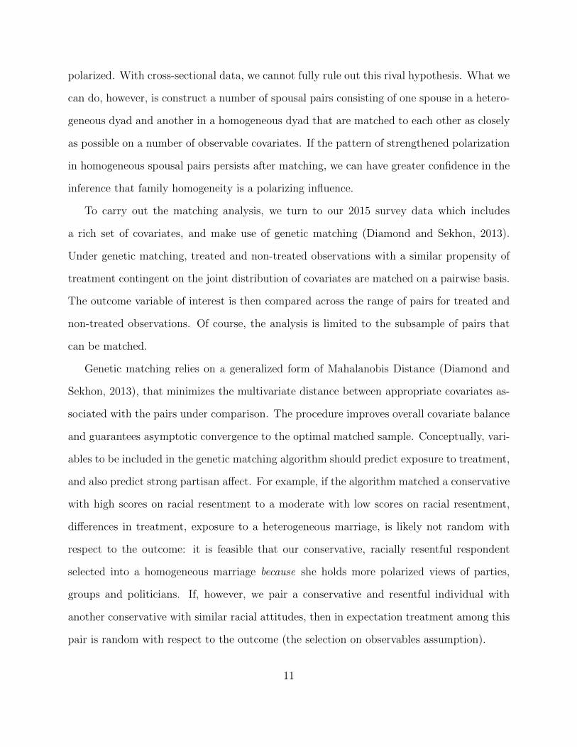
We begin by comparing the net in- and out-party ratings across homogeneous and hetero-

geneous spousal pairs, noting that the party feeling thermometers represent the most direct

indicator of partisan affect. Because the 1965 socialization survey lacked thermometers tar-

geting parties, our analysis here is restricted to the 1997 wave of the youth-parent survey,

our 2015 survey, and the 2016 field experiments.

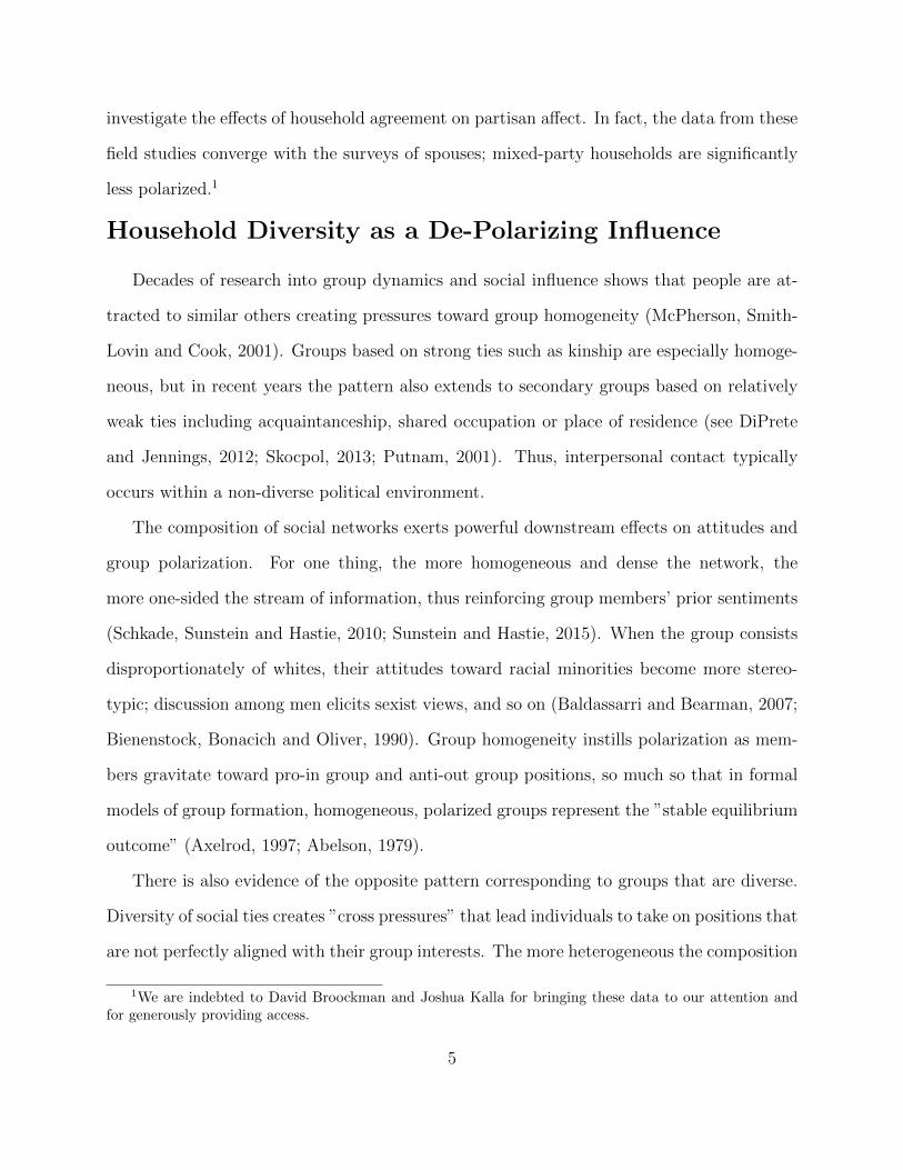
Aggregating across both sets of dyads, polarization increased substantially between 1997

and 2015. However, as shown in Figure 1, almost all the increase occurred among members

of homogeneous spousal dyads. For this group, the net party rating more than doubled

between 1997 and 2015. Individuals in heterogeneous dyads, although more polarized in

2015 than in 1997, underwent only modest movement.

Next, we turn to the question of whether increased polarization over time is attributable

to increased in-group favoritism or heightened hostility toward the out group. In Figure 1,

we show the separate thermometer ratings for the in and out party, respectively. It is clear

that increased polarization stems primarily from downward movement in the thermometer

rating of the out party. The mean drops from 41.73 in 1997 to 17.96 in 2015 for spouses

in politically homogeneous marriages, and – to a lesser extent – from 46.27 to 31.27 for

spouses in heterogeneous marriages. Consistent with the longitudinal data on the question

(see Iyengar, Sood and Lelkes, 2012), partisans’ favorable ratings of fellow partisans have

remained generally stable between 1997 and 2015. The steep decline in the ratings of the

out party is concentrated among individuals in homogeneous households. Quite strikingly,

the 1997-2016 difference in the out party thermometer score is not significant for individuals

in heterogeneous spousal pairs.

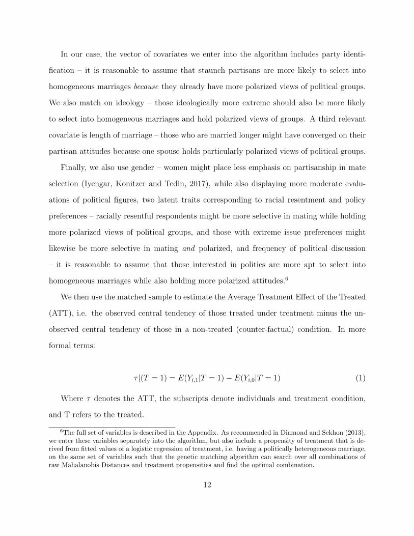
We turn next to polarization in ratings of presidential candidates. As in the case of the

13

0

20

40

60

1997 2015 2016

Diff

eren

ce In

part

y−O

utpa

rty

Type

Homogeneous

Non−Homogeneous

0

20

40

60

80

1997 2015 2016

Inpa

rty

Type

Homogeneous

Non−Homogeneous

0

10

20

30

40

50

1997 2015 2016

Out

part

y

Type

Homogeneous

Non−Homogeneous

Figure 1: Net (In-Out) Party (upper panel), In-Party (bottom left Panel) and Out-Party(bottom right panel) Ratings for Homogeneous and Heterogeneous Spousal Pairs

14

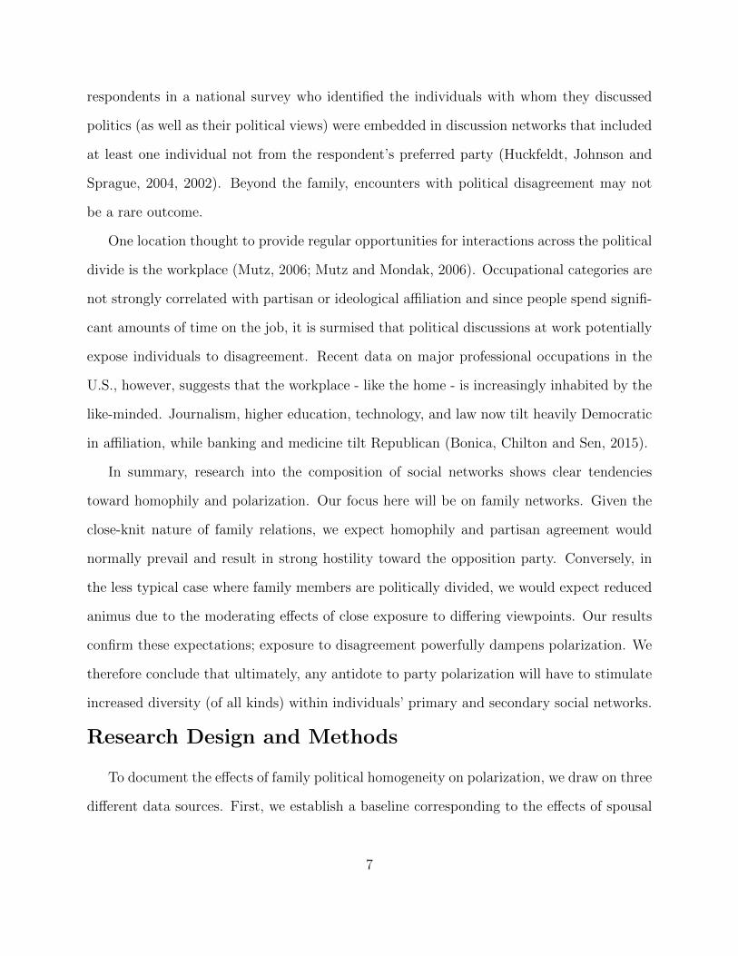
party ratings, polarized evaluations of the candidates rose substantially post-1997 among

individuals in both homogeneous and heterogeneous dyads (see Figure 2).7 While the gap

in affective polarization, i.e. the difference between the in- and out-candidate rating, across

homogeneous and non-homogeneous pairs was sizable even in 1997 (6.68 points), it jumped

dramatically in 2015 to 26.3 points, with a similar gain in 2016 registered among respondents

in the field experiments (20.34 points).

Once again, we can address the question of whether increased polarization reflects move-

ment in favoritism for the in group, or hostility toward the out group. As shown in Figure 2,

increased polarization stems primarily from downward movement in the thermometer rating

of the out candidate. The mean drops precipitously from 36.89 in 1997 to 9.52 in 2015

for spouses in politically homogeneous marriages. In the case of spouses in heterogeneous

marriages, the fall in the out-party rating is not as massive, from 43.66 to 21.96. Replicating

the pattern of the party ratings, partisans’ favorable ratings of the in candidate remained

generally stable between 1997 and 2016.

7Note that we have no appropriate candidate-related measures from the 1965 wave of the socializationstudy.

15

0

20

40

60

1997 2015 2016Del

ta In

cand

idat

e−O

utca

ndid

ate

Type

Homogeneous

Non−Homogeneous

0

20

40

60

1997 2015 2016

Inca

ndid

ate

Type

Homogeneous

Non−Homogeneous

0

10

20

30

40

1997 2015 2016

Out

cand

idat

e Type

Homogeneous

Non−Homogeneous

Figure 2: Net (In-Out) Candidate (upper panel), In-Candidate (bottom left Panel) andOut-Candidate (bottom right panel) Ratings for Homogeneous and Heterogeneous SpousalPairs

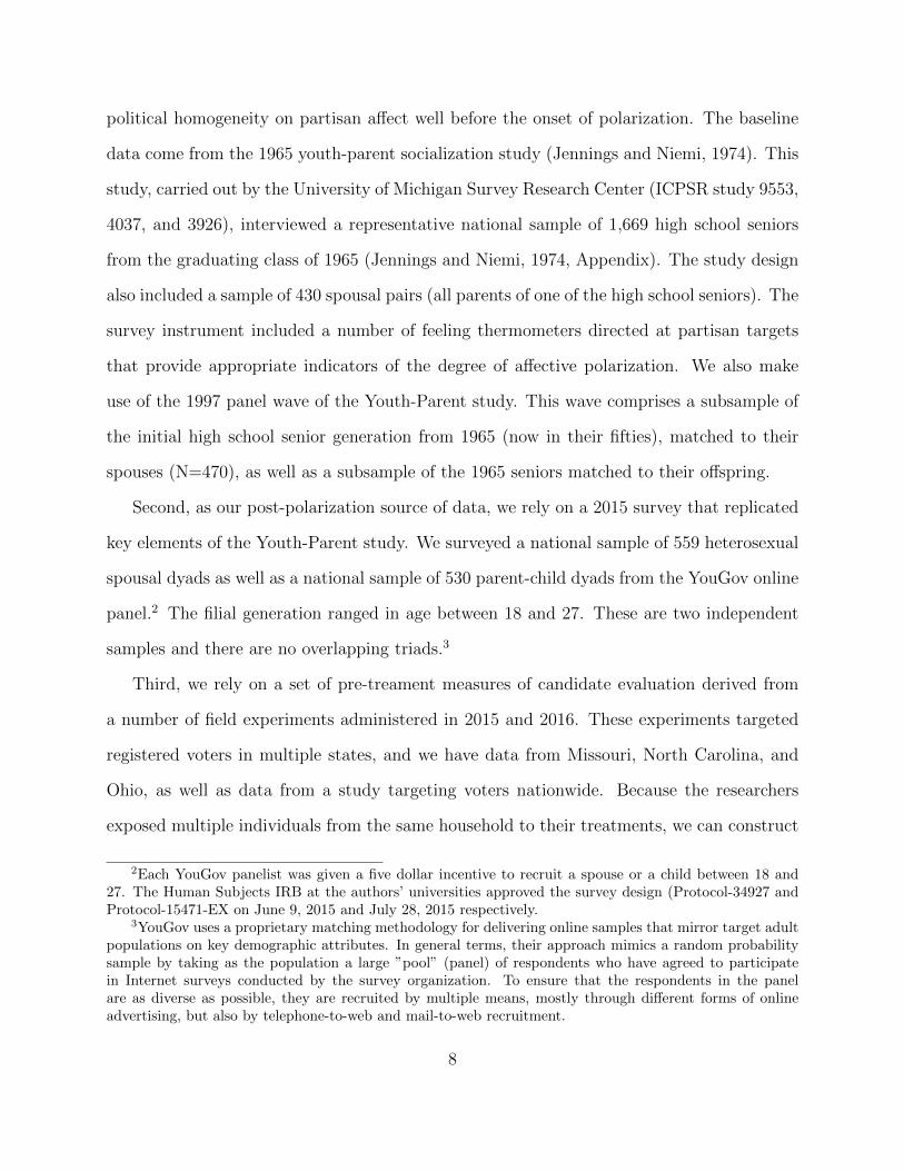
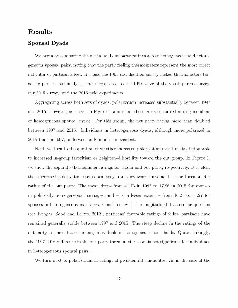
As our third indicator of partisan affect, we turn to evaluations of groups loosely affiliated

with the parties. As shown in Figure 3, polarized evaluations of partisan groups increased

post-1997 among individuals in both homogeneous and heterogeneous dyads. The relevant

difference-in-difference moves from -0.36 (i.e. virtually no difference between homogeneous

and heterogeneous pairs) to 6.29 points in 1997, before peaking at 16.84 points in 2015.

As with the party and candidate ratings, the increased polarization over time is far more

pronounced among individuals in homogeneous spousal pairs. These individuals underwent

a steady increase in polarization between 1965 and 1997, and 1997 and 2015. For individuals

in mixed pairs, there is no change at all between 1965 and 1997, and only modest change

thereafter.

The group evaluations further confirm that the trend in polarization occurs because of

16

changes in out group animus rather than in group favoritism. It is hostility toward the out

group that also accounts for the difference in the temporal pattern between homogeneous

and heterogeneous spousal pairs. Among individuals exposed to diversity in the home, the

rating of the out group shows only modest change between 1965 and 1997, and no change

between 1997 and 2015.

0

10

20

30

1965 1997 2015

Diff

eren

ce In

grou

p−O

utgr

oup

Type

Homogeneous

Non−Homogeneous

0

20

40

60

1965 1997 2015

Ingr

oup

Type

Homogeneous

Non−Homogeneous

0

20

40

60

1965 1997 2015

Out

grou

p

Type

Homogeneous

Non−Homogeneous

Figure 3: Net (In-Out) Group (upper Panel), In-Group (bottom left Panel) and Out-Group(bottom right panel) Ratings for Homogeneous and Heterogeneous Spousal Pairs

Our final analysis of spousal agreement focuses on Latino Republicans in the state of

Florida. As we noted at the outset, this group provides an especially strong test of the

network homogeneity hypothesis because they were subject to strong cross pressures once

their party nominated Donald Trump, whose inflammatory rhetoric on immigration was

widely interpreted as anti-Latino. We therefore expect less than enthusiastic support for the

in-party candidate among Latinos, thus dampening the potential effects of family networks

on polarization.

17

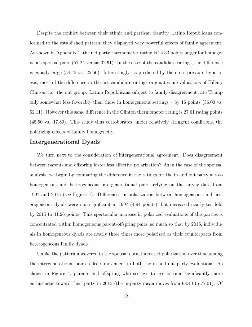
Despite the conflict between their ethnic and partisan identity, Latino Republicans con-

formed to the established pattern; they displayed very powerful effects of family agreement.

As shown in Appendix 1, the net party thermometer rating is 24.33 points larger for homoge-

neous spousal pairs (57.24 versus 32.91). In the case of the candidate ratings, the difference

is equally large (54.45 vs. 25.56). Interestingly, as predicted by the cross pressure hypoth-

esis, most of the difference in the net candidate ratings originates in evaluations of Hillary

Clinton, i.e. the out group. Latino Republicans subject to family disagreement rate Trump

only somewhat less favorably than those in homogeneous settings – by 16 points (36.00 vs.

52.11). However this same difference in the Clinton thermometer rating is 27.61 rating points

(45.50 vs. 17.89). This study thus corroborates, under relatively stringent conditions, the

polarizing effects of family homogeneity.

Intergenerational Dyads

We turn next to the consideration of intergenerational agreement. Does disagreement

between parents and offspring foster less affective polarization? As in the case of the spousal

analysis, we begin by comparing the difference in the ratings for the in and out party across

homogeneous and heterogeneous intergenerational pairs, relying on the survey data from

1997 and 2015 (see Figure 4). Differences in polarization between homogeneous and het-

erogeneous dyads were non-significant in 1997 (4.94 points), but increased nearly ten fold

by 2015 to 41.26 points. This spectacular increase in polarized evaluations of the parties is

concentrated within homogeneous parent-offspring pairs, so much so that by 2015, individu-

als in homogeneous dyads are nearly three times more polarized as their counterparts from

heterogeneous family dyads.

Unlike the pattern uncovered in the spousal data, increased polarization over time among

the intergenerational pairs reflects movement in both the in and out party evaluations. As

shown in Figure 4, parents and offspring who see eye to eye become significantly more

enthusiastic toward their party in 2015 (the in-party mean moves from 68.40 to 77.01). Of

18

course, these individuals also display the now familiar pattern of increased hostility toward

the out party; the mean thermometer score for the out party drops sharply from 45.03 in

1997 to 22.84 in 2015.

0

20

40

60

1997 2015

Del

ta In

part

y−O

utpa

rty

Type

Homogeneous

Non−Homogeneous

0

20

40

60

80

1997 2015

Inpa

rty

Type

Homogeneous

Non−Homogeneous

0

10

20

30

40

50

1997 2015

Out

part

y

Type

Homogeneous

Non−Homogeneous

Figure 4: Net Party (in-Out) (upper Panel), In-Party (bottom left panel) and Out-Party(bottom right panel) Rating for Homogeneous and Heterogeneous Intergenerational Pairs

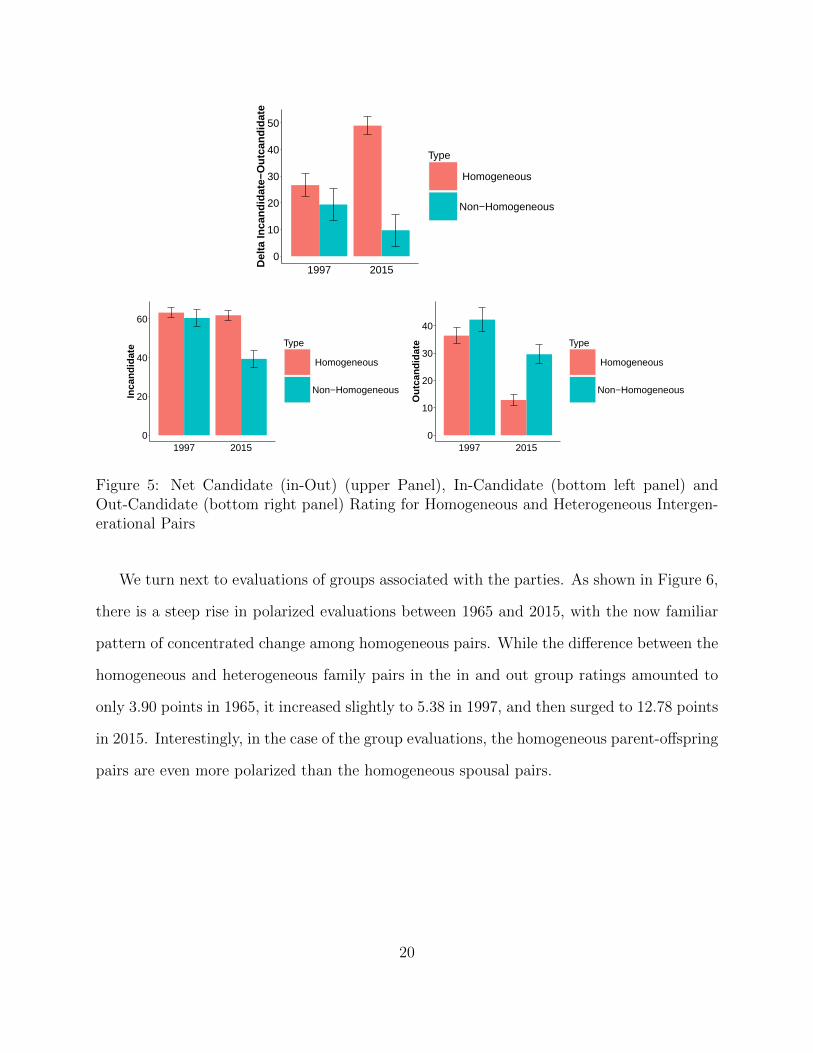
Turning to the candidate evaluations, similar dynamics emerge, as shown in Figure 5.

There was a negligible difference in polarization between homogeneous and heterogeneous

dyads in 1997. By 2015, however, the difference is pronounced, moving from 7.28 points to

39.24 points. Almost all the increase in the net candidate ratings is due to more unfavorable

evaluations of the opposing candidate. Increased hostility toward the opposition is, once

again, far more intense when parents and offspring agree.

19

0

10

20

30

40

50

1997 2015Del

ta In

cand

idat

e−O

utca

ndid

ate

Type

Homogeneous

Non−Homogeneous

0

20

40

60

1997 2015

Inca

ndid

ate

Type

Homogeneous

Non−Homogeneous

0

10

20

30

40

1997 2015

Out

cand

idat

e Type

Homogeneous

Non−Homogeneous

Figure 5: Net Candidate (in-Out) (upper Panel), In-Candidate (bottom left panel) andOut-Candidate (bottom right panel) Rating for Homogeneous and Heterogeneous Intergen-erational Pairs

We turn next to evaluations of groups associated with the parties. As shown in Figure 6,

there is a steep rise in polarized evaluations between 1965 and 2015, with the now familiar

pattern of concentrated change among homogeneous pairs. While the difference between the

homogeneous and heterogeneous family pairs in the in and out group ratings amounted to

only 3.90 points in 1965, it increased slightly to 5.38 in 1997, and then surged to 12.78 points

in 2015. Interestingly, in the case of the group evaluations, the homogeneous parent-offspring

pairs are even more polarized than the homogeneous spousal pairs.

20

0

10

20

1965 1997 2015D

iffer

ence

Ingr

oup−

Out

grou

p

Type

Homogeneous

Non−Homogeneous

0

20

40

60

1965 1997 2015

Ingr

oup

Type

Homogeneous

Non−Homogeneous

0

20

40

60

1965 1997 2015

Out

grou

p

Type

Homogeneous

Non−Homogeneous

Figure 6: Net Group (in-Out) (upper Panel), In-Group (bottom left panel) and Out-Group(bottom right panel) Rating for Homogeneous and Heterogeneous Intergenerational Pairs

Selection Effects

Despite the remarkable stability of our results, and the successful replication across mul-

tiple data sets, the finding of greater polarization within homogeneous families may reflect

not the moderating influences of network diversity, but a selection bias instead. Individuals

with more polarized attitudes may be attracted to mates whose views are compatible. In

an attempt to neutralize possible selection effects, we use genetic matching and compute

the Average Treatment Effect among the Treated (ATT), i.e. the estimated causal effect of

heterogeneous marriage on our outcomes of interest8

8Balance statistics are included in the Appendix.

21

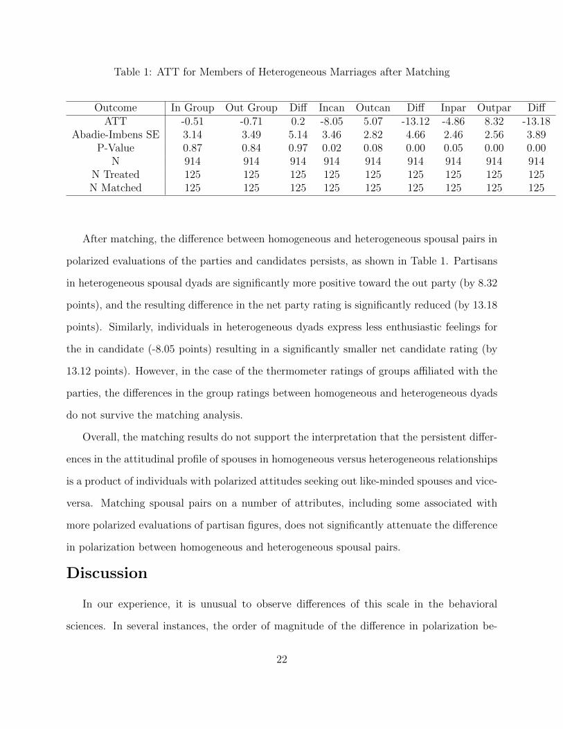
Table 1: ATT for Members of Heterogeneous Marriages after Matching

Outcome In Group Out Group Diff Incan Outcan Diff Inpar Outpar DiffATT -0.51 -0.71 0.2 -8.05 5.07 -13.12 -4.86 8.32 -13.18

Abadie-Imbens SE 3.14 3.49 5.14 3.46 2.82 4.66 2.46 2.56 3.89P-Value 0.87 0.84 0.97 0.02 0.08 0.00 0.05 0.00 0.00

N 914 914 914 914 914 914 914 914 914N Treated 125 125 125 125 125 125 125 125 125N Matched 125 125 125 125 125 125 125 125 125

After matching, the difference between homogeneous and heterogeneous spousal pairs in

polarized evaluations of the parties and candidates persists, as shown in Table 1. Partisans

in heterogeneous spousal dyads are significantly more positive toward the out party (by 8.32

points), and the resulting difference in the net party rating is significantly reduced (by 13.18

points). Similarly, individuals in heterogeneous dyads express less enthusiastic feelings for

the in candidate (-8.05 points) resulting in a significantly smaller net candidate rating (by

13.12 points). However, in the case of the thermometer ratings of groups affiliated with the

parties, the differences in the group ratings between homogeneous and heterogeneous dyads

do not survive the matching analysis.

Overall, the matching results do not support the interpretation that the persistent differ-

ences in the attitudinal profile of spouses in homogeneous versus heterogeneous relationships

is a product of individuals with polarized attitudes seeking out like-minded spouses and vice-

versa. Matching spousal pairs on a number of attributes, including some associated with

more polarized evaluations of partisan figures, does not significantly attenuate the difference

in polarization between homogeneous and heterogeneous spousal pairs.

Discussion

In our experience, it is unusual to observe differences of this scale in the behavioral

sciences. In several instances, the order of magnitude of the difference in polarization be-

22

tween similar and dissimilar family pairs exceeded 200 percent! Even more unusual is the

fact that our results survived multiple replications spanning different research designs, elec-

toral contexts, and survey indicators of partisan affect. While we acknowledge the causal

threat posed by selection effects, i.e. potential spouses with polarized attitudes selecting

into homogeneous marriages, the matching analysis does little to bolster this alternative

explanation.9 In total, the story line is unmistakable; political disagreement within family

relations discourages extreme evaluations of in and out groups, thus alleviating polarization.

Of course, documenting the powerful effects of family diversity on partisan affect begs

the question of what exactly is the mechanism through which exposure to disagreement

moderates individuals’ evaluations of the parties. One possibility is that domestic tranquility

requires the expression of opinions that respect the positions of significant others, making

individuals more tolerant and accepting of disagreement. Alternatively, as suggested by the

classic “contact” hypothesis (Allport, 1954; Pettigrew, 1998, 1997), valued inter-personal

relations that cut across the party divide may serve to weaken negative stereotypes of the

out group; for contrary evidence, however, see Enos (2014). Yet another possible mechanism,

also suggested by previous research (Mutz, 2006), is that inter-personal contact heightens

awareness of the values and arguments underlying the preferences of out party supporters,

making the party appear less threatening. All these mediating mechanisms appear to be

contingent on exposure to the opponent’s point of view; we would anticipate, accordingly,

that the effects of family diversity on partisan evaluations will be enlarged when family

members frequently converse about public affairs.

While our results imply that cross-party family ties are a potential antidote to polariza-

tion, it is important to keep in mind that this ”treatment” only impacts a relatively small

swath of American partisans. The most recent data on inter-marriage indicate that less

9Although while matching might tackle the selection problem more appropriately then parametric re-gression analyses, we note that the identification assumption remains selection-on-observables.

23

than twenty percent of partisans are exposed to disagreement. The likelihood that parti-

sans’ children will diverge on political grounds is similarly remote; in a 2015 survey, 74.2

percent of parent-offspring dyads agreed on their partisan affiliation (Iyengar, Konitzer and

Tedin, 2017). The critical question, therefore, concerns the ways in which society can lower

the barriers to social exchange across the party divide.

In theory, one solution to the problem of politically homogeneous networks is to weaken

individuals’ ability to signal their political affiliation. If all participants in the marriage

or dating market were ”blind” to partisan affiliation, partner selection would be driven

primarily by non-political attributes. Rational ”sellers” should deliberately conceal their

political views when seeking out potential mates. In fact, the evidence from online dating

sites suggests that most users of these sites behave strategically: they choose to remain

silent about their political attitudes. Research into the content of online daters’ personal

profiles shows that less than fifteen percent of online daters provided information about

their “political interests” and when they did reference politics in their personal profile, they

identified themselves as “middle of the road”(Klofstad, McDermott and Hatemi, 2012). This

same study shows, revealingly, that online daters are more willing to divulge their weight

than their political preferences.

Online databases provide opportunities for people to sort into relationships on the basis

of attributes extraneous to partisanship. Since some twenty percent of single individuals

report using online dating sites, technology might be a tool for dampening polarization.

Yet, as Huber and Malhotra (2017) have recently demonstrated, individuals manage to

unearth information about their prospective partner’s political views despite the lack of

transparency; so much so, that political ideology is the strongest predictor of successful

online match making. The motivation to find a politically compatible mate is sufficient to

overcome online daters’ lack of transparency about their politics.

In closing, our results show that partisan attitudes are distinctly less polarized when close

24

inter-personal ties are not based on the criterion of political similarity. For those seeking

to reduce animus and conflict across party lines, it is important to design meeting places

or platforms on which people become less focused on questions of political identity as an

important basis for their inter-personal relations.

25

References

Abelson, Robert P. 1979. “Social clusters and opinion clusters.” Perspectives in social net-

work research pp. 239–256.

Abramowitz, Alan. 2010. The disappearing center: Engaged citizens, polarization, and Amer-

ican democracy. Yale University Press.

Allport, Gordon W. 1954. The nature of prejudice. Basic books.

Asch, Solomon E and H Guetzkow. 1951. “Effects of group pressure upon the modification

and distortion of judgments.” Groups, leadership, and men pp. 222–236.

Axelrod, Robert. 1997. “The dissemination of culture: A model with local convergence and

global polarization.” Journal of conflict resolution 41(2):203–226.

Baldassarri, Delia and Peter Bearman. 2007. “Dynamics of political polarization.” American

sociological review 72(5):784–811.

Bienenstock, Elisa Jayne, Phillip Bonacich and Melvin Oliver. 1990. “The effect of network

density and homogeneity on attitude polarization.” Social Networks 12(2):153–172.

Bogardus, Emory S. 1925. “Social Distance and Its Origins.” Journal of Applied Sociology

9:216–226.

Bonica, Adam, Adam S Chilton and Maya Sen. 2015. “The Political Ideologies of American

Lawyers.” Journal of Legal Analysis 8(2):277–335.

Brown, Rupert and Miles Hewstone. 2005. “An integrative theory of intergroup contact.”

Advances in experimental social psychology 37:255–343.

26

Chen, Jowei and David Cottrell. 2016. “Evaluating partisan gains from Congressional ger-

rymandering: Using computer simulations to estimate the effect of gerrymandering in the

US House.” Electoral Studies 44:329–340.

Chen, Jowei, Jonathan Rodden et al. 2013. “Unintentional gerrymandering: Political geogra-

phy and electoral bias in legislatures.” Quarterly Journal of Political Science 8(3):239–269.

Diamond, Alexis and Jasjeet S Sekhon. 2013. “Genetic matching for estimating causal effects:

A general multivariate matching method for achieving balance in observational studies.”

Review of Economics and Statistics 95(3):932–945.

DiPrete, Thomas A and Jennifer L Jennings. 2012. “Social and behavioral skills and the

gender gap in early educational achievement.” Social Science Research 41(1):1–15.

Enos, Ryan D. 2014. “Causal effect of intergroup contact on exclusionary attitudes.” Pro-

ceedings of the National Academy of Sciences 111(10):3699–3704.

Fiorina, Morris P, Samuel J Abrams and Jeremy C Pope. 2005. “Culture war.” The myth of

a polarized America .

Huber, Gregory A and Neil Malhotra. 2017. “Political homophily in social relationships:

Evidence from online dating behavior.” The Journal of Politics 79(1):269–283.

Huckfeldt, Robert, Paul E Johnson and John Sprague. 2002. “Political environments, polit-

ical dynamics, and the survival of disagreement.” The Journal of Politics 64(1):1–21.

Huckfeldt, Robert, Paul E Johnson and John Sprague. 2004. Political disagreement: The

survival of diverse opinions within communication networks. Cambridge University Press.

Iyengar, Shanto, Gaurav Sood and Yphtach Lelkes. 2012. “Affect, Not Ideology – A Social

Identity Perspective on Polarization.” Public opinion quarterly 76(3):405–431.

27

Iyengar, Shanto and Sean J Westwood. 2015. “Fear and loathing across party lines: New

evidence on group polarization.” American Journal of Political Science 59(3):690–707.

Iyengar, Shato, Tobias B. Konitzer and Kent Tedin. 2017. “The home as a political fortress:

Family agreement in an era of polarization.”.

Jennings, M Kent, Laura Stoker and Jake Bowers. 2009. “Politics across generations: Family

transmission reexamined.” The Journal of Politics 71(3):782–799.

Jennings, M Kent and Richard Niemi. 1974. “The political character of adolescents.” Prince-

ton, NJ .

Katz, Elihud and Paul Felix Lazarsfeld. 1955. Personal influence: the part played by people

in the flow of mass communications. Glencoe, Ill: Free Press.

Klofstad, Casey A, Rose McDermott and Peter K Hatemi. 2012. “Do bedroom eyes wear

political glasses? The role of politics in human mate attraction.” Evolution and Human

Behavior 33(2):100–108.

Lazarsfeld, Paul Felix, Bernard Berelson and Hazel Gaudet. 1948. “The peoples choice: how

the voter makes up his mind in a presidential campaign.”.

McPherson, Miller, Lynn Smith-Lovin and James M Cook. 2001. “Birds of a feather: Ho-

mophily in social networks.” Annual review of sociology 27(1):415–444.

Muste, Christopher P. 2014. “Reframing polarization: Social groups and culture wars.” PS:

Political Science & Politics 47(2):432–442.

Mutz, Diana C. 2002. “Cross-cutting social networks: Testing democratic theory in practice.”

American Political Science Review 96(1):111–126.

28

Mutz, Diana C. 2006. Hearing the other side: Deliberative versus participatory democracy.

Cambridge University Press.

Mutz, Diana C and Jeffery J Mondak. 2006. “The workplace as a context for cross-cutting

political discourse.” Journal of politics 68(1):140–155.

Pettigrew, Andrew M. 1990. “Longitudinal field research on change: Theory and practice.”

Organization science 1(3):267–292.

Pettigrew, Thomas F. 1997. “Generalized intergroup contact effects on prejudice.” Person-

ality and social psychology bulletin 23(2):173–185.

Pettigrew, Thomas F. 1998. “Intergroup contact theory.” Annual review of psychology

49(1):65–85.

Pettigrew, Thomas F and Linda R Tropp. 2000. “Does intergroup contact reduce prejudice?

Recent meta-analytic findings.” Reducing prejudice and discrimination 93:114.

Putnam, Robert D. 2001. Bowling alone: The collapse and revival of American community.

Simon and Schuster.

Rico, Guillem and M Kent Jennings. 2016. “The Formation of Left-Right Identification:

Pathways and Correlates of Parental Influence.” Political Psychology 37(2):237–252.

Schkade, David, Cass R Sunstein and Reid Hastie. 2010. “When deliberation produces

extremism.” Critical Review 22(2-3):227–252.

Sheagley, Geoffrey. forthcoming. “The effect of cross-cutting partisan debates on political

decision-making.” Party Politics .

Skocpol, Theda. 2013. Diminished democracy: From membership to management in Ameri-

can civic life. Vol. 8 University of Oklahoma press.

29

Sunstein, Cass R and Reid Hastie. 2015. Wiser: Getting beyond groupthink to make groups

smarter. Harvard Business Press.

Tajfel, Henri. 1970. “Experiments’in’intergroup’discrimination.” Scientific American 223:96–

102.

Tajfel, Henri and J. C. Turner. 1979. An integrative theory of intergroup conflict. Brooks/Cole

pp. 33–47.

Westwood, Sean J, Shanto Iyengar, Stefaan Walgrave, Rafael Leonisio, Luis Miller and Oliver

Strijbis. 2017. “The tie that divides: Cross-national evidence of the primacy of partyism.”

Unpublished paper .

30

Appendix 1: Raw Thermometer scores

Thermometer Dem – Dem Rep – Rep Dem – Rep Dem – Ind Rep – Ind Ind – Ind

1965Labor Unions 64.95 44.92 57.52 62.25 50.36 63.38

(N=388) (N=200) (N=94) (N=66) (N=54) (N=20)Big Business 62.13 62.96 61.87 61.70 70.70 71.26

(N=388) (N=200) (N=94) (N=66) (N=54) (N=20)1997

Democrats 70.25 39.56 55.61 56.60 44.43 51.43(N=287) (N=299) (N=163) (N=72) (N=61) (N=7)

Republicans 44.18 70.17 56.98 46.48 59.10 51.43(N=287) (N=299) (N=162) (N=71) (N=61) (N=7)

Bill Clinton 67.30 29.67 52.55 56.61 39.96 37.86(N=286) (N=299) (N=165) (N=72) (N=63) (N=7)

Bob Dole 44.51 66.67 55.86 45.49 53.80 52.86(N=284) (N=297) (N=163) (N=71) (N=62) (N=7)

Liberals 61.43 32.06 49.53 49.28 43.45 48.57(N=281) (N=296) (N=160) (N=69) (N=60) (N=7)

Conservatives 43.34 69.76 55.18 51.88 58.23 57.14(N=280) (N=299) (N=163) (N=69) (N=61) (N=7)

Labor Unions 59.72 38.44 48.48 54.96 43.69 57.5(N=279) (N=290) (N=159) (N=71) (N=58) (N=6)

Big Business 43.99 52.83 49.89 45.57 46.27 44.29(N=284) (N=293) (N=161) (N=70) (N=59) (N=7)

2015Democrats 80.46 18.10 57.03 56.11 24.69 32.08

(N=366) (N=490) (N=64) (N=56) (N=83) (N=62)Republicans 17.42 76.05 50.48 31.96 59.55 46.36

(N=366) (N=480) (N=64) (N=56) (N=83) (N=62)Hillary Clinton 79.11 6.95 46.94 54.5 13.25 29.10

(N=342) (N=493) (N=64) (N=56) (N=83) (N=62)Donald Trump 9.06 65.14 30.67 21.84 54.04 41.56

(N=341) (N=496) (N=64) (N=56) (N=83) (N=62)Atheists 57.29 29.22 45.38 41.05 30.23 31.98

(N=341) (N=496) (N=64) (N=56) (N=84) (N=60)Evangelical Christians 29.11 67.89 50.30 37.84 61.46 46.74

(N=342) (N=495) (N=64) (N=56) (N=82) (N=62)2016



Obama/Clinton 71.22 23.96 53.41 53.38 53.22 64.56(N=296) (N=163) (N=61) (N=111) (N=79) (N=32)

Trump 19.80 57.53 34.82 26.91 30.95 18.28(N=296) (N=163) (N=61) (N=111) (N=79) (N=32)

Table 2: Mean thermometer scores for Spousal Pairs with Varying Political Make Up

32

Thermometer Dem – Dem Rep – Rep Dem – Rep Dem – Ind Rep – Ind Ind – Ind

1965Labor Unions 65.50 51.17 62.16 62.12 56.42 57.33

(N=624) (N=502) (N=638) (N=186) (N=166) (N=62))Big Business 62.61 62.40 63.09 64.76 63.08 57.11

(N=624) (N=502) (N=638) (N=186) (N=166) (N=62))1997



Bill Clinton 68.59 33.89 52.47 53.94 39.6 52.56(N=96) (N=102) (N=101) (N=52) (N=50) (N=16)

Bob Dole 44.38 62.99 54.43 44.39 55.90 62.21(N=89) (N=101) (N=101) (N=49) (N=48) (N=14)

Liberals 61.89 41.12 53.43 52.40 46.24 46.07(N=91) (N=98) (N=98) (N=48) (N=45) (N=14)

Conservatives 45.49 70.08 58.08 45.74 60.37 53.00(N=90) (N=97) (N=98) (N=47) (N=43) (N=15)

Labor Unions 62.21 45.37 55.72 67.74 48.64 51.89(N=82) (N=89) (N=93) (N=46) (N=45) (N=16)

Big Business 47.89 52.91 48.86 43.94 51.88 45.33(N=85) (N=100) (N=99) (N=47) (N=48) (N=15)

2015Democrats 79.65 22.59 54.21 60.19 27.36 43.61

(N=380) (N=254) (N=108) (N=80) (N=58) (N=70)Republicans 23.09 74.38 48.55 31.71 62.33 42.90

(N=383) (N=253) (N=108) (N=78) (N=57) (N=70)Hillary Clinton 77.08 15.29 44.531 57.42 13.26 40.80

(N=384) (N=252) (N=108) (N=79) (N=58) (N=69)Donald Trump 17.78 58.04 40.81 28.48 53.71 33.59

(N=381) (N=254) (N=108) (N=79) (N=58) (N=70)Atheists 53.10 34.75 44.30 52.11 30.72 45.97

(N=382) (N=253) (N=108) (N=79) (N=58) (N=70)Evangelical Christians 36.80 66.02 50.66 40.70 55.55 44.61

(N=380) (N=254) (N=108) (N=79) (N=58) (N=70)

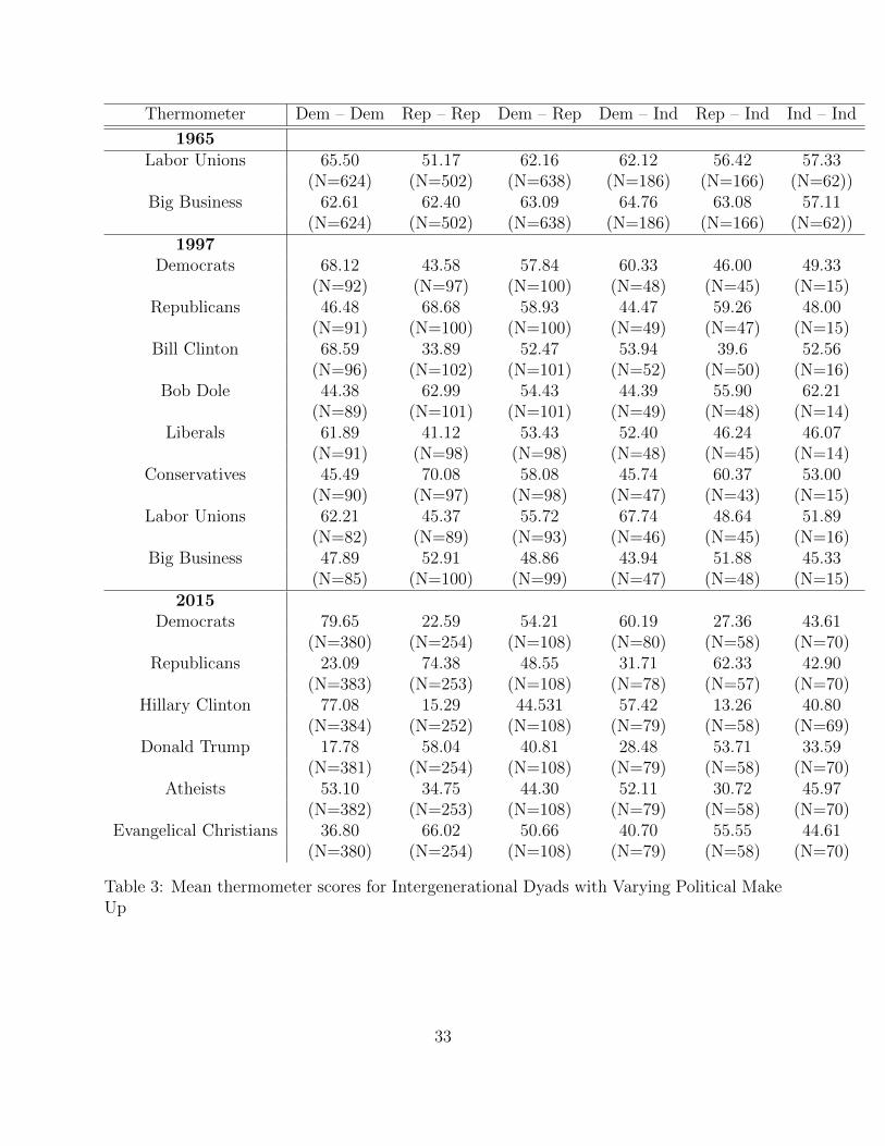
Table 3: Mean thermometer scores for Intergenerational Dyads with Varying Political MakeUp

33

Therm Ingrp Outgrp Diff Incan Outcan Diff Inpar Outpar Diff

ValidationHomogeneous NA NA NA 66.85 12.40 54.45 74.91 18.93 57.24Heterogeneous NA NA NA 45.35 19.79 25.56 52.63 28.33 32.91

1965Homogeneous 65.54 61.83 3.72 NA NA NA NA NA NAHeterogeneous 63.68 59.60 4.08 NA NA NA NA NA NA

1997Homogeneous 56.51 40.33 16.07 67.60 36.89 30.65 70.50 41.73 28.77Heterogeneous 53.62 44.11 9.78 62.29 43.66 18.54 64.68 46.27 18.30


2016Homogeneous NA NA NA 57.18 21.19 35.98 68.15 21.48 46.67Heterogeneous NA NA NA 44.89 29.56 15.64 55.45 37.40 18.05

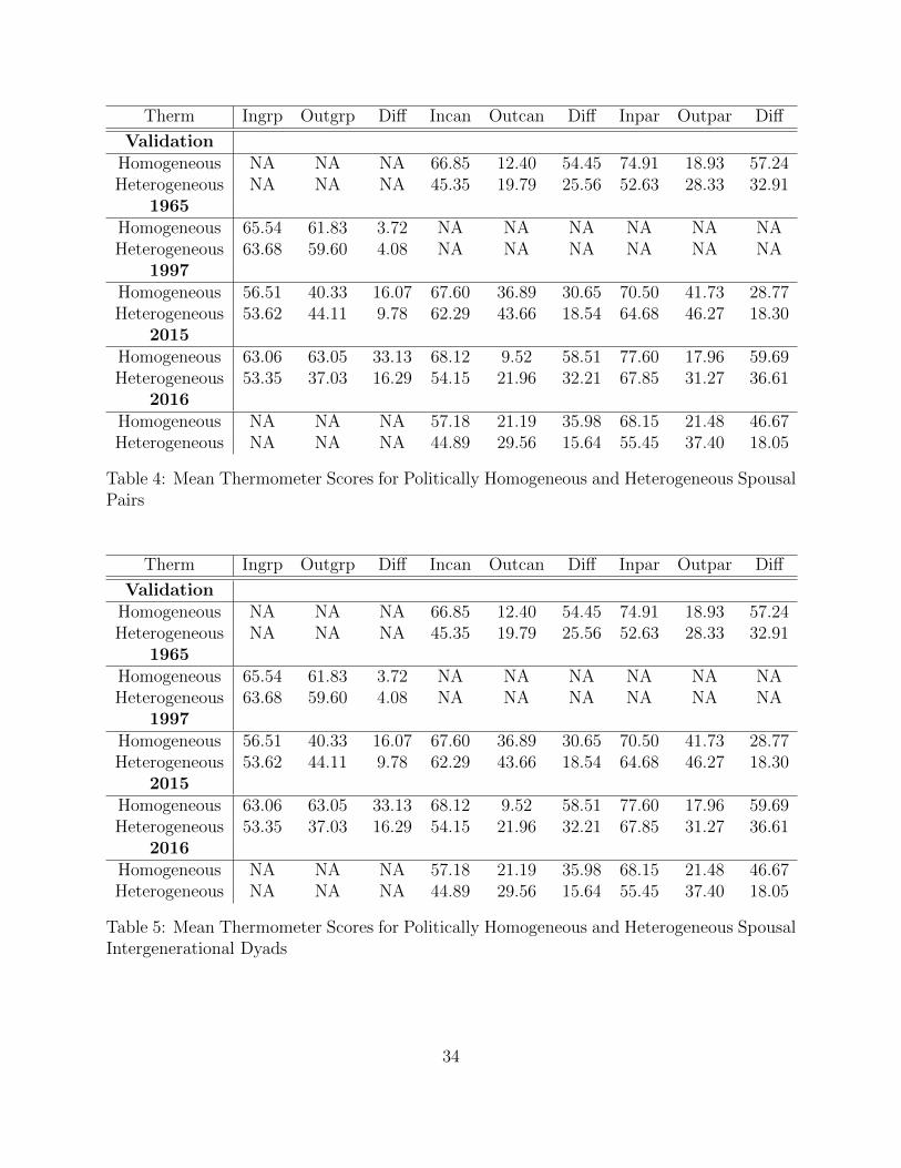
Table 4: Mean Thermometer Scores for Politically Homogeneous and Heterogeneous SpousalPairs

Therm Ingrp Outgrp Diff Incan Outcan Diff Inpar Outpar Diff

ValidationHomogeneous NA NA NA 66.85 12.40 54.45 74.91 18.93 57.24Heterogeneous NA NA NA 45.35 19.79 25.56 52.63 28.33 32.91

1965Homogeneous 65.54 61.83 3.72 NA NA NA NA NA NAHeterogeneous 63.68 59.60 4.08 NA NA NA NA NA NA



2016Homogeneous NA NA NA 57.18 21.19 35.98 68.15 21.48 46.67Heterogeneous NA NA NA 44.89 29.56 15.64 55.45 37.40 18.05

Table 5: Mean Thermometer Scores for Politically Homogeneous and Heterogeneous SpousalIntergenerational Dyads

34

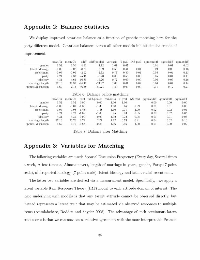
Appendix 2: Balance Statistics

We display improved covariate balance as a function of genetic matching here for the

party-differece model. Covariate balances across all other models inhibit similar trends of

improvement.

mean.Tr mean.Co sdiff sdiff.pooled var.ratio T pval KS pval qqmeandiff qqmeddiff qqmaxdiffgender 1.52 1.50 4.11 4.12 1.01 0.67 0.01 0.01 0.02

latent ideology -0.08 -0.02 -8.31 -7.39 0.65 0.41 0.01 0.09 0.09 0.16resentment -0.07 -0.05 -2.52 -2.32 0.73 0.80 0.04 0.05 0.04 0.13

party 4.21 4.33 -5.46 -5.20 0.83 0.58 0.06 0.05 0.04 0.11ideology 4.34 4.64 -16.89 -15.76 0.77 0.09 0.00 0.06 0.05 0.16

marriage length 27.16 31.35 -24.49 -24.97 1.08 0.01 0.02 0.06 0.07 0.14spousal discussion 1.69 2.13 -46.38 -50.74 1.49 0.00 0.00 0.11 0.12 0.21

Table 6: Balance before matchingmean.Tr mean.Co sdiff sdiff.pooled var.ratio T pval KS pval qqmeandiff qqmeddiff qqmaxdiff

gender 1.52 1.52 0.00 0.00 1.00 1.00 0.00 0.00 0.00latent ideology -0.08 -0.07 -1.30 -1.30 1.08 0.66 0.99 0.01 0.01 0.06

resentment -0.07 -0.08 1.48 1.48 1.10 0.71 1.00 0.02 0.02 0.05party 4.21 4.23 -1.08 -1.08 0.95 0.83 0.85 0.02 0.02 0.05

ideology 4.34 4.35 -0.90 -0.90 1.02 0.72 0.98 0.01 0.01 0.03marriage length 27.16 26.70 2.71 2.71 1.12 0.73 0.41 0.04 0.02 0.10

spousal discussion 1.69 1.70 -0.83 -0.83 1.06 0.56 1.00 0.01 0.00 0.02

Table 7: Balance after Matching

Appendix 3: Variables for Matching

The following variables are used: Spousal Discussion Frequency (Every day, Several times

a week, A few times a, Almost never), length of marriage in years, gender, Party (7-point

scale), self-reported ideology (7-point scale), latent ideology and latent racial resentment.

The latter two variables are derived via a measurement model. Specifically, , we apply a

latent variable Item Response Theory (IRT) model to each attitude domain of interest. The

logic underlying such models is that any target attitude cannot be observed directly, but

instead represents a latent trait that may be estimated via observed responses to multiple

items (Ansolabehere, Rodden and Snyder 2008). The advantage of such continuous latent

trait scores is that we can now assess relative agreement with the more interpretable Pearson

35

(r) correlation. The relevant test of increases in political homophily is change over time in

the strength of the spousal and intergenerational latent trait correlations.

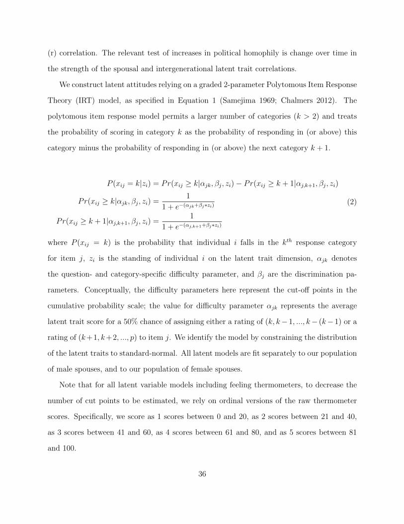
We construct latent attitudes relying on a graded 2-parameter Polytomous Item Response

Theory (IRT) model, as specified in Equation 1 (Samejima 1969; Chalmers 2012). The

polytomous item response model permits a larger number of categories (k > 2) and treats

the probability of scoring in category k as the probability of responding in (or above) this

category minus the probability of responding in (or above) the next category k + 1.

P (xij = k|zi) = Pr(xij ≥ k|αjk, βj, zi)− Pr(xij ≥ k + 1|αj,k+1, βj, zi)

Pr(xij ≥ k|αjk, βj, zi) =1

1 + e−(αjk+βj∗zi)

Pr(xij ≥ k + 1|αj,k+1, βj, zi) =1

1 + e−(αj,k+1+βj∗zi)

(2)

where P (xij = k) is the probability that individual i falls in the kth response category

for item j, zi is the standing of individual i on the latent trait dimension, αjk denotes

the question- and category-specific difficulty parameter, and βj are the discrimination pa-

rameters. Conceptually, the difficulty parameters here represent the cut-off points in the

cumulative probability scale; the value for difficulty parameter αjk represents the average

latent trait score for a 50% chance of assigning either a rating of (k, k− 1, ..., k− (k− 1) or a

rating of (k+1, k+2, ..., p) to item j. We identify the model by constraining the distribution

of the latent traits to standard-normal. All latent models are fit separately to our population

of male spouses, and to our population of female spouses.

Note that for all latent variable models including feeling thermometers, to decrease the

number of cut points to be estimated, we rely on ordinal versions of the raw thermometer

scores. Specifically, we score as 1 scores between 0 and 20, as 2 scores between 21 and 40,

as 3 scores between 41 and 60, as 4 scores between 61 and 80, and as 5 scores between 81

and 100.

36

Here, latent trait scores are calculated based on separate IRT models corresponding to

each of the domains of interest for which we have 1965 and 2015 data – partisan attitudes,

policy preferences, religious attitudes and personality – scaled separately for male and female

members of the marital pair. To assess relative agreement, we take the simple correlation

(r) between these continuous measures.

Variables Used:

Policy Preferences

Immigrants, ISIS/ground-troops, Death Penalty, Social Welfare, Income Inequality, Busi-

ness regulation, Services/Welfare, Health-Care, Abortion, Marijuana Legalization, Gay Mar-

riage

Policy Preferences Agree/Disagree - Racial minorities can overcame prejudice with-

out any special favors, Agree/Disagree - Racial minorities are not trying hard enough,

Agree/Disagree - Most racial minorities who receive welfare could get along without it if

they tried, Agree/Disagree - Generations of slavery and discrimination make it difficult for

Blacks to work their way out of the lower class

37

the moderating e ects of marriage across party lines · the moderating e ects of marriage across...

Documents