Scholars' Mine Scholars' Mine

Masters Theses Student Theses and Dissertations

Summer 2010

The mitigation effects of a barrier wall on blast wave pressures The mitigation effects of a barrier wall on blast wave pressures

Nathan Thomas Rouse

Follow this and additional works at: https://scholarsmine.mst.edu/masters_theses

Part of the Explosives Engineering Commons

Department: Department:

Recommended Citation Recommended Citation Rouse, Nathan Thomas, "The mitigation effects of a barrier wall on blast wave pressures" (2010). Masters Theses. 4998. https://scholarsmine.mst.edu/masters_theses/4998

This thesis is brought to you by Scholars' Mine, a service of the Missouri S&T Library and Learning Resources. This work is protected by U. S. Copyright Law. Unauthorized use including reproduction for redistribution requires the permission of the copyright holder. For more information, please contact scholarsmine@mst.edu.

THE MITIGATION EFFECTS OF A BARRIER WALL

ON BLAST WAVE PRESSURES

By

NATHAN THOMAS ROUSE

A THESIS

Presented to the Faculty of the Graduate School of the

MISSOURI UNIVERSITY OF SCIENCE AND TECHNOLOGY

In Partial Fulfillment of the Requirements for the Degree

MASTER OF SCIENCE IN EXPLOSIVES ENGINEERING

2010

Approved by:

Jason Baird, Advisor Paul N. Worsey

Kwame Awuah-Offei

iii

ABSTRACT

The study examined the mitigating effects of a blast barrier wall. This area of

blast mitigation is of interest due to the many different applications involved in protecting

a specific target from an explosive attack. The research follows a 1:50 scale layout using

73 gram, hemisphere-shaped, Composition-4 charges detonated at combinations of three

standoff distances from a blast barrier wall set at three different heights. This project

used 45 data points for each combination of standoff distance and wall height. This

project expanded prior research conducted by the United States Army Corps of Engineers

(USACE) by increasing the database of recorded pressures behind a barrier wall and

finding that a barrier wall creates an elongated effect on the pressure reduction area

behind the wall. In other words, the pressure reduction area extends more along the wall

than it does away from the wall.

The results of further study indicate how and to what extent the wall affects the

pressures created by the detonation of the Composition-4 hemispheres in the regions

selected. The distance at which the blast pressures were mitigated was affected by the

wall height and standoff distance. The wall height had a greater impact on the extent of

the percent pressure reduction than did the standoff distance; however, the standoff

distance has the greatest effect on the magnitude of the pressures behind a barrier wall.

In the end, it is hoped that the analysis contained in this thesis will aid in future

investigations of blast barrier walls and lead to more in-depth analyses and the creation of

more complex models to predict the effects of blast barrier walls on detonation shocks

and pressures from charges detonated at finite distances from the walls.

iv

ACKNOWLEDGEMENTS

I thank my advisors and professors in the Mining Engineering Department, Dr.

Jason Baird, Dr. Paul Worsey, and Dr. Kwame Awuah-Offei, for providing mentoring

and advice on explosives and data analysis for this project. In addition, the work of Phil

Mulligan was invaluable in obtaining and setting up the blast table at the beginning of

this project. I also thank Jim Taylor and DeWayne Phelps for their help and support at

the Experimental Mine.

I am grateful for the financial support I have received, and I particularly wish to

thank Barb Robertson and Shirley Hall for their help in obtaining this support.

Finally, I appreciate the support of my friends and family, and I thank The Grotto

for enabling me to make it through one more year of school.

v

TABLE OF CONTENTS

Page

ABSTRACT ....................................................................................................................... iii ACKNOWLEDGEMENTS ............................................................................................... iv

LIST OF ILLUSTRATIONS ............................................................................................ vii LIST OF TABLES ........................................................................................................... viii SECTION

1. INTRODUCTION ...................................................................................................... 1

2. REVIEW OF LITERATURE ..................................................................................... 5

3. EXPERIMENTAL PROCEDURE ........................................................................... 12

3.1. EQUIPMENT .................................................................................................... 12

3.1.1. Blast Table .................................................................................................. 13

3.1.2. Pressure Transducers .................................................................................. 17

3.1.3. Data Acquisition System............................................................................. 17

3.2. SETUP ............................................................................................................... 18

3.2.1. Blast Table .................................................................................................. 18

3.2.2. Pressure Transducers .................................................................................. 22

3.2.3. Data Acquisition System............................................................................. 24

3.3. TESTING PROCEDURE .................................................................................. 25

3.4. DATA RECOVERY AND MANIPULATION................................................. 27

4. RESULTS ................................................................................................................. 31

5. DISCUSSION ........................................................................................................... 36 5.1. STATISTICAL ANALYSIS ............................................................................. 36

5.2. PRESSURE VERSUS SCALED DISTANCE .................................................. 37

5.3. CONTOUR ANALYSIS ................................................................................... 39

5.4. GEOMETRIC AND SENSITIVITY ANALYSES ........................................... 46

5.5. EFFECT ON THE HUMAN BODY ................................................................. 49

5.6. CALIBRATION ANALYSIS ............................................................................ 51

6. CONCLUSIONS AND RECOMMENDATIONS ................................................... 53

6.1. CONCLUSION .................................................................................................. 53

6.2. FUTURE WORK AND RECOMMENDATIONS ........................................... 55

vi

APPENDIX ....................................................................................................................... 57

WORKS CITED ............................................................................................................... 63

VITA ................................................................................................................................. 64

vii

LIST OF ILLUSTRATIONS

Page

Figure 1.1. Blast table with charge and pressure recording locations ................................2

Figure 1.2. Test Scenario (Rickman and Murrell, 2004) ....................................................3

Figure 2.1. Blast wave diffraction over a barrier wall (Remennikov and Rose, 2007) .....................................................................7

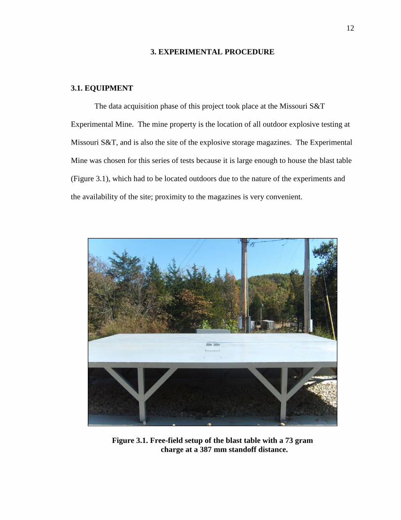
Figure 3.1. Free-field setup of the blast table with a 73 gram charge at a 387 mm standoff distance ........................................................12

Figure 3.2. Blast table depicting seven arcs of sample points ..........................................14

Figure 3.3. Plan view of the blast table with the three sample point layouts shown by different colors ..............................................................15

Figure 3.4. Blast table with dimensions and angles ..........................................................16

Figure 3.5. Synergy DAS ..................................................................................................18

Figure 3.6. Blast table with wall height of 73 mm............................................................19

Figure 3.7. Blast table with wall height of 226 mm..........................................................20

Figure 3.8. Charge setup (not to scale) .............................................................................21

Figure 3.9. Sample point locations and labels ..................................................................23

Figure 3.10. Screenshot of a free-field, 1219 mm standoff test data set ...........................28

Figure 4.1. Example of shadow area (387 mm standoff, 73 mm wall height) ..................33

Figure 4.2. Geometric relationship between the wall height, standoff distance, and location of the pressure reduction boundary ........................34

Figure 5.1. Combined standoff distance tests at wall heights of (a) 0 mm, (b) 73 mm, and (c) 226 mm ......................................................37

Figure 5.2. Percent reduction contour charts ....................................................................40

Figure 5.3. Relationship of alpha to beta at the shadow area boundary ...........................48

Figure 5.4. Sensitivity analysis of wall height and standoff distance ...............................49

Figure 5.5. Comparison of free-field data from USACE and Missouri S&T tests ....................................................................................52

viii

LIST OF TABLES

Page

Table 3.1. Comparison between steel and cardboard plates (The point column matches with sample point locations described in Figure 3.9) ..............................................................................................22

Table 3.2. Pressure transducer models and locations .......................................................23

Table 3.3. Pressure transducer calibration information ....................................................24

Table 3.4. Test matrix .......................................................................................................27

Table 3.5. Example of test results (387 mm standoff distance) ........................................30

Table 4.1. Free-field tests from Missouri S&T used in comparison with USACE tests...................................................................35

Table 5.1. Health Effects (Data from Zipf and Cashdollar, 2007 and Blast Effects Computer, 2001) ............................................................50

1

1. INTRODUCTION

Blast barrier walls can be used to mitigate explosive damage to target structures

that would otherwise be harmed by a blast from the detonation of an explosive charge.

Barrier walls serve two purposes in this instance:

1. They ensure that an explosive charge is set at a standoff distance away

from a protected object.

2. Up to a point, they diffract blast waves to mitigate the full force of the

blast pressures on the protected object.

This project is concentrated more with the latter purpose than the former;

however, both purposes are addressed by the analysis outlined by this report. It is an

investigation of the factors that affect the performance of a barrier wall against the effects

of air blast and provides empirical data and analysis that can facilitate the design of an

effective blast barrier wall. This analysis is important in that it will provide an idea for a

simple empirical model to aid in the design of a blast barrier wall and address multiple

ways the wall can aid in blast mitigation. The results will be useful to the U.S.

Department of State, the U.S. Department of Energy, the U.S. Department of Defense,

and civilian nuclear power stations that must protect facilities from vehicle bomb threats

or any other mobile explosive threat. Additionally, the data collected can be used to

help complete neural network software tools used in blast mitigation design and analysis.

For this research, various wall heights, explosive standoff distances, and data

point locations were used to record the pressures created by explosive charges. Pressure

transducers were located at various angles to an imaginary axis intersecting the charge

2

locations and the center point of the barrier wall (Figure 1.1). The transducers were

located on the opposite side of the wall from the charge positions at specified angles to

the axis. The data recorded by the pressure transducers were compared using charts and

graphs of the pressures, scaled distances, and data point locations.

Figure 1.1. Blast table with charge and pressure recording locations.

The tests conducted in this project explored the effects of a blast barrier wall on

an explosive pressure wave using experiments with a 1:50 scale setup. The scale up

3

simulates a 9,071 kg (20,000 lb) Composition-4 charge at standoff distances of 19.2 m,

61.0 m, and 102.4 m (63 ft, 200 ft, and 336 ft) and barrier wall heights of 3.7 m and 11.3

m (12 ft and 37 ft). This size of charge simulates a box truck or water/fuel truck bomb

scenario (Figure 1.2). The scaled setup included the charge size, barrier wall height, and

distances at which the pressures were recorded. The barrier wall tests were conducted on

a large steel blast table at the Missouri University of Science and Technology (Missouri

S&T) Experimental Mine. This blast table is similar to one at the United States Army

Corps of Engineers’ (USACE) Geotechnical and Structures Laboratory, which was used

by researchers to produce the report upon which this project builds (Rickman and

Murrell, 2004). That report offers three recommendations for future research. The

present work addressed each of the three:

Figure 1.2. Test Scenario (Rickman and Murrell, 2004).

4

analysis of the off-axis pressure locations, expansion of the database of recorded

pressures, and evaluation of the shielded area. It also analyzed the relationship between

the barrier wall height and standoff distance and the effect the two parameters had on the

area behind the barrier wall.

Primarily, this thesis does more than just expand on the research produced by the

USACE. Most importantly, the data was used to determine the extent of the area of

influence behind the barrier wall where the blast pressures are most affected by the wall.

This area was then studied to determine the individual factors that had the greatest effect.

Additionally, the health benefits of reducing the pressures were also reviewed since a

reduction in blast pressures at locations protected by barrier walls could equal a reduction

in fatality and/or injury rates.

5

2. REVIEW OF LITERATURE

For many years, structures have undergone blast loads due to large-scale blasts.

These large-scale blasts were caused by devices ranging from terrorist devices and

conventional explosive charges to nuclear weapons. For example, 5.5 tons of explosives

in a vehicle bomb were detonated at the U.S. Marine Corps Battalion Headquarters in

Beirut in 1983. Over 300 people were killed or wounded in the attack, which demolished

the concrete building in contact with the vehicle. In 1984, in Antilias, East Beirut, 2.8

tons of explosives were used to attack the U.S. Embassy Annex. In this case, the car

bomb was detonated on a sunken road approaching the Annex car park, and a small

retaining wall provided some shielding to the blast at a standoff distance from the

embassy. Due to the barrier wall, the casualty rate was relatively low and only 11 deaths

were recorded (Smith and Hetherington, 1994). These two contrasting scenarios give

some idea of how important blast barrier walls can be in situations involving explosive

attacks.

To understand how a blast pressure wave interacts with a barrier wall, one must

first understand a free-field blast pressure wave. The supersonic detonation within a high

explosive forms gases which undergo violent expansion. This expansion causes the

surrounding layer of air to compress and form a blast wave. The blast wave which

follows the detonation shock wave is a high pressure wavefront that expands out from the

explosive charge. It is followed by a negative pressure trough before the air resumes its

natural equilibrium at atmospheric pressure (Johansson and Persson, 1970 and Smith and

Hetherington, 1994).

6

For this project, the pressure wave is formed by a hemispherical charge on the

table surface. The shock front that the charge produces travels along the surface of

contact and expands outward from the charge into the atmosphere. In a free-field

application, this blast wave propagates along the surface until it is no longer supersonic.

It behaves this way until a structure, such as a barrier wall, is introduced. The barrier

wall in this project simulates a blast interaction with a large target. The blast wave from

a charge at some standoff distance impacts the barrier wall, which, due to its size and

construction does not move. This causes the blast wave to diffract over the barrier wall

(Figure 2.1). The wave is reduced for some distance behind the barrier wall before that

distance becomes large enough that the pressures are no longer affected by the wall

(Smith and Hetherington, 1994 and Remennikov and Rose, 2007). The area where the

wall affects the blast pressures and causes a pressure reduction is defined as the shadow

area. The extent of this shadow area defines the effectiveness of the barrier wall with

respect to pressure reduction. This is the effect of blast barrier walls that was

investigated by the research leading to this thesis.

The effect of barrier walls on blast pressures has been studied prior to this

investigation. The Army Corps of Engineers’ Geotechnical and Structures Laboratory

published a report on research conducted on a blast table using Composition-4 (C-4)

explosive charges, and various wall heights and standoff distances (Rickman and Murrell,

2004). It is from the USACE report that this study primarily draws for experimental

setup and procedure. The USACE investigated how the pressures produced by an

explosive charge were affected by a blast barrier wall and the effectiveness of the

ConWep program in predicting the pressure reduction caused by the barrier wall.

7

Figure 2.1. Blast wave diffraction over a barrier wall (Remennikov and Rose, 2007).

ConWep software is used to calculate blast effects of conventional weapons, and in the

case of the USACE report, it can effectively calculate blast pressures and pressure

reduction caused by a barrier wall. ACE also concluded that the maximum effect of the

barrier wall was produced at the smallest standoff distance and largest wall height.

The USACE report suggested that off-axis pressure locations be analyzed, that the

database of recorded pressures be expanded, and that the shielded area be evaluated.

These recommendations were evaluated and are included in this study.

ConWep, the conventional weapons effects software created and maintained by

the USACE Protective Design Center, was not used for this study; however, the USACE

suggests that it can be used to predict the peak pressures produced over a barrier wall.

ConWep is based on charts in Army Technical Manual (TM) 5-855-1, Fundamentals of

Protective Design for Conventional Weapons, which contains information on structural

response to conventional weapons. Another technical manual, TM 5-853-3, Security

8

Engineering Final Design, contains methods for calculating pressures and impulses

behind a barrier wall; however, the circulation of these technical manuals is restricted and

both have limited availability (Remennikov and Rose, 2007). The software that was

available for use was the Blast Effects Computer (BEC), which is a program developed

by the U.S. Department of Defense Explosives Safety Board to aid in predicting blast

pressures from explosive devices for magazine site and storage evaluations based on the

casing, composition, and size of the device, as well as the explosion site and the

atmospheric conditions. The macro-enabled Microsoft Excel © spreadsheets in the BEC

calculate the TNT equivalence, scaled distance, time of arrival, over-pressure, reflected

pressure, impulse, duration, window breakage probability, eardrum rupture probability,

and lethality probability due to lung damage (Blast Effects Computer, 2001). This

program was used in this project to predict the pressures produced by the 73 gram charge

and to successfully check that the 1:50 scale-up to a 20,000 lb charge would produce

similar pressures at the scaled-up distances.

Other than within the USACE, there have been many studies on effects of blast

pressures on structures. The work of Remennikov and Rose (2007) addresses the use of

empirical data and neural networks to predict the area of effect of a blast barrier wall on

structures behind a wall. It investigated how a blast wave is affected by a barrier wall

and examined the physical changes that a blast wave undergoes by using an artificial

neural network. The advantage of artificial neural networks is in their speed. Predicting

blast effects could take hours using computational fluid dynamics (CFD) programs;

however, artificial neural networks combine results from tests and from CFD model runs

into data sets, and only take minutes to complete an analysis. Through empirical data, the

9

Remennikov and Rose study shows that the use of neural networks is a feasible option to

predicting pressures behind a barrier wall.

Zhou and Hao (2006) also describe the blast loading of structures behind a barrier

wall. Their study introduced formulae based on empirical results of pressures on a rigid

wall behind a barrier to predict peak reflected pressure and impulse. These formulas can

be used together with TM-1300, Structures to Resist the Effects of Accidental Explosions,

to estimate the impulse and pressure on buildings behind a barrier wall. The majority of

studies based on barrier wall research, such as those described, determine pressures on

structures behind a blast wall; however, they do little to study the barrier wall’s effect on

a blast wave without the interference of structures or how blast waves are affected by a

barrier to cause loads on structures behind the barrier. A study of a barrier wall’s effect

on a blast wave would help to fully understand the area of pressure reduction due to a

barrier wall and how a barrier wall affects the blast pressure on the horizontal plane.

Walter (2004) describes the process of measuring air blasts and details how to

properly use a pressure transducer. The article depicts how an explosive waveform

progresses and shows the difference between incident pressure, free-field pressure, and

reflected pressure. It explains that incident pressure and free-field pressure are

synonymous and describe the pressure created by an expanding shock wave. When the

free-field wave reflects from a surface, it creates a reflected pressure wave. Two types of

pressure transducers are used to measure these waves. Side-on transducers are used to

measure free-field pressures without interfering with the flow behind the shock wave,

while reflected-pressure transducers (such as those used in this study) are used to

measure reflected pressures at normal incidence to a rigid surface. This type of

10

transducer must be mounted flush to that surface. Walter’s document was used to define

the pressures that were of interest to this thesis research and aid in selecting the proper

pressure transducers for the experiment.

Two methods of scaling were used in this study, scaled distance and charge

weight scaling. This thesis research used scaled distance in order to compare calculations

with the scaled distance in the USACE report. Smith and Hetherington (1994) and

Cooper (1996) provide the definition, identification, and use of scaled distance. Scaled

distance can be described by more than one formula; however, and the most used formula

is the Hopkinson-Cranz model. This model, described by Smith et. al. as the ratio of

distance to the charge over the third root of the charge weight, was used by the USACE

investigation. The second use of scaling, charge weight scaling, was used to calculate the

size of the corresponding full-scale explosive charge based on the charge from the 1:50

scale experiments. When scaling up the size of an explosive charge to gain the

equivalent scale-up of pressure, the charge mass must be scaled correctly (Cooper, 1996).

Mass is based on volume; therefore, scaling mass is based on scaling the volume of the

charge. Since volume scales proportionally with respect to the cube of the scaling factor,

charge mass is also proportional to the cube of the scaling factor (i.e., to calculate the

full-scale charge size, the 1:50 scale model must be multiplied by 503.).

One major importance of blast barrier walls is the reduction of casualty rates due

to the standoff distance and effects on blast pressure created by a barrier wall. Pressure

levels that relate to certain critical organ failures in people differ depending on the

documentation; therefore there is a wide variability in pressure levels cited and their

relation to the reaction of the human body. TM 1300 states that the eardrum damage

11

threshold is at 5 psi overpressure, the lung damage threshold is at 30 to 40 psi

overpressure, and the lethality threshold is at 100 to 120 psi overpressure. Near 100%

lethality occurs at 200 to 250 psi overpressure (TM 1300, 1990). Zipf, et al. agree with

the pressures that invoke eardrum rupture; however, they state that the lung damage

threshold is at 15 psi overpressure, and that the fatality threshold is at 35 to 45 psi

overpressure. They also state that nearly 100% lethality occurs at 55 to 65 psi

overpressure (Zipf, R and Cashdollar, K, 2007). The similarity between the lung damage

threshold of TM 1300 and fatality threshold of Zipf, et. al. may be that lung damage is a

significant enough injury to cause death due to gas release from agitated alveoli of the

lungs (TM 1300). One aspect of blast waves that has a great effect on tissue is the

impulse, which was not studied in this project. Impulse is the integral of the pressure

versus time curve; therefore it is a function of the pressure and the time over which the

pressure has an effect on an object. As impulse increases, the tolerance of tissue or

structures to pressure decreases. The longer tissue or structures is affected by a blast

wave, the pressure the tissue or structure can withstand decreases (Zipf and Cashdollar,

2007). This thesis uses the more conservative numbers of Zipf, et al. in its analysis of

blast effects on human tissue damage and fatality rate.

12

3. EXPERIMENTAL PROCEDURE

3.1. EQUIPMENT

The data acquisition phase of this project took place at the Missouri S&T

Experimental Mine. The mine property is the location of all outdoor explosive testing at

Missouri S&T, and is also the site of the explosive storage magazines. The Experimental

Mine was chosen for this series of tests because it is large enough to house the blast table

(Figure 3.1), which had to be located outdoors due to the nature of the experiments and

the availability of the site; proximity to the magazines is very convenient.

Figure 3.1. Free-field setup of the blast table with a 73 gram charge at a 387 mm standoff distance.

13

3.1.1. Blast Table. The 6 m by 4.9 m (20 ft by 16 ft) steel table comprised three

separate sections (Figure 3.1). One side of the table contained three ignition areas, one

for each of the three standoff locations of the explosive charges. The opposite side of the

table had 111 pre-constructed data acquisition points radiating from the center point of

the barrier wall to the edges of the table. The final section was the blast barrier wall,

which could be raised as high as 0.8 m (32 in) above the plane of the table.

The data collection points were positioned in radiating arcs from the center point of the

wall opposite the points of detonation (Figure 3.2). The table had seven expanding arcs

of data points at distances of 8.4 cm, 24.9 cm, 49.8 cm, 100.0 cm, and 175.1 cm (3.3 in,

9.8 in, 19.6 in, 39.4 in, and 68.9 in) from the wall. The seven rows of arcs, from

innermost to outermost, consisted of 15 points, 17 points, 19 points, 19 points, 19 points,

16 points, and 6 points. Due to restrictions on the size of the experiments, data

acquisition system limitations, and to keep the sample size, costs, and time within

manageable limits, only 45 sample points out of a total of 111 possible points were used.

Arc 1 consisted of one sample point, arc 2 consisted of seven sample points, arc 3

consisted of seven sample points, arc 4 consisted of nine sample points, arc 5 consisted of

nine sample points, arc 6 consisted of eight sample points, and arc 7 consisted of four

sample points. The data acquisition system records up to 16 channels of data at once;

therefore, three layouts of pressure transducers were enough to cover the 45 chosen

sample points.

14

Figure 3.2. Blast table depicting seven arcs of sample points.

Forty-five points were chosen instead of utilizing the full 48 available points that

could have been recorded by the data acquisition system to keep with the intent to use

every other sample point on the table. Also, the three extra channels were kept open in

the event that one of the channels on the data acquisition system ceased to work properly.

If one channel began to malfunction, only 45 possible samples could be recorded. This

strategy prevented the project from unwanted downtime due to unpreventable problems

with the data acquisition system, such as a software or hardware malfunction.

The sample points were chosen such that the final data would yield as much

information as possible on the pressures affected by the barrier wall while demanding the

15

fewest possible test iterations. The 45 sample points represented less than 50% of the

available data points; however, the sample point layout was designed to ensure that all

critical data was gathered by analyzing the entire table equally in all areas without

looking in-depth in any one region. If an in-depth analysis was required in any one

region, further testing could be completed to analyze that specific area.

Three standoff points were used in the blast table tests at distances of 387 mm,

1219 mm, and 2046 mm (15.25 in, 48 in, and 80.6 in) from the wall. The use of various

standoff distances was intended to indicate the extent to which a blast wave is affected by

the barrier wall when the charge was placed at different locations with respect to the wall

(Figure 3.3).

Figure 3.3. Plan view of the blast table with the three

sample point layouts shown by different colors.

16

The center point of each arc of transducer locations was on a line that passed

through the center of each blast location; that line was also perpendicular to the blast

wall. This line, which was deemed the 0 degree line, was used to identify the location of

data points at an angle to the axis (Figure 3.4). Therefore, the points were located by

degree of the angle to the axis (not by degree of the angle to the wall).

Figure 3.4. Blast table with dimensions and angles.

17

3.1.2. Pressure Transducers. Three models of high-resolution, PCB Integrated

Circuit-Piezoelectric pressure transducers (PCB Piezotronics, Inc, Depew, NY) were

utilized to determine the reflected pressure along the surface of the rigid table. An

important feature of the PCB transducers is they are integral-electronics piezoelectric

(IEPE) gages, which convert output from the transducer to a low impedance signal,

eliminating noise effects, and permitting the use of inexpensive cables that do not require

noise treatment. The pressure transducers were PCB Piezotronics Models 102B, 102B04,

and 102B15. Each transducer was calibrated for the expected pressure produced at its

location based on the results of the models in the Blast Effects Computer (Department of

Defense Explosives Safety Board, 2001). Model 102B can accurately measure pressures

ranging from 1 to 5000 psi; Model 102B04 can accurately measure pressures ranging

from 0.2 to 1000 psi; Model 102B15 can accurately measure pressures ranging from 0.05

to 200 psi.

3.1.3. Data Acquisition System. The Synergy Data Acquisition System (DAS)

(Hi-Techniques, Inc, Madison, WI) is a portable device incorporating signal conditioning,

a computer, memory, and a computer software package that was used in this project in its

oscilloscope mode to record the pressures created by each test (Figure 3.5). The DAS

can record up to 16 channels at once; thus, it dramatically reduced the number of tests

required by allowing 16 data points to be recorded for each shot. The important attribute

of this software/hardware package is that the Synergy DAS also has universal signal

conditioning incorporated into its software so that amplifiers were not required to boost

the signal from the pressure transducers to the DAS. Also, the data recorded during the

experiments could be saved to the hard drive for later analysis.

18

Figure 3.5. Synergy DAS 3.2. SETUP

Each test was set up using one of three layouts of pressure transducers, one of

three standoff distances, and one of three wall heights to keep the experimental setup

simple. The charge size and geometry were kept uniform. This was done to minimize

experimental error associated with any inconsistencies in the setup of the experiments.

Any variation in these factors could have potentially caused the pressures to behave

differently from one test to another.

3.2.1. Blast Table. The wall height of the blast table can be adjusted from 0 mm

(0 in) to 813 mm (32 in). Only three wall heights were chosen for this experiment: a

19

height of 0 mm was used for free-field tests to calibrate the table for comparison with

tests completed previously by the USACE (Rickman and Murrell, 2004) and to identify

the blast wave pattern without any obstruction. Barrier wall heights of 73 mm (2.9 in)

(Figure 3.6) and 226 mm (8.9 in) (Figure 3.7) were also chosen from among the six used

in the USACE tests. These wall heights were chosen from the USACE tests so that the

results could be compared between the two sites using identical wall heights, and the

chosen heights represent a broad view of the effects that the barrier wall height can have

on pressure reduction.

Figure 3.6. Blast table with wall height of 73 mm.

20

Figure 3.7. Blast table with wall height of 226 mm.

As noted in Section 3.1.1., three standoff distances were utilized in this project.

Each position consisted of a cut-out in the blast table, and a removable square steel plate.

The steel plates fit into the table cut-out, and a flange under the table around each cut-out

supported each plate. For each test in this experiment, the steel plate at the charge

location was replaced with a cardboard square to support the explosive charge, and each

square was drilled through the center with a ¼ in drill bit to create a location for

placement of a Dyno Nobel #1 MS Series Masterdet electric detonator (Figure 3.8).

21

Figure 3.8. Charge setup (not to scale).

The steel squares were replaced because they were more expensive than

cardboard squares and cost time to manufacture since they were useful for only a single

test. The cheap cardboard squares were easy to use as a replacement material for the

square plates. To examine the quality of the results when using a cardboard square, a test

was conducted using sample points along the axis and the free-field setup (Table 3.1).

During these tests, it was found that the steel plates spalled and damaged the

concrete foundation of the blast table. Also, as Table 3.1 shows, the difference in

pressures produced between tests using plates made of steel and cardboard is significant

enough to include an average adjustment. The average of the percent difference of steel

and cardboard for the five locations is 15%. The pressures produced using cardboard

plates on the blast table at Missouri S&T were increased by the 15% average to match

results that would be expected from using steel plates.

22

Table 3.1. Comparison between steel and cardboard plates (The point column matches with sample point locations described in Figure 3.9.)

3.2.2. Pressure Transducers. The pressure transducers were screwed into the

table from underneath until they were flush with the top of the blast table to minimize

disturbance in pressure readings. Then the transducers were connected to the Synergy

DAS by coaxial cables, which were inspected for any kinking that could have damaged

the cable or insulation or induced noise and disturbance in the pressure readings. Due to

the number of data points required for each combination of wall height and standoff

distance, testing was conducted using three separate transducer arrays. Table 3.2 and

Figure 3.9 match each transducer to its sample point location for each of the three arrays.

The points can be matched to the experimental results found in the Appendix. Figure 3.9

only shows the 45 sample points that were used in these tests; however, the labeling

convention includes all 111 points that are available for use on the table. The points were

labeled in this manner throughout the experiment because they weren’t physically

identified on the table. Keeping the layout uncomplicated like this was the easiest way to

ensure the correct sample points were used for every test.

PointPressures

using Steel (psi)

Pressures using

Cardboard (psi)

% Difference of Steel and Cardboard

8 118.690 105.371 11%24 59.848 57.174 4%42 37.365 27.659 26%61 15.943 13.224 17%80 6.611 5.491 17%

23

Table 3.2. Pressure transducer models and locations.

Figure 3.9. Sample point locations and labels.

Array 1 Array 2 Array 3102B 29322 18 8 28102B 29323 20 22 30102B 29324 35 24 45102B 29325 37 26 47102B 29327 39 49

102B04 29178 53 65102B04 29176 55 42 67102B04 29177 57 69102B04 29180 72 59 84102B04 29189 74 61 86102B04 29396 76 63 88102B15 29387 90 78 101102B15 29388 92 80 103102B15 29389 94 82 105102B15 29390 107 96 109

102B15 29395 108 99 110

Point relating to Figure 3.8

SerialModel

24

3.2.3. Data Acquisition System. The Synergy Data Acquisition System was

positioned under the transducer-side of the table behind a shield to minimize damage to

the computer while maintaining proximity to the transducers and thus eliminating the

need for an external signal amplifier. Table 3.3 summarizes the information provided by

PCB for each transducer, and used to calibrate the Synergy DAS. In addition to this

information, the DAS was set to capture the signal from each transducer as IEPE. The

Synergy DAS was set to recorder mode with a decimal timebase and sample rate of 5 µs

(200 kS/s). Recorder mode allows the oscilloscope files to be saved and loaded for

review at a later time, and the sample rate of 5 µs minimizes the file size while allowing

enough samples to be taken to record the pressure peaks accurately.

Table 3.3. Pressure transducer calibration information.

Model Number

Serial Number

Output Bias Level

(VDC)

Voltage Sensitivity (mV/psi)

Range (psi)

102B 29322 10.2 1.010 495102B 29323 10.2 1.009 496102B 29324 10.2 1.009 496102B 29325 10.2 1.018 492102B 29327 10.3 1.038 482

102B04 29178 10.2 5.032 199102B04 29176 10.1 4.993 200102B04 29177 10.1 4.989 200102B04 29180 10.0 5.038 198102B04 29189 10.1 5.014 199102B04 29396 10.2 5.063 198102B15 29387 9.0 24.88 80.4102B15 29388 10.1 24.47 81.7102B15 29389 10.1 25.33 79.0102B15 29390 10.1 24.71 80.9102B15 29395 10.0 24.82 80.6

25

3.3. TESTING PROCEDURE

Once the pressure transducers were in place and connected to the Synergry DAS,

testing was conducted according to the following procedure:

All cracks or gaps on the table were sealed with duct tape, the table was swept of

debris, and the gap between the two sides of the table was eliminated by clamping the

sides of the table together to minimize obstacles in the path of the blast wave and to

ensure repeatability. Then, C-4 was weighed into 73 (+/- 0.5) gram charges. Each

charge was pressed in a hollow, rubber mold to shape it into a hemisphere and then set on

the center of a cardboard square which had a ¼” hole drilled through its center. A Dyno

Nobel #1 MS Series Masterdet electric detonator was placed through the hole in the

cardboard and halfway into the 73 gram hemisphere of C-4. The mold kept the charge

from deforming while the detonator was inserted before the mold was removed. After

clearing the range of non-essential personnel, the charge assembly was placed on one of

the three charge locations, and the Synergy DAS was set to record the pressures from the

shot. The detonator lead-in lines were strung and connected to the blast cable, which was

shunted on the firing end. Finally, the blast cable was connected to an electric blasting

machine. The range was checked once more to ensure it was clear, and the charge was

detonated. The Synergy DAS was stopped, and the data was saved for later review.

To ensure the quality control of the experiments, each procedure was repeated according

to the above description. Because any variation in the setup could significantly affect the

results, the charges were placed in the same location at each standoff position and the

detonators were inserted the same depth in the charge for every shot. To remove any

potential disturbance from the table, all of the debris was cleared prior to each shot. The

26

wall height and pressure transducer array were not changed until each test requiring that

specific height and array was completed so there was no configuration difference in tests

of the same wall height or array. The test matrix (Table 3.4) shows that the tests for all

three standoffs were repeated for the first wall height and array. Then the array was

moved, keeping the wall height the same, and the nine tests for the three standoff

distances were completed again. This was repeated once more until all arrays and

standoff distances were tested for the first wall height. After the first 27 tests were

completed, the wall height was changed and the next set of 27 tests were completed.

Finally, the wall was set at its final height and the final 27 tests were conducted. All three

tests of each variable combination were completed on the same day to eliminate weather

as a factor in the results. In addition, all test sets were completed on days with similar

weather (partly cloudy, approximately 70°F, and little to no wind) at the elevation of

approximately 1150 ft above sea level. The Blast Effects Computer was used to

determine the actual effect that elevation and temperature has on the pressures created by

an explosive charge. An elevation change of 1,750 ft is required to change the pressure

of a blast by one psi. Also, temperature has an effect on the arrival time of the pressure

and not on the magnitude of the pressure. A change of 50° F is required to change the

arrival time by 1 ms (Blast Effects Computer, 2001). After this analysis, it is obvious

that the chance that weather has any effect on the results is relatively low compared to the

other factors mentioned throughout the report that may have caused variability in the

results. These other factors include the depth of placement of the detonator in the charge

because this could have caused variability in the data.

27

Table 3.4. Test matrix.

3.4. DATA RECOVERY AND MANIPULATION

Once testing was completed, each pressure recording (Figure 3.10) was

individually analyzed and the peak pressures recorded for each sample location. Figure

4.1 illustrates an example of one of the tests’ multiple pressure recordings (shot 6: 1219

Test Number Standoff (mm) Array Wall Height (mm)1, 2, 3 387 1 04, 5, 6 1219 1 07, 8, 9 2046 1 010, 11, 12 387 2 013, 14, 15 1219 2 016, 17, 18 2046 2 019, 20, 21 387 3 022, 23, 24 1219 3 025, 26, 27 2046 3 028, 29, 30 387 1 7331, 32, 33 1219 1 7334, 35, 36 2046 1 7337, 38, 39 387 2 7340, 41, 42 1219 2 7343, 44, 45 2046 2 7346, 47, 48 387 3 7349, 50, 51 1219 3 7352, 53, 54 2046 3 7355, 56, 57 387 1 22658, 59, 60 1219 1 22661, 62, 63 2046 1 22664, 65, 66 387 2 22667, 68, 69 1219 2 22670, 71, 72 2046 2 22673, 74, 75 387 3 22676, 77, 78 1219 3 22679, 80, 81 2046 3 226

28

mm standoff, 0 mm wall height, array 1) and shows the pressure wave for each of the 16

sample locations and the relative timing of the arrivals.

Figure 3.10. Screenshot of a free-field, 1219 mm standoff test data set.

For each combination of wall height, standoff distance, and transducer array, three

tests were completed for repeatability. Thus, there were 27 setup combinations and 81

tests. The results from each of the three tests of same wall height, standoff distance, and

transducer array were averaged at each individual data point location on the table to

create a “pressure set,” at each pressure recording point. The average of the three

29

pressures from each sample point was used to more accurately represent the performance

of the wall. The averaged results were recorded with the location of the data point and

the combination of variables used (Table 3.5 and Appendix). The data recorded from the

comparison test between the steel plate and cardboard plate gave a 15% difference

between the steel and the cardboard. Because of this, the data recorded when using the

cardboard plate had to be increased by 15% to account for the difference, as shown in the

Adjusted Pressure column in Table 3.5 and Appendix. Finally, the coordinate system for

the sample points sets the y-coordinate as the location along the length of the wall and the

x-coordinate as the distance away from the wall. The origin of the system is at the center

point of the wall and the axis running through the charge locations.

30

Table 3.5. Example of test results (387 mm standoff distance).

Point Y-Coordinates (mm) X-Coordinates (mm)Scaled Distance (m/(kg^(1/3)))

0 mm Wall Height, 387 mm Standoff Distance Pressure

(Pa)

73 mm Wall Height, 387 mm Standoff Distance Pressure

(Pa)

226 mm Wall Height, 387 mm

Standoff Distance Pressure (Pa)

8 0.0 84.1 2.42 726,508 55,158 26,216 18 230.2 96.8 7.19 580,612 124,106 25,138 20 174.6 177.8 7.17 475,948 137,895 29,195 22 96.8 231.8 7.23 454,190 151,685 30,654 24 0.0 249.2 7.18 394,199 165,474 32,392 26 -96.8 231.8 7.23 362,042 179,264 34,343 28 -174.6 177.8 7.17 497,043 193,053 32,396 30 -230.2 96.8 7.19 589,702 206,843 26,101 35 484.2 120.7 14.37 327,329 241,317 27,354 37 415.9 279.4 14.42 236,644 255,106 29,581 39 277.8 414.3 14.36 215,208 268,896 29,326 42 0.0 498.5 14.35 190,702 289,580 29,105 45 -277.8 414.3 14.36 219,377 310,264 30,585 47 -415.9 279.4 14.42 253,833 324,054 30,410 49 -484.2 120.7 14.37 353,455 337,843 26,384 53 992.2 103.2 28.72 129,569 365,422 24,099 55 927.1 382.6 28.87 104,945 379,212 28,712 57 708.0 706.4 28.79 86,529 393,001 24,532 59 385.8 925.5 28.87 78,812 406,791 22,806 61 0.0 1000.1 28.79 91,179 420,580 26,228 63 -385.8 925.5 28.87 82,466 434,370 23,300 65 -708.0 706.4 28.79 84,118 448,159 25,478 67 -927.1 382.6 28.87 103,950 461,949 27,593 69 -992.2 103.2 28.72 128,185 475,738 24,679 72 1741.5 181.0 50.41 47,988 496,423 21,454 74 1619.3 671.5 50.47 48,204 510,212 22,256 76 1238.3 1238.3 50.41 41,366 524,002 18,050 78 669.9 1617.7 50.41 38,254 537,791 15,674 80 0.0 1751.0 50.41 37,861 551,581 16,239 82 -669.9 1617.7 50.41 44,844 565,370 16,364 84 -1238.3 1238.3 50.41 39,886 579,160 19,043 86 -1619.3 671.5 50.47 50,162 592,949 20,939 88 -1741.5 181.0 50.41 48,971 606,739 20,445 90 2498.7 84.1 71.98 28,501 620,528 16,603 92 2438.4 606.4 72.34 26,002 634,318 18,156 94 2076.5 1387.5 71.90 25,221 648,107 14,764 96 1387.5 2079.6 71.97 26,402 661,897 13,266 99 -1387.5 2079.6 71.97 30,576 682,581 16,141

101 -2076.5 1387.5 71.90 26,464 696,371 14,851 103 -2438.4 606.4 72.34 26,972 710,160 17,874 105 -2498.7 84.1 71.98 32,412 723,950 18,352 107 2703.5 1822.5 93.86 18,648 737,739 12,392 108 2298.7 2300.3 93.62 21,725 744,634 15,516 109 -2298.7 2300.3 93.62 16,508 751,529 10,802 110 -2703.5 1822.5 93.86 18,034 758,424 12,139

31

4. RESULTS

Multiple methods were used to study the blast pressures. First, pressure was

plotted against scaled distance at angles from the axis. Second, the percent reduction (if

any) of the blast pressure behind the barrier wall was plotted. Third, a geometrical

relationship between the wall height, standoff distance, and pressure reduction area was

examined, and a sensitivity analysis was conducted based on the contour charts and

geometric relationship study. Then, the benefits of a blast barrier wall with respect to

human tissue damage were examined. Finally, the data were compared to the findings of

the USACE (Rickman and Murrell, 2004) to calibrate the data collected at the Missouri

S&T test site in Rolla, Missouri, with that collected at the ACE test site in Vicksburg,

Mississippi.

The pressure plotted against scaled distance permits comparison among charges

of similar geometry and composition detonated in the same atmosphere at the same

scaled distance to determine the effect of charge size (Smith and Hetherington, 1994).

The Hopkinson-Cranz scaling law, a widely used approach to scaling, uses cubed-

root scaling:

Z = R/W1/3 (1)

The scaled distance (Z) used in this project is calculated in ft/lb1/3 by dividing the

distance from the blast wall (R) in feet by the third root of the weight of the explosive

(W) in pounds.

32

The charts of pressure versus scaled distance compare the results of the three

standoff locations at similar wall heights. These charts give an idea as to how the

pressure reduction area changes with regard to the change of location of the charge and

the wall height.

The second method of analysis was to create a contour chart of the percent

reduction of pressures due to the barrier wall at each wall height and standoff distance.

Isolines depicting a given percent reduction from the free-field pressures to the pressures

behind the barrier wall at similar charge positions were used to determine the effect of the

barrier wall. The locations of the contour lines between the sample points on the table

were calculated through linear interpolation using MATLAB, a mathematical

programming software package. Linear interpolation stays true to the data points and

gives a good visual of the effects of the wall height or standoff distance. Plotting the

contours revealed a relatively large amount of pressure reduction close to the wall. The

area of pressure reduction is referred to here as the shadow area (Figure 4.1).

The inner shadow area is defined as the area of the table affected by the wall at a

percent reflected pressure reduction greater than 30%. The outer shadow area is the area

affected by the wall at a percent reflected pressure reduction less than 30%, down to zero

reflected pressure reduction. The remainder of the area, or the normal area, was not

affected by the barrier wall and has similar pressures to the free-field tests. The percent

reduction that defines the boundary between the inner and outer shadow areas is fixed at

30% because it gives an ideal depiction of where the wall offers the most protection and

where it offers only a minimal amount of protection. There was also a natural break in

33

the data at approximately that mark. This break is described in greater detail in the next

section.

Figure 4.1. Example of shadow area (387 mm standoff, 73 mm wall height).

Further analysis using the percent reduction and contour charts included an

examination of the relationship between the geometry of the wall height, standoff

distance, and location of the shadow area boundary. This study addressed the

relationship shown in Figure 4.2. Logic would indicate that there should be a

mathematical model to predict β, and therefore the distance to β, given α by the standoff

distance to the charge and the wall height. This hypothesis is examined in Section 5.

34

Figure 4.2. Geometric relationship between the wall height, standoff distance, and location of the pressure reduction boundary.

With an understanding of the effects of the barrier wall at the chosen heights, the

“health benefits” of a barrier wall is one further area of study. Blast pressures can have a

devastating effect on the tissues of the human body, and understanding the percent

reduction of the blast pressures can help in appreciating the extent to which a barrier wall

can help avert blast damage to a human that may otherwise be severely injured or killed

(Zipf and Cashdollar, 2007).

In the calibration test, data from this experiment were graphed with data from

experiments 1 and 2 of the USACE report (Rickman and Murrell, 2004). The data from

the USACE report are results of a free-field, 30 mm standoff, 72.8 gram charge test

(Experiment 1) and a free-field, 90 mm standoff, 72.8 gram charge test (Experiment 2).

This project tested the five experiment setup configurations shown in Table 4.1.

Test parameters of the two projects were not identical; therefore those used here

were chosen because each has the same explosive charge weight and no interference from

a barrier wall. Only the data recorded from sample points on the axis were used. The

only difference among the tests was the distances between charge locations and sample

points, allowing the data to be graphed on a single chart relating pressure to distance from

the explosive charge.

α β

Charge Position Shadow Area Boundary

35

Table 4.1. Free-field tests from Missouri S&T used in comparison with USACE tests.

Tests ACE ACE Missouri S&T Missouri S&T Missouri S&TWall Height (mm) 0 0 0 0 0Standoff Distance (mm) 30 90 387 1219 2046Charge Mass (g) 73 73 73 73 73

36

5. DISCUSSION 5.1. STATISTICAL ANALYSIS

Statistical analysis of the data shows that the average pressure sets accurately

represent the pressures produced by a 73 gram charge with various combinations of wall

height and standoff distance. On average, the standard deviation indicates that 95% of

the time, the pressure fell within approximately 4% of the mean. For this project, a range

of 5% was deemed acceptable; therefore, the data were satisfactory in that respect. A

regression analysis of the data on the axis of the table showed that the scatter increases

with wall height. The R2 value is near 1 for the data produced with no barrier wall which

means the data had very little scatter. As the wall height increased, the R2 value dropped

to near 0.8, which means the data became scattered as the barrier wall increased in height.

The data had no scatter without a barrier wall providing interference because of the free

field. With increased interference from the barrier wall, the data became more scattered

because of the obstacle.

The error of the pressure transducers is minimal. It is estimated to be less than

0.001%. The percent error was found by estimating the slope of the peak of the tail of

each pressure waveform. It was assumed that the slope at that point is linear. The

maximum peak pressure that could occur in the 5 µs span between the sample points

could be estimated with the slope and the max recorded pressure. The percent different

of the estimated and measured peak pressure was less than 0.001%; therefore, the

assumption was made that each transducer produced readings with less than 0.001%

error.

37

5.2. PRESSURE VERSUS SCALED DISTANCE

The charts of pressure versus scaled distance were used to plot the results

recorded on the axis line of the table in three charts, one for each wall height (Figure 5.1).

In this way, the charts illustrate that the barrier wall has a significant effect on the blast

pressures, especially at locations close to the wall (those within the shadow area). The

charts show a qualitative depiction of the shadow area, and that the shadow area does not

drastically change with respect to a change in the standoff distance. In Figure 5.1(a), the

chart for a wall height of 0 mm demonstrates the behavior of the blast pressures without a

barrier wall. The charts for wall heights of 73 mm and 226 mm (Figures 5.1(b) and

(a) 0 mm wall height.

Figure 5.1. Combined standoff distance tests at wall heights of (a) 0 mm, (b) 73 mm, and (c) 226 mm.

10,000

100,000

1,000,000

100 1000 10000

Pres

sure

(Pa)

Scaled Distance from Charge (m/(kg^(1/3)))

387.4 mm Standoff

1219.2 mm Standoff

2046.3 mm Standoff

38

(b) 73 mm wall height.

(c) 226 mm wall height.

Figure 5.1. Combined standoff distance tests at wall heights of (a) 0 mm, (b) 73 mm, and (c) 226 mm. (cont.)

10,000

100,000

1,000,000

100 1000 10000

Pres

sure

(Pa)

Scaled Distance from Charge (m/(kg^(1/3)))

387.4 mm Standoff

1219.2 mm Standoff

2046.3 mm Standoff

10,000

100,000

1,000,000

100 1000 10000

Pres

sure

(Pa)

Scaled Distance from Charge (m/(kg^(1/3)))

387.4 mm Standoff

1219.2 mm Standoff

2046.3 mm Standoff

39

5.1(c)) illustrate that an increase in wall height expanded the shadow area. The shadow

area changes drastically when the wall height changes; however, when the standoff

distance changes, the boundary changes much less noticeably. How the shadow area is

affected by the wall height and standoff distance is discussed next.

5.3. CONTOUR ANALYSIS

The contour charts (Figure 5.2) depict the percent reduction from the free-field

test pressures to the barrier wall test pressures at similar standoff distances. The colors

that range from blue to yellow (inner shadow area) depict a pressure reduction of greater

than 30%, and the orange color (outer shadow area) represents a pressure reduction

between 0% and 30%. The dark red area shows no pressure reduction between the free

field tests and the barrier tests. Visually, the charts exhibit quality data. The 30%

pressure reduction boundary was chosen for two reasons. The data displayed a natural

break in that area, and the reduction area between 30% and 0% fanned out to cover a

larger area than the area with percent reduction greater than 30%, where the data showed

a more compact pressure reduction area.

The inner shadow area of the 73 mm barrier wall tests (Figures 5.2(a), 5.2(b), and

5.2(c)) does not show a significant change in size except for where it expands along the

length of the wall as the standoff increases; however, the outer shadow area does

increase.

A significant change in the shadow area is due to a change in the wall height. The

percent change in wall height has a greater impact on the size of the shadow area than the

percent change in standoff distance (Figures 5.2(d), 5.2(e), and 5.2(f)). When combining

40

41

42

43

44

45

46

these two observations, it appears that the effect of the barrier wall is enhanced when the

standoff distance and wall height increase and vice versa.

If one must be chosen over the other to induce the lowest pressures, a larger

standoff distance is preferred over a larger wall height. This is due to the laws of sound

propagation that state that as distance from a source is doubled, the pressure drops by a

factor of ten. However, in close quarters, a barrier wall could induce a significant

pressure drop in short range areas and be a significant factor of pressure reduction in

those short range areas.

The contour charts also show the effect that the barrier wall has on the different

angles off axis. The section of the shadow area on the axis and the angles off the axis

adjacent to the wall becomes larger as the barrier height increases. This means that

pressures are reduced more along the wall and directly away from the wall than in the in-

between areas.

5.4 GEOMETRIC AND SENSITIVITY ANALYSES

It follows from the contour charts that there should be a geometric relationship

between the wall height and standoff distance and the extent of the total shadow area. A

relationship between the angles α and β at the outer boundary of the shadow area, as

described in Section 4.2, is proposed (Figure 5.3). Figure 5.3 displays the relationship of

α, the angle whose tangent is the height of the barrier wall divided by the standoff

distance, to β, the angle whose tangent is the height of the barrier wall divided by the

length of the inner shadow area. Since the wall height has a greater impact on the

shadow area than the standoff, separate groupings were graphed for each wall height.

47

Additionally, the wall heights must be grouped separately because two dissimilar wall

heights could have an equivalent β depending on the standoff distance. Each β must be

matched with its corresponding wall height to calculate the length of the corresponding

shadow area for each separate β. The results can be graphed on the same graph; however,

they must be related in groups corresponding to the wall height of each group as stated

above (Figure 5.3).

Figure 5.3 also shows the effect of the standoff distance on the shadow area. In

addition, the chart shows that the standoff distance has less of an effect on the shadow

area as the wall increases in height. Therefore, if the wall has enough height, the length

of the standoff distance will have less of an impact on the shadow area than the wall

height and β will have little to no change, which means that the shadow area will have

little to no change (as in the 226 mm wall height example). In contrast, if the wall height

is minimal, then the magnitude of the standoff will have a greater impact, β will have a

greater range, and the shadow area will be more susceptible to change. This describes

how much more of an effect the wall height has on the percent reduction of the blast

pressure than the standoff distance. The graph also shows that as the standoff decreases,

α increases. An increase in α equals an increase in β, meaning the extent of the shadow

area where blast pressures are reduced decreases.

Logic dictates that the relationship between α and β is linear and geometric;

therefore, the graph of any wall height should fall on the same line. Contrary to logic, the

data do not fall on the same line; therefore, β is not strictly geometric. The power-law

relational differences between the two curves decreases relative to a decrease in the wall

48

Figure 5.3. Relationship of alpha to beta at the shadow area boundary

height since the impact of the standoff distance on the shadow area increases with a

decrease in wall height.

As described above, the wall height and standoff distance both have an impact on

the shadow area boundaries. A sensitivity analysis (Figure 5.4) shows just how much of

an impact each of these parameters can have. The diagram depicts how much impact a

1% increase in either wall height or standoff distance can have on the shadow area

depending on what the other parameter is set at. For instance, a 1% increase in the wall

height at the 387 mm standoff distance will increase the shadow area by almost 3%. The

analysis shows that the shadow area is approximately ten times more sensitive to a

change in the wall height than a change in the standoff distance.

y = 0.0151e1.7289x

y = 0.3754e0.402x

0

5

10

15

20

25

30

35

3 4 5 6 7 8 9

Alp

ha (D

egre

es)

Beta (Degrees)

226 mm Wall Height 73 mm Wall Height

49

Figure 5.4. Sensitivity analysis of wall height and standoff distance. 5.5. EFFECT ON THE HUMAN BODY

The final study based on the shadow area associates the pressures that cause

certain types of human tissue damage and whether or not a barrier wall can reduce the

chance of attaining that damage by reducing the associated blast pressures on humans

protected by barrier walls (Table 5.1). For this study, assume a direct 1:50 scale-up of

the geometry of the blast table tests, charge size, and pressure. When scaling up the size

of an explosive charge to gain the equivalent scale-up of pressure, the charge mass is

proportional to the cube of the scaling factor (Cooper, 1996). Therefore, a 9,071 kg

(20,000 lb) charge produces the same pressures as a 73 gram (0.16 lb) charge at 50 times

the distance of the 73 gram charge. For instance, an 9,071 kg charge of C-4 could cause

fatalities up to 27.4 m (90 ft) distance (Zipf and Cashdollar, 2007 and Blast Effects

Computer, 2001), and if that same charge were placed 19.2 m (63 ft) away from a 3.7 m

387 mm Sttandoff

73 mm Wall Height

1219 mm Standoff

226 mm Wall Height

2046 mm Standoff

0.0

0.5

1.0

1.5

2.0

2.5

3.0

3.5

1% Increase of Wall Height 1% Increase of Standoff Distance

Perc

ent I

ncre

ase

in S

hado

w A

rea

Sensitivity Parameters

50

Table 5.1. Health Effects (Data from Zipf and Cashdollar, 2007 and Blast Effects Computer, 2001).

(12 ft) high barrier wall, as simulated by the 73 mm (2.9 in) high wall tests with a 387

mm (15.2 in) charge standoff distance, the chance of casualties behind that wall would

drop to zero and the chance of eardrum rupture would drop below 100% because there

would be enough pressure reduction (Zipf and Cashdollar, 2007 and Blast Effects

Computer, 2001). However, if the same 9,071 kg charge of C-4 were shot at the same

standoff distance from a 11.3 m (37 ft) high barrier wall, as in the 226 mm (8.9 in) high

wall tests with a 387 mm standoff, the pressure would drop below the threshold for lung

damage, even though lung damage would normally occur over 45.7 m (150 ft) away from

the blast with either free-field or a 12 ft high barrier wall present (Zipf and Cashdollar,

2007 and Blast Effects Computer, 2001). Increasing the standoff distance from the wall

to 61.0 m (200 ft) (simulated by the 1219 mm (48.0 in) standoff) or 102.4 m (336 ft)

(simulated by the 2046 mm standoff) drops all chance of fatalities and lung damage;

however, eardrum rupture is still a factor and the reduction of the pressure in the shadow

area due to the wall will drop the percent chance of eardrum rupture (Zipf and

Cashdollar, 2007 and Blast Effects Computer, 2001). At 61.0 m, an 11.3 m high wall

will decrease the chance of eardrum rupture to zero, and at 102.4 m, a wall height of 3.7

Standoff Height Fatalities Lung Damage Eardrum Rupture N/A 0 m (0 ft) 27.4 m (90 ft) >45.7 m (150 ft) 100%

19.2 m (63 ft) 3.7 m (12 ft) 0% >45.7 m (150 ft) <100% 19.2 m (63 ft) 11.3 m (37 ft) 0% 0% <100%

61.0 m (200ft) 0 m (0 ft) 0% 0% >0% 61.0 m (200 ft) 11.3 m (37 ft) 0% 0% 0%

102.4 m (336 ft) 3.7 m (12 ft) 0% 0% 0%

51

m will decrease the chance of eardrum rupture to zero (Zipf and Cashdollar, 2007 and

Blast Effects Computer, 2001).

5.6. CALIBRATION ANALYSIS

The final task of this project was to compare the results from the Missouri S&T

tests to those from the USACE research. The data from two 73 gram free-field tests

conducted by the USACE were first compared to those from the three 73 gram free-field

tests conducted at Missouri S&T. The standoff distances for the two projects were

different; therefore, the two blast tables were calibrated by plotting pressure versus scaled

distance (Figure 5.5). Such a plot is possible because the explosive weight and geometry,

wall height, and sample point locations were the same for both projects. The 15%

correction factor was included in the Missouri S&T results.

The two free-field tests conducted by the USACE using 73 gram C-4 charges had

standoff distances of 30 mm and 90 mm. These were compared to the free-field tests

conducted for this project at standoff distances of 387 mm, 1219 mm, and 2046 mm. As

can be seen in Figure 5.5, the data from both tests conform to the trendline; therefore, the

data from either test do not need calibration to be used in tandem.

52

R² =

0.9

847

10,0

00

100,

000

1,00

0,00

0

10,0

00,0

00

110

100

1000

Pressure (Pa)

Scal

ed D

ista

nce

from

Cha

rge

(m/(

kg^(

1/3)

))

30 m

m S

tand

off (

Corp

s)

90 m

m S

tand

off (

Corp

s)

387

mm

Sta

ndof

f (M

ST)

1219

mm

Sta

ndof

f (M

ST)

2046

mm

Sta

ndof

f (M

ST)

53

6. CONCLUSIONS AND RECOMMENDATIONS

6.1. CONCLUSION

Because of the testing involved in this thesis, a large amount of data was recorded

and used to successfully analyze the effects of a blast barrier wall at three heights.

The charts of pressure versus scaled distance were important to see the shadow

area created by the blast barrier wall without the need for any calculations. Once the

charts of pressure versus scaled distance gave an illustration of the so-called shadow area,

an in-depth analysis using percent reduction of pressure due to the barrier wall was

conducted.

The first study was to determine how far the shadow area extended. This gave an

idea as to how much the barrier wall influenced the blast pressures. The effect of the wall

in the outer shadow area amounted to only a modest reduction of blast pressures, which is

contrary to the wall’s effect on the inner shadow area. Additionally, the wall has more of

an effect on the pressures affecting the area adjacent to the wall than in the open areas

away from the wall. The shadow area was greatly influenced by changes in the height of

the wall, while changes in the standoff distance of the charge had relatively little

influence on the shadow area.

The next step after constructing the contour charts was to determine a geometric

relationship between the standoff distance, wall height, and shadow area. The angle

equal to the tangent of the wall height and the standoff distance is related to the angle

equal to the tangent of the wall height and the boundary of the shadow area, as described

in Section 4.2. The exact relationship between the two angles is dependent on the

54

specific wall height and is not strictly geometric; however, the angles are related and can

be graphed to predict the extent of the shadow area given a certain wall height and

standoff distance (Figure 5.3).

A sensitivity analysis using the information gained from the contour and

geometric studies revealed that a 1% change in wall height had ten times greater effect on

the shadow area than a 1% change in standoff distance. It is significant to find that

changes in the height of the wall have more of an effect on the shadow area than changes

in the standoff distance of the charge. A combination of a large standoff distance and a

high wall height is preferable. However, if one must be chosen over the other to induce

the lowest pressures; a larger standoff distance is preferred over a larger wall height.

Nevertheless, in close quarters, a barrier wall could induce a significant pressure drop in

short range areas and would be a sizeable factor of the reduction of the pressures felt in

those short range areas.

Finally, barrier walls can have a positive effect on the casualty and injury rates of

persons in a position behind a barrier wall. A wall could induce a pressure reduction

significant enough to decrease the casualty and injury rates depending on the combination

of charge weight, standoff distance, location of the person, and wall height.

This project created a large database and introduced new methods of analysis such

as the relationship of α and β for future use by blast barrier researchers and designers.

The data gained from this project are not only repeatable, but can be combined with the

data gained from the USACE project with no need for calibration. The data can be used

to help predict the effects of various wall heights on the blast pressures from a charge at

55

various standoff distances, and thus to aid in computer modeling, blast barrier prediction,

or any other type of research or design that requires empirical data on blast barrier walls.

6.2 FUTURE WORK AND RECOMMENDATIONS

Future work on blast barrier walls should expand the database by testing more

wall heights, data points, and standoff distances. The tests completed in this project

should be repeated a number of times to increase the number of recorded pressures at

each point and develop a more accurate average pressure at each point, permit better

statistical analysis of the project, and decrease the confidence interval at each point.

Additional work that could be completed with this experimental setup is a study

of the effects of the barrier wall on the blast pressures on the charge side of the wall if

sample points could be added to the table. In addition, the thickness of the barrier wall

and the impulse of the blast pressure waves are variables that were left open to future

research. A relatively thicker wall may aid in the mitigation of the blast wave. Also, the

blast impulse (the integral of the pressure versus time curve of the blast data) is another

factor that is important in analyzing structural and human tissue damage. Higher impulse

increases the susceptibility of structures to blast damage and lowers the threshold at

which human tissue can withstand blast pressures.

Finally, if further research is to be done following the procedure used in this

project, it is recommended that some details be taken into account. Calibration points

outside of the shadow area and at the same location for all tests should be included in

56

every shot to ensure each shot has equivalent results. Also, symmetry tests could be

completed for the two sides of the table to prove the pressures have symmetry and then

only one side of the table would need to be tested.

57

APPENDIX

Table A.1. 387 mm standoff distance test data (Metric Units).

Point Y-Coordinates (mm) X-Coordinates (mm)Scaled Distance (m/(kg^(1/3)))

0 mm Wall Height, 387 mm Standoff Distance Pressure

(Pa)

73 mm Wall Height, 387 mm Standoff Distance Pressure

(Pa)

226 mm Wall Height, 387 mm

Standoff Distance Pressure (Pa)

8 0.0 84.1 2.42 726,508 55,158 26,216 18 230.2 96.8 7.19 580,612 124,106 25,138 20 174.6 177.8 7.17 475,948 137,895 29,195 22 96.8 231.8 7.23 454,190 151,685 30,654 24 0.0 249.2 7.18 394,199 165,474 32,392 26 -96.8 231.8 7.23 362,042 179,264 34,343 28 -174.6 177.8 7.17 497,043 193,053 32,396 30 -230.2 96.8 7.19 589,702 206,843 26,101 35 484.2 120.7 14.37 327,329 241,317 27,354 37 415.9 279.4 14.42 236,644 255,106 29,581 39 277.8 414.3 14.36 215,208 268,896 29,326 42 0.0 498.5 14.35 190,702 289,580 29,105 45 -277.8 414.3 14.36 219,377 310,264 30,585 47 -415.9 279.4 14.42 253,833 324,054 30,410 49 -484.2 120.7 14.37 353,455 337,843 26,384 53 992.2 103.2 28.72 129,569 365,422 24,099 55 927.1 382.6 28.87 104,945 379,212 28,712 57 708.0 706.4 28.79 86,529 393,001 24,532 59 385.8 925.5 28.87 78,812 406,791 22,806 61 0.0 1000.1 28.79 91,179 420,580 26,228 63 -385.8 925.5 28.87 82,466 434,370 23,300 65 -708.0 706.4 28.79 84,118 448,159 25,478 67 -927.1 382.6 28.87 103,950 461,949 27,593 69 -992.2 103.2 28.72 128,185 475,738 24,679 72 1741.5 181.0 50.41 47,988 496,423 21,454 74 1619.3 671.5 50.47 48,204 510,212 22,256 76 1238.3 1238.3 50.41 41,366 524,002 18,050 78 669.9 1617.7 50.41 38,254 537,791 15,674 80 0.0 1751.0 50.41 37,861 551,581 16,239 82 -669.9 1617.7 50.41 44,844 565,370 16,364 84 -1238.3 1238.3 50.41 39,886 579,160 19,043 86 -1619.3 671.5 50.47 50,162 592,949 20,939 88 -1741.5 181.0 50.41 48,971 606,739 20,445 90 2498.7 84.1 71.98 28,501 620,528 16,603 92 2438.4 606.4 72.34 26,002 634,318 18,156 94 2076.5 1387.5 71.90 25,221 648,107 14,764 96 1387.5 2079.6 71.97 26,402 661,897 13,266 99 -1387.5 2079.6 71.97 30,576 682,581 16,141

101 -2076.5 1387.5 71.90 26,464 696,371 14,851 103 -2438.4 606.4 72.34 26,972 710,160 17,874 105 -2498.7 84.1 71.98 32,412 723,950 18,352 107 2703.5 1822.5 93.86 18,648 737,739 12,392 108 2298.7 2300.3 93.62 21,725 744,634 15,516 109 -2298.7 2300.3 93.62 16,508 751,529 10,802 110 -2703.5 1822.5 93.86 18,034 758,424 12,139

58

Table A.2. 387 mm standoff distance test data (English Units).

Point Y-Coordinates (in) X-Coordinates (in)

Scaled Distance

(ft/(lb^(1/3)))

0 mm Wall Height, 387 mm Standoff Distance Pressure

(psi)

73 mm Wall Height, 387 mm Standoff Distance Pressure

(psi)

226 mm Wall Height, 387 mm Standoff Distance Pressure

(psi)8 0.0 3.3 6.09 105.37 8.00 3.80

18 9.1 3.8 18.08 84.21 18.00 3.6520 6.9 7.0 18.04 69.03 20.00 4.2322 3.8 9.1 18.18 65.87 22.00 4.4524 0.0 9.8 18.04 57.17 24.00 4.7026 -3.8 9.1 18.18 52.51 26.00 4.9828 -6.9 7.0 18.04 72.09 28.00 4.7030 -9.1 3.8 18.08 85.53 30.00 3.7935 19.1 4.8 36.12 47.48 35.00 3.9737 16.4 11.0 36.27 34.32 37.00 4.2939 10.9 16.3 36.11 31.21 39.00 4.2542 0.0 19.6 36.08 27.66 42.00 4.2245 -10.9 16.3 36.11 31.82 45.00 4.4447 -16.4 11.0 36.27 36.82 47.00 4.4149 -19.1 4.8 36.12 51.26 49.00 3.8353 39.1 4.1 72.20 18.79 53.00 3.5055 36.5 15.1 72.59 15.22 55.00 4.1657 27.9 27.8 72.39 12.55 57.00 3.5659 15.2 36.4 72.57 11.43 59.00 3.3161 0.0 39.4 72.39 13.22 61.00 3.8063 -15.2 36.4 72.57 11.96 63.00 3.3865 -27.9 27.8 72.39 12.20 65.00 3.7067 -36.5 15.1 72.59 15.08 67.00 4.0069 -39.1 4.1 72.20 18.59 69.00 3.5872 68.6 7.1 126.73 6.96 72.00 3.1174 63.8 26.4 126.88 6.99 74.00 3.2376 48.8 48.8 126.75 6.00 76.00 2.6278 26.4 63.7 126.73 5.55 78.00 2.2780 0.0 68.9 126.74 5.49 80.00 2.3682 -26.4 63.7 126.73 6.50 82.00 2.3784 -48.8 48.8 126.75 5.79 84.00 2.7686 -63.8 26.4 126.88 7.28 86.00 3.0488 -68.6 7.1 126.73 7.10 88.00 2.9790 98.4 3.3 180.96 4.13 90.00 2.4192 96.0 23.9 181.87 3.77 92.00 2.6394 81.8 54.6 180.76 3.66 94.00 2.1496 54.6 81.9 180.95 3.83 96.00 1.9299 -54.6 81.9 180.95 4.43 99.00 2.34

101 -81.8 54.6 180.76 3.84 101.00 2.15103 -96.0 23.9 181.87 3.91 103.00 2.59105 -98.4 3.3 180.96 4.70 105.00 2.66107 106.4 71.8 235.99 2.70 107.00 1.80108 90.5 90.6 235.38 3.15 108.00 2.25109 -90.5 90.6 235.38 2.39 109.00 1.57110 -106.4 71.8 235.99 2.62 110.00 1.76

59

Table A.3. 1219 mm standoff distance test data (Metric Units).

Point Y-Coordinates (mm) X-Coordinates (mm)Scaled Distance (m/(kg^(1/3)))

0 mm Wall Height, 1219 mm Standoff Distance Pressure

(Pa)

73 mm Wall Height, 1219 mm Standoff Distance Pressure

(Pa)

226 mm Wall Height, 1219 mm Standoff Distance

Pressure (Pa) 8 0.0 84.1 2.42 94,617 494,745 39,893

18 230.2 96.8 7.19 83,070 450,196 31,874 20 174.6 177.8 7.17 81,408 481,054 36,703 22 96.8 231.8 7.23 79,138 385,093 40,941 24 0.0 249.2 7.18 80,287 349,086 41,706 26 -96.8 231.8 7.23 87,775 349,580 36,241 28 -174.6 177.8 7.17 85,555 476,688 36,735 30 -230.2 96.8 7.19 92,590 442,163 31,210 35 484.2 120.7 14.37 77,082 340,711 33,433 37 415.9 279.4 14.42 57,952 251,314 42,938 39 277.8 414.3 14.36 58,762 205,818 43,481 42 0.0 498.5 14.35 56,526 187,361 49,672 45 -277.8 414.3 14.36 58,633 206,831 44,800 47 -415.9 279.4 14.42 64,650 234,985 36,588 49 -484.2 120.7 14.37 79,563 331,089 31,082 53 992.2 103.2 28.72 57,078 132,777 28,767 55 927.1 382.6 28.87 47,091 102,881 37,409 57 708.0 706.4 28.79 38,414 81,806 39,925 59 385.8 925.5 28.87 37,089 74,411 37,937 61 0.0 1000.1 28.79 40,608 88,742 39,964 63 -385.8 925.5 28.87 36,126 82,675 37,818 65 -708.0 706.4 28.79 37,048 91,436 39,183 67 -927.1 382.6 28.87 44,896 102,755 37,884 69 -992.2 103.2 28.72 59,366 139,713 28,075 72 1741.5 181.0 50.41 34,601 51,021 22,872 74 1619.3 671.5 50.47 31,873 50,748 33,699 76 1238.3 1238.3 50.41 25,859 39,231 26,014 78 669.9 1617.7 50.41 21,836 38,857 25,389 80 0.0 1751.0 50.41 23,985 33,931 24,545 82 -669.9 1617.7 50.41 23,796 40,307 25,396 84 -1238.3 1238.3 50.41 24,557 40,608 26,690 86 -1619.3 671.5 50.47 28,089 47,712 32,102 88 -1741.5 181.0 50.41 34,396 52,986 22,732 90 2498.7 84.1 71.98 24,440 30,123 18,067 92 2438.4 606.4 72.34 20,967 28,388 24,208 94 2076.5 1387.5 71.90 19,521 30,332 21,530 96 1387.5 2079.6 71.97 18,207 27,345 18,602 99 -1387.5 2079.6 71.97 20,595 31,408 18,984

101 -2076.5 1387.5 71.90 17,122 28,652 18,705 103 -2438.4 606.4 72.34 21,112 25,825 24,141 105 -2498.7 84.1 71.98 25,559 32,054 19,760 107 2703.5 1822.5 93.86 13,981 19,124 14,631 108 2298.7 2300.3 93.62 20,648 31,560 18,446 109 -2298.7 2300.3 93.62 13,079 18,172 12,955 110 -2703.5 1822.5 93.86 17,634 19,974 14,633

60

Table A.4. 1219 mm standoff distance test data (English Units).

Point Y-Coordinates (in) X-Coordinates (in)

Scaled Distance

(ft/(lb^(1/3)))

0 mm Wall Height, 1219 mm Standoff Distance Pressure

(psi)

73 mm Wall Height, 1219 mm Standoff Distance Pressure

(psi)

226 mm Wall Height, 1219 mm Standoff Distance Pressure

(psi)8 0.0 3.3 6.09 13.72 71.76 5.79

18 9.1 3.8 18.08 12.05 65.30 4.6220 6.9 7.0 18.04 11.81 69.77 5.3222 3.8 9.1 18.18 11.48 55.85 5.9424 0.0 9.8 18.04 11.64 50.63 6.0526 -3.8 9.1 18.18 12.73 50.70 5.2628 -6.9 7.0 18.04 12.41 69.14 5.3330 -9.1 3.8 18.08 13.43 64.13 4.5335 19.1 4.8 36.12 11.18 49.42 4.8537 16.4 11.0 36.27 8.41 36.45 6.2339 10.9 16.3 36.11 8.52 29.85 6.3142 0.0 19.6 36.08 8.20 27.17 7.2045 -10.9 16.3 36.11 8.50 30.00 6.5047 -16.4 11.0 36.27 9.38 34.08 5.3149 -19.1 4.8 36.12 11.54 48.02 4.5153 39.1 4.1 72.20 8.28 19.26 4.1755 36.5 15.1 72.59 6.83 14.92 5.4357 27.9 27.8 72.39 5.57 11.87 5.7959 15.2 36.4 72.57 5.38 10.79 5.5061 0.0 39.4 72.39 5.89 12.87 5.8063 -15.2 36.4 72.57 5.24 11.99 5.4965 -27.9 27.8 72.39 5.37 13.26 5.6867 -36.5 15.1 72.59 6.51 14.90 5.4969 -39.1 4.1 72.20 8.61 20.26 4.0772 68.6 7.1 126.73 5.02 7.40 3.3274 63.8 26.4 126.88 4.62 7.36 4.8976 48.8 48.8 126.75 3.75 5.69 3.7778 26.4 63.7 126.73 3.17 5.64 3.6880 0.0 68.9 126.74 3.48 4.92 3.5682 -26.4 63.7 126.73 3.45 5.85 3.6884 -48.8 48.8 126.75 3.56 5.89 3.8786 -63.8 26.4 126.88 4.07 6.92 4.6688 -68.6 7.1 126.73 4.99 7.69 3.3090 98.4 3.3 180.96 3.54 4.37 2.6292 96.0 23.9 181.87 3.04 4.12 3.5194 81.8 54.6 180.76 2.83 4.40 3.1296 54.6 81.9 180.95 2.64 3.97 2.7099 -54.6 81.9 180.95 2.99 4.56 2.75

101 -81.8 54.6 180.76 2.48 4.16 2.71103 -96.0 23.9 181.87 3.06 3.75 3.50105 -98.4 3.3 180.96 3.71 4.65 2.87107 106.4 71.8 235.99 2.03 2.77 2.12108 90.5 90.6 235.38 2.99 4.58 2.68109 -90.5 90.6 235.38 1.90 2.64 1.88110 -106.4 71.8 235.99 2.56 2.90 2.12

61

Table A.5. 2046 mm standoff distance test data (Metric Units).

Point Y-Coordinates (mm) X-Coordinates (mm)Scaled Distance (m/(kg^(1/3)))

0 mm Wall Height, 2046 mm Standoff Distance Pressure

(Pa)

73 mm Wall Height, 2046 mm Standoff Distance Pressure

(Pa)

226 mm Wall Height, 2046 mm Standoff Distance

Pressure (Pa) 8 0.0 84.1 2.42 37,498 62,811 18,161

18 230.2 96.8 7.19 35,692 64,928 15,453 20 174.6 177.8 7.17 36,738 76,975 16,683 22 96.8 231.8 7.23 33,226 75,385 18,735 24 0.0 249.2 7.18 35,588 76,428 18,352 26 -96.8 231.8 7.23 39,038 82,390 19,193 28 -174.6 177.8 7.17 38,990 84,477 18,508 30 -230.2 96.8 7.19 38,369 63,533 15,014 35 484.2 120.7 14.37 36,214 64,820 16,892 37 415.9 279.4 14.42 29,822 63,441 19,429 39 277.8 414.3 14.36 28,078 58,279 19,563 42 0.0 498.5 14.35 27,882 55,710 20,606 45 -277.8 414.3 14.36 30,551 60,855 19,117 47 -415.9 279.4 14.42 35,067 62,924 15,534 49 -484.2 120.7 14.37 35,202 63,280 12,601 53 992.2 103.2 28.72 30,440 48,826 15,263 55 927.1 382.6 28.87 26,915 50,541 15,904 57 708.0 706.4 28.79 23,394 40,727 22,649 59 385.8 925.5 28.87 20,675 36,044 22,872 61 0.0 1000.1 28.79 24,394 40,231 24,033 63 -385.8 925.5 28.87 21,707 36,586 22,068 65 -708.0 706.4 28.79 25,812 37,535 19,597 67 -927.1 382.6 28.87 26,395 50,021 16,196 69 -992.2 103.2 28.72 32,697 48,107 12,542 72 1741.5 181.0 50.41 23,346 37,324 13,714 74 1619.3 671.5 50.47 20,744 33,446 16,518 76 1238.3 1238.3 50.41 17,343 26,697 18,480 78 669.9 1617.7 50.41 16,547 23,114 16,345 80 0.0 1751.0 50.41 16,382 24,610 16,934 82 -669.9 1617.7 50.41 15,984 22,739 17,726 84 -1238.3 1238.3 50.41 18,278 26,924 19,602 86 -1619.3 671.5 50.47 19,864 31,362 18,954 88 -1741.5 181.0 50.41 23,424 38,608 13,757 90 2498.7 84.1 71.98 18,685 23,185 13,544 92 2438.4 606.4 72.34 16,320 22,976 15,279 94 2076.5 1387.5 71.90 13,298 19,135 17,046 96 1387.5 2079.6 71.97 12,755 18,535 13,654 99 -1387.5 2079.6 71.97 15,601 20,413 15,440

101 -2076.5 1387.5 71.90 13,633 19,547 14,463 103 -2438.4 606.4 72.34 16,515 23,493 14,817 105 -2498.7 84.1 71.98 20,491 24,538 11,944 107 2703.5 1822.5 93.86 12,008 13,511 12,905 108 2298.7 2300.3 93.62 12,705 21,698 13,592 109 -2298.7 2300.3 93.62 10,469 13,585 10,664 110 -2703.5 1822.5 93.86 13,534 18,099 9,411

62

Table A.6. 2046 mm standoff distance test data (English Units).

Point Y-Coordinates (in) X-Coordinates (in)

Scaled Distance

(ft/(lb^(1/3)))

0 mm Wall Height, 2046 mm Standoff Distance Pressure

(psi)

73 mm Wall Height, 2046 mm Standoff Distance Pressure

(psi)

226 mm Wall Height, 2046 mm Standoff Distance Pressure

(psi)8 0.0 3.3 6.09 5.44 9.11 2.63

18 9.1 3.8 18.08 5.18 9.42 2.2420 6.9 7.0 18.04 5.33 11.16 2.4222 3.8 9.1 18.18 4.82 10.93 2.7224 0.0 9.8 18.04 5.16 11.09 2.6626 -3.8 9.1 18.18 5.66 11.95 2.7828 -6.9 7.0 18.04 5.66 12.25 2.6830 -9.1 3.8 18.08 5.57 9.21 2.1835 19.1 4.8 36.12 5.25 9.40 2.4537 16.4 11.0 36.27 4.33 9.20 2.8239 10.9 16.3 36.11 4.07 8.45 2.8442 0.0 19.6 36.08 4.04 8.08 2.9945 -10.9 16.3 36.11 4.43 8.83 2.7747 -16.4 11.0 36.27 5.09 9.13 2.2549 -19.1 4.8 36.12 5.11 9.18 1.8353 39.1 4.1 72.20 4.42 7.08 2.2155 36.5 15.1 72.59 3.90 7.33 2.3157 27.9 27.8 72.39 3.39 5.91 3.2959 15.2 36.4 72.57 3.00 5.23 3.3261 0.0 39.4 72.39 3.54 5.84 3.4963 -15.2 36.4 72.57 3.15 5.31 3.2065 -27.9 27.8 72.39 3.74 5.44 2.8467 -36.5 15.1 72.59 3.83 7.26 2.3569 -39.1 4.1 72.20 4.74 6.98 1.8272 68.6 7.1 126.73 3.39 5.41 1.9974 63.8 26.4 126.88 3.01 4.85 2.4076 48.8 48.8 126.75 2.52 3.87 2.6878 26.4 63.7 126.73 2.40 3.35 2.3780 0.0 68.9 126.74 2.38 3.57 2.4682 -26.4 63.7 126.73 2.32 3.30 2.5784 -48.8 48.8 126.75 2.65 3.91 2.8486 -63.8 26.4 126.88 2.88 4.55 2.7588 -68.6 7.1 126.73 3.40 5.60 2.0090 98.4 3.3 180.96 2.71 3.36 1.9692 96.0 23.9 181.87 2.37 3.33 2.2294 81.8 54.6 180.76 1.93 2.78 2.4796 54.6 81.9 180.95 1.85 2.69 1.9899 -54.6 81.9 180.95 2.26 2.96 2.24

101 -81.8 54.6 180.76 1.98 2.84 2.10103 -96.0 23.9 181.87 2.40 3.41 2.15105 -98.4 3.3 180.96 2.97 3.56 1.73107 106.4 71.8 235.99 1.74 1.96 1.87108 90.5 90.6 235.38 1.84 3.15 1.97109 -90.5 90.6 235.38 1.52 1.97 1.55110 -106.4 71.8 235.99 1.96 2.63 1.37

63

WORKS CITED “Blast Effects Computer Version 5.0.” 2001. Department of Defense Explosives Safety

Board. Alexandria, VA.

Cooper, Paul W. 1996. Explosives Engineering. Wiley-VCH, Inc, New York, NY.

Johansson, C.H. and Persson, P.A. 1970. Detonics of High Explosives. Academic Press, London.

Remennikov, Alex M. and Rose, Timothy A. 2007. “Predicting the Effectiveness of Blast Wall Barriers Using Neural Networks.” International Journal of Impact Engineering 34: 1907-1923.

Rickman, Dennis D. and Murrell, Donald W. 2004. “Miniature-Scale Experiments of Airblast Diffraction Over Barrier Walls: Results and Analysis.” ERDC/GSL ; TR-04-2.

Smith, Peter D. and Hetherington, John G. 1994. Blast and Ballistic Loading of Structures. Butterworth-Heinemann, Oxford.

TM 1300. 1990. “Structures to Resist the Effects of Accidental Explosions.” U.S. Dept. of Army Technical Manual, Washington, D.C.

TM 5-853-3. 2005. “Security Engineering Final Design.” U.S. Dept. of Army Technical Manual, Washington, D.C.

TM 5-855-1. 1987. “Fundamentals of Protective Design for Conventional Weapons.” U.S. Dept. of Army Technical Manual, Washington, D.C.

Walter, Patrick L. 2004. “Introduction to Air Blast Measurement Parts I-V.” PCB Piezotronics, Depew, NY.

Zhou, X.Q. and Hao, H. 2006. “Prediction of Airblast Loads on Structures Behind a Protective Barrier.” International Journal of Impact Engineering 35: 363-375.

Zipf, R.K. and Cashdollar, K.L. 2007. “Explosions and Refuge Chambers,” NIOSH Docket Number 125. National Institute for Occupational Safety and Health, Columbus, OH.

64

VITA

Nathan Thomas Rouse was born in Carthage, Illinois. He completed his Bachelor

of Science in Mining Engineering at the University of Missouri-Rolla in 2009 and will

receive his Master of Science in Explosives Engineering at Missouri S&T in 2010. He

has worked for Arch Coal as a mining engineering intern and for Schlumberger Reservoir

Completions as an explosives engineering intern. Nathan is currently employed as a

mining engineer by Morgan Worldwide Consultants in Lexington, KY.