186THE MICRO-LEVEL

SOURCES OF REGIONAL

PRODUCTIVITY GROWTH

IN FINLAND

Petri BöckermanMika Maliranta

PALKANSAAJIEN TUTKIMUSLAITOS •• T Y Ö P A P E R E I T ALABOUR INSTITUTE FOR ECONOMIC RESEARCH •• DISCUSSION PAPERS

*Labour Institute for Economic Research, Pitkänsillanranta 3A, FIN–00530 Helsinki, Finland.E-mail: petri.bockerman@labour.fi

**Statistics Finland, FIN–00022 Helsinki, Finland. E-mail: mika.maliranta@stat.fi

Helsinki 2002

186THE MICRO-LEVELSOURCES OFREGIONALPRODUCTIVITYGROWTH INFINLAND

Petri Böckerman*

Mika Maliranta**

2

ISBN 952–5071–75–8ISSN 1457–2923

3

ABSTRACT

In this study, productivity growth of the Finnish regions is decomposed by using plant-

level data from 1975 to 1999. The results show that there was an extremely strong

performance in terms of labour and total factor productivity growth in the province of

Oulu during the 1990s and an increasing part of the productivity growth in the province

of Oulu can be explained by the reshuffling of the input shares among incumbent plants.

The evolution of the so-called ”between component” of aggregate productivity growth is

therefore the key to the understanding of the recent surge in productivity growth in

certain regions of Finland. We further show that the acceleration of productivity growth

through plant level restructuring has entailed compression of productivity dispersion

between plants within regions. We examine factors behind productivity-enhancing

restructuring as well. There seems to be evidence that exports stimulate productivity-

enhancing restructuring at the plant level of the Finnish regions. (JEL: O12, R23).

TIIVISTELMÄ

Tutkimuksessa hajotetaan Suomen läänien tuottavuuskasvu käyttäen toimipaikkatason

aineistoa vuosilta 1975–1999. Työn tuottavuuden ja kokonaistuottavuuden kasvuvauhti

on ollut poikkeuksellisen voimakasta Oulun läänissä 1990-luvulla. Kehitystä voidaan

selittää ns. osuusvaikutuksen jatkuvalla vahvistumisella, mikä kuvastaa sitä, että tehok-

kaimmat toimipaikat ovat lisänneet osuuttaan panoskäytöstä ennen kaikkea Oulun lää-

nissä. Osuusvaikutus on siten keskeinen tuottavuuden kasvuhajotelman tekijä alueellisesta

näkökulmasta. Tuottavuuden kasvun kiihtyminen rakennemuutoksen kautta on johtanut

toimipaikkojen välisten tuottavuuserojen kaventumiseen läänien sisällä. Tutkimuksessa

tarkastellaan myös rakennemuutosta selittäviä tekijöitä. Korkealla vientiosuudella on ollut

rakennemuutosta toimipaikoilla vahvistava vaikutus Suomen lääneissä.

4

1. INTRODUCTION

Regional disparities in Finland are sharp and persistent by their nature. This pattern

repeats itself in productivity, which is obviously a fundamental element in economic

progress. As Paul Krugman (1994, p. 13) has famously put it: “Productivity isn’t

everything, but in the long run it is almost everything”. The same view holds from the

regional perspective, because a region’s ability to improve its standard of living in the long

run without transfers of economic resources from other regions depends on its ability to

raise its output per available labour and other factors of production.

In particular, Loikkanen, Rantala and Sullström (1998) discover that although inequality

across the Finnish regions has increased over time when factor income is considered, it

has remained much the same in the case of disposable income and final income, until an

increase occurs in the mid-1990s, after the deep depression years in Finland. From a

long-term perspective, the ultimate cause of the disparities in factor incomes across

regions and the need of regional transfers of resources in the Nordic welfare states are the

disparities in regional productivity performance.

The aim of the study is therefore to characterize the evolution of regional productivity

growth in the Finnish provinces (excluding the province of Åland). By doing this, the

following empirical investigation fills an important gap in the existing literature on

regional dynamics. This investigation is based on the detailed plant-level data that covers

the Finnish manufacturing industries. More precisely, regional labour productivity growth

rates in the period from 1975 to 1999 are decomposed into various micro-level sources,

which help us to identify some important aspects of economic growth.

The study appears in eight parts. The first section introduces the most important

hypotheses about the evolution of regional productivity growth based on the recent

empirical investigations on regional gross flows of jobs and workers. The major finding

concerning regional job and worker flows has been the stylized fact that the reallocation of

regional labour markets was concentrated in certain parts of the country during the

1990s. This pattern indeed suggests that productivity growth can exhibit an interesting

regional dimension. The second section provides selected theoretical underpinnings for

the decompositions of regional productivity growth. The third section provides a snapshot

5

of the earlier empirical literature on the characteristics of regional productivity in Finland.

The fourth section of the study provides the basics of the applied productivity growth

decompositions. The fifth section provides a description of the plant-level data that covers

the Finnish manufacturing industries. The sixth section documents the stylized features of

regional productivity growth by using decompositions and productivity dispersion

measures of regions. The seventh section provides an elaboration of regional productivity

growth elements by applying regression techniques. In particular, the investigation is

concentrated on the so-called “between component” of productivity growth. The focus on

this component of aggregate growth can be motivated from different angles. The last

section concludes the study.

2. MOTIVATION

Regional economies are incessantly in a state of continuous turbulence. During the past

ten years a growing body of literature has emerged that employs longitudinal, linked

employer-employee data in analysing the pace of job reallocation and worker flows (see,

for example, Abowd and Kramarz, 1999). The dynamics of labour market adjustment at

the plant-level of the economy can be captured by applying the measures of gross job and

worker flows (see, for example, Davis and Haltiwanger, 1999).

Böckerman and Maliranta (2001) stress that the adjustment of the Finnish regional labour

markets can be divided into two distinct phases during the 1990s. The rapid rise in the

regional unemployment rate disparities during the slump of the early 1990s (from 1991 to

1993) can be explained by the sharp rise in the variation in job destruction as well as in

separation rates of workers across regions.1 At the same time, there was actually a decline

in the regional disparities of job creation and hiring of workers. The highest level of job

destruction at the bottom of the slump was in the provinces of Eastern and Northern

Finland. For instance, in 1991 almost a third of the jobs within the private sector of the

economy were destroyed in the province of Kainuu. In contrast to the adjustment of

labour markets during the slump of the early 1990s, during the recovery of the economy

(from 1994 to 1997) there was a decline in the regional disparities in job destruction rates

6

and in separation rates of workers, but an increase in the regional disparities of job

creation rates and hiring rates of workers.

On the other hand, Maliranta (2001a) has argued that job destruction in low and job

creation in high productivity plants has positively contributed to the aggregate productivity

of Finnish manufacturing since the late 1980s. In particular, as a consequence of the

restructuring, the level of labour productivity and total factor productivity in Finnish

manufacturing had reached the level of the U.S. by the end of the 1990s (see Maliranta,

2001b). The empirical findings obtained from the measures of gross flows of jobs and

workers are therefore in keeping with the conjecture that this productivity-enhancing

restructuring has had an interesting regional dimension that needs to be addressed in

detail by using plant-level data. This study focuses on the productivity-enhancing plant

level restructuring and its role in regional productivity growth.2

3. THEORETICAL UNDERPINNINGS

One explanation of the regional concentration of job destruction during the slump of the

early 1990s is the presence of the fatter left-hand tail of low-productivity jobs in Eastern

and Northern Finland. This means that the rapid economic slowdown of the early 1990s

that hit all regions of Finland caused a more intensive time of “cleansing” in Eastern and

Northern Finland compared with Southern Finland, outlined in the model by Caballero

and Hammour (1994), when outdated or unprofitable techniques were pruned out of the

production system. The empirical findings about the concentration of job creation, in

turn, suggest that jobs destroyed during a slump are disproportionally reallocated during

the recovery to regions that have favourable conditions for job creation. Those factors are

likely to include a skilled labour force, exposure to foreign markets and technological

spillovers from surrounding firms that are fuelled by agglomeration, to list some of the

most obvious candidates.

7

4. PREVIOUS RELATED STUDIES

The earlier empirical research into the determination of regional productivity in Finland

can be summarized in a nutshell as follows. Maliranta (1997a) provides selected

fundamental patterns of productivity within manufacturing industries across provinces in

Finland. The results show that the level of labour productivity is at its highest in the

province of Uusimaa and Northern Finland. In contrast, total factor productivity is

definitely highest in the province of Uusimaa. Maliranta (1997b) provides an unpublished

empirical evaluation for the factors in Finnish regional labour productivity within

manufacturing industries. However, the study does not include the decomposition of

productivity growth at the establishment level of the economy.

Lehto (2000) discovers that investments in R&D have large regional impacts on

productivity in the Finnish regions. Böckerman (2002) relates regional labour productivity

to industry structure, demographic factors and the variables that capture the

reorganization of labour markets. The data covers 85 Finnish regions over the period of

1989–1997. Industry structure is an important determinant of labour productivity in the

Finnish regions. In particular, the emerging new economy in terms of ICT manufacturing

yields an increase in labour productivity measured by the value-added divided by the total

hours of work of the regions, but the positive impact of ICT manufacturing is tightly

restricted to its direct contribution.

Kangasharju and Pekkala (2001) report that there was an increase in regional disparities

in labour productivity across the Finnish regions during the 1990s. In addition, they

discover that the manufacturing industries have been the most important segment of the

Finnish economy in the increase of regional disparities. In particular, this pattern of

adjustment provides the motivation to focus on the manufacturing industries in the

following decompositions of labour productivity growth. In a related study, Susiluoto and

Loikkanen (2001) provide a empirical study into the private sector inefficiency of 83

Finnish labour market areas from 1988 to 1999 by using Data Envelopment Analysis

(DEA), which is a non-parametric linear programming method. The results indicate that

the more efficient regions tend to be in the southern part of the country. On the other

hand, the most inefficient regions are small, usually peripherally located, and their

economic development has been weak during the 1990s.

8

5. EMPIRICAL STRATEGY

Aggregate productivity level P in year t is defined as follows:3

(1)∑∑==

i it

i it

t

tt X

Y

XYP ,

where Y is output, X is input and i denotes the plant. In order to measure labour

productivity, input X is measured here by hours worked and Y is value added. In the case

of total factor productivity (TFP) input X is an index of various types of inputs. We use

the simple Cobb-Douglas formula:

(2) ∏ α=j j

jXX ,

where j denotes input type and α is a parameter. We require that ∑ =j j 1α . The input

index includes labour (L) and capital (K). Output elasticity of labour (i.e. αL) is defined as

the proportion of labour compensation (wages plus supplements) to value added. Output

elasticity of capital αK is then one minus αL.

In this study we focus on the sources of productivity growth. We calculate the annual

aggregate productivity growth rate in year t by using the following formula:4

(3) ( ) 2/PPPP

PP

1tt

1tt

t

t

−

−

+−

=∆ .

This provides a very close approximation to the log-difference of aggregate productivity

that is commonly used in the analysis of aggregate productivity growth. We consider the

micro-level components of productivity growth among continuing plants (i.e. we use

successive, pair-wise balanced panels).5 Then our measure of aggregate productivity

(aggregate) change can be broken down into various additive components in the following

way:

(4)it

itC

t

itCi itCi C

t

ititCi

it

itit

Ct

Ct

P

P

P

Pw

P

Pw

P

Pw

P

P ∆

−+∆+

∆=

∆ ∑∑∑ ∈∈∈1 ,

9

where C (continuing plants) denotes that only those plants are included in the calculations

that are observed both in year t and t-1. The weight of plant i ( itw ) is the plant’s input

share, i.e. itw = Xit/ΣXit. In this decomposition formula the average share in the initial and

final year is used (indicated by itw ).

The first term in the right-hand side of the equation (4) indicates the productivity growth

rate within plants (withbj). The second term, the between component (betwbj), is the

main focus of the study.6 It specifies how much the plant-level restructuring contributes to

aggregate productivity growth. It is positive when relatively high-productivity plants

expand their share of input usage.

Figure 1 provides an illustration of the between component in a region which has three

plants. The size of a ball indicates the amount of input usage. The level of productivity is

constant within each plant. The aggregate productivity level, which is an input-weighted

average of the plant productivity level, rises, as is indicated by an upward sloping dashed

line. This is because weights (input shares) are changing, owing to reallocation of inputs

from the low productivity plant to the high productivity plant. The so-called “between

component” quantifies this effect.

Maliranta (2001a) shows that the between component usually varies, quite a similar way

with the entry (entry) and the exit (exit) components of productivity growth. This means

that the so-called “between component” appears to be a suitable indicator of the process

of ”creative destruction” à la Schumpeter (1942), especially when we remember

inaccuracies we are bound to have when identifying entries and exits of plants. In

particular, entries and exits observed in data include true as well as some artificial births

and deaths, possibly in somewhat varying proportions. The series of the entry and exit

components can therefore be argued to be subject to less reliability. The fact that the entry

and exit components vary with the between component is consistent with the view that

entry and exit of plants is a time-consuming process.7

However, it is worth noting that the between component may be linked to the changes in

the productivity dispersion when the dispersion is measured with input weights. If there

are a lot of jobs in very inefficient, low productivity plants then labour input weighted

productivity dispersion is high and input weighted productivity average low. Input

10

weighted productivity dispersion declines, if there is a cleansing effect in operation at the

left-hand tail of the productivity dispersion. This is the case when the resource shares

move from low productivity units to average and high productivity units. Then the

productivity dispersion narrows. As this type of reallocation of resource shares is reflected

as a positive between component, we might expect a negative correlation between the

change in the productivity dispersion and the between component.8

The last component in the equation (4) can be called the catching up (catchbj) term.9 If

the size and the productivity level are mutually uncorrelated, a negative value of this

component suggests that plants that have a relatively low productivity level are able to

catch up, thanks to the above-average productivity growth rate. Therefore it can be used

as an indicator of the productivity converge.10 In other words, negative values should

predict narrowing productivity dispersion.

Figure 1. An illustration of the between component in a region of three plants. Thedashed line indicates the evolution of aggregate productivity of the region. Themagnitude of the balls shows the amount of input usage in each of the plants.

Time

Productivity

Plant C

Plant B

Plant A

Aggregate productivity

11

6. THE DATA

The measures for productivity growth rates and micro-structural components of

aggregate productivity growth are calculated by using a detailed plant-level panel data set

constructed especially for economic research purposes. The data is based on the annual

Industrial Statistics survey that basically covers all Finnish manufacturing plants

employing at least five persons up to 1994. Since 1995 it basically includes all plants

owned by firms that have no less than 20 persons. In order to ensure comparability over

the whole period up to the year 1998, we have dropped plants with fewer than 20 persons

when generating the dispersion series.11 The focus on the manufacturing sector naturally

neglects the reallocation between sectors of the Finnish economy.

In the labour and total factor productivity indicators, output is measured by value added.

Nominal output measures are converted into end-year prices by means of industry-

specific producer price indexes. Labour input is measured by total hours worked. Capital

stock, which is used as a measure of capital input, is estimated by using the perpetual

inventory method and assuming 10 percent annual depreciation (see Maliranta, 2001a).

We have followed a similar procedure as Mairesse and Kremp (1993) when defining

outliers. Those plants are dropped whose log productivity differs more than 4.4 standard

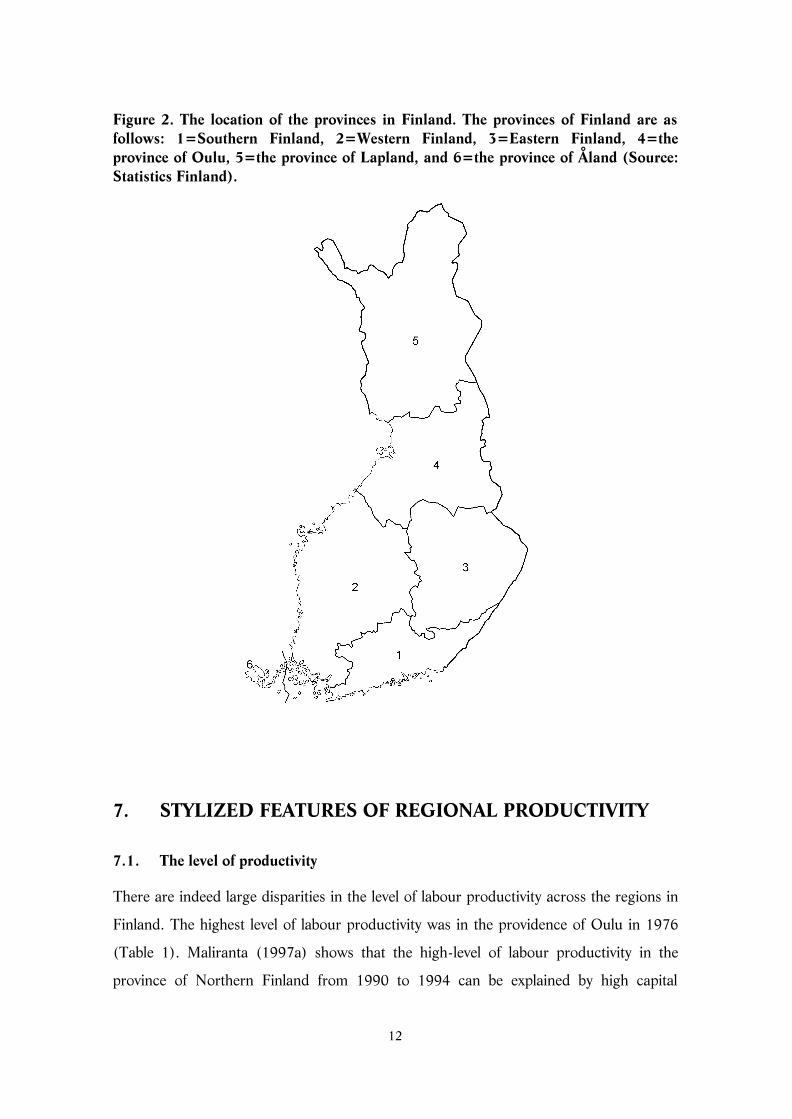
deviations from the input weighted industry-average in the year in question.12 Finland is

divided into six provinces (the so-called NUTS2-level in the European Union). Figure 2

shows the geographic location of these provinces in Finland.

12

Figure 2. The location of the provinces in Finland. The provinces of Finland are asfollows: 1=Southern Finland, 2=Western Finland, 3=Eastern Finland, 4=theprovince of Oulu, 5=the province of Lapland, and 6=the province of Åland (Source:Statistics Finland).

7. STYLIZED FEATURES OF REGIONAL PRODUCTIVITY

7.1. The level of productivity

There are indeed large disparities in the level of labour productivity across the regions in

Finland. The highest level of labour productivity was in the providence of Oulu in 1976

(Table 1). Maliranta (1997a) shows that the high-level of labour productivity in the

province of Northern Finland from 1990 to 1994 can be explained by high capital

13

intensity in the region. In contrast, the lowest level of labour productivity was in the

province of Eastern Finland in 1976.

There has been some convergence in labour productivity across regions during the past

few decades. Thus, the province of Eastern Finland has been able to perform better than

the province of Southern Finland in terms of labour productivity growth. The productivity

gap of Eastern Finland is therefore nowadays narrower with respect to the province of

Southern Finland than it used to be back in 1976. The process of convergence has been,

however, far from uniform. In particular, the province of Lapland has actually fallen

behind with respect to the province of Southern Finland.

The highest level of labour productivity was in the province of Oulu in 1999 (Table 2).

The level of labour productivity is about twenty per cent higher in the province of Oulu

than in the province of Southern Finland. The outstanding success of province of Oulu in

terms of labour productivity growth can most likely be explained by the cluster of

information technology that increased its share of value added within the Finnish

manufacturing industries during the 1990s. The ICT sectors have definitely been the main

strength of the recovery from the great slump of the 1990s (see IMF, 2001). In contrast,

the lowest level of labour productivity was in the province of Lapland in 1999.

7.2. The decompositions of productivity growth

The decompositions of productivity growth for incumbents reveal the underlying

dynamics and the heterogeneity at the plant level of the regions.13 These decompositions

indicate that the labour productivity growth rate was extremely rapid in the province of

Oulu during the past two episodes of this study (i.e. 1991–1994 and 1995–1999) (Table

3). In particular, in the province of Oulu, there was a strong positive contribution from

the so-called “between component” of the decomposition to the measure of labour

productivity growth, which constitutes a measure of restructuring between the plants of

the region. In other words, the population of relatively high-productivity plants expanded

its share of input usage in the province of Oulu during the 1990s. The most striking

finding is that this effect had an accelerating impact on labour productivity growth. The

dynamics that comes from the between component did not, therefore, dry up during the

recovery of the great slump of the early 1990s. In other words, there is no empirical

14

evidence for the “chill” in the pace of restructuring, as discussed by Caballero and

Hammour (2000), in the province of Oulu after the great slump of the early 1990s.

There is therefore empirical evidence that so-called creative destruction has played an

important role in the increase of labour productivity growth in the province of Oulu.

There was an increase in the between component in all other provinces of Finland during

the slump (i.e. 1991–1994), but the acceleration of restructuring between plants has, in a

way, melted away during the recovery. The province of Oulu is also highly interesting in

the sense that the contribution of between component to labour productivity growth was

negative during the episodes 1976–1980 and 1981–1985. Since then the situation has

turned upside down. In contrast to the situation in the province of Oulu, the contribution

of the between component to the rate of labour productivity growth was strongly negative

during the recovery of the Finnish economy (i.e. 1995–1999) in the province of Lapland,

but was, however, quite high during the slump of the early 1990s.

The decompositions further reveal that the so-called ”catching-up” term has been positive

in most provinces and during most episodes (Table 3). This pattern suggests that the

population of plants with low labour productivity has not been able to perform

exceptionally well in terms of the productivity growth rate. However, the results for TFP

(i.e. the negative values of the catching-up component) are in line with the conjecture that

there has been some convergence in performance through the above-average growth rates

among low productivity plants (Table 4).14

All in all, the empirical evidence strongly suggests that the evolution of the so-called

”between component” is the key to the understanding of the recent surge in labour

productivity growth of certain regions of Finland. In other words, the between component

has definitely been the proximate driving force of different fortunes of regions in terms of

the labour productivity growth rate during the 1990s. The decomposition of TFP growth

broadly reveals the same pattern. In particular, it should be noted that the between

component is generally higher when the input measure includes both labour and capital as

in the case of TFP (see Maliranta, 2001a). This pattern of adjustment suggests that the

reallocation of capital constitutes an important element of restructuring at the plant level

of the regions (see, e.g. Ramey and Shapiro, 1998).

15

7.3. The role of entry and exit

There is some role for the turnover of plants through the entry and exit of plants in the

determination of labour productivity growth in the regions of Finland despite the stylized

feature that restructuring among continuing plants has been a somewhat more important

driving force of productivity growth than net entry during the period of the investigation.15

There was, therefore, an increasing positive contribution from the exits of plants in the

provinces of Southern Finland, Western Finland, Eastern Finland and in the province of

Oulu, to the measure of labour productivity growth, during the years 1995-1999

compared with the period of depression (i.e. 1991-1994) (Table 3). In other words, these

provinces have been characterized by the process of exits of low productivity plants during

the recovery from the great slump of the early 1990s that has accelerated the growth rate

of labour productivity.16 In the province of Lapland, however, in contrast to this broad

pattern of adjustment, the contribution of exits of plants has been negative to the growth

rate of labour productivity during the years 1995–1999.

The decomposition of input-weighted TFP growth reveals a more complicated picture

(Table 4). Thus, the contribution of exits of plants was negative to the growth rate of TFP

even in the province of Oulu during the slump years of the early 1990s. When it comes to

the entry effect, the labour productivity indicator shows negative values usually, whereas

the TFP indicator more often suggests that entry has a positive effect on aggregate

productivity. This is to say that it seems to be important to control the use of capital input

when one is analysing entries since new plants initially seem to have initially relatively low

capital intensity and high capital productivity.

7.4. The evolution of productivity dispersions

The dispersion of labour productivity reveals other important aspects of the dynamics of

labour productivity growth (Table 5). In particular, one interesting pattern of the 1990s is

that there was a strong narrowing tendency in the dispersion of labour productivity among

plants in the province of Oulu and other provinces at the same time as there was an

accelerating positive contribution from the so-called “between component” to labour

productivity growth. These observations are nicely in line with the notion that there was

process-intensive restructuring in terms of the so-called “creative destruction” in the

Finnish regions during the 1990s, especially, in the province of Oulu.

16

In other words, the empirical evidence is in line with the thinking that the province of

Oulu has indeed been characterized by a process of cleansing of the fat left-hand tail of

low-productivity jobs that has yielded an increase in the growth rate of labour productivity

in that region. Regressions give additional support to the notion that an increase in the

magnitude of the so-called “between component” is certainly able to yield a compression

to the dispersion of input-weighted labour productivity at the plant level of the regions

(Table 6).17 In particular, the effect is realized with a lag of two years. This pattern of

productivity growth across regions was, in fact, already hinted at by the measures of gross

flows jobs and workers, which showed that there was a sharp rise in the rate of job

destruction in Eastern and Northern Finland compared with Southern Finland during the

slump of the early 1990s.

Table 1. The level of labour productivity in the provinces of Finland in 1976(Southern Finland=100).

Southern Finland 100.00Western Finland 116.50Eastern Finland 90.22Oulu 126.26Lapland 100.46

Table 2. The level of labour productivity in the provinces of Finland in 1999(Southern Finland=100).

Southern Finland 100.00Western Finland 95.43Eastern Finland 96.28Oulu 118.68Lapland 95.22

17

Table 3. The decomposition of the labour productivity growth rates amongincumbents, annual averages, % (and the contribution of entry and exit of plants).

1976–1980 1981–1985 1986–1990 1991–1994 1995–1999Southern FinlandAGGREGATE 3.10 4.20 6.35 3.74 2.97WITHBJ 2.50 2.77 4.96 1.44 2.74BETWBJ 0.42 0.72 1.19 1.63 0.98CATCHBJ 0.18 0.71 0.21 0.67 -0.76ENTRY -0.08 0.01 -0.23 -0.14 0.05EXIT 0.20 0.17 0.74 0.56 1.28

Western FinlandAGGREGATE 3.62 4.15 5.61 3.20 4.93WITHBJ 3.51 3.14 4.38 0.86 4.06BETWBJ -0.12 0.83 0.60 1.07 0.53CATCHBJ 0.23 0.18 0.63 1.28 0.34ENTRY -0.66 -0.35 -0.14 -0.35 -0.72EXIT 0.50 0.83 0.96 1.04 1.27

Eastern FinlandAGGREGATE 3.22 3.50 5.60 6.96 3.50WITHBJ 4.20 2.70 4.14 3.96 3.23BETWBJ 0.47 0.26 0.53 1.09 0.35CATCHBJ -1.45 0.55 0.93 1.90 -0.08ENTRY -0.24 -0.59 -0.64 -0.42 -0.93EXIT -0.30 0.52 1.36 1.15 1.85

OuluAGGREGATE 1.92 3.36 5.14 9.35 8.70WITHBJ 1.35 2.99 6.79 3.59 6.46BETWBJ -0.49 -0.64 0.60 1.00 2.00CATCHBJ 1.07 1.02 -2.25 4.75 0.24ENTRY -1.09 -0.55 0.10 -0.31 -1.94EXIT 1.14 0.86 0.59 1.09 1.82

LaplandAGGREGATE 4.15 1.80 10.82 6.28 1.86WITHBJ 5.56 1.18 8.51 5.20 1.18BETWBJ -0.47 0.30 0.03 1.58 -1.48CATCHBJ -0.94 0.32 2.29 -0.50 2.15ENTRY -0.91 -0.54 -0.88 -0.94 -1.12EXIT 0.65 1.11 1.24 2.89 -1.18

18

Table 4. The decomposition of TFP growth rates among incumbents, annual averages,% (and the contribution of entry and exit of plants).

1976–1980 1981–1985 1986–1990 1991–1994 1995–1999Southern FinlandAGGREGATE -0.21 0.65 2.28 2.33 0.28WITHBJ -0.21 -0.55 0.95 1.81 0.93BETWBJ 1.36 1.08 1.35 2.35 1.29CATCHBJ -1.36 0.11 -0.02 -1.83 -1.95ENTRY 1.01 0.45 0.47 0.84 0.64EXIT 0.17 -0.17 -0.06 -0.07 -0.13

Western FinlandAGGREGATE 0.31 0.82 1.96 1.94 2.00WITHBJ 0.79 -0.03 1.33 0.61 1.74BETWBJ 1.17 0.85 1.31 1.67 1.60CATCHBJ -1.65 -0.01 -0.67 -0.34 -1.34ENTRY 0.68 0.25 0.93 0.46 0.62EXIT 0.18 0.40 0.17 0.10 -0.06

Eastern FinlandAGGREGATE 0.09 0.63 2.95 5.01 0.79WITHBJ 2.46 -0.51 1.67 6.30 1.06BETWBJ -0.13 1.35 1.74 0.62 0.55CATCHBJ -2.24 -0.20 -0.47 -1.91 -0.82ENTRY 0.46 0.20 0.42 0.36 0.84EXIT -0.68 0.10 0.11 0.35 0.51

OuluAGGREGATE 0.65 1.01 3.04 7.24 2.42WITHBJ -0.74 0.13 4.61 5.11 1.04BETWBJ 0.64 0.22 1.74 2.77 1.49CATCHBJ 0.75 0.66 -3.32 -0.64 -0.11ENTRY 0.50 0.12 0.90 0.26 0.68EXIT -0.08 0.33 -0.27 -0.25 0.72

LaplandAGGREGATE 6.80 0.62 4.28 11.76 -1.58WITHBJ 8.81 -0.10 2.74 14.15 -1.79BETWBJ 0.65 0.89 1.12 1.73 1.42CATCHBJ -2.66 -0.17 0.42 -4.12 -1.21ENTRY -2.07 0.02 0.30 0.32 0.17EXIT -0.08 0.23 0.01 0.01 0.26

19

Table 5. The dispersion of labour productivity among incumbents.

1976–1980 1981–1985 1986–1990 1991–1994 1995–1999Southern FinlandSTDLNPL 65.30 70.89 68.36 66.75 61.10P50-P10 68.23 75.22 67.85 65.68 54.01

Western FinlandSTDLNPL 60.76 66.71 64.81 66.44 55.48P50-P10 68.90 73.40 71.49 70.12 52.65

Eastern FinlandSTDLNPL 63.28 62.01 58.49 75.75 54.68P50-P10 142.59 131.88 133.10 145.46 125.75

OuluSTDLNPL 69.63 78.88 66.99 74.76 64.44P50-P10 155.00 167.71 152.30 173.24 149.22

LaplandSTDLNPL 62.11 73.65 69.95 90.58 67.15P50-P10 73.03 68.49 58.69 67.05 44.98

Notes: STDLNPL refers to the standard deviation of the logarithm of labour productivity across plants.The dispersion measures are input weighted. P50-P10 refers to the difference between 50th percentileand 10th percentile of logarithm labour productivity across plants.

Table 6. The estimation results for the determination of dispersion of labourproductivity across plants (dependent variable: the difference in the standard deviationof logarithm of labour productivity across plants).

Model 1 Model 2Variables Coefficients t-statistics Coefficients t-statistics

BETWBJ 1.24 3.52 3.14 1.57BETWBJ (t-1) 0.77 1.35 1.54 0.72BETWBJ (t-2) -2.59 -4.38 -5.31 -2.67CATCHBJ .. .. 0.60 0.96CATCHBJ (t-1) .. .. 0.14 -0.21CATCHBJ (t-2) .. .. -1.34 -2.08

AR(1) -0.47 0.47Number of observations 100 100

Notes: The models are estimated over the period from 1976 to 1999 by GLS, in whichheteroskedasticity with cross-sectional correlation and common AR(1) is allowed. Model 1 is estimatedwith the dummy variables that are attached to years and provinces. The same results as reported asModel 1 hold when the model is estimated by including a common trend across provinces or when themodel is estimated without any controls for the variation that arises from the years from 1976 to 1999.Model 2 is estimated with trends that are specific to the provinces of Finland.

20

8. EXPLANING REGIONAL DIFFERENCES

By using decompositions of the productivity growth rate, we have discovered that the

between component has been an extremely important element in the acceleration of

regional productivity growth since the 1980s. This source of aggregate economic growth

deserves some extra notice, as it calls for job creation and destruction and the

concentration of investments into certain plants characterised by high labour and capital

productivity. Moreover, we have shown that this factor of growth is related to the

development of productivity dispersion within the Finnish regions, which, in turn, seems

to be associated with wage dispersion (see Dunne, Haltiwanger and Troske 2000;

Maliranta, 2001b).

These notions invite us to explore the economic fundamentals that are behind the

evolution of the between component of regional labour productivity growth

decomposition. In particular, we investigate, in the following, the determination of the

between component by explaining it by means of a vector of the economic fundamentals

that includes the export shares (the variable EXPSH) and a measure of R&D-intensity

(the variable R&D) of the Finnish provinces during the past few decades.

The motivation for these variables emerges from the notion that the export share is a

proxy variable for exposure to competition from foreign markets. In particular, the

recovery from the great slump of the early 1990s was indeed an export-led expansion.

This means that exposure to competition from foreign markets most likely shaped the

pace of evolution of restructuring in the Finnish regions during the 1990s. Investments in

research and development are likely to be an important catalyst for the reorganization and

the reallocation of scarce resources in the population of plants within regions. This feature

means that there should therefore be more turbulence in the provinces measured by the

between component that have a high R&D intensity compared with the rest of the regions.

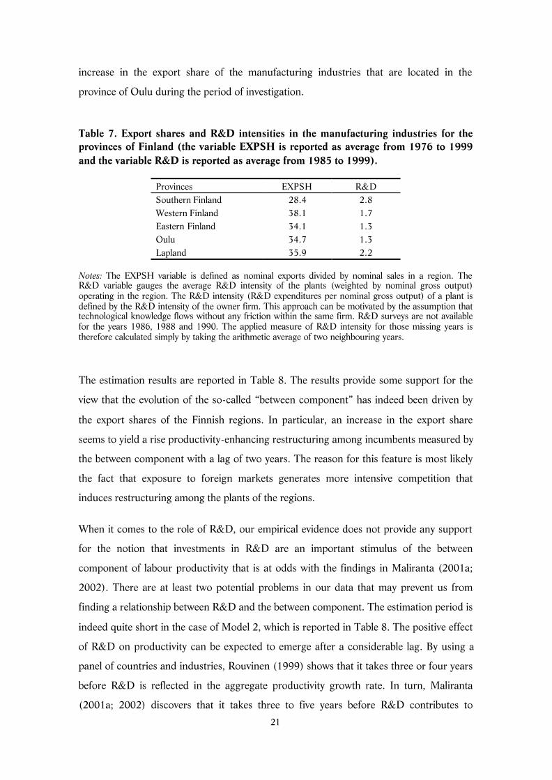
The export shares and the R&D intensities of the Finnish provinces are reported in Table

7. The export share of the manufacturing industries is at its lowest level and the R&D

intensity of the Finnish regions is at its highest level in the province of Southern Finland.

However, these average figures mask, for instance, the fact that there has been a rapid

21

increase in the export share of the manufacturing industries that are located in the

province of Oulu during the period of investigation.

Table 7. Export shares and R&D intensities in the manufacturing industries for theprovinces of Finland (the variable EXPSH is reported as average from 1976 to 1999and the variable R&D is reported as average from 1985 to 1999).

Provinces EXPSH R&DSouthern Finland 28.4 2.8Western Finland 38.1 1.7Eastern Finland 34.1 1.3Oulu 34.7 1.3Lapland 35.9 2.2

Notes: The EXPSH variable is defined as nominal exports divided by nominal sales in a region. TheR&D variable gauges the average R&D intensity of the plants (weighted by nominal gross output)operating in the region. The R&D intensity (R&D expenditures per nominal gross output) of a plant isdefined by the R&D intensity of the owner firm. This approach can be motivated by the assumption thattechnological knowledge flows without any friction within the same firm. R&D surveys are not availablefor the years 1986, 1988 and 1990. The applied measure of R&D intensity for those missing years istherefore calculated simply by taking the arithmetic average of two neighbouring years.

The estimation results are reported in Table 8. The results provide some support for the

view that the evolution of the so-called “between component” has indeed been driven by

the export shares of the Finnish regions. In particular, an increase in the export share

seems to yield a rise productivity-enhancing restructuring among incumbents measured by

the between component with a lag of two years. The reason for this feature is most likely

the fact that exposure to foreign markets generates more intensive competition that

induces restructuring among the plants of the regions.

When it comes to the role of R&D, our empirical evidence does not provide any support

for the notion that investments in R&D are an important stimulus of the between

component of labour productivity that is at odds with the findings in Maliranta (2001a;

2002). There are at least two potential problems in our data that may prevent us from

finding a relationship between R&D and the between component. The estimation period is

indeed quite short in the case of Model 2, which is reported in Table 8. The positive effect

of R&D on productivity can be expected to emerge after a considerable lag. By using a

panel of countries and industries, Rouvinen (1999) shows that it takes three or four years

before R&D is reflected in the aggregate productivity growth rate. In turn, Maliranta

(2001a; 2002) discovers that it takes three to five years before R&D contributes to

22

aggregate productivity through plant-level restructuring. The second problem is that our

regional R&D-intensity measure may be inaccurate.

Table 8. The estimation results for the determination of the between component for theprovinces of Finland (dependent variable: betwbj).

Model 1 Model 2Variables Coefficients t-statistics Coefficients t-statistics

EXPSH -0.11 -2.76 -0.03 -1.97EXPSH (t-1) -0.01 -0.32 .. ..EXPSH (t-2) 0.08 7.69 .. ..R&D .. .. -0.34 -1.71R&D (t-1) .. .. 0.08 0.44

AR(1) 0.06 -0.01Number of observations 100 70

Notes: The models are estimated by GLS, in which heteroskedasticity with cross-sectional correlationand common AR(1) is allowed. Model 1 is estimated over the period from 1976 to 1999 with thedummy variables that are attached to years. The results remain the same when the dummy variables tothe provinces of Finland are also attached to Model 1. Model 2 is estimated from 1985 to 1999 with thedummies that are attached to the provinces of Finland.

9. CONCLUSIONS

The aim of the study was to decompose the regional productivity growth rate in the

Finnish provinces by using detailed plant-level data from 1975 to 1999. The results show

that there was an extremely strong performance in terms of labour productivity growth in

the province of Oulu during the 1990s and an increasing part of labour productivity

growth in the province of Oulu can be explained by the reshuffling of the input shares

among incumbent plants.

The evolution of the so-called ”between component” of productivity growth

decompositions is therefore the key to the understanding of the recent surge in labour

productivity growth in certain parts of Finland. In other words, there is empirical evidence

in favour of the perspective that so-called creative destruction shaped the evolution of the

labour productivity growth rate across the regions of Finland during the 1990s. The

acceleration of productivity growth through plant level restructuring has indeed entailed

23

compression of productivity dispersion between plants within regions. In turn, there is

empirical evidence that the development of the so-called ”between component” has been

driven by the export shares of the regions. In particular, an increase in a region’s export

share seems to generate a reallocation of inputs among incumbent plants in a

productivity-enhancing way.

REFERENCES

Abowd, J.M. and F. Kramarz (1999). “The analysis of labor markets using matched employer-employee data.” In Handbook of Labour Economics, Vol. 3B, 2629–2710. Eds. O. Ashenfelter andD. Card. Amsterdam: North-Holland.

Bartelsmans, E.J. and M. Doms (2000). “Understanding productivity: lessons from longitudinalmicrodata.” Journal of Economic Literature XXXVIII, 596–594.

Bernard, A. B. and C.I. Jones (1996). “Productivity across industries and countries: time seriestheory and evidence.” The Review of Economics and Statistics LXXVII, 135–145.

Böckerman, P. (2002). “Understanding regional labour productivity in a Nordic welfare state:does ICT matter?”. Discussion Papers, 798. The Research Institute of the Finnish Economy.

Böckerman, P. and M. Maliranta (2001). “Regional disparities in gross job and worker flows inFinland.” Finnish Economic Papers 14, 83–104.

Caballero, R.J. and M.L. Hammour (1994). “The cleansing effect of recessions.” The AmericanEconomic Review 5, 1350–1368.

Caballero, R.J. and M.L. Hammour (2000). “Institutions, restructuring, and macroeconomicperformance.” Unpublished. MIT.

Davis, S.J., and J. Haltiwanger (1999). “Gross job flows.” In Handbook of Labour Economics,Vol. 3B, 2711–2805. Eds. O. Ashenfelter and D. Card. Amsterdam: North-Holland.

Dunne, T., J. Haltiwanger, and L. Foster (2000), “Wage and productivity dispersion in U.S.manufacturing: the role of computer investment.” Working Papers 7465. National Bureau ofEconomic Research.

Foster, L., J. Haltiwanger and C. J. Krizan (2001). ”Aggregate productivity growth: lessons frommicroeconomic evidence.” In New Developments in Productivity Analysis. Studies in Income andWealth Volume 63. Eds. C.R. Hulten, E.R. Dean and M.J. Harper. Chicago: The University ofChicago Press.

IMF (2001). Finland: Selected Issues.

Kangasharju, A., and S. Pekkala (2001). “Regional economic repercussions of an economiccrisis: a sectoral analysis.” Discussion Papers 248. Government Institute for Economic Research.

Kiander, J., and P. Vartia (1996). “The great depression of the 1990s in Finland.” FinnishEconomic Papers 1, 72–88.

Krugman, P. (1994). The Age of Diminished Expectations. Cambridge, MA.: The MIT Press.

Lehto, E. (2000). “Regional impacts of R&D and public R&D funding.” Studies 79. LabourInstitute for Economic Research.

24

Loikkanen, H.A., A. Rantala and R. Sullström (1998). “Regional income differences in Finland,1966–96.” Discussion Papers 181. Government Institute for Economic Research.

Mairesse, J., and E. Kremp (1993). “A look at productivity at the firm level in eight Frenchservice industries.” Journal of Productivity Analysis 4, 211–234.

Maliranta, M. (1997a). “Plant productivity in the Finnish manufacturing. Characteristics of highproductivity plants.” Discussion Papers 612. The Research Institute of the Finnish Economy.

Maliranta, M. (1997b). ”Productivity performance in regions. Some findings from Finnishmanufacturing.” Unpublished. The Research Institute of the Finnish Economy.

Maliranta, M. (1997c). “Suomen, Yhdysvaltojen ja Ruotsin metalliteollisuuden tuottavuusver-tailu.” (In Finnish). In Metalliteollisuuden tuottavuus kansainvälisestä näkökulmasta, Eds. METand McKinsey & Company. Helsinki: Metalliteollisuuden Keskusliitto.

Maliranta, M. (2001a). “Productivity growth and micro-level restructuring. Finnish experiencesduring the turbulent decades.” Discussion Papers 757. The Research Institute of the FinnishEconomy.

Maliranta, M. (2001b). “Tuottavuutta mikrotason rakennemuutoksesta.” (In Finnish). TheResearch Institute of the Finnish Economy, Suhdanne 2/2001, 80–83.

Maliranta, M. (2002). “From R&D to productivity through plant-level restructuring.” DiscussionPapers 795. The Research Institute of the Finnish Economy.

Ramey, V.A. and M.D. Shapiro (1998). “Capital churning.” Unpublished. University ofCalifornia, San Diego, Department of Economics.

Rigby, D.L. and J. Essletzbichler (2000). “Impacts of industry mix, technological change,selection and plant entry/exit on regional productivity growth.” Regional Studies 34, 333–342.

Rouvinen, P. (1999). “Issues in R&D-productivity dynamics: causality, lags, and dry holes.”Discussion Papers 694. The Research Institute of the Finnish Economy.

Schumpeter, J.A. (1942). Capitalism, Socialism, and Democracy. Harvard: Harper and Row.

Susiluoto, I. and H.A. Loikkanen (2001). “Seutukuntien taloudellinen tehokkuus 1988–1999”.(in Finnish). Research Series 2001:9. City of Helsinki Urban Facts.

25

________________________________________

1 Kiander and Vartia (1996) provide a description of the great slump of the 1990s in Finland.

2 To take an example, the province of Kainuu (defined at the NUTS3 level of the European Union) is apart of the province of Oulu in the following decomposition of productivity growth in the regions ofFinland. This means that the following investigation emphasizes the view that there was a great deal ofreallocation of scarce resources within the provinces in Northern Finland during the 1990s.

3 Bartelsman and Doms (2000), and Foster, Haltiwanger, and Krizan (2001) provide detailed surveys ofthe literature that have investigated the evolution of productivity growth at the plant level of the economyby using these kind of decompositions.

4 Nominal output figures are converted into the end-year (t) prices by using the producer’s price indexat the 2- or 3-digit industry level when computing productivity changes between pairs of successiveyears. In this way, we avoid a fixed base year bias that will arise if a certain fixed base year is used anddifferent price indexes are used for plants in different industries (see Maliranta, 2001a).

5 The effect arising from entrants and exitors (net entry) can be measured by substracting the aggregateproductivity growth rate among incumbents from the total aggregate productivity growth rate. This isthe aggregate productivity growth rate among all plants. Thus, the total aggregate productivity growthrate is net entry plus productivity growth components among incumbents (see Maliranta 1997b; 2001).

6 The name of this variable is due to the fact that it is the between component obtained by a modifiedversion of the formula presented by Bernard and Jones (1996).

7 The conclusion on the entries and exits of plants is based on the successive, pair-wise comparisions ofproductivity from year to year. The role of entries and exits of plants for the growth rate of productivitynaturally increases as the time-horizon of the comparisions extends.

8 Regarding the empirical evidence, see Maliranta (2001a).

9 Catching up component (catchbj) is a term that is obtained by reformulating the decompositionformula presented by Bernard and Jones (1996) (see Maliranta, 2001a).

10 If the relative productivity levels across size groups are reasonably stable over time, short-termvariation in this component may reveal something interesting about the changes in the economicenvironment. This term can be expected to be low when the productivity-improving adjustment amonglow productivity plants is common.

11 For robustness of the reported results, we have examined how sensitive the patterns of the dispersionseries over time are to changes in the cut-off limit from 5 to 20 in the period 1975–1994. It turns outthat patterns are indeed quite similar.

12 In addition to this we have dropped 8 influential observations from those plants, about 10 000 innumber, that appear at least once in the period from 1975 to 1998 when one is calculating total factorproductivity components (14 in labour productivity computations). They have clearly erroneousinformation that is reflected, for example, so that the absolute values of between and catching up termsof equation (4) are quite large and have opposite signs.

13 Rigby and Essletzbichler (2000) provide the decompositions of labour productivity growth for the USstates over the period from 1963 to 1992.

14 The assumption that the size and productivity level are uncorrelated among plants is more realistic inthe case of TFP than labour productivity so that our catching up component can be expected to capturebetter the negative correlation between the productivity level and the growth rate (with a negative value)(see discussion in Maliranta, 2001a, 30–31).

26

15 An important feature of the calculations is that this conclusion is based on the successive, pair-wisecomparisions of productivity from year to year.

16 It is worth noting that high positive exit components appear in the latter part of the 1990s, which wasa period of strong growth in Finland.

17 The variable catchbj gets a negative sign in the regressions. This result is in conflict with the notionthat the ‘catching up effect’ should work in the same direction as the external restructuring implied bythe between component.