The Michigan Recreational Angling Demand Model

BY

Frank Lupi , John P. Hoehn , Heng Zhang Chen , and Theodore D. Tomasi

March, 1998

Staff Paper Number 97-58, Department of Agricultural Economics, Michigan State University.

Copyright © 1998 by Frank Lupi, John P. Hoehn, Heng Zhang Chen and Theodore D. Tomasi. Allrights reserved. Readers may make verbatim copies of this document for non-commercial purposes by any means, provided that this copyright notice appears on all such copies.

The Michigan Recreational Angling Demand Model

BY

Frank Lupi ,1 John P. Hoehn ,1 Heng Zhang Chen ,2 and Theodore D. Tomasi 3

March, 1998

Corresponding author: Frank Lupi,1 (phone: 517/432-3883; fax: 517/432-1800; e-mail: lupi@pilot.msu.edu)

Acknowledgements: We thank Douglas B. Jester for sharing his experience with and knowledge of Michiganangling. We have benefited from the insights and previous work of Carol A. Jones. We also thank Wiktor L.Adamowicz, Richard T. Carson, W. Michael Hanemann, Edward R. Morey, George Parsons, and W. DouglassShaw for their valuable input during the project development. We are grateful to the Michigan Departments ofNatural Resources and Environmental Quality for supporting this research. We also thank Larry Hembroff andthe staff of the Survey Research Division at Michigan State University for their efforts on the survey. The authorsare solely responsible for the contents of this work. __________________________

1 Department of Agricultural Economics, Michigan State University, East Lansing, MI 48824-1039; 2 American Express Travel Related Services, 10400 North 25th Avenue, Phoenix, AZ 85021; and 3 College of Marine Studies, 309 Robinson Hall, University of Delaware, Newark, DE 19716.

The Michigan Recreational Angling Demand Model

Recreational demand models based on the travel cost method are widely used to establish the

economic use-value of water based recreation. Modern multiple-site variants of the travel cost method allow

the spatial patterns of recreation demand to be linked to quality characteristics of recreation sites. This

linkage can be used to estimate values of changes in site characteristics such as water quality. The most

widely used type of multiple-site travel cost model is the random utility model which was popularized as a

recreation demand model by the work of Bockstael, Hanemann, and Strand, and Bockstael, Hanemann,

and Kling.

This paper reports on a large-scale spatial model of the demand for recreational angling in

Michigan. The model is a repeated random utility model (RUM) of recreational fishing in Michigan by

resident anglers. The model was developed at Michigan State University (MSU) under a grant from

Michigan's Department of Natural Resources (MDNR) and Department of Environmental Quality. The

material in this paper summarizes, and is drawn from, the project report of Hoehn, Tomasi, Lupi, and Chen.

The model differs from others in the literature in its breadth and scale. The geographic scope of the model

is the entire state of Michigan, and the model encompasses the broad range of fishing activities available

in a state with abundant water and fishery resources. Because descriptions of the theory of the RUM and

the statistical models used here are readily available in the literature (McFadden, 1981; Ben-Akiva and

Lerman; Morey), the exact specification of the site choice probabilities and the likelihood function are

relegated to the Appendix. Instead, our focus is on describing the model structure, presenting estimated

parameters, and providing some illustrative results.

Model Structure

The MSU model is a nested repeated random utility travel cost model that permits a wide variety

of trip types. In the MSU model, trips are distinguished by trip duration, target species, water body, and

destination. Single-day and multiple-day trips are treated as separate types of trips. Fishing trips targeting

MSU Model: Page 1

warm-water species such as walleye and bass are differentiated from trips targeting cold-water species such

as trout and salmon. Fishing at Great Lakes, inland lakes, and inland rivers are treated as distinct types

of trips. Finally, trips are distinguished by the destination county for the fishing trip. Thus, the model

distinguishes between several distinct fishing opportunities available in any given county in Michigan, as

well as distinguishing among counties in Michigan.

Two categories of trip duration, single-day trips and multiple-day trips, were chosen to make the

best use of the available data. Less than 20% of the trips reported by survey respondents were multiple-

day trips. The MSU team determined that it was important to allow the estimated site quality parameters

to differ by trip lengths. The team also sought to keep the distinctions between fish species and water body

types within each trip length (discussed below). As a result, there were not enough multiple-day trip

observations to further subdivide them into additional trip length categories while maintaining the site,

species, and water body distinctions mentioned above.

Within either the single-day or multiple-day trip length, the different types of fishing trips are called

“product lines.” Each product line (PL) describes a generalized combination of water body type (Great

Lakes, inland lakes, and river/streams) and fish species (cold and warm-water species), plus anadromous

runs. This follows Jones and Sung who use a similar structure in their earlier RUM for Michigan fishing.

Based on factor-analytic work by Kikuchi, they categorize fishing activities into seven product lines: (1)

Great Lakes warm species, GLwarm; (2) Great Lakes cold species, GLcold; (3) inland lakes warm species,

ILwarm; (4) inland lakes cold species, ILcold; (5) river and streams warm species, RSwarm; (6) river and

streams non-anadromous cold species, RScold; and (7) river and streams anadromous species, Anad.

Cold-water species include salmon and trout, and warm-water species include bass, yellow perch,

panfish, walleye, and pike. In addition, species on anadromous runs are separated from other cold-water

river species; anadromous run species include salmon and steelhead. Each of the product lines is available

as a single-day trip and as a multiple-day trip. As a result, there are seven fishing product lines within each

trip length.

MSU Model: Page 2

The sites within each product line are the counties that offer fishing opportunities within that product

line. For the Great Lakes product lines, the sites are the stretch of Great Lake shoreline in the county.

Each of Michigan's 83 counties can appear several different places as a site in the model. For example,

consider a Great Lake county with anadromous runs, warm and cold inland lakes, and with warm and cold

inland streams. Such a county would support all seven product lines. Moreover, these seven types of

fishing would be available for single and multiple-day trips. Thus, the county would appear in fourteen

separate places in the model. Each of the 14 types of trips to this site (county) is treated as a distinct

fishing opportunity in the model. The number of counties that are feasible for each PL are: 41 in GLcold,

40 in GLwarm, 83 in ILwarm, 67 in ILcold, 83 in RSwarm, 69 in RScold, and 44 in Anad. Combining these

with the two trip durations yields 854 combinations of trip and site types that are in the model.

In a RUM type model, the set of sites which can be chosen is called the feasible choice set. The

feasible choice set in the MSU model varies across individuals and over time. The choice set varies over

time because the anadromous run PL is not available during the summer months. The choice set varies

for individuals because there is a constraint on how far an individual can travel for a particular trip length.

The choice set for day trips is composed of feasible counties within 150 miles of an individual's permanent

residence. From the survey data, only about two percent of the observed one-day trips exceed the 150

miles limit. The choice set for multiple-day trips consists of feasible counties within 600 miles of an

individual's permanent residence -- the maximum observed one-way driving distance in the sample. Due

to the distance constraint, each individual has about 600 feasible fishing activity/site combinations to choose

from on each choice occasion with about 60 fewer feasible alternatives in the summer months when

anadromous runs are not available.

Choice Occasions: The MSU model is a repeated RUM, where the season is divided into a series

of choice occasions (Carson and Hanemann; Morey, Rowe, Watson). During each choice occasion, anglers

decide whether or not to fish. The decision to fish or not is then made anew at each occasion. The length

of the season and the length of a choice occasion jointly determine the number of choice occasions in a

season. The MSU model considers only those trips made during the “open water” fishing season, defined

MSU Model: Page 3

as the period from April 1 to October 31. While the determination of the season length is straightforward,

many factors affect the selection of the length of the choice occasion. The more choice occasions there

are and the larger the number of choices per occasion, the greater the computational burden of the model.

On the other hand, if the model contains few choice occasions, there will be some individuals who have

taken more trips than there are choice occasions, and some of their trips will need to be "trimmed" from

the data. For example, Morey, Rowe, and Watson choose 50 choice occasions for their study of fishing

in Maine noting that data was trimmed for the few individuals that had more than 50 trips.

As mentioned, the MSU model permits two trip lengths, single-day trips and multiple-day trips, with

at most one trip per choice occasion. The decision to partition the trip length into two categories takes into

consideration the limited number of multiple-day trip observations across the seven product lines. Also,

partitioning the trip lengths into finer grids greatly increases computational burden -- for the MSU model,

each additional trip length category adds 427 site/product line combinations to each choice occasion. For

the research reported here, the length of the choice occasion was set at 3.5 days, or two choice occasions

per week. This period was selected because about 96% of all trips were for 4 days or less (3 nights away

or less). Of the multiple-day trips, about 80% lasted three nights or less with the average nights away being

just less than three. Thus, by setting the choice occasion length at 3.5 days, most of the multiple-day trips

"fit" into the choice occasion period.

In the MSU model, catch rates vary by month. Time-varying quality attributes such as these are

easily accommodated in the repeated RUM framework. Since catch rates vary monthly, the month of a trip

must be known in order to estimate the model. In this sense, the number of trips and choice occasions per

month is what drives the data trimming decisions in the MSU model. If there are more trips in any month

than there are choice occasions in that month, excess trips must be trimmed. For the MSU model, with

the choice occasion length at 3.5 days there are 8 to 9 choice occasions in any month with a total of 61

occasions for the season. For any individual in the sample, if the sum of their reported single-day and

multiple-day trips in any month exceeds the number of choice occasions in that month, a random selection

of the trips are trimmed so that the month contains no more trips than the number of choice occasions in

MSU Model: Page 4

that month. Less than 2% of the reported trips in any month exceeded the number of choice occasions

in that month, and in most months less than 1% of the trips were trimmed.

Nesting Structure: The MSU statistical model is specified as a four-level nested-logit (see Morey

or McFadden, 1981). This specification permits the error terms for alternatives within groups (nests) to be

more correlated with one another than with alternatives in other groups partially relaxing the more restrictive

substitution patterns of multinomial logit. The nesting structure closely resembles the types of fishing

activities in the MSU model. The first level distinguishes among participation and non-participation, the

second level differentiates by trip duration, the third involves the product lines, and the bottom level is for

specific sites (see Figure 1). Bear in mind that the nesting structure is simply a way of grouping elemental

alternatives that are likely to be similar to one another. Whether the alternatives really are similar or not

is revealed during the model estimation.

Also note that in the nesting structure used in the MSU model, the inland lakes, rivers and streams,

and anadromous run categories have been further subdivided to distinguish whether the site is in a county

that has Great Lakes shoreline. Here the Jones and Sung nesting structure has been extended for non-

Great Lakes product lines to distinguish between counties that do and do not have Great Lakes shoreline.

This was a particularly important effect for multiple-day trips. Unlike the product line designation, the

shoreline distinction is mutually exclusive; a county is either in the group of counties that contain Great Lake

shoreline or it is not. The nesting at the PL level simply subdivides the existing PLs. As a result, within

each trip length there are a total of twelve nested groups corresponding to shoreline and product line

combinations. The twelve combinations are illustrated in Figure 1.

Variables

In this section, the variables and their measurement are briefly described. The discussion begins

with the trip price variable (travel cost). Travel costs are the sum of driving, lodging, and time costs. To

the extent possible, the travel costs were tailored to the individual sample members.

MSU Model: Page 5

Driving Cost Regression and Prediction: Driving costs per mile were calculated using a regression-

based prediction of per mile fuel costs plus a per mile depreciation charge. Predicted fuel costs vary across

individuals in the model. The dependent variable in the fuel cost regression was the reported fuel cost for

the fishing trip. The equation itself was specified as a tobit model with multiplicative heteroskedasticity

(Greene 1993, p. 598). The explanatory variables were distance (the round-trip distance) and three

variables interacted with distance: share, tow, and truck which represented whether or not expenses were

shared with other households, whether a boat was towed, and whether the vehicle was a truck or camper.

The distance, tow, and truck variables were significant in explaining fuel costs, while the truck and share

variables were significant in explaining heteroskedasticity. The fuel cost data was collected for a subset

of trips (the first trip in each interview of the panel survey). The regression was estimated using the subset

of these data that met several conditions aimed at minimizing any possible errors in the measurement of

the travel distance. For example, the regression only used fuel costs data for single-day, single-site trip

with a primary purpose of fishing. In all, there were 828 observations for the regression.

For the repeated RUM, one needs to predict what the travel cost would be for all choice occasions

regardless of whether a trip was actually taken. The fuel regression was used to predict fuel costs for all

choice occasions by using each individual's response to questions about their "usual" travel behavior as

explanatory variables. Specifically, individuals were asked about their usual vehicle type, whether or not

they usually towed a boat, and whether they usually shared expenses with other households. Their

answers to these questions yield the explanatory variables for fuel cost predictions for all choice occasions.

The complete per mile vehicle cost was calculated by adding to each individual's predicted fuel cost

a 14.1 cent per mile depreciation charge, based on the AAA depreciation charge of $141 for each 1,000

miles in excess of 15,000 miles driven annually for a full size passenger vehicle (AAA 1993). This figure

does not take into account annual depreciation based on normal driving. Nor does it include any of the

fixed costs of vehicle ownership such as insurance. The charge is aimed at capturing the marginal cost

of depreciation. Table 1 presents some summary statistics for the predicted per mile driving costs.

MSU Model: Page 6

Figure 1: Four Level Nesting Structure for Each Choice Occasion: Participation, Trip, Product Line, and Site Levels.

MSU Model: Page 7

Lodging Cost: For each overnight trip, respondents were asked about actual lodging types and

Table 1: Summary of Predicted Values for Individual Specific Cost Variables.

Percentiles

Predicted values † Mean Std. dev. Min. 10% 25% 50% 75% 90% Max

Hourly wage rate 15.2 5.2 5.5 9.6 11.6 14.2 17.9 22.0 42.9

Per mile driving cost 0.25 0.03 0.216 0.216 0.216 0.247 0.259 0.285 0.29

Per night lodging cost 19.2 11.1 13.1 13.3 14.6 14.6 16.5 47.2 47.2

† N = 1,902 cases with complete panel data

lodging costs. The average per-night lodging costs are based on the sample average per night cost of

lodging for four types of lodging: camping, hotel, cabin, and other. "Other" includes activities such as

staying on a boat, fishing all night long, and staying in the car. Individuals were assigned the per night cost

that corresponded to the type of lodging that they indicated they usually use when they take overnight trips.

The per night costs were multiplied by 3 to reflect the cost of lodging for an average multi-day trip. Lodging

costs are zero for single-day trips. Table 1 provides summary statistics for the predicted lodging costs.

Time Cost/Wage Estimation: Time costs are the predicted value of an individual's time multiplied

by the time for the trip length. It was assumed that one-day trips require 8 hours of time and multi-day trips

use 3.5 eight hour days or 28 total hours of time. These are based on an assumed 12 hours of available

work time per day deflated by 2/3 for an after-tax rate (or 8 hours a day with no tax rate). The predicted

value of an individual's time came from a regression of wages on demographic variables. A shadow wage

equation which accounted for the potential differences between time values and wages for individuals with

fixed work hours was tested, but it did not significantly outperform the wage equation (Lupi et al.). The

wage regression was specified as a semi-log model with multiplicative heteroskedasticity. The semi-log

form was based on the work of Phagan and follows a long tradition in labor economics.

The wage variable was derived from the employment information collected in the survey. For

individuals who worked on an hourly basis, wage was specified as their reported wage rate. For those who

were on a salary, wage was derived by dividing their annual salary by their annual hours worked. In an

effort to increase the accuracy of the derivation of hours worked per year, annual hours worked was

MSU Model: Page 8

calculated using information on the months and hours per week that the respondent worked. The

independent variables used in the wage regression were years of education, age, gender, experience, the

number of kids in the household, the number of adults in the household, and a dummy variable for those

who live in the Detroit metro counties of Monroe, Oakland, and Wayne. Experience was defined as age

minus years of education minus six. The adults and kids variables were not significant in explaining log

wages or the heteroskedasticity. All other variables were significant in both portions of the wage model.

Table 1 presents some summary statistics for the predicted wages.

Site Quality Variables: This section briefly describes the variables which are used to describe the

quality of elementary site alternatives. Catch rates for various species in the GL warm, GL cold, and Anad

product lines are included in the model. In the GL warm product line, catch rates were computed for yellow

perch, walleye, northern pike, bass (which includes smallmouth bass, largemouth bass, bluegill, and

pumpkinseed), and carp (which includes carp, freshwater drum, catfish, and suckers). In GL cold, catch

rates are included for chinook salmon, coho salmon, lake trout, and rainbow trout. For the Anad product

line, catch rates are included for chinook salmon, coho salmon, and rainbow trout. These catch rates were

computed from MDNR creel survey data from the late 1980s and were employed by Jones and Sung.

Specifically, catch rate equations were estimated by species for sites with creel data, and this equation was

used to predict catch rates at all sites. These were Poisson regressions for count data, implemented by

Douglas Jester, MDNR. Predicted catch rates vary monthly throughout the open-water season.

In the IL warm product line, the total surface area (in acres) of warm-water inland lakes within the

county is included in the model. Similarly, for the IL cold product line, the total surface area (in acres) of

cold-water lakes within the county is included. The acres for two-story lakes, with warm water on top and

cold water below, are included in both warm and cold inland lakes product lines. In both the RS cold and

RS warm product lines, the miles of stream in various quality categories in the county are included. The

categories are top quality and second quality and are based on the determinations of the MDNR (Merna

et al.), which has measured the miles of warm stream and cold stream in each category for each county

MSU Model: Page 9

in Michigan. These stream quality variables reflect the overall ability of the stream to produce a high-quality

fishery; they do not reflect any special aesthetic or other feature.

Cabin and Constants: A dummy variable was used to identify whether an individual had a cabin,

cottage, or vacation home in a particular county. The effect of this variable was allowed to differ by trip

duration but did not differ across product lines within a given trip length. In addition, many constants were

included to distinguish among branches of the nesting structure. Recall that there are 24 distinct nesting

groups at the product line level -- 12 combinations of product lines and Great Lake/non-Great Lake counties

for each of the two trip lengths. There are 22 dummy variables distinguishing the combinations of product

lines and Great Lake/non-Great Lake counties -- eleven each in the single and multiple-day branches.

There is also a constant at the trip duration level and another at the participation level. The use of

constants ensures that the estimated model fits the average of the observed sample data at the level of

the constant; the baseline model predictions at the level of a constant will match the sample predictions.

The baseline model predictions are the result of evaluating the model at the same data values that were

used during estimation.

Demographics: At the participation level of the model, demographic variables are included to

distinguish among different types of anglers. The demographic variables include sex, age, and years of

education. At the trip duration level, the model includes a variable that allows individuals who were

employed to have a different value of time than those who did not have a paying job. The variable serves

as a shifter for the predicted value of time for individuals without a paying job. The variable was created

by interacting an employment dummy with each individual's predicted wage. Specifically, the dummy

variable took the value 1 if the person did not have a paying job and zero otherwise, and this dummy was

multiplied by the person’s predicted wage. The parameter on the shifter variable is only identified at the

trip duration level of the model.

Inclusive values: At each level of the nesting tree in Figure 1, an inclusive value index is included

from the next lower level of the nesting structure. Since the model has four levels, there are three inclusive

value indices -- at the participation level, at the trip duration level, and at the product line level. The

MSU Model: Page 10

inclusive value index is not a separate variable. Rather, it is used to identify parameters of the statistical

distribution of nested logit models. If the inclusive value parameter is significantly less than one, the nested

logit is preferred to multinomial logit. A necessary condition for the model to be globally consistent with

McFadden's (1981) axioms of probabilistic choice requires the estimated inclusive value parameters to lie

between zero and one. A local condition allows the coefficient to be larger than one, but it does not give

much leeway (Herriges and Kling, 1996).

The Survey Data

In order to estimate the parameters of the MSU model, the data describing the sites and types of

trips was combined with behavioral data from a survey of Michigan residents who were identified as

potential anglers. These data included demographic information about individuals, where they went fishing,

how often they went fishing, along with details of their fishing trips. This section provides an overview and

summary of the survey (see Appendix 2 of Hoehn et al. for a complete discussion).

An important goal of the survey was to obtain accurate data on the number and types of trips

individual anglers take in Michigan over the course of a fishing season. Because of the potential difficulties

remembering the details of what one does over the course of a season, especially if there are many events

to recall, a panel survey was developed which followed a sample of anglers throughout the 1994 fishing

season. Recall difficulties have been shown to increase with the length of the recall period and the number

of intervening fishing events (WESTAT). In addition, the MDNR has experimented with alternative mail

survey formats, and a comparison of three month and annual recall periods demonstrated that frequent

anglers' recall of trips is substantially biased upward with the longer recall period (Douglas Jester, MDNR,

personal correspondence). In the MSU panel survey, the length of time between individuals' panel

interviews was varied depending on the anticipated frequency of an individual's fishing activities. In this

way, recall periods were shorter for anglers who fished often.

The telephone survey was implemented using Computer Assisted Telephone Interviewing (CATI).

With CATI surveys, the instrument can be programmed to utilize complex skip patterns without having to

MSU Model: Page 11

depend on the interviewer or the respondent to follow the appropriate skip patterns. Also, questions can

be programmed to utilize information provided in response to previous questions and/or earlier interviews.

For example, when asking panel members whether they fished since the last interview, the CATI system

provided the date of their last interview along with the date and location of their last trip. Tailoring the

survey instrument to each individual can improve the accuracy of respondents' answers, reduce the length

of the interview, and reduce the cognitive burden of the interview on respondents.

The survey development included four focus groups and an extensive pilot survey. The pilot survey

was a small-scale version of the full survey. The pilot survey was conducted during the fishing season of

1993, and the full survey was conducted in 1994. The pilot survey allowed the MSU team to thoroughly

pretest and develop the survey questions and provided an opportunity to determine some of the parameters

of the population. The knowledge acquired from the pilot survey enabled the design of the full survey to

be optimized.

The Screening Interview: The full survey consisted of two phases: a screening interview to recruit

potential anglers into the panel and the subsequent panel interviews. The screening interviews were

conducted from late March through early May, 1994. The screening sample was drawn from the phone

numbers for the general population of Michigan residents. To improve the efficiency of the screening

interviews, the sample of telephone numbers was stratified, so that the proportion of numbers from each

county matched the proportion of licensed anglers in that county. In the initial telephone contact, an adult

(age 18 or older) respondent was selected from the household. In households with both male and female

adults, a male was chosen two-thirds of the time. Males were over-sampled to improve the efficiency of

the screening interviews because they are more likely to fish than females (Mahoney et al.). In households

with multiple male or female adults, a random adult member of the household was recruited by asking for

the individual that most recently celebrated a birthday.

The screening interview was a short interview that asked a few questions about fishing and a few

demographic questions. Anyone who indicated that they fished in the previous year and/or that they were

“likely” to fish during the upcoming year was asked to participate in the panel study. The population of

MSU Model: Page 12

interest was Michigan residents who are “potential anglers,” where potential meant they fished in the

Figure 2: Structure of Panel Interview.

1. Ask if they fished, and if so how many times they fished

2. Trip Loop (for each time they fished) <

Month and Date of trip Was it an overnight trip? Number of sites fished at

Site Loop (for each site on this trip) <

Name and location of site Time spent fishing at site Species tried to catch at site Was a boat used?

Repeat Site Loop for each site on this trip

Main site (if multiple site trip) Purpose of trip Lodging question (if overnight trip) Transportation questions (first trip only)

Repeat Trip Loop for each trip for this wave

3. Some Final Closing Questions

previous year or stated an intention to fish in the upcoming season. All others are considered to be non-

anglers. The definition of potential anglers was based on an analysis of the pilot survey results.

In the screening, there were 13,561 telephone numbers from which an attempt was made to obtain

an interview, and 6,342 individuals completed the screening interview. The response rate for completing

the screening interviews was between 62% and 75%, depending upon the method of calculating response

rates. The disposition codes are presented in Hoehn et al so that any desired method of calculating

response rate can be applied to the data. Of the 6,342 individuals who completed the screening, 3,415

respondents were identified as potential anglers and asked to join the panel. Of these, 2,668, or 78%,

MSU Model: Page 13

agreed to participate. Of those that agreed to participate in the panel, 2,135, or 80%, completed the entire

panel. In the analysis reported here, only data for individuals who completed the panel was used.

Weights were created to appropriately adjust for the stratification based on county population of

licensed anglers, the male-female ratio, the number of adults in the household, and the number of telephone

lines. After correcting for the sample stratification scheme used in the screening, there was some evidence

that persons responding to the screening interview were slightly different than the Michigan population as

a whole. To correct for these differences, case weights were created for each sampled person. These

case weights were calculated so that the screening sample matched census data on the joint distribution

of Michigan adults by regions, age, education, and gender.

The Panel Interviews: Each set of panel interviews was referred to as a wave. Each panel

interview basically consisted of asking whether the respondent fished or not, and if they fished they were

asked a set of questions about each trip. A general outline of the survey instrument is found in Figure 2.

The final panel interview also included a number of general questions about the respondents' fishing

preferences, usual practices, cabin ownership, and job characteristics.

The timing of panel waves was designed so that the more frequent anglers were called more often

than were infrequent anglers. Using the responses to screening questions, panel members were partitioned

into three groups based on their anticipated frequency of fishing. The group of frequent anglers was called

six times in the period from April through November. The middle range group was called four times while

the group of infrequent anglers was called twice. The grouping of respondents and the number of waves

for each group was based on an analysis of the pilot data. The goal was to obtain the highest quality data

on as many trips as possible, keeping research budget constraints in mind. The scheduling of the panel

waves balances the cost of the panel against the desire to reduce the recall period since the last interview.

Another factor that was taken into account was feedback from the pilot survey indicating that infrequent

anglers did not want to be called frequently, even if the interview was short. Some detailed information

such as the trip length or date was obtained on about 88% of all trips taken by the survey respondents.

MSU Model: Page 14

Each time panel members were called they were asked how many times, if any, they had fished

since their last interview. To avoid double counting of trips and to help respondents answer the question,

interviewers would remind respondents of the date of their last interview along with the date and location

of the last trip they took -- a technique called bounded recall. In addition, respondents who were unable

or unwilling to provide details of each of the fishing trips they initially reported were given an opportunity

to revise their total number of trips. This approach was also adopted to minimize any recall bias in the trip

count information. Further, respondents who were in the more avid angling groups were sent fishing logs

(diaries) to serve as memory aids when completing the phone interviews.

The Analysis Sample: The analysis sample, upon which the RUM model was estimated, consisted

of a subset of the survey respondents and the trips they reported. An eligible case satisfied the following

five conditions: (1) the respondent completed the panel, (2) the month of every trip the respondent took

was known, (3) the respondent's demographic variables were known, and (4) the case was not flagged for

errors (e.g., a respondent who was later identified as under 18 years of age). There were 1,902

respondents (of the 2,135 who completed the panel) that met the above criteria. All of these cases were

used in the participation level of the model, and all of their valid trips were used in the trip levels of the

model (see conditions below).

It is possible that implementing these exclusions might result in a sample that is not representative

of the overall population of potential anglers. Therefore, a set of weights was created for the analysis

sample of 1,902 cases that matched it to the (weighted) sample that was originally recruited to the panel,

the "potential" anglers identified in the screening interview. This weighting process ensured that the

distribution of angler characteristics in the analysis sample matched the distribution of characteristics in the

original sample of recruited anglers. The characteristics matched included the angler's avidity group, the

region of the state the angler lived in, the anglers age, and some additional demographic variables.

The RUM model was estimated in two stages: first, the trip stage jointly estimates the trip, product

line, and site levels; second, the participation stage estimates the participation level. Additional data was

needed for a trip to get used in the trip stage of estimation. Valid observations for the trip stage estimation

MSU Model: Page 15

were those trips by valid cases that satisfied the following criteria: (1) the destination county was known;

(2) the product line was known; (3) the trip duration (single or multiple day) was known; (4) the trip

occurred between April 1, 1994 and October 31, 1994; (5) the purpose of the trip was fishing; (6) the

product line was feasible for the county visited; (7) the trip had not been flagged for errors; (8) the trip

distance was less than 150 miles for day trips; (9) the trip's random integer was not greater than the

number of choice occasions in that month (see above section on choice occasions). Before these

conditions were imposed, there were 5,425 trips taken by the 1,902 cases. Of these, 4,269 trips meet the

conditions for use at the trip level of the model, though all 5,425 are valid trips at the participation level.

Estimation Results

In all, the model consists of 78 parameters to be estimated. Each of the 1,902 individuals has

about 600 feasible alternatives in their choice sets on each of the 61 choice occasions. Some efficiency

in the overall size of the estimation problem can be achieved by observing that the variables only vary on

a monthly basis. However, the estimation problem remains extremely large. Therefore, the model was

estimated in two stages. First, the lower three levels of nesting (trip length, product line, and site) were

estimated using full information maximum likelihood methods (FIML). Second, the participation level was

estimated. The second stage employs a sequential estimation method for nested logits, using the inclusive

value estimate from the lower three levels as one of the explanatory variables. A FIML routine that

permitted the model to be estimated in one stage was explored, but the sequential strategy allowed more

cases to be included in the analysis. A case that did not have complete details of the location of a fishing

trip could be used at the participation level of the model even though the information would not be suitable

for the site choice level. Moreover, FIML estimation of only the first stage of the model, the lower three

levels, took several weeks of continuous computing time on a Pentium personal computer. Thus, due to

the size of the estimation problem and the less stringent data requirements, the above two-stage approach

was adopted. The parameter estimates will be presented in two tables corresponding to the two stages

of model estimation. Details of the likelihood function are provided in the Appendix.

MSU Model: Page 16

Table 2 : Estimated Parameters From the Trip Stage of the Model.

Single Day Multiple DayVariable Coefficient t-stat. Coefficient t-stat.

Trip Duration Trip Duration Inclusive Value 0.043 3.28Level* Duration constant (single day=0) -2.145 -11.82

Time value shifter for no job -0.003 -7.50

Product Line & Product Line Inclusive Value 0.937 28.67 0.617 4.44Site Level Trip Cost -0.143 -58.8 -0.015 -13.3

Cabin at site (1=yes, 0=no) 1.892 7.86 4.424 19.2

Great Lakes Walleye CR 2.531 6.63 1.782 1.52Warm Bass CR 5.912 1.45 1.652 0.14

Pike CR 1.620 0.36 6.609 0.75Perch CR -0.160 -2.75 0.041 0.32Carp CR 0.972 0.87 0.231 0.09

Great Lakes Constant, GL cold -2.177 -14.75 -0.773 -2.97Cold Chinook CR 9.170 5.14 15.28 6.05

Coho CR 12.69 5.45 13.62 5.27Lake trout CR 4.570 3.23 3.036 1.05Rainbow CR 10.91 2.19 10.25 1.34

Inland lakes Constant, IL warm, shore -1.398 -14.06 0.128 0.63Warm Constant, IL warm, interior -0.777 -7.80 0.054 0.24

Warm lake acres/1000 0.067 21.58 0.055 11.71

Inland lakes Constant, IL cold, shore -3.185 -11.43 -2.79 -4.92Cold Constant, IL cold, interior -3.368 -18.48 -2.933 -6.26

Cold lake acres/1000 0.076 3.73 0.065 1.68

Rivers/streams Constant, RS warm, shore -1.448 -10.09 -0.908 -3.41Warm Constant, RS warm, interior -1.771 -11.21 -1.519 -4.92

Top quality miles/100 0.761 5.35 1.149 3.15Second quality miles/100 -0.221 -3.58 -0.413 -2.29

Rivers/streams Constant, RS cold, shore -2.927 -15.23 -1.763 -5.42Cold Constant, RS cold, interior -3.146 -19.24 -1.562 -5.36

Top quality miles/100 1.552 5.09 1.520 3.40Second quality miles/100 0.005 0.05 -0.035 -0.24

Anadromous Constant, Anad, shore -1.480 -10.57 -0.475 -1.63Runs Constant, Anad, interior -1.582 -7.78 -0.913 -2.42

Chinook CR 2.795 3.37 4.756 6.37Coho CR -0.878 -0.30 6.876 4.28Rainbow CR 6.997 8.04 6.498 4.58

* For convenience, parameters at the trip duration level are listed in the single day column, though they apply to all trips. Onlyvariables that enter the model "below" the trip duration can differ by trip length (see Figure 1).

MSU Model: Page 17

Table 2 presents the estimated parameters associated with variables in the trip duration, product

line, and site choice portions of the model. These parameters were estimated simultaneously in the first

stage of the model estimation. Whenever possible, parameters were allowed to differ for single and

multiple-day trips. Thus, in Table 2 there are two sets of columns representing the estimated coefficient

and t-statistic for single-day and multiple-day trips. The rows represent the variables which are grouped

according to their role in the model. Note that the coefficients are only identified up to a scale parameter.

At the product line level, the relative scale parameters differ for single and multiple-day trips. Thus, to

compare the site level coefficients across day and multiple-day trips, the coefficients should be multiplied

by the corresponding coefficient on the inclusive value in the PL choice parameter estimates.

The first set of rows in Table 2 reports the values of parameters from the trip duration level of the

model, the choice between single-day and multiple-day trips. The three trip duration variables are the

inclusive value parameter, a constant, and a time value shifter. For convenience, these three variables are

presented in the single day column of Table 2, even though there is no distinction between parameters for

single and multiple-day trips at this level of the model. The parameter on the trip level inclusive value index

is in a range that is consistent with theory. Since the coefficient is significantly less than one, separating

the two trip lengths into different nests was an improvement over not making the distinction. Put differently,

the unmeasured characteristics of a trip of a particular duration are more correlated with those of a trip of

the same duration than with a trip of a different duration. Also, at the trip duration level there is a variable

that alters the value of time for individuals with jobs relative to those without jobs. That the estimated

coefficient is negative suggests that those without jobs have a higher cost of using their time to go fishing

than those who have a job. In effect, individuals without jobs are less likely to take multiple-day trips.

After the trip duration choice, the next set of variables in Table 2 represent variables at the product

line level and site level. The first of these are the inclusive value indexes for the product line level nesting.

The coefficients on the product line inclusive values between zero and one for both trip lengths. Using a

one-tailed test, the single-day coefficient is significantly less than one at the 5% level but not at the 1%

level. Each of the combinations of product lines and Great Lake/non-Great Lake counties has a nest-

MSU Model: Page 18

specific constant term. While these are identified at the product line level of the model, in Table 2 they are

grouped within each of the PLs. Along with the explanatory variables within each PL, these constants serve

to fit the model with the sample shares corresponding to each PL.

The next two rows of Table 2 present two site-level variables which share the same parameter

across all product lines: trip cost and cabin. Having a cabin at a site makes a person more likely to visit

the site, with the influence greater for multiple-day trips. Both the single and multiple-day cabin effect is

highly significant. For both day and multiple-day trips, the travel cost variable is negative (as expected) and

significantly different than zero. The farther away a site is (all else constant), the less likely it is that it will

be visited. This effect is larger in the day trip branch than the multi-day branch, indicating that for single-day

trips, the cost of travel is relatively more important than it is for multiple-day trips. These variables were

initially constrained to be the same across trip durations, but that specification was clearly rejected using

a likelihood ratio test. The implication is that the marginal utility of income differs by trip length. Because

of this finding, we calculate all welfare measures as the changes in the areas under the site demand curves

conditional on the number of trips of each trip length. The exact measure is defined in the appendix.

In the Great Lakes warm product line, the estimated parameters are for catch rates for the individual

species. Taken as a group, these catch rates are statistically significant contributors to the model for day

trips. Catch rates are not significant at typically-employed significance levels for multiple-day trips for warm-

water Great Lakes trips. The coefficients on the catch rates for the single-day part of the model tell us that

higher bass and walleye catch rates are highly sought after (all else constant), while northern pike, carp and

yellow perch catch rates are less sought after. The negative sign on yellow perch catch rates is

unexpected; one might guess a priori that yellow perch would have a positive influence, larger than carp.

This kind of result might arise because catch rates for perch are correlated with other factors that influence

choice. For example, sites with high yellow perch catch rates might be composed primarily of smaller fish,

whereas sites with lower catch rates might have a greater share of larger, more desirable fish.

In the Great Lakes cold product line, the estimated parameters are for catch rates for the individual

species. The catch rates for each species have a positive influence on both single and multiple-day trips.

MSU Model: Page 19

Within the single-day trips, all of the species significantly contribute to the model's explanatory power. For

multiple-day trips, the salmon catch rates are significant, yet the trout catch rates are not. Taken as a

group, the multiple-day trip parameters on catch rates are significant. For both the single and multiple-day

trips, chinook salmon, coho salmon, and rainbow trout are relatively more desirable than lake trout.

For the inland lakes warm-water product line, the inland lake acres is a highly significant variable.

The estimates indicate that all else equal, a county with more acres of warm-water inland lakes is more

likely to be the destination of single and multiple-day trips. Similarly, in the inland lakes cold product line,

acres of cold-water lakes has a positive effect on the chance of a county being selected for either trip

length. The parameter on cold lake acres in the IL cold PL is significant at any standard significance level

for single-day trips. However, for multiple-day trips in the inland lakes cold-water product line, the

parameter on lake acres is only significant at the 10% level.

For the river and streams warm product line, the variables for the miles of top quality and the miles

of second quality stream are both significant for single and for multiple-day trips. Top quality stream miles

positively influence site choice, while second quality stream miles negatively influence site choice. For the

RS cold product line, top quality stream miles again have a significant and positive influence on site choice

for both the single and multiple-day trips. Second quality stream miles are not significant for either the

single or multiple-day trips portions of the RS cold product line. For the anadromous run product line most

of the catch rate variables are significant and positive for single and multiple-day trips. However, the coho

catch rate for single-day trips is negative, although it is not a significant variable.

The final level of the model is the participation choice, whether to go fishing or not on a choice

occasion. The estimated parameters for the participation model are given in Table 3. This model has

several variables, in addition to a set of month-specific constants. First, there is the inclusive value index

which summarizes information from the trip choice model. While the participation-level inclusive value is

not significantly different from zero, it is significantly less than one indicating the nesting structure is

significant. The demographic variables show that, all else equal, older individuals, more educated

individuals, and females have a lower probability of taking a trip than do younger, less educated, males.

MSU Model: Page 20

Finally, there is a set of month specific constants. For any individual, the variables at the participation level

Table 3: Participation Choice Level Parameters

Variable Coefficient t-statistic

Inclusive value 0.09 1.28

ln (Age) -0.44 -7.03

ln (Education) -0.84 -9.29

Sex (male=0) -0.88 -22.35

Month-specific constants April -7.62 -20.16

May -7.08 -18.76

June -7.17 -19.00

July -7.47 -19.79

August -7.65 -20.24

September -8.07 -21.25

October -8.68

-22.72

that vary over time are the inclusive value index and the monthly constants.

Model Predictions Using the Baseline Data

In this section, the estimated model is used to predict total statewide fishing trips, and we begin

with an explanation of this process. The first step is to combine each individual's data with the site data

and the estimated parameters to compute each individual's probability of visiting each site on each choice

occasion. Summing these site probabilities up across the choice occasions in the season gives each

individual's predicted demand for trips to each site within each fishery type. Next, the weighted average

of these seasonal shares is calculated across individuals. The weights used at this stage are the weights

that were constructed so that the estimation sample is representative of the state population of potential

anglers. These shares are then extrapolated to the state by multiplying by the estimated population of

potential anglers in Michigan. The population of potential anglers was estimated from the screening sample,

and it too was weighted so that it would be representative of the state population of potential anglers. The

results are statewide predictions of trips to each site within each product line. These are added up within

a product line and a trip length to produce aggregate estimates of trips within each product line.

MSU Model: Page 21

The model predicts that during the open-water season Michigan residents made about seven million

Table 4: Statewide Estimates of Fishing Trips and User Days in Michigan During the April toOctober Season.

Product Line

Single Day Trips by PL

Multiple DayTrips by PL

Total UserDays by PL †

GL warm 2,082,100 29% 180,200 14% 2,776,100 23%

GL cold 299,900 4% 161,700 12% 922,400 8%

IL warm 3,091,500 44% 628,900 48% 5,512,900 46%

IL cold 113,000 2% 22,000 2% 197,600 2%

RS warm 971,600 14% 124,600 10% 1,451,500 12%

RS cold 225,000 3% 94,200 7% 587,900 5%

Anad 278,500

4% 99,800

8% 662,600

5%

Totals* 7,061,600 1,311,500 12,110,800

† User days are defined by multiplying multiple-day trips by 3.85 and adding single-day trips.

* All numbers rounded to nearest one hundred. Totals may not add up due to rounding.

single-day trips and 1.3 million multiple-day trips in Michigan for the primary purpose of fishing. The

distribution of these trips across product lines is presented in Table 4. The final columns provide an

estimate of total user days by product line. A rough calculation of user days was made by multiplying

multiple-day trips by 3.85 (the average nights away plus one), and adding this to single-day trips. This

yields an estimate of 12 million user days for fishing in Michigan by state residents. Of the 12 million

estimated user days, 58% are due to single-day trips.

How do these estimates compare to other sources of information? The share of user days by

fishery types compares favorably with estimates from the 1991 National Survey of Fishing, Hunting, and

Wildlife Associated Recreation ("national survey"), with Great Lake trips being slightly lower (36% for the

MSU survey and 41% for the national). However, the national survey's 22.8 million user days in Michigan

by state residents is higher. The key difference in the sampling frames is that the national estimate refers

to all trips (not just ones with fishing as the primary purpose), it includes fishing during November through

March, and it includes 16 and 17 year-olds. Rough adjustments for these differences would bring the two

MSU Model: Page 22

estimates closer, but the MSU estimate would still be lower. For another view, Bence and Smith compare

estimates of Great Lake fishing effort based on on-site creel surveys performed by Great Lakes states to

the 1991 national survey, and they find that the on-site creel surveys tend to predict about half the effort

of the national survey. As Bence and Smith note, even though the coverage of the state on-site surveys

is good, it is not complete, so this may account for some of the difference. Another factor is that the

comparison requires one to translate units from hours of effort into activity day/user days, so that there is

surely room for error in this step. Finally, the complete 1996 national survey numbers are not yet available

for Michigan, but the statewide activity days are estimated to have fallen to 20 million and the Great Lake

activity days have dropped to 5.7 million (Richard Aiken, USFWS, personal communication). Thus, the

recent figures are much closer to the MSU model estimates for 1994.

Environmental Valuation Results

This section presents some hypothetical policy scenarios in order to illustrate how the model can

be used to value changes in environmental quality at specific sites. The scenarios are also used to

illustrate substitution patterns in the model. We begin with some hypothetical changes in the quality of

Great Lake trout and salmon. The Great Lake trout and salmon scenarios to be examined consist of

multiplying catch rates for these species in all months and at all Great Lake and anadromous sites by

factors of 0.5 and 1.5 (i.e., a 50% decrease and a 50% increase). The species affected under these

valuation scenarios are the chinook salmon, coho salmon, lake trout and rainbow trout catch rates in the

GLcold fishery type and the chinook salmon, coho salmon, and rainbow trout catch rates in the anadromous

run fishery type of the MSU model.

A 50% increase in all Great Lake trout and salmon catch rates results in an estimated benefit to

Michigan resident anglers of 22.75 million dollars, and the 50% decrease results in an estimated loss of

10.95 million dollars. The estimated values represent changes in the aggregate annual use-values accruing

to Michigan residents in 1994 dollars as a result of the hypothesized change in catch rates. Also, these

are use-values measured for changes in trips where fishing was the primary purpose. From these

MSU Model: Page 23

estimates, it is clear that the estimated gains from increasing catch rates exceed the estimated losses for

an equivalent decrease in catch rates. The reason for this is due to the role of site and activity substitution

embodied in the recreational demand model. When the quality of the Great Lakes trout and salmon

fisheries decreases (increases), anglers substitute out of (into) this fishery. Thus, for decreases in quality,

anglers who are taking trips to fish for Great Lakes trout and salmon experience losses, but the magnitude

of these losses it limited by the utility they could receive from switching to their next best alternative. Their

next best alternative could be fishing for a different species, fishing at a different site, or fishing less.

Because the values being measured are use-values, once an angler switches sites, they do not experience

any further losses if quality at a site they are no longer visiting continues to decrease. Conversely, when

the quality of a site increases, anglers who are currently using the site experience benefits. In addition,

some anglers are induced to switch to the site where quality increases, and these additional users also

benefit from the increase in quality. Thus, substitution in travel cost models plays a dual role, mitigating

losses and accentuating gains relative to models that ignore such substitution possibilities.

One of the strengths of multiple-site travel cost models is their ability to predict changes in the

patterns of recreational activities. Table 5 presents the changes in estimated single-day trips, multiple-day

trips, and user days. The user days are calculated in the same manner as in Table 4. For each product

line (rows), the table presents columns for total estimated changes and percent changes by trip length.

These percent changes refer to the change relative to the total reported in Table 4.

As expected, the GL cold and Anadromous fishery types experience the largest changes in user

days which reflects the fact that these are the fishery types where catch rates were altered. The results

also indicate that the user days are more responsive to increases in the quality of sites than to decreases

in quality. Further, the user days in GL cold fishery are more responsive than the user days in the

anadromous run fishery. This result is in part due to the fishing trips in GL cold having a greater share of

multiple day trips than anadromous, and the multiple day trips were more responsive to changes in quality

than were the single day trips. The absolute changes in multiple-day trips by product lines are of the same

order of magnitude as for the single-day trips even though there are far more single day trips in total. Thus,

MSU Model: Page 24

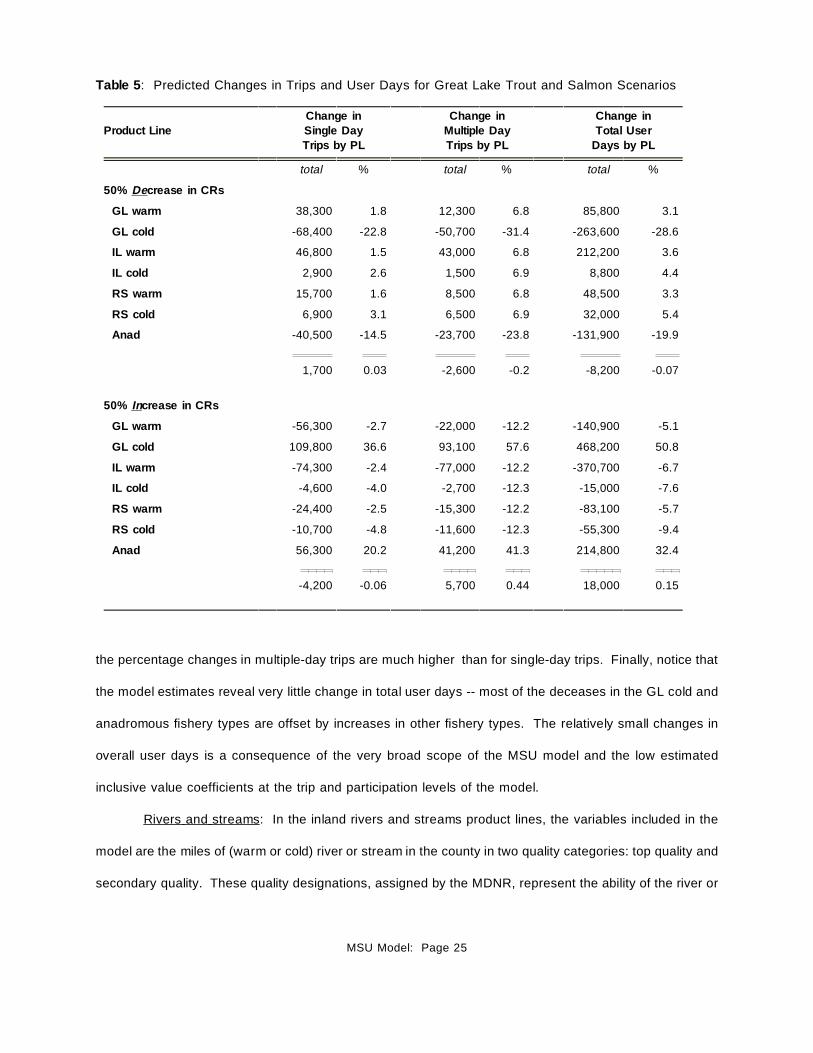
the percentage changes in multiple-day trips are much higher than for single-day trips. Finally, notice that

Table 5 : Predicted Changes in Trips and User Days for Great Lake Trout and Salmon Scenarios

Product LineChange inSingle DayTrips by PL

Change inMultiple DayTrips by PL

Change inTotal User

Days by PL

total % total % total %

50% Decrease in CRs

GL warm 38,300 1.8 12,300 6.8 85,800 3.1

GL cold -68,400 -22.8 -50,700 -31.4 -263,600 -28.6

IL warm 46,800 1.5 43,000 6.8 212,200 3.6

IL cold 2,900 2.6 1,500 6.9 8,800 4.4

RS warm 15,700 1.6 8,500 6.8 48,500 3.3

RS cold 6,900 3.1 6,500 6.9 32,000 5.4

Anad -40,500 -14.5 -23,700 -23.8 -131,900 -19.9

1,700

0.03

-2,600

-0.2

-8,200

-0.07

50% Increase in CRs

GL warm -56,300 -2.7 -22,000 -12.2 -140,900 -5.1

GL cold 109,800 36.6 93,100 57.6 468,200 50.8

IL warm -74,300 -2.4 -77,000 -12.2 -370,700 -6.7

IL cold -4,600 -4.0 -2,700 -12.3 -15,000 -7.6

RS warm -24,400 -2.5 -15,300 -12.2 -83,100 -5.7

RS cold -10,700 -4.8 -11,600 -12.3 -55,300 -9.4

Anad 56,300 20.2 41,200 41.3 214,800 32.4

-4,200

-0.06

5,700

0.44

18,000

0.15

the model estimates reveal very little change in total user days -- most of the deceases in the GL cold and

anadromous fishery types are offset by increases in other fishery types. The relatively small changes in

overall user days is a consequence of the very broad scope of the MSU model and the low estimated

inclusive value coefficients at the trip and participation levels of the model.

Rivers and streams: In the inland rivers and streams product lines, the variables included in the

model are the miles of (warm or cold) river or stream in the county in two quality categories: top quality and

secondary quality. These quality designations, assigned by the MDNR, represent the ability of the river or

MSU Model: Page 25

stream to support naturally-reproducing populations of relevant fish species. To provide an illustration of

Table 6 : Predicted Changes in Trips and User Days for Oakland County Stream Restoration.

Product LineChange in Single Day Trips by PL

Change in Multiple Day Trips by PL

Change in Total User

Days by PL †

total % total % total %

GL warm -18,400 -0.9 % -400 -0.2 % -19,920 -0.7 %

GL cold -1560 -0.5 % -340 -0.2 % -2,850 -0.3 %

IL warm -29,800 -1.0 % -1,430 -0.2 % -35,290 -0.6 %

IL cold -580 -0.5 % -50 -0.2 % -770 -0.4 %

RS warm 53,330 5.5 % 2,310 1.9 % 62,210 4.3 %

RS cold -1,160 -0.5 % -200 -0.2 % -1,930 -0.3 %

Anad -1,310

-0.5 % -190

-0.2 % -2,050

-0.3 %

Totals* 520 0.01 % -290 -0.02 % -600 ~0 %

a river restoration evaluation, consider a hypothetical policy that results in 100 miles of secondary quality

warm-water stream in Oakland County being improved to top quality. Oakland County is part of the Detroit

metropolitan area and is indicated on the map in Figure 3 by the asterisk. The analysis of a hypothetical

change of 100 miles of Oakland County secondary quality streams to top quality streams for one open

water season results in an estimated statewide benefit of about $730,000 dollars per year.

The changes in trips that result from the Oakland policy are presented in Table 6 (the format follows

that of Table 5). The results in Table 6 imply that there are slight increases in the total predicted single day

trips that are offset by slight decreases in the total predicted multiple day trips. However, as with the catch

rates scenarios, these changes are negligible. To provide a feel for the functioning of the model at the site

level, we now briefly explore the predicted changes in trips for specific counties in Michigan for the

hypothetical river restoration scenario.

Single day trips: As presented in Table 6, as a result of the hypothetical Oakland stream

improvement, predicted RS warm single-day trips increase by 53,000 (5.5%). Almost all of this increase

in trips is offset by decreases in other product lines. Over half the increase in RS warm single day trips

MSU Model: Page 26

is offset by decreased single-day trips from the IL warm

Figure 3: Single Day Trips UnderOakland Policy.

product line (a 1% decrease in IL warm). Most of the

remaining trips are drawn from the GL warm product line. The

model predicts that RS warm single day trips increase at

Oakland County by 61,300. From Table 6 it is clear that most

of these trips are drawn from other product lines (53,300 of

them), though 8,000 trips are drawn from other sites within the

RS warm product line.

Figure 3 depicts the changes in the pattern of single

day trips. The upper map shows the decreases in single-day

trips that occur within the RS warm product line at sites other

than Oakland. The lower map presents the county level

changes in the combined single-day trips for all product lines

other than RS warm. From Figure 3, it is clear that most of

the predicted increase in RS warm single-day trips to Oakland

is offset by reductions of other types of single-day trips at

Oakland and the immediately adjacent counties. For example,

within the RS warm sites (top map), the counties bordering Oakland account for 72% of the 8,000 trips that

are lost to RS warm sites other than Oakland. For the 53,000 trips that are drawn from outside the RS

warm product line, Oakland experiences the largest losses -- 17,200 single-day trips across all other product

lines. Thus, of the 61,300 trip increase in RS warm single day trips to Oakland, 28% of them come from

single-day trips to other product lines at Oakland (activity substitution rather than site substitution). Almost

all of the other reductions in single-day trips outside the RS warm product line come from counties in the

vicinity of Oakland (see the lower diagram in Figure 3).

Multiple day trips: Inspection of Table 6 reveals that the Oakland policy results in an increase of

2,300 multiple day trips in the RS warm product line, an increase of about 2%. This increase is more than

MSU Model: Page 27

offset by reductions in multiple-day trips in other product lines.

Figure 4: Multiple Day Trips UnderOakland Policy.

As with single-day trips, most of the trips are drawn from the

IL warm and GL warm product lines.

The model predicts that RS warm multiple-day trips

increase at Oakland by 4,000. From Table 6, just over half of

these trips are drawn from other product lines, and 1,700 trips

are drawn from other sites within the RS warm product line.

Figure 4 depicts the changes in the pattern of multiple-day

trips. The upper figure shows the decreases in multiple-day

trips that occur at sites other than Oakland within the RS warm

product line. The lower figure presents the county level

changes in the combined multiple day trips for all product lines

other than RS warm.

For multiple-day trips in the RS warm product lines,

the five counties losing the most trips to Oakland account for

only 25% of the multiple-day trips that are drawn from other

RS warm counties, as contrasted with single-day trips where

the top five counties accounted for 65% of the trips that were lost within the RS warm product line. Clearly,

the multiple day trip changes are more diffuse than for single day trips.

That the impacts on multiple day trips are more spread out than for single-day trips is also true for

the changes in multiple-day trips outside the RS warm product line, as seen in the lower diagram of Figure

4. For the trips that are drawn from outside the RS warm product line, Oakland experiences the largest

losses -- 180 multiple-day trips across all product lines other than RS warm. Of the 4,000 additional

multiple-day trips to Oakland for RS warm, only 5% come from other product lines at Oakland. The five

counties that experience the largest reductions in multiple-day trips to all other product lines besides RS

warm account for only 20% of the multiple-day trips that are drawn from outside the RS warm product line,

MSU Model: Page 28

as contrasted with single-day trips where the top five counties accounted for 77% of the trips lost outside

the RS warm product line. Bear in mind that while the figures illustrate that the impacts on multiple-day

trips are much more diffuse, these changes in multiple-day trips are extremely small. In contrast, the

changes in multiple-day trips were substantial for the larger scale trout and salmon scenarios.

Additional River Scenarios: The 100 mile warm-water Figure 5 : Distribution of population andlocation of RSw policy counties

river restoration scenario that was applied to Oakland County

is also applied to five additional counties in Michigan. These

examples illustrate the role that factors such as site location,

distance from population centers, and the mix of single and

multiple day trips have on the policy scenarios. The five other

counties are: Berrien County, located in the southwestern

most corner of the state and bordering Lake Michigan;

Gladwin County, located near the middle of the Lower

Peninsula; Presque Isle County, located on the northern tip of

the Lower Penninsula and bordering Lake Huron; Mackinac County, located in the southeastern part of the

Upper Penninsula just over the bridge from the Lower Penninsula; and Ontonogon County, located in the

northwestern Upper Penninsula and bordering Lake Superior. The map of Michigan in Figure 5 depicts the

location of each of these counties. Also shown in Figure 5 is the distribution of Michigan's population.

Table 7 presents the results of a hypothetical change from second to top quality for 100 miles of

warm-water streams in each county. The first row shows the estimated annual dollars of use-value

associated with the scenario. The values range from $730,000 at Oakland to $83,000 dollars at Ontonogon.

This illustrates the expected effect that proximity to population centers has on use-values. The second set

of rows present the predicted single day trips, multiple day trips, and user days for RSw fishing at the

baseline levels of the stream data. Also shown is the percentage of trips that are single versus multiple

day at each county which plays a role in the value results. The third set of rows presents the predicted

changes in trips and user days following the restoration scenario.

MSU Model: Page 29

Looking across the counties (columns in Table 7), one sees the effect that multiple day trips have

Table 7: Comparison of Warm-Water River Restoration Scenario at Alternative Counties in Michigan

Results of 100 mile warm-water river restoration at six Michigan c ounties

Oakland Berrien Gladwin PresqueIsle Mackinac Ontonogon

Value of improving 100miles of warm river totop quality

$730,300 $710,500 $479,300 $233,900 $172,800 $82,900

Predicted RSw tripsper county

- single day 40,130 13,780 5,680 1,240 560 560

- multiple day 1,160 2,380 1,860 930 690 340

- % single day 97% 85% 75% 57% 45% 62%

- user days 44,600 22,950 12,850 4,830 3,210 1,870

Change in predictedRSw trips per county

- single day 61,320 17,740 8,620 1,790 850 780

- multiple day 3,990 8,160 5,700 3,230 2,510 1,080

- user days 76,660 49,180 30,540 14,240 10,510 4,930

User day value (value÷ change in user days) $9.53 $14.45 $15.69 $16.43 $16.44 $16.82

Value per trip(value ÷ change intotal trips)

$11.18 $27.43 $33.47 $46.59 $51.43 $44.57

on the value results. As one moves to the right in the table, the baseline user days fall off more rapidly

than the changes in the user days while the value estimates fall even less. This is generally due to the

increased share of trips changes that are due to multiple day trip as one moves to right in the table. For

example, compare the results for Oakland and Berrien where the value estimates are similar. Berrien is

father away and receives a smaller number of trips than Oakland. However, Berrien has a higher

percentage of multiple day trips and experiences a much larger change in multiple day trips (more than

double) while single day trip changes are less than one third that of Oakland. Recall that the estimation

MSU Model: Page 30

results suggest changes in quality are more valuable for multiple day trips than for single day trips.

Moreover, the share of trips at a site that are multiple day trips tends to increase for sites that are farther

from population centers. Thus, the value associated with multiple day trips tend to offset some of the

decline in value of environmental quality that is associated with increased distance from population centers.

User day values: A common practice in recreational demand analysis is to translate estimated

values for changes in environmental quality into user-day values by dividing by the estimated change in

user days. The final rows of Table 7 present estimates of the user day values and per trip values

associated with the warm-water river restoration at the various counties. Notice that the user-day values

are much more stable than the per trip values (also shown in Table 7). For the sake of comparison,

estimated user-day values for the Great Lakes trout and salmon catch rates scenarios presented earlier can

be found by dividing the total values by the change in Great Lake trout and salmon trips. This yields user

day values of $27 and $33 for the trout and salmon scenarios. These user-day value estimates for Great

Lake trout and salmon are in the middle to low end of the range of values (adjusted to 1994 dollars) for cold

water and anadromous fishing reported by Walsh et al, while the river value is at the very low end of the

values for warm-water fishing reported by Walsh et al. In comparing the estimated values, one might be

tempted to conclude that one would not have gone too far awry in a benefit transfer analysis by using the

user day values from the literature. Bear in mind that a literature summarizing user-day values is not

sufficient for a benefits transfer -- transferring user-day value estimates requires some estimate of how user

days change in response to some policy.

Note that a complication in calculating and comparing user day values from RUMs arises when

trying to determine the appropriate level of the model at which to calculate changes in user days. Many

of the user day value estimates in the literature (and used in benefits transfer) are derived from single site

models under site closure policies in which the estimate is formed by dividing the lost consumer surplus

for the site by the lost trips. In such cases, there is no ambiguity about what trip change to use as the

divisor. However, with RUM models with many sites and levels, the choice of trip change is less clear --

especially for policies affecting quality at multiple sites. Had the trip changes at the product line level been

MSU Model: Page 31

used to derive the user day values for the river scenarios reported in Table 7 they would be closer to (but

still lower than) the trout and salmon values. Specifically, the user-day values using the RSw level trip

changes would be $11.74 for Oakland, $20.50 Berrien, $23.49 for Gladwin, $26.22 for PresqueIsle, $27.58

for Mackinac, and $25.51 for Ontonogon.

Conclusions

The purpose of this paper was to provide a summary of the development and estimation of the

Michigan RUM. While it is not the first repeated nested-logit model of recreation demand, the model is

novel in its size and breadth. The model involved 1,900 anglers, each with over 60 choice occasions and

with the average choice set on each occasion containing about 600 feasible alternatives. The use of the

repeated nested-logit framework allowed us to incorporate site quality characteristics and choice sets that

varied over time for each individual. In addition to the usual practice of differentiating choices by location,

trips were distinguished by duration, water body fished at, and species sought. The combined geographic

scale and broad range of trips types contained in the model makes the research unique. The extent of the

model is a reflection of the abundant and complex array of water and fishery resources in Michigan.

From the hypothetical policy simulations, we saw that site substitution and activity substitution

mattered for all the policies examined. In particular, the Michigan model exhibits a significant degree of

substitution among the different water bodies and specie types. As expected, the larger the scale of the

policy (as in the catch rates scenarios), the larger the amount of substitution in and out of the alternative

fishery types. However, even with the single site river restoration policy, the model indicated a large share

of the increase in trips to the county where restoration occurred were drawn from other fishery types in the

same county. Moreover, capturing the substitution possibilities for multiple-day trips requires a large model

scope, and the results indicated that with for the larger scale catch rate policies, the changes in multiple-day

trips were substantial. These findings are especially notable in light of the fact that most angling demand

models in the literature are restricted to a subset of the site types (e.g., inland lakes), fishing types (e.g.,

salmon), or trip lengths.

MSU Model: Page 32

Another important finding was that the results indicate limited substitution among trip lengths and

negligible changes in the overall number of predicted fishing trips, even for the very large scale catch rate

changes at the Great Lakes. While aggregate trips changes tend not to get reported, there is some

evidence that many recreational demand models in which site choices are based on RUM-type frameworks

are inelastic at the aggregate trip level. That is, demands for individuals sites are elastic, but the total trip

demands are very inelastic to changes in site quality. Whether this is a feature of the RUM modeling

approach or a more general characterization of recreational angling is an important area for future research.

Finally, we cannot underestimate the importance of the trip counts collected through the survey.

Since intervening events and longer time periods adversely affect anglers' ability to accurately recall the

number of fishing trips they have taken over some time interval, these factors need to accounted for during

the design of the surveys used to collect behavioral information. While the accuracy of the recalled number

of trips may have little impact on the site and activity portions of such a model, they will directly affect the

estimated aggregate number of trips and the aggregate values. We note that there are many examples

in the literature of the differences that model specification strategies may have on sample values, yet the

process of extrapolating results to more general populations is often ignored. Of course, it is the aggregate

values that serve as the basis for water resource management decisions.

A few words of caution are in order in regards to interpreting the valuation results. First, since the

estimated values are based on the travel cost method, they are only estimates of use-value. Second, the

results only apply to Michigan anglers who fish in Michigan. There are many non-resident anglers who fish

in Michigan whose values are not accounted for. Third, the trips that are included in the MSU model are

only those trips where anglers indicated that fishing was the primary purpose of the trip. The survey results

indicated that fishing was the primary purpose for 97% of the single day trips and for 67% multiple day trips.

In sum, there are a fair amount of trips that involve fishing (and hence, user days and value) that are

outside realm of the MSU model. Finally, while the results presented here represent our best efforts to

date, our research and the development of the MSU model is on-going.

MSU Model: Page 33

References

American Automobile Association, Your Driving Costs, 1993.

Ben-Akiva, Moshe, and Steven R. Lerman, Discrete Choice Analysis: Theory and Application to TravelDemand, Cambridge: MIT Press, 1985.

Bence, J.R., and K.D. Smith, "An Overview of Recreational Fisheries of the Great Lakes," in Great LakesFisheries Policy and Management: a Binational Perspective (W.W. Taylor and P. Fererri eds.) EastLansing: Michigan State University Press, forthcoming.

Bockstael, Nancy E., W. M. Hanemann, and I. E. Strand, "Measuring the Benefits of Water QualityImprovements Using Recreation Demand Models," EPA Contract No. CR-811043-01-0, 1984.

Bockstael, Nancy E., W. Michael Hanemann, and Catherine L. Kling, "Estimating the Value of Water QualityImprovements in a Recreational Demand Framework," Water Resources Research, 23(5):951-960,May, 1987.

Freeman III, A. Myrick, The Measurement of Environmental and Resource Values: Theory and Methods,Washington, D.C.: Resources for the Future, 1993.

Greene, William H., Econometric Analysis, New York: MacMillan Publishing Co., 1993.

Greene, William H., Limdep Version 6.0 User's Manual and Reference Guide, Econometric Software, 1992.

Herriges, Joseph A., and Catherine L. Kling, "Testing the Consistency of Nested Logit Models with UtilityMaximization," Economic Letters, 50(1):33-39, January, 1996.

Hoehn, John P., Theodore Tomasi, Frank Lupi, and Heng Z. Chen, An Economic Model for ValuingRecreational Angling Resources In Michigan, Report submitted to the Michigan Department of NaturalResources and the Michigan Department Environmental Quality, December, 1996.

Johnson, N., and S. Kotz, Discrete Distributions, New York: Wiley and Sons, 1969.

Jones, Carol Adair, and Yusen D. Sung, Valuation of Environmental Quality at Michigan Recreational Sites:Methodological Issues and Policy Applications, Final Report, EPA Contract No. CR-816247-01-2,September, 1993.

Kikuchi, Hideo, Segmenting Michigan's Sport Fishing Market: Evaluation of Two Approaches, PhDDissertation, Michigan State University, 1986.

Kmenta, Jan, Elements of Econometrics, New York: MacMillan Publishing Co., 1986.

Mahoney, Edward M., Douglas B. Jester, Jr., Gale C. Jamsen, "Chapter 16- Recreational Fishing in Michigan,"in: Travel and Tourism in Michigan: A Statistical Profile, (Dan Spotts, ed.), Travel, Tourism, andRecreational Resource Center, Michigan State University, 307-343, 1991.

McFadden, Daniel, "Computing Willingness-To-Pay in Random Utility Models," Resources and Energy,forthcoming 1998.

McFadden, Daniel, "Econometric Models of Probabilistic Choice Models," in: Structural Analysis of DiscreteData with Applications, (Manski, Charles, and Daniel McFadden, eds.), Cambridge: MIT Press, 1981.

MSU Model: Page 34

Merna, James W., James C. Schneider, Gaylord R. Alexander, Warren D. Alward, and Randy L. Eshenroder,Manual of Fisheries Survey Methods, Fisheries Management Report No. 9, Fisheries Division,Michigan Department of natural Resources, 1981.

Morey, Edward R., TWO RUMs un CLOAKED: Nested-Logit Models of Site Choice and Nested-Logit Modelsof Participation and Site Choice, Western Regional Project W-133, 7th Interim Report, June, 1994.

Morey, Edward R., Robert D. Rowe, Michael Watson, "A Repeated Nested Logit Model of Atlantic SalmonFishing," American Journal of Agricultural Economics, 75(3):578-592, August, 1993.

Train, Kenneth, Qualitative Choice Analysis, London, England, 1986.

Walsh, R. G., D. M. Johnson, and J. R. McKean, "Benefit Transfer of Outdoor Recreation Demand Studies,1968-1988," Water Resources Research, 28(3):707-713, 1992.

WESTAT, Inc., Investigation of Possible Recall/Reference Period Bias in National Surveys of Fishing, Hunting,and Wildlife-Associated Recreation, U.S. Department of the Interior, Washington, D.C., 1989.

Appendix

The MSU model of the demand for recreational fishing in Michigan is a repeated random utility model

estimated as a four-level nested logit. The general structure (i.e., trip types, choice sets, choice occasions,

nesting, etc.) was presented in the text. This appendix provides the exact model specification. On a given

occasion, let Ukstp be the indirect utility of taking a trip to county k, product line/shoreline s, and trip length t,

given a trip is taken (participation) p. Let Uh be the utility of not fishing, where h indicates not fishing. Under

the hypothesis of utility maximization, the decision on any occasion of fishing and taking the trip to a particular

county kd, shore line and product line sd, at length td imply the utility inequality:

for all feasible {k,s,t}≠{kd,sd,td }, i.e., the utility of the chosen site and trip type is greater than the utility of any

(A.1)Ukdsdtdp > Ukstp and Ukdsdtdp > Uh

other type of trip to any other site in the choice set. Similarly, if the "not fishing" is observed on the occasion,

we have the inequality Uh > Ukstp for all feasible {k,s,t}.

Since all the factors that influence the individuals' choices cannot be observed, the utility function Ukstp

is treated as stochastic and specified as the sum of a deterministic term, Vkstp , and a stochastic term, εkstp.

Vkstp is the deterministic indirect utility of taking a trip of type kst, which we specify as a linear function of

MSU Model: Page 35

explanatory variables and parameters to be estimated. The "not fishing" utility is given by Uh = Vh +εh where

Vh is a function of demographic variables. The ε's represent the stochastic utility terms that are not measured

by researchers and are assumed to follow a generalized extreme value (GEV) distribution. Repeating the

utility maximization behavior over the occasions in a season results in a repeated-logit model.

The Likelihood Function and Choice Probabilities: On an occasion in month m, let Pr imkstp be the joint

choice probability of taking a trip to county k in product line/shoreline combination s of trip length t for individual

i during month m. Let Pr imh be the probability of not taking a trip on the occasion in month m. For individual

i, the likelihood function during month m is the product of the joint choice probabilities Pr imkstp for the occasions

in which the trips are observed and the probabilities Pr imh for the occasions when there are no trips. That is

L im = NOCim×Pr im

h × { ∏ Pr imkstp } (A.2)

kst∈Im

where NOCim is the number of choice occasions in month m where no trip is observed, and Im is the set of

sites/trip types (kst) for individual i during month m. As a result, the product of the Lim over all individuals

and months yields the sample likelihood function, L =∏im Lim.

To estimate the nested-logit model by maximizing the likelihood function L, the choice probability

of taking a trip on an occasion in month m for individual i (Pr imkstp ) can be re-expressed as the product of

the conditional probabilities as follows (the superscript i is suppressed in what follows):

Pr mkstp = Pr m

kstp Pr mstp Pr m

tp Pr mp (A.3)

where the conditional probabilities in the right hand side of the equation are defined as follows:

Pr mkstp the probability of a trip to county k in month m, conditional on product line/shoreline

combination s, trip length t, and participation p.

Pr mstp the probability of a trip to product line/shoreline combination s in month m, conditional on

a trip of length t, and participation p.

Pr mtp the probability of a trip of length t in month m, conditional on participation p.

Pr mp the probability of taking a trip on a choice occasion in month m.

MSU Model: Page 36

The random terms were assumed be jointly distributed according to the following generalized

extreme value (GEV) distribution

where the subscripts k, s, t, p index the feasible counties, product line/shoreline combinations, trip lengths,

(A.4)

and the participation, respectively. The k, s, t, p subscripts index groups of alternatives within the four-level

hierarchy of the nesting structure (see McFadden 1981 for more on the GEV distribution). To increase the

model's flexibility, there are separate scale parameters at the level of the product line/shoreline

combinations (ρt ) for the single-day trip branch and the multiple-day trip branch. The other scale

parameters ω and η remain the same within their respective levels.

Conditional Choice Probabilities: At the bottom level of the nested-logit, the conditional probability

of taking a trip to county k in product line/shoreline combination s of length t in month m is

where kstp means that the summation is over the feasible counties within the product line/shoreline

(A.5)Prkstp exp(αt1pkt αt

2qmks αt

3Cbnkt)

kstpexp(αt

1pkt αt2q

mks αt

3Cbnkt)

combination s, trip length t, and participation p in month m. α represents parameters to be estimated.

There are three types of explanatory variables at this level: (i) pkt are the individual specific travel costs;

(ii) qksm are the site quality variables, and the superscript m reflects the monthly catch rates; and (iii) Cbnkt

is a dummy for individuals with a cabin in county k. The t superscript on α reflects the fact that separate

parameter vectors were used to index single and multiple-day trips (α1 and α2, respectively), allowing the

variables to have different effects on the utility of trips of different length. The inclusive value of taking a

trip to product line/shoreline s of length t in month m is ivmstp = log[ kstp exp (α1

t qksm +α2

t pkt+α3t Cbnkt )].

On the third level, the conditional probability of taking a trip to the product line/shoreline s of length

t in month m is:

MSU Model: Page 37

where stp indicates summation over all feasible product line/shoreline combinations s∈S. There are two

(A.6)Prstp exp(β t1iv

imstp β t

2Ds)

stpexp(β t

1ivimstp β t

2Ds)

types of explanatory variables at this level: (i) Eleven dummy variables (Ds ) for the combinations of

product lines and counties with/without GL shoreline, s. GLwarm is normalized at 0 for identification during

the model estimation; and (ii) The inclusive values ivmstp of taking a trip to s, calculated from the bottom level.

βt is the vector of parameters to be estimated. The t superscript reflects the fact that the parameter vectors

differ by the trip lengths: β1 is for single-day trips and β2 is for multiple-day trips (β2). Then, the inclusive

value of taking a trip of length t in month m is: ivmtp = log [ stpexp(βt

1 ivmstp +βt

2Ds )].

At the second level, the conditional probability of taking a trip of length t in month m is:

where tp means that the summation is over the single-day and multiple-day trip types, given participation.

(A.7)Prtp exp(γ 1ivmtp γ 2Dt γ 3Tct Jb)

tpexp(γ 1iv

mtp γ 2Dt γ 3Tct Jb)

The conditional trip length probability has three variable types: (i) A dummy with Dt=1, if it is a multiple-day

trip, 0 otherwise; (ii) The trip's time cost interacted with a dummy for individuals without a job (Tct×Jb); and,

(iii) The inclusive values ivmtp calculated from the shoreline/product line level.

At the top level, the probability of taking a trip in month m is

where δ are the parameters to be estimated. In any month m, there are two types of variables at the

(A.8)Prp exp(δ 1ivmp δ 3Dm)

exp(δ 2sd) exp(δ 1ivmp δ 3Dm)

participation level: (i) seven dummy variables; Dm=1 if the trip was observed in month m for April through

October, and (ii) the inclusive values ivmp calculated from the trip length choice level. Similarly, the

probability of not fishing on an occasion in month m is

MSU Model: Page 38

Again, δ are the parameters to be estimated. The relative utility of not fishing is indexed by three

(A.9)Prh exp(δ 2sd)

exp(δ 2sd) exp(δ 1ivmp δ 3Dm)

demographic variables sd: (1) the natural logarithm of age, (2) the natural logarithm of years of education,

and (3) gender with 1 for male, 0 for female.

Welfare Measurement: The MSU model can be used to estimate the benefits attributable to site

quality changes and to the addition or elimination of a site. The welfare measures are calculated as the

areas under the site demand curves conditional on the number of single and multiple day trips. The overall

welfare measure is then the sum of the trip weighted welfare measures. Specifically, for each individual,

we calculate a monthly welfare measure and then sum these across individuals and across months. The

welfare measure for individual i (with the i superscript suppressed) is defined by

W = m (TmSD×CVm

SD + TmMD×CVm

MD ) (A.10)

where Tmt is the predicted single day (multiple day) trips in month m for this individual and CVm

t is the

individual's welfare measure conditional on a trip of length t in month m. Tt is given by Ocm×Prmt|p×Prm

p where

t=sd,md; Ocm is the feasible number of occasions in month m; and Prmt|p×Prm

p is the probability of taking a

trip of length t in month m as defined above. CVmt is given by {ivm

tp(1)-iv mtp(0)}/λt where 0,1 refer to the "with"

and "without" levels of quality; ivmtp is the inclusive value of taking a trip of length t in month m as defined

above; and λt equals -α1t×β1

t for t=sd,md where -α1t×β1

t recovers the underlying parameter on travel costs

for single and multiple day trips. The individual welfare measures are then weighted using the survey

weights for complete panel data, and the weighted average is then expanded to the population of potential

anglers in Michigan as estimated from the screening interview.

MSU Model: Page 39