the measurement of overhead conductor’sag with dlt method

Copyright © 2017, the Authors. Published by Atlantis Press.This is an open access article under the CC BY-NC license (http://creativecommons.org/licenses/by-nc/4.0/).

The measurement of overhead conductor’s sag

with DLT method

Fang Ye1†, Meng Tian2, Xing Zhang2,

Zhi-Yong Gan3, Xin He3 and Zhang-Qi Wang2

1Electric Power Research Institute, State Grid Tianjin

Electric Power Company, Tianjin, 300384, China

E-mail: [email protected] 2Department of Mechanical Engineering, North China

Electric Power University, Baoding, 071003, China 3Electric power science and Technology Development Co.,

Ltd. of Tianjin city, Tianjin 300384, China

The overhead conductor sag calculation is put forward combined with image analysis

technology based on DLT theory in this paper. Moreover, the simulation experiment is

carried on and the measurement error is also analyzed. The attentions needed in practical

operation are also provided. The result shows that the method provided in this paper is a

quick, efficient and practical measurement method for transmission line inspection.

Keywords: Direct Linear Transformation; Overhead Conductor; Sag.

1. Introduction

The electric power system is the foundation of China's economic construction,

and it is also an important guarantee for the national life. Sag is one of the

important parameters for operation and maintenance of transmission lines, so it is

necessary to control the sag of overhead conductor within the allowable range. If

the sag is too small, the wire stress will be increased, which will cause more

vibration and the break of transmission line, and even the damage of electric

power tower. If the sag is too large, the safe distance between the wire and the

ground is not enough, and the discharge phenomenon will be taken place, and

even the phenomenon of short twist is occurred to conductor galloping. And

furthermore, sag is one of the limiting factors to increase the transmission capacity

of overhead transmission lines. The transmission capacity can be adjusted by the

real-time dynamic measurement of the sag, which could release the conservative

transmission capacity to achieve the purpose of dynamic capacity increase [1].

Therefore, it is of great significance to measure the sag of overhead transmission

lines regularly to ensure the safe operation of the whole power grid.

The traditional methods of sag measurement include angle method, equal

365

2nd Annual International Conference on Electronics, Electrical Engineering and Information Science (EEEIS 2016)Advances in Engineering Research (AER), volume 117

length method and relaxation plate observation method, etc, but these methods are

very inconvenient to operate, and have large human error and low measurement

efficiency. In reference [2], the local meteorology parameters are considered as

the control condition, and the wire sag is calculated by measuring the stress or

inclination of conductor in combination with the conductor state equation, but this

method requires a large investment and has high cost. Chris Menasha Bonus in [3]

studies DGPS technology for conductor sag measurement. This method uses four

satellites to locate the position of Rover that can be used in any environment

hanging fixed point for overhead conductor sag measurement, however, the price

of this measurement method is very expensive, and the power consumption is also

high. The reference [4] shows that the spacer is used as a template to match the

spacer of the conductor through image processing, then three-dimensional

coordinate transformation is carried out for the match point, the conductor sag is

calculated by curve fitting of world coordinates of the match point. As the spacer

could be out of shape in different positions and is easily affected by the environ-

ment during the matching procedure, it is also difficult to measure transmission

lines sag in practical application.

In this paper, a new method is put forward to measure the overhead conductor

sag based on two-dimensional plane image analysis. In the present method, a

marker on the measuring spot is used and the coordinates of the marked point is

obtained by a photograph analysis method.

2. Director Linear Transformation

2.1. Camera imaging model

The camera imaging model is an important part of the measurement system. In

the monocular vision, according to requirements of the measurement and the

actual situation, the camera imaging model can be divided into vertical projection

model, weak perspective imaging model, pinhole imaging model, and so on.

Among of them, the pinhole imaging model is the closest to the actual situation

[5-7]. So this paper selects the pinhole model as camera imaging model.

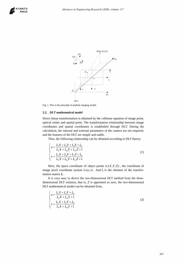
The principle of pinhole imaging model is shown in the Fig.1. Spatial point

P passes through the optical center O, and PO intersect at p point with in the

projection plane.

The camera coordinate of spatial point P is denoted as , ,C C CX Y Z , the space

coordinate of space coordinates system w W w wO X Y Z is , ,P X Y Z , corres-

ponding to the image pixel coordinate of the projection point p ( , )u v .

366

Advances in Engineering Research (AER), volume 117

P

y

x

Xc

Yc

O

o

Zc

Xw

Zw

Yw

Ow

P(Xc,Yc,Zc)

u

v

Fig. 1. This is the principle of pinhole imaging model.

2.2. DLT mathematical model

Direct linear transformation is obtained by the collinear equation of image point,

optical center and spatial point. The transformation relationship between image

coordinates and spatial coordinates is established through DLT. During the

calculation, the internal and external parameters of the camera are not required,

and the features of the DLT are simple and stable.

Thus, the following relationship can be obtained according to DLT theory:

1 2 3 4

9 10 11

5 6 7 8

9 10 11

1

1

L X L Y L Z Lu

L X L Y L Z

L X L Y L Z Lv

L X L Y L Z

(1)

Here, the space coordinate of object points is ( , , )X Y Z , the coordinate of

image pixel coordinate system is ( , )u v . And iL is the element of the transfor-

mation matrix L .

It is very easy to derive the two-dimensional DLT method from the three-

dimensional DLT solution, that is, Z is appointed as zero, the two-dimensional

DLT mathematical model can be obtained from,

1 2 4

9 10

5 6 8

9 10

1

1

L X L Y Lu

L X L Y

L X L Y Lv

L X L Y

(2)

367


Note that there are only 8 variables in the two-dimensional DLT mathematical

model, while the 3D DLT mathematical model has 11 variables, so the two-

dimensional DLT has the advantages of small amount of calibration points, simple

operation and less computation. From the two-dimensional DLT model, if the

coordinates of 4 points in pace scene and their corresponding pixel coordinates

are available, 8 equations can be obtained and the transformation matrix L can be

known by solving these 8 equations.

3. Object Spatial Coordinates Calculation

In the calculation of the coordinates of spatial point, the transform matrix L should

be calculated first, then the object coordinates can be obtained by L , finally, the

conductor sag can be obtained by fitting the object coordinates.

3.1. Resolution of transformation matrix

When the spatial coordinates of n landmarks and corresponding pixel coordinates

are available, 2×n equations can be obtained as in following,

1 1 1 1 11 1

1 1 1 1 1 1 1

0 01 0

0 0 0 1

0 01 0

0 0 0 1

n n n n nn n

n n n n n n n

u X u Y uX Y

X Y X v v Y v

u X u Y uX Y

X Y X v v Y v

L (3)

where

1 2 4 5 6 8 9 10

TL L L L L L L LL

Then, the transform matrix is

1 1 1 1 11 1

1 1 1 1 1 1 11

0 01 0

0 0 0 1

,

0 01 0

0 0 0 1

T T

n n n n nn n

n n n n n n n

u u X u YX Y

v X Y X v v Y

u u X u YX Y

v X Y X v v Y

L A A A A (4)

In order to calculate the 8 variables of the transformation matrix L , the spatial

coordinates of at least 4 marker points and the corresponding pixel coordinates

should be known.

3.2. Calculation of object point coordinate

When the transformation matrix and the spatial coordinates of n landmarks and

the corresponding pixel coordinates are known, the spatial coordinates of the

368


object can be calculated according to,

1 4 1 1 9 2 1 101

1 8 5 1 9 6 1 1011

4 1 9 2 10

8 5 9 6 10

,T T

n n n n

n n n n

u L L u L L u LX

v L L v L L v LY

X u L L u L L u L

Y v L L v L L v L

B B B B (5)

3.3. Overhead line curve fitting

The two-dimensional spatial coordinates of each point of the overhead conductor

can be obtained by the Eq. (5), and then the calculation model of the conductor

can be calculated by the method of data regression.

The calculation model of overhead conductor can be described as catenary or

parabolic equation [8]. In order to avoid the hyperbolic function and simplify the

calculation, this paper adopts parabolic equation. The quadratic parabolic equa-

tion model of overhead conductor is shown as

2

0 1 2y k k x k x (6)

Here, ,x y is the spatial coordinate of a point on the overhead line, and0k ,

1k , 2k are undetermined coefficients. Using the nonlinear regression algorithm of

least square to fit the feature points of the conductor, the value of the undeter-

mined coefficients can be calculated, and then the sag of overhead conductor also

can be obtained easily.

4. Simulation Experiment Research

In order to verify the accuracy and feasibility of the overhead line sag calculation

method, the simulation experiment is carried on. For convenience, the height

between the ground and the conductor near stadia rod is taken as the measuring

object. In addition, the influence of distribution of the identification points on the

measurement accuracy has also been analyzed.

Since the smooth cable, with the characteristics of uniform load, inexten-

sibility and fully flexibility, is accord with the state of overhead line, it is used to

carry on the experiment instead of overhead line. The experimental image is

shown in Fig.2. The simulation conductor of this experiment is a constant height

suspension, and the related parameters are measured by the stadia rod. The ground

clearance of conductor is 200cm, and the side length value of checkerboard is 5cm

square.

369


Fig. 2. This is the simulation of experimental based on DLT.

If the checkerboard is placed in the conductor plane, the spatial coordinate of

each point of the conductor can be calculated according to the DLT theory. The

flowchart of the procedure is presented in Fig. 3.

Layout

identification point

Image

acquisition

The computation of

projection matrix

Conductor spatial

coordinte calculation

Fig. 3.This is the flow chart of the experimental procedure.

First, the calibration points on the checkerboard is chosen and the transfor-

mation matrix L is calculated according to the Eq. (4). Then, the measurement

point in the conductor is selected, and the two-dimensional spatial coordinates is

calculated according to the Eq. (5). In the experiment, the calibration points of

different distribution forms are selected and divided into six groups, that is, A1-

A4, B1-B4, C1-C4, D1-D4, E1-E4, F1-F4, respectively corresponding 1×1, 2×2,

4×4, 6×6, 8×8, 10×10 square. The distribution of calibration points are shown in

Fig. 4:

Fig. 4. This is the distribution of calibration points on the checkerboard

The actual value of the distance between conductor and ground is 200 cm,

while the calculation results of the identification points with different distribution

370


conditions are shown in table 1.

Table 1. This is the experimental result and the measurement error.

Size of calibration grid 1×1 2×2 4×4 6×6 8×8 10×10

Measured value(cm) 141.23 166.50 185.88 186.87 196.51 197.82

Relative error( ) 29.38% 16.75% 7.07% 6.57% 1.60% 1.09%

From the above results, it shows that the larger the surrounded area of

calibration points in the image proportion is, the smaller the measurement error is.

Moreover, the measured values are less than the actual value, which means there

are some system errors.

5. Conclusions

A measurement method for overhead conductor sag is put forward using two-

dimensional image measurement based on the DLT theory. The influence of the

distribution of the calibration points on the measuring accuracy is analyzed, which

shows the measurement accuracy is higher when the identification point is larger

than 1/4 in the image. The proposed method can calculate the conductor sag with

the characteristics of simple operation, good accuracy, high efficiency and practic-

ability, which avoids the disadvantages of the traditional manual measurement

method.

References

1. Forbes, Blake, D. Bradshow, and F. Campbell, Finding hidden capacity in

transmission lines. Transmission & Distribution World, 2002, 54, (9).

2. Wei Kong, Xiao-Guang Dai, Zhen-Wei Yang , Matlab realization of stress sag

curve of overhead line. Electric Power, 2009, 42 (7): 46-49.

3. Mensah-Bonsu C, Krekeler U F, Heydt G T, etc, Application of the global

positioning system to the measurement of overhead power transmission

conductor sag. IEEE Transactions on Power Delivery, 2002, 17(1):273-278.

4. Wei-Guo Tong, Bao-Shu Li, Jin-Sha Yuan, etc. Method of transmission line

sag measurement based on aerial image sequence. Proceedings of the CSEE,

2011, 16:115-120.

5. D.A.Forsyth, J.Ponce. Forsyth. Computer Vision: A Modern Approach.

Prentice Hall Professional Technical Reference, 2002.

6. R. Szeliski, Richard. Computer Vision: Algorithms and Applications. Journal

of Polymer Science Polymer Chemistry Edition 21.8 (2011):2601-2605.

7. M.S.Nixon, A.S.Aguado. Feature extraction and image processing. Beijing:

Electronic Industry Publishing House, 2011:288-308.

8. Dian-Sheng Zhang. Design Manual of High Voltage Transmission Line in

Power Engineering. Beijing: China Power Press, 2003.

371


the measurement of overhead conductor’sag with dlt method

Documents