the mcgraw-hill series
TRANSCRIPT


The McGraw-Hill Series Economics
ESSENTIALS OF ECONOMICS
Brue, McConnell, and FlynnEssentials of EconomicsSecond Edition
MandelEconomics: The BasicsFirst Edition
SchillerEssentials of EconomicsSeventh Edition
PRINCIPLES OF ECONOMICS
ColanderEconomics, Microeconomics,and MacroeconomicsSeventh Edition
Frank and BernankePrinciples of Economics,Principles of Microeconomics,Principles of MacroeconomicsFourth Edition
Frank and BernankeBrief Editions: Principles ofEconomics, Principles ofMicroeconomics, Principles ofMacroeconomicsFirst Edition
McConnell, Brue, and FlynnEconomics, Microeconomics,and MacroeconomicsEighteenth Edition
McConnell, Brue, and FlynnBrief Editions: Economics,Microeconomics,MacroeconomicsFirst Edition
MillerPrinciples of MicroeconomicsFirst Edition
Samuelson and NordhausEconomics, Microeconomics,and MacroeconomicsEighteenth Edition
SchillerThe Economy Today, The MicroEconomy Today, and The MacroEconomy TodayEleventh Edition
SlavinEconomics, Microeconomics,and MacroeconomicsNinth Edition
ECONOMICS OF SOCIAL ISSUES
GuellIssues in Economics TodayFourth Edition
Sharp, Register, and GrimesEconomics of Social IssuesEighteenth Edition
ECONOMETRICS
Gujarati and PorterBasic Econometrics Fifth Edition
Gujarati and PorterEssentials of Econometrics Fourth Edition
MANAGERIAL ECONOMICS
BayeManagerial Economics and BusinessStrategySixth Edition
Brickley, Smith, and ZimmermanManagerial Economics andOrganizational ArchitectureFifth Edition
Thomas and MauriceManagerial EconomicsNinth Edition
INTERMEDIATE ECONOMICS
Bernheim and WhinstonMicroeconomicsFirst Edition
Dornbusch, Fischer, and StartzMacroeconomicsTenth Edition
FrankMicroeconomics and BehaviorSeventh Edition
ADVANCED ECONOMICS
RomerAdvanced MacroeconomicsThird Edition
MONEY AND BANKING
CecchettiMoney, Banking, and FinancialMarketsSecond Edition
URBAN ECONOMICS
O’SullivanUrban EconomicsSeventh Edition
LABOR ECONOMICS
BorjasLabor EconomicsFourth Edition
McConnell, Brue, and MacphersonContemporary Labor EconomicsEighth Edition
PUBLIC FINANCE
Rosen and GayerPublic FinanceEighth Edition
SeidmanPublic FinanceFirst Edition
ENVIRONMENTAL ECONOMICS
Field and FieldEnvironmental Economics:An IntroductionFifth Edition
INTERNATIONAL ECONOMICS
Appleyard, Field, and CobbInternational EconomicsSixth Edition
King and KingInternational Economics,Globalization, and Policy: A ReaderFifth Edition
PugelInternational EconomicsFourteenth Edition
guj75772_IFC.qxd 01/08/2008 10:06 AM Page 2

Basic Econometrics
Fifth Edition
Damodar N. GujaratiProfessor Emeritus of Economics,United States Military Academy, West Point
Dawn C. PorterUniversity of Southern California
Boston Burr Ridge, IL Dubuque, IA New York San Francisco St. LouisBangkok Bogotá Caracas Kuala Lumpur Lisbon London Madrid Mexico CityMilan Montreal New Delhi Santiago Seoul Singapore Sydney Taipei Toronto
guj75772_fm.qxd 05/09/2008 11:15 AM Page i

BASIC ECONOMETRICS
Published by McGraw-Hill/Irwin, a business unit of The McGraw-Hill Companies, Inc., 1221 Avenue of theAmericas, New York, NY, 10020. Copyright © 2009, 2003, 1995, 1988, 1978 by The McGraw-Hill Companies,Inc. All rights reserved. No part of this publication may be reproduced or distributed in any form or by anymeans, or stored in a database or retrieval system, without the prior written consent of The McGraw-HillCompanies, Inc., including, but not limited to, in any network or other electronic storage or transmission, orbroadcast for distance learning.
Some ancillaries, including electronic and print components, may not be available to customers outside theUnited States.
This book is printed on acid-free paper.
1 2 3 4 5 6 7 8 9 0 VNH/VNH 0 9 8
ISBN 978-0-07-337577-9MHID 0-07-337577-2
Publisher: Douglas ReinerDevelopmental editor: Anne E. HilbertEditorial coordinator: Noelle FoxAssociate marketing manager: Dean KarampelasLead Project manager: Christine A. VaughanFull-service project manager: Michael Ryder, ICC Macmillan Inc.Lead production supervisor: Carol A. BielskiDesign coordinator: Joanne MennemeierMedia project manager: Srikanth Potluri, Hurix Systems Pvt. Ltd.Cover design: Brittany SkwierczynskiTypeface: 10/12 TimesNewRomanPSCompositor: ICC Macmillan Inc.Printer: R. R. Donnelley
Library of Congress Cataloging-in-Publication Data
Gujarati, Damodar N.Basic econometrics / Damodar N. Gujarati, Dawn C. Porter. — 5th ed.
p. cm.Includes bibliographical references and index.ISBN-13: 978-0-07-337577-9 (alk. paper)ISBN-10: 0-07-337577-2 (alk. paper)1. Econometrics. I. Porter, Dawn C. II. Title.
HB139.G84 2009330.01�5195—dc22
2008035934
www.mhhe.com
guj75772_fm.qxd 05/09/2008 11:15 AM Page ii

About the AuthorsDamodar N. GujaratiAfter teaching for more than 25 years at the City University of New York and 17 years in theDepartment of Social Sciences, U.S. Military Academy at West Point, New York, Dr. Gujaratiis currently Professor Emeritus of economics at the Academy. Dr. Gujarati received hisM.Com. degree from the University of Bombay in 1960, his M.B.A. degree from theUniversity of Chicago in 1963, and his Ph.D. degree from the University of Chicago in 1965.Dr. Gujarati has published extensively in recognized national and international journals, suchas the Review of Economics and Statistics, the Economic Journal, the Journal of Financialand Quantitative Analysis, and the Journal of Business. Dr. Gujarati was a member of theBoard of Editors of the Journal of Quantitative Economics, the official journal of the IndianEconometric Society. Dr. Gujarati is also the author of Pensions and the New York City FiscalCrisis (the American Enterprise Institute, 1978), Government and Business (McGraw-Hill,1984), and Essentials of Econometrics (McGraw-Hill, 3d ed., 2006). Dr. Gujarati’s bookson econometrics have been translated into several languages.
Dr. Gujarati was a Visiting Professor at the University of Sheffield, U.K. (1970–1971), aVisiting Fulbright Professor to India (1981–1982), a Visiting Professor in the School ofManagement of the National University of Singapore (1985–1986), and a Visiting Professorof Econometrics, University of New South Wales, Australia (summer of 1988). Dr. Gujaratihas lectured extensively on micro- and macroeconomic topics in countries such asAustralia,China, Bangladesh, Germany, India, Israel, Mauritius, and the Republic of South Korea.
Dawn C. PorterDawn Porter has been an assistant professor in the Information and Operations Manage-ment Department at the Marshall School of Business of the University of SouthernCalifornia since the fall of 2006. She currently teaches both introductory undergraduateand MBA statistics in the business school. Prior to joining the faculty at USC, from2001–2006, Dawn was an assistant professor at the McDonough School of Business atGeorgetown University, and before that was a visiting professor in the psychology depart-ment at the Graduate School of Arts and Sciences at NYU. At NYU she taught a number ofadvanced statistical methods courses and was also an instructor at the Stern School ofBusiness. Her Ph.D. is from the Stern School in Statistics.
Dawn’s areas of research interest include categorical analysis, agreement measures,multivariate modeling, and applications to the field of psychology. Her current research ex-amines online auction models from a statistical perspective. She has presented her researchat the Joint Statistical Meetings, the Decision Sciences Institute meetings, the InternationalConference on Information Systems, several universities including the London School ofEconomics and NYU, and various e-commerce and statistics seminar series. Dawn is alsoa co-author on Essentials of Business Statistics, 2nd edition, McGraw-Hill Irwin, 2008.Outside of academics, Dawn has been employed as a statistical consultant for KPMG, Inc.She has also worked as a statistical consultant for many other major companies, includingGinnie Mae, Inc., Toys R Us Corporation, IBM, Cosmaire, Inc., and New York University(NYU) Medical Center.
iii
guj75772_fm.qxd 05/09/2008 11:15 AM Page iii

For Joan Gujarati, Diane Gujarati-Chesnut,
Charles Chesnut, and my grandchildren,
“Tommy” and Laura Chesnut.
—DNG
For Judy, Lee, Brett, Bryan, Amy, and Autumn Porter.
But especially for my adoring father, Terry.
—DCP
guj75772_fm.qxd 05/09/2008 11:15 AM Page iv

Brief ContentsPreface xviAcknowledgments xix
Introduction 1
PART ONESingle-Equation Regression Models 13
1 The Nature of Regression Analysis 15
2 Two-Variable Regression Analysis: Some Basic Ideas 34
3 Two-Variable Regression Model: TheProblem of Estimation 55
4 Classical Normal Linear RegressionModel (CNLRM) 97
5 Two-Variable Regression: IntervalEstimation and Hypothesis Testing 107
6 Extensions of the Two-Variable Linear Regression Model 147
7 Multiple Regression Analysis: TheProblem of Estimation 188
8 Multiple Regression Analysis: TheProblem of Inference 233
9 Dummy Variable Regression Models 277
PART TWORelaxing the Assumptions of the Classical Model 315
10 Multicollinearity: What HappensIf the Regressors Are Correlated? 320
11 Heteroscedasticity: What Happens Ifthe Error Variance Is Nonconstant? 365
12 Autocorrelation: What Happens Ifthe Error Terms Are Correlated? 412
13 Econometric Modeling: ModelSpecification and Diagnostic Testing 467
PART THREETopics in Econometrics 523
14 Nonlinear Regression Models 525
15 Qualitative Response Regression Models 541
16 Panel Data Regression Models 591
17 Dynamic Econometric Models:Autoregressive andDistributed-Lag Models 617
PART FOURSimultaneous-Equation Models and TimeSeries Econometrics 671
18 Simultaneous-Equation Models 673
19 The Identification Problem 689
20 Simultaneous-Equation Methods 711
21 Time Series Econometrics: Some Basic Concepts 737
22 Time Series Econometrics: Forecasting 773
APPENDICESA A Review of Some
Statistical Concepts 801
B Rudiments of Matrix Algebra 838
C The Matrix Approach to Linear Regression Model 849
D Statistical Tables 877
E Computer Output of EViews, MINITAB, Excel, and STATA 894
F Economic Data on the World Wide Web 900
SELECTED BIBLIOGRAPHY 902
v
guj75772_fm.qxd 05/09/2008 11:15 AM Page v

vi
ContentsPreface xviAcknowledgments xix
Introduction 1
I.1 What Is Econometrics? 1I.2 Why a Separate Discipline? 2I.3 Methodology of Econometrics 2
1. Statement of Theory or Hypothesis 32. Specification of the Mathematical Model
of Consumption 33. Specification of the Econometric Model
of Consumption 44. Obtaining Data 55. Estimation of the Econometric Model 56. Hypothesis Testing 77. Forecasting or Prediction 88. Use of the Model for Control
or Policy Purposes 9Choosing among Competing Models 9
I.4 Types of Econometrics 10I.5 Mathematical and Statistical Prerequisites 11I.6 The Role of the Computer 11I.7 Suggestions for Further Reading 12
PART ONESINGLE-EQUATION REGRESSIONMODELS 13
CHAPTER 1The Nature of Regression Analysis 15
1.1 Historical Origin of the Term Regression 151.2 The Modern Interpretation of Regression 15
Examples 161.3 Statistical versus Deterministic
Relationships 191.4 Regression versus Causation 191.5 Regression versus Correlation 201.6 Terminology and Notation 211.7 The Nature and Sources of Data for Economic
Analysis 22Types of Data 22The Sources of Data 25The Accuracy of Data 27A Note on the Measurement Scales of Variables 27
Summary and Conclusions 28Exercises 29
CHAPTER 2Two-Variable Regression Analysis: SomeBasic Ideas 34
2.1 A Hypothetical Example 342.2 The Concept of Population Regression
Function (PRF) 372.3 The Meaning of the Term Linear 38
Linearity in the Variables 38Linearity in the Parameters 38
2.4 Stochastic Specification of PRF 392.5 The Significance of the Stochastic
Disturbance Term 412.6 The Sample Regression Function (SRF) 422.7 Illustrative Examples 45
Summary and Conclusions 48Exercises 48
CHAPTER 3Two-Variable Regression Model: TheProblem of Estimation 55
3.1 The Method of Ordinary Least Squares 553.2 The Classical Linear Regression Model: The
Assumptions Underlying the Method of Least Squares 61
A Word about These Assumptions 683.3 Precision or Standard Errors
of Least-Squares Estimates 693.4 Properties of Least-Squares Estimators:
The Gauss–Markov Theorem 713.5 The Coefficient of Determination r2:
A Measure of “Goodness of Fit” 733.6 A Numerical Example 783.7 Illustrative Examples 813.8 A Note on Monte Carlo Experiments 83
Summary and Conclusions 84Exercises 85Appendix 3A 92
3A.1 Derivation of Least-Squares Estimates 923A.2 Linearity and Unbiasedness Properties
of Least-Squares Estimators 923A.3 Variances and Standard Errors
of Least-Squares Estimators 93
guj75772_fm.qxd 05/09/2008 11:15 AM Page vi

Contents vii
3A.4 Covariance Between β1 and β2 933A.5 The Least-Squares Estimator of σ2 933A.6 Minimum-Variance Property
of Least-Squares Estimators 953A.7 Consistency of Least-Squares Estimators 96
CHAPTER 4Classical Normal Linear Regression Model (CNLRM) 97
4.1 The Probability Distribution of Disturbances ui 97
4.2 The Normality Assumption for ui 98Why the Normality Assumption? 99
4.3 Properties of OLS Estimators under the Normality Assumption 100
4.4 The Method of Maximum Likelihood (ML) 102Summary and Conclusions 102Appendix 4A 103
4A.1 Maximum Likelihood Estimation of Two-Variable Regression Model 103
4A.2 Maximum Likelihood Estimation of Food Expenditure in India 105Appendix 4A Exercises 105
CHAPTER 5Two-Variable Regression: IntervalEstimation and Hypothesis Testing 107
5.1 Statistical Prerequisites 1075.2 Interval Estimation: Some Basic Ideas 1085.3 Confidence Intervals for Regression
Coefficients β1 and β2 109Confidence Interval for β2 109Confidence Interval for β1 and β2
Simultaneously 1115.4 Confidence Interval for σ2 1115.5 Hypothesis Testing: General Comments 1135.6 Hypothesis Testing:
The Confidence-Interval Approach 113Two-Sided or Two-Tail Test 113One-Sided or One-Tail Test 115
5.7 Hypothesis Testing: The Test-of-Significance Approach 115
Testing the Significance of RegressionCoefficients: The t Test 115Testing the Significance of σ2: The χ2 Test 118
5.8 Hypothesis Testing: Some Practical Aspects 119The Meaning of “Accepting” or “Rejecting” aHypothesis 119
The “Zero” Null Hypothesis and the “2-t” Ruleof Thumb 120Forming the Null and Alternative Hypotheses 121Choosing α, the Level of Significance 121The Exact Level of Significance: The p Value 122Statistical Significance versus PracticalSignificance 123The Choice between Confidence-Intervaland Test-of-Significance Approachesto Hypothesis Testing 124
5.9 Regression Analysis and Analysis of Variance 124
5.10 Application of Regression Analysis: The Problem of Prediction 126
Mean Prediction 127Individual Prediction 128
5.11 Reporting the Results of Regression Analysis 129
5.12 Evaluating the Results of Regression Analysis 130
Normality Tests 130Other Tests of Model Adequacy 132
Summary and Conclusions 134Exercises 135Appendix 5A 143
5A.1 Probability Distributions Related to the Normal Distribution 143
5A.2 Derivation of Equation (5.3.2) 1455A.3 Derivation of Equation (5.9.1) 1455A.4 Derivations of Equations (5.10.2)
and (5.10.6) 145Variance of Mean Prediction 145Variance of Individual Prediction 146
CHAPTER 6Extensions of the Two-Variable LinearRegression Model 147
6.1 Regression through the Origin 147r2 for Regression-through-Origin Model 150
6.2 Scaling and Units of Measurement 154A Word about Interpretation 157
6.3 Regression on Standardized Variables 1576.4 Functional Forms of Regression Models 1596.5 How to Measure Elasticity: The Log-Linear
Model 1596.6 Semilog Models: Log–Lin and Lin–Log
Models 162
guj75772_fm.qxd 05/09/2008 11:15 AM Page vii

viii Contents
How to Measure the Growth Rate: The Log–Lin Model 162The Lin–Log Model 164
6.7 Reciprocal Models 166Log Hyperbola or Logarithmic ReciprocalModel 172
6.8 Choice of Functional Form 1726.9 A Note on the Nature of the Stochastic Error
Term: Additive versus MultiplicativeStochastic Error Term 174Summary and Conclusions 175Exercises 176Appendix 6A 182
6A.1 Derivation of Least-Squares Estimatorsfor Regression through the Origin 182
6A.2 Proof that a Standardized Variable Has Zero Mean and Unit Variance 183
6A.3 Logarithms 1846A.4 Growth Rate Formulas 1866A.5 Box-Cox Regression Model 187
CHAPTER 7Multiple Regression Analysis:The Problem of Estimation 188
7.1 The Three-Variable Model: Notationand Assumptions 188
7.2 Interpretation of Multiple Regression Equation 191
7.3 The Meaning of Partial RegressionCoefficients 191
7.4 OLS and ML Estimation of the Partial Regression Coefficients 192
OLS Estimators 192Variances and Standard Errors of OLS Estimators 194Properties of OLS Estimators 195Maximum Likelihood Estimators 196
7.5 The Multiple Coefficient of Determination R2
and the Multiple Coefficient of Correlation R 196
7.6 An Illustrative Example 198Regression on Standardized Variables 199Impact on the Dependent Variable of a UnitChange in More than One Regressor 199
7.7 Simple Regression in the Context of Multiple Regression: Introduction toSpecification Bias 200
7.8 R2 and the Adjusted R2 201Comparing Two R2 Values 203
Allocating R2 among Regressors 206The “Game’’ of Maximizing R
–2 2067.9 The Cobb–Douglas Production Function:
More on Functional Form 2077.10 Polynomial Regression Models 2107.11 Partial Correlation Coefficients 213
Explanation of Simple and Partial Correlation Coefficients 213Interpretation of Simple and Partial Correlation Coefficients 214
Summary and Conclusions 215Exercises 216Appendix 7A 227
7A.1 Derivation of OLS EstimatorsGiven in Equations (7.4.3) to (7.4.5) 227
7A.2 Equality between the Coefficients of PGNP in Equations (7.3.5) and (7.6.2) 229
7A.3 Derivation of Equation (7.4.19) 2297A.4 Maximum Likelihood Estimation
of the Multiple Regression Model 2307A.5 EViews Output of the Cobb–Douglas
Production Function in Equation (7.9.4) 231
CHAPTER 8Multiple Regression Analysis: The Problemof Inference 233
8.1 The Normality Assumption Once Again 2338.2 Hypothesis Testing in Multiple Regression:
General Comments 2348.3 Hypothesis Testing about Individual
Regression Coefficients 2358.4 Testing the Overall Significance of the Sample
Regression 237The Analysis of Variance Approach to Testing theOverall Significance of an Observed MultipleRegression: The F Test 238Testing the Overall Significance of a MultipleRegression: The F Test 240An Important Relationship between R2 and F 241Testing the Overall Significance of a MultipleRegression in Terms of R2 242The “Incremental” or “Marginal” Contributionof an Explanatory Variable 243
8.5 Testing the Equality of Two RegressionCoefficients 246
8.6 Restricted Least Squares: Testing LinearEquality Restrictions 248
The t-Test Approach 249
guj75772_fm.qxd 05/09/2008 11:15 AM Page viii

Contents ix
The F-Test Approach: Restricted Least Squares 249General F Testing 252
8.7 Testing for Structural or Parameter Stability of Regression Models: The Chow Test 254
8.8 Prediction with Multiple Regression 2598.9 The Troika of Hypothesis Tests: The
Likelihood Ratio (LR), Wald (W), andLagrange Multiplier (LM) Tests 259
8.10 Testing the Functional Form of Regression:Choosing between Linear and Log–LinearRegression Models 260Summary and Conclusions 262Exercises 262Appendix 8A: Likelihood Ratio (LR) Test 274
CHAPTER 9Dummy Variable Regression Models 277
9.1 The Nature of Dummy Variables 2779.2 ANOVA Models 278
Caution in the Use of Dummy Variables 2819.3 ANOVA Models with Two Qualitative
Variables 2839.4 Regression with a Mixture of Quantitative
and Qualitative Regressors: The ANCOVA Models 283
9.5 The Dummy Variable Alternative to the Chow Test 285
9.6 Interaction Effects Using Dummy Variables 288
9.7 The Use of Dummy Variables in SeasonalAnalysis 290
9.8 Piecewise Linear Regression 2959.9 Panel Data Regression Models 2979.10 Some Technical Aspects of the Dummy
Variable Technique 297The Interpretation of Dummy Variables in Semilogarithmic Regressions 297Dummy Variables and Heteroscedasticity 298Dummy Variables and Autocorrelation 299What Happens If the Dependent Variable Is a Dummy Variable? 299
9.11 Topics for Further Study 3009.12 A Concluding Example 300
Summary and Conclusions 304Exercises 305Appendix 9A: Semilogarithmic Regressionwith Dummy Regressor 314
PART TWORELAXING THE ASSUMPTIONS OF THECLASSICAL MODEL 315
CHAPTER 10Multicollinearity: What HappensIf the Regressors Are Correlated? 320
10.1 The Nature of Multicollinearity 32110.2 Estimation in the Presence of Perfect
Multicollinearity 32410.3 Estimation in the Presence of “High”
but “Imperfect” Multicollinearity 32510.4 Multicollinearity: Much Ado about Nothing?
Theoretical Consequences of Multicollinearity 326
10.5 Practical Consequences of Multicollinearity 327
Large Variances and Covariances of OLS Estimators 328Wider Confidence Intervals 330“Insignificant” t Ratios 330A High R2 but Few Significant t Ratios 331Sensitivity of OLS Estimators and TheirStandard Errors to Small Changes in Data 331Consequences of Micronumerosity 332
10.6 An Illustrative Example 33210.7 Detection of Multicollinearity 33710.8 Remedial Measures 342
Do Nothing 342Rule-of-Thumb Procedures 342
10.9 Is Multicollinearity Necessarily Bad? MaybeNot, If the Objective Is Prediction Only 347
10.10 An Extended Example: The Longley Data 347Summary and Conclusions 350Exercises 351
CHAPTER 11Heteroscedasticity: What Happens Ifthe Error Variance Is Nonconstant? 365
11.1 The Nature of Heteroscedasticity 36511.2 OLS Estimation in the Presence
of Heteroscedasticity 37011.3 The Method of Generalized Least
Squares (GLS) 371Difference between OLS and GLS 373
11.4 Consequences of Using OLS in the Presence of Heteroscedasticity 374
guj75772_fm.qxd 05/09/2008 11:15 AM Page ix

x Contents
OLS Estimation Allowing for Heteroscedasticity 374OLS Estimation Disregarding Heteroscedasticity 374A Technical Note 376
11.5 Detection of Heteroscedasticity 376Informal Methods 376Formal Methods 378
11.6 Remedial Measures 389When σ2
i Is Known: The Method of WeightedLeast Squares 389When σ2
i Is Not Known 39111.7 Concluding Examples 39511.8 A Caution about Overreacting
to Heteroscedasticity 400Summary and Conclusions 400Exercises 401Appendix 11A 409
11A.1 Proof of Equation (11.2.2) 40911A.2 The Method of Weighted Least
Squares 40911A.3 Proof that E(σ 2) �σ2 in the Presence
of Heteroscedasticity 41011A.4 White’s Robust Standard Errors 411
CHAPTER 12Autocorrelation: What Happens If the ErrorTerms Are Correlated? 412
12.1 The Nature of the Problem 41312.2 OLS Estimation in the Presence
of Autocorrelation 41812.3 The BLUE Estimator in the Presence
of Autocorrelation 42212.4 Consequences of Using OLS
in the Presence of Autocorrelation 423OLS Estimation Allowing for Autocorrelation 423OLS Estimation Disregarding Autocorrelation 423
12.5 Relationship between Wages and Productivityin the Business Sector of the United States,1960–2005 428
12.6 Detecting Autocorrelation 429I. Graphical Method 429
II. The Runs Test 431III. Durbin–Watson d Test 434IV. A General Test of Autocorrelation:
The Breusch–Godfrey (BG) Test 438Why So Many Tests of Autocorrelation? 440
12.7 What to Do When You Find Autocorrelation:Remedial Measures 440
12.8 Model Mis-Specification versus PureAutocorrelation 441
12.9 Correcting for (Pure) Autocorrelation: The Method of Generalized Least Squares (GLS) 442
When ρ Is Known 442When ρ Is Not Known 443
12.10 The Newey–West Method of Correctingthe OLS Standard Errors 447
12.11 OLS versus FGLS and HAC 44812.12 Additional Aspects of Autocorrelation 449
Dummy Variables and Autocorrelation 449ARCH and GARCH Models 449Coexistence of Autocorrelationand Heteroscedasticity 450
12.13 A Concluding Example 450Summary and Conclusions 452Exercises 453Appendix 12A 466
12A.1 Proof that the Error Term vt inEquation (12.1.11) Is Autocorrelated 466
12A.2 Proof of Equations (12.2.3), (12.2.4),and (12.2.5) 466
CHAPTER 13Econometric Modeling: Model Specification and Diagnostic Testing 467
13.1 Model Selection Criteria 46813.2 Types of Specification Errors 46813.3 Consequences of Model Specification
Errors 470Underfitting a Model (Omitting a RelevantVariable) 471Inclusion of an Irrelevant Variable (Overfitting a Model) 473
13.4 Tests of Specification Errors 474Detecting the Presence of Unnecessary Variables(Overfitting a Model) 475Tests for Omitted Variables and IncorrectFunctional Form 477
13.5 Errors of Measurement 482Errors of Measurement in the DependentVariable Y 482Errors of Measurement in the ExplanatoryVariable X 483
13.6 Incorrect Specification of the Stochastic Error Term 486
guj75772_fm.qxd 05/09/2008 11:15 AM Page x

Contents xi
13.7 Nested versus Non-Nested Models 48713.8 Tests of Non-Nested Hypotheses 488
The Discrimination Approach 488The Discerning Approach 488
13.9 Model Selection Criteria 493The R2 Criterion 493Adjusted R2 493Akaike’s Information Criterion (AIC) 494Schwarz’s Information Criterion (SIC) 494Mallows’s Cp Criterion 494A Word of Caution about Model Selection Criteria 495Forecast Chi-Square (χ2) 496
13.10 Additional Topics in Econometric Modeling 496
Outliers, Leverage, and Influence 496Recursive Least Squares 498Chow’s Prediction Failure Test 498Missing Data 499
13.11 Concluding Examples 5001. A Model of Hourly Wage Determination 5002. Real Consumption Function for the United
States, 1947–2000 50513.12 Non-Normal Errors and Stochastic
Regressors 5091. What Happens If the Error Term Is Not
Normally Distributed? 5092. Stochastic Explanatory Variables 510
13.13 A Word to the Practitioner 511Summary and Conclusions 512Exercises 513Appendix 13A 519
13A.1 The Proof that E(b1 2) = β2 + β3b3 2
[Equation (13.3.3)] 51913A.2 The Consequences of Including an Irrelevant
Variable: The Unbiasedness Property 52013A.3 The Proof of Equation (13.5.10) 52113A.4 The Proof of Equation (13.6.2) 522
PART THREETOPICS IN ECONOMETRICS 523
CHAPTER 14Nonlinear Regression Models 525
14.1 Intrinsically Linear and IntrinsicallyNonlinear Regression Models 525
14.2 Estimation of Linear and NonlinearRegression Models 527
14.3 Estimating Nonlinear Regression Models: The Trial-and-Error Method 527
14.4 Approaches to Estimating NonlinearRegression Models 529
Direct Search or Trial-and-Error or Derivative-Free Method 529Direct Optimization 529Iterative Linearization Method 530
14.5 Illustrative Examples 530Summary and Conclusions 535Exercises 535Appendix 14A 537
14A.1 Derivation of Equations (14.2.4) and (14.2.5) 537
14A.2 The Linearization Method 53714A.3 Linear Approximation of the Exponential
Function Given in Equation (14.2.2) 538
CHAPTER 15Qualitative Response Regression Models 541
15.1 The Nature of Qualitative Response Models 541
15.2 The Linear Probability Model (LPM) 543Non-Normality of the Disturbances ui 544Heteroscedastic Variances of the Disturbances 544Nonfulfillment of 0 ≤ E(Yi | Xi) ≤ 1 545Questionable Value of R2 as a Measureof Goodness of Fit 546
15.3 Applications of LPM 54915.4 Alternatives to LPM 55215.5 The Logit Model 55315.6 Estimation of the Logit Model 555
Data at the Individual Level 556Grouped or Replicated Data 556
15.7 The Grouped Logit (Glogit) Model: ANumerical Example 558
Interpretation of the Estimated Logit Model 558
15.8 The Logit Model for Ungrouped or Individual Data 561
15.9 The Probit Model 566Probit Estimation with Grouped Data: gprobit 567The Probit Model for Ungrouped or Individual Data 570The Marginal Effect of a Unit Change in the Value of a Regressor in the VariousRegression Models 571
guj75772_fm.qxd 09/09/2008 12:15 PM Page xi

xii Contents
15.10 Logit and Probit Models 57115.11 The Tobit Model 574
Illustration of the Tobit Model: Ray Fair’s Model of Extramarital Affairs 575
15.12 Modeling Count Data: The Poisson Regression Model 576
15.13 Further Topics in Qualitative ResponseRegression Models 579
Ordinal Logit and Probit Models 580Multinomial Logit and Probit Models 580Duration Models 580
Summary and Conclusions 581Exercises 582Appendix 15A 589
15A.1 Maximum Likelihood Estimation of the Logitand Probit Models for Individual (Ungrouped)Data 589
CHAPTER 16 Panel Data Regression Models 591
16.1 Why Panel Data? 59216.2 Panel Data: An Illustrative Example 59316.3 Pooled OLS Regression or Constant
Coefficients Model 59416.4 The Fixed Effect Least-Squares Dummy
Variable (LSDV) Model 596A Caution in the Use of the Fixed Effect LSDV Model 598
16.5 The Fixed-Effect Within-Group (WG)Estimator 599
16.6 The Random Effects Model (REM) 602Breusch and Pagan Lagrange Multiplier Test 605
16.7 Properties of Various Estimators 60516.8 Fixed Effects versus Random Effects Model:
Some Guidelines 60616.9 Panel Data Regressions: Some Concluding
Comments 60716.10 Some Illustrative Examples 607
Summary and Conclusions 612Exercises 613
CHAPTER 17 Dynamic Econometric Models:Autoregressiveand Distributed-Lag Models 617
17.1 The Role of “Time,’’ or “Lag,’’in Economics 618
17.2 The Reasons for Lags 622
17.3 Estimation of Distributed-Lag Models 623Ad Hoc Estimation of Distributed-Lag Models 623
17.4 The Koyck Approach to Distributed-LagModels 624
The Median Lag 627The Mean Lag 627
17.5 Rationalization of the Koyck Model: TheAdaptive Expectations Model 629
17.6 Another Rationalization of the Koyck Model: The Stock Adjustment, or Partial Adjustment,Model 632
17.7 Combination of Adaptive Expectationsand Partial Adjustment Models 634
17.8 Estimation of Autoregressive Models 63417.9 The Method of Instrumental
Variables (IV) 63617.10 Detecting Autocorrelation in Autoregressive
Models: Durbin h Test 63717.11 A Numerical Example: The Demand for
Money in Canada, 1979–I to 1988–IV 63917.12 Illustrative Examples 64217.13 The Almon Approach to Distributed-Lag
Models: The Almon or Polynomial DistributedLag (PDL) 645
17.14 Causality in Economics: The GrangerCausality Test 652
The Granger Test 653A Note on Causality and Exogeneity 657
Summary and Conclusions 658Exercises 659Appendix 17A 669
17A.1 The Sargan Test for the Validity of Instruments 669
PART FOURSIMULTANEOUS-EQUATION MODELS AND TIME SERIESECONOMETRICS 671
CHAPTER 18Simultaneous-Equation Models 673
18.1 The Nature of Simultaneous-Equation Models 673
18.2 Examples of Simultaneous-Equation Models 674
18.3 The Simultaneous-Equation Bias:Inconsistency of OLS Estimators 679
guj75772_fm.qxd 09/09/2008 12:15 PM Page xii

Contents xiii
18.4 The Simultaneous-Equation Bias: A NumericalExample 682Summary and Conclusions 684Exercises 684
CHAPTER 19The Identification Problem 689
19.1 Notations and Definitions 68919.2 The Identification Problem 692
Underidentification 692Just, or Exact, Identification 694Overidentification 697
19.3 Rules for Identification 699The Order Condition of Identifiability 699The Rank Condition of Identifiability 700
19.4 A Test of Simultaneity 703Hausman Specification Test 703
19.5 Tests for Exogeneity 705Summary and Conclusions 706Exercises 706
CHAPTER 20Simultaneous-Equation Methods 711
20.1 Approaches to Estimation 71120.2 Recursive Models and Ordinary
Least Squares 71220.3 Estimation of a Just Identified Equation: The
Method of Indirect Least Squares (ILS) 715An Illustrative Example 715Properties of ILS Estimators 718
20.4 Estimation of an Overidentified Equation: The Method of Two-Stage Least Squares(2SLS) 718
20.5 2SLS: A Numerical Example 72120.6 Illustrative Examples 724
Summary and Conclusions 730Exercises 730Appendix 20A 735
20A.1 Bias in the Indirect Least-Squares Estimators 735
20A.2 Estimation of Standard Errors of 2SLSEstimators 736
CHAPTER 21 Time Series Econometrics:Some Basic Concepts 737
21.1 A Look at Selected U.S. Economic TimeSeries 738
21.2 Key Concepts 73921.3 Stochastic Processes 740
Stationary Stochastic Processes 740Nonstationary Stochastic Processes 741
21.4 Unit Root Stochastic Process 74421.5 Trend Stationary (TS) and Difference
Stationary (DS) Stochastic Processes 74521.6 Integrated Stochastic Processes 746
Properties of Integrated Series 74721.7 The Phenomenon of Spurious
Regression 74721.8 Tests of Stationarity 748
1. Graphical Analysis 7492. Autocorrelation Function (ACF)
and Correlogram 749Statistical Significance of AutocorrelationCoefficients 753
21.9 The Unit Root Test 754The Augmented Dickey–Fuller (ADF) Test 757Testing the Significance of More than OneCoefficient: The F Test 758The Phillips–Perron (PP) Unit Root Tests 758Testing for Structural Changes 758A Critique of the Unit Root Tests 759
21.10 Transforming Nonstationary Time Series 760Difference-Stationary Processes 760Trend-Stationary Processes 761
21.11 Cointegration: Regression of a Unit Root Time Series on Another Unit Root Time Series 762
Testing for Cointegration 763Cointegration and Error Correction Mechanism (ECM) 764
21.12 Some Economic Applications 765Summary and Conclusions 768Exercises 769
CHAPTER 22 Time Series Econometrics:Forecasting 773
22.1 Approaches to Economic Forecasting 773Exponential Smoothing Methods 774Single-Equation Regression Models 774Simultaneous-Equation Regression Models 774ARIMA Models 774VAR Models 775
guj75772_fm.qxd 05/09/2008 11:15 AM Page xiii

xiv Contents
22.2 AR, MA, and ARIMA Modeling of TimeSeries Data 775
An Autoregressive (AR) Process 775A Moving Average (MA) Process 776An Autoregressive and Moving Average (ARMA)Process 776An Autoregressive Integrated Moving Average (ARIMA) Process 776
22.3 The Box–Jenkins (BJ) Methodology 77722.4 Identification 77822.5 Estimation of the ARIMA Model 78222.6 Diagnostic Checking 78222.7 Forecasting 78222.8 Further Aspects of the BJ Methodology 78422.9 Vector Autoregression (VAR) 784
Estimation or VAR 785Forecasting with VAR 786VAR and Causality 787Some Problems with VAR Modeling 788An Application of VAR: A VAR Model of the TexasEconomy 789
22.10 Measuring Volatility in Financial Time Series: The ARCH and GARCH Models 791
What to Do If ARCH Is Present 795A Word on the Durbin–Watson d and the ARCHEffect 796A Note on the GARCH Model 796
22.11 Concluding Examples 796Summary and Conclusions 798Exercises 799
APPENDIX AA Review of Some Statistical Concepts 801
A.1 Summation and Product Operators 801A.2 Sample Space, Sample Points,
and Events 802A.3 Probability and Random Variables 802
Probability 802Random Variables 803
A.4 Probability Density Function (PDF) 803Probability Density Function of a DiscreteRandom Variable 803Probability Density Function of a ContinuousRandom Variable 804Joint Probability Density Functions 805Marginal Probability Density Function 805Statistical Independence 806
A.5 Characteristics of Probability Distributions 808
Expected Value 808Properties of Expected Values 809Variance 810Properties of Variance 811Covariance 811Properties of Covariance 812Correlation Coefficient 812Conditional Expectation and ConditionalVariance 813Properties of Conditional Expectationand Conditional Variance 814Higher Moments of Probability Distributions 815
A.6 Some Important Theoretical ProbabilityDistributions 816
Normal Distribution 816The χ2 (Chi-Square) Distribution 819Student’s t Distribution 820The F Distribution 821The Bernoulli Binomial Distribution 822Binomial Distribution 822The Poisson Distribution 823
A.7 Statistical Inference: Estimation 823Point Estimation 823Interval Estimation 824Methods of Estimation 825Small-Sample Properties 826Large-Sample Properties 828
A.8 Statistical Inference: Hypothesis Testing 831The Confidence Interval Approach 832The Test of Significance Approach 836
References 837
APPENDIX BRudiments of Matrix Algebra 838
B.1 Definitions 838Matrix 838Column Vector 838Row Vector 839Transposition 839Submatrix 839
B.2 Types of Matrices 839Square Matrix 839Diagonal Matrix 839Scalar Matrix 840Identity, or Unit, Matrix 840Symmetric Matrix 840Null Matrix 840Null Vector 840Equal Matrices 840
guj75772_fm.qxd 05/09/2008 11:15 AM Page xiv

Contents xv
B.3 Matrix Operations 840Matrix Addition 840Matrix Subtraction 841Scalar Multiplication 841Matrix Multiplication 841Properties of Matrix Multiplication 842Matrix Transposition 843Matrix Inversion 843
B.4 Determinants 843Evaluation of a Determinant 844Properties of Determinants 844Rank of a Matrix 845Minor 846Cofactor 846
B.5 Finding the Inverse of a Square Matrix 847B.6 Matrix Differentiation 848
References 848
APPENDIX CThe Matrix Approach to Linear RegressionModel 849
C.1 The k-Variable Linear Regression Model 849
C.2 Assumptions of the Classical LinearRegression Model in Matrix Notation 851
C.3 OLS Estimation 853An Illustration 855Variance-Covariance Matrix of β 856Properties of OLS Vector β 858
C.4 The Coefficient of Determination R2 in MatrixNotation 858
C.5 The Correlation Matrix 859C.6 Hypothesis Testing about Individual
Regression Coefficients in Matrix Notation 859
C.7 Testing the Overall Significance of Regression: Analysis of Variance in MatrixNotation 860
C.8 Testing Linear Restrictions: General F Testing Using Matrix Notation 861
C.9 Prediction Using Multiple Regression: MatrixFormulation 861
Mean Prediction 861Variance of Mean Prediction 862Individual Prediction 862Variance of Individual Prediction 862
C.10 Summary of the Matrix Approach: AnIllustrative Example 863
C.11 Generalized Least Squares (GLS) 867C.12 Summary and Conclusions 868
Exercises 869Appendix CA 874
CA.1 Derivation of k Normal or SimultaneousEquations 874
CA.2 Matrix Derivation of Normal Equations 875CA.3 Variance–Covariance Matrix of � 875CA.4 BLUE Property of OLS Estimators 875
APPENDIX DStatistical Tables 877
APPENDIX EComputer Output of EViews, MINITAB,Excel, and STATA 894
E.1 EViews 894E.2 MINITAB 896E.3 Excel 897E.4 STATA 898E.5 Concluding Comments 898
References 899
APPENDIX FEconomic Data on the World Wide Web 900
Selected Bibliography 902
Name Index 905
Subject Index 909
guj75772_fm.qxd 05/09/2008 11:15 AM Page xv

PrefaceObjective of the Book
The first edition of Basic Econometrics was published thirty years ago. Over the years,there have been important developments in the theory and practice of econometrics. Ineach of the subsequent editions, I have tried to incorporate the major developments in thefield. The fifth edition continues that tradition.
What has not changed, however, over all these years is my firm belief that econometricscan be taught to the beginner in an intuitive and informative way without resorting tomatrix algebra, calculus, or statistics beyond the introductory level. Some subject materialis inherently technical. In that case I have put the material in the appropriate appendix orrefer the reader to the appropriate sources. Even then, I have tried to simplify the technicalmaterial so that the reader can get an intuitive understanding of this material.
I am pleasantly surprised not only by the longevity of this book but also by the fact thatthe book is widely used not only by students of economics and finance but also by studentsand researchers in the fields of politics, international relations, agriculture, and healthsciences. All these students will find the new edition with its expanded topics and concreteapplications very useful. In this edition I have paid even more attention to the relevance andtimeliness of the real data used in the text. In fact, I have added about fifteen new illustra-tive examples and more than thirty new end-of-chapter exercises. Also, I have updatedthe data for about two dozen of the previous edition’s examples and more than twentyexercises.
Although I am in the eighth decade of my life, I have not lost my love for econometrics,and I strive to keep up with the major developments in the field. To assist me in thisendeavor, I am now happy to have Dr. Dawn Porter, Assistant Professor of Statistics at theMarshall School of Business at the University of Southern California in Los Angeles, asmy co-author. Both of us have been deeply involved in bringing the fifth edition of BasicEconometrics to fruition.
Major Features of the Fifth Edition
Before discussing the specific changes in the various chapters, the following features of thenew edition are worth noting:
1. Practically all of the data used in the illustrative examples have been updated.
2. Several new examples have been added.
3. In several chapters, we have included extended concluding examples that illustrate thevarious points made in the text.
4. Concrete computer printouts of several examples are included in the book. Most of theseresults are based on EViews (version 6) and STATA (version 10), as well as MINITAB(version 15).
5. Several new diagrams and graphs are included in various chapters.
6. Several new data-based exercises are included in the various chapters.
7. Small-sized data are included in the book, but large sample data are posted on the book’swebsite, thereby minimizing the size of the text. The website will also publish all of thedata used in the book and will be periodically updated.
xvi
guj75772_fm.qxd 05/09/2008 11:15 AM Page xvi

Preface xvii
8. In a few chapters, we have included class exercises in which students are encouraged toobtain their own data and implement the various techniques discussed in the book. SomeMonte Carlo simulations are also included in the book.
Specific Changes to the Fifth Edition
Some chapter-specific changes are as follows:
1. The assumptions underlying the classical linear regression model (CLRM) introducedin Chapter 3 now make a careful distinction between fixed regressors (explanatoryvariables) and random regressors. We discuss the importance of the distinction.
2. The appendix to Chapter 6 discusses the properties of logarithms, the Box-Cox trans-formations, and various growth formulas.
3. Chapter 7 now discusses not only the marginal impact of a single regressor on thedependent variable but also the impacts of simultaneous changes of all the explanatoryvariables on the dependent variable. This chapter has also been reorganized in the samestructure as the assumptions from Chapter 3.
4. A comparison of the various tests of heteroscedasticity is given in Chapter 11.
5. There is a new discussion of the impact of structural breaks on autocorrelation inChapter 12.
6. New topics included in Chapter 13 are missing data, non-normal error term, andstochastic, or random, regressors.
7. A non-linear regression model discussed in Chapter 14 has a concrete application ofthe Box-Cox transformation.
8. Chapter 15 contains several new examples that illustrate the use of logit and probitmodels in various fields.
9. Chapter 16 on panel data regression models has been thoroughly revised and illus-trated with several applications.
10. An extended discussion of Sims and Granger causality tests is now included in Chap-ter 17.
11. Stationary and non-stationary time series, as well as some of the problems associatedwith various tests of stationarity, are now thoroughly discussed in Chapter 21.
12. Chapter 22 includes a discussion on why taking the first differences of a time seriesfor the purpose of making it stationary may not be the appropriate strategy in somesituations.
Besides these specific changes, errors and misprints in the previous editions have been cor-rected and the discussions of several topics in the various chapters have been streamlined.
Organization and Options
The extensive coverage in this edition gives the instructor substantial flexibility in choos-ing topics that are appropriate to the intended audience. Here are suggestions about howthis book may be used.
One-semester course for the nonspecialist: Appendix A, Chapters 1 through 9, anoverview of Chapters 10, 11, 12 (omitting all the proofs).
One-semester course for economics majors: Appendix A, Chapters 1 through 13.
guj75772_fm.qxd 05/09/2008 11:15 AM Page xvii

xviii Preface
Two-semester course for economics majors: Appendices A, B, C, Chapters 1 to 22.Chapters 14 and 16 may be covered on an optional basis. Some of the technical appen-dices may be omitted.
Graduate and postgraduate students and researchers: This book is a handy refer-ence book on the major themes in econometrics.
Supplements
A comprehensive website contains the following supplementary material:
–Data from the text, as well as additional large set data referenced in the book; the datawill be periodically updated by the authors.
–A Solutions Manual, written by Dawn Porter, providing answers to all of thequestions and problems throughout the text.
–A digital image library containing all of the graphs and figures from the text.
For more information, please go to www.mhhe.com/gujarati5e
guj75772_fm.qxd 05/09/2008 11:15 AM Page xviii

AcknowledgmentsSince the publication of the first edition of this book in 1978, we have received valuableadvice, comments, criticism, and suggestions from a variety of people. In particular, wewould like to acknowledge the help we have received from Michael McAleer of theUniversity of Western Australia, Peter Kennedy of Simon Frazer University in Canada,Kenneth White, of the University of British Columbia, George K. Zestos, of ChristopherNewport University, Virginia, and Paul Offner, of Georgetown University, Washington, D.C.
We are also grateful to several people who have influenced us by their scholarship. Weespecially want to thank Arthur Goldberger of the University of Wisconsin, WilliamGreene of New York University, and the late G. S. Maddala. We continue to be grateful tothe following reviewers who provided valuable insight, criticism, and suggestions forprevious editions of this text: Michael A. Grove at the University of Oregon, Harumi Itoat Brown University, Han Kim at South Dakota University, Phanindra V. Wunnava atMiddlebury College, and Andrew Paizis of the City University of New York.
Several authors have influenced the writing of this text. In particular, we are grateful tothese authors: Chandan Mukherjee, director of the Centre for Development Studies,Trivandrum, India; Howard White and Marc Wuyts, both at the Institute of Social Studiesin the Netherlands; Badi H. Baltagi, Texas A&M University; B. Bhaskara Rao, Universityof New South Wales, Australia; R. Carter Hill, Louisiana University; William E. Griffiths,University of New England; George G. Judge, University of California at Berkeley; MarnoVerbeek, Center for Economic Studies, KU Leuven; Jeffrey Wooldridge, Michigan StateUniversity; Kerry Patterson, University of Reading, U.K.; Francis X. Diebold, WhartonSchool, University of Pennsylvania; Wojciech W. Charemza and Derek F. Deadman, both ofthe University of Leicester, U.K.; and Gary Koop, University of Glasgow.
A number of very valuable comments and suggestions given by reviewers of the fourthedition have greatly improved this edition. We would like to thank the following:
xix
Valerie BencivengaUniversity of Texas–Austin
Andrew EconomopoulosUrsinus College
Eric EideBrigham Young University
Gary FerrierUniversity of Arkansas–Fayetteville
David GarmanTufts University
David HarrisBenedictine College
Don HolleyBoise State University
George JakubsonCornell University
Bruce JohnsonCentre College of Kentucky
Duke KaoSyracuse University
Gary KruegerMacalester College
Subal KumbhakarBinghamton University
Tae-Hwy LeeUniversity of California–Riverside
Solaiman MiahWest Virginia State University
Fabio MilaniUniversity of California–Irvine
Helen NaughtonUniversity of Oregon
Solomon SmithLangston University
Kay StrongBowling Green State University
Derek TittleGeorgia Institute of Technology
Tiemen WoutersenJohns Hopkins University
guj75772_fm.qxd 05/09/2008 11:15 AM Page xix

xx Acknowledgments
We would like to thank students and teachers all over the world who have not only usedthis book but have communicated with us about various aspects of the book.
For their behind-the-scenes help at McGraw-Hill, we are grateful to Douglas Reiner,Noelle Fox, and Anne Hilbert.
Finally, but not least important, Dr. Gujarati would like to thank his daughters, Joan andDiane, for their constant support and encouragement in the preparation of this and the pre-vious editions.
Damodar N. GujaratiDawn C. Porter
guj75772_fm.qxd 05/09/2008 11:15 AM Page xx

1
I.1 What Is Econometrics?
Literally interpreted, econometrics means “economic measurement.” Although measure-ment is an important part of econometrics, the scope of econometrics is much broader, ascan be seen from the following quotations:
Econometrics, the result of a certain outlook on the role of economics, consists of the applica-tion of mathematical statistics to economic data to lend empirical support to the modelsconstructed by mathematical economics and to obtain numerical results.1
. . . econometrics may be defined as the quantitative analysis of actual economic phenomenabased on the concurrent development of theory and observation, related by appropriatemethods of inference.2
Econometrics may be defined as the social science in which the tools of economic theory,mathematics, and statistical inference are applied to the analysis of economic phenomena.3
Econometrics is concerned with the empirical determination of economic laws.4
The art of the econometrician consists in finding the set of assumptions that are both suffi-ciently specific and sufficiently realistic to allow him to take the best possible advantage of thedata available to him.5
Econometricians . . . are a positive help in trying to dispel the poor public image of economics(quantitative or otherwise) as a subject in which empty boxes are opened by assuming theexistence of can-openers to reveal contents which any ten economists will interpret in11 ways.6
The method of econometric research aims, essentially, at a conjunction of economic theoryand actual measurements, using the theory and technique of statistical inference as a bridgepier.7
1Gerhard Tintner, Methodology of Mathematical Economics and Econometrics, The University of ChicagoPress, Chicago, 1968, p. 74.2P. A. Samuelson, T. C. Koopmans, and J. R. N. Stone, “Report of the Evaluative Committee for Econo-metrica,” Econometrica, vol. 22, no. 2, April 1954, pp. 141–146.3Arthur S. Goldberger, Econometric Theory, John Wiley & Sons, New York, 1964, p. 1.4H. Theil, Principles of Econometrics, John Wiley & Sons, New York, 1971, p. 1.5E. Malinvaud, Statistical Methods of Econometrics, Rand McNally, Chicago, 1966, p. 514.6Adrian C. Darnell and J. Lynne Evans, The Limits of Econometrics, Edward Elgar Publishing, Hants,England, 1990, p. 54.7T. Haavelmo, “The Probability Approach in Econometrics,” Supplement to Econometrica, vol. 12,1944, preface p. iii.
Introduction
guj75772_intro.qxd 23/08/2008 10:29 AM Page 1

2 Basic Econometrics
I.2 Why a Separate Discipline?
As the preceding definitions suggest, econometrics is an amalgam of economic theory,mathematical economics, economic statistics, and mathematical statistics. Yet the subjectdeserves to be studied in its own right for the following reasons.
Economic theory makes statements or hypotheses that are mostly qualitative in nature.For example, microeconomic theory states that, other things remaining the same, a reduc-tion in the price of a commodity is expected to increase the quantity demanded of that com-modity. Thus, economic theory postulates a negative or inverse relationship between theprice and quantity demanded of a commodity. But the theory itself does not provide anynumerical measure of the relationship between the two; that is, it does not tell by how muchthe quantity will go up or down as a result of a certain change in the price of the commod-ity. It is the job of the econometrician to provide such numerical estimates. Stated differ-ently, econometrics gives empirical content to most economic theory.
The main concern of mathematical economics is to express economic theory in mathe-matical form (equations) without regard to measurability or empirical verification of thetheory. Econometrics, as noted previously, is mainly interested in the empirical verificationof economic theory. As we shall see, the econometrician often uses the mathematicalequations proposed by the mathematical economist but puts these equations in such a formthat they lend themselves to empirical testing. And this conversion of mathematical intoeconometric equations requires a great deal of ingenuity and practical skill.
Economic statistics is mainly concerned with collecting, processing, and presentingeconomic data in the form of charts and tables. These are the jobs of the economic statisti-cian. It is he or she who is primarily responsible for collecting data on gross nationalproduct (GNP), employment, unemployment, prices, and so on. The data thus collectedconstitute the raw data for econometric work. But the economic statistician does not go anyfurther, not being concerned with using the collected data to test economic theories. Ofcourse, one who does that becomes an econometrician.
Although mathematical statistics provides many tools used in the trade, the econometri-cian often needs special methods in view of the unique nature of most economic data,namely, that the data are not generated as the result of a controlled experiment. The econo-metrician, like the meteorologist, generally depends on data that cannot be controlleddirectly. As Spanos correctly observes:
In econometrics the modeler is often faced with observational as opposed to experimentaldata. This has two important implications for empirical modeling in econometrics. First, themodeler is required to master very different skills than those needed for analyzing experimen-tal data. . . . Second, the separation of the data collector and the data analyst requires the mod-eler to familiarize himself/herself thoroughly with the nature and structure of data in question.8
I.3 Methodology of Econometrics
How do econometricians proceed in their analysis of an economic problem? That is, whatis their methodology? Although there are several schools of thought on econometricmethodology, we present here the traditional or classical methodology, which still domi-nates empirical research in economics and other social and behavioral sciences.9
8Aris Spanos, Probability Theory and Statistical Inference: Econometric Modeling with Observational Data,Cambridge University Press, United Kingdom, 1999, p. 21.9For an enlightening, if advanced, discussion on econometric methodology, see David F. Hendry,Dynamic Econometrics, Oxford University Press, New York, 1995. See also Aris Spanos, op. cit.
guj75772_intro.qxd 23/08/2008 10:29 AM Page 2

Introduction 3
Broadly speaking, traditional econometric methodology proceeds along the followinglines:
1. Statement of theory or hypothesis.
2. Specification of the mathematical model of the theory.
3. Specification of the statistical, or econometric, model.
4. Obtaining the data.
5. Estimation of the parameters of the econometric model.
6. Hypothesis testing.
7. Forecasting or prediction.
8. Using the model for control or policy purposes.
To illustrate the preceding steps, let us consider the well-known Keynesian theory ofconsumption.
1. Statement of Theory or HypothesisKeynes stated:
The fundamental psychological law . . . is that men [women] are disposed, as a rule and onaverage, to increase their consumption as their income increases, but not as much as theincrease in their income.10
In short, Keynes postulated that the marginal propensity to consume (MPC), the rate ofchange of consumption for a unit (say, a dollar) change in income, is greater than zero butless than 1.
2. Specification of the Mathematical Model of ConsumptionAlthough Keynes postulated a positive relationship between consumption and income,he did not specify the precise form of the functional relationship between the two. Forsimplicity, a mathematical economist might suggest the following form of the Keynesianconsumption function:
Y = β1 + β2 X 0 < β2 < 1 (I.3.1)
where Y = consumption expenditure and X = income, and where β1 and β2, known as theparameters of the model, are, respectively, the intercept and slope coefficients.
The slope coefficient β2 measures the MPC. Geometrically, Equation I.3.1 is as shownin Figure I.1. This equation, which states that consumption is linearly related to income, isan example of a mathematical model of the relationship between consumption and incomethat is called the consumption function in economics. A model is simply a set of mathe-matical equations. If the model has only one equation, as in the preceding example, it iscalled a single-equation model, whereas if it has more than one equation, it is known as amultiple-equation model (the latter will be considered later in the book).
In Eq. (I.3.1) the variable appearing on the left side of the equality sign is called thedependent variable and the variable(s) on the right side is called the independent, orexplanatory, variable(s). Thus, in the Keynesian consumption function, Eq. (I.3.1), con-sumption (expenditure) is the dependent variable and income is the explanatory variable.
10John Maynard Keynes, The General Theory of Employment, Interest and Money, Harcourt BraceJovanovich, New York, 1936, p. 96.
guj75772_intro.qxd 23/08/2008 10:29 AM Page 3

4 Basic Econometrics
3. Specification of the Econometric Modelof Consumption
The purely mathematical model of the consumption function given in Eq. (I.3.1) is of lim-ited interest to the econometrician, for it assumes that there is an exact or deterministicrelationship between consumption and income. But relationships between economic vari-ables are generally inexact. Thus, if we were to obtain data on consumption expenditure anddisposable (i.e., aftertax) income of a sample of, say, 500 American families and plot thesedata on a graph paper with consumption expenditure on the vertical axis and disposable in-come on the horizontal axis, we would not expect all 500 observations to lie exactly on thestraight line of Eq. (I.3.1) because, in addition to income, other variables affect consump-tion expenditure. For example, size of family, ages of the members in the family, familyreligion, etc., are likely to exert some influence on consumption.
To allow for the inexact relationships between economic variables, the econometricianwould modify the deterministic consumption function in Eq. (I.3.1) as follows:
Y = β1 + β2 X + u (I.3.2)
where u, known as the disturbance, or error, term, is a random (stochastic) variable thathas well-defined probabilistic properties. The disturbance term u may well represent allthose factors that affect consumption but are not taken into account explicitly.
Equation I.3.2 is an example of an econometric model. More technically, it is an exam-ple of a linear regression model, which is the major concern of this book. The economet-ric consumption function hypothesizes that the dependent variable Y (consumption) islinearly related to the explanatory variable X (income) but that the relationship between thetwo is not exact; it is subject to individual variation.
The econometric model of the consumption function can be depicted as shown inFigure I.2.
FIGURE I.1Keynesian consumption function.
Con
sum
pti
on e
xpen
dit
ure
XIncome
1
2 = MPCβ
1β
Y
guj75772_intro.qxd 23/08/2008 10:29 AM Page 4

Introduction 5
FIGURE I.2Econometric modelof the Keynesianconsumption function.
Con
sum
pti
on e
xpen
dit
ure
X
Y
Income
u
4. Obtaining DataTo estimate the econometric model given in Eq. (I.3.2), that is, to obtain the numericalvalues of β1 and β2, we need data. Although we will have more to say about the crucialimportance of data for economic analysis in the next chapter, for now let us look at thedata given in Table I.1, which relate to the U.S. economy for the period 1960–2005. TheY variable in this table is the aggregate (for the economy as a whole) personal consumptionexpenditure (PCE) and the X variable is gross domestic product (GDP), a measure ofaggregate income, both measured in billions of 2000 dollars. Therefore, the data are in“real” terms; that is, they are measured in constant (2000) prices. The data are plottedin Figure I.3 (cf. Figure I.2). For the time being neglect the line drawn in the figure.
5. Estimation of the Econometric ModelNow that we have the data, our next task is to estimate the parameters of the consumptionfunction. The numerical estimates of the parameters give empirical content to the con-sumption function. The actual mechanics of estimating the parameters will be discussed inChapter 3. For now, note that the statistical technique of regression analysis is the maintool used to obtain the estimates. Using this technique and the data given in Table I.1, weobtain the following estimates of β1 and β2, namely, −299.5913 and 0.7218. Thus, theestimated consumption function is:
Yt = −299.5913 + 0.7218Xt (I.3.3)
The hat on the Y indicates that it is an estimate.11 The estimated consumption function (i.e.,regression line) is shown in Figure I.3.
11As a matter of convention, a hat over a variable or parameter indicates that it is an estimated value.
guj75772_intro.qxd 23/08/2008 10:29 AM Page 5

6 Basic Econometrics
Year PCE(Y) GDP(X)
1960 1597.4 2501.81961 1630.3 2560.01962 1711.1 2715.21963 1781.6 2834.01964 1888.4 2998.61965 2007.7 3191.11966 2121.8 3399.11967 2185.0 3484.61968 2310.5 3652.71969 2396.4 3765.41970 2451.9 3771.91971 2545.5 3898.61972 2701.3 4105.01973 2833.8 4341.51974 2812.3 4319.61975 2876.9 4311.21976 3035.5 4540.91977 3164.1 4750.51978 3303.1 5015.01979 3383.4 5173.41980 3374.1 5161.71981 3422.2 5291.71982 3470.3 5189.31983 3668.6 5423.81984 3863.3 5813.61985 4064.0 6053.71986 4228.9 6263.61987 4369.8 6475.11988 4546.9 6742.71989 4675.0 6981.41990 4770.3 7112.51991 4778.4 7100.51992 4934.8 7336.61993 5099.8 7532.71994 5290.7 7835.51995 5433.5 8031.71996 5619.4 8328.91997 5831.8 8703.51998 6125.8 9066.91999 6438.6 9470.32000 6739.4 9817.02001 6910.4 9890.72002 7099.3 10048.82003 7295.3 10301.02004 7577.1 10703.52005 7841.2 11048.6
TABLE I.1Data on Y (PersonalConsumptionExpenditure) andX (Gross DomesticProduct, 1960–2005),both in 2000 Billionsof Dollars
Source: Economic Report ofthe President, 2007, Table B–2,p. 230.
guj75772_intro.qxd 23/08/2008 10:29 AM Page 6

Introduction 7
As Figure I.3 shows, the regression line fits the data quite well in that the data points arevery close to the regression line. From this figure we see that for the period 1960–2005 theslope coefficient (i.e., the MPC) was about 0.72, suggesting that for the sample period anincrease in real income of one dollar led, on average, to an increase of about 72 cents in realconsumption expenditure.12 We say on average because the relationship between con-sumption and income is inexact; as is clear from Figure I.3, not all the data points lieexactly on the regression line. In simple terms we can say that, according to our data, theaverage, or mean, consumption expenditure went up by about 72 cents for a dollar’sincrease in real income.
6. Hypothesis TestingAssuming that the fitted model is a reasonably good approximation of reality, we have todevelop suitable criteria to find out whether the estimates obtained in, say, Equation I.3.3are in accord with the expectations of the theory that is being tested. According to “posi-tive” economists like Milton Friedman, a theory or hypothesis that is not verifiable byappeal to empirical evidence may not be admissible as a part of scientific enquiry.13
As noted earlier, Keynes expected the MPC to be positive but less than 1. In our exam-ple we found the MPC to be about 0.72. But before we accept this finding as confirmationof Keynesian consumption theory, we must enquire whether this estimate is sufficiently
12,00010,000800060004000
GDP (X)
20001000
2000
3000
4000P
CE
(Y
)
8000
7000
6000
5000
FIGURE I.3Personal consumptionexpenditure (Y ) inrelation to GDP (X),1960–2005, in billionsof 2000 dollars.
12Do not worry now about how these values were obtained. As we show in Chapter 3, the statisticalmethod of least squares has produced these estimates. Also, for now do not worry about thenegative value of the intercept.13See Milton Friedman, “The Methodology of Positive Economics,” Essays in Positive Economics,University of Chicago Press, Chicago, 1953.
guj75772_intro.qxd 23/08/2008 10:29 AM Page 7

8 Basic Econometrics
below unity to convince us that this is not a chance occurrence or peculiarity of the partic-ular data we have used. In other words, is 0.72 statistically less than 1? If it is, it may sup-port Keynes’s theory.
Such confirmation or refutation of economic theories on the basis of sample evidence isbased on a branch of statistical theory known as statistical inference (hypothesis testing).Throughout this book we shall see how this inference process is actually conducted.
7. Forecasting or PredictionIf the chosen model does not refute the hypothesis or theory under consideration, we mayuse it to predict the future value(s) of the dependent, or forecast, variable Y on the basis ofthe known or expected future value(s) of the explanatory, or predictor, variable X.
To illustrate, suppose we want to predict the mean consumption expenditure for 2006.The GDP value for 2006 was 11319.4 billion dollars.14 Putting this GDP figure on theright-hand side of Eq. (I.3.3), we obtain:
Y2006 = −299.5913 + 0.7218 (11319.4)
= 7870.7516(I.3.4)
or about 7870 billion dollars. Thus, given the value of the GDP, the mean, or average, fore-cast consumption expenditure is about 7870 billion dollars. The actual value of the con-sumption expenditure reported in 2006 was 8044 billion dollars. The estimated modelEq. (I.3.3) thus underpredicted the actual consumption expenditure by about 174 billiondollars. We could say the forecast error is about 174 billion dollars, which is about1.5 percent of the actual GDP value for 2006. When we fully discuss the linear regressionmodel in subsequent chapters, we will try to find out if such an error is “small” or “large.”But what is important for now is to note that such forecast errors are inevitable given thestatistical nature of our analysis.
There is another use of the estimated model Eq. (I.3.3). Suppose the president decidesto propose a reduction in the income tax. What will be the effect of such a policy on incomeand thereby on consumption expenditure and ultimately on employment?
Suppose that, as a result of the proposed policy change, investment expenditure in-creases. What will be the effect on the economy? As macroeconomic theory shows, thechange in income following, say, a dollar’s worth of change in investment expenditure isgiven by the income multiplier M, which is defined as
M = 1
1 − MPC(I.3.5)
If we use the MPC of 0.72 obtained in Eq. (I.3.3), this multiplier becomes about M = 3.57.
That is, an increase (decrease) of a dollar in investment will eventually lead to more than athreefold increase (decrease) in income; note that it takes time for the multiplier to work.
The critical value in this computation is MPC, for the multiplier depends on it. And thisestimate of the MPC can be obtained from regression models such as Eq. (I.3.3). Thus, aquantitative estimate of MPC provides valuable information for policy purposes. KnowingMPC, one can predict the future course of income, consumption expenditure, and employ-ment following a change in the government’s fiscal policies.
14Data on PCE and GDP were available for 2006 but we purposely left them out to illustrate the topicdiscussed in this section. As we will discuss in subsequent chapters, it is a good idea to save a portionof the data to find out how well the fitted model predicts the out-of-sample observations.
guj75772_intro.qxd 23/08/2008 10:29 AM Page 8

Introduction 9
8. Use of the Model for Control or Policy PurposesSuppose we have the estimated consumption function given in Eq. (I.3.3). Suppose furtherthe government believes that consumer expenditure of about 8750 (billions of 2000 dollars)will keep the unemployment rate at its current level of about 4.2 percent (early 2006). Whatlevel of income will guarantee the target amount of consumption expenditure?
If the regression results given in Eq. (I.3.3) seem reasonable, simple arithmetic willshow that
8750 = −299.5913 + 0.7218(GDP2006) (I.3.6)
which gives X = 12537, approximately. That is, an income level of about 12537 (billion)dollars, given an MPC of about 0.72, will produce an expenditure of about 8750 billiondollars.
As these calculations suggest, an estimated model may be used for control, or policy,purposes. By appropriate fiscal and monetary policy mix, the government can manipulatethe control variable X to produce the desired level of the target variable Y.
Figure I.4 summarizes the anatomy of classical econometric modeling.
Choosing among Competing ModelsWhen a governmental agency (e.g., the U.S. Department of Commerce) collects economicdata, such as that shown in Table I.1, it does not necessarily have any economic theory inmind. How then does one know that the data really support the Keynesian theory of con-sumption? Is it because the Keynesian consumption function (i.e., the regression line)shown in Figure I.3 is extremely close to the actual data points? Is it possible that anotherconsumption model (theory) might equally fit the data as well? For example, MiltonFriedman has developed a model of consumption, called the permanent income
Estimation of econometric model
Econometric model of theory
Economic theory
Data
Forecasting or prediction
Using the model forcontrol or policy purposes
Hypothesis testing
Mathematical model of theory
FIGURE I.4Anatomy ofeconometric modeling.
guj75772_intro.qxd 23/08/2008 10:29 AM Page 9

10 Basic Econometrics
hypothesis.15 Robert Hall has also developed a model of consumption, called the life-cyclepermanent income hypothesis.16 Could one or both of these models also fit the data inTable I.1?
In short, the question facing a researcher in practice is how to choose among competinghypotheses or models of a given phenomenon, such as the consumption–income relation-ship. As Miller contends:
No encounter with data is [a] step towards genuine confirmation unless the hypothesis does abetter job of coping with the data than some natural rival. . . . What strengthens a hypothesis,here, is a victory that is, at the same time, a defeat for a plausible rival.17
How then does one choose among competing models or hypotheses? Here the advice givenby Clive Granger is worth keeping in mind:18
I would like to suggest that in the future, when you are presented with a new piece of theory orempirical model, you ask these questions:
(i) What purpose does it have? What economic decisions does it help with?
(ii) Is there any evidence being presented that allows me to evaluate its quality compared toalternative theories or models?
I think attention to such questions will strengthen economic research and discussion.
As we progress through this book, we will come across several competing hypothesestrying to explain various economic phenomena. For example, students of economics arefamiliar with the concept of the production function, which is basically a relationshipbetween output and inputs (say, capital and labor). In the literature, two of the best knownare the Cobb–Douglas and the constant elasticity of substitution production functions.Given the data on output and inputs, we will have to find out which of the two productionfunctions, if any, fits the data well.
The eight-step classical econometric methodology discussed above is neutral in thesense that it can be used to test any of these rival hypotheses.
Is it possible to develop a methodology that is comprehensive enough to includecompeting hypotheses? This is an involved and controversial topic. We will discuss it inChapter 13, after we have acquired the necessary econometric theory.
I.4 Types of Econometrics
As the classificatory scheme in Figure I.5 suggests, econometrics may be divided into twobroad categories: theoretical econometrics and applied econometrics. In each category,one can approach the subject in the classical or Bayesian tradition. In this book theemphasis is on the classical approach. For the Bayesian approach, the reader may consultthe references given at the end of the chapter.
15Milton Friedman, A Theory of Consumption Function, Princeton University Press, Princeton, N.J.,1957.16R. Hall, “Stochastic Implications of the Life Cycle Permanent Income Hypothesis: Theory andEvidence,” Journal of Political Economy, vol. 86, 1978, pp. 971–987.17R. W. Miller, Fact and Method: Explanation, Confirmation, and Reality in the Natural and SocialSciences, Princeton University Press, Princeton, N.J., 1978, p. 176.18Clive W. J. Granger, Empirical Modeling in Economics, Cambridge University Press, U.K., 1999, p. 58.
guj75772_intro.qxd 23/08/2008 10:29 AM Page 10

Introduction 11
Theoretical econometrics is concerned with the development of appropriate methods formeasuring economic relationships specified by econometric models. In this aspect, econo-metrics leans heavily on mathematical statistics. For example, one of the methods usedextensively in this book is least squares. Theoretical econometrics must spell out theassumptions of this method, its properties, and what happens to these properties when oneor more of the assumptions of the method are not fulfilled.
In applied econometrics we use the tools of theoretical econometrics to study somespecial field(s) of economics and business, such as the production function, investmentfunction, demand and supply functions, portfolio theory, etc.
This book is concerned largely with the development of econometric methods, theirassumptions, their uses, and their limitations. These methods are illustrated with examplesfrom various areas of economics and business. But this is not a book of applied economet-rics in the sense that it delves deeply into any particular field of economic application. Thatjob is best left to books written specifically for this purpose. References to some of thesebooks are provided at the end of this book.
I.5 Mathematical and Statistical Prerequisites
Although this book is written at an elementary level, the author assumes that the reader isfamiliar with the basic concepts of statistical estimation and hypothesis testing. However, abroad but nontechnical overview of the basic statistical concepts used in this book is pro-vided in Appendix A for the benefit of those who want to refresh their knowledge. Insofaras mathematics is concerned, a nodding acquaintance with the notions of differentialcalculus is desirable, although not essential. Although most graduate level books in econo-metrics make heavy use of matrix algebra, I want to make it clear that it is not needed tostudy this book. It is my strong belief that the fundamental ideas of econometrics can beconveyed without the use of matrix algebra. However, for the benefit of the mathematicallyinclined student, Appendix C gives the summary of basic regression theory in matrixnotation. For these students, Appendix B provides a succinct summary of the main resultsfrom matrix algebra.
I.6 The Role of the Computer
Regression analysis, the bread-and-butter tool of econometrics, these days is unthinkablewithout the computer and some access to statistical software. (Believe me, I grew up in thegeneration of the slide rule!) Fortunately, several excellent regression packages are com-mercially available, both for the mainframe and the microcomputer, and the list is growingby the day. Regression software packages, such as ET, LIMDEP, SHAZAM, MICROTSP, MINITAB, EVIEWS, SAS, SPSS, STATA, Microfit, PcGive, and BMD have mostof the econometric techniques and tests discussed in this book.
Econometrics
Theoretical
Classical Bayesian
Applied
Classical Bayesian
FIGURE I.5Categories ofeconometrics.
guj75772_intro.qxd 23/08/2008 10:29 AM Page 11

12 Basic Econometrics
In this book, from time to time, the reader will be asked to conduct Monte Carloexperiments using one or more of the statistical packages. Monte Carlo experiments are“fun” exercises that will enable the reader to appreciate the properties of several statisticalmethods discussed in this book. The details of the Monte Carlo experiments will bediscussed at appropriate places.
I.7 Suggestions for Further Reading
The topic of econometric methodology is vast and controversial. For those interested in thistopic, I suggest the following books:
Neil de Marchi and Christopher Gilbert, eds., History and Methodology of Economet-rics, Oxford University Press, New York, 1989. This collection of readings discusses someearly work on econometric methodology and has an extended discussion of the Britishapproach to econometrics relating to time series data, that is, data collected over a periodof time.
Wojciech W. Charemza and Derek F. Deadman, New Directions in EconometricPractice: General to Specific Modelling, Cointegration and Vector Autogression, 2d ed.,Edward Elgar Publishing Ltd., Hants, England, 1997. The authors of this book critique thetraditional approach to econometrics and give a detailed exposition of new approaches toeconometric methodology.
Adrian C. Darnell and J. Lynne Evans, The Limits of Econometrics, Edward ElgarPublishing Ltd., Hants, England, 1990. The book provides a somewhat balanced discussionof the various methodological approaches to econometrics, with renewed allegiance totraditional econometric methodology.
Mary S. Morgan, The History of Econometric Ideas, Cambridge University Press, NewYork, 1990. The author provides an excellent historical perspective on the theory and prac-tice of econometrics, with an in-depth discussion of the early contributions of Haavelmo(1990 Nobel Laureate in Economics) to econometrics. In the same spirit, David F. Hendryand Mary S. Morgan, The Foundation of Econometric Analysis, Cambridge UniversityPress, U.K., 1995, have collected seminal writings in econometrics to show the evolution ofeconometric ideas over time.
David Colander and Reuven Brenner, eds., Educating Economists, University ofMichigan Press, Ann Arbor, Michigan, 1992. This text presents a critical, at times agnostic,view of economic teaching and practice.
For Bayesian statistics and econometrics, the following books are very useful: John H.Dey, Data in Doubt, Basil Blackwell Ltd., Oxford University Press, England, 1985; PeterM. Lee, Bayesian Statistics: An Introduction, Oxford University Press, England, 1989; andDale J. Porier, Intermediate Statistics and Econometrics: A Comparative Approach, MITPress, Cambridge, Massachusetts, 1995. Arnold Zeller, An Introduction to Bayesian Infer-ence in Econometrics, John Wiley & Sons, New York, 1971, is an advanced reference book.Another advanced reference book is the Palgrave Handbook of Econometrics: Volume 1:Econometric Theory, edited by Terence C. Mills and Kerry Patterson, Palgrave Macmillan,New York, 2007.
guj75772_intro.qxd 23/08/2008 10:29 AM Page 12

Part
Part 1 of this text introduces single-equation regression models. In these models, onevariable, called the dependent variable, is expressed as a linear function of one or moreother variables, called the explanatory variables. In such models it is assumed implicitlythat causal relationships, if any, between the dependent and explanatory variables flow inone direction only, namely, from the explanatory variables to the dependent variable.
In Chapter 1, we discuss the historical as well as the modern interpretation of the termregression and illustrate the difference between the two interpretations with several exam-ples drawn from economics and other fields.
In Chapter 2, we introduce some fundamental concepts of regression analysis with theaid of the two-variable linear regression model, a model in which the dependent variable isexpressed as a linear function of only a single explanatory variable.
In Chapter 3, we continue to deal with the two-variable model and introduce what isknown as the classical linear regression model, a model that makes several simplifyingassumptions. With these assumptions, we introduce the method of ordinary least squares(OLS) to estimate the parameters of the two-variable regression model. The method of OLSis simple to apply, yet it has some very desirable statistical properties.
In Chapter 4, we introduce the (two-variable) classical normal linear regression model,a model that assumes that the random dependent variable follows the normal probabilitydistribution. With this assumption, the OLS estimators obtained in Chapter 3 possesssome stronger statistical properties than the nonnormal classical linear regression model—properties that enable us to engage in statistical inference, namely, hypothesis testing.
Chapter 5 is devoted to the topic of hypothesis testing. In this chapter, we try to find outwhether the estimated regression coefficients are compatible with the hypothesized valuesof such coefficients, the hypothesized values being suggested by theory and/or priorempirical work.
Chapter 6 considers some extensions of the two-variable regression model. In particu-lar, it discusses topics such as (1) regression through the origin, (2) scaling and units ofmeasurement, and (3) functional forms of regression models such as double-log, semilog,and reciprocal models.
1Single-Equation Regression Models
guj75772_ch01.qxd 23/08/2008 10:53 AM Page 13

14 Part One Single-Equation Regression Models
In Chapter 7, we consider the multiple regression model, a model in which there ismore than one explanatory variable, and show how the method of OLS can be extended toestimate the parameters of such models.
In Chapter 8, we extend the concepts introduced in Chapter 5 to the multiple regressionmodel and point out some of the complications arising from the introduction of severalexplanatory variables.
Chapter 9 on dummy, or qualitative, explanatory variables concludes Part 1 of the text.This chapter emphasizes that not all explanatory variables need to be quantitative (i.e., ratioscale). Variables, such as gender, race, religion, nationality, and region of residence, can-not be readily quantified, yet they play a valuable role in explaining many an economicphenomenon.
guj75772_ch01.qxd 31/07/2008 11:00 AM Page 14

15
As mentioned in the Introduction, regression is a main tool of econometrics, and in thischapter we consider very briefly the nature of this tool.
1.1 Historical Origin of the Term Regression
The term regression was introduced by Francis Galton. In a famous paper, Galton foundthat, although there was a tendency for tall parents to have tall children and for short par-ents to have short children, the average height of children born of parents of a given heighttended to move or “regress” toward the average height in the population as a whole.1 Inother words, the height of the children of unusually tall or unusually short parents tends tomove toward the average height of the population. Galton’s law of universal regression wasconfirmed by his friend Karl Pearson, who collected more than a thousand records ofheights of members of family groups.2 He found that the average height of sons of a groupof tall fathers was less than their fathers’ height and the average height of sons of a groupof short fathers was greater than their fathers’ height, thus “regressing” tall and short sonsalike toward the average height of all men. In the words of Galton, this was “regression tomediocrity.”
1.2 The Modern Interpretation of Regression
The modern interpretation of regression is, however, quite different. Broadly speaking, wemay say
Regression analysis is concerned with the study of the dependence of one variable, thedependent variable, on one or more other variables, the explanatory variables, with a view toestimating and/or predicting the (population) mean or average value of the former in terms ofthe known or fixed (in repeated sampling) values of the latter.
Chapter
1Francis Galton, “Family Likeness in Stature,” Proceedings of Royal Society, London, vol. 40, 1886,pp. 42–72.2K. Pearson and A. Lee, “On the Laws of Inheritance,’’ Biometrika, vol. 2, Nov. 1903, pp. 357–462.
1The Nature ofRegression Analysis
guj75772_ch01.qxd 31/07/2008 11:00 AM Page 15

16 Part One Single-Equation Regression Models
The full import of this view of regression analysis will become clearer as we progress, buta few simple examples will make the basic concept quite clear.
Examples1. Reconsider Galton’s law of universal regression. Galton was interested in finding out
why there was a stability in the distribution of heights in a population. But in the modernview our concern is not with this explanation but rather with finding out how the averageheight of sons changes, given the fathers’ height. In other words, our concern is with pre-dicting the average height of sons knowing the height of their fathers. To see how this canbe done, consider Figure 1.1, which is a scatter diagram, or scattergram. This figureshows the distribution of heights of sons in a hypothetical population corresponding to thegiven or fixed values of the father’s height. Notice that corresponding to any given height ofa father is a range or distribution of the heights of the sons. However, notice that despite thevariability of the height of sons for a given value of father’s height, the average height ofsons generally increases as the height of the father increases. To show this clearly, the cir-cled crosses in the figure indicate the average height of sons corresponding to a givenheight of the father. Connecting these averages, we obtain the line shown in the figure. Thisline, as we shall see, is known as the regression line. It shows how the average height ofsons increases with the father’s height.3
2. Consider the scattergram in Figure 1.2, which gives the distribution in a hypotheticalpopulation of heights of boys measured at fixed ages. Corresponding to any given age, wehave a range, or distribution, of heights. Obviously, not all boys of a given age are likely tohave identical heights. But height on the average increases with age (of course, up to a
3At this stage of the development of the subject matter, we shall call this regression line simply theline connecting the mean, or average, value of the dependent variable (son’s height) corresponding tothe given value of the explanatory variable (father’s height). Note that this line has a positive slope butthe slope is less than 1, which is in conformity with Galton’s regression to mediocrity. (Why?)
Son
's h
eigh
t, i
nch
es
Father's height, inches
×
××××××××××××××××
×
×××××××××××××××××××
×××××××××××××××××××
×××××××××
75
70
65
60
60 65 70 75
×
×× ×
× Mean valueFIGURE 1.1Hypotheticaldistribution of sons’heights correspondingto given heights offathers.
guj75772_ch01.qxd 31/07/2008 11:00 AM Page 16

Chapter 1 The Nature of Regression Analysis 17
certain age), which can be seen clearly if we draw a line (the regression line) through the cir-cled points that represent the average height at the given ages. Thus, knowing the age, wemay be able to predict from the regression line the average height corresponding to that age.
3. Turning to economic examples, an economist may be interested in studying the de-pendence of personal consumption expenditure on aftertax or disposable real personal in-come. Such an analysis may be helpful in estimating the marginal propensity to consume(MPC), that is, average change in consumption expenditure for, say, a dollar’s worth ofchange in real income (see Figure 1.3).
4. A monopolist who can fix the price or output (but not both) may want to find outthe response of the demand for a product to changes in price. Such an experiment mayenable the estimation of the price elasticity (i.e., price responsiveness) of the demand for theproduct and may help determine the most profitable price.
5. A labor economist may want to study the rate of change of money wages in relation tothe unemployment rate. The historical data are shown in the scattergram given in Figure 1.3.The curve in Figure 1.3 is an example of the celebrated Phillips curve relating changes in themoney wages to the unemployment rate. Such a scattergram may enable the labor economistto predict the average change in money wages given a certain unemployment rate. Suchknowledge may be helpful in stating something about the inflationary process in an econ-omy, for increases in money wages are likely to be reflected in increased prices.
6. From monetary economics it is known that, other things remaining the same, thehigher the rate of inflation π, the lower the proportion k of their income that people wouldwant to hold in the form of money, as depicted in Figure 1.4. The slope of this line repre-sents the change in k given a change in the inflation rate. A quantitative analysis of thisrelationship will enable the monetary economist to predict the amount of money, as aproportion of their income, that people would want to hold at various rates of inflation.
7. The marketing director of a company may want to know how the demand for thecompany’s product is related to, say, advertising expenditure. Such a study will be ofconsiderable help in finding out the elasticity of demand with respect to advertising ex-penditure, that is, the percent change in demand in response to, say, a 1 percent change inthe advertising budget. This knowledge may be helpful in determining the “optimum”advertising budget.
Hei
ght,
in
ches
40
50
60
70
Age, years
10 11 12 13 14
Mean valueFIGURE 1.2Hypotheticaldistribution of heightscorresponding toselected ages.
guj75772_ch01.qxd 31/07/2008 11:00 AM Page 17

18 Part One Single-Equation Regression Models
8. Finally, an agronomist may be interested in studying the dependence of a particularcrop yield, say, of wheat, on temperature, rainfall, amount of sunshine, and fertilizer. Sucha dependence analysis may enable the prediction or forecasting of the average crop yield,given information about the explanatory variables.
The reader can supply scores of such examples of the dependence of one variable on oneor more other variables. The techniques of regression analysis discussed in this text arespecially designed to study such dependence among variables.
Unemployment rate, %
Rat
e of
ch
ange
of
mon
ey w
ages
0
–
+FIGURE 1.3Hypothetical Phillipscurve.
0Inflation rate
π
k=Money
IncomeFIGURE 1.4Money holding inrelation to the inflationrate π.
guj75772_ch01.qxd 31/07/2008 11:00 AM Page 18

Chapter 1 The Nature of Regression Analysis 19
1.3 Statistical versus Deterministic Relationships
From the examples cited in Section 1.2, the reader will notice that in regression analysiswe are concerned with what is known as the statistical, not functional or deterministic,dependence among variables, such as those of classical physics. In statistical relation-ships among variables we essentially deal with random or stochastic4 variables, that is,variables that have probability distributions. In functional or deterministic dependency,on the other hand, we also deal with variables, but these variables are not random orstochastic.
The dependence of crop yield on temperature, rainfall, sunshine, and fertilizer, forexample, is statistical in nature in the sense that the explanatory variables, althoughcertainly important, will not enable the agronomist to predict crop yield exactly because oferrors involved in measuring these variables as well as a host of other factors (variables)that collectively affect the yield but may be difficult to identify individually. Thus, there isbound to be some “intrinsic” or random variability in the dependent-variable crop yield thatcannot be fully explained no matter how many explanatory variables we consider.
In deterministic phenomena, on the other hand, we deal with relationships of the type,say, exhibited by Newton’s law of gravity, which states: Every particle in the universeattracts every other particle with a force directly proportional to the product of their massesand inversely proportional to the square of the distance between them. Symbolically,F = k(m1m2/r2), where F = force, m1 and m2 are the masses of the two particles, r =distance, and k = constant of proportionality. Another example is Ohm’s law, which states:For metallic conductors over a limited range of temperature the current C is proportional tothe voltage V; that is, C = ( 1
k )V where 1k is the constant of proportionality. Other examples
of such deterministic relationships are Boyle’s gas law, Kirchhoff’s law of electricity, andNewton’s law of motion.
In this text we are not concerned with such deterministic relationships. Of course, ifthere are errors of measurement, say, in the k of Newton’s law of gravity, the otherwisedeterministic relationship becomes a statistical relationship. In this situation, force can bepredicted only approximately from the given value of k (and m1, m2, and r), which containserrors. The variable F in this case becomes a random variable.
1.4 Regression versus Causation
Although regression analysis deals with the dependence of one variable on other variables,it does not necessarily imply causation. In the words of Kendall and Stuart, “A statisticalrelationship, however strong and however suggestive, can never establish causal connec-tion: our ideas of causation must come from outside statistics, ultimately from some theoryor other.”5
4The word stochastic comes from the Greek word stokhos meaning “a bull’s eye.” The outcome ofthrowing darts on a dart board is a stochastic process, that is, a process fraught with misses.5M. G. Kendall and A. Stuart, The Advanced Theory of Statistics, Charles Griffin Publishers, New York,vol. 2, 1961, chap. 26, p. 279.
guj75772_ch01.qxd 31/07/2008 11:00 AM Page 19

20 Part One Single-Equation Regression Models
In the crop-yield example cited previously, there is no statistical reason to assume thatrainfall does not depend on crop yield. The fact that we treat crop yield as dependent onrainfall (among other things) is due to nonstatistical considerations: Common sensesuggests that the relationship cannot be reversed, for we cannot control rainfall by varyingcrop yield.
In all the examples cited in Section 1.2 the point to note is that a statistical relationshipin itself cannot logically imply causation. To ascribe causality, one must appeal to a priorior theoretical considerations. Thus, in the third example cited, one can invoke economictheory in saying that consumption expenditure depends on real income.6
1.5 Regression versus Correlation
Closely related to but conceptually very much different from regression analysis iscorrelation analysis, where the primary objective is to measure the strength or degree oflinear association between two variables. The correlation coefficient, which we shallstudy in detail in Chapter 3, measures this strength of (linear) association. For example, wemay be interested in finding the correlation (coefficient) between smoking and lung cancer,between scores on statistics and mathematics examinations, between high school gradesand college grades, and so on. In regression analysis, as already noted, we are not primar-ily interested in such a measure. Instead, we try to estimate or predict the average value ofone variable on the basis of the fixed values of other variables. Thus, we may want to knowwhether we can predict the average score on a statistics examination by knowing a student’sscore on a mathematics examination.
Regression and correlation have some fundamental differences that are worth mention-ing. In regression analysis there is an asymmetry in the way the dependent and explanatoryvariables are treated. The dependent variable is assumed to be statistical, random, or sto-chastic, that is, to have a probability distribution. The explanatory variables, on the otherhand, are assumed to have fixed values (in repeated sampling),7 which was made explicit inthe definition of regression given in Section 1.2. Thus, in Figure 1.2 we assumed that thevariable age was fixed at given levels and height measurements were obtained at theselevels. In correlation analysis, on the other hand, we treat any (two) variables symmetri-cally; there is no distinction between the dependent and explanatory variables. After all, thecorrelation between scores on mathematics and statistics examinations is the same as thatbetween scores on statistics and mathematics examinations. Moreover, both variablesare assumed to be random. As we shall see, most of the correlation theory is based on theassumption of randomness of variables, whereas most of the regression theory to beexpounded in this book is conditional upon the assumption that the dependent variable isstochastic but the explanatory variables are fixed or nonstochastic.8
6But as we shall see in Chapter 3, classical regression analysis is based on the assumption that themodel used in the analysis is the correct model. Therefore, the direction of causality may be implicitin the model postulated.7It is crucial to note that the explanatory variables may be intrinsically stochastic, but for the purposeof regression analysis we assume that their values are fixed in repeated sampling (that is, X assumesthe same values in various samples), thus rendering them in effect nonrandom or nonstochastic. Butmore on this in Chapter 3, Sec. 3.2.8In advanced treatment of econometrics, one can relax the assumption that the explanatory variablesare nonstochastic (see introduction to Part 2).
guj75772_ch01.qxd 31/07/2008 11:00 AM Page 20

Chapter 1 The Nature of Regression Analysis 21
1.6 Terminology and Notation
Before we proceed to a formal analysis of regression theory, let us dwell briefly on thematter of terminology and notation. In the literature the terms dependent variable andexplanatory variable are described variously. A representative list is:
Dependent variable Explanatory variable
� �Explained variable Independent variable
� �Predictand Predictor
� �Regressand Regressor
� �Response Stimulus
� �Endogenous Exogenous
� �Outcome Covariate
� �Controlled variable Control variable
Although it is a matter of personal taste and tradition, in this text we will use the dependentvariable/explanatory variable or the more neutral regressand and regressor terminology.
If we are studying the dependence of a variable on only a single explanatory variable,such as that of consumption expenditure on real income, such a study is known as simple,or two-variable, regression analysis. However, if we are studying the dependence of onevariable on more than one explanatory variable, as in the crop-yield, rainfall, temperature,sunshine, and fertilizer example, it is known as multiple regression analysis. In otherwords, in two-variable regression there is only one explanatory variable, whereas in multi-ple regression there is more than one explanatory variable.
The term random is a synonym for the term stochastic. As noted earlier, a random orstochastic variable is a variable that can take on any set of values, positive or negative, witha given probability.9
Unless stated otherwise, the letter Y will denote the dependent variable and the X’s(X1, X2, . . . , Xk) will denote the explanatory variables, Xk being the kth explanatoryvariable. The subscript i or t will denote the ith or the tth observation or value. Xki (or Xkt )will denote the ith (or tth) observation on variable Xk . N (or T ) will denote the totalnumber of observations or values in the population, and n (or t) the total number of obser-vations in a sample. As a matter of convention, the observation subscript i will be used forcross-sectional data (i.e., data collected at one point in time) and the subscript t will beused for time series data (i.e., data collected over a period of time). The nature of cross-sectional and time series data, as well as the important topic of the nature and sources ofdata for empirical analysis, is discussed in the following section.
9See Appendix A for formal definition and further details.
guj75772_ch01.qxd 31/07/2008 11:00 AM Page 21

22 Part One Single-Equation Regression Models
1.7 The Nature and Sources of Data for Economic Analysis10
The success of any econometric analysis ultimately depends on the availability of theappropriate data. It is therefore essential that we spend some time discussing the nature,sources, and limitations of the data that one may encounter in empirical analysis.
Types of DataThree types of data may be available for empirical analysis: time series, cross-section, andpooled (i.e., combination of time series and cross-section) data.
Time Series DataThe data shown in Table 1.1 of the Introduction are an example of time series data. A timeseries is a set of observations on the values that a variable takes at different times. Such datamay be collected at regular time intervals, such as daily (e.g., stock prices, weatherreports), weekly (e.g., money supply figures), monthly (e.g., the unemployment rate, theConsumer Price Index [CPI]), quarterly (e.g., GDP), annually (e.g., governmentbudgets), quinquennially, that is, every 5 years (e.g., the census of manufactures), ordecennially, that is, every 10 years (e.g., the census of population). Sometime data areavailable both quarterly as well as annually, as in the case of the data on GDP and consumerexpenditure. With the advent of high-speed computers, data can now be collected over anextremely short interval of time, such as the data on stock prices, which can be obtainedliterally continuously (the so-called real-time quote).
Although time series data are used heavily in econometric studies, they present specialproblems for econometricians. As we will show in chapters on time series econometricslater on, most empirical work based on time series data assumes that the underlying timeseries is stationary. Although it is too early to introduce the precise technical meaning ofstationarity at this juncture, loosely speaking, a time series is stationary if its mean andvariance do not vary systematically over time. To see what this means, consider Figure 1.5,which depicts the behavior of the M1 money supply in the United States from January 1,1959, to September, 1999. (The actual data are given in Exercise 1.4.) As you can see fromthis figure, the M1 money supply shows a steady upward trend as well as variability overthe years, suggesting that the M1 time series is not stationary.11 We will explore this topicfully in Chapter 21.
Cross-Section DataCross-section data are data on one or more variables collected at the same point in time,such as the census of population conducted by the Census Bureau every 10 years (the lat-est being in year 2000), the surveys of consumer expenditures conducted by the Universityof Michigan, and, of course, the opinion polls by Gallup and umpteen other organizations.A concrete example of cross-sectional data is given in Table 1.1. This table gives data onegg production and egg prices for the 50 states in the union for 1990 and 1991. For each
10For an informative account, see Michael D. Intriligator, Econometric Models, Techniques, andApplications, Prentice Hall, Englewood Cliffs, N.J., 1978, chap. 3.11To see this more clearly, we divided the data into four time periods: 1951:01 to 1962:12; 1963:01to 1974:12; 1975:01 to 1986:12, and 1987:01 to 1999:09: For these subperiods the mean values ofthe money supply (with corresponding standard deviations in parentheses) were, respectively, 165.88(23.27), 323.20 (72.66), 788.12 (195.43), and 1099 (27.84), all figures in billions of dollars. This is arough indication of the fact that the money supply over the entire period was not stationary.
guj75772_ch01.qxd 23/08/2008 10:42 AM Page 22

Chapter 1 The Nature of Regression Analysis 23
year the data on the 50 states are cross-sectional data. Thus, in Table 1.1 we have two cross-sectional samples.
Just as time series data create their own special problems (because of the stationarityissue), cross-sectional data too have their own problems, specifically the problem of hetero-geneity. From the data given in Table 1.1 we see that we have some states that produce hugeamounts of eggs (e.g., Pennsylvania) and some that produce very little (e.g., Alaska). Whenwe include such heterogeneous units in a statistical analysis, the size or scale effect must betaken into account so as not to mix apples with oranges. To see this clearly, we plot in Fig-ure 1.6 the data on eggs produced and their prices in 50 states for the year 1990. This figureshows how widely scattered the observations are. In Chapter 11 we will see how the scaleeffect can be an important factor in assessing relationships among economic variables.
Pooled DataIn pooled, or combined, data are elements of both time series and cross-section data. Thedata in Table 1.1 are an example of pooled data. For each year we have 50 cross-sectionalobservations and for each state we have two time series observations on prices and outputof eggs, a total of 100 pooled (or combined) observations. Likewise, the data given inExercise 1.1 are pooled data in that the Consumer Price Index (CPI) for each countryfor 1980–2005 is time series data, whereas the data on the CPI for the seven countriesfor a single year are cross-sectional data. In the pooled data we have 182 observations—26 annual observations for each of the seven countries.
Panel, Longitudinal, or Micropanel DataThis is a special type of pooled data in which the same cross-sectional unit (say, a family ora firm) is surveyed over time. For example, the U.S. Department of Commerce carries outa census of housing at periodic intervals. At each periodic survey the same household(or the people living at the same address) is interviewed to find out if there has been anychange in the housing and financial conditions of that household since the last survey. Byinterviewing the same household periodically, the panel data provide very useful informa-tion on the dynamics of household behavior, as we shall see in Chapter 16.
550
60 65 70 75 80 85 90 95
200
400
600
800
1000
1200FIGURE 1.5M1 money supply:United States,1951:01–1999:09.
guj75772_ch01.qxd 31/07/2008 11:00 AM Page 23

24 Part One Single-Equation Regression Models
TABLE 1.1 U.S. Egg Production
State Y1 Y2 X1 X2 State Y1 Y2 X1 X2
AL 2,206 2,186 92.7 91.4 MT 172 164 68.0 66.0AK 0.7 0.7 151.0 149.0 NE 1,202 1,400 50.3 48.9AZ 73 74 61.0 56.0 NV 2.2 1.8 53.9 52.7AR 3,620 3,737 86.3 91.8 NH 43 49 109.0 104.0CA 7,472 7,444 63.4 58.4 NJ 442 491 85.0 83.0CO 788 873 77.8 73.0 NM 283 302 74.0 70.0CT 1,029 948 106.0 104.0 NY 975 987 68.1 64.0DE 168 164 117.0 113.0 NC 3,033 3,045 82.8 78.7FL 2,586 2,537 62.0 57.2 ND 51 45 55.2 48.0GA 4,302 4,301 80.6 80.8 OH 4,667 4,637 59.1 54.7HI 227.5 224.5 85.0 85.5 OK 869 830 101.0 100.0ID 187 203 79.1 72.9 OR 652 686 77.0 74.6IL 793 809 65.0 70.5 PA 4,976 5,130 61.0 52.0IN 5,445 5,290 62.7 60.1 RI 53 50 102.0 99.0IA 2,151 2,247 56.5 53.0 SC 1,422 1,420 70.1 65.9KS 404 389 54.5 47.8 SD 435 602 48.0 45.8KY 412 483 67.7 73.5 TN 277 279 71.0 80.7LA 273 254 115.0 115.0 TX 3,317 3,356 76.7 72.6ME 1,069 1,070 101.0 97.0 UT 456 486 64.0 59.0MD 885 898 76.6 75.4 VT 31 30 106.0 102.0MA 235 237 105.0 102.0 VA 943 988 86.3 81.2MI 1,406 1,396 58.0 53.8 WA 1,287 1,313 74.1 71.5MN 2,499 2,697 57.7 54.0 WV 136 174 104.0 109.0MS 1,434 1,468 87.8 86.7 WI 910 873 60.1 54.0MO 1,580 1,622 55.4 51.5 WY 1.7 1.7 83.0 83.0
Note: Y1 = eggs produced in 1990 (millions).Y2 = eggs produced in 1991 (millions).X1 = price per dozen (cents) in 1990.X2 = price per dozen (cents) in 1991.
Source: World Almanac, 1993, p. 119. The data are from the Economic Research Service, U.S. Department of Agriculture.
800060004000Number of eggs produced (millions)
2000040
60
80
100
Pri
ce o
f eg
gs p
er d
ozen
(in
cen
ts)
120
140
160FIGURE 1.6Relationship betweeneggs produced andprices, 1990.
guj75772_ch01.qxd 31/07/2008 11:00 AM Page 24

Chapter 1 The Nature of Regression Analysis 25
As a concrete example, consider the data given in Table 1.2. The data in the table, orig-inally collected by Y. Grunfeld, refer to the real investment, the real value of the firm, andthe real capital stock of four U.S. companies, namely, General Electric (GM), U.S. Steel(US), General Motors (GM), and Westinghouse (WEST), for the period 1935–1954.12
Since the data are for several companies collected over a number of years, this is a classicexample of panel data. In this table, the number of observations for each company is thesame, but this is not always the case. If all the companies have the same number of obser-vations, we have what is called a balanced panel. If the number of observations is not thesame for each company, it is called an unbalanced panel. In Chapter 16, Panel DataRegression Models, we will examine such data and show how to estimate such models.
Grunfeld’s purpose in collecting these data was to find out how real gross investment (I)depends on the real value of the firm (F) a year earlier and real capital stock (C) a yearearlier. Since the companies included in the sample operate in the same capital market, bystudying them together, Grunfeld wanted to find out if they had similar investment functions.
The Sources of Data13
The data used in empirical analysis may be collected by a governmental agency (e.g., theDepartment of Commerce), an international agency (e.g., the International Monetary Fund[IMF] or the World Bank), a private organization (e.g., the Standard & Poor’s Corporation), oran individual. Literally, there are thousands of such agencies collecting data for one purposeor another.
The InternetThe Internet has literally revolutionized data gathering. If you just “surf the net” with akeyword (e.g., exchange rates), you will be swamped with all kinds of data sources. InAppendix E we provide some of the frequently visited websites that provide economic andfinancial data of all sorts. Most of the data can be downloaded without much cost. You maywant to bookmark the various websites that might provide you with useful economic data.
The data collected by various agencies may be experimental or nonexperimental.In experimental data, often collected in the natural sciences, the investigator may want tocollect data while holding certain factors constant in order to assess the impact of somefactors on a given phenomenon. For instance, in assessing the impact of obesity on bloodpressure, the researcher would want to collect data while holding constant the eating,smoking, and drinking habits of the people in order to minimize the influence of thesevariables on blood pressure.
In the social sciences, the data that one generally encounters are nonexperimental innature, that is, not subject to the control of the researcher.14 For example, the data on GNP,unemployment, stock prices, etc., are not directly under the control of the investigator. As weshall see, this lack of control often creates special problems for the researcher in pinningdown the exact cause or causes affecting a particular situation. For example, is it the moneysupply that determines the (nominal) GDP or is it the other way around?
12Y. Grunfeld, “The Determinants of Corporate Investment,” unpublished PhD thesis, Department ofEconomics, University of Chicago, 1958. These data have become a workhorse for illustrating paneldata regression models.13For an illuminating account, see Albert T. Somers, The U.S. Economy Demystified: What the MajorEconomic Statistics Mean and their Significance for Business, D.C. Heath, Lexington, Mass., 1985.14In the social sciences too sometimes one can have a controlled experiment. An example is given inExercise 1.6.
guj75772_ch01.qxd 23/08/2008 10:42 AM Page 25

26 Part One Single-Equation Regression Models
1935 209.9 1362.4 53.81936 355.3 1807.1 50.51937 469.9 2673.3 118.11938 262.3 1801.9 260.21939 230.4 1957.3 312.71940 361.6 2202.9 254.21941 472.8 2380.5 261.41942 445.6 2168.6 298.71943 361.6 1985.1 301.81944 288.2 1813.9 279.11945 258.7 1850.2 213.81946 420.3 2067.7 232.61947 420.5 1796.7 264.81948 494.5 1625.8 306.91949 405.1 1667.0 351.11950 418.8 1677.4 357.81951 588.2 2289.5 341.11952 645.2 2159.4 444.21953 641.0 2031.3 623.61954 459.3 2115.5 669.7
WEST
1935 12.93 191.5 1.81936 25.90 516.0 0.81937 35.05 729.0 7.41938 22.89 560.4 18.11939 18.84 519.9 23.51940 28.57 628.5 26.51941 48.51 537.1 36.21942 43.34 561.2 60.81943 37.02 617.2 84.41944 37.81 626.7 91.21945 39.27 737.2 92.41946 53.46 760.5 86.01947 55.56 581.4 111.11948 49.56 662.3 130.61949 32.04 583.8 141.81950 32.24 635.2 136.71951 54.38 732.8 129.71952 71.78 864.1 145.51953 90.08 1193.5 174.81954 68.60 1188.9 213.5
TABLE 1.2 Investment Data for Four Companies, 1935–1954
Observation I F−1 C−1 Observation I F−1 C−1
GE US
1935 33.1 1170.6 97.81936 45.0 2015.8 104.41937 77.2 2803.3 118.01938 44.6 2039.7 156.21939 48.1 2256.2 172.61940 74.4 2132.2 186.61941 113.0 1834.1 220.91942 91.9 1588.0 287.81943 61.3 1749.4 319.91944 56.8 1687.2 321.31945 93.6 2007.7 319.61946 159.9 2208.3 346.01947 147.2 1656.7 456.41948 146.3 1604.4 543.41949 98.3 1431.8 618.31950 93.5 1610.5 647.41951 135.2 1819.4 671.31952 157.3 2079.7 726.11953 179.5 2371.6 800.31954 189.6 2759.9 888.9
GM
1935 317.6 3078.5 2.81936 391.8 4661.7 52.61937 410.6 5387.1 156.91938 257.7 2792.2 209.21939 330.8 4313.2 203.41940 461.2 4643.9 207.21941 512.0 4551.2 255.21942 448.0 3244.1 303.71943 499.6 4053.7 264.11944 547.5 4379.3 201.61945 561.2 4840.9 265.01946 688.1 4900.0 402.21947 568.9 3526.5 761.51948 529.2 3245.7 922.41949 555.1 3700.2 1020.11950 642.9 3755.6 1099.01951 755.9 4833.0 1207.71952 891.2 4924.9 1430.51953 1304.4 6241.7 1777.31954 1486.7 5593.6 2226.3
Notes: Y = I = gross investment = additions to plant and equipment plus maintenance and repairs, in millions of dollars deflated by P1.X2 = F = value of the firm = price of common and preferred shares at Dec. 31 (or average price of Dec. 31 and Jan. 31 of the following year) times
number of common and preferred shares outstanding plus total book value of debt at Dec. 31, in millions of dollars deflated by P2.X3 = C = stock of plant and equipment = accumulated sum of net additions to plant and equipment deflated by P1 minus depreciation allowance
deflated by P3 in these definitions.P1 = implicit price deflator of producers’ durable equipment (1947 = 100).P2 = implicit price deflator of GNP (1947 = 100).P3 = depreciation expense deflator = 10-year moving average of wholesale price index of metals and metal products (1947 = 100).
Source: Reproduced from H. D. Vinod and Aman Ullah, Recent Advances in Regression Methods, Marcel Dekker, New York, 1981, pp. 259–261.
guj75772_ch01.qxd 31/07/2008 11:00 AM Page 26

Chapter 1 The Nature of Regression Analysis 27
The Accuracy of Data15
Although plenty of data are available for economic research, the quality of the data is oftennot that good. There are several reasons for that.
1. As noted, most social science data are nonexperimental in nature. Therefore, there is thepossibility of observational errors, either of omission or commission.
2. Even in experimentally collected data, errors of measurement arise from approxima-tions and roundoffs.
3. In questionnaire-type surveys, the problem of nonresponse can be serious; a researcheris lucky to get a 40 percent response rate to a questionnaire. Analysis based on such apartial response rate may not truly reflect the behavior of the 60 percent who did not re-spond, thereby leading to what is known as (sample) selectivity bias. Then there is thefurther problem that those who do respond to the questionnaire may not answer all thequestions, especially questions of a financially sensitive nature, thus leading to additionalselectivity bias.
4. The sampling methods used in obtaining the data may vary so widely that it is often dif-ficult to compare the results obtained from the various samples.
5. Economic data are generally available at a highly aggregate level. For example, mostmacrodata (e.g., GNP, employment, inflation, unemployment) are available for the econ-omy as a whole or at the most for some broad geographical regions. Such highly aggre-gated data may not tell us much about the individuals or microunits that may be theultimate object of study.
6. Because of confidentiality, certain data can be published only in highly aggregate form.The IRS, for example, is not allowed by law to disclose data on individual tax returns;it can only release some broad summary data. Therefore, if one wants to find out howmuch individuals with a certain level of income spent on health care, one cannot do soexcept at a very highly aggregate level. Such macroanalysis often fails to reveal the dy-namics of the behavior of the microunits. Similarly, the Department of Commerce,which conducts the census of business every 5 years, is not allowed to disclose infor-mation on production, employment, energy consumption, research and developmentexpenditure, etc., at the firm level. It is therefore difficult to study the interfirm differenceson these items.
Because of all of these and many other problems, the researcher should always keepin mind that the results of research are only as good as the quality of the data. There-fore, if in given situations researchers find that the results of the research are “unsatisfac-tory,” the cause may be not that they used the wrong model but that the quality of the datawas poor. Unfortunately, because of the nonexperimental nature of the data used in mostsocial science studies, researchers very often have no choice but to depend on the availabledata. But they should always keep in mind that the data used may not be the best and shouldtry not to be too dogmatic about the results obtained from a given study, especially whenthe quality of the data is suspect.
A Note on the Measurement Scales of Variables16
The variables that we will generally encounter fall into four broad categories: ratio scale,interval scale, ordinal scale, and nominal scale. It is important that we understand each.
15For a critical review, see O. Morgenstern, The Accuracy of Economic Observations, 2d ed., PrincetonUniversity Press, Princeton, N.J., 1963.16The following discussion relies heavily on Aris Spanos, Probability Theory and Statistical Inference:Econometric Modeling with Observational Data, Cambridge University Press, New York, 1999, p. 24.
guj75772_ch01.qxd 31/07/2008 11:00 AM Page 27

28 Part One Single-Equation Regression Models
Ratio ScaleFor a variable X, taking two values, X1 and X2, the ratio X1�X2 and the distance (X2 − X1)are meaningful quantities. Also, there is a natural ordering (ascending or descending) of thevalues along the scale. Therefore, comparisons such as X2 ≤ X1 or X2 ≥ X1 are meaning-ful. Most economic variables belong to this category. Thus, it is meaningful to ask how bigthis year’s GDP is compared with the previous year’s GDP. Personal income, measuredin dollars, is a ratio variable; someone earning $100,000 is making twice as much as an-other person earning $50,000 (before taxes are assessed, of course!).
Interval ScaleAn interval scale variable satisfies the last two properties of the ratio scale variable but notthe first. Thus, the distance between two time periods, say (2000–1995) is meaningful, butnot the ratio of two time periods (2000/1995). At 11:00 a.m. PST on August 11, 2007,Portland, Oregon, reported a temperature of 60 degrees Fahrenheit while Tallahassee,Florida, reached 90 degrees. Temperature is not measured on a ratio scale since it does notmake sense to claim that Tallahassee was 50 percent warmer than Portland. This is mainlydue to the fact that the Fahrenheit scale does not use 0 degrees as a natural base.
Ordinal ScaleA variable belongs to this category only if it satisfies the third property of the ratio scale(i.e., natural ordering). Examples are grading systems (A, B, C grades) or income class(upper, middle, lower). For these variables the ordering exists but the distances between thecategories cannot be quantified. Students of economics will recall the indifference curvesbetween two goods. Each higher indifference curve indicates a higher level of utility, butone cannot quantify by how much one indifference curve is higher than the others.
Nominal ScaleVariables in this category have none of the features of the ratio scale variables. Variablessuch as gender (male, female) and marital status (married, unmarried, divorced, separated)simply denote categories. Question: What is the reason why such variables cannot beexpressed on the ratio, interval, or ordinal scales?
As we shall see, econometric techniques that may be suitable for ratio scale variablesmay not be suitable for nominal scale variables. Therefore, it is important to bear in mindthe distinctions among the four types of measurement scales discussed above.
Summary andConclusions
1. The key idea behind regression analysis is the statistical dependence of one variable, thedependent variable, on one or more other variables, the explanatory variables.
2. The objective of such analysis is to estimate and/or predict the mean or average value of thedependent variable on the basis of the known or fixed values of the explanatory variables.
3. In practice the success of regression analysis depends on the availability of the appro-priate data. This chapter discussed the nature, sources, and limitations of the data thatare generally available for research, especially in the social sciences.
4. In any research, the researcher should clearly state the sources of the data used inthe analysis, their definitions, their methods of collection, and any gaps or omissionsin the data as well as any revisions in the data. Keep in mind that the macroeconomicdata published by the government are often revised.
5. Since the reader may not have the time, energy, or resources to track down the data, thereader has the right to presume that the data used by the researcher have been properlygathered and that the computations and analysis are correct.
guj75772_ch01.qxd 31/07/2008 11:00 AM Page 28

Chapter 1 The Nature of Regression Analysis 29
EXERCISES
Year U.S. Canada Japan France Germany Italy U.K.
1980 82.4 76.1 91.0 72.2 86.7 63.9 78.51981 90.9 85.6 95.3 81.8 92.2 75.5 87.91982 96.5 94.9 98.1 91.7 97.0 87.8 95.41983 99.6 100.4 99.8 100.3 100.3 100.8 99.81984 103.9 104.7 102.1 108.0 102.7 111.4 104.81985 107.6 109.0 104.2 114.3 104.8 121.7 111.11986 109.6 113.5 104.9 117.2 104.6 128.9 114.91987 113.6 118.4 104.9 121.1 104.9 135.1 119.71988 118.3 123.2 105.6 124.3 106.3 141.9 125.61989 124.0 129.3 108.0 128.7 109.2 150.7 135.41990 130.7 135.5 111.4 132.9 112.2 160.4 148.21991 136.2 143.1 115.0 137.2 116.3 170.5 156.91992 140.3 145.3 117.0 140.4 122.2 179.5 162.71993 144.5 147.9 118.5 143.4 127.6 187.7 165.31994 148.2 148.2 119.3 145.8 131.1 195.3 169.31995 152.4 151.4 119.2 148.4 133.3 205.6 175.21996 156.9 153.8 119.3 151.4 135.3 213.8 179.41997 160.5 156.3 121.5 153.2 137.8 218.2 185.11998 163.0 157.8 122.2 154.2 139.1 222.5 191.41999 166.6 160.5 121.8 155.0 140.0 226.2 194.32000 172.2 164.9 121.0 157.6 142.0 231.9 200.12001 177.1 169.1 120.1 160.2 144.8 238.3 203.62002 179.9 172.9 119.0 163.3 146.7 244.3 207.02003 184.0 177.7 118.7 166.7 148.3 250.8 213.02004 188.9 181.0 118.7 170.3 150.8 256.3 219.42005 195.3 184.9 118.3 173.2 153.7 261.3 225.6
17Subtract from the current year’s CPI the CPI from the previous year, divide the difference by theprevious year’s CPI, and multiply the result by 100. Thus, the inflation rate for Canada for 1981 is[(85.6 − 76.1)/76.1] × 100 = 12.48% (approx.).
TABLE 1.3CPI in SevenIndustrial Countries,1980–2005(1982–1984 = 100)
Source: Economic Report of thePresident, 2007, Table 108,p. 354.
1.1. Table 1.3 gives data on the Consumer Price Index (CPI) for seven industrializedcountries with 1982–1984 = 100 as the base of the index.
a. From the given data, compute the inflation rate for each country.17
b. Plot the inflation rate for each country against time (i.e., use the horizontal axis fortime and the vertical axis for the inflation rate).
c. What broad conclusions can you draw about the inflation experience in the sevencountries?
d. Which country’s inflation rate seems to be most variable? Can you offer anyexplanation?
1.2. a. Using Table 1.3, plot the inflation rate of Canada, France, Germany, Italy, Japan,and the United Kingdom against the United States inflation rate.
b. Comment generally about the behavior of the inflation rate in the six countries vis-à-vis the U.S. inflation rate.
c. If you find that the six countries’ inflation rates move in the same direction as theU.S. inflation rate, would that suggest that U.S. inflation “causes” inflation in theother countries? Why or why not?
guj75772_ch01.qxd 31/07/2008 11:00 AM Page 29

30 Part One Single-Equation Regression Models
1.3. Table 1.4 gives the foreign exchange rates for nine industrialized countries for theyears 1985–2006. Except for the United Kingdom, the exchange rate is defined asthe units of foreign currency for one U.S. dollar; for the United Kingdom, it is definedas the number of U.S. dollars for one U.K. pound.
a. Plot these exchange rates against time and comment on the general behavior of theexchange rates over the given time period.
b. The dollar is said to appreciate if it can buy more units of a foreign currency.Contrarily, it is said to depreciate if it buys fewer units of a foreign currency. Overthe time period 1985–2006, what has been the general behavior of the U.S. dollar?Incidentally, look up any textbook on macroeconomics or international economicsto find out what factors determine the appreciation or depreciation of a currency.
1.4. The data behind the M1 money supply in Figure 1.5 are given in Table 1.5. Can yougive reasons why the money supply has been increasing over the time period shown inthe table?
1.5. Suppose you were to develop an economic model of criminal activities, say, the hoursspent in criminal activities (e.g., selling illegal drugs). What variables would you con-sider in developing such a model? See if your model matches the one developed by theNobel laureate economist Gary Becker.18
TABLE 1.4 Exchange Rates for Nine Countries: 1985–2006
South UnitedYear Australia Canada China P. R. Japan Mexico Korea Sweden Switzerland Kingdom
1985 0.7003 1.3659 2.9434 238.47 0.257 872.45 8.6032 2.4552 1.29741986 0.6709 1.3896 3.4616 168.35 0.612 884.60 7.1273 1.7979 1.46771987 0.7014 1.3259 3.7314 144.60 1.378 826.16 6.3469 1.4918 1.63981988 0.7841 1.2306 3.7314 128.17 2.273 734.52 6.1370 1.4643 1.78131989 0.7919 1.1842 3.7673 138.07 2.461 674.13 6.4559 1.6369 1.63821990 0.7807 1.1668 4.7921 145.00 2.813 710.64 5.9231 1.3901 1.78411991 0.7787 1.1460 5.3337 134.59 3.018 736.73 6.0521 1.4356 1.76741992 0.7352 1.2085 5.5206 126.78 3.095 784.66 5.8258 1.4064 1.76631993 0.6799 1.2902 5.7795 111.08 3.116 805.75 7.7956 1.4781 1.50161994 0.7316 1.3664 8.6397 102.18 3.385 806.93 7.7161 1.3667 1.53191995 0.7407 1.3725 8.3700 93.96 6.447 772.69 7.1406 1.1812 1.57851996 0.7828 1.3638 8.3389 108.78 7.600 805.00 6.7082 1.2361 1.56071997 0.7437 1.3849 8.3193 121.06 7.918 953.19 7.6446 1.4514 1.63761998 0.6291 1.4836 8.3008 130.99 9.152 1,400.40 7.9522 1.4506 1.65731999 0.6454 1.4858 8.2783 113.73 9.553 1,189.84 8.2740 1.5045 1.61722000 0.5815 1.4855 8.2784 107.80 9.459 1,130.90 9.1735 1.6904 1.51562001 0.5169 1.5487 8.2770 121.57 9.337 1,292.02 10.3425 1.6891 1.43962002 0.5437 1.5704 8.2771 125.22 9.663 1,250.31 9.7233 1.5567 1.50252003 0.6524 1.4008 8.2772 115.94 10.793 1,192.08 8.0787 1.3450 1.63472004 0.7365 1.3017 8.2768 108.15 11.290 1,145.24 7.3480 1.2428 1.83302005 0.7627 1.2115 8.1936 110.11 10.894 1,023.75 7.4710 1.2459 1.82042006 0.7535 1.1340 7.9723 116.31 10.906 954.32 7.3718 1.2532 1.8434
Source: Economic Report of the President, 2007, Table B–110, p. 356.
18G. S. Becker, “Crime and Punishment: An Economic Approach,” Journal of Political Economy, vol. 76,1968, pp. 169–217.
guj75772_ch01.qxd 31/07/2008 11:00 AM Page 30

Chapter 1 The Nature of Regression Analysis 31
1959:01 138.8900 139.3900 139.7400 139.6900 140.6800 141.17001959:07 141.7000 141.9000 141.0100 140.4700 140.3800 139.95001960:01 139.9800 139.8700 139.7500 139.5600 139.6100 139.58001960:07 140.1800 141.3100 141.1800 140.9200 140.8600 140.69001961:01 141.0600 141.6000 141.8700 142.1300 142.6600 142.88001961:07 142.9200 143.4900 143.7800 144.1400 144.7600 145.20001962:01 145.2400 145.6600 145.9600 146.4000 146.8400 146.58001962:07 146.4600 146.5700 146.3000 146.7100 147.2900 147.82001963:01 148.2600 148.9000 149.1700 149.7000 150.3900 150.43001963:07 151.3400 151.7800 151.9800 152.5500 153.6500 153.29001964:01 153.7400 154.3100 154.4800 154.7700 155.3300 155.62001964:07 156.8000 157.8200 158.7500 159.2400 159.9600 160.30001965:01 160.7100 160.9400 161.4700 162.0300 161.7000 162.19001965:07 163.0500 163.6800 164.8500 165.9700 166.7100 167.85001966:01 169.0800 169.6200 170.5100 171.8100 171.3300 171.57001966:07 170.3100 170.8100 171.9700 171.1600 171.3800 172.03001967:01 171.8600 172.9900 174.8100 174.1700 175.6800 177.02001967:07 178.1300 179.7100 180.6800 181.6400 182.3800 183.26001968:01 184.3300 184.7100 185.4700 186.6000 187.9900 189.42001968:07 190.4900 191.8400 192.7400 194.0200 196.0200 197.41001969:01 198.6900 199.3500 200.0200 200.7100 200.8100 201.27001969:07 201.6600 201.7300 202.1000 202.9000 203.5700 203.88001970:01 206.2200 205.0000 205.7500 206.7200 207.2200 207.54001970:07 207.9800 209.9300 211.8000 212.8800 213.6600 214.41001971:01 215.5400 217.4200 218.7700 220.0000 222.0200 223.45001971:07 224.8500 225.5800 226.4700 227.1600 227.7600 228.32001972:01 230.0900 232.3200 234.3000 235.5800 235.8900 236.62001972:07 238.7900 240.9300 243.1800 245.0200 246.4100 249.25001973:01 251.4700 252.1500 251.6700 252.7400 254.8900 256.69001973:07 257.5400 257.7600 257.8600 259.0400 260.9800 262.88001974:01 263.7600 265.3100 266.6800 267.2000 267.5600 268.44001974:07 269.2700 270.1200 271.0500 272.3500 273.7100 274.20001975:01 273.9000 275.0000 276.4200 276.1700 279.2000 282.43001975:07 283.6800 284.1500 285.6900 285.3900 286.8300 287.07001976:01 288.4200 290.7600 292.7000 294.6600 295.9300 296.16001976:07 297.2000 299.0500 299.6700 302.0400 303.5900 306.25001977:01 308.2600 311.5400 313.9400 316.0200 317.1900 318.71001977:07 320.1900 322.2700 324.4800 326.4000 328.6400 330.87001978:01 334.4000 335.3000 336.9600 339.9200 344.8600 346.80001978:07 347.6300 349.6600 352.2600 353.3500 355.4100 357.28001979:01 358.6000 359.9100 362.4500 368.0500 369.5900 373.34001979:07 377.2100 378.8200 379.2800 380.8700 380.8100 381.77001980:01 385.8500 389.7000 388.1300 383.4400 384.6000 389.46001980:07 394.9100 400.0600 405.3600 409.0600 410.3700 408.06001981:01 410.8300 414.3800 418.6900 427.0600 424.4300 425.50001981:07 427.9000 427.8500 427.4600 428.4500 430.8800 436.17001982:01 442.1300 441.4900 442.3700 446.7800 446.5300 447.89001982:07 449.0900 452.4900 457.5000 464.5700 471.1200 474.30001983:01 476.6800 483.8500 490.1800 492.7700 499.7800 504.35001983:07 508.9600 511.6000 513.4100 517.2100 518.5300 520.79001984:01 524.4000 526.9900 530.7800 534.0300 536.5900 540.54001984:07 542.1300 542.3900 543.8600 543.8700 547.3200 551.1900
TABLE 1.5Seasonally AdjustedM1 Supply:1959:01–1999:07(billions of dollars)
Source: Board of Governors,Federal Reserve Bank, USA.
(Continued)
guj75772_ch01.qxd 27/08/2008 01:14 PM Page 31

32 Part One Single-Equation Regression Models
1985:01 555.6600 562.4800 565.7400 569.5500 575.0700 583.17001985:07 590.8200 598.0600 604.4700 607.9100 611.8300 619.36001986:01 620.4000 624.1400 632.8100 640.3500 652.0100 661.52001986:07 672.2000 680.7700 688.5100 695.2600 705.2400 724.28001987:01 729.3400 729.8400 733.0100 743.3900 746.0000 743.72001987:07 744.9600 746.9600 748.6600 756.5000 752.8300 749.68001988:01 755.5500 757.0700 761.1800 767.5700 771.6800 779.10001988:07 783.4000 785.0800 784.8200 783.6300 784.4600 786.26001989:01 784.9200 783.4000 782.7400 778.8200 774.7900 774.22001989:07 779.7100 781.1400 782.2000 787.0500 787.9500 792.57001990:01 794.9300 797.6500 801.2500 806.2400 804.3600 810.33001990:07 811.8000 817.8500 821.8300 820.3000 822.0600 824.56001991:01 826.7300 832.4000 838.6200 842.7300 848.9600 858.33001991:07 862.9500 868.6500 871.5600 878.4000 887.9500 896.70001992:01 910.4900 925.1300 936.0000 943.8900 950.7800 954.71001992:07 964.6000 975.7100 988.8400 1004.340 1016.040 1024.4501993:01 1030.900 1033.150 1037.990 1047.470 1066.220 1075.6101993:07 1085.880 1095.560 1105.430 1113.800 1123.900 1129.3101994:01 1132.200 1136.130 1139.910 1141.420 1142.850 1145.6501994:07 1151.490 1151.390 1152.440 1150.410 1150.440 1149.7501995:01 1150.640 1146.740 1146.520 1149.480 1144.650 1144.2401995:07 1146.500 1146.100 1142.270 1136.430 1133.550 1126.7301996:01 1122.580 1117.530 1122.590 1124.520 1116.300 1115.4701996:07 1112.340 1102.180 1095.610 1082.560 1080.490 1081.3401997:01 1080.520 1076.200 1072.420 1067.450 1063.370 1065.9901997:07 1067.570 1072.080 1064.820 1062.060 1067.530 1074.8701998:01 1073.810 1076.020 1080.650 1082.090 1078.170 1077.7801998:07 1075.370 1072.210 1074.650 1080.400 1088.960 1093.3501999:01 1091.000 1092.650 1102.010 1108.400 1104.750 1101.1101999:07 1099.530 1102.400 1093.460
TABLE 1.5(Continued)
1.6. Controlled experiments in economics: On April 7, 2000, President Clinton signed intolaw a bill passed by both Houses of the U.S. Congress that lifted earnings limitationson Social Security recipients. Until then, recipients between the ages of 65 and 69 whoearned more than $17,000 a year would lose $1 worth of Social Security benefit forevery $3 of income earned in excess of $17,000. How would you devise a study toassess the impact of this change in the law? Note: There was no income limitation forrecipients over the age of 70 under the old law.
1.7. The data presented in Table 1.6 were published in the March 1, 1984, issue of The WallStreet Journal. They relate to the advertising budget (in millions of dollars) of 21 firmsfor 1983 and millions of impressions retained per week by the viewers of the productsof these firms. The data are based on a survey of 4000 adults in which users of theproducts were asked to cite a commercial they had seen for the product category in thepast week.
a. Plot impressions on the vertical axis and advertising expenditure on the horizontalaxis.
b. What can you say about the nature of the relationship between the two variables?
c. Looking at your graph, do you think it pays to advertise? Think about all thosecommercials shown on Super Bowl Sunday or during the World Series.
Note: We will explore further the data given in Table 1.6 in subsequent chapters.
guj75772_ch01.qxd 31/07/2008 11:00 AM Page 32

Chapter 1 The Nature of Regression Analysis 33
Impressions, Expenditure,Firm millions millions of 1983 dollars
1. Miller Lite 32.1 50.1
2. Pepsi 99.6 74.1
3. Stroh’s 11.7 19.3
4. Fed’l Express 21.9 22.9
5. Burger King 60.8 82.4
6. Coca-Cola 78.6 40.1
7. McDonald’s 92.4 185.9
8. MCl 50.7 26.9
9. Diet Cola 21.4 20.4
10. Ford 40.1 166.2
11. Levi’s 40.8 27.0
12. Bud Lite 10.4 45.6
13. ATT/Bell 88.9 154.9
14. Calvin Klein 12.0 5.0
15. Wendy’s 29.2 49.7
16. Polaroid 38.0 26.9
17. Shasta 10.0 5.7
18. Meow Mix 12.3 7.6
19. Oscar Meyer 23.4 9.2
20. Crest 71.1 32.4
21. Kibbles ‘N Bits 4.4 6.1
TABLE 1.6Impact of AdvertisingExpenditure
Source: http://lib.stat.cmu.edu/DASL/Datafiles/tvadsdat.html.
guj75772_ch01.qxd 31/07/2008 11:00 AM Page 33

3434
In Chapter 1 we discussed the concept of regression in broad terms. In this chapter weapproach the subject somewhat formally. Specifically, this and the following three chaptersintroduce the reader to the theory underlying the simplest possible regression analysis,namely, the bivariate, or two-variable, regression in which the dependent variable (theregressand) is related to a single explanatory variable (the regressor). This case is consid-ered first, not because of its practical adequacy, but because it presents the fundamentalideas of regression analysis as simply as possible and some of these ideas can be illustratedwith the aid of two-dimensional graphs. Moreover, as we shall see, the more generalmultiple regression analysis in which the regressand is related to one or more regressors isin many ways a logical extension of the two-variable case.
2.1 A Hypothetical Example1
As noted in Section 1.2, regression analysis is largely concerned with estimating and/orpredicting the (population) mean value of the dependent variable on the basis of theknown or fixed values of the explanatory variable(s).2 To understand this, consider the datagiven in Table 2.1. The data in the table refer to a total population of 60 families in ahypothetical community and their weekly income (X) and weekly consumption expenditure(Y ), both in dollars. The 60 families are divided into 10 income groups (from $80 to $260)and the weekly expenditures of each family in the various groups are as shown in the table.Therefore, we have 10 fixed values of X and the corresponding Y values against each of theX values; so to speak, there are 10 Y subpopulations.
There is considerable variation in weekly consumption expenditure in each incomegroup, which can be seen clearly from Figure 2.1. But the general picture that one gets is
Chapter
1The reader whose statistical knowledge has become somewhat rusty may want to freshen it up byreading the statistical appendix, Appendix A, before reading this chapter.2The expected value, or expectation, or population mean of a random variable Y is denoted by thesymbol E(Y). On the other hand, the mean value computed from a sample of values from the Ypopulation is denoted as Y
–, read as Y bar.
2Two-VariableRegression Analysis:Some Basic Ideas
guj75772_ch02.qxd 23/08/2008 12:41 PM Page 34

Chapter 2 Two-Variable Regression Analysis: Some Basic Ideas 35
that, despite the variability of weekly consumption expenditure within each incomebracket, on the average, weekly consumption expenditure increases as income increases.To see this clearly, in Table 2.1 we have given the mean, or average, weekly consumptionexpenditure corresponding to each of the 10 levels of income. Thus, corresponding to theweekly income level of $80, the mean consumption expenditure is $65, while correspond-ing to the income level of $200, it is $137. In all we have 10 mean values for the 10 sub-populations of Y. We call these mean values conditional expected values, as they dependon the given values of the (conditioning) variable X. Symbolically, we denote them asE(Y | X), which is read as the expected value of Y given the value of X (see also Table 2.2).
It is important to distinguish these conditional expected values from the unconditionalexpected value of weekly consumption expenditure, E(Y ). If we add the weekly consump-tion expenditures for all the 60 families in the population and divide this number by 60, weget the number $121.20 ($7272/60), which is the unconditional mean, or expected, valueof weekly consumption expenditure, E(Y); it is unconditional in the sense that in arrivingat this number we have disregarded the income levels of the various families.3 Obviously,
TABLE 2.1Weekly FamilyIncome X, $
X→Y↓ 80 100 120 140 160 180 200 220 240 260
Weekly family 55 65 79 80 102 110 120 135 137 150consumption 60 70 84 93 107 115 136 137 145 152expenditure Y, $ 65 74 90 95 110 120 140 140 155 175
70 80 94 103 116 130 144 152 165 17875 85 98 108 118 135 145 157 175 180– 88 – 113 125 140 – 160 189 185– – – 115 – – – 162 – 191
Total 325 462 445 707 678 750 685 1043 966 1211
Conditional 65 77 89 101 113 125 137 149 161 173means of Y, E(Y |X )
Wee
kly
con
sum
pti
on e
xpen
dit
ure
, $
100
150
200
Weekly income, $
80 100 120 140 160 180 200 220 240 26050
E(Y |X)
FIGURE 2.1Conditionaldistribution ofexpenditure for variouslevels of income(data of Table 2.1).
3As shown in Appendix A, in general the conditional and unconditional mean values are different.
guj75772_ch02.qxd 23/08/2008 12:41 PM Page 35

36 Part One Single-Equation Regression Models
the various conditional expected values of Y given in Table 2.1 are different from theunconditional expected value of Y of $121.20. When we ask the question, “What is theexpected value of weekly consumption expenditure of a family?” we get the answer $121.20(the unconditional mean). But if we ask the question, “What is the expected valueof weekly consumption expenditure of a family whose monthly income is, say, $140?” weget the answer $101 (the conditional mean). To put it differently, if we ask the question,“What is the best (mean) prediction of weekly expenditure of families with a weeklyincome of $140?” the answer would be $101. Thus the knowledge of the income level mayenable us to better predict the mean value of consumption expenditure than if we do nothave that knowledge.4 This probably is the essence of regression analysis, as we shalldiscover throughout this text.
The dark circled points in Figure 2.1 show the conditional mean values of Y against thevarious X values. If we join these conditional mean values, we obtain what is known as thepopulation regression line (PRL), or more generally, the population regression curve.5
More simply, it is the regression of Y on X. The adjective “population” comes from the factthat we are dealing in this example with the entire population of 60 families. Of course, inreality a population may have many families.
Geometrically, then, a population regression curve is simply the locus of the conditionalmeans of the dependent variable for the fixed values of the explanatory variable(s). Moresimply, it is the curve connecting the means of the subpopulations of Y corresponding to thegiven values of the regressor X. It can be depicted as in Figure 2.2.
This figure shows that for each X (i.e., income level) there is a population of Y values(weekly consumption expenditures) that are spread around the (conditional) mean of thoseY values. For simplicity, we are assuming that these Y values are distributed symmetricallyaround their respective (conditional) mean values. And the regression line (or curve) passesthrough these (conditional) mean values.
With this background, the reader may find it instructive to reread the definition ofregression given in Section 1.2.
TABLE 2.2ConditionalProbabilities p(Y | Xi)for the Data of Table 2.1
X→p(Y |Xi) 80 100 120 140 160 180 200 220 240 260
Conditional 15
16
15
17
16
16
15
17
16
17
probabilities 15
16
15
17
16
16
15
17
16
17p(Y |Xi)
15
16
15
17
16
16
15
17
16
17
15
16
15
17
16
16
15
17
16
17
15
16
15
17
16
16
15
17
16
17
– 16
– 17
16
16
– 17
16
17
– – – 17
– – – 17
– 17
Conditional 65 77 89 101 113 125 137 149 161 173means of Y
4I am indebted to James Davidson on this perspective. See James Davidson, Econometric Theory,Blackwell Publishers, Oxford, U.K., 2000, p. 11.5In the present example the PRL is a straight line, but it could be a curve (see Figure 2.3).
↓
guj75772_ch02.qxd 23/08/2008 12:41 PM Page 36

Chapter 2 Two-Variable Regression Analysis: Some Basic Ideas 37
2.2 The Concept of Population Regression Function (PRF)
From the preceding discussion and Figures 2.1 and 2.2, it is clear that each conditionalmean E(Y | Xi ) is a function of Xi, where Xi is a given value of X. Symbolically,
E(Y | Xi ) = f (Xi ) (2.2.1)
where f (Xi ) denotes some function of the explanatory variable X. In our example,E(Y | Xi ) is a linear function of Xi. Equation 2.2.1 is known as the conditional expectationfunction (CEF) or population regression function (PRF) or population regression (PR)for short. It states merely that the expected value of the distribution of Y given Xi isfunctionally related to Xi. In simple terms, it tells how the mean or average response of Yvaries with X.
What form does the function f (Xi ) assume? This is an important question because inreal situations we do not have the entire population available for examination. The func-tional form of the PRF is therefore an empirical question, although in specific cases theorymay have something to say. For example, an economist might posit that consumptionexpenditure is linearly related to income. Therefore, as a first approximation or a workinghypothesis, we may assume that the PRF E(Y | Xi ) is a linear function of Xi, say, of the type
E(Y | Xi ) = β1 + β2 Xi (2.2.2)
where β1 and β2 are unknown but fixed parameters known as the regression coefficients; β1
and β2 are also known as intercept and slope coefficients, respectively. Equation 2.2.1 itselfis known as the linear population regression function. Some alternative expressionsused in the literature are linear population regression model or simply linear populationregression. In the sequel, the terms regression, regression equation, and regression modelwill be used synonymously.
Wee
kly
con
sum
pti
on e
xpen
dit
ure
, $
Conditional mean
Y
X
E(Y | Xi)
Distribution ofY given X = $220
149
101
65
80 140 220
Weekly income, $
FIGURE 2.2Population regressionline (data of Table 2.1).
guj75772_ch02.qxd 23/08/2008 12:41 PM Page 37

38 Part One Single-Equation Regression Models
In regression analysis our interest is in estimating the PRFs like Equation 2.2.2, that is,estimating the values of the unknowns β1 and β2 on the basis of observations on Y and X.This topic will be studied in detail in Chapter 3.
2.3 The Meaning of the Term Linear
Since this text is concerned primarily with linear models like Eq. (2.2.2), it is essential toknow what the term linear really means, for it can be interpreted in two different ways.
Linearity in the VariablesThe first and perhaps more “natural” meaning of linearity is that the conditional expecta-tion of Y is a linear function of Xi, such as, for example, Eq. (2.2.2).6 Geometrically, theregression curve in this case is a straight line. In this interpretation, a regression functionsuch as E(Y | Xi ) = β1 + β2 X2
i is not a linear function because the variable X appears witha power or index of 2.
Linearity in the ParametersThe second interpretation of linearity is that the conditional expectation of Y, E(Y | Xi ),is a linear function of the parameters, the β’s; it may or may not be linear in the variableX.7 In this interpretation E(Y | Xi ) = β1 + β2 X2
i is a linear (in the parameter) re-gression model. To see this, let us suppose X takes the value 3. Therefore,E(Y | X = 3) = β1 + 9β2 , which is obviously linear in β1 and β2. All the models shown inFigure 2.3 are thus linear regression models, that is, models linear in the parameters.
Now consider the model E(Y | Xi ) = β1 + β22 Xi . Now suppose X = 3; then we obtain
E(Y | Xi ) = β1 + 3β22 , which is nonlinear in the parameter β2. The preceding model is
an example of a nonlinear (in the parameter) regression model. We will discuss suchmodels in Chapter 14.
Of the two interpretations of linearity, linearity in the parameters is relevant for thedevelopment of the regression theory to be presented shortly. Therefore, from now on, theterm “linear” regression will always mean a regression that is linear in the parameters;the β’s (that is, the parameters) are raised to the first power only. It may or may not be linearin the explanatory variables, the X’s. Schematically, we have Table 2.3. Thus, E(Y | Xi ) =β1 + β2 Xi , which is linear both in the parameters and variable, is a LRM, and so isE(Y | Xi ) = β1 + β2 X2
i , which is linear in the parameters but nonlinear in variable X.
6A function Y = f (X) is said to be linear in X if X appears with a power or index of 1 only (that is,terms such as X2,
√X , and so on, are excluded) and is not multiplied or divided by any other variable
(for example, X · Z or X/Z, where Z is another variable). If Y depends on X alone, another way tostate that Y is linearly related to X is that the rate of change of Y with respect to X (i.e., the slope, orderivative, of Y with respect to X, dY/dX) is independent of the value of X. Thus, if Y = 4X, dY/dX = 4,which is independent of the value of X. But if Y = 4X2, dY/dX = 8X , which is not independent ofthe value taken by X. Hence this function is not linear in X.7A function is said to be linear in the parameter, say, β1, if β1 appears with a power of 1 only and isnot multiplied or divided by any other parameter (for example, β1β2, β2/β1, and so on).
guj75772_ch02.qxd 23/08/2008 12:41 PM Page 38

Chapter 2 Two-Variable Regression Analysis: Some Basic Ideas 39
2.4 Stochastic Specification of PRF
It is clear from Figure 2.1 that, as family income increases, family consumption expenditureon the average increases, too. But what about the consumption expenditure of an individualfamily in relation to its (fixed) level of income? It is obvious from Table 2.1 and Figure 2.1that an individual family’s consumption expenditure does not necessarily increase as theincome level increases. For example, from Table 2.1 we observe that corresponding to theincome level of $100 there is one family whose consumption expenditure of $65 is less thanthe consumption expenditures of two families whose weekly income is only $80. But noticethat the average consumption expenditure of families with a weekly income of $100 isgreater than the average consumption expenditure of families with a weekly income of$80 ($77 versus $65).
What, then, can we say about the relationship between an individual family’s consump-tion expenditure and a given level of income? We see from Figure 2.1 that, given theincome level of Xi , an individual family’s consumption expenditure is clustered around the
Quadratic
Y
X
+Y = X +β1 β2 X2β3
+Y = X +β1 β2 X2β3 + X3β4
Cubic
Y
X
Exponential
Y
X
+ Xβ1 β2Y = e
FIGURE 2.3Linear-in-parameterfunctions.
TABLE 2.3Linear RegressionModels
Model Linear in Parameters? Model Linear in Variables?
Yes No
Yes LRM LRMNo NLRM NLRM
Note: LRM = linear regression modelNLRM = nonlinear regression model
guj75772_ch02.qxd 23/08/2008 12:41 PM Page 39

40 Part One Single-Equation Regression Models
average consumption of all families at that Xi , that is, around its conditional expectation.Therefore, we can express the deviation of an individual Yi around its expected value asfollows:
ui = Yi − E(Y | Xi )
or
Yi = E(Y | Xi ) + ui (2.4.1)
where the deviation ui is an unobservable random variable taking positive or negativevalues. Technically, ui is known as the stochastic disturbance or stochastic error term.
How do we interpret Equation 2.4.1? We can say that the expenditure of an individualfamily, given its income level, can be expressed as the sum of two components:(1) E(Y | Xi ), which is simply the mean consumption expenditure of all the families withthe same level of income. This component is known as the systematic, or deterministic,component, and (2) ui , which is the random, or nonsystematic, component. We shallexamine shortly the nature of the stochastic disturbance term, but for the moment assumethat it is a surrogate or proxy for all the omitted or neglected variables that may affect Y butare not (or cannot be) included in the regression model.
If E(Y | Xi ) is assumed to be linear in Xi , as in Eq. (2.2.2), Eq. (2.4.1) may be written as
Yi = E(Y | Xi ) + ui
= β1 + β2 Xi + ui (2.4.2)
Equation 2.4.2 posits that the consumption expenditure of a family is linearly related to itsincome plus the disturbance term. Thus, the individual consumption expenditures, givenX = $80 (see Table 2.1), can be expressed as
Y1 = 55 = β1 + β2(80) + u1
Y2 = 60 = β1 + β2(80) + u2
Y3 = 65 = β1 + β2(80) + u3 (2.4.3)
Y4 = 70 = β1 + β2(80) + u4
Y5 = 75 = β1 + β2(80) + u5
Now if we take the expected value of Eq. (2.4.1) on both sides, we obtain
E(Yi | Xi ) = E[E(Y | Xi )] + E(ui | Xi )
= E(Y | Xi ) + E(ui | Xi ) (2.4.4)
where use is made of the fact that the expected value of a constant is that constant itself.8
Notice carefully that in Equation 2.4.4 we have taken the conditional expectation, condi-tional upon the given X’s.
Since E(Yi | Xi ) is the same thing as E(Y | Xi ), Eq. (2.4.4) implies that
E(ui | Xi ) = 0 (2.4.5)
8See Appendix A for a brief discussion of the properties of the expectation operator E. Note thatE(Y |Xi), once the value of Xi is fixed, is a constant.
guj75772_ch02.qxd 23/08/2008 12:41 PM Page 40

Chapter 2 Two-Variable Regression Analysis: Some Basic Ideas 41
Thus, the assumption that the regression line passes through the conditional means of Y(see Figure 2.2) implies that the conditional mean values of ui (conditional upon the givenX’s) are zero.
From the previous discussion, it is clear Eq. (2.2.2) and Eq. (2.4.2) are equivalent formsif E(ui | Xi ) = 0.9 But the stochastic specification in Eq. (2.4.2) has the advantage that itclearly shows that there are other variables besides income that affect consumption expen-diture and that an individual family’s consumption expenditure cannot be fully explainedonly by the variable(s) included in the regression model.
2.5 The Significance of the Stochastic Disturbance Term
As noted in Section 2.4, the disturbance term ui is a surrogate for all those variables thatare omitted from the model but that collectively affect Y. The obvious question is: Why notintroduce these variables into the model explicitly? Stated otherwise, why not develop amultiple regression model with as many variables as possible? The reasons are many.
1. Vagueness of theory: The theory, if any, determining the behavior of Y may be, andoften is, incomplete. We might know for certain that weekly income X influences weeklyconsumption expenditure Y, but we might be ignorant or unsure about the other variablesaffecting Y. Therefore, ui may be used as a substitute for all the excluded or omitted vari-ables from the model.
2. Unavailability of data: Even if we know what some of the excluded variables are andtherefore consider a multiple regression rather than a simple regression, we may not havequantitative information about these variables. It is a common experience in empiricalanalysis that the data we would ideally like to have often are not available. For example, inprinciple we could introduce family wealth as an explanatory variable in addition to the in-come variable to explain family consumption expenditure. But unfortunately, informationon family wealth generally is not available. Therefore, we may be forced to omit the wealthvariable from our model despite its great theoretical relevance in explaining consumptionexpenditure.
3. Core variables versus peripheral variables: Assume in our consumption-income ex-ample that besides income X1, the number of children per family X2, sex X3, religion X4,education X5, and geographical region X6 also affect consumption expenditure. But it is quitepossible that the joint influence of all or some of these variables may be so small and at bestnonsystematic or random that as a practical matter and for cost considerations it does not payto introduce them into the model explicitly. One hopes that their combined effect can betreated as a random variable ui .10
4. Intrinsic randomness in human behavior: Even if we succeed in introducing all therelevant variables into the model, there is bound to be some “intrinsic” randomness in in-dividual Y ’s that cannot be explained no matter how hard we try. The disturbances, the u’s,may very well reflect this intrinsic randomness.
5. Poor proxy variables: Although the classical regression model (to be developed inChapter 3) assumes that the variables Y and X are measured accurately, in practice the data
9As a matter of fact, in the method of least squares to be developed in Chapter 3, it is assumedexplicitly that E(ui |Xi) = 0. See Sec. 3.2.10A further difficulty is that variables such as sex, education, and religion are difficult to quantify.
guj75772_ch02.qxd 23/08/2008 12:41 PM Page 41

42 Part One Single-Equation Regression Models
may be plagued by errors of measurement. Consider, for example, Milton Friedman’s well-known theory of the consumption function.11 He regards permanent consumption (Y p) asa function of permanent income (X p). But since data on these variables are not directly ob-servable, in practice we use proxy variables, such as current consumption (Y ) and currentincome (X), which can be observable. Since the observed Y and X may not equal Y p andX p, there is the problem of errors of measurement. The disturbance term u may in this casethen also represent the errors of measurement. As we will see in a later chapter, if there aresuch errors of measurement, they can have serious implications for estimating the regres-sion coefficients, the β’s.
6. Principle of parsimony: Following Occam’s razor,12 we would like to keep our re-gression model as simple as possible. If we can explain the behavior of Y “substantially”with two or three explanatory variables and if our theory is not strong enough to suggestwhat other variables might be included, why introduce more variables? Let ui represent allother variables. Of course, we should not exclude relevant and important variables just tokeep the regression model simple.
7. Wrong functional form: Even if we have theoretically correct variables explaining aphenomenon and even if we can obtain data on these variables, very often we do not knowthe form of the functional relationship between the regressand and the regressors. Is con-sumption expenditure a linear (invariable) function of income or a nonlinear (invariable)function? If it is the former, Yi = β1 + β2 Xi + ui is the proper functional relationshipbetween Y and X, but if it is the latter, Yi = β1 + β2 Xi + β3 X2
i + ui may be the correctfunctional form. In two-variable models the functional form of the relationship can oftenbe judged from the scattergram. But in a multiple regression model, it is not easy to deter-mine the appropriate functional form, for graphically we cannot visualize scattergrams inmultiple dimensions.
For all these reasons, the stochastic disturbances ui assume an extremely critical role inregression analysis, which we will see as we progress.
2.6 The Sample Regression Function (SRF)
By confining our discussion so far to the population of Y values corresponding to the fixedX’s, we have deliberately avoided sampling considerations (note that the data of Table 2.1represent the population, not a sample). But it is about time to face up to the sampling prob-lems, for in most practical situations what we have is but a sample of Y values correspond-ing to some fixed X’s. Therefore, our task now is to estimate the PRF on the basis of thesample information.
As an illustration, pretend that the population of Table 2.1 was not known to us and theonly information we had was a randomly selected sample of Y values for the fixed X’sas given in Table 2.4. Unlike Table 2.1, we now have only one Y value corresponding tothe given X’s; each Y (given Xi) in Table 2.4 is chosen randomly from similar Y’scorresponding to the same Xi from the population of Table 2.1.
11Milton Friedman, A Theory of the Consumption Function, Princeton University Press, Princeton, N.J.,1957.12“That descriptions be kept as simple as possible until proved inadequate,” The World of Mathematics,vol. 2, J. R. Newman (ed.), Simon & Schuster, New York, 1956, p. 1247, or, “Entities should not bemultiplied beyond necessity,” Donald F. Morrison, Applied Linear Statistical Methods, Prentice Hall,Englewood Cliffs, N.J., 1983, p. 58.
guj75772_ch02.qxd 23/08/2008 12:42 PM Page 42

Chapter 2 Two-Variable Regression Analysis: Some Basic Ideas 43
The question is: From the sample of Table 2.4 can we predict the average weekly con-sumption expenditure Y in the population as a whole corresponding to the chosen X’s? Inother words, can we estimate the PRF from the sample data? As the reader surely suspects,we may not be able to estimate the PRF “accurately” because of sampling fluctuations. Tosee this, suppose we draw another random sample from the population of Table 2.1, aspresented in Table 2.5.
Plotting the data of Tables 2.4 and 2.5, we obtain the scattergram given in Figure 2.4. Inthe scattergram two sample regression lines are drawn so as to “fit” the scatters reasonablywell: SRF1 is based on the first sample, and SRF2 is based on the second sample. Which ofthe two regression lines represents the “true” population regression line? If we avoid thetemptation of looking at Figure 2.1, which purportedly represents the PR, there is no waywe can be absolutely sure that either of the regression lines shown in Figure 2.4 representsthe true population regression line (or curve). The regression lines in Figure 2.4 are known
Wee
kly
con
sum
pti
on e
xpen
dit
ure
, $
First sample (Table 2.4)
150
50
80 180 220
Weekly income, $
160140120100 200 260240
200
Second sample (Table 2.5)
×
× ×
× ×
× ××
×
100
Regression based onthe second sample
Regression based onthe first sample
SRF2
SRF1
FIGURE 2.4Regression lines basedon two differentsamples.
TABLE 2.4A Random Sample from thePopulation of Table 2.1
Y X
70 8065 10090 12095 140
110 160115 180120 200140 220155 240150 260
TABLE 2.5Another Random Sample from thePopulation of Table 2.1
Y X
55 8088 10090 12080 140
118 160120 180145 200135 220145 240175 260
guj75772_ch02.qxd 23/08/2008 12:42 PM Page 43

44 Part One Single-Equation Regression Models
as the sample regression lines. Supposedly they represent the population regression line,but because of sampling fluctuations they are at best an approximation of the true PR. Ingeneral, we would get N different SRFs for N different samples, and these SRFs are notlikely to be the same.
Now, analogously to the PRF that underlies the population regression line, we candevelop the concept of the sample regression function (SRF) to represent the sampleregression line. The sample counterpart of Eq. (2.2.2) may be written as
Yi = β1 + β2 Xi (2.6.1)
where Y is read as “Y-hat’’ or “Y-cap’’Yi = estimator of E(Y | Xi )β1 = estimator of β1
β2 = estimator of β2
Note that an estimator, also known as a (sample) statistic, is simply a rule or formula ormethod that tells how to estimate the population parameter from the information provided bythe sample at hand. A particular numerical value obtained by the estimator in an applicationis known as an estimate.13 It should be noted that an estimator is random, but an estimate isnonrandom. (Why?)
Now just as we expressed the PRF in two equivalent forms, Eq. (2.2.2) and Eq. (2.4.2),we can express the SRF in Equation 2.6.1 in its stochastic form as follows:
Yi = β1 + β2 Xi + u i (2.6.2)
where, in addition to the symbols already defined, u i denotes the (sample) residual term.Conceptually u i is analogous to ui and can be regarded as an estimate of ui . It is introducedin the SRF for the same reasons as ui was introduced in the PRF.
To sum up, then, we find our primary objective in regression analysis is to estimate thePRF
(2.4.2)
on the basis of the SRF
(2.6.2)
because more often than not our analysis is based upon a single sample from some popula-tion. But because of sampling fluctuations, our estimate of the PRF based on the SRF is atbest an approximate one. This approximation is shown diagrammatically in Figure 2.5.
Yi = β1 + βxi + ui
Yi = β1 + β2 Xi + ui
13As noted in the Introduction, a hat above a variable will signify an estimator of the relevantpopulation value.
guj75772_ch02.qxd 23/08/2008 12:42 PM Page 44

Chapter 2 Two-Variable Regression Analysis: Some Basic Ideas 45
For X = Xi , we have one (sample) observation, Y = Yi . In terms of the SRF, theobserved Yi can be expressed as
Yi = Yi + u i (2.6.3)
and in terms of the PRF, it can be expressed as
Yi = E(Y | Xi ) + ui (2.6.4)
Now obviously in Figure 2.5 Yi overestimates the true E(Y | Xi ) for the Xi shown therein.By the same token, for any Xi to the left of the point A, the SRF will underestimate the truePRF. But the reader can readily see that such over- and underestimation is inevitablebecause of sampling fluctuations.
The critical question now is: Granted that the SRF is but an approximation of the PRF,can we devise a rule or a method that will make this approximation as “close” as possible?In other words, how should the SRF be constructed so that β1 is as “close” as possible tothe true β1 and β2 is as “close” as possible to the true β2 even though we will never knowthe true β1 and β2?
The answer to this question will occupy much of our attention in Chapter 3. We notehere that we can develop procedures that tell us how to construct the SRF to mirror the PRFas faithfully as possible. It is fascinating to consider that this can be done even though wenever actually determine the PRF itself.
2.7 Illustrative Examples
We conclude this chapter with two examples.
Wee
kly
con
sum
pti
on e
xpen
dit
ure
, $
SRF:
Xi
Weekly income, $
Y
X
E(Y | Xi)
Yi
Yi = β β1 + 2Xi
E(Y | Xi)PRF: = β β1 + 2Xi
Yi
E(Y | Xi)
ui
ui
Yi
Yi
A
FIGURE 2.5Sample and populationregression lines.
guj75772_ch02.qxd 23/08/2008 12:42 PM Page 45

46 Part One Single-Equation Regression Models
EXAMPLE 2.1Mean HourlyWage byEducation
Table 2.6 gives data on the level of education (measured by the number of years of school-ing), the mean hourly wages earned by people at each level of education, and the numberof people at the stated level of education. Ernst Berndt originally obtained the datapresented in the table, and he derived these data from the population survey conductedin May 1985.14
Plotting the (conditional) mean wage against education, we obtain the picture inFigure 2.6. The regression curve in the figure shows how mean wages vary with the levelof education; they generally increase with the level of education, a finding one should notfind surprising. We will study in a later chapter how variables besides education can alsoaffect the mean wage.
Years of Schooling Mean Wage, $ Number of People
6 4.4567 37 5.7700 58 5.9787 159 7.3317 12
10 7.3182 1711 6.5844 2712 7.8182 21813 7.8351 3714 11.0223 5615 10.6738 1316 10.8361 7017 13.6150 2418 13.5310 31
Total 528
1816141210864
6
8
10
12
14
Education
Mea
n w
age
Mean valueFIGURE 2.6Relationship betweenmean wages andeducation.
TABLE 2.6Mean Hourly Wageby Education
14Ernst R. Berndt, The Practice of Econometrics: Classic and Contemporary, Addison Wesley, Reading,Mass., 1991. Incidentally, this is an excellent book that the reader may want to read to find out howeconometricians go about doing research.
Source: Arthur S.Goldberger, IntroductoryEconometrics, HarvardUniversity Press, Cambridge,Mass., 1998, Table 1.1, p. 5(adapted).
guj75772_ch02.qxd 23/08/2008 12:42 PM Page 46

Chapter 2 Two-Variable Regression Analysis: Some Basic Ideas 47
EXAMPLE 2.2Mathematics SATScores by FamilyIncome
Table 2.10 in Exercise 2.17 provides data on mean SAT (Scholastic Aptitude Test) scores oncritical reading, mathematics, and writing for college-bound seniors based on 947,347students taking the SAT examination in 2007. Plotting the mean mathematics scores onmean family income, we obtain the picture in Figure 2.7.
Note: Because of the open-ended income brackets for the first and last incomecategories shown in Table 2.10, the lowest average family income is assumed to be$5,000 and the highest average family income is assumed to be $150,000.
160,000120,00080,00040,000Average family income, $
0440
460
480
Ave
rage
mat
h s
core
560
540
520
500
FIGURE 2.7Relationship betweenmean mathematicsSAT scores and meanfamily income.
As Figure 2.7 shows, the average mathematics score increases as average familyincome increases. Since the number of students taking the SAT examination is quitelarge, it probably represents the entire population of seniors taking the examination.Therefore, the regression line sketched in Figure 2.7 probably represents the populationregression line.
There may be several reasons for the observed positive relationship between the twovariables. For example, one might argue that students with higher family income canbetter afford private tutoring for the SAT examinations. In addition, students with higherfamily income are more likely to have parents who are highly educated. It is also possiblethat students with higher mathematics scores come from better schools. The reader canprovide other explanations for the observed positive relationship between the twovariables.
guj75772_ch02.qxd 23/08/2008 12:42 PM Page 47

48 Part One Single-Equation Regression Models
EXERCISES
Summary andConclusions
1. The key concept underlying regression analysis is the concept of the conditionalexpectation function (CEF), or population regression function (PRF). Our objectivein regression analysis is to find out how the average value of the dependent variable(or regressand) varies with the given value of the explanatory variable (or regressor).
2. This book largely deals with linear PRFs, that is, regressions that are linear in theparameters. They may or may not be linear in the regressand or the regressors.
3. For empirical purposes, it is the stochastic PRF that matters. The stochasticdisturbance term ui plays a critical role in estimating the PRF.
4. The PRF is an idealized concept, since in practice one rarely has access to the entirepopulation of interest. Usually, one has a sample of observations from the population.Therefore, one uses the stochastic sample regression function (SRF) to estimate thePRF. How this is actually accomplished is discussed in Chapter 3.
Questions2.1. What is the conditional expectation function or the population regression function?
2.2. What is the difference between the population and sample regression functions? Isthis a distinction without difference?
2.3. What is the role of the stochastic error term ui in regression analysis? What is thedifference between the stochastic error term and the residual, u i ?
2.4. Why do we need regression analysis? Why not simply use the mean value of theregressand as its best value?
2.5. What do we mean by a linear regression model?
2.6. Determine whether the following models are linear in the parameters, or thevariables, or both. Which of these models are linear regression models?
Model Descriptive Title
a. Yi = β1 + β2
(1Xi
)+ ui Reciprocal
b. Yi = β1 + β2 ln Xi + ui Semilogarithmicc. ln Yi = β1 + β2 Xi + ui Inverse semilogarithmicd. ln Yi = ln β1 + β2 ln Xi + ui Logarithmic or double logarithmic
e. ln Yi = β1 − β2
(1Xi
)+ ui Logarithmic reciprocal
Note: ln = natural log (i.e., log to the base e); ui is the stochastic disturbance term. We will study these models in Chapter 6.
2.7. Are the following models linear regression models? Why or why not?
a. Yi = eβ1+β2 Xi +u i
b. Yi = 1
1 + eβ1+β2 Xi +u i
c. ln Yi = β1 + β2
(1
Xi
)+ ui
d. Yi = β1 + (0.75 − β1)e−β2(Xi −2) + ui
e. Yi = β1 + β32 Xi + ui
guj75772_ch02.qxd 23/08/2008 12:42 PM Page 48

Chapter 2 Two-Variable Regression Analysis: Some Basic Ideas 49
2.8. What is meant by an intrinsically linear regression model? If β2 in Exercise 2.7dwere 0.8, would it be a linear or nonlinear regression model?
2.9. Consider the following nonstochastic models (i.e., models without the stochasticerror term). Are they linear regression models? If not, is it possible, by suitablealgebraic manipulations, to convert them into linear models?
a. Yi = 1
β1 + β2 Xi
b. Yi = Xi
β1 + β2 Xi
c. Yi = 1
1 + exp (−β1 − β2 Xi )
2.10. You are given the scattergram in Figure 2.8 along with the regression line. Whatgeneral conclusion do you draw from this diagram? Is the regression line sketched inthe diagram a population regression line or the sample regression line?
2.11. From the scattergram given in Figure 2.9, what general conclusions do you draw?What is the economic theory that underlies this scattergram? (Hint: Look up anyinternational economics textbook and read up on the Heckscher–Ohlin model oftrade.)
2.12. What does the scattergram in Figure 2.10 reveal? On the basis of this diagram, wouldyou argue that minimum wage laws are good for economic well-being?
2.13. Is the regression line shown in Figure I.3 of the Introduction the PRF or the SRF?Why? How would you interpret the scatterpoints around the regression line? BesidesGDP, what other factors, or variables, might determine personal consumptionexpenditure?
0.080.060.040.020.00
Average annual change in export-GNP ratio
Ave
rage
gro
wth
in
rea
l man
ufa
ctu
rin
gw
ages
, % p
er y
ear
–0.02–0.04–0.06–0.08–6
–4
–2
0
2
4
6
8
10
12
East Asia and the Pacific
Latin America and the Caribbean
South Asia
Sub-Saharan Africa
Middle East and North Africa
FIGURE 2.8Growth rates of realmanufacturing wagesand exports. Data arefor 50 developingcountries during1970–90.
Source: The World Bank, WorldDevelopment Report 1995,p. 55. The original source isUNIDO data, World Bank data.
guj75772_ch02.qxd 23/08/2008 12:42 PM Page 49

50 Part One Single-Equation Regression Models
0
Abundant land;less skilled workers
Scarce land;more skilled workers
1 2 3 4 5 6 7 8 9 10 11 12
4
3
2
1
0
–1
Mor
e m
anu
fact
ure
sin
exp
orts
Mor
e ra
w m
ater
ials
in e
xpor
ts–2
–3
–4
–5
–6
–7
Regional averages:
East Asia and the Pacific
Latin America and the Caribbean
South Asia
Industrial market economies Sub-Saharan Africa
FIGURE 2.9Skill intensity ofexports and humancapital endowment.Data are for 126industrial anddeveloping countriesin 1985. Values alongthe horizontal axis arelogarithms of the ratioof the country’saverage educationalattainment to its landarea; vertical axisvalues are logarithmsof the ratio ofmanufactured toprimary-productsexports.
Source: World Bank, WorldDevelopment Report 1995,p. 59. Original sources: Exportdata from United NationsStatistical Office COMTRADEdatabase; education data fromUNDP 1990; land data from theWorld Bank.
00.2
1 2 3 4
GNP per capita (thousands of dollars)
Ratio of one year’s salary atminimum wage to GNP per capita
5 6 7 8 9 10
0.4
0.6
0.8
1.0
1.2
1.4
1.6
1.8
FIGURE 2.10The minimum wageand GNP per capita.The sample consists of17 developingcountries. Years varyby country from 1988to 1992. Data are ininternational prices.
Source: World Bank, WorldDevelopment Report 1995,p. 75.
Empirical Exercises2.14. You are given the data in Table 2.7 for the United States for years 1980–2006.
a. Plot the male civilian labor force participation rate against male civilian unemploy-ment rate. Eyeball a regression line through the scatter points. A priori, what is the ex-pected relationship between the two and what is the underlying economic theory?Does the scattergram support the theory?
guj75772_ch02.qxd 23/08/2008 12:42 PM Page 50

Chapter 2 Two-Variable Regression Analysis: Some Basic Ideas 51
b. Repeat (a) for females.
c. Now plot both the male and female labor participation rates against average hourlyearnings (in 1982 dollars). (You may use separate diagrams.) Now what do you find?And how would you rationalize your finding?
d. Can you plot the labor force participation rate against the unemployment rate andthe average hourly earnings simultaneously? If not, how would you verbalize therelationship among the three variables?
2.15. Table 2.8 gives data on expenditure on food and total expenditure, measured inrupees, for a sample of 55 rural households from India. (In early 2000, a U.S. dollarwas about 40 Indian rupees.)a. Plot the data, using the vertical axis for expenditure on food and the horizontal axis for
total expenditure, and sketch a regression line through the scatterpoints.
b. What broad conclusions can you draw from this example?
Year CLFPRM1 CLFPRF2 UNRM3 UNRF4 AHE825 AHE6
1980 77.40000 51.50000 6.900000 7.400000 7.990000 6.8400001981 77.00000 52.10000 7.400000 7.900000 7.880000 7.4300001982 76.60000 52.60000 9.900000 9.400000 7.860000 7.8600001983 76.40000 52.90000 9.900000 9.200000 7.950000 8.1900001984 76.40000 53.60000 7.400000 7.600000 7.950000 8.4800001985 76.30000 54.50000 7.000000 7.400000 7.910000 8.7300001986 76.30000 55.30000 6.900000 7.100000 7.960000 8.9200001987 76.20000 56.00000 6.200000 6.200000 7.860000 9.1300001988 76.20000 56.60000 5.500000 5.600000 7.810000 9.4300001989 76.40000 57.40000 5.200000 5.400000 7.750000 9.8000001990 76.40000 57.50000 5.700000 5.500000 7.660000 10.1900001991 75.80000 57.40000 7.200000 6.400000 7.580000 10.5000001992 75.80000 57.80000 7.900000 7.000000 7.550000 10.7600001993 75.40000 57.90000 7.200000 6.600000 7.520000 11.0300001994 75.10000 58.80000 6.200000 6.000000 7.530000 11.3200001995 75.00000 58.90000 5.600000 5.600000 7.530000 11.6400001996 74.90000 59.30000 5.400000 5.400000 7.570000 12.0300001997 75.00000 59.80000 4.900000 5.000000 7.680000 12.4900001998 74.90000 59.80000 4.400000 4.600000 7.890000 13.0000001999 74.70000 60.00000 4.100000 4.300000 8.000000 13.4700002000 74.80000 59.90000 3.900000 4.100000 8.030000 14.0000002001 74.40000 59.80000 4.800000 4.700000 8.110000 14.5300002002 74.10000 59.60000 5.900000 5.600000 8.240000 14.9500002003 73.50000 59.50000 6.300000 5.700000 8.270000 15.3500002004 73.30000 59.20000 5.600000 5.400000 8.230000 15.6700002005 73.30000 59.30000 5.100000 5.100000 8.170000 16.1100002006 73.50000 59.40000 4.600000 4.600000 8.230000 16.730000
Table citations below refer to the source document.1CLFPRM, Civilian labor force participation rate, male (%), Table B-39, p. 277.2CLFPRF, Civilian labor force participation rate, female (%), Table B-39, p. 277.3UNRM, Civilian unemployment rate, male (%) Table B-42, p. 280.4UNRF, Civilian unemployment rate, female (%) Table B-42, p. 280.5AHE82, Average hourly earnings (1982 dollars), Table B-47, p. 286.6AHE, Average hourly earnings (current dollars), Table B-47, p. 286.
TABLE 2.7Labor ForceParticipation Datafor U.S. for1980–2006
Source: Economic Report of thePresident, 2007.
guj75772_ch02.qxd 23/08/2008 12:42 PM Page 51

52 Part One Single-Equation Regression Models
c. A priori, would you expect expenditure on food to increase linearly as total expendi-ture increases regardless of the level of total expenditure? Why or why not? You canuse total expenditure as a proxy for total income.
2.16. Table 2.9 gives data on mean Scholastic Aptitude Test (SAT) scores for college-bound seniors for 1972–2007. These data represent the critical reading and mathe-matics test scores for both male and female students. The writing category wasintroduced in 2006. Therefore, these data are not included.a. Use the horizontal axis for years and the vertical axis for SAT scores to plot the critical
reading and math scores for males and females separately.
b. What general conclusions do you draw from these graphs?
c. Knowing the critical reading scores of males and females, how would you go aboutpredicting their math scores?
d. Plot the female math scores against the male math scores. What do you observe?
Food Total Food TotalObservation Expenditure Expenditure Observation Expenditure Expenditure
1 217.0000 382.0000 29 390.0000 655.00002 196.0000 388.0000 30 385.0000 662.00003 303.0000 391.0000 31 470.0000 663.00004 270.0000 415.0000 32 322.0000 677.00005 325.0000 456.0000 33 540.0000 680.00006 260.0000 460.0000 34 433.0000 690.00007 300.0000 472.0000 35 295.0000 695.00008 325.0000 478.0000 36 340.0000 695.00009 336.0000 494.0000 37 500.0000 695.0000
10 345.0000 516.0000 38 450.0000 720.000011 325.0000 525.0000 39 415.0000 721.000012 362.0000 554.0000 40 540.0000 730.000013 315.0000 575.0000 41 360.0000 731.000014 355.0000 579.0000 42 450.0000 733.000015 325.0000 585.0000 43 395.0000 745.000016 370.0000 586.0000 44 430.0000 751.000017 390.0000 590.0000 45 332.0000 752.000018 420.0000 608.0000 46 397.0000 752.000019 410.0000 610.0000 47 446.0000 769.000020 383.0000 616.0000 48 480.0000 773.000021 315.0000 618.0000 49 352.0000 773.000022 267.0000 623.0000 50 410.0000 775.000023 420.0000 627.0000 51 380.0000 785.000024 300.0000 630.0000 52 610.0000 788.000025 410.0000 635.0000 53 530.0000 790.000026 220.0000 640.0000 54 360.0000 795.000027 403.0000 648.0000 55 305.0000 801.000028 350.0000 650.0000
Source: Chandan Mukherjee, Howard White, and Marc Wuyts, Econometrics and Data Analysis for Developing Countries, Routledge, New York, 1998, p. 457.
TABLE 2.8 Food and Total Expenditure (Rupees)
guj75772_ch02.qxd 23/08/2008 12:42 PM Page 52

Chapter 2 Two-Variable Regression Analysis: Some Basic Ideas 53
2.17. Table 2.10 presents data on mean SAT reasoning test scores classified by income forthree kinds of tests: critical reading, mathematics, and writing. In Example 2.2, wepresented Figure 2.7, which plotted mean math scores on mean family income.a. Refer to Figure 2.7 and prepare a similar graph relating average critical reading scores
to average family income. Compare your results with those shown in Figure 2.7.
Critical Reading Mathematics
Year Male Female Total Male Female Total
1972 531 529 530 527 489 5091973 523 521 523 525 489 5061974 524 520 521 524 488 5051975 515 509 512 518 479 4981976 511 508 509 520 475 4971977 509 505 507 520 474 4961978 511 503 507 517 474 4941979 509 501 505 516 473 4931980 506 498 502 515 473 4921981 508 496 502 516 473 4921982 509 499 504 516 473 4931983 508 498 503 516 474 4941984 511 498 504 518 478 4971985 514 503 509 522 480 5001986 515 504 509 523 479 5001987 512 502 507 523 481 5011988 512 499 505 521 483 5011989 510 498 504 523 482 5021990 505 496 500 521 483 5011991 503 495 499 520 482 5001992 504 496 500 521 484 5011993 504 497 500 524 484 5031994 501 497 499 523 487 5041995 505 502 504 525 490 5061996 507 503 505 527 492 5081997 507 503 505 530 494 5111998 509 502 505 531 496 5121999 509 502 505 531 495 5112000 507 504 505 533 498 5142001 509 502 506 533 498 5142002 507 502 504 534 500 5162003 512 503 507 537 503 5192004 512 504 508 537 501 5182005 513 505 508 538 504 5202006 505 502 503 536 502 5182007 504 502 502 533 499 515
Note: For 1972–1986 a formula was applied to the original mean and standard deviation to convert the mean to the recentered scale. For1987–1995 individual student scores were converted to the recentered scale and then the mean was recomputed. From 1996–1999, nearlyall students received scores on the recentered scale. Any score on the original scale was converted to the recentered scale prior tocomputing the mean. From 2000–2007, all scores are reported on the recentered scale.
TABLE 2.9Total Group MeanSAT Reasoning TestScores: College-Bound Seniors,1972–2007
Source: College Board, 2007.
guj75772_ch02.qxd 23/08/2008 12:42 PM Page 53

54 Part One Single-Equation Regression Models
Family Number of Critical Reading Mathematics Writing
Income ($) Test Takers Mean SD Mean SD Mean SD
�10,000 40610 427 107 451 122 423 10410000–20000 72745 453 106 472 113 446 10220000–30000 61244 454 102 465 107 444 9730000–40000 83685 476 103 485 106 466 9840000–50000 75836 489 103 486 105 477 9950000–60000 80060 497 102 504 104 486 9860000–70000 75763 504 102 511 103 493 9870000–80000 81627 508 101 516 103 498 9880000–100000 130752 520 102 529 104 510 100�100000 245025 544 105 556 107 537 103
TABLE 2.10SAT Reasoning TestClassified by FamilyIncome
Source: College Board, 2007College-Bound Seniors, Table 11.
b. Repeat (a), relating average writing scores to average family income and compare yourresults with the other two graphs.
c. Looking at the three graphs, what general conclusion can you draw?
guj75772_ch02.qxd 23/08/2008 12:42 PM Page 54

55
As noted in Chapter 2, our first task is to estimate the population regression function (PRF)on the basis of the sample regression function (SRF) as accurately as possible. In AppendixAwe have discussed two generally used methods of estimation: (1) ordinary least squares(OLS) and (2) maximum likelihood (ML). By and large, it is the method of OLS that is usedextensively in regression analysis primarily because it is intuitively appealing and mathe-matically much simpler than the method of maximum likelihood. Besides, as we will showlater, in the linear regression context the two methods generally give similar results.
3.1 The Method of Ordinary Least Squares
The method of ordinary least squares is attributed to Carl Friedrich Gauss, a German math-ematician. Under certain assumptions (discussed in Section 3.2), the method of leastsquares has some very attractive statistical properties that have made it one of the mostpowerful and popular methods of regression analysis. To understand this method, we firstexplain the least-squares principle.
Recall the two-variable PRF:
Yi = β1 + β2 Xi + ui (2.4.2)
However, as we noted in Chapter 2, the PRF is not directly observable. We estimate it fromthe SRF:
Yi = β1 + β2 Xi + u i (2.6.2)
= Yi + u i (2.6.3)
where Yi is the estimated (conditional mean) value of Yi .But how is the SRF itself determined? To see this, let us proceed as follows. First,
express Equation 2.6.3 as
ui = Yi − Yi
= Yi − β1 − β2 Xi
(3.1.1)
Chapter 3Two-VariableRegression Model: TheProblem of Estimation
guj75772_ch03.qxd 23/08/2008 02:34 PM Page 55

56 Part One Single-Equation Regression Models
which shows that the u i (the residuals) are simply the differences between the actual andestimated Y values.
Now given n pairs of observations on Y and X, we would like to determine the SRF insuch a manner that it is as close as possible to the actual Y. To this end, we may adopt thefollowing criterion: Choose the SRF in such a way that the sum of the residuals∑
u i = ∑(Yi − Yi ) is as small as possible. Although intuitively appealing, this is not a
very good criterion, as can be seen in the hypothetical scattergram shown in Figure 3.1.If we adopt the criterion of minimizing
∑u i , Figure 3.1 shows that the residuals u2
and u3 as well as the residuals u1 and u4 receive the same weight in the sum(u1 + u2 + u3 + u4), although the first two residuals are much closer to the SRF than thelatter two. In other words, all the residuals receive equal importance no matter how close orhow widely scattered the individual observations are from the SRF. A consequence of thisis that it is quite possible that the algebraic sum of the u i is small (even zero) although theu i are widely scattered about the SRF. To see this, let u1, u2, u3, and u4 in Figure 3.1assume the values of 10, −2, +2, and −10, respectively. The algebraic sum of these resid-uals is zero although u1 and u4 are scattered more widely around the SRF than u2 and u3.
We can avoid this problem if we adopt the least-squares criterion, which states that the SRFcan be fixed in such a way that
∑u2
i =∑
(Yi − Yi )2
=∑
(Yi − β1 − β2 Xi )2
(3.1.2)
is as small as possible, where u2i are the squared residuals. By squaring u i , this method
gives more weight to residuals such as u1 and u4 in Figure 3.1 than the residuals u2 and u3.As noted previously, under the minimum
∑u i criterion, the sum can be small even though
the u i are widely spread about the SRF. But this is not possible under the least-squares pro-cedure, for the larger the u i (in absolute value), the larger the
∑u2
i . A further justificationfor the least-squares method lies in the fact that the estimators obtained by it have somevery desirable statistical properties, as we shall see shortly.
SRF
X1
Y
X
Yi = β β1 + 2Xi
Yi
X2 X3 X4
u1
u2
u3
u4
FIGURE 3.1Least-squarescriterion.
guj75772_ch03.qxd 23/08/2008 02:34 PM Page 56

Chapter 3 Two-Variable Regression Model: The Problem of Estimation 57
It is obvious from Equation 3.1.2 that∑u2
i = f (β1, β2) (3.1.3)
that is, the sum of the squared residuals is some function of the estimators β1 and β2. Forany given set of data, choosing different values for β1 and β2 will give different u’s andhence different values of
∑u2
i . To see this clearly, consider the hypothetical data on Y andX given in the first two columns of Table 3.1. Let us now conduct two experiments. Inexperiment 1, let β1 = 1.572 and β2 = 1.357 (let us not worry right now about how we gotthese values; say, it is just a guess).1 Using these β values and the X values given in column (2)of Table 3.1, we can easily compute the estimated Yi given in column (3) of the table as Y1i
(the subscript 1 is to denote the first experiment). Now let us conduct another experiment,but this time using the values of β1 = 3 and β2 = 1. The estimated values of Yi from thisexperiment are given as Y2i in column (6) of Table 3.1. Since the β values in the twoexperiments are different, we get different values for the estimated residuals, as shown inthe table; u1i are the residuals from the first experiment and u2i from the second experi-ment. The squares of these residuals are given in columns (5) and (8). Obviously, asexpected from Equation 3.1.3, these residual sums of squares are different since they arebased on different sets of β values.
Now which sets of β values should we choose? Since the β values of the first experimentgive us a lower
∑u2
i (= 12.214) than that obtained from the β values of the second experi-ment (= 14), we might say that the β’s of the first experiment are the “best” values. But howdo we know? For, if we had infinite time and infinite patience, we could have conductedmany more such experiments, choosing different sets of β’s each time and comparing the re-sulting
∑u2
i and then choosing that set of β values that gives us the least possible value of∑u2
i assuming of course that we have considered all the conceivable values of β1 and β2.
But since time, and certainly patience, are generally in short supply, we need to considersome shortcuts to this trial-and-error process. Fortunately, the method of least squares pro-vides us such a shortcut. The principle or the method of least squares chooses β1 and β2
in such a manner that, for a given sample or set of data,∑
u2i is as small as possible. In other
words, for a given sample, the method of least squares provides us with unique estimates ofβ1 and β2 that give the smallest possible value of
∑u2
i . How is this accomplished? This is a
TABLE 3.1ExperimentalDetermination ofthe SRF
Yi Xt Y1i û1i û1i2 Y2i û2i û2i
2
(1) (2) (3) (4) (5) (6) (7) (8)
4 1 2.929 1.071 1.147 4 0 05 4 7.000 −2.000 4.000 7 −2 47 5 8.357 −1.357 1.841 8 −1 1
12 6 9.714 2.286 5.226 9 3 9
Sum: 28 16 0.0 12.214 0 14
Notes: Y1i = 1.572 + 1.357Xi (i.e., β1 = 1.572 and β2 = 1.357)Y2i = 3.0 + 1.0Xi (i.e., β1 = 3 and β2 = 1.0)û1i = (Yi − Y1i)û2i = (Yi − Y2i)
1For the curious, these values are obtained by the method of least squares, discussed shortly. SeeEqs. (3.1.6) and (3.1.7).
guj75772_ch03.qxd 23/08/2008 02:34 PM Page 57

58 Part One Single-Equation Regression Models
straightforward exercise in differential calculus. As shown in Appendix 3A, Section 3A.1,the process of differentiation yields the following equations for estimating β1 and β2:
(3.1.4)
(3.1.5)
where n is the sample size. These simultaneous equations are known as the normalequations.
Solving the normal equations simultaneously, we obtain
where X and Y are the sample means of X and Y and where we define xi = (Xi − X) andyi = (Yi − Y ). Henceforth, we adopt the convention of letting the lowercase letters denotedeviations from mean values.
The last step in Equation 3.1.7 can be obtained directly from Eq. (3.1.4) by simple alge-braic manipulations.
Incidentally, note that, by making use of simple algebraic identities, formula (3.1.6) forestimating β2 can be alternatively expressed as
(3.1.8)2
β2 =∑
xi yi∑x2
i
=∑
xi Yi∑X2
i − nX2
=∑
X i yi∑X2
i − nX2
(3.1.7)β1 =
∑X2
i
∑Yi − ∑
Xi∑
Xi Yi
n∑
X2i − (∑
Xi
)2
= Y − β2 X
(3.1.6)
β2 = n∑
Xi Yi − ∑Xi
∑Yi
n∑
X2i − (∑
Xi
)2
=∑
(Xi − X)(Yi − Y )∑(Xi − X)2
=∑
xi yi∑x2
i
∑Yi Xi = β1
∑Xi + β2
∑X2
i
∑Yi = nβ1 + β2
∑Xi
2Note 1:∑
x2i = ∑
(Xi − X)2 = ∑X2
i − 2∑
Xi X + ∑X2 = ∑
X2i − 2X
∑Xi + ∑
X2, since X
is a constant. Further noting that ∑
Xi = nX and ∑
X2 = nX2 since X is a constant, we finally get∑x2
i = ∑X2
i − nX2.
Note 2:∑
xi yi = ∑xi (Yi − Y ) = ∑
xi Yi − Y∑
xi = ∑xi Yi − Y
∑(Xi − X) = ∑
xi Yi , since Y is aconstant and since the sum of deviations of a variable from its mean value [e.g.,
∑(Xi − X)] is always
zero. Likewise, ∑
yi = ∑(Yi − Y ) = 0.
guj75772_ch03.qxd 23/08/2008 02:34 PM Page 58

Chapter 3 Two-Variable Regression Model: The Problem of Estimation 59
The estimators obtained previously are known as the least-squares estimators, for theyare derived from the least-squares principle. Note the following numerical properties ofestimators obtained by the method of OLS: “Numerical properties are those that hold as aconsequence of the use of ordinary least squares, regardless of how the data were gener-ated.”3 Shortly, we will also consider the statistical properties of OLS estimators, that is,properties “that hold only under certain assumptions about the way the data were gener-ated.”4 (See the classical linear regression model in Section 3.2.)
I. The OLS estimators are expressed solely in terms of the observable (i.e., sample) quan-tities (i.e., X and Y). Therefore, they can be easily computed.
II. They are point estimators; that is, given the sample, each estimator will provide onlya single (point) value of the relevant population parameter. (In Chapter 5 we willconsider the so-called interval estimators, which provide a range of possible valuesfor the unknown population parameters.)
III. Once the OLS estimates are obtained from the sample data, the sample regression line(Figure 3.1) can be easily obtained. The regression line thus obtained has the follow-ing properties:1. It passes through the sample means of Y and X. This fact is obvious from
Eq. (3.1.7), for the latter can be written as Y = β1 + β2 X , which is showndiagrammatically in Figure 3.2.
Y
Y
XX
SRF
Yi = β β1 + 2 Xi
FIGURE 3.2Diagram showing thatthe sample regressionline passes through thesample mean values ofY and X.
3Russell Davidson and James G. MacKinnon, Estimation and Inference in Econometrics, OxfordUniversity Press, New York, 1993, p. 3.4Ibid.
guj75772_ch03.qxd 23/08/2008 02:34 PM Page 59

60 Part One Single-Equation Regression Models
2. The mean value of the estimated Y = Yi is equal to the mean value of the actual Yfor
Yi = β1 + β2 Xi
= (Y − β2 X) + β2 Xi
= Y + β2(Xi − X)
(3.1.9)
Summing both sides of this last equality over the sample values and dividingthrough by the sample size n gives
¯Y = Y (3.1.10)5
where use is made of the fact that ∑
(Xi − X) = 0. (Why?)3. The mean value of the residuals u i is zero. From Appendix 3A, Section 3A.1, the
first equation is
−2∑
(Yi − β1 − β2 Xi ) = 0
But since u i = Yi − β1 − β2 Xi , the preceding equation reduces to −2∑
u i = 0,whence ¯u = 0.6
As a result of the preceding property, the sample regression
Yi = β1 + β2 Xi + u i (2.6.2)
can be expressed in an alternative form where both Y and X are expressed as devia-tions from their mean values. To see this, sum (2.6.2) on both sides to give∑
Yi = nβ1 + β2
∑Xi +
∑u i
= nβ1 + β2
∑Xi since
∑u i = 0
(3.1.11)
Dividing Equation 3.1.11 through by n, we obtain
Y = β1 + β2 X (3.1.12)
which is the same as Eq. (3.1.7). Subtracting Equation 3.1.12 from Eq. (2.6.2), weobtain
or
(3.1.13)
where yi and xi , following our convention, are deviations from their respective(sample) mean values.
yi = β2xi + u i
Yi − Y = β2(Xi − X) + u i
5Note that this result is true only when the regression model has the intercept term β1 in it. AsAppendix 6A, Sec. 6A.1 shows, this result need not hold when β1 is absent from the model.6This result also requires that the intercept term β1 be present in the model (see Appendix 6A,Sec. 6A.1).
guj75772_ch03.qxd 23/08/2008 02:34 PM Page 60

Chapter 3 Two-Variable Regression Model: The Problem of Estimation 61
Equation 3.1.13 is known as the deviation form. Notice that the intercept termβ1 is no longer present in it. But the intercept term can always be estimated byEq. (3.1.7), that is, from the fact that the sample regression line passes throughthe sample means of Y and X. An advantage of the deviation form is that it oftensimplifies computing formulas.
In passing, note that in the deviation form, the SRF can be written as
(3.1.14)
whereas in the original units of measurement it was Yi = β1 + β2 Xi , as shown inEq. (2.6.1).
4. The residuals u i are uncorrelated with the predicted Yi .This statement can be verifiedas follows: using the deviation form, we can write∑
yi u i = β2
∑xi u i
= β2
∑xi (yi − β2xi )
= β2
∑xi yi − β2
2
∑x2
i(3.1.15)
= β22
∑x2
i − β22
∑x2
i
= 0
where use is made of the fact that β2 = ∑xi yi/
∑x2
i .
5. The residuals u i are uncorrelated with Xi ; that is, ∑
u i Xi = 0. This fact followsfrom Eq. (2) in Appendix 3A, Section 3A.1.
3.2 The Classical Linear Regression Model: The AssumptionsUnderlying the Method of Least Squares
If our objective is to estimate β1 and β2 only, the method of OLS discussed in the precedingsection will suffice. But recall from Chapter 2 that in regression analysis our objective is notonly to obtain β1 and β2 but also to draw inferences about the true β1 and β2. For example,we would like to know how close β1 and β2 are to their counterparts in the population orhow close Yi is to the true E(Y | Xi ). To that end, we must not only specify the functionalform of the model, as in Eq. (2.4.2), but also make certain assumptions about the mannerin which Yi are generated. To see why this requirement is needed, look at the PRF:Yi = β1 + β2 Xi + ui . It shows that Yi depends on both Xi and ui . Therefore, unless we arespecific about how Xi and ui are created or generated, there is no way we can make anystatistical inference about the Yi and also, as we shall see, about β1 and β2. Thus, theassumptions made about the Xi variable(s) and the error term are extremely critical to thevalid interpretation of the regression estimates.
The Gaussian, standard, or classical linear regression model (CLRM), which isthe cornerstone of most econometric theory, makes 7 assumptions.7 We first discuss theseassumptions in the context of the two-variable regression model; and in Chapter 7 weextend them to multiple regression models, that is, models in which there is more than oneregressor.
yi = β2xi
7It is classical in the sense that it was developed first by Gauss in 1821 and since then has served as anorm or a standard against which may be compared the regression models that do not satisfy theGaussian assumptions.
guj75772_ch03.qxd 23/08/2008 02:34 PM Page 61

62 Part One Single-Equation Regression Models
We have already discussed model (2.4.2) in Chapter 2. Since linear-in-parameterregression models are the starting point of the CLRM, we will maintain this assumption formost of this book.8 Keep in mind that the regressand Y and the regressor X may benonlinear, as discussed in Chapter 2.
ASSUMPTION 1 Linear Regression Model: The regression model is linear in the parameters,though it may or may not be linear in the variables. That is the regression model as shownin Eq. (2.4.2):
Yi = β1 + β2 Xi + ui (2.4.2)
As will be discussed in Chapter 7, this model can be extended to include more explanatoryvariables.
ASSUMPTION 2 Fixed X Values or X Values Independent of the Error Term: Values taken by theregressor X may be considered fixed in repeated samples (the case of fixed regressor) orthey may be sampled along with the dependent variable Y (the case of stochasticregressor). In the latter case, it is assumed that the X variable(s) and the error term areindependent, that is, cov (Xi , ui) = 0.
This can be explained in terms of our example given in Table 2.1 (page 35). Consider thevarious Y populations corresponding to the levels of income shown in the table. Keepingthe value of income X fixed, say, at level $80, we draw at random a family and observe itsweekly family consumption Y as, say, $60. Still keeping X at $80, we draw at randomanother family and observe its Y value at $75. In each of these drawings (i.e., repeatedsampling), the value of X is fixed at $80. We can repeat this process for all the X valuesshown in Table 2.1. As a matter of fact, the sample data shown in Tables 2.4 and 2.5 weredrawn in this fashion.
Why do we assume that the X values are nonstochastic? Given that, in most socialsciences, data usually are collected randomly on both the Y and X variables, it seems naturalto assume the opposite—that the X variable, like the Y variable, is also random or stochas-tic. But initially we assume that the X variable(s) is nonstochastic for the following reasons:
First, this is done initially to simplify the analysis and to introduce the reader to the com-plexities of regression analysis gradually. Second, in experimental situations it may not beunrealistic to assume that the X values are fixed. For example, a farmer may divide his landinto several parcels and apply different amounts of fertilizer to these parcels to see its effecton crop yield. Likewise, a department store may decide to offer different rates of discount ona product to see its effect on consumers. Sometimes we may want to fix the X values for aspecific purpose. Suppose we are trying to find out the average weekly earnings of workers(Y) with various levels of education (X), as in the case of the data given in Table 2.6. In thiscase, the X variable can be considered fixed or nonrandom. Third, as we show in Chap-ter 13, even if the X variables are stochastic, the statistical results of linear regression based
8However, a brief discussion of nonlinear-in-parameter regression models is given in Chapter 14 forthe benefit of more advanced students.
guj75772_ch03.qxd 23/08/2008 02:34 PM Page 62

Chapter 3 Two-Variable Regression Model: The Problem of Estimation 63
on the case of fixed regressors are also valid when the X’s are random, provided that someconditions are met. One condition is that regressor X and the error term ui are independent.As James Davidson notes, “. . . this model [i.e., stochastic regressors] ‘mimics’ the fixedregressor model, and . . . many of the statistical properties of least squares in the fixedregressor model continue to hold.”9
For all these reasons, we will first discuss the (fixed-regressor) CLRM in considerabledetail. However, in Chapter 13 we will discuss the case of stochastic regressors in somedetail and point out the occasions where we need to consider the stochastic regressormodels. Incidentally, note that if the X variable(s) is stochastic, the resulting model is calledthe neo-classical linear regression model (NLRM),10 in contrast to the CLRM, where theX’s are treated as fixed or nonrandom. For discussion purposes, we will call the former thestochastic regressor model and the latter the fixed regressor model.
9James Davidson, Econometric Theory, Blackwell Publishers, U.K., 2000, p. 10.10A term due to Arthur S. Goldberger, A Course in Econometrics, Harvard University Press, Cambridge,MA, 1991, p. 264.
ASSUMPTION 3 Zero Mean Value of Disturbance ui: Given the value of Xi, the mean, or expected,value of the random disturbance term ui is zero. Symbolically, we have
E(ui |Xi) = 0 (3.2.1)
Or, if X is nonstochastic,
E(ui) = 0
Assumption 3 states that the mean value of ui conditional upon the given Xi is zero.Geometrically, this assumption can be pictured as in Figure 3.3, which shows a few valuesof the variable X and the Y populations associated with each of them. As shown, each Y
X1 X2 X3 X4
X
YMean
Yi = β β1 + 2XiPRF:
+ui
–ui
FIGURE 3.3Conditionaldistribution of thedisturbances ui.
guj75772_ch03.qxd 23/08/2008 02:34 PM Page 63

64 Part One Single-Equation Regression Models
population corresponding to a given X is distributed around its mean value (shown by the cir-cled points on the PRF), with some Y values above the mean and some below it. The distancesabove and below the mean values are nothing but the ui. Equation 3.2.1 requires that theaverage or mean value of these deviations corresponding to any given X should be zero.
This assumption should not be difficult to comprehend in view of the discussion inSection 2.4 (see Eq. [2.4.5]). Assumption 3 simply says that the factors not explicitlyincluded in the model, and therefore subsumed in ui, do not systematically affect the meanvalue of Y; in other words, the positive ui values cancel out the negative ui values so thattheir average or mean effect on Y is zero.11
In passing, note that the assumption E(ui |Xi) = 0 implies that E(Yi |Xi) = β1 + β2 Xi.(Why?) Therefore, the two assumption are equivalent.
It is important to point out that Assumption 3 implies that there is no specification biasor specification error in the model used in empirical analysis. In other words, the regres-sion model is correctly specified. Leaving out important explanatory variables, includingunnecessary variables, or choosing the wrong functional form of the relationship betweenthe Y and X variables are some examples of specification error. We will discuss this topic inconsiderable detail in Chapter 13.
Note also that if the conditional mean of one random variable given another randomvariable is zero, the covariance between the two variables is zero and hence the two vari-ables are uncorrelated. Assumption 3 therefore implies that Xi and ui are uncorrelated.12
The reason for assuming that the disturbance term u and the explanatory variable(s) Xare uncorrelated is simple. When we expressed the PRF as in Eq. (2.4.2), we assumed thatX and u (which represent the influence of all omitted variables) have separate (and additive)influences on Y. But if X and u are correlated, it is not possible to assess their individualeffects on Y. Thus, if X and u are positively correlated, X increases when u increases anddecreases when u decreases. Similarly, if X and u are negatively correlated, X increaseswhen u decreases and decreases when u increases. In situations like this it is quite possiblethat the error term actually includes some variables that should have been included asadditional regressors in the model. This is why Assumption 3 is another way of stating thatthere is no specification error in the chosen regression model.
11For a more technical reason why Assumption 3 is necessary see E. Malinvaud, Statistical Methods ofEconometrics, Rand McNally, Chicago, 1966, p. 75. See also Exercise 3.3.12The converse, however, is not true because correlation is a measure of linear association only. Thatis, even if Xi and ui are uncorrelated, the conditional mean of ui given Xi may not be zero. However, ifXi and ui are correlated, E(ui |Xi) must be nonzero, violating Assumption 3. We owe this point to Stockand Watson. See James H. Stock and Mark W. Watson, Introduction to Econometrics, Addison-Wesley,Boston, 2003, pp. 104–105.
ASSUMPTION 4 Homoscedasticity or Constant Variance of ui: The variance of the error, ordisturbance, term is the same regardless of the value of X. Symbolically,
var (ui) = E [ui − E(ui |Xi)]2
= E(u2i |Xi), because of Assumption 3
= E(u2i ), if Xi are nonstochastic
= σ2 (3.2.2)
where var stands for variance.
guj75772_ch03.qxd 23/08/2008 02:34 PM Page 64

Chapter 3 Two-Variable Regression Model: The Problem of Estimation 65
Equation 3.2.2 states that the variance of ui for each Xi (i.e., the conditional variance ofui) is some positive constant number equal to σ2. Technically, Eq. (3.2.2) represents theassumption of homoscedasticity, or equal (homo) spread (scedasticity) or equal variance.The word comes from the Greek verb skedanime, which means to disperse or scatter. Stateddifferently, Eq. (3.2.2) means that the Y populations corresponding to various X values havethe same variance. Put simply, the variation around the regression line (which is the line ofaverage relationship between Y and X) is the same across the X values; it neither increasesnor decreases as X varies. Diagrammatically, the situation is as depicted in Figure 3.4.
In contrast, consider Figure 3.5, where the conditional variance of the Y populationvaries with X. This situation is known appropriately as heteroscedasticity, or unequalspread, or variance. Symbolically, in this situation, Eq. (3.2.2) can be written as
var (ui |Xi) = σ2i (3.2.3)
Notice the subscript on σ2 in Equation (3.2.3), which indicates that the variance of the Ypopulation is no longer constant.
Pro
bab
ilit
y d
ensi
ty o
f u
i
f (u)
Y
X
X1X2
XiPRF: Yi = β1 + β2Xiβ β
FIGURE 3.4Homoscedasticity.
X
Pro
bab
ilit
y d
ensi
ty o
f u
i
Y
Xi
X2
X1
b1 + b 2 i β β X
f(u)FIGURE 3.5Heteroscedasticity.
guj75772_ch03.qxd 23/08/2008 02:34 PM Page 65

66 Part One Single-Equation Regression Models
To make the difference between the two situations clear, let Y represent weeklyconsumption expenditure and X weekly income. Figures 3.4 and 3.5 show that as incomeincreases, the average consumption expenditure also increases. But in Figure 3.4 thevariance of consumption expenditure remains the same at all levels of income, whereas inFigure 3.5 it increases with increase in income. In other words, richer families on theaverage consume more than poorer families, but there is also more variability in theconsumption expenditure of the former.
To understand the rationale behind this assumption, refer to Figure 3.5. As this figureshows, var(u|X1) < var(u|X2), . . . , < var(u|Xi). Therefore, the likelihood is that the Y ob-servations coming from the population with X = X1 would be closer to the PRF than thosecoming from populations corresponding to X = X2, X = X3, and so on. In short, not all Yvalues corresponding to the various X’s will be equally reliable, reliability being judged byhow closely or distantly the Y values are distributed around their means, that is, the pointson the PRF. If this is in fact the case, would we not prefer to sample from those Y popula-tions that are closer to their mean than those that are widely spread? But doing so might re-strict the variation we obtain across X values.
By invoking Assumption 4, we are saying that at this stage, all Y values correspondingto the various X’s are equally important. In Chapter 11 we shall see what happens if this isnot the case, that is, where there is heteroscedasticity.
In passing, note that Assumption 4 implies that the conditional variances of Yi are alsohomoscedastic. That is,
var (Yi |Xi) = σ2 (3.2.4)
Of course, the unconditional variance of Y is σ2Y. Later we will see the importance of
distinguishing between conditional and unconditional variances of Y (see Appendix A fordetails of conditional and unconditional variances).
ASSUMPTION 5 No Autocorrelation between the Disturbances: Given any two X values, Xi and Xj(i � j), the correlation between any two ui and uj(i � j) is zero. In short, the observationsare sampled independently. Symbolically,
cov(ui, uj |Xi, Xj) = 0 (3.2.5)
cov(ui, uj) = 0, if X is nonstochastic
where i and j are two different observations and where cov means covariance.
In words, Equation 3.2.5 postulates that the disturbances ui and uj are uncorrelated.Technically, this is the assumption of no serial correlation, or no autocorrelation. Thismeans that, given Xi, the deviations of any two Y values from their mean value do notexhibit patterns such as those shown in Figures 3.6(a) and (b). In Figure 3.6(a), we see thatthe u’s are positively correlated, a positive u followed by a positive u or a negative ufollowed by a negative u. In Figure 3.6(b), the u’s are negatively correlated, a positive ufollowed by a negative u and vice versa.
If the disturbances (deviations) follow systematic patterns, such as those shown in Fig-ures 3.6(a) and (b), there is auto- or serial correlation, and what Assumption 5 requires isthat such correlations be absent. Figure 3.6(c) shows that there is no systematic pattern tothe u’s, thus indicating zero correlation.
guj75772_ch03.qxd 23/08/2008 02:34 PM Page 66

Chapter 3 Two-Variable Regression Model: The Problem of Estimation 67
The full import of this assumption will be explained thoroughly in Chapter 12. Butintuitively one can explain this assumption as follows. Suppose in our PRF (Yt = β1 + β2Xt +ut) that ut and ut−1 are positively correlated. Then Yt depends not only on Xt but also on ut−1,for ut−1 to some extent determines ut. At this stage of the development of the subject mat-ter, by invoking Assumption 5, we are saying that we will consider the systematic effect, ifany, of Xt on Yt and not worry about the other influences that might act on Y as a result ofthe possible intercorrelations among the u’s. But, as noted in Chapter 12, we will see howintercorrelations among the disturbances can be brought into the analysis and with whatconsequences.
But it should be added here that the justification of this assumption depends on the typeof data used in the analysis. If the data are cross-sectional and are obtained as a randomsample from the relevant population, this assumption can often be justified. However, if thedata are time series, the assumption of independence is difficult to maintain, for successiveobservations of a time series, such as GDP, are highly correlated. But we will deal with thissituation when we discuss time series econometrics later in the text.
+ui
–ui
+ui
–ui
+ui
–ui
+ui
–ui
+ui
–ui
+ui
–ui
(a) (b)
(c)
FIGURE 3.6Patterns of correlationamong thedisturbances.(a) positive serialcorrelation;(b) negative serialcorrelation; (c) zerocorrelation.
ASSUMPTION 6 The Number of Observations n Must Be Greater than the Number ofParameters to Be Estimated: Alternatively, the number of observations must begreater than the number of explanatory variables.
guj75772_ch03.qxd 23/08/2008 02:34 PM Page 67

68 Part One Single-Equation Regression Models
This assumption is not so innocuous as it seems. In the hypothetical example ofTable 3.1, imagine that we had only the first pair of observations on Y and X (4 and 1). Fromthis single observation there is no way to estimate the two unknowns, β1 and β2. We needat least two pairs of observations to estimate the two unknowns. In a later chapter we willsee the critical importance of this assumption.
ASSUMPTION 7 The Nature of X Variables: The X values in a given sample must not all be the same.Technically, var (X) must be a positive number. Furthermore, there can be no outliers inthe values of the X variable, that is, values that are very large in relation to the rest of theobservations.
The assumption that there is variability in the X values is also not as innocuous as itlooks. Look at Eq. (3.1.6). If all the X values are identical, then Xi = X (Why?) and thedenominator of that equation will be zero, making it impossible to estimate β2 andtherefore β1. Intuitively, we readily see why this assumption is important. Looking at ourfamily consumption expenditure example in Chapter 2, if there is very little variation infamily income, we will not be able to explain much of the variation in the consumptionexpenditure. The reader should keep in mind that variation in both Y and X is essential touse regression analysis as a research tool. In short, the variables must vary!
The requirement that there are no outliers in the X values is to avoid the regression resultsbeing dominated by such outliers. If there are a few X values that are, say, 20 times the averageof the X values, the estimated regression lines with or without such observations might bevastly different. Very often such outliers are the result of human errors of arithmetic or mix-ing samples from different populations. In Chapter 13 we will discuss this topic further.
Our discussion of the assumptions underlying the classical linear regression model isnow complete. It is important to note that all of these assumptions pertain to the PRF onlyand not the SRF. But it is interesting to observe that the method of least squares discussedpreviously has some properties that are similar to the assumptions we have made aboutthe PRF. For example, the finding that
∑ui = 0 and, therefore, ¯u = 0, is akin to the
assumption that E(ui |Xi) = 0. Likewise, the finding that ∑
ui Xi = 0 is similar to theassumption that cov(ui, Xi) = 0. It is comforting to note that the method of least squaresthus tries to “duplicate” some of the assumptions we have imposed on the PRF.
Of course, the SRF does not duplicate all the assumptions of the CLRM. As we willshow later, although cov(ui, uj) = 0 (i � j) by assumption, it is not true that the samplecov(ui, uj) = 0 (i � j). As a matter of fact, we will show later that the residuals are not onlyautocorrelated but are also heteroscedastic (see Chapter 12).
A Word about These AssumptionsThe million-dollar question is: How realistic are all these assumptions? The “reality ofassumptions” is an age-old question in the philosophy of science. Some argue that it doesnot matter whether the assumptions are realistic. What matters are the predictions basedon those assumptions. Notable among the “irrelevance-of-assumptions thesis” is MiltonFriedman. To him, unreality of assumptions is a positive advantage: “to be important . . . ahypothesis must be descriptively false in its assumptions.”13
One may not subscribe to this viewpoint fully, but recall that in any scientific study wemake certain assumptions because they facilitate the development of the subject matter ingradual steps, not because they are necessarily realistic in the sense that they replicate
13Milton Friedman, Essays in Positive Economics, University of Chicago Press, Chicago, 1953, p. 14.
guj75772_ch03.qxd 23/08/2008 02:34 PM Page 68

Chapter 3 Two-Variable Regression Model: The Problem of Estimation 69
reality exactly. As one author notes, “. . . if simplicity is a desirable criterion of good theory,all good theories idealize and oversimplify outrageously.”14
What we plan to do is first study the properties of the CLRM thoroughly, and then inlater chapters examine in depth what happens if one or more of the assumptions of CLRMare not fulfilled. At the end of this chapter, we provide in Table 3.4 a guide to where one canfind out what happens to the CLRM if a particular assumption is not satisfied.
As a colleague pointed out to us, when we review research done by others, we need toconsider whether the assumptions made by the researcher are appropriate to the data andproblem. All too often, published research is based on implicit assumptions about the prob-lem and data that are likely not correct and that produce estimates based on these assump-tions. Clearly, the knowledgeable reader should, realizing these problems, adopt a skepticalattitude toward the research. The assumptions listed in Table 3.4 therefore provide a check-list for guiding our research and for evaluating the research of others.
With this backdrop, we are now ready to study the CLRM. In particular, we want to findout the statistical properties of OLS compared with the purely numerical propertiesdiscussed earlier. The statistical properties of OLS are based on the assumptions of CLRMalready discussed and are enshrined in the famous Gauss–Markov theorem. But before weturn to this theorem, which provides the theoretical justification for the popularity of OLS,we first need to consider the precision or standard errors of the least-squares estimates.
3.3 Precision or Standard Errors of Least-Squares Estimates
From Eqs. (3.1.6) and (3.1.7), it is evident that least-squares estimates are a function of thesample data. But since the data are likely to change from sample to sample, the estimateswill change ipso facto. Therefore, what is needed is some measure of “reliability” orprecision of the estimators β1 and β2. In statistics the precision of an estimate is measuredby its standard error (se).15 Given the Gaussian assumptions, it is shown in Appendix 3A,Section 3A.3 that the standard errors of the OLS estimates can be obtained as follows:
(3.3.1)
(3.3.2)
(3.3.3)
(3.3.4)
var (β2) = σ 2∑x2
i
se (β2) = σ√∑x2
i
var (β1) =∑
X2i
n∑
x2i
σ 2
se (β1) =√ ∑
X2i
n∑
x2i
σ
14Mark Blaug, The Methodology of Economics: Or How Economists Explain, 2d ed., CambridgeUniversity Press, New York, 1992, p. 92.15The standard error is nothing but the standard deviation of the sampling distribution of the esti-mator, and the sampling distribution of an estimator is simply a probability or frequency distributionof the estimator, that is, a distribution of the set of values of the estimator obtained from all possiblesamples of the same size from a given population. Sampling distributions are used to draw inferencesabout the values of the population parameters on the basis of the values of the estimators calculatedfrom one or more samples. (For details, see Appendix A.)
guj75772_ch03.qxd 23/08/2008 02:34 PM Page 69

70 Part One Single-Equation Regression Models
where var = variance and se = standard error and where σ 2 is the constant orhomoscedastic variance of ui of Assumption 4.
All the quantities entering into the preceding equations except σ 2 can be estimated fromthe data. As shown in Appendix 3A, Section 3A.5, σ 2 itself is estimated by the followingformula:
σ 2 =∑
u2i
n − 2(3.3.5)
where σ 2 is the OLS estimator of the true but unknown σ 2 and where the expression n − 2is known as the number of degrees of freedom (df),
∑u2
i being the sum of the residualssquared or the residual sum of squares (RSS).16
Once ∑
u2i is known, σ 2 can be easily computed.
∑u2
i itself can be computed eitherfrom Eq. (3.1.2) or from the following expression (see Section 3.5 for the proof):∑
u2i =
∑y2
i − β22
∑x2
i (3.3.6)
Compared with Eq. (3.1.2), Equation 3.3.6 is easy to use, for it does not require computingu i for each observation although such a computation will be useful in its own right (as weshall see in Chapters 11 and 12).
Since
β2 =∑
xi yi∑x2
i
an alternative expression for computing ∑
u2i is
(3.3.7)
In passing, note that the positive square root of σ 2
(3.3.8)
is known as the standard error of estimate or the standard error of the regression (se).It is simply the standard deviation of the Y values about the estimated regression line and isoften used as a summary measure of the “goodness of fit” of the estimated regression line,a topic discussed in Section 3.5.
Earlier we noted that, given Xi , σ 2 represents the (conditional) variance of both ui andYi . Therefore, the standard error of the estimate can also be called the (conditional)standard deviation of ui and Yi . Of course, as usual, σ 2
Y and σY represent, respectively, theunconditional variance and unconditional standard deviation of Y.
σ =√ ∑
u2i
n − 2
∑u2
i =∑
y2i −
(∑xi yi
)2
∑x2
i
16The term number of degrees of freedom means the total number of observations in the sample(= n) less the number of independent (linear) constraints or restrictions put on them. In other words,it is the number of independent observations out of a total of n observations. For example, before theRSS (3.1.2) can be computed, β1 and β2 must first be obtained. These two estimates therefore put tworestrictions on the RSS. Therefore, there are n − 2, not n, independent observations to compute theRSS. Following this logic, in the three-variable regression RSS will have n − 3 df, and for the k-variablemodel it will have n − k df. The general rule is this: df = (n − number of parameters estimated).
guj75772_ch03.qxd 23/08/2008 02:34 PM Page 70

Chapter 3 Two-Variable Regression Model: The Problem of Estimation 71
Note the following features of the variances (and therefore the standard errors) of β1
and β2.
1. The variance of β2 is directly proportional to σ 2 but inversely proportional to∑
x2i .
That is, given σ 2, the larger the variation in the X values, the smaller the variance of β2 andhence the greater the precision with which β2 can be estimated. In short, given σ 2, if there issubstantial variation in the X values, β2 can be measured more accurately than when the Xi donot vary substantially. Also, given
∑x2
i , the larger the variance of σ 2, the larger the varianceof β2. Note that as the sample size n increases, the number of terms in the sum,
∑x2
i , will in-crease. As n increases, the precision with which β2 can be estimated also increases. (Why?)
2. The variance of β1 is directly proportional to σ 2 and ∑
X2i but inversely proportional
to ∑
x2i and the sample size n.
3. Since β1 and β2 are estimators, they will not only vary from sample to sample but ina given sample they are likely to be dependent on each other, this dependence being mea-sured by the covariance between them. It is shown in Appendix 3A, Section 3A.4 that
(3.3.9)
Since var (β2) is always positive, as is the variance of any variable, the nature of thecovariance between β1 and β2 depends on the sign of X . If X is positive, then as theformula shows, the covariance will be negative. Thus, if the slope coefficient β2 is overes-timated (i.e., the slope is too steep), the intercept coefficient β1 will be underestimated (i.e.,the intercept will be too small). Later on (especially in the chapter on multicollinearity,Chapter 10), we will see the utility of studying the covariances between the estimatedregression coefficients.
How do the variances and standard errors of the estimated regression coefficientsenable one to judge the reliability of these estimates? This is a problem in statisticalinference, and it will be pursued in Chapters 4 and 5.
3.4 Properties of Least-Squares Estimators: The Gauss–MarkovTheorem17
As noted earlier, given the assumptions of the classical linear regression model, the least-squares estimates possess some ideal or optimum properties. These properties are con-tained in the well-known Gauss–Markov theorem. To understand this theorem, we needto consider the best linear unbiasedness property of an estimator.18 As explained inAppendix A, an estimator, say the OLS estimator β2, is said to be a best linear unbiasedestimator (BLUE) of β2 if the following hold:
1. It is linear, that is, a linear function of a random variable, such as the dependent variableY in the regression model.
cov (β1, β2) = −X var (β2)
= −X
(σ 2∑
x2i
)
17Although known as the Gauss–Markov theorem, the least-squares approach of Gauss antedates(1821) the minimum-variance approach of Markov (1900).18The reader should refer to Appendix A for the importance of linear estimators as well as for ageneral discussion of the desirable properties of statistical estimators.
guj75772_ch03.qxd 27/08/2008 08:15 PM Page 71

72 Part One Single-Equation Regression Models
2. It is unbiased, that is, its average or expected value, E(β2), is equal to the true value, β2.
3. It has minimum variance in the class of all such linear unbiased estimators; an unbiasedestimator with the least variance is known as an efficient estimator.
In the regression context it can be proved that the OLS estimators are BLUE. This is thegist of the famous Gauss–Markov theorem, which can be stated as follows:
Gauss–MarkovTheorem
Given the assumptions of the classical linear regression model, the least-squaresestimators, in the class of unbiased linear estimators, have minimum variance, that is, theyare BLUE.
The proof of this theorem is sketched in Appendix 3A, Section 3A.6. The full import ofthe Gauss–Markov theorem will become clearer as we move along. It is sufficient to notehere that the theorem has theoretical as well as practical importance.19
What all this means can be explained with the aid of Figure 3.7.
β2, β2β β
β2β
β2β
β2β
β2β
β2β(c) Sampling distributions of b2 and bβ2β β2β
(b) Sampling distribution of 2βE(β2) = β2 ββ
(a) Sampling distribution of β2βE(β2) = β2 ββ
**
*
*
*
*
FIGURE 3.7Sampling distributionof OLS estimator β2
and alternativeestimator β2
*.
19For example, it can be proved that any linear combination of the β’s, such as (β1 − 2β2), can be esti-mated by (β1 − 2β2), and this estimator is BLUE. For details, see Henri Theil, Introduction to Econometrics,Prentice-Hall, Englewood Cliffs, N.J., 1978, pp. 401–402. Note a technical point about the Gauss–Markovtheorem: It provides only the sufficient (but not necessary) condition for OLS to be efficient. I amindebted to Michael McAleer of the University of Western Australia for bringing this point to my attention.
guj75772_ch03.qxd 23/08/2008 02:34 PM Page 72

Chapter 3 Two-Variable Regression Model: The Problem of Estimation 73
In Figure 3.7(a) we have shown the sampling distribution of the OLS estimator β2, that is,the distribution of the values taken by β2 in repeated sampling experiments (recall Table 3.1).For convenience we have assumed β2 to be distributed symmetrically (but more on this inChapter 4).As the figure shows, the mean of the β2 values, E(β2), is equal to the true β2. In thissituation we say that β2 is an unbiased estimator of β2. In Figure 3.7(b) we have shown thesampling distribution of β∗
2 , an alternative estimator ofβ2 obtained by using another (i.e., otherthan OLS) method. For convenience, assume that β∗
2 , like β2, is unbiased, that is, its averageor expected value is equal to β2.Assume further that both β2 and β∗
2 are linear estimators, thatis, they are linear functions of Y. Which estimator, β2 or β∗
2 , would you choose?To answer this question, superimpose the two figures, as in Figure 3.7(c). It is obvious
that although both β2 and β∗2 are unbiased the distribution of β∗
2 is more diffused or wide-spread around the mean value than the distribution of β2. In other words, the variance of β∗
2is larger than the variance of β2. Now given two estimators that are both linear and unbiased,one would choose the estimator with the smaller variance because it is more likely to beclose to β2 than the alternative estimator. In short, one would choose the BLUE estimator.
The Gauss–Markov theorem is remarkable in that it makes no assumptions about theprobability distribution of the random variable ui , and therefore of Yi (in the next chapter wewill take this up). As long as the assumptions of CLRM are satisfied, the theorem holds. Asa result, we need not look for another linear unbiased estimator, for we will not find such anestimator whose variance is smaller than the OLS estimator. Of course, if one or more ofthese assumptions do not hold, the theorem is invalid. For example, if we consider nonlinear-in-the-parameter regression models (which are discussed in Chapter 14), we may be able toobtain estimators that may perform better than the OLS estimators. Also, as we will show inthe chapter on heteroscedasticity, if the assumption of homoscedastic variance is notfulfilled, the OLS estimators, although unbiased and consistent, are no longer minimumvariance estimators even in the class of linear estimators.
The statistical properties that we have just discussed are known as finite sampleproperties: These properties hold regardless of the sample size on which the estimators arebased. Later we will have occasions to consider the asymptotic properties, that is, proper-ties that hold only if the sample size is very large (technically, infinite). A general discus-sion of finite-sample and large-sample properties of estimators is given in Appendix A.
3.5 The Coefficient of Determination r2: A Measure of“Goodness of Fit”
Thus far we were concerned with the problem of estimating regression coefficients, their stan-dard errors, and some of their properties. We now consider the goodness of fit of the fittedregression line to a set of data; that is, we shall find out how “well” the sample regression linefits the data. From Figure 3.1 it is clear that if all the observations were to lie on the regressionline, we would obtain a “perfect” fit, but this is rarely the case. Generally, there will be somepositive u i and some negative u i .What we hope for is that these residuals around the regressionline are as small as possible. The coefficient of determination r2 (two-variable case) or R2
(multiple regression) is a summary measure that tells how well the sample regression line fitsthe data.
Before we show how r2 is computed, let us consider a heuristic explanation of r2 interms of a graphical device, known as the Venn diagram, or the Ballentine, as shownin Figure 3.8.20
20See Peter Kennedy, “Ballentine: A Graphical Aid for Econometrics,” Australian Economics Papers,vol. 20, 1981, pp. 414–416. The name Ballentine is derived from the emblem of the well-known Ballantine beer with its circles.
guj75772_ch03.qxd 23/08/2008 02:34 PM Page 73

74 Part One Single-Equation Regression Models
In this figure the circle Y represents variation in the dependent variable Y and the circle Xrepresents variation in the explanatory variable X.21 The overlap of the two circles (theshaded area) indicates the extent to which the variation in Y is explained by the variation inX (say, via an OLS regression). The greater the extent of the overlap, the greater the variationin Y is explained by X. The r2 is simply a numerical measure of this overlap. In the figure, aswe move from left to right, the area of the overlap increases, that is, successively a greaterproportion of the variation in Y is explained by X. In short, r2 increases. When there is nooverlap, r2 is obviously zero, but when the overlap is complete, r2 is 1, since 100 percent ofthe variation in Y is explained by X. As we shall show shortly, r2 lies between 0 and 1.
To compute this r2, we proceed as follows: Recall that
Yi = Yi + u i (2.6.3)
or in the deviation form
yi = yi + u i (3.5.1)
where use is made of Eqs. (3.1.13) and (3.1.14). Squaring Equation 3.5.1 on both sides andsumming over the sample, we obtain
(3.5.2)
since ∑
yi u i = 0 (why?) and yi = β2xi .
The various sums of squares appearing in Equation 3.5.2 can be described as follows:∑y2
i = ∑(Yi − Y )2 = total variation of the actual Y values about their sample mean,
which may be called the total sum of squares (TSS).∑
y2i = ∑
(Yi − ¯Y )2 =∑(Yi − Y )2 = β2
2
∑x2
i = variation of the estimated Y values about their mean ( ¯Y = Y ),which appropriately may be called the sum of squares due to regression [i.e., due to the ex-planatory variable(s)], or explained by regression, or simply the explained sum of squares
∑y2
i =∑
y2i +
∑u2
i + 2∑
yi u i
=∑
y2i +
∑u2
i
= β22
∑x2
i +∑
u2i
Y X Y X Y X
Y XY = X
Y X
(a) (b) (c)
(d) (e) (f )
FIGURE 3.8The Ballentine viewof r 2: (a) r 2 = 0; (f ) r 2 = 1.
21The term variation and variance are different. Variation means the sum of squares of the deviationsof a variable from its mean value. Variance is this sum of squares divided by the appropriate degreesof freedom. In short, variance = variation/df.
guj75772_ch03.qxd 23/08/2008 02:34 PM Page 74

Chapter 3 Two-Variable Regression Model: The Problem of Estimation 75
(ESS).∑
u2i = residual or unexplained variation of the Y values about the regression line,
or simply the residual sum of squares (RSS). Thus, Eq. (3.5.2) is
TSS = ESS + RSS (3.5.3)
and shows that the total variation in the observed Y values about their mean value can bepartitioned into two parts, one attributable to the regression line and the other to randomforces because not all actual Y observations lie on the fitted line. Geometrically, we haveFigure 3.9.
Now dividing Equation 3.5.3 by TSS on both sides, we obtain
1 = ESS
TSS+ RSS
TSS
=∑
(Yi − Y )2∑(Yi − Y )2
+∑
u2i∑
(Yi − Y )2
(3.5.4)
We now define r2 as
(3.5.5)
or, alternatively, as
(3.5.5a)
The quantity r2 thus defined is known as the (sample) coefficient of determination and isthe most commonly used measure of the goodness of fit of a regression line. Verbally, r2
r2 = 1 −∑
u2i∑
(Yi − Y )2
= 1 − RSS
TSS
r2 =∑
(Yi − Y )2∑(Yi − Y )2
= ESS
TSS
(Yi –Y ) = total
ui = due to residual
SRF
B1 + B2Xiβ β
Yi
(Yi –Y ) = due to regression
Y
Y
0 Xi
X
Yi
FIGURE 3.9Breakdown of thevariation of Yi into twocomponents.
guj75772_ch03.qxd 23/08/2008 02:34 PM Page 75

76 Part One Single-Equation Regression Models
measures the proportion or percentage of the total variation in Y explained by the regres-sion model.
Two properties of r2 may be noted:
1. It is a nonnegative quantity. (Why?)
2. Its limits are 0 ≤ r2 ≤ 1. An r2 of 1 means a perfect fit, that is, Yi = Yi for each i. Onthe other hand, an r2 of zero means that there is no relationship between the regressand andthe regressor whatsoever (i.e., β2 = 0). In this case, as Eq. (3.1.9) shows, Yi = β1 = Y ,that is, the best prediction of any Y value is simply its mean value. In this situation there-fore the regression line will be horizontal to the X axis.
Although r2 can be computed directly from its definition given in Equation 3.5.5, it canbe obtained more quickly from the following formula:
If we divide the numerator and the denominator of Equation 3.5.6 by the sample size n (orn − 1 if the sample size is small), we obtain
(3.5.7)
where S2y and S2
x are the sample variances of Y and X, respectively.Since β2 = ∑
xi yi
/∑x2
i , Eq. (3.5.6) can also be expressed as
(3.5.8)
an expression that may be computationally easy to obtain.Given the definition of r2, we can express ESS and RSS discussed earlier as follows:
ESS = r2 · TSS
= r2∑
y2i
(3.5.9)
RSS = TSS − ESS
= TSS(1 − ESS/TSS) (3.5.10)
=∑
y2i · (1 − r2)
Therefore, we can write
(3.5.11)
an expression that we will find very useful later.
TSS = ESS + RSS∑y2
i = r2∑
y2i + (1 − r2)
∑y2
i
r2 =(∑
xi yi
)2
∑x2
i
∑y2
i
r2 = β22
(S2
x
S2y
)
(3.5.6)
r2 = ESS
TSS
=∑
y2i∑
y2i
= β22
∑x2
i∑y2
i
= β22
(∑x2
i∑y2
i
)
guj75772_ch03.qxd 23/08/2008 02:34 PM Page 76

Chapter 3 Two-Variable Regression Model: The Problem of Estimation 77
A quantity closely related to but conceptually very much different from r2 is thecoefficient of correlation, which, as noted in Chapter 1, is a measure of the degree ofassociation between two variables. It can be computed either from
r = ±√
r2 (3.5.12)or from its definition
which is known as the sample correlation coefficient.22
Some of the properties of r are as follows (see Figure 3.10):
1. It can be positive or negative, the sign depending on the sign of the term in thenumerator of Equation 3.5.13, which measures the sample covariation of two variables.
2. It lies between the limits of −1 and +1; that is, −1 ≤ r ≤ 1.
3. It is symmetrical in nature; that is, the coefficient of correlation between X andY (rXY ) is the same as that between Y and X (rY X ).
4. It is independent of the origin and scale; that is, if we define X∗i = aXi + C and
Y ∗i = bYi + d, where a > 0, b > 0, and c and d are constants, then r between X∗ and Y ∗
is the same as that between the original variables X and Y.
5. If X and Y are statistically independent (see Appendix A for the definition), thecorrelation coefficient between them is zero; but if r = 0, it does not mean that twovariables are independent. In other words, zero correlation does not necessarily implyindependence. [See Figure 3.10(h).]
6. It is a measure of linear association or linear dependence only; it has no meaning fordescribing nonlinear relations. Thus in Figure 3.10(h), Y = X2 is an exact relationship yetr is zero. (Why?)
7. Although it is a measure of linear association between two variables, it does notnecessarily imply any cause-and-effect relationship, as noted in Chapter 1.
In the regression context, r2 is a more meaningful measure than r, for the former tells usthe proportion of variation in the dependent variable explained by the explanatory vari-able(s) and therefore provides an overall measure of the extent to which the variation in onevariable determines the variation in the other. The latter does not have such value.23 More-over, as we shall see, the interpretation of r (= R) in a multiple regression model is ofdubious value. However, we will have more to say about r2 in Chapter 7.
In passing, note that the r2 defined previously can also be computed as the squaredcoefficient of correlation between actual Yi and the estimated Yi , namely, Yi . That is, usingEq. (3.5.13), we can write
r2 =[∑
(Yi − Y )(Yi − Y )]2
∑(Yi − Y )2
∑(Yi − Y )2
(3.5.13)
r =∑
xi yi√(∑x2
i
)(∑y2
i
)
= n∑
Xi Yi − (∑
Xi )(∑
Yi )√[n
∑X2
i − (∑Xi
)2][n
∑Y 2
i − (∑Yi
)2]
22The population correlation coefficient, denoted by ρ, is defined in Appendix A.23In regression modeling the underlying theory will indicate the direction of causality between Y andX, which, in the context of single-equation models, is generally from X to Y.
guj75772_ch03.qxd 23/08/2008 02:34 PM Page 77

78 Part One Single-Equation Regression Models
That is,
(3.5.14)
where Yi = actual Y, Yi = estimated Y, and Y = ¯Y = the mean of Y. For proof, seeExercise 3.15. Expression 3.5.14 justifies the description of r2 as a measure of goodness offit, for it tells how close the estimated Y values are to their actual values.
3.6 A Numerical Example
We illustrate the econometric theory developed so far by considering the data given inTable 2.6, which relates mean hourly wage (Y ) and years of schooling (X ). Basic laboreconomics theory tells us, that among many variables, education is an important determi-nant of wages.
In Table 3.2 we provide the necessary raw data to estimate the quantitative impact ofeducation on wages.
r2 =(∑
yi yi
)2
(∑y2
i
)(∑y2
i
)
(d) (e) (f )
X
Y
r = +1 r = –1
X
Y
X
Y
(a) (b) (c)
X
Y
X
Y
X
Y
X
Y
X
Y
(h)(g)
r close to –1
r close to +1
r positive butclose to zero
r negative butclose to zero
r = 0 Y = X2
but r = 0
FIGURE 3.10Correlation patterns(adapted from HenriTheil, Introduction toEconometrics,Prentice-Hall,Englewood Cliffs, NJ,1978, p. 86).
guj75772_ch03.qxd 23/08/2008 02:34 PM Page 78

Chapter 3 Two-Variable Regression Model: The Problem of Estimation 79
Obs Y X x y x2i yixi
1 4.4567 6 −6 −4.218 36 25.3082 5.77 7 −5 −2.9047 25 14.52353 5.9787 8 −4 −2.696 16 10.7844 7.3317 9 −3 −1.343 9 4.0295 7.3182 10 −2 −1.3565 4 2.7136 6.5844 11 −1 −2.0903 1 2.09037 7.8182 12 0 −0.8565 0 08 7.8351 13 1 −0.8396 1 −0.83969 11.0223 14 2 2.3476 4 4.6952
10 10.6738 15 3 1.9991 9 5.997311 10.8361 16 4 2.1614 16 8.645612 13.615 17 5 4.9403 25 24.701513 13.531 18 6 4.8563 36 29.1378
Sum 112.7712 156 0 0 182 131.7856
Obs X 2i Yi
2 Yiˆ uiˆ = Yi −Y ui
2ˆ1 36 19.86217 4.165294 0.291406 0.0849172 49 33.2929 4.916863 0.853137 0.7278433 64 35.74485 5.668432 0.310268 0.0962664 81 53.75382 6.420001 0.911699 0.8311955 100 53.55605 7.17157 0.14663 0.02156 121 43.35432 7.923139 −1.33874 1.7922227 144 61.12425 8.674708 −0.85651 0.7336068 169 61.38879 9.426277 −1.59118 2.5318449 196 121.4911 10.17785 0.844454 0.713103
10 225 113.93 10.92941 −0.25562 0.06533911 256 117.4211 11.68098 −0.84488 0.71382912 289 185.3682 12.43255 1.182447 1.39818113 324 183.088 13.18412 0.346878 0.120324
Sum 2054 1083.376 112.7712 �0 9.83017
Note:
xi = Xi − X; yi = Yi = Y
β2 = �yi xi
�x2i
= 131.7856
182.0= 0.7240967
β1 = Y − β2 X = 8.674708 − 0.7240967x12 = −0.01445
σ 2 = �u2i
n − 2= 9.83017
11= 0.893652; σ = 0.945332
var(β2) = σ 2
�x2i
= 0.893652
182.0= 0.004910; se(β2) =
√0.00490 = 0.070072
r2 = 1 − �u2i
�(Yi − Y )2= 1 − 9.83017
105.1188= 0.9065
r =√
r2 = 0.9521
var(β1) = �x2i
n�x2i
= 2054
13(182)= 0.868132;
se(β1) = √0.868132 = 0.9317359
TABLE 3.2Raw Data Based on Table 2.6
guj75772_ch03.qxd 23/08/2008 02:34 PM Page 79

80 Part One Single-Equation Regression Models
From the data given in this table, we obtain the estimated regression line as follows:
Yi = −0.0144 + 0.7240Xi (3.6.1)
Geometrically, the estimated regression line is as shown in Figure 3.11.As we know, each point on the regression line gives an estimate of the mean value of Y
corresponding to the chosen X value, that is, Yi is an estimate of E(Y |Xi). The value of β2 =0.7240, which measures the slope of the line, shows that, within the sample range of Xbetween 6 and 18 years of education, as X increases by 1, the estimated increase in meanhourly wages is about 72 cents. That is, each additional year of schooling, on average,increases hourly wages by about 72 cents.
The value of β1 = −0.0144, which is the intercept of the line, indicates the averagelevel of wages when the level of education is zero. Such literal interpretation of the inter-cept in the present case does not make any sense. How could there be negative wages? Aswe will see throughout this book, very often the intercept term has no viable practicalmeaning. Besides, zero level of education is not in the observed level of education in oursample. As we will see in Chapter 5, the observed value of the intercept is not statisticallydifferent from zero.
The r2 value of about 0.90 suggests that education explains about 90 percent of the vari-ation in hourly wage. Considering that r2 can be at most 1, our regression line fits the datavery well. The coefficient of correlation, r = 0.9521, shows that wages and education arehighly positively correlated.
Before we leave our example, note that our model is extremely simple. Labor econom-ics theory tells us that, besides education, variables such as gender, race, location, laborunions, and language are also important factors in the determination of hourly wages. Afterwe study multiple regression in Chapters 7 and 8, we will consider a more extended modelof wage determination.
20181614121086Education
44
6
Mea
n h
ourl
y w
age
14
12
10
8
FIGURE 3.11Estimated regressionline for wage-educationdata from Table 2.6.
guj75772_ch03.qxd 23/08/2008 02:34 PM Page 80

Chapter 3 Two-Variable Regression Model: The Problem of Estimation 81
3.7 Illustrative Examples
EXAMPLE 3.1Consumption–IncomeRelationship inthe United States,1960–2005
Let us revisit the consumption income data given in Table I.1 of the Introduction. We havealready shown the data in Figure I.3, along with the estimated regression line in Eq. (I.3.3).Now we provide the underlying OLS regression results, which were obtained from EViews 6.Note Y = personal consumption expenditure (PCE) and X = gross domestic product (GDP),both measured in 2000 billions of dollars. In this example the data are time series data.
Yt � �299.5913 � 0.7218Xt (3.7.1)
var (β1) � 827.4195 se (β1) � 28.7649
var (β2) � 0.0000195 se (β2) � 0.004423
r 2 � 0.9983 �2 � 73.56689
Equation 3.7.1 is the aggregate, or economywide, Keynesian consumption function.As this equation shows, the marginal propensity to consume (MPC) is about 0.72,suggesting that if (real income) goes up by a dollar, the average personal consumptionexpenditure goes up by about 72 cents. According to Keynesian theory, MPC is expectedto lie between 0 and 1.
The intercept value in this example is negative, which has no viable economicinterpretation. Literally interpreted, it means that if the value of GDP were zero, theaverage level of personal consumption expenditure would be a negative value of about299 billion dollars.
The r2 value of 0.9983 means approximately 99 percent of the variation in personal con-sumption expenditure is explained by variation in the GDP. This value is quite high, consid-ering that r2 can at most be 1. As we will see throughout this book, in regressions involvingtime series data one generally obtains high r2 values. We will explore the reasons behindthis in the chapter on autocorrelation and also in the chapter on time series econometrics.
EXAMPLE 3.2FoodExpenditure inIndia
Refer to the data given in Table 2.8 of Exercise 2.15. The data relate to a sample of 55 ruralhouseholds in India. The regressand in this example is expenditure on food and theregressor is total expenditure, a proxy for income, both figures in rupees. The data in thisexample are thus cross-sectional data.
On the basis of the given data, we obtained the following regression:
FoodExpi = 94.2087 + 0.4368 TotalExpi (3.7.2)
var ( β1) = 2560.9401 se ( β1) = 50.8563
var ( β2) = 0.0061 se ( β2) = 0.0783r 2 = 0.3698 σ2 = 4469.6913
From Equation 3.7.2 we see that if total expenditure increases by 1 rupee, on average,expenditure on food goes up by about 44 paise (1 rupee = 100 paise). If total expendi-ture were zero, the average expenditure on food would be about 94 rupees. Again, sucha mechanical interpretation of the intercept may not be meaningful. However, in thisexample one could argue that even if total expenditure is zero (e.g., because of loss of ajob), people may still maintain some minimum level of food expenditure by borrowingmoney or by dissaving.
The r 2 value of about 0.37 means that only 37 percent of the variation in food expen-diture is explained by the total expenditure. This might seem a rather low value, but as wewill see throughout this text, in cross-sectional data, typically one obtains low r 2 values,possibly because of the diversity of the units in the sample. We will discuss this topicfurther in the chapter on heteroscedasticity (see Chapter 11).
guj75772_ch03.qxd 23/08/2008 05:28 PM Page 81

82 Part One Single-Equation Regression Models
Country Cellphone PCs Per Capita Income ($)
Argentina 17.76 8.2 11410Australia 71.95 60.18 28780Belgium 79.28 31.81 28920Brazil 26.36 7.48 7510Bulgaria 46.64 5.19 75.4Canada 41.9 48.7 30040China 21.48 2.76 4980Colombia 14.13 4.93 6410Czech Republic 96.46 17.74 15600Ecuador 18.92 3.24 3940Egypt 8.45 2.91 3940France 69.59 34.71 27640Germany 78.52 48.47 27610Greece 90.23 8.17 19900Guatemala 13.15 1.44 4090Hungary 76.88 10.84 13840India 2.47 0.72 2880Indonesia 8.74 1.19 3210Italy 101.76 23.07 26,830Japan 67.9 38.22 28450Mexico 29.47 8.3 8980Netherlands 76.76 46.66 28560Pakistan 1.75 0.42 2040Poland 45.09 14.2 11210Russia 24.93 8.87 8950Saudia Arabia 32.11 13.67 13230South Africa 36.36 7.26 10130Spain 91.61 19.6 22150Sweden 98.05 62.13 26710Switzerland 84.34 70.87 32220Thailand 39.42 3.98 7450U.K. 91.17 40.57 27690U.S. 54.58 65.98 37750Venezuela 27.3 6.09 4750
Note: The data on cell phones and personal computers are per 100 persons.
TABLE 3.3Number of CellularPhone Subscribersper HundredPersons andNumber of PersonalComputers per 100Persons and PerCapita Income inSelected Countriesfor 2003
Source: Statistical Abstractof the United States, 2006,Table 1364 for data on cellphones and computers andTable 1327 for purchasing-power adjusted per capitaincome.
EXAMPLE 3.3Demand forCellular Phonesand PersonalComputers inRelation to PerCapita PersonalIncome
Table 3.3 gives data on the number of cell phone subscribers and the number of personalcomputers (PCs), both per 100 persons, and the purchasing-power adjusted per capita in-come in dollars for a sample of 34 countries. Thus we have cross-sectional data. These dataare for the year 2003 and are obtained from the Statistical Abstract of the United states,2006.
Although cell phones and personal computers are used extensively in the UnitedStates, that is not the case in many countries. To see if per capita income is a factor in theuse of cell phones and PCs, we regressed each of these means of communication on percapita income using the sample of 34 countries. The results are as follows:
guj75772_ch03.qxd 23/08/2008 02:34 PM Page 82

Chapter 3 Two-Variable Regression Model: The Problem of Estimation 83
3.8 A Note on Monte Carlo Experiments
In this chapter we showed that under the assumptions of CLRM the least-squares estima-tors have certain desirable statistical features summarized in the BLUE property. In theappendix to this chapter we prove this property more formally. But in practice how doesone know that the BLUE property holds? For example, how does one find out if the OLSestimators are unbiased? The answer is provided by the so-called Monte Carlo experi-ments, which are essentially computer simulation, or sampling, experiments.
To introduce the basic ideas, consider our two-variable PRF:
Yi = β1 + β2 Xi + ui (3.8.1)
Demand for Cell Phones. Letting Y = number of cell phone subscribers and X =purchasing-power-adjusted per capita income, we obtained the following regression.
Yi = 14.4773 + 0.0022Xi (3.7.3)
se ( β1) = 6.1523; se ( β2) = 0.00032r2 = 0.6023
The slope coefficient suggests that if per capita income goes up by, say, $1,000, onaverage, the number of cell phone subscribers goes up by about 2.2 per 100 persons.The intercept value of about 14.47 suggests that even if the per capita income is zero, theaverage number of cell phone subscribers is about 14 per 100 subscribers. Again, thisinterpretation may not have much meaning, for in our sample we do not have any coun-try with zero per capita income. The r 2 value is moderately high. But notice that oursample includes a variety of countries with varying levels of income. In such a diversesample we would not expect a very high r 2 value.
After we study Chapter 5, we will show how the estimated standard errors reportedin Equation 3.7.3 can be used to assess the statistical significance of the estimatedcoefficients.
Demand for Personal Computers. Although the prices of personal computers have comedown substantially over the years, PCs are still not ubiquitous. An important determinantof the demand for personal computers is personal income. Another determinant is price,but we do not have comparative data on PC prices for the countries in our sample.
Letting Y denote the number of PCs and X the per capita income, we have the follow-ing “partial” demand for the PCs (partial because we do not have comparative price dataor data on other variables that might affect the demand for the PCs).
Yi = −6.5833 + 0.0018Xi (3.7.4)se ( β1) = 2.7437; se ( β2) = 0.00014
r2 = 0.8290
As these results suggest, per capita personal income has a positive relationship to thedemand for PCs. After we study Chapter 5, you will see that, statistically, per capitapersonal income is an important determinant of the demand for PCs. The negative valueof the intercept in the present instance has no practical significance. Despite the diversityof our sample, the estimated r2 value is quite high. The interpretation of the slope coeffi-cient is that if per capita income increases by, say, $1,000, on average, the demand forpersonal computers goes up by about 2 units per 100 persons.
Even though the use of personal computers is spreading quickly, there are manycountries which still use main-frame computers. Therefore, the total usage of computersin those countries may be much higher than that indicated by the sale of PCs.
EXAMPLE 3.3(Continued)
guj75772_ch03.qxd 23/08/2008 05:28 PM Page 83

84 Part One Single-Equation Regression Models
A Monte Carlo experiment proceeds as follows:
1. Suppose the true values of the parameters are as follows: β1 = 20 and β2 = 0.6.
2. You choose the sample size, say n = 25.
3. You fix the values of X for each observation. In all you will have 25 X values.
4. Suppose you go to a random number table, choose 25 values, and call them ui (thesedays most statistical packages have built-in random number generators).24
5. Since you know β1, β2, Xi , and ui , using Equation 3.8.1 you obtain 25 Yi values.
6. Now using the 25 Yi values thus generated, you regress these on the 25 X valueschosen in step 3, obtaining β1 and β2, the least-squares estimators.
7. Suppose you repeat this experiment 99 times, each time using the same β1, β2, andX values. Of course, the ui values will vary from experiment to experiment. Therefore, inall you have 100 experiments, thus generating 100 values each of β1 and β2. (In practice,many such experiments are conducted, sometimes 1000 to 2000.)
8. You take the averages of these 100 estimates and call them ¯β1 and ¯
β2.
9. If these average values are about the same as the true values of β1 and β2 assumed instep 1, this Monte Carlo experiment “establishes” that the least-squares estimators areindeed unbiased. Recall that under CLRM E(β1) = β1 and E(β2) = β2.
These steps characterize the general nature of the Monte Carlo experiments. Such experi-ments are often used to study the statistical properties of various methods of estimatingpopulation parameters. They are particularly useful to study the behavior of estimators insmall, or finite, samples. These experiments are also an excellent means of driving homethe concept of repeated sampling that is the basis of most of classical statistical inference,as we shall see in Chapter 5. We shall provide several examples of Monte Carlo experi-ments by way of exercises for classroom assignment. (See Exercise 3.27.)
24In practice it is assumed that ui follows a certain probability distribution, say, normal, with certainparameters (e.g., the mean and variance). Once the values of the parameters are specified, one caneasily generate the ui using statistical packages.
Summary andConclusions
The important topics and concepts developed in this chapter can be summarized as follows.
1. The basic framework of regression analysis is the CLRM.
2. The CLRM is based on a set of assumptions.
3. Based on these assumptions, the least-squares estimators take on certain properties sum-marized in the Gauss–Markov theorem, which states that in the class of linear unbiasedestimators, the least-squares estimators have minimum variance. In short, they areBLUE.
4. The precision of OLS estimators is measured by their standard errors. In Chapters 4and 5 we shall see how the standard errors enable one to draw inferences on the popula-tion parameters, the β coefficients.
5. The overall goodness of fit of the regression model is measured by the coefficient ofdetermination, r2. It tells what proportion of the variation in the dependent variable,or regressand, is explained by the explanatory variable, or regressor. This r2 lies between0 and 1; the closer it is to 1, the better is the fit.
guj75772_ch03.qxd 23/08/2008 02:34 PM Page 84

Chapter 3 Two-Variable Regression Model: The Problem of Estimation 85
6. A concept related to the coefficient of determination is the coefficient of correlation, r.It is a measure of linear association between two variables and it lies between −1and +1.
7. The CLRM is a theoretical construct or abstraction because it is based on a set ofassumptions that may be stringent or “unrealistic.” But such abstraction is often neces-sary in the initial stages of studying any field of knowledge. Once the CLRM is mastered,one can find out what happens if one or more of its assumptions are not satisfied. The firstpart of this book is devoted to studying the CLRM. The other parts of the book considerthe refinements of the CLRM. Table 3.4 gives the road map ahead.
Questions3.1. Given the assumptions in column 1 of the table, show that the assumptions in column
2 are equivalent to them.
Assumptions of the Classical Model
(1) (2)
E(ui |Xi) = 0 E(Yi |Xi) = β2 + β2X
cov (ui, uj) = 0 i �= j cov (Yi, Yj) = 0 i �= j
var (ui |Xi) = σ2 var (Yi |Xi) = σ2
3.2. Show that the estimates β1 = 1.572 and β2 = 1.357 used in the first experiment ofTable 3.1 are in fact the OLS estimators.
3.3. According to Malinvaud (see footnote 11), the assumption that E(ui | Xi ) = 0 is quiteimportant. To see this, consider the PRF: Y = β1 + β2 Xi + ui . Now considertwo situations: (i) β1 = 0, β2 = 1, and E(ui ) = 0; and (ii) β1 = 1, β2 = 0, andE(ui ) = (Xi − 1). Now take the expectation of the PRF conditional upon X in thetwo preceding cases and see if you agree with Malinvaud about the significance ofthe assumption E(ui | Xi ) = 0.
EXERCISES
Assumption Number Type of Violation Where to Study?
1 Nonlinearity in parameters Chapter 142 Stochastic regressor(s) Chapter 133 Nonzero mean of ui Introduction to Part II4 Heteroscedasticity Chapter 115 Autocorrelated disturbances Chapter 126 Sample observations less Chapter 10
than the number of regressors7 Insufficient variability in regressors Chapter 108 Multicollinearity* Chapter 109 Specification bias* Chapters 13, 14
1 0** Nonnormality of disturbances Chapter 13
*These assumptions will be introduced in Chapter 7, when we discuss the multiple regression model.
**Note: The assumption that the disturbances ui are normally distributed is not a part of the CLRM. But more on this in Chapter 4.
TABLE 3.4What Happens If theAssumptions ofCLRM Are Violated?
guj75772_ch03.qxd 23/08/2008 02:34 PM Page 85

86 Part One Single-Equation Regression Models
3.4. Consider the sample regression
Yi = β1 + β2 Xi + u i
Imposing the restrictions (i)∑
u i = 0 and (ii)∑
u i Xi = 0, obtain the estimators β1
and β2 and show that they are identical with the least-squares estimators given inEqs. (3.1.6) and (3.1.7). This method of obtaining estimators is called the analogyprinciple. Give an intuitive justification for imposing restrictions (i) and (ii).(Hint: Recall the CLRM assumptions about ui .) In passing, note that the analogy prin-ciple of estimating unknown parameters is also known as the method of moments inwhich sample moments (e.g., sample mean) are used to estimate population moments(e.g., the population mean). As noted in Appendix A, a moment is a summary statis-tic of a probability distribution, such as the expected value and variance.
3.5. Show that r2 defined in (3.5.5) ranges between 0 and 1. You may use theCauchy–Schwarz inequality, which states that for any random variables X and Y thefollowing relationship holds true:
[E(XY )]2 ≤ E(X2)E(Y 2)
3.6. Let βY X and βXY represent the slopes in the regression of Y on X and X on Y,respectively. Show that
βY X βXY = r2
where r is the coefficient of correlation between X and Y.
3.7. Suppose in Exercise 3.6 that βY X βXY = 1. Does it matter then if we regress Y on Xor X on Y? Explain carefully.
3.8. Spearman’s rank correlation coefficient rs is defined as follows:
rs = 1 − 6∑
d2
n(n2 − 1)
where d = difference in the ranks assigned to the same individual or phenomenonand n = number of individuals or phenomena ranked. Derive rs from r defined inEq. (3.5.13). Hint: Rank the X and Y values from 1 to n. Note that the sum of X andY ranks is n(n + 1)/2 each and therefore their means are (n + 1)/2.
3.9. Consider the following formulations of the two-variable PRF:
Model I: Yi = β1 + β2 Xi + ui
Model II: Yi = α1 + α2(Xi − X) + ui
a. Find the estimators of β1 and α1. Are they identical? Are their variances identical?
b. Find the estimators of β2 and α2. Are they identical? Are their variances identical?
c. What is the advantage, if any, of model II over model I?
3.10. Suppose you run the following regression:
yi = β1 + β2xi + u i
where, as usual, yi and xi are deviations from their respective mean values.What will be the value of β1? Why? Will β2 be the same as that obtained fromEq. (3.1.6)? Why?
guj75772_ch03.qxd 23/08/2008 02:34 PM Page 86

Chapter 3 Two-Variable Regression Model: The Problem of Estimation 87
3.11. Let r1 = coefficient of correlation between n pairs of values (Yi , Xi ) and r2 =coefficient of correlation between n pairs of values (aXi + b, cYi + d), where a, b, c,and d are constants. Show that r1 = r2 and hence establish the principle that the coef-ficient of correlation is invariant with respect to the change of scale and the change oforigin.
Hint: Apply the definition of r given in Eq. (3.5.13).
Note: The operations aXi , Xi + b, and aXi + b are known, respectively, as thechange of scale, change of origin, and change of both scale and origin.
3.12. If r, the coefficient of correlation between n pairs of values (Xi , Yi ), is positive, thendetermine whether each of the following statements is true or false:
a. r between (−Xi , −Yi ) is also positive.
b. r between (−Xi , Yi ) and that between (Xi , −Yi ) can be either positive ornegative.
c. Both the slope coefficients βyx and βxy are positive, where βyx = slope coefficientin the regression of Y on X and βxy = slope coefficient in the regression of X on Y.
3.13. If X1, X2, and X3 are uncorrelated variables each having the same standard devia-tion, show that the coefficient of correlation between X1 + X2 and X2 + X3 is equalto 1
2 . Why is the correlation coefficient not zero?
3.14. In the regression Yi = β1 + β2 Xi + ui suppose we multiply each X value by a con-stant, say, 2. Will it change the residuals and fitted values of Y? Explain. What if weadd a constant value, say, 2, to each X value?
3.15. Show that Eq. (3.5.14) in fact measures the coefficient of determination.Hint: Apply the definition of r given in Eq. (3.5.13) and recall that
∑yi yi =∑
( yi + u i ) yi = ∑y2
i , and remember Eq. (3.5.6).
3.16. Explain with reason whether the following statements are true, false, or uncertain:
a. Since the correlation between two variables, Y and X, can range from −1 to +1,this also means that cov (Y, X) also lies between these limits.
b. If the correlation between two variables is zero, it means that there is no relation-ship between the two variables whatsoever.
c. If you regress Yi on Yi (i.e., actual Y on estimated Y ), the intercept and slopevalues will be 0 and 1, respectively.
3.17. Regression without any regressor. Suppose you are given the model: Yi = β1 + ui .
Use OLS to find the estimator of β1. What is its variance and the RSS? Does theestimated β1 make intuitive sense? Now consider the two-variable modelYi = β1 + β2 Xi + ui . Is it worth adding Xi to the model? If not, why bother withregression analysis?
Empirical Exercises3.18. In Table 3.5, you are given the ranks of 10 students in midterm and final examinations
in statistics. Compute Spearman’s coefficient of rank correlation and interpret it.
Student
Rank A B C D E F G H I J
Midterm 1 3 7 10 9 5 4 8 2 6Final 3 2 8 7 9 6 5 10 1 4
TABLE 3.5
guj75772_ch03.qxd 27/08/2008 08:15 PM Page 87

88 Part One Single-Equation Regression Models
3.19. The relationship between nominal exchange rate and relative prices. From annualobservations from 1985 to 2005, the following regression results were obtained,where Y = exchange rate of the Canadian dollar to the U.S. dollar (CD�$) and X =ratio of the U.S. consumer price index to the Canadian consumer price index; that is,X represents the relative prices in the two countries:
Yt = −0.912 + 2.250Xt r2 = 0.440
se = 0.096
a. Interpret this regression. How would you interpret r2?
b. Does the positive value of Xt make economic sense? What is the underlyingeconomic theory?
c. Suppose we were to redefine X as the ratio of the Canadian CPI to the U.S. CPI.Would that change the sign of X? Why?
3.20. Table 3.6 gives data on indexes of output per hour (X) and real compensation perhour (Y) for the business and nonfarm business sectors of the U.S. economy for1960–2005. The base year of the indexes is 1992 = 100 and the indexes areseasonally adjusted.
a. Plot Y against X for the two sectors separately.
b. What is the economic theory behind the relationship between the two variables?Does the scattergram support the theory?
c. Estimate the OLS regression of Y on X. Save the results for a further look after westudy Chapter 5.
3.21. From a sample of 10 observations, the following results were obtained:
∑Yi = 1,110
∑Xi = 1,700
∑Xi Yi = 205,500
∑X2
i = 322,000∑
Y 2i = 132,100
with coefficient of correlation r = 0.9758. But on rechecking these calculations itwas found that two pairs of observations were recorded:
Y X Y X
90 120 instead of 80 110140 220 150 210
What will be the effect of this error on r? Obtain the correct r.
3.22. Table 3.7 gives data on gold prices, the Consumer Price Index (CPI), and the NewYork Stock Exchange (NYSE) Index for the United States for the period 1974 –2006.The NYSE Index includes most of the stocks listed on the NYSE, some 1500-plus.
a. Plot in the same scattergram gold prices, CPI, and the NYSE Index.
b. An investment is supposed to be a hedge against inflation if its price and/or rateof return at least keeps pace with inflation. To test this hypothesis, suppose youdecide to fit the following model, assuming the scatterplot in (a) suggests that thisis appropriate:
Gold pricet = β1 + β2 CPIt + ut
NYSE indext = β1 + β2 CPIt + ut
guj75772_ch03.qxd 23/08/2008 02:34 PM Page 88

Chapter 3 Two-Variable Regression Model: The Problem of Estimation 89
Output per Hour of All Real Compensation per Persons1 Hour2,3
Nonfarm NonfarmBusiness Business Business Business
Year Sector Sector Sector Sector
1960 48.9 51.9 60.8 63.31961 50.6 53.5 62.5 64.81962 52.9 55.9 64.6 66.71963 55.0 57.8 66.1 68.11964 56.8 59.6 67.7 69.31965 58.8 61.4 69.1 70.51966 61.2 63.6 71.7 72.61967 62.5 64.7 73.5 74.51968 64.7 66.9 76.2 77.11969 65.0 67.0 77.3 78.11970 66.3 68.0 78.8 79.21971 69.0 70.7 80.2 80.71972 71.2 73.1 82.6 83.21973 73.4 75.3 84.3 84.71974 72.3 74.2 83.3 83.81975 74.8 76.2 84.1 84.51976 77.1 78.7 86.4 86.61977 78.5 80.0 87.6 88.01978 79.3 81.0 89.1 89.61979 79.3 80.7 89.3 89.71980 79.2 80.6 89.1 89.61981 80.8 81.7 89.3 89.81982 80.1 80.8 90.4 90.81983 83.0 84.5 90.3 90.91984 85.2 86.1 90.7 91.11985 87.1 87.5 92.0 92.21986 89.7 90.2 94.9 95.21987 90.1 90.6 95.2 95.51988 91.5 92.1 96.5 96.71989 92.4 92.8 95.0 95.11990 94.4 94.5 96.2 96.11991 95.9 96.1 97.4 97.41992 100.0 100.0 100.0 100.01993 100.4 100.4 99.7 99.51994 101.3 101.5 99.0 99.11995 101.5 102.0 98.7 98.81996 104.5 104.7 99.4 99.41997 106.5 106.4 100.5 100.31998 109.5 109.4 105.2 104.91999 112.8 112.5 108.0 107.52000 116.1 115.7 112.0 111.52001 119.1 118.6 113.5 112.82002 124.0 123.5 115.7 115.12003 128.7 128.0 117.7 117.12004 132.7 131.8 119.0 118.22005 135.7 134.9 120.2 119.3
1Output refers to real gross domestic product in the sector.2Wages and salaries of employees plus employers’ contributions for social insurance and private benefit plans.3Hourly compensation divided by the consumer price index for all urban consumers for recent quarters.
TABLE 3.6Productivity andRelated Data,Business Sector1960–2005(Index numbers,1992 =100; quarterlydata seasonallyadjusted)
Source: Economic Report of thePresident, 2007, Table 49.
guj75772_ch03.qxd 23/08/2008 02:34 PM Page 89

90 Part One Single-Equation Regression Models
3.23. Table 3.8 gives data on gross domestic product (GDP) for the United States for theyears 1959–2005.
a. Plot the GDP data in current and constant (i.e., 2000) dollars against time.
b. Letting Y denote GDP and X time (measured chronologically starting with 1 for1959, 2 for 1960, through 47 for 2005), see if the following model fits the GDPdata:
Yt = β1 + β2 Xt + ut
Estimate this model for both current and constant-dollar GDP.
c. How would you interpret β2?
d. If there is a difference between β2 estimated for current-dollar GDP and thatestimated for constant-dollar GDP, what explains the difference?
e. From your results what can you say about the nature of inflation in the UnitedStates over the sample period?
Year Gold Price NYSE CPI
1974 159.2600 463.5400 49.300001975 161.0200 483.5500 53.800001976 124.8400 575.8500 56.900001977 157.7100 567.6600 60.600001978 193.2200 567.8100 65.200001979 306.6800 616.6800 72.600001980 612.5600 720.1500 82.400001981 460.0300 782.6200 90.900001982 375.6700 728.8400 96.500001983 424.3500 979.5200 99.600001984 360.4800 977.3300 103.90001985 317.2600 1142.970 107.60001986 367.6600 1438.020 109.60001987 446.4600 1709.790 113.60001988 436.9400 1585.140 118.30001989 381.4400 1903.360 124.00001990 383.5100 1939.470 130.70001991 362.1100 2181.720 136.20001992 343.8200 2421.510 140.30001993 359.7700 2638.960 144.50001994 384.0000 2687.020 148.20001995 384.1700 3078.560 152.40001996 387.7700 3787.200 156.90001997 331.0200 4827.350 160.50001998 294.2400 5818.260 163.00001999 278.8800 6546.810 166.60002000 279.1100 6805.890 172.20002001 274.0400 6397.850 177.10002002 309.7300 5578.890 179.90002003 363.3800 5447.460 184.00002004 409.7200 6612.620 188.90002005 444.7400 7349.000 195.30002006 603.4600 8357.990 201.6000
TABLE 3.7Gold Prices, NewYork Stock ExchangeIndex, and ConsumerPrice Index for U.S.for 1974–2006
guj75772_ch03.qxd 23/08/2008 02:34 PM Page 90

Chapter 3 Two-Variable Regression Model: The Problem of Estimation 91
3.24. Using the data given in Table I.1 of the Introduction, verify Eq. (3.7.1).
3.25. For the SAT example given in Exercise 2.16 do the following:
a. Plot the female reading score against the male reading score.
b. If the scatterplot suggests that a linear relationship between the two seemsappropriate, obtain the regression of female reading score on male reading score.
c. If there is a relationship between the two reading scores, is the relationshipcausal?
3.26. Repeat Exercise 3.25, replacing math scores for reading scores.
3.27. Monte Carlo study classroom assignment: Refer to the 10 X values given inTable 2.4. Let β1 = 25 and β2 = 0.5. Assume ui ≈ N (0, 9), that is, ui are normallydistributed with mean 0 and variance 9. Generate 100 samples using these values,obtaining 100 estimates of β1 and β2. Graph these estimates. What conclusions canyou draw from the Monte Carlo study? Note: Most statistical packages now can gen-erate random variables from most well-known probability distributions. Ask your in-structor for help, in case you have difficulty generating such variables.
3.28. Using the data given in Table 3.3, plot the number of cell phone subscribers againstthe number of personal computers in use. Is there any discernible relationship be-tween the two? If so, how do you rationalize the relationship?
Year NGDP RGDP Year NGDP RGDP
1959 506.6 2,441.3 1983 3,536.7 5,423.81960 526.4 2,501.8 1984 3,933.2 5,813.61961 544.7 2,560.0 1985 4,220.3 6,053.71962 585.6 2,715.2 1986 4,462.8 6,263.61963 617.7 2,834.0 1987 4,739.5 6,475.11964 663.6 2,998.6 1988 5,103.8 6,742.71965 719.1 3,191.1 1989 5,484.4 6,981.41966 787.8 3,399.1 1990 5,803.1 7,112.51967 832.6 3,484.6 1991 5,995.9 7,100.51968 910.0 3,652.7 1992 6,337.7 7,336.61969 984.6 3,765.4 1993 6,657.4 7,532.71970 1,038.5 3,771.9 1994 7,072.2 7,835.51971 1,127.1 3,898.6 1995 7,397.7 8,031.71972 1,238.3 4,105.0 1996 7,816.9 8,328.91973 1,382.7 4,341.5 1997 8,304.3 8,703.51974 1,500.0 4,319.6 1998 8,747.0 9,066.91975 1,638.3 4,311.2 1999 9,268.4 9,470.31976 1,825.3 4,540.9 2000 9,817.0 9,817.01977 2,030.9 4,750.5 2001 10,128.0 9,890.71978 2,294.7 5,015.0 2002 10,469.6 10,048.81979 2,563.3 5,173.4 2003 10,960.8 10,301.01980 2,789.5 5,161.7 2004 11,712.5 10,703.51981 3,128.4 5,291.7 2005 12,455.8 11,048.61982 3,255.0 5,189.3
Source: Economic Report of the President, 2007. Table B-1 and B-2.
TABLE 3.8Nominal and RealGross DomesticProduct, 1959–2005(billions of dollars,except as noted;quarterly data atseasonally adjustedannual rates; RGDPin billions of chained[2000] dollars)
guj75772_ch03.qxd 23/08/2008 02:34 PM Page 91

92 Part One Single-Equation Regression Models
Appendix 3A
3A.1 Derivation of Least-Squares Estimates
Differentiating Eq. (3.1.2) partially with respect to β1 and β2, we obtain
∂(∑
u2i
)
∂β1
= −2∑
(Yi − β1 − β2 Xi ) = −2∑
u i(1)
∂(∑
u2i
)
∂β2
= −2∑
(Yi − β1 − β2 Xi )Xi = −2∑
u i Xi(2)
Setting these equations to zero, after algebraic simplification and manipulation, gives the estimatorsgiven in Eqs. (3.1.6) and (3.1.7).
3A.2 Linearity and Unbiasedness Properties of Least-Squares Estimators
From Eq. (3.1.8) we have
β2 =∑
xi Yi∑x2
i
=∑
ki Yi (3)
whereki = xi(∑
x2i
)
which shows that β2 is a linear estimator because it is a linear function of Y; actually it is a weightedaverage of Yi with ki serving as the weights. It can similarly be shown that β1 too is a linear estimator.
Incidentally, note these properties of the weights ki :
1. Since the Xi are assumed to be nonstochastic, the ki are nonstochastic too.
2.∑
ki = 0.
3.∑
k2i = 1
/∑x2
i .
4.∑
ki xi = ∑ki Xi = 1. These properties can be directly verified from the definition of ki .
For example,
∑ki =
∑(xi∑
x2i
)= 1∑
x2i
∑xi , since for a given sample
∑x2
i is known
= 0, since ∑
xi , the sum of deviations from the mean value, isalways zero
Now substitute the PRF Yi = β1 + β2 Xi + ui into Equation (3) to obtain
β2 =∑
ki (β1 + β2 Xi + ui )
= β1
∑ki + β2
∑ki Xi +
∑ki u i (4)
= β2 +∑
ki u i
where use is made of the properties of ki noted earlier.
guj75772_ch03.qxd 23/08/2008 02:34 PM Page 92

Chapter 3 Two-Variable Regression Model: The Problem of Estimation 93
Now taking expectation of Equation (4) on both sides and noting that ki , being nonstochastic, canbe treated as constants, we obtain
E(β2) = β2 +∑
ki E(ui )
= β2
(5)
since E(ui ) = 0 by assumption. Therefore, β2 is an unbiased estimator of β2. Likewise, it can beproved that β1 is also an unbiased estimator of β1.
3A.3 Variances and Standard Errors of Least-Squares Estimators
Now by the definition of variance, we can write
var (β2) = E[β2 − E(β2)]2
= E(β2 − β2)2 since E(β2) = β2
= E(∑
ki u i
)2using Eq. (4) above
= E(
k21u2
1 + k22u2
2 + · · · + k2nu2
n + 2k1k2u1u2 + · · · + 2kn−1knun−1un
)(6)
Since by assumption, E(u2i ) = σ 2 for each i and E(ui uj ) = 0, i �= j, it follows that
var (β2) = σ 2∑
k2i
= σ 2∑x2
i
(using the definition of k2i )
= Eq. (3.3.1)
(7)
The variance of β1 can be obtained following the same line of reasoning already given. Once thevariances of β1 and β2 are obtained, their positive square roots give the corresponding standarderrors.
3A.4 Covariance between β1ˆ and β2ˆBy definition,
cov (β1, β2) = E{[β1 − E(β1)][β2 − E(β2)]}= E(β1 − β1)(β2 − β2) (Why?)
= −X E(β2 − β2)2 (8)
= −X var (β2)
= Eq. (3.3.9)
where use is made of the fact that β1 = Y − β2 X and E(β1) = Y − β2 X , givingβ1 − E(β1) = −X(β2 − β2). Note: var (β2) is given in Eq. (3.3.1).
3A.5 The Least-Squares Estimator of σ2
Recall that
Yi = β1 + β2 Xi + ui (9)
guj75772_ch03.qxd 23/08/2008 02:35 PM Page 93

94 Part One Single-Equation Regression Models
Therefore,
Y = β1 + β2 X + u (10)
Subtracting Equation (10) from Equation (9) gives
yi = β2xi + (ui − u) (11)
Also recall that
u i = yi − β2xi (12)
Therefore, substituting Equation (11) into Equation (12) yields
u i = β2xi + (ui − u) − β2xi (13)
Collecting terms, squaring, and summing on both sides, we obtain∑u2
i = (β2 − β2)2∑
x2i +
∑(ui − u)2 − 2(β2 − β2)
∑xi (ui − u) (14)
Taking expectations on both sides gives
E(∑
u2i
)=
∑x2
i E(β2 − β2)2 + E[∑
(ui − u)2]
− 2E[(β2 − β2)
∑xi (ui − u)
]
=∑
x2i var (β2) + (n − 1) var (ui ) − 2E
[∑ki u i (xi u i )
]
= σ 2 + (n − 1) σ 2 − 2E[∑
ki xi u2i
](15)
= σ 2 + (n − 1) σ 2 − 2σ 2
= (n − 2)σ 2
where, in the last but one step, use is made of the definition of ki given in Eq. (3) and the relationgiven in Eq. (4). Also note that
E∑
(ui − u)2 = E[∑
u2i − nu2
]
= E
[∑u2
i − n
(∑ui
n
)2]
= E
[∑u2
i − 1
n
∑(u2
i
)]
= nσ 2 − n
nσ 2 = (n − 1)σ 2
where use is made of the fact that the ui are uncorrelated and the variance of each ui is σ 2.
Thus, we obtain
E(∑
u2i
)= (n − 2)σ 2 (16)
Therefore, if we define
σ 2 =∑
u2i
n − 2(17)
its expected value is
E(σ 2) = 1
n − 2E
(∑u2
i
)= σ 2 using Equation (16) (18)
which shows that σ 2 is an unbiased estimator of true σ 2.
guj75772_ch03.qxd 23/08/2008 02:35 PM Page 94

Chapter 3 Two-Variable Regression Model: The Problem of Estimation 95
3A.6 Minimum-Variance Property of Least-Squares Estimators
It was shown in Appendix 3A, Section 3A.2, that the least-squares estimator β2 is linear as well asunbiased (this holds true of β1 too). To show that these estimators are also minimum variance in theclass of all linear unbiased estimators, consider the least-squares estimator β2:
β2 =∑
ki Yi
where
ki = Xi − X∑(Xi − X)2
= xi∑x2
i
(see Appendix 3A.2) (19)
which shows that β2 is a weighted average of the Y ’s, with ki serving as the weights.Let us define an alternative linear estimator of β2 as follows:
β∗2 =
∑wi Yi (20)
where wi are also weights, not necessarily equal to ki . Now
E(β∗2 ) =
∑wi E(Yi )
=∑
wi (β1 + β2 Xi ) (21)
= β1
∑wi + β2
∑wi Xi
Therefore, for β∗2 to be unbiased, we must have∑
wi = 0 (22)
and ∑wi Xi = 1 (23)
Also, we may write
var (β∗2 ) = var
∑wi Yi
=∑
w2i var Yi [Note: var Yi = var ui = σ 2]
= σ 2∑
w2i [Note: cov (Yi , Yj ) = 0 (i �= j)]
= σ 2∑(
wi − xi∑x2
i
+ xi∑x2
i
)2
(Note the mathematical trick)
= σ 2∑(
wi − xi∑x2
i
)2
+ σ 2
∑x2
i(∑x2
i
)2 + 2σ 2∑(
wi − xi∑x2
i
)(xi∑
x2i
)
= σ 2∑(
wi − xi∑x2
i
)2
+ σ 2(
1∑x2
i
)(24)
because the last term in the next to the last step drops out. (Why?)Since the last term in Equation (24) is constant, the variance of (β∗
2 ) can be minimized only bymanipulating the first term. If we let
wi = xi∑x2
iEq. (24) reduces to
var (β∗2 ) = σ 2∑
x2i
= var (β2)
(25)
guj75772_ch03.qxd 23/08/2008 02:35 PM Page 95

96 Part One Single-Equation Regression Models
In words, with weights wi = ki , which are the least-squares weights, the variance of the linear esti-mator β∗
2 is equal to the variance of the least-squares estimator β2; otherwise var (β∗2 ) > var (β2). To
put it differently, if there is a minimum-variance linear unbiased estimator of β2, it must be the least-squares estimator. Similarly it can be shown that β1 is a minimum-variance linear unbiased estimatorof β1.
3A.7 Consistency of Least-Squares Estimators
We have shown that, in the framework of the classical linear regression model, the least-squares esti-mators are unbiased (and efficient) in any sample size, small or large. But sometimes, as discussed inAppendix A, an estimator may not satisfy one or more desirable statistical properties in small sam-ples. But as the sample size increases indefinitely, the estimators possess several desirable statisticalproperties. These properties are known as the large sample, or asymptotic, properties. In this ap-pendix, we will discuss one large sample property, namely, the property of consistency, which is dis-cussed more fully in Appendix A. For the two-variable model we have already shown that the OLSestimator β2 is an unbiased estimator of the true β2. Now we show that β2 is also a consistent esti-mator of β2. As shown in Appendix A, a sufficient condition for consistency is that β2 is unbiasedand that its variance tends to zero as the sample size n tends to infinity.
Since we have already proved the unbiasedness property, we need only show that the variance ofβ2 tends to zero as n increases indefinitely. We know that
var (β2) = σ 2∑x2
i
= σ 2/n∑x2
i /n(26)
By dividing the numerator and denominator by n, we do not change the equality.Now
lim var (β2)
︸ ︷︷ ︸= lim
(σ 2/n∑
x2i /n
)︸ ︷︷ ︸
= 0 (27)
n → ∞ n → ∞
where use is made of the facts that (1) the limit of a ratio quantity is the limit of the quantity in thenumerator to the limit of the quantity in the denominator (refer to any calculus book); (2) as n tendsto infinity, σ 2/n tends to zero because σ 2 is a finite number; and [(
∑x2
i )/n] �= 0 because the vari-ance of X has a finite limit because of Assumption 7 of CLRM.
The upshot of the preceding discussion is that the OLS estimator β2 is a consistent estimator oftrue β2. In like fashion, we can establish that β1 is also a consistent estimator. Thus, in repeated(small) samples, the OLS estimators are unbiased and as the sample size increases indefinitely theOLS estimators are consistent. As we shall see later, even if some of the assumptions of CLRM arenot satisfied, we may be able to obtain consistent estimators of the regression coefficients in severalsituations.
guj75772_ch03.qxd 23/08/2008 02:35 PM Page 96

97
Chapter 4Classical Normal Linear RegressionModel (CNLRM)What is known as the classical theory of statistical inference consists of two branches,namely, estimation and hypothesis testing. We have thus far covered the topic of estima-tion of the parameters of the (two-variable) linear regression model. Using the method ofOLS we were able to estimate the parameters β1, β2, and σ2. Under the assumptions of theclassical linear regression model (CLRM), we were able to show that the estimators ofthese parameters, β1, β2, and σ 2, satisfy several desirable statistical properties, such asunbiasedness, minimum variance, etc. (Recall the BLUE property.) Note that, since theseare estimators, their values will change from sample to sample. Therefore, these estimatorsare random variables.
But estimation is half the battle. Hypothesis testing is the other half. Recall that inregression analysis our objective is not only to estimate the sample regression function(SRF), but also to use it to draw inferences about the population regression function (PRF),as emphasized in Chapter 2. Thus, we would like to find out how close β1 is to the true β1
or how close σ 2 is to the true σ 2. For instance, in Example 3.2, we estimated the SRFas shown in Eq. (3.7.2). But since this regression is based on a sample of 55 families, howdo we know that the estimated MPC of 0.4368 represents the (true) MPC in the populationas a whole?
Therefore, since β1, β2, and σ 2 are random variables, we need to find out their proba-bility distributions, for without that knowledge we will not be able to relate them to theirtrue values.
4.1 The Probability Distribution of Disturbances ui
To find out the probability distributions of the OLS estimators, we proceed as follows.Specifically, consider β2. As we showed in Appendix 3A.2,
β2 =∑
ki Yi (4.1.1)
where ki = xi/∑
x2i . But since the X’s are assumed fixed, or nonstochastic, because ours is
conditional regression analysis, conditional on the fixed values of Xi, Equation 4.1.1 shows
guj75772_ch04.qxd 07/08/2008 07:28 PM Page 97

98 Part One Single-Equation Regression Models
that β2 is a linear function of Yi, which is random by assumption. But sinceYi = β1 + β2 Xi + ui , we can write Eq. (4.1.1) as
β2 =∑
ki (β1 + β2 Xi + ui ) (4.1.2)
Because ki, the betas, and Xi are all fixed, β2 is ultimately a linear function of the randomvariable ui, which is random by assumption. Therefore, the probability distribution of β2
(and also of β1) will depend on the assumption made about the probability distribution ofui . And since knowledge of the probability distributions of OLS estimators is necessary todraw inferences about their population values, the nature of the probability distribution ofui assumes an extremely important role in hypothesis testing.
Since the method of OLS does not make any assumption about the probabilistic natureof ui , it is of little help for the purpose of drawing inferences about the PRF from the SRF,the Gauss–Markov theorem notwithstanding. This void can be filled if we are willing toassume that the u’s follow some probability distribution. For reasons to be explainedshortly, in the regression context it is usually assumed that the u’s follow the normal distri-bution. Adding the normality assumption for ui to the assumptions of the classical linearregression model (CLRM) discussed in Chapter 3, we obtain what is known as the classicalnormal linear regression model (CNLRM).
4.2 The Normality Assumption for ui
The classical normal linear regression model assumes that each ui is distributed normallywith
Mean: E(ui ) = 0 (4.2.1)
Variance: E[ui − E(ui )]2 = E(u2
i
) = σ 2 (4.2.2)
cov (ui, uj): E{[(ui − E(ui )][uj − E(uj )]} = E(ui uj ) = 0 i �= j (4.2.3)
The assumptions given above can be more compactly stated as
ui ∼ N (0, σ 2) (4.2.4)
where the symbol ∼ means distributed as and N stands for the normal distribution, theterms in the parentheses representing the two parameters of the normal distribution, namely,the mean and the variance.
As noted in Appendix A, for two normally distributed variables, zero covariance orcorrelation means independence of the two variables. Therefore, with the normality as-sumption, Equation 4.2.4 means that ui and uj are not only uncorrelated but are also inde-pendently distributed.
Therefore, we can write Eq. (4.2.4) as
ui ∼ NID (0, σ 2) (4.2.5)
where NID stands for normally and independently distributed.
guj75772_ch04.qxd 07/08/2008 07:28 PM Page 98

Chapter 4 Classical Normal Linear Regression Model (CNLRM) 99
Why the Normality Assumption?Why do we employ the normality assumption? There are several reasons:
1. As pointed out in Section 2.5, ui represent the combined influence (on the dependentvariable) of a large number of independent variables that are not explicitly introduced in theregression model. As noted, we hope that the influence of these omitted or neglectedvariables is small and at best random. Now by the celebrated central limit theorem (CLT)of statistics (see Appendix A for details), it can be shown that if there are a large numberof independent and identically distributed random variables, then, with a few exceptions,the distribution of their sum tends to a normal distribution as the number of such variablesincreases indefinitely.1 It is the CLT that provides a theoretical justification for the assump-tion of normality of ui .
2. A variant of the CLT states that, even if the number of variables is not very largeor if these variables are not strictly independent, their sum may still be normallydistributed.2
3. With the normality assumption, the probability distributions of OLS estimators can beeasily derived because, as noted in Appendix A, one property of the normal distribution isthat any linear function of normally distributed variables is itself normally distributed.As we discussed earlier, OLS estimators β1 and β2 are linear functions of ui .Therefore, if ui
are normally distributed, so are β1 and β2, which makes our task of hypothesis testing verystraightforward.
4. The normal distribution is a comparatively simple distribution involving only twoparameters (mean and variance); it is very well known and its theoretical properties havebeen extensively studied in mathematical statistics. Besides, many phenomena seem tofollow the normal distribution.
5. If we are dealing with a small, or finite, sample size, say data of less than 100 obser-vations, the normality assumption assumes a critical role. It not only helps us to derive theexact probability distributions of OLS estimators but also enables us to use the t, F, and χ2
statistical tests for regression models. The statistical properties of t, F, and χ2 probabilitydistributions are discussed in Appendix A. As we will show subsequently, if the sample sizeis reasonably large, we may be able to relax the normality assumption.
6. Finally, in large samples, t and F statistics have approximately the t and F probabil-ity distributions so that the t and F tests that are based on the assumption that the error termis normally distributed can still be applied validly.3 These days there are many cross-sectionand time series data that have a fairly large number of observations. Therefore, the normalityassumption may not be very crucial in large data sets.
A cautionary note: Since we are “imposing” the normality assumption, it behooves us tofind out in practical applications involving small sample size data whether the normality
1For a relatively simple and straightforward discussion of this theorem, see Sheldon M. Ross, Introduction to Probability and Statistics for Engineers and Scientists, 2d ed., Harcourt Academic Press,New York, 2000, pp. 193–194. One exception to the theorem is the Cauchy distribution, which hasno mean or higher moments. See M. G. Kendall and A. Stuart, The Advanced Theory of Statistics,Charles Griffin & Co., London, 1960, vol. 1, pp. 248–249.2For the various forms of the CLT, see Harald Cramer, Mathematical Methods of Statistics, PrincetonUniversity Press, Princeton, NJ, 1946, Chap. 17.3For a technical discussion on this point, see Christiaan Heij et al., Econometric Methods with Applications in Business and Economics, Oxford University Press, Oxford, 2004, p. 197.
guj75772_ch04.qxd 07/08/2008 07:28 PM Page 99

100 Part One Single-Equation Regression Models
assumption is appropriate. Later, we will develop some tests to do just that. Also, later wewill come across situations where the normality assumption may be inappropriate. But untilthen we will continue with the normality assumption for the reasons discussed previously.
4.3 Properties of OLS Estimators under the Normality Assumption
With the assumption that ui follow the normal distribution as in Equation 4.2.5, the OLSestimators have the following properties (Appendix A provides a general discussion of thedesirable statistical properties of estimators):
1. They are unbiased.
2. They have minimum variance. Combined with 1, this means that they are minimum-variance unbiased, or efficient estimators.
3. They have consistency; that is, as the sample size increases indefinitely, the estimatorsconverge to their true population values.
4. β1 (being a linear function of ui ) is normally distributed with
(4.3.1)
= (3.3.3) (4.3.2)
Or more compactly,
Then by the properties of the normal distribution, the variable Z, which is defined as
(4.3.3)
follows the standard normal distribution, that is, a normal distribution with zero meanand unit (= 1) variance, or
5. β2 (being a linear function of ui ) is normally distributed with
(4.3.4)
= (3.3.1) (4.3.5)
Or, more compactly,
Then, as in Equation 4.3.3,(4.3.6)
also follows the standard normal distribution.Geometrically, the probability distributions of β1 and β2 are shown in Figure 4.1.
Z = β2 − β2
σβ2
β2 ∼ N(β2, σ 2
β2
)
Mean: E(β2) = β2
var (β2): σ 2β2
= σ 2∑x2
i
Z ∼ N (0, 1)
Z = β1 − β1
σβ1
β1 ∼ N(β1, σ 2
β1
)
Mean: E(β1) = β1
var (β1): σ 2β1
=∑
X2i
n∑
x2i
σ 2
guj75772_ch04.qxd 07/08/2008 07:29 PM Page 100

Chapter 4 Classical Normal Linear Regression Model (CNLRM) 101
6. (n − 2)(σ 2/σ 2) is distributed as the χ2 (chi-square) distribution with (n − 2)df.4
This knowledge will help us to draw inferences about the true σ 2 from the estimated σ 2, aswe will show in Chapter 5. (The chi-square distribution and its properties are discussed inAppendix A.)
7. (β1, β2) are distributed independently of σ 2. The importance of this will beexplained in the next chapter.
8. β1 and β2 have minimum variance in the entire class of unbiased estimators, whetherlinear or not. This result, due to Rao, is very powerful because, unlike the Gauss–Markovtheorem, it is not restricted to the class of linear estimators only.5 Therefore, we can say thatthe least-squares estimators are best unbiased estimators (BUE); that is, they have mini-mum variance in the entire class of unbiased estimators.
To sum up: The important point to note is that the normality assumption enables us toderive the probability, or sampling, distributions of β1 and β2 (both normal) and σ 2 (relatedto the chi square). As we will see in the next chapter, this simplifies the task of establishingconfidence intervals and testing (statistical) hypotheses.
In passing, note that, with the assumption that ui ∼ N (0, σ 2), Yi , being a linear func-tion of ui , is itself normally distributed with the mean and variance given by
E(Yi ) = β1 + β2 Xi (4.3.7)
var (Yi ) = σ 2 (4.3.8)
More neatly, we can write
Yi ∼ N (β1 + β2 Xi , σ 2) (4.3.9)
FIGURE 4.1Probabilitydistributions of β1
and β2.
Den
sity
Den
sity
f(Z)
f( 1)β
0Z =
1β 1β 1
–σβ
=E( 1)β 1β 1β
Den
sity
Den
sity
0
f(Z)
2 β
β2 – β2σβ
ββ
f(B2)β
E( 2) = β 2 β
Z =2
4The proof of this statement is slightly involved. An accessible source for the proof is Robert V. Hoggand Allen T. Craig, Introduction to Mathematical Statistics, 2d ed., Macmillan, New York, 1965, p. 144.5C. R. Rao, Linear Statistical Inference and Its Applications, John Wiley & Sons, New York, 1965, p. 258.
ˆˆ
guj75772_ch04.qxd 07/08/2008 07:29 PM Page 101

102 Part One Single-Equation Regression Models
4.4 The Method of Maximum Likelihood (ML)
A method of point estimation with some stronger theoretical properties than the method ofOLS is the method of maximum likelihood (ML). Since this method is slightly involved,it is discussed in the appendix to this chapter. For the general reader, it will suffice to notethat if ui are assumed to be normally distributed, as we have done for reasons already dis-cussed, the ML and OLS estimators of the regression coefficients, the β’s, are identical, andthis is true of simple as well as multiple regressions. The ML estimator of σ 2 is
∑u2
i /n.
This estimator is biased, whereas the OLS estimator of σ 2 = ∑u2
i /(n − 2), as we haveseen, is unbiased. But comparing these two estimators of σ 2, we see that as the sample sizen gets larger the two estimators of σ 2 tend to be equal. Thus, asymptotically (i.e., as n in-creases indefinitely), the ML estimator of σ 2 is also unbiased.
Since the method of least squares with the added assumption of normality of ui providesus with all the tools necessary for both estimation and hypothesis testing of the linear re-gression models, there is no loss for readers who may not want to pursue the maximumlikelihood method because of its slight mathematical complexity.
1. This chapter discussed the classical normal linear regression model (CNLRM).
2. This model differs from the classical linear regression model (CLRM) in that it specifi-cally assumes that the disturbance term ui entering the regression model is normally dis-tributed. The CLRM does not require any assumption about the probability distributionof ui ; it only requires that the mean value of ui is zero and its variance is a finite constant.
3. The theoretical justification for the normality assumption is the central limit theorem.
4. Without the normality assumption, under the other assumptions discussed in Chapter 3,the Gauss–Markov theorem showed that the OLS estimators are BLUE.
5. With the additional assumption of normality, the OLS estimators are not only bestunbiased estimators (BUE) but also follow well-known probability distributions. TheOLS estimators of the intercept and slope are themselves normally distributed andthe OLS estimator of the variance of ui ( = σ 2) is related to the chi-square distribution.
6. In Chapters 5 and 8 we show how this knowledge is useful in drawing inferences aboutthe values of the population parameters.
7. An alternative to the least-squares method is the method of maximum likelihood(ML). To use this method, however, one must make an assumption about the probabil-ity distribution of the disturbance term ui . In the regression context, the assumptionmost popularly made is that ui follows the normal distribution.
8. Under the normality assumption, the ML and OLS estimators of the intercept and slopeparameters of the regression model are identical. However, the OLS and ML estimators ofthe variance of ui are different. In large samples, however, these two estimators converge.
9. Thus the ML method is generally called a large-sample method. The ML method is ofbroader application in that it can also be applied to regression models that are nonlin-ear in the parameters. In the latter case, OLS is generally not used. For more on this,see Chapter 14.
10. In this text, we will largely rely on the OLS method for practical reasons: (a) Com-pared to ML, the OLS is easy to apply; (b) the ML and OLS estimators of β1 and β2 areidentical (which is true of multiple regressions too); and (c) even in moderately largesamples the OLS and ML estimators of σ 2 do not differ vastly.
However, for the benefit of the mathematically inclined reader, a brief introduction toML is given in the appendix to this chapter and also in Appendix A.
Summary andConclusions
guj75772_ch04.qxd 07/08/2008 07:29 PM Page 102

Chapter 4 Classical Normal Linear Regression Model (CNLRM) 103
Appendix 4A
4A.1 Maximum Likelihood Estimation of Two-Variable Regression Model
Assume that in the two-variable model Yi = β1 + β2 Xi + ui the Yi are normally and independentlydistributed with mean = β1 + β2 Xi and variance = σ 2. (See Eq. [4.3.9].) As a result, the joint proba-bility density function of Y1, Y2, . . . , Yn , given the preceding mean and variance, can be written as
f (Y1, Y2, . . . , Yn |β1 + β2 Xi , σ 2)
But in view of the independence of the Y’s, this joint probability density function can be written as aproduct of n individual density functions as
f (Y1, Y2, . . . , Yn |β1 + β2 Xi , σ 2)= f (Y1 |β1 + β2 Xi , σ 2) f (Y2 |β1 + β2 Xi , σ 2) · · · f (Yn |β1 + β2 Xi , σ 2) (1)
where
f (Yi ) = 1
σ√
2πexp
{−1
2
(Yi − β1 − β2 Xi )2
σ 2
}(2)
which is the density function of a normally distributed variable with the given mean and variance.(Note: exp means e to the power of the expression indicated by {}.)Substituting Equation (2) for each Yi into Equation (1) gives
f (Yi , Y2, . . . , Yn |β1 + β2 Xi , σ 2) = 1
σ n(√
2π)n exp
{−1
2
∑ (Yi − β1 − β2 Xi )2
σ 2
}(3)
If Y1, Y2, . . . , Yn are known or given, but β1, β2, and σ 2 are not known, the function in Equa-tion (3) is called a likelihood function, denoted by LF(β1, β2, σ 2), and written as1
LF(β1, β2, σ 2) = 1
σ n(√
2π)n exp
{−1
2
∑ (Yi − β1 − β2 Xi )2
σ 2
}(4)
The method of maximum likelihood, as the name indicates, consists in estimating the unknownparameters in such a manner that the probability of observing the given Y ’s is as high (or maximum)as possible. Therefore, we have to find the maximum of the function in Equation (4). This is astraightforward exercise in differential calculus. For differentiation it is easier to express Equation (4)in the log term as follows.2 (Note: ln = natural log.)
ln LF = −n ln σ − n
2ln (2π) − 1
2
∑ (Yi − β1 − β2 Xi )2
σ 2
= −n
2ln σ 2 − n
2ln (2π) − 1
2
∑ (Yi − β1 − β2 Xi )2
σ 2(5)
1Of course, if β1, β2, and σ2 are known but the Yi are not known, Eq. (4) represents the joint probabil-ity density function—the probability of jointly observing the Yi.2Since a log function is a monotonic function, ln LF will attain its maximum value at the same point as LF.
guj75772_ch04.qxd 07/08/2008 07:29 PM Page 103

104 Part One Single-Equation Regression Models
Differentiating Equation (5) partially with respect to β1, β2, and σ 2, we obtain
∂ ln LF
∂β1= − 1
σ 2
∑(Yi − β1 − β2 Xi )(−1) (6)
∂ ln LF
∂β2= − 1
σ 2
∑(Yi − β1 − β2 Xi )(−Xi ) (7)
∂ ln LF
∂σ 2= − n
2σ 2+ 1
2σ 4
∑(Yi − β1 − β2 Xi )
2 (8)
Setting these equations equal to zero (the first-order condition for optimization) and letting β1, β2,and σ 2 denote the ML estimators, we obtain3
1
σ 2
∑(Yi − β1 − β2 Xi ) = 0 (9)
1
σ 2
∑(Yi − β1 − β2 Xi )Xi = 0 (10)
− n
2σ 2+ 1
2σ 4
∑(Yi − β1 − β2 Xi )
2 = 0 (11)
After simplifying, Eqs. (9) and (10) yield
∑Yi = nβ1 + β2
∑Xi (12)
∑Yi Xi = β1
∑Xi + β2
∑X2
i (13)
which are precisely the normal equations of the least-squares theory obtained in Eqs. (3.1.4) and(3.1.5). Therefore, the ML estimators, the β’s, are the same as the OLS estimators, the β’s, given inEqs. (3.1.6) and (3.1.7). This equality is not accidental. Examining the likelihood (5), we see that thelast term enters with a negative sign. Therefore, maximizing Equation (5) amounts to minimizing thisterm, which is precisely the least-squares approach, as can be seen from Eq. (3.1.2).
Substituting the ML ( = OLS) estimators into Equation (11) and simplifying, we obtain the MLestimator of σ 2 as
σ 2 = 1
n
∑(Yi − β1 − β2 Xi )
2
= 1
n
∑(Yi − β1 − β2 Xi )
2 (14)
= 1
n
∑u2
i
From Equation (14) it is obvious that the ML estimator σ 2 differs from the OLS estimatorσ 2 = [1/(n − 2)]
∑u2
i , which was shown to be an unbiased estimator of σ 2 in Appendix 3A, Sec-tion 3A.5. Thus, the ML estimator of σ 2 is biased. The magnitude of this bias can be easily deter-mined as follows.
3We use ˜ (tilde) for ML estimators and ˆ (cap or hat) for OLS estimators.
guj75772_ch04.qxd 07/08/2008 07:29 PM Page 104

Chapter 4 Classical Normal Linear Regression Model (CNLRM) 105
Taking the mathematical expectation of Equation (14) on both sides, we obtain
E(σ 2) = 1
nE
(∑u2
i
)
=(
n − 2
n
)σ 2 using Eq. (16) of Appendix 3A, (15)
Section 3A.5
= σ 2 − 2
nσ 2
which shows that σ 2 is biased downward (i.e., it underestimates the true σ 2) in small samples. Butnotice that as n, the sample size, increases indefinitely, the second term in Equation (15), the bias fac-tor, tends to be zero. Therefore, asymptotically (i.e., in a very large sample), σ 2 is unbiased too, thatis, lim E(σ 2) = σ 2 as n → ∞. It can further be proved that σ 2 is also a consistent estimator4; thatis, as n increases indefinitely, σ 2 converges to its true value σ 2.
4A.2 Maximum Likelihood Estimation of Food Expenditure in India
Return to Example 3.2 and Equation 3.7.2, which gives the regression of food expenditure on totalexpenditure for 55 rural households in India. Since under the normality assumption the OLS and ML es-timators of the regression coefficients are the same, we obtain the ML estimators as β1 = β1 = 94.2087and β2 = β2 = 0.4368. The OLS estimator of σ 2 is σ 2 = 4469.6913, but the ML estimator isσ 2 = 4407.1563, which is smaller than the OLS estimator. As noted, in small samples the ML estimatoris downward biased; that is, on average it underestimates the true variance σ 2. Of course, as you wouldexpect, as the sample size gets bigger, the difference between the two estimators will narrow. Putting thevalues of the estimators in the log likelihood function, we obtain the value of −308.1625. If you want themaximum value of the LF, just take the antilog of −308.1625. No other values of the parameters will giveyou a higher probability of obtaining the sample that you have used in the analysis.
Appendix 4A Exercises
4.1. “If two random variables are statistically independent, the coefficient of correlation between thetwo is zero. But the converse is not necessarily true; that is, zero correlation does not implystatistical independence. However, if two variables are normally distributed, zero correlationnecessarily implies statistical independence.” Verify this statement for the following jointprobability density function of two normally distributed variables Y1 and Y2 (this jointprobability density function is known as the bivariate normal probability density function):
f (Y1, Y2) = 1
2πσ1σ2
√1 − ρ2
exp
{− 1
2(1 − ρ2)
×[(
Y1 − µ1
σ1
)2
− 2ρ(Y1 − µ1)(Y2 − µ2)
σ1σ2+
(Y2 − µ2
σ 2
)2]}
4See Appendix A for a general discussion of the properties of the maximum likelihood estimators aswell as for the distinction between asymptotic unbiasedness and consistency. Roughly speaking, inasymptotic unbiasedness we try to find out the lim E (σ2
n ) as n tends to infinity, where n is the samplesize on which the estimator is based, whereas in consistency we try to find out how σ2
n behaves as nincreases indefinitely. Notice that the unbiasedness property is a repeated sampling property of anestimator based on a sample of given size, whereas in consistency we are concerned with thebehavior of an estimator as the sample size increases indefinitely.
guj75772_ch04.qxd 07/08/2008 07:29 PM Page 105

106 Part One Single-Equation Regression Models
where µ1 = mean of Y1
µ2 = mean of Y2
σ1 = standard deviation of Y1
σ2 = standard deviation of Y2
ρ = coefficient of correlation between Y1 and Y2
4.2. By applying the second-order conditions for optimization (i.e., second-derivative test), show thatthe ML estimators of β1, β2, and σ 2 obtained by solving Eqs. (9), (10), and (11) do in factmaximize the likelihood function in Eq. (4).
4.3. A random variable X follows the exponential distribution if it has the following probabilitydensity function (PDF):
f (X) = (1/θ)e−X/θ for X > 0
= 0 elsewhere
where θ > 0 is the parameter of the distribution. Using the ML method, show that the MLestimator of θ is θ = ∑
Xi/n, where n is the sample size. That is, show that the ML estimatorof θ is the sample mean X .
4.4. Suppose that the outcome of an experiment is classified as either a success or a failure. LettingX = 1 when the outcome is a success and X = 0 when it is a failure, the probability density, ormass, function of X is given by
p(X = 0) = 1 − p
p(X = 1) = p, 0 ≤ p ≤ 1
What is the maximum likelihood estimator of p, the probability of success?
guj75772_ch04.qxd 07/08/2008 07:29 PM Page 106

107
Beware of testing too many hypotheses; the more you torture the data, the more likely they areto confess, but confession obtained under duress may not be admissible in the court of scientificopinion.1
As pointed out in Chapter 4, estimation and hypothesis testing constitute the two majorbranches of classical statistics. The theory of estimation consists of two parts: pointestimation and interval estimation. We have discussed point estimation thoroughly in theprevious two chapters where we introduced the OLS and ML methods of point estimation.In this chapter we first consider interval estimation and then take up the topic of hypothesistesting, a topic intimately related to interval estimation.
5.1 Statistical Prerequisites
Before we demonstrate the actual mechanics of establishing confidence intervals andtesting statistical hypotheses, it is assumed that the reader is familiar with the funda-mental concepts of probability and statistics. Although not a substitute for a basic coursein statistics, Appendix A provides the essentials of statistics with which the readershould be totally familiar. Key concepts such as probability, probability distributions,Type I and Type II errors, level of significance, power of a statistical test, andconfidence interval are crucial for understanding the material covered in this and thefollowing chapters.
Chapter
1Stephen M. Stigler, “Testing Hypothesis or Fitting Models? Another Look at Mass Extinctions,” inMatthew H. Nitecki and Antoni Hoffman, eds., Neutral Models in Biology, Oxford University Press,Oxford, 1987, p. 148.
5Two-VariableRegression: IntervalEstimation andHypothesis Testing
guj75772_ch05.qxd 07/08/2008 12:46 PM Page 107

108 Part One Single-Equation Regression Models
5.2 Interval Estimation: Some Basic Ideas
To fix the ideas, consider the wages-education example of Chapter 3. Equation (3.6.1)shows that the estimated average increase in mean hourly wage related to a one-yearincrease in schooling (β2) is 0.7240, which is a one number (point) estimate of theunknown population value β2. How reliable is this estimate? As noted in Chapter 3, becauseof sampling fluctuations, a single estimate is likely to differ from the true value, althoughin repeated sampling its mean value is expected to be equal to the true value. [Note:E(β2) = β2.] Now in statistics, the reliability of a point estimator is measured by itsstandard error. Therefore, instead of relying on the point estimate alone, we may constructan interval around the point estimator, say within two or three standard errors on either sideof the point estimator, such that this interval has, say, 95 percent probability of includingthe true parameter value. This is roughly the idea behind interval estimation.
To be more specific, assume that we want to find out how “close,” say, β2 is to β2. Forthis purpose we try to find out two positive numbers δ and α, the latter lying between 0 and1, such that the probability that the random interval (β2 − δ, β2 + δ) contains the true β2
is 1 − α. Symbolically,
Pr (β2 − δ ≤ β2 ≤ β2 + δ) = 1 − α (5.2.1)
Such an interval, if it exists, is known as a confidence interval; 1 − α is known as theconfidence coefficient; and α (0 < α < 1) is known as the level of significance.2 The end-points of the confidence interval are known as the confidence limits (also known as criticalvalues), β2 − δ being the lower confidence limit and β2 + δ the upper confidence limit.In passing, note that in practice α and 1 − α are often expressed in percentage forms as100α and 100(1 − α) percent.
Equation 5.2.1 shows that an interval estimator, in contrast to a point estimator, is aninterval constructed in such a manner that it has a specified probability 1 − α of includingwithin its limits the true value of the parameter. For example, if α = 0.05, or 5 percent,Eq. (5.2.1) would read: The probability that the (random) interval shown there includes thetrue β2 is 0.95, or 95 percent. The interval estimator thus gives a range of values withinwhich the true β2 may lie.
It is very important to know the following aspects of interval estimation:
1. Eq. (5.2.1) does not say that the probability of β2 lying between the given limits is1 − α. Since β2, although an unknown, is assumed to be some fixed number, either it liesin the interval or it does not. What Eq. (5.2.1) states is that, for the method described in thischapter, the probability of constructing an interval that contains β2 is 1 − α.
2. The interval in Eq. (5.2.1) is a random interval; that is, it will vary from one sampleto the next because it is based on β2, which is random. (Why?)
3. Since the confidence interval is random, the probability statements attached to itshould be understood in the long-run sense, that is, repeated sampling. More specifically,Eq. (5.2.1) means: If in repeated sampling confidence intervals like it are constructed a
2Also known as the probability of committing a Type I error. A Type I error consists inrejecting a true hypothesis, whereas a Type II error consists in accepting a false hypothesis. (Thistopic is discussed more fully in Appendix A.) The symbol α is also known as the size of the(statistical) test.
guj75772_ch05.qxd 07/08/2008 12:46 PM Page 108

Chapter 5 Two-Variable Regression: Interval Estimation and Hypothesis Testing 109
great many times on the 1 − α probability basis, then, in the long run, on the average, suchintervals will enclose in 1 − α of the cases the true value of the parameter.
4. As noted in (2), the interval in Eq. (5.2.1) is random so long as β2 is not known. Butonce we have a specific sample and once we obtain a specific numerical value of β2, the in-terval in Eq. (5.2.1) is no longer random; it is fixed. In this case, we cannot make the prob-abilistic statement in Eq. (5.2.1); that is, we cannot say that the probability is 1 − α that agiven fixed interval includes the true β2. In this situation, β2 is either in the fixed interval oroutside it. Therefore, the probability is either 1 or 0. Thus, for our wages-education exam-ple, if the 95 percent confidence interval were obtained as (0.5700 ≤ β2 ≤ 0.8780), as wedo shortly in Eq. (5.3.9), we cannot say the probability is 95 percent that this interval in-cludes the true β2. That probability is either 1 or 0.
How are the confidence intervals constructed? From the preceding discussion one mayexpect that if the sampling or probability distributions of the estimators are known, onecan make confidence interval statements such as Eq. (5.2.1). In Chapter 4 we saw thatunder the assumption of normality of the disturbances ui the OLS estimators β1 and β2 arethemselves normally distributed and that the OLS estimator σ 2 is related to the χ2 (chi-square) distribution. It would then seem that the task of constructing confidence intervals isa simple one. And it is!
5.3 Confidence Intervals for Regression Coefficients β1 and β2
Confidence Interval for β2It was shown in Chapter 4, Section 4.3, that, with the normality assumption for ui, the OLSestimators β1 and β2 are themselves normally distributed with means and variances giventherein. Therefore, for example, the variable
Z = β2 − β2
se (β2)
=(β2 − β2)
√∑x2
i
σ
(5.3.1)
as noted in Eq. (4.3.6), is a standardized normal variable. It therefore seems that we can usethe normal distribution to make probabilistic statements about β2 provided the true popula-tion variance σ 2 is known. If σ 2 is known, an important property of a normally distributedvariable with mean µ and variance σ 2 is that the area under the normal curve between µ ± σ
is about 68 percent, that between the limits µ ± 2σ is about 95 percent, and that betweenµ ± 3σ is about 99.7 percent.
But σ 2 is rarely known, and in practice it is determined by the unbiased estimator σ 2. Ifwe replace σ by σ , Equation 5.3.1 may be written as
t = β2 − β2
se (β2)= Estimator − Parameter
Estimated standard error of estimator
=(β2 − β2)
√∑x2
i
σ
(5.3.2)
guj75772_ch05.qxd 07/08/2008 12:46 PM Page 109

110 Part One Single-Equation Regression Models
where the se (β2) now refers to the estimated standard error. It can be shown (see Appen-dix 5A, Section 5A.2) that the t variable thus defined follows the t distribution with n − 2 df.[Note the difference between Eqs. (5.3.1) and (5.3.2).] Therefore, instead of using the nor-mal distribution, we can use the t distribution to establish a confidence interval for β2 asfollows:
Pr (−tα/2 ≤ t ≤ tα/2) = 1 − α (5.3.3)
where the t value in the middle of this double inequality is the t value given by Equa-tion 5.3.2 and where tα/2 is the value of the t variable obtained from the t distribution forα/2 level of significance and n − 2 df; it is often called the critical t value at α/2 level ofsignificance. Substitution of Eq. (5.3.2) into Equation 5.3.3 yields
Pr
[−tα/2 ≤ β2 − β2
se (β2)≤ tα/2
]= 1 − α (5.3.4)
Rearranging Equation 5.3.4, we obtain
(5.3.5)3
Equation 5.3.5 provides a 100(1 − α) percent confidence interval for β2, which can bewritten more compactly as
100(1 − α)% confidence interval for β2:
(5.3.6)
Arguing analogously, and using Eqs. (4.3.1) and (4.3.2), we can then write:
(5.3.7)
or, more compactly,
100(1 − α)% confidence interval for β1:
(5.3.8)
Notice an important feature of the confidence intervals given in Equations 5.3.6 and5.3.8: In both cases the width of the confidence interval is proportional to the standarderror of the estimator. That is, the larger the standard error, the larger is the width of theconfidence interval. Put differently, the larger the standard error of the estimator, thegreater is the uncertainty of estimating the true value of the unknown parameter. Thus,the standard error of an estimator is often described as a measure of the precision of theestimator (i.e., how precisely the estimator measures the true population value).
β1 ± tα/2 se (β1)
Pr [β1 − tα/2 se (β1) ≤ β1 ≤ β1 + tα/2 se (β1)] = 1 − α
β2 ± tα/2 se (β2)
Pr [β2 − tα/2 se (β2) ≤ β2 ≤ β2 + tα/2 se (β2)] = 1 − α
3Some authors prefer to write Eq. (5.3.5) with the df explicitly indicated. Thus, they would writePr [β2 − t(n−2),α/2 se (β2) ≤ β2 ≤ β2 + t(n−2)α/2 se (β2)] = 1 − α
But for simplicity we will stick to our notation; the context clarifies the appropriate df involved.
guj75772_ch05.qxd 07/08/2008 12:46 PM Page 110

Chapter 5 Two-Variable Regression: Interval Estimation and Hypothesis Testing 111
Returning to our regression example in Chapter 3 (Section 3.6) of mean hourly wages(Y ) on education (X ), recall that we found in Table 3.2 that β2 = 0.7240; se (β2) = 0.0700.Since there are 13 observations, the degrees of freedom (df ) are 11. If we assume α = 5%,that is, a 95% confidence coefficient, then the t table shows that for 11 df the criticaltα/2 = 2.201. Substituting these values in Eq. (5.3.5), the reader should verify that the95 percent confidence interval for β2 is as follows:4
0.5700 ≤ β2 ≤ 0.8780 (5.3.9)
Or, using Eq. (5.3.6), it is
0.7240 ± 2.201(0.0700)
that is,
0.7240 ± 0.1540 (5.3.10)
The interpretation of this confidence interval is: Given the confidence coefficient of95 percent, in 95 out of 100 cases intervals like Equation 5.3.9 will contain the true β2. But,as warned earlier, we cannot say that the probability is 95 percent that the specific intervalin Eq. (5.3.9) contains the true β2 because this interval is now fixed and no longer random;therefore β2 either lies in it or it does not: The probability that the specified fixed intervalincludes the true β2 is therefore 1 or 0.
Following Eq. (5.3.7), and the data in Table 3.2, the reader can easily verify that the95 percent confidence interval for β1 for our example is
−1.8871 ≤ β1 ≤ 1.8583 (5.3.11)
Again you should be careful in interpreting this confidence interval. In 95 out of 100cases, intervals like Equation 5.3.11 will contain the true β1; the probability that this par-ticular fixed interval includes the true β1 is either 1 or 0.
Confidence Interval for β1 and β2 SimultaneouslyThere are occasions when one needs to construct a joint confidence interval for β1 and β2
such that with a confidence coefficient (1 − α), say, 95 percent, that interval includes β1 andβ2 simultaneously. Since this topic is involved, the interested reader may want to consultappropriate references.5 We will touch on this topic briefly in Chapters 8 and 10.
5.4 Confidence Interval for σ2
As pointed out in Chapter 4, Section 4.3, under the normality assumption, the variable
χ2 = (n − 2)σ 2
σ 2(5.4.1)
4Because of rounding errors in Table 3.2, the answers given below may not exactly match theanswers obtained from a statistical package.5For an accessible discussion, see John Neter, William Wasserman, and Michael H. Kutner, AppliedLinear Regression Models, Richard D. Irwin, Homewood, Ill., 1983, Chap. 5.
guj75772_ch05.qxd 07/08/2008 12:46 PM Page 111

112 Part One Single-Equation Regression Models
follows the χ2 distribution with n − 2 df.6 Therefore, we can use the χ2 distribution toestablish a confidence interval for σ 2
Pr(χ2
1−α/2 ≤ χ2 ≤ χ2α/2
) = 1 − α (5.4.2)
where the χ2 value in the middle of this double inequality is as given by Equation 5.4.1 andwhere χ2
1−α/2 and χ2α/2 are two values of χ2 (the critical χ2 values) obtained from the chi-
square table for n − 2 df in such a manner that they cut off 100(α/2) percent tail areas of theχ2 distribution, as shown in Figure 5.1.
Substituting χ2 from Eq. (5.4.1) into Equation 5.4.2 and rearranging the terms, weobtain
(5.4.3)
which gives the 100(1 − α)% confidence interval for σ 2.Continuing with our wages-education example, we found in Table 3.2 that for our
data we have σ 2 = 0.8936. If we choose α of 5%, the chi-square table for 11 df gives thefollowing critical values: χ2
0.025 = 21.9200, and χ20.975 = 3.8157. These values show that
the probability of a chi-square value exceeding 21.9200 is 2.5 percent and that of 3.8157 is97.5 percent. Therefore, the interval between these two values is the 95 percent confidenceinterval for χ2, as shown in Figure 5.1. (Note the skewed characteristic of the chi-squaredistribution.)
Substituting the data of our example into Eq. (5.4.3), the reader can verify that the95 percent confidence interval for σ 2 is as follows:
0.4484 ≤ σ 2 ≤ 2.5760 (5.4.4)
The interpretation of this interval is: If we establish 95 percent confidence limits on σ 2
and if we maintain a priori that these limits will include the true σ 2, we will be right in thelong run 95 percent of the time.
Pr
[(n − 2)
σ 2
χ2α/2
≤ σ 2 ≤ (n − 2)σ 2
χ21−α/2
]= 1 − α
f(χ2)
χ2D
ensi
ty
95%2.5% 2.5%
21.9200 3.8157χ2
0.025χ2
0.975
FIGURE 5.1The 95% confidenceinterval for χ2 (11 df).
6For proof, see Robert V. Hogg and Allen T. Craig, Introduction to Mathematical Statistics, 2d ed.,Macmillan, New York, 1965, p. 144.
guj75772_ch05.qxd 07/08/2008 12:46 PM Page 112

Chapter 5 Two-Variable Regression: Interval Estimation and Hypothesis Testing 113
5.5 Hypothesis Testing: General Comments
Having discussed the problem of point and interval estimation, we shall now consider thetopic of hypothesis testing. In this section we discuss briefly some general aspects of thistopic; Appendix A gives some additional details.
The problem of statistical hypothesis testing may be stated simply as follows: Is a givenobservation or finding compatible with some stated hypothesis or not? The word “compati-ble,” as used here, means “sufficiently” close to the hypothesized value so that we do not re-ject the stated hypothesis. Thus, if some theory or prior experience leads us to believe thatthe true slope coefficient β2 of the wages-education example is unity, is the observed β2 �0.724 obtained from the sample of Table 3.2 consistent with the stated hypothesis? If it is, wedo not reject the hypothesis; otherwise, we may reject it.
In the language of statistics, the stated hypothesis is known as the null hypothesis andis denoted by the symbol H0. The null hypothesis is usually tested against an alternativehypothesis (also known as maintained hypothesis) denoted by H1, which may state, forexample, that true β2 is different from unity. The alternative hypothesis may be simple orcomposite.7 For example, H1: β2 = 1.5 is a simple hypothesis, but H1: β2 �= 1.5 is a com-posite hypothesis.
The theory of hypothesis testing is concerned with developing rules or procedures fordeciding whether to reject or not reject the null hypothesis. There are two mutually comple-mentary approaches for devising such rules, namely, confidence interval and test ofsignificance. Both these approaches predicate that the variable (statistic or estimator) underconsideration has some probability distribution and that hypothesis testing involves makingstatements or assertions about the value(s) of the parameter(s) of such distribution. Forexample, we know that with the normality assumption β2 is normally distributed with meanequal to β2 and variance given by Eq. (4.3.5). If we hypothesize that β2 = 1, we are makingan assertion about one of the parameters of the normal distribution, namely, the mean. Mostof the statistical hypotheses encountered in this text will be of this type—making assertionsabout one or more values of the parameters of some assumed probability distribution such asthe normal, F, t, or χ2. How this is accomplished is discussed in the following two sections.
5.6 Hypothesis Testing: The Confidence-Interval ApproachTwo-Sided or Two-Tail TestTo illustrate the confidence interval approach, once again we revert to our wages-educationexample. From the regression results given in Eq. (3.6.1), we know that the slope coeffi-cient is 0.7240. Suppose we postulate that
H0: β2 = 0.5
H1: β2 �= 0.5
that is, the true slope coefficient is 0.5 under the null hypothesis but less than or greater than0.5 under the alternative hypothesis. The null hypothesis is a simple hypothesis, whereas
7A statistical hypothesis is called a simple hypothesis if it specifies the precise value(s) of theparameter(s) of a probability density function; otherwise, it is called a composite hypothesis. Forexample, in the normal pdf (1/σ
√2π) exp {− 1
2 [(X − µ)/σ ]2}, if we assert that H1: µ = 15 and σ = 2,it is a simple hypothesis; but if H1: µ = 15 and σ > 15, it is a composite hypothesis, because thestandard deviation does not have a specific value.
guj75772_ch05.qxd 07/08/2008 12:46 PM Page 113

114 Part One Single-Equation Regression Models
the alternative hypothesis is composite; actually it is what is known as a two-sidedhypothesis. Very often such a two-sided alternative hypothesis reflects the fact that we donot have a strong a priori or theoretical expectation about the direction in which thealternative hypothesis should move from the null hypothesis.
Is the observed β2 compatible with H0? To answer this question, let us refer to the confi-dence interval in Eq. (5.3.9). We know that in the long run intervals like (0.5700, 0.8780) willcontain the true β2 with 95 percent probability. Consequently, in the long run (i.e., repeatedsampling) such intervals provide a range or limits within which the true β2 may lie with a con-fidence coefficient of, say, 95 percent. Thus, the confidence interval provides a set of plausiblenull hypotheses. Therefore, if β2 under H0 falls within the 100(1 − α)% confidence interval,we do not reject the null hypothesis; if it lies outside the interval, we may reject it.8 This rangeis illustrated schematically in Figure 5.2.
Construct a 100(1 − α)% confidence interval for β2. If the β2 under H0 falls within thisconfidence interval, do not reject H0, but if it falls outside this interval, reject H0.
Decision Rule
Following this rule, for our hypothetical example, H0: β2 � 0.5 clearly lies outside the95 percent confidence interval given in Eq. (5.3.9). Therefore, we can reject the hypothesisthat the true slope is 0.5, with 95 percent confidence. If the null hypothesis were true, theprobability of our obtaining a value of slope of as much as 0.7240 by sheer chance or flukeis at the most about 5 percent, a small probability.
In statistics, when we reject the null hypothesis, we say that our finding is statisticallysignificant. On the other hand, when we do not reject the null hypothesis, we say that ourfinding is not statistically significant.
Some authors use a phrase such as “highly statistically significant.” By this they usuallymean that when they reject the null hypothesis, the probability of committing a Type I error(i.e., α) is a small number, usually 1 percent. But as our discussion of the p value in Sec-tion 5.8 will show, it is better to leave it to the researcher to decide whether a statistical find-ing is “significant,” “moderately significant,” or “highly significant.”
8Always bear in mind that there is a 100α percent chance that the confidence interval does notcontain β2 under H0 even though the hypothesis is correct. In short, there is a 100α percent chanceof committing a Type I error. Thus, if α = 0.05, there is a 5 percent chance that we could reject thenull hypothesis even though it is true.
β2– tα/2 se(β2)βα β2
+ tα/2 se(β2)ββ α
αValues of β2 lying in this interval are plausible under H0 with 100 (1 – )% confidence. Hence, do not reject H0 if β2 lies in this region.β
β
β
FIGURE 5.2A 100(1 − α)%confidence intervalfor β2.
guj75772_ch05.qxd 08/08/2008 05:08 PM Page 114

Chapter 5 Two-Variable Regression: Interval Estimation and Hypothesis Testing 115
One-Sided or One-Tail TestSometimes we have a strong a priori or theoretical expectation (or expectations based onsome previous empirical work) that the alternative hypothesis is one-sided or unidirectionalrather than two-sided, as just discussed. Thus, for our wages-education example, one couldpostulate that
H0: β2 ≤ 0.5 and H1: β2 � 0.5
Perhaps economic theory or prior empirical work suggests that the slope is greater than 0.5.Although the procedure to test this hypothesis can be easily derived from Eq. (5.3.5), the ac-tual mechanics are better explained in terms of the test-of-significance approach discussednext.9
5.7 Hypothesis Testing: The Test-of-Significance Approach
Testing the Significance of Regression Coefficients: The t TestAn alternative but complementary approach to the confidence-interval method of testingstatistical hypotheses is the test-of-significance approach developed along independentlines by R. A. Fisher and jointly by Neyman and Pearson.10 Broadly speaking, a test ofsignificance is a procedure by which sample results are used to verify the truth or falsityof a null hypothesis. The key idea behind tests of significance is that of a test statistic(estimator) and the sampling distribution of such a statistic under the null hypothesis. Thedecision to accept or reject H0 is made on the basis of the value of the test statistic obtainedfrom the data at hand.
As an illustration, recall that under the normality assumption the variable
t = β2 − β2
se (β2)
=(β2 − β2)
√∑x2
i
σ
(5.3.2)
follows the t distribution with n − 2 df. If the value of true β2 is specified under the null hy-pothesis, the t value of Eq. (5.3.2) can readily be computed from the available sample, andtherefore it can serve as a test statistic. And since this test statistic follows the t distribution,confidence-interval statements such as the following can be made:
Pr
[−tα/2 ≤ β2 − β∗
2
se (β2)≤ tα/2
]= 1 − α (5.7.1)
where β∗2 is the value of β2 under H0 and where −tα/2 and tα/2 are the values of t (the
critical t values) obtained from the t table for (α/2) level of significance and n − 2 df[cf. Eq. (5.3.4)]. The t table is given in Appendix D.
9If you want to use the confidence interval approach, construct a (100 − α)% one-sided or one-tailconfidence interval for β2. Why?10Details may be found in E. L. Lehman, Testing Statistical Hypotheses, John Wiley & Sons, New York,1959.
guj75772_ch05.qxd 07/08/2008 12:46 PM Page 115

116 Part One Single-Equation Regression Models
Rearranging Equation 5.7.1, we obtain
(5.7.2)
which gives the interval in which β2 will fall with 1 − α probability, given β2 = β∗2 . In the
language of hypothesis testing, the 100(1 − α)% confidence interval established in Equa-tion 5.7.2 is known as the region of acceptance (of the null hypothesis) and the region(s)outside the confidence interval is (are) called the region(s) of rejection (of H0) or thecritical region(s). As noted previously, the confidence limits, the endpoints of the confi-dence interval, are also called critical values.
The intimate connection between the confidence-interval and test-of-significanceapproaches to hypothesis testing can now be seen by comparing Eq. (5.3.5) with Eq. (5.7.2).In the confidence-interval procedure we try to establish a range or an interval that has a cer-tain probability of including the true but unknown β2, whereas in the test-of-significanceapproach we hypothesize some value for β2 and try to see whether the computed β2 lieswithin reasonable (confidence) limits around the hypothesized value.
Once again let us return to our wages-education example. We know that β2 = 0.7240,se (β2) = 0.0700, and df = 11. If we assume α = 5%, tα/2 = 2.201.
If we assume H0: β2 = β∗2 = 0.5 and H1: β2 �= 0.5, Eq. (5.7.2) becomes
Pr (0.3460 ≤ β2 ≤ 0.6540) (5.7.3)11
as shown diagrammatically in Figure 5.3. In practice, there is no need to estimate Eq. (5.7.2) explicitly. One can compute the
t value in the middle of the double inequality given by Eq. (5.7.1) and see whether it liesbetween the critical t values or outside them. For our example,
t = 0.7240 − 0.5
0.0700= 3.2 (5.7.4)
which clearly lies in the critical region of Figure 5.4. The conclusion remains the same;namely, we reject H0.
Pr [β∗2 − tα/2 se (β2) ≤ β2 ≤ β∗
2 + tα/2 se (β2)] = 1 − α
Den
sity
f( 2)β
Critical region2.5%
b2 = 0.7240lies in this critical region2.5%
b2β
0.3460 0.5 0.6540
ˆ2β
FIGURE 5.3The 95% confidenceinterval for β2 underthe hypothesis that β2 = 0.5.
11In Sec. 5.2, point 4, it was stated that we cannot say that the probability is 95 percent that the fixedinterval (0.5700, 0.8780) includes the true β2. But we can make the probabilistic statement given inEq. (5.7.3) because β2, being an estimator, is a random variable.
guj75772_ch05.qxd 07/08/2008 12:46 PM Page 116

Chapter 5 Two-Variable Regression: Interval Estimation and Hypothesis Testing 117
Notice that if the estimated β2 ( = β2) is equal to the hypothesized β2, the t value in Equa-tion 5.7.4 will be zero. However, as the estimated β2 value departs from the hypothesized β2
value, |t | (that is, the absolute t value; note: t can be positive as well as negative) will be in-creasingly large. Therefore, a “large” |t | value will be evidence against the null hypothesis. Ofcourse, we can always use the t table to determine whether a particular t value is large or small;the answer, as we know, depends on the degrees of freedom as well as on the probability ofType I error that we are willing to accept. If you take a look at the t table given in Appendix D(Table D.2), you will observe that for any given value of df the probability of obtaining anincreasingly large |t | value becomes progressively smaller. Thus, for 20 df the probability ofobtaining a |t | value of 1.725 or greater is 0.10 or 10 percent, but for the same df the probabil-ity of obtaining a |t | value of 3.552 or greater is only 0.002 or 0.2 percent.
Since we use the t distribution, the preceding testing procedure is called appropriatelythe t test. In the language of significance tests, a statistic is said to be statistically sig-nificant if the value of the test statistic lies in the critical region. In this case the nullhypothesis is rejected. By the same token, a test is said to be statistically insignificantif the value of the test statistic lies in the acceptance region. In this situation, the null hy-pothesis is not rejected. In our example, the t test is significant and hence we reject the nullhypothesis.
Before concluding our discussion of hypothesis testing, note that the testing procedurejust outlined is known as a two-sided, or two-tail, test-of-significance procedure in that weconsider the two extreme tails of the relevant probability distribution, the rejectionregions, and reject the null hypothesis if it lies in either tail. But this happens because ourH1 was a two-sided composite hypothesis; β2 �= 0.5 means β2 is either greater than or lessthan 0.5. But suppose prior experience suggests to us that the slope is expected to be greaterthan 0.5. In this case we have: H0: β2 ≤ 0.5 and H1: β2 > 0.5. Although H1 is still a com-posite hypothesis, it is now one-sided. To test this hypothesis, we use the one-tail test (theright tail), as shown in Figure 5.5. (See also the discussion in Section 5.6.)
The test procedure is the same as before except that the upper confidence limit or criti-cal value now corresponds to tα = t.05, that is, the 5 percent level. As Figure 5.5 shows, weneed not consider the lower tail of the t distribution in this case. Whether one uses a two- orone-tail test of significance will depend upon how the alternative hypothesis is formulated,which, in turn, may depend upon some a priori considerations or prior empirical experi-ence. (But more on this in Section 5.8.)
We can summarize the t test of significance approach to hypothesis testing as shown inTable 5.1.
Den
sity
f(t)
t
Critical region2.5%
t = 3.2lies in this critical region2.5%
–2.201 0 +2.201
95%Region ofacceptance
FIGURE 5.4The 95% confidenceinterval for t(11 df).
guj75772_ch05.qxd 07/08/2008 12:46 PM Page 117

118 Part One Single-Equation Regression Models
1.796
t0.05 (11 df)
95%Region ofacceptance
[b2 + 1.796 se( b )]b2βb2β
Den
sity
f(t)
t
t = 3.2lies in this critical region5%
0
95%Region ofacceptance
Den
sity
f(b2)β
b2β
b2 = 0.7240lies in this critical region2.5%
b2β
0.5 0.6257
*
FIGURE 5.5One-tail test ofsignificance.
TABLE 5.1The t Test ofSignificance: DecisionRules
Type of H0: The Null H1: The Alternative Decision Rule:Hypothesis Hypothesis Hypothesis Reject H0 If
Two-tail β2 = β2* β2 �= β2* |t | > tα/2,df
Right-tail β2 ≤ β2* β2 > β2* t > tα,df
Left-tail β2 ≥ β2* β2 < β2* t < −tα,df
Notes: β*2 is the hypothesized numerical value of β2.|t | means the absolute value of t.tα or tα/2 means the critical t value at the α or α/2 level of significance.df: degrees of freedom, (n − 2) for the two-variable model, (n − 3) for the three-variable model, and so on.The same procedure holds to test hypotheses about β1.
Testing the Significance of σ2: The χ2 TestAs another illustration of the test-of-significance methodology, consider the followingvariable:
χ2 = (n − 2)σ 2
σ 2(5.4.1)
which, as noted previously, follows the χ2 distribution with n − 2 df. For our example,σ 2 = 0.8937 and df = 11. If we postulate that H0: σ 2 = 0.6 versus H1: σ 2 �= 0.6, Equa-tion 5.4.1 provides the test statistic for H0. Substituting the appropriate values in Eq. (5.4.1),it can be found that under H0, χ2 = 16.3845. If we assume α = 5%, the critical χ2 values
guj75772_ch05.qxd 07/08/2008 12:46 PM Page 118

Chapter 5 Two-Variable Regression: Interval Estimation and Hypothesis Testing 119
are 3.81575 and 21.9200. Since the computed χ2 lies between these limits, the data supportthe null hypothesis and we do not reject it. (See Figure 5.1.) This test procedure is called thechi-square test of significance. The χ2 test of significance approach to hypothesis testingis summarized in Table 5.2.
5.8 Hypothesis Testing: Some Practical Aspects
The Meaning of “Accepting” or “Rejecting” a HypothesisIf, on the basis of a test of significance, say, the t test, we decide to “accept” the nullhypothesis, all we are saying is that on the basis of the sample evidence we have no reasonto reject it; we are not saying that the null hypothesis is true beyond any doubt. Why? Toanswer this, let us return to our wages-education example and assume that H0: β2 = 0.70.Now the estimated value of the slope is β2 = 0.7241 with a se (β2) = 0.0701. Then on the
basis of the t test we find that t = (0.7241 − 0.7)
0.0701= 0.3438, which is insignificant, say, at
α = 5%. Therefore, we say “accept” H0. But now let us assume H0: β2 = 0.6. Applying
the t test again, we obtain t = (0.7241 − 0.6)
0.0701= 1.7703, which is also statistically
insignificant. So now we say “accept” this H0. Which of these two null hypotheses is the“truth”? We do not know. Therefore, in “accepting” a null hypothesis we should always beaware that another null hypothesis may be equally compatible with the data. It is thereforepreferable to say that we may accept the null hypothesis rather than we (do) accept it. Betterstill,
. . . just as a court pronounces a verdict as “not guilty” rather than “innocent,” so the conclu-sion of a statistical test is “do not reject” rather than “accept.”12
TABLE 5.2A Summary of the χ2 Test
H0: The Null H1: The Alternative Critical Region:Hypothesis Hypothesis Reject H0 If
σ2 = σ20 σ2 > σ
20
σ2 = σ20 σ2 < σ
20
σ2 = σ20 σ2 �= σ
20
or < χ2(1−α/2),df
Note: σ20 is the value of σ 2 under the null hypothesis. The first subscript on χ2 in the last column is the level of significance, and
the second subscript is the degrees of freedom. These are critical chi-square values. Note that df is (n − 2) for the two-variableregression model, (n − 3) for the three-variable regression model, and so on.
df(σ 2)> χ2
α/2,dfσ
20
df(σ 2)< χ2
(1−α),dfσ
20
df(σ 2)> χ2
α,dfσ
20
12Jan Kmenta, Elements of Econometrics, Macmillan, New York, 1971, p. 114.
guj75772_ch05.qxd 07/08/2008 12:46 PM Page 119

120 Part One Single-Equation Regression Models
The “Zero” Null Hypothesis and the “2-t” Rule of ThumbA null hypothesis that is commonly tested in empirical work is H0: β2 = 0, that is, the slopecoefficient is zero. This “zero” null hypothesis is a kind of straw man, the objective beingto find out whether Y is related at all to X, the explanatory variable. If there is no relation-ship between Y and X to begin with, then testing a hypothesis such as β2 = 0.3 or any othervalue is meaningless.
This null hypothesis can be easily tested by the confidence interval or the t-test approachdiscussed in the preceding sections. But very often such formal testing can be shortcut byadopting the “2-t” rule of significance, which may be stated as
If the number of degrees of freedom is 20 or more and if α, the level of significance, is setat 0.05, then the null hypothesis β2 = 0 can be rejected if the t value [ = β2/se (β2)] com-puted from Eq. (5.3.2) exceeds 2 in absolute value.
“2-t” Rule ofThumb
The rationale for this rule is not too difficult to grasp. From Eq. (5.7.1) we know that wewill reject H0: β2 = 0 if
t = β2/se (β2) > tα/2 when β2 > 0
or
t = β2/se (β2) < −tα/2 when β2 < 0
or when
|t | =∣∣∣∣∣
β2
se (β2)
∣∣∣∣∣ > tα/2 (5.8.1)
for the appropriate degrees of freedom.Now if we examine the t table given in Appendix D, we see that for df of about 20 or
more a computed t value in excess of 2 (in absolute terms), say, 2.1, is statistically signifi-cant at the 5 percent level, implying rejection of the null hypothesis. Therefore, if we findthat for 20 or more df the computed t value is, say, 2.5 or 3, we do not even have to refer tothe t table to assess the significance of the estimated slope coefficient. Of course, one canalways refer to the t table to obtain the precise level of significance, and one should alwaysdo so when the df are fewer than, say, 20.
In passing, note that if we are testing the one-sided hypothesis β2 = 0 versus β2 > 0 orβ2 < 0, then we should reject the null hypothesis if
|t | =∣∣∣∣∣
β2
se (β2)
∣∣∣∣∣ > tα (5.8.2)
If we fix α at 0.05, then from the t table we observe that for 20 or more df a t value in excessof 1.73 is statistically significant at the 5 percent level of significance (one-tail). Hence,whenever a t value exceeds, say, 1.8 (in absolute terms) and the df are 20 or more, one neednot consult the t table for the statistical significance of the observed coefficient. Of course,if we choose α at 0.01 or any other level, we will have to decide on the appropriate t valueas the benchmark value. But by now the reader should be able to do that.
guj75772_ch05.qxd 27/08/2008 10:36 AM Page 120

Chapter 5 Two-Variable Regression: Interval Estimation and Hypothesis Testing 121
Forming the Null and Alternative Hypotheses13
Given the null and the alternative hypotheses, testing them for statistical significanceshould no longer be a mystery. But how does one formulate these hypotheses? There are nohard-and-fast rules. Very often the phenomenon under study will suggest the nature of thenull and alternative hypotheses. For example, consider the capital market line (CML) ofportfolio theory, which postulates that Ei = β1 + β2σi , where E = expected return onportfolio and σ = the standard deviation of return, a measure of risk. Since return and riskare expected to be positively related—the higher the risk, the higher the return—the naturalalternative hypothesis to the null hypothesis that β2 = 0 would be β2 > 0. That is, onewould not choose to consider values of β2 less than zero.
But consider the case of the demand for money. As we shall show later, one of theimportant determinants of the demand for money is income. Prior studies of the moneydemand functions have shown that the income elasticity of demand for money (the percentchange in the demand for money for a 1 percent change in income) has typically rangedbetween 0.7 and 1.3. Therefore, in a new study of demand for money, if one postulates thatthe income-elasticity coefficient β2 is 1, the alternative hypothesis could be that β2 �= 1, atwo-sided alternative hypothesis.
Thus, theoretical expectations or prior empirical work or both can be relied upon toformulate hypotheses. But no matter how the hypotheses are formed, it is extremely impor-tant that the researcher establish these hypotheses before carrying out the empirical investi-gation. Otherwise, he or she will be guilty of circular reasoning or self-fulfilling prophesies.That is, if one were to formulate hypotheses after examining the empirical results, there maybe the temptation to form hypotheses that justify one’s results. Such a practice should beavoided at all costs, at least for the sake of scientific objectivity. Keep in mind the Stiglerquotation given at the beginning of this chapter!
Choosing α, the Level of SignificanceIt should be clear from the discussion so far that whether we reject or do not reject the nullhypothesis depends critically on α, the level of significance or the probability of committinga Type I error—the probability of rejecting the true hypothesis. In Appendix A we discussfully the nature of a Type I error, its relationship to a Type II error (the probability ofaccepting the false hypothesis) and why classical statistics generally concentrates on aType I error. But even then, why is α commonly fixed at the 1, 5, or, at the most, 10 percentlevels? As a matter of fact, there is nothing sacrosanct about these values; any other valueswill do just as well.
In an introductory book like this it is not possible to discuss in depth why one chooses the1, 5, or 10 percent levels of significance, for that will take us into the field of statisticaldecision making, a discipline unto itself. A brief summary, however, can be offered. As wediscuss in Appendix A, for a given sample size, if we try to reduce a Type I error, a Type IIerror increases, and vice versa. That is, given the sample size, if we try to reduce the proba-bility of rejecting the true hypothesis, we at the same time increase the probability of ac-cepting the false hypothesis. So there is a trade-off involved between these two types of errors,
13For an interesting discussion about formulating hypotheses, see J. Bradford De Long and KevinLang, “Are All Economic Hypotheses False?” Journal of Political Economy, vol. 100, no. 6, 1992,pp. 1257–1272.
guj75772_ch05.qxd 07/08/2008 12:46 PM Page 121

122 Part One Single-Equation Regression Models
given the sample size. Now the only way we can decide about the trade-off is to find out therelative costs of the two types of errors. Then,
If the error of rejecting the null hypothesis which is in fact true (Error Type I) is costly relativeto the error of not rejecting the null hypothesis which is in fact false (Error Type II), it will berational to set the probability of the first kind of error low. If, on the other hand, the cost ofmaking Error Type I is low relative to the cost of making Error Type II, it will pay to make theprobability of the first kind of error high (thus making the probability of the second type oferror low).14
Of course, the rub is that we rarely know the costs of making the two types of errors. Thus,applied econometricians generally follow the practice of setting the value of α at a 1 or a 5or at most a 10 percent level and choose a test statistic that would make the probability ofcommitting a Type II error as small as possible. Since one minus the probability of com-mitting a Type II error is known as the power of the test, this procedure amounts to maxi-mizing the power of the test. (See Appendix A for a discussion of the power of a test.)
Fortunately, the dilemma of choosing the appropriate value of α can be avoided by usingwhat is known as the p value of the test statistic, which is discussed next.
The Exact Level of Significance: The p ValueAs just noted, the Achilles heel of the classical approach to hypothesis testing is its arbi-trariness in selecting α. Once a test statistic (e.g., the t statistic) is obtained in a givenexample, why not simply go to the appropriate statistical table and find out the actual prob-ability of obtaining a value of the test statistic as much as or greater than that obtained inthe example? This probability is called the p value (i.e., probability value), also known asthe observed or exact level of significance or the exact probability of committing a TypeI error. More technically, the p value is defined as the lowest significance level at whicha null hypothesis can be rejected.
To illustrate, let us return to our wages-education example. Given the null hypothesisthat the true coefficient of education is 0.5, we obtained a t value of 3.2 in Eq. (5.7.4). Whatis the p value of obtaining a t value of as much as or greater than 3.2? Looking up the t tablegiven in Appendix D, we observe that for 11 df the probability of obtaining such a t valuemust be smaller than 0.005 (one-tail) or 0.010 (two-tail).
If you use Stata or EViews statistical packages, you will find that the p value of obtain-ing a t value of 3.2 or greater is about 0.00001, that is, extremely small. This is the p valueof the observed t statistic. This exact level of significance of the t statistic is much smallerthan the conventionally, and arbitrarily, fixed level of significance, such as 1, 5, or 10 per-cent. As a matter of fact, if we were to use the p value just computed, and reject the nullhypothesis that the true coefficient of education is 0.5, the probability of our committing aType I error would be only about 1 in 100,000!
As we noted earlier, if the data do not support the null hypothesis, |t | obtained under thenull hypothesis will be “large” and therefore the p value of obtaining such a |t | value willbe “small.” In other words, for a given sample size, as |t | increases, the p value decreases,and one can therefore reject the null hypothesis with increasing confidence.
What is the relationship of the p value to the level of significance α? If we make the habitof fixing α equal to the p value of a test statistic (e.g., the t statistic), then there is no conflictbetween the two values. To put it differently, it is better to give up fixing α arbitrarily at
14Jan Kmenta, Elements of Econometrics, Macmillan, New York, 1971, pp. 126–127.
guj75772_ch05.qxd 07/08/2008 12:46 PM Page 122

Chapter 5 Two-Variable Regression: Interval Estimation and Hypothesis Testing 123
some level and simply choose the p value of the test statistic. It is preferable to leave itto the reader to decide whether to reject the null hypothesis at the given p value. If in anapplication the p value of a test statistic happens to be, say, 0.145, or 14.5 percent, and ifthe reader wants to reject the null hypothesis at this (exact) level of significance, so be it.Nothing is wrong with taking a chance of being wrong 14.5 percent of the time if you rejectthe true null hypothesis. Similarly, as in our wages-education example, there is nothingwrong if the researcher wants to choose a p value of about 0.02 percent and not take achance of being wrong more than 2 out of 10,000 times. After all, some investigators maybe risk-lovers and some risk-averters!
In the rest of this text, we will generally quote the p value of a given test statistic. Somereaders may want to fix α at some level and reject the null hypothesis if the p value is lessthan α. That is their choice.
Statistical Significance versus Practical SignificanceLook back at Example 3.1 and the regression results given in Equation (3.7.1). This regres-sion relates personal consumption expenditure (PCE) to gross domestic product (GDP) inthe U.S. for the period 1960–2005, both variables being measured in 2000 billions of dollars.
From this regression we see that the marginal propensity to consume (MPC), that is, theadditional consumption as a result of an additional dollar of income (as measured by GDP)is about 0.72 or about 72 cents. Using the data in Eq. (3.7.1), the reader can verify that the95 percent confidence interval for the MPC is (0.7129, 0.7306). (Note: Since there are 44 dfin this problem, we do not have a precise critical t value for these df. Hence, you can usethe 2-t rule of thumb to compute the 95 percent confidence interval.)
Suppose someone maintains that the true MPC is 0.74. Is this number different from0.72? It is, if we strictly adhere to the confidence interval established above.
But what is the practical or substantive significance of our finding? That is, what differ-ence does it make if we take the MPC to be 0.74 rather than 0.72? Is this difference of 0.02between the two MPCs that important practically?
The answer to this question depends on what we plan to do with these estimates. Forexample, from macroeconomics we know that the income multiplier is 1�(1 − MPC). Thus,if the MPC is 0.72, the multiplier is 3.57, but it is 3.84 if the MPC is 0.74. If the govern-ment were to increase its expenditure by $1 to lift the economy out of a recession, incomewould eventually increase by $3.57 if the MPC were 0.72, but it would increase by $3.84 ifthe MPC were 0.74. And that difference may or may not be crucial to resuscitating theeconomy.
The point of all this discussion is that one should not confuse statistical significancewith practical, or economic, significance. As Goldberger notes:
When a null, say, βj = 1, is specified, the likely intent is that βj is close to 1, so close that forall practical purposes it may be treated as if it were 1. But whether 1.1 is “practically the sameas” 1.0 is a matter of economics, not of statistics. One cannot resolve the matter by relying ona hypothesis test, because the test statistic [t = ] (bj − 1)/σbj measures the estimated coeffi-cient in standard error units, which are not meaningful units in which to measure the economicparameter βj − 1. It may be a good idea to reserve the term “significance” for the statisticalconcept, adopting “substantial” for the economic concept.15
15Arthur S. Goldberger, A Course in Econometrics, Harvard University Press, Cambridge, Massachusetts,1991, p. 240. Note bj is the OLS estimator of βj and σbj is its standard error. For a corroboratingview, see D. N. McCloskey, “The Loss Function Has Been Mislaid: The Rhetoric of Significance Tests,”American Economic Review, vol. 75, 1985, pp. 201–205. See also D. N. McCloskey and S. T. Ziliak,“The Standard Error of Regression,” Journal of Economic Literature, vol. 37, 1996, pp. 97–114.
guj75772_ch05.qxd 07/08/2008 12:46 PM Page 123

124 Part One Single-Equation Regression Models
The point made by Goldberger is important. As sample size becomes very large, issuesof statistical significance become much less important but issues of economic significancebecome critical. Indeed, since with very large samples almost any null hypothesis will berejected, there may be studies in which the magnitude of the point estimates may bethe only issue.
The Choice between Confidence-Interval and Test-of-Significance Approaches to Hypothesis TestingIn most applied economic analyses, the null hypothesis is set up as a straw man and theobjective of the empirical work is to knock it down, that is, reject the null hypothesis. Thus,in our consumption–income example, the null hypothesis that the MPC β2 = 0 is patentlyabsurd, but we often use it to dramatize the empirical results. Apparently editors of reputedjournals do not find it exciting to publish an empirical piece that does not reject the nullhypothesis. Somehow the finding that the MPC is statistically different from zero is morenewsworthy than the finding that it is equal to, say, 0.7!
Thus, J. Bradford De Long and Kevin Lang argue that it is better for economists
. . . to concentrate on the magnitudes of coefficients and to report confidence levels and notsignificance tests. If all or almost all null hypotheses are false, there is little point in concen-trating on whether or not an estimate is indistinguishable from its predicted value under thenull. Instead, we wish to cast light on what models are good approximations, which requiresthat we know ranges of parameter values that are excluded by empirical estimates.16
In short, these authors prefer the confidence-interval approach to the test-of-significanceapproach. The reader may want to keep this advice in mind.17
5.9 Regression Analysis and Analysis of Variance
In this section we study regression analysis from the point of view of the analysis ofvariance and introduce the reader to an illuminating and complementary way of looking atthe statistical inference problem.
In Chapter 3, Section 3.5, we developed the following identity:
∑y2
i =∑
y2i +
∑u2
i = β22
∑x2
i +∑
u2i (3.5.2)
that is, TSS = ESS + RSS, which decomposed the total sum of squares (TSS) into twocomponents: explained sum of squares (ESS) and residual sum of squares (RSS). A studyof these components of TSS is known as the analysis of variance (ANOVA) from theregression viewpoint.
Associated with any sum of squares is its df, the number of independent observations onwhich it is based. TSS has n − 1 df because we lose 1 df in computing the sample mean Y .RSS has n − 2 df. (Why?) (Note: This is true only for the two-variable regression modelwith the intercept β1 present.) ESS has 1 df (again true of the two-variable case only),which follows from the fact that ESS = β2
2
∑x2
i is a function of β2 only, since ∑
x2i is
known.
16See their article cited in footnote 13, p. 1271.17For a somewhat different perspective, see Carter Hill, William Griffiths, and George Judge,Undergraduate Econometrics, Wiley & Sons, New York, 2001, p. 108.
guj75772_ch05.qxd 07/08/2008 12:46 PM Page 124

Chapter 5 Two-Variable Regression: Interval Estimation and Hypothesis Testing 125
Let us arrange the various sums of squares and their associated df in Table 5.3, which isthe standard form of the AOV table, sometimes called the ANOVA table. Given the entriesof Table 5.3, we now consider the following variable:
F = MSS of ESS
MSS of RSS
= β22
∑x2
i∑u2
i
/(n − 2)
(5.9.1)
= β22
∑x2
i
σ 2
If we assume that the disturbances ui are normally distributed, which we do under theCNLRM, and if the null hypothesis (H0) is that β2 = 0, then it can be shown that the F vari-able of Equation 5.9.1 follows the F distribution with 1 df in the numerator and (n − 2) dfin the denominator. (See Appendix 5A, Section 5A.3, for the proof. The general propertiesof the F distribution are discussed in Appendix A.)
What use can be made of the preceding F ratio? It can be shown18 that
E(β2
2
∑x2
i
)= σ 2 + β2
2
∑x2
i (5.9.2)
and
E
∑u2
i
n − 2= E(σ 2) = σ 2 (5.9.3)
(Note that β2 and σ 2 appearing on the right sides of these equations are the true parame-ters.) Therefore, if β2 is in fact zero, Equations 5.9.2 and 5.9.3 both provide us with identi-cal estimates of true σ 2. In this situation, the explanatory variable X has no linear influenceon Y whatsoever and the entire variation in Y is explained by the random disturbances ui .If, on the other hand, β2 is not zero, Eqs. (5.9.2) and (5.9.3) will be different and part of thevariation in Y will be ascribable to X. Therefore, the F ratio of Eq. (5.9.1) provides a test ofthe null hypothesis H0: β2 = 0. Since all the quantities entering into this equation can beobtained from the available sample, this F ratio provides a test statistic to test the nullhypothesis that true β2 is zero. All that needs to be done is to compute the F ratio andcompare it with the critical F value obtained from the F tables at the chosen level ofsignificance, or obtain the p value of the computed F statistic.
18For proof, see K. A. Brownlee, Statistical Theory and Methodology in Science and Engineering, JohnWiley & Sons, New York, 1960, pp. 278–280.
TABLE 5.3ANOVA Table for theTwo-VariableRegression Model
Source of Variation SS* df MSS†
Due to regression (ESS)∑
y2i = β 2
2∑
x 2i 1 β 2
2∑
x 2i
Due to residuals (RSS)∑
u 2i n − 2
∑u2
i
n − 2= σ 2
TSS∑
y 2i n − 1
*SS means sum of squares.†Mean sum of squares, which is obtained by dividing SS by their df.
guj75772_ch05.qxd 27/08/2008 12:19 PM Page 125

126 Part One Single-Equation Regression Models
To illustrate, let us continue with our illustrative example. The ANOVA table for this ex-ample is as shown in Table 5.4. The computed F value is seen to be 108.3026. The p valueof this F statistic corresponding to 1 and 11 df cannot be obtained from the F table given inAppendix D, but by using electronic statistical tables it can be shown that the p value is0.0000001, an extremely small probability indeed. If you decide to choose the level-of-significance approach to hypothesis testing and fix α at 0.01, or a 1 percent level, you cansee that the computed F of 108.3026 is obviously significant at this level. Therefore, if wereject the null hypothesis that β2 = 0, the probability of committing a Type I error is verysmall. For all practical purposes, our sample could not have come from a population withzero β2 value and we can conclude with great confidence that X, education, does affect Y,average wages.
Refer to Theorem 5.7 of Appendix 5A.1, which states that the square of the t value withk df is an F value with 1 df in the numerator and k df in the denominator. For our example, ifwe assume H0: β2 = 0, then from Eq. (5.3.2) it can be easily verified that the estimated tvalue is 10.41. This t value has 11 df. Under the same null hypothesis, the F value was108.3026 with 1 and 11 df. Hence (10.3428)2 = F value, except for the rounding errors.
Thus, the t and the F tests provide us with two alternative but complementary ways oftesting the null hypothesis that β2 = 0. If this is the case, why not just rely on the t test andnot worry about the F test and the accompanying analysis of variance? For the two-variablemodel there really is no need to resort to the F test. But when we consider the topic ofmultiple regression we will see that the F test has several interesting applications that makeit a very useful and powerful method of testing statistical hypotheses.
5.10 Application of Regression Analysis: The Problem of Prediction
On the basis of the sample data of Table 3.2 we obtained the following sample regression:
Yi = −0.0144 + 0.7240Xi (3.6.1)
where Yi is the estimator of true E(Yi) corresponding to given X. What use can be made ofthis historical regression? One use is to “predict” or “forecast” the future mean wages Ycorresponding to some given level of education X. Now there are two kinds of predictions:(1) prediction of the conditional mean value of Y corresponding to a chosen X, say, X0, thatis the point on the population regression line itself (see Figure 2.2), and (2) prediction ofan individual Y value corresponding to X0. We shall call these two predictions the meanprediction and individual prediction.
TABLE 5.4ANOVA Table for theWages-EducationExample
Source of Variation SS df MSS
Due to regression (ESS) 95.4255 1 95.4255 F = 95.42550.8811
Due to residuals (RSS) 9.6928 11 0.8811 = 108.3026
TSS 105.1183 12
guj75772_ch05.qxd 07/08/2008 12:46 PM Page 126

Chapter 5 Two-Variable Regression: Interval Estimation and Hypothesis Testing 127
Mean Prediction19
To fix the ideas, assume that X0 = 20 and we want to predict E(Y | X0 = 20). Now it can beshown that the historical regression in Eq. (3.6.1) provides the point estimate of this meanprediction as follows:
Y0 = β1 + β2 X0
= −0.0144 + 0.7240(20) (5.10.1)
= 14.4656
where Y0 = estimator of E(Y | X0). It can be proved that this point predictor is a best linearunbiased estimator (BLUE).
Since Y0 is an estimator, it is likely to be different from its true value. The difference be-tween the two values will give some idea about the prediction or forecast error. To assessthis error, we need to find out the sampling distribution of Y0. It is shown in Appendix 5A,Section 5A.4, that Y0 in Equation 5.10.1 is normally distributed with mean (β1 + β2 X0)and the variance is given by the following formula:
(5.10.2)
By replacing the unknown σ 2 by its unbiased estimator σ 2, we see that the variable
t = Y0 − (β1 + β2 X0)
se (Y0)(5.10.3)
follows the t distribution with n − 2 df. The t distribution can therefore be used to deriveconfidence intervals for the true E(Y0 | X0) and test hypotheses about it in the usual man-ner, namely,
(5.10.4)where se (Y0) is obtained from Eq. (5.10.2).
For our data (see Table 3.2),
var (Y0) = 0.8936
[1
13+ (20 − 12)2
182
]
= 0.3826
and
se (Y0) = 0.6185
Therefore, the 95 percent confidence interval for true E(Y | X0) = β1 + β2 X0 is given by
14.4656 − 2.201(.6185) ≤ E(Y0 | X = 20) ≤ 14.4656 + 2.20(0.6185)
Pr [β1 + β2 X0 − tα/2 se (Y0) ≤ β1 + β2 X0 ≤ β1 + β2 X0 + tα/2 se (Y0)] = 1 − α
var (Y0) = σ 2
[1
n+ (X0 − X)2∑
x2i
]
19For the proofs of the various statements made, see App. 5A, Sec. 5A.4.
guj75772_ch05.qxd 07/08/2008 12:46 PM Page 127

128 Part One Single-Equation Regression Models
that is,
13.1043 ≤ E(Y | X = 20) ≤ 15.8260 (5.10.5)
Thus, given X0 = 100, in repeated sampling, 95 out of 100 intervals like Equation 5.10.5will include the true mean value; the single best estimate of the true mean value is of coursethe point estimate 14.4656.
If we obtain 95 percent confidence intervals like Eq. (5.10.5) for each of the X valuesgiven in Table 3.2, we obtain what is known as the confidence interval, or confidenceband, for the population regression function, which is shown in Figure 5.6.
Individual PredictionIf our interest lies in predicting an individual Y value, Y0, corresponding to a given X value,say, X0, then, as shown in Appendix 5, Section 5A.4, a best linear unbiased estimator of Y0
is also given by Eq. (5.10.1), but its variance is as follows:
(5.10.6)
It can be shown further that Y0 also follows the normal distribution with mean and variancegiven by Eqs. (5.10.1) and (5.10.6), respectively. Substituting σ 2 for the unknown σ 2, itfollows that
t = Y0 − Y0
se (Y0 − Y0)
var (Y0 − Y0) = E[Y0 − Y0]2 = σ 2
[1 + 1
n+ (X0 − X)2∑
x2i
]
18
14
Mea
n w
age
Education
12
16
10
8
6
4
2
00 8642 10 14 16 18 20 22
Y
X
12.01
15.8216.91
Yi = –0.0144 + 0.7240Xi
14.46
Confidence interval for individual Y
Confidence interval for mean Y
12
X
13.10
FIGURE 5.6Confidence intervals(bands) for mean Y andindividual Y values.
guj75772_ch05.qxd 07/08/2008 12:46 PM Page 128

Chapter 5 Two-Variable Regression: Interval Estimation and Hypothesis Testing 129
also follows the t distribution. Therefore, the t distribution can be used to draw inferencesabout the true Y0. Continuing with our example, we see that the point prediction of Y0 is14.4656, the same as that of Y0, and its variance is 1.2357 (the reader should verify this cal-culation). Therefore, the 95 percent confidence interval for Y0 corresponding to X0 = 100 isseen to be
(12.0190 ≤ Y0 | X0 = 20 ≤ 16.9122) (5.10.7)
Comparing this interval with Eq. (5.10.5), we see that the confidence interval for indi-vidual Y0 is wider than that for the mean value of Y0. (Why?) Computing confidence inter-vals like Equation 5.10.7 conditional upon the X values given in Table 3.2, we obtain the95 percent confidence band for the individual Y values corresponding to these X values.This confidence band along with the confidence band for Y0 associated with the same X’s isshown in Figure 5.6.
Notice an important feature of the confidence bands shown in Figure 5.6. The width ofthese bands is smallest when X0 = X . (Why?) However, the width widens sharply as X0
moves away from X . (Why?) This change would suggest that the predictive ability of thehistorical sample regression line falls markedly as X0 departs progressively from X . There-fore, one should exercise great caution in “extrapolating” the historical regressionline to predict E(Y | X0) or Y0 associated with a given X0 that is far removed from thesample mean X .
5.11 Reporting the Results of Regression Analysis
There are various ways of reporting the results of regression analysis, but in this text weshall use the following format, employing the wages-education example of Chapter 3 as anillustration:
Yi = −0.0144 + 0.7240Xi
se = (0.9317) (0.0700) r2 = 0.9065(5.11.1)
t = (−0.0154) (10.3428) df = 11
p = (0.987) (0.000) F1.11 = 108.30
In Equation 5.11.1 the figures in the first set of parentheses are the estimated standarderrors of the regression coefficients, the figures in the second set are estimated t valuescomputed from Eq. (5.3.2) under the null hypothesis that the true population value of each regression coefficient individually is zero (e.g., 10.3428 = 0.7240
0.0700 ), and the figures in thethird set are the estimated p values. Thus, for 11 df the probability of obtaining a t value of10.3428 or greater is 0.00009, which is practically zero.
By presenting the p values of the estimated t coefficients, we can see at once the exactlevel of significance of each estimated t value. Thus, under the null hypothesis that the truepopulation slope value is zero (i.e., that is, education has no effect on mean wages), theexact probability of obtaining a t value of 10.3428 or greater is practically zero. Recall thatthe smaller the p value, the smaller the probability of making a mistake if we reject the nullhypothesis.
guj75772_ch05.qxd 07/08/2008 12:46 PM Page 129

130 Part One Single-Equation Regression Models
Earlier we showed the intimate connection between the F and t statistics, namely,F1,k = t2
k . Under the null hypothesis that the true β2 = 0, Eq. (5.11.1) shows that the Fvalue is 108.30 (for 1 numerator and 11 denominator df) and the t value is about 10.34(11 df); as expected, the former value is the square of the latter value, except for the round-off errors. The ANOVA table for this problem has already been discussed.
5.12 Evaluating the Results of Regression Analysis
In Figure I.4 of the Introduction we sketched the anatomy of econometric modeling. Nowthat we have presented the results of regression analysis of our wages-education example inEq. (5.11.1), we would like to question the adequacy of the fitted model. How “good” is thefitted model? We need some criteria with which to answer this question.
First, are the signs of the estimated coefficients in accordance with theoretical or priorexpectations? A priori, β2 in the wages-education example should be positive. In the pre-sent example it is. Second, if theory says that the relationship should be not only positivebut also statistically significant, is this the case in the present application? As we discussedin Section 5.11, the education coefficient is not only positive but also statistically signifi-cantly different from zero; the p value of the estimated t value is extremely small. Thecomment about significance applies about the intercept coefficient. Third, how well doesthe regression model explain variation in our example? One can use r2 to answer thisquestion. In the present example r2 is about 0.90, which is a very high value consideringthat r2 can be at most 1.
Thus, the model we have chosen for explaining mean wages seems quite good. Butbefore we sign off, we would like to find out whether our model satisfies the assumptionsof CNLRM. We will not look at the various assumptions now because the model is patentlyso simple. But there is one assumption that we would like to check, namely, the normalityof the disturbance term, ui . Recall that the t and F tests used before require that the errorterm follow the normal distribution. Otherwise, the testing procedure will not be valid insmall, or finite, samples.
Normality TestsAlthough several tests of normality are discussed in the literature, we will consider justthree: (1) histogram of residuals; (2) normal probability plot (NPP), a graphical device; and(3) the Jarque–Bera test.
Histogram of ResidualsA histogram of residuals is a simple graphic device that is used to learn something aboutthe shape of the probability density function (PDF) of a random variable. On the horizon-tal axis, we divide the values of the variable of interest (e.g., OLS residuals) into suitableintervals, and in each class interval we erect rectangles equal in height to the number ofobservations (i.e., frequency) in that class interval. If you mentally superimpose the bell-shaped normal distribution curve on the histogram, you will get some idea as to whethernormal (PDF) approximation may be appropriate. For the wages-education regression, thehistogram of the residuals is as shown in Figure 5.7.
This diagram shows that the residuals are not perfectly normally distributed; for anormally distributed variable the skewness (a measure of symmetry) should be zero andkurtosis (which measures how tall or squatty the normal distribution is) should be 3.
But it is always a good practice to plot the histogram of residuals from any regression asa rough and ready method of testing for the normality assumption.
guj75772_ch05.qxd 07/08/2008 12:46 PM Page 130

Chapter 5 Two-Variable Regression: Interval Estimation and Hypothesis Testing 131
Normal Probability PlotA comparatively simple graphical device to study the shape of the probability density func-tion (PDF) of a random variable is the normal probability plot (NPP), which makes useof normal probability paper, a specially designed graph paper. On the horizontal, or X, axis,we plot values of the variable of interest (say, OLS residuals, u i ), and on the vertical, or Y,axis, we show the expected value of this variable if it were normally distributed. Therefore,if the variable is in fact from the normal population, the NPP will be approximately astraight line. The NPP of the residuals from our wages-education regression is shown inFigure 5.8, which is obtained from the MINITAB software package, version 15. As notedearlier, if the fitted line in the NPP is approximately a straight line, one can conclude thatthe variable of interest is normally distributed. In Figure 5.8, we see that residuals from ourillustrative example are approximately normally distributed, because a straight line seemsto fit the data reasonably well.
MINITAB also produces the Anderson–Darling normality test, known as the A2
statistic. The underlying null hypothesis is that the variable under consideration isnormally distributed. As Figure 5.8 shows, for our example, the computed A2 statistic is0.289. The p value of obtaining such a value of A2 is 0.558, which is reasonably high.Therefore, we do not reject the hypothesis that the residuals from our illustrative exampleare normally distributed. Incidentally, Figure 5.8 shows the parameters of the (normal)distribution, the mean is approximately 0, and the standard deviation is about 0.8987.
Jarque–Bera (JB) Test of Normality20
The JB test of normality is an asymptotic, or large-sample, test. It is also based on the OLSresiduals. This test first computes the skewness and kurtosis (discussed in Appendix A)measures of the OLS residuals and uses the following test statistic:
JB = n
[S2
6+ (K − 3)2
24
](5.12.1)
4
3
Fre
quen
cy
Residual
Histogram(Response is mean hourly wage)
2
1
0–1.5 –1.0 –0.5 0 1.00.5 1.5
FIGURE 5.7Histogram of residualsfor wages—educationdata.
20See C. M. Jarque and A. K. Bera, “A Test for Normality of Observations and Regression Residuals,”International Statistical Review, vol. 55, 1987, pp. 163–172.
guj75772_ch05.qxd 07/08/2008 12:46 PM Page 131

132 Part One Single-Equation Regression Models
where n = sample size, S = skewness coefficient, and K = kurtosis coefficient. For a nor-mally distributed variable, S = 0 and K = 3. Therefore, the JB test of normality is a test ofthe joint hypothesis that S and K are 0 and 3, respectively. In that case the value of the JBstatistic is expected to be 0.
Under the null hypothesis that the residuals are normally distributed, Jarque andBera showed that asymptotically (i.e., in large samples) the JB statistic given in Equa-tion (5.12.1) follows the chi-square distribution with 2 df. If the computed p value of theJB statistic in an application is sufficiently low, which will happen if the value of the statis-tic is very different from 0, one can reject the hypothesis that the residuals are normallydistributed. But if the p value is reasonably high, which will happen if the value of thestatistic is close to zero, we do not reject the normality assumption.
For our example, the estimated JB statistic for our wages-education example is 0.8286.The null hypothesis that the residuals in the present example are normally distributed can-not be rejected, for the p value of obtaining a JB statistic as much as 0.8286 or greater isabout 0.66 or 66 percent. This probability is quite high. Note that although our regressionhas 13 observations, these observations were obtained from a sample of 528 observations,which seems reasonably high.
Other Tests of Model AdequacyRemember that the CNLRM makes many more assumptions than the normality of the errorterm. As we examine econometric theory further, we will consider several tests of modeladequacy (see Chapter 13). Until then, keep in mind that our regression modeling is basedon several simplifying assumptions that may not hold in each and every case.
FIGURE 5.8Residuals from wages-education regression.
Mean = –3.21111E-15StDev = 0.8987N = 13A2 = 0.289p value = 0.558
–2 –1 0
RESI1
1 2
10
5
1
20
4030
80706050
Per
cen
t
90
95
99
Probability Plot of RESI1Normal
guj75772_ch05.qxd 07/08/2008 12:46 PM Page 132

Chapter 5 Two-Variable Regression: Interval Estimation and Hypothesis Testing 133
Let us return to Example 3.2 about food expenditure in India. Using the data given in Equa-tion (3.7.2) and adopting the format of Equation (5.11.1), we obtain the following expen-diture equation:
FoodExpi = 94.2087 + 0.4368 TotalExpi
se = (50.8563) (0.0783)t = (1.8524) (5.5770) (5.12.2)p = (0.0695) (0.0000)*
r 2 = 0.3698; df = 53F1,53 = 31.1034 (p value = 0.0000)*
where* denotes extremely small.First, let us interpret this regression. As expected, there is a positive relationship between
expenditure on food and total expenditure. If total expenditure went up by a rupee, onaverage, expenditure on food increased by about 44 paise. If total expenditure were zero,the average expenditure on food would be about 94 rupees. Of course, this mechanicalinterpretation of the intercept may not make much economic sense. The r 2 value of about0.37 means that 37 percent of the variation in food expenditure is explained by totalexpenditure, a proxy for income.
Suppose we want to test the null hypothesis that there is no relationship between foodexpenditure and total expenditure, that is, the true slope coefficient β2 = 0. The estimatedvalue of β2 is 0.4368. If the null hypothesis were true, what is the probability of obtaininga value of 0.4368? Under the null hypothesis, we observe from Eq. (5.12.2) that the t valueis 5.5770 and the p value of obtaining such a t value is practically zero. In other words,we can reject the null hypothesis resoundingly. But suppose the null hypothesis were thatβ2 = 0.5. Now what? Using the t test we obtain:
t = 0.4368 − 0.50.0783
= −0.8071
The probability of obtaining a |t | of 0.8071 is greater than 20 percent. Hence we do notreject the hypothesis that the true β2 is 0.5.
Notice that, under the null hypothesis, the true slope coefficient is zero, the F value is31.1034, as shown in Eq. (5.12.2). Under the same null hypothesis, we obtained a t valueof 5.5770. If we square this value, we obtain 31.1029, which is about the same as the Fvalue, again showing the close relationship between the t and the F statistic. (Note: Thenumerator df for the F statistic must be 1, which is the case here.)
Using the estimated residuals from the regression, what can we say about the probabil-ity distribution of the error term? The information is given in Figure 5.9. As the figure shows,
(Continued)
14
12
10
8
Nu
mb
er o
f ob
serv
atio
ns
Residuals
6
4
2
0–150 –100 –50 0 50 100 150
Series: ResidualsSample 1 55Observations 55
Mean –1.19 10–14
Median 7.747849Maximum 171.5859Minimum –153.7664Std. dev. 66.23382Skewness 0.119816Kurtosis 3.234473
Jarque–Bera 0.257585Probability 0.879156
FIGURE 5.9Residuals from thefood expenditureregression.
A ConcludingExample
guj75772_ch05.qxd 27/08/2008 10:36 AM Page 133

134 Part One Single-Equation Regression Models
Summary andConclusions
1. Estimation and hypothesis testing constitute the two main branches of classical statistics.Having discussed the problem of estimation in Chapters 3 and 4, we have taken up theproblem of hypothesis testing in this chapter.
2. Hypothesis testing answers this question: Is a given finding compatible with a statedhypothesis or not?
3. There are two mutually complementary approaches to answering the precedingquestion: confidence interval and test of significance.
4. Underlying the confidence-interval approach is the concept of interval estimation. Aninterval estimator is an interval or range constructed in such a manner that it has a spec-ified probability of including within its limits the true value of the unknown parameter.The interval thus constructed is known as a confidence interval, which is often stated inpercent form, such as 90 or 95 percent. The confidence interval provides a set of plausi-ble hypotheses about the value of the unknown parameter. If the null-hypothesized valuelies in the confidence interval, the hypothesis is not rejected, whereas if it lies outside thisinterval, the null hypothesis can be rejected.
5. In the significance test procedure, one develops a test statistic and examines its sam-pling distribution under the null hypothesis. The test statistic usually follows a well-defined probability distribution such as the normal, t, F, or chi-square. Once a teststatistic (e.g., the t statistic) is computed from the data at hand, its p value can be easilyobtained. The p value gives the exact probability of obtaining the estimated test statisticunder the null hypothesis. If this p value is small, one can reject the null hypothesis, butif it is large one may not reject it. What constitutes a small or large p value is up to theinvestigator. In choosing the p value the investigator has to bear in mind the probabili-ties of committing Type I and Type II errors.
6. In practice, one should be careful in fixing α, the probability of committing a Type Ierror, at arbitrary values such as 1, 5, or 10 percent. It is better to quote the p value ofthe test statistic. Also, the statistical significance of an estimate should not be confusedwith its practical significance.
7. Of course, hypothesis testing presumes that the model chosen for empirical analysis isadequate in the sense that it does not violate one or more assumptions underlying theclassical normal linear regression model. Therefore, tests of model adequacy shouldprecede tests of hypothesis. This chapter introduced one such test, the normality test, tofind out whether the error term follows the normal distribution. Since in small, or finite,samples, the t, F, and chi-square tests require the normality assumption, it is importantthat this assumption be checked formally.
8. If the model is deemed practically adequate, it may be used for forecasting purposes. Butin forecasting the future values of the regressand, one should not go too far out of the sam-ple range of the regressor values. Otherwise, forecasting errors can increase dramatically.
the residuals from the food expenditure regression seem to be symmetrically distributed.Application of the Jarque–Bera test shows that the JB statistic is about 0.2576, and the prob-ability of obtaining such a statistic under the normality assumption is about 88 percent.Therefore, we do not reject the hypothesis that the error terms are normally distributed. Butkeep in mind that the sample size of 55 observations may not be large enough.
We leave it to the reader to establish confidence intervals for the two regressioncoefficients as well as to obtain the normal probability plot and do mean and individualpredictions.
A ConcludingExample(Continued)
guj75772_ch05.qxd 27/08/2008 10:36 AM Page 134

Chapter 5 Two-Variable Regression: Interval Estimation and Hypothesis Testing 135
EXERCISES Questions5.1. State with reason whether the following statements are true, false, or uncertain. Be
precise.
a. The t test of significance discussed in this chapter requires that the samplingdistributions of estimators β1 and β2 follow the normal distribution.
b. Even though the disturbance term in the CLRM is not normally distributed, theOLS estimators are still unbiased.
c. If there is no intercept in the regression model, the estimated ui ( = ui ) will notsum to zero.
d. The p value and the size of a test statistic mean the same thing.
e. In a regression model that contains the intercept, the sum of the residuals isalways zero.
f. If a null hypothesis is not rejected, it is true.
g. The higher the value of σ 2, the larger is the variance of β2 given in Eq. (3.3.1).
h. The conditional and unconditional means of a random variable are the same things.
i. In the two-variable PRF, if the slope coefficient β2 is zero, the intercept β1 isestimated by the sample mean Y .
j. The conditional variance, var (Yi | Xi ) = σ 2, and the unconditional variance of Y,var (Y ) = σ 2
Y , will be the same if X had no influence on Y.
5.2. Set up the ANOVA table in the manner of Table 5.4 for the regression model givenin Eq. (3.7.2) and test the hypothesis that there is no relationship between foodexpenditure and total expenditure in India.
5.3. Refer to the demand for cell phones regression given in Eq. (3.7.3).
a. Is the estimated intercept coefficient significant at the 5 percent level of signifi-cance? What is the null hypothesis you are testing?
b. Is the estimated slope coefficient significant at the 5 percent level? What is theunderlying null hypothesis?
c. Establish a 95 percent confidence for the true slope coefficient.
d. What is the mean forecast value of cell phones demanded if the per capitaincome is $9,000? What is the 95 percent confidence interval for the forecastvalue?
5.4. Let ρ2 represent the true population coefficient of determination. Suppose youwant to test the hypothesis that ρ2 = 0. Verbally explain how you would test thishypothesis. Hint: Use Eq. (3.5.11). See also Exercise 5.7.
5.5. What is known as the characteristic line of modern investment analysis is simplythe regression line obtained from the following model:
rit = αi + βi rmt + ut
where rit = the rate of return on the ith security in time trmt = the rate of return on the market portfolio in time tut = stochastic disturbance term
In this model βi is known as the beta coefficient of the ith security, a measure ofmarket (or systematic) risk of a security.*
*See Haim Levy and Marshall Sarnat, Portfolio and Investment Selection: Theory and Practice, PrenticeHall International, Englewood Cliffs, NJ, 1984, Chap. 12.
guj75772_ch05.qxd 07/08/2008 12:46 PM Page 135

136 Part One Single-Equation Regression Models
On the basis of 240 monthly rates of return for the period 1956–1976, Fogler andGanapathy obtained the following characteristic line for IBM stock in relation tothe market portfolio index developed at the University of Chicago:*
ri t = 0.7264 + 1.0598rmt r2 = 0.4710
se = (0.3001) (0.0728) df = 238
F1,238 = 211.896
a. A security whose beta coefficient is greater than one is said to be a volatile oraggressive security. Was IBM a volatile security in the time period under study?
b. Is the intercept coefficient significantly different from zero? If it is, what is itspractical meaning?
5.6. Equation (5.3.5) can also be written as
Pr [β2 − tα/2se (β2) < β2 < β2 + tα/2se (β2)] = 1 − α
That is, the weak inequality (≤) can be replaced by the strong inequality (<). Why?
5.7. R. A. Fisher has derived the sampling distribution of the correlation coefficientdefined in Eq. (3.5.13). If it is assumed that the variables X and Y are jointlynormally distributed, that is, if they come from a bivariate normal distribution (seeAppendix 4A, Exercise 4.1), then under the assumption that the population corre-lation coefficient ρ is zero, it can be shown that t = r
√n − 2/
√1 − r2 follows
Student’s t distribution with n − 2 df.** Show that this t value is identical with the tvalue given in Eq. (5.3.2) under the null hypothesis that β2 = 0. Hence establishthat under the same null hypothesis F = t2. (See Section 5.9.)
5.8. Consider the following regression output:†
Yi = 0.2033 + 0.6560Xt
se = (0.0976) (0.1961)
r2 = 0.397 RSS = 0.0544 ESS = 0.0358
where Y = labor force participation rate (LFPR) of women in 1972 and X = LFPRof women in 1968. The regression results were obtained from a sample of 19 citiesin the United States.a. How do you interpret this regression?
b. Test the hypothesis: H0: β2 = 1 against H1: β2 > 1. Which test do you use? Andwhy? What are the underlying assumptions of the test(s) you use?
c. Suppose that the LFPR in 1968 was 0.58 (or 58 percent). On the basis of the regres-sion results given above, what is the mean LFPR in 1972? Establish a 95 percent con-fidence interval for the mean prediction.
d. How would you test the hypothesis that the error term in the population regression isnormally distributed? Show the necessary calculations.
*H. Russell Fogler and Sundaram Ganapathy, Financial Econometrics, Prentice Hall, Englewood Cliffs,NJ, 1982, p. 13.
**If ρ is in fact zero, Fisher has shown that r follows the same t distribution provided either X or Y isnormally distributed. But if ρ is not equal to zero, both variables must be normally distributed. See R.L. Anderson and T. A. Bancroft, Statistical Theory in Research, McGraw-Hill, New York, 1952,pp. 87–88.†Adapted from Samprit Chatterjee, Ali S. Hadi, and Bertram Price, Regression Analysis by Example,3d ed., Wiley Interscience, New York, 2000, pp. 46–47.
guj75772_ch05.qxd 07/08/2008 12:46 PM Page 136

Chapter 5 Two-Variable Regression: Interval Estimation and Hypothesis Testing 137
Observation Salary Spending Observation Salary Spending
1 19,583 3346 27 22,795 33662 20,263 3114 28 21,570 29203 20,325 3554 29 22,080 29804 26,800 4642 30 22,250 37315 29,470 4669 31 20,940 28536 26,610 4888 32 21,800 25337 30,678 5710 33 22,934 27298 27,170 5536 34 18,443 23059 25,853 4168 35 19,538 2642
10 24,500 3547 36 20,460 312411 24,274 3159 37 21,419 275212 27,170 3621 38 25,160 342913 30,168 3782 39 22,482 394714 26,525 4247 40 20,969 250915 27,360 3982 41 27,224 544016 21,690 3568 42 25,892 404217 21,974 3155 43 22,644 340218 20,816 3059 44 24,640 282919 18,095 2967 45 22,341 229720 20,939 3285 46 25,610 293221 22,644 3914 47 26,015 370522 24,624 4517 48 25,788 412323 27,186 4349 49 29,132 360824 33,990 5020 50 41,480 834925 23,382 3594 51 25,845 376626 20,627 2821
TABLE 5.5Average Salary andPer Pupil Spending(dollars), 1985
Source: National EducationAssociation, as reported byAlbuquerque Tribune,Nov. 7, 1986.
Empirical Exercises5.9. Table 5.5 gives data on average public teacher pay (annual salary in dollars) and spend-
ing on public schools per pupil (dollars) in 1985 for 50 states and the District ofColumbia.
To find out if there is any relationship between teacher’s pay and per pupil expendi-ture in public schools, the following model was suggested: Payi = β1 + β2 Spendi +ui, where Pay stands for teacher’s salary and Spend stands for per pupil expenditure.
a. Plot the data and eyeball a regression line.
b. Suppose on the basis of (a) you decide to estimate the above regression model.Obtain the estimates of the parameters, their standard errors, r2, RSS, and ESS.
c. Interpret the regression. Does it make economic sense?
d. Establish a 95 percent confidence interval for β2. Would you reject the hypothesisthat the true slope coefficient is 3.0?
e. Obtain the mean and individual forecast value of Pay if per pupil spending is$5,000. Also establish 95 percent confidence intervals for the true mean and indi-vidual values of Pay for the given spending figure.
f. How would you test the assumption of the normality of the error term? Show thetest(s) you use.
5.10. Refer to Exercise 3.20 and set up the ANOVA tables and test the hypothesis that thereis no relationship between productivity and real wage compensation. Do this for boththe business and nonfarm business sectors.
guj75772_ch05.qxd 07/08/2008 12:46 PM Page 137

138 Part One Single-Equation Regression Models
5.11. Refer to Exercise 1.7.
a. Plot the data with impressions on the vertical axis and advertising expenditure onthe horizontal axis. What kind of relationship do you observe?
b. Would it be appropriate to fit a bivariate linear regression model to the data? Whyor why not? If not, what type of regression model will you fit the data to? Do wehave the necessary tools to fit such a model?
c. Suppose you do not plot the data and simply fit the bivariate regression model tothe data. Obtain the usual regression output. Save the results for a later look at thisproblem.
5.12. Refer to Exercise 1.1.
a. Plot the U.S. Consumer Price Index (CPI) against the Canadian CPI. What doesthe plot show?
b. Suppose you want to predict the U.S. CPI on the basis of the Canadian CPI.Develop a suitable model.
c. Test the hypothesis that there is no relationship between the two CPIs. Useα = 5%. If you reject the null hypothesis, does that mean the Canadian CPI“causes” the U.S. CPI? Why or why not?
5.13. Refer to Problem 3.22.
a. Estimate the two regressions given there, obtaining standard errors and the otherusual output.
b. Test the hypothesis that the disturbances in the two regression models arenormally distributed.
c. In the gold price regression, test the hypothesis that β2 = 1, that is, there is a one-to-one relationship between gold prices and CPI (i.e., gold is a perfect hedge). Whatis the p value of the estimated test statistic?
d. Repeat step (c) for the NYSE Index regression. Is investment in the stock marketa perfect hedge against inflation? What is the null hypothesis you are testing?What is its p value?
e. Between gold and stock, which investment would you choose? What is the basisof your decision?
5.14. Table 5.6 gives data on GNP and four definitions of the money stock for the UnitedStates for 1970–1983. Regressing GNP on the various definitions of money, weobtain the results shown in Table 5.7.
The monetarists or quantity theorists maintain that nominal income (i.e., nominalGNP) is largely determined by changes in the quantity or the stock of money, althoughthere is no consensus as to the “right” definition of money. Given the results in thepreceding table, consider these questions:
a. Which definition of money seems to be closely related to nominal GNP?
b. Since the r2 terms are uniformly high, does this fact mean that our choice fordefinition of money does not matter?
c. If the Fed wants to control the money supply, which one of these money measuresis a better target for that purpose? Can you tell from the regression results?
5.15. Suppose the equation of an indifference curve between two goods is
Xi Yi = β1 + β2 Xi
How would you estimate the parameters of this model? Apply the preceding modelto the data in Table 5.8 and comment on your results.
guj75772_ch05.qxd 07/08/2008 12:46 PM Page 138

Chapter 5 Two-Variable Regression: Interval Estimation and Hypothesis Testing 139
5.16. Since 1986 the Economist has been publishing the Big Mac Index as a crude, and hi-larious, measure of whether international currencies are at their “correct” exchangerate, as judged by the theory of purchasing power parity (PPP). The PPP holds thata unit of currency should be able to buy the same bundle of goods in all countries.The proponents of PPP argue that, in the long run, currencies tend to move towardtheir PPP. The Economist uses McDonald’s Big Mac as a representative bundle andgives the information in Table 5.9.
Consider the following regression model:
Yi = β1 + β2 Xi + ui
where Y = actual exchange rate and X = implied PPP of the dollar.
a. If the PPP holds, what values of β1 and β2 would you expect a priori?
Money Stock Measure, $ billionGNP
Year $ billion M1 M2 M3 L
1970 992.70 216.6 628.2 677.5 816.31971 1,077.6 230.8 712.8 776.2 903.11972 1,185.9 252.0 805.2 886.0 1,023.01973 1,326.4 265.9 861.0 985.0 1,141.71974 1,434.2 277.6 908.5 1,070.5 1,249.31975 1,549.2 291.2 1,023.3 1,174.2 1,367.91976 1,718.0 310.4 1,163.6 1,311.9 1,516.61977 1,918.3 335.4 1,286.7 1,472.9 1,704.71978 2,163.9 363.1 1,389.1 1,647.1 1,910.61979 2,417.8 389.1 1,498.5 1,804.8 2,117.11980 2,631.7 414.9 1,632.6 1,990.0 2,326.21981 2,957.8 441.9 1,796.6 2,238.2 2,599.81982 3,069.3 480.5 1,965.4 2,462.5 2,870.81983 3,304.8 525.4 2,196.3 2,710.4 3,183.1
Definitions:
M1 = Currency + Demand deposits + Travelers checks and other checkable deposits (OCDs).M2 = M1 + Overnight RPs and Eurodollars + MMMF (Money market mutual fund) balances + MMDAs (Money marketdeposit accounts) + Savings and small deposits.M3 = M2 + Large time deposits + Term RPs + Institutional MMMF.
L = M3 + Other liquid assets.
TABLE 5.6GNP and FourMeasures of MoneyStock
Source: Economic Report of thePresident, 1985, GNP data fromTable B-1, p. 232; money stockdata from Table B-61, p. 303.
1) GNPt = −787.4723 + 8.0863 M1t r 2 = 0.9912(77.9664) (0.2197)
2) GNPt = −44.0626 + 1.5875 M2t r 2 = 0.9905(61.0134) (0.0448)
3) GNPt = 159.1366 + 1.2034 M3t r 2 = 0.9943(42.9882) (0.0262)
4) GNPt = 164.2071 + 1.0290 Lt r 2 = 0.9938(44.7658) (0.0234)
Note: The figures in parentheses are the estimated standard errors.
Consumption of good X : 1 2 3 4 5Consumption of good Y : 4 3.5 2.8 1.9 0.8
TABLE 5.8
TABLE 5.7GNP–Money StockRegressions,1970–1983
guj75772_ch05.qxd 07/08/2008 12:46 PM Page 139

TABLE 5.9The HamburgerStandard
Source: McDonald’s; TheEconomist, February 1, 2007.
*Purchasing power parity: local price divided by price in the United States.**Dollars per euro.†Average of New York, Chicago, San Francisco, and Atlanta.‡Dollars per pound.§Weighted average of prices in euro area.
Actual Under (−)�Big Mac Prices
Dollar Over (+)Implied Exchange Valuation
In Local In PPP* of Rate, against theCurrency Dollars the Dollar Jan 31st Dollar, %
United States† $3.22 3.22Argentina Peso 8.25 2.65 2.56 3.11 −18Australia A$3.45 2.67 1.07 1.29 −17Brazil Real 6.4 3.01 1.99 2.13 −6Britain £1.99 3.90 1.62‡ 1.96‡ +21Canada C$3.63 3.08 1.13 1.18 −4Chile Peso 1,670 3.07 519 544 −5China Yuan 11.0 1.41 3.42 7.77 −56Colombia Peso 6,900 3.06 2,143 2,254 −5Costa Rica Colones 1,130 2.18 351 519 −32Czech Republic Koruna 52.1 2.41 16.2 21.6 −25Denmark DKr27.75 4.84 8.62 5.74 +50Egypt Pound 9.09 1.60 2.82 5.70 −50Estonia Kroon 30 2.49 9.32 12.0 −23Euro area§
€2.94 3.82 1.10** 1.30** +19Hong Kong HK$12.0 1.54 3.73 7.81 −52Hungary Forint 590 3.00 183 197 −7Iceland Kronur 509 7.44 158 68.4 +131Indonesia Rupiah 15,900 1.75 4,938 9,100 −46Japan ¥280 2.31 87.0 121 −28Latvia Lats 1.35 2.52 0.42 0.54 −22Lithuania Litas 6.50 2.45 2.02 2.66 −24Malaysia Ringgit 5.50 1.57 1.71 3.50 −51Mexico Peso 29.0 2.66 9.01 10.9 −17New Zealand NZ$4.60 3.16 1.43 1.45 −2Norway Kroner 41.5 6.63 12.9 6.26 +106Pakistan Rupee 140 2.31 43.5 60.7 −28Paraguay Guarani 10,000 1.90 3,106 5,250 −41Peru New Sol 9.50 2.97 2.95 3.20 −8Philippines Peso 85.0 1.74 26.4 48.9 −46Poland Zloty 6.90 2.29 2.14 3.01 −29Russia Rouble 49.0 1.85 15.2 26.5 −43Saudi Arabia Riyal 9.00 2.40 2.80 3.75 −25Singapore S$3.60 2.34 1.12 1.54 −27Slovakia Crown 57.98 2.13 18.0 27.2 −34South Africa Rand 15.5 2.14 4.81 7.25 −34South Korea Won 2,900 3.08 901 942 −4Sri Lanka Rupee 190 1.75 59.0 109 −46Sweden SKr32.0 4.59 9.94 6.97 +43Switzerland SFr6.30 5.05 1.96 1.25 +57Taiwan NT$75.0 2.28 23.3 32.9 −29Thailand Baht 62.0 1.78 19.3 34.7 −45Turkey Lire 4.55 3.22 1.41 1.41 nilUAE Dirhams 10.0 2.72 3.11 3.67 −15Ukraine Hryvnia 9.00 1.71 2.80 5.27 −47Uruguay Peso 55.0 2.17 17.1 25.3 −33Venezuela Bolivar 6,800 1.58 2,112 4,307 −51
140
guj75772_ch05.qxd 23/08/2008 02:55 PM Page 140

Chapter 5 Two-Variable Regression: Interval Estimation and Hypothesis Testing 141
b. Do the regression results support your expectation? What formal test do you useto test your hypothesis?
c. Should the Economist continue to publish the Big Mac Index? Why or why not?
5.17. Refer to the SAT data given in Exercise 2.16. Suppose you want to predict the malemath (Y ) scores on the basis of the female math scores (X) by running the followingregression:
Yt = β1 + β2 Xt + ut
a. Estimate the preceding model.
b. From the estimated residuals, find out if the normality assumption can besustained.
c. Now test the hypothesis that β2 = 1, that is, there is a one-to-one correspondencebetween male and female math scores.
d. Set up the ANOVA table for this problem.
5.18. Repeat the exercise in the preceding problem but let Y and X denote the male and fe-male critical reading scores, respectively.
5.19. Table 5.10 gives annual data on the Consumer Price Index (CPI) and the WholesalePrice Index (WPI), also called Producer Price Index (PPI), for the U.S. economy forthe period 1980–2006.
PPI (TotalCPI Total Finished Goods)
1980 82.4 88.01981 90.9 96.11982 96.5 100.01983 99.6 101.61984 103.9 103.71985 107.6 104.71986 109.6 103.21987 113.6 105.41988 118.3 108.01989 124.0 113.6
1990 130.7 119.21991 136.2 121.71992 140.3 123.21993 144.5 124.71994 148.2 125.51995 152.4 127.91996 156.9 131.31997 160.5 131.81998 163.0 130.71999 166.6 133.0
2000 172.2 138.02001 177.1 140.72002 179.9 138.92003 184.0 143.32004 188.9 148.52005 195.3 155.72006 201.6 160.3
TABLE 5.10CPI and PPI, USA,1980–2006
Source: Economic Report of thePresident, 2007, Tables B-62and B-65.
guj75772_ch05.qxd 27/08/2008 10:36 AM Page 141

142 Part One Single-Equation Regression Models
a. Plot the CPI on the vertical axis and the WPI on the horizontal axis. A priori, whatkind of relationship do you expect between the two indexes? Why?
b. Suppose you want to predict one of these indexes on the basis of the other index.Which will you use as the regressand and which as the regressor? Why?
c. Run the regression you have decided in (b). Show the standard output. Test thehypothesis that there is a one-to-one relationship between the two indexes.
d. From the residuals obtained from the regression in (c), can you entertain thehypothesis that the true error term is normally distributed? Show the tests you use.
5.20. Table 5.11 provides data on the lung cancer mortality index (100 = average) and thesmoking index (100 = average) for 25 occupational groups.
a. Plot the cancer mortality index against the smoking index. What general patterndo you observe?
b. Letting Y = cancer mortality index and X = smoking index, estimate a linearregression model and obtain the usual regression statistics.
c. Test the hypothesis that smoking has no influence on lung cancer at α = 5%.
d. Which are the risky occupations in terms of lung cancer mortality? Can you givesome reasons why this might be so?
e. Is there any way to bring occupation category explicitly into the regressionanalysis?
Occupation Smoking Cancer
Farmers, foresters, fishermen 77 84Miners and quarrymen 137 116Gas, coke, and chemical makers 117 123Glass and ceramic makers 94 128Furnace forge foundry workers 116 155Electrical and electronic workers 102 101Engineering and allied trades 111 118Wood workers 93 113Leather workers 88 104Textile workers 102 88Clothing workers 91 104Food, drink, and tobacco workers 104 129Paper and printing workers 107 86Makers of other products 112 96Construction workers 113 144Painters and decorators 110 139Drivers of engines, cranes, etc. 125 113Laborers not included elsewhere 113 146Transportation, and communication workers 115 128Warehousemen, store keepers, etc. 105 115Clerical workers 87 79Sales workers 91 85Service, sports, recreation workers 100 120Administrators and managers 76 60Artists and professional and technical workers 66 51
TABLE 5.11Smoking and LungCancer
Source: http://lib.stat.cmu.edu/ DASL/Datafiles/SmokingandCancer.html.
guj75772_ch05.qxd 07/08/2008 12:46 PM Page 142

Chapter 5 Two-Variable Regression: Interval Estimation and Hypothesis Testing 143
Appendix 5A
5A.1 Probability Distributions Related to the Normal Distribution
The t, chi-square (χ2), and F probability distributions, whose salient features are discussed inAppendix A, are intimately related to the normal distribution. Since we will make heavy use of theseprobability distributions in the following chapters, we summarize their relationship with the normaldistribution in the following theorem; the proofs, which are beyond the scope of this book, can befound in the references.1
Theorem 5.1. If Z1, Z2, . . . , Zn are normally and independently distributed randomvariables such that Zi ∼ N (µi , σ 2
i ), then the sum Z = ∑ki Zi , where k i are constants not all
zero, is also distributed normally with mean ∑
k iµi and variance ∑
k2i σ
2i ; that is,
Z ∼ N (∑
kiµi ,∑
k2i σ
2i ). Note: µ denotes the mean value.
In short, linear combinations of normal variables are themselves normally distributed. For example,if Z1 and Z2 are normally and independently distributed as Z1 ∼ N(10, 2) and Z2 ∼ N (8, 1.5),then the linear combination Z = 0.8Z1 + 0.2Z2 is also normally distributed with mean = 0.8(10) +0.2(8) = 9.6 and variance = 0.64(2) + 0.04(1.5) = 1.34, that is, Z ∼ (9.6, 1.34).
Theorem 5.2. If Z1, Z2, . . . , Zn are normally distributed but are not independent, the sumZ = ∑
ki Zi , where ki are constants not all zero, is also normally distributed with mean∑kiµi and variance [
∑k2
i σ2i + 2
∑ki kj cov (Zi , Zj ), i �= j].
Thus, if Z1 ∼ N (6, 2) and Z2 ∼ N (7, 3) and cov (Z1, Z2) = 0.8, then the linear combination0.6Z1 + 0.4Z2 is also normally distributed with mean = 0.6(6) + 0.4(7) = 6.4 and variance =[0.36(2) + 0.16(3) + 2(0.6)(0.4)(0.8)] = 1.584.
Theorem 5.3. If Z1, Z2, . . . , Zn are normally and independently distributed randomvariables such that each Zi ∼ N (0, 1), that is, a standardized normal variable, then
∑Z2
i =Z2
1 + Z22 + · · · + Z2
n follows the chi-square distribution with n df. Symbolically, ∑
Z2i ∼ χ2
n ,where n denotes the degrees of freedom, df.
In short, “the sum of the squares of independent standard normal variables has a chi-squaredistribution with degrees of freedom equal to the number of terms in the sum.”2
Theorem 5.4. If Z1, Z2, . . . , Zn are independently distributed random variables eachfollowing chi-square distribution with ki df, then the sum
∑Zi = Z1 + Z2 + · · · + Zn also
follows a chi-square distribution with k = ∑ki df.
Thus, if Z1 and Z2 are independent χ2 variables with df of k1 and k2, respectively, thenZ = Z1 + Z2 is also a χ2 variable with (k1 + k2) degrees of freedom. This is called the reproductiveproperty of the χ2 distribution.
1For proofs of the various theorems, see Alexander M. Mood, Franklin A. Graybill, and Duane C. Bose,Introduction to the Theory of Statistics, 3d ed., McGraw-Hill, New York, 1974, pp. 239–249.2Ibid., p. 243.
guj75772_ch05.qxd 07/08/2008 12:46 PM Page 143
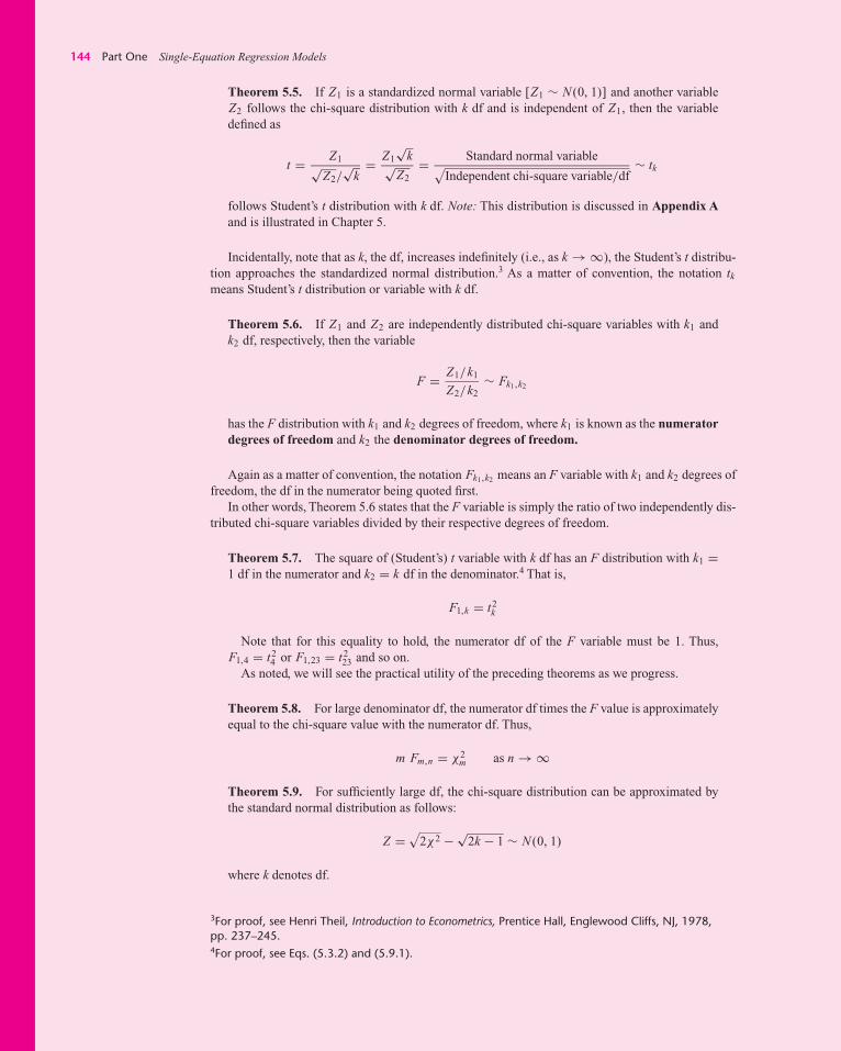
144 Part One Single-Equation Regression Models
Theorem 5.5. If Z1 is a standardized normal variable [Z1 ∼ N (0, 1)] and another variableZ2 follows the chi-square distribution with k df and is independent of Z1, then the variabledefined as
t = Z1√Z2/
√k
= Z1√
k√Z2
= Standard normal variable√Independent chi-square variable/df
∼ tk
follows Student’s t distribution with k df. Note: This distribution is discussed in Appendix Aand is illustrated in Chapter 5.
Incidentally, note that as k, the df, increases indefinitely (i.e., as k → ∞), the Student’s t distribu-tion approaches the standardized normal distribution.3 As a matter of convention, the notation tkmeans Student’s t distribution or variable with k df.
Theorem 5.6. If Z1 and Z2 are independently distributed chi-square variables with k1 andk2 df, respectively, then the variable
F = Z1/k1
Z2/k2∼ Fk1,k2
has the F distribution with k1 and k2 degrees of freedom, where k1 is known as the numeratordegrees of freedom and k2 the denominator degrees of freedom.
Again as a matter of convention, the notation Fk1,k2 means an F variable with k1 and k2 degrees offreedom, the df in the numerator being quoted first.
In other words, Theorem 5.6 states that the F variable is simply the ratio of two independently dis-tributed chi-square variables divided by their respective degrees of freedom.
Theorem 5.7. The square of (Student’s) t variable with k df has an F distribution with k1 =1 df in the numerator and k2 = k df in the denominator.4 That is,
F1,k = t2k
Note that for this equality to hold, the numerator df of the F variable must be 1. Thus,F1,4 = t2
4 or F1,23 = t223 and so on.
As noted, we will see the practical utility of the preceding theorems as we progress.
Theorem 5.8. For large denominator df, the numerator df times the F value is approximatelyequal to the chi-square value with the numerator df. Thus,
m Fm,n = χ2m as n → ∞
Theorem 5.9. For sufficiently large df, the chi-square distribution can be approximated bythe standard normal distribution as follows:
Z =√
2χ2 − √2k − 1 ∼ N (0, 1)
where k denotes df.
3For proof, see Henri Theil, Introduction to Econometrics, Prentice Hall, Englewood Cliffs, NJ, 1978,pp. 237–245.4For proof, see Eqs. (5.3.2) and (5.9.1).
guj75772_ch05.qxd 07/08/2008 12:46 PM Page 144
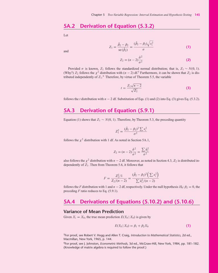
Chapter 5 Two-Variable Regression: Interval Estimation and Hypothesis Testing 145
5A.2 Derivation of Equation (5.3.2)
Let
Z1 = β2 − β2
se (β2)=
(β2 − β2)√
x2i
σ(1)
and
Z2 = (n − 2)σ 2
σ 2(2)
Provided σ is known, Z1 follows the standardized normal distribution; that is, Z1 ∼ N (0, 1).(Why?) Z2 follows the χ2 distribution with (n − 2) df.5 Furthermore, it can be shown that Z2 is dis-tributed independently of Z1.6 Therefore, by virtue of Theorem 5.5, the variable
t = Z1√
n − 2√Z2
(3)
follows the t distribution with n − 2 df. Substitution of Eqs. (1) and (2) into Eq. (3) gives Eq. (5.3.2).
5A.3 Derivation of Equation (5.9.1)
Equation (1) shows that Z1 ∼ N (0, 1). Therefore, by Theorem 5.3, the preceding quantity
Z21 = (β2 − β2)2 ∑
x2i
σ 2
follows the χ2 distribution with 1 df. As noted in Section 5A.1,
Z2 = (n − 2)σ 2
σ 2=
∑u2
i
σ 2
also follows the χ2 distribution with n − 2 df. Moreover, as noted in Section 4.3, Z2 is distributed in-dependently of Z1. Then from Theorem 5.6, it follows that
F = Z21/1
Z2/(n − 2)=
(β2 − β2)2(∑
x2i
)∑
u2i /(n − 2)
follows the F distribution with 1 and n − 2 df, respectively. Under the null hypothesis H0: β2 = 0, thepreceding F ratio reduces to Eq. (5.9.1).
5A.4 Derivations of Equations (5.10.2) and (5.10.6)
Variance of Mean PredictionGiven Xi = X0, the true mean prediction E(Y0 | X0) is given by
E(Y0 | X0) = β1 + β2 X0 (1)
5For proof, see Robert V. Hogg and Allen T. Craig, Introduction to Mathematical Statistics, 2d ed.,Macmillan, New York, 1965, p. 144.6For proof, see J. Johnston, Econometric Methods, 3d ed., McGraw-Hill, New York, 1984, pp. 181–182.(Knowledge of matrix algebra is required to follow the proof.)
guj75772_ch05.qxd 07/08/2008 12:46 PM Page 145

146 Part One Single-Equation Regression Models
We estimate Eq. (1) from
Y0 = β1 + β2 X0 (2)
Taking the expectation of Eq. (2), given X0, we get
E(Y0) = E(β1) + E(β2)X0
= β1 + β2 X0
because β1 and β2 are unbiased estimators. Therefore,
E(Y0) = E(Y0 | X0) = β1 + β2 X0 (3)
That is, Y0 is an unbiased predictor of E(Y0 | X0).Now using the property that var (a + b) = var (a) + var (b) + 2 cov (a, b) , we obtain
var (Y0) = var (β1) + var (β2)X20 + 2 cov (β1β2)X0 (4)
Using the formulas for variances and covariance of β1 and β2 given in Eqs. (3.3.1), (3.3.3), and(3.3.9) and manipulating terms, we obtain
var (Y0) = σ 2[
1
n+ (X0 − X)2∑
x2i
]= (5.10.2)
Variance of Individual PredictionWe want to predict an individual Y corresponding to X = X0; that is, we want to obtain
Y0 = β1 + β2 X0 + u0 (5)
We predict this as
Y0 = β1 + β2 X0 (6)
The prediction error, Y0 − Y0, is
Y0 − Y0 = β1 + β2 X0 + u0 − (β1 + β2 X0)
= (β1 − β1) + (β2 − β2)X0 + u0 (7)
Therefore,
E(Y0 − Y0) = E(β1 − β1) + E(β2 − β2)X0 − E(u0)
= 0
because β1, β2 are unbiased, X0 is a fixed number, and E(u0) is zero by assumption.Squaring Eq. (7) on both sides and taking expectations, we get var (Y0 − Y0) =
var (β1) + X20 var (β2) + 2X0 cov (β1, β2) + var (u0). Using the variance and covariance formulas
for β1 and β2 given earlier, and noting that var (u0) = σ 2, we obtain
var (Y0 − Y0) = σ 2[
1 + 1
n+ (X0 − X)2∑
x2i
]= (5.10.6)
guj75772_ch05.qxd 07/08/2008 12:46 PM Page 146

147
Some aspects of linear regression analysis can be easily introduced within the frameworkof the two-variable linear regression model that we have been discussing so far. First weconsider the case of regression through the origin, that is, a situation where the inter-cept term, β1, is absent from the model. Then we consider the question of the units ofmeasurement, that is, how the Y and X variables are measured and whether a change in theunits of measurement affects the regression results. Finally, we consider the question of thefunctional form of the linear regression model. So far we have considered models thatare linear in the parameters as well as in the variables. But recall that the regression theorydeveloped in the previous chapters requires only that the parameters be linear; the variablesmay or may not enter linearly in the model. By considering models that are linear in theparameters but not necessarily in the variables, we show in this chapter how the two-variable models can deal with some interesting practical problems.
Once the ideas introduced in this chapter are grasped, their extension to multipleregression models is quite straightforward, as we shall show in Chapters 7 and 8.
6.1 Regression through the Origin
There are occasions when the two-variable population regression function (PRF) assumesthe following form:
(6.1.1)
In this model the intercept term is absent or zero, hence the name regression through theorigin.
As an illustration, consider the capital asset pricing model (CAPM) of modern portfoliotheory, which, in its risk-premium form, may be expressed as1
(ER i − r f ) = βi (ERm − r f ) (6.1.2)
Yi = β2 Xi + ui
Chapter 6Extensions of theTwo-Variable LinearRegression Model
1See Haim Levy and Marshall Sarnat, Portfolio and Investment Selection: Theory and Practice, Prentice-Hall International, Englewood Cliffs, NJ, 1984, Chap. 14.
guj75772_ch06.qxd 07/08/2008 07:00 PM Page 147

148 Part One Single-Equation Regression Models
where ERi = expected rate of return on security iERm = expected rate of return on the market portfolio as represented by, say, the
S&P 500 composite stock index rf = risk-free rate of return, say, the return on 90-day Treasury billsβi = the Beta coefficient, a measure of systematic risk, i.e., risk that cannot be
eliminated through diversification. Also, a measure of the extent to whichthe ith security’s rate of return moves with the market. A βi > 1 implies avolatile or aggressive security, whereas a βi < 1 suggests a defensive secu-rity. (Note: Do not confuse this βi with the slope coefficient of the two-variable regression, β2.)
If capital markets work efficiently, then CAPM postulates that security i’s expected riskpremium (= ERi − rf) is equal to that security’s β coefficient times the expected marketrisk premium (= ERm − rf). If the CAPM holds, we have the situation depicted in Fig-ure 6.1. The line shown in the figure is known as the security market line (SML).
For empirical purposes, Equation 6.1.2 is often expressed as
R i − r f = βi (Rm − r f ) + ui (6.1.3)or
R i − r f = αi + βi (Rm − r f ) + ui (6.1.4)
The latter model is known as the Market Model.2 If CAPM holds, αi is expected to bezero. (See Figure 6.2.)
In passing, note that in Equation 6.1.4 the dependent variable, Y, is (Ri − rf) and theexplanatory variable, X, is βi, the volatility coefficient, and not (Rm − rf). Therefore, to runregression Eq. (6.1.4), one must first estimate βi, which is usually derived from thecharacteristic line, as described in Exercise 5.5. (For further details, see Exercise 8.28.)
As this example shows, sometimes the underlying theory dictates that the interceptterm be absent from the model. Other instances where the zero-intercept model may beappropriate are Milton Friedman’s permanent income hypothesis, which states that perma-nent consumption is proportional to permanent income; cost analysis theory, where it is
1
ER i – rf
Security market line
0 βi
ER i – rfFIGURE 6.1Systematic risk.
2See, for instance, Diana R. Harrington, Modern Portfolio Theory and the Capital Asset Pricing Model: AUser’s Guide, Prentice Hall, Englewood Cliffs, NJ, 1983, p. 71.
guj75772_ch06.qxd 07/08/2008 07:00 PM Page 148

Chapter 6 Extensions of the Two-Variable Linear Regression Model 149
postulated that the variable cost of production is proportional to output; and some versionsof monetarist theory that state that the rate of change of prices (i.e., the rate of inflation) isproportional to the rate of change of the money supply.
How do we estimate models like Eq. (6.1.1), and what special problems do they pose? Toanswer these questions, let us first write the sample regression function (SRF) of Eq. (6.1.1),namely,
Yi = β2 Xi + ui (6.1.5)
Now applying the ordinary least squares (OLS) method to Eq. (6.1.5), we obtain the fol-lowing formulas for β2 and its variance (proofs are given in Appendix 6A, Section 6A.1):
β2 =∑
Xi Yi∑X2
i
(6.1.6)
var (β2) = σ 2∑X2
i
(6.1.7)
where σ2 is estimated by
σ 2 =∑
u2i
n − 1(6.1.8)
It is interesting to compare these formulas with those obtained when the intercept term isincluded in the model:
β2 =∑
xi yi∑x2
i
(3.1.6)
var (β2) = σ 2∑x2
i
(3.3.1)
σ 2 =∑
u2i
n − 2(3.3.5)
βiSystematic risk
Sec
uri
ty r
isk
pre
miu
m
0
Ri – rfFIGURE 6.2The Market Modelof Portfolio Theory(assuming αi = 0).
guj75772_ch06.qxd 07/08/2008 07:00 PM Page 149

150 Part One Single-Equation Regression Models
The differences between the two sets of formulas should be obvious: In the model with theintercept term absent, we use raw sums of squares and cross products but in the intercept-present model, we use adjusted (from mean) sums of squares and cross products. Second,the df for computing σ 2 is (n − 1) in the first case and (n − 2) in the second case. (Why?)
Although the interceptless or zero intercept model may be appropriate on occasions,there are some features of this model that need to be noted. First,
∑ui , which is always
zero for the model with the intercept term (the conventional model), need not be zero whenthat term is absent. In short,
∑u i need not be zero for the regression through the origin.
Second, r2, the coefficient of determination introduced in Chapter 3, which is always non-negative for the conventional model, can on occasions turn out to be negative for the inter-ceptless model! This anomalous result arises because the r2 introduced in Chapter 3explicitly assumes that the intercept is included in the model. Therefore, the conventionallycomputed r2 may not be appropriate for regression-through-the-origin models.3
r 2 for Regression-through-Origin ModelAs just noted, and as further discussed in Appendix 6A, Section 6A.1, the conventional r2
given in Chapter 3 is not appropriate for regressions that do not contain the intercept. Butone can compute what is known as the raw r2 for such models, which is defined as
raw r2 =(∑
Xi Yi
)2
∑X2
i
∑Y 2
i
(6.1.9)
Note: These are raw (i.e., not mean-corrected) sums of squares and cross products.Although this raw r2 satisfies the relation 0 < r2 < 1, it is not directly comparable to the
conventional r2 value. For this reason some authors do not report the r2 value for zerointercept regression models.
Because of these special features of this model, one needs to exercise great caution inusing the zero intercept regression model. Unless there is very strong a priori expectation,one would be well advised to stick to the conventional, intercept-present model. This has adual advantage. First, if the intercept term is included in the model but it turns out to be sta-tistically insignificant (i.e., statistically equal to zero), for all practical purposes we have aregression through the origin.4 Second, and more important, if in fact there is an interceptin the model but we insist on fitting a regression through the origin, we would be commit-ting a specification error. We will discuss this more in Chapter 7.
3For additional discussion, see Dennis J. Aigner, Basic Econometrics, Prentice Hall, Englewood Cliffs, NJ,1971, pp. 85–88.4Henri Theil points out that if the intercept is in fact absent, the slope coefficient may be estimatedwith far greater precision than with the intercept term left in. See his Introduction to Econometrics,Prentice Hall, Englewood Cliffs, NJ, 1978, p. 76. See also the numerical example given next.5These data, originally obtained from DataStream databank, are reproduced from Christiaan Heij et al.,Econometrics Methods with Applications in Business and Economics, Oxford University Press, Oxford,U.K., 2004.
EXAMPLE 6.1 Table 6.1 gives data on excess returns Yt (%) on an index of 104 stocks in the sector ofcyclical consumer goods and excess returns Xt (%) on the overall stock market index forthe U.K. for the monthly data for the period 1980–1999, for a total of 240 observations.5
Excess return refers to return in excess of return on a riskless asset (see the CAPM model).
guj75772_ch06.qxd 07/08/2008 07:00 PM Page 150

OBS Y X OBS Y X
TABLE 6.1
1984:12 3.52786616 3.1915547631985:01 4.554587707 3.9078386881985:02 5.365478677 �1.7085674841985:03 4.525231564 0.4352184921985:04 2.944654344 0.9580678451985:05 �0.268599528 1.0954773751985:06 �3.661040481 �6.8161089091985:07 �4.540505062 2.7850543541985:08 9.195292816 3.9002090231985:09 �1.894817019 �4.2030044141985:10 12.00661274 5.601798021985:11 1.233987382 1.5700939761985:12 �1.446329607 �1.0844271211986:01 6.023618851 0.7786694731986:02 10.51235756 6.4706512621986:03 13.40071024 8.9537811921986:04 �7.796262998 �2.3877616851986:05 0.211540446 �2.8738385881986:06 6.471111064 3.4402690981986:07 �9.037475168 �5.8910533751986:08 �5.47838091 6.3755820041986:09 �6.756881852 �5.7348393961986:10 �2.564960223 3.630884081986:11 2.456599468 �1.316066871986:12 1.476421303 3.5216012161987:01 17.0694004 8.6734128961987:02 7.565726727 6.9143619231987:03 �3.239325817 �0.4606608541987:04 3.662578335 4.2959760771987:05 7.157455113 7.7196925291987:06 4.774901623 3.0398876221987:07 4.23770166 2.5102238041987:08 �0.881352219 �3.0394435631987:09 11.49688416 3.7870920181987:10 �35.56617624 �27.869693111987:11 �14.59137369 �9.9563670941987:12 14.87271664 7.9758659481988:01 1.748599294 3.9369383981988:02 �0.606016446 �0.327970641988:03 �6.078095523 �2.1615442021988:04 3.976153828 2.7217878421988:05 �1.050910058 �0.5148254221988:06 3.317856956 3.1287964821988:07 0.407100105 0.1815020751988:08 �11.87932524 �7.8923637861988:09 �8.801026046 3.3470818991988:10 6.784211277 3.1585921441988:11 �10.20578119 �4.8164703631988:12 �6.73805381 �0.0085499971989:01 12.83903643 13.460982191989:02 3.302860922 �0.7644746921989:03 �0.155918301 2.2984910971989:04 3.623090767 0.7620745881989:05 �1.167680873 �0.4957961171989:06 �1.221603303 1.2066360131989:07 5.262902744 4.6370261161989:08 4.845013219 2.6808741161989:09 �5.069564838 �5.3038580351989:10 �13.57963526 �7.210655599
1980:01 6.08022852 7.2634484041980:02 �0.924185461 6.3398955041980:03 �3.286174252 �9.2852168341980:04 5.211976571 0.7932907711980:05 �16.16421111 �2.9024209851980:06 �1.054703649 8.6131508751980:07 11.17237699 3.9820628481980:08 �11.06327551 �1.1501709071980:09 �16.77699609 3.4861258681980:10 �7.021834032 4.3298502781980:11 �9.71684668 0.9368752791980:12 5.215705717 �5.2024558461981:01 �6.612000956 �2.0827575091981:02 4.264498443 2.7285228931981:03 4.916710821 0.6533971061981:04 22.20495946 6.4360719621981:05 �11.29868524 �4.2591979321981:06 �5.770507783 0.5439097071981:07 �5.217764717 �0.4868459331981:08 16.19620175 2.8439995081981:09 �17.16995395 �16.45721421981:10 1.105334728 4.4689381711981:11 11.6853367 5.8855196581981:12 �2.301451728 �0.3906981641982:01 8.643728679 2.4995678961982:02 �11.12907503 �4.0336070751982:03 1.724627956 3.0425257771982:04 0.157879967 0.7345646651982:05 �1.875202616 2.7797322881982:06 �10.62481767 �5.9001165761982:07 �5.761135416 3.0053443851982:08 5.481432596 3.9549906191982:09 �17.02207459 2.5471270671982:10 7.625420708 4.3290081061982:11 �6.575721646 0.1919405941982:12 �2.372829861 �0.921675551983:01 17.52374936 3.3946825771983:02 1.354655809 0.7587143531983:03 16.26861049 1.8620736641983:04 �6.074547158 6.7977513411983:05 �0.826650702 �1.6992536281983:06 3.807881996 4.0925924021983:07 0.57570091 �2.9262992621983:08 3.755563441 1.7734243061983:09 �5.365927271 �2.8008156671983:10 �3.750302815 �1.5053949951983:11 4.898751703 4.186962841983:12 4.379256151 1.2014169811984:01 16.56016188 6.7693207881984:02 1.523127464 �1.6860274171984:03 1.0206078 5.2458061051984:04 �3.899307684 1.7287102641984:05 �14.32501615 �7.2790755951984:06 3.056627177 �0.779470671984:07 �0.02153592 �2.4396344871984:08 3.355102212 8.4459778131984:09 0.100006778 1.2210801291984:10 1.691250318 2.7333867721984:11 8.20075301 5.12753329
(Continued )
151
guj75772_ch06.qxd 07/08/2008 07:00 PM Page 151

1989:11 1.100607603 5.3501859441989:12 4.925083189 4.1062458551990:01 �2.532068851 �3.6295473741990:02 �6.601872876 �5.2058042991990:03 �1.023768943 �2.1832448631990:04 �7.097917266 �5.4085637941990:05 6.376626925 10.575991691990:06 1.861974711 �0.3386120991990:07 �5.591527585 �2.213162021990:08 �15.31758975 �8.4761774271990:09 �10.17227358 �7.459414711990:10 �2.217396045 �0.0858877631990:11 5.974205798 5.0347705341990:12 �0.857289036 �1.7677149081991:01 �3.780184589 0.1891084561991:02 20.64721437 10.387415041991:03 10.94068018 2.9219138271991:04 �3.145639589 0.9717201881991:05 �3.142887645 �0.43178191991:06 �1.960866141 �3.3429249861991:07 7.330964031 5.2428115091991:08 7.854387926 2.8806546911991:09 2.539177843 �1.1214722241991:10 �1.233244642 �3.9695779561991:11 �11.7460404 �5.7079950621991:12 1.078226286 1.5025670491992:01 5.937904622 2.5995650941992:02 4.113184542 0.1358810871992:03 �0.655199392 �6.1461380641992:04 15.28430278 10.457368311992:05 3.994517585 1.4159870461992:06 �11.94450998 �8.2611094241992:07 �2.530701327 �3.7788121671992:08 �9.842366221 �5.3868184881992:09 18.11573724 11.194363721992:10 0.200950206 3.9998700381992:11 1.125853097 3.6206747521992:12 7.639180786 2.8872222511993:01 2.919569408 1.3367460911993:02 �1.062404105 1.2402738461993:03 1.292641409 0.4071443121993:04 0.420241384 �1.7349300471993:05 �2.514080553 1.1115336871993:06 0.419362276 1.3541277421993:07 4.374024535 1.9430615681993:08 1.733528075 4.9619798271993:09 �3.659808969 �1.6187299361993:10 5.85690764 4.2154086081993:11 �1.365550294 1.8803601651993:12 �1.346979017 5.8263524131994:01 12.89578758 2.9735406931994:02 �5.346700561 �5.4798585631994:03 �7.614726564 �5.7845470881994:04 10.22042923 1.1570834381994:05 �6.928422261 �6.3561994931994:06 �5.065919037 �0.8435838881994:07 7.483498556 5.7799532241994:08 1.828762662 3.2981301841994:09 �5.69293279 �7.1100100851994:10 �2.426962489 2.9680055971994:11 2.125100668 �1.531245158
1994:12 �4.225370964 0.2642802591995:01 �6.302392617 �2.4203884311995:02 1.27867637 0.1387952131995:03 10.90890516 3.2316565851995:04 2.497849434 2.2158046821995:05 2.891526594 3.8568135891995:06 �3.773000069 �0.9522043061995:07 8.776288715 4.0200363631995:08 2.88256097 1.4236003451995:09 2.14691333 �0.0379125711995:10 �4.590104662 �1.176553291995:11 �1.293255187 3.7602773561995:12 �4.244101531 0.4346263571996:01 6.647088904 1.9063451031996:02 1.635900742 0.3018989611996:03 7.8581899 �0.3141323241996:04 0.789544896 3.0343317411996:05 �0.907725397 �1.4973462991996:06 �0.392246948 �0.8946768541996:07 �1.035896351 �0.5328162741996:08 2.556816005 3.8637370881996:09 3.131830038 2.1182548971996:10 �0.020947358 �0.8535532621996:11 �5.312287782 1.7703409391996:12 �5.196176326 1.7025516351997:01 �0.753247124 3.4657533481997:02 �2.474343938 1.1152532211997:03 2.47647802 �2.0578184611997:04 �1.119104196 3.570899551997:05 3.352076269 1.9534804381997:06 �1.910172239 2.4587004041997:07 0.142814607 2.9923412971997:08 10.50199263 �0.4579680381997:09 12.98501943 8.1112789671997:10 �4.134761655 �6.9671245041997:11 �4.148579856 �0.1559247911997:12 �1.752478236 3.8532834331998:01 �3.349121498 7.3794660141998:02 14.07471304 4.2990978861998:03 7.791650968 3.4107805171998:04 5.154679109 �0.0814949931998:05 3.293686179 �1.6131311591998:06 �13.25461802 �0.3972889541998:07 �7.714205916 �2.2373652831998:08 �15.26340483 �12.46319931998:09 �15.22865141 �5.1707349851998:10 15.96218038 11.705447881998:11 �8.684089113 �0.3802002231998:12 17.13842369 4.9867051871999:01 �1.468448611 2.4937279941999:02 8.5036 0.9371052591999:03 10.8943073 4.2800825061999:04 13.03497394 3.9608244021999:05 �5.654671597 �4.4991980791999:06 8.321969316 3.6567456991999:07 0.507652273 �2.5039714731999:08 �5.022980561 �0.1219019231999:09 �2.305448839 �5.3880324321999:10 �1.876879466 4.0109897161999:11 1.348824769 6.2653129751999:12 �2.64164938 4.045658427
OBS Y X OBS Y X
152
guj75772_ch06.qxd 07/08/2008 07:00 PM Page 152

Chapter 6 Extensions of the Two-Variable Linear Regression Model 153
First we fit model (6.1.3) to these data. Using EViews6 we obtained the followingregression results, which are given in the standard EViews format.
Dependent Variable: YMethod: Least SquaresSample: 1980M01 1999M12Included observations: 240
Coefficient Std. Error t-Statistic Prob.
X 1.155512 0.074396 15.53200 0.0000
R-squared 0.500309 Mean dependent var. 0.499826Adjusted R-squared† 0.500309 S.D. dependent var. 7.849594S.E. of regression 5.548786 Durbin-Watson stat.* 1.972853Sum squared resid. 7358.578
*We will discuss this statistic in Chapter 12.†See Chapter 7.
As these results show, the slope coefficient, which is the Beta coefficient, is highly significant,for its p value is extremely small. The interpretation here is that if the excess market rate goesup by 1 percentage point, the excess return on the index of consumer goods sector goes upby about 1.15 percentage points. Not only is the slope coefficient statistically significant, butit is significantly greater than 1 (can you verify this?). If a Beta coefficient is greater than 1,such a security (here a portifolio of 104 stocks) is said to be volatile; it moves more thanproportionately with the overall stock market index. But this finding should not be surprising,for in this example we are considering stocks from the sector of cyclical consumer goods suchas houshold durables, automobiles, textiles, and sports equipment.
If we fit model (6.1.4), we obtain the following results:
Dependent Variable: YMethod: Least SquaresSample: 1980M01 1999M12Included observations: 240
Coefficient Std. Error t-Statistic Prob.
C −0.447481 0.362943 �1.232924 0.2188X 1.171128 0.075386 15.53500 0.0000
R-squared 0.503480 Mean dependent var. 0.499826Adjusted R-squared 0.501394 S.D. dependent var. 7.849594S.E. of regression 5.542759 Durbin-Watson stat. 1.984746Sum squared resid. 7311.877 Prob. (F-statistic) 0.000000F-statistic 241.3363
From these results we see that the intercept is not statistically different from zero, althoughthe slope coefficient (the Beta coefficient) is highly statistically significant. This suggeststhat the regression-through-the-origin model fits the data well. Besides, statistically there isno difference in the value of the slope coefficient in the two models. Note that the standarderror of the slope coefficient in the regression-through-the-origin model is slightly lowerthan the one in the intercept-present model, thus supporting Theil’s argument given infootnote 4. Even then, the slope coefficient is statistically greater than 1, once again con-firming that returns on the stocks in the cyclical consumer goods sector are volatile.
By the way, note that the r2 value given for the regression-through-the-origin modelshould be taken with a grain of salt, for the traditional formula of r2 is not applicable for suchmodels. EViews, however, routinely presents the standard r2 value even for such models.
EXAMPLE 6.1(Continued)
guj75772_ch06.qxd 11/08/2008 03:50 PM Page 153

154 Part One Single-Equation Regression Models
6.2 Scaling and Units of Measurement
To grasp the ideas developed in this section, consider the data given in Table 6.2, whichrefers to U.S. gross private domestic investment (GPDI) and gross domestic product (GDP),in billions as well as millions of (chained) 2000 dollars.
Suppose in the regression of GPDI on GDP one researcher uses data in billions of dol-lars but another expresses data in millions of dollars. Will the regression results be the samein both cases? If not, which results should one use? In short, do the units in which theregressand and regressor(s) are measured make any difference in the regression results? Ifso, what is the sensible course to follow in choosing units of measurement for regressionanalysis? To answer these questions, let us proceed systematically. Let
Yi = β1 + β2 Xi + u i (6.2.1)
where Y = GPDI and X = GDP. Define
Y ∗i = w1Yi (6.2.2)
X∗i = w2 Xi (6.2.3)
where w1 and w2 are constants, called the scale factors; w1 may equal w2 or be different.From Equations 6.2.2 and 6.2.3 it is clear that Y ∗
i and X∗i are rescaled Yi and Xi . Thus,
if Yi and Xi are measured in billions of dollars and one wants to express them in millionsof dollars, we will have Y ∗
i = 1000 Yi and X∗i = 1000 Xi ; here w1 = w2 = 1000.
Now consider the regression using Y ∗i and X∗
i variables:
Y ∗i = β∗
1 + β∗2 X∗
i + u∗i (6.2.4)
where Y ∗i = w1Yi , X∗
i = w2 Xi , and u∗i = w1ui . (Why?)
TABLE 6.2Gross PrivateDomestic Investmentand GDP, UnitedStates, 1990–2005(Billions of chained[2000] dollars, exceptas noted; quarterlydata at seasonallyadjusted annualrates)
Year GPDIBL GPDIM GDPB GDPM
1990 886.6 886,600.0 7,112.5 7,112,500.01991 829.1 829,100.0 7,100.5 7,100,500.01992 878.3 878,300.0 7,336.6 7,336,600.01993 953.5 953,500.0 7,532.7 7,532,700.01994 1,042.3 1,042,300.0 7,835.5 7,835,500.01995 1,109.6 1,109,600.0 8,031.7 8,031,700.01996 1,209.2 1,209,200.0 8,328.9 8,328,900.01997 1,320.6 1,320,600.0 8,703.5 8,703,500.01998 1,455.0 1,455,000.0 9,066.9 9,066,900.01999 1,576.3 1,576,300.0 9,470.3 9,470,300.02000 1,679.0 1,679,000.0 9,817.0 9,817,000.02001 1,629.4 1,629,400.0 9,890.7 9,890,700.02002 1,544.6 1,544,600.0 10,048.8 10,048,800.02003 1,596.9 1,596,900.0 10,301.0 10,301,000.02004 1,713.9 1,713,900.0 10,703.5 10,703,500.02005 1,842.0 1,842,000.0 11,048.6 11,048,600.0
Note: GPDIBL = gross private domestic investment, billions of 2000 dollars.GPDIM = gross private domestic investments, millions of 2000 dollars.
GDPB = gross domestic product, billions of 2000 dollars.GDPM = gross domestic product, millions of 2000 dollars.
Source: Economic Report of the President, 2007, Table B-2, p. 328.
guj75772_ch06.qxd 07/08/2008 07:00 PM Page 154

Chapter 6 Extensions of the Two-Variable Linear Regression Model 155
We want to find out the relationships between the following pairs:
1. β1 and β∗1
2. β2 and β∗2
3. var (β1) and var (β∗1 )
4. var (β2) and var (β∗2 )
5. σ 2 and σ ∗2
6. r2xy and r2
x∗ y∗
From least-squares theory we know (see Chapter 3) that
β1 = Y − β2 X (6.2.5)
β2 =∑
xi yi∑x2
i
(6.2.6)
var (β1) =∑
X2i
n∑
x2i
· σ 2 (6.2.7)
var (β2) = σ 2∑x2
i
(6.2.8)
σ 2 =∑
u2i
n − 2(6.2.9)
Applying the OLS method to Equation 6.2.4, we obtain similarly
β∗1 = Y ∗ − β∗
2 X∗ (6.2.10)
β∗2 =
∑x∗
i y∗i∑
x∗2i
(6.2.11)
var (β∗1 ) =
∑X∗2
i
n∑
x∗2i
· σ ∗2 (6.2.12)
var (β∗2 ) = σ ∗2∑
x∗2i
(6.2.13)
σ ∗2 =∑
u∗2i
(n − 2)(6.2.14)
From these results it is easy to establish relationships between the two sets of parameterestimates. All that one has to do is recall these definitional relationships: Y ∗
i = w1Yi (ory∗
i = w1 yi ); X∗i = w2 Xi (or x∗
i = w2xi ); u∗i = w1ui ; Y ∗ = w1Y ; and X∗ = w2 X . Making
use of these definitions, the reader can easily verify that
β∗2 =
(w1
w2
)β2 (6.2.15)
β∗1 = w1β1 (6.2.16)
σ ∗2 = w21σ
2 (6.2.17)
var (β∗1 ) = w2
1 var (β1) (6.2.18)
guj75772_ch06.qxd 07/08/2008 07:00 PM Page 155

156 Part One Single-Equation Regression Models
var (β∗2 ) =
(w1
w2
)2
var (β2) (6.2.19)
r2xy = r2
x∗ y∗ (6.2.20)
From the preceding results it should be clear that, given the regression results based onone scale of measurement, one can derive the results based on another scale of measure-ment once the scaling factors, the w’s, are known. In practice, though, one should choosethe units of measurement sensibly; there is little point in carrying all those zeros inexpressing numbers in millions or billions of dollars.
From the results given in (6.2.15) through (6.2.20) one can easily derive some specialcases. For instance, if w1 = w2, that is, the scaling factors are identical, the slope coefficientand its standard error remain unaffected in going from the (Yi , Xi ) to the (Y ∗
i , X∗i ) scale,
which should be intuitively clear. However, the intercept and its standard error are both mul-tiplied by w1. But if the X scale is not changed (i.e., w2 = 1) and the Y scale is changed bythe factor w1, the slope as well as the intercept coefficients and their respective standarderrors are all multiplied by the same w1 factor. Finally, if the Y scale remains unchanged (i.e.,w1 = 1) but the X scale is changed by the factor w2, the slope coefficient and its standarderror are multiplied by the factor (1/w2) but the intercept coefficient and its standard errorremain unaffected.
It should, however, be noted that the transformation from the (Y, X ) to the (Y ∗, X∗) scaledoes not affect the properties of the OLS estimators discussed in the preceding chapters.
EXAMPLE 6.2The Relationshipbetween theGDPI and GDP,United States,1990–2005
To substantiate the preceding theoretical results, let us return to the data given inTable 6.2 and examine the following results (numbers in parentheses are the estimatedstandard errors).
Both GPDI and GDP in billions of dollars:
GPDIt = −926.090 + 0.2535 GDPt
se = (116.358) (0.0129) r2 = 0.9648 (6.2.21)
Both GPDI and GDP in millions of dollars:
GPDIt = −926,090 + 0.2535 GDPt
se = (116,358) (0.0129) r2 = 0.9648 (6.2.22)
Notice that the intercept as well as its standard error is 1000 times the corresponding val-ues in the regression (6.2.21) (note that w1 = 1000 in going from billions to millions ofdollars), but the slope coefficient as well as its standard error is unchanged, in accordancewith the theory.
GPDI in billions of dollars and GDP in millions of dollars:
GPDIt = −926.090 + 0.0002535 GDPt
se = (116.358) (0.0000129) r2 = 0.9648 (6.2.23)
As expected, the slope coefficient as well as its standard error is 1/1000 its value inEq. (6.2.21), since only the X, or GDP, scale is changed.
GPDI in millions of dollars and GDP in billions of dollars:
GPDIt = −926,090 + 253.524 GDPt
se = (116,358.7) (12.9465) r2 = 0.9648 (6.2.24)
guj75772_ch06.qxd 07/08/2008 07:00 PM Page 156

Chapter 6 Extensions of the Two-Variable Linear Regression Model 157
A Word about InterpretationSince the slope coefficient β2 is simply the rate of change, it is measured in the units of theratio
Units of the dependent variable
Units of the explanatory variable
Thus in regression (6.2.21) the interpretation of the slope coefficient 0.2535 is thatif GDP changes by a unit, which is 1 billion dollars, GPDI on the average changes by0.2535 billion dollars. In regression (6.2.23) a unit change in GDP, which is 1 milliondollars, leads on average to a 0.0002535 billion dollar change in GPDI. The two results areof course identical in the effects of GDP on GPDI; they are simply expressed in differentunits of measurement.
6.3 Regression on Standardized Variables
We saw in the previous section that the units in which the regressand and regressor(s) areexpressed affect the interpretation of the regression coefficients. This can be avoided ifwe are willing to express the regressand and regressor(s) as standardized variables. A vari-able is said to be standardized if we subtract the mean value of the variable from itsindividual values and divide the difference by the standard deviation of that variable.
Thus, in the regression of Y and X, if we redefine these variables as
Y ∗i = Yi − Y
SY(6.3.1)
X∗i = Xi − X
SX(6.3.2)
where Y = sample mean of Y, SY = sample standard deviation of Y, X = sample meanof X, and SX is the sample standard deviation of X; the variables Y ∗
i and X∗i are called
standardized variables.An interesting property of a standardized variable is that its mean value is always zero
and its standard deviation is always 1. (For proof, see Appendix 6A, Section 6A.2.)As a result, it does not matter in what unit the regressand and regressor(s) are measured.
Therefore, instead of running the standard (bivariate) regression:
Yi = β1 + β2 Xi + ui (6.3.3)
we could run regression on the standardized variables as
Y ∗i = β∗
1 + β∗2 X∗
i + u∗i (6.3.4)
= β∗2 X∗
i + u∗i (6.3.5)
Again notice that both the intercept and the slope coefficients as well as their respectivestandard errors are 1000 times their values in Eq. (6.2.21), in accordance with our theo-retical results.
Notice that in all the regressions presented above, the r2 value remains the same, whichis not surprising because the r2 value is invariant to changes in the unit of measurement,as it is a pure, or dimensionless, number.
EXAMPLE 6.2(Continued)
guj75772_ch06.qxd 07/08/2008 07:00 PM Page 157

158 Part One Single-Equation Regression Models
since it is easy to show that, in the regression involving standardized regressand andregressor(s), the intercept term is always zero.6 The regression coefficients of the standard-ized variables, denoted by β∗
1 and β∗2 , are known in the literature as the beta coefficients.7
Incidentally, notice that (6.3.5) is a regression through the origin.How do we interpret the beta coefficients? The interpretation is that if the (standardized)
regressor increases by one standard deviation, on average, the (standardized) regressandincreases by β∗
2 standard deviation units. Thus, unlike the traditional model in Eq. (6.3.3), wemeasure the effect not in terms of the original units in which Y and X are expressed, but instandard deviation units.
To show the difference between Eqs. (6.3.3) and (6.3.5), let us return to the GPDI andGDP example discussed in the preceding section. The results of (6.2.21) discussed previ-ously are reproduced here for convenience.
GPDIt = −926.090 + 0.2535 GDPt (6.3.6)se = (116.358) (0.0129) r2 = 0.9648
where GPDI and GDP are measured in billions of dollars.The results corresponding to Eq. (6.3.5) are as follows, where the starred variables are
standardized variables:
GPDI∗t = 0.9822 GDP∗
t (6.3.7)se = (0.0485)
We know how to interpret Eq. (6.3.6): If GDP goes up by a dollar, on average GPDI goesup by about 25 cents. How about Eq. (6.3.7)? Here the interpretation is that if the (stan-dardized) GDP increases by one standard deviation, on average, the (standardized) GPDIincreases by about 0.98 standard deviations.
What is the advantage of the standardized regression model over the traditional model?The advantage becomes more apparent if there is more than one regressor, a topic wewill take up in Chapter 7. By standardizing all regressors, we put them on an equal basisand therefore can compare them directly. If the coefficient of a standardized regressor islarger than that of another standardized regressor appearing in that model, then the lattercontributes more relatively to the explanation of the regressand than the former. In otherwords, we can use the beta coefficients as a measure of relative strength of the variousregressors. But more on this in the next two chapters.
Before we leave this topic, two points may be noted. First, for the standardized regres-sion in Eq. (6.3.7) we have not given the r2 value because this is a regression throughthe origin for which the usual r2 is not applicable, as pointed out in Section 6.1. Second,there is an interesting relationship between the β coefficients of the conventional modeland the beta coefficients. For the bivariate case, the relationship is as follows:
β∗2 = β2
(S x
S y
)(6.3.8)
where Sx = the sample standard deviation of the X regressor and Sy = the sample standarddeviation of the regressand. Therefore, we can crisscross between the β and beta coefficients
6Recall from Eq. (3.1.7) that Intercept = Mean value of the dependent variable − Slope × Meanvalue of the regressor. But for the standardized variables the mean values of the dependent variableand the regressor are zero. Hence the intercept value is zero.7Do not confuse these beta coefficients with the beta coefficients of finance theory.
guj75772_ch06.qxd 07/08/2008 07:00 PM Page 158
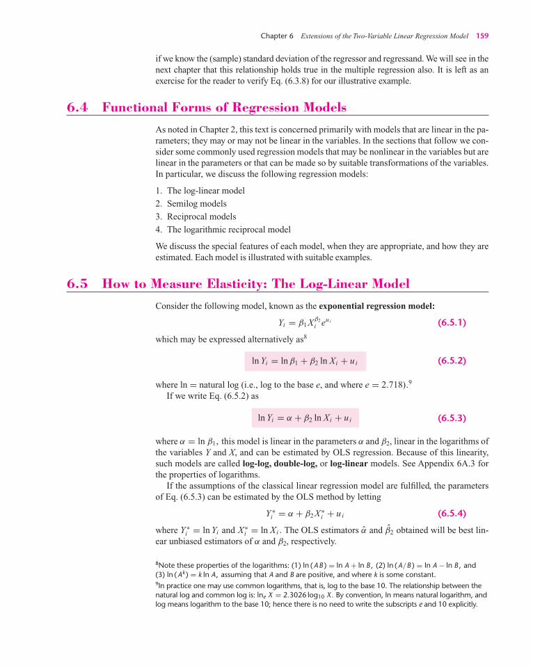
Chapter 6 Extensions of the Two-Variable Linear Regression Model 159
if we know the (sample) standard deviation of the regressor and regressand. We will see in thenext chapter that this relationship holds true in the multiple regression also. It is left as anexercise for the reader to verify Eq. (6.3.8) for our illustrative example.
6.4 Functional Forms of Regression Models
As noted in Chapter 2, this text is concerned primarily with models that are linear in the pa-rameters; they may or may not be linear in the variables. In the sections that follow we con-sider some commonly used regression models that may be nonlinear in the variables but arelinear in the parameters or that can be made so by suitable transformations of the variables.In particular, we discuss the following regression models:
1. The log-linear model
2. Semilog models
3. Reciprocal models
4. The logarithmic reciprocal model
We discuss the special features of each model, when they are appropriate, and how they areestimated. Each model is illustrated with suitable examples.
6.5 How to Measure Elasticity: The Log-Linear Model
Consider the following model, known as the exponential regression model:
Yi = β1 Xβ2
i eu i (6.5.1)
which may be expressed alternatively as8
(6.5.2)
where ln = natural log (i.e., log to the base e, and where e = 2.718).9
If we write Eq. (6.5.2) as
(6.5.3)
where α = ln β1, this model is linear in the parameters α and β2, linear in the logarithms ofthe variables Y and X, and can be estimated by OLS regression. Because of this linearity,such models are called log-log, double-log, or log-linear models. See Appendix 6A.3 forthe properties of logarithms.
If the assumptions of the classical linear regression model are fulfilled, the parametersof Eq. (6.5.3) can be estimated by the OLS method by letting
Y ∗i = α + β2 X∗
i + ui (6.5.4)
where Y ∗i = ln Yi and X∗
i = ln Xi . The OLS estimators α and β2 obtained will be best lin-ear unbiased estimators of α and β2, respectively.
ln Yi = α + β2 ln Xi + ui
ln Yi = ln β1 + β2 ln Xi + ui
8Note these properties of the logarithms: (1) ln (AB ) = ln A + ln B , (2) ln (A/B ) = ln A − ln B , and(3) ln (Ak) = k ln A, assuming that A and B are positive, and where k is some constant.9In practice one may use common logarithms, that is, log to the base 10. The relationship between thenatural log and common log is: lne X = 2.3026 log10 X. By convention, ln means natural logarithm, andlog means logarithm to the base 10; hence there is no need to write the subscripts e and 10 explicitly.
guj75772_ch06.qxd 07/08/2008 07:00 PM Page 159

160 Part One Single-Equation Regression Models
One attractive feature of the log-log model, which has made it popular in applied work,is that the slope coefficient β2 measures the elasticity of Y with respect to X, that is, the per-centage change in Y for a given (small) percentage change in X.10 Thus, if Y represents thequantity of a commodity demanded and X its unit price, β2 measures the price elasticity ofdemand, a parameter of considerable economic interest. If the relationship between quan-tity demanded and price is as shown in Figure 6.3a, the double-log transformation as shownin Figure 6.3b will then give the estimate of the price elasticity (−β2).
Two special features of the log-linear model may be noted: The model assumes thatthe elasticity coefficient between Y and X, β2, remains constant throughout (why?), hencethe alternative name constant elasticity model.11 In other words, as Figure 6.3b shows, thechange in ln Y per unit change in ln X (i.e., the elasticity, β2) remains the same no matter atwhich ln X we measure the elasticity. Another feature of the model is that although α andβ2 are unbiased estimates of α and β2, β1 (the parameter entering the original model) whenestimated as β1 = antilog (α) is itself a biased estimator. In most practical problems, how-ever, the intercept term is of secondary importance, and one need not worry about obtain-ing its unbiased estimate.12
(a)
PriceQ
uan
tity
dem
and
ed
Y
(b)
Log of price
Log
of
quan
tity
dem
and
ed
ln Y
ln X X
Y= β1Xi–β 2ββ lnY= ln β1– β2 ln Xiββ
FIGURE 6.3Constant elasticitymodel.
10The elasticity coefficient, in calculus notation, is defined as (dY/Y )/(dX/X) = [(dY/dX)(X/Y )].Readers familiar with differential calculus will readily see that β2 is in fact the elasticity coefficient.
A technical note: The calculus-minded reader will note that d(ln X)/dX = 1/X or d(ln X) = dX/X,that is, for infinitesimally small changes (note the differential operator d) the change in ln X is equalto the relative or proportional change in X. In practice, though, if the change in X is small, this rela-tionship can be written as: change in ln X =. relative change in X, where =. means approximately.Thus, for small changes,
(ln Xt − ln Xt−1) =. (Xt − Xt−1)/Xt−1 = relative change in X
Incidentally, the reader should note these terms, which will occur frequently: (1) absolute change,(2) relative or proportional change, and (3) percentage change, or percent growth rate.Thus, (Xt − Xt−1) represents absolute change, (Xt − Xt−1)/Xt−1 = (Xt/Xt−1 − 1) is relative orproportional change, and [(Xt − Xt−1)/Xt−1]100 is the percentage change, or the growth rate.Xt and Xt−1 are, respectively, the current and previous values of the variable X. 11A constant elasticity model will give a constant total revenue change for a given percentage changein price regardless of the absolute level of price. Readers should contrast this result with the elasticityconditions implied by a simple linear demand function, Yi = β1 + β2 Xi + ui . However, a simple linearfunction gives a constant quantity change per unit change in price. Contrast this with what the log-linear model implies for a given dollar change in price.12Concerning the nature of the bias and what can be done about it, see Arthur S. Goldberger, Topicsin Regression Analysis, Macmillan, New York, 1978, p. 120.
guj75772_ch06.qxd 07/08/2008 07:00 PM Page 160

Chapter 6 Extensions of the Two-Variable Linear Regression Model 161
In the two-variable model, the simplest way to decide whether the log-linear model fitsthe data is to plot the scattergram of ln Yi against ln Xi and see if the scatter points lieapproximately on a straight line, as in Figure 6.3b.
A cautionary note: The reader should be aware of the distinction between a percentchange and a percentage point change. For example, the unemployment rate is oftenexpressed in percent form, say, the unemployment rate of 6%. If this rate goes to 8%, we saythat the percentage point change in the unemployment rate is 2, whereas the percent changein the unemployment rate is (8 − 6)/6, or about 33%. So be careful when you deal withpercent and percentage point changes, for the two are very different concepts.
13Durable goods include motor vehicles and parts, furniture, and household equipment; nondurablegoods include food, clothing, gasoline and oil, fuel oil and coal; and services include housing, elec-tricity and gas, transportation, and medical care.
EXAMPLE 6.3Expenditureon DurableGoods inRelation toTotal PersonalConsumptionExpenditure
Table6.3presentsdataon totalpersonal consumptionexpenditure (PCEXP), expenditureondurable goods (EXPDUR), expenditure on nondurable goods (EXPNONDUR), and expendi-ture on services (EXPSERVICES), all measured in 2000 billions of dollars.13
Suppose we wish to find the elasticity of expenditure on durable goods with respectto total personal consumption expenditure. Plotting the log of expenditure on durablegoods against the log of total personal consumption expenditure, you will see that the relationship between the two variables is linear. Hence, the double-log model may beappropriate. The regression results are as follows:
ln EXDURt = −7.5417 + 1.6266 ln PCEXt
se = (0.7161) (0.0800) (6.5.5)t = (−10.5309)* (20.3152)* r2 = 0.9695
where * indicates that the p value is extremely small.
Year or quarter EXPSERVICES EXPDUR EXPNONDUR PCEXP
2003-I 4,143.3 971.4 2,072.5 7,184.92003-II 4,161.3 1,009.8 2,084.2 7,249.32003-III 4,190.7 1,049.6 2,123.0 7,352.92003-IV 4,220.2 1,051.4 2,132.5 7,394.32004-I 4,268.2 1,067.0 2,155.3 7,479.82004-II 4,308.4 1,071.4 2,164.3 7,534.42004-III 4,341.5 1,093.9 2,184.0 7,607.12004-IV 4,377.4 1,110.3 2,213.1 7,687.12005-I 4,395.3 1,116.8 2,241.5 7,739.42005-II 4,420.0 1,150.8 2,268.4 7,819.82005-III 4,454.5 1,175.9 2,287.6 7,895.32005-IV 4,476.7 1,137.9 2,309.6 7,910.22006-I 4,494.5 1,190.5 2,342.8 8,003.82006-II 4,535.4 1,190.3 2,351.1 8,055.02006-III 4,566.6 1,208.8 2,360.1 8,111.2
Note: See Table B-2 for data for total personal consumption expenditures for 1959–1989.EXPSERVICES = expenditure on services, billions of 2000 dollars.
EXPDUR = expenditure on durable goods, billions of 2000 dollars.EXPNONDUR = expenditure on nondurable goods, billions of 2000 dollars.
PCEXP = total personal consumption expenditure, billions of 2000 dollars.
TABLE 6.3 Total PersonalExpenditure andCategories(Billions of chained[2000] dollars;quarterly data atseasonally adjustedannual rates)
Sources: Department ofCommerce, Bureau ofEconomic Analysis.Economic Report of the President, 2007, Table B-17, p. 347.
(Continued )
guj75772_ch06.qxd 07/08/2008 07:07 PM Page 161

162 Part One Single-Equation Regression Models
6.6 Semilog Models: Log–Lin and Lin–Log Models
How to Measure the Growth Rate: The Log–Lin ModelEconomists, businesspeople, and governments are often interested in finding out the rate ofgrowth of certain economic variables, such as population, GNP, money supply, employ-ment, productivity, and trade deficit.
Suppose we want to find out the growth rate of personal consumption expenditure onservices for the data given in Table 6.3. Let Yt denote real expenditure on services at time tand Y0 the initial value of the expenditure on services (i.e., the value at the end of 2002-IV).You may recall the following well-known compound interest formula from your introduc-tory course in economics.
Yt = Y0(1 + r)t (6.6.1)
where r is the compound (i.e., over time) rate of growth of Y. Taking the natural logarithmof Equation 6.6.1, we can write
ln Yt = ln Y0 + t ln (1 + r) (6.6.2)
Now letting
β1 = ln Y0 (6.6.3)
β2 = ln (1 + r) (6.6.4)
we can write Equation 6.6.2 as
ln Yt = β1 + β2t (6.6.5)
Adding the disturbance term to Equation 6.6.5, we obtain14
ln Yt = β1 + β2t + ut (6.6.6)
This model is like any other linear regression model in that the parameters β1 and β2 are lin-ear. The only difference is that the regressand is the logarithm of Y and the regressor is“time,” which will take values of 1, 2, 3, etc.
Models like Eq. (6.6.6) are called semilog models because only one variable (in thiscase the regressand) appears in the logarithmic form. For descriptive purposes a model inwhich the regressand is logarithmic will be called a log–lin model. Later we will considera model in which the regressand is linear but the regressor(s) is logarithmic and call it alin–log model.
As these results show, the elasticity of EXPDUR with respect to PCEX is about 1.63, sug-gesting that if total personal expenditure goes up by 1 percent, on average, the expendi-ture on durable goods goes up by about 1.63 percent. Thus, expenditure on durable goodsis very responsive to changes in personal consumption expenditure. This is one reason whyproducers of durable goods keep a keen eye on changes in personal income and personalconsumption expenditure. In Exercise 6.18, the reader is asked to carry out a similar exer-cise for nondurable goods expenditure.
14We add the error term because the compound interest formula will not hold exactly. Why we addthe error after the logarithmic transformation is explained in Sec. 6.8.
EXAMPLE 6.3(Continued)
guj75772_ch06.qxd 07/08/2008 07:00 PM Page 162

Chapter 6 Extensions of the Two-Variable Linear Regression Model 163
Before we present the regression results, let us examine the properties of model (6.6.5).In this model the slope coefficient measures the constant proportional or relative changein Y for a given absolute change in the value of the regressor (in this case the variable t),that is,15
β2 = relative change in regressand
absolute change in regressor(6.6.7)
If we multiply the relative change in Y by 100, Equation 6.6.7 will then give the percentagechange, or the growth rate, in Y for an absolute change in X, the regressor. That is, 100 timesβ2 gives the growth rate in Y; 100 times β2 is known in the literature as the semielasticity of Ywith respect to X. (Question: To get the elasticity, what will we have to do?)16
15Using differential calculus one can show that β2 = d(ln Y )/dX = (1/Y )(dY/dX) = (dY/Y )/dX,which is nothing but Eq. (6.6.7). For small changes in Y and X this relation may be approximated by
(Yt − Yt−1)/Yt−1
(Xt − Xt−1)
Note: Here, X = t.16See Appendix 6A.4 for various growth formulas.
EXAMPLE 6.4 The Rate ofGrowthExpenditure onServices
To illustrate the growth model (6.6.6), consider the data on expenditure on services givenin Table 6.3. The regression results over time (t) are as follows:
ln EXSt = 8.3226 + 0.00705t
se = (0.0016) (0.00018) r2 = 0.9919 (6.6.8)
t = (5201.625)* (39.1667)*
Note: EXS stands for expenditure on services and * denotes that the p value is extremelysmall.
The interpretation of Equation 6.6.8 is that over the quarterly period 2003-I to 2006-III,expenditures on services increased at the (quarterly) rate of 0.705 percent. Roughly, this isequal to an annual growth rate of 2.82 percent. Since 8.3226 = log of EXS at the begin-ning of the study period, by taking its antilog we obtain 4115.96 (billion dollars) as thebeginning value of EXS (i.e., the value at the beginning of 2003). The regression lineobtained in Eq. (6.6.8) is sketched in Figure 6.4.
08.32
2 4 6
Time
8 12 1410 16
8.34
8.36
Log
of
exp
end
itu
res
on s
ervi
ces
8.40
8.44
8.42
8.38
FIGURE 6.4
guj75772_ch06.qxd 07/08/2008 07:00 PM Page 163

164 Part One Single-Equation Regression Models
Instantaneous versus Compound Rate of GrowthThe coefficient of the trend variable in the growth model (6.6.6), β2, gives the instantaneous(at a point in time) rate of growth and not the compound (over a period of time)rate of growth. But the latter can be easily found from Eq. (6.6.4) by taking the antilog ofthe estimated β2 and subtracting 1 from it and multiplying the difference by 100. Thus, forour illustrative example, the estimated slope coefficient is 0.00705. Therefore,[antilog(0.00705) − 1] = 0.00708 or 0.708 percent. Thus, in the illustrative example, thecompound rate of growth on expenditure on services was about 0.708 percent per quarter,which is slightly higher than the instantaneous growth rate of 0.705 percent.This is of coursedue to the compounding effect.
Linear Trend ModelInstead of estimating model (6.6.6), researchers sometimes estimate the following model:
Yt = β1 + β2t + ut (6.6.9)
That is, instead of regressing the log of Y on time, they regress Y on time, where Y is theregressand under consideration. Such a model is called a linear trend model and thetime variable t is known as the trend variable. If the slope coefficient in Equation 6.6.9 ispositive, there is an upward trend in Y, whereas if it is negative, there is a downwardtrend in Y.
For the expenditure on services data that we considered earlier, the results of fitting thelinear trend model (6.6.9) are as follows:
EXSt = 4111.545 + 30.674t(6.6.10)
t = (655.5628) (44.4671) r2 = 0.9935
In contrast to Eq. (6.6.8), the interpretation of Eq. (6.6.10) is as follows: Over the quarterlyperiod 2003-I to 2006-III, on average, expenditure on services increased at the absolute(note: not relative) rate of about 30 billion dollars per quarter. That is, there was an upwardtrend in the expenditure on services.
The choice between the growth rate model (6.6.8) and the linear trend model (6.6.10)will depend upon whether one is interested in the relative or absolute change in the expen-diture on services, although for comparative purposes it is the relative change that is gen-erally more relevant. In passing, observe that we cannot compare the r2 values of models(6.6.8) and (6.6.10) because the regressands in the two models are different. We will showin Chapter 7 how one compares the r2’s of models like (6.6.8) and (6.6.10).
The Lin–Log ModelUnlike the growth model just discussed, in which we were interested in finding the per-cent growth in Y for an absolute change in X, suppose we now want to find the absolutechange in Y for a percent change in X. A model that can accomplish this purpose can bewritten as:
Yi = β1 + β2 ln Xi + ui (6.6.11)
For descriptive purposes we call such a model a lin–log model.
guj75772_ch06.qxd 07/08/2008 07:00 PM Page 164

Chapter 6 Extensions of the Two-Variable Linear Regression Model 165
Let us interpret the slope coefficient β2.17 As usual,
β2 = Change in Y
Change in ln X
= Change in Y
relative change in X
The second step follows from the fact that a change in the log of a number is a relativechange.
Symbolically, we have
β2 = �Y
�X/X(6.6.12)
where, as usual, � denotes a small change. Equation 6.6.12 can be written, equivalently, as
�Y = β2(�X/X ) (6.6.13)
This equation states that the absolute change in Y ( = �Y ) is equal to slope times the rela-tive change in X. If the latter is multiplied by 100, then Eq. (6.6.13) gives the absolutechange in Y for a percentage change in X. Thus, if (�X/X) changes by 0.01 unit (or 1 per-cent), the absolute change in Y is 0.01(β2); if in an application one finds that β2 = 500, theabsolute change in Y is (0.01)(500) = 5.0. Therefore, when regression (6.6.11) is estimatedby OLS, do not forget to multiply the value of the estimated slope coefficient by 0.01, or,what amounts to the same thing, divide it by 100. If you do not keep this in mind, your in-terpretation in an application will be highly misleading.
The practical question is: When is a lin–log model like Eq. (6.6.11) useful? An interest-ing application has been found in the so-called Engel expenditure models, named after theGerman statistician Ernst Engel, 1821–1896. (See Exercise 6.10.) Engel postulated that“the total expenditure that is devoted to food tends to increase in arithmetic progression astotal expenditure increases in geometric progression.”18
17Again, using differential calculus, we have
dYdX
= β2
(1X
)
Therefore,
β2 = dYdXX
= (6.6.12)
18See Chandan Mukherjee, Howard White, and Marc Wuyts, Econometrics and Data Analysis for Devel-oping Countries, Routledge, London, 1998, p. 158. This quote is attributed to H. Working, “StatisticalLaws of Family Expenditure,” Journal of the American Statistical Association, vol. 38, 1943, pp. 43–56.
As an illustration of the lin–log model, let us revisit our example on food expenditure inIndia, Example 3.2. There we fitted a linear-in-variables model as a first approximation.But if we plot the data we obtain the plot in Figure 6.5. As this figure suggests, foodexpenditure increases more slowly as total expenditure increases, perhaps giving credenceto Engel’s law. The results of fitting the lin–log model to the data are as follows:
FoodExpi = −1283.912 + 257.2700 ln TotalExpi
t = (−4.3848)* (5.6625)* r 2 = 0.3769 (6.6.14)
Note: * denotes an extremely small p value.
(Continued )
EXAMPLE 6.5
guj75772_ch06.qxd 07/08/2008 07:00 PM Page 165

166 Part One Single-Equation Regression Models
It may be noted that sometimes logarithmic transformation is used to reduceheteroscedasticity as well as skewness. (See Chapter 11.) A common feature of manyeconomic variables, is that they are positively skewed (e.g., size distribution of firms ordistribution of income or wealth) and they are heteroscedastic. A logarithmic transforma-tion of such variables reduces both skewness and heteroscedasticity. That is why laboreconomists often use the logarithms of wages in the regression of wages on, say, schooling,as measured by years of education.
6.7 Reciprocal Models
Models of the following type are known as reciprocal models.
(6.7.1)
Although this model is nonlinear in the variable X because it enters inversely or recipro-cally, the model is linear in β1 and β2 and is therefore a linear regression model.19
This model has these features: As X increases indefinitely, the term β2(l/X) appro-aches zero (note: β2 is a constant) and Y approaches the limiting or asymptotic value β1.
Yi = β1 + β2
(1
Xi
)+ ui
Interpreted in the manner described earlier, the slope coefficient of about 257 meansthat an increase in the total food expenditure of 1 percent, on average, leads to about2.57 rupees increase in the expenditure on food of the 55 families included in the sample.(Note: We have divided the estimated slope coefficient by 100.)
Before proceeding further, note that if you want to compute the elasticity coefficientfor the log–lin or lin–log models, you can do so from the definition of the elasticity coeffi-cient given before, namely,
Elasticity = dYdX
XY
As a matter of fact, once the functional form of a model is known, one can compute elas-ticities by applying the preceding definition. (Table 6.6, given later, summarizes the elas-ticity coefficients for the various models.)
300100
400 500 600
Total expenditure (Rs.)
700 800 900
200
300
Exp
end
itu
re o
n f
ood
(R
s.)
500
700
600
400
FIGURE 6.5
19If we let X∗i = (1/Xi ), then Eq. (6.7.1) is linear in the parameters as well as the variables Yi and X∗
i .
EXAMPLE 6.5(Continued )
guj75772_ch06.qxd 23/08/2008 03:18 PM Page 166

Chapter 6 Extensions of the Two-Variable Linear Regression Model 167
Therefore, models like (6.7.1) have built in them an asymptote or limit value that the de-pendent variable will take when the value of the X variable increases indefinitely.20 Somelikely shapes of the curve corresponding to Eq. (6.7.1) are shown in Figure 6.6.
20The slope of Eq. (6.7.1) is: dY/dX = −β2(1/X2), implying that if β2 is positive, the slope isnegative throughout, and if β2 is negative, the slope is positive throughout. See Figures 6.6aand 6.6c, respectively.
Y
X0
β2>0ββ1>0β
β1
(a)
β
Y
X0
β2<0β
β1
(c)
β
Y
X0
β2>0ββ1<0β
–β1
(b)
β
–β2 β
β1 β
FIGURE 6.6The reciprocal model:
Y = β1 + β2
(1
X
).
EXAMPLE 6.6 As an illustration of Figure 6.6a, consider the data given in Table 6.4. These are cross-sectional data for 64 countries on child mortality and a few other variables. For now, con-centrate on the variables child mortality (CM) and per capita GNP, which are plotted inFigure 6.7.
As you can see, this figure resembles Figure 6.6a: As per capita GNP increases, onewould expect child mortality to decrease because people can afford to spend more onhealth care, assuming all other factors remain constant. But the relationship is not astraight line one: As per capita GNP increases, initially there is a dramatic drop in CM butthe drop tapers off as per capita GNP continues to increase.
00
5000 10000
PGNP
15000 20000
100
200
Child Mortality and PGNP
CM
300
400FIGURE 6.7Relationship betweenchild mortality andper capita GNP in66 countries.
(Continued )
guj75772_ch06.qxd 07/08/2008 07:00 PM Page 167

168 Part One Single-Equation Regression Models
If we try to fit the reciprocal model (6.7.1), we obtain the following regression results:
CMi = 81.79436 + 27,237.17(
1PGNPi
)
se = (10.8321) (3759.999)(6.7.2)
t = (7.5511) (7.2535) r2 = 0.4590
As per capita GNP increases indefinitely, child mortality approaches its asymptotic valueof about 82 deaths per thousand. As explained in footnote 20, the positive value of thecoefficient of (1/PGNPt) implies that the rate of change of CM with respect to PGNP isnegative.
Observation CM FLFP PGNP TFR Observation CM FLFP PGNP TFR
1 128 37 1870 6.66 33 142 50 8640 7.172 204 22 130 6.15 34 104 62 350 6.603 202 16 310 7.00 35 287 31 230 7.004 197 65 570 6.25 36 41 66 1620 3.915 96 76 2050 3.81 37 312 11 190 6.706 209 26 200 6.44 38 77 88 2090 4.207 170 45 670 6.19 39 142 22 900 5.438 240 29 300 5.89 40 262 22 230 6.509 241 11 120 5.89 41 215 12 140 6.25
10 55 55 290 2.36 42 246 9 330 7.1011 75 87 1180 3.93 43 191 31 1010 7.1012 129 55 900 5.99 44 182 19 300 7.0013 24 93 1730 3.50 45 37 88 1730 3.4614 165 31 1150 7.41 46 103 35 780 5.6615 94 77 1160 4.21 47 67 85 1300 4.8216 96 80 1270 5.00 48 143 78 930 5.0017 148 30 580 5.27 49 83 85 690 4.7418 98 69 660 5.21 50 223 33 200 8.4919 161 43 420 6.50 51 240 19 450 6.5020 118 47 1080 6.12 52 312 21 280 6.5021 269 17 290 6.19 53 12 79 4430 1.6922 189 35 270 5.05 54 52 83 270 3.2523 126 58 560 6.16 55 79 43 1340 7.1724 12 81 4240 1.80 56 61 88 670 3.5225 167 29 240 4.75 57 168 28 410 6.0926 135 65 430 4.10 58 28 95 4370 2.8627 107 87 3020 6.66 59 121 41 1310 4.8828 72 63 1420 7.28 60 115 62 1470 3.8929 128 49 420 8.12 61 186 45 300 6.9030 27 63 19830 5.23 62 47 85 3630 4.1031 152 84 420 5.79 63 178 45 220 6.0932 224 23 530 6.50 64 142 67 560 7.20
Note: CM = Child mortality, the number of deaths of children under age 5 in a year per 1000 live births.FLFP = Female literacy rate, percent.
PGNP = per capita GNP in 1980.TFR = total fertility rate, 1980–1985, the average number of children born to a woman, using age-specific fertility
rates for a given year.
Source: Chandan Mukherjee, Howard White, and Marc Whyte, Econometrics and Data Analysis for Developing Countries, Routledge,London, 1998, p. 456.
EXAMPLE 6.6(Continued)
TABLE 6.4 Fertility and Other Data for 64 Countries
guj75772_ch06.qxd 07/08/2008 07:00 PM Page 168

Chapter 6 Extensions of the Two-Variable Linear Regression Model 169
21A. W. Phillips, “The Relationship between Unemployment and the Rate of Change of Money Wagesin the United Kingdom, 1861–1957,” Economica, November 1958, vol. 15, pp. 283–299. Note thatthe original curve did not cross the unemployment rate axis, but Fig. 6.8 represents a later version ofthe curve.22See Olivier Blanchard, Macroeconomics, Prentice Hall, Englewood Cliffs, NJ, 1997, Chap. 17.
(Continued)
FIGURE 6.8 The Phillips curve.
Rat
e of
ch
ange
of
mon
ey w
ages
, %
The natural rate of unemployment
Unemployment rate, %UN
– 1β
0
One of the important applications of Figure 6.6b is the celebrated Phillips curve ofmacroeconomics. Using the data on percent rate of change of money wages (Y) and theunemployment rate (X) for the United Kingdom for the period 1861–1957, Phillipsobtained a curve whose general shape resembles Figure 6.6b (Figure 6.8).21
As Figure 6.8 shows, there is an asymmetry in the response of wage changes to the levelof the unemployment rate: Wages rise faster for a unit change in unemployment if theunemployment rate is below UN, which is called the natural rate of unemployment by econ-omists (defined as the rate of unemployment required to keep [wage] inflation constant),and then they fall slowly for an equivalent change when the unemployment rate is abovethe natural rate, UN, indicating the asymptotic floor, or −β1, for wage change. This partic-ular feature of the Phillips curve may be due to institutional factors, such as union bargainingpower, minimum wages, unemployment compensation, etc.
Since the publication of Phillips’s article, there has been very extensive research on thePhillips curve at the theoretical as well as empirical levels. Space does not permit us to gointo the details of the controversy surrounding the Phillips curve. The Phillips curve itselfhas gone through several incarnations. A comparatively recent formulation is provided byOlivier Blanchard.22 If we let πt denote the inflation rate at time t, which is defined as thepercentage change in the price level as measured by a representative price index, such asthe Consumer Price Index (CPI), and UNt denote the unemployment rate at time t, then amodern version of the Phillips curve can be expressed in the following format:
πt − πet = β2(UNt − U N) + ut (6.7.3)
where πt = actual inflation rate at time tπe
t = expected inflation rate at time t, the expectation being formed in year (t − 1)
EXAMPLE 6.6(Continued)
guj75772_ch06.qxd 23/08/2008 03:18 PM Page 169

170 Part One Single-Equation Regression Models
UNt = actual unemployment rate prevailing at time tUN = natural rate of unemploymentut = stochastic error term23
Since πet is not directly observable, as a starting point one can make the
simplifying assumption that πet = πt−1; that is, the inflation rate expected this year is the
inflation rate that prevailed in the last year; of course, more complicated assumptionsabout expectations formation can be made, and we will discuss this topic in Chapter 17,on distributed lag models.
Substituting this assumption into Eq. (6.7.3) and writing the regression model in thestandard form, we obtain the following estimating equation:
πt − πt−1 = β1 + β2UNt + ut (6.7.4)
where β1 = −β2U N . Equation 6.7.4 states that the change in the inflation rate betweentwo time periods is linearly related to the current unemployment rate. A priori, β2 isexpected to be negative (why?) and β1 is expected to be positive (this figures, since β2 isnegative and UN is positive).
Incidentally, the Phillips relationship given in Eq. (6.7.3) is known in the literature as themodified Phillips curve, or the expectations-augmented Phillips curve (to indicatethat πt−1 stands for expected inflation), or the accelerationist Phillips curve (to suggestthat a low unemployment rate leads to an increase in the inflation rate and hence an accel-eration of the price level).
23Economists believe this error term represents some kind of supply shock, such as the OPEC oilembargoes of 1973 and 1979.
EXAMPLE 6.6(Continued)
As an illustration of the modified Phillips curve, we present in Table 6.5 data on inflationas measured by year-to-year percentage in the Consumer Price Index (CPIflation) andthe unemployment rate for the period 1960–2006. The unemployment rate representsthe civilian unemployment rate. From these data we obtained the change in the inflationrate (πt − πt−1) and plotted it against the civilian unemployment rate; we are using the CPIas a measure of inflation. The resulting graph appears in Figure 6.9.
As expected, the relation between the change in inflation rate and the unemploymentrate is negative—a low unemployment rate leads to an increase in the inflation rate andtherefore an acceleration of the price level, hence the name accelerationist Phillips curve.
Looking at Figure 6.9, it is not obvious whether a linear (straight line) regression modelor a reciprocal model fits the data; there may be a curvilinear relationship between thetwo variables. We present below regressions based on both the models. However, keep inmind that for the reciprocal model the intercept term is expected to be negative and theslope positive, as noted in footnote 20.
Linear model: (πt − πt−1) = 3.7844 − 0.6385 UNt(6.7.5)
t = (4.1912) (−4.2756) r2 = 0.2935
Reciprocal model:
(πt − πt−1) = −3.0684 + 17.2077(
1UN t
)(6.7.6)
t = (−3.1635) (3.2886) r2 = 0.1973
All the estimated coefficients in both the models are individually statistically significant, allthe p values being lower than the 0.005 level.
EXAMPLE 6.7
guj75772_ch06.qxd 23/08/2008 03:18 PM Page 170

Chapter 6 Extensions of the Two-Variable Linear Regression Model 171
Model (6.7.5) shows that if the unemployment rate goes down by 1 percentage point,on average, the change in the inflation rate goes up by about 0.64 percentage points, andvice versa. Model (6.7.6) shows that even if the unemployment rate increases indefinitely,the most the change in the inflation rate will go down will be about 3.07 percentagepoints. Incidentally, from Eq. (6.7.5), we can compute the underlying natural rate ofunemployment as:
U N = β1
−β2= 3.7844
0.6385= 5.9270 (6.7.7)
That is, the natural rate of unemployment is about 5.93%. Economists put the natural ratebetween 5 and 6%, although in the recent past in the United States the actual rate hasbeen much below this rate.
Year INFLRATE UNRATE Year INFLRATE UNRATE
1960 1.718 5.5 1984 4.317 7.51961 1.014 6.7 1985 3.561 7.21962 1.003 5.5 1986 1.859 7.01963 1.325 5.7 1987 3.650 6.21964 1.307 5.2 1988 4.137 5.51965 1.613 4.5 1989 4.818 5.31966 2.857 3.8 1990 5.403 5.61967 3.086 3.8 1991 4.208 6.81968 4.192 3.6 1992 3.010 7.51969 5.460 3.5 1993 2.994 6.91970 5.722 4.9 1994 2.561 6.11971 4.381 5.9 1995 2.834 5.61972 3.210 5.6 1996 2.953 5.41973 6.220 4.9 1997 2.294 4.91974 11.036 5.6 1998 1.558 4.51975 9.128 8.5 1999 2.209 4.21976 5.762 7.7 2000 3.361 4.01977 6.503 7.1 2001 2.846 4.71978 7.591 6.1 2002 1.581 5.81979 11.350 5.8 2003 2.279 6.01980 13.499 7.1 2004 2.663 5.51981 10.316 7.6 2005 3.388 5.11982 6.161 9.7 2006 3.226 4.61983 3.212 9.6
Note: The inflation rate is the percent year-to-year change in CPI. The unemployment rate is the civilian unemployment rate.
TABLE 6.5Inflation Rate andUnemploymentRate, United States,1960–2006(For all urbanconsumers;1982–1984 = 100,except as noted)
Source: Economic Report ofthe President, 2007, Table B-60, p. 399, for CPI changesand Table B-42, p. 376, forthe unemployment rate.
FIGURE 6.9The modifiedPhillips curve.
3–5
Unemployment rate (%)
10987654
–3
–4
0
–1
–2
Ch
ange
in
in
flat
ion
rat
e
3
2
1
4
5
6
guj75772_ch06.qxd 23/08/2008 03:18 PM Page 171

172 Part One Single-Equation Regression Models
Log Hyperbola or Logarithmic Reciprocal ModelWe conclude our discussion of reciprocal models by considering the logarithmic reciprocalmodel, which takes the following form:
ln Yi = β1 − β2
(1
Xi
)+ ui (6.7.8)
Its shape is as depicted in Figure 6.10. As this figure shows, initially Y increases at an in-creasing rate (i.e., the curve is initially convex) and then it increases at a decreasing rate(i.e., the curve becomes concave).24 Such a model may therefore be appropriate to model ashort-run production function. Recall from microeconomics that if labor and capital are theinputs in a production function and if we keep the capital input constant but increase thelabor input, the short-run output–labor relationship will resemble Figure 6.10. (See Exam-ple 7.3, Chapter 7.)
6.8 Choice of Functional Form
In this chapter we discussed several functional forms an empirical model can assume, evenwithin the confines of the linear-in-parameter regression models. The choice of a particularfunctional form may be comparatively easy in the two-variable case, because we can plotthe variables and get some rough idea about the appropriate model. The choice becomesmuch harder when we consider the multiple regression model involving more than one re-gressor, as we will discover when we discuss this topic in the next two chapters. There is no
FIGURE 6.10The log reciprocalmodel.
Y
X
24From calculus, it can be shown that
ddX
(ln Y ) = −β2
(− 1
X2
)= β2
(1X2
)
Butd
dX(ln Y ) = 1
YdYdX
Making this substitution, we obtain
dYdX
= β2YX2
which is the slope of Y with respect to X.
guj75772_ch06.qxd 07/08/2008 07:00 PM Page 172

Chapter 6 Extensions of the Two-Variable Linear Regression Model 173
denying that a great deal of skill and experience are required in choosing an appropriatemodel for empirical estimation. But some guidelines can be offered:
1. The underlying theory (e.g., the Phillips curve) may suggest a particular functionalform.
2. It is good practice to find out the rate of change (i.e., the slope) of the regressand withrespect to the regressor as well as to find out the elasticity of the regressand with respect tothe regressor. For the various models considered in this chapter, we provide the necessaryformulas for the slope and elasticity coefficients of the various models in Table 6.6. Theknowledge of these formulas will help us to compare the various models.
3. The coefficients of the model chosen should satisfy certain a priori expectations. Forexample, if we are considering the demand for automobiles as a function of price and someother variables, we should expect a negative coefficient for the price variable.
4. Sometimes more than one model may fit a given set of data reasonably well. In themodified Phillips curve, we fitted both a linear and a reciprocal model to the same data. Inboth cases the coefficients were in line with prior expectations and they were all statisticallysignificant. One major difference was that the r2 value of the linear model was larger thanthat of the reciprocal model. One may therefore give a slight edge to the linear model overthe reciprocal model. But make sure that in comparing two r2 values the dependent vari-able, or the regressand, of the two models is the same; the regressor(s) can take any form.We will explain the reason for this in the next chapter.
5. In general one should not overemphasize the r2 measure in the sense that the higherthe r2 the better the model. As we will discuss in the next chapter, r2 increases as we addmore regressors to the model. What is of greater importance is the theoretical underpinningof the chosen model, the signs of the estimated coefficients and their statistical signifi-cance. If a model is good on these criteria, a model with a lower r2 may be quite acceptable.We will revisit this important topic in greater depth in Chapter 13.
6. In some situations it may not be easy to settle on a particular functional form, inwhich case we may use the so-called Box-Cox transformations. Since this topic is rathertechnical, we discuss the Box-Cox procedure in Appendix 6A.5.
Model Equation Slope (
=)
Elasticity (
=)
Linear Y = β1 + β2X β2 β2
( )*
Log–linear lnY = β1 + β2 ln X β2
( )β2
Log–lin lnY = β1 + β2 X β2 (Y ) β2 (X )*
Lin–log Y = β1 + β2 ln X β2
( )β2
( )*
Reciprocal Y = β1 + β2
( )−β2
( )−β2
( )*
Log reciprocal lnY = β1 − β2
( )β2
( )β2
( )*
Note: * indicates that the elasticity is variable, depending on the value taken by X or Y or both. When no X and Y values arespecified, in practice, very often these elasticities are measured at the mean values of these variables, namely, X and Y .
1X
YX 2
1X
1XY
1X 2
1X
1Y
1X
YX
XY
XY
dYdX
dYdX
TABLE 6.6
guj75772_ch06.qxd 11/08/2008 03:50 PM Page 173

174 Part One Single-Equation Regression Models
*6.9 A Note on the Nature of the Stochastic Error Term: Additiveversus Multiplicative Stochastic Error Term
Consider the following regression model, which is the same as Eq. (6.5.1) but without theerror term:
Yi = β1 Xβ2
i (6.9.1)
For estimation purposes, we can express this model in three different forms:
Yi = β1 Xβ2
i ui (6.9.2)
Yi = β1 Xβ2
i eui (6.9.3)
Yi = β1 Xβ2
i + ui (6.9.4)
Taking the logarithms on both sides of these equations, we obtain
ln Yi = α + β2 ln Xi + ln ui (6.9.2a)
ln Yi = α + β2 ln Xi + ui (6.9.3a)
ln Yi = ln(β1 Xβ2
i + ui
)(6.9.4a)
where α = ln β1.Models like Eq. (6.9.2) are intrinsically linear (in-parameter) regression models in the
sense that by suitable (log) transformation the models can be made linear in the parametersα and β2. (Note: These models are nonlinear in β1.) But model (6.9.4) is intrinsicallynonlinear-in-parameter. There is no simple way to take the log of Eq. (6.9.4) becauseln ( A + B) �= ln A + ln B.
Although Eqs. (6.9.2) and (6.9.3) are linear regression models and can be estimated byordinary least squares (OLS) or maximum likelihood (ML), we have to be careful about theproperties of the stochastic error term that enters these models. Remember that the BLUEproperty of OLS (best linear unbiased estimator) requires that ui has zero mean value, con-stant variance, and zero autocorrelation. For hypothesis testing, we further assume that ui
follows the normal distribution with mean and variance values just discussed. In short, wehave assumed that ui ∼ N (0, σ 2).
Now consider model (6.9.2). Its statistical counterpart is given in (6.9.2a). To use theclassical normal linear regression model (CNLRM), we have to assume that
ln ui ∼ N (0, σ 2) (6.9.5)
Therefore, when we run the regression (6.9.2a), we will have to apply the normality testsdiscussed in Chapter 5 to the residuals obtained from this regression. Incidentally, note thatif ln ui follows the normal distribution with zero mean and constant variance, then statisti-cal theory shows that ui in Eq. (6.9.2) must follow the log-normal distribution with meaneσ 2/2 and variance eσ 2
(eσ 2 − 1).As the preceding analysis shows, one has to pay very careful attention to the error
term in transforming a model for regression analysis. As for Eq. (6.9.4), this model is anonlinear-in-parameter regression model and will have to be solved by some iterativecomputer routine. Model (6.9.3) should not pose any problems for estimation.
*Optional
guj75772_ch06.qxd 07/08/2008 07:00 PM Page 174

Chapter 6 Extensions of the Two-Variable Linear Regression Model 175
To sum up, pay very careful attention to the disturbance term when you transform amodel for regression analysis. Otherwise, a blind application of OLS to the transformedmodel will not produce a model with desirable statistical properties.
Summary andConclusions
This chapter introduced several of the finer points of the classical linear regression model(CLRM).
1. Sometimes a regression model may not contain an explicit intercept term. Such modelsare known as regression through the origin. Although the algebra of estimating suchmodels is simple, one should use such models with caution. In such models the sumof the residuals
∑ui is nonzero; additionally, the conventionally computed r2 may not
be meaningful. Unless there is a strong theoretical reason, it is better to introduce theintercept in the model explicitly.
2. The units and scale in which the regressand and the regressor(s) are expressed are veryimportant because the interpretation of regression coefficients critically depends onthem. In empirical research the researcher should not only quote the sources of data butalso state explicitly how the variables are measured.
3. Just as important is the functional form of the relationship between the regressand andthe regressor(s). Some of the important functional forms discussed in this chapter are(a) the log–linear or constant elasticity model, (b) semilog regression models, and(c) reciprocal models.
4. In the log–linear model both the regressand and the regressor(s) are expressed in the log-arithmic form. The regression coefficient attached to the log of a regressor is interpretedas the elasticity of the regressand with respect to the regressor.
5. In the semilog model either the regressand or the regressor(s) are in the log form. In thesemilog model where the regressand is logarithmic and the regressor X is time, the esti-mated slope coefficient (multiplied by 100) measures the (instantaneous) rate of growthof the regressand. Such models are often used to measure the growth rate of many eco-nomic phenomena. In the semilog model if the regressor is logarithmic, its coefficientmeasures the absolute rate of change in the regressand for a given percent change in thevalue of the regressor.
6. In the reciprocal models, either the regressand or the regressor is expressed in recipro-cal, or inverse, form to capture nonlinear relationships between economic variables, asin the celebrated Phillips curve.
7. In choosing the various functional forms, great attention should be paid to the stochasticdisturbance term ui. As noted in Chapter 5, the CLRM explicitly assumes that the distur-bance term has zero mean value and constant (homoscedastic) variance and that it is un-correlated with the regressor(s). It is under these assumptions that the OLS estimators areBLUE. Further, under the CNLRM, the OLS estimators are also normally distributed. Oneshould therefore find out if these assumptions hold in the functional form chosen for em-pirical analysis. After the regression is run, the researcher should apply diagnostic tests,such as the normality test, discussed in Chapter 5.This point cannot be overemphasized, forthe classical tests of hypothesis, such as the t, F, and χ2, rest on the assumption that the dis-turbances are normally distributed.This is especially critical if the sample size is small.
8. Although the discussion so far has been confined to two-variable regression models, thesubsequent chapters will show that in many cases the extension to multiple regressionmodels simply involves more algebra without necessarily introducing more fundamen-tal concepts. That is why it is so very important that the reader have a firm grasp of thetwo-variable regression model.
guj75772_ch06.qxd 07/08/2008 07:00 PM Page 175

176 Part One Single-Equation Regression Models
Questions6.1. Consider the regression model
yi = β1 + β2xi + ui
where yi = (Yi − Y ) and xi = (Xi − X). In this case, the regression line must passthrough the origin. True or false? Show your calculations.
6.2. The following regression results were based on monthly data over the period January1978 to December 1987:
Yt = 0.00681 + 0.75815Xt
se = (0.02596) (0.27009)
t = (0.26229) (2.80700)
p value = (0.7984) (0.0186) r2 = 0.4406
Yt = 0.76214Xt
se = (0.265799)
t = (2.95408)
p value = (0.0131) r2 = 0.43684
where Y = monthly rate of return on Texaco common stock, %, and X = monthlymarket rate of return,%.*
a. What is the difference between the two regression models?
b. Given the preceding results, would you retain the intercept term in the firstmodel? Why or why not?
c. How would you interpret the slope coefficients in the two models?
d. What is the theory underlying the two models?
e. Can you compare the r2 terms of the two models? Why or why not?
f. The Jarque–Bera normality statistic for the first model in this problem is 1.1167and for the second model it is 1.1170. What conclusions can you draw from thesestatistics?
g. The t value of the slope coefficient in the zero intercept model is about 2.95,whereas that with the intercept present is about 2.81. Can you rationalize thisresult?
6.3. Consider the following regression model:
1
Yi= β1 + β2
(1
Xi
)+ ui
Note: Neither Y nor X assumes zero value.
a. Is this a linear regression model?
b. How would you estimate this model?
c. What is the behavior of Y as X tends to infinity?
d. Can you give an example where such a model may be appropriate?
EXERCISES
*The underlying data were obtained from the data diskette included in Ernst R. Berndt, The Practice ofEconometrics: Classic and Contemporary, Addison-Wesley, Reading, Mass., 1991.
guj75772_ch06.qxd 27/08/2008 10:41 AM Page 176

Chapter 6 Extensions of the Two-Variable Linear Regression Model 177
6.4. Consider the log–linear model:
ln Yi = β1 + β2 ln Xi + ui
Plot Y on the vertical axis and X on the horizontal axis. Draw the curves showing therelationship between Y and X when β2 = 1, and when β2 > 1, and when β2 < 1.
6.5. Consider the following models:
Model I: Yi = β1 + β2 Xi + ui
Model II: Y ∗i = α1 + α2 X∗
i + ui
where Y* and X* are standardized variables. Show that α2 = β2(Sx/Sy) and hence es-tablish that although the regression slope coefficients are independent of the changeof origin they are not independent of the change of scale.
6.6. Consider the following models:
ln Y ∗i = α1 + α2 ln X∗
i + u∗i
ln Yi = β1 + β2 ln Xi + ui
where Y ∗i = w1Yi and X∗
i = w2 Xi , the w’s being constants.
a. Establish the relationships between the two sets of regression coefficients andtheir standard errors.
b. Is the r2 different between the two models?
6.7. Between regressions (6.6.8) and (6.6.10), which model do you prefer? Why?
6.8. For the regression (6.6.8), test the hypothesis that the slope coefficient is not signifi-cantly different from 0.005.
6.9. From the Phillips curve given in Eq. (6.7.3), is it possible to estimate the natural rateof unemployment? How?
6.10. The Engel expenditure curve relates a consumer’s expenditure on a commodity to hisor her total income. Letting Y = consumption expenditure on a commodity and X =consumer income, consider the following models:
Yi = β1 + β2 Xi + ui
Yi = β1 + β2(1/Xi ) + ui
ln Yi = ln β1 + β2 ln Xi + ui
ln Yi = ln β1 + β2(1/Xi ) + ui
Yi = β1 + β2 ln Xi + ui
Which of these model(s) would you choose for the Engel expenditure curve andwhy? (Hint: Interpret the various slope coefficients, find out the expressions forelasticity of expenditure with respect to income, etc.)
6.11. Consider the following model:
Yi = eβ1+β2 Xi
1 + eβ1+β2 Xi
As it stands, is this a linear regression model? If not, what “trick,” if any, can you useto make it a linear regression model? How would you interpret the resulting model?Under what circumstances might such a model be appropriate?
guj75772_ch06.qxd 07/08/2008 07:00 PM Page 177

178 Part One Single-Equation Regression Models
6.12. Graph the following models (for ease of exposition, we have omitted the observationsubscript, i):
a. Y = β1 Xβ2, for β2 > 1, β2 = 1, 0 < β2 < 1, . . . .
b. Y = β1eβ2 X, for β2 > 0 and β2 < 0.
Discuss where such models might be appropriate.
6.13. Consider the following regression:*
SPIi = −17.8 + 33.2 Giniise = (4.9) (11.8) r2 = 0.16
Where SPI � index of sociopolitical instability, average for 1960–1985, and Gini �Gini coefficient for 1975 or the closest available year within the range of 1970–1980.The sample consist of 40 countries.
The Gini coefficient is a measure of income inequality and it lies between 0 and 1.The closer it is to 0, the greater the income equality, and the closer it is to 1, thegreater the income inequality.
a. How do you interpret this regression?
b. Suppose the Gini coefficient increases from 0.25 to 0.55. By how much does SPIgo up? What does that mean in practice?
c. Is the estimated slope coefficient statistically significant at the 5% level? Show thenecessary calculations.
d. Based on the preceding regression, can you argue that countries with greater in-come inequality are politically unstable?
TABLE 6.7 Yi 86 79 76 69 65 62 52 51 51 48
Xi 3 7 12 17 25 35 45 55 70 120
*See David N. Weil, Economic Growth, Addison Wesley, Boston, 2005, p. 392.
**Adapted from J. Johnston, Econometric Methods, 3d ed., McGraw-Hill, New York, 1984, p. 87. Actu-ally this is taken from an econometric examination of Oxford University in 1975.†Martin Feldstein and Charles Horioka, “Domestic Saving and International Capital Flows,” EconomicJournal, vol. 90, June 1980, pp. 314–329. Data reproduced from Michael P. Murray, Econometrics: AModern Introduction, Addison-Wesley, Boston, 2006.
6.15. To study the relationship between investment rate (investment expenditure as a ratioof the GDP) and savings rate (savings as a ratio of GDP), Martin Feldstein andCharles Horioka obtained data for a sample of 21 countries. (See Table 6.8.) Theinvestment rate for each country is the average rate for the period 1960–1974 and thesavings rate is the average savings rate for the period 1960–1974. The variable Invraterepresents the investment rate and the variable Savrate represents the savings rate.†
a. Plot the investment rate against the savings rate.
Empirical Exercises6.14. You are given the data in Table 6.7.** Fit the following model to these data and obtain
the usual regression statistics and interpret the results:
100
100 − Yi= β1 + β2
(1
Xi
)
guj75772_ch06.qxd 27/08/2008 10:41 AM Page 178

Chapter 6 Extensions of the Two-Variable Linear Regression Model 179
b. Based on this plot, do you think the following models might fit the data equallywell?
Invratei = β1 + β2Savratei + ui
ln Invratei = α1 + α2 ln Savratei + ui
c. Estimate both of these models and obtain the usual statistics.
d. How would you interpret the slope coefficient in the linear model? In the log–linear model? Is there a difference in the interpretation of these coefficients?
e. How would you interpret the intercepts in the two models? Is there a difference inyour interpretation?
f. Would you compare the two r2 coefficients? Why or why not?
g. Suppose you want to compute the elasticity of the investment rate with respect tothe savings rate. How would you obtain this elasticity for the linear model? Forthe log–linear model? Note that this elasticity is defined as the percentage changein the investment rate for a percentage change in the savings rate.
h. Given the results of the two regression models, which model would you prefer?Why?
6.16. Table 6.9* gives the variable definitions for various kinds of expenditures, totalexpenditure, income, age of household, and the number of children for a sample of1,519 households drawn from the 1980–1982 British Family Expenditure Surveys.
TABLE 6.8 SAVRATE INVRATE
Australia 0.250 0.270Austria 0.285 0.282Belgium 0.235 0.224Canada 0.219 0.231Denmark 0.202 0.224Finland 0.288 0.305France 0.254 0.260Germany 0.271 0.264Greece 0.219 0.248Ireland 0.190 0.218Italy 0.235 0.224Japan 0.372 0.368Luxembourg 0.313 0.277Netherlands 0.273 0.266New Zealand 0.232 0.249Norway 0.278 0.299Spain 0.235 0.241Sweden 0.241 0.242Switzerland 0.297 0.297U.K. 0.184 0.192U.S. 0.186 0.186
Note: SAVRATE � Savings as a ratio of GDP.INVRATE � Investment expenditure as a ratio of GDP.
*The data are from Richard Blundell and Krishna Pendakur, “Semiparametric Estimation andConsumer Demand,” Journal of Applied Econometrics, vol. 13, no. 5, 1998, pp. 435–462. Datareproduced from R. Carter Hill, William E. Griffiths, and George G. Judge, Undergraduate Econometrics,2d ed., John Wiley & Sons, New York, 2001.
guj75772_ch06.qxd 07/08/2008 07:00 PM Page 179

180 Part One Single-Equation Regression Models
The actual dataset can be found on this text’s website. The data include only house-holds with one or two children living in Greater London. The sample does not in-clude self-employed or retired households.a. Using the data on food expenditure in relation to total expenditure, determine which
of the models summarized in Table 6.6 fits the data.
b. Based on the regression results obtained in (a), which model seems appropriate in thepresent instance?
Note: Save these data for further analysis in the next chapter on multiple regression.
6.17. Refer to Table 6.3. Find out the rate of growth of expenditure on durable goods. What isthe estimated semielasticity? Interpret your results. Would it make sense to run a double-log regression with expenditure on durable goods as the regressand and time as theregressor? How would you interpret the slope coefficient in this case?
6.18. From the data given in Table 6.3, find out the growth rate of expenditure on nondurablegoods and compare your results with those obtained from Exercise 6.17.
6.19. Table 6.10 gives data for the U.K. on total consumer expenditure (in £ millions) andadvertising expenditure (in £ millions) for 29 product categories.*a. Considering the various functional forms we have discussed in the chapter, which
functional form might fit the data given in Table 6.10?b. Estimate the parameters of the chosen regression model and interpret your results.c. If you take the ratio of advertising expenditure to total consumer expenditure, what do
you observe? Are there any product categories for which this ratio seems unusuallyhigh? Is there anything special about these product categories that might explain therelatively high expenditure on advertising?
6.20. Refer to Example 3.3 in Chapter 3 to complete the following:a. Plot cell phone demand against purchasing power (PP) adjusted per capita income.b. Plot the log of cell phone demand against the log of PP-adjusted per capita income.c. What is the difference between the two graphs?d. From these two graphs, do you think that a double-log model might provide a better fit
to the data than the linear model? Estimate the double-log model.e. How do you interpret the slope coefficient in the double-log model?f. Is the estimated slope coefficient in the double-log model statistically significant at the
5% level?
List of Variables:
wfood = budget share for food expenditurewfuel = budget share for fuel expenditure
wcloth = budget share for clothing expenditurewalc = budget share for alcohol expenditure
wtrans = budget share for transportation expenditurewother = budget share for other expenditures
totexp = total household expenditure(rounded to the nearest 10 U.K. pounds sterling)
income = total net household income(rounded to the nearest 10 U.K. pounds sterling)
age = age of household headnk = number of children
The budget share of a commodity, say food, is defined as:
wfood = expenditure on foodtotal expenditure
TABLE 6.9
*These data are from Advertising Statistics Year Book, 1996, and are reproduced from http://www.Economicswebinstitute.org/ecdata.htm.
guj75772_ch06.qxd 07/08/2008 07:00 PM Page 180

Chapter 6 Extensions of the Two-Variable Linear Regression Model 181
g. How would you estimate the elasticity of cell phone demand with respect to PP-adjusted income for the linear model given in Eq. (3.7.3)? What additional informa-tion, if any, do you need? Call the estimated elasticity the income elasticity.
h. Is there a difference between the income elasticity estimated from the double-log modeland that estimated from the linear model? If so, which model would you choose?
6.21. Repeat Exercise 6.20 but refer to the demand for personal computers given in Eq. (3.7.4).Is there a difference between the estimated income elasticities for cell phones andpersonal computers? If so, what factors might account for the difference?
6.22. Refer to the data in Table 3.3. To find out if people who own PCs also own cell phones,run the following regression:
CellPhonei = β1 + β2PCsi + ui
a. Estimate the parameters of this regression.b. Is the estimated slope coefficient statistically significant?c. Does it matter if you run the following regression?
PCsi = α1 + α2Cellphonei + ui
d. Estimate the preceding regression and test the statistical significance of the estimatedslope coefficient.
e. How would you decide between the first and the second regression?
obs ADEXP CONEXP RATIO
1 87957.00 13599.00 0.0064682 23578.00 4699.000 0.0050183 16345.00 5473.000 0.0029864 6550.000 6119.000 0.0010705 10230.00 8811.000 0.0011616 9127.000 1142.000 0.0079927 1675.000 143.0000 0.0117138 1110.000 138.0000 0.0080439 3351.000 85.00000 0.039424
10 1140.000 108.0000 0.01055611 6376.000 307.0000 0.02076912 4500.000 1545.000 0.00291313 1899.000 943.0000 0.00201414 10101.00 369.0000 0.02737415 3831.000 285.0000 0.01344216 99528.00 1052.000 0.09460817 15855.00 862.0000 0.01839318 8827.000 84.00000 0.10508319 54517.00 1174.000 0.04643720 49593.00 2531.000 0.01959421 39664.00 408.0000 0.09721622 327.0000 295.0000 0.00110823 22549.00 488.0000 0.04620724 416422.0 19200.00 0.02168925 14212.00 94.00000 0.15119126 54174.00 5320.000 0.01018327 20218.00 357.0000 0.05663328 11041.00 159.0000 0.06944029 22542.00 244.0000 0.092385
Note: ADEXP = Advertising expenditure (£, millions)CONEXP = Total consumer expenditure (£, millions)
TABLE 6.10AdvertisingExpenditure andTotal Expenditure(in £ millions) for29 ProductCategories in theU.K.
Source: http://www.Economicswebinstitute.org/ecdata.htm.
guj75772_ch06.qxd 07/08/2008 07:00 PM Page 181

182 Part One Single-Equation Regression Models
Appendix 6A
6A.1 Derivation of Least-Squares Estimatorsfor Regression through the Origin
We want to minimize ∑u2
i =∑
(Yi − β2 Xi )2 (1)
with respect to β2.Differentiating (1) with respect to β2, we obtain
d∑
u2i
dβ2
= 2∑
(Yi − β2 Xi )(−Xi ) (2)
Setting Eq. (2) equal to zero and simplifying, we get
β2 =∑
Xi Yi∑X2
i
(6.1.6) = (3)
Now substituting the PRF: Yi = β2 Xi + ui into this equation, we obtain
β2 =∑
Xi (β2 Xi + ui )∑X2
i (4)= β2 +
∑Xi u i∑X2
i
[Note: E(β2) = β2.] Therefore,
E(β2 − β2)2 = E
[∑Xi u i∑X2
i
]2
(5)
Expanding the right-hand side of Eq. (5) and noting that the Xi are nonstochastic and the ui are ho-moscedastic and uncorrelated, we obtain
var (β2) = E(β2 − β2)2 = σ 2∑X2
i
(6.1.7) = (6)
Incidentally, note that from Eq. (2) we get, after equating it to zero,∑u i Xi = 0 (7)
From Appendix 3A, Section 3A.1, we see that when the intercept term is present in the model, we getin addition to Eq. (7) the condition
∑u i = 0. From the mathematics just given it should be clear why
the regression through the origin model may not have the error sum, ∑
u i , equal to zero.Suppose we want to impose the condition that
∑u i = 0. In that case we have
∑Yi = β2
∑Xi +
∑u i
(8)= β2
∑Xi , since
∑u i = 0 by construction
This expression then gives
β2 =∑
Yi∑Xi
(9)= Y
X= mean value of Y
mean value of X
But this estimator is not the same as Eq. (3) above or Eq. (6.1.6). And since the β2 of Eq. (3) isunbiased (why?), the β2 of Eq. (9) cannot be unbiased.
The upshot is that, in regression through the origin, we cannot have both ∑
u i Xi and ∑
u i equalto zero, as in the conventional model. The only condition that is satisfied is that
∑u i Xi is zero.
guj75772_ch06.qxd 07/08/2008 07:00 PM Page 182

Chapter 6 Extensions of the Two-Variable Linear Regression Model 183
Recall that
Yi = Yi + ui (2.6.3)
Summing this equation on both sides and dividing by N, the sample size, we obtain
Y = ¯Y + ¯u (10)
Since for the zero intercept model ∑
ui and, therefore ¯u, need not be zero, it then follows that
Y �= ¯Y (11)
that is, the mean of actual Y values need not be equal to the mean of the estimated Y values; the twomean values are identical for the intercept-present model, as can be seen from Eq. (3.1.10).
It was noted that, for the zero-intercept model, r2 can be negative, whereas for the conventionalmodel it can never be negative. This condition can be shown as follows.
Using Eq. (3.5.5a), we can write
r2 = 1 − RSS
TSS= 1 −
∑u2
i∑y2
i
(12)
Now for the conventional, or intercept-present, model, Eq. (3.3.6) shows that
RSS =∑
u2i =
∑y2
i − β22
∑x2
i ≤∑
y2i (13)
unless β2 is zero (i.e., X has no influence on Y whatsoever). That is, for the conventional model,RSS ≤ TSS, or, r2 can never be negative.
For the zero-intercept model it can be shown analogously that
RSS =∑
u2i =
∑Y 2
i − β22
∑X2
i (14)
(Note: The sums of squares of Y and X are not mean-adjusted.) Now there is no guarantee that thisRSS will always be less than
∑y2
i = ∑Y 2
i − NY 2 (the TSS), which suggests that RSS can begreater than TSS, implying that r2, as conventionally defined, can be negative. Incidentally, notice thatin this case RSS will be greater than TSS if β2
2
∑X2
i < NY 2.
6A.2 Proof that a Standardized Variable Has Zero Mean and Unit Variance
Consider the random variable (r.v.) Y with the (sample) mean value of Y and (sample) standard devi-ation of Sy. Define
Y ∗i = Yi − Y
Sy(15)
Hence Y ∗i is a standardized variable. Notice that standardization involves a dual operation: (1) change
of the origin, which is the numerator of Eq. (15), and (2) change of scale, which is the denominator.Thus, standardization involves both a change of the origin and change of scale.
Now
Y ∗i = 1
Sy
∑(Yi − Y )
n= 0 (16)
since the sum of deviation of a variable from its mean value is always zero. Hence the mean value ofthe standardized value is zero. (Note: We could pull out the Sy term from the summation sign becauseits value is known.)
Now
S2y∗ =
∑ (Yi − Y )2/(n − 1)
S2y
= 1
(n − 1)S2y
∑(Yi − Y )2 (17)
= (n − 1)S2y
(n − 1)S2y
= 1
guj75772_ch06.qxd 07/08/2008 07:00 PM Page 183

184 Part One Single-Equation Regression Models
Note that
S2y =
∑(Yi − Y )2
n − 1
which is the sample variance of Y.
6A.3 Logarithms
Consider the numbers 5 and 25. We know that
25 = 52 (18)
We say that the exponent 2 is the logarithm of 25 to the base 5. More formally, the logarithm of anumber (e.g., 25) to a given base (e.g., 5) is the power (2) to which the base (5) must be raised to ob-tain the given number (25).
More generally, if
Y = bX (b > 0) (19)
then
logbY = X (20)
In mathematics the function (19) is called an exponential function and the function (20) is called the log-arithmic function. As is clear from Eqs. (19) and (20), one function is the inverse of the other function.
Although any (positive) base can be used, in practice, the two commonly used bases are 10 and themathematical number e = 2.71828 . . . .
Logarithms to base 10 are called common logarithms. Thus,
log10 100 = 2 log1030 ≈ 1.48
That is, in the first case, 100 = 102 and in the latter case, 30 ≈ 101.48.Logarithms to the base e are called natural logarithms. Thus,
loge100 ≈ 4.6051 and loge30 ≈ 3.4012
All these calculations can be done routinely on a hand calculator.By convention, the logarithm to base 10 is denoted by the letters log and to the base e by ln. Thus,
in the preceding example, we can write log 100 or log 30 or ln 100 or ln 30.There is a fixed relationship between the common log and natural log, which is
ln X � 2.3026 log X (21)
That is, the natural log of the number X is equal to 2.3026 times the log of X to the base 10. Thus,
ln 30 � 2.3026 log 30 � 2.3026(1.48) � 3.4012 (approx.)
as before. Therefore, it does not matter whether one uses common or natural logs. But in mathemat-ics the base that is usually preferred is e, that is, the natural logarithm. Hence, in this book all logs arenatural logs, unless stated explicitly. Of course, we can convert the log of a number from one basis tothe other using Eq. (21).
Keep in mind that logarithms of negative numbers are not defined. Thus, the log of (−5) or the ln(−5) is not defined.
Some properties of logarithms are as follows: If A and B are any positive numbers, then it can beshown that:
1. ln (A � B) � ln A � ln B (22)
That is, the log of the product of two (positive) numbers A and B is equal to the sum of their logs.
2. ln (A�B) � ln A � ln B (23)
guj75772_ch06.qxd 07/08/2008 07:00 PM Page 184

Chapter 6 Extensions of the Two-Variable Linear Regression Model 185
That is, the log of the ratio of A to B is the difference in the logs of A and B.
3. ln ( A ± B) �= ln A ± ln B (24)
That is,the log of the sum or difference of A and B is not equal to the sum or difference oftheir logs.
4. ln (Ak) � k ln A (25)
That is, the log of A raised to power k is k times the log of A.
5. ln e � 1 (26)
That is, the log of e to itself as a base is 1 (as is the log of 10 to the base 10).
6. ln 1 � 0 (27)
That is, the natural log of the number 1 is zero (as is the common log of number 1).
7. If Y � ln X,dY
d X= 1
X(28)
That is, the rate of change (i.e., the derivative) of Y with respect to X is 1 over X. The exponentialand (natural) logarithmic functions are depicted in Figure 6A.1.
Although the number whose log is taken is always positive, the logarithm of that number can bepositive as well as negative. It can be easily verified that if
0 < Y < 1 then ln Y < 0
Y = 1 then ln Y = 0
Y > 1 then ln Y > 0
Also note that although the logarithmic curve shown in Figure 6A.1(b) is positively sloping,implying that the larger the number is, the larger its logarithmic value will be, the curve is increasingat a decreasing rate (mathematically, the second derivative of the function is negative). Thus, ln(10) =2.3026 (approx.) and ln(20) = 2.9957 (approx.). That is, if a number is doubled, its logarithm doesnot double.
This is why the logarithm transformation is called a nonlinear transformation. This can also beseen from Equation (28), which notes that if Y = ln X, dY�dX = 1�X. This means that the slope of thelogarithmic function depends on the value of X; that is, it is not constant (recall the definition oflinearity in the variable).
Logarithms and percentages: Since d(ln X)d X = 1
X , or d(ln X) = d XX , for very small changes the
change in ln X is equal to the relative or proportional change in X. In practice, if the change in X isreasonably small, the preceding relationship can be written as the change in ln X ≈ to the relativechange in X, where ≈ means approximately.
FIGURE 6A.1Exponential andlogarithmic functions:(a) Exponentialfunction; (b) logarithmicfunction.
(a)
1
10 045°
Y
(b)
X = ln Y
X = ln Y
YX
Y = eX
45°
guj75772_ch06.qxd 07/08/2008 07:00 PM Page 185

186 Part One Single-Equation Regression Models
Thus, for small changes,
(ln Xt − ln Xt−1) ≈ (Xt − Xt−1)
Xt−1= relative change in X
6A.4 Growth Rate Formulas
Let the variable Y be a function of time, Y � f(t), where t denotes time. The instantaneous (i.e., apoint in time) rate of growth of Y, gY is defined as
gY = dY/dt
Y= 1
Y
dY
dt(29)
Note that if we multiply gY by 100, we get the percent rate of growth, where dYdt is the rate of change
of Y with respect to time.Now if we let ln Y = lnf(t), where ln stands for the natural logarithm, then
d lnY
dt= 1
Y
dY
dt(30)
This is the same as Eq. (29).Therefore, logarithmic transformations are very useful in computing growth rates, especially if Y
is a function of some other time-dependent variables, as the following example will show. Let
Y = X · Z (31)
where Y is nominal GDP, X is real GDP, and Z is the (GDP) price deflator. In words, the nominal GDPis real GDP multiplied by the (GDP) price deflator. All these variables are functions of time, as theyvary over time.
Now taking logs on both sides of Eq. (31), we obtain:
ln Y � ln X � ln Z (32)
Differentiating Eq. (32) with respect to time, we get
1
Y
dY
dt= 1
X
d X
dt+ 1
Z
d Z
dt(33)
that is, gY = gX + gZ , where g denotes growth rate.In words, the instantaneous rate of growth of Y is equal to the sum of the instantaneous rate of
growth of X plus the instantaneous rate of growth of Z. In the present example, the instantaneous rateof growth of nominal GDP is equal to the sum of the instantaneous rate of growth of real GDP andthe instantaneous rate of growth of the GDP price deflator.
More generally, the instantaneous rate of growth of a product is the sum of the instantaneous ratesof growth of its components. This can be generalized to the product of more than two variables.
In similar fashion, if we have
Y = X
Z(34)
1
Y
dY
dt= 1
X
d X
dt− 1
Z
d Z
dt(35)
that is, gY = gX − gZ . In other words, the instantaneous rate of growth of Y is the difference betweenthe instantaneous rate of growth of X minus the instantaneous rate of growth of Z. Thus if Y = per capitaincome, X = GDP and Z = population, then the instantaneous rate of growth of per capita income isequal to the instantaneous rate of growth of GDP minus the instantaneous rate of growth of population.
Now let Y = X + Z. What is the rate of growth of Y? Let Y = total employment, X = blue collaremployment, and Z = white collar employment. Since
ln(X + Z) �= ln X + lnY,
guj75772_ch06.qxd 07/08/2008 07:00 PM Page 186

Chapter 6 Extensions of the Two-Variable Linear Regression Model 187
it is not easy to compute the rate of growth of Y, but with some algebra, it can be shown that
gY = X
X + ZgX + Z
X + ZgZ (36)
That is, the rate of growth of a sum is a weighted average of the rates of growth of its components.For our example, the rate of growth of total employment is a weighted average of the rates of growthof white collar employment and blue collar employment, the weights being the share of each compo-nent in total employment.
6A.5 Box-Cox Regression Model
Consider the following regression model
Y λi = β1 + β2 Xi + ui Y > 0 (37)
where λ (Greek lamda) is a parameter, which may be negative, zero, or positive. Since Y is raised tothe power λ, we will get several transformations of Y, depending on the value of λ.
Equation (37) is known as the Box-Cox regression model, named after the statisticians Box andCox.1 Depending on the value of λ, we have the following regression models, which are shown intabular form:
Value of λ Regression Model
1 Yi = β1 + β2 Xi + ui
2 Y 2i = β1 + β2 Xi + ui
0.5√
Yi = β1 + β2 Xi + ui
0 ln Yi = β1 + β2 Xi + ui
�0.51√Yi
= β1 + β2 Xi + ui
�1.01Yi
= β1 + β2 Xi + ui
As you can see, linear and log-linear models are special cases of the Box-Cox family oftransformations.
Of course, we can apply such transformations to the X variable(s) also. It is interesting to note thatwhen λ is zero, we get the log-transformation of Y. The proof of this is slightly involved and is bestleft for the references. (Calculus-minded readers will have to recall the l’Hopital Rule.)
But how do we actually determine the appropriate value of λ in a given situation? We cannotestimate Eq. (37) directly, for it involves not only the regression parameters β1 and β2 but also λ,which enters nonlinearly. But it can be shown that we can use the method of maximum likelihood toestimate all these parameters. Regression packages exist to do just that.
We will not pursue this topic here because the procedure is somewhat involved.However, we can proceed by trial and error. Choose several values of λ, transform Y accordingly,
run regression (37), and obtain the residual sum of squares (RSS) for each transformed regression.Choose the value of λ that gives the minimum RSS.2
1G.E.P. Box and D.R. Cox, “An Analysis of Transformations,” Journal of the Royal Statistical Society, B26,1964, pp. 211–243.2For an accessible discussion, refer to John Neter, Michael Kutner, Christopher Nachtsheim, andWilliam Wasserman, Applied Linear Regression Models, 3rd ed., Richard D. Irwin, Chicago, 1996.
guj75772_ch06.qxd 07/08/2008 07:00 PM Page 187

188188
The two-variable model studied extensively in the previous chapters is often inadequate inpractice. In our consumption–income example (Example 3.1), for instance, it was assumedimplicitly that only income X is related to consumption Y. But economic theory is seldom sosimple for, besides income, a number of other variables are also likely to affect consump-tion expenditure. An obvious example is wealth of the consumer. As another example, thedemand for a commodity is likely to depend not only on its own price but also on the pricesof other competing or complementary goods, income of the consumer, social status, etc.Therefore, we need to extend our simple two-variable regression model to cover modelsinvolving more than two variables. Adding more variables leads us to the discussion ofmultiple regression models, that is, models in which the dependent variable, or regressand,Y depends on two or more explanatory variables, or regressors.
The simplest possible multiple regression model is three-variable regression, with onedependent variable and two explanatory variables. In this and the next chapter we shallstudy this model. Throughout, we are concerned with multiple linear regression models,that is, models linear in the parameters; they may or may not be linear in the variables.
7.1 The Three-Variable Model: Notation and Assumptions
Generalizing the two-variable population regression function (PRF) Eq. (2.4.2), we maywrite the three-variable PRF as
(7.1.1)
where Y is the dependent variable, X2 and X3 the explanatory variables (or regressors), u thestochastic disturbance term, and i the ith observation; in case the data are time series, thesubscript t will denote the tth observation.1
Yi = β1 + β2 X2i + β3 X3i + ui
Chapter
1For notational symmetry, Eq. (7.1.1) can also be written as
Yi = β1 X1i + β2 X2i + β3 X3i + ui
with the provision that X1i = 1 for all i.
7Multiple RegressionAnalysis: The Problemof Estimation
guj75772_ch07.qxd 11/08/2008 04:22 PM Page 188

Chapter 7 Multiple Regression Analysis: The Problem of Estimation 189
In Eq. (7.1.1) β1 is the intercept term. As usual, it gives the mean or average effect on Yof all the variables excluded from the model, although its mechanical interpretation is theaverage value of Y when X2 and X3 are set equal to zero. The coefficients β2 and β3 arecalled the partial regression coefficients, and their meaning will be explained shortly.
We continue to operate within the framework of the classical linear regression model(CLRM) first introduced in Chapter 3. As a reminder, we assume the following:
2This assumption is automatically fulfilled if X2 and X3 are nonstochastic and Eq. (7.1.4) holds.
1. Linear regression model, or linear in the parameters. (7.1.2)
2. Fixed X values or X values independent of the error term. Here, this means we require zero covariance between ui and each X variables.
cov (ui , X2i) � cov (ui , X3i) � 0 (7.1.3)2
3. Zero mean value of disturbance ui .
E(ui | X2i, X3i) � 0 for each i (7.1.4)
4. Homoscedasticity or constant variance of ui .
var (ui ) � σ2 (7.1.5)
5. No autocorrelation, or serial correlation, between the disturbances.
cov (ui , uj) � 0 i �= j (7.1.6)
6. The number of observations n must be greater than the number of parameters to be estimated, which is 3 in our current case. (7.1.7)
7. There must be variation in the values of the X variables. (7.1.8)
We will also address two other requirements.
8. No exact collinearity between the X variables.
No exact linear relationship between X2 and X3 (7.1.9)
In Section 7.7, we will spend more time discussing the final assumption.
9. There is no specification bias.
The model is correctly specified. (7.1.10)
The rationale for assumptions (7.1.2) through (7.1.10) is the same as that discussed inSection 3.2. Assumption (7.1.9), that there is no exact linear relationship between X2 andX3, is technically known as the assumption of no collinearity or no multicollinearity ifmore than one exact linear relationship is involved.
Informally, no collinearity means none of the regressors can be written as exact linearcombinations of the remaining regressors in the model.
Formally, no collinearity means that there exists no set of numbers, λ2 and λ3, not bothzero such that
λ2 X2i + λ3 X3i = 0 (7.1.11)
ASSUMPTIONS
guj75772_ch07.qxd 27/08/2008 10:53 AM Page 189

190 Part One Single-Equation Regression Models
If such an exact linear relationship exists, then X2 and X3 are said to be collinear orlinearly dependent. On the other hand, if Eq. (7.1.11) holds true only when λ2 =λ3 = 0, then X2 and X3 are said to be linearly independent.
Thus, if
X2i = −4X3i or X2i + 4X3i = 0 (7.1.12)
the two variables are linearly dependent, and if both are included in a regression model, wewill have perfect collinearity or an exact linear relationship between the two regressors.
Although we shall consider the problem of multicollinearity in depth in Chapter 10, in-tuitively the logic behind the assumption of no multicollinearity is not too difficult to grasp.Suppose that in Eq. (7.1.1) Y, X2, and X3 represent consumption expenditure, income, andwealth of the consumer, respectively. In postulating that consumption expenditure is lin-early related to income and wealth, economic theory presumes that wealth and income mayhave some independent influence on consumption. If not, there is no sense in includingboth income and wealth variables in the model. In the extreme, if there is an exact linear re-lationship between income and wealth, we have only one independent variable, not two,and there is no way to assess the separate influence of income and wealth on consumption.To see this clearly, let X3i = 2X2i in the consumption–income–wealth regression. Then theregression (7.1.1) becomes
Yi = β1 + β2 X2i + β3(2X2i ) + ui
= β1 + (β2 + 2β3)X2i + ui (7.1.13)
= β1 + αX2i + ui
where α = (β2 + 2β3). That is, we in fact have a two-variable and not a three-variableregression. Moreover, if we run the regression (7.1.13) and obtain α, there is no way toestimate the separate influence of X2 ( = β2) and X3 ( = β3) on Y, for α gives the combinedinfluence of X2 and X3 on Y.3
In short, the assumption of no multicollinearity requires that in the PRF we include onlythose variables that are not exact linear functions of one or more variables in the model.Although we will discuss this topic more fully in Chapter 10, a couple of points may benoted here.
First, the assumption of no multicollinearity pertains to our theoretical (i.e., PRF)model. In practice, when we collect data for empirical analysis there is no guarantee thatthere will not be correlations among the regressors. As a matter of fact, in most appliedwork it is almost impossible to find two or more (economic) variables that may not becorrelated to some extent, as we will show in our illustrative examples later in the chapter.What we require is that there be no exact linear relationships among the regressors, as inEq. (7.1.12).
Second, keep in mind that we are talking only about perfect linear relationships betweentwo or more variables. Multicollinearity does not rule out nonlinear relationships betweenvariables. Suppose X3i = X2
2i .This does not violate the assumption of no perfect collinearity,as the relationship between the variables here is nonlinear.
3Mathematically speaking, α = (β2 + 2β3) is one equation in two unknowns and there is no uniqueway of estimating β2 and β3 from the estimated α.
guj75772_ch07.qxd 11/08/2008 04:22 PM Page 190

Chapter 7 Multiple Regression Analysis: The Problem of Estimation 191
7.2 Interpretation of Multiple Regression Equation
Given the assumptions of the classical regression model, it follows that, on taking the con-ditional expectation of Y on both sides of Eq. (7.1.1), we obtain
E(Yi | X2i, X3i ) = β1 + β2 X2i + β3i X3i (7.2.1)
In words, Eq. (7.2.1) gives the conditional mean or expected value of Y conditional uponthe given or fixed values of X2 and X3. Therefore, as in the two-variable case, multipleregression analysis is regression analysis conditional upon the fixed values of the regres-sors, and what we obtain is the average or mean value of Y or the mean response of Y forthe given values of the regressors.
7.3 The Meaning of Partial Regression Coefficients
As mentioned earlier, the regression coefficients β2 and β3 are known as partial regressionor partial slope coefficients. The meaning of partial regression coefficient is as follows: β2
measures the change in the mean value of Y, E(Y ), per unit change in X2, holding the valueof X3 constant. Put differently, it gives the “direct” or the “net” effect of a unit change inX2 on the mean value of Y, net of any effect that X3 may have on mean Y. Likewise, β3
measures the change in the mean value of Y per unit change in X3, holding the value of X2
constant.4 That is, it gives the “direct” or “net” effect of a unit change in X3 on the meanvalue of Y, net of any effect that X2 may have on mean Y.5
How do we actually go about holding the influence of a regressor constant? To explainthis, let us revert to our child mortality example (Example 6.6). Recall that in that example,Y = child mortality (CM), X2 = per capita GNP (PGNP), and X3 = female literacy rate(FLR). Let us suppose we want to hold the influence of FLR constant. Since FLR mayhave some effect on CM as well as PGNP in any given concrete data, what we can do isremove the (linear) influence of FLR from both CM and PGNP by running the regression ofCM on FLR and of PGNP on FLR separately and then looking at the residuals obtained fromthese regressions. Using the data given in Table 6.4, we obtain the following regressions:
CMi = 263.8635 − 2.3905 FLRi + u1i(7.3.1)
se = (12.2249) (0.2133) r2 = 0.6695
where u1i represents the residual term of this regression.
PGNPi = −39.3033 + 28.1427 FLRi + u2i(7.3.2)
se = (734.9526) (12.8211) r2 = 0.0721
where u2i represents the residual term of this regression.
4The calculus-minded reader will notice at once that β2 and β3 are the partial derivatives ofE (Y |X2, X3) with respect to X2 and X3.5Incidentally, the terms holding constant, controlling for, allowing or accounting for the influence of,correcting the influence of, and sweeping out the influence of are synonymous and will be usedinterchangeably in this text.
guj75772_ch07.qxd 11/08/2008 04:22 PM Page 191

192 Part One Single-Equation Regression Models
Now
u1i = (CMi − 263.8635 + 2.3905 FLRi ) (7.3.3)
represents that part of CM left after removing from it the (linear) influence of FLR. Likewise,
u2i = (PGNPi + 39.3033 − 28.1427 FLRi ) (7.3.4)
represents that part of PGNP left after removing from it the (linear) influence of FLR.Therefore, if we now regress u1i on u2i , which are “purified” of the (linear) influence of
FLR, wouldn’t we obtain the net effect of PGNP on CM? That is indeed the case (seeAppendix 7A, Section 7A.2). The regression results are as follows:
ˆu1i = −0.0056u2i(7.3.5)
se = (0.0019) r2 = 0.1152
Note: This regression has no intercept term because the mean value of the OLS residualsu1i and u2i is zero. (Why?)
The slope coefficient of −0.0056 now gives the “true” or net effect of a unit change inPGNP on CM or the true slope of CM with respect to PGNP. That is, it gives the partialregression coefficient of CM with respect to PGNP, β2.
Readers who want to get the partial regression coefficient of CM with respect to FLRcan replicate the above procedure by first regressing CM on PGNP and getting the residu-als from this regression (u1i ), then regressing FLR on PGNP and obtaining the residualsfrom this regression (u2i ), and then regressing u1i on u2i . I am sure readers get the idea.
Do we have to go through this multistep procedure every time we want to find out thetrue partial regression coefficient? Fortunately, we do not have to do that, for the same jobcan be accomplished fairly quickly and routinely by the OLS procedure discussed in thenext section. The multistep procedure just outlined is merely for pedagogic purposes todrive home the meaning of “partial” regression coefficient.
7.4 OLS and ML Estimation of the Partial Regression Coefficients
To estimate the parameters of the three-variable regression model (7.1.1), we first considerthe method of ordinary least squares (OLS) introduced in Chapter 3 and then considerbriefly the method of maximum likelihood (ML) discussed in Chapter 4.
OLS EstimatorsTo find the OLS estimators, let us first write the sample regression function (SRF) corre-sponding to the PRF of Eq. (7.1.1) as follows:
Yi = β1 + β2 X2i + β3 X3i + u i (7.4.1)
where u i is the residual term, the sample counterpart of the stochastic disturbanceterm ui .
guj75772_ch07.qxd 11/08/2008 04:22 PM Page 192

Chapter 7 Multiple Regression Analysis: The Problem of Estimation 193
As noted in Chapter 3, the OLS procedure consists of choosing the values of theunknown parameters so that the residual sum of squares (RSS)
∑u2
i is as small as possi-ble. Symbolically,
(7.4.2)
where the expression for the RSS is obtained by simple algebraic manipulations ofEq. (7.4.1).
The most straightforward procedure to obtain the estimators that will minimizeEq. (7.4.2) is to differentiate it with respect to the unknowns, set the resulting expressionsto zero, and solve them simultaneously. As shown in Appendix 7A, Section 7A.1, this pro-cedure gives the following normal equations [cf. Eqs. (3.1.4) and (3.1.5)]:
From Eq. (7.4.3) we see at once that
β1 = Y − β2 X2 − β3 X3 (7.4.6)
which is the OLS estimator of the population intercept β1.
Following the convention of letting the lowercase letters denote deviations from samplemean values, one can derive the following formulas from the normal equations (7.4.3)to (7.4.5):
β2 =(∑
yi x2i
)(∑x2
3i
) − (∑yi x3i
)(∑x2i x3i
)(∑
x22i
)(∑x2
3i
) − (∑x2i x3i
)2 (7.4.7)6
β3 =(∑
yi x3i
)(∑x2
2i
) − (∑yi x2i
)(∑x2i x3i
)(∑
x22i
)(∑x2
3i
) − (∑x2i x3i
)2 (7.4.8)
which give the OLS estimators of the population partial regression coefficients β2 and β3,respectively.
In passing, note the following: (1) Equations (7.4.7) and (7.4.8) are symmetrical in na-ture because one can be obtained from the other by interchanging the roles of X2 and X3;(2) the denominators of these two equations are identical; and (3) the three-variable case isa natural extension of the two-variable case.
(7.4.3)
(7.4.4)
(7.4.5)
Y = β1 + β2 X2 + β3 X3∑Yi X2i = β1
∑X2i + β2
∑X2
2i + β3
∑X2i X3i
∑Yi X3i = β1
∑X3i + β2
∑X2i X3i + β3
∑X2
3i
min∑
u2i =
∑(Yi − β1 − β2 X2i − β3 X3i )
2
6This estimator is equal to that of Eq. (7.3.5), as shown in App. 7A, Sec. 7A.2.
guj75772_ch07.qxd 11/08/2008 04:22 PM Page 193

194 Part One Single-Equation Regression Models
Variances and Standard Errors of OLS EstimatorsHaving obtained the OLS estimators of the partial regression coefficients, we can derivethe variances and standard errors of these estimators in the manner indicated in Appen-dix 3A.3. As in the two-variable case, we need the standard errors for two main purposes:to establish confidence intervals and to test statistical hypotheses. The relevant formulas areas follows:7
var (β1) =[
1
n+ X2
2
∑x2
3i + X23
∑x2
2i − 2X2 X3∑
x2i x3i∑x2
2i
∑x2
3i − (∑x2i x3i
)2
]· σ 2 (7.4.9)
se (β1) = +√
var (β1) (7.4.10)
var (β2) =∑
x23i(∑
x22i
)(∑x2
3i
) − (∑x2i x3i
)2 σ 2 (7.4.11)
or, equivalently,
(7.4.12)
where r2 3 is the sample coefficient of correlation between X2 and X3 as defined in Chapter 3.8
se (β2) = +√
var (β2) (7.4.13)
var (β3) =∑
x22i(∑
x22i
)(∑x2
3i
) − (∑x2i x3i
)2 σ 2 (7.4.14)
or, equivalently,
var (β3) = σ 2∑x2
3i
(1 − r2
2 3
)(7.4.15)
se (β3) = +√
var (β3) (7.4.16)
cov (β2, β3) = −r2 3σ2
(1 − r2
2 3
)√∑x2
2i
√∑x2
3i(7.4.17)
In all these formulas σ 2 is the (homoscedastic) variance of the population disturbances ui .
Following the argument of Appendix 3A, Section 3A.5, the reader can verify that anunbiased estimator of σ 2 is given by
(7.4.18)σ 2 =∑
u2i
n − 3
var (β2) = σ 2∑x2
2i
(1 − r2
2 3
)
7The derivations of these formulas are easier using matrix notation. Advanced readers may refer toAppendix C.8Using the definition of r given in Chapter 3, we have
r 22 3 =
(∑x2i x3i
)2
∑x2
2i∑
x23i
guj75772_ch07.qxd 11/08/2008 04:22 PM Page 194

Chapter 7 Multiple Regression Analysis: The Problem of Estimation 195
Note the similarity between this estimator of σ 2 and its two-variable counterpart[σ 2 = (
∑u2
i )/(n − 2)]. The degrees of freedom are now (n − 3) because in estimating∑u2
i we must first estimate β1, β2, and β3, which consume 3 df. (The argument is quitegeneral. Thus, in the four-variable case the df will be n − 4.)
The estimator σ 2 can be computed from Eq. (7.4.18) once the residuals are available,but it can also be obtained more readily by using the following relation (for proof, seeAppendix 7A, Section 7A.3):
(7.4.19)
which is the three-variable counterpart of the relation given in Eq. (3.3.6).
Properties of OLS EstimatorsThe properties of OLS estimators of the multiple regression model parallel those of thetwo-variable model. Specifically:
1. The three-variable regression line (surface) passes through the means Y , X2, andX3, which is evident from Eq. (7.4.3) (cf. Eq. [3.1.7] of the two-variable model). This prop-erty holds generally. Thus in the k-variable linear regression model (a regressand and[k − 1] regressors)
Yi = β1 + β2 X2i + β3 X3i + · · · + βk Xki + ui (7.4.20)
we have
β1 = Y − β2 X2 − β3 X3 − · · · − βk Xk (7.4.21)
2. The mean value of the estimated Yi ( = Yi ) is equal to the mean value of the actualYi , which is easy to prove:
Yi = β1 + β2 X2i + β3 X3i
= (Y − β2 X2 − β3 X3) + β2 X2i + β3 X3i (Why?)
= Y + β2(X2i − X2) + β3(X3i − X3) (7.4.22)
= Y + β2x2i + β3x3i
where as usual small letters indicate values of the variables as deviations from theirrespective means.
Summing both sides of Eq. (7.4.22) over the sample values and dividing through bythe sample size n gives ¯Y = Y . (Note:
∑x2i = ∑
x3i = 0. Why?) Notice that by virtue ofEq. (7.4.22) we can write
yi = β2x2i + β3x3i (7.4.23)
where yi = (Yi − Y ).Therefore, the SRF (7.4.1) can be expressed in the deviation form as
yi = yi + u i = β2x2i + β3x3i + u i (7.4.24)
3.∑
ui = ¯u = 0, which can be verified from Eq. (7.4.24). (Hint: Sum both sidesof Eq. [7.4.24] over the sample values.)
4. The residuals ui are uncorrelated with X2i and X3i , that is, ∑
u i X2i = ∑u i X3i = 0
(see Appendix 7A.1 for proof).
∑u2
i =∑
y2i − β2
∑yi x2i − β3
∑yi x3i
guj75772_ch07.qxd 11/08/2008 04:22 PM Page 195

196 Part One Single-Equation Regression Models
5. The residuals ui are uncorrelated with Yi ; that is, ∑
ui Yi = 0. Why? (Hint: MultiplyEq. [7.4.23] on both sides by u i and sum over the sample values.)
6. From Eqs. (7.4.12) and (7.4.15) it is evident that as r2 3, the correlation coefficientbetween X2 and X3, increases toward 1, the variances of β2 and β3 increase for given val-ues of σ 2 and
∑x2
2i or∑
x23i . In the limit, when r2 3 = 1 (i.e., perfect collinearity), these
variances become infinite. The implications of this will be explored fully in Chapter 10, butintuitively the reader can see that as r2 3 increases it is going to be increasingly difficult toknow what the true values of β2 and β3 are. (More on this in the next chapter, but refer toEq. [7.1.13].)
7. It is also clear from Eqs. (7.4.12) and (7.4.15) that for given values of r2 3 and ∑
x22i
or ∑
x23i , the variances of the OLS estimators are directly proportional to σ 2; that is, they
increase as σ 2 increases. Similarly, for given values of σ 2 and r2 3, the variance of β2 isinversely proportional to
∑x2
2i ; that is, the greater the variation in the sample values of X2,the smaller the variance of β2 and therefore β2 can be estimated more precisely. A similarstatement can be made about the variance of β3.
8. Given the assumptions of the classical linear regression model, which are spelledout in Section 7.1, one can prove that the OLS estimators of the partial regression coeffi-cients not only are linear and unbiased but also have minimum variance in the class of alllinear unbiased estimators. In short, they are BLUE. Put differently, they satisfythe Gauss–Markov theorem. (The proof parallels the two-variable case proved in Appen-dix 3A, Section 3A.6 and will be presented more compactly using matrix notation inAppendix C.)
Maximum Likelihood EstimatorsWe noted in Chapter 4 that under the assumption that ui , the population disturbances, arenormally distributed with zero mean and constant variance σ 2, the maximum likelihood(ML) estimators and the OLS estimators of the regression coefficients of the two-variablemodel are identical. This equality extends to models containing any number of variables.(For proof, see Appendix 7A, Section 7A.4.) However, this is not true of the estimatorof σ 2. It can be shown that the ML estimator of σ 2 is
∑u2
i/n regardless of the number ofvariables in the model, whereas the OLS estimator of σ 2 is
∑u2
i/(n − 2) in the two-variable case,
∑u2
i /(n − 3) in the three-variable case, and∑
u2i/(n − k) in the case of the
k-variable model (7.4.20). In short, the OLS estimator of σ 2 takes into account the numberof degrees of freedom, whereas the ML estimator does not. Of course, if n is very large, theML and OLS estimators of σ 2 will tend to be close to each other. (Why?)
7.5 The Multiple Coefficient of Determination R2
and the Multiple Coefficient of Correlation R
In the two-variable case we saw that r2 as defined in Eq. (3.5.5) measures the goodness offit of the regression equation; that is, it gives the proportion or percentage of the total vari-ation in the dependent variable Y explained by the (single) explanatory variable X. Thisnotation of r2 can be easily extended to regression models containing more than two vari-ables. Thus, in the three-variable model we would like to know the proportion of the varia-tion in Y explained by the variables X2 and X3 jointly. The quantity that gives thisinformation is known as the multiple coefficient of determination and is denoted by R2;conceptually it is akin to r2.
guj75772_ch07.qxd 11/08/2008 04:22 PM Page 196

Chapter 7 Multiple Regression Analysis: The Problem of Estimation 197
To derive R2, we may follow the derivation of r2 given in Section 3.5. Recall that
Yi = β1 + β2 X2i + β3 X3i + ui
= Yi + u i
(7.5.1)
where Yi is the estimated value of Yi from the fitted regression line and is an estimator oftrue E(Yi | X2i , X3i ). Upon shifting to lowercase letters to indicate deviations from themean values, Eq. (7.5.1) may be written as
yi = β2x2i + β3x3i + ui
= yi + ui
(7.5.2)
Squaring Eq. (7.5.2) on both sides and summing over the sample values, we obtain
∑y2
i =∑
y2i +
∑u2
i + 2∑
yi ui
=∑
y2i +
∑u2
i (Why?)(7.5.3)
Verbally, Eq. (7.5.3) states that the total sum of squares (TSS) equals the explained sum ofsquares (ESS) plus the residual sum of squares (RSS). Now substituting for
∑u2
i fromEq. (7.4.19), we obtain
∑y2
i =∑
y2i +
∑y2
i − β2
∑yi x2i − β3
∑yi x3i
which, on rearranging, gives
ESS =∑
y2i = β2
∑yi x2i + β3
∑yi x3i (7.5.4)
Now, by definition
R2 = ESS
TSS
= β2∑
yi x2i + β3∑
yi x3i∑y2
i
(7.5.5)9
(cf. Eq. [7.5.5] with Eq. [3.5.6]).Since the quantities entering Eq. (7.5.5) are generally computed routinely, R2 can be
computed easily. Note that R2, like r2, lies between 0 and 1. If it is 1, the fitted regressionline explains 100 percent of the variation in Y. On the other hand, if it is 0, the model doesnot explain any of the variation in Y. Typically, however, R2 lies between these extreme val-ues. The fit of the model is said to be “better’’ the closer R2 is to 1.
9Note that R2 can also be computed as follows:
R2 = 1 − RSSTSS
= 1 −∑
u2i∑
y2i
= 1 − (n − 3)σ2
(n − 1)S2y
guj75772_ch07.qxd 11/08/2008 04:22 PM Page 197

198 Part One Single-Equation Regression Models
Recall that in the two-variable case we defined the quantity r as the coefficient of correla-tion and indicated that it measures the degree of (linear) association between two variables.The three-or-more-variable analogue of r is the coefficient of multiple correlation, denotedby R, and it is a measure of the degree of association between Y and all the explanatory vari-ables jointly. Although r can be positive or negative, R is always taken to be positive. In prac-tice, however, R is of little importance. The more meaningful quantity is R2.
Before proceeding further, let us note the following relationship between R2 and thevariance of a partial regression coefficient in the k-variable multiple regression model givenin Eq. (7.4.20):
var (βj ) = σ 2∑x2
j
(1
1 − R2j
)(7.5.6)
where βj is the partial regression coefficient of regressor X j and R2j is the R2 in the
regression of Xj on the remaining (k − 2) regressors. (Note: There are [k − 1] regressorsin the k-variable regression model.) Although the utility of Eq. (7.5.6) will become appar-ent in Chapter 10 on multicollinearity, observe that this equation is simply an extension ofthe formula given in Eq. (7.4.12) or Eq. (7.4.15) for the three-variable regression model,one regressand and two regressors.
7.6 An Illustrative Example
EXAMPLE 7.1Child Mortalityin Relation toper Capita GNPand FemaleLiteracy Rate
In Chapter 6 we considered the behavior of child mortality (CM) in relation to per capitaGNP (PGNP). There we found that PGNP has a negative impact on CM, as one wouldexpect. Now let us bring in female literacy as measured by the female literacy rate (FLR).A priori, we expect that FLR too will have a negative impact on CM. Now when we intro-duce both the variables in our model, we need to net out the influence of each of theregressors. That is, we need to estimate the (partial) regression coefficients of each regressor.Thus our model is:
CMi = β1 + β2PGNPi + β3FLRi + ui (7.6.1)
The necessary data are given in Table 6.4. Keep in mind that CM is the number of deathsof children under five per 1000 live births, PGNP is per capita GNP in 1980, and FLR ismeasured in percent. Our sample consists of 64 countries.
Using the EViews6 statistical package, we obtained the following results:
CMi = 263.6416 − 0.0056 PGNPi − 2.2316 FLR i
(7.6.2)se = (11.5932) (0.0019) (0.2099) R2 = 0.7077
R2 = 0.6981*
where figures in parentheses are the estimated standard errors. Before we interpret this re-gression, observe the partial slope coefficient of PGNP, namely, −0.0056. Is it not preciselythe same as that obtained from the three-step procedure discussed in the previous section(see Eq. [7.3.5])? But should that surprise you? Not only that, but the two standard errorsare precisely the same, which is again unsurprising. But we did so without the three-stepcumbersome procedure.
*On this, see Section 7.8.
guj75772_ch07.qxd 23/08/2008 03:49 PM Page 198

Chapter 7 Multiple Regression Analysis: The Problem of Estimation 199
Regression on Standardized VariablesIn the preceding chapter we introduced the topic of regression on standardized variablesand stated that the analysis can be extended to multivariable regressions. Recall that a vari-able is said to be standardized or in standard deviation units if it is expressed in terms ofdeviation from its mean and divided by its standard deviation.
For our child mortality example, the results are as follows:
CM∗ = − 0.2026 PGNP∗
i − 0.7639 FLR∗i (7.6.3)
se = (0.0713) (0.0713) r2 = 0.7077
Note: The starred variables are standardized variables. Also note that there is no interceptin the model for reasons already discussed in the previous chapter.
As you can see from this regression, with FLR held constant, a standard deviationincrease in PGNP leads, on average, to a 0.2026 standard deviation decrease in CM. Simi-larly, holding PGNP constant, a standard deviation increase in FLR, on average, leads to a0.7639 standard deviation decrease in CM. Relatively speaking, female literacy has moreimpact on child mortality than per capita GNP. Here you will see the advantage of usingstandardized variables, for standardization puts all variables on equal footing because allstandardized variables have zero means and unit variances.
Impact on the Dependent Variable of a Unit Change in Morethan One RegressorBefore proceeding further, suppose we want to find out what would happen to the childmortality rate if we were to increase PGNP and FLR simultaneously. Suppose per capitaGNP were to increase by a dollar and at the same time the female literacy rate were to goup by one percentage point. What would be the impact of this simultaneous change on the
Let us now interpret these regression coefficients: −0.0056 is the partial regressioncoefficient of PGNP and tells us that with the influence of FLR held constant, as PGNPincreases, say, by a dollar, on average, child mortality goes down by 0.0056 units. To makeit more economically interpretable, if the per capita GNP goes up by a thousand dollars, onaverage, the number of deaths of children under age 5 goes down by about 5.6 per thou-sand live births. The coefficient −2.2316 tells us that holding the influence of PGNPconstant, on average, the number of deaths of children under age 5 goes down by about2.23 per thousand live births as the female literacy rate increases by one percentage point.The intercept value of about 263, mechanically interpreted, means that if the values ofPGNP and FLR rate were fixed at zero, the mean child mortality rate would be about 263deaths per thousand live births. Of course, such an interpretation should be taken with agrain of salt. All one could infer is that if the two regressors were fixed at zero, child mor-tality will be quite high, which makes practical sense. The R2 value of about 0.71 meansthat about 71 percent of the variation in child mortality is explained by PGNP and FLR, afairly high value considering that the maximum value of R2 can at most be 1. All told, theregression results make sense.
What about the statistical significance of the estimated coefficients? We will take thistopic up in Chapter 8. As we will see there, in many ways this chapter will be an extensionof Chapter 5, which dealt with the two-variable model. As we will also show, there aresome important differences in statistical inference (i.e., hypothesis testing) between thetwo-variable and multivariable regression models.
EXAMPLE 7.1(Continued)
guj75772_ch07.qxd 11/08/2008 04:22 PM Page 199

200 Part One Single-Equation Regression Models
child mortality rate? To find out, all we have to do is multiply the coefficients of PGNP andFLR by the proposed changes and add the resulting terms. In our example this gives us:
�0.0056(1) � 2.2316(1) � 2.2372
That is, as a result of this simultaneous change in PGNP and FLR, the number of deaths ofchildren under age 5 would go down by about 2.24 deaths.
More generally, if we want to find out the total impact on the dependent variable of a unitchange in more than one regressor, all we have to do is multiply the coefficients of those re-gressors by the proposed changes and add up the products. Note that the intercept termdoes not enter into these calculations. (Why?)
7.7 Simple Regression in the Context of Multiple Regression:Introduction to Specification Bias
Recall that assumption (7.1.10) of the classical linear regression model states that the re-gression model used in the analysis is “correctly” specified; that is, there is no specifica-tion bias or specification error (see Chapter 3 for some introductory remarks). Althoughthe topic of specification error will be discussed more fully in Chapter 13, the illustrativeexample given in the preceding section provides a splendid opportunity not only to drivehome the importance of assumption (7.1.10) but also to shed additional light on the mean-ing of partial regression coefficient and provide a somewhat informal introduction to thetopic of specification bias.
Assume that Eq. (7.6.1) is the “true” model explaining the behavior of child mortality inrelation to per capita GNP and female literacy rate (FLR). But suppose we disregard FLRand estimate the following simple regression:
Yi = α1 + α2 X2i + u1i (7.7.1)
where Y = CM and X2 = PGNP.Since Eq. (7.6.1) is the true model, estimating Eq. (7.7.1) would constitute a specifica-
tion error; the error here consists in omitting the variable X3, the female literacy rate. Noticethat we are using different parameter symbols (the alphas) in Eq. (7.7.1) to distinguish themfrom the true parameters (the betas) given in Eq. (7.6.1).
Now will α2 provide an unbiased estimate of the true impact of PGNP, which is given byβ2 in model (7.6.1)? Will E(α2) = β2, where α2 is the estimated value of α2? In otherwords, will the coefficient of PGNP in Eq. (7.7.1) provide an unbiased estimate of the trueimpact of PGNP on CM, knowing that we have omitted the variable X3 (FLR) from themodel? As you would suspect, in general, α2 will not be an unbiased estimator of the trueβ2. To give a glimpse of the bias, let us run the regression (7.7.1), which gave the follow-ing results.
CMi = 157.4244 − 0.0114 PGNPi (7.7.2)se = (9.8455) (0.0032) r2 = 0.1662
Observe several things about this regression compared to the “true” multiple regres-sion (7.6.1):
1. In absolute terms (i.e., disregarding the sign), the PGNP coefficient has increased from0.0056 to 0.0114, almost a two-fold increase.
guj75772_ch07.qxd 11/08/2008 04:22 PM Page 200

Chapter 7 Multiple Regression Analysis: The Problem of Estimation 201
2. The standard errors are different.
3. The intercept values are different.
4. The r2 values are dramatically different, although it is generally the case that, as thenumber of regressors in the model increases, the r2 value increases.
Now suppose that you regress child mortality on female literacy rate, disregarding theinfluence of PGNP. You will obtain the following results:
CMi = 263.8635 − 2.3905 FLRi
se = (21.2249) (0.2133) r2 = 0.6696(7.7.3)
Again if you compare the results of this (misspecified) regression with the “true” multi-ple regression, you will see that the results are different, although the difference here is notas noticeable as in the case of regression (7.7.2).
The important point to note is that serious consequences can ensue if you misfit a model.We will look into this topic more thoroughly in Chapter 13, on specification errors.
7.8 R2 and the Adjusted R2
An important property of R2 is that it is a nondecreasing function of the number ofexplanatory variables or regressors present in the model, unless the added variable is per-fectly collinear with the other regressors; as the number of regressors increases, R2 almostinvariably increases and never decreases. Stated differently, an additional X variable willnot decrease R2. Compare, for instance, regression (7.7.2) or (7.7.3) with (7.6.2). To seethis, recall the definition of the coefficient of determination:
R2 = ESS
TSS
= 1 − RSS
TSS(7.8.1)
= 1 −∑
u2i∑
y2i
Now ∑
y2i is independent of the number of X variables in the model because it is simply∑
(Yi − Y )2. The RSS, ∑
u2i , however, depends on the number of regressors present in the
model. Intuitively, it is clear that as the number of X variables increases, ∑
u2i is likely to
decrease (at least it will not increase); hence R2 as defined in Eq. (7.8.1) will increase. Inview of this, in comparing two regression models with the same dependent variable butdiffering number of X variables, one should be very wary of choosing the model with thehighest R2.
To compare two R2 terms, one must take into account the number of X variables presentin the model. This can be done readily if we consider an alternative coefficient of determi-nation, which is as follows:
(7.8.2)R2 = 1 −∑
u2i
/(n − k)∑
y2i
/(n − 1)
guj75772_ch07.qxd 11/08/2008 04:22 PM Page 201

202 Part One Single-Equation Regression Models
where k = the number of parameters in the model including the intercept term. (In thethree-variable regression, k = 3. Why?) The R2 thus defined is known as the adjusted R2,denoted by R2. The term adjusted means adjusted for the df associated with the sums ofsquares entering into Eq. (7.8.1):
∑u2
i has n − k df in a model involving k parameters,which include the intercept term, and
∑y2
i has n − 1 df. (Why?) For the three-variablecase, we know that
∑u2
i has n − 3 df.Equation (7.8.2) can also be written as
R2 = 1 − σ 2
S2Y
(7.8.3)
where σ 2 is the residual variance, an unbiased estimator of true σ 2, and S2Y is the sample
variance of Y.It is easy to see that R2 and R2 are related because, substituting Eq. (7.8.1) into
Eq. (7.8.2), we obtain
R2 = 1 − (1 − R2)n − 1
n − k(7.8.4)
It is immediately apparent from Eq. (7.8.4) that (1) for k > 1, R2 < R2 which implies thatas the number of X variables increases, the adjusted R2 increases less than the unadjustedR2; and (2) R2 can be negative, although R2 is necessarily nonnegative.10 In case R2 turnsout to be negative in an application, its value is taken as zero.
Which R2 should one use in practice? As Theil notes:
. . . it is good practice to use R2 rather than R2 because R2 tends to give an overly optimistic pictureof the fit of the regression, particularly when the number of explanatory variables is not very smallcompared with the number of observations.11
But Theil’s view is not uniformly shared, for he has offered no general theoretical justifica-tion for the “superiority’’ of R2. For example, Goldberger argues that the following R2, callit modified R2, will do just as well:12
Modified R2 = (1 − k/n)R2 (7.8.5)
His advice is to report R2, n, and k and let the reader decide how to adjust R2 by allowingfor n and k.
10Note, however, that if R2 = 1, R2 = R2 = 1. When R2 = 0, R2 = (1 − k)/(n − k), in which case R2
can be negative if k > 1.
11Henri Theil, Introduction to Econometrics, Prentice Hall, Englewood Cliffs, NJ, 1978, p. 135.12Arthur S. Goldberger, A Course in Econometrics, Harvard University Press, Cambridge, Mass., 1991,p. 178. For a more critical view of R2, see S. Cameron, “Why Is the R Squared Adjusted Reported?”Journal of Quantitative Economics, vol. 9, no. 1, January 1993, pp. 183–186. He argues that “It [R2] isNOT a test statistic and there seems to be no clear intuitive justification for its use as a descriptivestatistic. Finally, we should be clear that it is not an effective tool for the prevention of data mining”(p. 186).
guj75772_ch07.qxd 11/08/2008 04:22 PM Page 202

Chapter 7 Multiple Regression Analysis: The Problem of Estimation 203
Despite this advice, it is the adjusted R2, as given in Eq. (7.8.4), that is reported by moststatistical packages along with the conventional R2. The reader is well advised to treat R2
as just another summary statistic.Incidentally, for the child mortality regression (7.6.2), the reader should verify that R2
is 0.6981, keeping in mind that in this example (n − 1) = 63 and (n − k) = 60. As ex-pected, R2 of 0.6981 is less than R2 of 0.7077.
Besides R2 and adjusted R2 as goodness of fit measures, other criteria are often used tojudge the adequacy of a regression model. Two of these are Akaike’s Information crite-rion and Amemiya’s Prediction criteria, which are used to select between competingmodels. We will discuss these criteria when we consider the problem of model selection ingreater detail in a later chapter (see Chapter 13).
Comparing Two R2 ValuesIt is crucial to note that in comparing two models on the basis of the coefficient of deter-mination, whether adjusted or not, the sample size n and the dependent variable must be thesame; the explanatory variables may take any form. Thus for the models
ln Yi = β1 + β2 X2i + β3 X3i + ui (7.8.6)
Yi = α1 + α2 X2i + α3 X3i + ui (7.8.7)
the computed R2 terms cannot be compared. The reason is as follows: By definition,R2 measures the proportion of the variation in the dependent variable accounted for by theexplanatory variable(s). Therefore, in Eq. (7.8.6) R2 measures the proportion of the varia-tion in ln Y explained by X2 and X3, whereas in Eq. (7.8.7) it measures the proportion of thevariation in Y, and the two are not the same thing: As noted in Chapter 6, a change in ln Ygives a relative or proportional change in Y, whereas a change in Y gives an absolutechange. Therefore, var Yi/var Yi is not equal to var (ln Y i )/var (ln Yi ); that is, the two coef-ficients of determination are not the same.13
How then does one compare the R2’s of two models when the regressand is not in thesame form? To answer this question, let us first consider a numerical example.
13From the definition of R2, we know that
1 − R2 = RSSTSS
=∑
u2i∑
(Yi − Y )2
for the linear model and
1 − R2 =∑
u2i∑
(ln Yi − ln Y )2
for the log model. Since the denominators on the right-hand sides of these expressions are different,we cannot compare the two R2 terms directly.
As shown in Example 7.2, for the linear specification, the RSS = 0.1491 (the residual sum ofsquares of coffee consumption), and for the log–linear specification, the RSS = 0.0226 (the residualsum of squares of log of coffee consumption). These residuals are of different orders of magnitudeand hence are not directly comparable.
guj75772_ch07.qxd 11/08/2008 04:22 PM Page 203

204 Part One Single-Equation Regression Models
EXAMPLE 7.2CoffeeConsumption inthe United States,1970–1980
Consider the data in Table 7.1. The data pertain to consumption of cups of coffee per day(Y ) and real retail price of coffee (X ) in the United States for years 1970–1980. ApplyingOLS to the data, we obtain the following regression results:
Yt = 2.6911 − 0.4795Xt(7.8.8)se = (0.1216) (0.1140) RSS = 0.1491; r 2 = 0.6628
The results make economic sense: As the price of coffee increases, on average, coffee con-sumption goes down by about half a cup per day. The r 2 value of about 0.66 means thatthe price of coffee explains about 66 percent of the variation in coffee consumption. Thereader can readily verify that the slope coefficient is statistically significant.
From the same data, the following double-log, or constant elasticity, model can beestimated:
lnYt = 0.7774 − 0.2530 ln Xt(7.8.9)
se = (0.0152) (0.0494) RSS = 0.0226; r 2 = 0.7448
Since this is a double-log model, the slope coefficient gives a direct estimate of the priceelasticity coefficient. In the present instance, it tells us that if the price of coffee per poundgoes up by 1 percent, on average, per day coffee consumption goes down by about0.25 percent. Remember that in the linear model (7.8.8) the slope coefficient only givesthe rate of change of coffee consumption with respect to price. (How will you estimate theprice elasticity for the linear model?) The r 2 value of about 0.74 means that about 74 per-cent of the variation in the log of coffee demand is explained by the variation in the log ofcoffee price.
Since the r 2 value of the linear model of 0.6628 is smaller than the r 2 value of 0.7448of the log–linear model, you might be tempted to choose the latter model because of its
Y,Cups per Person X,
Year per Day $ per lb
1970 2.57 0.771971 2.50 0.741972 2.35 0.721973 2.30 0.731974 2.25 0.761975 2.20 0.751976 2.11 1.081977 1.94 1.811978 1.97 1.391979 2.06 1.201980 2.02 1.17
*Note: The nominal price was divided by the Consumer Price Index (CPI) for food and beverages, 1967 = 100.
TABLE 7.1U.S. CoffeeConsumption (Y ) inRelation to AverageReal Retail Price(X ),* 1970–1980
Source: The data for Y arefrom Summary of NationalCoffee Drinking Study, DataGroup, Elkins Park, Penn.,1981; and the data onnominal X (i.e., X in currentprices) are from Nielsen FoodIndex, A. C. Nielsen, NewYork, 1981.
I am indebted to Scott E.Sandberg for collecting thedata.
guj75772_ch07.qxd 11/08/2008 04:22 PM Page 204

Chapter 7 Multiple Regression Analysis: The Problem of Estimation 205
high r 2 value. But for reasons already noted, we cannot do so. But if you do want to com-pare the two r 2 values, you may proceed as follows:
1. Obtain lnYt from Eq. (7.8.9) for each observation; that is, obtain the estimated logvalue of each observation from this model. Take the antilog of these values and thencompute r 2 between these antilog values and actual Yt in the manner indicated byEq. (3.5.14). This r 2 value is comparable to the r 2 value of the linear model (7.8.8).
2. Alternatively, assuming all Y values are positive, take logarithms of the Y values, ln Y.Obtain the estimated Y values, Yt , from the linear model (7.8.8), take the logarithms ofthese estimated Y values (i.e., ln Yt), and compute the r 2 between (ln Yt) and (ln Yt) inthe manner indicated in Eq. (3.5.14). This r 2 value is comparable to the r 2 valueobtained from Eq. (7.8.9).
For our coffee example, we present the necessary raw data to compute the comparabler 2’s in Table 7.2. To compare the r 2 value of the linear model (7.8.8) with that of (7.8.9),we first obtain log of (Yt) (given in column [6] of Table 7.2), then we obtain the log ofactual Y values (given in column [5] of the table), and then compute r 2 between these twosets of values using Eq. (3.5.14). The result is an r 2 value of 0.6779, which is now compa-rable with the r 2 value of the log–linear model of 0.7448. The difference between the twor2 values is about 0.07.
On the other hand, if we want to compare the r 2 value of the log–linear model with thelinear model, we obtain lnYt for each observation from Eq. (7.8.9) (given in column [3] ofthe table), obtain their antilog values (given in column [4] of the table), and finally computer 2 between these antilog values and the actual Y values, using formula (3.5.14). This willgive an r 2 value of 0.7187, which is slightly higher than that obtained from the linear model(7.8.8), namely, 0.6628.
Using either method, it seems that the log–linear model gives a slightly better fit.
Antilog ofYt Yt lnYt lnYt ln Yt ln (Yt)
Year (1) (2) (3) (4) (5) (6)
1970 2.57 2.321887 0.843555 2.324616 0.943906 0.8423801971 2.50 2.336272 0.853611 2.348111 0.916291 0.8485571972 2.35 2.345863 0.860544 2.364447 0.854415 0.8526531973 2.30 2.341068 0.857054 2.356209 0.832909 0.8506071974 2.25 2.326682 0.846863 2.332318 0.810930 0.8444431975 2.20 2.331477 0.850214 2.340149 0.788457 0.8465021976 2.11 2.173233 0.757943 2.133882 0.746688 0.7762161977 1.94 1.823176 0.627279 1.872508 0.662688 0.6005801978 1.97 2.024579 0.694089 2.001884 0.678034 0.7053621979 2.06 2.115689 0.731282 2.077742 0.722706 0.7493811980 2.02 2.130075 0.737688 2.091096 0.703098 0.756157
Notes: Column (1): Actual Y values from Table 7.1.Column (2): Estimated Y values from the linear model (7.8.8).Column (3): Estimated log Y values from the double-log model (7.8.9).Column (4): Antilog of values in column (3).Column (5): Log values of Y in column (1).Column (6): Log values of Yt in column (2).
TABLE 7.2Raw Data forComparing Two R2 Values
EXAMPLE 7.2(Continued)
guj75772_ch07.qxd 11/08/2008 04:22 PM Page 205

206 Part One Single-Equation Regression Models
Allocating R2 among RegressorsLet us return to our child mortality example. We saw in Eq. (7.6.2) that the two regressorsPGNP and FLR explain 0.7077 or 70.77 percent of the variation in child mortality. But nowconsider the regression (7.7.2) where we dropped the FLR variable and as a result ther 2 value dropped to 0.1662. Does that mean the difference in the r2 value of 0.5415(0.7077 − 0.1662) is attributable to the dropped variable FLR? On the other hand, if youconsider regression (7.7.3), where we dropped the PGNP variable, the r2 value drops to0.6696. Does that mean the difference in the r2 value of 0.0381 (0.7077 − 0.6696) is dueto the omitted variable PGNP?
The question then is: Can we allocate the multiple R2 of 0.7077 between the two regres-sors, PGNP and FLR, in this manner? Unfortunately, we cannot do so, for the allocationdepends on the order in which the regressors are introduced, as we just illustrated. Part ofthe problem here is that the two regressors are correlated, the correlation coefficientbetween the two being 0.2685 (verify it from the data given in Table 6.4). In most appliedwork with several regressors, correlation among them is a common problem. Of course, theproblem will be very serious if there is perfect collinearity among the regressors.
The best practical advice is that there is little point in trying to allocate the R2 value toits constituent regressors.
The “Game’’ of Maximizing R–2
In concluding this section, a warning is in order: Sometimes researchers play the game ofmaximizing R2, that is, choosing the model that gives the highest R2. But this may be dan-gerous, for in regression analysis our objective is not to obtain a high R2 per se but rather toobtain dependable estimates of the true population regression coefficients and draw statisti-cal inferences about them. In empirical analysis it is not unusual to obtain a very high R2 butfind that some of the regression coefficients either are statistically insignificant or have signsthat are contrary to a priori expectations. Therefore, the researcher should be more con-cerned about the logical or theoretical relevance of the explanatory variables to the depen-dent variable and their statistical significance. If in this process we obtain a high R2, well andgood; on the other hand, if R2 is low, it does not mean the model is necessarily bad.14
As a matter of fact, Goldberger is very critical about the role of R2. He has said:
From our perspective, R2 has a very modest role in regression analysis, being a measure ofthe goodness of fit of a sample LS [least-squares] linear regression in a body of data. Nothingin the CR [CLRM] model requires that R2 be high. Hence a high R2 is not evidence in favor ofthe model and a low R2 is not evidence against it.
In fact the most important thing about R2 is that it is not important in the CR model.The CR model is concerned with parameters in a population, not with goodness of fit in the
14Some authors would like to deemphasize the use of R2 as a measure of goodness of fit as well as itsuse for comparing two or more R2 values. See Christopher H. Achen, Interpreting and UsingRegression, Sage Publications, Beverly Hills, Calif., 1982, pp. 58–67, and C. Granger and P. Newbold,“R2 and the Transformation of Regression Variables,” Journal of Econometrics, vol. 4, 1976, pp. 205–210.Incidentally, the practice of choosing a model on the basis of highest R2, a kind of data mining, intro-duces what is known as pretest bias, which might destroy some of the properties of OLS estimatorsof the classical linear regression model. On this topic, the reader may want to consult George G.Judge, Carter R. Hill, William E. Griffiths, Helmut Lütkepohl, and Tsoung-Chao Lee, Introduction to theTheory and Practice of Econometrics, John Wiley, New York, 1982, Chapter 21.
guj75772_ch07.qxd 11/08/2008 04:22 PM Page 206

Chapter 7 Multiple Regression Analysis: The Problem of Estimation 207
sample. . . . If one insists on a measure of predictive success (or rather failure), then σ 2 mightsuffice: after all, the parameter σ 2 is the expected squared forecast error that would result ifthe population CEF [PRF] were used as the predictor. Alternatively, the squared standard errorof forecast . . . at relevant values of x [regressors] may be informative.15
7.9 The Cobb–Douglas Production Function:More on Functional Form
In Section 6.4 we showed how with appropriate transformations we can convert nonlinearrelationships into linear ones so that we can work within the framework of the classical lin-ear regression model. The various transformations discussed there in the context of thetwo-variable case can be easily extended to multiple regression models. We demonstratetransformations in this section by taking up the multivariable extension of the two-variablelog–linear model; others can be found in the exercises and in the illustrative examplesdiscussed throughout the rest of this book. The specific example we discuss is the cele-brated Cobb–Douglas production function of production theory.
The Cobb–Douglas production function, in its stochastic form, may be expressed as
Yi = β1 Xβ2
2i Xβ3
3i eu i (7.9.1)
where Y = outputX2 = labor inputX3 = capital inputu = stochastic disturbance terme = base of natural logarithm
From Eq. (7.9.1) it is clear that the relationship between output and the two inputs isnonlinear. However, if we log-transform this model, we obtain:
ln Yi = ln β1 + β2 ln X2i + β3 ln X3i + ui
= β0 + β2 ln X2i + β3 ln X3i + ui
(7.9.2)
where β0 = ln β1.
Thus written, the model is linear in the parameters β0, β2, and β3 and is therefore a lin-ear regression model. Notice, though, it is nonlinear in the variables Y and X but linear inthe logs of these variables. In short, Eq. (7.9.2) is a log-log, double-log, or log–linearmodel, the multiple regression counterpart of the two-variable log–linear model (6.5.3).
The properties of the Cobb–Douglas production function are quite well known:
1. β2 is the (partial) elasticity of output with respect to the labor input, that is, it measuresthe percentage change in output for, say, a 1 percent change in the labor input, holding the cap-ital input constant (see Exercise 7.9).
2. Likewise, β3 is the (partial) elasticity of output with respect to the capital input, hold-ing the labor input constant.
3. The sum (β2 + β3) gives information about the returns to scale, that is, the responseof output to a proportionate change in the inputs. If this sum is 1, then there are constantreturns to scale, that is, doubling the inputs will double the output, tripling the inputs will
15Arther S. Goldberger, op. cit., pp. 177–178.
guj75772_ch07.qxd 11/08/2008 04:22 PM Page 207

208 Part One Single-Equation Regression Models
triple the output, and so on. If the sum is less than 1, there are decreasing returns to scale—doubling the inputs will less than double the output. Finally, if the sum is greater than 1,there are increasing returns to scale—doubling the inputs will more than double the output.
Before proceeding further, note that whenever you have a log–linear regression modelinvolving any number of variables the coefficient of each of the X variables measures the(partial) elasticity of the dependent variable Y with respect to that variable. Thus, if you havea k-variable log–linear model:
ln Yi = β0 + β2 ln X2i + β3 ln X3i + · · · + βk ln Xki + ui (7.9.3)
each of the (partial) regression coefficients, β2 through βk , is the (partial) elasticity of Ywith respect to variables X2 through Xk.16
EXAMPLE 7.3ValueAdded,Labor Hours, andCapital Input inthe Manufactur-ing Sector
To illustrate the Cobb–Douglas production function, we obtained the data shown inTable 7.3; these data are for the manufacturing sector of all 50 states and Washington, DC,for 2005.
Assuming that the model (7.9.2) satisfies the assumptions of the classical linear regres-sion model,17 we obtained the following regression by the OLS method (see Appendix 7A,Section 7A.5 for the computer printout):
Capital InputOutput Labor Input Capital
Value Added Worker Hrs Expenditure(thousands of $) (thousands) (thousands of $)
Area Y X2 X3
Alabama 38,372,840 424,471 2,689,076Alaska 1,805,427 19,895 57,997Arizona 23,736,129 206,893 2,308,272Arkansas 26,981,983 304,055 1,376,235California 217,546,032 1,809,756 13,554,116Colorado 19,462,751 180,366 1,790,751Connecticut 28,972,772 224,267 1,210,229Delaware 14,313,157 54,455 421,064District of Columbia 159,921 2,029 7,188Florida 47,289,846 471,211 2,761,281Georgia 63,015,125 659,379 3,540,475Hawaii 1,809,052 17,528 146,371Idaho 10,511,786 75,414 848,220Illinois 105,324,866 963,156 5,870,409Indiana 90,120,459 835,083 5,832,503Iowa 39,079,550 336,159 1,795,976Kansas 22,826,760 246,144 1,595,118Kentucky 38,686,340 384,484 2,503,693Louisiana 69,910,555 216,149 4,726,625
TABLE 7.3 Value Added, LaborHours, and CapitalInput in the Manu-facturing Sector ofthe U.S., 2005
Source: 2005 Annual Surveyof Manufacturers, Sector 31:Supplemental Statisticsfor U.S.
16To see this, differentiate Eq. (7.9.3) partially with respect to the log of each X variable. Therefore,∂ ln Y/∂ ln X2 = (∂Y/∂ X2)(X2/Y ) = β2, which, by definition, is the elasticity of Y with respect to X2
and ∂ ln Y/∂ ln X3 = (∂Y/∂ X3)(X3/Y ) = β3, which is the elasticity of Y with respect to X3, and so on.17Notice that in the Cobb–Douglas production function (7.9.1) we have introduced the stochasticerror term in a special way so that in the resulting logarithmic transformation it enters in the usuallinear form. On this, see Section 6.9.
guj75772_ch07.qxd 11/08/2008 04:22 PM Page 208

Chapter 7 Multiple Regression Analysis: The Problem of Estimation 209
Maine 7,856,947 82,021 415,131Maryland 21,352,966 174,855 1,729,116Massachusetts 46,044,292 355,701 2,706,065Michigan 92,335,528 943,298 5,294,356Minnesota 48,304,274 456,553 2,833,525Mississippi 17,207,903 267,806 1,212,281Missouri 47,340,157 439,427 2,404,122Montana 2,644,567 24,167 334,008Nebraska 14,650,080 163,637 627,806Nevada 7,290,360 59,737 522,335New Hampshire 9,188,322 96,106 507,488New Jersey 51,298,516 407,076 3,295,056New Mexico 20,401,410 43,079 404,749New York 87,756,129 727,177 4,260,353North Carolina 101,268,432 820,013 4,086,558North Dakota 3,556,025 34,723 184,700Ohio 124,986,166 1,174,540 6,301,421Oklahoma 20,451,196 201,284 1,327,353Oregon 34,808,109 257,820 1,456,683Pennsylvania 104,858,322 944,998 5,896,392Rhode Island 6,541,356 68,987 297,618South Carolina 37,668,126 400,317 2,500,071South Dakota 4,988,905 56,524 311,251Tennessee 62,828,100 582,241 4,126,465Texas 172,960,157 1,120,382 11,588,283Utah 15,702,637 150,030 762,671Vermont 5,418,786 48,134 276,293Virginia 49,166,991 425,346 2,731,669Washington 46,164,427 313,279 1,945,860West Virginia 9,185,967 89,639 685,587Wisconsin 66,964,978 694,628 3,902,823Wyoming 2,979,475 15,221 361,536
EXAMPLE 7.3(Continued)
lnYi = 3.8876 � 0.4683lnX2i � 0.5213lnX3i
(0.3962) (0.0989) (0.0969)
t = (9.8115) (4.7342) (5.3803) (7.9.4)
R2 =0.9642 df = 48
R2 = 0.9627
From Eq. (7.9.4) we see that in the U.S. manufacturing sector for 2005, the output elas-ticities of labor and capital were 0.4683 and 0.5213, respectively. In other words, over the50 U.S. states and the District of Columbia, holding the capital input constant, a 1 percentincrease in the labor input led on the average to about a 0.47 percent increase in the out-put. Similarly, holding the labor input constant, a 1 percent increase in the capital inputled on the average to about a 0.52 percent increase in the output. Adding the two outputelasticities, we obtain 0.99, which gives the value of the returns to scale parameter. As isevident, the manufacturing sector for the 50 United States and the District of Columbiawas characterized by constant returns to scale.
From a purely statistics viewpoint, the estimated regression line fits the data quite well.The R2 value of 0.9642 means that about 96 percent of the variation in the (log of) output isexplained by the (logs of) labor and capital. In Chapter 8, we shall see how the estimatedstandard errors can be used to test hypotheses about the “true” values of the parameters ofthe Cobb–Douglas production function for the U.S. manufacturing sector of the economy.
guj75772_ch07.qxd 11/08/2008 04:22 PM Page 209

210 Part One Single-Equation Regression Models
7.10 Polynomial Regression Models
We now consider a class of multiple regression models, the polynomial regressionmodels, that have found extensive use in econometric research relating to cost and produc-tion functions. In introducing these models, we further extend the range of models to whichthe classical linear regression model can easily be applied.
To fix the ideas, consider Figure 7.1, which relates the short-run marginal cost (MC) ofproduction (Y ) of a commodity to the level of its output (X ). The visually-drawn MC curvein the figure, the textbook U-shaped curve, shows that the relationship between MC andoutput is nonlinear. If we were to quantify this relationship from the given scatterpoints,how would we go about it? In other words, what type of econometric model would capturefirst the declining and then the increasing nature of marginal cost?
Geometrically, the MC curve depicted in Figure 7.1 represents a parabola. Mathemati-cally, the parabola is represented by the following equation:
Y = β0 + β1 X + β2 X2 (7.10.1)
which is called a quadratic function, or more generally, a second-degree polynomial in thevariable X—the highest power of X represents the degree of the polynomial (if X3 wereadded to the preceding function, it would be a third-degree polynomial, and so on).
The stochastic version of Eq. (7.10.1) may be written as
Yi = β0 + β1 Xi + β2 X2i + ui (7.10.2)
which is called a second-degree polynomial regression.The general kth degree polynomial regression may be written as
Yi = β0 + β1 Xi + β2 X2i + · · · + βk Xk
i + ui (7.10.3)
Notice that in these types of polynomial regressions there is only one explanatory variableon the right-hand side but it appears with various powers, thus making them multiple re-gression models. Incidentally, note that if Xi is assumed to be fixed or nonstochastic, thepowered terms of Xi also become fixed or nonstochastic.
Do these models present any special estimation problems? Since the second-degreepolynomial (7.10.2) or the kth degree polynomial (7.10.13) is linear in the parameters, theβ’s, they can be estimated by the usual OLS or ML methodology. But what about the
MC
OutputX
Y
Mar
gin
al c
ost
FIGURE 7.1The U-shapedmarginal cost curve.
guj75772_ch07.qxd 11/08/2008 04:22 PM Page 210

Chapter 7 Multiple Regression Analysis: The Problem of Estimation 211
EXAMPLE 7.4Estimating theTotal CostFunction
As an example of the polynomial regression, consider the data on output and total cost ofproduction of a commodity in the short run given in Table 7.4. What type of regressionmodel will fit these data? For this purpose, let us first draw the scattergram, which isshown in Figure 7.2.
From this figure it is clear that the relationship between total cost and output resem-bles the elongated S curve; notice how the total cost curve first increases gradually andthen rapidly, as predicted by the celebrated law of diminishing returns. This S shape of thetotal cost curve can be captured by the following cubic or third-degree polynomial:
Yi = β0 + β1 Xi + β2 X 2i + β3 X 3
i + ui (7.10.4)
where Y = total cost and X = output.Given the data of Table 7.4, we can apply the OLS method to estimate the parameters
of Eq. (7.10.4). But before we do that, let us find out what economic theory has to sayabout the short-run cubic cost function (7.10.4). Elementary price theory shows that inthe short run the marginal cost (MC) and average cost (AC) curves of production aretypically U-shaped—initially, as output increases both MC and AC decline, but after acertain level of output they both turn upward, again the consequence of the law of di-minishing return. This can be seen in Figure 7.3 (see also Figure 7.1). And since the MCand AC curves are derived from the total cost curve, the U-shaped nature of these curvesputs some restrictions on the parameters of the total cost curve (7.10.4). As a matter of
Output Total Cost, $
1 1932 2263 2404 2445 2576 2607 2748 2979 350
10 420
collinearity problem? Aren’t the various X’s highly correlated since they are all powers ofX? Yes, but remember that terms like X2, X3, X4, etc., are all nonlinear functions of X andhence, strictly speaking, do not violate the no multicollinearity assumption. In short, poly-nomial regression models can be estimated by the techniques presented in this chapter andpresent no new estimation problems.
TABLE 7.4Total Cost (Y ) andOutput (X )
X1 2 3 4 5 6 7 8 9 10
Output
450
400
350
300
250
200
150
Tot
al c
ost
of p
rod
uct
ion
Y
FIGURE 7.2 The total cost curve.
(Continued)
guj75772_ch07.qxd 23/08/2008 03:49 PM Page 211

212 Part One Single-Equation Regression Models
EXAMPLE 7.4(Continued)
XOutput
Cos
t
Y
TC
MC
AC
X
Y
Output
Cos
t
FIGURE 7.3 Short-run cost functions.
fact, it can be shown that the parameters of Eq. (7.10.4) must satisfy the followingrestrictions if one is to observe the typical U-shaped short-run marginal and average costcurves:18
1. β0, β1, and β3 > 0
2. β2 < 0 (7.10.5)
3. β22 < 3β1β3
All this theoretical discussion might seem a bit tedious. But this knowledge is extremelyuseful when we examine the empirical results, for if the empirical results do not agree withprior expectations, then, assuming we have not committed a specification error (i.e., cho-sen the wrong model), we will have to modify our theory or look for a new theory andstart the empirical enquiry all over again. But as noted in the Introduction, this is the na-ture of any empirical investigation.
Empirical Results. When the third-degree polynomial regression was fitted to the dataof Table 7.4, we obtained the following results:
Yi = 141.7667 + 63.4776Xi − 12.9615X 2i + 0.9396X 3
i
(6.3753) (4.7786) (0.9857) (0.0591) R2 = 0.9983 (7.10.6)
(Note: The figures in parentheses are the estimated standard errors.) Although we will examinethe statistical significance of these results in the next chapter, the reader can verify that theyare in conformity with the theoretical expectations listed in Eq. (7.10.5). We leave it as anexercise for the reader to interpret the regression (7.10.6).
18See Alpha C. Chiang, Fundamental Methods of Mathematical Economics, 3d ed., McGraw-Hill, NewYork, 1984, pp. 250–252.
guj75772_ch07.qxd 11/08/2008 04:22 PM Page 212

Chapter 7 Multiple Regression Analysis: The Problem of Estimation 213
*7.11 Partial Correlation Coefficients
Explanation of Simple and Partial Correlation CoefficientsIn Chapter 3 we introduced the coefficient of correlation r as a measure of the degree oflinear association between two variables. For the three-variable regression model we cancompute three correlation coefficients: r1 2 (correlation between Y and X2), r1 3 (correlationcoefficient between Y and X3), and r2 3 (correlation coefficient between X2 and X3); noticethat we are letting the subscript 1 represent Y for notational convenience. These correlationcoefficients are called gross or simple correlation coefficients, or correlation coefficientsof zero order. These coefficients can be computed by the definition of correlation coeffi-cient given in Eq. (3.5.13).
But now consider this question: Does, say, r1 2 in fact measure the “true” degree of (lin-ear) association between Y and X2 when a third variable X3 may be associated with both ofthem? This question is analogous to the following question: Suppose the true regressionmodel is (7.1.1) but we omit from the model the variable X3 and simply regress Y on X2,obtaining the slope coefficient of, say, b1 2. Will this coefficient be equal to the true coeffi-cient β2 if the model (7.1.1) were estimated to begin with? The answer should be apparentfrom our discussion in Section 7.7. In general, r1 2 is not likely to reflect the true degree ofassociation between Y and X2 in the presence of X3. As a matter of fact, it is likely to give afalse impression of the nature of association between Y and X2, as will be shown shortly.Therefore, what we need is a correlation coefficient that is independent of the influence,if any, of X3 on X2 and Y. Such a correlation coefficient can be obtained and is knownappropriately as the partial correlation coefficient. Conceptually, it is similar to the partialregression coefficient. We define
r1 2.3 = partial correlation coefficient between Y and X2, holding X3 constant
r1 3.2 = partial correlation coefficient between Y and X3, holding X2 constant
r2 3.1 = partial correlation coefficient between X2 and X3, holding Y constant
EXAMPLE 7.5GDP GrowthRate and Relativeper Capita GDPfor 2007 in 190Countries (inbillions of 2000dollars)
As an additional economic example of the polynomial regression model, consider thefollowing regression results:
GDPGi � 5.5347 � 5.5788 RGDP � 2.8378 RGDP2
se = (0.2435) (1.5995) (1.4391) (7.10.7)R2 = 0.1092 adj R2 � 0.0996
Where GDPG � GDP growth rate, percent in 2007, and RGDP � relative per capita GDPin 2007 (percentage of U.S. GDP per capita, 2007). The adjusted R2 (adj R2) tells us thatafter taking into account the number of regressors, the model explains only about9.96 percent of the variation in GDPG. Even the unadjusted R2 of 0.1092 seems low. Thismight seem to be a disappointing value, but as we shall show in the next chapter,such low R2 values are frequently encountered in cross-sectional data with a large numberof observations. Besides, even an apparently low R2 value can be statistically significant(i.e., different from zero), as we will show in the next chapter.
*Optional.
Source: World Bank WorldDevelopment Indicators,adjusted to 2000 base andestimated and projectedvalues developed by theEconomic Research Service.
guj75772_ch07.qxd 11/08/2008 04:22 PM Page 213

214 Part One Single-Equation Regression Models
These partial correlations can be easily obtained from the simple or zero-order, correlationcoefficients as follows (for proofs, see the exercises):19
r1 2.3 = r1 2 − r1 3r2 3√(1 − r2
1 3
) (1 − r2
2 3
) (7.11.1)
r1 3.2 = r1 3 − r1 2r2 3√(1 − r2
1 2
) (1 − r2
2 3
) (7.11.2)
r2 3.1 = r2 3 − r1 2r1 3√(1 − r2
1 2
) (1 − r2
1 3
) (7.11.3)
The partial correlations given in Eqs. (7.11.1) to (7.11.3) are called first-order correlationcoefficients. By order we mean the number of secondary subscripts. Thus r1 2.3 4 would bethe correlation coefficient of order two, r1 2.3 4 5 would be the correlation coefficient of orderthree, and so on. As noted previously, r1 2, r1 3, and so on are called simple or zero-ordercorrelations. The interpretation of, say, r1 2.3 4 is that it gives the coefficient of correlationbetween Y and X2, holding X3 and X4 constant.
Interpretation of Simple and PartialCorrelation Coefficients In the two-variable case, the simple r had a straightforward meaning: It measured thedegree of (linear) association (and not causation) between the dependent variable Y and thesingle explanatory variable X. But once we go beyond the two-variable case, we need topay careful attention to the interpretation of the simple correlation coefficient. FromEq. (7.11.1), for example, we observe the following:
1. Even if r1 2 = 0, r1 2.3 will not be zero unless r1 3 or r2 3 or both are zero.
2. If r1 2 = 0 and r1 3 and r2 3 are nonzero and are of the same sign, r1 2.3 will be negative,whereas if they are of the opposite signs, it will be positive. An example will make thispoint clear. Let Y = crop yield, X2 = rainfall, and X3 = temperature. Assume r1 2 = 0, thatis, no association between crop yield and rainfall. Assume further that r1 3 is positive andr2 3 is negative. Then, as Eq. (7.11.1) shows, r1 2.3 will be positive; that is, holding tempera-ture constant, there is a positive association between yield and rainfall. This seeminglyparadoxical result, however, is not surprising. Since temperature X3 affects both yield Y andrainfall X2, in order to find out the net relationship between crop yield and rainfall, we needto remove the influence of the “nuisance” variable temperature. This example shows howone might be misled by the simple coefficient of correlation.
3. The terms r1 2.3 and r1 2 (and similar comparisons) need not have the same sign.
4. In the two-variable case we have seen that r2 lies between 0 and 1. The same propertyholds true of the squared partial correlation coefficients. Using this fact, the reader shouldverify that one can obtain the following expression from Eq. (7.11.1):
0 ≤ r21 2 + r2
1 3 + r22 3 − 2r1 2r1 3r2 3 ≤ 1 (7.11.4)
19Most computer programs for multiple regression analysis routinely compute the simple correlationcoefficients; hence the partial correlation coefficients can be readily computed.
guj75772_ch07.qxd 11/08/2008 04:22 PM Page 214

Chapter 7 Multiple Regression Analysis: The Problem of Estimation 215
which gives the interrelationships among the three zero-order correlation coefficients. Sim-ilar expressions can be derived from Eqs. (7.11.2) and (7.11.3).
5. Suppose that r1 3 = r2 3 = 0. Does this mean that r1 2 is also zero? The answer isobvious from Eq. (7.11.4). The fact that Y and X3 and X2 and X3 are uncorrelated does notmean that Y and X2 are uncorrelated.
In passing, note that the expression r21 2.3 may be called the coefficient of partial
determination and may be interpreted as the proportion of the variation in Y not explainedby the variable X3 that has been explained by the inclusion of X2 into the model (see Exer-cise 7.5). Conceptually it is similar to R2.
Before moving on, note the following relationships between R2, simple correlation co-efficients, and partial correlation coefficients:
R2 = r21 2 + r2
1 3 − 2r1 2r1 3r2 3
1 − r22 3
(7.11.5)
R2 = r21 2 + (
1 − r21 2
)r2
1 3.2 (7.11.6)
R2 = r21 3 + (
1 − r21 3
)r2
1 2.3 (7.11.7)
In concluding this section, consider the following: It was stated previously that R2 willnot decrease if an additional explanatory variable is introduced into the model, which canbe seen clearly from Eq. (7.11.6). This equation states that the proportion of the variation inY explained by X2 and X3 jointly is the sum of two parts: the part explained by X2 alone( = r2
1 2) and the part not explained by X2 ( = 1 − r21 2) times the proportion that is explained
by X3 after holding the influence of X2 constant. Now R2 > r21 2 so long as r2
1 3.2 > 0. Atworst, r2
1 3.2 will be zero, in which case R2 = r21 2.
Summary and Conclusions
1. This chapter introduced the simplest possible multiple linear regression model, namely,the three-variable regression model. It is understood that the term linear refers tolinearity in the parameters and not necessarily in the variables.
2. Although a three-variable regression model is in many ways an extension of the two-variable model, there are some new concepts involved, such as partial regression coeffi-cients, partial correlation coefficients, multiple correlation coefficient, adjusted andunadjusted (for degrees of freedom) R2, multicollinearity, and specification bias.
3. This chapter also considered the functional form of the multiple regression model, suchas the Cobb–Douglas production function and the polynomial regression model.
4. Although R2 and adjusted R2 are overall measures of how the chosen model fits a givenset of data, their importance should not be overplayed. What is critical is the underlyingtheoretical expectations about the model in terms of a priori signs of the coefficientsof the variables entering the model and, as it is shown in the following chapter, their sta-tistical significance.
5. The results presented in this chapter can be easily generalized to a multiple linearregression model involving any number of regressors. But the algebra becomes verytedious. This tedium can be avoided by resorting to matrix algebra. For the interestedreader, the extension to the k-variable regression model using matrix algebra ispresented in Appendix C, which is optional. But the general reader can read theremainder of the text without knowing much of matrix algebra.
guj75772_ch07.qxd 11/08/2008 04:22 PM Page 215

216 Part One Single-Equation Regression Models
EXERCISES
TABLE 7.5 Y X2 X3
1 1 23 2 18 3 �3
Questions7.1. Consider the data in Table 7.5.
Based on these data, estimate the following regressions:
Yi = α1 + α2 X2i + u1i (1)Yi = λ1 + λ3 X3i + u2i (2)Yi = β1 + β2 X2i + β3 X3i + ui (3)
Note: Estimate only the coefficients and not the standard errors.
a. Is α2 = β2? Why or why not?
b. Is λ3 = β3? Why or why not?
What important conclusion do you draw from this exercise?
7.2. From the following data estimate the partial regression coefficients, their standarderrors, and the adjusted and unadjusted R2 values:
Y = 367.693 X2 = 402.760 X3 = 8.0∑(Yi − Y )2 = 66042.269
∑(X2i − X2)2 = 84855.096∑
(X3i − X3)2 = 280.000∑
(Yi − Y )(X2i − X2) = 74778.346∑(Yi − Y )(X3i − X3) = 4250.900
∑(X2i − X2)(X3i − X3) = 4796.000
n = 15
7.3. Show that Eq. (7.4.7) can also be expressed as
β2 =∑
yi (x2i − b2 3x3i )∑(x2i − b2 3x3i )2
= net (of x3) covariation between y and x2
net (of x3) variation in x2
where b2 3 is the slope coefficient in the regression of X2 on X3. (Hint: Recall thatb2 3 = ∑
x2i x3i/∑
x23i .)
7.4. In a multiple regression model you are told that the error term ui has the followingprobability distribution, namely, ui ∼ N (0, 4). How would you set up a Monte Carloexperiment to verify that the true variance is in fact 4?
7.5. Show that r21 2.3 = (R2 − r2
1 3)/(1 − r21 3) and interpret the equation.
7.6. If the relation α1 X1 + α2 X2 + α3 X3 = 0 holds true for all values of X1, X2, and X3,find the values of the three partial correlation coefficients.
7.7. Is it possible to obtain the following from a set of data?
a. r2 3 = 0.9, r1 3 = −0.2, r1 2 = 0.8
b. r1 2 = 0.6, r2 3 = −0.9, r3 1 = −0.5
c. r2 1 = 0.01, r1 3 = 0.66, r2 3 = −0.7
guj75772_ch07.qxd 11/08/2008 04:22 PM Page 216

Chapter 7 Multiple Regression Analysis: The Problem of Estimation 217
7.8. Consider the following model:
Yi = β1 + β2 Education i + β2 Years of experience + ui
Suppose you leave out the years of experience variable. What kinds of problems orbiases would you expect? Explain verbally.
7.9. Show that β2 and β3 in Eq. (7.9.2) do, in fact, give output elasticities of labor andcapital. (This question can be answered without using calculus; just recall the defin-ition of the elasticity coefficient and remember that a change in the logarithm of avariable is a relative change, assuming the changes are rather small.)
7.10. Consider the three-variable linear regression model discussed in this chapter.
a. Suppose you multiply all the X2 values by 2. What will be the effect of this rescal-ing, if any, on the estimates of the parameters and their standard errors?
b. Now instead of (a), suppose you multiply all the Y values by 2. What will be theeffect of this, if any, on the estimated parameters and their standard errors?
7.11. In general R2 �= r21 2 + r2
1 3, but it is so only if r2 3 = 0. Comment and point out thesignificance of this finding. (Hint: See Eq. [7.11.5].)
7.12. Consider the following models.*
Model A: Yt = α1 + α2 X2t + α3 X3t + u1t
Model B: (Yt − X2t ) = β1 + β2 X2t + β3 X3t + u2t
a. Will OLS estimates of α1 and β1 be the same? Why?
b. Will OLS estimates of α3 and β3 be the same? Why?
c. What is the relationship between α2 and β2?
d. Can you compare the R2 terms of the two models? Why or why not?
7.13. Suppose you estimate the consumption function†
Yi = α1 + α2 Xi + u1i
and the savings function
Zi = β1 + β2 Xi + u2i
where Y = consumption, Z = savings, X = income, and X = Y + Z , that is,income is equal to consumption plus savings.
a. What is the relationship, if any, between α2 and β2? Show your calculations.
b. Will the residual sum of squares, RSS, be the same for the two models? Explain.
c. Can you compare the R2 terms of the two models? Why or why not?
7.14. Suppose you express the Cobb–Douglas model given in Eq. (7.9.1) as follows:
Yi = β1 Xβ2
2i Xβ3
3i u i
If you take the log-transform of this model, you will have ln ui as the disturbanceterm on the right-hand side.
a. What probabilistic assumptions do you have to make about ln ui to be able toapply the classical normal linear regression model (CNLRM)? How would youtest this with the data given in Table 7.3?
b. Do the same assumptions apply to ui ? Why or why not?
*Adapted from Wojciech W. Charemza and Derek F. Deadman, Econometric Practice: General to SpecificModelling, Cointegration and Vector Autogression, Edward Elgar, Brookfield, Vermont, 1992, p. 18.†Adapted from Peter Kennedy, A Guide to Econometrics, 3d ed., The MIT Press, Cambridge,Massachusetts, 1992, p. 308, Question #9.
guj75772_ch07.qxd 11/08/2008 04:22 PM Page 217

218 Part One Single-Equation Regression Models
7.15. Regression through the origin. Consider the following regression through the origin:
Yi = β2 X2i + β3 X3i + u i
a. How would you go about estimating the unknowns?
b. Will ∑
u i be zero for this model? Why or why not?
c. Will ∑
u i X2i = ∑u i X3i = 0 for this model?
d. When would you use such a model?
e. Can you generalize your results to the k-variable model?
(Hint: Follow the discussion for the two-variable case given in Chapter 6.)
*I am indebted to Joe Walsh for collecting these data from a major wholesaler in the Detroitmetropolitan area and subsequently processing them.
TABLE 7.6Quarterly Demandfor Roses in MetroDetroit Area, from1971-III to 1975-II
Year and Quarter Y X2 X3 X4 X5
1971–III 11,484 2.26 3.49 158.11 1–IV 9,348 2.54 2.85 173.36 2
1972–I 8,429 3.07 4.06 165.26 3–II 10,079 2.91 3.64 172.92 4–III 9,240 2.73 3.21 178.46 5–IV 8,862 2.77 3.66 198.62 6
1973–I 6,216 3.59 3.76 186.28 7–II 8,253 3.23 3.49 188.98 8–III 8,038 2.60 3.13 180.49 9–IV 7,476 2.89 3.20 183.33 10
1974–I 5,911 3.77 3.65 181.87 11–II 7,950 3.64 3.60 185.00 12–III 6,134 2.82 2.94 184.00 13–IV 5,868 2.96 3.12 188.20 14
1975–I 3,160 4.24 3.58 175.67 15–II 5,872 3.69 3.53 188.00 16
Empirical Exercises7.16. The demand for roses.* Table 7.6 gives quarterly data on these variables:
Y = quantity of roses sold, dozens
X2 = average wholesale price of roses, $/dozen
X3 = average wholesale price of carnations, $/dozen
X4 = average weekly family disposable income, $/week
X5 = the trend variable taking values of 1, 2, and so on, for the period 1971–III to1975–II in the Detroit metropolitan area
You are asked to consider the following demand functions:
Yt = α1 + α2 X2t + α3 X3t + α4 X4t + α5 X5t + ut
lnYt = β1 + β2 lnX2t + β3 lnX3t + β4 lnX4t + β5 X5t + ut
a. Estimate the parameters of the linear model and interpret the results.
b. Estimate the parameters of the log–linear model and interpret the results.
guj75772_ch07.qxd 11/08/2008 04:22 PM Page 218

Chapter 7 Multiple Regression Analysis: The Problem of Estimation 219
c. β2, β3, and β4 give, respectively, the own-price, cross-price, and income elastici-ties of demand. What are their a priori signs? Do the results concur with the apriori expectations?
d. How would you compute the own-price, cross-price, and income elasticities forthe linear model?
e. On the basis of your analysis, which model, if either, would you choose and why?
7.17. Wildcat activity. Wildcats are wells drilled to find and produce oil and/or gas in animproved area or to find a new reservoir in a field previously found to be productiveof oil or gas or to extend the limit of a known oil or gas reservoir. Table 7.7 gives dataon these variables:*
Y = the number of wildcats drilled
X2 = price at the wellhead in the previous period (in constant dollars, 1972 = 100)
X3 = domestic output
X4 = GNP constant dollars (1972 = 100)
X5 = trend variable, 1948 = 1, 1949 = 2, . . . , 1978 = 31
See if the following model fits the data:
Yt = β1 + β2 X2t + β3 ln X3t + β4 X4t + β5 X5t + ut
a. Can you offer an a priori rationale to this model?
b. Assuming the model is acceptable, estimate the parameters of the model and theirstandard errors, and obtain R2 and R2.
c. Comment on your results in view of your prior expectations.
d. What other specification would you suggest to explain wildcat activity? Why?
7.18. U.S. defense budget outlays, 1962–1981. In order to explain the U.S. defense budget,you are asked to consider the following model:
Yt = β1 + β2 X2t + β3 X3t + β4 X4t + β5 X5t + ut
where Yt = defense budget-outlay for year t, $ billions
X2t = GNP for year t, $ billions
X3t = U.S. military sales/assistance in year t, $ billions
X4t = aerospace industry sales, $ billions
X5t = military conflicts involving more than 100,000 troops. This variabletakes a value of 1 when 100,000 or more troops are involved but isequal to zero when that number is under 100,000.
To test this model, you are given the data in Table 7.8.
a. Estimate the parameters of this model and their standard errors and obtain R2,modified R2, and R2.
b. Comment on the results, taking into account any prior expectations you haveabout the relationship between Y and the various X variables.
c. What other variable(s) might you want to include in the model and why?
*I am indebted to Raymond Savino for collecting and processing these data.
guj75772_ch07.qxd 11/08/2008 04:22 PM Page 219

220 Part One Single-Equation Regression Models
7.19. The demand for chicken in the United States, 1960–1982. To study the per capitaconsumption of chicken in the United States, you are given the data in Table 7.9,
where Y = per capita consumption of chickens, lb
X2 = real disposable income per capita, $
X3 = real retail price of chicken per lb, ¢
X4 = real retail price of pork per lb, ¢
X5 = real retail price of beef per lb, ¢
X6 = composite real price of chicken substitutes per lb, ¢, which is aweighted average of the real retail prices per lb of pork and beef, theweights being the relative consumptions of beef and pork in total beefand pork consumption
TABLE 7.7Wildcat Activity
DomesticOutput
Per Barrel (millions of GNP,Thousands Price, barrels Constantof Wildcats, Constant $ per day) $ Billions Time
(Y ) (X2) (X3) (X4) (X5)
8.01 4.89 5.52 487.67 1948 = 19.06 4.83 5.05 490.59 1949 = 2
10.31 4.68 5.41 533.55 1950 = 311.76 4.42 6.16 576.57 1951 = 412.43 4.36 6.26 598.62 1952 = 513.31 4.55 6.34 621.77 1953 = 613.10 4.66 6.81 613.67 1954 = 714.94 4.54 7.15 654.80 1955 = 816.17 4.44 7.17 668.84 1956 = 914.71 4.75 6.71 681.02 1957 = 1013.20 4.56 7.05 679.53 1958 = 1113.19 4.29 7.04 720.53 1959 = 1211.70 4.19 7.18 736.86 1960 = 1310.99 4.17 7.33 755.34 1961 = 1410.80 4.11 7.54 799.15 1962 = 1510.66 4.04 7.61 830.70 1963 = 1610.75 3.96 7.80 874.29 1964 = 179.47 3.85 8.30 925.86 1965 = 18
10.31 3.75 8.81 980.98 1966 = 198.88 3.69 8.66 1,007.72 1967 = 208.88 3.56 8.78 1,051.83 1968 = 219.70 3.56 9.18 1,078.76 1969 = 227.69 3.48 9.03 1,075.31 1970 = 236.92 3.53 9.00 1,107.48 1971 = 247.54 3.39 8.78 1,171.10 1972 = 257.47 3.68 8.38 1,234.97 1973 = 268.63 5.92 8.01 1,217.81 1974 = 279.21 6.03 7.78 1,202.36 1975 = 289.23 6.12 7.88 1,271.01 1976 = 299.96 6.05 7.88 1,332.67 1977 = 30
10.78 5.89 8.67 1,385.10 1978 = 31
Source: Energy InformationAdministration, 1978 Report toCongress.
guj75772_ch07.qxd 23/08/2008 03:49 PM Page 220

Chapter 7 Multiple Regression Analysis: The Problem of Estimation 221
TABLE 7.8U.S. Defense BudgetOutlays, 1962–1981
Defense U.S. Military AerospaceBudget Sales/ Industry ConflictsOutlays GNP Assistance Sales 100,000�
Year (Y) (X2) (X3) (X4) (X5)
1962 51.1 560.3 0.6 16.0 01963 52.3 590.5 0.9 16.4 01964 53.6 632.4 1.1 16.7 01965 49.6 684.9 1.4 17.0 11966 56.8 749.9 1.6 20.2 11967 70.1 793.9 1.0 23.4 11968 80.5 865.0 0.8 25.6 11969 81.2 931.4 1.5 24.6 11970 80.3 992.7 1.0 24.8 11971 77.7 1,077.6 1.5 21.7 11972 78.3 1,185.9 2.95 21.5 11973 74.5 1,326.4 4.8 24.3 01974 77.8 1,434.2 10.3 26.8 01975 85.6 1,549.2 16.0 29.5 01976 89.4 1,718.0 14.7 30.4 01977 97.5 1,918.3 8.3 33.3 01978 105.2 2,163.9 11.0 38.0 01979 117.7 2,417.8 13.0 46.2 01980 135.9 2,633.1 15.3 57.6 01981 162.1 2,937.7 18.0 68.9 0
Source: These data werecollected by Albert Lucchinofrom various governmentpublications.
TABLE 7.9Demand for Chickenin the U.S., 1960–1982
Year Y X2 X3 X4 X5 X6
1960 27.8 397.5 42.2 50.7 78.3 65.81961 29.9 413.3 38.1 52.0 79.2 66.91962 29.8 439.2 40.3 54.0 79.2 67.81963 30.8 459.7 39.5 55.3 79.2 69.61964 31.2 492.9 37.3 54.7 77.4 68.71965 33.3 528.6 38.1 63.7 80.2 73.61966 35.6 560.3 39.3 69.8 80.4 76.31967 36.4 624.6 37.8 65.9 83.9 77.21968 36.7 666.4 38.4 64.5 85.5 78.11969 38.4 717.8 40.1 70.0 93.7 84.71970 40.4 768.2 38.6 73.2 106.1 93.31971 40.3 843.3 39.8 67.8 104.8 89.71972 41.8 911.6 39.7 79.1 114.0 100.71973 40.4 931.1 52.1 95.4 124.1 113.51974 40.7 1,021.5 48.9 94.2 127.6 115.31975 40.1 1,165.9 58.3 123.5 142.9 136.71976 42.7 1,349.6 57.9 129.9 143.6 139.21977 44.1 1,449.4 56.5 117.6 139.2 132.01978 46.7 1,575.5 63.7 130.9 165.5 132.11979 50.6 1,759.1 61.6 129.8 203.3 154.41980 50.1 1,994.2 58.9 128.0 219.6 174.91981 51.7 2,258.1 66.4 141.0 221.6 180.81982 52.9 2,478.7 70.4 168.2 232.6 189.4
Note: The real prices were obtained by dividing the nominal prices by the Consumer Price Index for food
Source: Data on Y are fromCitibase and on X2 through X6
are from the U.S. Department ofAgriculture. I am indebted toRobert J. Fisher for collectingthe data and for the statisticalanalysis.
guj75772_ch07.qxd 27/08/2008 10:53 AM Page 221

222 Part One Single-Equation Regression Models
Now consider the following demand functions:
ln Yt = α1 + α2 ln X2t + α3 ln X3t + ut (1)ln Yt = γ1 + γ2 ln X2t + γ3 ln X3t + γ4 ln X4t + ut (2)ln Yt = λ1 + λ2 ln X2t + λ3 ln X3t + λ4 ln X5t + ut (3)ln Yt = θ1 + θ2 ln X2t + θ3 ln X3t + θ4 ln X4t + θ5 ln X5t + ut (4)ln Yt = β1 + β2 ln X2t + β3 ln X3t + β4 ln X6t + ut (5)
From microeconomic theory it is known that the demand for a commodity generallydepends on the real income of the consumer, the real price of the commodity, andthe real prices of competing or complementary commodities. In view of theseconsiderations, answer the following questions.
a. Which demand function among the ones given here would you choose, and why?
b. How would you interpret the coefficients of ln X2t and ln X3t in these models?
c. What is the difference between specifications (2) and (4)?
d. What problems do you foresee if you adopt specification (4)? (Hint: Prices ofboth pork and beef are included along with the price of chicken.)
e. Since specification (5) includes the composite price of beef and pork, would youprefer the demand function (5) to the function (4)? Why?
f. Are pork and/or beef competing or substitute products to chicken? How do youknow?
g. Assume function (5) is the “correct” demand function. Estimate the parameters ofthis model, obtain their standard errors, and R2, R2, and modified R2. Interpretyour results.
h. Now suppose you run the “incorrect” model (2). Assess the consequences of thismis-specification by considering the values of γ2 and γ3 in relation to β2 and β3,respectively. (Hint: Pay attention to the discussion in Section 7.7.)
7.20. In a study of turnover in the labor market, James F. Ragan, Jr., obtained the follow-ing results for the U.S. economy for the period of 1950–I to 1979–IV.* (Figures in theparentheses are the estimated t statistics.)
lnYt = 4.47 − 0.34 ln X2t + 1.22 ln X3t + 1.22 ln X4t
(4.28) (−5.31) (3.64) (3.10)
+ 0.80 ln X5t − 0.0055 X6t R2 = 0.5370
(1.10) (−3.09)
Note: We will discuss the t statistics in the next chapter.
where Y = quit rate in manufacturing, defined as number of people leaving jobsvoluntarily per 100 employees
X2 = an instrumental or proxy variable for adult male unemployment rateX3 = percentage of employees younger than 25X4 = Nt−1/Nt−4 = ratio of manufacturing employment in quarter (t − 1) to that
in quarter (t − 4)X5 = percentage of women employeesX6 = time trend (1950–I = 1)
*Source: See Ragan’s article, “Turnover in the Labor Market: A Study of Quit and Layoff Rates,”Economic Review, Federal Reserve Bank of Kansas City, May 1981, pp. 13–22.
guj75772_ch07.qxd 11/08/2008 04:22 PM Page 222

Chapter 7 Multiple Regression Analysis: The Problem of Estimation 223
a. Interpret the foregoing results.
b. Is the observed negative relationship between the logs of Y and X2 justifiable apriori?
c. Why is the coefficient of ln X3 positive?
d. Since the trend coefficient is negative, there is a secular decline of what percent inthe quit rate and why is there such a decline?
e. Is the R2 “too” low?
f. Can you estimate the standard errors of the regression coefficients from the givendata? Why or why not?
7.21. Consider the following demand function for money in the United States for theperiod 1980–1998:
Mt = β1Y β2t rβ3
t eut
where M = real money demand, using the M2 definition of moneyY = real GDPr = interest rate
To estimate the above demand for money function, you are given the data inTable 7.10.
Note: To convert nominal quantities into real quantities, divide M and GDP byCPI. There is no need to divide the interest rate variable by CPI. Also, note that wehave given two interest rates, a short-term rate as measured by the 3-month treasurybill rate and the long-term rate as measured by the yield on the 30-year treasury bond,as prior empirical studies have used both types of interest rates.
Observation GDP M2 CPI LTRATE TBRATE
1980 2795.6 1600.4 82.4 11.27 11.5061981 3131.3 1756.1 90.9 13.45 14.0291982 3259.2 1911.2 96.5 12.76 10.6861983 3534.9 2127.8 99.6 11.18 8.6301984 3932.7 2311.7 103.9 12.41 9.5801985 4213.0 2497.4 107.6 10.79 7.4801986 4452.9 2734.0 109.6 7.78 5.9801987 4742.5 2832.8 113.6 8.59 5.8201988 5108.3 2995.8 118.3 8.96 6.6901989 5489.1 3159.9 124.0 8.45 8.1201990 5803.2 3279.1 130.7 8.61 7.5101991 5986.2 3379.8 136.2 8.14 5.4201992 6318.9 3434.1 140.3 7.67 3.4501993 6642.3 3487.5 144.5 6.59 3.0201994 7054.3 3502.2 148.2 7.37 4.2901995 7400.5 3649.3 152.4 6.88 5.5101996 7813.2 3824.2 156.9 6.71 5.0201997 8300.8 4046.7 160.5 6.61 5.0701998 8759.9 4401.4 163.0 5.58 4.810
Notes: GDP: gross domestic product ($ billions).M2: M2 money supply.CPI: Consumer Price Index (1982–1984 = 100).LTRATE: long-term interest rate (30-year Treasury bond).TBRATE: three-month Treasury bill rate (% per annum).
TABLE 7.10Demand for Moneyin the United States,1980–1998
Source: Economic Report of thePresident, 2000, Tables B-1, B-58, B-67, B-71.
guj75772_ch07.qxd 11/08/2008 04:22 PM Page 223

224 Part One Single-Equation Regression Models
a. Given the data, estimate the above demand function. What are the income andinterest rate elasticities of demand for money?
b. Instead of estimating the above demand function, suppose you were to fit thefunction (M/Y )t = α1rα2
t eut. How would you interpret the results? Show thenecessary calculations.
c. How will you decide which is a better specification? (Note: A formal statisticaltest will be given in Chapter 8.)
7.22. Table 7.11 gives data for the manufacturing sector of the Greek economy for theperiod 1961–1987.
a. See if the Cobb–Douglas production function fits the data given in the table andinterpret the results. What general conclusion do you draw?
b. Now consider the following model:
Output/labor = A(K/L)βeu
where the regressand represents labor productivity and the regressor represents thecapital labor ratio. What is the economic significance of such a relationship, if any?Estimate the parameters of this model and interpret your results.
Capital-to-LaborObservation Output* Capital Labor† Ratio
1961 35.858 59.600 637.0 0.09361962 37.504 64.200 643.2 0.09981963 40.378 68.800 651.0 0.10571964 46.147 75.500 685.7 0.11011965 51.047 84.400 710.7 0.11881966 53.871 91.800 724.3 0.12671967 56.834 99.900 735.2 0.13591968 65.439 109.100 760.3 0.14351969 74.939 120.700 777.6 0.15521970 80.976 132.000 780.8 0.16911971 90.802 146.600 825.8 0.17751972 101.955 162.700 864.1 0.18831973 114.367 180.600 894.2 0.20201974 101.823 197.100 891.2 0.22121975 107.572 209.600 887.5 0.23621976 117.600 221.900 892.3 0.24871977 123.224 232.500 930.1 0.25001978 130.971 243.500 969.9 0.25111979 138.842 257.700 1006.9 0.25591980 135.486 274.400 1020.9 0.26881981 133.441 289.500 1017.1 0.28461982 130.388 301.900 1016.1 0.29711983 130.615 314.900 1008.1 0.31241984 132.244 327.700 985.1 0.33271985 137.318 339.400 977.1 0.34741986 137.468 349.492 1007.2 0.34701987 135.750 358.231 1000.0 0.3582
*Billions of Drachmas at constant 1970 prices.†Thousands of workers per year.
TABLE 7.11Greek IndustrialSector
Source: I am indebted toGeorge K. Zestos ofChristopher NewportUniversity, Virginia, for thesedata.
guj75772_ch07.qxd 11/08/2008 04:22 PM Page 224

Chapter 7 Multiple Regression Analysis: The Problem of Estimation 225
7.23. Monte Carlo experiment: Consider the following model:
Yi = β1 + β2 X2i + β3 X3i + ui
You are told that β1 = 262, β2 = −0.006, β3 = −2.4, σ 2 = 42, and ui ∼ N (0, 42).Generate 10 sets of 64 observations on ui from the given normal distribution and usethe 64 observations given in Table 6.4, where Y = CM, X2 = PGNP, and X3 = FLRto generate 10 sets of the estimated β coefficients (each set will have the three estimatedparameters).Take the averages of each of the estimated β coefficients and relate them tothe true values of these coefficients given above. What overall conclusion do you draw?
7.24. Table 7.12 gives data for real consumption expenditure, real income, real wealth, andreal interest rates for the U.S. for the years 1947–2000. These data will be used againfor Exercise 8.35.
a. Given the data in the table, estimate the linear consumption function using income,wealth, and interest rate. What is the fitted equation?
b. What do the estimated coefficients indicate about the variables’ relationships toconsumption expenditure?
Year C Yd Wealth Interest Rate
1947 976.4 1035.2 5166.8 −10.3511948 998.1 1090.0 5280.8 −4.7201949 1025.3 1095.6 5607.4 1.0441950 1090.9 1192.7 5759.5 0.4071951 1107.1 1227.0 6086.1 −5.2831952 1142.4 1266.8 6243.9 −0.2771953 1197.2 1327.5 6355.6 0.5611954 1221.9 1344.0 6797.0 −0.1381955 1310.4 1433.8 7172.2 0.2621956 1348.8 1502.3 7375.2 −0.7361957 1381.8 1539.5 7315.3 −0.2611958 1393.0 1553.7 7870.0 −0.5751959 1470.7 1623.8 8188.1 2.2961960 1510.8 1664.8 8351.8 1.5111961 1541.2 1720.0 8971.9 1.2961962 1617.3 1803.5 9091.5 1.3961963 1684.0 1871.5 9436.1 2.0581964 1784.8 2006.9 10003.4 2.0271965 1897.6 2131.0 10562.8 2.1121966 2006.1 2244.6 10522.0 2.0201967 2066.2 2340.5 11312.1 1.2131968 2184.2 2448.2 12145.4 1.0551969 2264.8 2524.3 11672.3 1.7321970 2314.5 2630.0 11650.0 1.1661971 2405.2 2745.3 12312.9 −0.7121972 2550.5 2874.3 13499.9 −0.1561973 2675.9 3072.3 13081.0 1.4141974 2653.7 3051.9 11868.8 −1.0431975 2710.9 3108.5 12634.4 −3.5341976 2868.9 3243.5 13456.8 −0.657
TABLE 7.12Real ConsumptionExpenditure, RealIncome, Real Wealth,and Real InterestRates for the U.S.,1947–2000
Sources: C, Yd, and quarterlyand annual chain-type priceindexes (1996 = 100): Bureauof Economic Analysis, U.S.Department of Commerce(http://www.bea.doc.gov/bea/dn1.htm).Nominal annual yield on3-month Treasury securities:Economic Report of thePresident, 2002.Nominal wealth = end-of-year nominal net worth ofhouseholds and nonprofits(from Federal Reserve flowof funds data: http://www.federalreserve.gov).
Continued
guj75772_ch07.qxd 11/08/2008 04:22 PM Page 225

226 Part One Single-Equation Regression Models
7.25. Estimating Qualcomm stock prices. As an example of the polynomial regression,consider data on the weekly stock prices of Qualcomm, Inc., a digital wirelesstelecommunications designer and manufacturer over the time period of 1995 to2000. The full data can be found on the textbook’s website in Table 7.13. Duringthe late 1990, technological stocks were particularly profitable, but what type ofregression model will best fit these data? Figure 7.4 shows a basic plot of the data forthose years.
This plot does seem to resemble an elongated S curve; there seems to be a slightincrease in the average stock price, but then the rate increases dramatically toward thefar right side of the graph. As the demand for more specialized phones dramaticallyincreased and the technology boom got under way, the stock price followed suit andincreased at a much faster rate.
a. Estimate a linear model to predict the closing stock price based on time. Does thismodel seem to fit the data well?
b. Now estimate a squared model by using both time and time-squared. Is this a bet-ter fit than in (a)?
Year C Yd Wealth Interest Rate
1977 2992.1 3360.7 13786.3 −1.1901978 3124.7 3527.5 14450.5 0.1131979 3203.2 3628.6 15340.0 1.7041980 3193.0 3658.0 15965.0 2.2981981 3236.0 3741.1 15965.0 4.7041982 3275.5 3791.7 16312.5 4.4491983 3454.3 3906.9 16944.8 4.6911984 3640.6 4207.6 17526.7 5.8481985 3820.9 4347.8 19068.3 4.3311986 3981.2 4486.6 20530.0 3.7681987 4113.4 4582.5 21235.7 2.8191988 4279.5 4784.1 22332.0 3.2871989 4393.7 4906.5 23659.8 4.3181990 4474.5 5014.2 23105.1 3.5951991 4466.6 5033.0 24050.2 1.8031992 4594.5 5189.3 24418.2 1.0071993 4748.9 5261.3 25092.3 0.6251994 4928.1 5397.2 25218.6 2.2061995 5075.6 5539.1 27439.7 3.3331996 5237.5 5677.7 29448.2 3.0831997 5423.9 5854.5 32664.1 3.1201998 5683.7 6168.6 35587.0 3.5841999 5968.4 6320.0 39591.3 3.2452000 6257.8 6539.2 38167.7 3.576
Notes: Year = calendar year.C = real consumption expenditures in billions of chained 1996 dollars.
Yd = real personal disposable income in billions of chained 1996 dollars.Wealth = real wealth in billions of chained 1996 dollars.Interest = nominal annual yield on 3-month Treasury securities–inflation rate (measured by the annual % change in annual chained
price index).
The nominal real wealth variable was created using data from the Federal Reserve Board’s measure of end-of-year net worth forhouseholds and nonprofits in the flow of funds accounts. The price index used to convert this nominal wealth variable to a real wealthvariable was the average of the chained price index from the 4th quarter of the current year and the 1st quarter of the subsequent year.
TABLE 7.12(Continued)
guj75772_ch07.qxd 27/08/2008 10:53 AM Page 226

Chapter 7 Multiple Regression Analysis: The Problem of Estimation 227
500
450
400
350
250
300
150
200
50
100
0
1/3/
952/
27/9
54/
24/9
56/
19/9
58/
14/9
510
/9/9
512
/4/9
51/
29/9
63/
25/9
65/
20/9
67/
15/9
69/
9/96
11/4
/96
12/3
0/96
2/24
/97
4/21
/97
6/16
/97
8/11
/97
10/6
/97
12/1
/97
1/26
/98
3/23
/98
5/18
/98
7/13
/98
9/8/
9811
/2/9
812
/28/
982/
22/9
94/
19/9
96/
14/9
98/
9/99
10/4
/99
11/2
9/99
Price
Date
FIGURE 7.4Qualcomm stockprices over time.
c. Finally, fit the following cubic or third-degree polynomial:
Yi = β0 + β1 Xi + β2 X2i + β3 X3
i + ui
where Y = stock price and X = time. Which model seems to be the best estimatorfor the stock prices?
Appendix 7A
7A.1 Derivation of OLS EstimatorsGiven in Equations (7.4.3) to (7.4.5)
Differentiating the equation
∑u2
i =∑
(Yi − β1 − β2 X2i − β3 X3i )2 (7.4.2)
partially with respect to the three unknowns and setting the resulting equations to zero, we obtain
∂∑
u2i
∂β1
= 2∑
(Yi − β1 − β2 X2i − β3 X3i )(−1) = 0
∂∑
u2i
∂β2
= 2∑
(Yi − β1 − β2 X2i − β3 X3i )(−X2i ) = 0
∂∑
u2i
∂β3
= 2∑
(Yi − β1 − β2 X2i − β3 X3i )(−X3i ) = 0
Simplifying these, we obtain Eqs. (7.4.3) to (7.4.5).
guj75772_ch07.qxd 11/08/2008 04:22 PM Page 227

228 Part One Single-Equation Regression Models
In passing, note that the three preceding equations can also be written as
∑u i = 0
∑u i X2i = 0 (Why?)
∑u i X3i = 0
which show the properties of the least-squares fit, namely, that the residuals sum to zero and that theyare uncorrelated with the explanatory variables X2 and X3.
Incidentally, notice that to obtain the OLS estimators of the k-variable linear regression model(7.4.20) we proceed analogously. Thus, we first write
∑u2
i =∑
(Yi − β1 − β2 X2i − · · · − βk Xki )2
Differentiating this expression partially with respect to each of the k unknowns, setting the resultingequations equal to zero, and rearranging, we obtain the following k normal equations in the kunknowns:
∑Yi = nβ1 + β2
∑X2i + β3
∑X3i + · · · + βk
∑Xki
∑Yi X2i = β1
∑X2i + β2
∑X2
2i + β3
∑X2i X3i + · · · + βk
∑X2i Xki
∑Yi X3i = β1
∑X3i + β2
∑X2i X3i + β3
∑X2
3i + · · · + βk
∑X3i Xki
. . . . . . . . . . . . . . . . . . . . . . . . . . . . . . . . . . . . . . . . . . . . . . . . . . . . .∑
Yi Xki = β1
∑Xki + β2
∑X2i Xki + β3
∑X3i Xki + · · · + βk
∑X2
ki
Or, switching to small letters, these equations can be expressed as
∑yi x2i = β2
∑x2
2i + β3
∑x2i x3i + · · · + βk
∑x2i xki
∑yi x3i = β2
∑x2i x3i + β3
∑x2
3i + · · · + βk
∑x3i xki
. . . . . . . . . . . . . . . . . . . . . . . . . . . . . . . . . . . . . . . .∑
yi xki = β2
∑x2i xki + β3
∑x3i xki + · · · + βk
∑x2
ki
It should further be noted that the k-variable model also satisfies these equations:
∑u i = 0
∑u i X2i =
∑u i X3i = · · · =
∑u i Xki = 0
guj75772_ch07.qxd 11/08/2008 04:22 PM Page 228

Chapter 7 Multiple Regression Analysis: The Problem of Estimation 229
7A.2 Equality between the Coefficients of PGNP in Equations (7.3.5) and (7.6.2)
Letting Y = CM, X2 = PGNP, and X3 = FLR and using the deviation form, write
yi = b1 3x3i + u1i (1)
x2i = b2 3x3i + u2i (2)
Now regress u1 on u2 to obtain:
a1 =∑
u1i u2i
u22i
= −0.0056 (for our example) (3)
Note that because the u’s are residuals, their mean values are zero. Using (1) and (2), we can write(3) as
a1 =∑
(yi − b1 3x3i )(x2i − b2 3x3i )∑(x2i − b2 3x3i )2
(4)
Expand the preceding expression, and note that
b2 3 =∑
x2i x3i∑x2
3i
(5)
and
b1 3 =∑
yi x3i∑x2
3i
(6)
Making these substitutions into (4), we get
β2 =(∑
yi x2i) (∑
x23i
) − (∑yi x3i
) (∑x2i x3i
)(∑
x22i
) (∑x2
3i
) − (∑x2i x3i
)2 (7.4.7)
� −0.0056 (for our example)
7A.3 Derivation of Equation (7.4.19)
Recall that
u i = Yi − β1 − β2 X2i − β3 X3i
which can also be written as
u i = yi − β2x2i − β3x3i
where small letters, as usual, indicate deviations from mean values.Now
∑u2
i =∑
(u i u i )
=∑
u i (yi − β2x2i − β3x3i )
=∑
u i yi
guj75772_ch07.qxd 11/08/2008 04:22 PM Page 229

230 Part One Single-Equation Regression Models
where use is made of the fact that ∑
u i x2i = ∑u i x3i = 0. (Why?) Also∑
u i yi =∑
yi u i =∑
yi (yi − β2x2i − β3x3i )
that is, ∑u2
i =∑
y2i − β2
∑yi x2i − β3
∑yi x3i (7.4.19)
which is the required result.
7A.4 Maximum Likelihood Estimationof the Multiple Regression Model
Extending the ideas introduced in Chapter 4, Appendix 4A, we can write the log-likelihood functionfor the k-variable linear regression model (7.4.20) as
ln L = −n
2ln σ 2 − n
2ln (2π) − 1
2
∑ (Yi − β1 − β2 X2i − · · · − βk Xki )2
σ 2
Differentiating this function partially with respect to β1, β2, . . . , βk and σ 2, we obtain the following(K + 1) equations:
∂ ln L
∂β1= − 1
σ 2
∑(Yi − β1 − β2 X2i − · · · − βk Xki )(−1) (1)
∂ ln L
∂β2= − 1
σ 2
∑(Yi − β1 − β2 X2i − · · · − βk Xki )(−X2i ) (2)
. . . . . . . . . . . . . . . . . . . . . . . . . . . . . . . . . . . . . . . . . . . . . . . . . .
∂ ln L
∂βk= − 1
σ 2
∑(Yi − β1 − β2 X2i − · · · − βk Xki )(−Xki ) (K)
∂ ln L
∂σ 2= − n
2σ 2+ 1
2σ 4
∑(Yi − β1 − β2 X2i − · · · − βk Xki )
2 (K + 1)
Setting these equations equal to zero (the first-order condition for optimization) and lettingβ1, β2, . . . , βk and σ 2 denote the ML estimators, we obtain, after simple algebraic manipulations,
∑Yi = nβ1 + β2
∑X2i + · · · + βk
∑Xki
∑Yi X2i = β1
∑X2i + β2
∑X2
2i + · · · + βk
∑X2i Xki
. . . . . . . . . . . . . . . . . . . . . . . . . . . . . . . . . . . . . . . . . . . . . . . ∑Yi Xki = β1
∑Xki + β2
∑X2i Xki + · · · + βk
∑X2
ki
which are precisely the normal equations of the least-squares theory, as can be seen from Appen-dix 7A, Section 7A.1. Therefore, the ML estimators, the β’s, are the same as the OLS estimators, theβ’s, given previously. But as noted in Chapter 4, Appendix 4A, this equality is not accidental.
Substituting the ML ( = OLS) estimators into the (K + 1)st equation just given, we obtain, aftersimplification, the ML estimator of σ 2 as
σ 2 = 1
n
∑(Yi − β1 − β2 X2i − · · · − βk Xki )
2
= 1
n
∑u2
i
As noted in the text, this estimator differs from the OLS estimator σ 2 = ∑u2
i /(n − k). And since thelatter is an unbiased estimator of σ 2, this conclusion implies that the ML estimator σ 2 is a biasedestimator. But, as can be readily verified, asymptotically, σ 2 is unbiased too.
guj75772_ch07.qxd 11/08/2008 04:22 PM Page 230

Chapter 7 Multiple Regression Analysis: The Problem of Estimation 231
7A.5 EViews Output of the Cobb–Douglas ProductionFunction in Equation (7.9.4)
Dependent Variable: Y1Method: Least SquaresIncluded observations: 51
Coefficient Std. Error t-Statistic Prob.
C 3.887600 0.396228 9.811514 0.0000Y2 0.468332 0.098926 4.734170 0.0000Y3 0.521279 0.096887 5.380274 0.0000
R-squared 0.964175 Mean dependent var. 16.94139Adjusted R-squared 0.962683 S.D. dependent var. 1.380870S.E. of regression 0.266752 Akaike info criterion 0.252028Sum squared resid. 3.415520 Schwarz criterion 0.365665Log likelihood −3.426721 Hannan-Quinn criterion 0.295452F-statistic 645.9311 Durbin-Watson stat. 1.946387Prob. (F-statistic) 0.000000
Covariance of Estimates
C Y2 Y3
C 0.156997 0.010364 −0.020014Y2 0.010364 0.009786 −0.009205Y3 −0.020014 −0.009205 0.009387
Y X2 X3 Y1 Y2 Y3 Y1HAT Y1RESID
38,372,840 424,471 2,689,076 17.4629 12.9586 14.8047 17.6739 −0.21101,805,427 19,895 57,997 14.4063 9.8982 10.9681 14.2407 0.1656
23,736,129 206,893 2,308,272 16.9825 12.2400 14.6520 17.2577 −0.275226,981,983 304,055 1,376,235 17.1107 12.6250 14.1349 17.1685 −0.0578
217,546,032 1,809,756 13,554,116 19.1979 14.4087 16.4222 19.1962 0.001719,462,751 180,366 1,790,751 16.7840 12.1027 14.3981 17.0612 −0.277128,972,772 224,267 1,210,229 17.1819 12.3206 14.0063 16.9589 0.222914,313,157 54,455 421,064 16.4767 10.9051 12.9505 15.7457 0.7310
159,921 2,029 7,188 11.9824 7.6153 8.8802 12.0831 −0.100747,289,846 471,211 2,761,281 17.6718 13.0631 14.8312 17.7366 −0.064863,015,125 659,379 3,540,475 17.9589 13.3991 15.0798 18.0236 −0.0647
1,809,052 17,528 146,371 14.4083 9.7716 11.8939 14.6640 −0.255710,511,786 75,414 848,220 16.1680 11.2307 13.6509 16.2632 −0.0952
105,324,866 963,156 5,870,409 18.4726 13.7780 15.5854 18.4646 0.007990,120,459 835,083 5,832,503 18.3167 13.6353 15.5790 18.3944 −0.077839,079,550 336,159 1,795,976 17.4811 12.7253 14.4011 17.3543 0.126922,826,760 246,144 1,595,118 16.9434 12.4137 14.2825 17.1465 −0.203038,686,340 384,484 2,503,693 17.4710 12.8597 14.7333 17.5903 −0.119369,910,555 216,149 4,726,625 18.0627 12.2837 15.3687 17.6519 0.4109
7,856,947 82,021 415,131 15.8769 11.3147 12.9363 15.9301 −0.053221,352,966 174,855 1,729,116 16.8767 12.0717 14.3631 17.0284 −0.151746,044,292 355,701 2,706,065 17.6451 12.7818 14.8110 17.5944 0.0507
(Continued )
guj75772_ch07.qxd 11/08/2008 04:22 PM Page 231

232 Part One Single-Equation Regression Models
Y X2 X3 Y1 Y2 Y3 Y1HAT Y1RESID
92,335,528 943,298 5,294,356 18.3409 13.7571 15.4822 18.4010 −0.060148,304,274 456,553 2,833,525 17.6930 13.0315 14.8570 17.7353 −0.042317,207,903 267,806 1,212,281 16.6609 12.4980 14.0080 17.0429 −0.382047,340,157 439,427 2,404,122 17.6729 12.9932 14.6927 17.6317 0.0411
2,644,567 24,167 334,008 14.7880 10.0927 12.7189 15.2445 −0.456414,650,080 163,637 627,806 16.5000 12.0054 13.3500 16.4692 0.0308
7,290,360 59,737 522,335 15.8021 10.9977 13.1661 15.9014 −0.09939,188,322 96,106 507,488 16.0334 11.4732 13.1372 16.1090 −0.0756
51,298,516 407,076 3,295,056 17.7532 12.9168 15.0079 17.7603 −0.007120,401,410 43,079 404,749 16.8311 10.6708 12.9110 15.6153 1.215887,756,129 727,177 4,260,353 18.2901 13.4969 15.2649 18.1659 0.1242
101,268,432 820,013 4,086,558 18.4333 13.6171 15.2232 18.2005 0.23283,556,025 34,723 184,700 15.0842 10.4552 12.1265 15.1054 −0.0212
124,986,166 1,174,540 6,301,421 18.6437 13.9764 15.6563 18.5945 0.049220,451,196 201,284 1,327,353 16.8336 12.2125 14.0987 16.9564 −0.122934,808,109 257,820 1,456,683 17.3654 12.4600 14.1917 17.1208 0.2445
104,858,322 944,998 5,896,392 18.4681 13.7589 15.5899 18.4580 0.01016,541,356 68,987 297,618 15.6937 11.1417 12.6036 15.6756 0.0181
37,668,126 400,317 2,500,071 17.4443 12.9000 14.7318 17.6085 −0.16424,988,905 56,524 311,251 15.4227 10.9424 12.6484 15.6056 −0.1829
62,828,100 582,241 4,126,465 17.9559 13.2746 15.2329 18.0451 −0.0892172,960,157 1,120,382 11,588,283 18.9686 13.9292 16.2655 18.8899 0.0786
15,702,637 150,030 762,671 16.5693 11.9186 13.5446 16.5300 0.03945,418,786 48,134 276,293 15.5054 10.7817 12.5292 15.4683 0.0371
49,166,991 425,346 2,731,669 17.7107 12.9607 14.8204 17.6831 0.027746,164,427 313,279 1,945,860 17.6477 12.6548 14.4812 17.3630 0.2847
9,185,967 89,639 685,587 16.0332 11.4035 13.4380 16.2332 −0.200066,964,978 694,628 3,902,823 18.0197 13.4511 15.1772 18.0988 −0.0791
2,979,475 15,221 361,536 14.9073 9.6304 12.7981 15.0692 −0.1620
Notes: Y1 = ln Y; Y2 = ln X2; Y3 = ln X3.The eigenvalues are 3.7861 and 187,5269, which will be used in Chapter 10.
guj75772_ch07.qxd 11/08/2008 04:22 PM Page 232

233
This chapter, a continuation of Chapter 5, extends the ideas of interval estimation and hypo-thesis testing developed there to models involving three or more variables. Although inmany ways the concepts developed in Chapter 5 can be applied straightforwardly to themultiple regression model, a few additional features are unique to such models, and it isthese features that will receive more attention in this chapter.
8.1 The Normality Assumption Once Again
We know by now that if our sole objective is point estimation of the parameters of theregression models, the method of ordinary least squares (OLS), which does not make anyassumption about the probability distribution of the disturbances ui , will suffice. But if ourobjective is estimation as well as inference, then, as argued in Chapters 4 and 5, we need toassume that the ui follow some probability distribution.
For reasons already clearly spelled out, we assumed that the ui follow the normal distri-bution with zero mean and constant variance σ 2. We continue to make the same assump-tion for multiple regression models. With the normality assumption and following thediscussion of Chapters 4 and 7, we find that the OLS estimators of the partial regressioncoefficients, which are identical with the maximum likelihood (ML) estimators, are bestlinear unbiased estimators (BLUE).1 Moreover, the estimators β2, β3, and β1 are them-selves normally distributed with means equal to true β2, β3, and β1 and the variances givenin Chapter 7. Furthermore, (n − 3)σ 2/σ 2 follows the χ2 distribution with n − 3 df, and thethree OLS estimators are distributed independently of σ 2. The proofs follow the two-variable case discussed in Appendix 3A, Section 3A. As a result and following Chapter 5,
Chapter 8Multiple RegressionAnalysis: The Problemof Inference
1With the normality assumption, the OLS estimators β2, β3, and β1 are minimum-variance estimatorsin the entire class of unbiased estimators, whether linear or not. In short, they are BUE (best unbiasedestimators). See C. R. Rao, Linear Statistical Inference and Its Applications, John Wiley & Sons, NewYork, 1965, p. 258.
guj75772_ch08.qxd 12/08/2008 10:03 AM Page 233

234 Part One Single-Equation Regression Models
one can show that, upon replacing σ 2 by its unbiased estimator σ 2 in the computation of thestandard errors, each of the following variables
follows the t distribution with n − 3 df.Note that the df are now n − 3 because in computing
∑u2
i and hence σ 2 we first needto estimate the three partial regression coefficients, which therefore put three restrictionson the residual sum of squares (RSS) (following this logic in the four-variable case therewill be n − 4 df, and so on). Therefore, the t distribution can be used to establish confi-dence intervals as well as test statistical hypotheses about the true population partial re-gression coefficients. Similarly, the χ2 distribution can be used to test hypotheses about thetrue σ 2. To demonstrate the actual mechanics, we use the following illustrative example.
(8.1.1)
(8.1.2)
(8.1.3)
t = β1 − β1
se (β1)
t = β2 − β2
se (β2)
t = β3 − β3
se (β3)
EXAMPLE 8.1Child MortalityExampleRevisited
In Chapter 7 we regressed child mortality (CM) on per capita GNP (PGNP) and the femaleliteracy rate (FLR) for a sample of 64 countries. The regression results given in Eq. (7.6.2)are reproduced below with some additional information:
CMi = 263.6416 − 0.0056 PGNPi − 2.2316 FLRi
se = (11.5932) (0.0019) (0.2099)
t = (22.7411) (−2.8187) (−10.6293) (8.1.4)
p value = (0.0000)* (0.0065) (0.0000)*
R2 = 0.7077 R2 = 0.6981
where * denotes extremely low value.In Eq. (8.1.4) we have followed the format first introduced in Eq. (5.11.1), where the
figures in the first set of parentheses are the estimated standard errors, those in the sec-ond set are the t values under the null hypothesis that the relevant population coefficienthas a value of zero, and those in the third are the estimated p values. Also given are R2 andadjusted R2 values. We have already interpreted this regression in Example 7.1.
What about the statistical significance of the observed results? Consider, for example,the coefficient of PGNP of −0.0056. Is this coefficient statistically significant, that is,statistically different from zero? Likewise, is the coefficient of FLR of −2.2316 statisticallysignificant? Are both coefficients statistically significant? To answer this and related ques-tions, let us first consider the kinds of hypothesis testing that one may encounter in thecontext of a multiple regression model.
8.2 Hypothesis Testing in Multiple Regression: General Comments
Once we go beyond the simple world of the two-variable linear regression model, hypoth-esis testing assumes several interesting forms, such as the following:
1. Testing hypotheses about an individual partial regression coefficient (Section 8.3).
2. Testing the overall significance of the estimated multiple regression model, that is, find-ing out if all the partial slope coefficients are simultaneously equal to zero (Section 8.4).
guj75772_ch08.qxd 12/08/2008 10:03 AM Page 234

Chapter 8 Multiple Regression Analysis: The Problem of Inference 235
3. Testing that two or more coefficients are equal to one another (Section 8.5).
4. Testing that the partial regression coefficients satisfy certain restrictions (Section 8.6).
5. Testing the stability of the estimated regression model over time or in different cross-sectional units (Section 8.7).
6. Testing the functional form of regression models (Section 8.8).
Since testing of one or more of these types occurs so commonly in empirical analysis, wedevote a section to each type.
8.3 Hypothesis Testing about Individual Regression Coefficients
If we invoke the assumption that ui ∼ N (0, σ 2), then, as noted in Section 8.1, we can usethe t test to test a hypothesis about any individual partial regression coefficient. To illustratethe mechanics, consider the child mortality regression, Eq. (8.1.4). Let us postulate that
H0: β2 = 0 and H1: β2 �= 0
The null hypothesis states that, with X3 (female literacy rate) held constant, X2 (PGNP)has no (linear) influence on Y (child mortality).2 To test the null hypothesis, we use the t testgiven in Eq. (8.1.2). Following Chapter 5 (see Table 5.1), if the computed t value exceedsthe critical t value at the chosen level of significance, we may reject the null hypothesis;otherwise, we may not reject it. For our illustrative example, using Eq. (8.1.2) and notingthat β2 = 0 under the null hypothesis, we obtain
t = −0.0056
0.0020= −2.8187 (8.3.1)
as shown in Eq. (8.1.4).Notice that we have 64 observations. Therefore, the degrees of freedom in this example
are 61 (why?). If you refer to the t table given in Appendix D, we do not have data corre-sponding to 61 df. The closest we have are for 60 df. If we use these df, and assume α, thelevel of significance (i.e., the probability of committing a Type I error) of 5 percent, the crit-ical t value is 2.0 for a two-tail test (look up tα/2 for 60 df) or 1.671 for a one-tail test (lookup tα for 60 df).
For our example, the alternative hypothesis is two-sided. Therefore, we use the two-tailt value. Since the computed t value of 2.8187 (in absolute terms) exceeds the critical t valueof 2, we can reject the null hypothesis that PGNP has no effect on child mortality. To put itmore positively, with the female literacy rate held constant, per capita GNP has a signifi-cant (negative) effect on child mortality, as one would expect a priori. Graphically, the sit-uation is as shown in Figure 8.1.
In practice, one does not have to assume a particular value of α to conduct hypothesistesting. One can simply use the p value given in Eq. (8.1.4), which in the present case is0.0065. The interpretation of this p value (i.e., the exact level of significance) is that if thenull hypothesis were true, the probability of obtaining a t value of as much as 2.8187 orgreater (in absolute terms) is only 0.0065 or 0.65 percent, which is indeed a small proba-bility, much smaller than the artificially adopted value of α = 5%.
2In most empirical investigations the null hypothesis is stated in this form, that is, taking the extremeposition (a kind of straw man) that there is no relationship between the dependent variable and theexplanatory variable under consideration. The idea here is to find out whether the relationshipbetween the two is a trivial one to begin with.
guj75772_ch08.qxd 12/08/2008 10:03 AM Page 235

236 Part One Single-Equation Regression Models
This example provides us an opportunity to decide whether we want to use a one-tailor a two-tail t test. Since a priori child mortality and per capita GNP are expected to benegatively related (why?), we should use the one-tail test. That is, our null and alternativehypothesis should be:
H0: β2 < 0 and H1: β2 ≥ 0
As the reader knows by now, we can reject the null hypothesis on the basis of the one-tailt test in the present instance. If we can reject the null hypothesis in a two-sided test, we willhave enough evidence to reject in the one-sided scenario as long as the statistic is in thesame direction as the test.
In Chapter 5 we saw the intimate connection between hypothesis testing and confidenceinterval estimation. For our example, the 95 percent confidence interval for β2 is:
which in our example becomes
−0.0056 − 2(0.0020) ≤ β2 ≤ −0.0056 + 2(0.0020)
that is,
−0.0096 ≤ β2 ≤ −0.0016 (8.3.2)
that is, the interval, −0.0096 to −0.0016 includes the true β2 coefficient with 95 percentconfidence coefficient. Thus, if 100 samples of size 64 are selected and 100 confidence in-tervals like Eq. (8.3.2) are constructed, we expect 95 of them to contain the true populationparameter β2. Since the interval (8.3.2) does not include the null-hypothesized value ofzero, we can reject the null hypothesis that the true β2 is zero with 95 percent confidence.
Thus, whether we use the t test of significance as in (8.3.1) or the confidence intervalestimation as in (8.3.2), we reach the same conclusion. However, this should not besurprising in view of the close connection between confidence interval estimation andhypothesis testing.
Following the procedure just described, we can test hypotheses about the other parame-ters of our child mortality regression model. The necessary data are already provided inEq. (8.1.4). For example, suppose we want to test the hypothesis that, with the influence ofPGNP held constant, the female literacy rate has no effect whatsoever on child mortality. Wecan confidently reject this hypothesis, for under this null hypothesis the p value of obtainingan absolute t value of as much as 10.6 or greater is practically zero.
Before moving on, remember that the t-testing procedure is based on the assumptionthat the error term ui follows the normal distribution. Although we cannot directly observe
β2 − tα/2 se (β2) ≤ β2 ≤ β2 + tα/2 se (β2)
FIGURE 8.1The 95% confidenceinterval for t (60 df).
0t
+2.0–2.0
f(t)
Den
sity
Criticalregion,2.5%
t = –2.82
Critical region,2.5%
95%Region of acceptance
guj75772_ch08.qxd 12/08/2008 10:03 AM Page 236

Chapter 8 Multiple Regression Analysis: The Problem of Inference 237
ui , we can observe their proxy, the u i , that is, the residuals. For our mortality regression,the histogram of the residuals is as shown in Figure 8.2.
From the histogram it seems that the residuals are normally distributed. We can alsocompute the Jarque–Bera (JB) test of normality, as shown in Eq. (5.12.1). In our case theJB value is 0.5594 with a p value 0.76.3 Therefore, it seems that the error term in ourexample follows the normal distribution. Of course, keep in mind that the JB test is a large-sample test and our sample of 64 observations may not be necessarily large.
8.4 Testing the Overall Significance of the Sample Regression
Throughout the previous section we were concerned with testing the significance of theestimated partial regression coefficients individually, that is, under the separate hypothesisthat each true population partial regression coefficient was zero. But now consider thefollowing hypothesis:
H0: β2 = β3 = 0 (8.4.1)
This null hypothesis is a joint hypothesis that β2 and β3 are jointly or simultaneously equalto zero. A test of such a hypothesis is called a test of the overall significance of the ob-served or estimated regression line, that is, whether Y is linearly related to both X2 and X3.
Can the joint hypothesis in Eq. (8.4.1) be tested by testing the significance of β2 and β3
individually as in Section 8.3? The answer is no, and the reasoning is as follows.In testing the individual significance of an observed partial regression coefficient in
Section 8.3, we assumed implicitly that each test of significance was based on a different(i.e., independent) sample. Thus, in testing the significance of β2 under the hypothesis thatβ2 = 0, it was assumed tacitly that the testing was based on a different sample from the oneused in testing the significance of β3 under the null hypothesis that β3 = 0. But to test the jointhypothesis of Eq. (8.4.1), if we use the same sample data, we shall be violating theassumption underlying the test procedure.4 The matter can be put differently: In Eq. (8.3.2)
FIGURE 8.2Histogram ofresiduals fromregression (8.1.4).
10
8
6
4
2
0–80 –40 0 40 80
Series: ResidualsSample 1 64Observations 64
Mean –4.95 x 10⁻¹⁴
Median 0.709227Maximum 96.80276Minimum –84.26686Std. dev. 41.07980Skewness 0.227575Kurtosis 2.948855
Jarque–Bera 0.559405Probability 0.756009
3For our example, the skewness value is 0.2276 and the kurtosis value is 2.9488. Recall that for anormally distributed variable the skewness and kurtosis values are, respectively, 0 and 3.4In any given sample the cov (β2, β3) may not be zero; that is, β2 and β3 may be correlated. SeeEq. (7.4.17).
guj75772_ch08.qxd 12/08/2008 10:03 AM Page 237

238 Part One Single-Equation Regression Models
we established a 95 percent confidence interval for β2. But if we use the same sample datato establish a confidence interval for β3, say, with a confidence coefficient of 95 percent, wecannot assert that both β2 and β3 lie in their respective confidence intervals with a proba-bility of (1 − α)(1 − α) = (0.95)(0.95).
In other words, although the statements
Pr [β2 − tα/2 se (β2) ≤ β2 ≤ β2 + tα/2 se (β2)] = 1 − α
Pr [β3 − tα/2 se (β3) ≤ β3 ≤ β3 + tα/2 se (β3)] = 1 − α
are individually true, it is not true that the probability that the intervals
[β2 ± tα/2 se (β2), β3 ± tα/2 se (β3)]
simultaneously include β2 and β3 is (1 − α)2, because the intervals may not be indepen-dent when the same data are used to derive them. To state the matter differently,
. . . testing a series of single [individual] hypotheses is not equivalent to testing those samehypotheses jointly. The intuitive reason for this is that in a joint test of several hypotheses anysingle hypothesis is “affected’’ by the information in the other hypotheses.5
The upshot of the preceding argument is that for a given example (sample) only one con-fidence interval or only one test of significance can be obtained. How, then, does one testthe simultaneous null hypothesis that β2 = β3 = 0? The answer follows.
The Analysis of Variance Approach to Testing the OverallSignificance of an Observed Multiple Regression: The F TestFor reasons just explained, we cannot use the usual t test to test the joint hypothesis that thetrue partial slope coefficients are zero simultaneously. However, this joint hypothesis can betested by the analysis of variance (ANOVA) technique first introduced in Section 5.9,which can be demonstrated as follows.
Recall the identity
∑y2
i = β2
∑yi x2i + β3
∑yi x3i +
∑u2
i (8.4.2)
TSS = ESS + RSS
TSS has, as usual, n − 1 df and RSS has n − 3 df for reasons already discussed. ESS has 2 df since it is a function of β2 and β3. Therefore, following the ANOVA procedure dis-cussed in Section 5.9, we can set up Table 8.1.
Now it can be shown6 that, under the assumption of normal distribution for ui and thenull hypothesis β2 = β3 = 0, the variable
F =(β2
∑yi x2i + β3
∑yi x3i
)/2∑
u2i
/(n − 3)
= ESS/df
RSS/df(8.4.3)
is distributed as the F distribution with 2 and n − 3 df.
5Thomas B. Fomby, R. Carter Hill, and Stanley R. Johnson, Advanced Econometric Methods, Springer-Verlag, New York, 1984, p. 37.6See K. A. Brownlee, Statistical Theory and Methodology in Science and Engineering, John Wiley & Sons,New York, 1960, pp. 278–280.
guj75772_ch08.qxd 12/08/2008 10:03 AM Page 238

Chapter 8 Multiple Regression Analysis: The Problem of Inference 239
What use can be made of the preceding F ratio? It can be proved7 that under the as-sumption that the ui ∼ N (0, σ 2),
E
∑u2
i
n − 3= E(σ 2) = σ 2 (8.4.4)
With the additional assumption that β2 = β3 = 0, it can be shown that
E(β2
∑yi x2i + β3
∑yi x3i
)2
= σ 2 (8.4.5)
Therefore, if the null hypothesis is true, both Eqs. (8.4.4) and (8.4.5) give identical esti-mates of true σ 2. This statement should not be surprising because if there is a trivial rela-tionship between Y and X2 and X3, the sole source of variation in Y is due to the randomforces represented by ui . If, however, the null hypothesis is false, that is, X2 and X3 defi-nitely influence Y, the equality between Eqs. (8.4.4) and (8.4.5) will not hold. In this case,the ESS will be relatively larger than the RSS, taking due account of their respective df.Therefore, the F value of Eq. (8.4.3) provides a test of the null hypothesis that the true slopecoefficients are simultaneously zero. If the F value computed from Eq. (8.4.3) exceeds thecritical F value from the F table at the � percent level of significance, we reject H0; other-wise we do not reject it. Alternatively, if the p value of the observed F is sufficiently low,we can reject H0.
Table 8.2 summarizes the F test. Turning to our illustrative example, we obtain theANOVA table, as shown in Table 8.3.
7See K. A. Brownlee, Statistical Theory and Methodology in Science and Engineering, John Wiley & Sons,New York, 1960, pp. 278–280.
TABLE 8.2A Summary of the FStatistic
Null Hypothesis Alternative Hypothesis Critical Region-H0 H1 Reject H0 If
σ 21 = σ 2
2 σ 21 > σ 2
2S 2
1
S 22
> Fα,ndf,ddf
σ 21 = σ 2
2 σ 21 �= σ 2
2S 2
1
S 22
> Fα/2,ndf,ddf
or < F(1−α/2),ndf,ddf
Notes:
1. σ 21 and σ 2
2 are the two population variances.
2. S21 and S2
2 are the two sample variances.3. ndf and ddf denote, respectively, the numerator and denominator df.4. In computing the F ratio, put the larger S 2 value in the numerator.5. The critical F values are given in the last column. The first subscript of F is the level of significance and the second subscript
is the numerator and denominator df.6. Note that F(1−α/2),n df,d df = 1/Fα/2,ddf,ndf.
TABLE 8.1ANOVA Table for theThree-VariableRegression
Source of Variation SS df MSS
Due to regression (ESS) β2∑
yi x2i + β3∑
yi x3i 2β2
∑yi x2i + β3
∑yi x3i
2
Due to residual (RSS)∑
u2i n − 3 σ 2 =
∑u2
i
n − 3
Total∑
y 2i n − 1
guj75772_ch08.qxd 12/08/2008 10:03 AM Page 239

240 Part One Single-Equation Regression Models
Using Eq. (8.4.3), we obtain
F = 128,681.2
1742.88= 73.8325 (8.4.6)
The p value of obtaining an F value of as much as 73.8325 or greater is almost zero, leadingto the rejection of the hypothesis that together PGNP and FLR have no effect on child mor-tality. If you were to use the conventional 5 percent level-of-significance value, the critical Fvalue for 2 df in the numerator and 60 df in the denominator (the actual df, however, are 61)is about 3.15, or about 4.98 if you were to use the 1 percent level of significance. Obviously,the observed F of about 74 far exceeds any of these critical F values.
We can generalize the preceding F-testing procedure as follows.
Testing the Overall Significance of a MultipleRegression: The F Test
TABLE 8.3ANOVA Table for theChild MortalityExample
Source of Variation SS df MSS
Due to regression 257,362.4 2 128,681.2Due to residuals 106,315.6 61 1742.88
Total 363,678 63
Given the k-variable regression model:
Yi = β1 + β2 X2i + β3 X3i + · · · + βk Xki + ui
To test the hypothesis
H0: β2 = β3 = · · · = βk = 0
(i.e., all slope coefficients are simultaneously zero) versus
H1: Not all slope coefficients are simultaneously zero
compute
F = ESS/dfRSS/df
= ESS/(k − 1)RSS/(n − k)
(8.4.7)
If F > F α(k − 1, n − k), reject H0; otherwise you do not reject it, where F α(k − 1, n − k)is the critical F value at the α level of significance and (k − 1) numerator df and (n − k) de-nominator df. Alternatively, if the p value of F obtained from Eq. (8.4.7) is sufficiently low,one can reject H0.
Needless to say, in the three-variable case (Y and X2, X3) k is 3, in the four-variable casek is 4, and so on.
In passing, note that most regression packages routinely calculate the F value (given inthe analysis of variance table) along with the usual regression output, such as the estimatedcoefficients, their standard errors, t values, etc. The null hypothesis for the t computation isusually assumed to be βi = 0.
Decision Rule
guj75772_ch08.qxd 27/08/2008 11:01 AM Page 240

Chapter 8 Multiple Regression Analysis: The Problem of Inference 241
Individual versus Joint Testing of HypothesesIn Section 8.3 we discussed the test of significance of a single regression coefficient and inSection 8.4 we have discussed the joint or overall test of significance of the estimated re-gression (i.e., all slope coefficients are simultaneously equal to zero). We reiterate thatthese tests are different. Thus, on the basis of the t test or confidence interval (of Sec-tion 8.3) it is possible to accept the hypothesis that a particular slope coefficient, βk , is zero,and yet reject the joint hypothesis that all slope coefficients are zero.
The lesson to be learned is that the joint “message’’ of individual confidence intervals is nosubstitute for a joint confidence region [implied by the F test] in performing joint tests ofhypotheses and making joint confidence statements.8
An Important Relationship between R2 and FThere is an intimate relationship between the coefficient of determination R2 and the F testused in the analysis of variance. Assuming the normal distribution for the disturbances ui
and the null hypothesis that β2 = β3 = 0, we have seen that
F = ESS/2
RSS/(n − 3)(8.4.8)
is distributed as the F distribution with 2 and n − 3 df.More generally, in the k-variable case (including intercept), if we assume that the distur-
bances are normally distributed and that the null hypothesis is
H0: β2 = β3 = · · · = βk = 0 (8.4.9)
then it follows that
F = ESS/(k − 1)
RSS/(n − k)(8.4.7) = (8.4.10)
follows the F distribution with k − 1 and n − k df. (Note: The total number of parametersto be estimated is k, of which 1 is the intercept term.)
Let us manipulate Eq. (8.4.10) as follows:
(8.4.11)
F = n − k
k − 1
ESS
RSS
= n − k
k − 1
ESS
TSS − ESS
= n − k
k − 1
ESS/TSS
1 − (ESS/TSS)
= n − k
k − 1
R2
1 − R2
= R2/(k − 1)
(1 − R2)/(n − k)
8Fomby et al., op. cit., p. 42.
guj75772_ch08.qxd 12/08/2008 10:03 AM Page 241

242 Part One Single-Equation Regression Models
where use is made of the definition R2 = ESS/TSS. Equation (8.4.11) shows how F and R2
are related. These two vary directly. When R2 = 0, F is zero ipso facto. The larger the R2,the greater the F value. In the limit, when R2 = 1, F is infinite. Thus the F test, which is ameasure of the overall significance of the estimated regression, is also a test of significanceof R2. In other words, testing the null hypothesis in Eq. (8.4.9) is equivalent to testing thenull hypothesis that (the population) R2 is zero.
For the three-variable case, Eq. (8.4.11) becomes
F = R2/2
(1 − R2)/(n − 3)(8.4.12)
By virtue of the close connection between F and R2, the ANOVA Table (Table 8.1) can berecast as Table 8.4.
For our illustrative example, using Eq. (8.4.12) we obtain:
F = 0.7077/2
(1 − 0.7077)/61= 73.8726
which is about the same as obtained before, except for the rounding errors.One advantage of the F test expressed in terms of R2 is its ease of computation: All that
one needs to know is the R2 value. Therefore, the overall F test of significance given inEq. (8.4.7) can be recast in terms of R2 as shown in Table 8.4.
Testing the Overall Significance of a MultipleRegression in Terms of R2
TABLE 8.4ANOVA Table inTerms of R2
Source of Variation SS df MSS*
Due to regression R2(∑
y 2i ) 2 R2(
∑y 2
i )/2
Due to residuals (1 − R2)(∑
y 2i ) n − 3 (1 − R2)(
∑y 2
i )/(n − 3)
Total∑
y 2i n − 1
*Note that in computing the F value there is no need to multiply R2 and (1 − R2) by ∑
y 2i because it drops out, as shown in
Eq. (8.4.12).
Testing the overall significance of a regression in terms of R2: Alternative but equivalenttest to Eq. (8.4.7).
Given the k-variable regression model:
Yi = βi + β2 X2i + β3 X3i + · · · + βx Xki + ui
To test the hypothesis
H0: β2 = β3 = · · · = βk = 0
versus
H1: Not all slope coefficients are simultaneously zero
compute
F = R2/(k − 1)(1 − R2)/(n − k)
(8.4.13)
If F > F α(k−1,n−k) , reject H0; otherwise you may accept H0 where F α(k−1,n−k) is the criticalF value at the α level of significance and (k − 1) numerator df and (n − k) denominator df.Alternatively, if the p value of F obtained from Eq. (8.4.13) is sufficiently low, reject H0.
Decision Rule
guj75772_ch08.qxd 27/08/2008 11:01 AM Page 242

Chapter 8 Multiple Regression Analysis: The Problem of Inference 243
Before moving on, return to Example 7.5 in Chapter 7. From regression (7.10.7) weobserve that RGDP (relative per capita GDP) and RGDP squared explain only about10.92 percent of the variation in GDPG (GDP growth rate) in a sample of 190 countries.This R2 of 0.1092 seems a “low” value. Is it really statistically different from zero? How dowe find that out?
Recall our earlier discussion in “An Important Relationship between R2 and F” aboutthe relationship between R2 and the F value as given in Eq. (8.4.11) or Eq. (8.4.12) for thespecific case of two regressors. As noted, if R2 is zero, then F is zero ipso facto, which willbe the case if the regressors have no impact whatsoever on the regressand. Therefore, if weinsert R2 = 0.1092 into formula (8.4.12), we obtain
F = 0.1092/2
(1 − 0.1092)/187= 11.4618 (8.4.13)
Under the null hypothesis that R2 = 0, the preceding F value follows the F distribution with2 and 187 df in the numerator, respectively. (Note: There are 190 observations and two re-gressors.) From the F table we see that this F value is significant at about the 5 percent level;the p value is actually 0.00002. Therefore, we can reject the null hypothesis that the two re-gressors have no impact on the regressand, notwithstanding the fact that the R2 is only 0.1092.
This example brings out an important empirical observation that in cross-sectional datainvolving several observations, one generally obtains low R2 because of the diversity of thecross-sectional units. Therefore, one should not be surprised or worried about finding lowR2’s in cross-sectional regressions. What is relevant is that the model is correctly specified,that the regressors have the correct (i.e., theoretically expected) signs, and that (hopefully)the regression coefficients are statistically significant. The reader should check that individ-ually both of the regressors in Eq. (7.10.7) are statistically significant at the 5 percent orbetter level (i.e., lower than 5 percent).
The “Incremental” or “Marginal” Contributionof an Explanatory VariableIn Chapter 7 we stated that generally we cannot allocate the R2 value among the various re-gressors. In our child mortality example we found that the R2 was 0.7077 but we cannot saywhat part of this value is due to the regressor PGNP and what part is due to female literacyrate (FLR) because of possible correlation between the two regressors in the sample athand. We can shed more light on this using the analysis of variance technique.
For our illustrative example we found that individually X2 (PGNP) and X3 (FLR) werestatistically significant on the basis of (separate) t tests. We have also found that on thebasis of the F test collectively both the regressors have a significant effect on the regressandY (child mortality).
Now suppose we introduce PGNP and FLR sequentially; that is, we first regress childmortality on PGNP and assess its significance and then add FLR to the model to find outwhether it contributes anything (of course, the order in which PGNP and FLR enter can be re-versed). By contribution we mean whether the addition of the variable to the model increasesESS (and hence R2) “significantly” in relation to the RSS. This contribution may appropri-ately be called the incremental, or marginal, contribution of an explanatory variable.
The topic of incremental contribution is an important one in practice. In most empiricalinvestigations the researcher may not be completely sure whether it is worth adding an Xvariable to the model knowing that several other X variables are already present in themodel. One does not wish to include a variable(s) that contributes very little toward ESS.By the same token, one does not want to exclude a variable(s) that substantially increases
guj75772_ch08.qxd 12/08/2008 10:03 AM Page 243

TABLE 8.5ANOVA Table forRegressionEquation (8.4.14)
Source of Variation SS df MSS
ESS (due to PGNP) 60,449.5 1 60,449.5RSS 303,228.5 62 4890.7822
Total 363,678 63
244 Part One Single-Equation Regression Models
ESS. But how does one decide whether an X variable significantly reduces RSS? The analy-sis of variance technique can be easily extended to answer this question.
Suppose we first regress child mortality on PGNP and obtain the following regression:
CMi = 157.4244 − 0.0114 PGNP (8.4.14)t = (15.9894) (−3.5156) r2 = 0.1662
p value = (0.0000) (0.0008) adj r2 = 0.1528
As these results show, PGNP has a significant effect on CM. The ANOVA table corre-sponding to the preceding regression is given in Table 8.5.
Assuming the disturbances ui are normally distributed and the hypothesis that PGNPhas no effect on CM, we obtain the F value of
F = 60,449.5
4890.7822= 12.3598 (8.4.15)
which follows the F distribution with 1 and 62 df. This F value is highly significant, as thecomputed p value is 0.0008. Thus, as before, we reject the hypothesis that PGNP has noeffect on CM. Incidentally, note that t2 = (−3.5156)2 = 12.3594, which is approximatelythe same as the F value of Eq. (8.4.15), where the t value is obtained from Eq. (8.4.14). Butthis should not be surprising in view of the fact that the square of the t statistic with n df isequal to the F value with 1 df in the numerator and n df in the denominator, a relationship firstestablished in Chapter 5. Note that in the present example, n = 64.
Having run the regression (8.4.14), let us suppose we decide to add FLR to the modeland obtain the multiple regression (8.1.4). The questions we want to answer are:
1. What is the marginal, or incremental, contribution of FLR, knowing that PGNP isalready in the model and that it is significantly related to CM?
2. Is the incremental contribution of FLR statistically significant?
3. What is the criterion for adding variables to the model?
The preceding questions can be answered by the ANOVA technique. To see this, let us con-struct Table 8.6. In this table X2 refers to PGNP and X3 refers to FLR.
To assess the incremental contribution of X3 after allowing for the contribution of X2, weform
= Q2/1
Q4/61for our example (8.4.16)
F = Q2/df
Q4/df
= (ESSnew − ESSold)/number of new regressors
RSSnew/df ( = n − number of parameters in the new model)
guj75772_ch08.qxd 12/08/2008 10:03 AM Page 244

Chapter 8 Multiple Regression Analysis: The Problem of Inference 245
where ESSnew = ESS under the new model (i.e., after adding the new regressors = Q3),ESSold = ESS under the old model ( = Q1), and RSSnew = RSS under the new model (i.e.,after taking into account all the regressors = Q4). For our illustrative example the resultsare as shown in Table 8.7.
Now applying Eq. (8.4.16), we obtain:
F = 196,912.9
1742.8786= 112.9814 (8.4.17)
Under the usual assumptions, this F value follows the F distribution with 1 and 62 df. Thereader should check that this F value is highly significant, suggesting that the addition ofFLR to the model significantly increases ESS and hence the R2 value. Therefore, FLRshould be added to the model. Again, note that if you square the t-statistic value of the FLRcoefficient in the multiple regression (8.1.4), which is (−10.6293)2, you will obtain the Fvalue of Eq. (8.4.17), save for the rounding errors.
Incidentally, the F ratio of Eq. (8.4.16) can be recast by using the R2 values only, as wedid in Eq. (8.4.13). As Exercise 8.2 shows, the F ratio of Eq. (8.4.16) is equivalent to thefollowing F ratio:9
(8.4.18)
F =(R2
new − R2old
)/df(
1 − R2new
)/df
=(R2
new − R2old
)/number of new regressors(
1 − R2new
)/df ( = n − number of parameters in the new model)
TABLE 8.6ANOVA Table toAssess IncrementalContribution of aVariable(s)
Source of Variation SS df MSS
ESS due to X2 alone Q1 = β21 2
∑x 2
2 1 Q1
1
ESS due to the addition of X3 Q2 = Q3 − Q1 1 Q2
1
ESS due to both X2, X3 Q3 = β2∑
yi x2i + β3∑
yi x3i 2 Q3
2
RSS Q4 = Q5 − Q3 n − 3
Total Q5 = ∑y 2
i n − 1
9The following F test is a special case of the more general F test given in Eq. (8.6.9) or Eq. (8.6.10) inSection 8.6.
TABLE 8.7ANOVA Table for theIllustrative Example:Incremental Analysis
Source of Variation SS df MSS
ESS due to PGNP 60,449.5 1 60,449.5ESS due to the addition of FLR 196,912.9 1 196,912.9ESS due to PGNP and FLR 257,362.4 2 128,681.2RSS 106,315.6 61 1742.8786
Total 363,678 63
Q4
n − 3
guj75772_ch08.qxd 12/08/2008 10:03 AM Page 245

246 Part One Single-Equation Regression Models
This F ratio follows the F distribution with the appropriate numerator and denominator df,1 and 61 in our illustrative example.
For our example, R2new = 0.7077 (from Eq. [8.1.4]) and R2
old = 0.1662 (fromEq. [8.4.14]). Therefore,
F = (0.7077 − 0.1662)/1
(1 − 0.7077)/61= 113.05 (8.4.19)
which is about the same as that obtained from Eq. (8.4.17), except for the rounding errors.This F is highly significant, reinforcing our earlier finding that the variable FLR belongs inthe model.
A cautionary note: If you use the R2 version of the F test given in Eq. (8.4.11), makesure that the dependent variable in the new and the old models is the same. If they are dif-ferent, use the F test given in Eq. (8.4.16).
When to Add a New VariableThe F-test procedure just outlined provides a formal method of deciding whether a variableshould be added to a regression model. Often researchers are faced with the task of choos-ing from several competing models involving the same dependent variable but with dif-ferent explanatory variables.As a matter of ad hoc choice (because very often the theoreticalfoundation of the analysis is weak), these researchers frequently choose the model that givesthe highest adjusted R2. Therefore, if the inclusion of a variable increases R2, it is retainedin the model although it does not reduce RSS significantly in the statistical sense. The ques-tion then becomes: When does the adjusted R2 increase? It can be shown that R2 will in-crease if the t value of the coefficient of the newly added variable is larger than 1 in absolutevalue, where the t value is computed under the hypothesis that the population value of thesaid coefficient is zero (i.e., the t value computed from Eq. [5.3.2] under the hypothesis thatthe true β value is zero).10 The preceding criterion can also be stated differently: R2 will in-crease with the addition of an extra explanatory variable only if the F( = t2) value of thatvariable exceeds 1.
Applying either criterion, the FLR variable in our child mortality example with a t valueof −10.6293 or an F value of 112.9814 should increase R2, which indeed it does—whenFLR is added to the model, R2 increases from 0.1528 to 0.6981.
When to Add a Group of VariablesCan we develop a similar rule for deciding whether it is worth adding (or dropping) a groupof variables from a model? The answer should be apparent from Eq. (8.4.18): If adding(dropping) a group of variables to the model gives an F value greater (less) than 1, R2 willincrease (decrease). Of course, from Eq. (8.4.18) one can easily find out whether the addi-tion (subtraction) of a group of variables significantly increases (decreases) the explanatorypower of a regression model.
8.5 Testing the Equality of Two Regression Coefficients
Suppose in the multiple regression
Yi = β1 + β2 X2i + β3 X3i + β4 X4i + ui (8.5.1)
10For proof, see Dennis J. Aigner, Basic Econometrics, Prentice Hall, Englewood Cliffs, NJ, 1971,pp. 91–92.
guj75772_ch08.qxd 12/08/2008 10:03 AM Page 246

Chapter 8 Multiple Regression Analysis: The Problem of Inference 247
we want to test the hypotheses
H0: β3 = β4 or (β3 − β4) = 0
H1: β3 �= β4 or (β3 − β4) �= 0(8.5.2)
that is, the two slope coefficients β3 and β4 are equal.Such a null hypothesis is of practical importance. For example, let Eq. (8.5.1) represent
the demand function for a commodity where Y = amount of a commodity demanded, X2 =price of the commodity, X3 = income of the consumer, and X4 = wealth of the consumer.The null hypothesis in this case means that the income and wealth coefficients are the same.Or, if Yi and the X’s are expressed in logarithmic form, the null hypothesis in Eq. (8.5.2) im-plies that the income and wealth elasticities of consumption are the same. (Why?)
How do we test such a null hypothesis? Under the classical assumptions, it can be shownthat
(8.5.3)
follows the t distribution with (n − 4) df because Eq. (8.5.1) is a four-variable model or,more generally, with (n − k) df, where k is the total number of parameters estimated,including the constant term. The se (β3 − β4) is obtained from the following well-knownformula (see Appendix A for details):
(8.5.4)
If we substitute the null hypothesis and the expression for the se (β3 − β4) into Eq. (8.5.3), our test statistic becomes
t = β3 − β4√var (β3) + var (β4) − 2 cov (β3, β4)
(8.5.5)
Now the testing procedure involves the following steps:
1. Estimate β3 and β4. Any standard computer package can do that.
2. Most standard computer packages routinely compute the variances and covariances ofthe estimated parameters.11 From these estimates the standard error in the denominatorof Eq. (8.5.5) can be easily obtained.
3. Obtain the t ratio from Eq. (8.5.5). Note the null hypothesis in the present case is(β3 − β4) = 0.
4. If the t variable computed from Eq. (8.5.5) exceeds the critical t value at the designatedlevel of significance for given df, then you can reject the null hypothesis; otherwise, youdo not reject it. Alternatively, if the p value of the t statistic from Eq. (8.5.5) is reason-ably low, one can reject the null hypothesis. Note that the lower the p value, the greaterthe evidence against the null hypothesis. Therefore, when we say that a p value is low orreasonably low, we mean that it is less than the significance level, such as 10, 5, or 1 per-cent. Some personal judgment is involved in this decision.
se (β3 − β4) =√
var (β3) + var (β4) − 2 cov (β3, β4)
t = (β3 − β4) − (β3 − β4)
se (β3 − β4)
11The algebraic expression for the covariance formula is rather involved. Appendix C provides acompact expression for it, however, using matrix notation.
guj75772_ch08.qxd 12/08/2008 10:03 AM Page 247

248 Part One Single-Equation Regression Models
8.6 Restricted Least Squares: Testing Linear Equality Restrictions
There are occasions where economic theory may suggest that the coefficients in a regressionmodel satisfy some linear equality restrictions. For instance, consider the Cobb–Douglasproduction function:
Yi = β1 Xβ2
2i Xβ3
3i eui (7.9.1) = (8.6.1)
where Y = output, X2 = labor input, and X3 = capital input. Written in log form, the equa-tion becomes
ln Yi = β0 + β2 ln X2i + β3 ln X3i + ui (8.6.2)
where β0 = ln β1.
Now if there are constant returns to scale (equiproportional change in output for anequiproportional change in the inputs), economic theory would suggest that
β2 + β3 = 1 (8.6.3)
which is an example of a linear equality restriction.12
How does one find out if there are constant returns to scale, that is, if the restriction(8.6.3) is valid? There are two approaches.
EXAMPLE 8.2The Cubic CostFunctionRevisited
Recall the cubic total cost function estimated in Example 7.4, Section 7.10, which for con-venience is reproduced below:
Y i = 141.7667 + 63.4777Xi − 12.9615X 2i + 0.9396Xi
3
se = (6.3753) (4.7786) (0.9857) (0.0591) (7.10.6)
cov (β3, β4) = −0.0576; R 2 = 0.9983
where Y is total cost and X is output, and where the figures in parentheses are the esti-mated standard errors.
Suppose we want to test the hypothesis that the coefficients of the X 2 and X 3 terms inthe cubic cost function are the same, that is, β3 = β4 or (β3 − β4) = 0. In the regression(7.10.6) we have all the necessary output to conduct the t test of Eq. (8.5.5). The actualmechanics are as follows:
t = β3 − β4√var (β3) + var (β4) − 2 cov (β3, β4)
= −12.9615 − 0.9396√(0.9867)2 + (0.0591)2 − 2(−0.0576) (8.5.6)
= −13.90111.0442
= −13.3130
The reader can verify that for 6 df (why?) the observed t value exceeds the critical t valueeven at the 0.002 (or 0.2 percent) level of significance (two-tail test); the p value is ex-tremely small, 0.000006. Hence we can reject the hypothesis that the coefficients of X 2
and X 3 in the cubic cost function are identical.
12If we had β2 + β3 < 1, this relation would be an example of a linear inequality restriction. To handlesuch restrictions, one needs to use mathematical programming techniques.
guj75772_ch08.qxd 12/08/2008 10:03 AM Page 248

Chapter 8 Multiple Regression Analysis: The Problem of Inference 249
The t-Test ApproachThe simplest procedure is to estimate Eq. (8.6.2) in the usual manner without taking intoaccount the restriction (8.6.3) explicitly. This is called the unrestricted or unconstrainedregression. Having estimated β2 and β3 (say, by the OLS method), a test of the hypothesisor restriction (8.6.3) can be conducted by the t test of Eq. (8.5.3), namely,
(8.6.4)
where (β2 + β3) = 1 under the null hypothesis and where the denominator is the standarderror of (β2 + β3). Then following Section 8.5, if the t value computed from Eq. (8.6.4) ex-ceeds the critical t value at the chosen level of significance, we reject the hypothesis of con-stant returns to scale; otherwise we do not reject it.
The F-Test Approach: Restricted Least SquaresThe preceding t test is a kind of postmortem examination because we try to find out whetherthe linear restriction is satisfied after estimating the “unrestricted’’ regression. A direct ap-proach would be to incorporate the restriction (8.6.3) into the estimating procedure at theoutset. In the present example, this procedure can be done easily. From (8.6.3) we see that
β2 = 1 − β3 (8.6.5)or
β3 = 1 − β2 (8.6.6)
Therefore, using either of these equalities, we can eliminate one of the β coefficients in Eq. (8.6.2) and estimate the resulting equation. Thus, if we use Eq. (8.6.5), we can write theCobb–Douglas production function as
ln Yi = β0 + (1 − β3) ln X2i + β3 ln X3i + ui
= β0 + ln X2i + β3(ln X3i − ln X2i ) + ui
or
(ln Yi − ln X2i ) = β0 + β3(ln X3i − ln X2i ) + ui (8.6.7)
or
ln (Yi/X2i ) = β0 + β3 ln (X3i/X2i ) + ui (8.6.8)
where (Yi/X2i ) = output/labor ratio and (X3i/X2i ) = capital labor ratio, quantities of greateconomic importance.
Notice how the original equation (8.6.2) is transformed. Once we estimate β3 from Eq. (8.6.7) or Eq. (8.6.8), β2 can be easily estimated from the relation (8.6.5). Needless tosay, this procedure will guarantee that the sum of the estimated coefficients of the two inputswill equal 1. The procedure outlined in Eq. (8.6.7) or Eq. (8.6.8) is known as restrictedleast squares (RLS). This procedure can be generalized to models containing any numberof explanatory variables and more than one linear equality restriction. The generalizationcan be found in Theil.13 (See also general F testing below.)
t = (β2 + β3) − (β2 + β3)
se (β2 + β3)
= (β2 + β3) − 1√var (β2) + var (β3) + 2 cov (β2, β3)
13Henri Theil, Principles of Econometrics, John Wiley & Sons, New York, 1971, pp. 43–45.
guj75772_ch08.qxd 12/08/2008 10:03 AM Page 249

250 Part One Single-Equation Regression Models
How do we compare the unrestricted and restricted least-squares regressions? In otherwords, how do we know that, say, the restriction (8.6.3) is valid? This question can be an-swered by applying the F test as follows. Let∑
u2UR = RSS of the unrestricted regression (8.6.2)∑u2
R = RSS of the restricted regression (8.6.7)
m = number of linear restrictions (1 in the present example)
k = number of parameters in the unrestricted regression
n = number of observations
Then,
follows the F distribution with m, (n − k) df. (Note: UR and R stand for unrestricted andrestricted, respectively.)
The F test above can also be expressed in terms of R2 as follows:
(8.6.10)
where R2UR and R2
R are, respectively, the R2 values obtained from the unrestricted and restricted regressions, that is, from the regressions (8.6.2) and (8.6.7). It should be noted that
R2UR ≥ R2
R (8.6.11)
and ∑u2
UR ≤∑
u2R (8.6.12)
In Exercise 8.4 you are asked to justify these statements.A cautionary note: In using Eq. (8.6.10) keep in mind that if the dependent variable in
the restricted and unrestricted models is not the same, R2UR and R2
R are not directly compa-rable. In that case, use the procedure described in Chapter 7 to render the two R2 valuescomparable (see Example 8.3 below) or use the F test given in Eq. (8.6.9).
F =(R2
UR − R2R
)/m(
1 − R2UR
)/(n − k)
(8.6.9)
F = (RSSR − RSSUR)/m
RSSUR/(n − k)
=(∑
u2R − ∑
u2UR
)/m∑
u2UR
/(n − k)
EXAMPLE 8.3The Cobb–DouglasProductionFunction for theMexicanEconomy,1955–1974
By way of illustrating the preceding discussion, consider the data given in Table 8.8.Attempting to fit the Cobb–Douglas production function to these data yielded the fol-lowing results:
ln GDPt = −1.6524 + 0.3397 ln Labort + 0.8460 ln Capitalt (8.6.13)
t = (−2.7259) (1.8295) (9.0625)
p value = (0.0144) (0.0849) (0.0000)
R2 = 0.9951 RSSUR = 0.0136
guj75772_ch08.qxd 12/08/2008 10:03 AM Page 250

Chapter 8 Multiple Regression Analysis: The Problem of Inference 251
where RSSUR is the unrestricted RSS, as we have put no restrictions on estimatingEq. (8.6.13).
We have already seen in Chapter 7 how to interpret the coefficients of the Cobb–Douglas production function. As you can see, the output/labor elasticity is about 0.34and the output/capital elasticity is about 0.85. If we add these coefficients, we obtain1.19, suggesting that perhaps the Mexican economy during the stated time period wasexperiencing increasing returns to scale. Of course, we do not know if 1.19 is statisti-cally different from 1.
To see if that is the case, let us impose the restriction of constant returns to scale,which gives the following regression:
ln (GDP/Labor)t = −0.4947 + 1.0153 ln (Capital/Labor)t (8.6.14)
t = (−4.0612) (28.1056)
p value = (0.0007) (0.0000)
R2R = 0.9777 RSSR = 0.0166
where RSSR is the restricted RSS, for we have imposed the restriction that there are con-stant returns to scale.
Year GDP* Employment† Fixed Capital‡
1955 114043 8310 1821131956 120410 8529 1937491957 129187 8738 2051921958 134705 8952 2151301959 139960 9171 2250211960 150511 9569 2370261961 157897 9527 2488971962 165286 9662 2606611963 178491 10334 2754661964 199457 10981 2953781965 212323 11746 3157151966 226977 11521 3376421967 241194 11540 3635991968 260881 12066 3918471969 277498 12297 4223821970 296530 12955 4550491971 306712 13338 4846771972 329030 13738 5205531973 354057 15924 5615311974 374977 14154 609825
*Millions of 1960 pesos. †Thousands of people.‡Millions of 1960 pesos.
TABLE 8.8Real GDP,Employment, andReal FixedCapital—Mexico
(Continued )
Source: Victor J. Elias,Sources of Growth: A Studyof Seven Latin AmericanEconomies, InternationalCenter for Economic Growth,ICS Press, San Francisco,1992. Data from Tables E5,E12, and E14.
guj75772_ch08.qxd 12/08/2008 10:03 AM Page 251

252 Part One Single-Equation Regression Models
General F Testing14
The F test given in Eq. (8.6.10) or its equivalent in Eq. (8.6.9) provides a general methodof testing hypotheses about one or more parameters of the k-variable regression model:
Yi = β1 + β2 X2i + β3 X3i + · · · + βk Xki + ui (8.6.15)
The F test of Eq. (8.4.16) or the t test of Eq. (8.5.3) is but a specific application ofEq. (8.6.10). Thus, hypotheses such as
H0: β2 = β3 (8.6.16)
H0: β3 + β4 + β5 = 3 (8.6.17)
which involve some linear restrictions on the parameters of the k-variable model, orhypotheses such as
H0: β3 = β4 = β5 = β6 = 0 (8.6.18)
which imply that some regressors are absent from the model, can all be tested by the F testof Eq. (8.6.10).
From the discussion in Sections 8.4 and 8.6, the reader will have noticed that the generalstrategy of F testing is this: There is a larger model, the unconstrained model (8.6.15), andthen there is a smaller model, the constrained or restricted model, which is obtained fromthe larger model by deleting some variables from it, e.g., Eq. (8.6.18), or by putting somelinear restrictions on one or more coefficients of the larger model, e.g., Eq. (8.6.16) orEq. (8.6.17).
Since the dependent variable in the preceding two regressions is different, we have touse the F test given in Eq. (8.6.9). We have the necessary data to obtain the F value.
F = (RSSR − RSSUR)/mRSSUR/(n − k)
= (0.0166 − 0.0136)/1(0.0136)/(20 − 3)
= 3.75
Note in the present case m = 1, as we have imposed only one restriction and (n − k) is 17,since we have 20 observations and three parameters in the unrestricted regression.
This F value follows the F distribution with 1 df in the numerator and 17 df in thedenominator. The reader can easily check that this F value is not significant at the 5% level.(See Appendix D, Table D.3.)
The conclusion then is that the Mexican economy was probably characterized by con-stant returns to scale over the sample period and therefore there may be no harm in usingthe restricted regression given in Eq. (8.6.14). As this regression shows, if capital/laborratio increased by 1 percent, on average, labor productivity went up by about 1 percent.
14If one is using the maximum likelihood approach to estimation, then a test similar to the one dis-cussed shortly is the likelihood ratio test, which is slightly involved and is therefore discussed inthe appendix to the chapter. For further discussion, see Theil, op. cit., pp. 179–184.
EXAMPLE 8.3(Continued)
guj75772_ch08.qxd 12/08/2008 10:03 AM Page 252

Chapter 8 Multiple Regression Analysis: The Problem of Inference 253
We then fit the unconstrained and constrained models to the data and obtain the respec-tive coefficients of determination, namely, R2
UR and R2R. We note the df in the unconstrained
model ( = n − k) and also note the df in the constrained model ( = m), m being the num-ber of linear restriction (e.g., 1 in Eq. [8.6.16] or Eq. [8.6.18]) or the number of regressorsomitted from the model (e.g., m = 4 if Eq. [8.6.18] holds, since four regressors are as-sumed to be absent from the model). We then compute the F ratio as indicated in Eq. (8.6.9)or Eq. (8.6.10) and use this Decision Rule: If the computed F exceeds Fα(m, n − k), whereFα(m, n − k) is the critical F at the α level of significance, we reject the null hypothesis:otherwise we do not reject it.
Let us illustrate:
EXAMPLE 8.4The Demand forChicken in theUnited States,1960–1982
In Exercise 7.19, among other things, you were asked to consider the following demandfunction for chicken:
lnYt = β1 + β2 ln X2t + β3 ln X3t + β4 ln X4t + β5 ln X5t + ui (8.6.19)
where Y = per capita consumption of chicken, lb, X2 = real disposable per capita income, $, X3 = real retail price of chicken per lb, ¢, X4 = real retail price of pork per lb, ¢, and X5 =real retail price of beef per lb, ¢.
In this model β2, β3, β4, and β5 are, respectively, the income, own-price, cross-price(pork), and cross-price (beef) elasticities. (Why?) According to economic theory,
β2 > 0
β3 < 0
β4 > 0, if chicken and pork are competing products
< 0, if chicken and pork are complementary products (8.6.20)
= 0, if chicken and pork are unrelated products
β5 > 0, if chicken and beef are competing products
< 0, if chicken and pork are complementary products
= 0, if chicken and pork are unrelated products
Suppose someone maintains that chicken and pork and beef are unrelated products inthe sense that chicken consumption is not affected by the prices of pork and beef. In short,
H0: β4 = β5 = 0 (8.6.21)
Therefore, the constrained regression becomes
lnYt = β1 + β2 ln X2t + β3 ln X3t + ut (8.6.22)
Equation (8.6.19) is of course the unconstrained regression.Using the data given in Exercise 7.19, we obtain the following:Unconstrained regression:
lnYt = 2.1898 + 0.3425 ln X2t − 0.5046 ln X3t + 0.1485 ln X4t + 0.0911 ln X5t
(0.1557) (0.0833) (0.1109) (0.0997) (0.1007)
R2UR = 0.9823 (8.6.23)
Constrained regression:
lnYt = 2.0328 + 0.4515 ln X2t − 0.3772 ln X3t
(0.1162) (0.0247) (0.0635) (8.6.24)
R 2R = 0.9801
(Continued)
guj75772_ch08.qxd 27/08/2008 11:01 AM Page 253

254 Part One Single-Equation Regression Models
8.7 Testing for Structural or Parameter Stability of RegressionModels: The Chow Test
When we use a regression model involving time series data, it may happen that there is astructural change in the relationship between the regressand Y and the regressors. Bystructural change, we mean that the values of the parameters of the model do not remain thesame through the entire time period. Sometimes the structural change may be due to exter-nal forces (e.g., the oil embargoes imposed by the OPEC oil cartel in 1973 and 1979 or theGulf War of 1990–1991), policy changes (such as the switch from a fixed exchange-ratesystem to a flexible exchange-rate system around 1973), actions taken by Congress (e.g.,the tax changes initiated by President Reagan in his two terms in office or changes in theminimum wage rate), or a variety of other causes.
How do we find out that a structural change has in fact occurred? To be specific, con-sider the data given in Table 8.9. This table gives data on disposable personal income andpersonal savings, in billions of dollars, for the United States for the period 1970–1995.Suppose we want to estimate a simple savings function that relates savings (Y) to dispos-able personal income DPI (X). Since we have the data, we can obtain an OLS regression ofY on X. But if we do that, we are maintaining that the relationship between savings and DPIhas not changed much over the span of 26 years. That may be a tall assumption. For exam-ple, it is well known that in 1982 the United States suffered its worst peacetime recession.The civilian unemployment rate that year reached 9.7 percent, the highest since 1948. An
where the figures in parentheses are the estimated standard errors. Note: The R 2 values ofEqs. (8.6.23) and (8.6.24) are comparable since the dependent variable in the two mod-els is the same.
Now the F ratio to test the hypothesis of Eq. (8.6.21) is
F =(R2
UR − R2R
)/m(
1 − R2UR
)/(n − k)
(8.6.10)
The value of m in the present case is 2, since there are two restrictions involved: β4 = 0 andβ5 = 0. The denominator df, (n − k), is 18, since n = 23 and k = 5 (5 β coefficients).
Therefore, the F ratio is
F = (0.9823 − 0.9801)/2(1 − 0.9823)/18
= 1.1224
(8.6.25)
which has the F distribution with 2 and 18 df.At 5 percent, clearly this F value is not statistically significant [F0.5 (2,18) = 3.55]. The
p value is 0.3472. Therefore, there is no reason to reject the null hypothesis—the demandfor chicken does not depend on pork and beef prices. In short, we can accept the con-strained regression (8.6.24) as representing the demand function for chicken.
Notice that the demand function satisfies a priori economic expectations in that theown-price elasticity is negative and that the income elasticity is positive. However, the es-timated price elasticity, in absolute value, is statistically less than unity, implying that thedemand for chicken is price inelastic. (Why?) Also, the income elasticity, although positive,is also statistically less than unity, suggesting that chicken is not a luxury item; by conven-tion, an item is said to be a luxury item if its income elasticity is greater than 1.
EXAMPLE 8.4(Continued)
guj75772_ch08.qxd 23/08/2008 03:58 PM Page 254

Chapter 8 Multiple Regression Analysis: The Problem of Inference 255
event such as this might disturb the relationship between savings and DPI. To see if thishappened, let us divide our sample data into two time periods: 1970–1981 and 1982–1995,the pre- and post-1982 recession periods.
Now we have three possible regressions:
Time period 1970–1981: Yt = λ1 + λ2 Xt + u1t n1 = 12 (8.7.1)
Time period 1982–1995: Yt = γ1 + γ2 Xt + u2t n2 = 14 (8.7.2)
Time period 1970–1995: Yt = α1 + α2 Xt + ut n = (n1 + n2) = 26 (8.7.3)
Regression (8.7.3) assumes that there is no difference between the two time periods andtherefore estimates the relationship between savings and DPI for the entire time period con-sisting of 26 observations. In other words, this regression assumes that the intercept as wellas the slope coefficient remains the same over the entire period; that is, there is no structuralchange. If this is in fact the situation, then α1 = λ1 = γ1 and α2 = λ2 = γ2.
Regressions (8.7.1) and (8.7.2) assume that the regressions in the two time periods aredifferent; that is, the intercept and the slope coefficients are different, as indicated by thesubscripted parameters. In the preceding regressions, the u’s represent the error terms andthe n’s represent the number of observations.
For the data given in Table 8.9, the empirical counterparts of the preceding three regres-sions are as follows:
Yt = 1.0161 + 0.0803 Xt
t = (0.0873) (9.6015) (8.7.1a)
R2 = 0.9021 RSS1 = 1785.032 df = 10
Yt = 153.4947 + 0.0148Xt
t = (4.6922) (1.7707) (8.7.2a)
R2 = 0.2971 RSS2 = 10,005.22 df = 12
Yt = 62.4226 + 0.0376 Xt + · · ·t = (4.8917) (8.8937) + · · · (8.7.3a)
R2 = 0.7672 RSS3 = 23,248.30 df = 24
TABLE 8.9Savings and PersonalDisposable Income(billions of dollars),United States,1970–1995
Observation Savings Income Observation Savings Income
1970 61.0 727.1 1983 167.0 2522.41971 68.6 790.2 1984 235.7 2810.01972 63.6 855.3 1985 206.2 3002.01973 89.6 965.0 1986 196.5 3187.61974 97.6 1054.2 1987 168.4 3363.11975 104.4 1159.2 1988 189.1 3640.81976 96.4 1273.0 1989 187.8 3894.51977 92.5 1401.4 1990 208.7 4166.81978 112.6 1580.1 1991 246.4 4343.71979 130.1 1769.5 1992 272.6 4613.71980 161.8 1973.3 1993 214.4 4790.21981 199.1 2200.2 1994 189.4 5021.71982 205.5 2347.3 1995 249.3 5320.8
Source: Economic Reportof the President, 1997, Table B-28, p. 332.
guj75772_ch08.qxd 12/08/2008 10:03 AM Page 255

256 Part One Single-Equation Regression Models
15Gregory C. Chow, “Tests of Equality Between Sets of Coefficients in Two Linear Regressions,”Econometrica, vol. 28, no. 3, 1960, pp. 591–605.
50050
1000 1500
Income
2000 2500
100
150
Sav
ings
200
2501970–1981
2000160
3000 4000
Income
5000 6000
180
Sav
ings
2801982–1995
200
220
240
260
FIGURE 8.3
In the preceding regressions, RSS denotes the residual sum of squares, and the figures inparentheses are the estimated t values.
A look at the estimated regressions suggests that the relationship between savings andDPI is not the same in the two subperiods. The slope in the preceding savings-incomeregressions represents the marginal propensity to save (MPS), that is, the (mean) changein savings as a result of a dollar’s increase in disposable personal income. In the period1970–1981 the MPS was about 0.08, whereas in the period 1982–1995 it was about 0.02.Whether this change was due to the economic policies pursued by President Reagan is hardto say. This further suggests that the pooled regression (8.7.3a)—that is, the one that poolsall the 26 observations and runs a common regression, disregarding possible differences inthe two subperiods—may not be appropriate. Of course, the preceding statements need tobe supported by an appropriate statistical test(s). Incidentally, the scattergrams and the es-timated regression lines are as shown in Figure 8.3.
Now the possible differences, that is, structural changes, may be caused by differences inthe intercept or the slope coefficient or both. How do we find that out? A visual feeling aboutthis can be obtained as shown in Figure 8.3. But it would be useful to have a formal test.
This is where the Chow test comes in handy.15 This test assumes that:
1. u1t ∼ N (0, σ 2) and u2t ∼ N (0, σ 2). That is, the error terms in the subperiod regres-sions are normally distributed with the same (homoscedastic) variance σ 2.
2. The two error terms u1t and u2t are independently distributed.
The mechanics of the Chow test are as follows:
1. Estimate regression (8.7.3), which is appropriate if there is no parameter instability,and obtain RSS3 with df = (n1 + n2 − k), where k is the number of parameters estimated,2 in the present case. For our example RSS3 = 23,248.30. We call RSS3 the restrictedresidual sum of squares (RSSR) because it is obtained by imposing the restrictions thatλ1 = γ1 and λ2 = γ2, that is, the subperiod regressions are not different.
2. Estimate Eq. (8.7.1) and obtain its residual sum of squares, RSS1, with df = (n1 − k).In our example, RSS1 = 1785.032 and df = 10.
3. Estimate Eq. (8.7.2) and obtain its residual sum of squares, RSS2, with df = (n2 − k).In our example, RSS2 = 10,005.22 with df = 12.
guj75772_ch08.qxd 12/08/2008 10:03 AM Page 256

Chapter 8 Multiple Regression Analysis: The Problem of Inference 257
4. Since the two sets of samples are deemed independent, we can add RSS1 and RSS2
to obtain what may be called the unrestricted residual sum of squares (RSSUR), that is,
RSSUR = RSS1 + RSS2 with df = (n1 + n2 − 2k)
In the present case,
RSSUR = (1785.032 + 10,005.22) = 11,790.252
5. Now the idea behind the Chow test is that if in fact there is no structural change(i.e., regressions [8.7.1] and [8.7.2] are essentially the same), then the RSSR and RSSUR
should not be statistically different. Therefore, if we form the following ratio:
F = (RSSR − RSSUR)/k
(RSSUR)/(n1 + n2 − 2k)∼ F[k,(n1+n2−2k)] (8.7.4)
then Chow has shown that under the null hypothesis the regressions (8.7.1) and (8.7.2) are(statistically) the same (i.e., no structural change or break) and the F ratio given abovefollows the F distribution with k and (n1 + n2 − 2k) df in the numerator and denominator,respectively.
6. Therefore, we do not reject the null hypothesis of parameter stability (i.e., no struc-tural change) if the computed F value in an application does not exceed the critical F valueobtained from the F table at the chosen level of significance (or the p value). In this case wemay be justified in using the pooled (restricted?) regression (8.7.3). Contrarily, if the com-puted F value exceeds the critical F value, we reject the hypothesis of parameter stabilityand conclude that the regressions (8.7.1) and (8.7.2) are different, in which case the pooledregression (8.7.3) is of dubious value, to say the least.
Returning to our example, we find that
F = (23,248.30 − 11,790.252)/2
(11,790.252)/22
= 10.69(8.7.5)
From the F tables, we find that for 2 and 22 df the 1 percent critical F value is 5.72. There-fore, the probability of obtaining an F value of as much as or greater than 10.69 is muchsmaller than 1 percent; actually the p value is only 0.00057.
The Chow test therefore seems to support our earlier hunch that the savings–incomerelation has undergone a structural change in the United States over the period 1970–1995,assuming that the assumptions underlying the test are fulfilled. We will have more to sayabout this shortly.
Incidentally, note that the Chow test can be easily generalized to handle cases of morethan one structural break. For example, if we believe that the savings–income relationchanged after President Clinton took office in January 1992, we could divide our sampleinto three periods: 1970–1981, 1982–1991, 1992–1995, and carry out the Chow test. Ofcourse, we will have four RSS terms, one for each subperiod and one for the pooled data.But the logic of the test remains the same. Data through 2007 are now available to extendthe last period to 2007.
There are some caveats about the Chow test that must be kept in mind:
1. The assumptions underlying the test must be fulfilled. For example, one should findout if the error variances in the regressions (8.7.1) and (8.7.2) are the same. We will discussthis point shortly.
guj75772_ch08.qxd 12/08/2008 10:03 AM Page 257

258 Part One Single-Equation Regression Models
2. The Chow test will tell us only if the two regressions (8.7.1) and (8.7.2) are different,without telling us whether the difference is on account of the intercepts, or the slopes, orboth. But in Chapter 9, on dummy variables, we will see how we can answer this question.
3. The Chow test assumes that we know the point(s) of structural break. In our exam-ple, we assumed it to be in 1982. However, if it is not possible to determine when the struc-tural change actually took place, we may have to use other methods.16
Before we leave the Chow test and our savings–income regression, let us examine oneof the assumptions underlying the Chow test, namely, that the error variances in the twoperiods are the same. Since we cannot observe the true error variances, we can obtain theirestimates from the RSS given in the regressions (8.7.1a) and (8.7.2a), namely,
σ 21 = RSS1
n1 − 2= 1785.032
10= 178.5032 (8.7.6)
σ 22 = RSS2
n2 − 2= 10,005.22
14 − 2= 833.7683 (8.7.7)
Notice that, since there are two parameters estimated in each equation, we deduct 2 fromthe number of observations to obtain the df. Given the assumptions underlying the Chowtest, σ 2
1 and σ 22 are unbiased estimators of the true variances in the two subperiods. As a
result, if σ 21 = σ 2
2 , that is, the variances in the two subpopulations are the same (as assumedby the Chow test), then it can be shown that
(σ 2
1
/σ 2
1
)(σ 2
2
/σ 2
2
) ∼ F(n1−k),(n2−k) (8.7.8)
follows the F distribution with (n1 − k) and (n2 − k) df in the numerator and the denomi-nator, respectively, in our example k = 2, since there are only two parameters in each sub-regression.
Of course, if σ 21 = σ 2
2 , the preceding F test reduces to computing
F = σ 21
σ 22
(8.7.9)
Note: By convention we put the larger of the two estimated variances in the numerator. (SeeAppendix A for the details of the F and other probability distributions.)
Computing this F in an application and comparing it with the critical F value with theappropriate df, one can decide to reject or not reject the null hypothesis that the variancesin the two subpopulations are the same. If the null hypothesis is not rejected, then one canuse the Chow test.
Returning to our savings–income regression, we obtain the following result:
F = 833.7683
178.5032= 4.6701 (8.7.10)
Under the null hypothesis of equality of variances in the two subpopulations, this F valuefollows the F distribution with 12 and 10 df, in the numerator and denominator, respec-tively. (Note: We have put the larger of the two estimated variances in the numerator.) Fromthe F tables in Appendix D, we see that the 5 and 1 percent critical F values for 12 and
16For a detailed discussion, see William H. Greene, Econometric Analysis, 4th ed., Prentice Hall,Englewood Cliffs, NJ, 2000, pp. 293–297.
guj75772_ch08.qxd 12/08/2008 10:03 AM Page 258

Chapter 8 Multiple Regression Analysis: The Problem of Inference 259
10 df are 2.91 and 4.71, respectively. The computed F value is significant at the 5 percentlevel and is almost significant at the 1 percent level. Thus, our conclusion would be that thetwo subpopulation variances are not the same and, therefore, strictly speaking we shouldnot use the Chow test.
Our purpose here has been to demonstrate the mechanics of the Chow test, which is usedpopularly in applied work. If the error variances in the two subpopulations are het-eroscedastic, the Chow test can be modified. But the procedure is beyond the scope of thisbook.17
Another point we made earlier was that the Chow test is sensitive to the choice of thetime at which the regression parameters might have changed. In our example, we assumedthat the change probably took place in the recession year of 1982. If we had assumed it tobe 1981, when Ronald Reagan began his presidency, we might have found the computed Fvalue to be different. As a matter of fact, in Exercise 8.34 the reader is asked to check this out.
If we do not want to choose the point at which the break in the underlying relationshipmight have occurred, we could choose alternative methods, such as the recursive residualtest. We will take this topic up in Chapter 13, the chapter on model specification analysis.
8.8 Prediction with Multiple Regression
In Section 5.10 we showed how the estimated two-variable regression model can be usedfor (1) mean prediction, that is, predicting the point on the population regression function(PRF), as well as for (2) individual prediction, that is, predicting an individual value of Ygiven the value of the regressor X = X0, where X0 is the specified numerical value of X.
The estimated multiple regression too can be used for similar purposes, and the proce-dure for doing that is a straightforward extension of the two-variable case, except the for-mulas for estimating the variances and standard errors of the forecast value (comparable toEqs. [5.10.2] and [5.10.6] of the two-variable model) are rather involved and are better han-dled by the matrix methods discussed in Appendix C. Of course, most standard regressionpackages can do this routinely, so there is no need to look up the matrix formulation. It isgiven in Appendix C for the benefit of the mathematically inclined students. This appen-dix also gives a fully worked out example.
*8.9 The Troika of Hypothesis Tests: The Likelihood Ratio (LR),Wald (W), and Lagrange Multiplier (LM) Tests18
In this and the previous chapters we have, by and large, used the t, F, and chi-square teststo test a variety of hypotheses in the context of linear (in-parameter) regression models. Butonce we go beyond the somewhat comfortable world of linear regression models, we needa method(s) to test hypotheses that can handle regression models, linear or not.
The well-known trinity of likelihood, Wald, and Lagrange multiplier tests can ac-complish this purpose. The interesting thing to note is that asymptotically (i.e., in large
*Optional.17For a discussion of the Chow test under heteroscedasticity, see William H. Greene, EconometricAnalysis, 4th ed., Prentice Hall, Englewood Cliffs, NJ, 2000, pp. 292–293, and Adrian C. Darnell,A Dictionary of Econometrics, Edward Elgar, U.K., 1994, p. 51.18For an accessible discussion, see A. Buse, “The Likelihood Ratio, Wald and Lagrange Multiplier Tests:An Expository Note,’’ American Statistician, vol. 36, 1982, pp. 153–157.
guj75772_ch08.qxd 12/08/2008 10:03 AM Page 259

260 Part One Single-Equation Regression Models
samples) all three tests are equivalent in that the test statistic associated with each of thesetests follows the chi-square distribution.
Although we will discuss the likelihood ratio test in the appendix to this chapter, ingeneral we will not use these tests in this textbook for the pragmatic reason that in small, orfinite, samples, which is unfortunately what most researchers deal with, the F test that wehave used so far will suffice. As Davidson and MacKinnon note:
For linear regression models, with or without normal errors, there is of course no need to lookat LM, W and LR at all, since no information is gained from doing so over and above what isalready contained in F.19
*8.10 Testing the Functional Form of Regression: Choosingbetween Linear and Log–Linear Regression Models
The choice between a linear regression model (the regressand is a linear function of theregressors) or a log–linear regression model (the log of the regressand is a function of thelogs of the regressors) is a perennial question in empirical analysis. We can use a test pro-posed by MacKinnon, White, and Davidson, which for brevity we call the MWD test, tochoose between the two models.20
To illustrate this test, assume the following
H0: Linear Model: Y is a linear function of regressors, the X’s.
H1: Log–Linear Model: ln Y is a linear function of logs of regressors, the logs of X’s.
where, as usual, H0 and H1 denote the null and alternative hypotheses.The MWD test involves the following steps:21
Step I: Estimate the linear model and obtain the estimated Y values. Call them Yf (i.e., Y).
Step: II: Estimate the log–linear model and obtain the estimated ln Y values; call themln f (i.e., ln Y ).
Step III: Obtain Z1 = (ln Y f − ln f ).
Step IV: Regress Y on X ’s and Z1 obtained in Step III. Reject H0 if the coefficient ofZ1 is statistically significant by the usual t test.
Step V: Obtain Z2 = (antilog of ln f − Y f ).
Step VI: Regress log of Y on the logs of X’s and Z2. Reject H1 if the coefficient of Z2
is statistically significant by the usual t test.
Although the MWD test seems involved, the logic of the test is quite simple. If the linearmodel is in fact the correct model, the constructed variable Z1 should not be statistically sig-nificant in Step IV, for in that case the estimated Y values from the linear model and thoseestimated from the log–linear model (after taking their antilog values for comparative pur-poses) should not be different. The same comment applies to the alternative hypothesis H1.
*Optional.19Russell Davidson and James G. MacKinnon, Estimation and Inference in Econometrics, Oxford Univer-sity Press, New York, 1993, p. 456.20J. MacKinnon, H. White, and R. Davidson, “Tests for Model Specification in the Presence of Alterna-tive Hypothesis; Some Further Results,” Journal of Econometrics, vol. 21, 1983, pp. 53–70. A similartest is proposed in A. K. Bera and C. M. Jarque, “Model Specification Tests: A Simultaneous Approach,”Journal of Econometrics, vol. 20, 1982, pp. 59–82.21This discussion is based on William H. Greene, ET. The Econometrics Toolkit Version 3, EconometricSoftware, Bellport, New York, 1992, pp. 245–246.
guj75772_ch08.qxd 12/08/2008 03:21 PM Page 260

Chapter 8 Multiple Regression Analysis: The Problem of Inference 261
EXAMPLE 8.5The Demand forRoses
Refer to Exercise 7.16 where we have presented data on the demand for roses in theDetroit metropolitan area for the period 1971–III to 1975–II. For illustrative purposes, wewill consider the demand for roses as a function only of the prices of roses and carna-tions, leaving out the income variable for the time being. Now we consider the follow-ing models:
Linear model: Yt = α1 + α2X2t + α3X3t + ut (8.10.1)
Log–linear model: lnYt = β1 + β2 lnX2t + β3 lnX3t + ut (8.10.2)
where Y is the quantity of roses in dozens, X2 is the average wholesale price of roses($/dozen), and X3 is the average wholesale price of carnations ($/dozen). A priori, α2
and β2 are expected to be negative (why?), and α3 and β3 are expected to be positive(why?). As we know, the slope coefficients in the log–linear model are elasticitycoefficients.
The regression results are as follows:
Y t = 9734.2176 − 3782.1956X2t + 2815.2515X3t
t = (3.3705) (−6.6069) (2.9712) (8.10.3)
F = 21.84 R 2 = 0.77096
ln Yt = 9.2278 − 1.7607 lnX2t + 1.3398 lnX3t
t = (16.2349) (−5.9044) (2.5407) (8.10.4)
F = 17.50 R 2 = 0.7292
As these results show, both the linear and the log–linear models seem to fit the data rea-sonably well: The parameters have the expected signs and the t and R2 values are statisti-cally significant.
To decide between these models on the basis of the MWD test, we first test the hy-pothesis that the true model is linear. Then, following Step IV of the test, we obtain thefollowing regression:
Y t = 9727.5685 − 3783.0623X2t + 2817.7157X3t + 85.2319Z1t
t = (3.2178) (−6.3337) (2.8366) (0.0207) (8.10.5)
F = 13.44 R 2 = 0.7707
Since the coefficient of Z1 is not statistically significant (the p value of the estimated t is0.98), we do not reject the hypothesis that the true model is linear.
Suppose we switch gears and assume that the true model is log–linear. Following stepVI of the MWD test, we obtain the following regression results:
ln Y t = 9.1486 − 1.9699 ln Xt + 1.5891 ln X2t − 0.0013Z2t
t = (17.0825) (−6.4189) (3.0728) (−1.6612) (8.10.6)
F = 14.17 R2 = 0.7798
The coefficient of Z2 is statistically significant at about the 12 percent level (p value is0.1225). Therefore, we can reject the hypothesis that the true model is log–linear at thislevel of significance. Of course, if one sticks to the conventional 1 or 5 percent signifi-cance levels, then one cannot reject the hypothesis that the true model is log–linear. Asthis example shows, it is quite possible that in a given situation we cannot reject eitherof the specifications.
guj75772_ch08.qxd 12/08/2008 10:03 AM Page 261

262 Part One Single-Equation Regression Models
Summary andConclusions
1. This chapter extended and refined the ideas of interval estimation and hypothesis testingfirst introduced in Chapter 5 in the context of the two-variable linear regression model.
2. In a multiple regression, testing the individual significance of a partial regression coef-ficient (using the t test) and testing the overall significance of the regression (i.e., H0: allpartial slope coefficients are zero or R2 = 0) are not the same thing.
3. In particular, the finding that one or more partial regression coefficients are statisticallyinsignificant on the basis of the individual t test does not mean that all partial regressioncoefficients are also (collectively) statistically insignificant. The latter hypothesis can betested only by the F test.
4. The F test is versatile in that it can test a variety of hypotheses, such as whether (1) anindividual regression coefficient is statistically significant, (2) all partial slope coeffi-cients are zero, (3) two or more coefficients are statistically equal, (4) the coefficientssatisfy some linear restrictions, and (5) there is structural stability of the regressionmodel.
5. As in the two-variable case, the multiple regression model can be used for the purposeof mean and/or individual prediction.
EXERCISES Questions8.1. Suppose you want to study the behavior of sales of a product, say, automobiles over
a number of years and suppose someone suggests you try the following models:
Yt = β0 + β1t
Yt = α0 + α1t + α2t2
where Yt = sales at time t and t = time, measured in years. The first model postu-lates that sales is a linear function of time, whereas the second model states that it isa quadratic function of time.
a. Discuss the properties of these models.
b. How would you decide between the two models?
c. In what situations will the quadratic model be useful?
d. Try to obtain data on automobile sales in the United States over the past 20 yearsand see which of the models fits the data better.
8.2. Show that the F ratio of Eq. (8.4.16) is equal to the F ratio of Eq. (8.4.18). (Hint:ESS/TSS = R2.)
8.3. Show that F tests of Eq. (8.4.18) and Eq. (8.6.10) are equivalent.
8.4. Establish statements (8.6.11) and (8.6.12).
8.5. Consider the Cobb–Douglas production function
Y = β1Lβ2 K β3 (1)
where Y = output, L = labor input, and K = capital input. Dividing (1) through byK, we get
(Y/K ) = β1(L/K )β2 K β2+β3−1 (2)
Taking the natural log of (2) and adding the error term, we obtain
ln (Y/K ) = β0 + β2 ln (L/K ) + (β2 + β3 − 1) ln K + ui (3)
guj75772_ch08.qxd 12/08/2008 10:03 AM Page 262

Chapter 8 Multiple Regression Analysis: The Problem of Inference 263
where β0 = ln β1.
a. Suppose you had data to run the regression (3). How would you test the hypothe-sis that there are constant returns to scale, i.e., (β2 + β3) = 1?
b. If there are constant returns to scale, how would you interpret regression (3)?
c. Does it make any difference whether we divide (1) by L rather than by K?
8.6. Critical values of R2 when true R2 � 0. Equation (8.4.11) gave the relationship be-tween F and R2 under the hypothesis that all partial slope coefficients are simultane-ously equal to zero (i.e., R2 = 0). Just as we can find the critical F value at the α levelof significance from the F table, we can find the critical R2 value from the followingrelation:
R2 = (k − 1)F
(k − 1)F + (n − k)
where k is the number of parameters in the regression model including the interceptand where F is the critical F value at the α level of significance. If the observed R2
exceeds the critical R2 obtained from the preceding formula, we can reject thehypothesis that the true R2 is zero.
Establish the preceding formula and find out the critical R2 value (at α = 5 per-cent) for the regression (8.1.4).
8.7. From annual data for the years 1968–1987, the following regression results were obtained:
Yt = −859.92 + 0.6470X2t − 23.195X3t R2 = 0.9776 (1)
Yt = −261.09 + 0.2452X2t R2 = 0.9388 (2)
where Y = U.S. expenditure on imported goods, billions of 1982 dollars, X2 = per-sonal disposable income, billions of 1982 dollars, and X3 = trend variable. True orfalse: The standard error of X3 in (1) is 4.2750. Show your calculations. (Hint: Usethe relationship between R2, F, and t.)
8.8. Suppose in the regression
ln (Yi/X2i ) = α1 + α2 ln X2i + α3 ln X3i + ui
the values of the regression coefficients and their standard errors are known.* Fromthis knowledge, how would you estimate the parameters and standard errors of thefollowing regression model?
ln Yi = β1 + β2 ln X2i + β3 ln X3i + ui
8.9. Assume the following:
Yi = β1 + β2 X2i + β3 X3i + β4 X2i X3i + ui
where Y is personal consumption expenditure, X2 is personal income, and X3 is per-sonal wealth.† The term (X2i X3i ) is known as the interaction term. What is meantby this expression? How would you test the hypothesis that the marginal propensityto consume (MPC) (i.e., β2) is independent of the wealth of the consumer?
*Adapted from Peter Kennedy, A Guide to Econometrics, the MIT Press, 3d ed., Cambridge, Mass.,1992, p. 310.†Ibid., p. 327.
guj75772_ch08.qxd 12/08/2008 10:03 AM Page 263

264 Part One Single-Equation Regression Models
8.10. You are given the following regression results:
Yt = 16,899 − 2978.5X2t R2 = 0.6149
t = (8.5152) (−4.7280)
Yt = 9734.2 − 3782.2X2t + 2815X3t R2 = 0.7706
t = (3.3705) (−6.6070) (2.9712)
Can you find out the sample size underlying these results? (Hint: Recall the relation-ship between R2, F, and t values.)
8.11. Based on our discussion of individual and joint tests of hypothesis based, respec-tively, on the t and F tests, which of the following situations are likely?
1. Reject the joint null on the basis of the F statistic, but do not reject each separatenull on the basis of the individual t tests.
2. Reject the joint null on the basis of the F statistic, reject one individual hypothe-sis on the basis of the t test, and do not reject the other individual hypotheses onthe basis of the t test.
3. Reject the joint null hypothesis on the basis of the F statistic, and reject each sep-arate null hypothesis on the basis of the individual t tests.
4. Do not reject the joint null on the basis of the F statistic, and do not reject eachseparate null on the basis of individual t tests.
5. Do not reject the joint null on the basis of the F statistic, reject one individual hy-pothesis on the basis of a t test, and do not reject the other individual hypotheseson the basis of the t test.
6. Do not reject the joint null on the basis of the F statistic, but reject each separatenull on the basis of individual t tests.*
*Quoted from Ernst R. Berndt, The Practice of Econometrics: Classic and Contemporary, Addison-Wesley,Reading, Mass., 1991, p. 79.†See Badi H. Baltagi, Econometrics, Springer-Verlag, New York, 1998, p. 111.
Empirical Exercises8.12. Refer to Exercise 7.21.
a. What are the real income and interest rate elasticities of real cash balances?
b. Are the preceding elasticities statistically significant individually?
c. Test the overall significance of the estimated regression.
d. Is the income elasticity of demand for real cash balances significantly differentfrom unity?
e. Should the interest rate variable be retained in the model? Why?
8.13. From the data for 46 states in the United States for 1992, Baltagi obtained thefollowing regression results:†
log C = 4.30 − 1.34 log P + 0.17 log Y
se = (0.91) (0.32) (0.20) R2 = 0.27
where C = cigarette consumption, packs per yearP = real price per packY = real disposable income per capita
guj75772_ch08.qxd 12/08/2008 10:03 AM Page 264

Chapter 8 Multiple Regression Analysis: The Problem of Inference 265
a. What is the elasticity of demand for cigarettes with respect to price? Is it statisti-cally significant? If so, is it statistically different from 1?
b. What is the income elasticity of demand for cigarettes? Is it statistically signifi-cant? If not, what might be the reasons for it?
c. How would you retrieve R2 from the adjusted R2 given above?
8.14. From a sample of 209 firms, Wooldridge obtained the following regression results:*
log (salary) = 4.32 + 0.280 log (sales) + 0.0174 roe + 0.00024 ros
se = (0.32) (0.035) (0.0041) (0.00054)
R2 = 0.283
where salary = salary of CEOsales = annual firm sales
roe = return on equity in percentros = return on firm’s stock
and where figures in the parentheses are the estimated standard errors.
a. Interpret the preceding regression taking into account any prior expectations thatyou may have about the signs of the various coefficients.
b. Which of the coefficients are individually statistically significant at the 5 percentlevel?
c. What is the overall significance of the regression? Which test do you use? And why?
d. Can you interpret the coefficients of roe and ros as elasticity coefficients? Why orwhy not?
8.15. Assuming that Y and X2, X3, . . . , Xk are jointly normally distributed and assumingthat the null hypothesis is that the population partial correlations are individuallyequal to zero, R. A. Fisher has shown that
t = r1 2.3 4...k√
n − k − 2√1 − r2
1 2.3 4...k
follows the t distribution with n − k − 2 df, where k is the kth-order partial correla-tion coefficient and where n is the total number of observations. (Note: r1 2.3 is a first-order partial correlation coefficient, r1 2.3 4 is a second-order partial correlationcoefficient, and so on.) Refer to Exercise 7.2. Assuming Y and X2 and X3 to bejointly normally distributed, compute the three partial correlations r1 2.3, r1 3.2, andr2 3.1 and test their significance under the hypothesis that the corresponding popula-tion correlations are individually equal to zero.
8.16. In studying the demand for farm tractors in the United States for the periods1921–1941 and 1948–1957, Griliches† obtained the following results:
logYt = constant − 0.519 log X2t − 4.933 log X3t R2 = 0.793
(0.231) (0.477)
*See Jeffrey M. Wooldridge, Introductory Econometrics, South-Western Publishing Co., 2000, pp. 154–155.†Z. Griliches, “The Demand for a Durable Input: Farm Tractors in the United States, 1921–1957,” inThe Demand for Durable Goods, Arnold C. Harberger (ed.), The University of Chicago Press, Chicago,1960, Table 1, p. 192.
guj75772_ch08.qxd 12/08/2008 10:03 AM Page 265

266 Part One Single-Equation Regression Models
where Yt = value of stock of tractors on farms as of January 1, in 1935–1939 dollars,X2 = index of prices paid for tractors divided by an index of prices received for allcrops at time t − 1,and X3 = interest rate prevailing in year t − 1. The estimatedstandard errors are given in the parentheses.
a. Interpret the preceding regression.
b. Are the estimated slope coefficients individually statistically significant? Are theysignificantly different from unity?
c. Use the analysis of variance technique to test the significance of the overall re-gression. Hint: Use the R2 variant of the ANOVA technique.
d. How would you compute the interest-rate elasticity of demand for farm tractors?
e. How would you test the significance of estimated R2?
8.17. Consider the following wage-determination equation for the British economy* forthe period 1950–1969:
Wt = 8.582 + 0.364(PF)t + 0.004(PF)t−1 − 2.560Ut
(1.129) (0.080) (0.072) (0.658)
R2 = 0.873 df = 15
where W = wages and salaries per employeePF = prices of final output at factor costU = unemployment in Great Britain as a percentage of the total number of
employees in Great Britaint = time
(The figures in the parentheses are the estimated standard errors.)
a. Interpret the preceding equation.
b. Are the estimated coefficients individually significant?
c. What is the rationale for the introduction of (PF)t−1?
d. Should the variable (PF)t−1 be dropped from the model? Why?
e. How would you compute the elasticity of wages and salaries per employee withrespect to the unemployment rate U?
8.18. A variation of the wage-determination equation given in Exercise 8.17 is as follows:†
Wt = 1.073 + 5.288Vt − 0.116Xt + 0.054Mt + 0.046Mt−1
(0.797) (0.812) (0.111) (0.022) (0.019)
R2 = 0.934 df = 14
where W = wages and salaries per employeeV = unfilled job vacancies in Great Britain as a percentage of the total
number of employees in Great BritainX = gross domestic product per person employedM = import prices
Mt−1 = import prices in the previous (or lagged) year
(The estimated standard errors are given in the parentheses.)
*Taken from Prices and Earnings in 1951–1969: An Econometric Assessment, Dept. of Employment,HMSO, 1971, Eq. (19), p. 35.†Ibid., Eq. (67), p. 37.
guj75772_ch08.qxd 12/08/2008 10:03 AM Page 266

Chapter 8 Multiple Regression Analysis: The Problem of Inference 267
a. Interpret the preceding equation.
b. Which of the estimated coefficients are individually statistically significant?
c. What is the rationale for the introduction of the X variable? A priori, is the sign ofX expected to be negative?
d. What is the purpose of introducing both Mt and Mt−1 in the model?
e. Which of the variables may be dropped from the model? Why?
f. Test the overall significance of the observed regression.
8.19. For the demand for chicken function estimated in Eq. (8.6.24), is the estimatedincome elasticity equal to 1? Is the price elasticity equal to −1?
8.20. For the demand function in Eq. (8.6.24) how would you test the hypothesis that theincome elasticity is equal in value but opposite in sign to the price elasticity ofdemand? Show the necessary calculations. (Note: cov [β2, β3] = −0.00142.)
8.21. Refer to the demand for roses function of Exercise 7.16. Confining your considera-tions to the logarithmic specification,
a. What is the estimated own-price elasticity of demand (i.e., elasticity with respectto the price of roses)?
b. Is it statistically significant?
c. If so, is it significantly different from unity?
d. A priori, what are the expected signs of X3 (price of carnations) and X4 (income)?Are the empirical results in accord with these expectations?
e. If the coefficients of X3 and X4 are statistically insignificant, what may be thereasons?
8.22. Refer to Exercise 7.17 relating to wildcat activity.
a. Is each of the estimated slope coefficients individually statistically significant atthe 5 percent level?
b. Would you reject the hypothesis that R2 = 0?
c. What is the instantaneous rate of growth of wildcat activity over the period1948–1978? The corresponding compound rate of growth?
8.23. Refer to the U.S. defense budget outlay regression estimated in Exercise 7.18.
a. Comment generally on the estimated regression results.
b. Set up the ANOVA table and test the hypothesis that all the partial slope coeffi-cients are zero.
8.24. The following is known as the transcendental production function (TPF), a gener-alization of the well-known Cobb–Douglas production function:
Yi = β1Lβ2 kβ3 eβ4 L+β5 K
where Y = output, L = labor input, and K = capital input.After taking logarithms and adding the stochastic disturbance term, we obtain the
stochastic TPF as
ln Yi = β0 + β2 ln Li + β3 ln Ki + β4Li + β5 Ki + ui
where β0 = ln β1.
a. What are the properties of this function?
b. For the TPF to reduce to the Cobb–Douglas production function, what must be thevalues of β4 and β5?
guj75772_ch08.qxd 12/08/2008 10:03 AM Page 267

268 Part One Single-Equation Regression Models
c. If you had the data, how would you go about finding out whether the TPF red-uces to the Cobb–Douglas production function? What testing procedure wouldyou use?
d. See if the TPF fits the data given in Table 8.8. Show your calculations.
8.25. Energy prices and capital formation: United States, 1948–1978. To test the hypo-thesis that a rise in the price of energy relative to output leads to a decline in theproductivity of existing capital and labor resources, John A. Tatom estimated thefollowing production function for the United States for the quarterly period 1948–Ito 1978–II:*
ln (y/k) = 1.5492 + 0.7135 ln (h/k) − 0.1081 ln (Pe/P)
(16.33) (21.69) (−6.42)
+ 0.0045t R2 = 0.98
(15.86)
where y = real output in the private business sectork = a measure of the flow of capital servicesh = person hours in the private business sector
Pe = producer price index for fuel and related productsP = private business sector price deflatort = time
The numbers in parentheses are t statistics.
a. Do the results support the author’s hypothesis?
b. Between 1972 and 1977 the relative price of energy, (Pe/P), increased by 60 per-cent. From the estimated regression, what is the loss in productivity?
c. After allowing for the changes in (h/k) and (Pe/P), what has been the trend rateof growth of productivity over the sample period?
d. How would you interpret the coefficient value of 0.7135?
e. Does the fact that each estimated partial slope coefficient is individually statisti-cally significant (why?) mean we can reject the hypothesis that R2 = 0? Why orwhy not?
8.26. The demand for cable. Table 8.10 gives data used by a telephone cable manufacturerto predict sales to a major customer for the period 1968–1983.†
The variables in the table are defined as follows:
Y = annual sales in MPF, million paired feetX2 = gross national product (GNP), $, billionsX3 = housing starts, thousands of unitsX4 = unemployment rate, %X5 = prime rate lagged 6 monthsX6 = Customer line gains, %
*See his “Energy Prices and Capital Formation: 1972–1977,” Review, Federal Reserve Bank of St. Louis,vol. 61, no. 5, May 1979, p. 4.†I am indebted to Daniel J. Reardon for collecting and processing the data.
guj75772_ch08.qxd 12/08/2008 10:03 AM Page 268

Chapter 8 Multiple Regression Analysis: The Problem of Inference 269
You are to consider the following model:
Yi = β1 + β2 X2t + β3 X3t + β4 X4t + β5 X5t + β6 X6t + ut
a. Estimate the preceding regression.
b. What are the expected signs of the coefficients of this model?
c. Are the empirical results in accordance with prior expectations?
d. Are the estimated partial regression coefficients individually statistically signifi-cant at the 5 percent level of significance?
e. Suppose you first regress Y on X2, X3, and X4 only and then decide to add the vari-ables X5 and X6. How would you find out if it is worth adding the variables X5 andX6? Which test do you use? Show the necessary calculations.
8.27. Marc Nerlove has estimated the following cost function for electricity generation:*
Y = AXβ Pα1 Pα2 Pα3 u (1)
where Y = total cost of productionX = output in kilowatt hours
P1 = price of labor inputP2 = price of capital inputP3 = price of fuelu = disturbance term
TABLE 8.10 Regression Variables
X3, X4, X5, X6, Y,X2, Housing Unemployment, Prime Rate Customer Line Annual
Year GNP Starts % Lag, 6 mos. Gains, % Sales (MPF)
1968 1051.8 1503.6 3.6 5.8 5.9 58731969 1078.8 1486.7 3.5 6.7 4.5 78521970 1075.3 1434.8 5.0 8.4 4.2 81891971 1107.5 2035.6 6.0 6.2 4.2 74971972 1171.1 2360.8 5.6 5.4 4.9 85341973 1235.0 2043.9 4.9 5.9 5.0 86881974 1217.8 1331.9 5.6 9.4 4.1 72701975 1202.3 1160.0 8.5 9.4 3.4 50201976 1271.0 1535.0 7.7 7.2 4.2 60351977 1332.7 1961.8 7.0 6.6 4.5 74251978 1399.2 2009.3 6.0 7.6 3.9 94001979 1431.6 1721.9 6.0 10.6 4.4 93501980 1480.7 1298.0 7.2 14.9 3.9 65401981 1510.3 1100.0 7.6 16.6 3.1 76751982 1492.2 1039.0 9.2 17.5 0.6 74191983 1535.4 1200.0 8.8 16.0 1.5 7923
*Marc Nerlove, “Returns to Scale in Electric Supply,’’ in Carl Christ, ed., Measurement in Economics,Stanford University Press, Palo Alto, Calif., 1963. The notation has been changed.
guj75772_ch08.qxd 12/08/2008 10:03 AM Page 269

270 Part One Single-Equation Regression Models
Theoretically, the sum of the price elasticities is expected to be unity, i.e.,(α1 + α2 + α3) = 1. By imposing this restriction, the preceding cost function can bewritten as
(Y/P3) = AXβ( P1/P3)α1 ( P2/P3)α2 u (2)
In other words, (1) is an unrestricted and (2) is the restricted cost function.On the basis of a sample of 29 medium-sized firms, and after logarithmic trans-
formation, Nerlove obtained the following regression results:
ln Yi = −4.93 + 0.94 ln Xi + 0.31 ln P1
se = (1.96) (0.11) (0.23)(3)
−0.26 ln P2 + 0.44 ln P3
(0.29) (0.07) RSS = 0.336
ln (Y/P3) = −6.55 + 0.91 ln X + 0.51 ln (P1/P3) + 0.09 ln (P2/P3)
se = (0.16) (0.11) (0.19) (0.16) RSS = 0.364(4)
a. Interpret Eqs. (3) and (4).
b. How would you find out if the restriction (α1 + α2 + α3) = 1 is valid? Show yourcalculations.
8.28. Estimating the capital asset pricing model (CAPM). In Section 6.1 we consideredbriefly the well-known capital asset pricing model of modern portfolio theory. In em-pirical analysis, the CAPM is estimated in two stages.
Stage I (Time-series regression). For each of the N securities included in thesample, we run the following regression over time:
R it = αi + βi Rmt + eit (1)
where Rit and Rmt are the rates of return on the ith security and on the market portfo-lio (say, the S&P 500) in year t; βi , as noted elsewhere, is the Beta or market volatil-ity coefficient of the ith security, and eit are the residuals. In all there are N suchregressions, one for each security, giving therefore N estimates of βi .
Stage II (Cross-section regression). In this stage we run the following regressionover the N securities:
R i = γ1 + γ2βi + ui (2)
where R i is the average or mean rate of return for security i computed over the sam-ple period covered by Stage I, βi is the estimated beta coefficient from the first-stageregression, and ui is the residual term.
Comparing the second-stage regression (2) with the CAPM Eq. (6.1.2), written as
ERi = rf + βi (ERm − rf ) (3)
where rf is the risk-free rate of return, we see that γ1 is an estimate of rf and γ2 isan estimate of (ERm − rf ), the market risk premium.
guj75772_ch08.qxd 12/08/2008 10:03 AM Page 270

Chapter 8 Multiple Regression Analysis: The Problem of Inference 271
Thus, in the empirical testing of CAPM, R i and βi are used as estimators of ERi
and βi , respectively. Now if CAPM holds, statistically,
γ1 = rf
γ2 = Rm − rf , the estimator of (ERm − rf)
Next consider an alternative model:
R i = γ1 + γ2βi + γ3s2ei
+ ui (4)
where s2ei
is the residual variance of the ith security from the first-stage regression.Then, if CAPM is valid, γ3 should not be significantly different from zero.
To test the CAPM, Levy ran regressions (2) and (4) on a sample of 101 stocks forthe period 1948–1968 and obtained the following results:*
ˆRi = 0.109 + 0.037βi
(0.009) (0.008) (2)′
t = (12.0) (5.1) R2 = 0.21
ˆRi = 0.106 + 0.0024βi + 0.201s2ei
(0.008) (0.007) (0.038) (4)′
t = (13.2) (3.3) (5.3) R2 = 0.39
a. Are these results supportive of the CAPM?
b. Is it worth adding the variable s2ei
to the model? How do you know?
c. If the CAPM holds, γ1 in (2)′ should approximate the average value of the risk-free rate, r f . The estimated value is 10.9 percent. Does this seem a reasonableestimate of the risk-free rate of return during the observation period, 1948–1968?(You may consider the rate of return on Treasury bills or a similar comparativelyrisk-free asset.)
d. If the CAPM holds, the market risk premium ( R m − r f ) from (2)′ is about3.7 percent. If r f is assumed to be 10.9 percent, this implies Rm for the sampleperiod was about 14.6 percent. Does this sound like a reasonable estimate?
e. What can you say about the CAPM generally?
8.29. Refer to Exercise 7.21c. Now that you have the necessary tools, which test(s) wouldyou use to choose between the two models? Show the necessary computations. Notethat the dependent variables in the two models are different.
8.30. Refer to Example 8.3. Use the t test as shown in Eq. (8.6.4) to find out if there wereconstant returns to scale in the Mexican economy for the period of the study.
8.31. Return to the child mortality example that we have discussed several times. Inregression (7.6.2) we regressed child mortality (CM) on per capita GNP (PGNP)and female literacy rate (FLR). Now we extend this model by including total
*H. Levy, “Equilibrium in an Imperfect Market: A Constraint on the Number of Securities in the Portfolio,”American Economic Review, vol. 68, no. 4, September 1978, pp. 643–658.
guj75772_ch08.qxd 12/08/2008 03:21 PM Page 271

272 Part One Single-Equation Regression Models
fertility rate (TFR). The data on all these variables are already given in Table 6.4. Wereproduce regression (7.6.2) and give results of the extended regression modelbelow:
1. CMi = 263.6416 − 0.0056 PGNPi − 2.2316 FLRi (7.6.2)
se = (11.5932) (0.0019) (0.2099) R2 = 0.7077
2. CMi = 168.3067 − 0.0055 PGNPi − 1.7680 FLRi + 12.8686TFRi
se = (32.8916) (0.0018) (0.2480) (?)
R2 = 0.7474
a. How would you interpret the coefficient of TFR? A priori, would you expect apositive or negative relationship between CM and TFR? Justify your answer.
b. Have the coefficient values of PGNP and FR changed between the two equations?If so, what may be the reason(s) for such a change? Is the observed difference sta-tistically significant? Which test do you use and why?
c. How would you choose between models 1 and 2? Which statistical test would youuse to answer this question? Show the necessary calculations.
d. We have not given the standard error of the coefficient of TFR. Can you find itout? (Hint: Recall the relationship between the t and F distributions.)
8.32. Return to Exercise 1.7, which gave data on advertising impressions retained andadvertising expenditure for a sample of 21 firms. In Exercise 5.11 you were asked toplot these data and decide on an appropriate model about the relationship betweenimpressions and advertising expenditure. Letting Y represent impressions retainedand X the advertising expenditure, the following regressions were obtained:
Model I: Yi = 22.163 + 0.3631Xi
se = (7.089) (0.0971) r2 = 0.424
Model II: Yi = 7.059 + 1.0847Xi − 0.0040X2i
se = (9.986) (0.3699) (0.0019) R2 = 0.53
a. Interpret both models.
b. Which is a better model? Why?
c. Which statistical test(s) would you use to choose between the two models?
d. Are there “diminishing returns” to advertising expenditure, that is, after a certainlevel of advertising expenditure (the saturation level), does it not pay to advertise?Can you find out what that level of expenditure might be? Show the necessary cal-culations.
8.33. In regression (7.9.4), we presented the results of the Cobb–Douglas production func-tion fitted to the manufacturing sector of all 50 states and Washington, DC, for 2005.On the basis of that regression, find out if there are constant returns to scale in thatsector, using
a. The t test given in Eq. (8.6.4). You are told that the covariance between the twoslope estimators is −0.03843.
b. The F test given in Eq. (8.6.9).
c. Is there a difference in the two test results? And what is your conclusion regard-ing the returns to scale in the manufacturing sector of the 50 states andWashington, DC, over the sample period?
guj75772_ch08.qxd 12/08/2008 10:03 AM Page 272

Chapter 8 Multiple Regression Analysis: The Problem of Inference 273
8.34. Reconsider the savings–income regression in Section 8.7. Suppose we divide thesample into two periods as 1970–1982 and 1983–1995. Using the Chow test, decideif there is a structural change in the savings–income regression in the two periods.Comparing your results with those given in Section 8.7, what overall conclusion doyou draw about the sensitivity of the Chow test to the choice of the break point thatdivides the sample into two (or more) periods?
8.35. Refer to Exercise 7.24 and the data in Table 7.12 concerning four economic variablesin the U.S. from 1947–2000.
a. Based on the regression of consumption expenditure on real income, realwealth and real interest rate, find out which of the regression coefficients areindividually statistically significant at the 5 percent level of significance. Are thesigns of the estimated coefficients in accord with economic theory?
b. Based on the results in (a), how would you estimate the income, wealth, andinterest rate elasticities? What additional information, if any, do you need to com-pute the elasticities?
c. How would you test the hypothesis that the income and wealth elasticities are thesame? Show the necessary calculations.
d. Suppose instead of the linear consumption function estimated in (a), you regressthe logarithm of consumption expenditure on the logarithms of income andwealth and the interest rate. Show the regression results. How would you interpretthe results?
e. What are the income and wealth elasticities estimated in (d)? How would youinterpret the coefficient of the interest rate estimated in (d )?
f. In the regression in (d ) could you have used the logarithm of the interest rateinstead of the interest rate? Why or why not?
g. How would you compare the elasticities estimated in (b) and in (d )?
h. Between the regression models estimated in (a) and (d ), which would youprefer? Why?
ii. Suppose instead of estimating the model given in (d ), you only regress the loga-rithm of consumption expenditure on the logarithm of income. How would youdecide if it is worth adding the logarithm of wealth in the model? And how wouldyou decide if it is worth adding both the logarithm of wealth and interest rate vari-ables in the model? Show the necessary calculations.
8.36. Refer to Section 8.8 and the data in Table 8.9 concerning disposable personal incomeand personal savings for the period 1970–1995. In that section, the Chow test wasintroduced to see if a structural change occurred within the data between two timeperiods. Table 8.11 includes updated data containing the values from 1970–2005.According to the National Bureau of Economic Research, the most recent U.S. busi-ness contraction cycle ended in late 2001. Split the data into three sections:(1) 1970–1981, (2) 1982–2001, and (3) 2002–2005.
a. Estimate both the model for the full dataset (years 1970–2005) and the thirdsection (post-2002). Using the Chow test, determine if there is a significant breakbetween the third period and the full dataset.
b. With this new data in Table 8.11, determine if there is still a significant differencebetween the first set of years (1970–1981) and the full dataset, now that there aremore observations available.
c. Perform the Chow test on the middle period (1982–2001) versus the full dataset tosee if the data in this period behave significantly differently than the rest of the data.
guj75772_ch08.qxd 12/08/2008 10:03 AM Page 273

274 Part One Single-Equation Regression Models
*Optional.
TABLE 8.11Savings and PersonalDisposable Income(billions of dollars),United States,1970–2005 (billions ofdollars, except asnoted; quarterly dataat seasonally adjustedannual rates)
Source: Department ofCommerce, Bureau ofEconomic Analysis.
Year Savings Income
1970 69.5 735.71971 80.6 801.81972 77.2 869.11973 102.7 978.31974 113.6 1,071.61975 125.6 1,187.41976 122.3 1,302.51977 125.3 1,435.71978 142.5 1,608.31979 159.1 1,793.51980 201.4 2,009.01981 244.3 2,246.11982 270.8 2,421.21983 233.6 2,608.41984 314.8 2,912.01985 280.0 3,109.31986 268.4 3,285.11987 241.4 3,458.31988 272.9 3,748.71989 287.1 4,021.71990 299.4 4,285.81991 324.2 4,464.31992 366.0 4,751.41993 284.0 4,911.91994 249.5 5,151.81995 250.9 5,408.21996 228.4 5,688.51997 218.3 5,988.81998 276.8 6,395.91999 158.6 6,695.02000 168.5 7,194.02001 132.3 7,486.82002 184.7 7,830.12003 174.9 8,162.52004 174.3 8,681.62005 34.8 9,036.1
*Appendix 8A2
Likelihood Ratio (LR) TestThe LR test is based on the maximum likelihood (ML) principle discussed in Appendix 4A, wherewe showed how one obtains the ML estimators of the two-variable regression model. The principlecan be straightforwardly extended to the multiple regression model. Under the assumption thatthe disturbances ui are normally distributed, we showed that, for the two-variable regression model,the OLS and ML estimators of the regression coefficients are identical, but the estimated error
guj75772_ch08.qxd 12/08/2008 03:21 PM Page 274

Chapter 8 Multiple Regression Analysis: The Problem of Inference 275
variances are different. The OLS estimator of σ 2 is ∑
u2i /(n − 2) but the ML estimator is
∑u2
i /n,the former being unbiased and the latter biased, although in large samples the bias tends to disappear.
The same is true in the multiple regression case. To illustrate, consider the three-variable regres-sion model:
Yi = β1 + β2 X2i + β3 X3i + ui (1)
Corresponding to Eq. (5) of Appendix 4A, the log-likelihood function for the model (1) can bewritten as:
ln LF = −n
2ln (σ 2) − n
2ln (2π) − 1
2σ 2
∑(Yi − β1 − β2 X2i − β3 X3i )
2 (2)
As shown in Appendix 4A, differentiating this function with respect to β1, β2, β3, and σ 2, setting theresulting expressions to zero, and solving, we obtain the ML estimators of these estimators. The MLestimators of β1, β2, and β3 will be identical to OLS estimators, which are already given inEqs. (7.4.6) to (7.4.8), but the error variance will be different in that the residual sum of squares (RSS)will be divided by n rather than by (n − 3), as in the case of OLS.
Now let us suppose that our null hypothesis H0 is that β3, the coefficient of X3, is zero. In thiscase, log LF given in (2) will become
ln LF = −n
2ln (σ 2) − n
2ln (2π) − 1
2σ 2
∑(Yi − β1 − β2 X2i )
2 (3)
Equation (3) is known as the restricted log-likelihood function (RLLF) because it is estimated withthe restriction that a priori β3 is zero, whereas Eq. (1) is known as the unrestricted log LF (ULLF)because a priori there are no restrictions put on the parameters. To test the validity of the a priori re-striction that β3 is zero, the LR test obtains the following test statistic:
λ = 2(ULLF − RLLF) (4)*
where ULLF and RLLF are, respectively, the unrestricted log-likelihood function (Eq. [2]) and therestricted log-likelihood function (Eq. [3]). If the sample size is large, it can be shown that the teststatistic λ given in Eq. (4) follows the chi-square (χ2) distribution with df equal to the number ofrestrictions imposed by the null hypothesis, 1 in the present case.
The basic idea behind the LR test is simple: If the a priori restriction(s) is valid, the restricted andunrestricted (log) LF should not be different, in which case λ in Eq. (4) will be zero. But if that is notthe case, the two LFs will diverge. And since in a large sample we know that λ follows the chi-squaredistribution, we can find out if the divergence is statistically significant, say, at a 1 or 5 percent levelof significance. Or else, we can find out the p value of the estimated λ.
Let us illustrate the LR test with our child mortality example. If we regress child mortality (CM)on per capita GNP (PGNP) and female literacy rate (FLR) as we did in Eq. (8.1.4), we obtain ULLFof −328.1012, but if we regress CM on PGNP only, we obtain the RLLF of −361.6396. In absolutevalue (i.e., disregarding the sign), the former is smaller than the latter, which makes sense since wehave an additional variable in the former model.
The question now is whether it is worth adding the FLR variable. If it is not, the restricted and un-restricted LLF should not differ much, but if it is, the LLFs will be different. To see if this differenceis statistically significant, we now use the LR test given in Eq. (4), which gives:
λ = 2[−328.1012 − (−361.6396)] = 67.0768
*This expression can also be expressed as −2(RLLF − ULLF) or as −2 ln (RLF/ULF).
guj75772_ch08.qxd 12/08/2008 10:03 AM Page 275

276 Part One Single-Equation Regression Models
Asymptotically, this is distributed as the chi-square distribution with 1 df (because we have only onerestriction imposed when we omitted the FLR variable from the full model). The p value of obtainingsuch a chi-square value for 1 df is almost zero, leading to the conclusion that the FLR variable shouldnot be excluded from the model. In other words, the restricted regression in the present instance is notvalid.
Letting RRSS and URSS denote the restricted and unrestricted residual sums of squares, Eq. (4)can also be expressed as:
−2 ln λ = n(ln RRSS − ln URSS) (5)
which is distributed as χ2 with r degrees of freedom, where r is the number of restrictions imposedon the model (i.e., the number of r coefficients omitted from the original model).
Although we will not go into the details of the Wald and LM tests, these tests can be implementedas follows:
Wald Statistic (W) = (n − k)(RRSS − URSS)
URSS∼ χ2
r (6)
Lagrange Multiplier Statistic (LM) = (n − k + r)(RRSS − URSS)
RRSS∼ χ2
r (7)
Where k is the number of regressors in the unrestricted model and r is the number of restrictions.As you can see from the preceding equations, all three tests are asymptotically (i.e., in large sam-
ples) equivalent, that is, they give similar answers. However, in small samples the answers can differ.There is an interesting relationship among these statistics in that it can be shown that:
W ≥ LR ≥ LM
Therefore, in small samples, a hypothesis can be rejected by the Wald statistic but not rejected by theLM statistic.*
As noted in the text, for most of our purposes the t and F tests will suffice. But the three tests dis-cussed above are of general applicability in that they can be applied to testing nonlinear hypothesesin linear models, or testing restrictions on variance-covariance matrices. They also can be applied insituations where the assumption that the errors are normally distributed is not tenable.
Because of the mathematical complexity of the Wald and LM tests, we will not go into more de-tail here. But as noted, asymptotically, the LR, Wald, and LM tests give identical answers, the choiceof the test depending on computational convenience.
*For an explanation, see G. S. Maddala, Introduction to Econometrics, 3d ed., John Wiley & Sons, NewYork, 2001, p. 177.
guj75772_ch08.qxd 12/08/2008 03:21 PM Page 276

277
Chapter
1We will discuss ordinal scale variables in Chapter 15.2For a review of the evidence on this subject, see Bruce E. Kaufman and Julie L. Hotchkiss, TheEconomics of Labor Markets, 5th ed., Dryden Press, New York, 2000.
9Dummy VariableRegression ModelsIn Chapter 1 we discussed briefly the four types of variables that one generally encountersin empirical analysis: These are: ratio scale, interval scale, ordinal scale, and nominalscale. The types of variables that we have encountered in the preceding chapters wereessentially ratio scale. But this should not give the impression that regression models candeal only with ratio scale variables. Regression models can also handle other types ofvariables mentioned previously. In this chapter, we consider models that may involvenot only ratio scale variables but also nominal scale variables. Such variables are alsoknown as indicator variables, categorical variables, qualitative variables, or dummyvariables.1
9.1 The Nature of Dummy Variables
In regression analysis the dependent variable, or regressand, is frequently influenced notonly by ratio scale variables (e.g., income, output, prices, costs, height, temperature) butalso by variables that are essentially qualitative, or nominal scale, in nature, such as sex,race, color, religion, nationality, geographical region, political upheavals, and party affilia-tion. For example, holding all other factors constant, female workers are found to earn lessthan their male counterparts or nonwhite workers are found to earn less than whites.2 Thispattern may result from sex or racial discrimination, but whatever the reason, qualitativevariables such as sex and race seem to influence the regressand and clearly should beincluded among the explanatory variables, or the regressors.
Since such variables usually indicate the presence or absence of a “quality” or anattribute, such as male or female, black or white, Catholic or non-Catholic, Democrat orRepublican, they are essentially nominal scale variables. One way we could “quantify”such attributes is by constructing artificial variables that take on values of 1 or 0, 1 indicat-ing the presence (or possession) of that attribute and 0 indicating the absence of thatattribute. For example, 1 may indicate that a person is a female and 0 may designate a male;or 1 may indicate that a person is a college graduate, and 0 that the person is not, and so on.
guj75772_ch09.qxd 12/08/2008 04:19 PM Page 277

278 Part One Single-Equation Regression Models
Variables that assume such 0 and 1 values are called dummy variables.3 Such variablesare thus essentially a device to classify data into mutually exclusive categories such asmale or female.
Dummy variables can be incorporated in regression models just as easily as quantitativevariables. As a matter of fact, a regression model may contain regressors that are all exclu-sively dummy, or qualitative, in nature. Such models are called Analysis of Variance(ANOVA) models.4
9.2 ANOVA Models
To illustrate the ANOVA models, consider the following example.
3It is not absolutely essential that dummy variables take the values of 0 and 1. The pair (0,1) can betransformed into any other pair by a linear function such that Z = a + bD (b �= 0), where a and b areconstants and where D = 1 or 0. When D = 1, we have Z = a + b, and when D = 0, we have Z = a.Thus the pair (0, 1) becomes (a, a + b). For example, if a = 1 and b = 2, the dummy variables will be(1, 3). This expression shows that qualitative, or dummy, variables do not have a natural scale of measure-ment. That is why they are described as nominal scale variables.4ANOVA models are used to assess the statistical significance of the relationship between a quantita-tive regressand and qualitative or dummy regressors. They are often used to compare the differencesin the mean values of two or more groups or categories, and are therefore more general than the ttest, which can be used to compare the means of two groups or categories only.5For an applied treatment, see John Fox, Applied Regression Analysis, Linear Models, and RelatedMethods, Sage Publications, 1997, Chapter 8.
EXAMPLE 9.1Public SchoolTeachers’Salaries byGeographicalRegion
Table 9.1 gives data on average salary (in dollars) of public school teachers in 50 states andthe District of Columbia for the academic year 2005–2006. These 51 areas are classifiedinto three geographical regions: (1) Northeast and North Central (21 states in all),(2) South (17 states in all), and (3) West (13 states in all). For the time being, do not worryabout the format of the table and the other data given in the table.
Suppose we want to find out if the average annual salary of public school teachers differsamong the three geographical regions of the country. If you take the simple arith-metic average of the average salaries of the teachers in the three regions, you will find thatthese averages for the three regions are as follows: $49,538.71 (Northeast and NorthCentral), $46,293.59 (South), and $48,104.62 (West). These numbers look different, butare they statistically different from one another? There are various statistical techniques tocompare two or more mean values, which generally go by the name of analysis ofvariance.5 But the same objective can be accomplished within the framework of regres-sion analysis.
To see this, consider the following model:
Yi = β1 + β2D2i + β3iD3i + ui (9.2.1)
where Yi = (average) salary of public school teacher in state iD2i = 1 if the state is in the Northeast or North Central
= 0 otherwise (i.e., in other regions of the country)D3i = 1 if the state is in the South
= 0 otherwise (i.e., in other regions of the country)
Note that Eq. (9.2.1) is like any multiple regression model considered previously, exceptthat, instead of quantitative regressors, we have only qualitative, or dummy, regressors,
guj75772_ch09.qxd 12/08/2008 04:19 PM Page 278

Chapter 9 Dummy Variable Regression Models 279
TABLE 9.1 Average Salary of Public School Teachers by State, 2005–2006
Salary Spending D2 D3 Salary Spending D2 D3
Connecticut 60,822 12,436 1 0 Georgia 49,905 8,534 0 1 Illinois 58,246 9,275 1 0 Kentucky 43,646 8,300 0 1Indiana 47,831 8,935 1 0 Louisiana 42,816 8,519 0 1Iowa 43,130 7,807 1 0 Maryland 56,927 9,771 0 1Kansas 43,334 8,373 1 0 Mississippi 40,182 7,215 0 1Maine 41,596 11,285 1 0 North Carolina 46,410 7,675 0 1Massachusetts 58,624 12,596 1 0 Oklahoma 42,379 6,944 0 1Michigan 54,895 9,880 1 0 South Carolina 44,133 8,377 0 1Minnesota 49,634 9,675 1 0 Tennessee 43,816 6,979 0 1Missouri 41,839 7,840 1 0 Texas 44,897 7,547 0 1Nebraska 42,044 7,900 1 0 Virginia 44,727 9,275 0 1New Hampshire 46,527 10,206 1 0 West Virginia 40,531 9,886 0 1New Jersey 59,920 13,781 1 0 Alaska 54,658 10,171 0 0New York 58,537 13,551 1 0 Arizona 45,941 5,585 0 0North Dakota 38,822 7,807 1 0 California 63,640 8,486 0 0Ohio 51,937 10,034 1 0 Colorado 45,833 8,861 0 0Pennsylvania 54,970 10,711 1 0 Hawaii 51,922 9,879 0 0Rhode Island 55,956 11,089 1 0 Idaho 42,798 7,042 0 0South Dakota 35,378 7,911 1 0 Montana 41,225 8,361 0 0Vermont 48,370 12,475 1 0 Nevada 45,342 6,755 0 0Wisconsin 47,901 9,965 1 0 New Mexico 42,780 8,622 0 0Alabama 43,389 7,706 0 1 Oregon 50,911 8,649 0 0Arkansas 44,245 8,402 0 1 Utah 40,566 5,347 0 0Delaware 54,680 12,036 0 1 Washington, D.C. 47,882 7,958 0 0District of 59,000 15,508 0 1 Wyoming 50,692 11,596 0 0
ColumbiaFlorida 45,308 7,762 0 1
Note: D2 = 1 for states in the Northeast and North Central; 0 otherwise.D3 = 1 for states in the South; 0 otherwise.
Source: National Educational Association, as reported in 2007.
taking the value of 1 if the observation belongs to a particular category and 0 if it does notbelong to that category or group. Hereafter, we shall designate all dummy variables by theletter D. Table 9.1 shows the dummy variables thus constructed.
What does the model (9.2.1) tell us? Assuming that the error term satisfies the usualOLS assumptions, on taking expectation of Eq. (9.2.1) on both sides, we obtain:
Mean salary of public school teachers in the Northeast and North Central:
E(Yi |D2i = 1, D3i = 0) = β1 + β2 (9.2.2)
Mean salary of public school teachers in the South:
E(Yi |D2i = 0, D3i = 1) = β1 + β3 (9.2.3)
You might wonder how we find out the mean salary of teachers in the West. If youguessed that this is equal to β1, you would be absolutely right, for
Mean salary of public school teachers in the West:
E(Yi |D2i = 0, D3i = 0) = β1 (9.2.4)
(Continued)
guj75772_ch09.qxd 27/08/2008 11:56 AM Page 279

280 Part One Single-Equation Regression Models
In other words, the mean salary of public school teachers in the West is given by theintercept, β1, in the multiple regression (9.2.1), and the “slope” coefficients β2 and β3 tellby how much the mean salaries of teachers in the Northeast and North Central and in theSouth differ from the mean salary of teachers in the West. But how do we know ifthese differences are statistically significant? Before we answer this question, let us presentthe results based on the regression (9.2.1). Using the data given in Table 9.1, we obtain thefollowing results:
Yi = 48,014.615 + 1,524.099D2i − 1,721.027D3i
se = (1857.204) (2363.139) (2467.151)
t = (25.853) (0.645) (−0.698)(9.2.5)
(0.0000)* (0.5220)* (0.4888)* R2 = 0.0440
where * indicates the p values.As these regression results show, the mean salary of teachers in the West is about
$48,015, that of teachers in the Northeast and North Central is higher by about $1,524,and that of teachers in the South is lower by about $1,721. The actual mean salaries in thelast two regions can be easily obtained by adding these differential salaries to the meansalary of teachers in the West, as shown in Eqs. (9.2.3) and (9.2.4). Doing this, we will findthat the mean salaries in the latter two regions are about $49,539 and $46,294.
But how do we know that these mean salaries are statistically different from the meansalary of teachers in the West, the comparison category? That is easy enough. All we haveto do is to find out if each of the “slope” coefficients in Eq. (9.2.5) is statistically significant.As can be seen from this regression, the estimated slope coefficient for Northeast andNorth Central is not statistically significant, as its p value is 52 percent, and that of theSouth is also not statistically significant, as the p value is about 49 percent. Therefore, theoverall conclusion is that statistically the mean salaries of public school teachers in the West,the Northeast and North Central, and the South are about the same. Diagrammatically, thesituation is shown in Figure 9.1.
A caution is in order in interpreting these differences. The dummy variables will simplypoint out the differences, if they exist, but they do not suggest the reasons for the differ-ences. Differences in educational levels, cost of living indexes, gender, and race may allhave some effect on the observed differences. Therefore, unless we take into account allthe other variables that may affect a teacher’s salary, we will not be able to pin down thecause(s) of the differences.
From the preceding discussion, it is clear that all one has to do is see if the coefficientsattached to the various dummy variables are individually statistically significant. This examplealso shows how easy it is to incorporate qualitative, or dummy, regressors in the regressionmodels.
FIGURE 9.1Average salary(in dollars) of publicschool teachers inthree regions.
Northeast andNorth Central
West South
β β1 + 2)$48,015 (
β1 = $49,539
β β1 + 3)$46,294 (
EXAMPLE 9.1(Continued)
guj75772_ch09.qxd 12/08/2008 04:19 PM Page 280

Chapter 9 Dummy Variable Regression Models 281
Caution in the Use of Dummy VariablesAlthough they are easy to incorporate in the regression models, one must use the dummyvariables carefully. In particular, consider the following aspects:
1. In Example 9.1, to distinguish the three regions, we used only two dummy variables,D2 and D3. Why did we not use three dummies to distinguish the three regions? Suppose wedo that and write the model (9.2.1) as:
Yi = α + β1 D1i + β2 D2i + β3 D3i + ui (9.2.6)
where D1i takes a value of 1 for states in the West and 0 otherwise. Thus, we now have adummy variable for each of the three geographical regions. Using the data in Table 9.1, ifyou were to run the regression (9.2.6), the computer would “refuse” to run the regression(try it).6 Why? The reason is that in the setup of Eq. (9.2.6) where you have a dummy variablefor each category or group and also an intercept, you have a case of perfect collinearity, thatis, exact linear relationships among the variables. Why? Refer to Table 9.1. Imagine that nowwe add the D1 column, taking the value of 1 whenever a state is in the West and 0 otherwise.Now if you add the three D columns horizontally, you will obtain a column that has 51 onesin it. But since the value of the intercept α is (implicitly) 1 for each observation, you willhave a column that also contains 51 ones. In other words, the sum of the three D columns willsimply reproduce the intercept column, thus leading to perfect collinearity. In this case,estimation of the model (9.2.6) is impossible.
The message here is: If a qualitative variable has m categories, introduce only (m − 1)dummy variables. In our example, since the qualitative variable “region” has three cate-gories, we introduced only two dummies. If you do not follow this rule, you will fall intowhat is called the dummy variable trap, that is, the situation of perfect collinearity or per-fect multicollinearity, if there is more than one exact relationship among the variables. Thisrule also applies if we have more than one qualitative variable in the model, an example ofwhich is presented later. Thus we should restate the preceding rule as: For each qualitativeregressor, the number of dummy variables introduced must be one less than thecategories of that variable. Thus, if in Example 9.1 we had information about the genderof the teacher, we would use an additional dummy variable (but not two) taking a value of1 for female and 0 for male or vice versa.
2. The category for which no dummy variable is assigned is known as the base,benchmark, control, comparison, reference, or omitted category. And all comparisonsare made in relation to the benchmark category.
3. The intercept value (β1) represents the mean value of the benchmark category. InExample 9.1, the benchmark category is the Western region. Hence, in the regression(9.2.5) the intercept value of about 48,015 represents the mean salary of teachers in theWestern states.
4. The coefficients attached to the dummy variables in Eq. (9.2.1) are known as thedifferential intercept coefficients because they tell by how much the value of the categorythat receives the value of 1 differs from the intercept coefficient of the benchmark category.For example, in Eq. (9.2.5), the value of about 1,524 tells us that the mean salary of teachersin the Northeast or North Central is larger by about $1,524 than the mean salary of about$48,015 for the benchmark category, the West.
6Actually you will get a message saying that the data matrix is singular.
guj75772_ch09.qxd 12/08/2008 04:19 PM Page 281

282 Part One Single-Equation Regression Models
5. If a qualitative variable has more than one category, as in our illustrative example, thechoice of the benchmark category is strictly up to the researcher. Sometimes the choice ofthe benchmark is dictated by the particular problem at hand. In our illustrative example, wecould have chosen the South as the benchmark category. In that case the regression resultsgiven in Eq. (9.2.5) will change, because now all comparisons are made in relation to theSouth. Of course, this will not change the overall conclusion of our example (why?). In thiscase, the intercept value will be about $46,294, which is the mean salary of teachers in theSouth.
6. We warned above about the dummy variable trap. There is a way to circumvent thistrap by introducing as many dummy variables as the number of categories of that variable,provided we do not introduce the intercept in such a model. Thus, if we drop the interceptterm from Eq. (9.2.6), and consider the following model,
Yi = β1 D1i + β2 D2i + β3 D3i + ui (9.2.7)
we do not fall into the dummy variable trap, as there is no longer perfect collinearity. Butmake sure that when you run this regression, you use the no-intercept option in yourregression package.
How do we interpret regression (9.2.7)? If you take the expectation of Eq. (9.2.7), youwill find that:
β1 = mean salary of teachers in the West
β2 = mean salary of teachers in the Northeast and North Central
β3 = mean salary of teachers in the South
In other words, with the intercept suppressed, and allowing a dummy variable for each cat-egory, we obtain directly the mean values of the various categories. The results of Eq. (9.2.7)for our illustrative example are as follows:
Yi = 48,014.62D1i + 49,538.71D2i + 46,293.59D3i
se = (1857.204) (1461.240) (1624.077) (9.2.8)
t = (25.853)* (33.902)* (28.505)*
R2 = 0.044
where * indicates that the p values of these t ratios are very small.As you can see, the dummy coefficients give directly the mean (salary) values in the
three regions? West, Northeast and North Central, and South.
7. Which is a better method of introducing a dummy variable: (1) introduce a dummyfor each category and omit the intercept term or (2) include the intercept term and introduceonly (m − 1) dummies, where m is the number of categories of the dummy variable? AsKennedy notes:
Most researchers find the equation with an intercept more convenient because it allows themto address more easily the questions in which they usually have the most interest, namely,whether or not the categorization makes a difference, and if so, by how much. If the catego-rization does make a difference, by how much is measured directly by the dummy variablecoefficient estimates. Testing whether or not the categorization is relevant can be done byrunning a t test of a dummy variable coefficient against zero (or, to be more general, an F teston the appropriate set of dummy variable coefficient estimates).7
7Peter Kennedy, A Guide to Econometrics, 4th ed., MIT Press, Cambridge, Mass., 1998, p. 223.
guj75772_ch09.qxd 12/08/2008 04:19 PM Page 282

Chapter 9 Dummy Variable Regression Models 283
9.3 ANOVA Models with Two Qualitative Variables
In the previous section we considered an ANOVA model with one qualitative variable withthree categories. In this section we consider another ANOVA model, but with two qualita-tive variables, and bring out some additional points about dummy variables.
EXAMPLE 9.2Hourly Wages inRelation toMarital Statusand Region ofResidence
From a sample of 528 persons in May 1985, the following regression results wereobtained.8
Yi = 8.8148 + 1.0997D2i − 1.6729D3i
se = (0.4015) (0.4642) (0.4854)
t = (21.9528) (2.3688) (−3.4462) (9.3.1)
(0.0000)* (0.0182)* (0.0006)*
R2 = 0.0322
where Y = hourly wage ($)D2 = married status; 1 = married, 0 = otherwiseD3 = region of residence; 1 = South, 0 = otherwise
and * denotes the p values.In this example we have two qualitative regressors, each with two categories. Hence
we have assigned a single dummy variable for each category.Which is the benchmark category here? Obviously, it is unmarried, non-South resi-
dence. In other words, unmarried persons who do not live in the South are the omittedcategory. Therefore, all comparisons are made in relation to this group. The mean hourlywage in this benchmark is about $8.81. Compared with this, the average hourly wage ofthose who are married is higher by about $1.10, for an actual average wage of $9.91( = 8.81 + 1.10). By contrast, for those who live in the South, the average hourly wage islower by about $1.67, for an actual average hourly wage of $7.14.
Are the preceding average hourly wages statistically different compared to the basecategory? They are, for all the differential intercepts are statistically significant, as their pvalues are quite low.
The point to note about this example is this: Once you go beyond one qualitativevariable, you have to pay close attention to the category that is treated as the base category,since all comparisons are made in relation to that category. This is especially important whenyou have several qualitative regressors, each with several categories. But the mechanics ofintroducing several qualitative variables should be clear by now.
9.4 Regression with a Mixture of Quantitative and QualitativeRegressors: The ANCOVA Models
ANOVA models of the type discussed in the preceding two sections, although commonin fields such as sociology, psychology, education, and market research, are not that com-mon in economics. Typically, in most economic research a regression model contains
8The data are obtained from the data disk in Arthur S. Goldberger, Introductory Econometrics, HarvardUniversity Press, Cambridge, Mass., 1998. We have already considered these data in Chapter 2.
guj75772_ch09.qxd 27/08/2008 11:56 AM Page 283

284 Part One Single-Equation Regression Models
some explanatory variables that are quantitative and some that are qualitative. Regressionmodels containing an admixture of quantitative and qualitative variables are calledanalysis of covariance (ANCOVA) models. ANCOVA models are an extension of theANOVA models in that they provide a method of statistically controlling the effects ofquantitative regressors, called covariates or control variables, in a model that includesboth quantitative and qualitative, or dummy, regressors. We now illustrate the ANCOVAmodels.
To motivate the analysis, let us reconsider Example 9.1 by maintaining that the averagesalary of public school teachers may not be different in the three regions if we take intoaccount any variables that cannot be standardized across the regions. Consider, forexample, the variable expenditure on public schools by local authorities, as public educationis primarily a local and state question. To see if this is the case, we develop the followingmodel:
Yi = β1 + β2 D2i + β3 D3i + β4 Xi + ui (9.4.1)
where Yi = average annual salary of public school teachers in state ($)Xi = spending on public school per pupil ($)
D2i = 1, if the state is in the Northeast or North Central= 0, otherwise
D3i = 1, if the state is in the South= 0, otherwise
The data on X are given in Table 9.1. Keep in mind that we are treating the West as thebenchmark category. Also, note that besides the two qualitative regressors, we have aquantitative variable, X, which in the context of the ANCOVA models is known as acovariate, as noted earlier.
From the data in Table 9.1, the results of the model (9.4.1) are as follows:
Yi = 28,694.918 − 2,954.127D2i − 3,112.194D3i + 2.3404Xi
se = (3262.521) (1862.576) (1819.873) (0.3592)(9.4.2)t = (8.795)* (−1.586)** (−1.710)** (6.515)*
R2 = 0.4977
where * indicates p values less than 5 percent, and ** indicates p values greater than5 percent.
As these results suggest, ceteris paribus: as public expenditure goes up by a dollar, onaverage, a public school teacher’s salary goes up by about $2.34. Controlling for spend-ing on education, we now see that the differential intercept coefficient is not significantfor either the Northeast and North Central region or for the South. These results aredifferent from those of Eq. (9.2.5). But this should not be surprising, for in Eq. (9.2.5) wedid not account for the covariate, differences in per pupil public spending on education.Diagrammatically, we have the situation shown in Figure 9.2.
Note that although we have shown three regression lines for the three regions, statis-tically the regression lines are the same for all three regions. Also note that the threeregression lines are drawn parallel. (Why?)
EXAMPLE 9.3Teachers’ Salaryin Relation toRegion and Spending onPublic Schoolper Pupil
guj75772_ch09.qxd 23/08/2008 04:09 PM Page 284

Chapter 9 Dummy Variable Regression Models 285
9.5 The Dummy Variable Alternative to the Chow Test9
In Section 8.7 we discussed the Chow test to examine the structural stability of a regressionmodel. The example we discussed there related to the relationship between savings and in-come in the United States over the period 1970–1995. We divided the sample period intotwo, 1970–1981 and 1982–1995, and showed on the basis of the Chow test that there was adifference in the regression of savings on income between the two periods.
However, we could not tell whether the difference in the two regressions was because ofdifferences in the intercept terms or the slope coefficients or both. Very often this knowl-edge itself is very useful.
Referring to Eqs. (8.7.1) and (8.7.2), we see that there are four possibilities, which weillustrate in Figure 9.3.
1. Both the intercept and the slope coefficients are the same in the two regressions. This, thecase of coincident regressions, is shown in Figure 9.3a.
2. Only the intercepts in the two regressions are different but the slopes are the same. Thisis the case of parallel regressions, which is shown in Figure 9.3b.
3. The intercepts in the two regressions are the same, but the slopes are different. This isthe situation of concurrent regressions (Figure 9.3c).
4. Both the intercepts and slopes in the two regressions are different. This is the case of dis-similar regressions, which is shown in Figure 9.3d.
The multistep Chow test procedure discussed in Section 8.7, as noted earlier, tells us onlyif two (or more) regressions are different without telling us what the source of the difference is.
28,695
1
West
2.34
2.34
2.34South
Northeast and
North Central
1
1
Y
X
25,741
25,583
FIGURE 9.2Public schoolteacher’s salary (Y )in relation to perpupil expenditure oneducation (X ).
9The material in this section draws on the author’s articles, “Use of Dummy Variables in Testing forEquality between Sets of Coefficients in Two Linear Regressions: A Note,” and “Use of DummyVariables . . . A Generalization,” both published in the American Statistician, vol. 24, nos. 1 and 5,1970, pp. 50–52 and 18–21.
guj75772_ch09.qxd 12/08/2008 04:19 PM Page 285

286 Part One Single-Equation Regression Models
The source of difference, if any, can be pinned down by pooling all the observations (26 inall) and running just one multiple regression as shown below:10
Yt = α1 + α2 Dt + β1 Xt + β2(Dt Xt ) + ut (9.5.1)
where Y = savingsX = incomet = time
D = 1 for observations in 1982–1995= 0, otherwise (i.e., for observations in 1970–1981)
Table 9.2 shows the structure of the data matrix.To see the implications of Eq. (9.5.1), and, assuming, as usual, that E(ui ) = 0, we
obtain:
Mean savings function for 1970–1981:
E(Yt | Dt = 0, Xt ) = α1 + β1 Xt (9.5.2)
Mean savings function for 1982–1995:
E(Yt | Dt = 1, Xt ) = (α1 + α2) + (β1 + β2)Xt (9.5.3)
The reader will notice that these are the same functions as Eqs. (8.7.1) and (8.7.2), withλ1 = α1, λ2 = β1, γ1 = (α1 + α2), and γ2 = (β1 + β2). Therefore, estimating Eq. (9.5.1) isequivalent to estimating the two individual savings functions in Eqs. (8.7.1) and (8.7.2).
Savings
Income(a) Coincident regressions
Savings
Income(c) Concurrent regressions
Savings
Income(b) Parallel regressions
Savings
Income(d) Dissimilar regressions
γ1γ
y1λ
1
1
1
1
1
1
1
γ2 = λ2λγ
γ2γ
γ2γ
λ2λ
γ1 = λ1γ λ λ1λ
γ1γ
γ2 = λ2λγ
γ2 = λ2λγ
γ1 = λ1λγ
λ2λ
FIGURE 9.3Plausiblesavings–incomeregressions.
10As in the Chow test, the pooling technique assumes homoscedasticity, that is, σ21 = σ2
2 = σ2.
guj75772_ch09.qxd 03/09/2008 01:48 PM Page 286

Chapter 9 Dummy Variable Regression Models 287
In Eq. (9.5.1), α2 is the differential intercept, as previously, and β2 is the differentialslope coefficient (also called the slope drifter), indicating by how much the slope coeffi-cient of the second period’s savings function (the category that receives the dummy valueof 1) differs from that of the first period. Notice how the introduction of the dummyvariable D in the interactive, or multiplicative, form (D multiplied by X ) enables us to dif-ferentiate between slope coefficients of the two periods, just as the introduction of thedummy variable in the additive form enabled us to distinguish between the intercepts ofthe two periods.
TABLE 9.2Savings and IncomeData, United States,1970–1995
Source: Economic Report of thePresident, 1997, Table B-28,p. 332.
Observation Savings Income Dum
1970 61 727.1 01971 68.6 790.2 01972 63.6 855.3 01973 89.6 965 01974 97.6 1054.2 01975 104.4 1159.2 01976 96.4 1273 01977 92.5 1401.4 01978 112.6 1580.1 01979 130.1 1769.5 01980 161.8 1973.3 01981 199.1 2200.2 01982 205.5 2347.3 11983 167 2522.4 11984 235.7 2810 11985 206.2 3002 11986 196.5 3187.6 11987 168.4 3363.1 11988 189.1 3640.8 11989 187.8 3894.5 11990 208.7 4166.8 11991 246.4 4343.7 11992 272.6 4613.7 11993 214.4 4790.2 11994 189.4 5021.7 11995 249.3 5320.8 1
Note: Dum = 1 for observations beginning in 1982; 0 otherwise.Savings and income figures are in billions of dollars.
EXAMPLE 9.4StructuralDifferences inthe U.S. Savings–IncomeRegression,the DummyVariableApproach
Before we proceed further, let us first present the regression results of model (9.5.1)applied to the U.S. savings–income data.
Yt = 1.0161 + 152.4786Dt + 0.0803Xt − 0.0655(DtXt)se = (20.1648) (33.0824) (0.0144) (0.0159) (9.5.4)t = (0.0504)** (4.6090)* (5.5413)* (−4.0963)*
R2 = 0.8819
where * indicates p values less than 5 percent and ** indicates p values greater than5 percent.
(Continued)
guj75772_ch09.qxd 12/08/2008 04:19 PM Page 287

288 Part One Single-Equation Regression Models
9.6 Interaction Effects Using Dummy Variables
Dummy variables are a flexible tool that can handle a variety of interesting problems. To seethis, consider the following model:
Yi = α1 + α2 D2i + α3 D3i + βXi + ui (9.6.1)
As these regression results show, both the differential intercept and slope coefficientsare statistically significant, strongly suggesting that the savings–income regressions for thetwo time periods are different, as in Figure 9.3d.
From Eq. (9.5.4), we can derive equations (9.5.2) and (9.5.3), which are:Savings–income regression, 1970–1981:
Yt = 1.0161 + 0.0803Xt (9.5.5)
Savings–income regression, 1982–1995:
Yt = (1.0161 + 152.4786) + (0.0803 − 0.0655)Xt
= 153.4947 + 0.0148Xt (9.5.6)
These are precisely the results we obtained in Eqs. (8.7.1a) and (8.7.2a), which should notbe surprising. These regressions are already shown in Figure 8.3.
The advantages of the dummy variable technique (i.e., estimating Eq. [9.5.1] ) over theChow test (i.e., estimating the three regressions [8.7.1], [8.7.2], and [8.7.3] ) can now beseen readily:
1. We need to run only a single regression because the individual regressions can easily bederived from it in the manner indicated by equations (9.5.2) and (9.5.3).
2. The single regression (9.5.1) can be used to test a variety of hypotheses. Thus if thedifferential intercept coefficient α2 is statistically insignificant, we may accept thehypothesis that the two regressions have the same intercept, that is, the tworegressions are concurrent (see Figure 9.3c). Similarly, if the differential slope coefficientβ2 is statistically insignificant but α2 is significant, we may not reject the hypothesis thatthe two regressions have the same slope, that is, the two regression lines are parallel(cf. Figure 9.3b). The test of the stability of the entire regression (i.e., α2 = β2 = 0,simultaneously) can be made by the usual F test (recall the restricted least-squares Ftest). If this hypothesis is not rejected, the regression lines will be coincident, as shownin Figure 9.3a.
3. The Chow test does not explicitly tell us which coefficient, intercept, or slope isdifferent, or whether (as in this example) both are different in the two periods. That is,one can obtain a significant Chow test because the slope only is different or theintercept only is different, or both are different. In other words, we cannot tell, via theChow test, which one of the four possibilities depicted in Figure 9.3 exists in a giveninstance. In this respect, the dummy variable approach has a distinct advantage, for itnot only tells if the two are different but also pinpoints the source(s) of the difference—whether it is due to the intercept or the slope or both. In practice, the knowledge thattwo regressions differ in this or that coefficient is as important as, if not more than, theplain knowledge that they are different.
4. Finally, since pooling (i.e., including all the observations in one regression) increases thedegrees of freedom, it may improve the relative precision of the estimated parameters.Of course, keep in mind that every addition of a dummy variable will consume one degreeof freedom.
EXAMPLE 9.4(Continued)
guj75772_ch09.qxd 23/08/2008 04:09 PM Page 288

Chapter 9 Dummy Variable Regression Models 289
where Y = hourly wage in dollarsX = education (years of schooling)
D2 = 1 if female, 0 otherwiseD3 = 1 if nonwhite and non-Hispanic, 0 otherwise
In this model gender and race are qualitative regressors and education is a quantitativeregressor.11 Implicit in this model is the assumption that the differential effect of the gen-der dummy D2 is constant across the two categories of race and the differential effect of therace dummy D3 is also constant across the two sexes. That is to say, if the mean salary ishigher for males than for females, this is so whether they are nonwhite/non-Hispanic or not.Likewise, if, say, nonwhite/non-Hispanics have lower mean wages, this is so whether theyare females or males.
In many applications such an assumption may be untenable. A female nonwhite/non-Hispanic may earn lower wages than a male nonwhite/non-Hispanic. In other words,there may be interaction between the two qualitative variables D2 and D3. Therefore theireffect on mean Y may not be simply additive as in Eq. (9.6.1) but multiplicative as well, as inthe following model.
Yi = α1 + α2 D2i + α3 D3i + α4(D2i D3i ) + βXi + ui (9.6.2)
where the variables are as defined for model (9.6.1).From Eq. (9.6.2), we obtain:
E(Yi | D2i = 1, D3i = 1, Xi ) = (α1 + α2 + α3 + α4) + βXi (9.6.3)
which is the mean hourly wage function for female nonwhite/non-Hispanic workers.Observe that
α2 = differential effect of being a femaleα3 = differential effect of being a nonwhite/non-Hispanicα4 = differential effect of being a female nonwhite/non-Hispanic
which shows that the mean hourly wages of female nonwhite/non-Hispanics is different(by α4) from the mean hourly wages of females or nonwhite/non-Hispanics. If, for instance,all the three differential dummy coefficients are negative, this would imply that femalenonwhite/non-Hispanic workers earn much lower mean hourly wages than female ornonwhite/non-Hispanic workers as compared with the base category, which in the presentexample is male white or Hispanic.
Now the reader can see how the interaction dummy (i.e., the product of two qualitativeor dummy variables) modifies the effect of the two attributes considered individually (i.e.,additively).
11If we were to define education as less than high school, high school, and more than high school,we could then use two dummies to represent the three classes.
EXAMPLE 9.5Average HourlyEarnings inRelation toEducation,Gender, andRace
Let us first present the regression results based on model (9.6.1). Using the data thatwere used to estimate regression (9.3.1), we obtained the following results:
Yi = −0.2610 − 2.3606D2i − 1.7327D3i + 0.8028Xi
t = (−0.2357)** (−5.4873)* (−2.1803)* (9.9094)* (9.6.4)R2 = 0.2032 n = 528
where * indicates p values less than 5 percent and ** indicates p values greater than5 percent.
(Continued)
guj75772_ch09.qxd 12/08/2008 04:19 PM Page 289

290 Part One Single-Equation Regression Models
The preceding example clearly reveals the role of interaction dummies when two ormore qualitative regressors are included in the model. It is important to note that in themodel (9.6.5) we are assuming that the rate of increase of hourly earnings with respect toeducation (of about 80 cents per additional year of schooling) remains constant acrossgender and race. But this may not be the case. If you want to test for this, you will have tointroduce differential slope coefficients (see Exercise 9.25).
9.7 The Use of Dummy Variables in Seasonal Analysis
Many economic time series based on monthly or quarterly data exhibit seasonal patterns(regular oscillatory movements). Examples are sales of department stores at Christmas andother major holiday times, demand for money (or cash balances) by households at holidaytimes, demand for ice cream and soft drinks during summer, prices of crops right after har-vesting season, demand for air travel, etc. Often it is desirable to remove the seasonalfactor, or component, from a time series so that one can concentrate on the other compo-nents, such as the trend.12 The process of removing the seasonal component from a timeseries is known as deseasonalization or seasonal adjustment, and the time series thusobtained is called the deseasonalized, or seasonally adjusted, time series. Importanteconomic time series, such as the unemployment rate, the consumer price index (CPI), theproducer’s price index (PPI), and the index of industrial production, are usually publishedin seasonally adjusted form.
12A time series may contain four components: (1) seasonal, (2) cyclical, (3) trend, and (4) strictlyrandom.
The reader can check that the differential intercept coefficients are statisticallysignificant, that they have the expected signs (why?), and that education has a strongpositive effect on hourly wage, an unsurprising finding.
As Eq. (9.6.4) shows, ceteris paribus, the average hourly earnings of females are lowerby about $2.36, and the average hourly earnings of nonwhite non-Hispanic workers arealso lower by about $1.73.
We now consider the results of model (9.6.2), which includes the interaction dummy.
Yi = −0.26100 − 2.3606D2i − 1.7327D3i + 2.1289D2iD3i + 0.8028Xi
t = (−0.2357)** (−5.4873)* (−2.1803)* (1.7420)** (9.9095)** (9.6.5)
R2 = 0.2032 n = 528
where * indicates p values less than 5 percent and ** indicates p values greater than5 percent.
As you can see, the two additive dummies are still statistically significant, but theinteractive dummy is not at the conventional 5 percent level; the actual p value of theinteraction dummy is about the 8 percent level. If you think this is a low enoughprobability, then the results of Eq. (9.6.5) can be interpreted as follows: Holding thelevel of education constant, if you add the three dummy coefficients you will obtain:−1.964 (= −2.3605 − 1.7327 + 2.1289), which means that mean hourly wages ofnonwhite/non-Hispanic female workers is lower by about $1.96, which is between thevalue of −2.3605 (gender difference alone) and −1.7327 (race difference alone).
EXAMPLE 9.5(Continued)
guj75772_ch09.qxd 12/08/2008 04:19 PM Page 290

Chapter 9 Dummy Variable Regression Models 291
There are several methods of deseasonalizing a time series, but we will consider only oneof these methods, namely, the method of dummy variables.13 To illustrate how the dummyvariables can be used to deseasonalize economic time series, consider the data given inTable 9.3. This table gives quarterly data for the years 1978–1995 on the sale of four majorappliances, dishwashers, garbage disposers, refrigerators, and washing machines, all data inthousands of units. The table also gives data on durable goods expenditure in 1982 billions ofdollars.
To illustrate the dummy technique, we will consider only the sales of refrigerators overthe sample period. But first let us look at the data, which is shown in Figure 9.4. This fig-ure suggests that perhaps there is a seasonal pattern in the data associated with the variousquarters. To see if this is the case, consider the following model:
Yt = α1 D1t + α2 D2t + α3t D3t + α4 D4t + ut (9.7.1)
where Yt = sales of refrigerators (in thousands) and the D’s are the dummies, taking a valueof 1 in the relevant quarter and 0 otherwise. Note that to avoid the dummy variable trap, weare assigning a dummy to each quarter of the year, but omitting the intercept term. If thereis any seasonal effect in a given quarter, that will be indicated by a statistically significant tvalue of the dummy coefficient for that quarter.14
Notice that in Eq. (9.7.1) we are regressing Y effectively on an intercept, except that weallow for a different intercept in each season (i.e., quarter). As a result, the dummy coeffi-cient of each quarter will give us the mean refrigerator sales in each quarter or season(why?).
TABLE 9.3Quarterly Data onAppliance Sales (inthousands) andExpenditure onDurable Goods(1978–I to 1985–IV)
Source: Business Statistics andSurvey of Current Business,Department of Commerce(various issues).
DISH DISP FRIG WASH DUR DISH DISP FRIG WASH DUR
841 798 1317 1271 252.6 480 706 943 1036 247.7957 837 1615 1295 272.4 530 582 1175 1019 249.1999 821 1662 1313 270.9 557 659 1269 1047 251.8960 858 1295 1150 273.9 602 837 973 918 262894 837 1271 1289 268.9 658 867 1102 1137 263.3851 838 1555 1245 262.9 749 860 1344 1167 280863 832 1639 1270 270.9 827 918 1641 1230 288.5878 818 1238 1103 263.4 858 1017 1225 1081 300.5792 868 1277 1273 260.6 808 1063 1429 1326 312.6589 623 1258 1031 231.9 840 955 1699 1228 322.5657 662 1417 1143 242.7 893 973 1749 1297 324.3699 822 1185 1101 248.6 950 1096 1117 1198 333.1675 871 1196 1181 258.7 838 1086 1242 1292 344.8652 791 1410 1116 248.4 884 990 1684 1342 350.3628 759 1417 1190 255.5 905 1028 1764 1323 369.1529 734 919 1125 240.4 909 1003 1328 1274 356.4
Note: DISH = dishwashers; DISP = garbage disposers; FRIG = refrigerators; WASH = washing machines; DUR = durablegoods expenditure, billions of 1982 dollars.
13For the various methods of seasonal adjustment, see, for instance, Francis X. Diebold, Elements ofForecasting, 2d ed., South-Western Publishing, 2001, Chapter 5.14Note a technical point. This method of assigning a dummy to each quarter assumes that theseasonal factor, if present, is deterministic and not stochastic. We will revisit this topic when wediscuss time series econometrics in Part V of this book.
guj75772_ch09.qxd 12/08/2008 04:19 PM Page 291

292 Part One Single-Equation Regression Models
78800
79 80 81 82 83 84 85 86
1000
1200
1400
1600
1800
Th
ousa
nd
s of
un
its
Year
FIGURE 9.4Sales of refrigerators1978–1985 (quarterly).
EXAMPLE 9.6Seasonality inRefrigeratorSales
From the data on refrigerator sales given in Table 9.4, we obtain the following regressionresults:
Yt = 1,222.125D1t + 1,467.500D2t + 1,569.750D3t + 1,160.000D4t
t = (20.3720) (24.4622) (26.1666) (19.3364) (9.7.2)R2 = 0.5317
Note: We have not given the standard errors of the estimated coefficients, as each stan-dard error is equal to 59.9904, because all the dummies take only a value of 1 or zero.
The estimated α coefficients in Eq. (9.7.2) represent the average, or mean, sales ofrefrigerators (in thousands of units) in each season (i.e., quarter). Thus, the average sale ofrefrigerators in the first quarter, in thousands of units, is about 1,222, that in the secondquarter about 1,468, that in the third quarter about 1,570, and that in the fourth quarterabout 1,160.
FRIG DUR D2 D3 D4 FRIG DUR D2 D3 D4
1317 252.6 0 0 0 943 247.7 0 0 01615 272.4 1 0 0 1175 249.1 1 0 01662 270.9 0 1 0 1269 251.8 0 1 01295 273.9 0 0 1 973 262.0 0 0 11271 268.9 0 0 0 1102 263.3 0 0 01555 262.9 1 0 0 1344 280.0 1 0 01639 270.9 0 1 0 1641 288.5 0 1 01238 263.4 0 0 1 1225 300.5 0 0 11277 260.6 0 0 0 1429 312.6 0 0 01258 231.9 1 0 0 1699 322.5 1 0 01417 242.7 0 1 0 1749 324.3 0 1 01185 248.6 0 0 1 1117 333.1 0 0 11196 258.7 0 0 0 1242 344.8 0 0 01410 248.4 1 0 0 1684 350.3 1 0 01417 255.5 0 1 0 1764 369.1 0 1 0919 240.4 0 0 1 1328 356.4 0 0 1
Note: FRIG = refrigerator sales, thousands.DUR = durable goods expenditure, billions of 1982 dollars.
D2 = 1 in the second quarter, 0 otherwise.D3 = 1 in the third quarter, 0 otherwise.D4 = 1 in the fourth quarter, 0 otherwise.
TABLE 9.4U.S. RefrigeratorSales (thousands),1978–1985(quarterly)
Source: Business Statisticsand Survey of CurrentBusiness, Department ofCommerce (various issues).
guj75772_ch09.qxd 12/08/2008 04:19 PM Page 292

Chapter 9 Dummy Variable Regression Models 293
Incidentally, instead of assigning a dummy for each quarter and suppressing the inter-cept term to avoid the dummy variable trap, we could assign only three dummies andinclude the intercept term. Suppose we treat the first quarter as the reference quarterand assign dummies to the second, third, and fourth quarters. This produces the follow-ing regression results (see Table 9.4 for the data setup):
Yt = 1,222.1250 + 245.3750D2t + 347.6250D3t − 62.1250D4t
t = (20.3720)* (2.8922)* (4.0974)* (−0.7322)** (9.7.3)R2 = 0.5318
where * indicates p values less than 5 percent and ** indicates p values greater than 5 percent.Since we are treating the first quarter as the benchmark, the coefficients attached to
the various dummies are now differential intercepts, showing by how much the averagevalue of Y in the quarter that receives a dummy value of 1 differs from that of the bench-mark quarter. Put differently, the coefficients on the seasonal dummies will give theseasonal increase or decrease in the average value of Y relative to the base season. If youadd the various differential intercept values to the benchmark average value of 1,222.125,you will get the average value for the various quarters. Doing so, you will reproduceexactly Eq. (9.7.2), except for the rounding errors.
But now you will see the value of treating one quarter as the benchmark quarter, forEq. (9.7.3) shows that the average value of Y for the fourth quarter is not statistically differentfrom the average value for the first quarter, as the dummy coefficient for the fourth quarteris not statistically significant. Of course, your answer will change, depending on which quar-ter you treat as the benchmark quarter, but the overall conclusion will not change.
How do we obtain the deseasonalized time series of refrigerator sales? This can be doneeasily. You estimate the values of Y from model (9.7.2) (or [9.7.3]) for each observationand subtract them from the actual values of Y, that is, you obtain (Yt −Yt ) which are simplythe residuals from the regression (9.7.2). We show them in Table 9.5.15 To these residuals,we have to add the mean of the Y series to get the forecasted values.
What do these residuals represent? They represent the remaining components of therefrigerator time series, namely, the trend, cycle, and random components (but see thecaution given in footnote 15).
Since models (9.7.2) and (9.7.3) do not contain any covariates, will the picture changeif we bring in a quantitative regressor in the model? Since expenditure on durable goodshas an important factor influence on the demand for refrigerators, let us expand ourmodel (9.7.3) by bringing in this variable. The data for durable goods expenditure inbillions of 1982 dollars are already given in Table 9.3. This is our (quantitative) X variablein the model. The regression results are as follows
Yt = 456.2440 + 242.4976D2t + 325.2643D3t − 86.0804D4t + 2.7734Xt
t = (2.5593)* (3.6951)* (4.9421)* (−1.3073)** (4.4496)* (9.7.4)R2 = 0.7298
where * indicates p values less than 5 percent and ** indicates p values greater than5 percent.
15Of course, this assumes that the dummy variables technique is an appropriate method of deseason-alizing a time series and that a time series (TS) can be represented as: TS = s + c + t + u, where srepresents the seasonal, t the trend, c the cyclical, and u the random component. However, if thetime series is of the form, TS = (s)(c)(t)(u), where the four components enter multiplicatively, thepreceding method of deseasonalization is inappropriate, for that method assumes that the fourcomponents of a time series are additive. But we will have more to say about this topic in thechapters on time series econometrics.
(Continued)
EXAMPLE 9.6(Continued)
guj75772_ch09.qxd 12/08/2008 04:19 PM Page 293

294 Part One Single-Equation Regression Models
Again, keep in mind that we are treating the first quarter as our base. As in Eq. (9.7.3),we see that the differential intercept coefficients for the second and third quarters are sta-tistically different from that of the first quarter, but the intercepts of the fourth quarter andthe first quarter are statistically about the same. The coefficient of X (durable goodsexpenditure) of about 2.77 tells us that, allowing for seasonal effects, if expenditure ondurable goods goes up by a dollar, on average, sales of refrigerators go up by about2.77 units, that is, approximately 3 units; bear in mind that refrigerators are in thousandsof units and X is in (1982) billions of dollars.
An interesting question here is: Just as sales of refrigerators exhibit seasonal patterns,would not expenditure on durable goods also exhibit seasonal patterns? How then do wetake into account seasonality in X? The interesting thing about Eq. (9.7.4) is that thedummy variables in that model not only remove the seasonality in Y but also the season-ality, if any, in X. (This follows from a well-known theorem in statistics, known as the
TABLE 9.5 Refrigerator Sales Regression: Actual, Fitted, and Residual Values (Eq. 9.7.3)
Residuals GraphActual Fitted Residuals 0
1978–I 1317 1222.12 94.875 . .1978–II 1615 1467.50 147.500 . .1978–III 1662 1569.75 92.250 . .1978–IV 1295 1160.00 135.000 . .
1979–I 1271 1222.12 48.875 . .1979–II 1555 1467.50 87.500 . .1979–III 1639 1569.75 69.250 . .1979–IV 1238 1160.00 78.000 . .
1980–I 1277 1222.12 54.875 . .1980–II 1258 1467.50 −209.500 . .1980–III 1417 1569.75 −152.750 . .1980–IV 1185 1160.00 25.000 . .
1981–I 1196 1222.12 −26.125 . .1981–II 1410 1467.50 −57.500 . .1981–III 1417 1569.75 −152.750 . .1981–IV 919 1160.00 −241.000 . .
1982–I 943 1222.12 −279.125 . .1982–II 1175 1467.50 −292.500 . .1982–III 1269 1569.75 −300.750 . .1982–IV 973 1160.00 −187.000 . .
1983–I 1102 1222.12 −120.125 . .1983–II 1344 1467.50 −123.500 . .1983–III 1641 1569.75 71.250 . .1983–IV 1225 1160.00 65.000 . .
1984–I 1429 1222.12 206.875 . .1984–II 1699 1467.50 231.500 . .1984–III 1749 1569.75 179.250 . .1984–IV 1117 1160.00 −43.000 . .
1985–I 1242 1222.12 19.875 . .1985–II 1684 1467.50 216.500 . .1985–III 1764 1569.75 194.250 . .1985–IV 1328 1160.00 168.000 .
− 0 +
EXAMPLE 9.6(Continued)
**
**
****
***
*
**
**
***
*
**
**
**
**
**
**
guj75772_ch09.qxd 12/08/2008 04:19 PM Page 294

Chapter 9 Dummy Variable Regression Models 295
9.8 Piecewise Linear Regression
To illustrate yet another use of dummy variables, consider Figure 9.5, which shows how ahypothetical company remunerates its sales representatives. It pays commissions based onsales in such a manner that up to a certain level, the target, or threshold, level X∗, there isone (stochastic) commission structure and beyond that level another. (Note: Besides sales,other factors affect sales commission. Assume that these other factors are representedby the stochastic disturbance term.) More specifically, it is assumed that sales commissionincreases linearly with sales until the threshold level X∗, after which it continues to increaselinearly with sales but at a much steeper rate. Thus, we have a piecewise linear regressionconsisting of two linear pieces or segments, which are labeled I and II in Figure 9.5, andthe commission function changes its slope at the threshold value. Given the data on com-mission, sales, and the value of the threshold level X∗, the technique of dummy variablescan be used to estimate the (differing) slopes of the two segments of the piecewise linearregression shown in Figure 9.5. We proceed as follows:
Yi = α1 + β1 Xi + β2(Xi − X∗)Di + ui (9.8.1)
Frisch–Waugh theorem.16) So to speak, we kill (deseasonalize) two birds (two series)with one stone (the dummy technique).
If you want an informal proof of the preceding statement, just follow these steps:(1) Run the regression of Y on the dummies as in Eq. (9.7.2) or Eq. (9.7.3) and save theresiduals, say, S1; these residuals represent deseasonalized Y. (2) Run a similar regressionfor X and obtain the residuals from this regression, say, S2; these residuals representdeseasonalized X. (3) Regress S1 on S2. You will find that the slope coefficient in thisregression is precisely the coefficient of X in the regression (9.7.4).
16For proof, see Adrian C. Darnell, A Dictionary of Econometrics, Edward Elgar, Lyme, U.K., 1995,pp. 150–152.
I
II
Sal
es c
omm
issi
on
X*
Y
X (sales)
FIGURE 9.5Hypotheticalrelationship betweensales commission andsales volume.(Note: The intercept onthe Y axis denotesminimum guaranteedcommission.)
EXAMPLE 9.6(Continued)
guj75772_ch09.qxd 12/08/2008 04:19 PM Page 295

296 Part One Single-Equation Regression Models
where Yi = sales commissionXi = volume of sales generated by the sales person
X∗ = threshold value of sales also known as a knot (known in advance)17
D = 1 if Xi > X∗
= 0 if Xi < X∗
Assuming E(ui ) = 0, we see at once that
E(Yi | Di = 0, Xi , X∗) = α1 + β1 Xi (9.8.2)
which gives the mean sales commission up to the target level X∗ and
E(Yi | Di = 1, Xi , X∗) = α1 − β2 X∗ + (β1 + β2)Xi (9.8.3)
which gives the mean sales commission beyond the target level X∗.Thus, β1 gives the slope of the regression line in segment I, and β1 + β2 gives the slope
of the regression line in segment II of the piecewise linear regression shown in Figure 9.5.A test of the hypothesis that there is no break in the regression at the threshold value X* canbe conducted easily by noting the statistical significance of the estimated differential slopecoefficient β2 (see Figure 9.6).
Incidentally, the piecewise linear regression we have just discussed is an example of amore general class of functions known as spline functions.18
17The threshold value may not always be apparent, however. An ad hoc approach is to plot thedependent variable against the explanatory variable(s) and observe if there seems to be a sharpchange in the relation after a given value of X (i.e., X*). An analytical approach to finding the breakpoint can be found in the so-called switching regression models. But this is an advanced topicand a textbook discussion may be found in Thomas Fomby, R. Carter Hill, and Stanley Johnson, Advanced Econometric Methods, Springer-Verlag, New York, 1984, Chapter 14.18For an accessible discussion on splines (i.e., piecewise polynomials of order k), see Douglas C.Montgomery, Elizabeth A. Peck, and G. Geoffrey Vining, Introduction to Linear Regression Analysis,John Wiley & Sons, 3d ed., New York, 2001, pp. 228–230.
Y
a1 – b2X*α β
a1α
Sal
es c
omm
issi
on
X*
1b1β
1
b1 + b2β β
X (sales)
FIGURE 9.6Parameters of thepiecewise linearregression.
guj75772_ch09.qxd 12/08/2008 04:19 PM Page 296

Chapter 9 Dummy Variable Regression Models 297
9.9 Panel Data Regression Models
Recall that in Chapter 1 we discussed a variety of data that are available for empiricalanalysis, such as cross-section, time series, pooled (combination of time series and cross-section data), and panel data. The technique of dummy variable can be easily extended topooled and panel data. Since the use of panel data is becoming increasingly common inapplied work, we will consider this topic in some detail in Chapter 16.
9.10 Some Technical Aspects of the Dummy Variable TechniqueThe Interpretation of Dummy Variables in Semilogarithmic RegressionsIn Chapter 6 we discussed the log–lin models, where the regressand is logarithmic andthe regressors are linear. In such a model, the slope coefficients of the regressors give thesemielasticity, that is, the percentage change in the regressand for a unit change in the
EXAMPLE 9.7Total Cost inRelation toOutput
As an example of the application of the piecewise linear regression, consider the hypo-thetical total cost–total output data given in Table 9.6. We are told that the total cost maychange its slope at the output level of 5,500 units.
Letting Y in Eq. (9.8.4) represent total cost and X total output, we obtain the followingresults:
Yi = −145.72 + 0.2791Xi + 0.0945(Xi − X*i )Di
t = (−0.8245) (6.0669) (1.1447) (9.8.4)
R2 = 0.9737 X* = 5,500
As these results show, the marginal cost of production is about 28 cents per unit and al-though it is about 37 cents (28 + 9) for output over 5,500 units, the difference betweenthe two is not statistically significant because the dummy variable is not significant at,say, the 5 percent level. For all practical purposes, then, one can regress total cost ontotal output, dropping the dummy variable.
Total Cost, Dollars Output, Units
256 1,000414 2,000634 3,000778 4,000
1,003 5,0001,839 6,0002,081 7,0002,423 8,0002,734 9,0002,914 10,000
TABLE 9.6Hypothetical Dataon Output andTotal Cost
guj75772_ch09.qxd 12/08/2008 04:19 PM Page 297

298 Part One Single-Equation Regression Models
regressor. This is only so if the regressor is quantitative. What happens if a regressor is adummy variable? To be specific, consider the following model:
ln Yi = β1 + β2 Di + ui (9.10.1)
where Y = hourly wage rate ($) and D = 1 for female and 0 for male.How do we interpret such a model? Assuming E(ui ) = 0, we obtain:
Wage function for male workers:
E(ln Yi | Di = 0) = β1 (9.10.2)
Wage function for female workers:
E(ln Yi | Di = 1) = β1 + β2 (9.10.3)
Therefore, the intercept β1 gives the mean log hourly earnings and the “slope” coefficientgives the difference in the mean log hourly earnings of male and females. This is a ratherawkward way of stating things. But if we take the antilog of β1, what we obtain is not themean hourly wages of male workers, but their median wages. As you know, mean, median,and mode are the three measures of central tendency of a random variable. And if we takethe antilog of (β1 + β2), we obtain the median hourly wages of female workers.
EXAMPLE 9.8Logarithm ofHourly Wagesin Relationto Gender
To illustrate Eq. (9.10.1), we use the data that underlie Example 9.2. The regression resultsbased on 528 observations are as follows:
ln Yi = 2.1763 − 0.2437Di
t = (72.2943)* (−5.5048)* (9.10.4)
R2 = 0.0544
where * indicates p values are practically zero.Taking the antilog of 2.1763, we find 8.8136 ($), which is the median hourly earnings
of male workers, and taking the antilog of [(2.1763 − 0.2437) = 1.92857], we obtain6.8796 ($), which is the median hourly earnings of female workers. Thus, the femaleworkers’ median hourly earnings are lower by about 21.94 percent compared to their malecounterparts [(8.8136 − 6.8796)/8.8136].
Interestingly, we can obtain semielasticity for a dummy regressor directly by the devicesuggested by Halvorsen and Palmquist.19 Take the antilog (to base e) of the estimateddummy coefficient and subtract 1 from it and multiply the difference by 100. (For the under-lying logic, see Appendix 9.A.1.) Therefore, if you take the antilog of −0.2437, you willobtain 0.78366. Subtracting 1 from this gives −0.2163. After multiplying this by 100, weget −21.63 percent, suggesting that a female worker’s (D = 1) median salary is lower thanthat of her male counterpart by about 21.63 percent, the same as we obtained previously,save the rounding errors.
19Robert Halvorsen and Raymond Palmquist, “The Interpretation of Dummy Variables in SemilogarithmicEquations,” American Economic Review, vol. 70, no. 3, pp. 474–475.
Dummy Variables and HeteroscedasticityLet us revisit our savings–income regression for the United States for the periods1970–1981 and 1982–1995 and for the entire period 1970–1995. In testing for structuralstability using the dummy technique, we assumed that the error var (u1i ) = var (u2i ) = σ 2,
guj75772_ch09.qxd 12/08/2008 04:19 PM Page 298

Chapter 9 Dummy Variable Regression Models 299
that is, the error variances in the two periods, were the same. This was also the assumptionunderlying the Chow test. If this assumption is not valid—that is, the error variances in thetwo subperiods are different—it is quite possible to draw misleading conclusions. There-fore, one must first check on the equality of variances in the subperiod, using suitablestatistical techniques. Although we will discuss this topic more thoroughly in the chapteron heteroscedasticity, in Chapter 8 we showed how the F test can be used for this purpose.20
(See our discussion of the Chow test in that chapter.) As we showed there, it seems the errorvariances in the two periods are not the same. Hence, the results of both the Chow test andthe dummy variable technique presented before may not be entirely reliable. Of course, ourpurpose here is to illustrate the various techniques that one can use to handle a problem(e.g., the problem of structural stability). In any particular application, these techniquesmay not be valid. But that is par for most statistical techniques. Of course, one can takeappropriate remedial actions to resolve the problem, as we will do in the chapter onheteroscedasticity later (however, see Exercise 9.28).
Dummy Variables and AutocorrelationBesides homoscedasticity, the classical linear regression model assumes that the errorterm in the regression models is uncorrelated. But what happens if that is not the case, espe-cially in models involving dummy regressors? Since we will discuss the topic of autocor-relation in depth in the chapter on autocorrelation, we will defer the answer to this questionuntil then.
What Happens If the Dependent VariableIs a Dummy Variable?So far we have considered models in which the regressand is quantitative and the regressorsare quantitative or qualitative or both. But there are occasions where the regressand canalso be qualitative or dummy. Consider, for example, the decision of a worker to participatein the labor force. The decision to participate is of the yes or no type, yes if the persondecides to participate and no otherwise. Thus, the labor force participation variable is adummy variable. Of course, the decision to participate in the labor force depends on severalfactors, such as the starting wage rate, education, and conditions in the labor market(as measured by the unemployment rate).
Can we still use ordinary least squares (OLS) to estimate regression models where theregressand is dummy? Yes, mechanically, we can do so. But there are several statisticalproblems that one faces in such models. And since there are alternatives to OLS estima-tion that do not face these problems, we will discuss this topic in a later chapter(see Chapter 15 on logit and probit models). In that chapter we will also discuss modelsin which the regressand has more than two categories; for example, the decision to travelto work by car, bus, or train, or the decision to work part-time, full time, or not work atall. Such models are called polytomous dependent variable models in contrast todichotomous dependent variable models in which the dependent variable has only twocategories.
20The Chow test procedure can be performed even in the presence of heteroscedasticity, but thenone will have to use the Wald test. The mathematics involved behind the test are somewhatinvolved. But in the chapter on heteroscedasticity, we will revisit this topic.
guj75772_ch09.qxd 12/08/2008 04:19 PM Page 299

300 Part One Single-Equation Regression Models
9.11 Topics for Further Study
Several topics related to dummy variables are discussed in the literature that are rather ad-vanced, including (1) random, or varying, parameters models, (2) switching regressionmodels, and (3) disequilibrium models.
In the regression models considered in this text it is assumed that the parameters, theβ’s, are unknown but fixed entities. The random coefficient models—and there are severalversions of them—assume the β’s can be random too. A major reference work in this areais by Swamy.21
In the dummy variable model using both differential intercepts and slopes, it is implicitlyassumed that we know the point of break. Thus, in our savings–income example for1970–1995, we divided the period into 1970–1981 and 1982–1995, the pre- and postreces-sion periods, under the belief that the recession in 1982 changed the relation betweensavings and income. Sometimes it is not easy to pinpoint when the break has taken place.The technique of switching regression models (SRM) has been developed for such situa-tions. SRM treats the breakpoint as a random variable and through an iterative processdetermines when the break might have actually taken place. The seminal work in this area isby Goldfeld and Quandt.22
Special estimation techniques are required to deal with what are known as disequilib-rium situations, that is, situations where markets do not clear (i.e., demand is not equal tosupply). The classic example is that of demand for and supply of a commodity. The demandfor a commodity is a function of its price and other variables, and the supply of the com-modity is a function of its price and other variables, some of which are different from thoseentering the demand function. Now the quantity actually bought and sold of the commod-ity may not necessarily be equal to the one obtained by equating the demand to supply, thusleading to disequilibrium. For a thorough discussion of disequilibrium models, the readermay refer to Quandt.23
9.12 A Concluding Example
We end this chapter with an example that illustrates some of the points made in this chap-ter. Table 9.7 provides data on a sample of 261 workers in an industrial town in southernIndia in 1990.
The variables are defined as follows:
WI = weekly wage income in rupeesAge = age in yearsDsex = 1 for male workers and 0 for female workersDE2 = a dummy variable taking a value of 1 for workers with an education level up to primaryDE3 = a dummy variable taking a value of 1 for workers up to a secondary level of
educationDE4 = a dummy variable taking a value of 1 for workers with higher than secondary
educationDPT = a dummy variable taking a value of 1 for workers with permanent jobs and a
value of 0 for temporary workers
21P.A.V.B. Swamy, Statistical Inference in Random Coefficient Regression Models, Springer-Verlag, Berlin,1971.22S. Goldfeld and R. Quandt, Nonlinear Methods in Econometrics, North Holland, Amsterdam, 1972.23Richard E. Quandt, The Econometrics of Disequilibrium, Basil Blackwell, New York, 1988.
guj75772_ch09.qxd 12/08/2008 04:19 PM Page 300

TABLE 9.7 Indian Wage Earners, 1990
WI AGE DE2 DE3 DE4 DPT DSEX WI AGE DE2 DE3 DE4 DPT DSEX
120 57 0 0 0 0 0 120 21 0 0 0 0 0224 48 0 0 1 1 0 25 18 0 0 0 0 1132 38 0 0 0 0 0 25 11 0 0 0 0 175 27 0 1 0 0 0 30 38 0 0 0 1 1
111 23 0 1 0 0 1 30 17 0 0 0 1 1127 22 0 1 0 0 0 122 20 0 0 0 0 030 18 0 0 0 0 0 288 50 0 1 0 1 024 12 0 0 0 0 0 75 45 0 0 0 0 1
119 38 0 0 0 1 0 79 60 0 0 0 0 075 55 0 0 0 0 0 85.3 26 1 0 0 0 1
324 26 0 1 0 0 0 350 42 0 1 0 1 042 18 0 0 0 0 0 54 62 0 0 0 1 0
100 32 0 0 0 0 0 110 23 0 0 0 0 0136 41 0 0 0 0 0 342 56 0 0 0 1 0107 48 0 0 0 0 0 77.5 19 0 0 0 1 050 16 1 0 0 0 1 370 46 0 0 0 0 090 45 0 0 0 0 0 156 26 0 0 0 1 0
377 46 0 0 0 1 0 261 23 0 0 0 0 0150 30 0 1 0 0 0 54 16 0 1 0 0 0162 40 0 0 0 0 0 130 33 0 0 0 0 018 19 1 0 0 0 0 112 27 1 0 0 0 0
128 25 1 0 0 0 0 82 22 1 0 0 0 047.5 46 0 0 0 0 1 385 30 0 1 0 1 0
135 25 0 1 0 0 0 94.3 22 0 0 1 1 1400 57 0 0 0 1 0 350 57 0 0 0 1 091.8 35 0 0 1 1 0 108 26 0 0 0 0 0
140 44 0 0 0 1 0 20 14 0 0 0 0 049.2 22 0 0 0 0 0 53.8 14 0 0 0 0 130 19 1 0 0 0 0 427 55 0 0 0 1 040.5 37 0 0 0 0 1 18 12 0 0 0 0 081 20 0 0 0 0 0 120 38 0 0 0 0 0
105 40 0 0 0 0 0 40.5 17 0 0 0 0 0200 30 0 0 0 0 0 375 42 1 0 0 1 0140 30 0 0 0 1 0 120 34 0 0 0 0 080 26 0 0 0 0 0 175 33 1 0 0 1 047 41 0 0 0 0 1 50 26 0 0 0 0 1
125 22 0 0 0 0 0 100 33 1 0 0 1 0500 21 0 0 0 0 0 25 22 0 0 0 1 1100 19 0 0 0 0 0 40 15 0 0 0 1 0105 35 0 0 0 0 0 65 14 0 0 0 1 0300 35 0 1 0 1 0 47.5 25 0 0 0 1 1115 33 0 1 0 1 1 163 25 0 0 0 1 0103 27 0 0 1 1 1 175 50 0 0 0 1 1190 62 1 0 0 0 0 150 24 0 0 0 1 162.5 18 0 1 0 0 0 163 28 0 0 0 1 050 25 1 0 0 0 0 163 30 1 0 0 1 0
273 43 0 0 1 1 1 50 25 0 0 0 1 1175 40 0 1 0 1 0 395 45 0 1 0 1 0117 26 1 0 0 1 0 175 40 0 0 0 1 1950 47 0 0 1 0 0 87.5 25 1 0 0 0 0100 30 0 0 0 0 0 75 18 0 0 0 0 0140 30 0 0 0 0 0 163 24 0 0 0 1 097 25 0 1 0 0 0 325 55 0 0 0 1 0
150 36 0 0 0 0 0 121 27 0 1 0 0 025 28 0 0 0 0 1 600 35 1 0 0 0 015 13 0 0 0 0 1 52 19 0 0 0 0 0
131 55 0 0 0 0 0 117 28 1 0 0 0 0
301
guj75772_ch09.qxd 12/08/2008 04:19 PM Page 301

302 Part One Single-Equation Regression Models
The reference category is male workers with no primary education and temporary jobs.Our interest is in finding out how weekly wages relate to age, sex, level of education, andjob tenure. For this purpose, we estimate the following regression model:
ln WIi = β1 + β2AGEi + β3DSEX + β4 DE2 + β5DE3 + β6 DE4 + β7 DPT + ui
Following the literature in Labor Economics, we are expressing the (natural) log of wagesas a function of the explanatory variables. As noted in Chapter 6, the size distribution ofvariables such as wages tends to be skewed; logarithmic transformations of such variablesreduce both skewness and heteroscedasticity.
Using EViews6, we obtain the following regression results.
These results show that the logarithm of wages is positively related to age, education, andjob permanency but negatively related to gender, an unsurprising finding. Although thereseems to be no practical difference in the weekly wages of workers with primary or less-than-primary education, the weekly wages are higher for workers with secondary educationand much more so for workers with higher education.
The coefficients of the dummy variables are to be interpreted as differential values fromthe reference category. Thus, the coefficient of the DPT variable suggests that those work-ers who have permanent jobs on average make more money than those workers whose jobsare temporary.
As we know from Chapter 6, in a log–lin model (dependent variable in the logarithmform and the explanatory variables in the linear form), the slope coefficient of an
Dependent Variable: Ln(WI)Method: Least SquaresSample: 1 261Included observations: 261
Coefficient Std. Error t-Statistic Prob.
C 3.706872 0.113845 32.56055 0.0000AGE 0.026549 0.003117 8.516848 0.0000DSEX -0.656338 0.088796 -7.391529 0.0000DE2 0.113862 0.098542 1.155473 0.2490DE3 0.412589 0.096383 4.280732 0.0000DE4 0.554129 0.155224 3.569862 0.0004DPT 0.558348 0.079990 6.980248 0.0000
R-squared 0.534969 Mean dependent var. 4.793390Adjusted R-squared 0.523984 S.D. dependent var. 0.834277S.E. of regression 0.575600 Akaike info criterion 1.759648Sum squared resid. 84.15421 Schwarz criterion 1.855248Log likelihood -222.6340 Hannan-Quinn criter. 1.798076F-statistic 48.70008 Durbin-Watson stat. 1.853361Prob(F-statistic) 0.000000
guj75772_ch09.qxd 13/08/2008 05:38 PM Page 302

Chapter 9 Dummy Variable Regression Models 303
explanatory variable represents semielasticity, that is, it gives the relative or percentagechange in the dependent variable for a unit change in the value of the explanatory variable.But as noted in the text, when the explanatory variable is a dummy variable, we have to bevery careful. Here we have to take the anti-log of the estimated dummy coefficient, subtract1 from it, and multiply the result by 100. Thus, to find out the percentage change in weeklywages for those workers who have permanent jobs versus those who have temporaryjobs, we take the anti-log of the DPT coefficient of 0.558348, subtract 1, and then multiplythe difference by 100. For our example, this turns out to be (e0.558348−1) = (1.74778 −1) =0.74778, or about 75%. The reader is advised to calculate such percentage changes for theother dummy variables included in the model.
Our results show that gender and education have differential effects on weekly earnings.Is it possible that there is an interaction between gender and the level of education? Domale workers with higher education earn higher weekly wages than female workers withhigher education? To examine this possibility, we can extend the above wage regression byinteracting gender with education. The regression results are as follows:
Dependent Variable: Ln(WI)Method: Least SquaresSample: 1 261Included observations: 261
Coefficient Std. Error t-Statistic Prob.
C 3.717540 0.114536 32.45734 0.0000AGE 0.027051 0.003133 8.634553 0.0000DSEX -0.758975 0.110410 -6.874148 0.0000DE2 0.088923 0.106827 0.832402 0.4060DE3 0.350574 0.104309 3.360913 0.0009DE4 0.438673 0.186996 2.345898 0.0198DSEX*DE2 0.114908 0.275039 0.417788 0.6765DSEX*DE3 0.391052 0.259261 1.508337 0.1327DSEX*DE4 0.369520 0.313503 1.178681 0.2396DPT 0.551658 0.080076 6.889198 0.0000
R-squared 0.540810 Mean dependent var. 4.793390Adjusted R-squared 0.524345 S.D. dependent var. 0.834277S.E. of regression 0.575382 Akaike info criterion 1.769997Sum squared resid. 83.09731 Schwarz criterion 1.906569Log likelihood -220.9847 Hannan-Quinn criter. 1.824895F-statistic 32.84603 Durbin-Watson stat. 1.856488Prob (F-statistic) 0.000000
Although the interaction dummies show that there is some interaction between genderand the level of education, the effect is not statistically significant, for all the interactioncoefficients are not individually statistically significant.
guj75772_ch09.qxd 13/08/2008 05:38 PM Page 303

It now seems that education dummies by themselves have no effect on weekly wages, butintroduced in an interactive format they seem to. As this exercise shows, one must be care-ful in the use of dummy variables. It is left as an exercise for the reader to find out if theeducation dummies interact with DPT.
Summary and Conclusions
304 Part One Single-Equation Regression Models
1. Dummy variables, taking values of 1 and zero (or their linear transforms), are a meansof introducing qualitative regressors in regression models.
2. Dummy variables are a data-classifying device in that they divide a sample into varioussubgroups based on qualities or attributes (gender, marital status, race, religion, etc.)and implicitly allow one to run individual regressions for each subgroup. If there aredifferences in the response of the regressand to the variation in the qualitative variablesin the various subgroups, they will be reflected in the differences in the intercepts orslope coefficients, or both, of the various subgroup regressions.
3. Although a versatile tool, the dummy variable technique needs to be handled carefully.First, if the regression contains a constant term, the number of dummy variables must beone less than the number of classifications of each qualitative variable. Second, thecoefficient attached to the dummy variables must always be interpreted in relation tothe base, or reference, group—that is, the group that receives the value of zero. The basechosen will depend on the purpose of research at hand. Finally, if a model has severalqualitative variables with several classes, introduction of dummy variables can consumea large number of degrees of freedom. Therefore, one should always weigh the numberof dummy variables to be introduced against the total number of observations availablefor analysis.
Dependent Variable: LOG(WI)Method: Least SquaresSample: 1 261Included observations: 261
Coefficient Std. Error t-Statistic Prob.
C 3.836483 0.106785 35.92725 0.0000AGE 0.025990 0.003170 8.197991 0.0000DSEX -0.868617 0.106429 -8.161508 0.0000DSEX*DE2 0.200823 0.259511 0.773851 0.4397DSEX*DE3 0.716722 0.245021 2.925140 0.0038DSEX*DE4 0.752652 0.265975 2.829789 0.0050DPT 0.627272 0.078869 7.953332 0.0000
R-squared 0.514449 Mean dependent var. 4.793390Adjusted R-squared 0.502979 S.D. dependent var. 0.834277S.E. of regression 0.588163 Akaike info criterion 1.802828Sum squared resid. 87.86766 Schwarz criterion 1.898429Log likelihood -228.2691 Hannan-Quinn criter. 1.841257F-statistic 44.85284 Durbin-Watson stat. 1.873421Prob (F-statistic) 0.000000
Interestingly, if we drop the education dummies but retain the interaction dummies, weobtain the following results:
guj75772_ch09.qxd 12/08/2008 04:19 PM Page 304

Chapter 9 Dummy Variable Regression Models 305
Questions9.1. If you have monthly data over a number of years, how many dummy variables will
you introduce to test the following hypotheses:
a. All the 12 months of the year exhibit seasonal patterns.
b. Only February, April, June, August, October, and December exhibit seasonalpatterns.
9.2. Consider the following regression results (t ratios are in parentheses):*
Yi = 1286 + 104.97X2i − 0.026X3i + 1.20X4i + 0.69X5i
t = (4.67) (3.70) (−3.80) (0.24) (0.08)
−19.47X6i + 266.06X7i − 118.64X8i − 110.61X9i
(−0.40) (6.94) (−3.04) (−6.14)
R2 = 0.383 n = 1543
where Y = wife’s annual desired hours of work, calculated as usual hours of workper year plus weeks looking for work
X2 = after-tax real average hourly earnings of wifeX3 = husband’s previous year after-tax real annual earningsX4 = wife’s age in yearsX5 = years of schooling completed by wifeX6 = attitude variable, 1 = if respondent felt that it was all right for a woman
to work if she desired and her husband agrees, 0 = otherwiseX7 = attitude variable, 1 = if the respondent’s husband favored his wife’s
working, 0 = otherwiseX8 = number of children less than 6 years of ageX9 = number of children in age groups 6 to 13
a. Do the signs of the coefficients of the various nondummy regressors makeeconomic sense? Justify your answer.
b. How would you interpret the dummy variables, X6 and X7? Are these dummies sta-tistically significant? Since the sample is quite large, you may use the “2-t” rule ofthumb to answer the question.
c. Why do you think that age and education variables are not significant factors in awoman’s labor force participation decision in this study?
EXERCISES
4. Among its various applications, this chapter considered but a few. These included(1) comparing two (or more) regressions, (2) deseasonalizing time series data, (3) inter-active dummies, (4) interpretation of dummies in semilog models, and (4) piecewiselinear regression models.
5. We also sounded cautionary notes in the use of dummy variables in situations ofheteroscedasticity and autocorrelation. But since we will cover these topics fully insubsequent chapters, we will revisit these topics then.
*Jane Leuthold, “The Effect of Taxation on the Hours Worked by Married Women,” Industrial andLabor Relations Review, no. 4, July 1978, pp. 520–526 (notation changed to suit our format).
guj75772_ch09.qxd 27/08/2008 11:56 AM Page 305

306 Part One Single-Equation Regression Models
9.3. Consider the following regression results.* (The actual data are in Table 9.8.)
UNt = 2.7491 + 1.1507Dt − 1.5294Vt − 0.8511(DtVt)
t = (26.896) (3.6288) (−12.5552) (−1.9819)
R2 = 0.9128
where UN = unemployment rate, %V = job vacancy rate, %D = 1, for period beginning in 1966–IV
= 0, for period before 1966–IVt = time, measured in quarters
Note: In the fourth quarter of 1966, the (then) Labor government liberalized theNational Insurance Act by replacing the flat-rate system of short-term unemploy-ment benefits by a mixed system of flat-rate and (previous) earnings-related benefits,which increased the level of unemployment benefits.
*Damodar Gujarati, “The Behaviour of Unemployment and Unfilled Vacancies: Great Britain,1958–1971,” The Economic Journal, vol. 82, March 1972, pp. 195–202.
TABLE 9.8Data Matrix forRegression, inExercise 9.3
Source: Damodar Gujarati,“The Behaviour ofUnemployment and UnfilledVacancies: Great Britain,1958–1971,” The EconomicJournal, vol. 82, March 1972,p. 202.
*Preliminary estimates.
Unem- JobYear ployment Vacancyand Rate UN, Rate V,
Quarter % % D DV
1958–IV 1.915 0.510 0 0
1959–I 1.876 0.541 0 0–II 1.842 0.541 0 0–III 1.750 0.690 0 0–IV 1.648 0.771 0 0
1960–I 1.450 0.836 0 0–II 1.393 0.908 0 0–III 1.322 0.968 0 0–IV 1.260 0.998 0 0
1961–I 1.171 0.968 0 0–II 1.182 0.964 0 0–III 1.221 0.952 0 0–IV 1.340 0.849 0 0
1962–I 1.411 0.748 0 0–II 1.600 0.658 0 0–III 1.780 0.562 0 0–IV 1.941 0.510 0 0
1963–I 2.178 0.510 0 0–II 2.067 0.544 0 0–III 1.942 0.568 0 0–IV 1.764 0.677 0 0
1964–I 1.532 0.794 0 0–II 1.455 0.838 0 0–III 1.409 0.885 0 0–IV 1.296 0.978 0 0
Unem- JobYear ployment Vacancyand Rate UN, Rate V,
Quarter % % D DV
1965–I 1.201 0.997 0 0–II 1.192 1.035 0 0–III 1.259 1.040 0 0–IV 1.192 1.086 0 0
1966–I 1.089 1.101 0 0–II 1.101 1.058 0 0–III 1.243 0.987 0 0–IV 1.623 0.819 1 0.819
1967–I 1.821 0.740 1 0.740–II 1.990 0.661 1 0.661–III 2.114 0.660 1 0.660–IV 2.115 0.698 1 0.698
1968–I 2.150 0.695 1 0.695–II 2.141 0.732 1 0.732–III 2.167 0.749 1 0.749–IV 2.107 0.800 1 0.800
1969–I 2.104 0.783 1 0.783–II 2.056 0.800 1 0.800–III 2.170 0.794 1 0.794–IV 2.161 0.790 1 0.790
1970–I 2.225 0.757 1 0.757–II 2.241 0.746 1 0.746–III 2.366 0.739 1 0.739–IV 2.324 0.707 1 0.707
1971–I 2.516* 0.583* 1 0.583*–II 2.909* 0.524* 1 0.524*
guj75772_ch09.qxd 12/08/2008 04:19 PM Page 306

Chapter 9 Dummy Variable Regression Models 307
a. What are your prior expectations about the relationship between the unemploy-ment and vacancy rates?
b. Holding the job vacancy rate constant, what is the average unemployment rate inthe period beginning in the fourth quarter of 1966? Is it statistically different fromthe period before 1966 fourth quarter? How do you know?
c. Are the slopes in the pre- and post-1966 fourth quarter statistically different? Howdo you know?
d. Is it safe to conclude from this study that generous unemployment benefits lead tohigher unemployment rates? Does this make economic sense?
9.4. From annual data for 1972–1979, William Nordhaus estimated the following modelto explain the OPEC’s oil price behavior (standard errors in parentheses).*
yt = 0.3x1t + 5.22x2t
se = (0.03) (0.50)
where y = difference between current and previous year’s price (dollars per barrel)x1 = difference between current year’s spot price and OPEC’s price in the
previous yearx2 = 1 for 1974 and 0 otherwise
Interpret this result and show the results graphically. What do these results suggestabout OPEC’s monopoly power?
9.5. Consider the following model
Yi = α1 + α2 Di + βXi + ui
where Y = annual salary of a college professorX = years of teaching experienceD = dummy for gender
Consider three ways of defining the dummy variable.
a. D = 1 for male, 0 for female.
b. D = 1 for female, 2 for male.
c. D = 1 for female, −1 for male.
Interpret the preceding regression model for each dummy assignment. Is one methodpreferable to another? Justify your answer.
9.6. Refer to regression (9.7.3). How would you test the hypothesis that the coefficientsof D2 and D3 are the same? And that the coefficients of D2 and D4 are the same? Ifthe coefficient of D3 is statistically different from that of D2 and the coefficient of D4
is different from that of D2, does that mean that the coefficients D3 and D4 are alsodifferent?Hint: var ( A ± B) = var (A) + var (B) ± 2 cov (A, B)
9.7. Refer to the U.S. savings–income example discussed in Section 9.5.
a. How would you obtain the standard errors of the regression coefficients given inEqs. (9.5.5) and (9.5.6), which were obtained from the pooled regression (9.5.4)?
b. To obtain numerical answers, what additional information, if any, is required?
*“Oil and Economic Performance in Industrial Countries,” Brookings Papers on Economic Activity, 1980,pp. 341–388.
guj75772_ch09.qxd 12/08/2008 04:19 PM Page 307

308 Part One Single-Equation Regression Models
9.8. In his study on the labor hours spent by the FDIC (Federal Deposit Insurance Corpo-ration) on 91 bank examinations, R. J. Miller estimated the following function:*
ln Y = 2.41 + 0.3674 ln X1 + 0.2217 ln X2 + 0.0803 ln X3(0.0477) (0.0628) (0.0287)
−0.1755D1 + 0.2799D2 + 0.5634D3 − 0.2572D4
(0.2905) (0.1044) (0.1657) (0.0787)R2 = 0.766
where Y = FDIC examiner labor hoursX1 = total assets of bankX2 = total number of offices in bankX3 = ratio of classified loans to total loans for bankD1 = 1 if management rating was “good”D2 = 1 if management rating was “fair”D3 = 1 if management rating was “satisfactory”D4 = 1 if examination was conducted jointly with the state
The figures in parentheses are the estimated standard errors.
a. Interpret these results.
b. Is there any problem in interpreting the dummy variables in this model since Y isin the log form?
c. How would you interpret the dummy coefficients?
9.9. To assess the effect of the Fed’s policy of deregulating interest rates beginning in July1979, Sidney Langer, a student of mine, estimated the following model for the quar-terly period of 1975–III to 1983–II.†
Yt = 8.5871 − 0.1328Pt − 0.7102Unt − 0.2389Mt
se = (1.9563) (0.0992) (0.1909) (0.0727)
+ 0.6592Yt−1 + 2.5831Dumt R2 = 0.9156
(0.1036) (0.7549)
where Y = 3-month Treasury bill rateP = expected rate of inflation
Un = seasonally adjusted unemployment rateM = changes in the monetary base
Dum = dummy, taking value of 1 for observations beginning July 1, 1979
a. Interpret these results.
b. What has been the effect of interest rate deregulation? Do the results makeeconomic sense?
c. The coefficients of Pt , Unt, and Mt are negative. Can you offer an economicrationale?
9.10. Refer to the piecewise regression discussed in the text. Suppose there not only is achange in the slope coefficient at X∗ but also the regression line jumps, as shown inFigure 9.7. How would you modify Eq. (9.8.1) to take into account the jump in theregression line at X∗?
*“Examination of Man-Hour Cost for Independent, Joint, and Divided Examination Programs,” Journalof Bank Research, vol. 11, 1980, pp. 28–35. Note: The notations have been altered to conform withour notations.†Sidney Langer, “Interest Rate Deregulation and Short-Term Interest Rates,” unpublished term paper.
guj75772_ch09.qxd 12/08/2008 04:19 PM Page 308

Chapter 9 Dummy Variable Regression Models 309
9.11. Determinants of price per ounce of cola. Cathy Schaefer, a student of mine,estimated the following regression from cross-sectional data of 77 observations:*
Pi = β0 + β1 D1i + β2 D2i + β3 D3i + µi
where Pi = price per ounce of colaD1i = 001 if discount store
= 010 if chain store= 100 if convenience store
D2i = 10 if branded good= 01 if unbranded good
D3i = 0001 if 67.6 ounce (2 liter) bottle= 0010 if 28–33.8 ounce bottles (Note: 33.8 oz = 1 liter)= 0100 if 16-ounce bottle= 1000 if 12-ounce can
The results were as follows:
Pi = 0.0143 − 0.000004D1i + 0.0090D2i + 0.00001D3i
se = (0.00001) (0.00011) (0.00000)
t = (−0.3837) (8.3927) (5.8125)
R2 = 0.6033
Note: The standard errors are shown only to five decimal places.
a. Comment on the way the dummies have been introduced in the model.
b. Assuming the dummy setup is acceptable, how would you interpret the results?
c. The coefficient of D3 is positive and statistically significant. How do you rational-ize this result?
9.12. From data for 101 countries on per capita income in dollars (X) and life expectancy inyears (Y) in the early 1970s, Sen and Srivastava obtained the following regression re-sults:†
Yi = −2.40 + 9.39 ln Xi − 3.36 [Di(ln Xi − 7)]
se = (4.73) (0.859) (2.42) R2 = 0.752
where Di = 1 if ln Xi > 7, and Di = 0 otherwise. Note: When ln Xi = 7, X =$1,097 (approximately).
*Cathy Schaefer, “Price Per Ounce of Cola Beverage as a Function of Place of Purchase, Size ofContainer, and Branded or Unbranded Product,” unpublished term project.†Ashish Sen and Muni Srivastava, Regression Analysis: Theory, Methods, and Applications, Springer-Verlag, New York, 1990, p. 92. Notation changed.
Y
X*X
FIGURE 9.7Discontinuouspiecewise linearregression.
guj75772_ch09.qxd 27/08/2008 11:56 AM Page 309

310 Part One Single-Equation Regression Models
a. What might be the reason(s) for introducing the income variable in the log form?
b. How would you interpret the coefficient 9.39 of ln Xi ?
c. What might be the reason for introducing the regressor Di (ln Xi − 7)? How doyou explain this regressor verbally? And how do you interpret the coefficient−3.36 of this regressor (Hint: linear piecewise regression)?
d. Assuming per capita income of $1,097 as the dividing line between poorer andricher countries, how would you derive the regression for countries whose percapita is less than $1,097 and the regression for countries whose per capita incomeis greater than $1,097?
e. What general conclusions do you draw from the regression result presented in thisproblem?
9.13. Consider the following model:
Yi = β1 + β2 Di + ui
where Di = 0 for the first 20 observations and Di = 1 for the remaining 30observations. You are also told that var (u2
i ) = 300.
a. How would you interpret β1 and β2?
b. What are the mean values of the two groups?
c. How would you compute the variance of (β1 + β2)? Note: You are given that thecov (β1, β2) = −15.
9.14. To assess the effect of state right-to-work laws (which do not require membership inthe union as a precondition of employment) on union membership, the following re-gression results were obtained, from the data for 50 states in the United States for1982:*
PVTi = 19.8066 − 9.3917 RTWi
t = (17.0352) (−5.1086)
r2 = 0.3522
where PVT = percentage of private sector employees in unions, 1982, and RTW = 1if right-to-work law exists, 0 otherwise. Note: In 1982, twenty states had right-to-work laws.
a. A priori, what is the expected relationship between PVT and RTW?
b. Do the regression results support the prior expectations?
c. Interpret the regression results.
d. What was the average percent of private sector employees in unions in the statesthat did not have the right-to-work laws?
9.15. In the following regression model:
Yi = β1 + β2 Di + ui
Y represents hourly wage in dollars and D is the dummy variable, taking a value of 1for a college graduate and a value of 0 for a high-school graduate. Using the OLS for-mulas given in Chapter 3, show that β1 = Yhg and β2 = Ycg − Yhg, where the sub-scripts have the following meanings: hg = high-school graduate, cg = collegegraduate. In all, there are n1 high-school graduates and n2 college graduates, for a totalsample of n = n1 + n2.
*The data used in the regression results were obtained from N. M. Meltz, “Interstate andInterprovincial Differences in Union Density,” Industrial Relations, vol. 28, no. 2, 1989, pp. 142–158.
guj75772_ch09.qxd 12/08/2008 04:19 PM Page 310

Chapter 9 Dummy Variable Regression Models 311
9.16. To study the rate of growth of population in Belize over the period 1970–1992,Mukherjee et al. estimated the following models:*
Model I: ln (Pop)t = 4.73 + 0.024tt = (781.25) (54.71)
Model II: ln (Pop)t = 4.77 + 0.015t − 0.075Dt + 0.011(Dtt)t = (2477.92) (34.01) (−17.03) (25.54)
where Pop = population in millions, t = trend variable, Dt = 1 for observations be-ginning in 1978 and 0 before 1978, and ln stands for natural logarithm.
a. In Model I, what is the rate of growth of Belize’s population over the sample period?
b. Are the population growth rates statistically different pre- and post-1978? How doyou know? If they are different, what are the growth rates for 1972–1977 and1978–1992?
Empirical Exercises9.17. Using the data given in Table 9.8, test the hypothesis that the error variances in the
two subperiods 1958–IV to 1966–III and 1966–IV to 1971–II are the same.
9.18. Using the methodology discussed in Chapter 8, compare the unrestricted and restrictedregressions (9.7.3) and (9.7.4); that is, test for the validity of the imposed restrictions.
9.19. In the U.S. savings–income regression (9.5.4) discussed in the chapter, suppose thatinstead of using 1 and 0 values for the dummy variable you use Zi = a + bDi , whereDi = 1 and 0, a = 2, and b = 3. Compare your results.
9.20. Continuing with the savings–income regression (9.5.4), suppose you were to assignDi = 0 to observations in the second period and Di = 1 to observations in the firstperiod. How would the results shown in Eq. (9.5.4) change?
9.21. Use the data given in Table 9.2 and consider the following model:
ln Savingsi = β1 + β2 ln Incomei + β3 ln Di + ui
where ln stands for natural log and where Di = 1 for 1970–1981 and 10 for1982–1995.
a. What is the rationale behind assigning dummy values as suggested?
b. Estimate the preceding model and interpret your results.
c. What are the intercept values of the savings function in the two subperiods andhow do you interpret them?
9.22. Refer to the quarterly appliance sales data given in Table 9.3. Consider the followingmodel:
Salesi = α1 + α2 D2i + α3 D3i + α4 D4i + ui
where the D’s are dummies taking 1 and 0 values for quarters II through IV.
a. Estimate the preceding model for dishwashers, disposers, and washing machinesindividually.
b. How would you interpret the estimated slope coefficients?
c. How would you use the estimated α’s to deseasonalize the sales data for individ-ual appliances?
*Chandan Mukherjee, Howard White, and Marc Wuyts, Econometrics and Data Analysis for DevelopingCountries, Routledge, London, 1998, pp. 372–375. Notations adapted.
guj75772_ch09.qxd 12/08/2008 04:19 PM Page 311

312 Part One Single-Equation Regression Models
9.23. Reestimate the model in Exercise 9.22 by adding the regressor, expenditure ondurable goods.
a. Is there a difference in the regression results you obtained in Exercise 9.22 and inthis exercise? If so, what explains the difference?
b. If there is seasonality in the durable goods expenditure data, how would youaccount for it?
9.24. Table 9.9 gives data on quadrennial presidential elections in the United States from1916 to 2004.*
a. Using the data given in Table 9.9, develop a suitable model to predict theDemocratic share of the two-party presidential vote.
b. How would you use this model to predict the outcome of a presidential election?
*These data were originally compiled by Ray Fair of Yale University, who has been predicting the out-come of presidential elections for several years. The data are reproduced from Samprit Chatterjee, AliS. Hadi, and Bertram Price, Regression Analysis by Example, 3d ed., John Wiley & Sons, New York,2000, pp. 150–151 and updated from http://fairmodel.econ.yale.edu/rayfair/pdf/2006CHTM.HTM.
Obs. Year V W D G I N P
1 1916 0.5168 0 1 2.229 1 3 4.2522 1920 0.3612 1 0 −11.46 1 5 16.5353 1924 0.4176 0 −1 −3.872 −1 10 5.1614 1928 0.4118 0 0 4.623 −1 7 0.1835 1932 0.5916 0 −1 −14.9 −1 4 7.0696 1936 0.6246 0 1 11.921 1 9 2.3627 1940 0.55 0 1 3.708 1 8 0.0288 1944 0.5377 1 1 4.119 1 14 5.6789 1948 0.5237 1 1 1.849 1 5 8.72210 1952 0.446 0 0 0.627 1 6 2.28811 1956 0.4224 0 −1 −1.527 −1 5 1.93612 1960 0.5009 0 0 0.114 −1 5 1.93213 1964 0.6134 0 1 5.054 1 10 1.24714 1968 0.496 0 0 4.836 1 7 3.21515 1972 0.3821 0 −1 6.278 −1 4 4.76616 1976 0.5105 0 0 3.663 −1 4 7.65717 1980 0.447 0 1 −3.789 1 5 8.09318 1984 0.4083 0 −1 5.387 −1 7 5.40319 1988 0.461 0 0 2.068 −1 6 3.27220 1992 0.5345 0 −1 2.293 −1 1 3.69221 1996 0.5474 0 1 2.918 1 3 2.26822 2000 0.50265 0 0 1.219 1 8 1.60523 2004 0.51233 0 1 2.69 −1 1 2.325
Notes:Year Election yearV Incumbent share of the two-party presidential vote.W Indicator variable (1 for the elections of 1920, 1944, and 1948, and 0 otherwise).D Indicator variable (1 if a Democratic incumbent is running for election, −1 if a Republican incumbent is running for election, and 0
otherwise).G Growth rate of real per capita GDP in the first three quarters of the election year.I Indicator variable (1 if there is a Democratic incumbent at the time of the election and −1 if there is a Republican incumbent).N Number of quarters in the first 15 quarters of the administration in which the growth rate of real per capita GDP is greater than 3.2%.P Absolute value of the growth rate of the GDP deflator in the first 15 quarters of the administration.
TABLE 9.9U.S. PresidentialElections, 1916–2004
guj75772_ch09.qxd 13/08/2008 05:15 PM Page 312

Chapter 9 Dummy Variable Regression Models 313
c. Chatterjee et al. suggested considering the following model as a trial model to pre-dict presidential elections:
V = β0 + β1 I + β2 D + β3W + β4(G I ) + β5 P + β6 N + u
Estimate this model and comment on the results in relation to the results of the modelyou have chosen.
9.25. Refer to regression (9.6.4). Test the hypothesis that the rate of increase of averagehourly earnings with respect to education differs by gender and race. (Hint: Use mul-tiplicative dummies.)
9.26. Refer to the regression (9.3.1). How would you modify the model to find out if thereis any interaction between the gender and the region of residence dummies? Presentthe results based on this model and compare them with those given in Eq. (9.3.1).
9.27. In the model Yi = β1 + β2 Di + ui , let Di = 0 for the first 40 observations and Di = 1for the remaining 60 observations.You are told that ui has zero mean and a variance of100. What are the mean values and variances of the two sets of observations?*
9.28. Refer to the U.S. savings–income regression discussed in the chapter. As analternative to Eq. (9.5.1), consider the following model:
ln Yt = β1 + β2 Dt + β3 Xt + β4(Dt Xt ) + ut
where Y is savings and X is income.a. Estimate the preceding model and compare the results with those given in
Eq. (9.5.4). Which is a better model?b. How would you interpret the dummy coefficient in this model?c. As we will see in the chapter on heteroscedasticity, very often a log transforma-
tion of the dependent variable reduces heteroscedasticity in the data. See if thisis the case in the present example by running the regression of log of Y on X forthe two periods and see if the estimated error variances in the two periods are sta-tistically the same. If they are, the Chow test can be used to pool the data in themanner indicated in the chapter.
9.29. Refer to the Indian wage earners example (Section 9.12) and the data in Table 9.7.†
As a reminder, the variables are defined as follows:
WI = weekly wage income in rupeesAge = age in yearsDsex = 1 for male workers and 0 for female workersDE2 = a dummy variable taking a value of 1 for workers with up to a primary
educationDE3 = a dummy variable taking a value of 1 for workers with up to a secondary
educationDE4 = a dummy variable taking a value of 1 for workers with higher educationDPT = a dummy variable taking a value of 1 for workers with permanent jobs and a
value of 0 for temporary workers
The reference category is male workers with no primary education and temporary jobs.
*This example is adapted from Peter Kennedy, A Guide to Econometrics, 4th ed., MIT Press,Cambridge, Mass., 1998, p. 347.†The data come from Econometrics and Data Analysis for Developing Countries, by Chandan Mukherjee, Howard White, and Marc Wuyts, Routledge Press, London, 1998, in the Appendix.
guj75772_ch09.qxd 13/08/2008 05:15 PM Page 313

314 Part One Single-Equation Regression Models
In Section 9.12, interaction terms were created between the education variables(DE2, DE3, and DE4) and the gender variable (Dsex). What happens if we create in-teraction terms between the education dummies and the permanent worker dummyvariable (DPT )?a. Estimate the model predicting ln WI containing age, gender, the education
dummy variables, and three new interaction terms: DE2 × DPT, DE3 × DPT, andDE4 × DPT. Does there appear to be a significant interaction effect among thenew terms?
b. Is there a significant difference between workers with an education level up to pri-mary and those without a primary education? Assess this with respect to both theeducation dummy variable and the interaction term and explain the results. Whatabout the difference between workers with a secondary level of education andthose without a primary level of education? What about the difference betweenthose with an education level beyond secondary, compared to those without a pri-mary level of education?
c. Now assess the results of deleting the education dummies from the model. Do theinteraction terms change in significance?
Appendix 9A
Semilogarithmic Regression with Dummy RegressorIn Section 9.10 we noted that in models of the type
ln Yi = β1 + β2 Di (1)
the relative change in Y (i.e., semielasticity), with respect to the dummy regressor taking values of 1or 0, can be obtained as (antilog of estimated β2) − 1 times 100, that is, as
(eβ2 − 1) × 100 (2)
The proof is as follows: Since ln and exp (= e) are inverse functions, we can write Eq. (1) as:
ln Yi = β1 + ln(eβ2 Di ) (3)
Now when D = 0, eβ2 Di = 1 and when D = 1, eβ2 Di = eβ2 . Therefore, in going from state 0 to state1, ln Yi changes by (eβ2 − 1). But a change in the log of a variable is a relative change, which aftermultiplication by 100 becomes a percentage change. Hence the percentage change is(eβ2 − 1) × 100, as claimed. (Note: lne e = 1, that is, the log of e to base e is 1, just as the log of 10to base 10 is 1. Recall that log to base e is called the natural log and that log to base 10 is called thecommon log.)
guj75772_ch09.qxd 12/08/2008 04:19 PM Page 314

Part
In Part 1 we considered at length the classical normal linear regression model and showedhow it can be used to handle the twin problems of statistical inference, namely, estimationand hypothesis testing, as well as the problem of prediction. But recall that this model isbased on several simplifying assumptions, which are as follows.
Assumption 1. The regression model is linear in the parameters.
Assumption 2. The values of the regressors, the X ’s, are fixed, or X values areindependent of the error term. Here, this means we require zerocovariance between ui and each X variable.
Assumption 3. For given X’s, the mean value of disturbance ui is zero.
Assumption 4. For given X’s, the variance of ui is constant or homoscedastic.
Assumption 5. For given X’s, there is no autocorrelation, or serial correlation,between the disturbances.
Assumption 6. The number of observations n must be greater than the number ofparameters to be estimated.
Assumption 7. There must be sufficient variation in the values of the X variables.
We are also including the following 3 assumptions in this part of the text:
Assumption 8. There is no exact collinearity between the X variables.
Assumption 9. The model is correctly specified, so there is no specification bias.
Assumption 10. The stochastic (disturbance) term ui is normally distributed.
Before proceeding further, let us note that most textbooks list fewer than 10 assumptions.For example, assumptions 6 and 7 are taken for granted rather than spelled out explicitly. Wedecided to state them explicitly because distinguishing between the assumptions requiredfor ordinary least squares (OLS) to have desirable statistical properties (such as BLUE) andthe conditions required for OLS to be useful seems sensible. For example, OLS estimatorsare BLUE (best linear unbiased estimators) even if assumption 7 is not satisfied. But in thatcase the standard errors of the OLS estimators will be large relative to their coefficients
2Relaxing the Assumptions ofthe Classical Model
guj75772_ch10.qxd 03/09/2008 02:42 PM Page 315

316 Part Two Relaxing the Assumptions of the Classical Model
(i.e., the t ratios will be small), thereby making it difficult to assess the contribution of oneor more regressors to the explained sum of squares.
As Wetherill notes, in practice two major types of problems arise in applying the classi-cal linear regression model: (1) those due to assumptions about the specification of themodel and about the disturbances ui and (2) those due to assumptions about the data.1 In thefirst category are Assumptions 1, 2, 3, 4, 5, 9, and 10. Those in the second category includeAssumptions 6, 7, and 8. In addition, data problems, such as outliers (unusual or untypicalobservations) and errors of measurement in the data, also fall into the second category.
With respect to problems arising from the assumptions about disturbances and model spec-ifications, three major questions arise: (1) How severe must the departure be from a particularassumption before it really matters? For example, if ui are not exactly normally distributed,what level of departure from this assumption can one accept before the BLUE property of theOLS estimators is destroyed? (2) How do we find out whether a particular assumption is in factviolated in a concrete case? Thus, how does one find out if the disturbances are normallydistributed in a given application? We have already discussed the Anderson–DarlingA2 statistic and Jarque–Bera tests of normality. (3) What remedial measures can we take ifone or more of the assumptions are false? For example, if the assumption of homoscedasticityis found to be false in an application, what do we do then?
With regard to problems attributable to assumptions about the data, we also face similarquestions. (1) How serious is a particular problem? For example, is multicollinearity sosevere that it makes estimation and inference very difficult? (2) How do we find out theseverity of the data problem? For example, how do we decide whether the inclusion orexclusion of an observation or observations that may represent outliers will make atremendous difference in the analysis? (3) Can some of the data problems be easily reme-died? For example, can one have access to the original data to find out the sources of errorsof measurement in the data?
Unfortunately, satisfactory answers cannot be given to all these questions. In the rest ofPart 2 we will look at some of the assumptions more critically, but not all will receive fullscrutiny. In particular, we will not discuss in depth the following: Assumptions 2, 3, and 10.The reasons are as follows:
Assumption 2: Fixed versus Stochastic Regressors
Remember that our regression analysis is based on the assumption that the regressors arenonstochastic and assume fixed values in repeated sampling. There is a good reason for thisstrategy. Unlike scientists in the physical sciences, as noted in Chapter 1, economists gener-ally have no control over the data they use. More often than not, economists depend on sec-ondary data, that is, data collected by someone else, such as the government and privateorganizations. Therefore, the practical strategy to follow is to assume that for the problem athand the values of the explanatory variables are given even though the variables themselvesmay be intrinsically stochastic or random. Hence, the results of the regression analysis areconditional upon these given values.
But suppose that we cannot regard the X’s as truly nonstochastic or fixed. This is thecase of random or stochastic regressors. Now the situation is rather involved. The ui, by
1G. Barrie Wetherill, Regression Analysis with Applications, Chapman and Hall, New York, 1986, pp. 14–15.
guj75772_ch10.qxd 23/08/2008 04:47 PM Page 316

Part Two Relaxing the Assumptions of the Classical Model 317
assumption, are stochastic. If the X’s too are stochastic, then we must specify how the X’sand ui are distributed. If we are willing to make Assumption 2 (i.e., the X’s, although ran-dom, are distributed independently of, or at least uncorrelated with, ui), then for all practi-cal purposes we can continue to operate as if the X’s were nonstochastic. As Kmenta notes:
Thus, relaxing the assumption that X is nonstochastic and replacing it by the assumption thatX is stochastic but independent of [u] does not change the desirable properties and feasibilityof least squares estimation.2
Therefore, we will retain Assumption 2 until we come to deal with simultaneous equa-tions models in Part 4.3 Also, a brief discussion of nonstochastic regressors will be given inChapter 13.
Assumption 3: Zero Mean Value of ui
Recall the k-variable linear regression model:
Yi = β1 + β2 X2i + β3 X3i + · · · + βk Xki + ui (1)
Let us now assume that
E(ui |X2i , X3i , . . . , Xki ) = w (2)
where w is a constant; note in the standard model w = 0, but now we let it be any constant.Taking the conditional expectation of Eq.(1), we obtain
E(Yi |X2i , X3i , . . . , Xki ) = β1 + β2 X2i + β3 X3i + · · · + βk Xki + w
= (β1 + w) + β2 X2i + β3 X3i + · · · + βk Xki (3)
= α + β2 X2i + β3 X3i + · · · + βk Xki
where α = (β1 + w) and where in taking the expectations one should note that the X’s aretreated as constants. (Why?)
Therefore, if Assumption 3 is not fulfilled, we see that we cannot estimate the originalintercept β1; what we obtain is α, which contains β1 and E(ui) = w. In short, we obtain abiased estimate of β1.
But as we have noted on many occasions, in many practical situations the intercept term,β1, is of little importance; the more meaningful quantities are the slope coefficients, whichremain unaffected even if Assumption 3 is violated.4 Besides, in many applications theintercept term has no physical interpretation.
2Jan Kmenta, Elements of Econometrics, 2d ed., Macmillan, New York, 1986, p. 338. (Emphasis in theoriginal.)3A technical point may be noted here. Instead of the strong assumption that the X’s and u are inde-pendent, we may use the weaker assumption that the values of X variables and u are uncorrelatedcontemporaneously (i.e., at the same point in time). In this case OLS estimators may be biased butthey are consistent, that is, as the sample size increases indefinitely, the estimators converge ontheir true values. If, however, the X’s and u are contemporaneously correlated, the OLS estimatorsare biased as well as inconsistent. In Chapter 17 we will show how the method of instrumentalvariables can sometimes be used to obtain consistent estimators in this situation.4It is very important to note that this statement is true only if E(ui) = w for each i. However, if E(ui) = wi ,that is, a different constant for each i, the partial slope coefficients may be biased as well as inconsis-tent. In this case violation of Assumption 3 will be critical. For proof and further details, see PeterSchmidt, Econometrics, Marcel Dekker, New York, 1976, pp. 36–39.
guj75772_ch10.qxd 12/08/2008 02:44 PM Page 317

318 Part Two Relaxing the Assumptions of the Classical Model
Assumption 10: Normality of u
This assumption is not essential if our objective is estimation only. As noted in Chapter 3,the OLS estimators are BLUE regardless of whether the ui are normally distributed or not.With the normality assumption, however, we were able to establish that the OLS estimatorsof the regression coefficients follow the normal distribution, that (n − k)σ 2/σ 2 has the χ2
distribution, and that one could use the t and F tests to test various statistical hypotheses re-gardless of the sample size.
But what happens if the ui are not normally distributed? We then rely on the followingextension of the central limit theorem; recall that it was the central limit theorem we in-voked to justify the normality assumption in the first place:
If the disturbances [ui] are independently and identically distributed with zero mean and[constant] variance σ 2 and if the explanatory variables are constant in repeated samples, the[O]LS coefficient estimators are asymptotically normally distributed with means equal to thecorresponding β’s.5
Therefore, the usual test procedures—the t and F tests—are still valid asymptotically,that is, in the large sample, but not in the finite or small samples.
The fact that if the disturbances are not normally distributed the OLS estimators are stillnormally distributed asymptotically (under the assumption of homoscedastic variance andfixed X’s) is of little comfort to practicing economists, who often do not have the luxury oflarge-sample data. Therefore, the normality assumption becomes extremely important forthe purposes of hypothesis testing and prediction. Hence, with the twin problems of estima-tion and hypothesis testing in mind, and given the fact that small samples are the rule ratherthan the exception in most economic analyses, we shall continue to use the normalityassumption.6 (But see Chapter 13, Section 13.12.)
Of course, this means that when we deal with a finite sample, we must explicitly test forthe normality assumption. We have already considered the Anderson–Darling and theJarque–Bera tests of normality. The reader is strongly urged to apply these or other testsof normality to regression residuals. Keep in mind that in finite samples without the nor-mality assumption the usual t and F statistics may not follow the t and F distributions.
We are left with Assumptions 1, 4, 5, 6, 7, 8, and 9. Assumptions 6, 7, and 8 are closelyrelated and are discussed in the chapter on multicollinearity (Chapter 10). Assumption 4 isdiscussed in the chapter on heteroscedasticity (Chapter 11). Assumption 5 is discussed inthe chapter on autocorrelation (Chapter 12). Assumption 9 is discussed in the chapteron model specification and diagnostic testing (Chapter 13). Because of its specializednature and mathematical demands, Assumption 1 is discussed as a special topic in Part 3(Chapter 14).
For pedagogical reasons, in each of these chapters we follow a common format, namely,(1) identify the nature of the problem, (2) examine its consequences, (3) suggest methodsof detecting it, and (4) consider remedial measures so that they may lead to estimators thatpossess the desirable statistical properties discussed in Part 1.
5Henri Theil, Introduction to Econometrics, Prentice-Hall, Englewood Cliffs, NJ, 1978, p. 240. It must benoted the assumptions of fixed X ’s and constant σ2 are crucial for this result.6In passing, note that the effects of departure from normality and related topics are often discussedunder the topic of robust estimation in the literature, a topic beyond the scope of this book.
guj75772_ch10.qxd 12/08/2008 02:44 PM Page 318

Part Two Relaxing the Assumptions of the Classical Model 319
7This is not for lack of trying. See A. K. Bera and C. M. Jarque, “Efficient Tests for Normality,Homoscedasticity and Serial Independence of Regression Residuals: Monte Carlo Evidence,”Economic Letters, vol. 7, 1981, pp. 313–318.
A cautionary note is in order: As noted earlier, satisfactory answers to all the problemsarising out of the violation of the assumptions of the classical linear regression model(CLRM) do not exist. Moreover, there may be more than one solution to a particular prob-lem, and often it is not clear which method is best. Besides, in a particular application morethan one violation of the CLRM may be involved. Thus, specification bias, multicollinear-ity, and heteroscedasticity may coexist in an application, and there is no single omnipotenttest that will solve all the problems simultaneously.7 Furthermore, a particular test that waspopular at one time may not be in vogue later because somebody found a flaw in the earliertest. But this is how science progresses. Econometrics is no exception.
guj75772_ch10.qxd 12/08/2008 02:44 PM Page 319

320
Chapter 10Multicollinearity:What HappensIf the RegressorsAre Correlated?
1Edward E. Leamer, “Model Choice and Specification Analysis,” in Zvi Griliches and Michael D. Intrili-gator, eds., Handbook of Econometrics, vol. I, North Holland Publishing Company, Amsterdam, 1983,pp. 300–301.
There is no pair of words that is more misused both in econometrics texts and in the appliedliterature than the pair “multi-collinearity problem.” That many of our explanatory variables arehighly collinear is a fact of life. And it is completely clear that there are experimental designsX′X [i.e., data matrix] which would be much preferred to the designs the natural experiment hasprovided us [i.e., the sample at hand]. But a complaint about the apparent malevolence of natureis not at all constructive, and the ad hoc cures for a bad design, such as stepwise regression orridge regression, can be disastrously inappropriate. Better that we should rightly accept the factthat our non-experiments [i.e., data not collected by designed experiments] are sometimes notvery informative about parameters of interest.1
Assumption 8 of the classical linear regression model (CLRM) is that there is nomulticollinearity among the regressors included in the regression model. In this chapterwe take a critical look at this assumption by seeking answers to the following questions:
1. What is the nature of multicollinearity?
2. Is multicollinearity really a problem?
3. What are its practical consequences?
4. How does one detect it?
5. What remedial measures can be taken to alleviate the problem of multicollinearity?
In this chapter we also discuss Assumption 6 of the CLRM, namely, that the number ofobservations in the sample must be greater than the number of regressors, and Assumption 7,which requires that there be sufficient variability in the values of the regressors, for they are
guj75772_ch10.qxd 12/08/2008 02:44 PM Page 320

Chapter 10 Multicollinearity: What Happens If the Regressors Are Correlated? 321
intimately related to the assumption of no multicollinearity. Arthur Goldberger has chris-tened Assumption 6 as the problem of micronumerosity,2 which simply means small sam-ple size.
10.1 The Nature of Multicollinearity
The term multicollinearity is due to Ragnar Frisch.3 Originally it meant the existence of a“perfect,” or exact, linear relationship among some or all explanatory variables of a regres-sion model.4 For the k-variable regression involving explanatory variables X1, X2, . . . , Xk
(where X1 = 1 for all observations to allow for the intercept term), an exact linear rela-tionship is said to exist if the following condition is satisfied:
λ1 X1 + λ2 X2 + · · · + λk Xk = 0 (10.1.1)
where λ1, λ2, . . . , λk are constants such that not all of them are zero simultaneously.5
Today, however, the term multicollinearity is used in a broader sense to include the caseof perfect multicollinearity, as shown by Eq. (10.1.1), as well as the case where the X vari-ables are intercorrelated but not perfectly so, as follows:6
λ1 X1 + λ2 X2 + · · · + λ2 Xk + vi = 0 (10.1.2)
where vi is a stochastic error term.To see the difference between perfect and less than perfect multicollinearity, assume, for
example, that λ2 �= 0. Then, Eq. (10.1.1) can be written as
X2i = −λ1
λ2X1i − λ3
λ2X3i − · · · − λk
λ2Xki (10.1.3)
which shows how X2 is exactly linearly related to other variables or how it can be derivedfrom a linear combination of other X variables. In this situation, the coefficient of correla-tion between the variable X2 and the linear combination on the right side of Eq. (10.1.3) isbound to be unity.
Similarly, if λ2 �= 0, Eq. (10.1.2) can be written as
X2i = −λ1
λ2X1i − λ3
λ2X3i − · · · − λk
λ2Xki − 1
λ2vi (10.1.4)
which shows that X2 is not an exact linear combination of other X ’s because it is alsodetermined by the stochastic error term vi.
2See his A Course in Econometrics, Harvard University Press, Cambridge, Mass., 1991, p. 249.3Ragnar Frisch, Statistical Confluence Analysis by Means of Complete Regression Systems, Institute ofEconomics, Oslo University, publ. no. 5, 1934.4Strictly speaking, multicollinearity refers to the existence of more than one exact linear relationship,and collinearity refers to the existence of a single linear relationship. But this distinction is rarelymaintained in practice, and multicollinearity refers to both cases.5The chances of one’s obtaining a sample of values where the regressors are related in this fashion areindeed very small in practice except by design when, for example, the number of observations issmaller than the number of regressors or if one falls into the “dummy variable trap” as discussed inChapter 9. See Exercise 10.2.6If there are only two explanatory variables, intercorrelation can be measured by the zero-order orsimple correlation coefficient. But if there are more than two X variables, intercorrelation can bemeasured by the partial correlation coefficients or by the multiple correlation coefficient R of one X variable with all other X variables taken together.
guj75772_ch10.qxd 12/08/2008 02:44 PM Page 321

322 Part Two Relaxing the Assumptions of the Classical Model
As a numerical example, consider the following hypothetical data:
X2 X3 X*3
10 50 5215 75 7518 90 9724 120 12930 150 152
It is apparent that X3i = 5X2i . Therefore, there is perfect collinearity between X2 and X3
since the coefficient of correlation r23 is unity. The variable X*3 was created from X3 by sim-ply adding to it the following numbers, which were taken from a table of random numbers:2, 0, 7, 9, 2. Now there is no longer perfect collinearity between X2 and X*3. However, thetwo variables are highly correlated because calculations will show that the coefficient ofcorrelation between them is 0.9959.
The preceding algebraic approach to multicollinearity can be portrayed succinctly bythe Ballentine (recall Figure 3.8, reproduced in Figure 10.1). In this figure the circles Y, X2,and X3 represent, respectively, the variations in Y (the dependent variable) and X2 and X3
(the explanatory variables). The degree of collinearity can be measured by the extent of theoverlap (shaded area) of the X2 and X3 circles. In Figure 10.1a there is no overlap betweenX2 and X3, and hence no collinearity. In Figure 10.1b through 10.1e there is a “low” to“high” degree of collinearity—the greater the overlap between X2 and X3 (i.e., the larger the
Y
X2
X3
Y
X2
X3
Y
X2
X3
Y
X2 X3
Y
X2 X3
(a) No collinearity (b) Low collinearity
(c) Moderate collinearity (d) High collinearity (e) Very high collinearity
FIGURE 10.1The Ballentine view of multicollinearity.
guj75772_ch10.qxd 12/08/2008 02:44 PM Page 322

Chapter 10 Multicollinearity: What Happens If the Regressors Are Correlated? 323
shaded area), the higher the degree of collinearity. In the extreme, if X2 and X3 were to over-lap completely (or if X2 were completely inside X3, or vice versa), collinearity would beperfect.
In passing, note that multicollinearity, as we have defined it, refers only to linear rela-tionships among the X variables. It does not rule out nonlinear relationships among them.For example, consider the following regression model:
Yi = β0 + β1 Xi + β2 X2i + β3 X3
i + ui (10.1.5)
where, say, Y = total cost of production and X = output. The variables X2i (output squared)
and X3i (output cubed) are obviously functionally related to Xi , but the relationship is non-
linear. Strictly, therefore, models such as Eq. (10.1.5) do not violate the assumption of nomulticollinearity. However, in concrete applications, the conventionally measured correla-tion coefficient will show Xi , X2
i , and X3i to be highly correlated, which, as we shall show,
will make it difficult to estimate the parameters of Eq. (10.1.5) with greater precision (i.e.,with smaller standard errors).
Why does the classical linear regression model assume that there is no multicollinearityamong the X’s? The reasoning is this: If multicollinearity is perfect in the sense of Eq. (10.1.1), the regression coefficients of the X variables are indeterminate and theirstandard errors are infinite. If multicollinearity is less than perfect, as in Eq. (10.1.2),the regression coefficients, although determinate, possess large standard errors (in re-lation to the coefficients themselves), which means the coefficients cannot be estimatedwith great precision or accuracy. The proofs of these statements are given in the follow-ing sections.
There are several sources of multicollinearity. As Montgomery and Peck note, multi-collinearity may be due to the following factors:7
1. The data collection method employed. For example, sampling over a limited range ofthe values taken by the regressors in the population.
2. Constraints on the model or in the population being sampled. For example, in theregression of electricity consumption on income (X2) and house size (X3) there is a physi-cal constraint in the population in that families with higher incomes generally have largerhomes than families with lower incomes.
3. Model specification. For example, adding polynomial terms to a regression model,especially when the range of the X variable is small.
4. An overdetermined model. This happens when the model has more explanatory vari-ables than the number of observations. This could happen in medical research where theremay be a small number of patients about whom information is collected on a large numberof variables.
An additional reason for multicollinearity, especially in time series data, may be that theregressors included in the model share a common trend, that is, they all increase or decreaseover time. Thus, in the regression of consumption expenditure on income, wealth, and pop-ulation, the regressors income, wealth, and population may all be growing over time at moreor less the same rate, leading to collinearity among these variables.
7Douglas Montgomery and Elizabeth Peck, Introduction to Linear Regression Analysis, John Wiley &Sons, New York, 1982, pp. 289–290. See also R. L. Mason, R. F. Gunst, and J. T. Webster, “RegressionAnalysis and Problems of Multicollinearity,” Communications in Statistics A, vol. 4, no. 3, 1975,pp. 277–292; R. F. Gunst, and R. L. Mason, “Advantages of Examining Multicollinearities in RegressionAnalysis,” Biometrics, vol. 33, 1977, pp. 249–260.
guj75772_ch10.qxd 12/08/2008 02:44 PM Page 323

324 Part Two Relaxing the Assumptions of the Classical Model
10.2 Estimation in the Presence of Perfect Multicollinearity
It was stated previously that in the case of perfect multicollinearity the regression coeffi-cients remain indeterminate and their standard errors are infinite. This fact can be demon-strated readily in terms of the three-variable regression model. Using the deviation form,where all the variables are expressed as deviations from their sample means, we can writethe three-variable regression model as
yi = β2x2i + β3x3i + ui (10.2.1)
Now from Chapter 7 we obtain
β2 =(∑
yi x2i
)(∑x2
3i
) − (∑yi x3i
)(∑x2i x3i
)(∑
x22i
)(∑x2
3i
) − (∑x2i x3i
)2 (7.4.7)
β3 =(∑
yi x3i
)(∑x2
2i
) − (∑yi x2i
)(∑x2i x3i
)(∑
x22i
)(∑x2
3i
) − (∑x2i x3i
)2 (7.4.8)
Assume that X3i = λX2i , where λ is a nonzero constant (e.g., 2, 4, 1.8, etc.). Substitutingthis into Eq. (7.4.7), we obtain
β2 =(∑
yi x2i
)(λ2
∑x2
2i
) − (λ
∑yi x2i
)(λ
∑x2
2i
)(∑
x22i
)(λ2
∑x2
2i
) − λ2(∑
x22i
)2
= 0
0
(10.2.2)
which is an indeterminate expression. The reader can verify that β3 is also indeterminate.8
Why do we obtain the result shown in Eq. (10.2.2)? Recall the meaning of β2: It givesthe rate of change in the average value of Y as X2 changes by a unit, holding X3 constant.But if X3 and X2 are perfectly collinear, there is no way X3 can be kept constant: As X2
changes, so does X3 by the factor λ. What it means, then, is that there is no way of disen-tangling the separate influences of X2 and X3 from the given sample: For practical purposesX2 and X3 are indistinguishable. In applied econometrics this problem is most damagingsince the entire intent is to separate the partial effects of each X upon the dependentvariable.
To see this differently, let us substitute X3i = λX2i into Eq. (10.2.1) and obtain thefollowing [see also Eq. (7.1.12)]:
yi = β2x2i + β3(λx2i) + ui
= (β2 + λβ3)x2i + ui (10.2.3)
= αx2i + ui
whereα = (β2 + λβ3) (10.2.4)
8Another way of seeing this is as follows: By definition, the coefficient of correlation between X2 and X3,
r23, is ∑
x2i x3i /
√∑x2
2i∑
x23i . If r
22 3 = 1, i.e., perfect collinearity between X2 and X3, the denominator of
Eq. (7.4.7) will be zero, making estimation of β2 (or of β3) impossible.
guj75772_ch10.qxd 12/08/2008 02:44 PM Page 324

Chapter 10 Multicollinearity: What Happens If the Regressors Are Correlated? 325
Applying the usual OLS formula to Eq. (10.2.3), we get
α = (β2 + λβ3) =∑
x2i yi∑x2
2i
(10.2.5)
Therefore, although we can estimate α uniquely, there is no way to estimate β2 and β3 uniquely;mathematically
α = β2 + λβ3 (10.2.6)
gives us only one equation in two unknowns (note λ is given) and there is an infinity ofsolutions to Eq. (10.2.6) for given values of α and λ. To put this idea in concrete terms, letα = 0.8 and λ = 2. Then we have
0.8 = β2 + 2β3 (10.2.7)
or
β2 = 0.8 − 2β3 (10.2.8)
Now choose a value of β3 arbitrarily, and we will have a solution for β2. Choose anothervalue for β3, and we will have another solution for β2. No matter how hard we try, there isno unique value for β2.
The upshot of the preceding discussion is that in the case of perfect multicollinearity onecannot get a unique solution for the individual regression coefficients. But notice that onecan get a unique solution for linear combinations of these coefficients. The linear combi-nation (β2 + λβ3) is uniquely estimated by α, given the value of λ.9
In passing, note that in the case of perfect multicollinearity the variances and standarderrors of β2 and β3 individually are infinite. (See Exercise 10.21.)
10.3 Estimation in the Presence of “High”but “Imperfect” Multicollinearity
The perfect multicollinearity situation is a pathological extreme. Generally, there is noexact linear relationship among the X variables, especially in data involving economic timeseries. Thus, turning to the three-variable model in the deviation form given in Eq. (10.2.1),instead of exact multicollinearity, we may have
x3i = λx2i + vi (10.3.1)
where λ �= 0 and where vi is a stochastic error term such that ∑
x2i vi = 0. (Why?)Incidentally, the Ballentines shown in Figure 10.1b to 10.1e represent cases of imperfect
collinearity.In this case, estimation of regression coefficients β2 and β3 may be possible. For exam-
ple, substituting Eq. (10.3.1) into Eq. (7.4.7), we obtain
β2 =∑
(yi x2i )(λ2
∑x2
2i + ∑v2
i
) − (λ
∑yi x2i + ∑
yi vi
)(λ
∑x2
2i
)∑
x22i
(λ2
∑x2
2i + ∑v2
i
) − (λ
∑x2
2i
)2 (10.3.2)
where use is made of ∑
x2i vi = 0. A similar expression can be derived for β3.
9In econometric literature, a function such as (β2 + λβ3) is known as an estimable function.
guj75772_ch10.qxd 12/08/2008 02:44 PM Page 325

326 Part Two Relaxing the Assumptions of the Classical Model
Now, unlike Eq. (10.2.2), there is no reason to believe a priori that Eq. (10.3.2) cannotbe estimated. Of course, if vi is sufficiently small, say, very close to zero, Eq. (10.3.1) willindicate almost perfect collinearity and we shall be back to the indeterminate case of Eq. (10.2.2).
10.4 Multicollinearity: Much Ado about Nothing? Theoretical Consequences of Multicollinearity
Recall that if the assumptions of the classical model are satisfied, the OLS estimators of theregression estimators are BLUE (or BUE, if the normality assumption is added). Now itcan be shown that even if multicollinearity is very high, as in the case of near multi-collinearity, the OLS estimators still retain the property of BLUE.10 Then what is the mul-ticollinearity fuss all about? As Christopher Achen remarks (note also the Leamer quote atthe beginning of this chapter):
Beginning students of methodology occasionally worry that their independent variables arecorrelated—the so-called multicollinearity problem. But multicollinearity violates no regres-sion assumptions. Unbiased, consistent estimates will occur, and their standard errors will becorrectly estimated. The only effect of multicollinearity is to make it hard to get coefficientestimates with small standard error. But having a small number of observations also has thateffect, as does having independent variables with small variances. (In fact, at a theoretical level,multicollinearity, few observations and small variances on the independent variables are essen-tially all the same problem.) Thus “What should I do about multicollinearity?” is a question like“What should I do if I don’t have many observations?” No statistical answer can be given.11
To drive home the importance of sample size, Goldberger coined the termmicronumerosity, to counter the exotic polysyllabic name multicollinearity. According toGoldberger, exact micronumerosity (the counterpart of exact multicollinearity) ariseswhen n, the sample size, is zero, in which case any kind of estimation is impossible. Nearmicronumerosity, like near multicollinearity, arises when the number of observations barelyexceeds the number of parameters to be estimated.
Leamer, Achen, and Goldberger are right in bemoaning the lack of attention given to thesample size problem and the undue attention to the multicollinearity problem. Unfortu-nately, in applied work involving secondary data (i.e., data collected by some agency, suchas the GNP data collected by the government), an individual researcher may not be able todo much about the size of the sample data and may have to face “estimating problemsimportant enough to warrant our treating it [i.e., multicollinearity] as a violation of theCLR [classical linear regression] model.”12
First, it is true that even in the case of near multicollinearity the OLS estimators are un-biased. But unbiasedness is a multisample or repeated sampling property. What it means isthat, keeping the values of the X variables fixed, if one obtains repeated samples and com-putes the OLS estimators for each of these samples, the average of the sample values willconverge to the true population values of the estimators as the number of samples increases.But this says nothing about the properties of estimators in any given sample.
10Since near multicollinearity per se does not violate the other assumptions listed in Chapter 7, theOLS estimators are BLUE as indicated there.11Christopher H. Achen, Interpreting and Using Regression, Sage Publications, Beverly Hills, Calif.,1982, pp. 82–83.12Peter Kennedy, A Guide to Econometrics, 3d ed., The MIT Press, Cambridge, Mass., 1992, p. 177.
guj75772_ch10.qxd 12/08/2008 02:44 PM Page 326

Chapter 10 Multicollinearity: What Happens If the Regressors Are Correlated? 327
Second, it is also true that collinearity does not destroy the property of minimum vari-ance: In the class of all linear unbiased estimators, the OLS estimators have minimum vari-ance; that is, they are efficient. But this does not mean that the variance of an OLS estimatorwill necessarily be small (in relation to the value of the estimator) in any given sample, aswe shall demonstrate shortly.
Third, multicollinearity is essentially a sample (regression) phenomenon in the sensethat, even if the X variables are not linearly related in the population, they may be so relatedin the particular sample at hand: When we postulate the theoretical or population regressionfunction (PRF), we believe that all the X variables included in the model have a separate orindependent influence on the dependent variable Y. But it may happen that in any givensample that is used to test the PRF some or all of the X variables are so highly collinear thatwe cannot isolate their individual influence on Y. So to speak, our sample lets us down,although the theory says that all the X’s are important. In short, our sample may not be“rich” enough to accommodate all X variables in the analysis.
As an illustration, reconsider the consumption–income example of Chapter 3 (Exam-ple 3.1). Economists theorize that, besides income, the wealth of the consumer is also animportant determinant of consumption expenditure. Thus, we may write
Consumptioni = β1 + β2 Incomei + β3 Wealthi + ui
Now it may happen that when we obtain data on income and wealth, the two variables maybe highly, if not perfectly, correlated: Wealthier people generally tend to have higher in-comes. Thus, although in theory income and wealth are logical candidates to explain thebehavior of consumption expenditure, in practice (i.e., in the sample) it may be difficult todisentangle the separate influences of income and wealth on consumption expenditure.
Ideally, to assess the individual effects of wealth and income on consumption expendi-ture we need a sufficient number of sample observations of wealthy individuals with lowincome, and high-income individuals with low wealth (recall Assumption 7). Although thismay be possible in cross-sectional studies (by increasing the sample size), it is very diffi-cult to achieve in aggregate time series work.
For all these reasons, the fact that the OLS estimators are BLUE despite multicollinear-ity is of little consolation in practice. We must see what happens or is likely to happen inany given sample, a topic discussed in the following section.
10.5 Practical Consequences of Multicollinearity
In cases of near or high multicollinearity, one is likely to encounter the following consequences:
1. Although BLUE, the OLS estimators have large variances and covariances, making pre-cise estimation difficult.
2. Because of consequence 1, the confidence intervals tend to be much wider, leading tothe acceptance of the “zero null hypothesis” (i.e., the true population coefficient is zero)more readily.
3. Also because of consequence 1, the t ratio of one or more coefficients tends to bestatistically insignificant.
4. Although the t ratio of one or more coefficients is statistically insignificant, R2, the overallmeasure of goodness of fit, can be very high.
5. The OLS estimators and their standard errors can be sensitive to small changes in the data.
The preceding consequences can be demonstrated as follows.
guj75772_ch10.qxd 12/08/2008 02:44 PM Page 327

328 Part Two Relaxing the Assumptions of the Classical Model
Large Variances and Covariances of OLS EstimatorsTo see large variances and covariances, recall that for the model (10.2.1) the variances andcovariances of β2 and β3 are given by
var (β2) = σ 2∑x2
2i
(1 − r2
2 3
) (7.4.12)
var (β3) = σ 2∑x2
3i
(1 − r2
2 3
) (7.4.15)
cov (β2, β3) = −r2 3σ2
(1 − r2
2 3
)√∑x2
2i
∑x2
3i
(7.4.17)
where r2 3 is the coefficient of correlation between X2 and X3.It is apparent from Eqs. (7.4.12) and (7.4.15) that as r2 3 tends toward 1, that is, as
collinearity increases, the variances of the two estimators increase and in the limit when r2 3 = 1, they are infinite. It is equally clear from Eq. (7.4.17) that as r2 3 increases toward 1,the covariance of the two estimators also increases in absolute value. [Note: cov (β2, β3) ≡cov (β3, β2).]
The speed with which variances and covariances increase can be seen with thevariance-inflating factor (VIF), which is defined as
(10.5.1)
VIF shows how the variance of an estimator is inflated by the presence of multicollinearity.As r2
2 3 approaches 1, the VIF approaches infinity. That is, as the extent of collinearityincreases, the variance of an estimator increases, and in the limit it can become infinite. Ascan be readily seen, if there is no collinearity between X2 and X3, VIF will be 1.
Using this definition, we can express Eqs. (7.4.12) and (7.4.15) as
var (β2) = σ 2∑x2
2i
VIF (10.5.2)
var (β3) = σ 2∑x2
3i
VIF (10.5.3)
which show that the variances of β2 and β3 are directly proportional to the VIF.To give some idea about how fast the variances and covariances increase as r2 3
increases, consider Table 10.1, which gives these variances and covariances for selectedvalues of r2 3. As this table shows, increases in r2 3 have a dramatic effect on the estimatedvariances and covariances of the OLS estimators. When r2 3 = 0.50, the var (β2) is 1.33times the variance when r2 3 is zero, but by the time r2 3 reaches 0.95 it is about 10 times ashigh as when there is no collinearity. And lo and behold, an increase of r2 3 from 0.95 to0.995 makes the estimated variance 100 times that when collinearity is zero. The same dra-matic effect is seen on the estimated covariance. All this can be seen in Figure 10.2.
The results just discussed can be easily extended to the k-variable model. In such amodel, the variance of the kth coefficient, as noted in Eq. (7.5.6), can be expressed as:
var (βj ) = σ 2∑x2
j
(1
1 − R2j
)(7.5.6)
VIF = 1(1 − r2
2 3
)
guj75772_ch10.qxd 12/08/2008 02:44 PM Page 328

Chapter 10 Multicollinearity: What Happens If the Regressors Are Correlated? 329
where βj = (estimated) partial regression coefficient of regressor Xj
R2j = R2 in the regression of Xj on the remaining (k − 2) regressions (Note: There
are [k − 1] regressors in the k-variable regression model.)∑x2
j = ∑(X j − X j )2
We can also write Eq. (7.5.6) as
var (βj ) = σ 2∑x2
j
VIFj (10.5.4)
As you can see from this expression, var (βj ) is proportional to σ 2 and VIF but inversely
proportional to ∑
x2j . Thus, whether var (βj ) is large or small will depend on the three
TABLE 10.1The Effect ofIncreasing r2 3 onvar (β2) andcov (β2, β3)
Value of r2 3 VIF var (β2) cov (β2, β3)(1) (2) (3)* (4) (5)
0.00 1.00σ 2∑x 2
2i
= A — 0
0.50 1.33 1.33 × A 1.33 0.67 × B0.70 1.96 1.96 × A 1.96 1.37 × B0.80 2.78 2.78 × A 2.78 2.22 × B0.90 5.76 5.26 × A 5.26 4.73 × B0.95 10.26 10.26 × A 10.26 9.74 × B0.97 16.92 16.92 × A 16.92 16.41 × B0.99 50.25 50.25 × A 50.25 49.75 × B0.995 100.00 100.00 × A 100.00 99.50 × B0.999 500.00 500.00 × A 500.00 499.50 × B
Note: A = σ 2∑x 2
2i
B = −σ 2√∑x 2
2i
∑x 3
3i
× = times
*To find out the effect of increasing r2 3 on var (β3), note that A = σ 2/∑
x 23i when r2 3 = 0, but the variance and
covariance magnifying factors remain the same.
1.33AA
5.26A
0 0.9 1.00.80.5
var ( β2)
A = σΣx
r2 3
2
22i
FIGURE 10.2The behavior ofvar (β2) as a functionof r2 3.
var (β2)(r23 � 0)
var (β2)(r23 � 0)
guj75772_ch10.qxd 13/08/2008 05:27 PM Page 329

330 Part Two Relaxing the Assumptions of the Classical Model
ingredients: (1) σ 2, (2) VIF, and (3) ∑
x2j . The last one, which ties in with Assumption 8
of the classical model, states that the larger the variability in a regressor, the smaller thevariance of the coefficient of that regressor, assuming the other two ingredients are con-stant, and therefore the greater the precision with which that coefficient can be estimated.
Before proceeding further, it may be noted that the inverse of the VIF is called tolerance(TOL). That is,
(10.5.5)
When R2j = 1 (i.e., perfect collinearity), TOLj = 0 and when R2
j = 0 (i.e., no collinearitywhatsoever), TOLj is 1. Because of the intimate connection between VIF and TOL, one canuse them interchangeably.
Wider Confidence IntervalsBecause of the large standard errors, the confidence intervals for the relevant populationparameters tend to be larger, as can be seen from Table 10.2. For example, when r2 3 = 0.95,the confidence interval for β2 is larger than when r2 3 = 0 by a factor of
√10.26, or about 3.
Therefore, in cases of high multicollinearity, the sample data may be compatible with adiverse set of hypotheses. Hence, the probability of accepting a false hypothesis (i.e., type IIerror) increases.
“Insignificant” t RatiosRecall that to test the null hypothesis that, say, β2 = 0, we use the t ratio, that is, β2/se (β2),and compare the estimated t value with the critical t value from the t table. But as we haveseen, in cases of high collinearity the estimated standard errors increase dramatically,thereby making the t values smaller. Therefore, in such cases, one will increasingly acceptthe null hypothesis that the relevant true population value is zero.13
TOLj = 1
VIFj= (
1 − R2j
)
TABLE 10.2The Effect ofIncreasingCollinearity on the95% ConfidenceInterval forβ2: β2 � 1.96 se (β2)
Value of r2 3 95% Confidence Interval for β2
0.00 β2 ± 1.96
√σ 2∑x 2
2i
0.50 β2 ± 1.96√
(1.33)
√σ 2∑x 2
2i
0.95 β2 ± 1.96√
(10.26)
√σ 2∑x 2
2i
0.995 β2 ± 1.96√
(100)
√σ 2∑x 2
2i
0.999 β2 ± 1.96√
(500)
√σ 2∑x 2
2i
Note: We are using the normal distribution because σ2 is assumed for convenience to beknown. Hence the use of 1.96, the 95% confidence factor for the normal distribution.
The standard errors corresponding to the various r2 3 values are obtained fromTable 10.1.
13In terms of the confidence intervals, β2 = 0 value will lie increasingly in the acceptance region asthe degree of collinearity increases.
guj75772_ch10.qxd 12/08/2008 02:45 PM Page 330

Chapter 10 Multicollinearity: What Happens If the Regressors Are Correlated? 331
A High R2 but Few Significant t RatiosConsider the k-variable linear regression model:
Yi = β1 + β2 X2i + β3 X3i + · · · + βk Xki + ui
In cases of high collinearity, it is possible to find, as we have just noted, that one or more ofthe partial slope coefficients are individually statistically insignificant on the basis of the ttest. Yet the R2 in such situations may be so high, say, in excess of 0.9, that on the basisof the F test one can convincingly reject the hypothesis that β2 = β3 = · · · = βk = 0.
Indeed, this is one of the signals of multicollinearity—insignificant t values but a highoverall R2 (and a significant F value)!
We shall demonstrate this signal in the next section, but this outcome should not be sur-prising in view of our discussion on individual versus joint testing in Chapter 8. As youmay recall, the real problem here is the covariances between the estimators, which, as for-mula (7.4.17) indicates, are related to the correlations between the regressors.
Sensitivity of OLS Estimators and Their StandardErrors to Small Changes in DataAs long as multicollinearity is not perfect, estimation of the regression coefficients is pos-sible but the estimates and their standard errors become very sensitive to even the slightestchange in the data.
To see this, consider Table 10.3. Based on these data, we obtain the following multipleregression:
Yi = 1.1939 + 0.4463X2i + 0.0030X3i
(0.7737) (0.1848) (0.0851)
t = (1.5431) (2.4151) (0.0358) (10.5.6)
R2 = 0.8101 r2 3 = 0.5523
cov (β2, β3) = −0.00868 df = 2
Regression (10.5.6) shows that none of the regression coefficients is individually signifi-cant at the conventional 1 or 5 percent levels of significance, although β2 is significant atthe 10 percent level on the basis of a one-tail t test.
Now consider Table 10.4. The only difference between Tables 10.3 and 10.4 is that thethird and fourth values of X3 are interchanged. Using the data of Table 10.4, we now obtain
Yi = 1.2108 + 0.4014X2i + 0.0270X3i
(0.7480) (0.2721) (0.1252)
t = (1.6187) (1.4752) (0.2158) (10.5.7)
R2 = 0.8143 r2 3 = 0.8285
cov (β2, β3) = −0.0282 df = 2
As a result of a slight change in the data, we see that β2, which was statistically significantbefore at the 10 percent level of significance, is no longer significant even at that level. Alsonote that in Eq. (10.5.6) cov (β2, β3) = −0.00868 whereas in Eq. (10.5.7) it is −0.0282, amore than threefold increase. All these changes may be attributable to increased multi-collinearity: In Eq. (10.5.6) r2 3 = 0.5523, whereas in Eq. (10.5.7) it is 0.8285. Similarly, the
guj75772_ch10.qxd 12/08/2008 02:45 PM Page 331

332 Part Two Relaxing the Assumptions of the Classical Model
standard errors of β2 and β3 increase between the two regressions, a usual symptom ofcollinearity.
We noted earlier that in the presence of high collinearity one cannot estimate the indi-vidual regression coefficients precisely but that linear combinations of these coefficientsmay be estimated more precisely. This fact can be substantiated from the regressions(10.5.6) and (10.5.7). In the first regression the sum of the two partial slope coefficients is0.4493 and in the second it is 0.4284, practically the same. Not only that, their standarderrors are practically the same, 0.1550 vs. 0.1823.14 Note, however, the coefficient of X3 haschanged dramatically, from 0.003 to 0.027.
Consequences of MicronumerosityIn a parody of the consequences of multicollinearity, and in a tongue-in-cheek manner,Goldberger cites exactly similar consequences of micronumerosity, that is, analysis basedon small sample size.15 The reader is advised to read Goldberger’s analysis to see why heregards micronumerosity as being as important as multicollinearity.
10.6 An Illustrative Example
TABLE 10.3 Hypothetical Data on Y, X2, and X3
Y X2 X3
1 2 42 0 23 4 124 6 05 8 16
TABLE 10.4 Hypothetical Data on Y, X2, and X3
Y X2 X3
1 2 42 0 23 4 04 6 125 8 16
14These standard errors are obtained from the formula
se (β2 + β3) =√
var (β2) + var (β3) + 2 cov (β2, β3)
Note that increasing collinearity increases the variances of β2 and β3, but these variances may beoffset if there is high negative covariance between the two, as our results clearly point out.15Goldberger, op. cit., pp. 248–250.
EXAMPLE 10.1ConsumptionExpenditure in Relation toIncome andWealth
To illustrate the various points made thus far, let us consider the consumption–income ex-ample from the introduction. Table 10.5 contains hypothetical data on consumption,income, and wealth. If we assume that consumption expenditure is linearly related toincome and wealth, then, from Table 10.5 we obtain the following regression:
Yi = 24.7747 + 0.9415X2i − 0.0424X3i
(6.7525) (0.8229) (0.0807)
t = (3.6690) (1.1442) (−0.5261) (10.6.1)
R2 = 0.9635 R2 = 0.9531 df = 7
guj75772_ch10.qxd 12/08/2008 02:45 PM Page 332

Chapter 10 Multicollinearity: What Happens If the Regressors Are Correlated? 333
Regression (10.6.1) shows that income and wealth together explain about 96 percentof the variation in consumption expenditure, and yet neither of the slope coefficients isindividually statistically significant. Moreover, not only is the wealth variable statisticallyinsignificant but also it has the wrong sign. A priori, one would expect a positive relation-ship between consumption and wealth. Although β2 and β3 are individually statisticallyinsignificant, if we test the hypothesis that β2 = β3 = 0 simultaneously, this hypothesis canbe rejected, as Table 10.6 shows. Under the usual assumption we obtain
F = 4282.777046.3494
= 92.4019 (10.6.2)
This F value is obviously highly significant.It is interesting to look at this result geometrically. (See Figure 10.3.) Based on the re-
gression (10.6.1), we have established the individual 95 percent confidence intervals forβ2 and β3 following the usual procedure discussed in Chapter 8. As these intervals show,individually each of them includes the value of zero. Therefore, individually we can acceptthe hypothesis that the two partial slopes are zero. But, when we establish the joint confi-dence interval to test the hypothesis that β2 = β3 = 0, that hypothesis cannot be acceptedsince the joint confidence interval, actually an ellipse, does not include the origin.16
As already pointed out, when collinearity is high, tests on individual regressors are not re-liable; in such cases it is the overall F test that will show if Y is related to the variousregressors.
Our example shows dramatically what multicollinearity does. The fact that the F test issignificant but the t values of X2 and X3 are individually insignificant means that the twovariables are so highly correlated that it is impossible to isolate the individual impact of
Y, $ X2, $ X3, $
70 80 81065 100 100990 120 127395 140 1425
110 160 1633115 180 1876120 200 2052140 220 2201155 240 2435150 260 2686
TABLE 10.5 Hypothetical Data on Consumption Expenditure Y, Income X2, and Wealth X3
Source of Variation SS df MSS
Due to regression 8,565.5541 2 4,282.7770Due to residual 324.4459 7 46.3494
TABLE 10.6ANOVA Table forthe Consumption–Income–WealthExample
16As noted in Section 5.3, the topic of joint confidence interval is rather involved. The interestedreader may consult the reference cited there.
(Continued)
EXAMPLE 10.1(Continued)
guj75772_ch10.qxd 27/08/2008 12:05 PM Page 333

either income or wealth on consumption. As a matter of fact, if we regress X3 on X2, weobtain
X3i = 7.5454 + 10.1909X2i
(29.4758) (0.1643) (10.6.3)
t = (0.2560) (62.0405) R2 = 0.9979
which shows that there is almost perfect collinearity between X3 and X2.Now let us see what happens if we regress Y on X2 only:
Yi = 24.4545 + 0.5091X2i
(6.4138) (0.0357) (10.6.4)
t = (3.8128) (14.2432) R2 = 0.9621
In Eq. (10.6.1) the income variable was statistically insignificant, whereas now it is highlysignificant. If instead of regressing Y on X2, we regress it on X3, we obtain
Yi = 24.411 + 0.0498X3i
(6.874) (0.0037) (10.6.5)
t = (3.551) (13.29) R2 = 0.9567
We see that wealth has now a significant impact on consumption expenditure, whereas inEq. (10.6.1) it had no effect on consumption expenditure.
Regressions (10.6.4) and (10.6.5) show very clearly that in situations of extreme multi-collinearity dropping the highly collinear variable will often make the other X variablestatistically significant. This result would suggest that a way out of extreme collinearity isto drop the collinear variable, but we shall have more to say about it in Section 10.8.
334 Part Two Relaxing the Assumptions of the Classical Model
FIGURE 10.3 Individual confidence intervals for β2 and β3 and joint confidenceinterval (ellipse) for β2 and β3.
β3
2β 0
0.1484
–1.004 2.887
– 0.2332
95% confidenceinterval for
Joint 95% confidenceinterval for and
95% confidenceinterval for
β3
β32β
2β
EXAMPLE 10.1(Continued)
guj75772_ch10.qxd 27/08/2008 12:05 PM Page 334

Chapter 10 Multicollinearity: What Happens If the Regressors Are Correlated? 335
EXAMPLE 10.2 ConsumptionFunction forUnited States,1947–2000
We now consider a concrete set of data on real consumption expenditure (C), real dis-posable personal income (Yd), real wealth (W), and real interest rate (I) for the UnitedStates for the period 1947–2000. The raw data are given in Table 10.7.
TABLE 10.7 U.S. Consumption Expenditure for the Period 1947–2000
Year C Yd W I
1947 976.4 1035.2 5166.815 �10.350941948 998.1 1090 5280.757 �4.7198041949 1025.3 1095.6 5607.351 1.0440631950 1090.9 1192.7 5759.515 0.4073461951 1107.1 1227 6086.056 �5.2831521952 1142.4 1266.8 6243.864 �0.2770111953 1197.2 1327.5 6355.613 0.5611371954 1221.9 1344 6797.027 �0.1384761955 1310.4 1433.8 7172.242 0.2619971956 1348.8 1502.3 7375.18 �0.7361241957 1381.8 1539.5 7315.286 �0.2606831958 1393 1553.7 7869.975 �0.574631959 1470.7 1623.8 8188.054 2.2959431960 1510.8 1664.8 8351.757 1.5111811961 1541.2 1720 8971.872 1.2964321962 1617.3 1803.5 9091.545 1.3959221963 1684 1871.5 9436.097 2.0576161964 1784.8 2006.9 10003.4 2.0265991965 1897.6 2131 10562.81 2.1116691966 2006.1 2244.6 10522.04 2.0202511967 2066.2 2340.5 11312.07 1.2126161968 2184.2 2448.2 12145.41 1.0549861969 2264.8 2524.3 11672.25 1.7321541970 2317.5 2630 11650.04 1.1662281971 2405.2 2745.3 12312.92 �0.7122411972 2550.5 2874.3 13499.92 �0.1557371973 2675.9 3072.3 13080.96 1.4138391974 2653.7 3051.9 11868.79 �1.0425711975 2710.9 3108.5 12634.36 �3.5335851976 2868.9 3243.5 13456.78 �0.6567661977 2992.1 3360.7 13786.31 �1.1904271978 3124.7 3527.5 14450.5 0.1130481979 3203.2 3628.6 15340 1.704211980 3193 3658 15964.95 2.2984961981 3236 3741.1 15964.99 4.7038471982 3275.5 3791.7 16312.51 4.4490271983 3454.3 3906.9 16944.85 4.6909721984 3640.6 4207.6 17526.75 5.8483321985 3820.9 4347.8 19068.35 4.3305041986 3981.2 4486.6 20530.04 3.7680311987 4113.4 4582.5 21235.69 2.8194691988 4279.5 4784.1 22331.99 3.287061
(Continued)
Source: See Table 7.12.
guj75772_ch10.qxd 12/08/2008 08:07 PM Page 335

336 Part Two Relaxing the Assumptions of the Classical Model
TABLE 10.7 Continued
Year C Yd W I
1989 4393.7 4906.5 23659.8 4.3179561990 4474.5 5014.2 23105.13 3.5950251991 4466.6 5033 24050.21 1.8027571992 4594.5 5189.3 24418.2 1.0074391993 4748.9 5261.3 25092.33 0.624791994 4928.1 5397.2 25218.6 2.2060021995 5075.6 5539.1 27439.73 3.3331431996 5237.5 5677.7 29448.19 3.0832011997 5423.9 5854.5 32664.07 3.121998 5683.7 6168.6 35587.02 3.5839091999 5968.4 6320 39591.26 3.2452712000 6257.8 6539.2 38167.72 3.57597
We use the following for analysis
ln Ct = β1 + β2 ln Ydt + β3 ln Wt + β4 It + ut (10.6.6)
where ln stands for logarithm.In this model the coefficients β2 and β3 give income and wealth elasticities, respectively
(why?) and β4 gives semielasticity (why?). The results of regression (10.6.6) are given inthe following table.
Dependent Variable: LOG (C)Method: Least SquaresSample: 1947–2000Included observations: 54
Coefficient Std. Error t-Statistic Prob.
C -0.467711 0.042778 -10.93343 0.0000LOG (YD) 0.804873 0.017498 45.99836 0.0000LOG (WEALTH) 0.201270 0.017593 11.44060 0.0000
INTEREST -0.002689 0.000762 -3.529265 0.0009
R-squared 0.999560 Mean dependent var. 7.826093
Adjusted R-squared 0.999533 S.D. dependent var. 0.552368
S.E. of regression 0.011934 Akaike info criterion -5.947703
Sum squared resid. 0.007121 Schwarz criterion -5.800371
Log likelihood 164.5880 Hannan-Quinn cariter. -5.890883
F-statistic 37832.59 Durbin-Watson stat. 1.289219
Prob(F-statistic) 0.000000
Note: LOG stands for natural log.
The results show that all the estimated coefficients are highly statistically significant, fortheir p values are extremely small. The estimated coefficients are interpreted as follows.The income elasticity is ≈ 0.80, suggesting that, holding other variables constant, ifincome goes up by 1 percent, the mean consumption expenditure goes up by about
EXAMPLE 10.2(Continued)
guj75772_ch10.qxd 27/08/2008 12:05 PM Page 336

Chapter 10 Multicollinearity: What Happens If the Regressors Are Correlated? 337
0.8 percent. The wealth coefficient is ≈ 0.20, meaning that if wealth goes up by 1 percent,mean consumption goes up by only 0.2 percent, again holding other variables constant.The coefficient of the interest rate variable tells us that as the interest rate goes up by onepercentage point, consumption expenditure goes down by 0.26 percent, ceteris paribus.
All the regressors have signs that accord with prior expectations, that is, income andwealth both have a positive impact on consumption but interest rate has a negativeimpact.
Do we have to worry about the problem of multicollinearity in the present case? Ap-parently not, because all the coefficients have the right signs, each coefficient is individu-ally statistically significant, and the F value is also statistically highly significant, suggestingthat, collectively, all the variables have a significant impact on consumption expenditure.The R2 value is also quite high.
Of course, there is usually some degree of collinearity among economic variables. Aslong as it is not exact, we can still estimate the parameters of the model. For now, all wecan say is that, in the present example, collinearity, if any, does not seem to be very severe.But in Section 10.7 we provide some diagnostic tests to detect collinearity and reexaminethe U.S. consumption function to determine whether it is plagued by the collinearityproblem.
10.7 Detection of Multicollinearity
Having studied the nature and consequences of multicollinearity, the natural question is:How does one know that collinearity is present in any given situation, especially in modelsinvolving more than two explanatory variables? Here it is useful to bear in mind Kmenta’swarning:
1. Multicollinearity is a question of degree and not of kind. The meaningful distinction isnot between the presence and the absence of multicollinearity, but between its various degrees.
2. Since multicollinearity refers to the condition of the explanatory variables that are as-sumed to be nonstochastic, it is a feature of the sample and not of the population.
Therefore, we do not “test for multicollinearity” but can, if we wish, measure its degree inany particular sample.17
Since multicollinearity is essentially a sample phenomenon, arising out of the largelynonexperimental data collected in most social sciences, we do not have one unique methodof detecting it or measuring its strength. What we have are some rules of thumb, some in-formal and some formal, but rules of thumb all the same. We now consider some of theserules.
1. High R2 but few significant t ratios. As noted, this is the “classic” symptom of mul-ticollinearity. If R2 is high, say, in excess of 0.8, the F test in most cases will reject thehypothesis that the partial slope coefficients are simultaneously equal to zero, but the indi-vidual t tests will show that none or very few of the partial slope coefficients are statisticallydifferent from zero. This fact was clearly demonstrated by our consumption–income–wealthexample.
Although this diagnostic is sensible, its disadvantage is that “it is too strong in the sensethat multicollinearity is considered as harmful only when all of the influences of theexplanatory variables on Y cannot be disentangled.”18
17Jan Kmenta, Elements of Econometrics, 2d ed., Macmillan, New York, 1986, p. 431.18Ibid., p. 439.
EXAMPLE 10.2(Continued)
guj75772_ch10.qxd 12/08/2008 02:45 PM Page 337

2. High pair-wise correlations among regressors. Another suggested rule of thumb isthat if the pair-wise or zero-order correlation coefficient between two regressors is high,say, in excess of 0.8, then multicollinearity is a serious problem. The problem with thiscriterion is that, although high zero-order correlations may suggest collinearity, it is notnecessary that they be high to have collinearity in any specific case. To put the matter some-what technically, high zero-order correlations are a sufficient but not a necessary conditionfor the existence of multicollinearity because it can exist even though the zero-order orsimple correlations are comparatively low (say, less than 0.50). To see this relationship,suppose we have a four-variable model:
Yi = β1 + β2 X2i + β3 X3i + β4 X4i + ui
and suppose that
X4i = λ2 X2i + λ3 X3i
where λ2 and λ3 are constants, not both zero. Obviously, X4 is an exact linear combinationof X2 and X3, giving R2
4.2 3 = 1, the coefficient of determination in the regression of X4 onX2 and X3.
Now recalling the formula (7.11.5) from Chapter 7, we can write
(10.7.1)
But since R24.2 3 = 1 because of perfect collinearity, we obtain
1 = r24 2 + r2
4 3 − 2r4 2r4 3r2 3
1 − r22 3
(10.7.2)
It is not difficult to see that Eq. (10.7.2) is satisfied by r4 2 = 0.5, r4 3 = 0.5, andr2 3 = −0.5, which are not very high values.
Therefore, in models involving more than two explanatory variables, the simple or zero-order correlation will not provide an infallible guide to the presence of multicollinearity. Ofcourse, if there are only two explanatory variables, the zero-order correlations will suffice.
3. Examination of partial correlations. Because of the problem just mentioned inrelying on zero-order correlations, Farrar and Glauber have suggested that one should lookat the partial correlation coefficients.19 Thus, in the regression of Y on X2, X3, and X4, a find-ing that R2
1.2 3 4 is very high but r21 2.3 4, r2
1 3.2 4, and r21 4.2 3 are comparatively low may suggest
that the variables X2, X3, and X4 are highly intercorrelated and that at least one of these vari-ables is superfluous.
Although a study of the partial correlations may be useful, there is no guarantee thatthey will provide an infallible guide to multicollinearity, for it may happen that both R2 andall the partial correlations are sufficiently high. But more importantly, C. Robert Wichershas shown20 that the Farrar–Glauber partial correlation test is ineffective in that a givenpartial correlation may be compatible with different multicollinearity patterns. The
R24.2 3 = r2
4 2 + r24 3 − 2r4 2r4 3r2 3
1 − r22 3
338 Part Two Relaxing the Assumptions of the Classical Model
19D. E. Farrar and R. R. Glauber, “Multicollinearity in Regression Analysis: The Problem Revisited,”Review of Economics and Statistics, vol. 49, 1967, pp. 92–107.20“The Detection of Multicollinearity: A Comment,” Review of Economics and Statistics, vol. 57, 1975,pp. 365–366.
guj75772_ch10.qxd 12/08/2008 02:45 PM Page 338

Chapter 10 Multicollinearity: What Happens If the Regressors Are Correlated? 339
Farrar–Glauber test has also been severely criticized by T. Krishna Kumar21 and JohnO’Hagan and Brendan McCabe.22
4. Auxiliary regressions. Since multicollinearity arises because one or more of theregressors are exact or approximately linear combinations of the other regressors, one wayof finding out which X variable is related to other X variables is to regress each Xi on theremaining X variables and compute the corresponding R2, which we designate as R2
i ; eachone of these regressions is called an auxiliary regression, auxiliary to the main regressionof Y on the X ’s. Then, following the relationship between F and R2 established inEq. (8.4.11), the variable
(10.7.3)
follows the F distribution with k − 2 and n − k + 1 df. In Eq. (10.7.3) n stands for thesample size, k stands for the number of explanatory variables including the intercept term,and R2
xi ·x2x3···xkis the coefficient of determination in the regression of variable Xi on the
remaining X variables.23
If the computed F exceeds the critical Fi at the chosen level of significance, it is taken tomean that the particular Xi is collinear with other X’s; if it does not exceed the critical Fi,we say that it is not collinear with other X’s, in which case we may retain that variable in themodel. If Fi is statistically significant, we will still have to decide whether the particular Xi
should be dropped from the model. This question will be taken up in Section 10.8.But this method is not without its drawbacks, for
. . . if the multicollinearity involves only a few variables so that the auxiliary regressions do notsuffer from extensive multicollinearity, the estimated coefficients may reveal the nature of thelinear dependence among the regressors. Unfortunately, if there are several complex linearassociations, this curve fitting exercise may not prove to be of much value as it will be difficultto identify the separate interrelationships.24
Instead of formally testing all auxiliary R2 values, one may adopt Klein’ rule of thumb,which suggests that multicollinearity may be a troublesome problem only if the R2 obtainedfrom an auxiliary regression is greater than the overall R2, that is, that obtained from theregression of Y on all the regressors.25 Of course, like all other rules of thumb, this oneshould be used judiciously.
5. Eigenvalues and condition index. From EViews and Stata, we can find the eigen-values and the condition index, to diagnose multicollinearity.We will not discuss eigenvalueshere, for that would take us into topics in matrix algebra that are beyond the scope of this
Fi = R2xi ·x2x3···xk
/(k − 2)(
1 − R2xi ·x2x3···xk
)/(n − k + 1)
21“Multicollinearity in Regression Analysis,” Review of Economics and Statistics, vol. 57, 1975, pp. 366–368.22“Tests for the Severity of Multicollinearity in Regression Analysis: A Comment,” Review of Economicsand Statistics, vol. 57, 1975, pp. 368–370.23For example, R2
x2can be obtained by regressing X2i as follows: X2i = a1 + a3 X3i + a4 X4i +
· · · + ak Xki + ui .
24George G. Judge, R. Carter Hill, William E. Griffiths, Helmut Lütkepohl, and Tsoung-Chao Lee,Introduction to the Theory and Practice of Econometrics, John Wiley & Sons, New York, 1982, p. 621.25Lawrence R. Klein, An Introduction to Econometrics, Prentice-Hall, Englewood Cliffs, NJ, 1962, p. 101.
guj75772_ch10.qxd 12/08/2008 08:07 PM Page 339

340 Part Two Relaxing the Assumptions of the Classical Model
book. From these eigenvalues, however, we can derive what is known as the conditionnumber k defined as
k = Maximum eigenvalue
Minimum eigenvalue
and the condition index (CI) defined as
CI =√
Maximum eigenvalue
Minimum eigenvalue=
√k
Then we have this rule of thumb: If k is between 100 and 1000 there is moderate to strongmulticollinearity and if it exceeds 1000 there is severe multicollinearity. Alternatively, ifthe CI ( = √
k) is between 10 and 30, there is moderate to strong multicollinearity and if itexceeds 30 there is severe multicollinearity.
For the illustrative example in App. 7A.5, the smallest eigenvalue is 3.786 andthe largest eigenvalue is 187.5269 giving k = 187.5269/3.786 or about 49.53. ThereforeCI = √
49.53 = 7.0377. Both k and CI suggest that we do not have a serious collinearityproblem. Incidentally, note that a low eigenvalue (in relation to the maximum eigenvalue)is generally an indication of near-linear dependencies in the data.
Some authors believe that the condition index is the best available multicollinearity diag-nostic. But this opinion is not shared widely. For us, then, the CI is just a rule of thumb, a bitmore sophisticated perhaps. But for further details, the reader may consult the references.26
6. Tolerance and variance inflation factor. We have already introduced TOL andVIF. As R2
j , the coefficient of determination in the regression of regressor Xj on theremaining regressors in the model, increases toward unity, that is, as the collinearity of Xj
with the other regressors increases, VIF also increases and in the limit it can be infinite.Some authors therefore use the VIF as an indicator of multicollinearity. The larger the
value of VIFj, the more “troublesome” or collinear the variable Xj. As a rule of thumb, ifthe VIF of a variable exceeds 10, which will happen if R2
j exceeds 0.90, that variable is saidbe highly collinear.27
Of course, one could use TOLj as a measure of multicollinearity in view of its intimateconnection with VIFj. The closer TOLj is to zero, the greater the degree of collinearity ofthat variable with the other regressors. On the other hand, the closer TOLj is to 1, the greaterthe evidence that Xj is not collinear with the other regressors.
VIF (or tolerance) as a measure of collinearity is not free of criticism. As Eq. (10.5.4)shows, var (βj ) depends on three factors: σ 2,
∑x2
j , and VIFj. A high VIF can be counter-balanced by a low σ 2 or a high
∑x2
j . To put it differently, a high VIF is neither necessarynor sufficient to get high variances and high standard errors. Therefore, high multicolli-nearity, as measured by a high VIF, may not necessarily cause high standard errors. In allthis discussion, the terms high and low are used in a relative sense.
7. Scatterplot. It is a good practice to use a scatterplot to see how the various variablesin a regression model are related. Figure 10.4 presents the scatterplot for the U.S.
26See especially D. A. Belsley, E. Kuh, and R. E. Welsch, Regression Diagnostics: Identifying InfluentialData and Sources of Collinearity, John Wiley & Sons, New York, 1980, Chapter 3. However, this book isnot for the beginner.27See David G. Kleinbaum, Lawrence L. Kupper, and Keith E. Muller, Applied Regression Analysis andOther Multivariate Methods, 2d ed., PWS-Kent, Boston, Mass., 1988, p. 210.
guj75772_ch10.qxd 27/08/2008 12:05 PM Page 340

Chapter 10 Multicollinearity: What Happens If the Regressors Are Correlated? 341
consumption example discussed in the previous section (Example 10.2). This is a four-by-four box diagram because we have four variables in the model, a dependent variable(C) and three explanatory variables: real disposable personal income (Yd), real wealth (W),and real interest rate (I).
First consider the main diagonal, going from the upper left-hand corner to the lowerright-hand corner. There are no scatterpoints in these boxes that lie on the main diagonal. Ifthere were, they would have a correlation coefficient of 1, for the plots would be of a givenvariable against itself. The off-diagonal boxes show intercorrelations among the variables.Take, for instance, the wealth box (W). It shows that wealth and income are highly corre-lated (the correlation coefficient between the two is 0.97), but not perfectly so. If they wereperfectly correlated (i.e., if they had a correlation coefficient of 1), we would not have beenable to estimate the regression (10.6.6) because we would have an exact linear relationshipbetween wealth and income. The scatterplot also shows that the interest rate is not highlycorrelated with the other three variables.
Since the scatterplot function is now included in several statistical packages, this diag-nostic should be considered along with the ones discussed earlier. But keep in mind thatsimple correlations between pairs of variables may not be a definitive indicator of collinear-ity, as pointed out earlier.
To conclude our discussion of detecting multicollinearity, we stress that the variousmethods we have discussed are essentially in the nature of “fishing expeditions,” for wecannot tell which of these methods will work in any particular application. Alas, not muchcan be done about it, for multicollinearity is specific to a given sample over which theresearcher may not have much control, especially if the data are nonexperimental innature—the usual fate of researchers in the social sciences.
Again as a parody of multicollinearity, Goldberger cites numerous ways of detectingmicronumerosity, such as developing critical values of the sample size, n*, such that micron-umerosity is a problem only if the actual sample size, n, is smaller than n*. The point ofGoldberger’s parody is to emphasize that small sample size and lack of variability in theexplanatory variables may cause problems that are at least as serious as those due tomulticollinearity.
FIGURE 10.4Scatterplot forExample 10.2 data.
40,0000 20,0002000 4000 60000–10
–5
5
0
0
4000
2000
6000
0
C
Yd
W
I
2000 4000 6000 –10 –5 0 5
0
4000
2000
6000
40,000
20,000
0
guj75772_ch10.qxd 12/08/2008 02:45 PM Page 341

342 Part Two Relaxing the Assumptions of the Classical Model
10.8 Remedial Measures
What can be done if multicollinearity is serious? We have two choices: (1) do nothing or(2) follow some rules of thumb.
Do NothingThe “do nothing” school of thought is expressed by Blanchard as follows:28
When students run their first ordinary least squares (OLS) regression, the first problem that theyusually encounter is that of multicollinearity. Many of them conclude that there is somethingwrong with OLS; some resort to new and often creative techniques to get around the problem.But, we tell them, this is wrong. Multicollinearity is God’s will, not a problem with OLS orstatistical technique in general.
What Blanchard is saying is that multicollinearity is essentially a data deficiency prob-lem (micronumerosity, again) and sometimes we have no choice over the data we haveavailable for empirical analysis.
Also, it is not that all the coefficients in a regression model are statistically insignificant.Moreover, even if we cannot estimate one or more regression coefficients with greater pre-cision, a linear combination of them (i.e., estimable function) can be estimated relativelyefficiently. As we saw in Eq. (10.2.3), we can estimate α uniquely, even if we cannot esti-mate its two components given there individually. Sometimes this is the best we can do witha given set of data.29
Rule-of-Thumb ProceduresOne can try the following rules of thumb to address the problem of multicollinearity; theirsuccess will depend on the severity of the collinearity problem.
1. A priori information. Suppose we consider the model
Yi = β1 + β2 X2i + β3 X3i + ui
where Y = consumption, X2 = income, and X3 = wealth. As noted before, income andwealth variables tend to be highly collinear. But suppose a priori we believe thatβ3 = 0.10β2; that is, the rate of change of consumption with respect to wealth is one-tenththe corresponding rate with respect to income. We can then run the following regression:
Yi = β1 + β2 X2i + 0.10 β2 X3i + ui
= β1 + β2 Xi + ui
where Xi = X2i + 0.1X3i . Once we obtain β2, we can estimate β3 from the postulatedrelationship between β2 and β3.
How does one obtain a priori information? It could come from previous empirical workin which the collinearity problem happens to be less serious or from the relevant theory
28O. J. Blanchard, Comment, Journal of Business and Economic Statistics, vol. 5, 1967, pp. 449–451.The quote is reproduced from Peter Kennedy, A Guide to Econometrics, 4th ed., MIT Press, Cambridge,Mass., 1998, p. 190.29For an interesting discussion on this, see J. Conlisk, “When Collinearity Is Desirable,” WesternEconomic Journal, vol. 9, 1971, pp. 393–407.
guj75772_ch10.qxd 12/08/2008 02:45 PM Page 342

Chapter 10 Multicollinearity: What Happens If the Regressors Are Correlated? 343
underlying the field of study. For example, in the Cobb–Douglas–type production function(7.9.1), if one expects constant returns to scale to prevail, then (β2 + β3) = 1, in whichcase we could run the regression (8.6.14), regressing the output-labor ratio on the capital-labor ratio. If there is collinearity between labor and capital, as generally is the case in mostsample data, such a transformation may reduce or eliminate the collinearity problem. But awarning is in order here regarding imposing such a priori restrictions, “. . . since in generalwe will want to test economic theory’s a priori predictions rather than simply impose themon data for which they may not be true.”30 However, we know from Section 8.6 how to testfor the validity of such restrictions explicitly.
2. Combining cross-sectional and time series data. A variant of the extraneous or apriori information technique is the combination of cross-sectional and time series data,known as pooling the data. Suppose we want to study the demand for automobiles in theUnited States and assume we have time series data on the number of cars sold, averageprice of the car, and consumer income. Suppose also that
ln Yt = β1 + β2 ln Pt + β3 ln It + ut
where Y = number of cars sold, P = average price, I = income, and t = time. Our objectiveis to estimate the price elasticity, β2, and income elasticity, β3.
In time series data the price and income variables generally tend to be highly collinear.Therefore, if we run the preceding regression, we shall be faced with the usual multi-collinearity problem. A way out of this has been suggested by Tobin.31 He says that if wehave cross-sectional data (for example, data generated by consumer panels, or budget stud-ies conducted by various private and governmental agencies), we can obtain a fairly reliableestimate of the income elasticity β3 because in such data, which are at a point in time, theprices do not vary much. Let the cross-sectionally estimated income elasticity be β3. Usingthis estimate, we may write the preceding time series regression as
Y ∗t = β1 + β2 ln Pt + ut
where Y ∗ = ln Y − β3 ln I, that is, Y ∗ represents that value of Y after removing from it theeffect of income. We can now obtain an estimate of the price elasticity β2 from the preced-ing regression.
Although it is an appealing technique, pooling the time series and cross-sectional data inthe manner just suggested may create problems of interpretation, because we are assumingimplicitly that the cross-sectionally estimated income elasticity is the same thing as thatwhich would be obtained from a pure time series analysis.32 Nonetheless, the technique hasbeen used in many applications and is worthy of consideration in situations where the cross-sectional estimates do not vary substantially from one cross section to another. An exampleof this technique is provided in Exercise 10.26.
3. Dropping a variable(s) and specification bias. When faced with severe multi-collinearity, one of the “simplest” things to do is to drop one of the collinear variables.
30Mark B. Stewart and Kenneth F. Wallis, Introductory Econometrics, 2d ed., John Wiley & Sons, AHalstead Press Book, New York, 1981, p. 154.31J. Tobin, “A Statistical Demand Function for Food in the U.S.A.,” Journal of the Royal StatisticalSociety, Ser. A, 1950, pp. 113–141.32For a thorough discussion and application of the pooling technique, see Edwin Kuh, Capital StockGrowth: A Micro-Econometric Approach, North-Holland Publishing Company, Amsterdam, 1963,Chapters 5 and 6.
guj75772_ch10.qxd 12/08/2008 02:45 PM Page 343

344 Part Two Relaxing the Assumptions of the Classical Model
Thus, in our consumption–income–wealth illustration, when we drop the wealth variable,we obtain regression (10.6.4), which shows that, whereas in the original model the incomevariable was statistically insignificant, it is now “highly” significant.
But in dropping a variable from the model we may be committing a specification biasor specification error. Specification bias arises from incorrect specification of the modelused in the analysis. Thus, if economic theory says that income and wealth should both beincluded in the model explaining the consumption expenditure, dropping the wealth vari-able would constitute specification bias.
Although we will discuss the topic of specification bias in Chapter 13, we caught aglimpse of it in Section 7.7. If, for example, the true model is
Yi = β1 + β2 X2i + β3 X3i + ui
but we mistakenly fit the model
Yi = b1 + b1 2 X2i + ui (10.8.1)
then it can be shown that (see Appendix 13A.1)
E(b1 2) = β2 + β3b3 2 (10.8.2)
where b3 2 = slope coefficient in the regression of X3 on X2. Therefore, it is obvious fromEq. (10.8.2) that b12 will be a biased estimate of β2 as long as b3 2 is different from zero (itis assumed that β3 is different from zero; otherwise there is no sense in including X3 in theoriginal model).33 Of course, if b3 2 is zero, we have no multicollinearity problem to beginwith. It is also clear from Eq. (10.8.2) that if both b3 2 and β3 are positive (or both are neg-ative), E(b1 2) will be greater than β2; hence, on the average b1 2 will overestimate β2, lead-ing to a positive bias. Similarly, if the product b3 2β3 is negative, on the average b1 2 willunderestimate β2, leading to a negative bias.
From the preceding discussion it is clear that dropping a variable from the model toalleviate the problem of multicollinearity may lead to the specification bias. Hence the rem-edy may be worse than the disease in some situations because, whereas multicollinearitymay prevent precise estimation of the parameters of the model, omitting a variable mayseriously mislead us as to the true values of the parameters. Recall that OLS estimators areBLUE despite near collinearity.
4. Transformation of variables. Suppose we have time series data on consumptionexpenditure, income, and wealth. One reason for high multicollinearity between incomeand wealth in such data is that over time both the variables tend to move in the same direc-tion. One way of minimizing this dependence is to proceed as follows.
If the relation
Yt = β1 + β2 X2t + β3 X3t + ut (10.8.3)
holds at time t, it must also hold at time t − 1 because the origin of time is arbitrary any-way. Therefore, we have
Yt−1 = β1 + β2 X2,t−1 + β3 X3,t−1 + ut−1 (10.8.4)
If we subtract Eq. (10.8.4) from Eq. (10.8.3), we obtain
Yt − Yt−1 = β2(X2t − X2,t−1) + β3(X3t − X3,t−1) + vt (10.8.5)
33Note further that if b32 does not approach zero as the sample size is increased indefinitely, then b12
will be not only biased but also inconsistent.
guj75772_ch10.qxd 12/08/2008 02:45 PM Page 344

Chapter 10 Multicollinearity: What Happens If the Regressors Are Correlated? 345
where vt = ut − ut−1. Equation (10.8.5) is known as the first difference form because werun the regression not on the original variables but on the differences of successive valuesof the variables.
The first difference regression model often reduces the severity of multicollinearitybecause, although the levels of X2 and X3 may be highly correlated, there is no a priori rea-son to believe that their differences will also be highly correlated.
As we shall see in the chapters on time series econometrics, an incidental advantage ofthe first difference transformation is that it may make a nonstationary time series station-ary. In those chapters we will see the importance of stationary time series. As noted inChapter 1, loosely speaking, a time series, say, Yt, is stationary if its mean and variance donot change systematically over time.
Another commonly used transformation in practice is the ratio transformation. Con-sider the model:
Yt = β1 + β2 X2t + β3 X3t + ut (10.8.6)
where Y is consumption expenditure in real dollars, X2 is GDP, and X3 is total population.Since GDP and population grow over time, they are likely to be correlated. One “solution”to this problem is to express the model on a per capita basis, that is, by dividing Eq. (10.8.4)by X3, to obtain:
Yt
X3t= β1
(1
X3t
)+ β2
(X2t
X3t
)+ β3 +
(ut
X3t
)(10.8.7)
Such a transformation may reduce collinearity in the original variables.But the first difference or ratio transformations are not without problems. For instance,
the error term vt in Eq. (10.8.5) may not satisfy one of the assumptions of the classical lin-ear regression model, namely, that the disturbances are serially uncorrelated. As we will seein Chapter 12, if the original disturbance term ut is serially uncorrelated, the error term vt
obtained previously will in most cases be serially correlated. Therefore, the remedy may beworse than the disease. Moreover, there is a loss of one observation due to the differencingprocedure, and therefore the degrees of freedom are reduced by one. In a small sample, thiscould be a factor one would wish at least to take into consideration. Furthermore, the first-differencing procedure may not be appropriate in cross-sectional data where there is no log-ical ordering of the observations.
Similarly, in the ratio model (10.8.7), the error term(
ut
X3t
)
will be heteroscedastic, if the original error term ut is homoscedastic, as we shall see inChapter 11. Again, the remedy may be worse than the disease of collinearity.
In short, one should be careful in using the first difference or ratio method of trans-forming the data to resolve the problem of multicollinearity.
5. Additional or new data. Since multicollinearity is a sample feature, it is possiblethat in another sample involving the same variables collinearity may not be so serious as inthe first sample. Sometimes simply increasing the size of the sample (if possible) mayattenuate the collinearity problem. For example, in the three-variable model we saw that
var (β2) = σ 2∑x2
2i
(1 − r2
2 3
)
guj75772_ch10.qxd 12/08/2008 02:45 PM Page 345

346 Part Two Relaxing the Assumptions of the Classical Model
Now as the sample size increases, ∑
x22i will generally increase. (Why?) Therefore, for any
given r2 3, the variance of β2 will decrease, thus decreasing the standard error, which willenable us to estimate β2 more precisely.
As an illustration, consider the following regression of consumption expenditure Y onincome X2 and wealth X3 based on 10 observations:34
Yi = 24.377 + 0.8716X2i − 0.0349X3i
t = (3.875) (2.7726) (−1.1595) R2 = 0.9682(10.8.8)
The wealth coefficient in this regression not only has the wrong sign but is also statisticallyinsignificant at the 5 percent level. But when the sample size was increased to 40 observa-tions (micronumerosity?), the following results were obtained:
Yi = 2.0907 + 0.7299X2i + 0.0605X3i
t = (0.8713) (6.0014) (2.0014) R2 = 0.9672(10.8.9)
Now the wealth coefficient not only has the correct sign but also is statistically significantat the 5 percent level.
Obtaining additional or “better” data is not always that easy, for as Judge et al. note:
Unfortunately, economists seldom can obtain additional data without bearing large costs,much less choose the values of the explanatory variables they desire. In addition, when addingnew variables in situations that are not controlled, we must be aware of adding observationsthat were generated by a process other than that associated with the original data set; that is,we must be sure that the economic structure associated with the new observations is the sameas the original structure.35
6. Reducing collinearity in polynomial regressions. In Section 7.10 we discussedpolynomial regression models. A special feature of these models is that the explanatoryvariable(s) appears with various powers. Thus, in the total cubic cost function involving theregression of total cost on output, (output)2, and (output)3, as in Eq. (7.10.4), the variousoutput terms are going to be correlated, making it difficult to estimate the various slope co-efficients precisely.36 In practice though, it has been found that if the explanatory vari-able(s) is expressed in the deviation form (i.e., deviation from the mean value),multicollinearity is substantially reduced. But even then the problem may persist,37 inwhich case one may want to consider techniques such as orthogonal polynomials.38
7. Other methods of remedying multicollinearity. Multivariate statistical techniquessuch as factor analysis and principal components or techniques such as ridge regressionare often employed to “solve” the problem of multicollinearity. Unfortunately, these tech-niques are beyond the scope of this book, for they cannot be discussed competently with-out resorting to matrix algebra.39
34I am indebted to the late Albert Zucker for providing the results given in the following regressions.35Judge et al., op. cit., p. 625. See also Section 10.9.36As noted, since the relationship between X, X2, and X3 is nonlinear, polynomial regressions do notviolate the assumption of no multicollinearity of the classical model, strictly speaking.37See R. A. Bradley and S. S. Srivastava, “Correlation and Polynomial Regression,” American Statisti-cian, vol. 33, 1979, pp. 11–14.38See Norman Draper and Harry Smith, Applied Regression Analysis, 2d ed., John Wiley & Sons, NewYork, 1981, pp. 266–274.39A readable account of these techniques from an applied viewpoint can be found in Samprit Chatter-jee and Bertram Price, Regression Analysis by Example, John Wiley & Sons, New York, 1977, Chapters 7and 8. See also H. D. Vinod, “A Survey of Ridge Regression and Related Techniques for Improvementsover Ordinary Least Squares,” Review of Economics and Statistics, vol. 60, February 1978, pp. 121–131.
guj75772_ch10.qxd 12/08/2008 02:45 PM Page 346

Chapter 10 Multicollinearity: What Happens If the Regressors Are Correlated? 347
10.9 Is Multicollinearity Necessarily Bad? Maybe Not,If the Objective Is Prediction Only
It has been said that if the sole purpose of regression analysis is prediction or forecasting,then multicollinearity is not a serious problem because the higher the R2, the better the pre-diction.40 But this may be so “. . . as long as the values of the explanatory variables forwhich predictions are desired obey the same near-exact linear dependencies as the originaldesign [data] matrix X.”41 Thus, if in an estimated regression it was found that X2 = 2X3
approximately, then in a future sample used to forecast Y, X2 should also be approximatelyequal to 2X3, a condition difficult to meet in practice (see footnote 35), in which caseprediction will become increasingly uncertain.42 Moreover, if the objective of the analysisis not only prediction but also reliable estimation of the parameters, serious multicollinear-ity will be a problem because we have seen that it leads to large standard errors of theestimators.
In one situation, however, multicollinearity may not pose a serious problem. This is thecase when R2 is high and the regression coefficients are individually significant as revealedby the higher t values. Yet, multicollinearity diagnostics, say, the condition index, indicatethat there is serious collinearity in the data. When can such a situation arise? As Johnstonnotes:
This can arise if individual coefficients happen to be numerically well in excess of the truevalue, so that the effect still shows up in spite of the inflated standard error and/or because thetrue value itself is so large that even an estimate on the downside still shows up as significant.43
10.10 An Extended Example: The Longley Data
We conclude this chapter by analyzing the data collected by Longley.44 Although originallycollected to assess the computational accuracy of least-squares estimates in several com-puter programs, the Longley data have become the workhorse to illustrate several econo-metric problems, including multicollinearity. The data are reproduced in Table 10.8. Thedata are time series for the years 1947–1962 and pertain to Y = number of peopleemployed, in thousands; X1 = GNP implicit price deflator; X2 = GNP, millions of dollars;X3 = number of people unemployed in thousands, X4 = number of people in the armedforces, X5 = noninstitutionalized population over 14 years of age; and X6 = year, equal to1 in 1947, 2 in 1948, and 16 in 1962.
40See R. C. Geary, “Some Results about Relations between Stochastic Variables: A Discussion Docu-ment,” Review of International Statistical Institute, vol. 31, 1963, pp. 163–181.41Judge et al., op. cit., p. 619. You will also find on this page proof of why, despite collinearity, onecan obtain better mean predictions if the existing collinearity structure also continues in the futuresamples.42For an excellent discussion, see E. Malinvaud, Statistical Methods of Econometrics, 2d ed., North-Holland Publishing Company, Amsterdam, 1970, pp. 220–221.43J. Johnston, Econometric Methods, 3d ed., McGraw-Hill, New York, 1984, p. 249.44J. Longley, “An Appraisal of Least-Squares Programs from the Point of the User,” Journal of theAmerican Statistical Association, vol. 62, 1967, pp. 819–841.
guj75772_ch10.qxd 12/08/2008 08:07 PM Page 347

348 Part Two Relaxing the Assumptions of the Classical Model
Assume that our objective is to predict Y on the basis of the six X variables. UsingEViews6, we obtain the following regression results:
TABLE 10.8Longley Data
Observation Y X1 X2 X3 X4 X5 Time
1947 60,323 830 234,289 2,356 1,590 107,608 11948 61,122 885 259,426 2,325 1,456 108,632 21949 60,171 882 258,054 3,682 1,616 109,773 31950 61,187 895 284,599 3,351 1,650 110,929 41951 63,221 962 328,975 2,099 3,099 112,075 51952 63,639 981 346,999 1,932 3,594 113,270 61953 64,989 990 365,385 1,870 3,547 115,094 71954 63,761 1,000 363,112 3,578 3,350 116,219 81955 66,019 1,012 397,469 2,904 3,048 117,388 91956 67,857 1,046 419,180 2,822 2,857 118,734 101957 68,169 1,084 442,769 2,936 2,798 120,445 111958 66,513 1,108 444,546 4,681 2,637 121,950 121959 68,655 1,126 482,704 3,813 2,552 123,366 131960 69,564 1,142 502,601 3,931 2,514 125,368 141961 69,331 1,157 518,173 4,806 2,572 127,852 151962 70,551 1,169 554,894 4,007 2,827 130,081 16
Source: J. Longley, “AnAppraisal of Least-SquaresPrograms from the Point of theUser,” Journal of the AmericanStatistical Association, vol. 62,1967, pp. 819–841.
Dependent Variable: YSample: 1947–1962
Variable Coefficient Std. Error t-Statistic Prob.
C -3482259. 890420.4 -3.910803 0.0036X1 15.06187 84.91493 0.177376 0.8631X2 -0.035819 0.033491 -1.069516 0.3127X3 -2.020230 0.488400 -4.136427 0.0025X4 -1.033227 0.214274 -4.821985 0.0009X5 -0.051104 0.226073 -0.226051 0.8262X6 1829.151 455.4785 4.015890 0.0030
R-squared 0.995479 Mean dependent var. 65317.00Adjusted R-squared 0.992465 S.D. dependent var. 3511.968S.E. of regression 304.8541 Akaike info criterion 14.57718Sum squared resid. 836424.1 Schwarz criterion 14.91519Log likelihood -109.6174 F-statistic 330.2853Durbin-Watson stat. 2.559488 Prob(F-statistic) 0.000000
A glance at these results would suggest that we have the collinearity problem, for the R2
value is very high, but quite a few variables are statistically insignificant (X1, X2, and X5), aclassic symptom of multicollinearity. To shed more light on this, we show in Table 10.9 theintercorrelations among the six regressors.
This table gives what is called the correlation matrix. In this table the entries on themain diagonal (those running from the upper left-hand corner to the lower right-handcorner) give the correlation of one variable with itself, which is always 1 by definition, andthe entries off the main diagonal are the pair-wise correlations among the X variables. Ifyou take the first row of this table, this gives the correlation of X1 with the other X variables.
guj75772_ch10.qxd 12/08/2008 08:07 PM Page 348

Chapter 10 Multicollinearity: What Happens If the Regressors Are Correlated? 349
For example, 0.991589 is the correlation between X1 and X2, 0.620633 is the correlationbetween X1 and X3, and so on.
As you can see, several of these pair-wise correlations are quite high, suggesting thatthere may be a severe collinearity problem. Of course, remember the warning given earlierthat such pair-wise correlations may be a sufficient but not a necessary condition for theexistence of multicollinearity.
To shed further light on the nature of the multicollinearity problem, let us run the auxil-iary regressions, that is the regression of each X variable on the remaining X variables. Tosave space, we will present only the R2 values obtained from these regressions, which aregiven in Table 10.10. Since the R2 values in the auxiliary regressions are very high (with thepossible exception of the regression of X4) on the remaining X variables, it seems that we dohave a serious collinearity problem. The same information is obtained from the tolerancefactors. As noted previously, the closer the tolerance factor is to zero, the greater is theevidence of collinearity.
Applying Klein’s rule of thumb, we see that the R2 values obtained from the auxiliaryregressions exceed the overall R2 value (that is, the one obtained from the regression of Yon all the X variables) of 0.9954 in 3 out of 6 auxiliary regressions, again suggesting thatindeed the Longley data are plagued by the multicollinearity problem. Incidentally, apply-ing the F test given in Eq. (10.7.3) the reader should verify that the R2 values given in thepreceding tables are all statistically significantly different from zero.
We noted earlier that the OLS estimators and their standard errors are sensitive to smallchanges in the data. In Exercise 10.32 the reader is asked to rerun the regression of Y on allthe six X variables but drop the last data observations, that is, run the regression for theperiod 1947–1961. You will see how the regression results change by dropping just a singleyear’s observations.
Now that we have established that we have the multicollinearity problem, what “reme-dial” actions can we take? Let us reconsider our original model. First of all, we couldexpress GNP not in nominal terms, but in real terms, which we can do by dividing nominalGNP by the implicit price deflator. Second, since noninstitutional population over 14 yearsof age grows over time because of natural population growth, it will be highly correlatedwith time, the variable X6 in our model. Therefore, instead of keeping both these variables,we will keep the variable X5 and drop X6. Third, there is no compelling reason to include X3,
TABLE 10.9Intercorrelations
X1 X2 X3 X4 X5 X6
X1 1.000000 0.991589 0.620633 0.464744 0.979163 0.991149X2 0.991589 1.000000 0.604261 0.446437 0.991090 0.995273X3 0.620633 0.604261 1.000000 −0.177421 0.686552 0.668257X4 0.464744 0.446437 −0.177421 1.000000 0.364416 0.417245X5 0.979163 0.991090 0.686552 0.364416 1.000000 0.993953X6 0.991149 0.995273 0.668257 0.417245 0.993953 1.000000
TABLE 10.10R2 Values from theAuxiliary Regressions
Dependent Variable R2 Value Tolerance (TOL) = 1 − R2
X1 0.9926 0.0074X2 0.9994 0.0006X3 0.9702 0.0298X4 0.7213 0.2787X5 0.9970 0.0030X6 0.9986 0.0014
guj75772_ch10.qxd 12/08/2008 02:45 PM Page 349

350 Part Two Relaxing the Assumptions of the Classical Model
the number of people unemployed; perhaps the unemployment rate would have been abetter measure of labor market conditions. But we have no data on the latter. So, we willdrop the variable X3. Making these changes, we obtain the following regression results(RGNP = real GNP):45
45The coefficient of correlation between X5 and X6 is about 0.9939, a very high correlation indeed.
Dependent Variable: YSample: 1947–1962
Variable Coefficient Std. Error t-Statistic Prob.
C 65720.37 10624.81 6.185558 0.0000RGNP 9.736496 1.791552 5.434671 0.0002X4 -0.687966 0.322238 -2.134965 0.0541X5 -0.299537 0.141761 -2.112965 0.0562
R-squared 0.981404 Mean dependent var. 65317.00Adjusted R-squared 0.976755 S.D. dependent var. 3511.968S.E. of regression 535.4492 Akaike info criterion 15.61641Sum squared resid. 3440470. Schwarz criterion 15.80955Log likelihood -120.9313 F-statistic 211.0972Durbin-Watson stat. 1.654069 Prob(F-statistic) 0.000000
Although the R2 value has declined slightly compared with the original R2, it is still veryhigh. Now all the estimated coefficients are significant and the signs of the coefficientsmake economic sense.
We leave it for the reader to devise alternative models and see how the results change.Also keep in mind the warning sounded earlier about using the ratio method of transformingthe data to alleviate the problem of collinearity. We will revisit this question in Chapter 11.
1. One of the assumptions of the classical linear regression model is that there is no multi-collinearity among the explanatory variables, the X’s. Broadly interpreted, multi-collinearity refers to the situation where there is either an exact or approximately exactlinear relationship among the X variables.
2. The consequences of multicollinearity are as follows: If there is perfect collinearityamong the X ’s, their regression coefficients are indeterminate and their standard errorsare not defined. If collinearity is high but not perfect, estimation of regression coeffi-cients is possible but their standard errors tend to be large. As a result, the populationvalues of the coefficients cannot be estimated precisely. However, if the objective is toestimate linear combinations of these coefficients, the estimable functions, this can bedone even in the presence of perfect multicollinearity.
3. Although there are no sure methods of detecting collinearity, there are several indicatorsof it, which are as follows:
(a) The clearest sign of multicollinearity is when R2 is very high but none of the regres-sion coefficients is statistically significant on the basis of the conventional t test. Thiscase is, of course, extreme.
Summary and Conclusions
guj75772_ch10.qxd 12/08/2008 02:45 PM Page 350

Chapter 10 Multicollinearity: What Happens If the Regressors Are Correlated? 351
(b) In models involving just two explanatory variables, a fairly good idea of collinear-ity can be obtained by examining the zero-order, or simple, correlation coefficientbetween the two variables. If this correlation is high, multicollinearity is generallythe culprit.
(c) However, the zero-order correlation coefficients can be misleading in models in-volving more than two X variables since it is possible to have low zero-order corre-lations and yet find high multicollinearity. In situations like these, one may need toexamine the partial correlation coefficients.
(d) If R2 is high but the partial correlations are low, multicollinearity is a possibility.Here one or more variables may be superfluous. But if R2 is high and the partial cor-relations are also high, multicollinearity may not be readily detectable. Also, aspointed out by C. Robert Wichers, Krishna Kumar, John O’Hagan, and BrendanMcCabe, there are some statistical problems with the partial correlation test sug-gested by Farrar and Glauber.
(e) Therefore, one may regress each of the Xi variables on the remaining X variables inthe model and find out the corresponding coefficients of determination R 2
i . A highR 2
i would suggest that Xi is highly correlated with the rest of the X’s. Thus, one maydrop that Xi from the model, provided it does not lead to serious specification bias.
4. Detection of multicollinearity is half the battle. The other half is concerned with how toget rid of the problem. Again there are no sure methods, only a few rules of thumb. Someof these rules are as follows: (1) using extraneous or prior information, (2) combiningcross-sectional and time series data, (3) omitting a highly collinear variable, (4) trans-forming data, and (5) obtaining additional or new data. Of course, which of these ruleswill work in practice will depend on the nature of the data and severity of the collinear-ity problem.
5. We noted the role of multicollinearity in prediction and pointed out that unless thecollinearity structure continues in the future sample it is hazardous to use the estimatedregression that has been plagued by multicollinearity for the purpose of forecasting.
6. Although multicollinearity has received extensive (some would say excessive) attention inthe literature, an equally important problem encountered in empirical research is that ofmicronumerosity, smallness of sample size. According to Goldberger, “When a researcharticle complains about multicollinearity, readers ought to see whether the complaintswould be convincing if “micronumerosity” were substituted for “multicollinearity.”46 Hesuggests that the reader ought to decide how small n, the number of observations, is beforedeciding that one has a small-sample problem, just as one decides how high an R2 value isin an auxiliary regression before declaring that the collinearity problem is very severe.
Questions10.1. In the k-variable linear regression model there are k normal equations to estimate the
k unknowns. These normal equations are given in Appendix C. Assume that Xk is aperfect linear combination of the remaining X variables. How would you show thatin this case it is impossible to estimate the k regression coefficients?
EXERCISES
46Goldberger, op. cit., p. 250.
guj75772_ch10.qxd 12/08/2008 02:45 PM Page 351

352 Part Two Relaxing the Assumptions of the Classical Model
TABLE 10.11 Y X2 X3
−10 1 1−8 2 3−6 3 5−4 4 7−2 5 9
0 6 112 7 134 8 156 9 178 10 19
10 11 21
Dependent Variable: CM
Variable Coefficient Std. Error t-Statistic Prob.
C 168.3067 32.89165 5.117003 0.0000PGNP -0.005511 0.001878 -2.934275 0.0047FLR -1.768029 0.248017 -7.128663 0.0000TFR 12.86864 4.190533 3.070883 0.0032
R-squared 0.747372 Mean dependent var. 141.5000Adjusted R-squared 0.734740 S.D. dependent var. 75.97807S.E. of regression 39.13127 Akaike info criterion 10.23218Sum squared resid. 91875.38 Schwarz criterion 10.36711Log likelihood -323.4298 F-statistic 59.16767Durbin–Watson stat. 2.170318 Prob(F-statistic) 0.000000
a. Compare these regression results with those given in Eq. (8.1.4). What changesdo you see? How do you account for them?
b. Is it worth adding the variable TFR to the model? Why?
c. Since all the individual t coefficients are statistically significant, can we say thatwe do not have a collinearity problem in the present case?
10.4. If the relation λ1 X1i + λ2 X2i + λ3 X3i = 0 holds true for all values of λ1, λ2, andλ3, estimate r1 2.3, r1 3.2, and r2 3.1. Also find R2
1.2 3, R22.1 3, and R2
3.12. What is the
10.2. Consider the set of hypothetical data in Table 10.11. Suppose you want to fit themodel
Yi = β1 + β2 X2i + β3 X3i + ui
to the data.
a. Can you estimate the three unknowns? Why or why not?
b. If not, what linear functions of these parameters, the estimable functions, can youestimate? Show the necessary calculations.
10.3. Refer to the child mortality example discussed in Chapter 8 (Example 8.1). Theexample there involved the regression of the child mortality (CM) rate on per capitaGNP (PGNP) and female literacy rate (FLR). Now suppose we add the variable, totalfertility rate (TFR). This gives the following regression results.
guj75772_ch10.qxd 12/08/2008 02:45 PM Page 352

Chapter 10 Multicollinearity: What Happens If the Regressors Are Correlated? 353
degree of multicollinearity in this situation? Note: R21.2 3 is the coefficient of deter-
mination in the regression of Y on X2 and X3. Other R2 values are to be interpretedsimilarly.
10.5. Consider the following model:
Yt = β1 + β2 Xt + β3 Xt−1 + β4 Xt−2 + β5 Xt−3 + β6 Xt−4 + ut
where Y = consumption, X = income, and t = time. The preceding model postu-lates that consumption expenditure at time t is a function not only of income at timet but also of income through previous periods. Thus, consumption expenditure inthe first quarter of 2000 is a function of income in that quarter and the four quartersof 1999. Such models are called distributed lag models, and we shall discuss themin a later chapter.
a. Would you expect multicollinearity in such models and why?
b. If collinearity is expected, how would you resolve the problem?
10.6. Consider the illustrative example of Section 10.6 (Example 10.1). How would youreconcile the difference in the marginal propensity to consume obtained fromEqs. (10.6.1) and (10.6.4)?
10.7. In data involving economic time series such as GNP, money supply, prices, income,unemployment, etc., multicollinearity is usually suspected. Why?
10.8. Suppose in the model
Yi = β1 + β2 X2i + β3 X3i + ui
that r2 3, the coefficient of correlation between X2 and X3, is zero. Therefore, some-one suggests that you run the following regressions:
Yi = α1 + α2 X2i + u1i
Yi = γ1 + γ3 X3i + u2i
a. Will α2 = β2 and γ3 = β3? Why?
b. Will β1 equal α1 or γ1 or some combination thereof?
c. Will var (β2) = var (α2) and var (β3) = var (γ3)?
10.9. Refer to the illustrative example of Chapter 7 where we fitted the Cobb–Douglas production function to the manufacturing sector of all 50 states and theDistrict of Columbia for 2005. The results of the regression given in Eq. (7.9.4)show that both the labor and capital coefficients are individually statisticallysignificant.
a. Find out whether the variables labor and capital are highly correlated.
b. If your answer to (a) is affirmative, would you drop, say, the labor variable fromthe model and regress the output variable on capital input only?
c. If you do so, what kind of specification bias is committed? Find out the natureof this bias.
10.10. Refer to Example 7.4. For this problem the correlation matrix is as follows:
Xi Xi2 Xi
3
Xi 1 0.9742 0.9284X 2
i 1.0 0.9872X 3
i 1.0
guj75772_ch10.qxd 12/08/2008 02:45 PM Page 353

354 Part Two Relaxing the Assumptions of the Classical Model
a. “Since the zero-order correlations are very high, there must be serious multi-collinearity.” Comment.
b. Would you drop variables X2i and X3
i from the model?
c. If you drop them, what will happen to the value of the coefficient of Xi ?
10.11. Stepwise regression. In deciding on the “best” set of explanatory variables for aregression model, researchers often follow the method of stepwise regression. Inthis method one proceeds either by introducing the X variables one at a time (step-wise forward regression) or by including all the possible X variables in one multi-ple regression and rejecting them one at a time (stepwise backward regression).The decision to add or drop a variable is usually made on the basis of thecontribution of that variable to the ESS, as judged by the F test. Knowing what youdo now about multicollinearity, would you recommend either procedure? Why orwhy not?*
10.12. State with reason whether the following statements are true, false, or uncertain:
a. Despite perfect multicollinearity, OLS estimators are BLUE.
b. In cases of high multicollinearity, it is not possible to assess the individual sig-nificance of one or more partial regression coefficients.
c. If an auxiliary regression shows that a particular R2i is high, there is definite
evidence of high collinearity.
d. High pair-wise correlations do not suggest that there is high multicollinearity.
e. Multicollinearity is harmless if the objective of the analysis is prediction only.
f. Ceteris paribus, the higher the VIF is, the larger the variances of OLS estimators.
g. The tolerance (TOL) is a better measure of multicollinearity than the VIF.
h. You will not obtain a high R2 value in a multiple regression if all the partial slopecoefficients are individually statistically insignificant on the basis of the usualt test.
i. In the regression of Y on X2 and X3, suppose there is little variability in the val-ues of X3. This would increase var (β3). In the extreme, if all X3 are identical,var (β3) is infinite.
10.13. a. Show that if r1i = 0 for i = 2, 3, . . . , k then
R1.2 3. . . k = 0
b. What is the importance of this finding for the regression of variable X1(=Y) onX2, X3, . . . , Xk?
10.14. Suppose all the zero-order correlation coefficients of X1(= Y), X2, . . . , Xk are equal to r.
a. What is the value of R21.2 3 . . . k?
b. What are the values of the first-order correlation coefficients?**10.15. In matrix notation it can be shown (see Appendix C) that
β = (X′X)−1X′y
a. What happens to β when there is perfect collinearity among the X ’s?
b. How would you know if perfect collinearity exists?
*See if your reasoning agrees with that of Arthur S. Goldberger and D. B. Jochems, “Note on Step-wise Least-Squares,” Journal of the American Statistical Association, vol. 56, March 1961, pp. 105–110.**Optional.
guj75772_ch10.qxd 12/08/2008 08:07 PM Page 354

Chapter 10 Multicollinearity: What Happens If the Regressors Are Correlated? 355
*10.16. Using matrix notation, it can be shown
var–cov (�) = σ 2(X′X)−1
What happens to this var–cov matrix:
a. When there is perfect multicollinearity?
b. When collinearity is high but not perfect?*10.17. Consider the following correlation matrix:
R =X2
X3
Xk
X2 X3 · · · Xk
1 r2 3 · · · r2k
r3 2 1 · · · r3k
· · · · · · · · ·rk2 rk3 · · · 1
Describe how you would find out from the correlation matrix whether (a) there isperfect collinearity, (b) there is less than perfect collinearity, and (c) the X’s areuncorrelated.
Hint: You may use |R| to answer these questions, where |R| denotes the deter-minant of R.
*10.18. Orthogonal explanatory variables. Suppose in the model
Yi = β1 + β2 X2i + β3 X3i + · · · + βk Xki + ui
X2 to Xk are all uncorrelated. Such variables are called orthogonal variables. If thisis the case:
a. What will be the structure of the (X′X) matrix?
b. How would you obtain � = (X′X)−1X′y?
c. What will be the nature of the var–cov matrix of �?
d. Suppose you have run the regression and afterward you want to introduce an-other orthogonal variable, say, Xk+1 into the model. Do you have to recomputeall the previous coefficients β1 to βk? Why or why not?
10.19. Consider the following model:
GNPt = β1 + β2Mt + β3Mt−1 + β4(Mt − Mt−1) + ut
where GNPt = GNP at time t, Mt = money supply at time t, Mt−1 = money supplyat time (t − 1), and (Mt − Mt−1) = change in the money supply between time t andtime (t − 1). This model thus postulates that the level of GNP at time t is a functionof the money supply at time t and time (t − 1) as well as the change in the moneysupply between these time periods.
a. Assuming you have the data to estimate the preceding model, would you succeedin estimating all the coefficients of this model? Why or why not?
b. If not, what coefficients can be estimated?
c. Suppose that the β3Mt−1 terms were absent from the model. Would your answerto (a) be the same?
d. Repeat (c), assuming that the terms β2Mt were absent from the model.
*Optional.
guj75772_ch10.qxd 12/08/2008 02:45 PM Page 355

356 Part Two Relaxing the Assumptions of the Classical Model
10.20. Show that Eqs. (7.4.7) and (7.4.8) can also be expressed as
β2 =(∑
yi x2i
)(∑x2
3i
) − (∑yi x3i
)(∑x2i x3i
)(∑
x22i
)(∑x2
3i
)(1 − r2
2 3
)
β3 =(∑
yi x3i
)(∑x2
2i
)− (∑yi x2i
) (∑x2i x3i
)(∑
x22i
)(∑x2
3i
)(1 − r2
2 3
)
where r2 3 is the coefficient of correlation between X2 and X3.
10.21. Using Eqs. (7.4.12) and (7.4.15), show that when there is perfect collinearity, thevariances of β2 and β3 are infinite.
10.22. Verify that the standard errors of the sums of the slope coefficients estimated fromEqs. (10.5.6) and (10.5.7) are, respectively, 0.1549 and 0.1825. (See Section 10.5.)
10.23. For the k-variable regression model, it can be shown that the variance of the kth(k = 2, 3, . . . , K ) partial regression coefficient given in Eq. (7.5.6) can also be ex-pressed as*
var (βk) = 1
n − k
σ 2y
σ 2k
(1 − R2
1 − R2k
)
where σ 2y = variance of Y, σ 2
k = variance of the kth explanatory variable, R2k = R2
from the regression of Xk on the remaining X variables, and R2 = coefficient ofdetermination from the multiple regression, that is, regression of Y on all the Xvariables.
a. Other things the same, if σ 2k increases, what happens to var (βk)? What are the
implications for the multicollinearity problem?
b. What happens to the preceding formula when collinearity is perfect?
c. True or false: “The variance of βk decreases as R2 rises, so that the effect of ahigh R2
k can be offset by a high R2.”
10.24. From the annual data for the U.S. manufacturing sector for 1899–1922, Doughertyobtained the following regression results:†
log Y = 2.81 − 0.53 log K + 0.91 log L + 0.047t
se = (1.38) (0.34) (0.14) (0.021) (1)
R2 = 0.97 F = 189.8
where Y = index of real output, K = index of real capital input, L = index of reallabor input, t = time or trend.
Using the same data, he also obtained the following regression:
log (Y/L) = −0.11 + 0.11 log (K/L) + 0.006t
se = (0.03) (0.15) (0.006) (2)
R2 = 0.65 F = 19.5
*This formula is given by R. Stone, “The Analysis of Market Demand,” Journal of the Royal StatisticalSociety, vol. B7, 1945, p. 297. Also recall Eq. (7.5.6). For further discussion, see Peter Kennedy, AGuide to Econometrics, 2d ed., The MIT Press, Cambridge, Mass., 1985, p. 156.†Christopher Dougherty, Introduction to Econometrics, Oxford University Press, New York, 1992,pp. 159–160.
guj75772_ch10.qxd 12/08/2008 02:45 PM Page 356

Chapter 10 Multicollinearity: What Happens If the Regressors Are Correlated? 357
*Samprit Chatterjee, Ali S. Hadi, and Bertram Price, Regression Analysis by Example, 3d ed., John Wiley& Sons, New York, 2000, p. 226.**Russel Davidson and James G. MacKinnon, Estimation and Inference in Econometrics, Oxford Univer-sity Press, New York, 1993, p. 186.†Peter Kennedy, A Guide to Econometrics, 4th ed., MIT Press, Cambridge, Mass., 1998, p. 187.‡This quote attributed to the late econometrician Zvi Griliches, is obtained from Ernst R. Berndt, ThePractice of Econometrics: Classic and Contemporary, Addison Wesley, Reading, Mass., 1991, p. 224.
a. Is there multicollinearity in regression (1)? How do you know?
b. In regression (1), what is the a priori sign of log K? Do the results conform to thisexpectation? Why or why not?
c. How would you justify the functional form of regression (1)? (Hint: Cobb–Douglas production function.)
d. Interpret regression (1). What is the role of the trend variable in this regression?
e. What is the logic behind estimating regression (2)?
f. If there was multicollinearity in regression (1), has that been reduced by regres-sion (2)? How do you know?
g. If regression (2) is a restricted version of regression (1), what restriction isimposed by the author? (Hint: returns to scale.) How do you know if thisrestriction is valid? Which test do you use? Show all your calculations.
h. Are the R2 values of the two regressions comparable? Why or why not? Howwould you make them comparable, if they are not comparable in the presentform?
10.25. Critically evaluate the following statements:
a. “In fact, multicollinearity is not a modeling error. It is a condition of deficientdata.”*
b. “If it is not feasible to obtain more data, then one must accept the fact that thedata one has contain a limited amount of information and must simplify themodel accordingly. Trying to estimate models that are too complicated is one ofthe most common mistakes among inexperienced applied econometricians.”**
c. “It is common for researchers to claim that multicollinearity is at work whenevertheir hypothesized signs are not found in the regression results, when variablesthat they know a priori to be important have insignificant t values, or when var-ious regression results are changed substantively whenever an explanatory vari-able is deleted. Unfortunately, none of these conditions is either necessary orsufficient for the existence of collinearity, and furthermore none provides anyuseful suggestions as to what kind of extra information might be required tosolve the estimation problem they present.”†
d. “. . . any time series regression containing more than four independent variablesresults in garbage.”‡
Empirical Exercises10.26. Klein and Goldberger attempted to fit the following regression model to the U.S.
economy:
Yi = β1 + β2 X2i + β3 X3i + β4 X4i + ui
where Y = consumption, X2 = wage income, X3 = nonwage, nonfarm income, andX4 = farm income. But since X2, X3, and X4 are expected to be highly collinear,they obtained estimates of β3 and β4 from cross-sectional analysis as follows:
guj75772_ch10.qxd 12/08/2008 02:45 PM Page 357

358 Part Two Relaxing the Assumptions of the Classical Model
β3 = 0.75β2 and β4 = 0.625β2. Using these estimates, they reformulated theirconsumption function as follows:
Yi = β1 + β2(X2i + 0.75X3i + 0.625X4i ) + ui = β1 + β2 Zi + ui
where Zi = X2i + 0.75X3i + 0.625X4i .
a. Fit the modified model to the data in Table 10.12 and obtain estimates of β1 to β4.
b. How would you interpret the variable Z?
10.27. Table 10.13 gives data on imports, GDP, and the Consumer Price Index (CPI) forthe United States over the period 1975–2005. You are asked to consider the follow-ing model:
ln Importst = β1 + β2 ln GDPt + β3 ln CPIt + ut
a. Estimate the parameters of this model using the data given in the table.
b. Do you suspect that there is multicollinearity in the data?
c. Regress: (1) ln Importst = A1 + A2 ln GDPt
(2) ln Importst = B1 + B2 ln CPIt
(3) ln GDPt = C1 + C2 ln CPIt
On the basis of these regressions, what can you say about the nature of mul-ticollinearity in the data?
TABLE 10.12 Year Y X2 X3 X4 Year Y X2 X3 X4
1936 62.8 43.41 17.10 3.96 1946 95.7 76.73 28.26 9.761937 65.0 46.44 18.65 5.48 1947 98.3 75.91 27.91 9.311938 63.9 44.35 17.09 4.37 1948 100.3 77.62 32.30 9.851939 67.5 47.82 19.28 4.51 1949 103.2 78.01 31.39 7.211940 71.3 51.02 23.24 4.88 1950 108.9 83.57 35.61 7.391941 76.6 58.71 28.11 6.37 1951 108.5 90.59 37.58 7.981945* 86.3 87.69 30.29 8.96 1952 111.4 95.47 35.17 7.42
*The data for the war years 1942–1944 are missing. The data for other years are billions of 1939 dollars.
Source: L. R. Klein and A. S.Goldberger, An EconomicModel of the United States,1929–1952, North HollandPublishing Company,Amsterdam, 1964, p. 131.
TABLE 10.13U.S. Imports, GDP,and CPI, 1975–2005(For all urbanconsumers; 1982–84 =100, except as noted)
Year CPI GDP Imports Year CPI GDP Imports
1975 53.8 1,638.3 98185 1991 136.2 5,995.9 4910201976 56.9 1,825.3 124228 1992 140.3 6,337.7 5365281977 60.6 2,030.9 151907 1993 144.5 6,657.4 5893941978 65.2 2,294.7 176002 1994 148.2 7,072.2 6686901979 72.6 2,563.3 212007 1995 152.4 7,397.7 7493741980 82.4 2,789.5 249750 1996 156.9 7,816.9 8031131981 90.9 3,128.4 265067 1997 160.5 8,304.3 8764701982 96.5 3,225.0 247642 1998 163.0 8,747.0 9171031983 99.6 3,536.7 268901 1999 166.6 9,268.4 10299801984 103.9 3,933.2 332418 2000 172.2 9,817.0 12244081985 107.6 4,220.3 338088 2001 177.1 10,128.0 11459001986 109.6 4,462.8 368425 2002 179.9 10,469.6 11647201987 113.6 4,739.5 409765 2003 184.0 10,960.8 12607171988 118.3 5,103.8 447189 2004 188.9 11,712.5 14729261989 124.0 5,484.4 477665 2005 195.3 12,455.8 16773711990 130.7 5,803.1 498438
Source: Department of Labor,Bureau of Labor Statistics.
guj75772_ch10.qxd 03/09/2008 07:08 PM Page 358

Chapter 10 Multicollinearity: What Happens If the Regressors Are Correlated? 359
d. Suppose there is multicollinearity in the data but β2 and β3 are individually sig-nificant at the 5 percent level and the overall F test is also significant. In this caseshould we worry about the collinearity problem?
10.28. Refer to Exercise 7.19 about the demand function for chicken in the United States.
a. Using the log–linear, or double-log, model, estimate the various auxiliary re-gressions. How many are there?
b. From these auxiliary regressions, how do you decide which regressor(s) ishighly collinear? Which test do you use? Show the details of your calculations.
c. If there is significant collinearity in the data, which variable(s) would you dropto reduce the severity of the collinearity problem? If you do that, what econo-metric problems do you face?
d. Do you have any suggestions, other than dropping variables, to ameliorate thecollinearity problem? Explain.
10.29. Table 10.14 gives data on new passenger cars sold in the United States as a functionof several variables.
a. Develop a suitable linear or log–linear model to estimate a demand function forautomobiles in the United States.
b. If you decide to include all the regressors given in the table as explanatory vari-ables, do you expect to face the multicollinearity problem? Why?
c. If you do expect to face the multicollinearity problem, how will you go aboutresolving the problem? State your assumptions clearly and show all the calcula-tions explicitly.
10.30. To assess the feasibility of a guaranteed annual wage (negative income tax), theRand Corporation conducted a study to assess the response of labor supply (average
TABLE 10.14Passenger Car Data
Year Y X2 X3 X4 X5 X6
1971 10,227 112.0 121.3 776.8 4.89 79,3671972 10,872 111.0 125.3 839.6 4.55 82,1531973 11,350 111.1 133.1 949.8 7.38 85,0641974 8,775 117.5 147.7 1,038.4 8.61 86,7941975 8,539 127.6 161.2 1,142.8 6.16 85,8461976 9,994 135.7 170.5 1,252.6 5.22 88,7521977 11,046 142.9 181.5 1,379.3 5.50 92,0171978 11,164 153.8 195.3 1,551.2 7.78 96,0481979 10,559 166.0 217.7 1,729.3 10.25 98,8241980 8,979 179.3 247.0 1,918.0 11.28 99,3031981 8,535 190.2 272.3 2,127.6 13.73 100,3971982 7,980 197.6 286.6 2,261.4 11.20 99,5261983 9,179 202.6 297.4 2,428.1 8.69 100,8341984 10,394 208.5 307.6 2,670.6 9.65 105,0051985 11,039 215.2 318.5 2,841.1 7.75 107,1501986 11,450 224.4 323.4 3,022.1 6.31 109,597
Y = new passenger cars sold (thousands), seasonally unadjusted.X2 = new cars, Consumer Price Index, 1967 = 100, seasonally unadjusted.X3 = Consumer Price Index, all items, all urban consumers, 1967 = 100, seasonally unadjusted.X4 = the personal disposable income (PDI), billions of dollars, unadjusted for seasonal variation.X5 = the interest rate, percent, finance company paper placed directly.X6 = the employed civilian labor force (thousands), unadjusted for seasonal variation.
Source: Business Statistics,1986, A Supplement to theCurrent Survey of Business,U.S. Department of Commerce.
guj75772_ch10.qxd 23/08/2008 04:47 PM Page 359

360 Part Two Relaxing the Assumptions of the Classical Model
TABLE 10.15Hours of Work andOther Data for35 Groups
Observation Hours Rate ERSP ERNO NEIN Assets Age DEP School
1 2157 2.905 1121 291 380 7250 38.5 2.340 10.52 2174 2.970 1128 301 398 7744 39.3 2.335 10.53 2062 2.350 1214 326 185 3068 40.1 2.851 8.94 2111 2.511 1203 49 117 1632 22.4 1.159 11.55 2134 2.791 1013 594 730 12710 57.7 1.229 8.86 2185 3.040 1135 287 382 7706 38.6 2.602 10.77 2210 3.222 1100 295 474 9338 39.0 2.187 11.28 2105 2.493 1180 310 255 4730 39.9 2.616 9.39 2267 2.838 1298 252 431 8317 38.9 2.024 11.1
10 2205 2.356 885 264 373 6789 38.8 2.662 9.511 2121 2.922 1251 328 312 5907 39.8 2.287 10.312 2109 2.499 1207 347 271 5069 39.7 3.193 8.913 2108 2.796 1036 300 259 4614 38.2 2.040 9.214 2047 2.453 1213 297 139 1987 40.3 2.545 9.115 2174 3.582 1141 414 498 10239 40.0 2.064 11.716 2067 2.909 1805 290 239 4439 39.1 2.301 10.517 2159 2.511 1075 289 308 5621 39.3 2.486 9.518 2257 2.516 1093 176 392 7293 37.9 2.042 10.119 1985 1.423 553 381 146 1866 40.6 3.833 6.620 2184 3.636 1091 291 560 11240 39.1 2.328 11.621 2084 2.983 1327 331 296 5653 39.8 2.208 10.222 2051 2.573 1194 279 172 2806 40.0 2.362 9.123 2127 3.262 1226 314 408 8042 39.5 2.259 10.824 2102 3.234 1188 414 352 7557 39.8 2.019 10.725 2098 2.280 973 364 272 4400 40.6 2.661 8.426 2042 2.304 1085 328 140 1739 41.8 2.444 8.227 2181 2.912 1072 304 383 7340 39.0 2.337 10.228 2186 3.015 1122 30 352 7292 37.2 2.046 10.929 2188 3.010 990 366 374 7325 38.4 2.847 10.630 2077 1.901 350 209 95 1370 37.4 4.158 8.231 2196 3.009 947 294 342 6888 37.5 3.047 10.632 2093 1.899 342 311 120 1425 37.5 4.512 8.133 2173 2.959 1116 296 387 7625 39.2 2.342 10.534 2179 2.971 1128 312 397 7779 39.4 2.341 10.535 2200 2.980 1126 204 393 7885 39.2 2.341 10.6
Notes: Hours = average hours worked during the year.Rate = average hourly wage (dollars).
ERSP = average yearly earnings of spouse (dollars).ERNO = average yearly earnings of other family members (dollars).NEIN = average yearly nonearned income.Assets = average family asset holdings (bank account, etc.) (dollars).
Age = average age of respondent.Dep = average number of dependents.
School = average highest grade of school completed.
Source: D. H. Greenberg andM. Kosters, Income Guaranteesand the Working Poor, RandCorporation, R-579-OEO,December 1970.
hours of work) to increasing hourly wages.* The data for this study weredrawn from a national sample of 6,000 households with a male head earning lessthan $15,000 annually. The data were divided into 39 demographic groups foranalysis. These data are given in Table 10.15. Because data for four demographicgroups were missing for some variables, the data given in the table refer to only35 demographic groups. The definitions of the various variables used in the analy-sis are given at the end of the table.
*D. H. Greenberg and M. Kosters, Income Guarantees and the Working Poor, Rand Corporation, R-579-OEO, December 1970.
guj75772_ch10.qxd 12/08/2008 08:07 PM Page 360

Chapter 10 Multicollinearity: What Happens If the Regressors Are Correlated? 361
a. Regress average hours worked during the year on the variables given in the tableand interpret your regression.
b. Is there evidence of multicollinearity in the data? How do you know?
c. Compute the variance inflation factors (VIF) and TOL measures for the variousregressors.
d. If there is the multicollinearity problem, what remedial action, if any, wouldyou take?
e. What does this study tell about the feasibility of a negative income tax?
10.31. Table 10.16 gives data on the crime rate in 47 states in the United States for 1960.Try to develop a suitable model to explain the crime rate in relation to the 14socioeconomic variables given in the table. Pay particular attention to the collinearityproblem in developing your model.
10.32. Refer to the Longley data given in Section 10.10. Repeat the regression given in thetable there by omitting the data for 1962; that is, run the regression for the period1947–1961. Compare the two regressions. What general conclusion can you drawfrom this exercise?
10.33. Updated Longley data. We have extended the data given in Section 10.10 to includeobservations from 1959–2005. The new data are in Table 10.17. The data pertain toY = number of people employed, in thousands; X1 = GNP implicit price deflator;X2 = GNP, millions of dollars; X3 = number of people unemployed in thousands;X4 = number of people in the armed forces in thousands; X5 = noninstitutionalizedpopulation over 16 years of age; and X6 = year, equal to 1 in 1959, 2 in 1960, and47 in 2005.
a. Create scatterplots as suggested in the chapter to assess the relationshipsbetween the independent variables. Are there any strong relationships? Do theyseem linear?
b. Create a correlation matrix. Which variables seem to be the most related to eachother, not including the dependent variable?
c. Run a standard OLS regression to predict the number of people employed inthousands. Do the coefficients on the independent variables behave as you wouldexpect?
d. Based on the above results, do you believe these data suffer from multicollinearity?*10.34. As cheese ages, several chemical processes take place that determine the taste of the
final product. The data given in Table 10.18 pertain to concentrations of variouschemicals in a sample of 30 mature cheddar cheeses and subjective measures oftaste for each sample. The variables acetic and H2S are the natural logarithm of con-centration of acetic acid and hydrogen sulfide, respectively. The variable lactic hasnot been log-transformed.
a. Draw a scatterplot of the four variables.
b. Perform a bivariate regression of taste on acetic and H2S and interpret your results.
c. Perform a bivariate regression of taste on lactic and H2S, and interpret the results.
d. Perform a multiple regression of taste on acetic, H2S, and lactic. Interpret your re-sults.
e. Knowing what you know about multicollinearity, how would you decide amongthese regressions?
f. What overall conclusions can you draw from your analysis?
*Optional.
guj75772_ch10.qxd 27/08/2008 12:05 PM Page 361

362 Part Two Relaxing the Assumptions of the Classical Model
TABLE 10.16 U.S. Crime Data for 47 States in 1960
Observation R Age S ED EX0 EX1 LF M N NW U1 U2 W X1 79.1 151 1 91 58 56 510 950 33 301 108 41 394 2612 163.5 143 0 113 103 95 583 1012 13 102 96 36 557 1943 57.8 142 1 89 45 44 533 969 18 219 94 33 318 2504 196.9 136 0 121 149 141 577 994 157 80 102 39 673 1675 123.4 141 0 121 109 101 591 985 18 30 91 20 578 1746 68.2 121 0 110 118 115 547 964 25 44 84 29 689 1267 96.3 127 1 111 82 79 519 982 4 139 97 38 620 1688 155.5 131 1 109 115 109 542 969 50 179 79 35 472 2069 85.6 157 1 90 65 62 553 955 39 286 81 28 421 239
10 70.5 140 0 118 71 68 632 1029 7 15 100 24 526 17411 167.4 124 0 105 121 116 580 966 101 106 77 35 657 17012 84.9 134 0 108 75 71 595 972 47 59 83 31 580 17213 51.1 128 0 113 67 60 624 972 28 10 77 25 507 20614 66.4 135 0 117 62 61 595 986 22 46 77 27 529 19015 79.8 152 1 87 57 53 530 986 30 72 92 43 405 26416 94.6 142 1 88 81 77 497 956 33 321 116 47 427 24717 53.9 143 0 110 66 63 537 977 10 6 114 35 487 16618 92.9 135 1 104 123 115 537 978 31 170 89 34 631 16519 75.0 130 0 116 128 128 536 934 51 24 78 34 627 13520 122.5 125 0 108 113 105 567 985 78 94 130 58 626 16621 74.2 126 0 108 74 67 602 984 34 12 102 33 557 19522 43.9 157 1 89 47 44 512 962 22 423 97 34 288 27623 121.6 132 0 96 87 83 564 953 43 92 83 32 513 22724 96.8 131 0 116 78 73 574 1038 7 36 142 42 540 17625 52.3 130 0 116 63 57 641 984 14 26 70 21 486 19626 199.3 131 0 121 160 143 631 1071 3 77 102 41 674 15227 34.2 135 0 109 69 71 540 965 6 4 80 22 564 13928 121.6 152 0 112 82 76 571 1018 10 79 103 28 537 21529 104.3 119 0 107 166 157 521 938 168 89 92 36 637 15430 69.6 166 1 89 58 54 521 973 46 254 72 26 396 23731 37.3 140 0 93 55 54 535 1045 6 20 135 40 453 20032 75.4 125 0 109 90 81 586 964 97 82 105 43 617 16333 107.2 147 1 104 63 64 560 972 23 95 76 24 462 23334 92.3 126 0 118 97 97 542 990 18 21 102 35 589 16635 65.3 123 0 102 97 87 526 948 113 76 124 50 572 15836 127.2 150 0 100 109 98 531 964 9 24 87 38 559 15337 83.1 177 1 87 58 56 638 974 24 349 76 28 382 25438 56.6 133 0 104 51 47 599 1024 7 40 99 27 425 22539 82.6 149 1 88 61 54 515 953 36 165 86 35 395 25140 115.1 145 1 104 82 74 560 981 96 126 88 31 488 22841 88.0 148 0 122 72 66 601 998 9 19 84 20 590 14442 54.2 141 0 109 56 54 523 968 4 2 107 37 489 17043 82.3 162 1 99 75 70 522 996 40 208 73 27 496 22444 103.0 136 0 121 95 96 574 1012 29 36 111 37 622 16245 45.5 139 1 88 46 41 480 968 19 49 135 53 457 24946 50.8 126 0 104 106 97 599 989 40 24 78 25 593 17147 84.9 130 0 121 90 91 623 1049 3 22 113 40 588 160
Source: W. Vandaele, “Participation in Illegitimate Activities: Erlich Revisted,” in A. Blumstein, J. Cohen, and D. Nagin, eds., Deterrence and Incapacitation, NationalAcademy of Sciences, 1978, pp. 270–335.
Definitions of variables:R = crime rate, number of offenses reported to police per million population.
Age = number of males of age 14–24 per 1,000 population.S = indicator variable for southern states (0 = no, 1 = yes).
ED = mean number of years of schooling times 10 for persons age 25 or older.EX0 = 1960 per capita expenditure on police by state and local government.EX1 = 1959 per capita expenditure on police by state and local government.
LF = labor force participation rate per 1,000 civilian urban males age 14–24.M = number of males per 1,000 females.N = state population size in hundred thousands.
NW = number of nonwhites per 1,000 population.U1 = unemployment rate of urban males per 1,000 of age 14–24.U2 = unemployment rate of urban males per 1,000 of age 35–39.W = median value of transferable goods and assets or family income in tens of dollars.X = the number of families per 1,000 earnings 1⁄2 the median income.
Observation = state (47 states for the year 1960).
guj75772_ch10.qxd 12/08/2008 02:45 PM Page 362

Chapter 10 Multicollinearity: What Happens If the Regressors Are Correlated? 363
TABLE 10.17Updated LongleyData, 1959–2005
Observation Y X1 X2 X3 X4 X5 X6
1959 64,630 82.908 509,300 3,740 2552 120,287 11960 65,778 84.074 529,500 3,852 2514 121,836 21961 65,746 85.015 548,200 4,714 2573 123,404 31962 66,702 86.186 589,700 3,911 2827 124,864 41963 67,762 87.103 622,200 4,070 2737 127,274 51964 69,305 88.438 668,500 3,786 2738 129,427 61965 71,088 90.055 724,400 3,366 2722 131,541 71966 72,895 92.624 792,900 2,875 3123 133,650 81967 74,372 95.491 838,000 2,975 3446 135,905 91968 75,920 99.56 916,100 2,817 3535 138,171 101969 77,902 104.504 990,700 2,832 3506 140,461 111970 78,678 110.046 1,044,900 4,093 3188 143,070 121971 79,367 115.549 1,134,700 5,016 2816 145,826 131972 82,153 120.556 1,246,800 4,882 2449 148,592 141973 85,064 127.307 1,395,300 4,365 2327 151,476 151974 86,794 138.82 1,515,500 5,156 2229 154,378 161975 85,846 151.857 1,651,300 7,929 2180 157,344 171976 88,752 160.68 1,842,100 7,406 2144 160,319 181977 92,017 170.884 2,051,200 6,991 2133 163,377 191978 96,048 182.863 2,316,300 6,202 2117 166,422 201979 98,824 198.077 2,595,300 6,137 2088 169,440 211980 99,303 216.073 2,823,700 7,637 2102 172,437 221981 100,397 236.385 3,161,400 8,273 2142 174,929 231982 99,526 250.798 3,291,500 10,678 2179 177,176 241983 100,834 260.68 3,573,800 10,717 2199 179,234 251984 105,005 270.496 3,969,500 8,539 2219 181,192 261985 107,150 278.759 4,246,800 8,312 2234 183,174 271986 109,597 284.895 4,480,600 8,237 2244 185,284 281987 112,440 292.691 4,757,400 7,425 2257 187,419 291988 114,968 302.68 5,127,400 6,701 2224 189,233 301989 117,342 314.179 5,510,600 6,528 2208 190,862 311990 118,793 326.357 5,837,900 7,047 2167 192,644 321991 117,718 337.747 6,026,300 8,628 2118 194,936 331992 118,492 345.477 6,367,400 9,613 1966 197,205 341993 120,259 353.516 6,689,300 8,940 1760 199,622 351994 123,060 361.026 7,098,400 7,996 1673 201,970 361995 124,900 368.444 7,433,400 7,404 1579 204,420 371996 126,708 375.429 7,851,900 7,236 1502 207,087 381997 129,558 381.663 8,337,300 6,739 1457 209,846 391998 131,463 385.881 8,768,300 6,210 1423 212,638 401999 133,488 391.452 9,302,200 5,880 1380 215,404 412000 136,891 399.986 9,855,900 5,692 1405 218,061 422001 136,933 409.582 10,171,600 6,801 1412 220,800 432002 136,485 416.704 10,500,200 8,378 1425 223,532 442003 137,736 425.553 11,017,600 8,774 1423 226,223 452004 139,252 437.795 11,762,100 8,149 1411 228,892 462005 141,730 451.946 12,502,400 7,591 1378 231,552 47
Source: Department of Labor,Bureau of Labor Statistics andhttp://siadapp.dmdc.osd.mil/personnel/MILITARY/Miltop.htm.
guj75772_ch10.qxd 12/08/2008 08:07 PM Page 363

364 Part Two Relaxing the Assumptions of the Classical Model
TABLE 10.18Chemicals in Cheeses
Obs. Taste Acetic H2S Lactic
1 12.30000 4.543000 3.135000 0.8600002 20.90000 5.159000 5.043000 1.5300003 39.00000 5.366000 5.438000 1.5700004 47.90000 5.759000 7.496000 1.8100005 5.600000 4.663000 3.807000 0.9900006 25.90000 5.697000 7.601000 1.0900007 37.30000 5.892000 8.726000 1.2900008 21.90000 6.078000 7.966000 1.7800009 18.10000 4.898000 3.850000 1.290000
10 21.00000 5.242000 4.174000 1.58000011 34.90000 5.740000 6.142000 1.68000012 57.20000 6.446000 7.908000 1.90000013 0.700000 4.477000 2.996000 1.06000014 25.90000 5.236000 4.942000 1.30000015 54.90000 6.151000 6.752000 1.52000016 40.90000 3.365000 9.588000 1.74000017 15.90000 4.787000 3.912000 1.16000018 6.400000 5.142000 4.700000 1.49000019 18.00000 5.247000 6.174000 1.63000020 38.90000 5.438000 9.064000 1.99000021 14.00000 4.564000 4.949000 1.15000022 15.20000 5.298000 5.220000 1.33000023 32.00000 5.455000 9.242000 1.44000024 56.70000 5.855000 10.19900 2.01000025 16.80000 5.366000 3.664000 1.31000026 11.60000 6.043000 3.219000 1.46000027 26.50000 6.458000 6.962000 1.72000028 0.700000 5.328000 3.912000 1.25000029 13.40000 5.802000 6.685000 1.08000030 5.500000 6.176000 4.787000 1.250000
Source: http://lib.stat.cmu.edu/DASL/Datafiles/Cheese.html.
guj75772_ch10.qxd 23/08/2008 04:47 PM Page 364

365
An important assumption of the classical linear regression model (Assumption 4) is thatthe disturbances ui appearing in the population regression function are homoscedastic; thatis, they all have the same variance. In this chapter we examine the validity of this assump-tion and find out what happens if this assumption is not fulfilled. As in Chapter 10, we seekanswers to the following questions:
1. What is the nature of heteroscedasticity?
2. What are its consequences?
3. How does one detect it?
4. What are the remedial measures?
11.1 The Nature of Heteroscedasticity
As noted in Chapter 3, one of the important assumptions of the classical linear regressionmodel is that the variance of each disturbance term ui , conditional on the chosen valuesof the explanatory variables, is some constant number equal to σ 2. This is the assump-tion of homoscedasticity, or equal (homo) spread (scedasticity), that is, equal variance. Symbolically,
E(u2
i
) = σ 2 i = 1, 2, . . . , n (11.1.1)
Diagrammatically, in the two-variable regression model homoscedasticity can be shownas in Figure 3.4, which, for convenience, is reproduced as Figure 11.1. As Figure 11.1shows, the conditional variance of Yi (which is equal to that of ui ), conditional upon thegiven Xi , remains the same regardless of the values taken by the variable X.
In contrast, consider Figure 11.2, which shows that the conditional variance of Yi
increases as X increases. Here, the variances of Yi are not the same. Hence, there isheteroscedasticity. Symbolically,
E(u2
i
) = σ 2i (11.1.2)
Chapter 11Heteroscedasticity:What Happens If theError Variance IsNonconstant?
guj75772_ch11.qxd 12/08/2008 07:03 PM Page 365

366 Part Two Relaxing the Assumptions of the Classical Model
Notice the subscript of σ 2, which reminds us that the conditional variances of ui
( = conditional variances of Yi ) are no longer constant.To make the difference between homoscedasticity and heteroscedasticity clear, assume
that in the two-variable model Yi = β1 + β2 Xi + ui , Y represents savings and X representsincome. Figures 11.1 and 11.2 show that as income increases, savings on the average alsoincrease. But in Figure 11.1 the variance of savings remains the same at all levels ofincome, whereas in Figure 11.2 it increases with income. It seems that in Figure 11.2 thehigher-income families on the average save more than the lower-income families, but thereis also more variability in their savings.
There are several reasons why the variances of ui may be variable, some of which are asfollows.1
1. Following the error-learning models, as people learn, their errors of behavior becomesmaller over time or the number of errors becomes more consistent. In this case, σ 2
i isexpected to decrease. As an example, consider Figure 11.3, which relates the number oftyping errors made in a given time period on a test to the hours put in typing practice. AsFigure 11.3 shows, as the number of hours of typing practice increases, the average numberof typing errors as well as their variances decreases.
2. As incomes grow, people have more discretionary income2 and hence more scopefor choice about the disposition of their income. Hence, σ 2
i is likely to increase with
Den
sity
Income
Savings
X
Y
β1 + β2 Xiββ
FIGURE 11.1Homoscedasticdisturbances.
Den
sity
Income
Savings
X
Y
β1 + β2 Xiβ β
FIGURE 11.2Heteroscedasticdisturbances.
1See Stefan Valavanis, Econometrics, McGraw-Hill, New York, 1959, p. 48.2As Valavanis puts it, “Income grows, and people now barely discern dollars whereas previously theydiscerned dimes,’’ ibid., p. 48.
guj75772_ch11.qxd 12/08/2008 07:03 PM Page 366

Chapter 11 Heteroscedasticity: What Happens If the Error Variance Is Nonconstant? 367
income. Thus in the regression of savings on income one is likely to find σ 2i increasing
with income (as in Figure 11.2) because people have more choices about their savings be-havior. Similarly, companies with larger profits are generally expected to show greatervariability in their dividend policies than companies with lower profits. Also, growth-oriented companies are likely to show more variability in their dividend payout ratio thanestablished companies.
3. As data collecting techniques improve, σ 2i is likely to decrease. Thus, banks that have
sophisticated data processing equipment are likely to commit fewer errors in the monthlyor quarterly statements of their customers than banks without such facilities.
4. Heteroscedasticity can also arise as a result of the presence of outliers. An outlyingobservation, or outlier, is an observation that is much different (either very small or verylarge) in relation to the observations in the sample. More precisely, an outlier is an obser-vation from a different population to that generating the remaining sample observations.3
The inclusion or exclusion of such an observation, especially if the sample size is small,can substantially alter the results of regression analysis.
As an example, consider the scattergram given in Figure 11.4. Based on the data given inTable 11.9 in Exercise 11.22, this figure plots percent rate of change of stock prices (Y ) andconsumer prices (X ) for the post–World War II period through 1969 for 20 countries. In thisfigure the observation on Y and X for Chile can be regarded as an outlier because the given Yand X values are much larger than for the rest of the countries. In situations such as this, itwould be hard to maintain the assumption of homoscedasticity. In Exercise 11.22, you areasked to find out what happens to the regression results if the observations for Chile aredropped from the analysis.
5. Another source of heteroscedasticity arises from violating Assumption 9 of the classi-cal linear regression model (CLRM), namely, that the regression model is correctly specified.Although we will discuss the topic of specification errors more fully in Chapter 13, very oftenwhat looks like heteroscedasticity may be due to the fact that some important variables areomitted from the model. Thus, in the demand function for a commodity, if we do not includethe prices of commodities complementary to or competing with the commodity in question(the omitted variable bias), the residuals obtained from the regression may give the distinctimpression that the error variance may not be constant. But if the omitted variables are in-cluded in the model, that impression may disappear.
Den
sity
X
Y
β1 + β2 Xi
Typing errors
Hours of typing practice
β β
FIGURE 11.3Illustration ofheteroscedasticity.
3I am indebted to Michael McAleer for pointing this out to me.
guj75772_ch11.qxd 12/08/2008 07:03 PM Page 367

368 Part Two Relaxing the Assumptions of the Classical Model
As a concrete example, recall our study of advertising impressions retained (Y ) in rela-tion to advertising expenditure (X). (See Exercise 8.32.) If you regress Y on X only and ob-serve the residuals from this regression, you will see one pattern, but if you regress Y on Xand X2, you will see another pattern, which can be seen clearly from Figure 11.5. We havealready seen that X2 belongs in the model. (See Exercise 8.32.)
6. Another source of heteroscedasticity is skewness in the distribution of one or moreregressors included in the model. Examples are economic variables such as income,wealth, and education. It is well known that the distribution of income and wealth in mostsocieties is uneven, with the bulk of the income and wealth being owned by a few at the top.
7. Other sources of heteroscedasticity: As David Hendry notes, heteroscedasticity canalso arise because of (1) incorrect data transformation (e.g., ratio or first difference transfor-mations) and (2) incorrect functional form (e.g., linear versus log–linear models).4
1 92 3 4 5 6 7 8 10 26
10
9
8
7
6
5
4
3
2
1
15
25
Sto
ck p
rice
s (%
ch
ange
)
Consumer prices (% change)
Chile
FIGURE 11.4The relationshipbetween stock pricesand consumer prices.
2–40
4 6 8 10 12 14 16 18 20 22
–20
0
20
40
(b)
2–60
–40
4 6 8 10
(a)
12 14 16 18 20 22
–20
0
20
40
60FIGURE 11.5Residuals from theregression of (a) impressionsof advertisingexpenditure and (b) impression onAdexp and Adexp2.
4David F. Hendry, Dynamic Econometrics, Oxford University Press, 1995, p. 45.
guj75772_ch11.qxd 12/08/2008 07:03 PM Page 368

Chapter 11 Heteroscedasticity: What Happens If the Error Variance Is Nonconstant? 369
Note that the problem of heteroscedasticity is likely to be more common in cross-sectional than in time series data. In cross-sectional data, one usually deals with members ofa population at a given point in time, such as individual consumers or their families, firms,industries, or geographical subdivisions such as state, country, city, etc. Moreover, thesemembers may be of different sizes, such as small, medium, or large firms or low, medium,or high income. In time series data, on the other hand, the variables tend to be of similar or-ders of magnitude because one generally collects the data for the same entity over a periodof time. Examples are gross national product (GNP), consumption expenditure, savings, oremployment in the United States, say, for the period 1955–2005.
As an illustration of heteroscedasticity likely to be encountered in cross-sectional analysis,consider Table 11.1. This table gives data on compensation per employee in 10 nondurablegoods manufacturing industries, classified by the employment size of the firm or the estab-lishment for the year 1958. Also given in the table are average productivity figures for nineemployment classes.
Although the industries differ in their output composition, Table 11.1 shows clearly thaton the average large firms pay more than small firms. As an example, firms employing oneto four employees paid on the average about $3,396, whereas those employing 1,000 to2,499 employees on the average paid about $4,843. But notice that there is considerablevariability in earnings among various employment classes as indicated by the estimated
TABLE 11.1 Compensation per Employee ($) in Nondurable Manufacturing Industries According to EmploymentSize of Establishment, 1958
Employment Size (average number of employees)
Industry 1–4 5–9 10–19 20–49 50–99 100–249 250–499 500–999 1,000–2,499
Food and kindredproducts 2,994 3,295 3,565 3,907 4,189 4,486 4,676 4,968 5,342
Tobacco products 1,721 2,057 3,336 3,320 2,980 2,848 3,072 2,969 3,822Textile mill
products 3,600 3,657 3,674 3,437 3,340 3,334 3,225 3,163 3,168Apparel and
related products 3,494 3,787 3,533 3,215 3,030 2,834 2,750 2,967 3,453Paper and allied
products 3,498 3,847 3,913 4,135 4,445 4,885 5,132 5,342 5,326Printing and
publishing 3,611 4,206 4,695 5,083 5,301 5,269 5,182 5,395 5,552Chemicals and
allied products 3,875 4,660 4,930 5,005 5,114 5,248 5,630 5,870 5,876Petroleum and
coal products 4,616 5,181 5,317 5,337 5,421 5,710 6,316 6,455 6,347Rubber and
plastic products 3,538 3,984 4,014 4,287 4,221 4,539 4,721 4,905 5,481Leather and
leather products 3,016 3,196 3,149 3,317 3,414 3,254 3,177 3,346 4,067Average
compensation 3,396 3,787 4,013 4,104 4,146 4,241 4,388 4,538 4,843Standard deviation 742.2 851.4 727.8 805.06 929.9 1,080.6 1,241.2 1,307.7 1,110.7Average
productivity 9,355 8,584 7,962 8,275 8,389 9,418 9,795 10,281 11,750
Source: The Census of Manufacturers, U.S. Department of Commerce, 1958 (computed by author).
guj75772_ch11.qxd 12/08/2008 07:03 PM Page 369

370 Part Two Relaxing the Assumptions of the Classical Model
standard deviations of earnings. This can be seen also from Figure 11.6, which plots thestandard deviation of compensation and average compensation in each employment class.As can be seen clearly, on average, the standard deviation of compensation increases withthe average value of compensation.
11.2 OLS Estimation in the Presence of Heteroscedasticity
What happens to ordinary least squares (OLS) estimators and their variances if we intro-duce heteroscedasticity by letting E(u2
i ) = σ 2i but retain all other assumptions of the clas-
sical model? To answer this question, let us revert to the two-variable model:
Yi = β1 + β2 Xi + ui
Applying the usual formula, the OLS estimator of β2 is
β2 =∑
xi yi∑x2
i
= n∑
Xi Yi − ∑Xi
∑Yi
n∑
X2i − (
∑Xi )2
(11.2.1)
but its variance is now given by the following expression (see Appendix 11A, Section 11A.1):
(11.2.2)
which is obviously different from the usual variance formula obtained under the assump-tion of homoscedasticity, namely,
(11.2.3)var (β2) = σ 2∑x2
i
var (β2) =∑
x2i σ 2
i(∑x2
i
)2
3000600
3500 4000
Mean compensation
4500 5000
800
1000
Sta
nd
ard
dev
iati
on
1200
1400FIGURE 11.6Standard deviation ofcompensation andmean compensation.
guj75772_ch11.qxd 12/08/2008 07:03 PM Page 370

Chapter 11 Heteroscedasticity: What Happens If the Error Variance Is Nonconstant? 371
Of course, if σ 2i = σ 2 for each i, the two formulas will be identical. (Why?)
Recall that β2 is best linear unbiased estimator (BLUE) if the assumptions of the classi-cal model, including homoscedasticity, hold. Is it still BLUE when we drop only thehomoscedasticity assumption and replace it with the assumption of heteroscedasticity? It iseasy to prove that β2 is still linear and unbiased. As a matter of fact, as shown in Appendix3A, Section 3A.2, to establish the unbiasedness of β2 it is not necessary that the disturbances(ui) be homoscedastic. In fact, the variance of ui , homoscedastic or heteroscedastic, playsno part in the determination of the unbiasedness property. Recall that in Appendix 3A, Sec-tion 3A.7, we showed that β2 is a consistent estimator under the assumptions of the classicallinear regression model. Although we will not prove it, it can be shown that β2 is a consistentestimator despite heteroscedasticity; that is, as the sample size increases indefinitely, the estimated β2 converges to its true value. Furthermore, it can also be shown that undercertain conditions (called regularity conditions), β2 is asymptotically normally distributed.Of course, what we have said about β2 also holds true of other parameters of a multipleregression model.
Granted that β2 is still linear unbiased and consistent, is it “efficient” or “best”? That is,does it have minimum variance in the class of unbiased estimators? And is that minimumvariance given by Eq. (11.2.2)? The answer is no to both the questions: β2 is no longer bestand the minimum variance is not given by Eq. (11.2.2). Then what is BLUE in the presenceof heteroscedasticity? The answer is given in the following section.
11.3 The Method of Generalized Least Squares (GLS)
Why is the usual OLS estimator of β2 given in Eq. (11.2.1) not best, although it is still unbi-ased? Intuitively, we can see the reason from Table 11.1. As the table shows, there is consid-erable variability in the earnings between employment classes. If we were to regressper-employee compensation on the size of employment, we would like to make use of theknowledge that there is considerable interclass variability in earnings. Ideally, we would liketo devise the estimating scheme in such a manner that observations coming from populationswith greater variability are given less weight than those coming from populations withsmaller variability. Examining Table 11.1, we would like to weight observations comingfrom employment classes 10–19 and 20–49 more heavily than those coming from employ-ment classes like 5–9 and 250–499, for the former are more closely clustered around theirmean values than the latter, thereby enabling us to estimate the population regression func-tion (PRF) more accurately.
Unfortunately, the usual OLS method does not follow this strategy and therefore doesnot make use of the “information” contained in the unequal variability of the dependentvariable Y, say, employee compensation of Table 11.1: It assigns equal weight or impor-tance to each observation. But a method of estimation, known as generalized least squares(GLS), takes such information into account explicitly and is therefore capable of produc-ing estimators that are BLUE. To see how this is accomplished, let us continue with thenow-familiar two-variable model:
Yi = β1 + β2 Xi + ui (11.3.1)
which for ease of algebraic manipulation we write as
Yi = β1 X0i + β2 Xi + ui (11.3.2)
where X0i = 1 for each i. The reader can see that these two formulations are identical.
guj75772_ch11.qxd 12/08/2008 07:03 PM Page 371

372 Part Two Relaxing the Assumptions of the Classical Model
Now assume that the heteroscedastic variances σ 2i are known. Divide Eq. (11.3.2)
through by σi to obtain
Yi
σi= β1
(X0i
σi
)+ β2
(Xi
σi
)+
(ui
σi
)(11.3.3)
which for ease of exposition we write as
Y ∗i = β∗
1 X∗0i + β∗
2 X∗i + u∗
i (11.3.4)
where the starred, or transformed, variables are the original variables divided by (the known)σi . We use the notation β∗
1 and β∗2 , the parameters of the transformed model, to distinguish
them from the usual OLS parameters β1 and β2.What is the purpose of transforming the original model? To see this, notice the follow-
ing feature of the transformed error term u∗i :
var (u∗i ) = E(u∗
i )2 = E
(ui
σi
)2
since E(u∗i ) = 0
= 1
σ 2i
E(u2
i
)since σ 2
i is known
= 1
σ 2i
(σ 2
i
)since E
(u2
i
) = σ 2i
= 1
which is a constant. That is, the variance of the transformed disturbance term u∗i is now ho-
moscedastic. Since we are still retaining the other assumptions of the classical model, thefinding that it is u∗ that is homoscedastic suggests that if we apply OLS to the transformedmodel (11.3.3) it will produce estimators that are BLUE. In short, the estimated β∗
1 and β∗2
are now BLUE and not the OLS estimators β1 and β2.This procedure of transforming the original variables in such a way that the transformed
variables satisfy the assumptions of the classical model and then applying OLS to them isknown as the method of generalized least squares (GLS). In short, GLS is OLS on the trans-formed variables that satisfy the standard least-squares assumptions. The estimators thusobtained are known as GLS estimators, and it is these estimators that are BLUE.
The actual mechanics of estimating β∗1 and β∗
2 are as follows. First, we write down thesample regression function (SRF) of Eq. (11.3.3)
Yi
σi= β∗
1
(X0i
σi
)+ β∗
2
(Xi
σi
)+
(ui
σi
)
or
Y ∗i = β∗
1 X∗0i + β∗
2 X∗i + u∗
i (11.3.6)
Now, to obtain the GLS estimators, we minimize∑u2∗
i =∑
(Y ∗i − β∗
1 X∗0i − β∗
2 X∗i )2
that is,
∑(ui
σi
)2
=∑[(
Yi
σi
)− β∗
1
(X0i
σi
)− β∗
2
(Xi
σi
)]2
(11.3.7)
(11.3.5)
guj75772_ch11.qxd 14/08/2008 10:01 AM Page 372

Chapter 11 Heteroscedasticity: What Happens If the Error Variance Is Nonconstant? 373
The actual mechanics of minimizing Eq. (11.3.7) follow the standard calculus techniquesand are given in Appendix 11A, Section 11A.2. As shown there, the GLS estimator of β∗
2 is
(11.3.8)
and its variance is given by
(11.3.9)
where wi = 1/σ 2i .
Difference between OLS and GLSRecall from Chapter 3 that in OLS we minimize
∑u2
i =∑
(Yi − β1 − β2 Xi )2 (11.3.10)
but in GLS we minimize the expression (11.3.7), which can also be written as
(11.3.11)
where wi = 1/σ 2i (verify that Eq. [11.3.11] and Eq. [11.3.7] are identical).
Thus, in GLS we minimize a weighted sum of residual squares with wi = 1/σ 2i acting
as the weights, but in OLS we minimize an unweighted or (what amounts to the same thing)equally weighted residual sum of squares (RSS). As Eq. (11.3.7) shows, in GLS the weightassigned to each observation is inversely proportional to its σi , that is, observationscoming from a population with larger σi will get relatively smaller weight and those froma population with smaller σi will get proportionately larger weight in minimizing theRSS (11.3.11). To see the difference between OLS and GLS clearly, consider the hypothet-ical scattergram given in Figure 11.7.
In the (unweighted) OLS, each u2i associated with points A, B, and C will receive the
same weight in minimizing the RSS. Obviously, in this case the u2i associated with point C
will dominate the RSS. But in GLS the extreme observation C will get relatively smallerweight than the other two observations. As noted earlier, this is the right strategy, for inestimating the population regression function (PRF) more reliably we would like to givemore weight to observations that are closely clustered around their (population) mean thanto those that are widely scattered about.
Since Eq. (11.3.11) minimizes a weighted RSS, it is appropriately known as weightedleast squares (WLS), and the estimators thus obtained and given in Eqs. (11.3.8) and (11.3.9)are known as WLS estimators. But WLS is just a special case of the more general estimatingtechnique, GLS. In the context of heteroscedasticity, one can treat the two terms WLS andGLS interchangeably. In later chapters we will come across other special cases of GLS.
In passing, note that if wi = w, a constant for all i, β∗2 is identical with β2 and var (β∗
2 )is identical with the usual (i.e., homoscedastic) var (β2) given in Eq. (11.2.3), which shouldnot be surprising. (Why?) (See Exercise 11.8.)
∑wi u
2i =
∑wi (Yi − β∗
1 X0i − β∗2 Xi )
2
var (β∗2 ) =
∑wi(∑
wi
)(∑wi X2
i
) − (∑wi Xi
)2
β∗2 =
(∑wi
)(∑wi Xi Yi
) − (∑wi Xi
)(∑wi Yi
)(∑
wi
)(∑wi X2
i
) − (∑wi Xi
)2
guj75772_ch11.qxd 12/08/2008 07:03 PM Page 373

374 Part Two Relaxing the Assumptions of the Classical Model
11.4 Consequences of Using OLS in the Presence of Heteroscedasticity
As we have seen, both β∗2 and β2 are (linear) unbiased estimators: In repeated sampling, on
the average, β∗2 and β2 will equal the true β2; that is, they are both unbiased estimators. But
we know that it is β∗2 that is efficient, that is, has the smallest variance. What happens to our
confidence interval, hypotheses testing, and other procedures if we continue to use the OLSestimator β2? We distinguish two cases.
OLS Estimation Allowing for HeteroscedasticitySuppose we use β2 and use the variance formula given in Eq. (11.2.2), which takes intoaccount heteroscedasticity explicitly. Using this variance, and assuming σ 2
i are known, canwe establish confidence intervals and test hypotheses with the usual t and F tests? Theanswer generally is no because it can be shown that var (β∗
2 ) ≤ var (β2), 5 which means thatconfidence intervals based on the latter will be unnecessarily larger. As a result, the t and Ftests are likely to give us inaccurate results in that var (β2) is overly large and what appearsto be a statistically insignificant coefficient (because the t value is smaller than what isappropriate) may in fact be significant if the correct confidence intervals were established onthe basis of the GLS procedure.
OLS Estimation Disregarding HeteroscedasticityThe situation can become serious if we not only use β2 but also continue to use the usual(homoscedastic) variance formula given in Eq. (11.2.3) even if heteroscedasticity is presentor suspected: Note that this is the more likely case of the two we discuss here, becauserunning a standard OLS regression package and ignoring (or being ignorant of)heteroscedasticity will yield variance of β2 as given in Eq. (11.2.3). First of all, var (β2)given in Eq. (11.2.3) is a biased estimator of var (β2) given in Eq. (11.2.2), that is, on the
X
Y
AB
Yi = β β1 + 2 Xi
u
u
C
0
u{
FIGURE 11.7Hypotheticalscattergram.
5A formal proof can be found in Phoebus J. Dhrymes, Introductory Econometrics, Springer-Verlag, New York, 1978, pp. 110–111. In passing, note that the loss of efficiency of β2 (i.e., by how muchvar [β2] exceeds var [β∗
2]) depends on the sample values of the X variables and the value of σ2i .
guj75772_ch11.qxd 12/08/2008 07:03 PM Page 374

Chapter 11 Heteroscedasticity: What Happens If the Error Variance Is Nonconstant? 375
average it overestimates or underestimates the latter, and in general we cannot tell whetherthe bias is positive (overestimation) or negative (underestimation) because it depends onthe nature of the relationship between σ 2
i and the values taken by the explanatory variableX, as can be seen clearly from Eq. (11.2.2) (see Exercise 11.9). The bias arises from the factthat σ 2, the conventional estimator of σ 2, namely,
∑u2
i /(n − 2) is no longer an unbiasedestimator of the latter when heteroscedasticity is present (see Appendix 11A.3). As a result,we can no longer rely on the conventionally computed confidence intervals and theconventionally employed t and F tests.6 In short, if we persist in using the usual testingprocedures despite heteroscedasticity, whatever conclusions we draw or inferences wemake may be very misleading.
To throw more light on this topic, we refer to a Monte Carlo study conducted by Davidsonand MacKinnon.7 They consider the following simple model, which in our notation is
Yi = β1 + β2 Xi + ui (11.4.1)
They assume that β1 = 1, β2 = 1, and ui ∼ N (0, Xαi ). As the last expression shows, they
assume that the error variance is heteroscedastic and is related to the value of the regressor Xwith power α. If, for example, α = 1, the error variance is proportional to the value of X; ifα = 2, the error variance is proportional to the square of the value of X, and so on. In Sec-tion 11.6 we will consider the logic behind such a procedure. Based on 20,000 replicationsand allowing for various values for α, they obtain the standard errors of the two regressioncoefficients using OLS (see Eq. [11.2.3]), OLS allowing for heteroscedasticity (seeEq. [11.2.2]), and GLS (see Eq. [11.3.9]). We quote their results for selected values of α:
Standard error of ı1 Standard error of ı2
Value of Å OLS OLShet GLS OLS OLShet GLS
0.5 0.164 0.134 0.110 0.285 0.277 0.2431.0 0.142 0.101 0.048 0.246 0.247 0.1732.0 0.116 0.074 0.0073 0.200 0.220 0.1093.0 0.100 0.064 0.0013 0.173 0.206 0.0564.0 0.089 0.059 0.0003 0.154 0.195 0.017
Note: OLShet means OLS allowing for heteroscedasticity.
The most striking feature of these results is that OLS, with or without correction for het-eroscedasticity, consistently overestimates the true standard error obtained by the (correct)GLS procedure, especially for large values of α, thus establishing the superiority of GLS.These results also show that if we do not use GLS and rely on OLS—allowing for or notallowing for heteroscedasticity—the picture is mixed. The usual OLS standard errors areeither too large (for the intercept) or generally too small (for the slope coefficient) in relationto those obtained by OLS allowing for heteroscedasticity. The message is clear: In the pres-ence of heteroscedasticity, use GLS. However, for reasons explained later in the chapter, inpractice it is not always easy to apply GLS. Also, as we discuss later, unless heteroscedastic-ity is very severe, one may not abandon OLS in favor of GLS or WLS.
From the preceding discussion it is clear that heteroscedasticity is potentially a seriousproblem and the researcher needs to know whether it is present in a given situation. If its
6From Eq. (5.3.6) we know that the 100(1 − α)% confidence interval for β2 is [β2 ± tα/2 se (β2)]. Butif se (β2) cannot be estimated unbiasedly, what trust can we put in the conventionally computed confidence interval?7Russell Davidson and James G. MacKinnon, Estimation and Inference in Econometrics, Oxford University Press, New York, 1993, pp. 549–550.
guj75772_ch11.qxd 12/08/2008 07:04 PM Page 375

376 Part Two Relaxing the Assumptions of the Classical Model
presence is detected, then one can take corrective action, such as using the weighted least-squares regression or some other technique. Before we turn to examining the various cor-rective procedures, however, we must first find out whether heteroscedasticity is present orlikely to be present in a given case. This topic is discussed in the following section.
A Technical NoteAlthough we have stated that, in cases of heteroscedasticity, it is the GLS, not the OLS, thatis BLUE, there are examples where OLS can be BLUE, despite heteroscedasticity.8 Butsuch examples are infrequent in practice.
11.5 Detection of Heteroscedasticity
As with multicollinearity, the important practical question is: How does one know thatheteroscedasticity is present in a specific situation? Again, as in the case of multicollinearity,there are no hard-and-fast rules for detecting heteroscedasticity, only a few rules of thumb. Butthis situation is inevitable because σ 2
i can be known only if we have the entire Y populationcorresponding to the chosen X’s, such as the population shown in Table 2.1 or Table 11.1.But such data are an exception rather than the rule in most economic investigations. In thisrespect the econometrician differs from scientists in fields such as agriculture and biology,where researchers have a good deal of control over their subjects. More often than not, ineconomic studies there is only one sample Y value corresponding to a particular value of X.And there is no way one can know σ 2
i from just one Y observation. Therefore, in most casesinvolving econometric investigations, heteroscedasticity may be a matter of intuition, edu-cated guesswork, prior empirical experience, or sheer speculation.
With the preceding caveat in mind, let us examine some of the informal and formalmethods of detecting heteroscedasticity. As the following discussion will reveal, most ofthese methods are based on the examination of the OLS residuals ui since they are the oneswe observe, and not the disturbances ui . One hopes that they are good estimates of ui , ahope that may be fulfilled if the sample size is fairly large.
Informal MethodsNature of the ProblemVery often the nature of the problem under consideration suggests whether heteroscedas-ticity is likely to be encountered. For example, following the pioneering work of Prais andHouthakker on family budget studies, where they found that the residual variance aroundthe regression of consumption on income increased with income, one now generally as-sumes that in similar surveys one can expect unequal variances among the disturbances.9
As a matter of fact, in cross-sectional data involving heterogeneous units, heteroscedastic-ity may be the rule rather than the exception. Thus, in a cross-sectional analysis involvingthe investment expenditure in relation to sales, rate of interest, etc., heteroscedasticity isgenerally expected if small-, medium-, and large-size firms are sampled together.
8The reason for this is that the Gauss–Markov theorem provides the sufficient (but not necessary)condition for OLS to be efficient. The necessary and sufficient condition for OLS to be BLUE is given byKruskal’s theorem. But this topic is beyond the scope of this book. I am indebted to Michael McAleerfor bringing this to my attention. For further details, see Denzil G. Fiebig, Michael McAleer, and RobertBartels, “Properties of Ordinary Least Squares Estimators in Regression Models with NonsphericalDisturbances,” Journal of Econometrics, vol. 54, No. 1–3, Oct.–Dec., 1992, pp. 321–334. For themathematically inclined student, I discuss this topic further in Appendix C, using matrix algebra.9S. J. Prais and H. S. Houthakker, The Analysis of Family Budgets, Cambridge University Press, NewYork, 1955.
guj75772_ch11.qxd 12/08/2008 07:04 PM Page 376

Chapter 11 Heteroscedasticity: What Happens If the Error Variance Is Nonconstant? 377
As a matter of fact, we have already come across examples of this. In Chapter 2 we dis-cussed the relationship between mean, or average, hourly wages in relation to years ofschooling in the United States. In that chapter we also discussed the relationship betweenexpenditure on food and total expenditure for 55 families in India (see Exercise 11.16).
Graphical MethodIf there is no a priori or empirical information about the nature of heteroscedasticity, inpractice one can do the regression analysis on the assumption that there is no heteroscedas-ticity and then do a postmortem examination of the residual squared u2
i to see if they exhibitany systematic pattern. Although u2
i are not the same thing as u2i , they can be used as prox-
ies especially if the sample size is sufficiently large.10 An examination of the u2i may reveal
patterns such as those shown in Figure 11.8.In Figure 11.8, u2
i are plotted against Yi , the estimated Yi from the regression line, the ideabeing to find out whether the estimated mean value of Y is systematically related to thesquared residual. In Figure 11.8a we see that there is no systematic pattern between the twovariables, suggesting that perhaps no heteroscedasticity is present in the data. Figures 11.8bto e, however, exhibit definite patterns. For instance, Figure 11.8c suggests a linear relation-ship, whereas Figures 11.8d and e indicate a quadratic relationship between u2
i and Yi . Usingsuch knowledge, albeit informal, one may transform the data in such a manner that the trans-formed data do not exhibit heteroscedasticity. In Section 11.6 we shall examine several suchtransformations.
Instead of plotting u2i against Yi , one may plot them against one of the explanatory
variables, especially if plotting u2i against Yi results in the pattern shown in Figure 11.8a.
Such a plot, which is shown in Figure 11.9, may reveal patterns similar to those given inFigure 11.8. (In the case of the two-variable model, plotting u2
i against Yi is equivalent to
10For the relationship between ui and ui , see E. Malinvaud, Statistical Methods of Econometrics, NorthHolland Publishing Company, Amsterdam, 1970, pp. 88–89.
(a) (b) (c)
u2 u2 u2
u2
(e)
Y
Y Y Y0 0 0
0 0
u2
(d)
Y
FIGURE 11.8Hypothetical patternsof estimated squaredresiduals.
guj75772_ch11.qxd 12/08/2008 07:04 PM Page 377

378 Part Two Relaxing the Assumptions of the Classical Model
(a) (b) (c)
u2 u2 u2
u2
(e)
X
X X X0 0 0
0 0
u2
(d)
X
FIGURE 11.9Scattergram ofestimated squaredresiduals against X.
11R. E. Park, “Estimation with Heteroscedastic Error Terms,’’ Econometrica, vol. 34, no. 4, October1966, p. 888. The Park test is a special case of the general test proposed by A. C. Harvey in “Estimating Regression Models with Multiplicative Heteroscedasticity,’’ Econometrica, vol. 44, no. 3,1976, pp. 461–465.
plotting it against Xi , and therefore Figure 11.9 is similar to Figure 11.8. But this is not thesituation when we consider a model involving two or more X variables; in this instance, u2
imay be plotted against any X variable included in the model.)
A pattern such as that shown in Figure 11.9c, for instance, suggests that the variance ofthe disturbance term is linearly related to the X variable. Thus, if in the regression of sav-ings on income one finds a pattern such as that shown in Figure 11.9c, it suggests that theheteroscedastic variance may be proportional to the value of the income variable. Thisknowledge may help us in transforming our data in such a manner that in the regression onthe transformed data the variance of the disturbance is homoscedastic. We shall return tothis topic in the next section.
Formal MethodsPark Test11
Park formalizes the graphical method by suggesting that σ 2i is some function of the
explanatory variable Xi . The functional form he suggests is
σ2i = σ 2 Xβ
i evi
or
ln σ2i = ln σ 2 + β ln Xi + vi (11.5.1)
where vi is the stochastic disturbance term.
guj75772_ch11.qxd 12/08/2008 07:04 PM Page 378

Chapter 11 Heteroscedasticity: What Happens If the Error Variance Is Nonconstant? 379
Since σ2i is generally not known, Park suggests using u2
i as a proxy and running thefollowing regression:
ln u2i = ln σ 2 + β ln Xi + vi
= α + β ln Xi + vi
(11.5.2)
If β turns out to be statistically significant, it would suggest that heteroscedasticity ispresent in the data. If it turns out to be insignificant, we may accept the assumption ofhomoscedasticity. The Park test is thus a two-stage procedure. In the first stage we run theOLS regression disregarding the heteroscedasticity question. We obtain ui from thisregression, and then in the second stage we run the regression (11.5.2).
Although empirically appealing, the Park test has some problems. Goldfeld and Quandthave argued that the error term vi entering into Eq. (11.5.2) may not satisfy the OLS assump-tions and may itself be heteroscedastic.12 Nonetheless, as a strictly exploratory method, onemay use the Park test.
12Stephen M. Goldfeld and Richard E. Quandt, Nonlinear Methods in Econometrics, North HollandPublishing Company, Amsterdam, 1972, pp. 93–94.13The particular functional form chosen by Park is only suggestive. A different functional form may revealsignificant relationships. For example, one may use u2
i instead of ln u2i as the dependent variable.
14H. Glejser, “A New Test for Heteroscedasticity,’’ Journal of the American Statistical Association, vol. 64,1969, pp. 316–323.
EXAMPLE 11.1RelationshipbetweenCompensationand Productivity
To illustrate the Park approach, we use the data given in Table 11.1 to run the followingregression:
Yi = β1 + β2 Xi + ui
where Y = average compensation in thousands of dollars, X = average productivity inthousands of dollars, and i = i th employment size of the establishment. The results of theregression are as follows:
Yi = 1992.3452 + 0.2329Xi
se = (936.4791) (0.0998) (11.5.3)
t = (2.1275) (2.333) R2 = 0.4375
The results reveal that the estimated slope coefficient is significant at the 5 percent levelon the basis of a one-tail t test. The equation shows that as labor productivity increases by,say, a dollar, labor compensation on the average increases by about 23 cents.
The residuals obtained from regression (11.5.3) are then regressed on Xi as suggestedin Eq. (11.5.2), giving the following results:
ln u2i = 35.817 − 2.8099 ln Xi
se = (38.319) (4.216) (11.5.4)
t = (0.934) (−0.667) R2 = 0.0595
Obviously, there is no statistically significant relationship between the two variables.Following the Park test, one may conclude that there is no heteroscedasticity in the errorvariance.13
Glejser Test14
The Glejser test is similar in spirit to the Park test. After obtaining the residuals ui from theOLS regression, Glejser suggests regressing the absolute values of ui on the X variable that
guj75772_ch11.qxd 27/08/2008 12:12 PM Page 379

380 Part Two Relaxing the Assumptions of the Classical Model
15For details, see Goldfeld and Quandt, op. cit., Chapter 3.
is thought to be closely associated with σ 2i . In his experiments, Glejser uses the following
functional forms:
|ui | = β1 + β2 Xi + vi
|ui | = β1 + β2
√Xi + vi
|ui | = β1 + β21
Xi+ vi
|ui | = β1 + β21√Xi
+ vi
|ui | = √β1 + β2 Xi + vi
|ui | = √
β1 + β2 X2i + vi
where vi is the error term.Again as an empirical or practical matter, one may use the Glejser approach. But Gold-
feld and Quandt point out that the error term vi has some problems in that its expectedvalue is nonzero, it is serially correlated (see Chapter 12), and, ironically, it is het-eroscedastic.15 An additional difficulty with the Glejser method is that models such as
|ui | =√
β1 + β2 Xi + vi
and
|ui | =√
β1 + β2 X2i + vi
are nonlinear in the parameters and therefore cannot be estimated with the usual OLSprocedure.
Glejser has found that for large samples the first four of the preceding models givegenerally satisfactory results in detecting heteroscedasticity. As a practical matter, there-fore, the Glejser technique may be used for large samples and may be used in the smallsamples strictly as a qualitative device to learn something about heteroscedasticity.
EXAMPLE 11.2RelationshipbetweenCompensationand Productivity:The Glejser Test
Continuing with Example 11.1, the absolute value of the residuals obtained from regres-sion (11.5.3) were regressed on average productivity (X ), giving the following results:
|ui | = 407.2783 − 0.0203Xi
se = (633.1621) (0.0675) r 2 = 0.0127 (11.5.5)
t = (0.6432) (−0.3012)
As you can see from this regression, there is no relationship between the absolute value ofthe residuals and the regressor, average productivity. This reinforces the conclusion basedon the Park test.
Spearman’s Rank Correlation TestIn Exercise 3.8 we defined the Spearman’s rank correlation coefficient as
(11.5.6)rs = 1 − 6
[ ∑d2
i
n(n2 − 1)
]
guj75772_ch11.qxd 12/08/2008 07:04 PM Page 380

Chapter 11 Heteroscedasticity: What Happens If the Error Variance Is Nonconstant? 381
where di = difference in the ranks assigned to two different characteristics of the ith indi-vidual or phenomenon and n = number of individuals or phenomena ranked. The preced-ing rank correlation coefficient can be used to detect heteroscedasticity as follows: AssumeYi = β0 + β1 Xi + ui .
Step 1. Fit the regression to the data on Y and X and obtain the residuals u i .
Step 2. Ignoring the sign of u i , that is, taking their absolute value |u i |, rank both |u i |and Xi (or Yi ) according to an ascending or descending order and compute the Spear-man’s rank correlation coefficient given previously.
Step 3. Assuming that the population rank correlation coefficient ρs is zero andn > 8, the significance of the sample rs can be tested by the t test as follows:16
(11.5.7)
with df = n − 2.
If the computed t value exceeds the critical t value, we may accept the hypothesis ofheteroscedasticity; otherwise we may reject it. If the regression model involves more thanone X variable, rs can be computed between |ui | and each of the X variables separately andcan be tested for statistical significance by the t test given in Eq. (11.5.7).
t = rs√
n − 2√1 − r2
s
16See G. Udny Yule and M. G. Kendall, An Introduction to the Theory of Statistics, Charles Griffin &Company, London, 1953, p. 455.
Ei, σi, d,Average Standard DifferenceAnnual Deviation |ui|‡ between
Name of Return, of Annual Residuals, Rank Rank TwoMutual Fund % Return, % Ei
† |(Ei − Ei)| of |ui| of σi Rankings d 2
Boston Fund 12.4 12.1 11.37 1.03 9 4 5 25Delaware Fund 14.4 21.4 15.64 1.24 10 9 1 1Equity Fund 14.6 18.7 14.40 0.20 4 7 −3 9Fundamental Investors 16.0 21.7 15.78 0.22 5 10 −5 25Investors Mutual 11.3 12.5 11.56 0.26 6 5 1 1Loomis-Sales Mutual Fund 10.0 10.4 10.59 0.59 7 2 5 25Massachusetts Investors Trust 16.2 20.8 15.37 0.83 8 8 0 0New England Fund 10.4 10.2 10.50 0.10 3 1 2 4Putnam Fund of Boston 13.1 16.0 13.16 0.06 2 6 −4 16Wellington Fund 11.3 12.0 11.33 0.03 1 3 −2 4
Total 0 110
†Obtained from the regression: Êi = 5.8194 + 0.4590 σi.‡Absolute value of the residuals.Note: The ranking is in ascending order of values.
TABLE 11.2 Rank Correlation Test of Heteroscedasticity
EXAMPLE 11.3Illustration of theRank CorrelationTest
To illustrate the rank correlation test, consider the data given in Table 11.2. The datapertain to the average annual return (E, %) and the standard deviation of annual return(σi , %) of 10 mutual funds.
(Continued)
guj75772_ch11.qxd 14/08/2008 03:50 PM Page 381

382 Part Two Relaxing the Assumptions of the Classical Model
Goldfeld–Quandt Test17
This popular method is applicable if one assumes that the heteroscedastic variance, σ 2i , is
positively related to one of the explanatory variables in the regression model. For simplic-ity, consider the usual two-variable model:
Yi = β1 + β2 Xi + ui
Suppose σ 2i is positively related to Xi as
σ 2i = σ 2 X2
i (11.5.10)
where σ 2 is a constant.18
Assumption (11.5.10) postulates that σ 2i is proportional to the square of the X variable.
Such an assumption has been found quite useful by Prais and Houthakker in their study offamily budgets. (See Section 11.5, informal methods.)
If Eq. (11.5.10) is appropriate, it would mean σ 2i would be larger, the larger the values
of Xi. If that turns out to be the case, heteroscedasticity is most likely to be present in themodel. To test this explicitly, Goldfeld and Quandt suggest the following steps:
Step 1. Order or rank the observations according to the values of Xi, beginning withthe lowest X value.
Step 2. Omit c central observations, where c is specified a priori, and divide theremaining (n − c) observations into two groups each of (n − c)� 2 observations.
Step 3. Fit separate OLS regressions to the first (n − c)� 2 observations and the last (n − c)� 2 observations, and obtain the respective residual sums of squares RSS1 and
The capital market line (CML) of portfolio theory postulates a linear relationshipbetween expected return (E i ) and risk (as measured by the standard deviation, σ ) of aportfolio as follows:
E i = βi + β2σi
Using the data in Table 11.2, the preceding model was estimated and the residuals fromthis model were computed. Since the data relate to 10 mutual funds of differing sizes andinvestment goals, a priori one might expect heteroscedasticity. To test this hypothesis, weapply the rank correlation test. The necessary calculations are given in Table 11.2.
Applying formula (11.5.6), we obtain
rs = 1 − 6110
10(100 − 1)
= 0.3333
(11.5.8)
Applying the t test given in Eq. (11.5.7), we obtain
t = (0.3333)(√
8)√1 − 0.1110
= 0.9998
(11.5.9)
For 8 df this t value is not significant even at the 10 percent level of significance; the pvalue is 0.17. Thus, there is no evidence of a systematic relationship between the ex-planatory variable and the absolute values of the residuals, which might suggest that thereis no heteroscedasticity.
17Goldfeld and Quandt, op. cit., Chapter 3.18This is only one plausible assumption. Actually, what is required is that σ2
i be monotonically related to Xi.
EXAMPLE 11.3(Continued)
guj75772_ch11.qxd 27/08/2008 12:12 PM Page 382

Chapter 11 Heteroscedasticity: What Happens If the Error Variance Is Nonconstant? 383
RSS2, RSS1 representing the RSS from the regression corresponding to the smaller Xi
values (the small variance group) and RSS2 that from the larger Xi values (the largevariance group). These RSS each have
(n − c)
2− k or
(n − c − 2k
2
)df
where k is the number of parameters to be estimated, including the intercept. (Why?)For the two-variable case k is of course 2.
Step 4. Compute the ratio
λ = RSS2/df
RSS1/df(11.5.11)
If we assume ui are normally distributed (which we usually do), and if the assumptionof homoscedasticity is valid, then it can be shown that λ of Eq. (11.5.10) follows the Fdistribution with numerator and denominator df each of (n − c − 2k)/2.
If in an application the computed λ ( = F) is greater than the critical F at the chosenlevel of significance, we can reject the hypothesis of homoscedasticity, that is, we can saythat heteroscedasticity is very likely.
Before illustrating the test, a word about omitting the c central observations is in order.These observations are omitted to sharpen or accentuate the difference between the smallvariance group (i.e., RSS1) and the large variance group (i.e., RSS2). But the ability of theGoldfeld–Quandt test to do this successfully depends on how c is chosen.19 For the two-variable model the Monte Carlo experiments done by Goldfeld and Quandt suggest that cis about 8 if the sample size is about 30, and it is about 16 if the sample size is about 60.But Judge et al. note that c = 4 if n = 30 and c = 10 if n is about 60 have been found sat-isfactory in practice.20
Before moving on, it may be noted that in case there is more than one X variable in the model,the ranking of observations, the first step in the test, can be done according to any one of them.Thus in the model: Yi = β1 + β2X2i + β3X3i + β4X4i + ui, we can rank-order the data accord-ing to any one of these X’s. If a priori we are not sure which X variable is appropriate, we canconduct the test on each of the X variables, or via a Park test, in turn, on each X.
19Technically, the power of the test depends on how c is chosen. In statistics, the power of a test is mea-sured by the probability of rejecting the null hypothesis when it is false (i.e., by 1 − Prob [type II error]).Here the null hypothesis is that the variances of the two groups are the same, i.e., homoscedasticity. Forfurther discussion, see M. M. Ali and C. Giaccotto, “A Study of Several New and Existing Tests for Heteroscedasticity in the General Linear Model,’’ Journal of Econometrics, vol. 26, 1984, pp. 355–373.20George G. Judge, R. Carter Hill, William E. Griffiths, Helmut Lütkepohl, and Tsoung-Chao Lee, Introduction to the Theory and Practice of Econometrics, John Wiley & Sons, New York, 1982, p. 422.
EXAMPLE 11.4TheGoldfeld–QuandtTest
To illustrate the Goldfeld–Quandt test, we present in Table 11.3 data on consumptionexpenditure in relation to income for a cross section of 30 families. Suppose we postulatethat consumption expenditure is linearly related to income but that heteroscedasticity ispresent in the data. We further postulate that the nature of heteroscedasticity is as given inEq. (11.5.10). The necessary reordering of the data for the application of the test is alsopresented in Table 11.3.
Dropping the middle 4 observations, the OLS regressions based on the first 13 and thelast 13 observations and their associated residual sums of squares are as shown next (stan-dard errors in the parentheses).
(Continued)
guj75772_ch11.qxd 12/08/2008 07:04 PM Page 383

384 Part Two Relaxing the Assumptions of the Classical Model
Regression based on the first 13 observations:
Y i = 3.4094 + 0.6968Xi
(8.7049) (0.0744) r 2 = 0.8887 RSS1 = 377.17 df = 11Regression based on the last 13 observations:
Y i = − 28.0272 + 0.7941Xi
(30.6421) (0.1319) r 2 = 0.7681 RSS2 = 1536.8 df = 11From these results we obtain
λ = RSS2/dfRSS1/df
= 1536.8/11377.17/11
λ = 4.07
The critical F value for 11 numerator and 11 denominator df at the 5 percent level is 2.82.Since the estimated F ( = λ) value exceeds the critical value, we may conclude that thereis heteroscedasticity in the error variance. However, if the level of significance is fixed at1 percent, we may not reject the assumption of homoscedasticity. (Why?) Note that the pvalue of the observed λ is 0.014.
Data Ranked byX Values
Y X Y X
55 80 55 8065 100 70 8570 85 75 9080 110 65 10079 120 74 10584 115 80 11098 130 84 11595 140 79 12090 125 90 12575 90 98 13074 105 95 140
110 160 108 145113 150 113 150125 165 110 160108 145 125 165115 180 115 180140 225 130 185120 200 135 190145 240 120 200130 185 140 205152 220 144 210144 210 152 220175 245 140 225180 260 137 230135 190 145 240140 205 175 245178 265 189 250191 270 180 260137 230 178 265189 250 191 270
TABLE 11.3 Hypothetical Data on Consumption Expenditure Y($) and Income X($) toIllustrate the Goldfeld–Quandt Test
Middle 4observations�
EXAMPLE 11.4(Continued)
guj75772_ch11.qxd 12/08/2008 07:04 PM Page 384

Chapter 11 Heteroscedasticity: What Happens If the Error Variance Is Nonconstant? 385
Breusch–Pagan–Godfrey Test21
The success of the Goldfeld–Quandt test depends not only on the value of c (the number ofcentral observations to be omitted) but also on identifying the correct X variable with whichto order the observations. This limitation of this test can be avoided if we consider theBreusch–Pagan–Godfrey (BPG) test.
To illustrate this test, consider the k-variable linear regression model
Yi = β1 + β2 X2i + · · · + βk Xki + ui (11.5.12)
Assume that the error variance σ 2i is described as
σ 2i = f (α1 + α2 Z2i + · · · + αm Zm i ) (11.5.13)
that is, σ 2i is some function of the nonstochastic Z variables; some or all of the X’s can serve
as Z’s. Specifically, assume that
σ 2i = α1 + α2 Z2i + · · · + αm Zm i (11.5.14)
that is, σ 2i is a linear function of the Z’s. If α2 = α3 = · · · = αm = 0, σ 2
i = α1, which is aconstant. Therefore, to test whether σ 2
i is homoscedastic, one can test the hypothesis thatα2 = α3 = · · · = αm = 0. This is the basic idea behind the Breusch–Pagan–Godfrey test.The actual test procedure is as follows.
Step 1. Estimate Eq. (11.5.12) by OLS and obtain the residuals u1, u2, . . . , un.
Step 2. Obtain σ 2 = ∑u2
i /n. Recall from Chapter 4 that this is the maximum likelihood (ML) estimator of σ 2. (Note: The OLS estimator is
∑u2
i /[n − k].)
Step 3. Construct variables pi defined as
pi = u2i
/σ 2
which is simply each residual squared divided by σ 2.
Step 4. Regress pi thus constructed on the Z’s as
pi = α1 + α2 Z2i + · · · + αm Zm i + vi (11.5.15)
where vi is the residual term of this regression.
Step 5. Obtain the ESS (explained sum of squares) from Eq. (11.5.15) and define
� = 1
2(ESS) (11.5.16)
Assuming ui are normally distributed, one can show that if there is homoscedasticityand if the sample size n increases indefinitely, then
� ∼asy
χ2m−1 (11.5.17)
that is, � follows the chi-square distribution with (m − 1) degrees of freedom. (Note: asy means asymptotically.)
21T. Breusch and A. Pagan, “A Simple Test for Heteroscedasticity and Random Coefficient Variation,’’Econometrica, vol. 47, 1979, pp. 1287–1294. See also L. Godfrey, “Testing for Multiplicative Heteroscedasticity,’’ Journal of Econometrics, vol. 8, 1978, pp. 227–236. Because of similarity, thesetests are known as Breusch–Pagan–Godfrey tests of heteroscedasticity.
guj75772_ch11.qxd 03/09/2008 12:01 PM Page 385

386 Part Two Relaxing the Assumptions of the Classical Model
Therefore, if in an application the computed � ( = χ2) exceeds the critical χ2 value atthe chosen level of significance, one can reject the hypothesis of homoscedasticity;otherwise one does not reject it.
The reader may wonder why BPG chose 12 ESS as the test statistic. The reasoning is slightly
involved and is left for the references.22
22See Adrian C. Darnell, A Dictionary of Econometrics, Edward Elgar, Cheltenham, U.K., 1994, pp. 178–179.23On this, see R. Koenker, “A Note on Studentizing a Test for Heteroscedasticity,” Journal of Econometrics, vol. 17, 1981, pp. 1180–1200.
EXAMPLE 11.5The Breusch–Pagan–Godfrey(BPG) Test
As an example, let us revisit the data (Table 11.3) that were used to illustrate the Goldfeld–Quandt heteroscedasticity test. Regressing Y on X, we obtain the following:
Step 1.
Y i = 9.2903 + 0.6378Xi
se = (5.2314) (0.0286) RSS = 2361.153 R2 = 0.9466 (11.5.18)
Step 2.
σ 2 =∑
u2i /30 = 2361.153/30 = 78.7051
Step 3. Divide the squared residuals ui obtained from regression (11.5.18) by 78.7051to construct the variable pi.Step 4. Assuming that pi are linearly related to Xi ( = Zi ) as per Eq. (11.5.14), weobtain the regression
pi = −0.7426 + 0.0101Xi
se = (0.7529) (0.0041) ESS = 10.4280 R2 = 0.18 (11.5.19)
Step 5.
� = 12
(ESS) = 5.2140 (11.5.20)
Under the assumptions of the BPG test � in Eq. (11.5.20) asymptotically follows the chi-square distribution with 1 df. (Note: There is only one regressor in Eq. [11.5.19].) Nowfrom the chi-square table we find that for 1 df the 5 percent critical chi-square value is3.8414 and the 1 percent critical χ2 value is 6.6349. Thus, the observed chi-square valueof 5.2140 is significant at the 5 percent but not the 1 percent level of significance. There-fore, we reach the same conclusion as the Goldfeld–Quandt test. But keep in mind that,strictly speaking, the BPG test is an asymptotic, or large-sample, test and in the presentexample 30 observations may not constitute a large sample. It should also be pointed outthat in small samples the test is sensitive to the assumption that the disturbances ui arenormally distributed. Of course, we can test the normality assumption by the testsdiscussed in Chapter 5.23
White’s General Heteroscedasticity TestUnlike the Goldfeld–Quandt test, which requires reordering the observations with respectto the X variable that supposedly caused heteroscedasticity, or the BPG test, which is sen-sitive to the normality assumption, the general test of heteroscedasticity proposed by White
guj75772_ch11.qxd 12/08/2008 07:04 PM Page 386

Chapter 11 Heteroscedasticity: What Happens If the Error Variance Is Nonconstant? 387
does not rely on the normality assumption and is easy to implement.24 As an illustration ofthe basic idea, consider the following three-variable regression model (the generalization tothe k-variable model is straightforward):
Yi = β1 + β2 X2i + β3 X3i + ui (11.5.21)
The White test proceeds as follows:
Step 1. Given the data, we estimate Eq. (11.5.21) and obtain the residuals, ui .
Step 2. We then run the following (auxiliary) regression:
u2i = α1 + α2 X2i + α3 X3i + α4 X2
2i + α5 X23i + α6 X2i X3i + vi
(11.5.22)25
That is, the squared residuals from the original regression are regressed on theoriginal X variables or regressors, their squared values, and the cross product(s) of theregressors. Higher powers of regressors can also be introduced. Note that there is aconstant term in this equation even though the original regression may or may not con-tain it. Obtain the R2 from this (auxiliary) regression.
Step 3. Under the null hypothesis that there is no heteroscedasticity, it can be shownthat sample size (n) times the R2 obtained from the auxiliary regression asymptoticallyfollows the chi-square distribution with df equal to the number of regressors (exclud-ing the constant term) in the auxiliary regression. That is,
n · R2 ∼asy
χ2df (11.5.23)
where df is as defined previously. In our example, there are 5 df since there are 5 regressors in the auxiliary regression.
Step 4. If the chi-square value obtained in Eq. (11.5.23) exceeds the critical chi-square value at the chosen level of significance, the conclusion is that there is heteroscedasticity. If it does not exceed the critical chi-square value, there is no heteroscedasticity, which is to say that in the auxiliary regression (11.5.22),α2 = α3 = α4 = α5 = α6 = 0 (see footnote 25).
24H. White, “A Heteroscedasticity Consistent Covariance Matrix Estimator and a Direct Test of Heteroscedasticity,’’ Econometrica, vol. 48, 1980, pp. 817–818.25Implied in this procedure is the assumption that the error variance of ui ,σ2
i , is functionally relatedto the regressors, their squares, and their cross products. If all the partial slope coefficients in thisregression are simultaneously equal to zero, then the error variance is the homoscedastic constantequal to α1.26Stephen R. Lewis, “Government Revenue from Foreign Trade,’’ Manchester School of Economics andSocial Studies, vol. 31, 1963, pp. 39–47.
EXAMPLE 11.6White’sHeteroscedasticityTest
From cross-sectional data on 41 countries, Stephen Lewis estimated the following regres-sion model:26
ln Yi = β1 + β2 ln X2i + β3 ln X3i + ui (11.5.24)
where Y = ratio of trade taxes (import and export taxes) to total government revenue,X2 = ratio of the sum of exports plus imports to GNP, and X3 = GNP per capita; and lnstands for natural log. His hypotheses were that Y and X2 would be positively related (thehigher the trade volume, the higher the trade tax revenue) and that Y and X3 would be
(Continued)
guj75772_ch11.qxd 27/08/2008 12:12 PM Page 387

388 Part Two Relaxing the Assumptions of the Classical Model
A comment is in order regarding the White test. If a model has several regressors, thenintroducing all the regressors, their squared (or higher-powered) terms, and their crossproducts can quickly consume degrees of freedom. Therefore, one must use caution inusing the test.28
In cases where the White test statistic given in Eq. (11.5.25) is statistically significant,heteroscedasticity may not necessarily be the cause, but specification errors, about whichmore will be said in Chapter 13 (recall point 5 of Section 11.1). In other words, the Whitetest can be a test of (pure) heteroscedasticity or specification error or both. It has beenargued that if no cross-product terms are present in the White test procedure, then it is a testof pure heteroscedasticity. If cross-product terms are present, then it is a test of both het-eroscedasticity and specification bias.29
Other Tests of HeteroscedasticityThere are several other tests of heteroscedasticity, each based on certain assumptions. Theinterested reader may want to consult the references.30 We mention but one of these testsbecause of its simplicity. This is the Koenker–Bassett (KB) test. Like the Park,Breusch–Pagan–Godfrey, and White’s tests of heteroscedasticity, the KB test is based onthe squared residuals, u2
i , but instead of being regressed on one or more regressors, thesquared residuals are regressed on the squared estimated values of the regressand. Specifi-cally, if the original model is:
Yi = β1 + β2 X2i + β3 X3i + · · · + βk Xki + ui (11.5.26)
negatively related (as income increases, government finds it is easier to collect directtaxes—e.g., income tax—than it is to rely on trade taxes).
The empirical results supported the hypotheses. For our purpose, the important pointis whether there is heteroscedasticity in the data. Since the data are cross-sectional involv-ing a heterogeneity of countries, a priori one would expect heteroscedasticity in the errorvariance. By applying White’s heteroscedasticity test to the residuals obtained from re-gression (11.5.24), the following results were obtained:27
u2i = −5.8417 + 2.5629 ln Tradei + 0.6918 ln GNPi
−0.4081(ln Tradei)2 − 0.0491(ln GNPi)2 (11.5.25)
+0.0015(ln Tradei)(ln GNPi) R 2 = 0.1148
Note: The standard errors are not given, as they are not pertinent for our purpose here.Now n · R 2 = 41(0.1148) = 4.7068, which has, asymptotically, a chi-square distri-
bution with 5 df (why?). The 5 percent critical chi-square value for 5 df is 11.0705, the10 percent critical value is 9.2363, and the 25 percent critical value is 6.62568. For allpractical purposes, one can conclude, on the basis of the White test, that there is noheteroscedasticity.
27These results, with change in notation, are reproduced from William F. Lott and Subhash C. Ray, Applied Econometrics: Problems with Data Sets, Instructor’s Manual, Chapter 22, pp. 137–140.28Sometimes the test can be modified to conserve degrees of freedom. See Exercise 11.18.29See Richard Harris, Using Cointegration Analysis in Econometrics Modelling, Prentice Hall & HarvesterWheatsheaf, U.K., 1995, p. 68.30See M. J. Harrison and B. P. McCabe, “A Test for Heteroscedasticity Based on Ordinary Least SquaresResiduals,” Journal of the American Statistical Association, vol. 74, 1979, pp. 494–499; J. Szroeter,“A Class of Parametric Tests for Heteroscedasticity in Linear Econometric Models,’’ Econometrica,vol. 46, 1978, pp. 1311–1327; M. A. Evans and M. L. King, “A Further Class of Tests for Heteroscedas-ticity,’’ Journal of Econometrics, vol. 37, 1988, pp. 265–276; and R. Koenker and G. Bassett, “RobustTests for Heteroscedasticity Based on Regression Quantiles,” Econometrica, vol. 50, 1982, pp. 43–61.
EXAMPLE 11.6(Continued)
guj75772_ch11.qxd 12/08/2008 07:04 PM Page 388

Chapter 11 Heteroscedasticity: What Happens If the Error Variance Is Nonconstant? 389
you estimate this model, obtain ui from this model, and then estimate
u2i = α1 + α2(Yi )
2 + vi (11.5.27)
where Yi are the estimated values from the model (11.5.26). The null hypothesis is thatα2 = 0. If this is not rejected, then one could conclude that there is no heteroscedasticity. Thenull hypothesis can be tested by the usual t test or the F test. (Note that F1,k = tk 2.) If themodel (11.5.26) is double log, then the squared residuals are regressed on (log Yi )2. One otheradvantage of the KB test is that it is applicable even if the error term in the original model(11.5.26) is not normally distributed. If you apply the KB test to Example 11.1, you will findthat the slope coefficient in the regression of the squared residuals obtained from Eq. (11.5.3)on the estimated Y 2
i from Eq. (11.5.3) is statistically not different from zero, thus reinforcingthe Park test. This result should not be surprising since in the present instance we only have asingle regressor. But the KB test is applicable if there is one regressor or many.
A Note Regarding the Tests of HeteroscedasticityWe have discussed several tests of heteroscedasticity in this section. So how do we decidewhich is the best test? This is not an easy question to answer, for these tests are based on var-ious assumptions. In comparing the tests, we need to pay attention to their size (or level of sig-nificance), power (the probability of rejecting a false hypothesis), and sensitivity to outliers.
We have already pointed out some of the limitations of the popular and easy-to-applyWhite’s test of heteroscedasticity. As a result of these limitations, it may have low poweragainst the alternatives. Besides, the test is of little help in identifying the factors or vari-ables that cause heteroscedasticity.
Similarly, the Breusch–Pagan–Godfrey test is sensitive to the assumption of normality.In contrast, the test of Koenker–Bassett does not rely on the normality assumption andmay therefore be more powerful.31 In the Goldfeld–Quandt test if we omit too manyobservations, we may diminish the power of the test.
It is beyond the scope of this text to provide a comparative analysis of the variousheteroscedasticity tests. But the interested reader may refer to the article by John Lyon andChin-Ling Tsai to get some idea about the strengths and weaknesses of the various tests ofheteroscedasticity.32
11.6 Remedial Measures
As we have seen, heteroscedasticity does not destroy the unbiasedness and consistencyproperties of the OLS estimators, but they are no longer efficient, not even asymptotically(i.e., large sample size). This lack of efficiency makes the usual hypothesis-testing proce-dure of dubious value. Therefore, remedial measures may be called for. There are twoapproaches to remediation: when σ 2
i is known and when σ 2i is not known.
When Í 2i Is Known: The Method of Weighted Least Squares
As we have seen in Section 11.3, if σ 2i is known, the most straightforward method of
correcting heteroscedasticity is by means of weighted least squares, for the estimators thusobtained are BLUE.
31For details, see William H. Green, Econometric Analysis, 6th ed., Pearson/Prentice-Hall, New Jersey,2008, pp. 165–167.32See their article, “A Comparison of Tests of Heteroscedasticity,” The Statistician, vol. 45, no. 3,1996, pp. 337–349.
guj75772_ch11.qxd 12/08/2008 07:04 PM Page 389

390 Part Two Relaxing the Assumptions of the Classical Model
EXAMPLE 11.7Illustration of theMethod ofWeighted LeastSquares
To illustrate the method, suppose we want to study the relationship between compensa-tion and employment size for the data presented in Table 11.1. For simplicity, we measureemployment size by 1 (1–4 employees), 2 (5–9 employees), . . . , 9 (1,000–2499 employ-ees), although we could also measure it by the midpoint of the various employment classesgiven in the table.
Now letting Y represent average compensation per employee ($) and X the employ-ment size, we run the following regression (see Eq. [11.3.6]):
Yi /σi = β∗1(1/σi ) + β∗
2(Xi /σi ) + (ui /σi ) (11.6.1)
where σi are the standard deviations of wages as reported in Table 11.1. The necessaryraw data to run this regression are given in Table 11.4.
33As noted in footnote 3 of Chapter 6, the R2 of the regression through the origin is not directly comparable with the R2 of the intercept-present model. The reported R2 of 0.9993 takes thisdifference into account. (See the various packages for further details about how the R2 is corrected totake into account the absence of the intercept term. See also Appendix 6A, Sec. 6A1.)
Compensation, Employment Size,Y X σi Yi/σi Xi/σi
3,396 1 742.2 4.5664 0.00133,787 2 851.4 4.4480 0.00234,013 3 727.8 5.5139 0.00414,104 4 805.06 5.0978 0.00504,146 5 929.9 4.4585 0.00544,241 6 1,080.6 3.9247 0.00554,387 7 1,241.2 3.5288 0.00564,538 8 1,307.7 3.4702 0.00614,843 9 1,110.7 4.3532 0.0081
Note: In regression (11.6.2), the dependent variable is (Yi /σi ) and the independent variables are (1/σi ) and (Xi /σi ).
TABLE 11.4Illustration of Weighted Least-Squares Regression
Source: Data on Y and σi(standard deviation ofcompensation) are from Table 11.1. Employment size:1 = 1–4 employees, 2 = 5–9employees, etc. The latterdata are also from Table 11.1.
Before going on to the regression results, note that Eq. (11.6.1) has no intercept term.(Why?) Therefore, one will have to use the regression-through-the-origin model toestimate β∗
1 and β∗2, a topic discussed in Chapter 6. But most computer packages these
days have an option to suppress the intercept term (see Minitab or EViews, for example).Also note another interesting feature of Eq. (11.6.1): It has two explanatory variables,(1/σi ) and (Xi /σi ), whereas if we were to use OLS, regressing compensation on employ-ment size, that regression would have a single explanatory variable, Xi . (Why?)
The regression results of WLS are as follows:
(Yi /σi ) = 3406.639(1/σi ) + 154.153(Xi /σi )
(80.983) (16.959) (11.6.2)
t = (42.066) (9.090)
R2 = 0.999333
For comparison, we give the usual or unweighted OLS regression results:
Y i = 3417.833 + 148.767 Xi
(81.136) (14.418) (11.6.3)
t = (42.125) (10.318) R2 = 0.9383
In Exercise 11.7 you are asked to compare these two regressions.
guj75772_ch11.qxd 23/08/2008 05:10 PM Page 390

Chapter 11 Heteroscedasticity: What Happens If the Error Variance Is Nonconstant? 391
When σi2 Is Not Known
As noted earlier, if true σ 2i are known, we can use the WLS method to obtain BLUE estimators.
Since the true σ 2i are rarely known, is there a way of obtaining consistent (in the statistical
sense) estimates of the variances and covariances of OLS estimators even if there is het-eroscedasticity? The answer is yes.
White’s Heteroscedasticity-Consistent Variances and Standard ErrorsWhite has shown that this estimate can be performed so that asymptotically valid (i.e.,large-sample) statistical inferences can be made about the true parameter values.34 We willnot present the mathematical details, for they are beyond the scope of this book. However,Appendix 11A.4 outlines White’s procedure. Nowadays, several computer packages pre-sent White’s heteroscedasticity-corrected variances and standard errors along with theusual OLS variances and standard errors.35 Incidentally, White’s heteroscedasticity-corrected standard errors are also known as robust standard errors.
34See H. White, op. cit.35More technically, they are known as heteroscedasticity-consistent covariance matrix estimators.36William H. Greene, Econometric Analysis, 2d ed., Macmillan, New York, 1993, p. 385.37T. Dudley Wallace and J. Lew Silver, Econometrics: An Introduction, Addison-Wesley, Reading, Mass.,1988, p. 265.
EXAMPLE 11.8Illustration ofWhite’s Procedure
As an example, we quote the following results due to Greene:36
Yi = 832.91 − 1834.2 (Income) + 1587.04 (Income)2
OLS se = (327.3) (829.0) (519.1)
t = (2.54) (2.21) (3.06) (11.6.4)
White se = (460.9) (1243.0) (830.0)
t = (1.81) (−1.48) (1.91)
where Y = per capita expenditure on public schools by state in 1979 and Income = percapita income by state in 1979. The sample consisted of 50 states plus Washington, DC.
As the preceding results show, (White’s) heteroscedasticity-corrected standard errors areconsiderably larger than the OLS standard errors and therefore the estimated t values aremuch smaller than those obtained by OLS. On the basis of the latter, both the regressorsare statistically significant at the 5 percent level, whereas on the basis of White estimatorsthey are not. However, it should be pointed out that White’s heteroscedasticity-correctedstandard errors can be larger or smaller than the uncorrected standard errors.
Since White’s heteroscedasticity-consistent estimators of the variances are now avail-able in established regression packages, it is recommended that the reader report them. AsWallace and Silver note:
Generally speaking, it is probably a good idea to use the WHITE option [available in regres-sion programs] routinely, perhaps comparing the output with regular OLS output as a check tosee whether heteroscedasticity is a serious problem in a particular set of data.37
Plausible Assumptions about Heteroscedasticity PatternApart from being a large-sample procedure, one drawback of the White procedure is thatthe estimators thus obtained may not be so efficient as those obtained by methods that
guj75772_ch11.qxd 12/08/2008 07:04 PM Page 391

392 Part Two Relaxing the Assumptions of the Classical Model
transform data to reflect specific types of heteroscedasticity. To illustrate this, let us revertto the two-variable regression model:
Yi = β1 + β2 Xi + ui
We now consider several assumptions about the pattern of heteroscedasticity.
The error variance is proportional to X 2i :
E(u 2
i
) = σ 2 X 2i (11.6.5)38
If, as a matter of “speculation,” graphical methods, or Park and Glejser approaches, it isbelieved that the variance of ui is proportional to the square of the explanatory variable X(see Figure 11.10), one may transform the original model as follows. Divide the originalmodel through by Xi :
Yi
Xi= β1
Xi+ β2 + ui
Xi
= β11
Xi+ β2 + vi
(11.6.6)
where vi is the transformed disturbance term, equal to ui/Xi . Now it is easy to verify that
E(v2
i
) = E
(ui
Xi
)2
= 1
X2i
E(u2
i
)
= σ 2 using (11.6.5)
Hence the variance of vi is now homoscedastic, and one may proceed to apply OLS to thetransformed equation (11.6.6), regressing Yi/Xi on 1/Xi .
38Recall that we have already encountered this assumption in our discussion of the Goldfeld–Quandttest.
ASSUMPTION 1
X
σ i 2σ FIGURE 11.10Error varianceproportional to X 2.
guj75772_ch11.qxd 23/08/2008 05:10 PM Page 392

Chapter 11 Heteroscedasticity: What Happens If the Error Variance Is Nonconstant? 393
If it is believed that the variance of ui , instead of being proportional to the squared Xi ,is proportional to Xi itself, then the original model can be transformed as follows (see Fig-ure 11.11):
Yi√Xi
= β1√Xi
+ β2
√Xi + ui√
Xi
= β11√Xi
+ β2
√Xi + vi
(11.6.8)
where vi = ui/√
Xi and where Xi > 0.
Given assumption 2, one can readily verify that E(v2i ) = σ 2, a homoscedastic situation.
Therefore, one may proceed to apply OLS to Eq. (11.6.8), regressing Yi/√
Xi on 1/√
Xi
and √
Xi .
Note an important feature of the transformed model: It has no intercept term. Therefore,one will have to use the regression-through-the-origin model to estimate β1 and β2. Havingrun Eq. (11.6.8), one can get back to the original model simply by multiplying Eq. (11.6.8)by
√Xi .
An interesting case is the zero intercept model, namely, Yi = β2 Xi + ui . In this case,Eq. (11.6.8) becomes:
Yi√Xi
= β2
√Xi + ui√
Xi(11.6.8a)
The error variance is proportional to Xi. The square root transformation:
E(u 2
i
)= σ 2 Xi (11.6.7)
ASSUMPTION 2
Notice that in the transformed regression the intercept term β2 is the slope coefficient inthe original equation and the slope coefficient β1 is the intercept term in the original model.Therefore, to get back to the original model we shall have to multiply the estimatedEq. (11.6.6) by Xi . An application of this transformation is given in Exercise 11.20.
X
σ i 2σ FIGURE 11.11
Error varianceproportional to X.
guj75772_ch11.qxd 23/08/2008 05:10 PM Page 393

394 Part Two Relaxing the Assumptions of the Classical Model
And it can be shown that
β2 = Y
X(11.6.8b)
That is, the weighted least-squares estimator is simply the ratio of the means of the depen-dent and explanatory variables. (To prove Eq. [11.6.8b], just apply the regression-through-the-origin formula given in Eq. [6.1.6].)
The error variance is proportional to the square of the mean value of Y.
E(u 2
i
)= σ 2[E (Yi )]2 (11.6.9)
Equation (11.6.9) postulates that the variance of ui is proportional to the square of theexpected value of Y (see Figure 11.8e). Now
E(Yi ) = β1 + β2 Xi
Therefore, if we transform the original equation as follows,
Yi
E(Yi )= β1
E(Yi )+ β2
Xi
E(Yi )+ ui
E(Yi )
= β1
(1
E(Yi )
)+ β2
Xi
E(Yi )+ vi
(11.6.10)
where vi = ui/E(Yi ), it can be seen that E(v2i ) = σ 2; that is, the disturbances vi are ho-
moscedastic. Hence, it is regression (11.6.10) that will satisfy the homoscedasticity as-sumption of the classical linear regression model.
The transformation (11.6.10) is, however, inoperational because E(Yi ) depends on β1
and β2, which are unknown. Of course, we know Yi = β1 + β2 Xi , which is an estimator ofE(Yi ). Therefore, we may proceed in two steps: First, we run the usual OLS regression, dis-regarding the heteroscedasticity problem, and obtain Yi . Then, using the estimated Yi , wetransform our model as follows:
Yi
Yi
= β1
(1
Yi
)+ β2
(Xi
Yi
)+ vi (11.6.11)
where vi = (ui/Yi ). In Step 2, we run the regression (11.6.11). Although Yi are not exactlyE(Yi ), they are consistent estimators; that is, as the sample size increases indefinitely, theyconverge to true E(Yi ). Hence, the transformation (11.6.11) will perform satisfactorily inpractice if the sample size is reasonably large.
ASSUMPTION 3
A log transformation such as
ln Yi = β1 + β2 ln Xi + ui (11.6.12)
very often reduces heteroscedasticity when compared with the regression Yi = β1 + β2 Xi + ui .
ASSUMPTION 4
guj75772_ch11.qxd 23/08/2008 05:10 PM Page 394

Chapter 11 Heteroscedasticity: What Happens If the Error Variance Is Nonconstant? 395
This result arises because log transformation compresses the scales in which the vari-ables are measured, thereby reducing a tenfold difference between two values to a twofolddifference. Thus, the number 80 is 10 times the number 8, but ln 80 ( = 4.3280) is abouttwice as large as ln 8 ( = 2.0794).
An additional advantage of the log transformation is that the slope coefficient β2 mea-sures the elasticity of Y with respect to X, that is, the percentage change in Y for a percent-age change in X. For example, if Y is consumption and X is income, β2 in Eq. (11.6.12) willmeasure income elasticity, whereas in the original model β2 measures only the rate ofchange of mean consumption for a unit change in income. It is one reason why the logmodels are quite popular in empirical econometrics. (For some of the problems associatedwith log transformation, see Exercise 11.4.)
To conclude our discussion of the remedial measures, we reemphasize that all thetransformations discussed previously are ad hoc; we are essentially speculating aboutthe nature of σ 2
i . Which of the transformations discussed previously will work will dependon the nature of the problem and the severity of heteroscedasticity. There are someadditional problems with the transformations we have considered that should be bornein mind:
1. When we go beyond the two-variable model, we may not know a priori which of theX variables should be chosen for transforming the data.39
2. Log transformation as discussed in Assumption 4 is not applicable if some of the Yand X values are zero or negative.40
3. Then there is the problem of spurious correlation. This term, due to Karl Pearson,refers to the situation where correlation is found to be present between the ratios of vari-ables even though the original variables are uncorrelated or random.41 Thus, in the modelYi = β1+ β2 Xi + ui , Y and X may not be correlated but in the transformed modelYi/Xi = β1(1/Xi ) + β2 , Yi/Xi and 1/Xi are often found to be correlated.
4. When σ 2i are not directly known and are estimated from one or more of the trans-
formations that we have discussed earlier, all our testing procedures using the t tests,F tests, etc., are, strictly speaking, valid only in large samples. Therefore, one has to becareful in interpreting the results based on the various transformations in small or finitesamples.42
11.7 Concluding Examples
In concluding our discussion of heteroscedasticity we present three examples illustratingthe main points made in this chapter.
39However, as a practical matter, one may plot u2i against each variable and decide which X variable
may be used for transforming the data. (See Fig. 11.9.)40Sometimes we can use ln (Yi + k) or ln (Xi + k), where k is a positive number chosen in such a waythat all the values of Y and X become positive.41For example, if X1, X2, and X3 are mutually uncorrelated r12 = r13 = r23 = 0 and we find that the(values of the) ratios X1/X3 and X2/X3 are correlated, then there is spurious correlation. “More gener-ally, correlation may be described as spurious if it is induced by the method of handling the data andis not present in the original material.” M. G. Kendall and W. R. Buckland, A Dictionary of StatisticalTerms, Hafner Publishing, New York, 1972, p. 143.42For further details, see George G. Judge et al., op. cit., Section 14.4, pp. 415–420.
guj75772_ch11.qxd 12/08/2008 07:04 PM Page 395

396 Part Two Relaxing the Assumptions of the Classical Model
EXAMPLE 11.9Child MortalityRevisited
Let us return to the child mortality example we have considered on several occasions. Fromdata for 64 countries, we obtained the regression results shown in Eq. (8.1.4). Since the dataare cross-sectional, involving diverse countries with different child mortality experiences, itis likely that we might encounter heteroscedasticity. To find this out, let us first considerthe residuals obtained from Eq. (8.1.4). These residuals are plotted in Figure 11.12. Fromthis figure it seems that the residuals do not show any distinct pattern that might suggestheteroscedasticity. Nonetheless, appearances can be deceptive. So, let us apply the Park,Glejser, and White tests to see if there is any evidence of heteroscedasticity.
Park Test. Since there are two regressors, GNP and FLR, we can regress the squared resid-uals from regression (8.1.4) on either of these variables. Or, we can regress them on theestimated CM values ( = CM) from regression (8.1.4). Using the latter, we obtained the fol-lowing results.
u 2i = 854.4006 + 5.7016 CMi
(11.7.1)t = (1.2010) (1.2428) r 2 = 0.024
Note: ui are the residuals obtained from regression (8.1.4) and CM are the estimated valuesof CM from regression (8.1.4).
As this regression shows, there is no systematic relation between the squared residualsand the estimated CM values (why?), suggesting that the assumption of homoscedastic-ity may be valid. Incidentally, regressing the log of the squared residual values on the logof CM did not change the conclusion.
Glejser Test. The absolute values of the residual obtained from Eq. (8.1.4), when re-gressed on the estimated CM value from the same regression, gave the following results:
|ui | = 22.3127 + 0.0646 CMi(11.7.2)
t = (2.8086) (1.2622) r 2 = 0.0250
Again, there is not much systematic relationship between the absolute values of the resid-uals and the estimated CM values, as the t value of the slope coefficient is not statisticallysignificant.
White Test. Applying White’s heteroscedasticity test with and without cross-productterms, we did not find any evidence of heteroscedasticity. We also reestimated Eq. (8.1.4)to obtain White’s heteroscedasticity-consistent standard errors and t values, but the resultswere quite similar to those given in Eq. (8.1.4), which should not be surprising in view ofthe various heteroscedasticity tests we conducted earlier.
In sum, it seems that our child mortality regression (8.1.4) does not suffer fromheteroscedasticity.
5–100
10 15 20 25 30 35 40 45 50 55 60 65
–50
0
50
100FIGURE 11.12Residuals fromregression (8.1.4).
guj75772_ch11.qxd 12/08/2008 07:04 PM Page 396

Chapter 11 Heteroscedasticity: What Happens If the Error Variance Is Nonconstant? 397
EXAMPLE 11.10R&DExpenditure,Sales, and Profitsin 14 IndustryGroupings in theUnited States,2005
Table 11.5 gives data on research and development (R&D) expenditure, sales, and profitsfor 14 industry groupings in the United States (all figures in millions of dollars). Since thecross-sectional data presented in this table are quite heterogeneous, in a regression ofR&D on sales, heteroscedasticity is likely. The regression results are as follows:
R&Di = 1338 + 0.0437 Salesi
se = (5015) (0.0277) (11.7.3)
t = (0.27) (1.58) r 2 = 0.172
Not surprisingly, there is a positive relationship between R&D and sales, although it is notstatistically significant at the traditional levels.
Industry Sales R&D Profits
1 Food 374,342 2,716 234,6622 Textiles, apparel, and leather 51,639 816 53,5103 Basic chemicals 109,899 2,277 75,1684 Resin, synthetic rubber, fibers,
and filament 132,934 2,294 34,6455 Pharmaceuticals and medicines 273,377 34,839 127,6396 Plastics and rubber products 90,176 1,760 96,1627 Fabricated metal products 174,165 1,375 155,8018 Machinery 230,941 8,531 143,4729 Computers and peripheral equipment 91,010 4,955 34,004
10 Semiconductor and other electronic components 176,054 18,724 81,317
11 Navigational, measuring, electromedical, and control instruments 118,648 15,204 73,258
12 Electrical equipment, appliances, and components 101,398 2,424 54,742
13 Aerospace products and parts 227,271 15,005 72,09014 Medical equipment and supplies 56,661 4,374 52,443
TABLE 11.5Sales andEmployment for CompaniesPerformingIndustrial R&D in the United States,by Industry, 2005(values are inmillions of dollars)
Source: National ScienceFoundation, Division ofScience Resources Statistics,Survey of Industrial Researchand Development: 2005 andthe U.S. Census BureauAnnual Survey ofManufacturers, 2005.
To see if the regression (11.7.3) suffers from heteroscedasticity, we obtained the resid-uals, ui , and the squared residuals, u2
i , from the model and plotted them against sales, asshown in Figure 11.13. It seems from this figure that there is a systematic pattern betweenthe residuals and squared residuals and sales, perhaps suggesting that there is het-eroscedasticity. To test this formally, we used the Park, Glejser, and White tests, which gavethe following results:
Park Test
u2i = −72,493,719 + 916.1 Salesi
se = (54,940,238) (303.9) (11.7.4)
t = (−1.32) (3.01) r 2 = 0.431
The Park test suggests that there is a statistically significant positive relationship betweensquared residuals and sales.
(Continued)
guj75772_ch11.qxd 14/08/2008 10:01 AM Page 397

398 Part Two Relaxing the Assumptions of the Classical Model
0–20,000
100,000 200,000
Sales
300,000 400,000
–10,000
10,000
0
20,000
Res
idu
als
30,000
00
100,000 200,000 300,000
Sales
400,000
100,000,000
200,000,000
Res
idu
als
squ
ared
300,000,000
400,000,000
500,000,000
FIGURE 11.13 Residuals (a) and squared residuals (b) on sales.
Glejser Test
|ui | = −1003 + 0.04639 Salesi
se = (2316) (0.0128) (11.7.5)
t = (−0.43) (3.62) r 2 = 0.522
The Glejser test also suggests that there is a systematic relationship between the absolutevalues of the residuals and sales, raising the possibility that the regression (11.7.3) suffersfrom heteroscedasticity.
White Testu2
i = −46,746,325 + 578 Salesi + 0.000846 Sales2i
se = (112,224,348) (1308) (0.003171)(11.7.6)
t = (−0.42) (0.44) (0.27)
R2 = 0.435
Using the R 2 value and n = 14, we obtain n R2 = 6.090. Under the null hypothesis of noheteroscedasticity, this should follow a chi-square distribution with 2 df (because there aretwo regressors in Eq. [11.7.6]). The p value of obtaining a chi-square value of as much as6.090 or greater is about 0.0476. Since this is a low value, the White test also suggests thatthere is heteroscedasticity.
EXAMPLE 11.10(Continued)
guj75772_ch11.qxd 14/08/2008 10:01 AM Page 398

Chapter 11 Heteroscedasticity: What Happens If the Error Variance Is Nonconstant? 399
In sum, then, on the basis of the residual graphs and the Park, Glejser, and White tests,it seems that our R&D regression (11.7.3) suffers from heteroscedasticity. Since the trueerror variance is unknown, we cannot use the method of weighted least squares to obtainheteroscedasticity-corrected standard errors and t values. Therefore, we would have tomake some educated guesses about the nature of the error variance.
To conclude our example, we present below White’s heteroscedasticity-consistentstandard errors, as discussed in Section 11.6.
R & Di = 1337.87 + 0.0437 Salesi
se = (4892.447) (0.0411) (11.7.7)
t = (0.27) (1.06) r 2 = 0.172
Comparing Eq. (11.7.7) with Eq. (11.7.3) (the latter not having been corrected forheteroscedasticity), we see that the parameter estimates have not changed (as wewould expect), the standard error of the intercept coefficient has decreased slightly,and the standard error of the slope coefficient has increased slightly. But rememberthat the White procedure is strictly a large-sample procedure, whereas we have only14 observations.
EXAMPLE 11.11 Table 11.6 on the textbook website provides salary and related data on 94 school districtsin Northwest Ohio. Initially, the following regression was estimated from these data:
ln(Salary)i = β1 + β2 ln(Famincome) + β3 ln(Propvalue) + ui
Where Salary = mean salary of classroom teachers ($), famincome = mean family incomein the district ($), and propvalue = mean property value in the district ($).
Since this is a double-log model, all the slope coefficients are elasticities. Based on thevarious heteroscedasticity tests discussed in the text, it was found that the precedingmodel suffered from heteroscedasticity. We, therefore, obtained (White’s) robust standarderrors. The following table gives the results of the preceding regression with and withoutrobust standard errors.
Variable Coefficient OLS se Robust se
Intercept 7.0198 0.8053 0.7721(8.7171) (9.0908)
ln(famincome) 0.2575 0.0799 0.1009(3.2230) (2.5516)
ln(propvalue) 0.0704 0.0207 0.0460(3.3976) (1.5311)
R2 0.2198
Note: Figures in parentheses are the estimated t ratios.
Although the coefficient values and R2 remain the same whether we use OLS orWhite’s method, the standard errors have changed; the most dramatic change is in thestandard error of the ln(propvalue) coefficient. The usual OLS would suggest that the es-timated coefficient of this variable is highly statistically significant, whereas White’s robuststandard error suggests that this coefficient is not significant even at the 10 percent level.The point of this example is that if there is heteroscedasticity, we should take it intoaccount in estimating a model.
EXAMPLE 11.10(Continued)
guj75772_ch11.qxd 27/08/2008 12:12 PM Page 399

11.8 A Caution about Overreacting to Heteroscedasticity
Reverting to the R&D example discussed in the previous section, we saw that when weused the square root transformation to correct for heteroscedasticity in the original model(11.7.3), the standard error of the slope coefficient decreased and its t value increased. Isthis change so significant that one should worry about it in practice? To put the matter dif-ferently, when should we really worry about the heteroscedasticity problem? As one authorcontends, “heteroscedasticity has never been a reason to throw out an otherwise goodmodel.”43
Here it may be useful to bear in mind the caution sounded by John Fox:
. . . unequal error variance is worth correcting only when the problem is severe.The impact of nonconstant error variance on the efficiency of ordinary least-squares
estimator and on the validity of least-squares inference depends on several factors, includ-ing the sample size, the degree of variation in the σ 2
i , the configuration of the X [i.e.,regressor] values, and the relationship between the error variance and the X’s. It is thereforenot possible to develop wholly general conclusions concerning the harm produced byheteroscedasticity.44
Returning to the model (11.3.1), we saw earlier that variance of the slope estimator, var(β2), is given by the usual formula shown in (11.2.3). Under GLS the variance of the slopeestimator, var (β∗
2 ), is given by (11.3.9). We know that the latter is more efficient than theformer. But how large does the former (i.e., OLS) variance have to be in relation to the GLSvariance before one should really worry about it? As a rule of thumb, Fox suggests that weworry about this problem “. . . when the largest error variance is more than about 10 timesthe smallest.”45 Thus, returning to the Monte Carlo simulations results of Davidson andMacKinnon presented in Section 11.4, consider the value of α = 2. The variance of theestimated β2 is 0.04 under OLS and 0.012 under GLS, the ratio of the former to the latterthus being about 3.33.46 According to the Fox rule, the severity of heteroscedasticity in thiscase may not be large enough to worry about.
Also remember that, despite heteroscedasticity, OLS estimators are linear unbiased andare (under general conditions) asymptotically (i.e., in large samples) normally distributed.
As we will see when we discuss other violations of the assumptions of the classicallinear regression model, the caution sounded in this section is appropriate as a general rule.Otherwise, one can go overboard.
400 Part Two Relaxing the Assumptions of the Classical Model
43N. Gregory Mankiw, “A Quick Refresher Course in Macroeconomics,” Journal of Economic Literature,vol. XXVIII, December 1990, p. 1648.44John Fox, Applied Regression Analysis, Linear Models, and Related Methods, Sage Publications, California, 1997, p. 306.45Ibid., p. 307.46Note that we have squared the standard errors to obtain the variances.
1. A critical assumption of the classical linear regression model is that the distur-bances ui have all the same variance, σ 2. If this assumption is not satisfied, there isheteroscedasticity.
2. Heteroscedasticity does not destroy the unbiasedness and consistency properties of OLSestimators.
3. But these estimators are no longer minimum variance or efficient. That is, they are notBLUE.
Summary andConclusions
guj75772_ch11.qxd 12/08/2008 07:04 PM Page 400

Chapter 11 Heteroscedasticity: What Happens If the Error Variance Is Nonconstant? 401
4. The BLUE estimators are provided by the method of weighted least squares, providedthe heteroscedastic error variances, σ 2
i , are known.
5. In the presence of heteroscedasticity, the variances of OLS estimators are not providedby the usual OLS formulas. But if we persist in using the usual OLS formulas, the t andF tests based on them can be highly misleading, resulting in erroneous conclusions.
6. Documenting the consequences of heteroscedasticity is easier than detecting it. Thereare several diagnostic tests available, but one cannot tell for sure which will work in agiven situation.
7. Even if heteroscedasticity is suspected and detected, it is not easy to correct the problem.If the sample is large, one can obtain White’s heteroscedasticity-corrected standard er-rors of OLS estimators and conduct statistical inference based on these standard errors.
8. Otherwise, on the basis of OLS residuals, one can make educated guesses of the likelypattern of heteroscedasticity and transform the original data in such a way that in thetransformed data there is no heteroscedasticity.
Questions11.1. State with brief reason whether the following statements are true, false, or uncertain:
a. In the presence of heteroscedasticity OLS estimators are biased as well as inefficient.
b. If heteroscedasticity is present, the conventional t and F tests are invalid.
c. In the presence of heteroscedasticity the usual OLS method always overesti-mates the standard errors of estimators.
d. If residuals estimated from an OLS regression exhibit a systematic pattern, itmeans heteroscedasticity is present in the data.
e. There is no general test of heteroscedasticity that is free of any assumption aboutwhich variable the error term is correlated with.
f. If a regression model is mis-specified (e.g., an important variable is omitted), theOLS residuals will show a distinct pattern.
g. If a regressor that has nonconstant variance is (incorrectly) omitted from amodel, the (OLS) residuals will be heteroscedastic.
11.2. In a regression of average wages (W, $) on the number of employees (N) for arandom sample of 30 firms, the following regression results were obtained:*
W = 7.5 + 0.009N(1)
t = n.a. (16.10) R2 = 0.90
W/N = 0.008 + 7.8(1/N)(2)
t = (14.43) (76.58) R2 = 0.99
a. How do you interpret the two regressions?
b. What is the author assuming in going from Eq. (1) to Eq. (2)? Was he worriedabout heteroscedasticity? How do you know?
c. Can you relate the slopes and intercepts of the two models?
d. Can you compare the R2 values of the two models? Why or why not?
EXERCISES
*See Dominick Salvatore, Managerial Economics, McGraw-Hill, New York, 1989, p. 157.
guj75772_ch11.qxd 12/08/2008 07:04 PM Page 401

402 Part Two Relaxing the Assumptions of the Classical Model
11.3. a. Can you estimate the parameters of the models
|ui | = √β1 + β2 Xi + vi
|ui | =√
β1 + β2 X2i + vi
by the method of ordinary least squares? Why or why not?
b. If not, can you suggest a method, informal or formal, of estimating the parame-ters of such models? (See Chapter 14.)
11.4. Although log models as shown in Eq. (11.6.12) often reduce heteroscedasticity, onehas to pay careful attention to the properties of the disturbance term of such mod-els. For example, the model
Yi = β1 Xβ2
i ui (1)
can be written as
ln Yi = ln β1 + β2 ln Xi + ln ui (2)
a. If ln ui is to have zero expectation, what must be the distribution of ui?
b. If E(ui) = 1, will E(ln ui) = 0? Why or why not?
c. If E(ln ui) is not zero, what can be done to make it zero?
11.5. Show that β∗2 of Eq. (11.3.8) can also be expressed as
β∗2 =
∑wi y∗
i x∗i∑
wi x2∗i
and var (β∗2 ) given in Eq. (11.3.9) can also be expressed as
var (β∗2 ) = 1∑
wi x2∗i
where y∗i = Yi − Y ∗ and x∗
i = Xi − X∗ represent deviations from the weighted
means Y ∗ and X∗ defined as
Y ∗ =∑
wi Yi
/∑wi
X∗ =∑
wi Xi
/∑wi
11.6. For pedagogic purposes Hanushek and Jackson estimate the following model:
Ct = β1 + β2GNPt + β3Dt + ui (1)
where Ct = aggregate private consumption expenditure in year t, GNPt = grossnational product in year t, and D = national defense expenditures in year t, theobjective of the analysis being to study the effect of defense expenditures on otherexpenditures in the economy.
Postulating that σ 2t = σ 2(GNPt )
2, they transform (1) and estimate
Ct/GNPt = β1 (1/GNPt) + β2 + β3 (Dt/GNPt) + ut/GNPt (2)
guj75772_ch11.qxd 12/08/2008 07:04 PM Page 402

Chapter 11 Heteroscedasticity: What Happens If the Error Variance Is Nonconstant? 403
The empirical results based on the data for 1946–1975 were as follows (standarderrors in the parentheses):*
Ct = 26.19 + 0.6248 GNPt − 0.4398 Dt
(2.73) (0.0060) (0.0736) R2 = 0.999
Ct/GNPt = 25.92 (1/GNPt) + 0.6246 − 0.4315 (Dt/GNPt)
(2.22) (0.0068) (0.0597) R2 = 0.875
a. What assumption is made by the authors about the nature of heteroscedasticity?Can you justify it?
b. Compare the results of the two regressions. Has the transformation of the origi-nal model improved the results, that is, reduced the estimated standard errors?Why or why not?
c. Can you compare the two R2 values? Why or why not? (Hint: Examine thedependent variables.)
11.7. Refer to the estimated regression in Eqs. (11.6.2) and (11.6.3). The regressionresults are quite similar. What could account for this outcome?
11.8. Prove that if wi = w, a constant, for each i, β∗2 and β2 as well as their variance are
identical.
11.9. Refer to formulas (11.2.2) and (11.2.3). Assume
σ 2i = σ 2ki
where σ2 is a constant and where ki are known weights, not necessarily all equal.Using this assumption, show that the variance given in Eq. (11.2.2) can be
expressed as
var (β2) = σ 2∑x2
i
·∑
x2i ki∑x2
i
The first term on the right side is the variance formula given in Eq. (11.2.3), thatis, var (β2) under homoscedasticity. What can you say about the nature of the rela-tionship between var (β2) under heteroscedasticity and under homoscedasticity?(Hint: Examine the second term on the right side of the preceding formula.) Canyou draw any general conclusions about the relationships between Eqs. (11.2.2)and (11.2.3)?
11.10. In the model
Yi = β2 Xi + ui (Note: there is no intercept)
you are told that var (ui ) = σ 2 X2i . Show that
var (β2) = σ 2∑
X4i(∑
X2i
)2
*Eric A. Hanushek and John E. Jackson, Statistical Methods for Social Scientists, Academic, New York,1977, p. 160.
guj75772_ch11.qxd 12/08/2008 07:04 PM Page 403

404 Part Two Relaxing the Assumptions of the Classical Model
TABLE 11.6Asset Size (millions of dollars)
Year andQuarter 1–10 10–25 25–50 50–100 100–250 250–1,000 1,000 �
1971–I 6.696 6.929 6.858 6.966 7.819 7.557 7.860–II 6.826 7.311 7.299 7.081 7.907 7.685 7.351–III 6.338 7.035 7.082 7.145 7.691 7.309 7.088–IV 6.272 6.265 6.874 6.485 6.778 7.120 6.765
1972–I 6.692 6.236 7.101 7.060 7.104 7.584 6.717–II 6.818 7.010 7.719 7.009 8.064 7.457 7.280–III 6.783 6.934 7.182 6.923 7.784 7.142 6.619–IV 6.779 6.988 6.531 7.146 7.279 6.928 6.919
1973–I 7.291 7.428 7.272 7.571 7.583 7.053 6.630–II 7.766 9.071 7.818 8.692 8.608 7.571 6.805–III 7.733 8.357 8.090 8.357 7.680 7.654 6.772–IV 8.316 7.621 7.766 7.867 7.666 7.380 7.072
Source: Quarterly FinancialReport for ManufacturingCorporations, Federal TradeCommission and the Securitiesand Exchange Commission,U.S. government, various issues(computed).
*See “Properties of Sufficiency and Statistical Tests,” Proceedings of the Royal Society of London A,vol. 160, 1937, p. 268.
Empirical Exercises11.11. For the data given in Table 11.1, regress average compensation Y on average
productivity X, treating employment size as the unit of observation. Interpret yourresults, and see if your results agree with those given in Eq. (11.5.3).a. From the preceding regression obtain the residuals ui .
b. Following the Park test, regress ln u2i on ln Xi and verify the regression
Eq. (11.5.4).c. Following the Glejser approach, regress |ui | on Xi and then regress |ui | on
√Xi
and comment on your results.d. Find the rank correlation between |ui | and Xi and comment on the nature of het-
eroscedasticity, if any, present in the data.
11.12. Table 11.6 gives data on the sales/cash ratio in U.S. manufacturing industries classi-fied by the asset size of the establishment for the period 1971–I to 1973–IV. (The dataare on a quarterly basis.) The sales/cash ratio may be regarded as a measure of in-come velocity in the corporate sector, that is, the number of times a dollar turns over.a. For each asset size compute the mean and standard deviation of the sales/cash ratio.b. Plot the mean value against the standard deviation as computed in (a), using asset
size as the unit of observation.c. By means of a suitable regression model decide whether standard deviation of the
ratio increases with the mean value. If not, how would you rationalize the result?d. If there is a statistically significant relationship between the two, how would you
transform the data so that there is no heteroscedasticity?11.13. Bartlett’s homogeneity-of-variance test.* Suppose there are k independent sample
variances s21 , s2
2 , . . . , s2k with f1, f2, . . . , fk df, each from populations which are
normally distributed with mean µ and variance σ 2i . Suppose further that we want
to test the null hypothesis H0: σ 21 = σ 2
2 = · · · = σ 2k = σ 2; that is, each sample vari-
ance is an estimate of the same population variance σ 2.
If the null hypothesis is true, then
s2 =
k∑i=1
fi s2i∑
fi=
∑fi s2
i
f
guj75772_ch11.qxd 12/08/2008 07:04 PM Page 404

Chapter 11 Heteroscedasticity: What Happens If the Error Variance Is Nonconstant? 405
provides an estimate of the common (pooled) estimate of the population varianceσ 2, where fi = (ni − 1), ni being the number of observations in the ith group andwhere f = ∑k
i=1 fi .
Bartlett has shown that the null hypothesis can be tested by the ratio A/B,which is approximately distributed as the χ2 distribution with k − 1 df, where
A = f ln s2 −∑(
fi ln s2i
)and
B = 1 + 1
3(k − 1)
[∑(1
fi
)− 1
f
]
Apply Bartlett’s test to the data of Table 11.1 and verify that the hypothesis thatpopulation variances of employee compensation are the same in each employmentsize of the establishment cannot be rejected at the 5 percent level of significance.
Note: fi, the df for each sample variance, is 9, since ni for each sample (i.e.,employment class) is 10.
11.14. Consider the following regression-through-the origin model:
Yi = βXi + ui, for i = 1, 2
You are told that u1 ∼ N (0, σ 2) and u2 ∼ N (0, 2σ 2) and that they are statisticallyindependent. If X1 = +1 and X2 = −1, obtain the weighted least-squares (WLS)estimate of β and its variance. If in this situation you had assumed incorrectly thatthe two error variances were the same (say, equal to σ2), what would be the OLSestimator of β? And its variance? Compare these estimates with the estimatesobtained by the method of WLS. What general conclusion do you draw?*
11.15. Table 11.7 gives data on 81 cars about MPG (average miles per gallons), HP (en-gine horsepower), VOL (cubic feet of cab space), SP (top speed, miles per hour),and WT (vehicle weight in 100 lbs.).
a. Consider the following model:
MPGi = β1 + β2SPi + β3HPi + β4WTi + ui
Estimate the parameters of this model and interpret the results. Do they makeeconomic sense?
b. Would you expect the error variance in the preceding model to be heteroscedas-tic? Why?
c. Use the White test to find out if the error variance is heteroscedastic.
d. Obtain White’s heteroscedasticity-consistent standard errors and t values andcompare your results with those obtained from OLS.
e. If heteroscedasticity is established, how would you transform the data so that inthe transformed data the error variance is homoscedastic? Show the necessarycalculations.
11.16. Food expenditure in India. In Table 2.8 we have given data on expenditure on foodand total expenditure for 55 families in India.
a. Regress expenditure on food on total expenditure, and examine the residualsobtained from this regression.
b. Plot the residuals obtained in (a) against total expenditure and see if you observeany systematic pattern.
*Adapted from F. A. F. Seber, Linear Regression Analysis, John Wiley & Sons, New York, 1977, p. 64.
guj75772_ch11.qxd 12/08/2008 07:04 PM Page 405

406 Part Two Relaxing the Assumptions of the Classical Model
TABLE 11.7 Passenger Car Mileage Data
Observation MPG SP HP VOL WT Observation MPG SP HP VOL WT
1 65.4 96 49 89 17.5 42 32.2 106 95 106 30.02 56.0 97 55 92 20.0 43 32.2 109 102 92 30.03 55.9 97 55 92 20.0 44 32.2 106 95 88 30.04 49.0 105 70 92 20.0 45 31.5 105 93 102 30.05 46.5 96 53 92 20.0 46 31.5 108 100 99 30.06 46.2 105 70 89 20.0 47 31.4 108 100 111 30.07 45.4 97 55 92 20.0 48 31.4 107 98 103 30.08 59.2 98 62 50 22.5 49 31.2 120 130 86 30.09 53.3 98 62 50 22.5 50 33.7 109 115 101 35.0
10 43.4 107 80 94 22.5 51 32.6 109 115 101 35.011 41.1 103 73 89 22.5 52 31.3 109 115 101 35.012 40.9 113 92 50 22.5 53 31.3 109 115 124 35.013 40.9 113 92 99 22.5 54 30.4 133 180 113 35.014 40.4 103 73 89 22.5 55 28.9 125 160 113 35.015 39.6 100 66 89 22.5 56 28.0 115 130 124 35.016 39.3 103 73 89 22.5 57 28.0 102 96 92 35.017 38.9 106 78 91 22.5 58 28.0 109 115 101 35.018 38.8 113 92 50 22.5 59 28.0 104 100 94 35.019 38.2 106 78 91 22.5 60 28.0 105 100 115 35.020 42.2 109 90 103 25.0 61 27.7 120 145 111 35.021 40.9 110 92 99 25.0 62 25.6 107 120 116 40.022 40.7 101 74 107 25.0 63 25.3 114 140 131 40.023 40.0 111 95 101 25.0 64 23.9 114 140 123 40.024 39.3 105 81 96 25.0 65 23.6 117 150 121 40.025 38.8 111 95 89 25.0 66 23.6 122 165 50 40.026 38.4 110 92 50 25.0 67 23.6 122 165 114 40.027 38.4 110 92 117 25.0 68 23.6 122 165 127 40.028 38.4 110 92 99 25.0 69 23.6 122 165 123 40.029 46.9 90 52 104 27.5 70 23.5 148 245 112 40.030 36.3 112 103 107 27.5 71 23.4 160 280 50 40.031 36.1 103 84 114 27.5 72 23.4 121 162 135 40.032 36.1 103 84 101 27.5 73 23.1 121 162 132 40.033 35.4 111 102 97 27.5 74 22.9 110 140 160 45.034 35.3 111 102 113 27.5 75 22.9 110 140 129 45.035 35.1 102 81 101 27.5 76 19.5 121 175 129 45.036 35.1 106 90 98 27.5 77 18.1 165 322 50 45.037 35.0 106 90 88 27.5 78 17.2 140 238 115 45.038 33.2 109 102 86 30.0 79 17.0 147 263 50 45.039 32.9 109 102 86 30.0 80 16.7 157 295 119 45.040 32.3 120 130 92 30.0 81 13.2 130 236 107 55.041 32.2 106 95 113 30.0
Note: VOL = cubic feet of cab space.
HP = engine horsepower.MPG = average miles per gallon.
SP = top speed, miles per hour.WT = vehicle weight, hundreds of pounds.
Observation = car observation number (Names of cars not disclosed).
Source: U.S. Environmental Protection Agency, 1991, Report EPA/AA/CTAB/91-02.
guj75772_ch11.qxd 12/08/2008 07:04 PM Page 406

Chapter 11 Heteroscedasticity: What Happens If the Error Variance Is Nonconstant? 407
c. If the plot in (b) suggests that there is heteroscedasticity, apply the Park, Glejser,and White tests to find out if the impression of heteroscedasticity observed in (b)is supported by these tests.
d. Obtain White’s heteroscedasticity-consistent standard errors and compare thosewith the OLS standard errors. Decide if it is worth correcting for heteroscedas-ticity in this example.
11.17. Repeat Exercise 11.16, but this time regress the logarithm of expenditure on foodon the logarithm of total expenditure. If you observe heteroscedasticity in the linearmodel of Exercise 11.16 but not in the log–linear model, what conclusion do youdraw? Show all the necessary calculations.
11.18. A shortcut to White’s test. As noted in the text, the White test can consume degreesof freedom if there are several regressors and if we introduce all the regressors,their squared terms, and their cross products. Therefore, instead of estimatingregressions like Eq. (11.5.22), why not simply run the following regression:
u2i = α1 + α2Yi + α2Y 2
i + νi
where Yi are the estimated Y (i.e., regressand) values from whatever model you areestimating? After all, Yi is simply the weighted average of the regressors, with theestimated regression coefficients serving as the weights.
Obtain the R2 value from the preceding regression and use Eq. (11.5.22) to testthe hypothesis that there is no heteroscedasticity.
Apply the preceding test to the food expenditure example of Exercise 11.16.
11.19. Return to the R&D example discussed in Section 11.7 (Exercise 11.10). Repeat theexample using profits as the regressor. A priori, would you expect your results to bedifferent from those using sales as the regressor? Why or why not?
11.20. Table 11.8 gives data on median salaries of full professors in statistics in researchuniversities in the United States for the academic year 2007.
a. Plot median salaries against years in rank (as a measure of years of experience).For the plotting purposes, assume that the median salaries refer to the midpointof years in rank. Thus, the salary $124,578 in the range 4–5 refers to 4.5 years inthe rank, and so on. For the last group, assume that the range is 31–33.
b. Consider the following regression models:
Yi = α1 + α2 Xi + ui (1)
Yi = β1 + β2 Xi + β3 X2i + νi (2)
TABLE 11.8Median Salaries ofFull Professors inStatistics, 2007
Years in Rank Count Median
0 to 1 40 $101,4782 to 3 24 102,4004 to 5 35 124,5786 to 7 34 122,8508 to 9 33 116,900
10 to 14 73 119,46515 to 19 69 114,90020 to 24 54 129,07225 to 30 44 131,70431 or more 25 143,000
Source: American StatisticalAssociation, “2007 SalaryReport.”
guj75772_ch11.qxd 12/08/2008 07:04 PM Page 407

408 Part Two Relaxing the Assumptions of the Classical Model
where Y = median salary, X = years in rank (measured at midpoint of therange), and u and v are the error terms. Can you argue why model (2) might bepreferable to model (1)? From the data given, estimate both the models.
c. If you observe heteroscedasticity in model (1) but not in model (2), what con-clusion would you draw? Show the necessary computations.
d. If heteroscedasticity is observed in model (2), how would you transform the dataso that in the transformed model there is no heteroscedasticity?
11.21. You are given the following data:
RSS1 based on the first 30 observations = 55, df = 25
RSS2 based on the last 30 observations = 140, df = 25
Carry out the Goldfeld–Quandt test of heteroscedasticity at the 5 percent level ofsignificance.
11.22. Table 11.9 gives data on percent change per year for stock prices (Y) and consumerprices (X) for a cross section of 20 countries.
a. Plot the data in a scattergram.
b. Regress Y on X and examine the residuals from this regression. What do youobserve?
c. Since the data for Chile seem atypical (outlier?), repeat the regression in (b),dropping the data on Chile. Now examine the residuals from this regression.What do you observe?
d. If on the basis of the results in (b) you conclude that there was heteroscedastic-ity in error variance but on the basis of the results in (c) you reverse your con-clusion, what general conclusions do you draw?
TABLE 11.9Stock and ConsumerPrices, Post–WorldWar II Period(through 1969)
Rate of Change, % per Year
Stock Prices, Consumer Prices,
Country Y X
1. Australia 5.0 4.32. Austria 11.1 4.63. Belgium 3.2 2.44. Canada 7.9 2.45. Chile 25.5 26.46. Denmark 3.8 4.27. Finland 11.1 5.58. France 9.9 4.79. Germany 13.3 2.2
10. India 1.5 4.011. Ireland 6.4 4.012. Israel 8.9 8.413. Italy 8.1 3.314. Japan 13.5 4.715. Mexico 4.7 5.216. Netherlands 7.5 3.617. New Zealand 4.7 3.618. Sweden 8.0 4.019. United Kingdom 7.5 3.920. United States 9.0 2.1
Source: Phillip Cagan, CommonStock Values and Inflation: TheHistorical Record of ManyCountries, National Bureau ofEconomic Research, Suppl.,March 1974, Table 1, p. 4.
guj75772_ch11.qxd 12/08/2008 07:04 PM Page 408

Chapter 11 Heteroscedasticity: What Happens If the Error Variance Is Nonconstant? 409
11.23. Table 11.10 from the website gives salary and related data on 447 executives ofFortune 500 companies. Data include salary = 1999 salary and bonuses; totcomp =1999 CEO total compensation; tenure = number of years as CEO (0 if less than6 months); age = age of CEO; sales = total 1998 sales revenue of the firm; profits =1998 profits for the firm; and assets = total assets of the firm in 1998.
a. Estimate the following regression from these data and obtain the Breusch–Pagan–Godfrey statistic to check for heteroscedasticity:
salaryi = β1 + β2tenurei + β3agei + β4salesi + β5profitsi + β6assetsi + ui
Does there seem to be a problem with heteroscedasticity?
b. Now create a second model using ln(Salary) as the dependent variable. Is thereany improvement in the heteroscedasticity?
c. Create scattergrams of salary vs. each of the independent variables. Can you dis-cern which variable(s) is (are) contributing to the issue? What suggestions wouldyou make now to address this? What is your final model?
Appendix 11A
11A.1 Proof of Equation (11.2.2)
From Appendix 3A, Section 3A.3, we have
var (β2) = E(
k21u2
1 + k22u2
2 + · · · + k2nu2
n + 2 cross-product terms)
= E(
k21u2
1 + k22u2
2 + · · · + k2nu2
n
)
since the expectations of the cross-product terms are zero because of the assumption of no serialcorrelation,
var (β2) = k21 E
(u2
1
)+ k2
2 E(
u22
)+ · · · + k2
n E(
u2n
)
since the ki are known. (Why?)
var (β2) = k21σ
21 + k2
2σ22 + · · · + k2
nσ2n
since E(u2i ) = σ 2
i .
var (β2) =∑
k2i σ
2i
=∑[(
xi∑x2
i
)2
σ 2i
]since ki = xi∑
x2i
(11.2.2)
=∑
x2i σ 2
i(∑x2
i
)2
11A.2 The Method of Weighted Least Squares
To illustrate the method, we use the two-variable model Yi = β1 + β2 Xi + ui . The unweighted least-squares method minimizes ∑
u2i =
∑(Yi − β1 − β2 Xi )
2 (1)
guj75772_ch11.qxd 14/08/2008 11:00 AM Page 409

410 Part Two Relaxing the Assumptions of the Classical Model
to obtain the estimates, whereas the weighted least-squares method minimizes the weighted residualsum of squares: ∑
wi u2i =
∑wi (Yi − β∗
1 − β∗2 Xi )
2 (2)
where β∗1 and β∗
2 are the weighted least-squares estimators and where the weights wi are such that
wi = 1
σ 2i
(3)
that is, the weights are inversely proportional to the variance of ui or Yi conditional upon the given Xi ,it being understood that var (ui | Xi ) = var (Yi | Xi ) = σ 2
i .
Differentiating Eq. (2) with respect to β∗1 and β∗
2 , we obtain
∂∑
wi u2i
∂β∗1
= 2∑
wi (Yi − β∗1 − β∗
2 Xi )(−1)
∂∑
wi u2i
∂β∗2
= 2∑
wi (Yi − β∗1 − β∗
2 Xi )(−Xi )
Setting the preceding expressions equal to zero, we obtain the following two normal equations:∑wi Yi = β∗
1
∑wi + β∗
2
∑wi Xi (4)
∑wi Xi Yi = β∗
1
∑wi Xi + β∗
2
∑wi X2
i (5)
Notice the similarity between these normal equations and the normal equations of the unweightedleast squares.
Solving these equations simultaneously, we obtain
β∗1 = Y ∗ − β∗
2 X∗ (6)
and
β∗2 =
(∑wi
)(∑wi Xi Yi
)−
(∑wi Xi
)(∑wi Yi
)(∑
wi
)(∑wi X2
i
)−
(∑wi Xi
)2(11.3.8) = (7)
The variance of β∗2 shown in Eq. (11.3.9) can be obtained in the manner of the variance of β2 shown
in Appendix 3A, Section 3A.3.Note: Y ∗ = ∑
wi Yi/∑
wi and X∗ = ∑wi Xi/
∑wi . As can be readily verified, these weighted
means coincide with the usual or unweighted means Y and X when wi = w, a constant, for all i.
11A.3 Proof that E(σ2) �σ2 in the Presence of Heteroscedasticity
Consider the two-variable model:
Yi = β1 + β2 Xi + ui (1)
where var (ui ) = σ 2i
Now
σ 2 =∑
u2i
n − 2=
∑(Yi − Yi )2
n − 2=
∑[β1 + β2 Xi + ui − β1 − β2 Xi ]2
n − 2
=∑
[−(β1 − β1) − (β2 − β2)Xi + ui ]2
n − 2
(2)
guj75772_ch11.qxd 12/08/2008 07:04 PM Page 410

Chapter 11 Heteroscedasticity: What Happens If the Error Variance Is Nonconstant? 411
Noting that (β1 − β1) = −(β2 − β2) X + u , and substituting this into Eq. (2) and taking expecta-tions on both sides, we get:
E(σ 2) = 1
n − 2
{−
∑x2
i var (β2) + E[∑
(ui − u)2]}
= 1
n − 2
[−
∑x2
i σ 2i∑
x2i
+ (n − 1)∑
σ 2i
n
] (3)
where use is made of Eq. (11.2.2).As you can see from Eq. (3), if there is homoscedasticity, that is, σ 2
i = σ 2 for each i, E(σ 2) = σ 2.Therefore, the expected value of the conventionally computed σ 2 = ∑
u2/(n − 2) will not be equalto the true σ 2 in the presence of heteroscedasticity.1
11A.4 White’s Robust Standard Errors
To give you some idea about White’s heteroscedasticity-corrected standard errors, consider the two-variable regression model:
Yi = β1 + β2 Xi + ui var (ui ) = σ 2i (1)
As shown in Eq. (11.2.2),
var (β2) =∑
x2i σ 2
i(∑x2
i
)2 (2)
Since σ 2i are not directly observable, White suggests using u2
i , the squared residual for each i, in placeof σ 2
i and estimating the var (β2) as follows:
var (β2) =∑
x2i u2
i(∑x2
i
)2 (3)
White has shown that Eq. (3) is a consistent estimator of Eq. (2), that is, as the sample size increasesindefinitely, Eq. (3) converges to Eq. (2).2
Incidentally, note that if your software package does not contain White’s robust standard error pro-cedure, you can do it as shown in Eq. (3) by first running the usual OLS regression, obtaining theresiduals from this regression, and then using formula (3).
White’s procedure can be generalized to the k-variable regression model
Yi = β1 + β2 X2i + β3 X3i + · · · + βk Xki + ui (4)
The variance of any partial regression coefficient, say βj , is obtained as follows:
var (βj ) =∑
w2j i u
2i(∑
w2j i
)2 (5)
where ui are the residuals obtained from the (original) regression (4) and wj are the residualsobtained from the (auxiliary) regression of the regressor X j on the remaining regressors in Eq. (4).
Obviously, this is a time-consuming procedure, for you will have to estimate Eq. (5) for each Xvariable. Of course, all this labor can be avoided if you have a statistical package that does this rou-tinely. Packages such as PC-GIVE, EViews, MICROFIT, SHAZAM, STATA, and LIMDEP nowobtain White’s heteroscedasticity-robust standard errors very easily.
1Further details can be obtained from Jan Kmenta, Elements of Econometrics, 2d. ed., Macmillan, NewYork, 1986, pp. 276–278.2To be more precise, n times Eq. (3) converges in probability to E [(Xi − µX )2u2
i ]/(σ2X )2, which is the
probability limit of n times Eq. (2), where n is the sample size, µx is the expected value of X, and σ2X is
the (population) variance of X. For more details, see Jeffrey M. Wooldridge, Introductory Econometrics:A Modern Approach, South-Western Publishing, 2000, p. 250.
guj75772_ch11.qxd 14/08/2008 10:01 AM Page 411

412
Chapter 12Autocorrelation: WhatHappens If the ErrorTerms Are Correlated?The reader may recall that there are generally three types of data that are available forempirical analysis: (1) cross section, (2) time series, and (3) combination of cross sec-tion and time series, also known as pooled data. In developing the classical linear regres-sion model (CLRM) in Part 1 we made several assumptions, which were discussedin Section 7.1. However, we noted that not all of these assumptions would hold inevery type of data. As a matter of fact, we saw in the previous chapter that the assumptionof homoscedasticity, or equal error variance, may not always be tenable in cross-sectional data. In other words, cross-sectional data are often plagued by the problem ofheteroscedasticity.
However, in cross-section studies, data are often collected on the basis of a randomsample of cross-sectional units, such as households (in a consumption function analysis) orfirms (in an investment study analysis) so that there is no prior reason to believe that theerror term pertaining to one household or firm is correlated with the error term of anotherhousehold or firm. If by chance such a correlation is observed in cross-sectional units, it iscalled spatial autocorrelation, that is, correlation in space rather than over time. However,it is important to remember that, in cross-sectional analysis, the ordering of the data musthave some logic, or economic interest, to make sense of any determination of whether(spatial) autocorrelation is present or not.
The situation, however, is likely to be very different if we are dealing with time seriesdata, for the observations in such data follow a natural ordering over time so that successiveobservations are likely to exhibit intercorrelations, especially if the time interval betweensuccessive observations is short, such as a day, a week, or a month rather than a year. If youobserve stock price indexes, such as the Dow Jones or S&P 500, over successive days, it isnot unusual to find that these indexes move up or down for several days in succession.Obviously, in situations like this, the assumption of no auto-, or serial, correlation in theerror terms that underlies the CLRM will be violated.
In this chapter we take a critical look at this assumption with a view to answering thefollowing questions:
1. What is the nature of autocorrelation?
2. What are the theoretical and practical consequences of autocorrelation?
guj75772_ch12.qxd 14/08/2008 10:40 AM Page 412

Chapter 12 Autocorrelation: What Happens If the Error Terms Are Correlated? 413
3. Since the assumption of no autocorrelation relates to the unobservable disturbances ut ,how does one know that there is autocorrelation in any given situation? Notice that wenow use the subscript t to emphasize that we are dealing with time series data.
4. How does one remedy the problem of autocorrelation?
The reader will find this chapter in many ways similar to the preceding chapter on het-eroscedasticity in that under both heteroscedasticity and autocorrelation the usualOLS estimators, although linear, unbiased, and asymptotically (i.e., in large samples)normally distributed,1 are no longer minimum variance among all linear unbiasedestimators. In short, they are not efficient relative to other linear and unbiasedestimators. Put differently, they may not be best linear unbiased estimators (BLUE).As a result, the usual, t, F, and χ2 may not be valid.
12.1 The Nature of the Problem
The term autocorrelation may be defined as “correlation between members of series ofobservations ordered in time [as in time series data] or space [as in cross-sectional data].’’2
In the regression context, the classical linear regression model assumes that such autocor-relation does not exist in the disturbances ui . Symbolically,
cov(ui , uj |xi , xj ) = E(ui uj ) = 0 i �= j (3.2.5)
Put simply, the classical model assumes that the disturbance term relating to any observa-tion is not influenced by the disturbance term relating to any other observation. For exam-ple, if we are dealing with quarterly time series data involving the regression of output onlabor and capital inputs and if, say, there is a labor strike affecting output in one quarter,there is no reason to believe that this disruption will be carried over to the next quarter. Thatis, if output is lower this quarter, there is no reason to expect it to be lower next quarter.Similarly, if we are dealing with cross-sectional data involving the regression of familyconsumption expenditure on family income, the effect of an increase of one family’s incomeon its consumption expenditure is not expected to affect the consumption expenditure ofanother family.
However, if there is such a dependence, we have autocorrelation. Symbolically,
E(ui uj ) �= 0 i �= j (12.1.1)
In this situation, the disruption caused by a strike this quarter may very well affect outputnext quarter, or the increases in the consumption expenditure of one family may very wellprompt another family to increase its consumption expenditure if it wants to keep up withthe Joneses.
Before we find out why autocorrelation exists, it is essential to clear up some termino-logical questions. Although it is now a common practice to treat the terms autocorrelationand serial correlation synonymously, some authors prefer to distinguish the two terms. Forexample, Tintner defines autocorrelation as “lag correlation of a given series with itself,lagged by a number of time units,’’ whereas he reserves the term serial correlation to define
1On this, see William H. Greene, Econometric Analysis, 4th ed., Prentice Hall, NJ, 2000, Chapter 11,and Paul A. Rudd, An Introduction to Classical Econometric Theory, Oxford University Press, 2000,Chapter 19.2Maurice G. Kendall and William R. Buckland, A Dictionary of Statistical Terms, Hafner PublishingCompany, New York, 1971, p. 8.
guj75772_ch12.qxd 14/08/2008 10:40 AM Page 413

“lag correlation between two different series.’’3 Thus, correlation between two time seriessuch as u1, u2, . . . , u10 and u2, u3, . . . , u11, where the former is the latter series lagged byone time period, is autocorrelation, whereas correlation between time series such asu1, u2, . . . , u10 and v2, v3, . . . , v11, where u and v are two different time series, is calledserial correlation. Although the distinction between the two terms may be useful, in thisbook we shall treat them synonymously.
Let us visualize some of the plausible patterns of auto- and nonautocorrelation, which aregiven in Figure 12.1. Figures 12.1a to d show that there is a discernible pattern among the u’s.Figure 12.1a shows a cyclical pattern; Figures 12.1b and c suggest an upward or downwardlinear trend in the disturbances; whereas Figure 12.1d indicates that both linear and quadratictrend terms are present in the disturbances. Only Figure 12.1e indicates no systematic pat-tern, supporting the nonautocorrelation assumption of the classical linear regression model.
The natural question is: Why does serial correlation occur? There are several reasons,some of which are as follows:
InertiaA salient feature of most economic time series is inertia, or sluggishness. As is well known,time series such as GNP, price indexes, production, employment, and unemployment exhibit(business) cycles. Starting at the bottom of the recession, when economic recovery starts,most of these series start moving upward. In this upswing, the value of a series at one pointin time is greater than its previous value. Thus there is a “momentum’’ built into them, andit continues until something happens (e.g., increase in interest rate or taxes or both) to slowthem down. Therefore, in regressions involving time series data, successive observations arelikely to be interdependent.
Specification Bias: Excluded Variables CaseIn empirical analysis the researcher often starts with a plausible regression model that maynot be the most “perfect’’ one. After the regression analysis, the researcher does the post-mortem to find out whether the results accord with a priori expectations. If not, surgery isbegun. For example, the researcher may plot the residuals ui obtained from the fitted re-gression and may observe patterns such as those shown in Figure 12.1a to d. These residu-als (which are proxies for ui ) may suggest that some variables that were originallycandidates but were not included in the model for a variety of reasons should be included.This is the case of excluded variable specification bias. Often the inclusion of such vari-ables removes the correlation pattern observed among the residuals. For example, supposewe have the following demand model:
Yt = β1 + β2 X2t + β3 X3t + β4 X4t + ut (12.1.2)
where Y = quantity of beef demanded, X2 = price of beef, X3 = consumer income, X4 =price of pork, and t = time.4 However, for some reason we run the following regression:
Yt = β1 + β2 X2t + β3 X3t + vt (12.1.3)
Now if Eq. (12.1.2) is the “correct’’ model or the “truth’’ or true relation, runningEq. (12.1.3) is tantamount to letting vt = β4 X4t + ut . And to the extent the price of porkaffects the consumption of beef, the error or disturbance term v will reflect a systematic
414 Part Two Relaxing the Assumptions of the Classical Model
3Gerhard Tintner, Econometrics, John Wiley & Sons, New York, 1965.4As a matter of convention, we shall use the subscript t to denote time series data and the usual sub-script i for cross-sectional data.
guj75772_ch12.qxd 14/08/2008 10:40 AM Page 414

Chapter 12 Autocorrelation: What Happens If the Error Terms Are Correlated? 415
0 Time
0 Time0 Time
0 Time
u,u
0 Time
(a) (b)
(c) (d)
(e)
u,u
u,uu,u
u,u
××
××
×× ×
× ××
××
×××
××××
××××××
×
××
××
××
× × × ××
××
××
× ××
× × ×××
× × ××
×× × ×
× × ×× ×
××× ×
× ××
×FIGURE 12.1Patterns ofautocorrelation andnonautocorrelation.
pattern, thus creating (false) autocorrelation. A simple test of this would be to run bothEqs. (12.1.2) and (12.1.3) and see whether autocorrelation, if any, observed in model (12.1.3)disappears when model (12.1.2) is run.5 The actual mechanics of detecting autocorrelationwill be discussed in Section 12.6 where we will show that a plot of the residuals fromregressions (12.1.2) and (12.1.3) will often shed considerable light on serial correlation.
5If it is found that the real problem is one of specification bias, not autocorrelation, then as will beshown in Chapter 13, the OLS estimators of the parameters in Eq. (12.1.3) may be biased as well asinconsistent.
guj75772_ch12.qxd 14/08/2008 10:40 AM Page 415

416 Part Two Relaxing the Assumptions of the Classical Model
A
B
0M
argi
nal
cos
t of
pro
du
ctio
nOutput
FIGURE 12.2Specification bias:incorrect functionalform.
Specification Bias: Incorrect Functional FormSuppose the “true’’ or correct model in a cost-output study is as follows:
Marginal costi = β1 + β2 outputi + β3 output2i + ui (12.1.4)
but we fit the following model:
Marginal costi = α1 + α2 outputi + vi (12.1.5)
The marginal cost curve corresponding to the “true’’ model is shown in Figure 12.2 alongwith the “incorrect’’ linear cost curve.
As Figure 12.2 shows, between points A and B the linear marginal cost curve will con-sistently overestimate the true marginal cost, whereas beyond these points it will consis-tently underestimate the true marginal cost. This result is to be expected, because thedisturbance term vi is, in fact, equal to output2 + ui , and hence will catch the systematiceffect of the output2 term on marginal cost. In this case, vi will reflect autocorrelationbecause of the use of an incorrect functional form. In Chapter 13 we will consider severalmethods of detecting specification bias.
Cobweb PhenomenonThe supply of many agricultural commodities reflects the so-called cobweb phenomenon,where supply reacts to price with a lag of one time period because supply decisionstake time to implement (the gestation period). Thus, at the beginning of this year’s plantingof crops, farmers are influenced by the price prevailing last year, so that their supplyfunction is
Supplyt = β1 + β2 Pt−1 + ut (12.1.6)
Suppose at the end of period t, price Pt turns out to be lower than Pt−1. Therefore, in periodt + 1 farmers may very well decide to produce less than they did in period t. Obviously, inthis situation the disturbances ut are not expected to be random because if the farmers over-produce in year t, they are likely to reduce their production in t + 1, and so on, leading toa cobweb pattern.
LagsIn a time series regression of consumption expenditure on income, it is not uncommon tofind that the consumption expenditure in the current period depends, among other things,
guj75772_ch12.qxd 14/08/2008 10:40 AM Page 416

Chapter 12 Autocorrelation: What Happens If the Error Terms Are Correlated? 417
on the consumption expenditure of the previous period. That is,
Consumptiont = β1 + β2 incomet + β3 consumptiont−1 + ut (12.1.7)
A regression such as Eq. (12.1.7) is known as autoregression because one of the explana-tory variables is the lagged value of the dependent variable. (We shall study such models inChapter 17.) The rationale for a model such as Eq. (12.1.7) is simple. Consumers do notchange their consumption habits readily for psychological, technological, or institutionalreasons. Now if we neglect the lagged term in Eq. (12.1.7), the resulting error term willreflect a systematic pattern due to the influence of lagged consumption on currentconsumption.
“Manipulation’’ of DataIn empirical analysis, the raw data are often “manipulated.’’ For example, in time series re-gressions involving quarterly data, such data are usually derived from the monthly databy simply adding three monthly observations and dividing the sum by 3. This averagingintroduces smoothness into the data by dampening the fluctuations in the monthly data.Therefore, the graph plotting the quarterly data looks much smoother than the monthlydata, and this smoothness may itself lend to a systematic pattern in the disturbances,thereby introducing autocorrelation. Another source of manipulation is interpolation orextrapolation of data. For example, the Census of Population is conducted every 10 yearsin this country, the last being in 2000 and the one before that in 1990. Now if there is aneed to obtain data for some year within the intercensus period 1990–2000, the commonpractice is to interpolate on the basis of some ad hoc assumptions. All such data “massag-ing’’ techniques might impose upon the data a systematic pattern that might not exist inthe original data.6
Data TransformationAs an example of this, consider the following model:
Yt = β1 + β2 Xt + ut (12.1.8)
where, say, Y = consumption expenditure and X = income. Since Eq. (12.1.8) holds trueat every time period, it holds true also in the previous time period, (t − 1). So, we can writeEq. (12.1.8) as
Yt−1 = β1 + β2 Xt−1 + ut−1 (12.1.9)
Yt−1, Xt−1, and ut−1 are known as the lagged values of Y, X, and u, respectively, herelagged by one period. We will see the importance of the lagged values later in the chapteras well in several places in the text.
Now if we subtract Eq. (12.1.9) from Eq. (12.1.8), we obtain
�Yt = β2�Xt + �ut (12.1.10)
where �, known as the first difference operator, tells us to take successive differencesof the variables in question. Thus, �Yt = (Yt − Yt−1), �Xt = (Xt − Xt−1), and �ut =(ut − ut−1). For empirical purposes, we write Eq. (12.1.10) as
�Yt = β2�Xt + vt (12.1.11)
where vt = �ut = (ut − ut−1).
6On this, see William H. Greene, op. cit., p. 526.
guj75772_ch12.qxd 14/08/2008 10:40 AM Page 417

Equation (12.1.9) is known as the level form and Eq. (12.1.10) is known as the (first)difference form. Both forms are often used in empirical analysis. For example, if inEq. (12.1.9) Y and X represent the logarithms of consumption expenditure and income, thenin Eq. (12.1.10) �Y and �X will represent changes in the logs of consumption expendi-ture and income. But as we know, a change in the log of a variable is a relative change, or apercentage change, if the former is multiplied by 100. So, instead of studying relationshipsbetween variables in the level form, we may be interested in their relationships in thegrowth form.
Now if the error term in Eq. (12.1.8) satisfies the standard OLS assumptions, particu-larly the assumption of no autocorrelation, it can be shown that the error term vt inEq. (12.1.11) is autocorrelated. (The proof is given in Appendix 12A, Section 12A.1.) Itmay be noted here that models like Eq. (12.1.11) are known as dynamic regressionmodels, that is, models involving lagged regressands. We will study such models in depthin Chapter 17.
The point of the preceding example is that sometimes autocorrelation may be inducedas a result of transforming the original model.
NonstationarityWe mentioned in Chapter 1 that, while dealing with time series data, we may have to findout if a given time series is stationary. Although we will discuss the topic of nonstationarytime series more thoroughly in the chapters on time series econometrics in Part 5 of thetext, loosely speaking, a time series is stationary if its characteristics (e.g., mean, variance,and covariance) are time invariant; that is, they do not change over time. If that is not thecase, we have a nonstationary time series.
As we will discuss in Part 5, in a regression model such as Eq. (12.1.8), it is quite possiblethat both Y and X are nonstationary and therefore the error u is also nonstationary.7 In thatcase, the error term will exhibit autocorrelation.
In summary, then, there are a variety of reasons why the error term in a regression modelmay be autocorrelated. In the rest of the chapter we investigate in some detail the problemsposed by autocorrelation and what can be done about it.
It should be noted also that autocorrelation can be positive (Figure 12.3a) as well asnegative, although most economic time series generally exhibit positive autocorrelationbecause most of them ether move upward or downward over extended time periods and donot exhibit a constant up-and-down movement such as that shown in Figure 12.3b.
12.2 OLS Estimation in the Presence of Autocorrelation
What happens to the OLS estimators and their variances if we introduce autocorrelation inthe disturbances by assuming that E(ut ut+s) �= 0 (s �= 0) but retain all the other assump-tions of the classical model?8 Note again that we are now using the subscript t on the dis-turbances to emphasize that we are dealing with time series data.
We revert once again to the two-variable regression model to explain the basic ideasinvolved, namely, Yt = β1 + β2 Xt + ut . To make any headway, we must assume the mech-anism that generates ut , for E(ut ut+s) �= 0 (s �= 0) is too general an assumption to be of
418 Part Two Relaxing the Assumptions of the Classical Model
7As we will also see in Part 5, even though Y and X are nonstationary, it is possible to find u to bestationary. We will explore the implication of that later on.8If s = 0, we obtain E (u2
t ). Since E (ut) = 0 by assumption, E (u2t ) will represent the variance of the
error term, which obviously is nonzero (why?).
guj75772_ch12.qxd 14/08/2008 10:40 AM Page 418

Chapter 12 Autocorrelation: What Happens If the Error Terms Are Correlated? 419
any practical use. As a starting point, or first approximation, one can assume that the dis-turbance, or error, terms are generated by the following mechanism.
ut = ρut−1 + εt −1 < ρ < 1 (12.2.1)
where ρ ( = rho) is known as the coefficient of autocovariance and where εt is the sto-chastic disturbance term such that it satisfies the standard OLS assumptions, namely,
E(εt ) = 0
var (εt ) = σ 2ε (12.2.2)
cov (εt , εt+s) = 0 s �= 0
In the engineering literature, an error term with the preceding properties is often calleda white noise error term. What Eq. (12.2.1) postulates is that the value of the disturbanceterm in period t is equal to ρ times its value in the previous period plus a purely randomerror term.
The scheme (12.2.1) is known as a Markov first-order autoregressive scheme, or sim-ply a first-order autoregressive scheme, usually denoted as AR(1). The name autoregres-sive is appropriate because Eq. (12.2.1) can be interpreted as the regression of ut on itselflagged one period. It is first order because ut and its immediate past value are involved; thatis, the maximum lag is 1. If the model were ut = ρ1ut−1 + ρ2ut−2 + εt , it would be anAR(2), or second-order, autoregressive scheme, and so on. We will examine such higher-order schemes in the chapters on time series econometrics in Part 5.
ut–10 Time
ut ut
ut ut
(a)
(b)
Time ut–10
FIGURE 12.3(a) Positive and(b) negativeautocorrelation.
guj75772_ch12.qxd 14/08/2008 10:40 AM Page 419

In passing, note that ρ, the coefficient of autocovariance in Eq. (12.2.1), can also beinterpreted as the first-order coefficient of autocorrelation, or more accurately, thecoefficient of autocorrelation at lag 1.9
Given the AR(1) scheme, it can be shown that (see Appendix 12A, Section 12A.2):
var (ut ) = E(u2
t
) = σ 2ε
1 − ρ2(12.2.3)
cov (ut , ut+s) = E(ut ut−s) = ρs σ 2ε
1 − ρ2(12.2.4)
cor (ut , ut+s) = ρs (12.2.5)
where cov (ut , ut+s) means covariance between error terms s periods apart and wherecor (ut , ut+s) means correlation between error terms s periods apart. Note that because ofthe symmetry property of covariances and correlations, cov (ut , ut+s) = cov (ut , ut−s) andcor (ut , ut+s) = cor (ut , ut−s).
Since ρ is a constant between −1 and +1, Eq. (12.2.3) shows that under the AR(1)scheme, the variance of ut is still homoscedastic, but ut is correlated not only with its im-mediate past value but its values several periods in the past. It is critical to note that|ρ| < 1, that is, the absolute value of ρ is less than 1. If, for example, ρ is 1, the variancesand covariances listed above are not defined. If |ρ| < 1, we say that the AR(1) processgiven in Eq. (12.2.1) is stationary; that is, the mean, variance, and covariance of ut do notchange over time. If |ρ| is less than 1, then it is clear from Eq. (12.2.4) that the value of thecovariance will decline as we go into the distant past. We will see the utility of the preced-ing results shortly.
One reason we use the AR(1) process is not only because of its simplicity compared tohigher-order AR schemes, but also because in many applications it has proved to be quiteuseful. Additionally, a considerable amount of theoretical and empirical work has beendone on the AR(1) scheme.
Now return to our two-variable regression model: Yt = β1 + β2 Xt + ut . We know fromChapter 3 that the OLS estimator of the slope coefficient is
β2 =∑
xt yt∑x2
t(12.2.6)
and its variance is given by
var (β2) = σ 2∑x2
i
(12.2.7)
where the small letters as usual denote deviation from the mean values.
420 Part Two Relaxing the Assumptions of the Classical Model
9This name can be easily justified. By definition, the (population) coefficient of correlation betweenut and ut−1 is
ρ = E {[ut − E (ut)][ut−1 − E (ut−1)]}√var (ut)
√var (ut−1)
= E (utut−1)var (ut−1)
since E (ut) = 0 for each t and var (ut) = var (ut−1) because we are retaining the assumption ofhomoscedasticity. The reader can see that ρ is also the slope coefficient in the regression of ut on ut−1.
guj75772_ch12.qxd 14/08/2008 10:40 AM Page 420

Chapter 12 Autocorrelation: What Happens If the Error Terms Are Correlated? 421
Now under the AR(1) scheme, it can be shown that the variance of this estimator is:
var (β2)AR1 = σ 2∑x2
t
[1 + 2ρ
∑xt xt−1∑
x2t
+ 2ρ2
∑xt xt−2∑
x2t
+ · · · + 2ρn−1 x1xn∑x2
t
]
(12.2.8)
where var (β2)AR1 means the variance of β2 under a first-order autoregressive scheme.A comparison of Eq. (12.2.8) with Eq. (12.2.7) shows the former is equal to the latter
times a term that depends on ρ as well as the sample autocorrelations between the valuestaken by the regressor X at various lags.10 And in general we cannot foretell whethervar (β2) is less than or greater than var (β2)AR1 (but see Eq. [12.4.1] below). Of course, if ρis zero, the two formulas will coincide, as they should (why?). Also, if the correlationsamong the successive values of the regressor are very small, the usual OLS variance of theslope estimator will not be seriously biased. But, as a general principle, the two varianceswill not be the same.
To give some idea about the difference between the variances given in Eqs. (12.2.7) and(12.2.8), assume that the regressor X also follows the first-order autoregressive schemewith a coefficient of autocorrelation of r. Then it can be shown that Eq. (12.2.8) reduces to:
var (β2)AR(1) = σ 2∑x2
t
(1 + rρ
1 − rρ
)= var (β2)OLS
(1 + rρ
1 − rρ
)(12.2.9)
If, for example, r = 0.6 and ρ = 0.8, using Eq. (12.2.9) we can check that var (β2)AR1 =2.8461 var (β2)OLS. To put it another way, var (β2)OLS = 1
2.8461 var (β2)AR1 = 0.3513var (β2)AR1. That is, the usual OLS formula (i.e., Eq. [12.2.7]) will underestimate the vari-ance of (β2)AR1 by about 65 percent. As you will realize, this answer is specific for thegiven values of r and ρ. But the point of this exercise is to warn you that a blind applicationof the usual OLS formulas to compute the variances and standard errors of the OLSestimators could give seriously misleading results.
Suppose we continue to use the OLS estimator β2 and adjust the usual variance for-mula by taking into account the AR(1) scheme. That is, we use β2 given by Eq. (12.2.6)but use the variance formula given by Eq. (12.2.8). What now are the properties of β2? Itis easy to prove that β2 is still linear and unbiased. As a matter of fact, as shown in Ap-pendix 3A, Section 3A.2, the assumption of no serial correlation, like the assumption ofno heteroscedasticity, is not required to prove that β2 is unbiased. Is β2 still BLUE? Un-fortunately, it is not; in the class of linear unbiased estimators, it does not have minimumvariance. In short, β2, although linear-unbiased, is not efficient (relatively speaking, ofcourse). The reader will notice that this finding is quite similar to the finding that β2 isless efficient in the presence of heteroscedasticity. There we saw that it was the weightedleast-square estimator β∗
2 given in Eq. (11.3.8), a special case of the generalized least-squares (GLS) estimator, that was efficient. In the case of autocorrelation can we find anestimator that is BLUE? The answer is yes, as can be seen from the discussion in thefollowing section.
10Note that the term r = ∑xtxt+1/
∑x2
t is the correlation between Xt and Xt+1 (or Xt−1, since thecorrelation coefficient is symmetric); r 2 = ∑
xtxt+2/∑
x2t is the correlation between the X ’s lagged
two periods; and so on.
guj75772_ch12.qxd 14/08/2008 10:40 AM Page 421

12.3 The BLUE Estimator in the Presence of Autocorrelation
Continuing with the two-variable model and assuming the AR(1) process, we can show thatthe BLUE estimator of β2 is given by the following expression:11
where C is a correction factor that may be disregarded in practice. Note that the subscript tnow runs from t = 2 to t = n. And its variance is given by
where D too is a correction factor that may also be disregarded in practice. (See Exer-cise 12.18.)
The estimator βGLS2 , as the superscript suggests, is obtained by the method of GLS. As
noted in Chapter 11, in GLS we incorporate any additional information we have (e.g., thenature of the heteroscedasticity or of the autocorrelation) directly into the estimating pro-cedure by transforming the variables, whereas in OLS such side information is not directlytaken into consideration. As the reader can see, the GLS estimator of β2 given inEq. (12.3.1) incorporates the autocorrelation parameter ρ in the estimating formula,whereas the OLS formula given in Eq. (12.2.6) simply neglects it. Intuitively, this is the rea-son why the GLS estimator is BLUE and not the OLS estimator—the GLS estimator makesthe most use of the available information.12 It hardly needs to be added that if ρ = 0, thereis no additional information to be considered and hence both the GLS and OLS estimatorsare identical.
In short, under autocorrelation, it is the GLS estimator given in Eq. (12.3.1) that isBLUE, and the minimum variance is now given by Eq. (12.3.2) and not by Eq. (12.2.8) andobviously not by Eq. (12.2.7).
A Technical NoteAs we noted in the previous chapter, the Gauss–Markov theorem provides only the suffi-cient condition for OLS to be BLUE. The necessary and sufficient conditions for OLS to beBLUE are given by Kruskal’s theorem, mentioned in the previous chapter. Therefore, insome cases it can happen that OLS is BLUE despite autocorrelation. But such cases areinfrequent in practice.
What happens if we blithely continue to work with the usual OLS procedure despiteautocorrelation? The answer is provided in the following section.
(12.3.2)var βGLS2 = σ 2∑n
t=2(xt − ρxt−1)2+ D
(12.3.1)βGLS2 =
∑nt=2(xt − ρxt−1)(yt − ρyt−1)∑n
t=2(xt − ρxt−1)2+ C
422 Part Two Relaxing the Assumptions of the Classical Model
11For proofs, see Jan Kmenta, Elements of Econometrics, Macmillan, New York, 1971, pp. 274–275.The correction factor C pertains to the first observation, (Y1, X1). On this point see Exercise 12.18.12The formal proof that βGLS
2 is BLUE can be found in Kmenta, ibid. But the tedious algebraic proofcan be simplified considerably using matrix notation. See J. Johnston, Econometric Methods, 3d ed.,McGraw-Hill, New York, 1984, pp. 291–293.
guj75772_ch12.qxd 14/08/2008 10:40 AM Page 422

Chapter 12 Autocorrelation: What Happens If the Error Terms Are Correlated? 423
12.4 Consequences of Using OLS in the Presence of Autocorrelation
As in the case of heteroscedasticity, in the presence of autocorrelation the OLS estimatorsare still linear unbiased as well as consistent and asymptotically normally distributed, butthey are no longer efficient (i.e., minimum variance). What then happens to our usual hy-pothesis testing procedures if we continue to use the OLS estimators? Again, as in the caseof heteroscedasticity, we distinguish two cases. For pedagogical purposes we still continueto work with the two-variable model, although the following discussion can be extended tomultiple regressions without much trouble.13
OLS Estimation Allowing for AutocorrelationAs noted, β2 is not BLUE, and even if we use var (β2)AR1, the confidence intervals derivedfrom there are likely to be wider than those based on the GLS procedure. As Kmentashows, this result is likely to be the case even if the sample size increases indefinitely.14
That is, β2 is not asymptotically efficient. The implication of this finding for hypothesis test-ing is clear: We are likely to declare a coefficient statistically insignificant (i.e., not differ-ent from zero) even though in fact (i.e., based on the correct GLS procedure) it may be.This difference can be seen clearly from Figure 12.4. In this figure we show the 95% OLS[AR(1)] and GLS confidence intervals assuming that true β2 = 0. Consider a particularestimate of β2, say, b2. Since b2 lies in the OLS confidence interval, we could accept thehypothesis that true β2 is zero with 95 percent confidence. But if we were to use the (cor-rect) GLS confidence interval, we could reject the null hypothesis that true β2 is zero, forb2 lies in the region of rejection.
The message is: To establish confidence intervals and to test hypotheses, one shoulduse GLS and not OLS even though the estimators derived from the latter are unbiasedand consistent. (However, see Section 12.11 later.)
13But matrix algebra becomes almost a necessity to avoid tedious algebraic manipulations.14See Kmenta, op. cit., pp. 277–278.
GLS 95% interval
OLS 95% interval
0
H0: 2 = 0β
β2
b2
FIGURE 12.4GLS and OLS 95%confidence intervals.
OLS Estimation Disregarding AutocorrelationThe situation is potentially very serious if we not only use β2 but also continue to usevar (β2) = σ 2/
∑x2
t , which completely disregards the problem of autocorrelation, that is,we mistakenly believe that the usual assumptions of the classical model hold true. Errorswill arise for the following reasons:
1. The residual variance σ 2 = ∑u2
t /(n − 2) is likely to underestimate the true σ 2.
2. As a result, we are likely to overestimate R2.
guj75772_ch12.qxd 14/08/2008 10:40 AM Page 423

3. Even if σ 2 is not underestimated, var (β2) may underestimate var (β2)AR1 (Eq. [12.2.8]),its variance under (first-order) autocorrelation, even though the latter is inefficient com-pared to var (β2)GLS.
4. Therefore, the usual t and F tests of significance are no longer valid, and if applied, arelikely to give seriously misleading conclusions about the statistical significance of theestimated regression coefficients.
To establish some of these propositions, let us revert to the two-variable model. Weknow from Chapter 3 that under the classical assumption
σ 2 =∑
u2i
(n − 2)
provides an unbiased estimator of σ 2, that is, E(σ 2) = σ 2. But if there is autocorrelation,given by AR(1), it can be shown that
E(σ 2) = σ 2{n − [2/(1 − ρ)] − 2ρr}n − 2
(12.4.1)
where r = ∑n−1t=1 xt xt−1/
∑nt=1 x2
t , which can be interpreted as the (sample) correlationcoefficient between successive values of the X ’s.15 If ρ and r are both positive (not anunlikely assumption for most economic time series), it is apparent from Eq. (12.4.1) thatE(σ 2) < σ 2; that is, the usual residual variance formula, on average, will underestimatethe true σ 2. In other words, σ 2 will be biased downward. Needless to say, this bias in σ 2
will be transmitted to var (β2) because in practice we estimate the latter by the formulaσ 2/
∑x2
t .But even if σ 2 is not underestimated, var (β2) is a biased estimator of var (β2)AR1, which
can be readily seen by comparing Eq. (12.2.7) with Eq. (12.2.8),16 for the two formulas arenot the same. As a matter of fact, if ρ is positive (which is true of most economic timeseries) and the X’s are positively correlated (also true of most economic time series), thenit is clear that
var (β2) < var (β2)AR1 (12.4.2)
that is, the usual OLS variance of β2 underestimates its variance under AR(1) (seeEq. [12.2.9]). Therefore, if we use var (β2), we shall inflate the precision or accuracy (i.e.,underestimate the standard error) of the estimator β2. As a result, in computing the t ratioas t = β2/se (β2) (under the hypothesis that β2 = 0), we shall be overestimating the t valueand hence the statistical significance of the estimated β2. The situation is likely to get worseif additionally σ 2 is underestimated, as noted previously.
To see how OLS is likely to underestimate σ 2 and the variance of β2, let us conduct thefollowing Monte Carlo experiment. Suppose in the two-variable model we “know’’ thatthe true β1 = 1 and β2 = 0.8. Therefore, the stochastic PRF is
Yt = 1.0 + 0.8Xt + ut (12.4.3)
424 Part Two Relaxing the Assumptions of the Classical Model
15See S. M. Goldfeld and R. E. Quandt, Nonlinear Methods in Econometrics, North Holland PublishingCompany, Amsterdam, 1972, p. 183. In passing, note that if the errors are positively autocorrelated,the R2 value tends to have an upward bias, that is, it tends to be larger than the R2 in the absence ofsuch correlation.16For a formal proof, see Kmenta, op. cit., p. 281.
guj75772_ch12.qxd 14/08/2008 10:40 AM Page 424

Chapter 12 Autocorrelation: What Happens If the Error Terms Are Correlated? 425
Hence,
E(Yt | Xt ) = 1.0 + 0.8Xt (12.4.4)
which gives the true population regression line. Let us assume that ut are generated by thefirst-order autoregressive scheme as follows:
ut = 0.7ut−1 + εt (12.4.5)
where εt satisfy all the OLS assumptions. We assume further for convenience that the εt arenormally distributed with zero mean and unit ( = 1) variance. Equation (12.4.5) postulatesthat the successive disturbances are positively correlated, with a coefficient of autocorrela-tion of +0.7, a rather high degree of dependence.
Now, using a table of random normal numbers with zero mean and unit variance, wegenerated 10 random numbers shown in Table 12.1 and then by the scheme (12.4.5) wegenerated ut . To start off the scheme, we need to specify the initial value of u, say, u0 = 5.
Plotting the ut generated in Table 12.1, we obtain Figure 12.5, which shows that initiallyeach successive ut is higher than its previous value and subsequently it is generally smallerthan its previous value showing, in general, a positive autocorrelation.
Now suppose the values of X are fixed at 1, 2, 3, . . . , 10. Then, given these X ’s, we cangenerate a sample of 10 Y values from Eq. (12.4.3) and the values of ut given in Table 12.1.The details are given in Table 12.2. Using the data of Table 12.2, if we regress Y on X, weobtain the following (sample) regression:
Yt = 6.5452 + 0.3051Xt
(0.6153) (0.0992)
t = (10.6366) (3.0763)(12.4.6)
r2 = 0.5419 σ 2 = 0.8114
whereas the true regression line is as given by Eq. (12.4.4). Both the regression lines aregiven in Figure 12.6, which shows clearly how much the fitted regression line distorts thetrue regression line; it seriously underestimates the true slope coefficient but overestimatesthe true intercept. (But note that the OLS estimators are still unbiased.)
Figure 12.6 also shows why the true variance of ui is likely to be underestimated by theestimator σ 2, which is computed from the ui . The ui are generally close to the fitted line
TABLE 12.1A HypotheticalExample of PositivelyAutocorrelated ErrorTerms
�t ut � 0.7ut�1 � �t
0 0 u0 = 5 (assumed)1 0.464 u1 = 0.7(5) + 0.464 = 3.9642 2.026 u2 = 0.7(3.964) + 2.0262 = 4.80083 2.455 u3 = 0.7(4.8010) + 2.455 = 5.81574 −0.323 u4 = 0.7(5.8157) − 0.323 = 3.74805 −0.068 u5 = 0.7(3.7480) − 0.068 = 2.55566 0.296 u6 = 0.7(2.5556) + 0.296 = 2.08497 −0.288 u7 = 0.7(2.0849) − 0.288 = 1.17148 1.298 u8 = 0.7(1.1714) + 1.298 = 2.11809 0.241 u9 = 0.7(2.1180) + 0.241 = 1.7236
10 −0.957 u10 = 0.7(1.7236) − 0.957 = 0.2495
Note: �t data obtained from A Million Random Digits and One Hundred Thousand Deviates, RandCorporation, Santa Monica, Calif., 1950.
guj75772_ch12.qxd 14/08/2008 10:40 AM Page 425

426 Part Two Relaxing the Assumptions of the Classical Model
1 2 3 4 5 6 7 8 9 10
1
2
3
4
5
6
0 Time
utFIGURE 12.5Correlation generatedby the schemeut = 0.7ut−1 + εt
(Table 12.1).
TABLE 12.2Generation of YSample Values
Xt ut Yt � 1.0 � 0.8Xt � ut
1 3.9640 Y1 = 1.0 + 0.8(1) + 3.9640 = 5.76402 4.8010 Y2 = 1.0 + 0.8(2) + 4.8008 = 7.40083 5.8157 Y3 = 1.0 + 0.8(3) + 5.8157 = 9.21574 3.7480 Y4 = 1.0 + 0.8(4) + 3.7480 = 7.94805 2.5556 Y5 = 1.0 + 0.8(5) + 2.5556 = 7.55566 2.0849 Y6 = 1.0 + 0.8(6) + 2.0849 = 7.88497 1.1714 Y7 = 1.0 + 0.8(7) + 1.1714 = 7.77148 2.1180 Y8 = 1.0 + 0.8(8) + 2.1180 = 9.51809 1.7236 Y9 = 1.0 + 0.8(9) + 1.7236 = 9.9236
10 0.2495 Y10 = 1.0 + 0.8(10) + 0.2495 = 9.2495
Note: ut data obtained from Table 12.1.
(which is due to the OLS procedure) but deviate substantially from the true PRF. Hence,they do not give a correct picture of ui . To gain some insight into the extent of underesti-mation of true σ 2, suppose we conduct another sampling experiment. Keeping the Xt andεt given in Tables 12.1 and 12.2, let us assume ρ = 0, that is, no autocorrelation. The newsample of Y values thus generated is given in Table 12.3.
guj75772_ch12.qxd 14/08/2008 10:40 AM Page 426

Chapter 12 Autocorrelation: What Happens If the Error Terms Are Correlated? 427
2
4
6
8
10
2 4 6 8 10
Y
u1
u1
Yt = 6.5452 + 0.3051Xt
Yt = 1 + 0.8Xt
True PRF
Actual Y
X0
FIGURE 12.6True PRF and theestimated regressionline for the data ofTable 12.2.
TABLE 12.3Sample of Y Valueswith Zero SerialCorrelation
Xt �t � ut Yt � 1.0 � 0.8Xt � �t
1 0.464 2.2642 2.026 4.6263 2.455 5.8554 −0.323 3.8775 −0.068 4.9326 0.296 6.0967 −0.288 6.3128 1.298 8.6989 0.241 8.441
10 −0.957 8.043
Note: Since there is no autocorrelation, the ut and εt are identical. The εt arefrom Table 12.1.
The regression based on Table 12.3 is as follows:
Yt = 2.5345 + 0.6145Xt
(0.6796) (0.1087)
t = (3.7910) (5.6541)(12.4.7)
r2 = 0.7997 σ 2 = 0.9752
This regression is much closer to the “truth’’ because the Y ’s are now essentially random.Notice that σ 2 has increased from 0.8114 (ρ = 0.7) to 0.9752 (ρ = 0). Also notice that thestandard errors of β1 and β2 have increased. This result is in accord with the theoreticalresults considered previously.
guj75772_ch12.qxd 14/08/2008 10:40 AM Page 427

12.5 Relationship between Wages and Productivity in the BusinessSector of the United States, 1960–2005
Now that we have discussed the consequences of autocorrelation, the obvious question is,How do we detect it and how do we correct for it? Before we turn to these topics, it is use-ful to consider a concrete example. Table 12.4 gives data on indexes of real compensationper hour Y (RCOMPB) and output per hour X (PRODB) in the business sector of the U.S.economy for the period 1960–2005, the base of the indexes being 1992 = 100.
First plotting the data on Y and X, we obtain Figure 12.7. Since the relationship betweenreal compensation and labor productivity is expected to be positive, it is not surprising thatthe two variables are positively related. What is surprising is that the relationship betweenthe two is almost linear, although there is some hint that at higher values of productivity therelationship between the two may be slightly nonlinear. Therefore, we decided to estimatea linear as well as a log–linear model, with the following results:
Yt = 32.7419 + 0.6704Xt
se = (1.3940) (0.0157)
t = (23.4874) (42.7813) (12.5.1)
r2 = 0.9765 d = 0.1739 σ = 2.3845
428 Part Two Relaxing the Assumptions of the Classical Model
TABLE 12.4Indexes of RealCompensation andProductivity, U.S.,1960–2005(Index numbers,1992 � 100;quarterly dataseasonally adjusted)
Year Y X Year Y X
1960 60.8 48.9 1983 90.3 83.01961 62.5 50.6 1984 90.7 85.21962 64.6 52.9 1985 92.0 87.11963 66.1 55.0 1986 94.9 89.71964 67.7 56.8 1987 95.2 90.11965 69.1 58.8 1988 96.5 91.51966 71.7 61.2 1989 95.0 92.41967 73.5 62.5 1990 96.2 94.41968 76.2 64.7 1991 97.4 95.91969 77.3 65.0 1992 100.0 100.01970 78.8 66.3 1993 99.7 100.41971 80.2 69.0 1994 99.0 101.31972 82.6 71.2 1995 98.7 101.51973 84.3 73.4 1996 99.4 104.51974 83.3 72.3 1997 100.5 106.51975 84.1 74.8 1998 105.2 109.51976 86.4 77.1 1999 108.0 112.81977 87.6 78.5 2000 112.0 116.11978 89.1 79.3 2001 113.5 119.11979 89.3 79.3 2002 115.7 124.01980 89.1 79.2 2003 117.7 128.71981 89.3 80.8 2004 119.0 132.71982 90.4 80.1 2005 120.2 135.7
Notes: Y = index of real compensation per hour, business sector (1992 = 100).X = index of output, business sector (1992 = 100).
Source: Economic Report of thePresident, 2007, Table B-49.
guj75772_ch12.qxd 14/08/2008 10:40 AM Page 428

Chapter 12 Autocorrelation: What Happens If the Error Terms Are Correlated? 429
where d is the Durbin–Watson statistic, which will be discussed shortly.
ln Yt = 1.6067 + 0.6522 ln Xt
se = (0.0547) (0.0124)
t = (29.3680) (52.7996) (12.5.2)
r2 = 0.9845 d = 0.2176 σ = 0.0221
Since the above model is double-log, the slope coefficient represents elasticity. In thepresent case, we see that if labor productivity goes up by 1 percent, the average compensa-tion goes up by about 0.65 percent.
Qualitatively, both the models give similar results. In both cases the estimated coeffi-cients are “highly” significant, as indicated by the high t values. In the linear model, if theindex of productivity goes up by a unit, on average, the index of compensation goes up byabout 0.67 units. In the log–linear model, the slope coefficient being elasticity (why?), wefind that if the index of productivity goes up by 1 percent, on average, the index of realcompensation goes up by about 0.65 percent.
How reliable are the results given in Eqs. (12.5.1) and (12.5.2) if there is autocorrela-tion? As stated previously, if there is autocorrelation, the estimated standard errors arebiased, as a result of which the estimated t ratios are unreliable. We obviously need to findout if our data suffer from autocorrelation. In the following section we discuss severalmethods of detecting autocorrelation. We will illustrate these methods with the log–linearmodel (12.5.2).
12.6 Detecting Autocorrelation
I. Graphical MethodRecall that the assumption of nonautocorrelation of the classical model relates to the pop-ulation disturbances ut , which are not directly observable. What we have instead are theirproxies, the residuals ut , which can be obtained by the usual OLS procedure. Although the
4050
60 80 100 120 140 160
60
70
80
90
100
130
120
110
FIGURE 12.7Index of compensation(Y ) and index ofproductivity (X ),United States,1960–2005.
guj75772_ch12.qxd 14/08/2008 10:40 AM Page 429

430 Part Two Relaxing the Assumptions of the Classical Model
17Even if the disturbances ut are homoscedastic and uncorrelated, their estimators, the residuals, ut ,are heteroscedastic and autocorrelated. On this, see G. S. Maddala, Introduction to Econometrics,2d ed., Macmillan, New York, 1992, pp. 480–481. However, it can be shown that as the samplesize increases indefinitely, the residuals tend to converge to their true values, the ut ’s. On this see,E. Malinvaud, Statistical Methods of Econometrics, 2d ed., North-Holland Publishers, Amsterdam,1970, p. 88.18Stanford Weisberg, Applied Linear Regression, John Wiley & Sons, New York, 1980, p. 120. 19Actually, it is the so-called Studentized residuals that have a unit variance. But in practice the stan-dardized residuals will give the same picture, and hence we may rely on them. On this, see NormanDraper and Harry Smith, Applied Regression Analysis, 3d ed., John Wiley & Sons, New York, 1998,pp. 207–208.
1960 19951965 1970 1975 1980 1985 1990 2000 2005–8
–6
–2
–4
0
2
4SDRES
100*S1
6
Year
FIGURE 12.8Residuals (magnified100 times) andstandardized residualsfrom thewages–productivityregression (log form:model 12.5.2).
ut are not the same thing as ut ,17 very often a visual examination of the u’s gives us someclues about the likely presence of autocorrelation in the u’s. Actually, a visual examinationof ut or (u2
t ) can provide useful information not only about autocorrelation but also aboutheteroscedasticity (as we saw in the preceding chapter), model inadequacy, or specificationbias, as we shall see in the next chapter. As one author notes:
The importance of producing and analyzing plots [of residuals] as a standard part of statisticalanalysis cannot be overemphasized. Besides occasionally providing an easy to understandsummary of a complex problem, they allow the simultaneous examination of the data as an ag-gregate while clearly displaying the behavior of individual cases.18
There are various ways of examining the residuals. We can simply plot them againsttime, the time sequence plot, as we have done in Figure 12.8, which shows the residualsobtained from the log wages–productivity regression (12.5.2). The values of these residu-als are given in Table 12.5 along with some other data.
Alternatively, we can plot the standardized residuals against time, which are alsoshown in Figure 12.8 and Table 12.5. The standardized residuals are simply the residuals(ut ) divided by the standard error of the regression (
√σ 2), that is, they are (ut/σ ). Notice
that ut and σ are measured in the units in which the regressand Y is measured. The values ofthe standardized residuals will therefore be pure numbers (devoid of units of measurement)and can be compared with the standardized residuals of other regressions. Moreover, thestandardized residuals, like ut , have zero mean (why?) and approximately unit variance.19
guj75772_ch12.qxd 14/08/2008 10:40 AM Page 430

Chapter 12 Autocorrelation: What Happens If the Error Terms Are Correlated? 431
TABLE 12.5 Residuals: Actual, Standardized, and Lagged
Obs. S1 SDRES S1(�1) Obs. S1 SDRES S1(�1)
1960 −0.036068 −1.639433 NA 1983 0.014416 0.655291 0.0387191961 −0.030780 −1.399078 −0.036068 1984 0.001774 0.080626 0.0144161962 −0.026724 −1.214729 −0.030780 1985 0.001620 0.073640 0.0017741963 −0.029160 −1.325472 −0.026724 1986 0.013471 0.612317 0.0016201964 −0.026246 −1.193017 −0.029160 1987 0.013725 0.623875 0.0134711965 −0.028348 −1.288551 −0.026246 1988 0.017232 0.783269 0.0137251966 −0.017504 −0.795647 −0.028348 1989 −0.004818 −0.219005 0.0172321967 −0.006419 −0.291762 −0.017504 1990 −0.006232 −0.283285 −0.0048181968 0.007094 0.322459 −0.006419 1991 −0.004118 −0.187161 −0.0062321969 0.018409 0.836791 0.007094 1992 −0.005078 −0.230822 −0.0041181970 0.024713 1.123311 0.018409 1993 −0.010686 −0.485739 −0.0050781971 0.016289 0.740413 0.024713 1994 −0.023553 −1.070573 −0.0106861972 0.025305 1.150208 0.016289 1995 −0.027874 −1.266997 −0.0235531973 0.025829 1.174049 0.025305 1996 −0.039805 −1.809304 −0.0278741974 0.023744 1.079278 0.025829 1997 −0.041164 −1.871079 −0.0398051975 0.011131 0.505948 0.023744 1998 −0.013576 −0.617112 −0.0411641976 0.018359 0.834515 0.011131 1999 −0.006674 −0.303364 −0.0135761977 0.020416 0.927990 0.018359 2000 0.010887 0.494846 −0.0066741978 0.030781 1.399135 0.020416 2001 0.007551 0.343250 0.0108871979 0.033023 1.501051 0.030781 2002 0.000453 0.020599 0.0075511980 0.031604 1.436543 0.033023 2003 −0.006673 −0.303298 0.0004531981 0.020801 0.945516 0.031604 2004 −0.015650 −0.711380 −0.0066731982 0.038719 1.759960 0.020801 2005 −0.020198 −0.918070 −0.015650
Notes: S1 = residuals from the wages–productivity regression (log form).S1 (−1) = residuals lagged one period.SDRES = standardized residuals = residuals/standard error of estimate.
In large samples (ut/σ ) is approximately normally distributed with zero mean and unit vari-ance. For our example, σ = 2.6755.
Examining the time sequence plot given in Figure 12.8, we observe that both ut and thestandardized ut exhibit a pattern observed in Figure 12.1d, suggesting that perhaps ut arenot random.
To see this differently, we can plot ut against ut−1, that is, plot the residuals at time tagainst their value at time (t − 1), a kind of empirical test of the AR(1) scheme. If theresiduals are nonrandom, we should obtain pictures similar to those shown in Figure 12.3.This plot for our log wages–productivity regression is as shown in Figure 12.9; the under-lying data are given in Table 12.5. As this figure reveals, most of the residuals are bunchedin the second (northeast) and the fourth (southwest) quadrants, suggesting a strong positivecorrelation in the residuals.
The graphical method we have just discussed, although powerful and suggestive, is sub-jective or qualitative in nature. But there are several quantitative tests that one can use tosupplement the purely qualitative approach. We now consider some of these tests.
II. The Runs TestIf we carefully examine Figure 12.8, we notice a peculiar feature: Initially, we have severalresiduals that are negative, then there is a series of positive residuals, and then there are sev-eral residuals that are negative. If these residuals were purely random, could we observe
guj75772_ch12.qxd 14/08/2008 10:40 AM Page 431

432 Part Two Relaxing the Assumptions of the Classical Model
–6–6
–4 –2
Res1(–1)
Res
1
0 2 4
–4
–2
0
2
I II
IV III
4FIGURE 12.9Current residualsversus laggedresiduals.
such a pattern? Intuitively, it seems unlikely. This intuition can be checked by the so-calledruns test, sometimes also known as the Geary test, a nonparametric test.20
To explain the runs test, let us simply note down the signs (� or �) of the residualsobtained from the wages–productivity regression, which are given in the first column ofTable 12.5.
(−−−−−−−−)(+++++++++++++++++++++)(−−−−−−−−−−−)(+++)(−−−)
(12.6.1)
Thus there are 8 negative residuals, followed by 21 positive residuals, followed by 11 neg-ative residuals, followed by 3 positive residuals, followed by 3 negative residuals, for a totalof 46 observations.
We now define a run as an uninterrupted sequence of one symbol or attribute, such as+ or −. We further define the length of a run as the number of elements in it. In the se-quence shown in Eq. (12.6.1), there are 5 runs: a run of 8 minuses (i.e., of length 8), a runof 21 pluses (i.e., of length 21), a run of 11 minuses (i.e., of length 11), a run of 3 pluses(i.e., of length 3), and a run of 3 minuses (i.e., of length 3). For a better visual effect, wehave presented the various runs in parentheses.
By examining how runs behave in a strictly random sequence of observations, one canderive a test of randomness of runs. We ask this question: Are the 5 runs observed in ourillustrative example consisting of 46 observations too many or too few compared with thenumber of runs expected in a strictly random sequence of 46 observations? If there are too
20In nonparametric tests we make no assumptions about the (probability) distribution from whichthe observations are drawn. On the Geary test, see R. C. Geary, “Relative Efficiency of Count SignChanges for Assessing Residual Autoregression in Least Squares Regression,’’ Biometrika, vol. 57,1970, pp. 123–127.
guj75772_ch12.qxd 14/08/2008 10:40 AM Page 432

Chapter 12 Autocorrelation: What Happens If the Error Terms Are Correlated? 433
many runs, it would mean that in our example the residuals change sign frequently, thusindicating negative serial correlation (cf. Figure 12.3b). Similarly, if there are too few runs,they may suggest positive autocorrelation, as in Figure 12.3a. A priori, then, Figure 12.8would indicate positive correlation in the residuals.
Now let
Then under the null hypothesis that the successive outcomes (here, residuals) are indepen-dent, and assuming that N1 > 10 and N2 > 10, the number of runs is (asymptotically)normally distributed with
Note: N = N1 + N2.If the null hypothesis of randomness is sustainable, following the properties of the nor-
mal distribution, we should expect that
Prob [E(R) − 1.96σR ≤ R ≤ E(R) + 1.96σR] = 0.95 (12.6.3)
That is, the probability is 95 percent that the preceding interval will include R. Thereforewe have this rule:
(12.6.2)
Mean: E(R) = 2N1 N2
N+ 1
Variance: σ 2R = 2N1 N2(2N1 N2 − N )
(N )2(N − 1)
N = total number of observations = N1 + N2
N1 = number of + symbols (i.e., + residuals)
N2 = number of − symbols (i.e., − residuals)
R = number of runs
Decision Rule Do not reject the null hypothesis of randomness with 95% confidence if R, the number ofruns, lies in the preceding confidence interval; reject the null hypothesis if the estimated Rlies outside these limits. (Note: You can choose any level of confidence you want.)
Returning to our example, we know that N1, the number of pluses, is 24 and N2, the num-ber of minuses, is 22 and R = 5. Using the formulas given in Eq. (12.6.2), we obtain:
The 95% confidence interval for R in our example is thus:
[24 ± 1.96(3.32)] = (17.5, 30.5)
Obviously, this interval does not include 5. Hence, we can reject the hypothesis that theresiduals in our wages–productivity regression are random with 95% confidence. In otherwords, the residuals exhibit autocorrelation. As a general rule, if there is positive autocor-relation, the number of runs will be few, whereas if there is negative autocorrelation, the
(12.6.4)
E(R) = 24
σ 2R = 11
σR = 3.32
guj75772_ch12.qxd 14/08/2008 10:40 AM Page 433

number of runs will be many. Of course, from Eq. (12.6.2) we can find out whether we havetoo many runs or too few runs.
Swed and Eisenhart have developed special tables that give critical values of the runsexpected in a random sequence of N observations if N1 or N2 is smaller than 20. Thesetables are given in Appendix D, Table D.6. Using these tables, the reader can verify that theresiduals in our wages–productivity regression are indeed nonrandom; actually they arepositively correlated.
III. Durbin–Watson d Test21
The most celebrated test for detecting serial correlation is that developed by statisticiansDurbin and Watson. It is popularly known as the Durbin–Watson d statistic, which is de-fined as
(12.6.5)
which is simply the ratio of the sum of squared differences in successive residuals to theRSS. Note that in the numerator of the d statistic the number of observations is n − 1 be-cause one observation is lost in taking successive differences.
A great advantage of the d statistic is that it is based on the estimated residuals, whichare routinely computed in regression analysis. Because of this advantage, it is now a com-mon practice to report the Durbin–Watson d along with summary measures, such as R2, ad-justed R2, t, and F.Although it is now routinely used, it is important to note the assumptionsunderlying the d statistic.
1. The regression model includes the intercept term. If it is not present, as in the case ofthe regression through the origin, it is essential to rerun the regression including the inter-cept term to obtain the RSS.22
2. The explanatory variables, the X ’s, are nonstochastic, or fixed in repeated sampling.
3. The disturbances ut are generated by the first-order autoregressive scheme:ut = ρut−1 + εt . Therefore, it cannot be used to detect higher-order autoregressiveschemes.
4. The error term ut is assumed to be normally distributed.
5. The regression model does not include the lagged value(s) of the dependent variableas one of the explanatory variables. Thus, the test is inapplicable in models of the follow-ing type:
Yt = β1 + β2 X2t + β3 X3t + · · · + βk Xkt + γ Yt−1 + ut (12.6.6)
where Yt−1 is the one period lagged value of Y. Such models are known as autoregressivemodels, which we will study in Chapter 17.
6. There are no missing observations in the data. Thus, in our wages–productivity regres-sion for the period 1960–2005, if observations for, say, 1978 and 1982 were missing for somereason, the d statistic would make no allowance for such missing observations.23
d =∑t=n
t=2(ut − ut−1)2∑t=nt=1 u2
t
434 Part Two Relaxing the Assumptions of the Classical Model
21J. Durbin and G. S. Watson, “Testing for Serial Correlation in Least-Squares Regression,’’ Biometrika,vol. 38, 1951, pp. 159–171.22However, R. W. Farebrother has calculated d values when the intercept term is absent from themodel. See his “The Durbin–Watson Test for Serial Correlation When There Is No Intercept in theRegression,’’ Econometrica, vol. 48, 1980, pp. 1553–1563.23For further details, see Gabor Korosi, Laszlo Matyas, and Istvan P. Szekey, Practical Econometrics,Avebury Press, England, 1992, pp. 88–89.
guj75772_ch12.qxd 14/08/2008 10:40 AM Page 434

Chapter 12 Autocorrelation: What Happens If the Error Terms Are Correlated? 435
The exact sampling or probability distribution of the d statistic given in Eq. (12.6.5) isdifficult to derive because, as Durbin and Watson have shown, it depends in a complicatedway on the X values present in a given sample.24 This difficulty should be understandablebecause d is computed from ut , which are, of course, dependent on the given X’s. There-fore, unlike the t, F, or χ2 tests, there is no unique critical value that will lead to the rejec-tion or the acceptance of the null hypothesis that there is no first-order serial correlation inthe disturbances ui . However, Durbin and Watson were successful in deriving a lowerbound dL and an upper bound dU such that if the computed d from Eq. (12.6.5) lies outsidethese critical values, a decision can be made regarding the presence of positive or negativeserial correlation. Moreover, these limits depend only on the number of observations n andthe number of explanatory variables and do not depend on the values taken by theseexplanatory variables. These limits, for n going from 6 to 200 and up to 20 explanatoryvariables, have been tabulated by Durbin and Watson and are reproduced in Appendix D,Table D.5 (up to 20 explanatory variables).
The actual test procedure can be explained better with the aid of Figure 12.10, whichshows that the limits of d are 0 and 4. These can be established as follows. ExpandEq. (12.6.5) to obtain
d =∑
u2t + ∑
u2t−1 − 2
∑ut ut−1∑
u2t
(12.6.7)
Since ∑
u2t and
∑u2
t−1 differ in only one observation, they are approximately equal.Therefore, setting
∑u2
t−1 ≈ ∑u2
t , Eq. (12.6.7) may be written as
d ≈ 2
(1 −
∑ut ut−1∑
u2t
)(12.6.8)
where ≈ means approximately.Now let us define
(12.6.9)ρ =∑
ut ut−1∑u2
t
24But see the discussion on the “exact’’ Durbin–Watson test given later in the section.
Reject H0
Evidence ofpositiveauto-correlation
Zone ofinde-cision
Do not reject H0 or H*0
or both
Zone ofinde-cision
Reject H*0
Evidence ofnegativeauto-correlation
2 4 – dU 4 – dL 4d
dUdL0
LegendH0: No positive autocorrelation
H*0: No negative autocorrelation
FIGURE 12.10Durbin–Watson dstatistic.
guj75772_ch12.qxd 14/08/2008 10:40 AM Page 435

as the sample first-order coefficient of autocorrelation, an estimator of ρ. (See footnote 9.)Using Eq. (12.6.9), we can express Eq. (12.6.8) as
But since −1 ≤ ρ ≤ 1, Eq. (12.6.10) implies that
0 ≤ d ≤ 4 (12.6.11)
These are the bounds of d; any estimated d value must lie within these limits.It is apparent from Eq. (12.6.10) that if ρ = 0, d = 2; that is, if there is no serial corre-
lation (of the first-order), d is expected to be about 2. Therefore, as a rule of thumb, if d isfound to be 2 in an application, one may assume that there is no first-order autocorrelation,either positive or negative. If ρ = +1, indicating perfect positive correlation in the residu-als, d ≈ 0. Therefore, the closer d is to 0, the greater the evidence of positive serial corre-lation. This relationship should be evident from Eq. (12.6.5) because if there is positiveautocorrelation, the ut ’s will be bunched together and their differences will therefore tendto be small. As a result, the numerator sum of squares will be smaller in comparison withthe denominator sum of squares, which remains a unique value for any given regression.
If ρ = −1, that is, there is perfect negative correlation among successive residuals,d ≈ 4. Hence, the closer d is to 4, the greater the evidence of negative serial correlation.Again, looking at Eq. (12.6.5), this is understandable. For if there is negative autocorrela-tion, a positive ut will tend to be followed by a negative ut and vice versa so that |ut − ut−1|will usually be greater than |ut |. Therefore, the numerator of d will be comparatively largerthan the denominator.
The mechanics of the Durbin–Watson test are as follows, assuming that the assumptionsunderlying the test are fulfilled:
1. Run the OLS regression and obtain the residuals.
2. Compute d from Eq. (12.6.5). (Most computer programs now do this routinely.)
3. For the given sample size and given number of explanatory variables, find out the criti-cal dL and dU values.
4. Now follow the decision rules given in Table 12.6. For ease of reference, these decisionrules are also depicted in Figure 12.10.
To illustrate the mechanics, let us return to our wages–productivity regression. From thedata given in Table 12.5 the estimated d value can be shown to be 0.2175, suggesting thatthere is positive serial correlation in the residuals. From the Durbin–Watson tables, wefind that for 46 observations and one explanatory variable, dL = 1.475 and dU = 1.566 atthe 5 percent level. Since the computed d of 0.2175 lies below dL , we cannot reject thehypothesis that there is positive serial correlation in the residuals.
Although extremely popular, the d test has one great drawback in that, if it falls in theindecisive zone, one cannot conclude that (first-order) autocorrelation does or does not
(12.6.10)d ≈ 2(1 − ρ)
436 Part Two Relaxing the Assumptions of the Classical Model
TABLE 12.6Durbin–Watson dTest: Decision Rules
Null Hypothesis Decision If
No positive autocorrelation Reject 0 < d < dL
No positive autocorrelation No decision dL ≤ d ≤ dU
No negative correlation Reject 4 − dL < d < 4No negative correlation No decision 4 − dU ≤ d ≤ 4 − dL
No autocorrelation, positive or negative Do not reject dU < d < 4 − dU
guj75772_ch12.qxd 14/08/2008 10:40 AM Page 436

Chapter 12 Autocorrelation: What Happens If the Error Terms Are Correlated? 437
exist. To solve this problem, several authors have proposed modifications of the d test butthey are rather involved and beyond the scope of this book.25 In many situations, however,it has been found that the upper limit dU is approximately the true significance limit andtherefore in case d lies in the indecisive zone, one can use the following modified d test:Given the level of significance α,
1. H0: ρ = 0 versus H1: ρ > 0. Reject H0 at α level if d < dU . That is, there is statisticallysignificant positive autocorrelation.
2. H0: ρ = 0 versus H1: ρ < 0. Reject H0 at α level if the estimated (4 − d) < dU , that is,there is statistically significant evidence of negative autocorrelation.
3. H0: ρ = 0 versus H1: ρ �= 0. Reject H0 at 2α level if d < dU or (4 − d) < dU , that is,there is statistically significant evidence of autocorrelation, positive or negative.
It may be pointed out that the indecisive zone narrows as the sample size increases,which can be seen clearly from the Durbin–Watson tables. For example, with 4 regressorsand 20 observations, the 5 percent lower and upper d values are 0.894 and 1.828, respec-tively, but these values are 1.515 and 1.739 if the sample size is 75.
The computer program SHAZAM performs an exact d test, that is, it gives the p value,the exact probability of the computed d value. With modern computing facilities, it is nolonger difficult to find the p value of the computed d statistic. Using SHAZAM (version 9)for our wages–productivity regression, we find the p value of the computed d of 0.2176 ispractically zero, thereby reconfirming our earlier conclusion based on the Durbin–Watsontables.
The Durbin–Watson d test has become so venerable that practitioners often forget the as-sumptions underlying the test. In particular, the assumptions that (1) the explanatory vari-ables, or regressors, are nonstochastic; (2) the error term follows the normal distribution;(3) the regression models do not include the lagged value(s) of the regressand; and (4) onlythe first-order serial correlation is taken into account are very important for the applicationof the d test. It should also be added that a significant d statistic may not necessarily indi-cate autocorrelation. Rather, it may be an indication of omission of relevant variables fromthe model.
If a regression model contains lagged value(s) of the regressand, the d value in suchcases is often around 2, which would suggest that there is no (first-order) autocorrelation insuch models. Thus, there is a built-in bias against discovering (first-order) autocorrelationin such models. This does not mean that autoregressive models do not suffer from the au-tocorrelation problem. As a matter of fact, Durbin has developed the so-called h test to testserial correlation in such models. But this test is not as powerful, in a statistical sense, asthe Breusch–Godfrey test to be discussed shortly, so there is no need to use the h test.However, because of its historical importance, it is discussed in Exercise 12.36.
Also, if the error term ut are not NIID, the routinely used d test may not be reliable.26 Inthis respect the runs test discussed earlier has an advantage in that it does not make any(probability) distributional assumption about the error term. However, if the sample is large(technically infinite), we can use the Durbin–Watson d, for it can be shown that27
√n
(1 − 1
2d
)≈ N (0, 1) (12.6.12)
25For details, see Thomas B. Fomby, R. Carter Hill, and Stanley R. Johnson, Advanced EconometricMethods, Springer Verlag, New York, 1984, pp. 225–228.26For an advanced discussion, see Ron C. Mittelhammer, George G. Judge, and Douglas J. Miller,Econometric Foundations, Cambridge University Press, New York, 2000, p. 550.27See James Davidson, Econometric Theory, Blackwell Publishers, New York, 2000, p. 161.
guj75772_ch12.qxd 14/08/2008 10:40 AM Page 437

That is, in large samples the d statistic as transformed in Eq. (12.6.12) follows the standardnormal distribution. Incidentally, in view of the relationship between d and ρ, the estimatedfirst-order autocorrelation coefficient, shown in Eq. (12.6.10), it follows that
√nρ ≈ N (0, 1) (12.6.13)
that is, in large samples, the square root of the sample size times the estimated first-orderautocorrelation coefficient also follows the standard normal distribution.
As an illustration of the test, for our wages–productivity example, we found thatd = 0.2176 with n = 46. Therefore, from Eq. (12.6.12) we find that
√46
(1 − 0.2176
2
)≈ 6.0447
Asymptotically, if the null hypothesis of zero (first-order) autocorrelation were true, theprobability of obtaining a Z value (i.e., a standardized normal variable) of as much as 6.0447or greater is extremely small. Recall that for a standard normal distribution, the (two-tail)critical 5 percent Z value is only 1.96 and the 1 percent critical Z value is about 2.58. Al-though our sample size is only 46, for practical purposes it may be large enough to use thenormal approximation. The conclusion remains the same, namely, that the residuals fromthe wages–productivity regression suffer from autocorrelation.
But the most serious problem with the d test is the assumption that the regressors arenonstochastic, that is, their values are fixed in repeated sampling. If this is not the case, thenthe d test is not valid either in finite, or small, samples or in large samples.28 And since thisassumption is usually difficult to maintain in economic models involving time series data,one author contends that the Durbin–Watson statistic may not be useful in econometrics in-volving time series data.29 In his view, more useful tests of autocorrelation are available,but they are all based on large samples. We discuss one such test below, the Breusch–Godfrey test.
IV. A General Test of Autocorrelation:The Breusch–Godfrey (BG) Test30
To avoid some of the pitfalls of the Durbin–Watson d test of autocorrelation, statisticiansBreusch and Godfrey have developed a test of autocorrelation that is general in the sensethat it allows for (1) nonstochastic regressors, such as the lagged values of the regressand;(2) higher-order autoregressive schemes, such as AR(1), AR(2), etc.; and (3) simple orhigher-order moving averages of white noise error terms, such as εt in Eq. (12.2.1).31
Without going into the mathematical details, which can be obtained from the refer-ences, the BG test, which is also known as the LM test,32 proceeds as follows: We use the
438 Part Two Relaxing the Assumptions of the Classical Model
28Ibid., p. 161.29Fumio Hayashi, Econometrics, Princeton University Press, Princeton, NJ, 2000, p. 45.30See, L. G. Godfrey, “Testing Against General Autoregressive and Moving Average Error ModelsWhen the Regressor Includes Lagged Dependent Variables,’’ Econometrica, vol. 46, 1978,pp. 1293–1302, and T. S. Breusch, “Testing for Autocorrelation in Dynamic Linear Models,’’Australian Economic Papers, vol. 17, 1978, pp. 334–355.31For example, in the regression Yt = β1 + β2 Xt + ut the error term can be represented asut = εt + λ1εt−1 + λ2εt−2 , which represents a three-period moving average of the white noise errorterm εt .32The test is based on the Lagrange multiplier principle briefly mentioned in Chapter 8.
guj75772_ch12.qxd 14/08/2008 10:40 AM Page 438

Chapter 12 Autocorrelation: What Happens If the Error Terms Are Correlated? 439
two-variable regression model to illustrate the test, although many regressors can be addedto the model. Also, lagged values of the regressand can be added to the model. Let
Yt = β1 + β2 Xt + ut (12.6.14)
Assume that the error term ut follows the pth-order autoregressive, AR(p), scheme as follows:
ut = ρ1ut−1 + ρ2ut−2 + · · · + ρput−p + εt (12.6.15)
where εt is a white noise error term as discussed previously. As you will recognize, this issimply the extension of the AR(1) scheme.
The null hypothesis H0 to be tested is that
H0: ρ1 = ρ2 = · · · = ρp = 0 (12.6.16)
That is, there is no serial correlation of any order. The BG test involves the following steps:
1. Estimate Eq. (12.6.14) by OLS and obtain the residuals, ut .
2. Regress ut on the original Xt (if there is more than one X variable in the originalmodel, include them also) and ut−1, ut−2, . . . , ut−p , where the latter are the lagged valuesof the estimated residuals in step 1. Thus, if p = 4, we will introduce four lagged values ofthe residuals as additional regressors in the model. Note that to run this regression we willhave only (n − p) observations (why?). In short, run the following regression:
ut = α1 + α2 Xt + ρ1ut−1 + ρ2ut−2 + · · · + ρput−p + εt (12.6.17)
and obtain R2 from this (auxiliary) regression.33
3. If the sample size is large (technically, infinite), Breusch and Godfrey have shownthat
(n − p)R2 ∼ χ2p (12.6.18)
That is, asymptotically, n − p times the R2 value obtained from the auxiliary regression(12.6.17) follows the chi-square distribution with p df. If in an application, (n − p)R2 ex-ceeds the critical chi-square value at the chosen level of significance, we reject the nullhypothesis, in which case at least one ρ in Eq. (12.6.15) is statistically significantly differentfrom zero.
The following practical points about the BG test may be noted:
1. The regressors included in the regression model may contain lagged values of the re-gressand Y, that is, Yt−1, Yt−2, etc., may appear as explanatory variables. Contrast thismodel with the Durbin–Watson test restriction that there may be no lagged values of the re-gressand among the regressors.
2. As noted earlier, the BG test is applicable even if the disturbances follow a pth-ordermoving average (MA) process, that is, the ut are generated as follows:
ut = εt + λ1εt−1 + λ2εt−2 + · · · + λpεt−p (12.6.19)
where εt is a white noise error term, that is, the error term that satisfies all the classicalassumptions.
33The reason that the original regressor X is included in the model is to allow for the fact that Xmay not be strictly nonstochastic. But if it is strictly nonstochastic, it may be omitted from the model.On this, see Jeffrey M. Wooldridge, Introductory Econometrics: A Modern Approach, South-WesternPublishing Co., 2003, p. 386.
guj75772_ch12.qxd 14/08/2008 10:40 AM Page 439

In the chapters on time series econometrics, we will study in some detail the pth-orderautoregressive and moving average processes.
3. If in Eq. (12.6.15) p = 1, meaning first-order autoregression, then the BG test isknown as Durbin’s M test.
4. A drawback of the BG test is that the value of p, the length of the lag, cannot be spec-ified a priori. Some experimentation with the p value is inevitable. Sometimes one can usethe so-called Akaike and Schwarz information criteria to select the lag length. We will dis-cuss these criteria in Chapter 13 and later in the chapters on time series econometrics.
5. Given the values of the X variable(s) and the lagged values of u, the test assumes thatthe variance of u in Eq. (12.6.15) is homoscedastic.
440 Part Two Relaxing the Assumptions of the Classical Model
Illustration of theBG Test: TheWages–ProductivityRelation
To illustrate the test, we will apply it to our illustrative example. Using an AR(6) scheme,we obtained the results shown in Exercise 12.25. From the regression results given there,it can be seen that (n − p) = 40 and R 2 = 0.7498. Therefore, multiplying these two, weobtain a chi-square value of 29.992. For 6 df (why?), the probability of obtaining a chi-square value of as much as 29.992 or greater is extremely small; the chi-square table inAppendix D.4 shows that the probability of obtaining a chi-square value of as much as18.5476 or greater is only 0.005. Therefore, for the same df, the probability of obtaininga chi-square value of about 30 must be extremely small. As a matter of fact, the actualp value is almost zero.
Therefore, the conclusion is that, for our example, at least one of the six autocorrela-tions must be nonzero.
Trying varying lag lengths from 1 to 6, we find that only the AR(1) coefficient is signifi-cant, suggesting that there is no need to consider more than one lag. In essence the BG testin this case turns out to be Durbin’s m test.
Why So Many Tests of Autocorrelation?The answer to this question is that “. . . no particular test has yet been judged to be un-equivocally best [i.e., more powerful in the statistical sense], and thus the analyst is still inthe unenviable position of considering a varied collection of test procedures for detectingthe presence or structure, or both, of autocorrelation.”34 Of course, a similar argument canbe made about the various tests of heteroscedasticity discussed in the previous chapter.
12.7 What to Do When You Find Autocorrelation:Remedial Measures
If after applying one or more of the diagnostic tests of autocorrelation discussed in the pre-vious section, we find that there is autocorrelation, what then? We have four options:
1. Try to find out if the autocorrelation is pure autocorrelation and not the result ofmis-specification of the model. As we discussed in Section 12.1, sometimes we observepatterns in residuals because the model is mis-specified—that is, it has excluded someimportant variables—or because its functional form is incorrect.
34Ron C. Mittelhammer et al., op. cit., p. 547. Recall that the power of a statistical test is 1 minusthe probability of committing a Type II error, that is, 1 minus the probability of accepting a falsehypothesis. The maximum power of a test is 1 and the minimum is 0. The closer the power of a testis to zero, the worse is that test, and the closer it is to 1, the more powerful is that test. What theseauthors are essentially saying is that there is no single most powerful test of autocorrelation.
guj75772_ch12.qxd 14/08/2008 10:40 AM Page 440

Chapter 12 Autocorrelation: What Happens If the Error Terms Are Correlated? 441
2. If it is pure autocorrelation, one can use appropriate transformation of the originalmodel so that in the transformed model we do not have the problem of (pure) autocorrela-tion. As in the case of heteroscedasticity, we will have to use some type of generalizedleast-square (GLS) method.
3. In large samples, we can use the Newey–West method to obtain standard errors ofOLS estimators that are corrected for autocorrelation. This method is actually an extensionof White’s heteroscedasticity-consistent standard errors method that we discussed in theprevious chapter.
4. In some situations we can continue to use the OLS method.
Because of the importance of each of these topics, we devote a section to each one.
12.8 Model Mis-Specification versus Pure Autocorrelation
Let us return to our wages–productivity regression given in Eq. (12.5.2). There we saw thatthe d value was 0.2176 and based on the Durbin–Watson d test we concluded that there waspositive correlation in the error term. Could this correlation have arisen because our modelwas not correctly specified? Since the data underlying regression (12.5.1) is time seriesdata, it is quite possible that both wages and productivity exhibit trends. If that is the case,then we need to include the time or trend, t, variable in the model to see the relationshipbetween wages and productivity net of the trends in the two variables.
To test this, we included the trend variable in Eq. (12.5.2) and obtained the followingresults
Yt = 0.1209 + 1.0283Xt − 0.0075t
se = (0.3070) (0.0776) (0.0015)
t = (0.3939) (13.2594) (−4.8903)(12.8.1)
R2 = 0.9900; d = 0.4497
The interpretation of this model is straightforward: Over time, the index of real wages hasbeen decreasing by about 0.75 units per year. After allowing for this, if the productivityindex went up by one unit, on average, the real compensation went up by about one unit.What is interesting to note is that even allowing for the trend variable, the d value is stillvery low, suggesting that Eq. (12.8.1) suffers from pure autocorrelation and not necessarilyspecification error.
How do we know that Eq. (12.8.1) is the correct specification? To test this, we regress Yon X and X2 to test for the possibility that the real wage index may be nonlinearly relatedto the productivity index. The results of this regression are as follows:
Yt = −1.7843 + 2.1963Xt − 0.1752X2t
t = (−2.7713) (7.5040) (−5.2785) (12.8.2)
R2 = 0.9906 d = 0.3561
We leave it to the reader to interpret these results. For the present purposes, look at theDurbin–Watson, which is still quite low, suggesting that we still have positive serial corre-lation in the residuals.
It may be safe to conclude from the preceding analysis that our wages–productivity re-gression probably suffers from pure autocorrelation and not necessarily from specification
guj75772_ch12.qxd 14/08/2008 10:40 AM Page 441

bias. Knowing the consequences of autocorrelation, we may therefore want to take somecorrective action. We will do so shortly.
Incidentally, for all the wages–productivity regressions that we have presented above,we applied the Jarque–Bera test of normality and found that the residuals were normallydistributed, which is comforting because the d test assumes normality of the error term.
12.9 Correcting for (Pure) Autocorrelation: The Method of Generalized Least Squares (GLS)
Knowing the consequences of autocorrelation, especially the lack of efficiency of OLSestimators, we may need to remedy the problem. The remedy depends on the knowledgeone has about the nature of interdependence among the disturbances, that is, knowledgeabout the structure of autocorrelation.
As a starter, consider the two-variable regression model:
Yt = β1 + β2 Xt + ut (12.9.1)
and assume that the error term follows the AR(1) scheme, namely,
ut = ρut−1 + εt −1 < ρ < 1 (12.9.2)
Now we consider two cases: (1) ρ is known and (2) ρ is not known but has to be estimated.
When ρ Is KnownIf the coefficient of first-order autocorrelation is known, the problem of autocorrelation canbe easily solved. If Eq. (12.9.1) holds true at time t, it also holds true at time (t − 1). Hence,
Yt−1 = β1 + β2 Xt−1 + ut−1 (12.9.3)
Multiplying Eq. (12.9.3) by ρ on both sides, we obtain
ρYt−1 = ρβ1 + ρβ2 Xt−1 + ρut−1 (12.9.4)
Subtracting Eq. (12.9.4) from Eq. (12.9.1) gives
(Yt − ρYt−1) = β1(1 − ρ) + β2(Xt − ρXt−1) + εt (12.9.5)
where εt = (ut − ρut−1)We can express Eq. (12.9.5) as
Y ∗t = β∗
1 + β∗2 X∗
t + εt (12.9.6)
where β∗1 = β1(1 − ρ), Y ∗
t = (Yt − ρYt−1), X∗t = (Xt − ρXt−1) , and β∗
2 = β2.Since the error term in Eq. (12.9.6) satisfies the usual OLS assumptions, we can apply
OLS to the transformed variables Y ∗ and X∗ and obtain estimators with all the optimumproperties, namely, BLUE. In effect, running Eq. (12.9.6) is tantamount to using general-ized least squares (GLS) discussed in the previous chapter—recall that GLS is nothing butOLS applied to the transformed model that satisfies the classical assumptions.
Regression (12.9.5) isknownas the generalized,or quasi,differenceequation. It involvesregressing Y on X, not in the original form, but in the difference form, which is obtained bysubtracting a proportion ( = ρ) of the value of a variable in the previous time period from its
442 Part Two Relaxing the Assumptions of the Classical Model
guj75772_ch12.qxd 14/08/2008 10:40 AM Page 442

Chapter 12 Autocorrelation: What Happens If the Error Terms Are Correlated? 443
value in the current time period. In this differencing procedure we lose one observationbecause the first observation has no antecedent. To avoid this loss of one observation, thefirst observation on Y and X is transformed as follows:35 Y1
√1 − ρ2 and X1
√1 − ρ2. This
transformation is known as the Prais–Winsten transformation.
When ρ Is Not KnownAlthough conceptually straightforward to apply, the method of generalized differencegiven in Eq. (12.9.5) is difficult to implement because ρ is rarely known in practice. There-fore, we need to find ways of estimating ρ. We have several possibilities.
The First-Difference MethodSince ρ lies between 0 and ±1, one could start from two extreme positions. At one extreme,one could assume that ρ = 0, that is, no (first-order) serial correlation, and at the otherextreme we could let ρ = ±1, that is, perfect positive or negative correlation. As a matterof fact, when a regression is run, one generally assumes that there is no autocorrelationand then lets the Durbin–Watson or other test show whether this assumption is justified.If, however, ρ = +1, the generalized difference equation (12.9.5) reduces to the first-difference equation:
Yt − Yt−1 = β2(Xt − Xt−1) + (ut − ut−1)
or
�Yt = β2�Xt + εt (12.9.7)
where � is the first-difference operator introduced in Eq. (12.1.10).Since the error term in Eq. (12.9.7) is free from (first-order) serial correlation (why?), to
run the regression (12.9.7) all one has to do is form the first differences of both the regres-sand and regressor(s) and run the regression on these first differences.
The first-difference transformation may be appropriate if the coefficient of autocorrela-tion is very high, say in excess of 0.8, or the Durbin–Watson d is quite low. Maddala hasproposed this rough rule of thumb: Use the first-difference form whenever d < R2.36 This isthe case in our wages–productivity regression (12.5.2), where we found that d = 0.2176 andr2 = 0.9845. The first-difference regression for our illustrative example will be presentedshortly.
An interesting feature of the first-difference model (12.9.7) is that there is no interceptin it. Hence, to estimate Eq. (12.9.7), you have to use the regression through the originroutine (that is, suppress the intercept term), which is now available in most software pack-ages. If, however, you forget to drop the intercept term in the model and estimate the fol-lowing model that includes the intercept term
�Yt = β1 + β2�Xt + εt (12.9.8)
35The loss of one observation may not be very serious in large samples but can make a substantialdifference in the results in small samples. Without transforming the first observation as indicated, theerror variance will not be homoscedastic. On this, see Jeffrey Wooldridge, op. cit., p. 388. For someMonte Carlo results on the importance of the first observation, see Russell Davidson and James G.MacKinnon, Estimation and Inference in Econometrics, Oxford University Press, New York, 1993,Table 10.1, p. 349.36Maddala, op. cit., p. 232.
guj75772_ch12.qxd 14/08/2008 10:40 AM Page 443

then the original model must have a trend in it and β1 represents the coefficient of the trendvariable.37 Therefore, one “accidental” benefit of introducing the intercept term in the first-difference model is to test for the presence of a trend variable in the original model.
Returning to our wages–productivity regression (12.5.2), and given the AR(1) schemeand a low d value in relation to r2, we rerun Eq. (12.5.2) in the first-difference form with-out the intercept term; remember that Eq. (12.5.2) is in the level form. The results are asfollows:38
Compared with the level form regression (12.5.2), we see that the slope coefficient has notchanged much, but the r2 value has dropped considerably. This is generally the casebecause by taking the first differences we are essentially studying the behavior of variablesaround their (linear) trend values. Of course, we cannot compare the r2 of Eq. (12.9.9)directly with that of the r2 of Eq. (12.5.2) because the dependent variables in the two mod-els are different.39 Also, notice that compared with the original regression, the d value hasincreased dramatically, perhaps indicating that there is little autocorrelation in the first-difference regression.40
Another interesting aspect of the first-difference transformation relates to the stationar-ity properties of the underlying time series. Return to Eq. (12.2.1), which describes theAR(1) scheme. Now if in fact ρ = 1, then it is clear from Eqs. (12.2.3) and (12.2.4) that theseries ut is nonstationary, for the variances and covariances become infinite. That is why,when we discussed this topic, we put the restriction that |ρ| < 1. But it is clear fromEq. (12.2.1) that if the autocorrelation coefficient is in fact 1, then Eq. (12.2.1) becomes
ut = ut−1 + εt
or
(ut − ut−1) = �ut = εt (12.9.10)
That is, it is the first-differenced ut that becomes stationary, for it is equal to εt , which is awhite noise error term.
The point of the preceding discussion is that if the original time series are nonstationary,very often their first differences become stationary. And, therefore, first-difference trans-formation serves a dual purpose in that it might get rid of (first-order) autocorrelation andalso render the time series stationary. We will revisit this topic in Part 5, where we discussthe econometrics of time series analysis in some depth.
We mentioned that the first-difference transformation may be appropriate if ρ is high ord is low. Strictly speaking, the first-difference transformation is valid only if ρ = 1. As a
(12.9.9)�Y t = 0.6539�Xt
t = (11.4042) r2 = 0.4264 d = 1.7442
444 Part Two Relaxing the Assumptions of the Classical Model
37This is easy to show. Let Yt = α1 + β1t + β2 Xt + ut . Therefore, Yt−1 = α + β1(t − 1) + β2 Xt−1 + ut−1.Subtracting the latter from the former, you will obtain: �Yt = β1 + β2�Xt + εt , which shows that theintercept term in this equation is indeed the coefficient of the trend variable in the original model.Remember that we are assuming that ρ = 1.38In Exercise 12.38 you are asked to run this model, including the constant term.39The comparison of r 2 in the level and first-difference form is slightly involved. For an extendeddiscussion on this, see Maddala, op. cit., Chapter 6.40It is not clear whether the computed d in the first-difference regression can be interpreted in thesame way as it was in the original, level form regression. However, applying the runs test, it can beseen that there is no evidence of autocorrelation in the residuals of the first-difference regression.
guj75772_ch12.qxd 14/08/2008 10:40 AM Page 444

Chapter 12 Autocorrelation: What Happens If the Error Terms Are Correlated? 445
matter of fact, there is a test, called the Berenblutt–Webb test,41 to test the hypothesis thatρ = 1. The test statistic they use is called the g statistic, which is defined as follows:
g =∑n
2 e2t∑n
1 u2t
(12.9.11)
where ut are the OLS residuals from the original (i.e., level form) regression and et are theOLS residuals from the first-difference regression. Keep in mind that in the first-differenceform there is no intercept.
To test the significance of the g statistic, assuming that the level form regression con-tains the intercept term, we can use the Durbin–Watson tables except that now the nullhypothesis is that ρ = 1 rather than the Durbin–Watson hypothesis that ρ = 0.
Revisiting our wages–productivity regression, for the original regression (12.5.2) weobtain
∑u2
t = 0.0214 and ∑
e2t = 0.0046. Putting these values into the g statistic given in
Eq. (12.9.11), we obtain
g = 0.0046
0.0214= 0.2149 (12.9.12)
Consulting the Durbin–Watson table for 45 observations (the number closest to 45 obser-vations) and 1 explanatory variable (Appendix D, Table D.5), we find that dL = 1.288 anddU = 1.376 (5 percent level). Since the observed g lies below the lower limit of d, we donot reject the hypothesis that true ρ = 1. Keep in mind that although we use the sameDurbin–Watson tables, now the null hypothesis is that ρ = 1 and not that ρ = 0. In view ofthis finding, the results given in Eq. (12.9.9) may be acceptable.
ρ Based on Durbin–Watson d StatisticIf we cannot use the first-difference transformation because ρ is not sufficiently closeto unity, we have an easy method of estimating it from the relationship between d andρ established previously in Eq. (12.6.10), from which we can estimate ρ as follows:
ρ ≈ 1 − d
2(12.9.13)
Thus, in reasonably large samples one can obtain ρ from Eq. (12.9.13) and use it to trans-form the data as shown in the generalized difference equation (12.9.5). Keep in mind thatthe relationship between ρ and d given in Eq. (12.9.13) may not hold true in small samples,for which Theil and Nagar have proposed a modification, which is given in Exercise 12.6.
In our wages–productivity regression (12.5.2), we obtain a d value of 0.2176. Using thisvalue in Eq. (12.9.13), we obtain ρ ≈ 0.8912. Using this estimated ρ value, we can esti-mate regression (12.9.5). All we have to do is subtract 0.8912 times the previous value of Yfrom its current value and similarly subtract 0.8912 times the previous value of X fromits current value and run the OLS regression on the variables thus transformed as inEq. (12.9.6), where Y ∗
t = (Yt − 0.8912Yt−1) and X∗t = (Xt − 0.8912Xt−1) .
ρ Estimated from the ResidualsIf the AR(1) scheme ut = ρut−1 + εt is valid, a simple way to estimate ρ is to regress theresiduals ut on ut−1, for the ut are consistent estimators of the true ut , as noted previously.That is, we run the following regression:
ut = ρ . ut−1 + vt (12.9.14)
41I. I. Berenblutt and G. I. Webb, “A New Test for Autocorrelated Errors in the Linear RegressionModel,” Journal of the Royal Statistical Society, Series B, vol. 35, no.1, 1973, pp. 33–50.
guj75772_ch12.qxd 14/08/2008 10:40 AM Page 445

where ut are the residuals obtained from the original (level form) regression and where vt
are the error term of this regression. Note that there is no need to introduce the interceptterm in Eq. (12.9.14), for we know the OLS residuals sum to zero.
The residuals from our wages–productivity regression given in Eq. (12.5.1) are alreadyshown in Table 12.5. Using these residuals, the following regression results were obtained:
As this regression shows, ρ = 0.8678. Using this estimate, one can transform the originalmodel as per Eq. (12.9.6). Since the ρ estimated by this procedure is about the same as thatobtained from the Durbin–Watson d, the regression results using the ρ of Eq. (12.9.15)should not be very different from those obtained from the ρ estimated from theDurbin–Watson d. We leave it to the reader to verify this.
Iterative Methods of Estimating ρAll the methods of estimating ρ discussed previously provide us with only a single estimateof ρ. But there are the so-called iterative methods that estimate ρ iteratively, that is, bysuccessive approximation, starting with some initial value of ρ. Among these methods thefollowing may be mentioned: the Cochrane–Orcutt iterative procedure, the Cochrane–Orcutt two-step procedure, the Durbin two–step procedure, and the Hildreth–Luscanning or search procedure. Of these, the most popular is the Cochran–Orcutt iterativemethod. To save space, the iterative methods are discussed by way of exercises. Rememberthat the ultimate objective of these methods is to provide an estimate of ρ that may be usedto obtain GLS estimates of the parameters. One advantage of the Cochrane–Orcutt iterativemethod is that it can be used to estimate not only an AR(1) scheme, but also higher-orderautoregressive schemes, such as ut = ρ1ut−1 + ρ2ut−2 + vt , which is AR(2). Having ob-tained the two ρs, one can easily extend the generalized difference equation (12.9.6). Ofcourse, the computer can now do all this.
Returning to our wages–productivity regression, and assuming an AR(1) scheme, weuse the Cochrane–Orcutt iterative method, which gives the following estimates of ρ:0.8876, 0.9944, and 0.8827. The last value of 0.8827 can now be used to transform theoriginal model as in Eq. (12.9.6) and estimate it by OLS. Of course, OLS on the trans-formed model is simply the GLS. The results are as follows:
Stata can estimate the coefficients of the model along with ρ. For example, if we assumethe AR(1), Stata produces the following results:
Y ∗t = 43.1042 + 0.5712Xt
se = (4.3722) (0.0415) (12.9.16)
t = (9.8586) (13.7638) r2 = 0.8146
From these results, we can see that the estimated rho (ρ) is �0.8827, which is not verymuch different from the ρ in Eq. (12.9.15).
As noted before, in the generalized difference equation (12.9.6) we lose one observationbecause the first observation has no antecedent. To avoid losing the first observation, wecan use the Prais–Winsten transformation. Using this transformation, and using STATA(version �10), we obtain the following results for our wages–productivity regression:
Rcompbt = 32.0434 + 0.6628 Prodbt
se = (3.7182) (0.0386) r2 = 0.8799 (12.9.17)
(12.9.15)ut = 0.8678ut−1
t = (12.7359) r2 = 0.7863
446 Part Two Relaxing the Assumptions of the Classical Model
guj75772_ch12.qxd 14/08/2008 10:41 AM Page 446

Chapter 12 Autocorrelation: What Happens If the Error Terms Are Correlated? 447
In this transformation, the ρ value was 0.9193, which was obtained after 13 iterations. Itshould be pointed out that if we do not transform the first observation à la Prais–Winstenand drop that observation, the results sometimes are substantially different, especially insmall samples. Notice that the ρ obtained here is not much different from the one obtainedin Eq. (12.9.15).
General CommentsThere are several points about correcting for autocorrelation using the various methods dis-cussed above.
First, since the OLS estimators are consistent despite autocorrelation, in large samples,it makes little difference whether we estimate ρ from the Durbin–Watson d, or from the re-gression of the residuals in the current period on the residuals in the previous period, orfrom the Cochrane–Orcutt iterative procedure because they all provide consistent estimatesof the true ρ. Second, the various methods discussed above are basically two-step methods.In step 1 we obtain an estimate of the unknown ρ and in step 2 we use that estimate to trans-form the variables to estimate the generalized difference equation, which is basically GLS.But since we use ρ instead of the true ρ, all these methods of estimation are known in theliterature as feasible GLS (FGLS) or estimated GLS (EGLS) methods.
Third, it is important to note that whenever we use an FGLS or EGLS method to estimatethe parameters of the transformed model, the estimated coefficients will not necessarily havethe usual optimum properties of the classical model, such as BLUE, especially in smallsamples. Without going into complex technicalities, it may be stated as a general principlethat whenever we use an estimator in place of its true value, the estimated OLS coefficientsmay have the usual optimum properties asymptotically, that is, in large samples. Also, theconventional hypothesis testing procedures are, strictly speaking, valid asymptotically. Insmall samples, therefore, one has to be careful in interpreting the estimated results.
Fourth, in using EGLS, if we do not include the first observation (as was originally thecase with the Cochrane–Orcutt procedure), not only the numerical values but also the effi-ciency of the estimators can be adversely affected, especially if the sample size is small andif the regressors are not strictly speaking nonstochastic.42 Therefore, in small samples it isimportant to keep the first observation à la Prais–Winsten. Of course, if the sample size isreasonably large, EGLS, with or without the first observation, gives similar results. Inci-dentally, in the literature EGLS with Prais–Winsten transformation is known as the fullEGLS, or FEGLS, for short.
12.10 The Newey–West Method of Correctingthe OLS Standard Errors
Instead of using the FGLS methods discussed in the previous section, we can still useOLS but correct the standard errors for autocorrelation by a procedure developed byNewey and West.43 This is an extension of White’s heteroscedasticity-consistent standarderrors that we discussed in the previous chapter. The corrected standard errors are knownas HAC (heteroscedasticity- and autocorrelation-consistent) standard errors orsimply Newey–West standard errors. We will not present the mathematics behind the
42This is especially so if the regressors exhibit a trend, which is quite common in economic data.43W. K. Newey and K. West, “A Simple Positive Semi-Definite Heteroscedasticity and AutocorrelationConsistent Covariance Matrix, Econometrica, vol. 55, 1987, pp. 703–708.
guj75772_ch12.qxd 23/08/2008 05:20 PM Page 447

Newey–West procedure, for it is involved.44 But most modern computer packages nowcalculate the Newey–West standard errors. It is important to point out that theNewey–West procedure is strictly speaking valid in large samples and may not be appro-priate in small samples. But in large samples we now have a method that producesautocorrelation-corrected standard errors so that we do not have to worry about the EGLStransformations discussed in the previous section. Therefore, if a sample is reasonablylarge, one should use the Newey–West procedure to correct OLS standard errors not onlyin situations of autocorrelation only but also in cases of heteroscedasticity, for the HACmethod can handle both, unlike the White method, which was designed specifically forheteroscedasticity.
Once again let us return to our wages–productivity regression (12.5.1). We know thatthis regression suffers from autocorrelation. Our sample of 46 observations is reasonablylarge, so we can use the HAC procedure. Using EViews 4, we obtain the following regres-sion results:
Yt= 32.7419 + 0.6704Xt
se = (2.9162)* (0.0302)* (12.10.1)
r2 = 0.9765 d = 0.1719
where * denotes HAC standard errors.Comparing this regression with Eq. (12.5.1), we find that in both the equations the esti-
mated coefficients and the r2 value are the same. But, importantly, note that the HAC stan-dard errors are much greater than the OLS standard errors and therefore the HAC t ratiosare much smaller than the OLS t ratios. This shows that OLS had in fact underestimated thetrue standard errors. Curiously, the d statistics in both Eqs. (12.5.1) and (12.10.1) are thesame. But don’t worry, for the HAC procedure has already taken this into account in cor-recting the OLS standard errors.
12.11 OLS versus FGLS and HAC
The practical problem facing the researcher is this: In the presence of autocorrelation, OLSestimators, although unbiased, consistent, and asymptotically normally distributed, are notefficient. Therefore, the usual inference procedure based on the t, F, and χ2 tests is nolonger appropriate. On the other hand, FGLS and HAC produce estimators that are effi-cient, but the finite, or small-sample, properties of these estimators are not well docu-mented. This means in small samples the FGLS and HAC might actually do worse thanOLS. As a matter of fact, in a Monte Carlo study Griliches and Rao45 found that if the sam-ple is relatively small and the coefficient of autocorrelation, ρ, is less than 0.3, OLS is asgood or better than FGLS. As a practical matter, then, one may use OLS in small samplesin which the estimated ρ is, say, less than 0.3. Of course, what is a large and what is a smallsample are relative questions, and one has to use some practical judgment. If you have only15 to 20 observations, the sample may be small, but if you have, say, 50 or more observa-tions, the sample may be reasonably large.
448 Part Two Relaxing the Assumptions of the Classical Model
44If you can handle matrix algebra, the method is discussed in Greene, op. cit, 4th ed., pp. 462–463.45Z. Griliches, and P. Rao, “Small Sample Properties of Several Two-stage Regression Methods inthe Context of Autocorrelated Errors,” Journal of the American Statistical Association, vol. 64, 1969,pp. 253–272.
guj75772_ch12.qxd 14/08/2008 10:41 AM Page 448

Chapter 12 Autocorrelation: What Happens If the Error Terms Are Correlated? 449
12.12 Additional Aspects of AutocorrelationDummy Variables and AutocorrelationIn Chapter 9 we considered dummy variable regression models. In particular, recall theU.S. savings–income regression model for 1970–1995 that we presented in Eq. (9.5.1),which for convenience is reproduced below:
Yt = α1 + α2 Dt + β1 Xt + β2(Dt Xt ) + ut (12.12.1)
where Y = savingsX = incomeD = 1 for observations in period 1982–1995D = 0 for observations in period 1970–1981
The regression results based on this model are given in Eq. (9.5.4). Of course, this modelwas estimated with the usual OLS assumptions.
But now suppose that ut follows a first-order autoregressive, AR(1), scheme. That is,ut = ρut−1 + εt . Ordinarily, if ρ is known or can be estimated by one of the methods dis-cussed above, we can use the generalized difference method to estimate the parameters ofthe model that is free from (first-order) autocorrelation. However, the presence of thedummy variable D poses a special problem: Note that the dummy variable simply classifiesan observation as belonging to the first or second period. How do we transform it? One canfollow the following procedure.46
1. In Eq. (12.12.1), values of D are zero for all observations in the first period; in period2 the value of D for the first observation is 1/(1 − ρ) instead of 1, and 1 for all otherobservations.
2. The variable Xt is transformed as (Xt − ρXt−1). Note that we lose one observation inthis transformation, unless one resorts to Prais–Winsten transformation for the firstobservation, as noted earlier.
3. The value of Dt Xt is zero for all observations in the first period (note: Dt is zeroin the first period); in the second period the first observation takes the value of Dt Xt = Xt
and the remaining observations in the second period are set to (Dt Xt − DtρXt−1) =(Xt − ρXt−1). (Note: the value of Dt in the second period is 1.)
As the preceding discussion points out, the critical observation is the first observation inthe second period. If this is taken care of in the manner just suggested, there should be noproblem in estimating regressions like Eq. (12.12.1) subject to AR(1) autocorrelation. InExercise 12.37, the reader is asked to carry such a transformation for the data on U.S. sav-ings and income given in Chapter 9.
ARCH and GARCH ModelsJust as the error term u at time t can be correlated with the error term at time (t – 1) in anAR(1) scheme or with various lagged error terms in a general AR(p) scheme, can there beautocorrelation in the variance σ 2 at time t with its values lagged one or more periods? Suchan autocorrelation has been observed by researchers engaged in forecasting financial timeseries, such as stock prices, inflation rates, and foreign exchange rates. Such autocorrelationis given the rather daunting names autoregressive conditional heteroscedasticity (ARCH)if the error variance is related to the squared error term in the previous term and generalizedautoregressive conditional heteroscedasticity (GARCH) if the error variance is related to
46See Maddala, op. cit., pp. 321–322.
guj75772_ch12.qxd 14/08/2008 10:41 AM Page 449

squared error terms several periods in the past. Since this topic belongs in the general areaof time series econometrics, we will discuss it in some depth in the chapters on time serieseconometrics. Our objective here is to point out that autocorrelation is not confined to rela-tionships between current and past error terms but also with current and past error variances.
Coexistence of Autocorrelation and HeteroscedasticityWhat happens if a regression model suffers from both heteroscedasticity and autocorrelation?Can we solve the problem sequentially, that is, take care of heteroscedasticity first and thenautocorrelation? As a matter of fact, one author contends that, “Autoregression can only bedetected after the heteroscedasticity is controlled for.”47 But can we develop an omnipotenttest that can solve these and other problems (e.g., model specification) simultaneously? Yes,such tests exist, but their discussion will take us far afield. It is better to leave them for refer-ences.48 However, as noted earlier, we can use the HAC standard errors, for they take into ac-count both autocorrelation and heteroscedasticity, provided the sample is reasonably large.
12.13 A Concluding Example
In Example 10.2, we presented data on consumption, income, wealth, and interest rates forthe U.S., all in real terms. Based on these data, we estimated the following consumptionfunction for the U.S. for the period 1947–2000, regressing the log of consumption on thelogs of income and wealth. We did not express the interest rate in the log form becausesome of the real interest rate figures were negative.
450 Part Two Relaxing the Assumptions of the Classical Model
47Lois W. Sayrs, Pooled Time Series Analysis, Sage Publications, California, 1989, p. 19.48See Jeffrey M. Wooldridge, op. cit., pp. 402–403, and A. K. Bera and C. M. Jarque, “Efficient Testsfor Normality, Homoscedasticity and Serial Independence of Regression Residuals: Monte CarloEvidence,” Economic Letters, vol. 7, 1981, pp. 313–318.
Dependent Variable: ln(CONSUMPTION)Method: Least SquaresSample: 1947–2000Included observations: 54
Coefficient Std. Error t-Statistic Prob.
C -0.467711 0.042778 -10.93343 0.0000ln(INCOME) 0.804873 0.017498 45.99836 0.0000ln(WEALTH) 0.201270 0.017593 11.44060 0.0000INTEREST -0.002689 0.000762 -3.529265 0.0009
R-squared 0.999560 Mean dependent var. 7.826093Adjusted R-squared 0.999533 S.D. dependent var. 0.552368S.E. of regression 0.011934 F-statistic 37832.59Sum squared resid. 0.007121 Prob. (F-statistic) 0.000000Log likelihood 164.5880 Durbin-Watson stat. 1.289219
As expected, the income and wealth elasticities are positive and the interest rate semielastic-ity is negative. Although the estimated coefficients seem to be individually highly statisticallysignificant, we need to check for possible autocorrelation in the error term. As we know, in thepresence of autocorrelation, the estimated standard errors may be underestimated. Examing
guj75772_ch12.qxd 14/08/2008 10:41 AM Page 450

Chapter 12 Autocorrelation: What Happens If the Error Terms Are Correlated? 451
the Durbin–Watson d statistic, it seems the error terms in the consumption function sufferfrom (first-degree) autocorrelation (check this out).
To confirm this, we estimated the consumption function, allowing for AR(1) autocorre-lation. The results are as follows:
Dependent Variable: lnCONSUMPTIONMethod: Least SquaresSample (adjusted): 1948–2000Included observations: 53 after adjustmentsConvergence achieved after 11 iterations
Coefficient Std. Error t-Statistic Prob.
C -0.399833 0.070954 -5.635112 0.0000lnINCOME 0.845854 0.029275 28.89313 0.0000lnWEALTH 0.159131 0.027462 5.794501 0.0000INTEREST 0.001214 0.000925 1.312986 0.1954AR(1) 0.612443 0.100591 6.088462 0.0000
R-squared 0.999688 Mean dependent var. 7.843871Adjusted R-squared 0.999662 S.D. dependent var. 0.541833S.E. of regression 0.009954 F-statistic 38503.91Sum squared resid. 0.004756 Prob. (F-statistic) 0.00000Log likelihood 171.7381 Durbin-Watson stat. 1.874724
These results clearly show that our regression suffers from autocorrelation. We leave it tothe reader to remove autocorrelation using some of the transformations discussed in thischapter. You may use the estimated ρ of 0.6124 for the transformations. Below, we present theresults based on Newey–West (HAC) standard errors that take into account autocorrelation.
Dependent Variable: LCONSUMPTIONMethod: Least SquaresSample: 1947–2000Included observations: 54Newey-West HAC Standard Errors & Convariance (lag truncation = 3)
Coefficient Std. Error t-Statistic Prob.
C -0.467714 0.043937 -10.64516 0.0000LINCOME 0.804871 0.017117 47.02132 0.0000LWEALTH 0.201272 0.015447 13.02988 0.0000INTEREST -0.002689 0.000880 -3.056306 0.0036
R-squared 0.999560 Mean dependent var. 7.826093Adjusted R-squared 0.999533 S.D. dependent var. 0.552368S.E. of regression 0.011934 F-statistic 37832.71Sum squared resid. 0.007121 Prob. (F-statistic) 0.000000
Durbin-Watson stat. 1.289237
The major difference between the first and the last of the above regressions is that thestandard errors of the estimated coefficients have changed substantially. Despite this, theestimated slope coefficients are still highly statistically significant. However, there is noguarantee that this will always be the case.
guj75772_ch12.qxd 14/08/2008 10:41 AM Page 451

452 Part Two Relaxing the Assumptions of the Classical Model
Summary andConclusions
1. If the assumption of the classical linear regression model—that the errors or distur-bances ut entering into the population regression function (PRF) are random oruncorrelated—is violated, the problem of serial or autocorrelation arises.
2. Autocorrelation can arise for several reasons, such as inertia or sluggishness ofeconomic time series, specification bias resulting from excluding important variablesfrom the model or using incorrect functional form, the cobweb phenomenon, data mas-saging, and data transformation. As a result, it is useful to distinguish between pureautocorrelation and “induced” autocorrelation because of one or more factors justdiscussed.
3. Although in the presence of autocorrelation the OLS estimators remain unbiased, con-sistent, and asymptotically normally distributed, they are no longer efficient. As a con-sequence, the usual t, F, and χ2 tests cannot be legitimately applied. Hence, remedialresults may be called for.
4. The remedy depends on the nature of the interdependence among the disturbances ut .But since the disturbances are unobservable, the common practice is to assume thatthey are generated by some mechanism.
5. The mechanism that is commonly assumed is the Markov first-order autoregressivescheme, which assumes that the disturbance in the current time period is linearly re-lated to the disturbance term in the previous time period, the coefficient of autocorre-lation ρ providing the extent of the interdependence. This mechanism is known as theAR(1) scheme.
6. If the AR(1) scheme is valid and the coefficient of autocorrelation is known, the serialcorrelation problem can be easily attacked by transforming the data following the gen-eralized difference procedure. The AR(1) scheme can be easily generalized to anAR(p). One can also assume a moving average (MA) mechanism or a mixture of ARand MA schemes, known asARMA. This topic will be discussed in the chapters on timeseries econometrics.
7. Even if we use an AR(1) scheme, the coefficient of autocorrelation is not known a pri-ori. We considered several methods of estimating ρ, such as the Durbin–Watson d,Theil–Nagar modified d, Cochrane–Orcutt (C–O) iterative procedure, C–O two-stepmethod, and the Durbin two-step procedure. In large samples, these methods generallyyield similar estimates of ρ, although in small samples they perform differently. Inpractice, the C–O iterative method has become quite popular.
8. Using any of the methods just discussed, we can use the generalized difference methodto estimate the parameters of the transformed model by OLS, which essentiallyamounts to GLS. But since we estimate ρ ( = ρ), we call the method of estimation fea-sible, or estimated, GLS, or FGLS or EGLS for short.
9. In using EGLS, one has to be careful in dropping the first observation, for in smallsamples the inclusion or exclusion of the first observation can make a dramatic differ-ence in the results. Therefore, in small samples it is advisable to transform the first ob-servation according to the Prais–Winsten procedure. In large samples, however, itmakes little difference if the first observation is included or not.
10. It is very important to note that the method of EGLS has the usual optimum statisticalproperties only in large samples. In small samples, OLS may actually do better thatEGLS, especially if ρ < 0.3.
11. Instead of using EGLS, we can still use OLS but correct the standard errors for auto-correlation by the Newey–West HAC procedure. Strictly speaking, this procedure is
guj75772_ch12.qxd 14/08/2008 10:41 AM Page 452

Chapter 12 Autocorrelation: What Happens If the Error Terms Are Correlated? 453
valid in large samples. One advantage of the HAC procedure is that it not only correctsfor autocorrelation but also for heteroscedasticity, if it is present.
12. Of course, before remediation comes detection of autocorrelation. There are formal andinformal methods of detection. Among the informal methods, one can simply plot theactual or standardized residuals, or plot current residuals against past residuals. Amongformal methods, one can use the runs test, the Durbin–Watson d test, the asymptoticnormality test, the Berenblutt–Webb test, and the Breusch–Godfrey (BG) test. Of these,the most popular and routinely used is the Durbin–Watson d test. Despite its hoary past,this test has severe limitations. It is better to use the BG test, for it is much more generalin that it allows for both AR and MA error structures as well as the presence of laggedregressand as an explanatory variable. But keep in mind that it is a large sample test.
13. In this chapter we also discussed very briefly the detection of autocorrelation in thepresence of dummy regressors.
Questions12.1. State whether the following statements are true or false. Briefly justify your answer.
a. When autocorrelation is present, OLS estimators are biased as well asinefficient.
b. The Durbin–Watson d test assumes that the variance of the error term ut ishomoscedastic.
c. The first-difference transformation to eliminate autocorrelation assumes that thecoefficient of autocorrelation ρ is −1.
d. The R2 values of two models, one involving regression in the first-differenceform and another in the level form, are not directly comparable.
e. A significant Durbin–Watson d does not necessarily mean there is autocorrela-tion of the first order.
f. In the presence of autocorrelation, the conventionally computed variances andstandard errors of forecast values are inefficient.
g. The exclusion of an important variable(s) from a regression model may give asignificant d value.
h. In the AR(1) scheme, a test of the hypothesis that ρ = 1 can be made by theBerenblutt–Webb g statistic as well as the Durbin–Watson d statistic.
i. In the regression of the first difference of Y on the first differences of X, if thereis a constant term and a linear trend term, it means in the original model there isa linear as well as a quadratic trend term.
12.2. Given a sample of 50 observations and 4 explanatory variables, what can you sayabout autocorrelation if (a) d = 1.05? (b) d = 1.40? (c) d = 2.50? (d) d = 3.97?
12.3. In studying the movement in the production workers’ share in the value added (i.e.,labor’s share), the following models were considered by Gujarati:*
Model A: Yt = β0 + β1t + ut
Model B: Yt = α0 + α1t + α2t2 + ut
EXERCISES
*Damodar Gujarati, “Labor’s Share in Manufacturing Industries,’’ Industrial and Labor Relations Review,vol. 23, no. 1, October 1969, pp. 65–75.
guj75772_ch12.qxd 14/08/2008 10:41 AM Page 453

454 Part Two Relaxing the Assumptions of the Classical Model
where Y = labor’s share and t = time. Based on annual data for 1949–1964, thefollowing results were obtained for the primary metal industry:
Model A: Yt = 0.4529 − 0.0041t R2 = 0.5284 d = 0.8252
(−3.9608)
Model B: Yt = 0.4786 − 0.0127t + 0.0005t2
(−3.2724) (2.7777)
R2 = 0.6629 d = 1.82
where the figures in the parentheses are t ratios.
a. Is there serial correlation in model A? In model B?
b. What accounts for the serial correlation?
c. How would you distinguish between “pure’’ autocorrelation and specificationbias?
12.4. Detecting autocorrelation: von Neumann ratio test.* Assuming that the residual ut
are random drawings from normal distribution, von Neumann has shown that forlarge n, the ratio
δ2
s2=
∑(ui − ui−1)2/(n − 1)∑
(ui − ¯u)2/nNote: ¯u = 0 in OLS
called the von Neumann ratio, is approximately normally distributed with mean
Eδ2
s2= 2n
n − 1
and variance
varδ2
s2= 4n2 n − 2
(n + 1)(n − 1)3
a. If n is sufficiently large, how would you use the von Neumann ratio to test forautocorrelation?
b. What is the relationship between the Durbin–Watson d and the von Neumannratio?
c. The d statistic lies between 0 and 4. What are the corresponding limits for thevon Neumann ratio?
d. Since the ratio depends on the assumption that the u’s are random drawings fromnormal distribution, how valid is this assumption for the OLS residuals?
e. Suppose in an application the ratio was found to be 2.88 with 100 observations.Test the hypothesis that there is no serial correlation in the data.
Note: B. I. Hart has tabulated the critical values of the von Neumann ratio forsample sizes of up to 60 observations.†
12.5. In a sequence of 17 residuals, 11 positive and 6 negative, the number of runs was 3.Is there evidence of autocorrelation? Would the answer change if there were 14 runs?
*J. von Neumann, “Distribution of the Ratio of the Mean Square Successive Difference to theVariance,’’ Annals of Mathematical Statistics, vol. 12, 1941, pp. 367–395.†The table may be found in Johnston, op. cit., 3d ed., p. 559.
guj75772_ch12.qxd 14/08/2008 10:41 AM Page 454

Chapter 12 Autocorrelation: What Happens If the Error Terms Are Correlated? 455
12.6. Theil–Nagar ρ estimate based on d statistic. Theil and Nagar have suggested that,in small samples, instead of estimating ρ as (1 − d/2), it should be estimated as
ρ = n2(1 − d/2) + k2
n2 − k2
where n = total number of observations, d = Durbin–Watson d, and k = numberof coefficients (including the intercept) to be estimated.
Show that for large n, this estimate of ρ is equal to the one obtained by the sim-pler formula (1 − d/2).
12.7. Estimating ρ: The Hildreth–Lu scanning or search procedure.* Since in the first-order autoregressive scheme
ut = ρut−1 + εt
ρ is expected to lie between −1 and +1, Hildreth and Lu suggest a systematic“scanning’’ or search procedure to locate it. They recommend selecting ρ between−1 and +1 using, say, 0.1 unit intervals and transforming the data by the generalizeddifference equation (12.6.5). Thus, one may choose ρ from −0.9, −0.8, . . . , 0.8,0.9. For each chosen ρ we run the generalized difference equation and obtain the as-sociated RSS:
∑u2
t . Hildreth and Lu suggest choosing that ρ which minimizes theRSS (hence maximizing the R2). If further refinement is needed, they suggest usingsmaller unit intervals, say, 0.01 units such as −0.99, −0.98, . . . , 0.90, 0.91, and so on.
a. What are the advantages of the Hildreth–Lu procedure?
b. How does one know that the ρ value ultimately chosen to transform the data will,in fact, guarantee minimum
∑u2
t ?
12.8. Estimating ρ: The Cochrane–Orcutt (C–O) iterative procedure.† As an illustrationof this procedure, consider the two-variable model:
Yt = β1 + β2 Xt + ut (1)
and the AR(1) scheme
ut = ρut−1 + εt , −1 < ρ < 1 (2)
Cochrane and Orcutt then recommend the following steps to estimate ρ.
1. Estimate Eq. (1) by the usual OLS routine and obtain the residuals, ut .Incidentally, note that you can have more than one X variable in the model.
2. Using the residuals obtained in step 1, run the following regression:
ut = ρut−1 + vt (3)
which is the empirical counterpart of Eq. (2).‡
3. Using ρ obtained in Eq. (3), estimate the generalized difference equation (12.9.6).
*G. Hildreth and J. Y. Lu, “Demand Relations with Autocorrelated Disturbances,’’ Michigan StateUniversity, Agricultural Experiment Station, Tech. Bull. 276, November 1960.†D. Cochrane and G. H. Orcutt, “Applications of Least-Squares Regressions to RelationshipsContaining Autocorrelated Error Terms,” Journal of the American Statistical Association, vol. 44, 1949,pp 32–61.‡Note that ρ = ∑
ut ut−1/∑
u2t (why?). Although biased, ρ is a consistent estimator of the true ρ.
guj75772_ch12.qxd 14/08/2008 10:41 AM Page 455

456 Part Two Relaxing the Assumptions of the Classical Model
4. Since a priori it is not known if the ρ obtained from Eq. (3) is the best estimateof ρ, substitute the values of β∗
1 and β∗2 obtained in step (3) in the original re-
gression Eq. (1) and obtain the new residuals, say, u∗t as
u∗t = Yt − β∗
1 − β∗2 Xt (4)
which can be easily computed since Yt , Xt , β∗1 , and β∗
2 are all known.
5. Now estimate the following regression:
u∗t = ρ∗u∗
t−1 + wt (5)
which is similar to Eq. (3) and thus provides the second-round estimate of ρ.
Since we do not know whether this second-round estimate of ρ is the best estimateof the true ρ, we go into the third-round estimate, and so on. That is why the C–Oprocedure is called an iterative procedure. But how long should we go on this(merry-) go-round? The general recommendation is to stop carrying out iterationswhen the successive estimates of ρ differ by a small amount, say, by less than 0.01 or0.005. In our wages–productivity example, it took about three iterations before westopped.
a. Use the Cochrane–Orcutt iterative procedure to estimate ρ for the wages–productivity regression, Eq. (12.5.2). How many iterations were involved beforeyou obtained the “final” estimate of ρ?
b. Using the final estimate of ρ obtained in (a), estimate the wages–productivity re-gression, dropping the first observation as well as retaining the first observation.What difference you see in the results?
c. Do you think that it is important to keep the first observation in transforming thedata to solve the autocorrelation problem?
12.9. Estimating ρ: The Cochrane–Orcutt two-step procedure. This is a shortened ver-sion of the C–O iterative procedure. In step 1, we estimate ρ from the first iteration,that is from Eq. (3) in the preceding exercise, and in step 2 we use that estimate ofρ to run the generalized difference equation, as in Eq. (4) in the preceding exercise.Sometimes in practice, this two-step method gives results quite similar to thoseobtained from the more elaborate C–O iterative procedure.
Apply the C–O two-step method to the illustrative wages–productivityregression (12.5.1) given in this chapter and compare your results with those ob-tained from the iterative method. Pay special attention to the first observation in thetransformation.
12.10. Estimating ρ: Durbin’s two-step method.* To explain this method, we can write thegeneralized difference equation (12.9.5) equivalently as follows:
Yt = β1(1 − ρ) + β2 Xt − β2ρXt−1 + ρYt−1 + εt (1)
Durbin suggests the following two-step procedure to estimate ρ. First, treat Eq. (1)as a multiple regression model, regressing Yt on Xt , Xt−1, and Yt−1 and treat theestimated value of the regression coefficient of Yt−1 ( = ρ) as an estimate of ρ.Second, having obtained ρ , use it to estimate the parameters of generalized differ-ence equation (12.9.5) or its equivalent, Eq. (12.9.6).
*J. Durbin, “Estimation of Parameters in Time-Series Regression Models,” Journal of the Royal StatisticalSociety, series B, vol. 22, 1960, p. 139–153.
guj75772_ch12.qxd 14/08/2008 10:41 AM Page 456

Chapter 12 Autocorrelation: What Happens If the Error Terms Are Correlated? 457
a. Apply the Durbin two-step method to the wages–productivity example discussedin this chapter and compare your results with those obtained from theCochrane–Orcutt iterative procedure and the C–O two-step method. Commenton the “quality” of your results.
b. If you examine Eq. (1) above, you will observe that the coefficient ofXt−1 ( = −ρβ2) is equal to minus 1 times the product of the coefficient ofXt ( = β2) and the coefficient of Yt−1 ( = ρ). How would you test that coeffi-cients obey the preceding restriction?
12.11. In measuring returns to scale in electricity supply, Nerlove used cross-sectionaldata of 145 privately owned utilities in the United States for the period 1955 and re-gressed the log of total cost on the logs of output, wage rate, price of capital, andprice of fuel. He found that the residuals estimated from this regression exhibited“serial’’ correlation, as judged by the Durbin–Watson d. To seek a remedy, he plot-ted the estimated residuals on the log of output and obtained Figure 12.11.
a. What does Figure 12.11 show?
b. How can you get rid of “serial’’ correlation in the preceding situation?
12.12. The residuals from a regression when plotted against time gave the scattergram inFigure 12.12. The encircled “extreme’’ residual is called an outlier. An outlier is anobservation whose value exceeds the values of other observations in the sample by a
log (output)0
ui
Reg
ress
ion
res
idu
als ×
×× × ××
×× × ×
× × ××
×× × ×× × × ×
× × ×× ×
××
××
××× ×
××
× × ×× × ×××
FIGURE 12.11Regression residualsfrom the Nerlovestudy. (Adapted fromMarc Nerlove, “Returnto Scale in ElectricSupply,” in Carl F.Christ et al.,Measurement inEconomics, StanfordUniversity Press,Stanford, Calif., 1963.)
Time0
ut
Reg
ress
ion
res
idu
als
× ××
× ××
× ×× ×
×
×
× ×
×
×
×
FIGURE 12.12Hypotheticalregression residualsplotted against time.
guj75772_ch12.qxd 14/08/2008 10:41 AM Page 457

458 Part Two Relaxing the Assumptions of the Classical Model
large amount, perhaps three or four standard deviations away from the mean value ofall the observations.
a. What are the reasons for the existence of the outlier(s)?
b. If there is an outlier(s), should that observation(s) be discarded and the regres-sion run on the remaining observations?
c. Is the Durbin–Watson d applicable in the presence of the outlier(s)?
12.13. Based on the Durbin–Watson d statistic, how would you distinguish “pure’’ auto-correlation from specification bias?
12.14. Suppose in the model
Yt = β1 + β2 Xt + ut
the u’s are in fact serially independent. What would happen in this situation if, as-suming that ut = ρut−1 + εt , we were to use the following generalized differenceregression?
Yt − ρYt−1 = β1(1 − ρ) + β2 Xt − ρβ2 Xt−1 + εt
Discuss in particular the properties of the disturbance term εt .
12.15. In a study of the determination of prices of final output at factor cost in the UnitedKingdom, the following results were obtained on the basis of annual data for theperiod 1951–1969:
PFt = 2.033 + 0.273Wt − 0.521Xt + 0.256Mt + 0.028Mt−1 + 0.121PFt−1
se = (0.992) (0.127) (0.099) (0.024) (0.039) (0.119)
R2 = 0.984 d = 2.54
where PF = prices of final output at factor cost, W = wages and salaries per employee,X = gross domestic product per person employed, M = import prices, Mt−1 =import prices lagged 1 year, and PFt−1 = prices of final output at factor cost in theprevious year.*
“Since for 18 observations and 5 explanatory variables, the 5 percent lower andupper d values are 0.71 and 2.06, the estimated d value of 2.54 indicates that thereis no positive autocorrelation.’’ Comment.
12.16. Give circumstances under which each of the following methods of estimating thefirst-order coefficient of autocorrelation ρ may be appropriate:
a. First-difference regression.
b. Moving average regression.
c. Theil–Nagar transform.
d. Cochrane and Orcutt iterative procedure.
e. Hildreth–Lu scanning procedure.
f. Durbin two-step procedure.
12.17. Consider the model:
Yt = β1 + β2 Xt + ut
where
ut = ρ1ut−1 + ρ2ut−2 + εt
*Source: Prices and Earnings in 1951–1969: An Econometric Assessment, Department of Employment,Her Majesty’s Stationery Office, 1971, Table C, p. 37, Eq. 63.
guj75772_ch12.qxd 14/08/2008 10:41 AM Page 458

Chapter 12 Autocorrelation: What Happens If the Error Terms Are Correlated? 459
that is, the error term follows an AR(2) scheme and εt is a white noise error term.Outline the steps you would take to estimate the model taking into account thesecond-order autoregression.
12.18. Including the correction factor C, the formula for βGLS2 given in Eq. (12.3.1) is
βGLS2 = (1 − ρ2)x1 y1 + ∑n
t=2(xt − ρxt−1)(yt − ρyt−1)
(1 − ρ2)x21 + ∑n
t=2(xt − ρxt−1)2
Given this formula and Eq. (12.3.1), find the expression for the correction factor C.
12.19. Show that estimating Eq. (12.9.5) is equivalent to estimating the GLS discussed inSection 12.3, excluding the first observation on Y and X.
12.20. For regression (12.9.9), the estimated residuals have the following signs, which forease of exposition are bracketed.
(++++)(−)(+++++++)(−)(++++)(−−)(+)(−−)(+)(−−)(++)(−)
(+)(−−−−−−−−−)(+)
On the basis of the runs test, do you reject the null hypothesis that there is no auto-correlation in the residuals?
*12.21. Testing for higher-order serial correlation. Suppose we have time series data on aquarterly basis. In regression models involving quarterly data, instead of using theAR(1) scheme given in Eq. (12.2.1), it may be more appropriate to assume anAR(4) scheme as follows:
ut = ρ4ut−4 + εt
that is, to assume that the current disturbance term is correlated with that of thesame quarter in the previous year rather than that of the preceding quarter.
To test the hypothesis that ρ4 = 0, Wallis† suggests the following modifiedDurbin–Watson d test:
d4 =∑n
t=5(ut − ut−4)2∑nt=1 u2
t
The testing procedure follows the usual d test routine discussed in the text. Wallishas prepared d4 tables, which may be found in his original article.
Suppose now we have monthly data. Could the Durbin–Watson test begeneralized to take into account such data? If so, write down the appropriate d12
formula.
12.22. Suppose you estimate the following regression:
�ln outputt = β1 + β2�ln Lt + β3�ln Kt + ut
where Y is output, L is labor input, K is capital input, and � is the first-differenceoperator. How would you interpret β1 in this model? Could it be regarded as an es-timate of technological change? Justify your answer.
*Optional.†Kenneth Wallis, “Testing for Fourth Order Autocorrelation in Quarterly Regression Equations,’’ Economet-rica, vol. 40, 1972, pp. 617–636. Tables of d4 can also be found in J. Johnston, op. cit., 3d ed., p. 558.
guj75772_ch12.qxd 14/08/2008 10:41 AM Page 459

460 Part Two Relaxing the Assumptions of the Classical Model
12.23. As noted in the text, Maddala has suggested that if the Durbin–Watson d is smallerthan R2, one may run the regression in the first-difference form. What is the logicbehind this suggestion?
12.24. Refer to Eq. (12.4.1). Assume r = 0 but ρ �= 0. What is the effect on E(σ 2) if (a)0 < ρ < 1 and (b) −1 < ρ < 0? When will the bias in σ 2 be reasonably small?
12.25. The residuals from the wages–productivity regression given in Eq. (12.5.2) wereregressed on lagged residuals going back six periods (i.e., AR[6]), yielding the fol-lowing results:
Dependent Variable: S1Method: Least SquaresSample (adjusted): 1966–2005Included observations: 40 after adjustments
Coefficient Std. Error t-Statistic Prob.
S1(-1) 1.019716 0.170999 5.963275 0.0000S1(-2) -0.029679 0.244152 -0.121560 0.9040S1(-3) -0.286782 0.241975 -1.185171 0.2442S1(-4) 0.149212 0.242076 0.616386 0.5417S1(-5) -0.071371 0.243386 -0.293240 0.7711S1(-6) 0.034362 0.167077 0.205663 0.8383
R-squared 0.749857 Mean dependent var. 0.004433Adjusted R-squared 0.713071 S.D. dependent var. 0.019843S.E. of regression 0.010629 Durbin-Waston stat. 1.956818Sum squared resid. 0.003841
a. From the preceding results, what can you say about the nature of autocorrelationin the logarithmic wages–productivity data?
b. If you think that an AR(1) mechanism characterizes autocorrelation in our data,would you use the first-difference transformation to get rid of autocorrelation?Justify your answer.
Empirical Exercises12.26. Refer to the data on the copper industry given in Table 12.7.
a. From these data estimate the following regression model:
ln Ct = β1 + β2 ln It + β3 ln Lt + β4 ln Ht + β5 ln At + ut
Interpret the results.
b. Obtain the residuals and standardized residuals from the preceding regressionand plot them. What can you surmise about the presence of autocorrelation inthese residuals?
c. Estimate the Durbin–Watson d statistic and comment on the nature of autocor-relation present in the data.
d. Carry out the runs test and see if your answer differs from that just given in (c).
e. How would you find out if an AR( p) process better describes autocorrelationthan an AR(1) process?
Note: Save the data for further analysis. (See Exercise 12.28.)
guj75772_ch12.qxd 14/08/2008 10:41 AM Page 460

Chapter 12 Autocorrelation: What Happens If the Error Terms Are Correlated? 461
12.27. You are given the data in Table 12.8.
a. Verify that Durbin–Watson d = 0.4148.
b. Is there positive serial correlation in the disturbances?
c. If so, estimate ρ by thei. Theil–Nagar method.ii. Durbin two-step procedure.iii. Cochrane–Orcutt method.
d. Use the Theil–Nagar method to transform the data and run the regression on thetransformed data.
e. Does the regression estimated in (d) exhibit autocorrelation? If so, how wouldyou get rid of it?
TABLE 12.7Determinants of U.S.Domestic Price ofCopper, 1951–1980
Year C G I L H A
1951 21.89 330.2 45.1 220.4 1,491.0 19.0052 22.29 347.2 50.9 259.5 1,504.0 19.4153 19.63 366.1 53.3 256.3 1,438.0 20.9354 22.85 366.3 53.6 249.3 1,551.0 21.7855 33.77 399.3 54.6 352.3 1,646.0 23.6856 39.18 420.7 61.1 329.1 1,349.0 26.0157 30.58 442.0 61.9 219.6 1,224.0 27.5258 26.30 447.0 57.9 234.8 1,382.0 26.8959 30.70 483.0 64.8 237.4 1,553.7 26.8560 32.10 506.0 66.2 245.8 1,296.1 27.2361 30.00 523.3 66.7 229.2 1,365.0 25.4662 30.80 563.8 72.2 233.9 1,492.5 23.8863 30.80 594.7 76.5 234.2 1,634.9 22.6264 32.60 635.7 81.7 347.0 1,561.0 23.7265 35.40 688.1 89.8 468.1 1,509.7 24.5066 36.60 753.0 97.8 555.0 1,195.8 24.5067 38.60 796.3 100.0 418.0 1,321.9 24.9868 42.20 868.5 106.3 525.2 1,545.4 25.5869 47.90 935.5 111.1 620.7 1,499.5 27.1870 58.20 982.4 107.8 588.6 1,469.0 28.7271 52.00 1,063.4 109.6 444.4 2,084.5 29.0072 51.20 1,171.1 119.7 427.8 2,378.5 26.6773 59.50 1,306.6 129.8 727.1 2,057.5 25.3374 77.30 1,412.9 129.3 877.6 1,352.5 34.0675 64.20 1,528.8 117.8 556.6 1,171.4 39.7976 69.60 1,700.1 129.8 780.6 1,547.6 44.4977 66.80 1,887.2 137.1 750.7 1,989.8 51.2378 66.50 2,127.6 145.2 709.8 2,023.3 54.4279 98.30 2,628.8 152.5 935.7 1,749.2 61.0180 101.40 2,633.1 147.1 940.9 1,298.5 70.87
Note: The data were collected by Gary R. Smith from sources such as American Metal Market, Metals Week, and U.S.Department of Commerce publications.C = 12-month average U.S. domestic price of copper (cents per pound).G = annual gross national product ($, billions).I = 12-month average index of industrial production.
L = 12-month average London Metal Exchange price of copper (pounds sterling).H = number of housing starts per year (thousands of units).A = 12-month average price of aluminum (cents per pound).
guj75772_ch12.qxd 14/08/2008 10:41 AM Page 461

462 Part Two Relaxing the Assumptions of the Classical Model
12.28. Refer to Exercise 12.26 and the data given in Table 12.7. If the results of this exer-cise show serial correlation,
a. Use the Cochrane–Orcutt two-stage procedure and obtain the estimates of thefeasible GLS or the generalized difference regression and compare your results.
b. If the ρ estimated from the Cochrane–Orcutt method in (a) differs substantiallyfrom that estimated from the d statistic, which method of estimating ρ would youchoose and why?
12.29. Refer to Example 7.4. Omitting the variables X2 and X3, run the regression andexamine the residuals for “serial’’ correlation. If serial correlation is found, howwould you rationalize it? What remedial measures would you suggest?
12.30. Refer to Exercise 7.21. A priori autocorrelation is expected in such data. Therefore,it is suggested that you regress the log of real money supply on the logs of real na-tional income and long-term interest rate in the first-difference form. Run thisregression, and then rerun the regression in the original form. Is the assumption un-derlying the first-difference transformation satisfied? If not, what kinds of biasesare likely to result from such a transformation? Illustrate with the data at hand.
12.31. The use of Durbin–Watson d for testing nonlinearity. Continue with Exercise 12.29.Arrange the residuals obtained in that regression according to increasing values ofX. Using the formula given in Eq. (12.6.5), estimate d from the rearranged residu-als. If the computed d value indicates autocorrelation, this would imply that the lin-ear model was incorrect and that the full model should include X2
i and X3i terms.
Can you give an intuitive justification for such a procedure? See if your answeragrees with that given by Henri Theil.*
12.32. Refer to Exercise 11.22. Obtain the residuals and find out if there is autocorrelationin the residuals. How would you transform the data in case serial correlation is de-tected? What is the meaning of serial correlation in the present instance?
TABLE 12.8 Y, Personal ConsumptionExpenditure, Billions
of 1958 Dollars X, Time Y, Estimated Y u, Residuals
281.4 1 ( = 1956) 261.4208 19.9791288.1 2 276.6026 11.4973290.0 3 291.7844 −1.7844307.3 4 306.9661 0.3338316.1 5 322.1479 −6.0479322.5 6 337.3297 −14.8297338.4 7 352.5115 −14.1115353.3 8 367.6933 −14.3933373.7 9 382.8751 −9.1751397.7 10 398.0569 −0.3569418.1 11 413.2386 4.8613430.1 12 428.4206 1.6795452.7 13 443.6022 9.0977469.1 14 458.7840 10.3159476.9 15 ( = 1970) 473.9658 2.9341
Note: Data for Y obtained from the regression Yt = β0 + β1Xt + ut.
*Henri Theil, Introduction to Econometrics, Prentice Hall, Englewood Cliffs, NJ, 1978, pp. 307–308.
guj75772_ch12.qxd 14/08/2008 10:41 AM Page 462

Chapter 12 Autocorrelation: What Happens If the Error Terms Are Correlated? 463
12.33. Monte Carlo experiment. Refer to Tables 12.1 and 12.2. Using εt and Xt data giventhere, generate a sample of 10 Y values from the model
Yt = 3.0 + 0.5Xt + ut
where ut = 0.9ut−1 + εt . Assume u0 = 10.
a. Estimate the equation and comment on your results.
b. Now assume u0 = 17. Repeat this exercise 10 times and comment on the results.
c. Keep the preceding setup intact except now let ρ = 0.3 instead of ρ = 0.9 andcompare your results with those given in (b).
12.34. Using the data given in Table 12.9, estimate the model
Yt = β1 + β2 Xt + ut
where Y = inventories and X = sales, both measured in billions of dollars.
a. Estimate the preceding regression.
b. From the estimated residuals find out if there is positive autocorrelation using (i) theDurbin–Watson test and (ii) the large-sample normality test given in Eq. (12.6.13).
c. If ρ is positive, apply the Berenblutt–Webb test to test the hypothesis that ρ = 1.
d. If you suspect that the autoregressive error structure is of order p, use theBreusch–Godfrey test to verify this. How would you choose the order of p?
e. On the basis of the results of this test, how would you transform the data toremove autocorrelation? Show all your calculations.
TABLE 12.9 Inventories and Sales in U.S. Manufacturing, 1950–1991 (millions of dollars)
Year Sales* Inventories† Ratio Year Sales* Inventories† Ratio
1950 46,486 84,646 1.82 1971 224,619 369,374 1.571951 50,229 90,560 1.80 1972 236,698 391,212 1.631952 53,501 98,145 1.83 1973 242,686 405,073 1.651953 52,805 101,599 1.92 1974 239,847 390,950 1.651954 55,906 102,567 1.83 1975 250,394 382,510 1.541955 63,027 108,121 1.72 1976 242,002 378,762 1.571956 72,931 124,499 1.71 1977 251,708 379,706 1.501957 84,790 157,625 1.86 1978 269,843 399,970 1.441958 86,589 159,708 1.84 1979 289,973 424,843 1.441959 98,797 174,636 1.77 1980 299,766 430,518 1.431960 113,201 188,378 1.66 1981 319,558 443,622 1.371961 126,905 211,691 1.67 1982 324,984 449,083 1.381962 143,936 242,157 1.68 1983 335,991 463,563 1.351963 154,391 265,215 1.72 1984 350,715 481,633 1.351964 168,129 283,413 1.69 1985 330,875 428,108 1.381965 163,351 311,852 1.95 1986 326,227 423,082 1.291966 172,547 312,379 1.78 1987 334,616 408,226 1.241967 190,682 339,516 1.73 1988 359,081 439,821 1.181968 194,538 334,749 1.73 1989 394,615 479,106 1.171969 194,657 322,654 1.68 1990 411,663 509,902 1.211970 206,326 338,109 1.59
*Annual data are averages of monthly, not seasonally adjusted, figures.†Seasonally adjusted, end of period figures beginning 1982 are not comparable with earlier period.
Source: Economic Report of the President, 1993, Table B-53, p. 408.
guj75772_ch12.qxd 23/08/2008 05:20 PM Page 463

464 Part Two Relaxing the Assumptions of the Classical Model
f. Repeat the preceding steps using the following model:
ln Yt = β1 + β2 ln Xt + ut
g. How would you decide between the linear and log–linear specifications? Showexplicitly the test(s) you use.
12.35. Table 12.10 gives data on real rate of return on common stocks at time (RRt ), out-put growth in period (t + 1), (OGt+1), and inflation in period t (Inft ), all in percentform, for the U.S. economy for the period 1954–1981.
a. Regress RRt on inflation.
b. Regress RRt on OGt+1 and Inft
c. Comment on the two regression results in view of Eugene Fama’s observationthat “the negative simple correlation between real stock returns and inflation isspurious because it is the result of two structural relationships: a positive relationbetween current real stock returns and expected output growth [measured byOGt+1], and a negative relationship between expected output growth and currentinflation.”
d. Would you expect autocorrelation in either of the regressions in (a) and (b)?Why or why not? If you do, take the appropriate corrective action and present therevised results.
TABLE 12.10Rate of Return,Output Growth andInflation, UnitedStates, 1954–1981
Observation RR Growth Inflation
1954 53.0 6.7 −0.41955 31.2 2.1 0.41956 3.7 1.8 2.91957 −13.8 −0.4 3.01958 41.7 6.0 1.71959 10.5 2.1 1.51960 −1.3 2.6 1.81961 26.1 5.8 0.81962 −10.5 4.0 1.81963 21.2 5.3 1.61964 15.5 6.0 1.01965 10.2 6.0 2.31966 −13.3 2.7 3.21967 21.3 4.6 2.71968 6.8 2.8 4.31969 −13.5 −0.2 5.01970 −0.4 3.4 4.41971 10.5 5.7 3.81972 15.4 5.8 3.61973 −22.6 −0.6 7.91974 −37.3 −1.2 10.81975 31.2 5.4 6.01976 19.1 5.5 4.71977 −13.1 5.0 5.91978 −1.3 2.8 7.91979 8.6 −0.3 9.81980 −22.2 2.6 10.21981 −12.2 −1.9 7.3
guj75772_ch12.qxd 14/08/2008 10:41 AM Page 464

Chapter 12 Autocorrelation: What Happens If the Error Terms Are Correlated? 465
12.36. The Durbin h statistic. Consider the following model of wage determination:
Yt = β1 + β2 Xt + β3Yt−1 + ut
where Y = wages = index of real compensation per hourX = productivity = index of output per hour.
a. Using the data in Table 12.4, estimate the above model and interpret your results.b. Since the model contains lagged regressand as a regressor, the Durbin–Watson d
is not appropriate to find out if there is serial correlation in the data. Forsuch models, called autoregressive models, Durbin has developed the so-calledh statistic to test for first-order autocorrelation, which is defined as:*
h = ρ
√n
1 − n[var (β3)]
where n = sample size, var (β3) = variance of the coefficient of the lagged Yt−1,and ρ = estimate of the first-order serial correlation.
For large sample size (technically, asymptotic), Durbin has shown that, underthe null hypothesis that ρ = 0,
h ∼ N (0, 1)
that is, the h statistic follows the standard normal distribution. From the proper-ties of the normal distribution we know that the probability of |h| > 1.96 isabout 5 percent. Therefore, if in an application |h| > 1.96, we can reject the nullhypothesis that ρ = 0, that is, there is evidence of first-order autocorrelation inthe autoregressive model given above.
To apply the test, we proceed as follows: First, estimate the above model byOLS (don’t worry about any estimation problems at this stage). Second, notevar (β3) in this model as well as the routinely computed d statistic. Third, usingthe d value, obtain ρ ≈ (1 − d/2). It is interesting to note that although we can-not use the d value to test for serial correlation in this model, we can use it to ob-tain an estimate of ρ. Fourth, now compute the h statistic. Fifth, if the samplesize is reasonably large and if the computed |h| exceeds 1.96, we can concludethat there is evidence of first-order autocorrelation. Of course, you can use anylevel of significance you want.
Apply the h test to the autoregressive wage determination model given earlierand draw appropriate conclusions and compare your results with those given inregression (12.5.1).
12.37. Dummy variables and autocorrelation. Refer to the savings–income regression dis-cussed in Chapter 9. Using the data given in Table 9.2, and assuming an AR(1)scheme, reestimate the savings–income regression, taking into account autocorre-lation. Pay close attention to the transformation of the dummy variable. Compareyour results with those presented in Chapter 9.
12.38. Using the wages–productivity data given in Table 12.4, estimate model (12.9.8) andcompare your results with those given in regression (12.9.9). What conclusion(s)do you draw?
*J. Durbin, “Testing for Serial Correlation in Least-squares Regression When Some of the RegressorsAre Lagged Dependent Variables,” Econometrica, vol. 38, pp. 410–421.
guj75772_ch12.qxd 14/08/2008 10:41 AM Page 465

466 Part Two Relaxing the Assumptions of the Classical Model
Appendix 12A
12A.1 Proof that the Error Term vt inEquation (12.1.11) Is Autocorrelated
Since vt = ut − ut−1, it is easy to show that E(vt ) = E(ut − ut−1) = E(ut ) − E(ut−1) = 0, sinceE(u) = 0, for each t. Now, var (vt ) = var (ut − ut−1) = var (ut ) + var (ut−1) = 2σ 2 , since the vari-ance of each ut is σ 2 and the u’s are independently distributed. Hence, vt is homoscedastic. But
cov (vt , vt−1) = E(vt vt−1) = E[(ut − ut−1)(ut−1 − ut−2)]
= −σ 2
which is obviously nonzero. Therefore, although the u’s are not autocorrelated, the v’s are.
12A.2 Proof of Equations (12.2.3), (12.2.4),and (12.2.5)
Under AR(1),
ut = ρut−1 + εt (1)
Therefore,
E(ut ) = ρE(ut−1) + E(εt ) = 0 (2)
So,
var (ut ) = ρ2 var (ut−1) + var (εt ) (3)
because the u’s and ε’s are uncorrelated.Since var (ut ) = var (ut−1) = σ 2 and var (εt ) = σ 2
ε , we get
var (ut ) = σ 2ε
1 − ρ2(4)
Now multiply Eq. (1) by ut−1 and take expectations on both sides to obtain:
cov (ut , ut−1) = E(ut ut−1) = E[ρu2
t−1 + ut−1εt] = ρE
(u2
t−1
)Noting that the covariance between ut−1 and εt is zero (why?) and that var (ut ) = var (ut−1) =σ 2
ε /(1 − ρ2), we obtain
cov (ut , ut−1) = ρσ 2
ε
(1 − ρ2)(5)
Continuing in this fashion,
cov (ut , ut−2) = ρ2 σ 2ε
(1 − ρ2)
cov (ut , ut−3) = ρ3 σ 2ε
(1 − ρ2)
and so on. Now the correlation coefficient is the ratio of covariance to variance. Hence,
cor (ut , ut−1) = ρ cov (ut , ut−2) = ρ2
and so on.
guj75772_ch12.qxd 14/08/2008 10:41 AM Page 466

467
Applied econometrics cannot be done mechanically; it needs understanding, intuition andskill.1
. . . we generally drive across bridges without worrying about the soundness of their construc-tion because we are reasonably sure that someone rigorously checked their engineering princi-ples and practice. Economists must do likewise with models or else attach the warning “notresponsible if attempted use leads to collapse.”2
Economists’ search for “truth” has over the years given rise to the view that economists arepeople searching in a dark room for a non-existent black cat; econometricians are regularlyaccused of finding one.3
One of the assumptions of the classical linear regression model (CLRM), Assumption 9, isthat the regression model used in the analysis is “correctly” specified: If the model is not“correctly” specified, we encounter the problem of model specification error or modelspecification bias. In this chapter we take a close and critical look at this assumption,because searching for the correct model is like searching for the Holy Grail. In particularwe examine the following questions:
1. How does one go about finding the “correct” model? In other words, what are thecriteria in choosing a model for empirical analysis?
2. What types of model specification errors is one likely to encounter in practice?
3. What are the consequences of specification errors?
4. How does one detect specification errors? In other words, what are some of thediagnostic tools that one can use?
5. Having detected specification errors, what remedies can one adopt and with whatbenefits?
6. How does one evaluate the performance of competing models?
Chapter
1Keith Cuthbertson, Stephen G. Hall, and Mark P. Taylor, Applied Econometrics Techniques, MichiganUniversity Press, 1992, p. X.2David F. Hendry, Dynamic Econometrics, Oxford University Press, U.K., 1995, p. 68.3Peter Kennedy, A Guide to Econometrics, 3d ed., The MIT Press, Cambridge, Mass., 1992, p. 82.
13Econometric Modeling:Model Specification and Diagnostic Testing
guj75772_ch13.qxd 16/08/2008 03:23 PM Page 467

468 Part Two Relaxing the Assumptions of the Classical Model
The topic of model specification and evaluation is vast, and very extensive empiricalwork has been done in this area. Not only that, but there are philosophical differences onthis topic. Although we cannot do full justice to this topic in one chapter, we hope to bringout some of the essential issues involved in model specification and model evaluation.
13.1 Model Selection Criteria
According to Hendry and Richard, a model chosen for empirical analysis should satisfy thefollowing criteria:4
1. Be data admissible; that is, predictions made from the model must be logicallypossible.
2. Be consistent with theory; that is, it must make good economic sense. For example,if Milton Friedman’s permanent income hypothesis holds, the intercept value in theregression of permanent consumption on permanent income is expected to be zero.
3. Have weakly exogenous regressors; that is, the explanatory variables, or regressors,must be uncorrelated with the error term. It may be added that in some situations theexogenous regressors may be strictly exogenous. A strictly exogenous variable is indepen-dent of current, future, and past values of the error term.
4. Exhibit parameter constancy; that is, the values of the parameters should be stable.Otherwise, forecasting will be difficult. As Friedman notes, “The only relevant test ofthe validity of a hypothesis [model] is comparison of its predictions with experience.”5 Inthe absence of parameter constancy, such predictions will not be reliable.
5. Exhibit data coherency; that is, the residuals estimated from the model must bepurely random (technically, white noise). In other words, if the regression model isadequate, the residuals from this model must be white noise. If that is not the case, thereis some specification error in the model. Shortly, we will explore the nature of specificationerror(s).
6. Be encompassing; that is, the model should encompass or include all the rival modelsin the sense that it is capable of explaining their results. In short, other models cannot be animprovement over the chosen model.
It is one thing to list criteria of a “good” model and quite another to actually develop it,for in practice one is likely to commit various model specification errors, which we discussin the next section.
13.2 Types of Specification Errors
Assume that on the basis of the criteria just listed we arrive at a model that we accept as agood model. To be concrete, let this model be
Yi = β1 + β2 Xi + β3 X2i + β4 X3
i + u1i (13.2.1)
where Y = total cost of production and X = output. Equation (13.2.1) is the familiar text-book example of the cubic total cost function.
4D. F. Hendry and J. F. Richard, “The Econometric Analysis of Economic Time Series,” InternationalStatistical Review, vol. 51, 1983, pp. 3–33.5Milton Friedman, “The Methodology of Positive Economics,” in Essays in Positive Economics,University of Chicago Press, Chicago, 1953, p. 7.
guj75772_ch13.qxd 16/08/2008 03:24 PM Page 468

Chapter 13 Econometric Modeling: Model Specification and Diagnostic Testing 469
But suppose for some reason (say, laziness in plotting the scattergram) a researcherdecides to use the following model:
Yi = α1 + α2 Xi + α3 X2i + u2i (13.2.2)
Note that we have changed the notation to distinguish this model from the true model.Since Eq. (13.2.1) is assumed true, adopting Eq. (13.2.2) would constitute a specification
error, the error consisting in omitting a relevant variable (X3i ). Therefore, the error term
u2i in Eq. (13.2.2) is in fact
u2i = u1i + β4 X3i (13.2.3)
We shall see shortly the importance of this relationship.Now suppose that another researcher uses the following model:
Yi = λ1 + λ2 Xi + λ3 X2i + λ4 X3
i + λ5 X4i + u3i (13.2.4)
If Eq. (13.2.1) is the “truth,” Eq. (13.2.4) also constitutes a specification error, the errorhere consisting in including an unnecessary or irrelevant variable in the sense that thetrue model assumes λ5 to be zero. The new error term is in fact
u3i = u1i − λ5 X4i
= u1i since λ5 = 0 in the true model (Why?)(13.2.5)
Now assume that yet another researcher postulates the following model:
ln Yi = γ1 + γ2 Xi + γ3 X2i + γ4 X3
i + u4i (13.2.6)
In relation to the true model, Eq. (13.2.6) would also constitute a specification bias, the biashere being the use of the wrong functional form: In Eq. (13.2.1) Y appears linearly,whereas in Eq. (13.2.6) it appears log-linearly.
Finally, consider the researcher who uses the following model:
Y ∗i = β∗
1 + β∗2 X∗
i + β∗3 X∗2
i + β∗4 X∗3
i + u∗i (13.2.7)
where Y ∗i = Yi + ε i and X∗
i = Xi + wi , εi and wi being the errors of measurement. WhatEq. (13.2.7) states is that instead of using the true Yi and Xi we use their proxies, Y ∗
i andX∗
i , which may contain errors of measurement. Therefore, in Eq. (13.2.7) we commit theerrors of measurement bias. In applied work data are plagued by errors of approximationsor errors of incomplete coverage or simply errors of omitting some observations. In thesocial sciences we often depend on secondary data and usually have no way of knowing thetypes of errors, if any, made by the primary data-collecting agency.
Another type of specification error relates to the way the stochastic error ui (or ut) entersthe regression model. Consider for instance, the following bivariate regression modelwithout the intercept term:
Yi = βXi ui (13.2.8)
where the stochastic error term enters multiplicatively with the property that ln ui satisfiesthe assumptions of the CLRM, against the following model
Yi = αXi + ui (13.2.9)
where the error term enters additively. Although the variables are the same in the twomodels, we have denoted the slope coefficient in Eq. (13.2.8) by β and the slope coefficient
guj75772_ch13.qxd 16/08/2008 03:24 PM Page 469

470 Part Two Relaxing the Assumptions of the Classical Model
in Eq. (13.2.9) by α. Now if Eq. (13.2.8) is the “correct” or “true” model, would the esti-mated α provide an unbiased estimate of the true β? That is, will E(α) = β? If that is notthe case, improper stochastic specification of the error term will constitute another sourceof specification error.
A specification error that is sometimes overlooked is the interaction among the regressors,that is, the multiplicative effect of one or more regressors on the regressand. To illustrate,consider the following simplified wage function:
ln Wi = β1 + β2 Educationi + β3 Genderi
+ β4 (Education) (Gender) + u(13.2.10)
In this model, the change in the relative wages with respect to education depends not onlyon education but also on the gender ( ∂ ln W
∂Education = β2 + β4Gender) . Likewise, the change inrelative wages with respect to gender depends not only on gender but also on education.
To sum up, in developing an empirical model, one is likely to commit one or more of thefollowing specification errors:
1. Omission of a relevant variable(s).
2. Inclusion of an unnecessary variable(s).
3. Adoption of the wrong functional form.
4. Errors of measurement.
5. Incorrect specification of the stochastic error term.
6. Assumption that the error term is normally distributed.
Before turning to an examination of these specification errors in some detail, it may befruitful to distinguish between model specification errors and model mis-specificationerrors. The first four types of error discussed above are essentially in the nature of modelspecification errors in that we have in mind a “true” model but somehow we do not estimatethe correct model. In model mis-specification errors, we do not know what the true modelis to begin with. In this context one may recall the controversy between the Keynesians andthe monetarists. The monetarists give primacy to money in explaining changes in GDP,whereas the Keynesians emphasize the role of government expenditure to explain changesin GDP. So to speak, these are two competing models.
In what follows, we will first consider model specification errors and then examinemodel mis-specification errors.
13.3 Consequences of Model Specification Errors
Whatever the sources of specification errors, what are the consequences? To keep the dis-cussion simple, we will answer this question in the context of the three-variable model andconsider in this section the first two types of specification errors discussed earlier, namely,(1) underfitting a model, that is, omitting relevant variables, and (2) overfitting a model,that is, including unnecessary variables. Our discussion here can be easily generalized tomore than two regressors, but with tedious algebra;6 matrix algebra becomes almost anecessity once we go beyond the three-variable case.
6But see Exercise 13.32.
guj75772_ch13.qxd 19/08/2008 06:34 PM Page 470

Chapter 13 Econometric Modeling: Model Specification and Diagnostic Testing 471
Underfitting a Model (Omitting a Relevant Variable)Suppose the true model is:
Yi = β1 + β2 X2i + β3 X3i + ui (13.3.1)
but for some reason we fit the following model:
Yi = α1 + α2 X2i + vi (13.3.2)
The consequences of omitting variable X3 are as follows:
1. If the left-out, or omitted, variable X3 is correlated with the included variable X2, thatis, r2 3, the correlation coefficient between the two variables is nonzero and α1 and α2 arebiased as well as inconsistent. That is, E(α1) �= β1 and E(α2) �= β2, and the bias does notdisappear as the sample size gets larger.
2. Even if X2 and X3 are not correlated, α1 is biased, although α2 is now unbiased.
3. The disturbance variance σ 2 is incorrectly estimated.
4. The conventionally measured variance of α2 ( = σ 2/∑
x22i ) is a biased estimator of
the variance of the true estimator β2.
5. In consequence, the usual confidence interval and hypothesis-testing procedures arelikely to give misleading conclusions about the statistical significance of the estimatedparameters.
6. As another consequence, the forecasts based on the incorrect model and the forecast(confidence) intervals will be unreliable.
Although proofs of each of the above statements will take us far afield,7 it is shown inAppendix 13A, Section 13A.1, that
E(α2) = β2 + β3b3 2 (13.3.3)
where b3 2 is the slope in the regression of the excluded variable X3 on the included variableX2 (b3 2 = ∑
x3i x2i/∑
x22i ). As Eq. (13.3.3) shows, α2 is biased, unless β3 or b3 2 or both
are zero. We rule out β3 being zero, because in that case we do not have specification errorto begin with. The coefficient b3 2 will be zero if X2 and X3 are uncorrelated, which isunlikely in most economic data.
Generally, however, the extent of the bias will depend on the bias term β3b3 2. If, for in-stance, β3 is positive (i.e., X3 has a positive effect on Y ) and b3 2 is positive (i.e., X2 and X3
are positively correlated), α2, on average, will overestimate the true β2 (i.e., positive bias).But this result should not be surprising, for X2 represents not only its direct effect on Y butalso its indirect effect (via X3) on Y. In short, X2 gets credit for the influence that is rightlyattributable to X3, the latter being prevented from showing its effect explicitly because it isnot “allowed” to enter the model. As a concrete example, consider the example discussedin Chapter 7 (Example 7.1).
7For an algebraic treatment, see Jan Kmenta, Elements of Econometrics, Macmillan, New York, 1971,pp. 391–399. Those with a matrix algebra background may want to consult J. Johnston, EconometricsMethods, 4th ed., McGraw-Hill, New York, 1997, pp. 119–112.
guj75772_ch13.qxd 16/08/2008 03:24 PM Page 471

472 Part Two Relaxing the Assumptions of the Classical Model
Now let us examine the variances of α2 and β2
var (α2) = σ 2∑x2
2i
(13.3.4)
var (β2) = σ 2∑x2
2i
(1 − r2
2 3
) = σ 2∑x2
2i
VIF (13.3.5)
where VIF (a measure of collinearity) is the variance inflation factor [ = 1/(1 − r22 3)]
discussed in Chapter 10 and r23 is the correlation coefficient between variables X2 and X3;Eqs. (13.3.4) and (13.3.5) are familiar to us from Chapters 3 and 7.
As formulas (13.3.4) and (13.3.5) are not the same, in general, var (α2) will be differentfrom var (β2). But we know that var (β2) is unbiased (why?). Therefore, var (α2) is biased,thus substantiating the statement made in point 4 earlier. Since 0 < r2
2 3 < 1, it would seemthat in the present case var (α2) < var (β2). Now we face a dilemma: Although α2 is biased,its variance is smaller than the variance of the unbiased estimator β2 (of course, we are rul-ing out the case where r23 = 0, since in practice there is some correlation between regres-sors). So, there is a trade-off involved here.10
The story is not complete yet, however, for the σ 2 estimated from model (13.3.2) andthat estimated from the true model (13.3.1) are not the same because the residual sum ofsquares (RSS) of the two models as well as their degrees of freedom (df) are different. Youmay recall that we obtain an estimate of σ 2 as σ 2 = RSS/df, which depends on the num-ber of regressors included in the model as well as the df ( = n, number of parameters
EXAMPLE 13.1IllustrativeExample: ChildMortalityRevisited
Regressing child mortality (CM) on per capita GNP (PGNP) and the female literacy rate(FLR), we obtained the regression results shown in Eq. (7.6.2), giving the partial slopecoefficient values of the two variables as −0.0056 and −2.2316, respectively. But if wenow drop the FLR variable, we obtain the results shown in Eq. (7.7.2). If we regardEq. (7.6.2) as the correct model, then Eq. (7.7.2) is a mis-specified model in that it omitsthe relevant variable FLR. Now you can see that in the correct model the coefficient of thePGNP variable was −0.0056, whereas in the “incorrect” model (7.7.2) it is now −0.0114.
In absolute terms, now PGNP has a greater impact on CM as compared with the truemodel. But if we regress FLR on PGNP (regression of the excluded variable on the includedvariable), the slope coefficient in this regression (b32 in terms of Eq. [13.3.3]) is 0.00256.8
This suggests that as PGNP increases by a unit, on average, FLR goes up by 0.00256 units.But if FLR goes up by these units, its effect on CM will be (−2.2316) (0.00256) = β3b3 2 =−0.00543.
Therefore, from Eq. (13.3.3) we finally have (β2 + β3b3 2) = [−0.0056 + (−2.2316)(0.00256)] ≈ −0.0111, which is about the value of the PGNP coefficient obtained in theincorrect model (7.7.2).9 As this example illustrates, the true impact of PGNP on CM is muchless (−0.0056) than that suggested by the incorrect model (7.7.2), namely, (−0.0114).
8The regression results are:
FLR = 47.5971 + 0.00256PGNP
se = (3.5553) (0.0011) r2 = 0.0721
9Note that in the true model β2 and β3 are unbiased estimates of their true values.10To bypass the trade-off between bias and efficiency, one could choose to minimize the mean squareerror (MSE), since it accounts for both bias and efficiency. On MSE, see the statistical appendix,Appendix A. See also Exercise 13.6.
guj75772_ch13.qxd 16/08/2008 03:24 PM Page 472

Chapter 13 Econometric Modeling: Model Specification and Diagnostic Testing 473
estimated). Now if we add variables to the model, the RSS generally decreases (recall thatas more variables are added to the model, the R2 increases), but the degrees of freedom alsodecrease because more parameters are estimated. The net outcome depends on whether theRSS decreases sufficiently to offset the loss of degrees of freedom due to the addition ofregressors. It is quite possible that if a regressor has a strong impact on the regressand—forexample, it may reduce RSS more than the loss in degrees of freedom as a result of itsaddition to the model—inclusion of such variables will not only reduce the bias but willalso increase the precision (i.e., reduce the standard errors) of the estimators.
On the other hand, if the relevant variables have only a marginal impact on the regres-sand, and if they are highly correlated (i.e., VIF is larger), we may reduce the bias in thecoefficients of the variables already included in the model, but increase their standarderrors (i.e., make them less efficient). Indeed, the trade-off in this situation between bias andprecision can be substantial. As you can see from this discussion, the trade-off will dependon the relative importance of the various regressors.
To conclude this discussion, let us consider the special case where r23 = 0, that is, X2
and X3 are uncorrelated. This will result in b3 2 being zero (why?). Therefore, it can be seenfrom Eq. (13.3.3) that α2 is now unbiased.11 Also, it seems from Eqs. (13.3.4) and (13.3.5)that the variances of α2 and β2 are the same. Is there no harm in dropping the variable X3
from the model even though it may be relevant theoretically? The answer generally is no,for in this case, as noted earlier, var (α2) estimated from Eq. (13.3.4) is still biased andtherefore our hypothesis-testing procedures are likely to remain suspect.12 Besides, in mosteconomic research X2 and X3 will be correlated, thus creating the problems discussedpreviously. The point is clear: Once a model is formulated on the basis of the relevanttheory, one is ill-advised to drop a variable from such a model.
Inclusion of an Irrelevant Variable (Overfitting a Model)Now let us assume that
Yi = β1 + β2 X2i + ui (13.3.6)
is the truth, but we fit the following model:
Yi = α1 + α2 X2i + α3 X3i + vi (13.3.7)
and thus commit the specification error of including an unnecessary variable in the model.The consequences of this specification error are as follows:
1. The OLS estimators of the parameters of the “incorrect” model are all unbiased andconsistent, that is, E(α1) = β1, E(α2) = β2, and E(α3) = β3 = 0.
2. The error variance σ 2 is correctly estimated.
3. The usual confidence interval and hypothesis-testing procedures remain valid.
4. However, the estimated α’s will be generally inefficient, that is, their variances willbe generally larger than those of the β’s of the true model. The proofs of some of thesestatements can be found in Appendix 13A, Section 13A.2. The point of interest here isthe relative inefficiency of the α’s. This can be shown easily.
11Note, though, α1 is still biased, which can be seen intuitively as follows: We know thatβ1 = Y − β2 X2 − β3 X3, whereas α1 = Y − α2 X2, and even if α2 = β2, the two intercept estimatorswill not be the same.12For details, see Adrian C. Darnell, A Dictionary of Econometrics, Edward Elgar Publisher, 1994,pp. 371–372.
guj75772_ch13.qxd 16/08/2008 03:24 PM Page 473

474 Part Two Relaxing the Assumptions of the Classical Model
From the usual OLS formula we know that
var (β2) = σ 2∑x2
2i
(13.3.8)
and
var (α2) = σ 2∑x2
2i
(1 − r2
2 3
)(13.3.9)
Therefore,
var (α2)
var (β2)= 1
1 − r22 3
(13.3.10)
Since 0 ≤ r22 3 ≤ 1, it follows that var (α2) ≥ var (β2); that is, the variance of α2 is gener-
ally greater than the variance of β2 even though, on average, α2 = β2 [i.e., E(α2) = β2].The implication of this finding is that the inclusion of the unnecessary variable X3 makes the
variance of α2 larger than necessary, thereby making α2 less precise. This is also true of α1.Notice the asymmetry in the two types of specification biases we have considered. If
we exclude a relevant variable, the coefficients of the variables retained in the model aregenerally biased as well as inconsistent, the error variance is incorrectly estimated, and theusual hypothesis-testing procedures become invalid. On the other hand, including an irrel-evant variable in the model still gives us unbiased and consistent estimates of the coeffi-cients in the true model, the error variance is correctly estimated, and the conventionalhypothesis-testing methods are still valid; the only penalty we pay for the inclusion of thesuperfluous variable is that the estimated variances of the coefficients are larger, and as aresult our probability inferences about the parameters are less precise. An unwanted con-clusion here would be that it is better to include irrelevant variables than to omit the rele-vant ones. But this philosophy is not to be espoused because the addition of unnecessaryvariables will lead to a loss in the efficiency of the estimators and may also lead to the prob-lem of multicollinearity (why?), not to mention the loss of degrees of freedom. Therefore,
In general, the best approach is to include only explanatory variables that, on theoreticalgrounds, directly influence the dependent variable and that are not accounted for by otherincluded variables.13
13.4 Tests of Specification Errors
Knowing the consequences of specification errors is one thing but finding out whetherone has committed such errors is quite another, for we do not deliberately set out to com-mit such errors. Very often specification biases arise inadvertently, perhaps from ourinability to formulate the model as precisely as possible because the underlying theory isweak or because we do not have the right kind of data to test the model. As Davidsonnotes, “Because of the non-experimental nature of economics, we are never sure how theobserved data were generated. The test of any hypothesis in economics always turns outto depend on additional assumptions necessary to specify a reasonably parsimoniousmodel, which may or may not be justified.”14
13Michael D. Intriligator, Econometric Models, Techniques and Applications, Prentice Hall, EnglewoodCliffs, NJ, 1978, p. 189. Recall the Occam’s razor principle.14James Davidson, Econometric Theory, Blackwell Publishers, Oxford, U.K., 2000, p. 153.
guj75772_ch13.qxd 16/08/2008 03:24 PM Page 474

Chapter 13 Econometric Modeling: Model Specification and Diagnostic Testing 475
The practical question then is not why specification errors are made, for they generallyare, but how to detect them. Once it is found that specification errors have been made, theremedies often suggest themselves. If, for example, it can be shown that a variable is inap-propriately omitted from a model, the obvious remedy is to include that variable in theanalysis, assuming, of course, the data on that variable are available.
In this section we discuss some tests that one may use to detect specification errors.
Detecting the Presence of Unnecessary Variables(Overfitting a Model)Suppose we develop a k-variable model to explain a phenomenon:
Yi = β1 + β2 X2i + · · · + βk Xki + ui (13.4.1)
However, we are not totally sure that, say, the variable Xk really belongs in the model. Onesimple way to find this out is to test the significance of the estimated βk with the usual t test:t = βk/se (βk). But suppose that we are not sure whether, say, X3 and X4 legitimatelybelong in the model. This can be easily ascertained by the F test discussed in Chapter 8.Thus, detecting the presence of an irrelevant variable (or variables) is not a difficult task.
It is, however, very important to remember that in carrying out these tests of significancewe have a specific model in mind. We accept that model as the maintained hypothesis orthe “truth,” however tentative it may be. Given that model, then, we can find out whetherone or more regressors are really relevant by the usual t and F tests. But note carefully thatwe should not use the t and F tests to build a model iteratively, that is, we should not saythat initially Y is related to X2 only because β2 is statistically significant and then expandthe model to include X3 and decide to keep that variable in the model if β3 turns out to bestatistically significant, and so on. This strategy of building a model is called the bottom-up approach (starting with a smaller model and expanding it as one goes along) or bythe somewhat pejorative term, data mining (other names are regression fishing, datagrubbing, data snooping, and number crunching).
The primary objective of data mining is to develop the “best” model after several diag-nostic tests so that the model finally chosen is a “good” model in the sense that all theestimated coefficients have the “right” signs, they are statistically significant on the basis ofthe t and F tests, the R2 value is reasonably high, and the Durbin–Watson d has acceptablevalue (around 2), etc. The purists in the profession look down on the practice of datamining. In the words of William Pool, “. . . making an empirical regularity the foundation,rather than an implication of economic theory, is always dangerous.”15 One reason for“condemning” data mining is as follows.
Nominal versus True Level of Significance in the Presence of Data MiningA danger of data mining that the unwary researcher faces is that the conventional levels ofsignificance (α) such as 1, 5, or 10 percent are not the true levels of significance. Lovell hassuggested that if there are c candidate regressors out of which k are finally selected (k ≤ c)on the basis of data mining, then the true level of significance (α*) is related to the nominallevel of significance (α) as follows:16
α∗ = 1 − (1 − α)c/k (13.4.2)
15William Pool, “Is Inflation Too Low?” the Cato Journal, vol. 18, no. 3, Winter 1999, p. 456.16M. Lovell, “Data Mining,” Review of Economics and Statistics, vol. 65, 1983, pp. 1–12.
guj75772_ch13.qxd 16/08/2008 03:24 PM Page 475

476 Part Two Relaxing the Assumptions of the Classical Model
or approximately as
α∗ ≈ (c/k)α (13.4.3)
For example, if c = 15, k = 5, and α = 5 percent, from Eq. (13.4.3) the true level ofsignificance is (15/5)(5) = 15 percent. Therefore, if a researcher data-mines and selects5 out of 15 regressors and reports only the results of the condensed model at the nominal5 percent level of significance and declares that the results are statistically significant, oneshould take this conclusion with a big grain of salt, for we know the (true) level of signifi-cance is in fact 15 percent. It should be noted that if c = k, that is, there is no data mining,the true and nominal levels of significance are the same. Of course, in practice mostresearchers report only the results of their “final” regression without necessarily tellingabout all the data mining, or pretesting, that has gone before.17
Despite some of its obvious drawbacks, there is increasing recognition, especiallyamong applied econometricians, that the purist (i.e., non–data mining) approach to modelbuilding is not tenable. As Zaman notes:
Unfortunately, experience with real data sets shows that such a [purist approach] is neither fea-sible nor desirable. It is not feasible because it is a rare economic theory which leads to aunique model. It is not desirable because a crucial aspect of learning from the data is learningwhat types of models are and are not supported by data. Even if, by rare luck, the initial modelshows a good fit, it is frequently important to explore and learn the types of the models the datadoes or does not agree with.18
A similar view is expressed by Kerry Patterson, who maintains that:
This [data mining] approach suggests that economic theory and empirical specification[should] interact rather than be kept in separate compartments.19
Instead of getting caught in the data mining versus the purist approach to model-buildingcontroversy, one can endorse the view expressed by Peter Kennedy:
[that model specification] needs to be a well-thought-out combination of theory and data, andthat testing procedures used in specification searches should be designed to minimize the costsof data mining. Examples of such procedures are setting aside data for out-of-sample predic-tion tests, adjusting significance levels [a la Lovell], and avoiding questionable criteria such asmaximizing R2.20
If we look at data mining in a broader perspective as a process of discovering empiri-cal regularities that might suggest errors and/or omissions in (existing) theoretical mod-els, it has a very useful role to play. To quote Kennedy again, “The art of the appliedeconometrician is to allow for data-driven theory while avoiding the considerable dangersin data mining.”21
17For a detailed discussion of pretesting and the biases it can lead to, see T. D. Wallace, “PretestEstimation in Regression: A Survey,” American Journal of Agricultural Economics, vol. 59, 1977,pp. 431–443.18Asad Zaman, Statistical Foundations for Econometric Techniques, Academic Press, New York, 1996,p. 226.19Kerry Patterson, An Introduction to Applied Econometrics, St. Martin’s Press, New York, 2000, p. 10.20Peter Kennedy, “Sinning in the Basement: What Are the Rules? The Ten Commandments of AppliedEconometrics,” unpublished manuscript.21Kennedy, op. cit., p. 13.
guj75772_ch13.qxd 29/08/2008 07:10 PM Page 476

Chapter 13 Econometric Modeling: Model Specification and Diagnostic Testing 477
Tests for Omitted Variables and Incorrect Functional FormIn practice we are never sure that the model adopted for empirical testing is “the truth, thewhole truth and nothing but the truth.” On the basis of theory or introspection and priorempirical work, we develop a model that we believe captures the essence of the subjectunder study. We then subject the model to empirical testing. After we obtain the results, webegin the post-mortem, keeping in mind the criteria of a good model discussed earlier. Itis at this stage that we come to know if the chosen model is adequate. In determining modeladequacy, we look at some broad features of the results, such as the R2 value, the estimatedt ratios, the signs of the estimated coefficients in relation to their prior expectations, theDurbin–Watson statistic, and the like. If these diagnostics are reasonably good, we pro-claim that the chosen model is a fair representation of reality. By the same token, if theresults do not look encouraging because the R2 value is too low or because very few coef-ficients are statistically significant or have the correct signs or because the Durbin–Watsond is too low, then we begin to worry about model adequacy and look for remedies: Maybewe have omitted an important variable, or have used the wrong functional form, or have notfirst-differenced the time series (to remove serial correlation), and so on. To aid us indetermining whether model inadequacy is on account of one or more of these problems, wecan use some of the following methods.
Examination of ResidualsAs noted in Chapter 12, examination of the residuals is a good visual diagnostic to detectautocorrelation or heteroscedasticity. But these residuals can also be examined, especiallyin cross-sectional data, for model specification errors, such as omission of an importantvariable or incorrect functional form. If in fact there are such errors, a plot of the residualswill exhibit distinct patterns.
To illustrate, let us reconsider the cubic total cost of production function first consideredin Chapter 7.Assume that the true total cost function is described as follows, where Y = totalcost and X = output:
Yi = β1 + β2 Xi + β3 X2i + β4 X3
i + ui (13.4.4)
but a researcher fits the following quadratic function:
Yi = α1 + α2 Xi + α3 X2i + u2i (13.4.5)
and another researcher fits the following linear function:
Yi = λ1 + λ2 Xi + u3i (13.4.6)
Although we know that both researchers have made specification errors, for pedagogicalpurposes let us see how the estimated residuals look in the three models. (The cost-outputdata are given in Table 7.4.) Figure 13.1 speaks for itself: As we move from left to right, thatis, as we approach the truth, not only are the residuals smaller (in absolute value) but alsothey do not exhibit the pronounced cyclical swings associated with the misfitted models.
The utility of examining the residual plot is thus clear: If there are specification errors,the residuals will exhibit noticeable patterns.
The Durbin–Watson d Statistic Once AgainIf we examine the routinely calculated Durbin–Watson d in Table 13.1, we see that for thelinear cost function the estimated d is 0.716, suggesting that there is positive “correlation”in the estimated residuals: for n = 10 and k ′ = 1, the 5 percent critical d values are
guj75772_ch13.qxd 16/08/2008 03:24 PM Page 477

478 Part Two Relaxing the Assumptions of the Classical Model
dL = 0.879 and dU = 1.320. Likewise, the computed d value for the quadratic cost functionis 1.038, whereas the 5 percent critical values are dL = 0.697 and dU = 1.641, indicatingindecision. But if we use the modified d test (see Chapter 12), we can say that there ispositive “correlation” in the residuals, for the computed d is less than dU. For the cubic costfunction, the true specification, the estimated d value does not indicate any positive “corre-lation” in the residuals.22
The observed positive “correlation” in the residuals when we fit the linear or quadraticmodel is not a measure of (first-order) serial correlation but of (model) specification
X0
ui
Res
idu
als
Output
(a) (b) (c)
FIGURE 13.1Residuals ui from (a)linear, (b) quadratic,and (c) cubic total costfunctions.
Observation ui, ui, ui,Number Linear Model* Quadratic Model† Cubic Model**
1 6.600 −23.900 −0.2222 19.667 9.500 1.6073 13.733 18.817 −0.9154 −2.200 13.050 −4.4265 −9.133 11.200 4.4356 −26.067 −5.733 1.0327 −32.000 −16.750 0.7268 −28.933 −23.850 −4.1199 4.133 −6.033 1.859
10 54.200 23.700 0.022
*Yi = 166.467 + 19.933Xi R2 = 0.8409(19.021) (3.066) R
–2 = 0.8210(8.752) (6.502) d = 0.716
†Yi = 222.383 − 8.0250Xi + 2.542Xi2 R2 = 0.9284
(23.488) (9.809) (0.869) R–2 = 0.9079
(9.468) (−0.818) (2.925) d = 1.038
**Yi = 141.767 + 63.478Xi − 12.962Xi2 + 0.939Xi
3 R2 = 0.9983(6.375) (4.778) (0.9856) (0.0592) R
–2 = 0.9975(22.238) (13.285) (−13.151) (15.861) d = 2.70
TABLE 13.1Estimated Residualsfrom the Linear,Quadratic, and CubicTotal Cost Functions
22In the present context, a value of d = 2 will mean no specification error. (Why?)
guj75772_ch13.qxd 16/08/2008 03:24 PM Page 478

Chapter 13 Econometric Modeling: Model Specification and Diagnostic Testing 479
error(s). The observed correlation simply reflects the fact that some variable(s) that belongsin the model is included in the error term and needs to be culled out from it and introducedin its own right as an explanatory variable: If we exclude the X3
i from the cost function,then as Eq. (13.2.3) shows, the error term in the mis-specified model (13.2.2) is in fact(u1i + β4 X3
i ) and it will exhibit a systematic pattern (e.g., positive autocorrelation) if X3i in
fact affects Y significantly.To use the Durbin–Watson test for detecting model specification error(s), we proceed as
follows:
1. From the assumed model, obtain the ordinary least squares (OLS) residuals.
2. If it is believed that the assumed model is mis-specified because it excludes a relevantexplanatory variable, say, Z from the model, order the residuals obtained in Step 1 accord-ing to increasing values of Z. Note: The Z variable could be one of the X variables includedin the assumed model or it could be some function of that variable, such as X2 or X3.
3. Compute the d statistic from the residuals thus ordered by the usual d formula,namely,
d =∑n
t=2(ut − ut−1)2∑nt=1 u2
t
Note: The subscript t is the index of observation here and does not necessarily mean thatthe data are time series.
4. From the Durbin–Watson tables, if the estimated d value is significant, then one canaccept the hypothesis of model mis-specification. If that turns out to be the case, the reme-dial measures will naturally suggest themselves.
In our cost example, the Z ( = X ) variable (output) was already ordered.23 Therefore,we do not have to compute the d statistic afresh. As we have seen, the d statistic for both thelinear and quadratic cost functions suggests specification errors. The remedies are clear: In-troduce the quadratic and cubic terms in the linear cost function and the cubic term in thequadratic cost function. In short, run the cubic cost model.
Ramsey’s RESET TestRamsey has proposed a general test of specification error called RESET (regression speci-fication error test).24 Here we will illustrate only the simplest version of the test. To fixideas, let us continue with our cost-output example and assume that the cost function islinear in output as
Yi = λ1 + λ2 Xi + u3i (13.4.6)
where Y = total cost and X = output. Now if we plot the residuals ui obtained from thisregression against Yi , the estimated Yi from this model, we get the picture shown in Fig-ure 13.2. Although
∑ui and
∑ui Yi are necessarily zero (why? see Chapter 3), the residu-
als in this figure show a pattern in which their mean changes systematically with Yi . Thiswould suggest that if we introduce Yi in some form as a regressor(s) in Eq. (13.4.6), itshould increase R2. And if the increase in R2 is statistically significant (on the basis of theF test discussed in Chapter 8), it would suggest that the linear cost function (13.4.6) was
23It does not matter if we order ui according to X2i or X3
i since these are functions of Xi, which isalready ordered.24J. B. Ramsey, “Tests for Specification Errors in Classical Linear Least Squares Regression Analysis,”Journal of the Royal Statistical Society, series B, vol. 31, 1969, pp. 350–371.
guj75772_ch13.qxd 16/08/2008 03:24 PM Page 479

480 Part Two Relaxing the Assumptions of the Classical Model
mis-specified. This is essentially the idea behind RESET. The steps involved in RESET areas follows:
1. From the chosen model, e.g., Eq. (13.4.6), obtain the estimated Yi, that is, Yi .
2. Rerun Eq. (13.4.6) introducing Yi in some form as an additional regressor(s). FromFigure 13.2, we observe that there is a curvilinear relationship between ui and Yi , suggest-ing that one can introduce Y 2
i and Y 3i as additional regressors. Thus, we run
Yi = β1 + β2 Xi + β3Y 2i + β4Y 3
i + ui (13.4.7)
3. Let the R2 obtained from Eq. (13.4.7) be R2new and that obtained from Eq. (13.4.6) be
R2old. Then we can use the F test first introduced in Eq. (8.4.18), namely,
F =(R2
new − R2old
)/number of new regressors(
1 − R2new
)/(n − number of parameters in the new model)
(8.4.18)
to find out if the increase in R2 from using Eq. (13.4.7) is statistically significant.
4. If the computed F value is significant, say, at the 5 percent level, one can accept thehypothesis that the model (13.4.6) is mis-specified.
Returning to our illustrative example, we have the following results (standard errors inparentheses):
Yi = 166.467 + 19.933Xi (13.4.8)
(19.021) (3.066) R2 = 0.8409
0
ui
Y150 200 300 400250 350
FIGURE 13.2Residuals ui andestimated Y from thelinear cost function: Yi = λ1 + λ2Xi + ui.
guj75772_ch13.qxd 16/08/2008 03:24 PM Page 480

Chapter 13 Econometric Modeling: Model Specification and Diagnostic Testing 481
Yi = 2140.7223 + 476.6557Xi − 0.09187Y 2i + 0.000119Y 3
i
(132.0044) (33.3951) (0.00620) (0.0000074) (13.4.9)
R2 = 0.9983
Note: Y 2i and Y 3
i in Eq. (13.4.9) are obtained from Eq. (13.4.8).Now applying the F test we find
F = (0.9983 − 0.8409)/2
(1 − 0.9983)/(10 − 4)
= 284.4035(13.4.10)
The reader can easily verify that this F value is highly significant, indicating that the model(13.4.8) is mis-specified. Of course, we have reached the same conclusion on the basis ofthe visual examination of the residuals as well as the Durbin–Watson d value. It should beadded that, since Yi is estimated, it is a random variable and, therefore, the usual tests ofsignificance apply if the sample is reasonably large.
One advantage of RESET is that it is easy to apply, for it does not require one to specifywhat the alternative model is. But that is also its disadvantage because knowing that amodel is mis-specified does not help us necessarily in choosing a better alternative.
As one author notes:
In practice, the RESET test may not be particularly good at detecting any specific alternativeto a proposed model, and its usefulness lies in acting as a general indicator that something iswrong. For this reason, a test such as RESET is sometimes described as a test of misspecifica-tion, as opposed to a test of specification. This distinction is rather subtle, but the basic idea isthat a specification test looks at some particular aspect of a given equation, with clear null andalternative hypotheses in mind. A misspecification test, on the other hand, can detect a range ofalternatives and indicate that something is wrong under the null, without necessarily givingclear guidance as to what alternative hypothesis is appropriate.25
Lagrange Multiplier (LM) Test for Adding VariablesThis is an alternative to Ramsey’s RESET test. To illustrate this test, we will continue withthe preceding illustrative example.
If we compare the linear cost function (13.4.6) with the cubic cost function (13.4.4), theformer is a restricted version of the latter (recall our discussion of restricted least squaresfrom Chapter 8). The restricted regression (13.4.6) assumes that the coefficients of thesquared and cubed output terms are equal to zero. To test this, the LM test proceeds asfollows:
1. Estimate the restricted regression (13.4.6) by OLS and obtain the residuals, ui .
2. If in fact the unrestricted regression (13.4.4) is the true regression, the residualsobtained in Eq. (13.4.6) should be related to the squared and cubed output terms, that is, X2
iand X3
i .
3. This suggests that we regress the ui obtained in Step 1 on all the regressors (includ-ing those in the restricted regression), which in the present case means
u i = α1 + α2 Xi + α3 X2i + α4 X3
i + vi (13.4.11)
where v is an error term with the usual properties.
25Jon Stewart and Len Gill, Econometrics, 2d ed., Prentice-Hall Europe, 1998, p. 69.
guj75772_ch13.qxd 16/08/2008 03:24 PM Page 481

482 Part Two Relaxing the Assumptions of the Classical Model
4. For large-sample size, Engle has shown that n (the sample size) times the R2 esti-mated from the (auxiliary) regression (13.4.11) follows the chi-square distribution with dfequal to the number of restrictions imposed by the restricted regression, two in the presentexample since the terms X2
i and X3i are dropped from the model.26 Symbolically, we write
nR2 ∼asy
χ2(number of restrictions) (13.4.12)
where asy means asymptotically, that is, in large samples.
5. If the chi-square value obtained from Eq. (13.4.12) exceeds the critical chi-squarevalue at the chosen level of significance, we reject the restricted regression. Otherwise, wedo not reject it.
For our example, the regression results are as follows:
Yi = 166.467 + 19.333Xi (13.4.13)
where Y is total cost and X is output. The standard errors for this regression are alreadygiven in Table 13.1.
When the residuals from Eq. (13.4.13) are regressed as just suggested in Step 3, we ob-tain the following results:
ui = −24.7 + 43.5443Xi − 12.9615X2i + 0.9396X3
i
se = (6.375) (4.779) (0.986) (0.059) (13.4.14)
R2 = 0.9896
Although our sample size of 10 is by no means large, just to illustrate the LM mechanism,we obtain nR2 = (10)(0.9896) = 9.896. From the chi-square table we observe that for 2 dfthe 1 percent critical chi-square value is about 9.21. Therefore, the observed value of 9.896is significant at the 1 percent level, and our conclusion would be to reject the restricted re-gression (i.e., the linear cost function). We reached a similar conclusion on the basis ofRamsey’s RESET test.
13.5 Errors of Measurement
All along we have assumed implicitly that the dependent variable Y and the explanatoryvariables, the X ’s, are measured without any errors. Thus, in the regression of consumptionexpenditure on income and wealth of households, we assume that the data on these vari-ables are “accurate”; they are not guess estimates, extrapolated, interpolated, or rounded offin any systematic manner, such as to the nearest hundredth dollar, and so on. Unfortunately,this ideal is not met in practice for a variety of reasons, such as nonresponse errors, report-ing errors, and computing errors. Whatever the reasons, error of measurement is a poten-tially troublesome problem, for it constitutes yet another example of specification bias withthe consequences noted below.
Errors of Measurement in the Dependent Variable YConsider the following model:
Y ∗i = α + βXi + ui (13.5.1)
26R. F. Engle, “A General Approach to Lagrangian Multiplier Model Diagnostics,” Journal of Econometrics, vol. 20, 1982, pp. 83–104.
guj75772_ch13.qxd 16/08/2008 03:24 PM Page 482

Chapter 13 Econometric Modeling: Model Specification and Diagnostic Testing 483
where Y ∗i = permanent consumption expenditure27
Xi = current incomeui = stochastic disturbance term
Since Y ∗i is not directly measurable, we may use an observable expenditure variable Yi such that
Yi = Y ∗i + εi (13.5.2)
where εi denote errors of measurement in Y ∗i . Therefore, instead of estimating Eq. (13.5.1),
we estimate
Yi = (α + βXi + ui ) + εi
= α + βXi + (ui + εi ) (13.5.3)
= α + βXi + vi
where vi = ui + εi is a composite error term, containing the population disturbance term(which may be called the equation error term) and the measurement error term.
For simplicity assume that E(ui) = E(εi) = 0, cov (Xi, ui) = 0 (which is the assumptionof the classical linear regression), and cov (Xi, εi) = 0; that is, the errors of measurement inY ∗
i are uncorrelated with Xi, and cov (ui, εi) = 0; that is, the equation error and the mea-surement error are uncorrelated. With these assumptions, it can be seen that β estimatedfrom either Eq. (13.5.1) or Eq. (13.5.3) will be an unbiased estimator of the true β (seeExercise 13.7); that is, the errors of measurement in the dependent variable Y do not destroythe unbiasedness property of the OLS estimators. However, the variances and standarderrors of β estimated from Eqs. (13.5.1) and (13.5.3) will be different because, employingthe usual formulas (see Chapter 3), we obtain
Model (13.5.1): var (β) = σ 2u∑x2
i
(13.5.4)
Model (13.5.3): var (β) = σ 2v∑x2
i
= σ 2u + σ 2
ε∑x2
i
(13.5.5)
Obviously, the latter variance is larger than the former.28 Therefore, although the errors ofmeasurement in the dependent variable still give unbiased estimates of the parame-ters and their variances, the estimated variances are now larger than in the case wherethere are no such errors of measurement.
Errors of Measurement in the Explanatory Variable XNow assume that instead of Eq. (13.5.1), we have the following model:
Yi = α + βX∗i + ui (13.5.6)
where Yi = current consumption expenditureX∗
i = permanent incomeui = disturbance term (equation error)
27This phrase is due to Milton Friedman. See also Exercise 13.8.28But note that this variance is still unbiased because under the stated conditions the composite errorterm vi = ui + εi still satisfies the assumptions underlying the method of least squares.
guj75772_ch13.qxd 16/08/2008 03:24 PM Page 483

484 Part Two Relaxing the Assumptions of the Classical Model
Suppose instead of observing X∗i , we observe
Xi = X∗i + wi (13.5.7)
where wi represents errors of measurement in X∗i . Therefore, instead of estimating
Eq. (13.5.6), we estimate
Yi = α + β(Xi − wi ) + ui
= α + βXi + (ui − βwi ) (13.5.8)
= α + βXi + zi
where zi = ui − βwi, a compound of equation and measurement errors.Now even if we assume that wi has zero mean, is serially independent, and is uncorre-
lated with ui, we can no longer assume that the composite error term zi is independent ofthe explanatory variable Xi because (assuming E[zi] = 0)
cov (zi , Xi ) = E[zi − E(zi )][Xi − E(Xi )]
= E(ui − βwi )(wi ) using (13.5.7)
= E(−βw2
i
)(13.5.9)
= −βσ 2w
Thus, the explanatory variable and the error term in Eq. (13.5.8) are correlated, which vio-lates the crucial assumption of the classical linear regression model that the explanatoryvariable is uncorrelated with the stochastic disturbance term. If this assumption is violated,it can be shown that the OLS estimators are not only biased but also inconsistent, that is,they remain biased even if the sample size n increases indefinitely.29
For model (13.5.8), it is shown in Appendix 13A, Section 13A.3 that
plim β = β
[1
1 + σ 2w
/σ 2
X∗
](13.5.10)
where σ 2w and σ 2
X∗ are variances of wi and X*, respectively, and where plim β means theprobability limit of β .
Since the term inside the brackets is expected to be less than 1 (why?), Eq. (13.5.10)shows that even if the sample size increases indefinitely, β will not converge to β. Actually,if β is assumed positive, β will underestimate β, that is, it is biased toward zero. Of course,if there are no measurement errors in X (i.e., σ 2
w = 0), β will provide a consistent estimatorof β.
Therefore, measurement errors pose a serious problem when they are present in theexplanatory variable(s) because they make consistent estimation of the parameters impos-sible. Of course, as we saw, if they are present only in the dependent variable, the estimatorsremain unbiased and hence they are consistent too. If errors of measurement are present inthe explanatory variable(s), what is the solution? The answer is not easy. At one extreme,we can assume that if σ 2
w is small compared to σ 2X∗ , for all practical purposes we can
“assume away” the problem and proceed with the usual OLS estimation. Of course, the rub
29As shown in Appendix A, β is a consistent estimator of β if, as n increases indefinitely, the samplingdistribution of β will ultimately collapse to the true β. Technically, this is stated as plimn→∞β = β . Asnoted in Appendix A, consistency is a large-sample property and is often used to study the behaviorof an estimator when its finite or small-sample properties (e.g., unbiasedness) cannot be determined.
guj75772_ch13.qxd 16/08/2008 03:24 PM Page 484

Chapter 13 Econometric Modeling: Model Specification and Diagnostic Testing 485
here is that we cannot readily observe or measure σ 2w and σ 2
X∗ and therefore there is no wayto judge their relative magnitudes.
One other suggested remedy is the use of instrumental or proxy variables that,although highly correlated with the original X variables, are uncorrelated with the equationand measurement error terms (i.e., ui and wi). If such proxy variables can be found, then onecan obtain a consistent estimate of β. But this task is much easier said than done. In prac-tice it is not easy to find good proxies; we are often in the situation of complaining aboutthe bad weather without being able to do much about it. Besides, it is not easy to find out ifthe selected instrumental variable is in fact independent of the error terms ui and wi.
In the literature there are other suggestions to solve the problem.30 But most of them arespecific to the given situation and are based on restrictive assumptions. There is really nosatisfactory answer to the measurement errors problem. That is why it is so crucial to mea-sure the data as accurately as possible.
30See Thomas B. Fomby, R. Carter Hill, and Stanley R. Johnson, Advanced Econometric Methods,Springer-Verlag, New York, 1984, pp. 273–277. See also Kennedy, op. cit., pp. 138–140, for a discus-sion of weighted regression as well as instrumental variables. See also: G. S. Maddala, Introduction toEconometrics, 3d ed., John Wiley & Sons, New York, 2001, pp. 437–462, and Quirino Paris, “RobustEstimators of Errors-in-Variables Models: Part I,” Working Paper No. 04–007, 200, Department ofAgricultural and Resource Economics, University of California at Davis, August 2004.31I am indebted to Kenneth J. White for constructing this example. See his Computer Handbook UsingSHAZAM, for use with Damodar Gujarati, Basic Econometrics, September 1985, pp. 117–121.
EXAMPLE 13.2An Example
We conclude this section with an example constructed to highlight the preceding points.Table 13.2 gives hypothetical data on true consumption expenditure Y*, true income
X*, measured consumption Y, and measured income X. The table also explains how thesevariables were measured.31
Measurement Errors in the Dependent Variable Y Only. Based on the given data, thetrue consumption function is
Y*i = 25.00 + 0.6000X*i
(10.477) (0.0584)
t = (2.3861) (10.276)(13.5.11)
R2 = 0.9296
Y* X* Y X ε w u
75.4666 80.00 67.6011 80.0940 −7.8655 0.0940 2.466674.9801 100.00 75.4438 91.5721 0.4636 −8.4279 −10.0199
102.8242 120.00 109.6956 112.1406 6.8714 2.1406 5.8242125.7651 140.00 129.4159 145.5969 3.6509 5.5969 16.7651106.5035 160.00 104.2388 168.5579 −2.2647 8.5579 −14.4965131.4318 180.00 125.8319 171.4793 −5.5999 −8.5207 −1.5682149.3693 200.00 153.9926 203.5366 4.6233 3.5366 4.3693143.8628 220.00 152.9208 222.8533 9.0579 2.8533 −13.1372177.5218 240.00 176.3344 232.9879 −1.1874 −7.0120 8.5218182.2748 260.00 174.5252 261.1813 −7.7496 1.1813 1.2748
Note: The data on X* are assumed to be given. In deriving the other variables the assumptions made were as follows:(1) E(ui) = E(εi) = E(wi) = 0; (2) cov (X, u) = cov (X, ε) = cov (u, ε) = cov (w, u) = cov (ε, w) = 0; (3) σ2
u = 100, σ2s = 36, and σ2
w = 36;and (4) Y*i = 25 + 0.6X*i + ui , Yi = Y*i + εi, and Xi = X*i + wi.
TABLE 13.2Hypothetical Dataon Y * (TrueConsumptionExpenditure),X* (True Income),Y (MeasuredConsumptionExpenditure), and X(Measured Income);All Data in Dollars
(Continued)
guj75772_ch13.qxd 19/08/2008 12:06 PM Page 485

486 Part Two Relaxing the Assumptions of the Classical Model
13.6 Incorrect Specification of the Stochastic Error Term
A common problem facing a researcher is the specification of the error term ui that entersthe regression model. Since the error term is not directly observable, there is no easy wayto determine the form in which it enters the model. To see this, let us return to the modelsgiven in Eqs. (13.2.8) and (13.2.9). For simplicity of exposition, we have assumed thatthere is no intercept in the model. We further assume that ui in Eq. (13.2.8) is such that lnui satisfies the usual OLS assumptions.
If we assume that Eq. (13.2.8) is the “correct” model but estimate Eq. (13.2.9), what are theconsequences? It is shown in Appendix 13.A, Section 13A.4, that if ln ui ∼ N (0, σ 2), then
ui ∼ log normal[eσ 2/2, eσ 2(
eσ 2 − 1)]
(13.6.1)
As a result,
E(α) = βeσ 2/2 (13.6.2)
where e is the base of the natural logarithm.
whereas, if we use Yi instead of Yi*, we obtain
Y i = 25.00 + 0.6000X*i
(12.218) (0.0681)
t = (2.0461) (8.8118)(13.5.12)
R2 = 0.9066
As these results show, and according to the theory, the estimated coefficients remainthe same. The only effect of errors of measurement in the dependent variable is thatthe estimated standard errors of the coefficients tend to be larger (see Eq. [13.5.5]),which is clearly seen in Eq. (13.5.12). In passing, note that the regression coefficients inEqs. (13.5.11) and (13.5.12) are the same because the sample was generated to matchthe assumptions of the measurement error model.
Errors of Measurement in X. We know that the true regression is Eq. (13.5.11). Supposenow that instead of using X *i, we use Xi. (Note: In reality X *i is rarely observable.) Theregression results are as follows:
Y *i = 25.992 + 0.5942Xi
(11.0810) (0.0617)(13.5.13)
t = (2.3457) (9.6270)
R2 = 0.9205
These results are in accord with the theory—when there are measurement errors in the ex-planatory variable(s), the estimated coefficients are biased. Fortunately, in this examplethe bias is rather small—from Eq. (13.5.10) it is evident that the bias depends on σ 2
w/σ 2X *,
and in generating the data it was assumed that σ 2w = 36 and σ 2
X* = 3667, thus making thebias factor rather small, about 0.98 percent ( = 36/3667).
We leave it to the reader to find out what happens when there are errors of measure-ment in both Y and X, that is, if we regress Yi on Xi rather than Y *i on X *i (see Exercise 13.23).
EXAMPLE 13.2(Continued)
guj75772_ch13.qxd 19/08/2008 06:34 PM Page 486

Chapter 13 Econometric Modeling: Model Specification and Diagnostic Testing 487
As you can see, α is a biased estimator, as its average value is not equal to the true β.We will have more to say about the specification of the stochastic error term in the chap-
ter on nonlinear-in-the-parameter regression models.
13.7 Nested versus Non-Nested Models
In carrying out specification testing, it is useful to distinguish between nested and non-nested models. To distinguish between the two, consider the following models:
Model A: Yi = β1 + β2 X2i + β3 X3i + β4 X4i + β5 X5i + ui
Model B: Yi = β1 + β2 X2i + β3 X3i + ui
We say that Model B is nested in Model A because it is a special case of Model A: If weestimate Model A and test the hypothesis that β4 = β5 = 0 and do not reject it on the basisof, say, the F test,32 Model A reduces to Model B. If we add variable X4 to Model B, thenModel A will reduce to Model B if β5 is zero; here we will use the t test to test the hypoth-esis that the coefficient of X5 is zero.
Without calling them such, the specification error tests that we have discussed previ-ously and the restricted F test that we discussed in Chapter 8 are essentially tests of nestedhypothesis.
Now consider the following models:
Model C: Yi = α1 + α2 X2i + α3 X3i + ui
Model D: Yi = β1 + β2 Z2i + β3 Z3i + vi
where the X’s and Z’s are different variables. We say that Models C and D are non-nestedbecause one cannot be derived as a special case of the other. In economics, as in other sci-ences, more than one competing theory may explain a phenomenon. Thus, the monetaristswould emphasize the role of money in explaining changes in GDP, whereas the Keynesiansmay explain them by changes in government expenditure.
It may be noted here that one can allow Models C and D to contain regressors that arecommon to both. For example, X3 could be included in Model D and Z2 could be includedin Model C. Even then these are non-nested models, because Model C does not contain Z3
and Model D does not contain X2.Even if the same variables enter the model, the functional form may make two models
non-nested. For example, consider the model:
Model E: Yi = β1 + β2 ln Z2i + β3 ln Z3i + wi
Models D and E are non-nested, as one cannot be derived as a special case of the other.Since we already have looked at tests of nested models (t and F tests), in the following
section we discuss some of the tests of non-nested models, which earlier we called modelmis-specification errors.
32More generally, one can use the likelihood ratio test, or the Wald test or the Lagrange Multipliertest, which were discussed briefly in Chapter 8.
guj75772_ch13.qxd 16/08/2008 03:24 PM Page 487

488 Part Two Relaxing the Assumptions of the Classical Model
13.8 Tests of Non-Nested Hypotheses
According to Harvey,33 there are two approaches to testing non-nested hypotheses: (1) thediscrimination approach, where given two or more competing models, one chooses amodel based on some criteria of goodness of fit, and (2) the discerning approach (our ter-minology) where, in investigating one model, we take into account information provided byother models. We consider these approaches briefly.
The Discrimination ApproachConsider Models C and D in Section 3.7. Since both models involve the same dependent vari-able, we can choose between two (or more) models based on some goodness-of-fit criterion,such as R2 or adjusted R2, which we have already discussed. But keep in mind that in com-paring two or more models, the regressand must be the same. Besides these criteria, there areother criteria that are also used. These include Akaike’s information criterion (AIC),Schwarz’s information criterion (SIC), and Mallows’s Cp criterion. We discuss these cri-teria in Section 13.9. Most modern statistical software packages have one or more of thesecriteria built into their regression routines. In the last section of this chapter, we will illustratethese criteria using an extended example. On the basis of one or more of these criteria a modelis finally selected that has the highest R2 or the lowest value of AIC or SIC, etc.
The Discerning ApproachThe Non-Nested F Test or Encompassing F TestConsider Models C and D introduced in Section 3.7. How do we choose between the twomodels? For this purpose suppose we estimate the following nested or hybrid model:
Model F: Yi = λ1 + λ2 X2i + λ3 X3i + λ4 Z2i + λ5 Z3i + ui
Notice that Model F nests or encompasses Models C and D. But note that C is not nested inD and D is not nested in C, so they are non-nested models.
Now if Model C is correct, λ4 = λ5 = 0, whereas Model D is correct if λ2 = λ3 = 0.
This testing can be done by the usual F test, hence the name non-nested F test.However, there are problems with this testing procedure. First, if the X’s and the Z’s are
highly correlated, then, as noted in the chapter on multicollinearity, it is quite likely that oneor more of the λ’s are individually statistically insignificant, although on the basis of the Ftest one can reject the hypothesis that all the slope coefficients are simultaneously zero. Inthis case, we have no way of deciding whether Model C or Model D is the correct model.Second, there is another problem. Suppose we choose Model C as the reference hypothesisor model, and find that all its coefficients are significant. Now we add Z2 or Z3 or both to themodel and find, using the F test, that their incremental contribution to the explained sum ofsquares (ESS) is statistically insignificant. Therefore, we decide to choose Model C.
But suppose we had instead chosen Model D as the reference model and found that allits coefficients were statistically significant. But when we add X2 or X3 or both to thismodel, we find, again using the F test, that their incremental contribution to ESS isinsignificant. Therefore, we would have chosen model D as the correct model. Hence, “thechoice of the reference hypothesis could determine the outcome of the choice model,”34
especially if severe multicollinearity is present in the competing regressors. Finally, theartificially nested model F may not have any economic meaning.
33Andrew Harvey, The Econometric Analysis of Time Series, 2d ed., The MIT Press, Cambridge, Mass.,1990, Chapter 5.34Thomas B. Fomby, R. Carter Hill, and Stanley R. Johnson, Advanced Econometric Methods, SpringerVerlag, New York, 1984, p. 416.
guj75772_ch13.qxd 16/08/2008 03:24 PM Page 488

Chapter 13 Econometric Modeling: Model Specification and Diagnostic Testing 489
35See Keith M. Carlson, “Does the St. Louis Equation Now Believe in Fiscal Policy?” Review, FederalReserve Bank of St. Louis, vol. 60, no. 2, February 1978, p. 17, table IV.
EXAMPLE 13.3An IllustrativeExample: The St. Louis Model
To determine whether changes in nominal GNP can be explained by changes in themoney supply (monetarism) or by changes in government expenditure (Keynesianism),we consider the following models:
Yt = α + β0Mt + β1Mt−1 + β2Mt−2 + β3Mt−3 + β4Mt−4 + u1t
= α +4∑
i=0
βi Mt−i + u1t (13.8.1)
Yt = γ + λ0 E t + λ1 E t−1 + λ2 E t−2 + λ3 E t−3 + λ4 E t−4 + u2t
= γ +4∑
i=0
λi E t−i + u2t (13.8.2)
where Yt = rate of growth in nominal GNP at time tMt = rate of growth in the money supply (M1 version) at time tE t = rate of growth in full, or high, employment government expenditure
at time t
In passing, note that Eqs. (13.8.1) and (13.8.2) are examples of distributed-lag models,a topic thoroughly discussed in Chapter 17. For the time being, simply note that the effectof a unit change in the money supply or government expenditure on GNP is distributedover a period of time and is not instantaneous.
Since a priori it may be difficult to decide between the two competing models, let usenmesh the two models as shown below:
Yt = constant +4∑
i=0
βi Mt−i +4∑
i=0
λi E t−i + u3t (13.8.3)
This nested model is one form in which the famous (Federal Reserve Bank of) St. Louismodel, a pro-monetary-school bank, has been expressed and estimated. The results of thismodel for the period 1953–I to 1976–IV for the United States are as follows (t ratios inparentheses):35
Coefficient Estimate Coefficient Estimate
β0 0.40 (2.96) λ0 0.08 (2.26)β1 0.41 (5.26) λ1 0.06 (2.52)β2 0.25 (2.14) λ2 0.00 (0.02)β3 0.06 (0.71) λ3 −0.06 (−2.20) (13.8.4)β4 −0.05 (−0.37) λ4 −0.07 (−1.83)
4∑i=0
βi 1.06 (5.59)4∑
i=0
λi 0.03 (0.40)
R2 = 0.40d = 1.78
What do these results suggest about the superiority of one model over the other? If weconsider the cumulative effect of a unit change in M and E on Y , we obtain, respectively,∑4
i=0 βi = 1.06 and ∑4
i=0 λi = 0.03, the former being statistically significant and the lat-ter not. This comparison would tend to support the monetarist claim that it is changes inthe money supply that determine changes in the (nominal) GNP. It is left as an exercise forthe reader to critically evaluate this claim.
guj75772_ch13.qxd 19/08/2008 12:06 PM Page 489

490 Part Two Relaxing the Assumptions of the Classical Model
Davidson–MacKinnon J Test36
Because of the problems just listed in the non-nested F testing procedure, alternatives havebeen suggested. One is the Davidson–MacKinnon J test. To illustrate this test, suppose wewant to compare hypothesis or Model C with hypothesis or Model D. The J test proceedsas follows:
1. We estimate Model D and from it we obtain the estimated Y values, Y Di .
2. We add the predicted Y value in Step 1 as an additional regressor to Model C andestimate the following model:
Yi = α1 + α2 X2i + α3 X3i + α4 Y Di + ui (13.8.5)
where the Y Di values are obtained from Step 1. This model is an example of the
encompassing principle, as in the Hendry methodology.
3. Using the t test, test the hypothesis that α4 = 0.
4. If the hypothesis that α4 = 0 is not rejected, we can accept (i.e., not reject) Model Cas the true model because Y D
i included in Eq. (13.8.5), which represents the influence ofvariables not included in Model C, has no additional explanatory power beyond that con-tributed by Model C. In other words, Model C encompasses Model D in the sense that thelatter model does not contain any additional information that will improve the performanceof Model C. By the same token, if the null hypothesis is rejected, Model C cannot be thetrue model (why?).
5. Now we reverse the roles of hypotheses, or Models C and D. We now estimate ModelC first, use the estimated Y values from this model as the regressor in Eq. (13.8.5), repeatStep 4, and decide whether to accept Model D over Model C. More specifically, we esti-mate the following model:
Yi = β1 + β2 Z2i + β3 Z3i + β4Y Ci + ui (13.8.6)
where Y Ci are the estimated Y values from Model C. We now test the hypothesis that
β4 = 0. If this hypothesis is not rejected, we choose Model D over C. If the hypothesis thatβ4 = 0 is rejected, we choose C over D, as the latter does not improve over the performanceof C.
Although it is intuitively appealing, the J test has some problems. Since the tests givenin Eqs. (13.8.5) and (13.8.6) are performed independently, we have the following likelyoutcomes:
Hypothesis: α4 = 0
Hypothesis: β4 = 0 Do Not Reject RejectDo not reject Accept both C and D Accept D, reject CReject Accept C, reject D Reject both C and D
As this table shows, we will not be able to get a clear answer if the J testing procedure leadsto the acceptance or rejection of both models. In case both models are rejected, neithermodel helps us to explain the behavior of Y. Similarly, if both models are accepted, asKmenta notes, “the data are apparently not rich enough to discriminate between the twohypotheses [models].”37
36R. Davidson and J. G. MacKinnon, “Several Tests for Model Specification in the Presence of Alterna-tive Hypotheses,” Econometrica, vol. 49, 1981, pp. 781–793.37Jan Kmenta, op. cit., p. 597.
guj75772_ch13.qxd 29/08/2008 07:10 PM Page 490
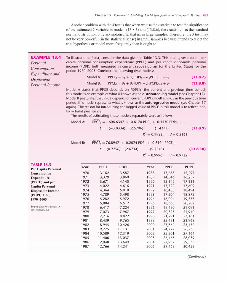
Chapter 13 Econometric Modeling: Model Specification and Diagnostic Testing 491
Another problem with the J test is that when we use the t statistic to test the significanceof the estimated Y variable in models (13.8.5) and (13.8.6), the t statistic has the standardnormal distribution only asymptotically, that is, in large samples. Therefore, the J test maynot be very powerful (in the statistical sense) in small samples because it tends to reject thetrue hypothesis or model more frequently than it ought to.
EXAMPLE 13.4PersonalConsumptionExpenditure andDisposablePersonal Income
To illustrate the J test, consider the data given in Table 13.3. This table gives data on percapita personal consumption expenditure (PPCE) and per capita disposable personalincome (PDPI), both measured in current (2008) dollars for the United States for theperiod 1970–2005. Consider the following rival models:
Model A: PPCEt = α1 + α2PDPIt + α3PDPIt−1 + ut (13.8.7)
Model B: PPCEt = β1 + β2PDPIt + β3PCPEt−1 + ut (13.8.8)
Model A states that PPCE depends on PDPI in the current and previous time period;this model is an example of what is known as the distributed-lag model (see Chapter 17).Model B postulates that PPCE depends on current PDPI as well as PPCE in the previous timeperiod; this model represents what is known as the autoregressive model (see Chapter 17again). The reason for introducing the lagged value of PPCE in this model is to reflect iner-tia or habit persistence.
The results of estimating these models separately were as follows:
Model A: PPCEt = −606.6347 + 0.6170 PDPIt + 0.3530 PDPIt−1
t = (−3.8334) (2.5706) (1.4377) (13.8.9)
R2 = 0.9983 d = 0.2161
Model B: PPCEt = 76.8947 + 0.2074 PDPIt + 0.8104 PPCEt−1
t = (0.7256) (2.6734) (9.7343) (13.8.10)
R2 = 0.9996 d = 0.9732
Year PPCE PDPI Year PPCE PDPI
1970 3,162 3,587 1988 13,685 15,2971971 3,379 3,860 1989 14,546 16,2571972 3,671 4,140 1990 15,349 17,1311973 4,022 4,616 1991 15,722 17,6091974 4,364 5,010 1992 16,485 18,4941975 4,789 5,498 1993 17,204 18,8721976 5,282 5,972 1994 18,004 19,5551977 5,804 6,517 1995 18,665 20,2871978 6,417 7,224 1996 19,490 21,0911979 7,073 7,967 1997 20,323 21,9401980 7,716 8,822 1998 21,291 23,1611981 8,439 9,765 1999 22,491 23,9681982 8,945 10,426 2000 23,862 25,4721983 9,775 11,131 2001 24,722 26,2351984 10,589 12,319 2002 25,501 27,1641985 11,406 13,037 2003 26,463 28,0391986 12,048 13,649 2004 27,937 29,5361987 12,766 14,241 2005 29,468 30,458
TABLE 13.3Per Capita PersonalConsumptionExpenditure(PPCE) and perCapita PersonalDisposable Income(PDPI), U.S.,1970–2005
Source: Economic Report ofthe President, 2007.
(Continued)
guj75772_ch13.qxd 19/08/2008 12:06 PM Page 491

492 Part Two Relaxing the Assumptions of the Classical Model
EXAMPLE 13.4(Continued)
If one were to choose between these two models on the basis of the discriminationapproach, using the highest R2 criterion, one would probably choose Model B (13.8.10)because it is just slightly higher than Model A (13.8.9). Also, in Model B (13.8.10), bothvariables are individually statistically significant, whereas in Model A (13.8.9) only thecurrent PDPI is statistically significant (there might be a collinearity problem, though). Forpredictive purposes, there is not much difference between the two estimated R2 values,though.
To apply the J test, suppose we assume Model A is the null hypothesis, or the main-tained model, and Model B is the alternative hypothesis. Following the J test stepsdiscussed earlier, we use the estimated PPCE values from model (13.8.10) as an additionalregressor in Model A. The following is the outcome from this regression:
PPCEt = −35.17 + 0.2762 PDPIt − 0.5141PDPIt−1 + 1.2351PPCEB
t
t = (−0.43) (2.60) (−4.05) (12.06) (13.8.11)
R2 = 1.00 d = 1.5205
where PPCEB
t on the right-hand side of Eq. (13.8.11) represents the estimated PPCE valuesfrom the original Model B (13.8.10). Since the coefficient of this variable is statisticallysignificant with a very high t-statistic of 12.06, following the J test procedure we have toreject Model A in favor of Model B.
Now we will assume Model B is the maintained hypothesis and Model A is the alterna-tive. Following the exact same procedure, we obtain the following results:
PPCEt = −823.7 + 1.4309 PDPIt + 1.0009 PPCEt−1 − 1.4563 PPCEA
t
t = (−3.45) (4.64) (12.06) (−4.05) (13.8.12)
R2 = 1.00 d = 1.5205
where PPCEtA on the right-hand side of Eq. (13.8.12) represents the estimated PPCE values
from the original Model A (13.8.9). In this regression, the coefficient of PPCEtA is also sta-
tistically significant with a t-statistic of −4.05. This result suggests that we should nowreject Model B in favor of Model A.
All this tells us is that neither model is particularly useful in explaining the behavior ofper capita personal consumption expenditure in the United States over the period1970–2005. Of course, we have considered only two competing models. In reality, theremay be more than two models. The J test procedure can be extended to multiple modelcomparisons, although the analysis can quickly become complex.
This example shows very vividly why the CLRM assumes that the regression modelused in the analysis is correctly specified. Obviously, in developing a model it is crucial topay very careful attention to the phenomenon being modeled.
Other Tests of Model SelectionThe J test just discussed is only one of a group of tests of model selection. There is the Coxtest, the JA test, the P test, the Mizon–Richard encompassing test, and variants of thesetests. Obviously, we cannot hope to discuss these specialized tests, for which the readermay want to consult the references cited in the various footnotes.38
38See also Badi H. Baltagi, Econometrics, Springer, New York, 1998, pp. 209–222.
guj75772_ch13.qxd 16/08/2008 03:24 PM Page 492

Chapter 13 Econometric Modeling: Model Specification and Diagnostic Testing 493
13.9 Model Selection Criteria
In this section we discuss several criteria that have been used to choose among competingmodels and/or to compare models for forecasting purposes. Here we distinguish betweenin-sample forecasting and out-of-sample forecasting. In-sample forecasting essentiallytells us how the chosen model fits the data in a given sample. Out-of-sample forecasting isconcerned with determining how a fitted model forecasts future values of the regressand,given the values of the regressors.
Several criteria are used for this purpose. In particular, we discuss these criteria: (1) R2,(2) adjusted R2( = R2), (3) Akaike’s information criterion (AIC), (4) Schwarz’s informationcriterion (SIC), (5) Mallows’s Cp criterion, and (6) forecast χ2 (chi-square). All these crite-ria aim at minimizing the residual sum of squares (RSS) (or increasing the R2 value). How-ever, except for the first criterion, criteria (2), (3), (4), and (5) impose a penalty for includingan increasingly large number of regressors. Thus there is a trade-off between goodness of fitof the model and its complexity (as judged by the number of regressors).
The R2 CriterionWe know that one of the measures of goodness of fit of a regression model is R2, which, aswe know, is defined as:
R2 = ESS
TSS= 1 − RSS
TSS(13.9.1)
R2, thus defined, of necessity lies between 0 and 1. The closer it is to 1, the better is the fit.But there are problems with R2. First, it measures in-sample goodness of fit in the sense ofhow close an estimated Y value is to its actual value in the given sample. There is no guar-antee that it will forecast well out-of-sample observations. Second, in comparing two ormore R2’s, the dependent variable, or regressand, must be the same. Third, and moreimportantly, an R2 cannot fall when more variables are added to the model. Therefore, thereis every temptation to play the game of “maximizing the R2” by simply adding more vari-ables to the model. Of course, adding more variables to the model may increase R2 but itmay also increase the variance of forecast error.
Adjusted R2
As a penalty for adding regressors to increase the R2 value, Henry Theil developed theadjusted R2, denoted by R2, which we studied in Chapter 7. Recall that
(13.9.2)
As you can see from this formula, R2 ≤ R2, showing how the adjusted R2 penalizes foradding more regressors. As we noted in Chapter 8, unlike R2, the adjusted R2 will increaseonly if the absolute t value of the added variable is greater than 1. For comparative pur-poses, therefore, R2 is a better measure than R2. But again keep in mind that the regressandmust be the same for the comparison to be valid.
R2 = 1 − RSS/(n − k)
TSS/(n − 1)= 1 − (1 − R2)
n − 1
n − k
guj75772_ch13.qxd 16/08/2008 03:24 PM Page 493

494 Part Two Relaxing the Assumptions of the Classical Model
Akaike’s Information Criterion (AIC)The idea of imposing a penalty for adding regressors to the model has been carried furtherin the AIC criterion, which is defined as:
(13.9.3)
where k is the number of regressors (including the intercept) and n is the number of obser-vations. For mathematical convenience, Eq. (13.9.3) is written as
(13.9.4)
where ln AIC = natural log of AIC and 2k/n = penalty factor. Some textbooks and soft-ware packages define AIC only in terms of its log transform so there is no need to put lnbefore AIC. As you see from this formula, AIC imposes a harsher penalty than R2 foradding more regressors. In comparing two or more models, the model with the lowest valueof AIC is preferred. One advantage of AIC is that it is useful for not only in-sample but alsoout-of-sample forecasting performance of a regression model. Also, it is useful for bothnested and non-nested models. It also has been used to determine the lag length in anAR(p) model.
Schwarz’s Information Criterion (SIC)Similar in spirit to the AIC, the SIC criterion is defined as:
(13.9.5)
or in log-form:
(13.9.6)
where [(k/n) ln n] is the penalty factor. SIC imposes a harsher penalty than AIC, as is ob-vious from comparing Eq. (13.9.6) to Eq. (13.9.4). Like AIC, the lower the value of SIC,the better the model. Again, like AIC, SIC can be used to compare in-sample or out-of-sample forecasting performance of a model.
Mallows’s Cp CriterionSuppose we have a model consisting of k regressors, including the intercept. Let σ 2 asusual be the estimator of the true σ 2. But suppose that we only choose p regressors ( p ≤ k)and obtain the RSS from the regression using these p regressors. Let RSSp denote the
ln SIC = k
nln n + ln
(RSS
n
)
SIC = nk/n
∑u2
n= nk/n RSS
n
ln AIC =(
2k
n
)+ ln
(RSS
n
)
AIC = e2k/n
∑u2
i
n= e2k/n RSS
n
guj75772_ch13.qxd 16/08/2008 03:24 PM Page 494

C p= p
Cp
p
B
A
FIGURE 13.3Mallows’s Cp plot.
Chapter 13 Econometric Modeling: Model Specification and Diagnostic Testing 495
residual sum of squares using the p regressors. Now C. P. Mallows has developed thefollowing criterion for model selection, known as the Cp criterion:
(13.9.7)
where n is the number of observations.We know that E(σ 2) is an unbiased estimator of the true σ 2. Now, if the model with p
regressors is adequate in that it does not suffer from lack of fit, it can be shown39 thatE(RSSp) = (n − p)σ 2. In consequence, it is true approximately that
E(Cp) ≈ (n − p)σ 2
σ 2− (n − 2p) ≈ p (13.9.8)
In choosing a model according to the Cp criterion, we would look for a model that has a lowCp value, about equal to p. In other words, following the principle of parsimony, we willchoose a model with p regressors ( p < k) that gives a fairly good fit to the data.
In practice, one usually plots Cp computed from Eq. (13.9.7) against p. An “adequate”model will show up as a point close to the Cp = p line, as can be seen from Figure 13.3. Asthis figure shows, Model A may be preferable to Model B, as it is closer to the Cp = p linethan Model B.
A Word of Caution about Model Selection CriteriaWe have discussed several model selection criteria. But one should look at these criteria asan adjunct to the various specification tests we have discussed in this chapter. Some of thecriteria discussed above are purely descriptive and may not have strong theoretical prop-erties. Some of them may even be open to the charge of data mining. Nonetheless, they areso frequently used by the practitioner that the reader should be aware of them. No one ofthese criteria is necessarily superior to the others.40 Most modern software packages now
Cp = RSSp
σ 2− (n − 2p)
39Norman D. Draper and Harry Smith, Applied Regression Analysis, 3d ed., John Wiley & Sons, NewYork, 1998, p. 332. See this book for some worked examples of Cp.40For a useful discussion on this topic, see Francis X. Diebold, Elements of Forecasting, 2d ed., SouthWestern Publishing, 2001, pp. 83–89. On balance, Diebold recommends the SIC criterion.
guj75772_ch13.qxd 16/08/2008 03:24 PM Page 495

496 Part Two Relaxing the Assumptions of the Classical Model
include R2, adjusted R2, AIC, and SIC. Mallows’s Cp is not routinely given, although it canbe easily computed from its definition.
Forecast Chi-Square (χ2)Suppose we have a regression model based on n observations and suppose we want to useit to forecast the (mean) values of the regressand for an additional t observations. As notedelsewhere, it is a good idea to save part of the sample data to see how the estimated modelforecasts the observations not included in the sample, the postsample period.
Now the forecast χ2 test is defined as follows:
Forecast, χ2 =∑n+t
n+1 u2i
σ 2(13.9.9)
where ui is the forecast error made for period i ( = n + 1, n + 2, . . . , + n + t), using theparameters obtained from the fitted regression and the values of the regressors in the post-sample period. σ 2 is the usual OLS estimator of σ 2 based on the fitted regression.
If we hypothesize that the parameter values have not changed between the sample andpostsample periods, it can be shown that the statistic given in Eq. (13.9.9) follows thechi-square distribution with t degrees of freedom, where t is the number of periods forwhich the forecast is made. As Charemza and Deadman note, the forecast χ2 test hasweak statistical power, meaning that the probability that the test will correctly reject afalse null hypothesis is low and therefore the test should be used as a signal rather than adefinitive test.41
13.10 Additional Topics in Econometric Modeling
As noted in the introduction to this chapter, the topic of econometric modeling and diag-nostic testing is so vast and evolving that specialized books are written on this topic. In theprevious section we have touched on some major themes in this area. In this section weconsider a few additional features that researchers may find useful in practice. In particu-lar, we consider these topics: (1) outliers, leverage, and influence; (2) recursive leastsquares; and (3) Chow’s prediction failure test. Of necessity the discussion of each ofthese topics will be brief.
Outliers, Leverage, and Influence42
Recall that, in minimizing the residual sum of squares (RSS), OLS gives equal weight toevery observation in the sample. But every observation may not have equal impact on theregression results because of the presence of three types of special data points calledoutliers, leverage, and influence points. It is important that we know what they are andhow they influence regression analysis.
In the regression context, an outlier may be defined as an observation with a “large residual.”Recall that ui = (Yi − Yi ), that is, the residual represents the difference (positive or negative)between the actual value of the regressand and its value estimated from the regression model.
41Wojciech W. Charemza and Derek F. Deadman, New Directions in Econometric Practice: A General toSpecific Modelling, Cointegration and Vector Autoregression, 2d ed., Edward Elgar Publishers, 1997,p. 30. See also pp. 250–252 for their views on various model selection criteria.42The following discussion is influenced by Chandan Mukherjee, Howard White, and Marc Wyuts,Econometrics and Data Analysis for Developing Countries, Routledge, New York, 1998, pp. 137–148.
guj75772_ch13.qxd 16/08/2008 03:24 PM Page 496

Chapter 13 Econometric Modeling: Model Specification and Diagnostic Testing 497
When we say that a residual is large, it is in comparison with the other residuals and very oftensuch a large residual catches our attention immediately because of its rather large vertical dis-tance from the estimated regression line. Note that in a data set there may be more than oneoutlier. We have already encountered an example of this in Exercise 11.22, where you wereasked to regress percent change in stock prices (Y) on percent change in consumer prices (X)for a sample of 20 countries. One observation, that relating to Chile, was an outlier.
A data point is said to exert (high) leverage if it is disproportionately distant from thebulk of the values of a regressor(s). Why does a leverage point matter? It matters be-cause it is capable of pulling the regression line toward itself, thus distorting the slope ofthe regression line. If this actually happens, then we call such a leverage (data) point aninfluential point. The removal of such a data point from the sample can dramaticallyaffect the regression line. Returning to Exercise 11.22, you will see that if you regress Yon X including the observation for Chile, the slope coefficient is positive and “highly sta-tistically significant.” But if you drop the observation for Chile, the slope coefficient ispractically zero. Thus the Chilean observation has leverage and is also an influentialobservation.
To further clarify the nature of outliers, leverage, and influence points, consider the dia-gram in Figure 13.4, which is self-explanatory.43
How do we handle such data points? Should we just drop them and confine our attentionto the remaining data points? According to Draper and Smith:
Automatic rejection of outliers is not always a wise procedure. Sometimes the outlier is pro-viding information that other data points cannot due to the fact that it arises from an unusualcombination of circumstances which may be of vital interest and requires further investigationrather than rejection. As a general rule, outliers should be rejected out of hand only if they canbe traced to causes such as errors of recording the observations or setting up the apparatus [ina physical experiment]. Otherwise, careful investigation is in order.44
Y
X
(a)
Y
X
(b)
Y
X
(c)
In each subfigure, the solid line gives the OLS line for all the data and the broken line gives theOLS line with the outlier, denoted by an , omitted. In (a), the outlier is near the mean valueof X and has low leverage and little influence on the regression coefficients. In (b), the outlieris far away from the mean value of X and has high leverage as well as substantial influence onthe regression coefficients. In (c), the outlier has high leverage but low influence on theregression coefficients because it is in line with the rest of the observations.
*
Source: Adapted from John Fox, op. cit., p. 268.
43Adapted from John Fox, Applied Regression Analysis, Linear Models, and Related Methods, SagePublications, California, 1997, p. 268.44Norman R. Draper and Harry Smith, op. cit., p. 76.
FIGURE 13.4
guj75772_ch13.qxd 16/08/2008 03:24 PM Page 497

498 Part Two Relaxing the Assumptions of the Classical Model
What are some of the tests that one can use to detect outliers and leverage points? There areseveral tests discussed in the literature, but we will not discuss them here because that willtake us far afield.45 Software packages such as SHAZAM and MICROFIT have routines todetect outliers, leverage, and influential points.
Recursive Least SquaresIn Chapter 8 we examined the question of the structural stability of a regression modelinvolving time series data and showed how the Chow test can be used for this purpose.Specifically, you may recall that in that chapter we discussed a simple savings function (sav-ings as a function of income) for the United States for the period 1970–2005. There we sawthat the savings income relationship probably changed around 1982. Knowing the point ofthe structural break we were able to confirm it with the Chow test.
But what happens if we do not know the point of the structural break (or breaks)? Thisis where one can use recursive least squares (RELS). The basic idea behind RELS is verysimple and can be explained with the savings–income regression.
Yt = β1 + β2 Xt + ut
where Y = savings and X = income and where the sample is for the period 1970–2005.(See the data in Table 8.11.)
Suppose we first use the data for 1970–1974 and estimate the savings function, obtain-ing the estimates of β1 and β2. Then we use the data for 1970–1975 and again estimate thesavings function and obtain the estimates of the two parameters. Then we use the data for1970–1976 and re-estimate the savings model. In this fashion we go on adding an addi-tional data point on Y and X until we exhaust the entire sample. As you can imagine, eachregression run will give you a new set of estimates of β1 and β2. If you plot the estimatedvalues of these parameters against each iteration, you will see how the values of estimatedparameters change. If the model under consideration is structurally stable, the changes inthe estimated values of the two parameters will be small and essentially random. However,if the estimated values of the parameters change significantly, it would indicate a structuralbreak. RELS is thus a useful routine with time series data since time is ordered chronolog-ically. It is also a useful diagnostic tool in cross-sectional data where the data are orderedby some “size” or “scale” variable, such as the employment or asset size of the firm. InExercise 13.30 you are asked to apply RELS to the savings data given in Table 8.11.
Software packages such as SHAZAM, EViews, and MICROFIT now do recursive least-squares estimates routinely. RELS also generates recursive residuals on which severaldiagnostic tests have been based.46
Chow’s Prediction Failure TestWe have already discussed Chow’s test of structural stability in Chapter 8. Chow has shownthat his test can be modified to test the predictive power of a regression model. Again, wewill revert to the U.S. savings–income regression for the period 1970–1995.
45Here are some accessible sources: Alvin C. Rencher, Linear Models in Statistics, John Wiley & Sons,New York, 2000, pp. 219–224; A. C. Atkinson, Plots, Transformations and Regression: An Introductionto Graphical Methods of Diagnostic Regression Analysis, Oxford University Press, New York, 1985,Chapter 3; Ashis Sen and Muni Srivastava, Regression Analysis: Theory, Methods, and Applications,Springer-Verlag, New York, 1990, Chapter 8; and John Fox, op. cit., Chapter 11.46For details, see Jack Johnston and John DiNardo, Econometric Methods, 4th ed., McGraw-Hill, NewYork, 1997, pp. 117–121.
guj75772_ch13.qxd 16/08/2008 03:24 PM Page 498

Chapter 13 Econometric Modeling: Model Specification and Diagnostic Testing 499
Suppose we estimate the savings–income regression for the period 1970–1981, obtain-ing β1,70−81 and β2,70−81, which are the estimated intercept and slope coefficients based onthe data for 1970–1981. Now using the actual values of income for the period 1982–1995and the intercept and slope values for the period 1970–1981, we predict the values ofsavings for each of 1982–1995 years. The logic here is that if there is no serious structuralchange in the parameter values, the values of savings estimated for 1982–1995, based onthe parameter estimates for the earlier period, should not be very different from the actualvalues of savings prevailing in the latter period. Of course, if there is a vast differencebetween the actual and predicted values of savings for the latter period, it will cast doubtson the stability of the savings–income relation for the entire data period.
Whether the difference between the actual and estimated savings value is large or smallcan be tested by the F test as follows:
F =(∑
u∗2t − ∑
u2t
)/n2(∑
u2t
)/(n1 − k)
(13.10.1)
where n1 = number of observations in the first period (1970–1981) on which the initialregression is based, n2 = number of observations in the second or forecast period,
∑u∗2
t =RSS when the equation is estimated for all the observations (n1 + n2), and
∑u2
t = RSSwhen the equation is estimated for the first n1 observations, and k is the number of para-meters estimated (two in the present instance). If the errors are independent, and identi-cally, normally distributed, the F statistic given in Eq. (13.10.1) follows the F distributionwith n2 and n1 df, respectively. In Exercise 13.31 you are asked to apply Chow’s predictivefailure test to find out if the savings–income relation has in fact changed. In passing, notethe similarity between this test and the forecast χ2 test discussed previously.
Missing DataIn applied work it is not uncommon to find that sometimes observations are missing fromthe sample data. For example, in time series data there may be gaps in the data because ofspecial circumstances. During the Second World War, data on some macro variables werenot available or were not published for strategic reasons. In cross-section data it is not un-common to find that information on some variables for some individuals is missing, espe-cially in data collected from questionnaire-type surveys. In panel data also, over time somerespondents drop out or do not provide information on all the questions.
Whatever the reason, missing data is a problem that every researcher faces from timeto time. The question is how we deal with the missing data. Is there any way to imputevalues to the missing observations?
This is not an easy question to answer. Although there are some complicated solutionssuggested in the literature, we will not pursue them here because of their complexity.47 How-ever, we will discuss two cases.48 In the first case, the reasons for the missing data are inde-pendent of the available observations, which are called by Darnell the “ignorable case.” Inthe second case, not only are the available data incomplete, but the missing observations maybe systematically related to the available data. This is a more serious case, for it may be theresult of self-selection bias, that is, the observed data are not truly randomly collected.
47For a thorough, but rather advanced, treatment of the subject, see A. Colin Cameron and Pravin K.Trivedi, Microeconometrics: Methods and Applications, Cambridge University Press, New York, 2005,Chapter 27, pp. 923–941.48The following discussion is based on Adrian C. Darnell, A Dictionary of Econometrics, Edward ElgarPublishing, Lyne, U.K., 1994, pp. 256–258.
guj75772_ch13.qxd 16/08/2008 03:24 PM Page 499

500 Part Two Relaxing the Assumptions of the Classical Model
In the ignorable case, we may simply ignore the missing observations and use the avail-able observations. Most statistical packages do this automatically. Of course, in this casethe sample size is reduced and we may not be able to get precise estimates of the regressioncoefficients. We might use the available data to shed some light on the missing observa-tions, however. Here we consider three possibilities.
1. Out of a total number of observations of N, we have complete data on N1 (N1 < N) forboth the regressand and k regressors denoted by Y1 and X1, respectively. (Y1 is vector ofN1 observations and X1 is a row vector of k regressors).
2. For some observations (N2 < N) there are complete data on the regressand, denoted byY2, but incomplete observations on some X2 (again these are vectors).
3. For some observations (N3 < N), there are no data on Y, but complete data on X, denotedby X3.
In the first case, regression of Y1 on X1 will produce estimates of the regression coefficientsthat are unbiased but they may not be efficient because we ignore N2 and N3 observations.The other two cases are rather complicated and we leave it for the reader to follow the ref-erences for solutions.49
13.11 Concluding Examples
We conclude this chapter with two examples that illustrate one or more points raised in thechapter. The first example on wage determination uses cross-section data and the secondexample, which considers the real consumption function for the U.S., uses time series data.
1. A Model of Hourly Wage Determination To examine what factors determine hourly wages, we consider a Mincer-type wage model,which has become popular with labor economists. This model has the following form:50
ln wagei = β1 + β2Edui + β3Expi + β4Fei + β5NWi + β6UNi + β7WKi + ui
(13.11.1)
Where ln wage = natural log of hourly wage ($), Edu = education in years, Exp = labormarket experience, Fe = 1 if female, 0 otherwise, NW = 1 if non-white, 0 otherwise, UN = 1if in union, 0 otherwise, and WK = 1 for non-hourly paid workers, 0 otherwise. For thenon-hourly paid workers, the hourly wage is computed as weekly earnings divided by theusual hours worked.
There are many more variables that could be added to this model. Some of these vari-ables are ethnic origin, marital status, number of children under age 6, and wealth or non-labor income. For now, we will work with the model shown in Eq. (13.11.1).
The data consist of 1,289 persons interviewed in March 1985 as a part of the CurrentPopulation Survey (CPS) periodically conducted by the U.S. Census Bureau. These datawere originally collected by Paul Rudd.51
49Besides the references already cited, see A. A. Afifi, and R. M. Elashoff, “Missing Observations inMultivariate Statistics,” Journal of the American Statistical Association, vol. 61, 1966, pp. 595–604, andvol. 62, 1967, pp. 10–29.50See J. Mincer, School, Experience and Earnings, Columbia University Press, New York, 1974.51Paul A. Rudd, An Introduction to Classical Econometric Theory, Oxford University Press, New York,2000. We have not included data on age because it is highly collinear with job experience.
guj75772_ch13.qxd 19/08/2008 12:06 PM Page 500

Chapter 13 Econometric Modeling: Model Specification and Diagnostic Testing 501
A priori, we would expect education and experience to have a positive impact on wages.The dummy variables Fe and NW are expected to have a negative impact on wages if thereis some kind of discrimination and UN is expected to have a positive impact because ofuncertainty of income.
When all the dummy variables take a value of zero, Eq. (13.11.1) reduces to
ln wagei = β1 + β2Edui + β3Expi + ui (13.11.2)
which is the wage function for a non-unionized white male worker who is on an hourlywage rate. This is the base, or reference, category.
Let us now present the regression results and then discuss them.
TABLE 13.4EViews RegressionResults Based onEquation (13.11.1)
Dependent Variable: LWMethod: Least SquaresSample: 1–1,289Included observations: 1,289
Coefficient Std. Error t Statistic Prob.
C 1.037880 0.074370 13.95563 0.0000EDU 0.084037 0.005110 16.44509 0.0000EXP 0.011152 0.001163 9.591954 0.0000FE -0.234934 0.026071 -9.011170 0.0000NW -0.124447 0.036340 -3.424498 0.0006UN 0.207508 0.036265 5.721963 0.0000WK 0.228725 0.028939 7.903647 0.0000
R-squared 0.376053 Mean dependent var. 2.342416Adjusted R-squared 0.373133 S.D. dependent var. 0.586356S.E. of regression 0.464247 Akaike info criterion 1.308614Sum squared resid. 276.3030 Schwarz criterion 1.336645Log likelihood -836.4018 Hannan-Quinn criter. 1.319136F-statistic 128.7771 Durbin-Watson stat. 1.977004Prob. (F-statistic) 0.000000
The first thing to notice is that all the estimated coefficients are individually highly signifi-cant, for the p-values are so low. The F is also very high, suggesting that collectively, also,all the variables are statistically important.
Compared to the reference worker, the average wage of a female worker and a non-whiteworker is lower. Union workers and those who are paid weekly, on average, make morewages.
How adequate is model (13.11.1), given the variables we have considered? Is it possi-ble that non-white female workers earn less than white workers? Is it possible that non-white female non-union workers earn less than white female non-union workers? In otherwords, are there any interaction effects between the quantitative regressors and the dummyvariables?
Statistical packages have routines to answer such questions. For instance, EViews hassuch a facility. After a model is estimated, if you think that some variables can be addedto the model but you are not sure of their importance, you can run the test of omittedvariables.
To show this, suppose we estimate Eq. (13.11.1) and now want to find out if the prod-ucts of Fe and NW, FE and UN, and FE and WK should be added to the model to take intoaccount the interaction between the explanatory variables. Using the EViews 6 routine, we
guj75772_ch13.qxd 16/08/2008 03:24 PM Page 501
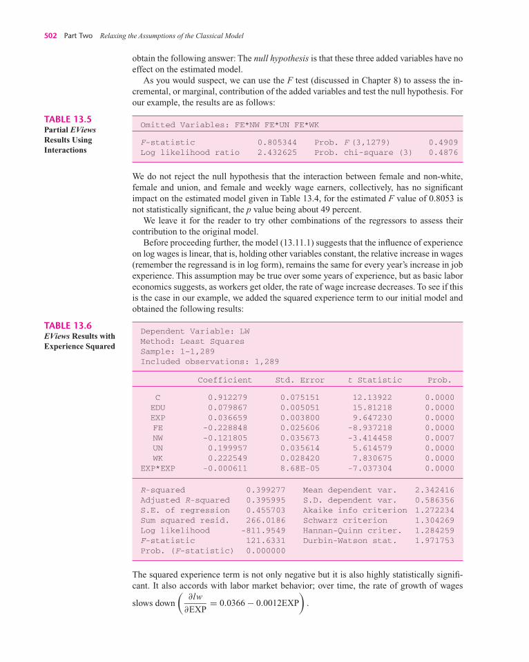
502 Part Two Relaxing the Assumptions of the Classical Model
obtain the following answer: The null hypothesis is that these three added variables have noeffect on the estimated model.
As you would suspect, we can use the F test (discussed in Chapter 8) to assess the in-cremental, or marginal, contribution of the added variables and test the null hypothesis. Forour example, the results are as follows:
TABLE 13.5Partial EViewsResults UsingInteractions
Omitted Variables: FE*NW FE*UN FE*WK
F-statistic 0.805344 Prob. F (3,1279) 0.4909Log likelihood ratio 2.432625 Prob. chi-square (3) 0.4876
We do not reject the null hypothesis that the interaction between female and non-white,female and union, and female and weekly wage earners, collectively, has no significantimpact on the estimated model given in Table 13.4, for the estimated F value of 0.8053 isnot statistically significant, the p value being about 49 percent.
We leave it for the reader to try other combinations of the regressors to assess theircontribution to the original model.
Before proceeding further, the model (13.11.1) suggests that the influence of experienceon log wages is linear, that is, holding other variables constant, the relative increase in wages(remember the regressand is in log form), remains the same for every year’s increase in jobexperience. This assumption may be true over some years of experience, but as basic laboreconomics suggests, as workers get older, the rate of wage increase decreases. To see if thisis the case in our example, we added the squared experience term to our initial model andobtained the following results:
TABLE 13.6EViews Results withExperience Squared
Dependent Variable: LWMethod: Least SquaresSample: 1–1,289Included observations: 1,289
Coefficient Std. Error t Statistic Prob.
C 0.912279 0.075151 12.13922 0.0000EDU 0.079867 0.005051 15.81218 0.0000EXP 0.036659 0.003800 9.647230 0.0000FE -0.228848 0.025606 -8.937218 0.0000NW -0.121805 0.035673 -3.414458 0.0007UN 0.199957 0.035614 5.614579 0.0000WK 0.222549 0.028420 7.830675 0.0000
EXP*EXP -0.000611 8.68E-05 -7.037304 0.0000
R-squared 0.399277 Mean dependent var. 2.342416Adjusted R-squared 0.395995 S.D. dependent var. 0.586356S.E. of regression 0.455703 Akaike info criterion 1.272234Sum squared resid. 266.0186 Schwarz criterion 1.304269Log likelihood -811.9549 Hannan-Quinn criter. 1.284259F-statistic 121.6331 Durbin-Watson stat. 1.971753Prob. (F-statistic) 0.000000
The squared experience term is not only negative but it is also highly statistically signifi-cant. It also accords with labor market behavior; over time, the rate of growth of wages
slows down
(∂lw
∂EXP= 0.0366 − 0.0012EXP
).
guj75772_ch13.qxd 16/08/2008 03:24 PM Page 502

Chapter 13 Econometric Modeling: Model Specification and Diagnostic Testing 503
We take this opportunity to discuss the Akaike and Schwarz criteria. Like R2, these aretests of the goodness of fit of the estimated model; the difference is that under the R2
criterion, the higher its value, the better the model explains the behavior of the regressand.On the other hand, under the Akaike and Schwarz criteria, the lower the value of thesestatistics, the better is the model.
Of course, all these criteria are meaningful if we want to compare two or more models.Thus, if you compare the model in Table 13.4 with the model in Table 13.6, which has theexperience-squared as an additional regressor, we see that the model in Table 13.6 is prefer-able to the one in Table 13.4 on the basis of the three criteria.
Incidentally, note that in both models the R2 values seem “low,” but such low values are typ-ically observed in cross-section data with a large number of observations. However, note thatthis “low” R2 value is statistically significant, since in both models the computed F statistic ishighly significant (recall the relationship between F and R2 discussed in Chapter 8).
Let us continue with the expanded model given in Table 13.6. Although the model lookssatisfactory, let us explore a couple of points. First, since we are dealing with cross-sectiondata, there is every chance that the model suffers from heteroscedasticity. So, we need tofind out if this is the case. We applied several of the tests of heteroscedasticity discussed inChapter 11 and found that the model does in fact suffer from heteroscedasticity. The readershould verify this assertion.
To correct for the observed heteroscedasticity, we can obtain White’s heteroscedasticity-consistent standard errors, which were discussed in Chapter 11. The results are given in thefollowing table.
TABLE 13.7EViews Results UsingWhite’s CorrectedSTD Errors
Dependent Variable: LWMethod: Least SquaresSample: 1–1,289Included observations: 1,289White’s Heteroscedasticity-Consistent Standard Errors and Covariance
Coefficient Std. Error t Statistic Prob.
C 0.912279 0.077524 11.76777 0.0000EDU 0.079867 0.005640 14.15988 0.0000EXP 0.036659 0.003789 9.675724 0.0000FE -0.228848 0.025764 -8.882625 0.0000NW -0.121805 0.033698 -3.614573 0.0003UN 0.199957 0.029985 6.668458 0.0000WK 0.222549 0.031301 7.110051 0.0000
EXP*EXP -0.000611 9.44E-05 -6.470218 0.0000
R-squared 0.399277 Mean dependent var. 2.342416Adjusted R-squared 0.395995 S.D. dependent var. 0.586356S.E. of regression 0.455703 Akaike info criterion 1.272234Sum squared resid. 266.0186 Schwarz criterion 1.304269Log likelihood -811.9549 Hannan-Quinn criter. 1.284259F-statistic 121.6331 Durbin-Watson stat. 1.971753Prob. (F-statistic) 0.000000
As you would expect, there are some changes in the estimated standard errors, althoughthis does not change the conclusion that all the regressors are important, both individuallyas well as collectively, in explaining the behavior of relative wages.
Let us now examine if the error terms are normally distributed. The histogram of theresiduals obtained from the model in Table 13.7 is shown in Figure 13.5. The Jarque–Bera
guj75772_ch13.qxd 16/08/2008 03:24 PM Page 503

504 Part Two Relaxing the Assumptions of the Classical Model
320
200
240
280
160
120
80
40
0–12.5 0.0 12.5 25.0 37.5 50.0
Series: RESIDSample: 1–1,289Observations: 1,289
Mean –9.38e-09Median –0.850280Maximum 48.92719Minimum –20.58590Std. Dev. 6.324574Skewness 1.721323Kurtosis 10.72500
Jarque–Bera 3841.617Probability 0.000000
FIGURE 13.5A histogram of theresiduals obtainedfrom the regression inTable 13.7
0–30
250 500 750 1,000 1,250
–20
–10
10
20
0
30
40
50
Estimated ln wage
RE
SID
FIGURE 13.6Residuals vs estimatedvalues of thedependent variable,ln wage
statistic rejects the hypothesis that the errors are normally distributed, for the JB statisticis high and the p value is practically zero: Note that for a normally distributed variable, theskewness and kurtosis coefficients are, respectively, 0 and 3.
Now what? Our hypothesis testing procedure thus far has rested on the assumption that thedisturbance, or error, term in the regression model is normally distributed. Does this meanthat we cannot legitimately use the t and F tests to test hypotheses in our wage regression?
The answer is no. As noted in the chapter, the OLS estimators are asymptotically normallydistributed with the caveat noted in the chapter, namely that the error term has finite variance,is homoscedastic, and the mean value of the error term, given the values of the explanatoryvariables, is zero. As a result, we can continue to use the usual t and F tests, provided thesample is reasonably large. In passing it may be noted that we did not need the normalityassumption to obtain OLS estimators. Even without the normality assumption the OLS esti-mators are best linear unbiased estimators (BLUE) under the Gauss–Markov assumptions.
How large is a large sample? There is no definitive answer to this question, but the sam-ple size of 1,289 observations in our wage regression seems reasonably large.
Are there any “outliers” in our wage regression? Some idea about this can be gleanedfrom the graph in Figure 13.6, which gives the actual and estimated values of the dependent
guj75772_ch13.qxd 19/08/2008 06:34 PM Page 504

Chapter 13 Econometric Modeling: Model Specification and Diagnostic Testing 505
TABLE 13.8Sample: 1–1,289
W EDU EXP
Mean 12.36585 13.14507 18.78976Median 10.08000 12.00000 18.00000Maximum 64.08000 20.00000 56.00000Minimum 0.840000 0.000000 0.000000Std. Dev. 7.896350 2.813823 11.66284Skewness 1.848114 -0.290381 0.375669Kurtosis 7.836565 5.977464 2.327946
Jarque–Bera 1990.134 494.2552 54.57664Probability 0.000000 0.000000 0.000000
Sum 15939.58 16944.00 24220.00Sum Sq. Dev. 80309.82 10197.87 175196.0
Observations 1,289 1,289 1,289
variable (ln wage) and the residuals, which are the differences between the actual and es-timated values of the regressand.
Although the mean value of the residuals is always zero (why?), the graph in Figure 13.6shows that there are several residuals that seem large (in absolute value) compared with thebulk of the residuals. It is possible that there are outliers in the data. We provide the rawstatistics on the three quantitative variables in Table 13.8 to aid the reader in decidingwhether there are indeed outliers.
TABLE 13.9Results of RegressionEquation (13.11.3)
Method: Least SquaresSample: 1947–2000Included observations: 54
Coefficient Std. Error t Statistic Prob.
C -0.467711 0.042778 -10.93343 0.0000LOG(YD) 0.804873 0.017498 45.99836 0.0000
LOG(WEALTH) 0.201270 0.017593 11.44060 0.0000INTEREST -0.002689 0.000762 -3.529265 0.0009
R-squared 0.999560 Mean dependent var. 7.826093Adjusted R-squared 0.999533 S.D. dependent var. 0.552368S.E. of regression 0.011934 Akaike info criterion -5.947703Sum squared resid. 0.007121 Schwarz criterion -5.800371Log likelihood 164.5880 Hannan-Quinn criter. -5.890883F-statistc 37832.59 Durbin-Watson stat. 1.289219Prob. (F-statistic) 0.000000
2. Real Consumption Function for the United States, 1947–2000In Chapter 10 we considered the consumption function for the U.S. for the years 1947–2000.The specific form of the consumption function we considered was:
ln TCt = β1 + β2 ln YDt + β3 ln W + β4Interestt + ut (13.11.3)
Where TC, YD, W, and Interest are, respectively, total consumption expenditure, personaldisposable income, wealth, and interest rate, all in real terms. The results based on our dataare as follows:
guj75772_ch13.qxd 19/08/2008 06:34 PM Page 505

506 Part Two Relaxing the Assumptions of the Classical Model
Since TC, YD, and Wealth enter in logarithmic form, the estimated slope coefficients of YDand Wealth are, respectively, income and wealth elasticities. As you would expect, theseelasticities are positive and are highly statistically significant. Numerically, the income andwealth elasticities are about 0.80 and 0.20. The coefficient of the interest rate variablerepresents semielasticity (why?). Holding other variables constant, the results show that ifthe interest rate goes up by 1 percentage point, on average, real consumption expendituregoes down by about 0.27 percent. Note that the estimated semielasticity is also highlystatistically significant.
Look at some of the summary statistics. The R2 value is very high, almost reaching100 percent. The F value is also highly statistically significant, suggesting that, not onlyindividually, but also collectively, all the explanatory variables have a significant impact onconsumption expenditure.
The Durbin–Watson statistic, however, suggests that errors in the model are serially cor-related. If we consult the Durbin–Watson tables (Table D.5 in Appendix D), we see that for55 observations (the closest number to 54) and three explanatory variables, the lower andupper 5 percent critical d values are 1.452 and 1.681. Since the observed d in our example,1.2892, is below the lower critical d values, we may conclude that the errors in our con-sumption function are positively correlated. This should not be a surprising finding, formost time series regressions suffer from autocorrelation.
But before we accept this conclusion, let us find out if there are any specification errors.As we know, sometimes autocorrelation may be apparent because we have omittedsome important variables. To see if this is the case, we consider the regression obtained inTable 13.10.
TABLE 13.10Dependent Variable: LTCMethod: Least SquaresSample: 1947–2000Included observations: 54
Coefficient Std. Error t Statistic Prob.
C 2.689644 0.566034 4.751737 0.0000LYD 0.512836 0.054056 9.487076 0.0000LW -0.205281 0.074068 -2.771510 0.0079
INTEREST -0.001162 0.000661 -1.759143 0.0848LYD*LW 0.039901 0.007141 5.587986 0.0000
R-squared 0.999731 Mean dependent var. 7.826093Adjusted R-squared 0.999709 S.D. dependent var. 0.552368S.E. of regression 0.009421 Akaike info criterion -6.403689Sum squared resid. 0.004349 Schwarz criterion -6.219524Log likelihood 177.8996 Hannan-Quinn criter. -6.332663F-statistic 45534.94 Durbin-Watson Stat. 1.530268Prob. (F-statistic) 0.000000
The additional variable in this model is the interaction of the logs of disposable incomeand wealth. This interaction term is highly significant. Notice that now the interest variablehas become less significant ( p value of about 8 percent), although it retains its negative sign.But now the Durbin–Watson d value has increased from about 1.28 to about 1.53.
The 5 percent critical d values now are 1.378 and 1.721. The observed d value of 1.53lies between these values, suggesting that, on the basis of the Durbin–Watson statistic, wecannot determine whether or not we have autocorrelation. However, the observed d value is
guj75772_ch13.qxd 16/08/2008 03:24 PM Page 506

Chapter 13 Econometric Modeling: Model Specification and Diagnostic Testing 507
closer to the upper limit d value. As noted in the chapter on autocorrelation, some authorssuggest using the upper limit of the d statistic as approximately the true significance limit;therefore, if the computed d value is below the upper limit, there is evidence of positive au-tocorrelation. By that criterion, in the present instance we can conclude that our model suf-fers from positive autocorrelation.
We also applied the Breusch–Godfrey test of autocorrelation that we discussed in Chap-ter 12. Adding the two lagged terms of the estimated residuals in Equation (12.6.15) to themodel in Table 13.9, we obtained the following results:
TABLE 13.11Breusch–Godfrey Serial Correlation LM Test:
F-statistic 3.254131 Prob. F(2,48) 0.0473Obs*R-squared 6.447576 Prob. chi-square (2) 0.0398
Dependent Variable: RESIDMethod: Least SquaresSample: 1947–2000Included observations: 54Presample missing value lagged residuals set to zero.
Coefficient Std. Error t Statistic Prob.
C -0.006514 0.041528 -0.156851 0.8760LYD -0.004197 0.017158 -0.244619 0.8078LW 0.004191 0.017271 0.242674 0.8093
INTEREST 0.000116 0.000736 0.156964 0.8759RESID(-1) 0.385190 0.151581 2.541147 0.0143RESID(-2) -0.165609 0.154695 -1.070556 0.2897
R-squared 0.119400 Mean dependent var. -9.02E-17Adjusted R-squared 0.027670 S.D. dependent var. 0.011591S.E. of regression 0.011430 Akaike info criterion -6.000781Sum squared resid. 0.006271 Schwarz criterion -5.779782Log likelihood 168.0211 Hannan-Quinn criter. -5.915550F-statistic 1.301653 Durbin-Watson Stat. 1.848014Prob. (F-statistic) 0.279040
The F reported at the top tests the hypothesis that the two lagged residuals included in themodel have zero values. This hypothesis is rejected because the F is significant at about the5 percent level.
To sum up, it seems that there is autocorrelation in the error term. We can apply one ormore procedures discussed in Chapter 12 to remove autocorrelation. But to save space, weleave that task to the reader.
In Table 13.12 we report the results of regression analysis that present the HAC orNewey–West standard errors that take into account the autocorrelation. Our sample size of54 observations is large enough to use the HAC standard errors.
If you compare these results with those given in Table 13.9, you will observe that theregression coefficients remain the same, but that the standard errors are somewhat different.
In this chapter we discussed Chow’s prediction failure test. We have a sample period thatextends from 1947 to 2000. Over this period, we have had several business cycles, mostlyof short durations. For example, there was a recession in 1990 and another one in 2000. Is
guj75772_ch13.qxd 16/08/2008 03:24 PM Page 507

508 Part Two Relaxing the Assumptions of the Classical Model
TABLE 13.13Chow’s Test ofPredictive Failure
Chow’s Forecast Test: Forecast from 1991 to 2000
F-statistic 1.957745 Prob. F (10,40) 0.0652Log likelihood ratio 21.51348 Prob. chi-square (10) 0.0178
Dependent Variable: LTCMethod: Least SquaresSample: 1947–1990Included observations: 44
Coefficient Std. Error t Statistic Prob.
C -0.287952 0.095089 -3.028236 0.0043LYD 0.853172 0.028473 29.96474 0.0000LW 0.141513 0.033085 4.277239 0.0001
INTEREST -0.002060 0.000804 -2.562790 0.0143
R-squared 0.999496 Mean dependent var. 7.659729Adjusted R-squared 0.999458 S.D. dependent var. 0.469580S.E. of regression 0.010933 Akaike info criterion -6.107640Sum squared resid. 0.004781 Schwarz criterion -5.945441Log likelihood 138.3681 Hannan-Quinn criter. -6.047489F-statistic 26430.49 Durbin-Watson Stat. 1.262748Prob. (F-statistic) 0.000000
TABLE 13.12Dependent Variable: LTCMethod: Least SquaresSample: 1947–2000Included observations: 54Newey–West HAC Standard Errors and Covariance (lag truncation = 3)
Coefficient Std. Error t Statistic Prob.
C -0.467714 0.043937 -10.64516 0.0000LYD 0.804871 0.017117 47.02132 0.0000LW 0.201272 0.015447 13.02988 0.0000
INTEREST -0.002689 0.000880 -3.056306 0.0036
R-squared 0.999560 Mean dependent var. 7.826093Adjusted R-squared 0.999533 S.D. dependent var. 0.552368S.E. of regression 0.011934 Akaike info criterion -5.947707Sum squared resid. 0.007121 Schwarz criterion -5.800374Log likelihood 164.5881 Hannan-Quinn criter. -5.890886F-statistic 37832.71 Durbin-Watson Stat. 1.289237Prob. (F-statistic) 0.000000
the behavior of consumer expenditure in relation to income, wealth, and the interest ratedifferent during recessions?
To shed light on this question, let us consider the 1990 recession and apply Chow’s predic-tion failure test. The details of this test have already been discussed in the chapter. UsingChow’s predictive failure test in EViews, version 6, we obtain the results given in Table 13.13.
guj75772_ch13.qxd 16/08/2008 03:24 PM Page 508

Chapter 13 Econometric Modeling: Model Specification and Diagnostic Testing 509
Apparently, it seems that the consumption function pre- and post-1990 are statisticallydifferent, for the computed F statistic, following Eq. (8.7.4), is highly statistically signifi-cant because the p value is only 0.0052.
The reader is encouraged to apply Chow’s parameter stability and predictive failure teststo determine if the consumption function pre- and post-2000 has changed. To do this, youwill have to extend the data beyond 2000. Also note that to apply these tests the number ofobservations must be greater than the number of coefficients estimated.
We have exhausted all of the diagnostic tests that we can apply to our consumption data.But the analysis provided thus far should give you a fairly good idea about how one canapply the various tests.
13.12 Non-Normal Errors and Stochastic Regressors
In this section we discuss two topics that are of a somewhat advanced nature, namely,non-normal distribution of the error term, and stochastic, or random, regressors and theirpractical importance.
1. What Happens If the Error Term Is Not Normally Distributed?In the classical normal linear regression model (CNLRM) discussed in Chapter 4, weassumed that the error term u follows the normal distribution. We invoked the central limittheorem (CLT) to justify the normality assumption. Because of this assumption, we wereable to establish that the OLS estimators are also normally distributed. As a result, we wereable to do hypothesis testing using the t and F tests regardless of the sample size. We alsodiscussed using the Jarque–Bera and Anderson–Darling normality tests to find out if theestimated errors are normally distributed in any practical application.
What happens if the errors are not normally distributed? It can be stated that the OLSestimators are still BLUE, that is, they are unbiased and in the class of linear estimatorsthey show minimum variance. Intuitively, this should not be surprising, for to establish theGauss–Markov (BLUE) theorem we did not need the normality assumption.
Then what is the problem?The problem is that we need the sampling, or probability, distributions of the OLS
estimators.Without that we cannot engage in any kind of hypothesis testing regarding the truevalues of these estimators. As shown in Chapters 3 and 7, the OLS estimators are linear
TABLE 13.14Chow’s Test ofParameter Stability
Chow Breakpoint Test: 1990Null Hypothesis: No breaks at specified breakpointsVarying regressors: All equation variablesEquation Sample: 1947–2000
F-statistic 4.254054 Prob. F(4,46) 0.0052Log likelihood ratio 16.99654 Prob. chi-square (4) 0.0019Wald statistic 17.01622 Prob. chi-square (4) 0.0019
The F statistic given in the top portion of Table 13.13 suggests that there probably is nota substantial difference in the consumption function pre- and post-1990, for its p value isnot significant at the 5 percent level. But if you choose the 10 percent level of significance,the F value is statistically significant.
We can look at this problem differently. In Chapter 8 we discussed a test of parameterstability. To see if there has been any statistically significant change in the consumptionfunction regression coefficients, we used the Chow test discussed in Section 8.7 of Chapter 8and obtained the results given in Table 13.14.
guj75772_ch13.qxd 16/08/2008 03:24 PM Page 509

510 Part Two Relaxing the Assumptions of the Classical Model
funtions of the dependent variable Y, and Y itself is a linear function of the stochastic errorterm u, assuming that the explanatory variables are non-stochastic, or fixed in repeatedsampling. Ultimately, then, we need the probability distribution of u.
As noted above, the classical normal linear regression model (CNLRM) assumes thatthe error term follows the normal distribution (with zero mean and constant variance).Using the central limit theorem (CLT) to justify the normality of the error term, we wereable to show that the OLS estimators themselves are normally distributed with means andvariance discussed in Chapters 4 and 7. This in turn allowed us to use the t and F statisticsin hypothesis testing in small, or finite, samples as well as in large samples. Therefore, therole of the normality assumption is very critical, especially in small samples.
But what if we cannot maintain the normality assumption on the basis of various nor-mality tests? What then? We have two choices. The first is bootstrapping and the second isto invoke large, or asymptotic, sample theory.
A discussion of bootstrapping, which is gradually seeping into applied econometrics,will take us far afield. The basic idea underlying bootstrapping is to churn (or regurgitate)a given sample over and over again and then obtain the sampling distributions of the para-meters of interest (OLS estimators for our purpose). How this is done in practice is best leftfor references.52 By the way, the term bootstrapping comes from the commonly used ex-pression, “to pull oneself up by one’s own bootstrap.”
The other approach to deal with non-normal error terms is to use asymptotic, or largesample theory. As a matter of fact, a glimpse of this was given in Appendix 3A.7 in Chap-ter 3, where we showed that the OLS estimators are consistent.As discussed in AppendixA,an estimator is consistent if it approaches the true value of the estimator as the sample sizegets larger and larger (see Figure A.11 in Appendix A).
But how does that help us in hypothesis testing? Can we still use the t and F tests? It canbe shown that under the Gauss–Markov assumptions the OLS estimators are asymptoticallynormally distributed with the means and variances discussed in Chapters 4 and 7.53 As aresult, the t and F tests developed under the normality assumption are approximately validin large samples. The approximation becomes quite good as the sample size increases.54
2. Stochastic Explanatory VariablesIn Chapter 3 we introduced the classical linear (in parameter) regression model under somesimplifying assumptions. One of the assumptions was that the explanatory variables, orregressors, were either fixed or non-stochastic, or if stochastic, they were independent ofthe error term. We called the former case the fixed regressor case and the latter the randomregressor case.
52For an informal discussion, see Christopher Z. Mooney and Robert D. Duval, Bootstrapping: A Nonparametric Approach to Statistical Inference, Sage University Press, California, 1993. For a more formal textbook discussion, see Russell Davidson and James G. MacKinnon, Econometric Theory andMethods, Oxford University Press, New York, 2004, pp. 159–166.53Recall the Gauss–Markov assumptions, namely, the expected value of the error term is zero, the error term and each of the explanatory variables are independent, the error variance ishomoscedastic, and there is no autocorrelation in the error term. It is also assumed that the variance-covariance matrix of the explanatory variables is finite. We can also relax the condition ofindependence between the error term and the regressors and assume the weaker condition that theyare uncorrelated.54The proof of asymptotic normality of OLS estimators is beyond the scope of this book. See James H.Stock and Mark W. Watson, Introduction to Econometrics, 2d ed., Pearson/Addison Wesley, Boston,2007, pp. 710–711.
guj75772_ch13.qxd 16/08/2008 03:24 PM Page 510

Chapter 13 Econometric Modeling: Model Specification and Diagnostic Testing 511
In the fixed regressor case, we already know the properties of the OLS estimators (seeChapters 5 and 8). In the random regressor case, if we proceed with the assumption that ouranalysis is conditional on the given values of the regressors, the properties of OLS estima-tors that we have studied under the fixed regressor case continue to hold true.
If in the random regressor case we assume that these regressors and the error term areindependently distributed, the OLS estimators are still unbiased but they are no longerefficient.55
Things get complicated if the error term is not normally distributed, or regressors arestochastic, or both. Here it is difficult to make any general statements regarding the finite-sample properties of the OLS estimators. However, under certain conditions, we can invokethe central limit theorem to establish the asymptotic normality of OLS estimators. Althoughbeyond the scope of this book, the proofs can be found elsewhere.56
13.13 A Word to the Practitioner
We have covered a lot of ground in this chapter. There is no question that model building isan art as well as a science. A practical researcher may be bewildered by theoretical nicetiesand an array of diagnostic tools. But it is well to keep in mind Martin Feldstein’s cautionthat “The applied econometrician, like the theorist, soon discovers from experience that auseful model is not one that is ‘true’ or ‘realistic’ but one that is parsimonious, plausibleand informative.”57
Peter Kennedy of Simon Fraser University in Canada advocates the following “TenCommandments of Applied Econometrics”:58
1. Thou shalt use common sense and economic theory.
2. Thou shalt ask the right questions (i.e., put relevance before mathematical elegance).
3. Thou shalt know the context (do not perform ignorant statistical analysis).
4. Thou shalt inspect the data.
5. Thou shalt not worship complexity. Use the KISS principle, that is, keep it stochasti-cally simple.
6. Thou shalt look long and hard at thy results.
7. Thou shalt beware the costs of data mining.
8. Thou shalt be willing to compromise (do not worship textbook prescriptions).
9. Thou shalt not confuse significance with substance (do not confuse statistical signifi-cance with practical significance).
10. Thou shalt confess in the presence of sensitivity (that is, anticipate criticism).
You may want to read Kennedy’s paper fully to appreciate the conviction with which headvocates the above ten commandments. Some of these commandments may soundtongue-in-cheek, but there is a grain of truth in each.
55For technical details, see William H. Greene, Econometric Analysis, 6th ed., Pearson/Prentice-Hall,New Jersey, 2008, pp. 49–50.56See Greene, op. cit.57Martin S. Feldstein, “Inflation, Tax Rules and Investment: Some Econometric Evidence,” Econometrica, vol. 30, 1982, p. 829.58Peter Kennedy, op. cit., pp. 17–18.
guj75772_ch13.qxd 16/08/2008 03:24 PM Page 511

512 Part Two Relaxing the Assumptions of the Classical Model
1. The assumption of the CLRM that the econometric model used in analysis is correctlyspecified has two meanings. One, there are no equation specification errors, and two,there are no model specification errors. In this chapter the major focus was on equationspecification errors.
2. The equation specification errors discussed in this chapter were (1) omission of an im-portant variable(s), (2) inclusion of a superfluous variable(s), (3) adoption of thewrong function form, (4) incorrect specification of the error term ui, and (5) errors ofmeasurement in the regressand and regressors.
3. When legitimate variables are omitted from a model, the consequences can be veryserious: The OLS estimators of the variables retained in the model are not only bi-ased but inconsistent as well. Additionally, the variances and standard errors ofthese coefficients are incorrectly estimated, thereby vitiating the usual hypothesis-testing procedures.
4. The consequences of including irrelevant variables in the model are fortunately lessserious: The estimators of the coefficients of the relevant as well as “irrelevant” vari-ables remain unbiased as well as consistent, and the error variance σ 2 remains cor-rectly estimated. The only problem is that the estimated variances tend to be larger thannecessary, thereby making for less precise estimation of the parameters. That is, theconfidence intervals tend to be larger than necessary.
5. To detect equation specification errors, we considered several tests, such as (1) exam-ination of residuals, (2) the Durbin–Watson d statistic, (3) Ramsey’s RESET test, and(4) the Lagrange multiplier test.
6. A special kind of specification error is errors of measurement in the values of theregressand and regressors. If there are errors of measurement in the regressand only,the OLS estimators are unbiased as well as consistent but they are less efficient. Ifthere are errors of measurement in the regressors, the OLS estimators are biased aswell as inconsistent.
7. Even if errors of measurement are detected or suspected, the remedies are often noteasy. The use of instrumental or proxy variables is theoretically attractive but notalways practical. Thus it is very important in practice that the researcher be careful instating the sources of his/her data, how they were collected, what definitions were used,etc. Data collected by official agencies often come with several footnotes and theresearcher should bring those to the attention of the reader.
8. Model mis-specification errors can be as serious as equation specification errors. Inparticular, we distinguished between nested and non-nested models. To decide on theappropriate model we discussed the non-nested, or encompassing, F test and theDavidson–MacKinnon J test and pointed out the limitations of each test.
9. In choosing an empirical model in practice researchers have used a variety of criteria.We discussed some of these, such as the Akaike and Schwarz information criteria,Mallows’s Cp criterion, and forecast χ2 criterion. We discussed the advantages anddisadvantages of these criteria and also warned the reader that these criteria are notabsolute but are adjunct to a careful specification analysis.
10. We also discussed these additional topics: (1) outliers, leverage, and influence; (2) recursive least squares; and (3) Chow’s prediction failure test. We discussed therole of each in applied work.
11. We discussed briefly two special cases, namely, non-normality of the stochastic error termand random regressors and the role of asymptotic, or large, sample theory in situationswhere small, or finite, sample properties of OLS estimators canot be established.
Summary andConclusions
guj75772_ch13.qxd 16/08/2008 03:24 PM Page 512

Chapter 13 Econometric Modeling: Model Specification and Diagnostic Testing 513
12. We concluded this chapter by discussing Peter Kennedy’s “ten commandments ofapplied econometrics.” The point of these commandments is to ask the researcher tolook beyond the purely technical aspects of econometrics.
Questions13.1. Refer to the demand function for chicken estimated in Eq. (8.6.23). Considering the
attributes of a good model discussed in Section 13.1, could you say that this de-mand function is “correctly” specified?
13.2. Suppose that the true model is
Yi = β1 Xi + ui (1)
but instead of fitting this regression through the origin you routinely fit the usualintercept-present model:
Yi = α0 + α1 Xi + vi (2)
Assess the consequences of this specification error.
13.3. Continue with Exercise 13.2 but assume that it is model (2) that is the truth. Discussthe consequences of fitting the mis-specified model (1).
13.4. Suppose that the “true” model is
Yi = β1 + β2 X2i + ut (1)
but we add an “irrelevant” variable X3 to the model (irrelevant in the sense that thetrue β3 coefficient attached to the variable X3 is zero) and estimate
Yi = β1 + β2 X2i + β3 X3i + vi (2)
a. Would the R2 and the adjusted R2 for model (2) be larger than that for model (1)?
b. Are the estimates of β1 and β2 obtained from model (2) unbiased?
c. Does the inclusion of the “irrelevant” variable X3 affect the variances of β1 and β2?
13.5. Consider the following “true” (Cobb–Douglas) production function:
ln Yi = α0 + α1 ln L1i + α2 ln L2i + α3 ln Ki + ui
where Y = outputL1 = production laborL2 = nonproduction laborK = capital
But suppose the regression actually used in empirical investigation is
ln Yi = β0 + β1 ln L1i + β2 ln Ki + ui
On the assumption that you have cross-sectional data on the relevant variables,
a. Will E(β1) = α1 and E(β2) = α3?
b. Will the answer in (a) hold if it is known that L2 is an irrelevant input in the pro-duction function? Show the necessary derivations.
13.6. Refer to Eqs. (13.3.4) and (13.3.5). As you can see, α2, although biased, has asmaller variance than β2, which is unbiased. How would you decide on the trade-off
EXERCISES
guj75772_ch13.qxd 16/08/2008 03:24 PM Page 513

514 Part Two Relaxing the Assumptions of the Classical Model
between bias and smaller variance? Hint: The MSE (mean-square error) for the twoestimators is expressed as
MSE(α2) =(σ 2
/∑x2
2i
)+ β2
3 b23 2
= sampling variance + square of bias
MSE(β2) = σ 2/∑
x22
(1 − r2
2 3
)
On MSE, see Appendix A.
13.7. Show that β estimated from either Eq. (13.5.1) or Eq. (13.5.3) provides an unbiasedestimate of true β.
13.8. Following Friedman’s permanent income hypothesis, we may write
Y ∗i = α + βX∗
i (1)
where Y ∗i = “permanent” consumption expenditure and X∗
i = “permanent” income.Instead of observing the “permanent” variables, we observe
Yi = Y ∗i + ui
Xi = X∗i + vi
where Yi and Xi are the quantities that can be observed or measured and where ui
and vi are measurement errors in Y ∗ and X∗, respectively.Using the observable quantities, we can write the consumption function as
Yi = α + β(Xi − vi ) + ui
= α + βXi + (ui − βvi ) (2)
Assuming that (1) E(ui ) = E(vi ) = 0, (2) var (ui ) = σ 2u and var (vi ) = σ 2
v ,(3) cov (Y ∗
i , ui ) = 0, cov (X∗i, vi ) = 0, and (4) cov (ui, X∗
i ) = cov (vi, Y ∗i ) =
cov(ui, vi ) = 0, show that in large samplesβestimated from Eq. (2) can be expressed as
plim (β) = β
1 + (σ 2
v /σ 2X∗
)a. What can you say about the nature of the bias in β?
b. If the sample size increases indefinitely, will the estimated β tend toward equal-ity with the true β?
13.9. Capital asset pricing model. The capital asset pricing model (CAPM) of moderninvestment theory postulates the following relationship between the average rate ofreturn of a security (common stock), measured over a certain period, and the volatil-ity of the security, called the beta coefficient (volatility is measure of risk):
Ri = α1 + α2(βi ) + ui (1)
where R i = average rate of return of security i
βi = true beta coefficient of security i
ui = stochastic disturbance term
The true βi is not directly observable but is measured as follows:
rit = α1 + β∗rmt + et (2)
guj75772_ch13.qxd 16/08/2008 03:24 PM Page 514

Chapter 13 Econometric Modeling: Model Specification and Diagnostic Testing 515
where rit = rate of return of security i for time t
rmt = market rate of return for time t (this rate is the rate of return on somebroad market index, such as the S&P index of industrial securities)
et = residual term
and where β∗ is an estimate of the “true” beta coefficient. In practice, therefore,instead of estimating Eq. (1), one estimates
Ri = α1 + α2(β∗i ) + ui (3)
where β∗i are obtained from the regression (2). But since β∗
i are estimated, the rela-tionship between true β and β∗ can be written as
β∗i = βi + vi (4)
where vi can be called the error of measurement.
a. What will be the effect of this error of measurement on the estimate of α2?
b. Will the α2 estimated from Eq. (3) provide an unbiased estimate of true α2? If not,is it a consistent estimate of α2? If not, what remedial measures do you suggest?
13.10. Consider the model
Yi = β1 + β2 X2i + ui (1)
To find out whether this model is mis-specified because it omits the variable X3
from the model, you decide to regress the residuals obtained from model (1) on thevariable X3 only. (Note: There is an intercept in this regression.) The Lagrange mul-tiplier (LM) test, however, requires you to regress the residuals from model (1) onboth X2 and X3 and a constant. Why is your procedure likely to be inappropriate?*
13.11. Consider the model
Yi = β1 + β2 X∗i + ui
In practice we measure X∗i by Xi such that
a. Xi = X∗i + 5
b. Xi = 3X∗i
c. Xi = (X∗i + εi ), where εi is a purely random term with the usual properties
What will be the effect of these measurement errors on estimates of true β1 and β2?
13.12. Refer to the regression Eqs. (13.3.1) and (13.3.2). In a manner similar to Eq. (13.3.3)show that
E(α1) = β1 + β3( X3 − b32 X2)
where b3 2 is the slope coefficient in the regression of the omitted variable X3 on theincluded variable X2.
13.13. Critically evaluate the following view expressed by Leamer:†
My interest in metastatistics [i.e., theory of inference actually drawn from data] stemsfrom my observations of economists at work. The opinion that econometric theory is
*See Maddala, op. cit., p. 477.†Edward E. Leamer, Specification Searches: Ad Hoc Inference with Nonexperimental Data, John Wiley &Sons, New York, 1978, p. vi.
guj75772_ch13.qxd 16/08/2008 03:24 PM Page 515

516 Part Two Relaxing the Assumptions of the Classical Model
irrelevant is held by an embarrassingly large share of the economic profession. Thewide gap between econometric theory and econometric practice might be expected tocause professional tension. In fact, a calm equilibrium permeates our journals and our[professional] meetings. We comfortably divide ourselves into a celibate priesthood ofstatistical theorists, on the one hand, and a legion of inveterate sinner-data analysts, onthe other. The priests are empowered to draw up lists of sins and are revered for thespecial talents they display. Sinners are not expected to avoid sins; they need only con-fess their errors openly.
13.14. Evaluate the following statement made by Henry Theil:*
Given the present state of the art, the most sensible procedure is to interpret confi-dence coefficients and significance limits liberally when confidence intervals andtest statistics are computed from the final regression of a regression strategy in theconventional way. That is, a 95 percent confidence coefficient may actually be an80 percent confidence coefficient and a 1 percent significance level may actually be a10 percent level.
13.15. Commenting on the econometric methodology practiced in the 1950s and early1960s, Blaug stated:†
. . . much of it [i.e., empirical research] is like playing tennis with the net down:instead of attempting to refute testable predictions, modern economists all too fre-quently are satisfied to demonstrate that the real world conforms to their predictions,thus replacing falsification [à la Popper], which is difficult, with verification, whichis easy.
Do you agree with this view? You may want to peruse Blaug’s book to learn moreabout his views.
13.16. According to Blaug, “There is no logic of proof but there is logic of disproof.”‡
What does he mean by this?
13.17. Refer to the St. Louis model discussed in the text. Keeping in mind the problemsassociated with the nested F test, critically evaluate the results presented in regres-sion (13.8.4).
13.18. Suppose the true model is
Yi = β1 + β2 Xi + β2 X2i + β3 X3
i + ui
but you estimate
Yi = α1 + α2 Xi + vi
If you use observations of Y at X = −3, −2, −1, 0, 1, 2, 3, and estimate the“incorrect” model, what bias will result in these estimates?§
13.19. To see if the variable X2i belongs in the model Yi = β1 + β2 Xi + ui , Ramsey’s
RESET test would estimate the linear model, obtaining the estimated Yi values fromthis model [i.e., Yi = β1 + β2 Xi ] and then estimating the model Yi = α1 + α2 Xi+α3Y 2
i + vi and testing the significance of α3. Prove that, if α3 turns out to be statisti-cally significant in the preceding (RESET) equation, it is the same thing as estimating
*Henry Theil, Principles of Econometrics, John Wiley & Sons, New York, 1971, pp. 605–606.†M. Blaug, The Methodology of Economics. Or How Economists Explain, Cambridge University Press,New York, 1980, p. 256.‡Ibid., p. 14.§Adapted from G. A. F., Sebeir, Linear Regression Analysis, John Wiley & Sons, New York, 1977, p. 176.
guj75772_ch13.qxd 16/08/2008 03:24 PM Page 516

Chapter 13 Econometric Modeling: Model Specification and Diagnostic Testing 517
the following model directly: Yi = β1 + β2 Xi + β3 X2i + ui . (Hint: Substitute for
Yi in the RESET regression.)*
13.20. State with reason whether the following statements are true or false.†
a. An observation can be influential but not an outlier.
b. An observation can be an outlier but not influential.
c. An observation can be both influential and an outlier.
d. If in the model Yi = β1 + β2 Xi + β3 X2i + ui β3 turns out to be statistically
significant, we should retain the linear term Xi even if β2 is statisticallyinsignificant.
e. If you estimate the model Yi = β1 + β2 X2i + β3 X3i + ui or Yi = α1 + β2x2i+β3x3i + ui by OLS, the estimated regression line is the same, where x2i =(X2i − X2) and x3i = (X3i − X3).
Empirical Exercises
*Adapted from Kerry Peterson, op. cit., pp. 184–185.†Adapted from Norman R. Draper and Harry Smith, op. cit., pp. 606–607.
13.21. Use the data for the demand for chicken given in Exercise 7.19. Suppose you aretold that the true demand function is
ln Yt = β1 + β2 ln X2t + β3 ln X3t + β6 ln X6t + ut (1)
but you think differently and estimate the following demand function:
ln Yt = α1 + α2 ln X2t + α3 ln X3t + vt (2)
where Y = per capita consumption of chickens (lb)
X2 = real disposable per capita income
X3 = real retail price of chickens
X6 = composite real price of chicken substitutes
a. Carry out RESET and LM tests of specification errors, assuming the demandfunction (1) just given is the truth.
b. Suppose β6 in Eq. (1) turns out to be statistically insignificant. Does that meanthere is no specification error if we fit Eq. (2) to the data?
c. If β6 turns out to be insignificant, does that mean one should not introduce theprice of a substitute product(s) as an argument in the demand function?
13.22. Continue with Exercise 13.21. Strictly for pedagogical purposes, assume thatmodel (2) is the true demand function.
a. If we now estimate model (1), what type of specification error is committed inthis instance?
b. What are the theoretical consequences of this specification error? Illustrate withthe data at hand.
13.23. The true model is
Y ∗i = β1 + β2 X∗
i + ui (1)
but because of errors of measurement you estimate
Yi = α1 + α2 Xi + vi (2)
where Yi = Y ∗i + εi and Xi = X∗
i + wi , where εi and wi are measurement errors.
guj75772_ch13.qxd 16/08/2008 03:24 PM Page 517

518 Part Two Relaxing the Assumptions of the Classical Model
Using the data given in Table 13.2, document the consequences of estimatingmodel (2) instead of the true model (1).
13.24. Monte Carlo experiment.* Ten individuals had weekly permanent income as fol-lows: $200, 220, 240, 260, 280, 300, 320, 340, 380, and 400. Permanent consump-tion (Y ∗
i ) was related to permanent income X∗i as
Y ∗i = 0.8X∗
i (1)
Each of these individuals had transitory income equal to 100 times a random num-ber ui drawn from a normal population with mean = 0 and σ 2 = 1 (i.e., standardnormal variable). Assume that there is no transitory component in consumption.Thus, measured consumption and permanent consumption are the same.
a. Draw 10 random numbers from a normal population with zero mean and unitvariance and obtain 10 numbers for measured income Xi ( = X∗
i + 100ui ).
b. Regress permanent ( = measured) consumption on measured income using thedata obtained in (a) and compare your results with those shown in Eq. (1). Apriori, the intercept should be zero (why?). Is that the case? Why or why not?
c. Repeat (a) 100 times and obtain 100 regressions as shown in (b) and compareyour results with the true regression (1). What general conclusions do you draw?
13.25. Refer to Exercise 8.26. With the definitions of the variables given there, considerthe following two models to explain Y:
Model A: Yt = α1 + α2 X3t + α3 X4t + α4 X6t + ut
Model B: Yt = β1 + β2 X2t + β3 X5t + β4 X6t + ut
Using the nested F test, how will you choose between the two models?
13.26. Continue with Exercise 13.25. Using the J test, how would you decide between thetwo models?
13.27. Refer to Exercise 7.19, which is concerned with the demand for chicken in theUnited States. There you were given five models.
a. What is the difference between model 1 and model 2? If model 2 is correct andyou estimate model 1, what kind of error is committed? Which test would youapply—equation specification error or model selection error? Show the neces-sary calculations.
b. Between models 1 and 5, which would you choose? Which test(s) do you useand why?
13.28. Refer to Table 8.11, which gives data on personal savings (Y) and personal dispos-able income (X) for the period 1970–2005. Now consider the following models:
Model A: Yt = α1 + α2 Xt + α3 Xt−1 + ut
Model B: Yt = β1 + β2 Xt + β3Yt−1 + ut
How would you choose between these two models? State clearly the test proce-dure(s) you use and show all the calculations. Suppose someone contends that theinterest rate variable belongs in the savings function. How would you test this?Collect data on the 3-month treasury bill rate as a proxy for the interest and demon-strate your answer.
*Adapted from Christopher Dougherty, Introduction to Econometrics, Oxford University Press, New York, 1992, pp. 253–256.
guj75772_ch13.qxd 19/08/2008 06:34 PM Page 518

Chapter 13 Econometric Modeling: Model Specification and Diagnostic Testing 519
*This can be generalized to the case where more than one relevant X variable is excluded from themodel. On this, see Chandan Mukherjee et al., op. cit., p. 215.
13.29. Use the data in Exercise 13.28.To familiarize yourself with recursive least squares, es-timate the savings functions for 1970–1981, 1970–1985, 1970–1990, and 1970–1995.Comment on the stability of estimated coefficients in the savings functions.
13.30. Continue with Exercise 13.29, but now use the updated data in Table 8.10.
a. Suppose you estimate the savings function for 1970–1981. Using the parametersthus estimated and the personal disposable income data from 1982–2000, esti-mate the predicted savings for the latter period and use Chow’s prediction failuretest to find out if it rejects the hypothesis that the savings function between thetwo time periods has not changed.
b. Now estimate the savings function for the data from 2000–2005. Compare theresults to the function for the 1982–2000 period using the same method as above(Chow’s prediction failure test). Is there a significant change in the savings func-tion between the two periods?
13.31. Omission of a variable in the K-variable regression model. Refer to Eq. (13.3.3),which shows the bias in omitting the variable X3 from the model Yi = β1+β2 X2i + β3 X3i + ui . This can be generalized as follows: In the k-variable modelYi = β1 + β2 X2i + · · · + βk Xki + ui , suppose we omit the variable Xk . Then it canbe shown that the omitted variable bias of the slope coefficient of included variableXj is:
E(βj ) = βj + βkbk j j = 2, 3, . . . , (k − 1)
where bkj is the (partial) slope coefficient of Xj in the auxiliary regression of theexcluded variable Xk on all the explanatory variables included in the model.*
Refer to Exercise 13.21. Find out the bias of the coefficients in Eq. (1) if weexcluded the variable ln X6 from the model. Is this exclusion serious? Show thenecessary calculations.
Appendix 13A
13A.1 The Proof that E(b12) = β2 + β3b32[Equation (13.3.3)]
In the deviation form the three-variable population regression model can be written as
yi = β2x2i + β3x3i + (ui − u) (1)
First multiplying by x2 and then by x3, the usual normal equations are
∑yi x2i = β2
∑x2
2i + β3
∑x2i x3i +
∑x2i (ui − u) (2)
∑yi x3i = β2
∑x2i x3i + β3
∑x2
3i +∑
x3i (ui − u) (3)
Dividing Eq. (2) by ∑
x22i on both sides, we obtain
∑yi x2i∑x2
2i
= β2 + β3
∑x2i x3i∑
x22i
+∑
x2i (ui − u)∑x2
2i
(4)
guj75772_ch13.qxd 16/08/2008 03:24 PM Page 519

520 Part Two Relaxing the Assumptions of the Classical Model
Now recalling that
b1 2 =∑
yi x2i∑x2
2i
b3 2 =∑
x2i x3i∑x2
2i
Eq. (4) can be written as
b1 2 = β2 + β3b3 2 +∑
x2i (ui − u)∑x2
2i
(5)
Taking the expected value of Eq. (5) on both sides, we finally obtain
E(b1 2) = β2 + β3b3 2 (6)
where use is made of the facts that (a) for a given sample, b3 2 is a known fixed quantity, (b) β2 andβ3 are constants, and (c) ui is uncorrelated with X2i (as well as X3i ).
13A.2 The Consequences of Including an IrrelevantVariable: The Unbiasedness Property
For the true model (13.3.6), we have
β2 =∑
yx2∑x2
2
(1)
and we know that it is unbiased.For the model (13.3.7), we obtain
α2 =(∑
yx2
)(∑x2
3
)−
(∑yx3
)(∑x2x3
)∑
x22
∑x2
3 −(∑
x2x3
)2 (2)
Now the true model in deviation form is
yi = β2x2 + (ui − u) (3)
Substituting for yi from model (3) into model (2) and simplifying, we obtain
E(α2) = β2
∑x2
2
∑x2
3 −(∑
x2x3
)2
∑x2
2
∑x2
3 −(∑
x2x3
)2
= β2
(4)
that is, α2 remains unbiased.We also obtain
α3 =(∑
yx3
)(∑x2
2
)−
(∑yx2
)(∑x2x3
)∑
x22
∑x2
3 −(∑
x2x3
)2 (5)
guj75772_ch13.qxd 16/08/2008 03:24 PM Page 520

Chapter 13 Econometric Modeling: Model Specification and Diagnostic Testing 521
Substituting for yi from model (3) into model (5) and simplifying, we obtain
E(α3) = β2
[(∑x2x3
)(∑x2
2
)−
(∑x2x3
)(∑x2
2
)]∑
x22
∑x2
3 −(∑
x2x3
)2
= 0
(6)
which is its value in the true model since X3 is absent from the true model.
13A.3 The Proof of Equation (13.5.10)
We have
Y = α + βX∗i + ui (1)
Xi = X∗i + wi (2)
Therefore, in deviation form we obtain
yi = βx∗i + (ui − u) (3)
xi = x∗i + (wi − w) (4)
Now when we use
Yi = α + βXi + ui (5)
we obtain
β =∑
yx∑x2
=∑
[βx∗ + (u − u)][x∗ + (w − w)]∑[x∗ + (w − w)]2
using (3) and (4)
= β∑
x∗2 + β∑
x∗(w − w) + ∑x∗(u − u) + ∑
(u − u)(w − w)∑x∗2 + 2
∑x∗(w − w) + ∑
(w − w)2
Since we cannot take expectation of this expression because the expectation of the ratio of twovariables is not equal to the ratio of their expectations (note: the expectations operator E is a linearoperator), first we divide each term of the numerator and the denominator by n and take the proba-bility limit, plim (see Appendix A for details of plim), of
β = (1/n)[β
∑x∗2 + β
∑x∗(w − w) + ∑
x∗(u − u) + ∑(u − u)(w − w)
](1/n)
[∑x∗2 + 2
∑x∗(w − w) + ∑
(w − w)2]
Now the probability limit of the ratio of two variables is the ratio of their probability limits. Applyingthis rule and taking plim of each term, we obtain
plim β = βσ 2X∗
σ 2X∗ + σ 2
w
where σ 2X∗ and σ 2
w are variances of X∗ and w as sample size increases indefinitely and where we haveused the fact that as the sample size increases indefinitely there is no correlation between the errors uand w as well as between them and the true X∗. From the preceding expression, we finally obtain
plim β = β
1
1 +(σ 2
w
/σ 2
X∗)
which is the required result.
guj75772_ch13.qxd 16/08/2008 03:24 PM Page 521

522 Part Two Relaxing the Assumptions of the Classical Model
13A.4 The Proof of Equation (13.6.2)
Since there is no intercept in the model, the estimate of α, according to the formula for the regressionthrough the origin, is as follows:
α =∑
Xi Yi∑X2
i
(1)
Substituting for Y from the true model (13.2.8), we obtain
α =∑
Xi (βXi u i )∑X2
i
= β
∑X2
i u i∑X2
i
(2)
Statistical theory shows that if ln ui ∼ N (0, σ 2) then
ui = log normal[eσ 2/2, eσ 2
(eσ 2−1
)](3)
Therefore,
E(α) = βE
∑X2
i u i∑X2
i
= β
E
(X2
1u1 + X22u2 + · · · + X2
nun
)∑
X2i
= βeσ 2/2
∑X2
i∑X2
i
= βeσ 2/2
where use is made of the fact that the X ’s are nonstochastic and each ui has an expected value ofeσ 2/2.
Since E(α) �= β, α is a biased estimator of β .
guj75772_ch13.qxd 16/08/2008 03:24 PM Page 522

In Part 1 we introduced the classical linear regression model with all its assumptions.In Part 2 we examined in detail the consequences that ensue when one or more of theassumptions are not satisfied and what can be done about them. In Part 3 we study someselected but commonly encountered econometric techniques. In particular, we discussthese topics: (1) nonlinear-in-the-parameter regression models, (2) qualitative responseregression models, (3) panel data regression models, and (4) dynamic econometricmodels.
In Chapter 14, we consider models that are intrinsically nonlinear in the parameters.With the ready availability of software packages, it is no longer a big challenge to estimatesuch models. Although the underlying mathematics may elude some readers, the basicideas of nonlinear-in-the-parameter regression models can be explained intuitively. Withsuitable examples, this chapter shows how such models are estimated and interpreted.
In Chapter 15, we consider regression models in which the dependent variable is qualita-tive in nature. This chapter therefore complements Chapter 9, where we discussed models inwhich the explanatory variables were qualitative in nature. The basic thrust of this chapter ison developing models in which the regressand is of the yes or no type. Since ordinary leastsquares (OLS) poses several problems in estimating such models, several alternatives havebeen developed. In this chapter we consider two such alternatives, namely, the logit modeland the probit model. This chapter also discusses several variants of the qualitative responsemodels, such as the Tobit model and the Poisson regression model. Several extensions ofthe qualitative response models are also briefly discussed, such as the ordered probit,ordered logit, and multinomial logit.
In Chapter 16 we discuss panel data regression models. Such models combine timeseries and cross-section observations. Although by combining such observations we increasethe sample size, panel data regression models pose several estimation challenges. In thischapter we discuss only the essentials of such models and guide the reader to the appropriateresources for further study.
Part3Topics inEconometrics
guj75772_ch14.qxd 16/08/2008 04:48 PM Page 523

524 Part Three Topics in Econometrics
In Chapter 17, we consider regression models that include current as well as past, orlagged, values of the explanatory variables in addition to models that include the laggedvalue(s) of the dependent variable as one of the explanatory variables. These models arecalled, respectively, distributed lag and autoregressive models. Although such models areextremely useful in empirical econometrics, they pose some special estimating problemsbecause they violate one or more assumptions of the classical regression model. We con-sider these special problems in the context of the Koyck, the adaptive-expectations (AE),and the partial-adjustment models. We also note the criticism leveled against the AE modelby the advocates of the so-called rational expectations (RE) school.
guj75772_ch14.qxd 16/08/2008 04:48 PM Page 524

525
Chapter 14NonlinearRegression ModelsThe major emphasis of this book is on linear regression models, that is, models that arelinear in the parameters and/or models that can be transformed so that they are linear inthe parameters. On occasions, however, for theoretical or empirical reasons we have toconsider models that are nonlinear in the parameters.1 In this chapter we take a look atsuch models and study their special features.
14.1 Intrinsically Linear and IntrinsicallyNonlinear Regression Models
When we started our discussion of linear regression models in Chapter 2, we stated that ourconcern in this book is basically with models that are linear in the parameters; they may ormay not be linear in the variables. If you refer to Table 2.3, you will see that a model that islinear in the parameters as well as the variables is a linear regression model and so is amodel that is linear in the parameters but nonlinear in the variables. On the other hand, if amodel is nonlinear in the parameters it is a nonlinear (in-the-parameter) regression modelwhether the variables of such a model are linear or not.
However, one has to be careful here, for some models look nonlinear in the parametersbut are inherently or intrinsically linear because with suitable transformation they can bemade linear-in-the-parameter regression models. But if such models cannot be linearized inthe parameters, they are called intrinsically nonlinear regression models. From now onwhen we talk about a nonlinear regression model, we mean that it is intrinsically nonlinear.For brevity, we will call them NLRM.
To drive home the distinction between the two, let us revisit Exercises 2.6 and 2.7. In Ex-ercise 2.6, Models a, b, c, and e are linear regression models because they are all linear inthe parameters. Model d is a mixed bag, for β2 is linear but not ln β1. But if we letα = ln β1, then this model is linear in α and β2.
In Exercise 2.7, Models d and e are intrinsically nonlinear because there is no simple wayto linearize them. Model c is obviously a linear regression model. What about Models a
1We noted in Chapter 4 that under the assumption of normally distributed error term, the OLS esti-mators are not only BLUE but are BUE (best unbiased estimator) in the entire class of estimators,linear or not. But if we drop the assumption of normality, as Davidson and MacKinnon note, it ispossible to obtain nonlinear and/or biased estimators that may perform better than the OLS estima-tors. See Russell Davidson and James G. MacKinnon, Estimation and Inference in Econometrics, OxfordUniversity Press, New York, 1993, p. 161.
guj75772_ch14.qxd 16/08/2008 04:48 PM Page 525

526 Part Three Topics in Econometrics
and b? Taking the logarithms on both sides of a, we obtain ln Yi = β1 + β2 Xi + ui , which islinear in the parameters. Hence Model a is intrinsically a linear regression model. Model bis an example of the logistic (probability) distribution function, and we will study this inChapter 15. On the surface, it seems that this is a nonlinear regression model. But a simplemathematical trick will render it a linear regression model, namely,
ln
(1 − Yi
Yi
)= β1 + β2 Xi + ui (14.1.1)
Therefore, Model b is intrinsically linear. We will see the utility of models like Eq. (14.1.1)in the next chapter.
Consider now the famous Cobb–Douglas (C–D) production function. LettingY = output, X2 = labor input, and X3 = capital input, we will write this function in threedifferent ways:
Yi = β1 Xβ2
2i Xβ3
3i eui (14.1.2)
or,
ln Yi = α + β2 ln X2i + β3 ln X3i + ui (14.1.2a)
where α = ln β1. Thus in this format the C–D function is intrinsically linear.Now consider this version of the C–D function:
Yi = β1 Xβ2
2i Xβ3
3i ui (14.1.3)
or,
ln Yi = α + β2 ln X2i + β3 ln X3i + ln ui (14.1.3a)
where α = ln β1. This model too is linear in the parameters.But now consider the following version of the C–D function:
Yi = β1 Xβ2
2i Xβ3
3i + ui (14.1.4)
As we just noted, C–D versions (14.1.2a) and (14.1.3a) are intrinsically linear (in the para-meter) regression models, but there is no way to transform Eq. (14.1.4) so that the trans-formed model can be made linear in the parameters.2 Therefore, Eq. (14.1.4) is intrinsicallya nonlinear regression model.
Another well-known but intrinsically nonlinear function is the constant elasticity ofsubstitution (CES) production function of which the Cobb–Douglas production is a spe-cial case. The CES production takes the following form:
Yi = A[δK −β
i + (1 − δ)L−β
i
]−1/β (14.1.5)
where Y = output, K = capital input, L = labor input, A = scale parameter,δ = distribution parameter (0 < δ < 1), and β = substitution parameter (β ≥ −1).3 Nomatter in what form you enter the stochastic error term ui in this production function, thereis no way to make it a linear (in parameter) regression model. It is intrinsically a nonlinearregression model.
2If you try to log-transform the model, it will not work because ln (A + B ) �= ln A + ln B .3For properties of the CES production function, see Michael D. Intriligator, Ronald Bodkin, and ChengHsiao, Econometric Models, Techniques, and Applications, 2d ed., Prentice Hall, 1996, pp. 294–295.
guj75772_ch14.qxd 16/08/2008 04:48 PM Page 526

Chapter 14 Nonlinear Regression Models 527
14.2 Estimation of Linear and Nonlinear Regression Models
To see the difference in estimating linear and nonlinear regression models, consider the fol-lowing two models:
Yi = β1 + β2 Xi + ui (14.2.1)
Yi = β1eβ2 Xi + ui (14.2.2)
By now you know that Eq. (14.2.1) is a linear regression model, whereas Eq. (14.2.2) is anonlinear regression model. Regression (14.2.2) is known as the exponential regressionmodel and is often used to measure the growth of a variable, such as population, GDP, ormoney supply.
Suppose we consider estimating the parameters of the two models by ordinary leastsquares (OLS). In OLS we minimize the residual sum of squares (RSS), which for model(14.2.1) is: ∑
u2i =
∑(Yi − β1 − β2 Xi )
2(14.2.3)
where as usual β1 and β2 are the OLS estimators of the true β’s. Differentiating the preced-ing expression with respect to the two unknowns, we obtain the normal equations shown inEqs. (3.1.4) and (3.1.5). Solving these equations simultaneously, we obtain the OLS estima-tors given in Eqs. (3.1.6) and (3.1.7). Observe very carefully that in these equations theunknowns (β’s) are on the left-hand side and the knowns (X and Y) are on the right-handside. As a result we get explicit solutions of the two unknowns in terms of our data.
Now see what happens if we try to minimize the RSS of Eq. (14.2.2). As shown inAppendix 14A, Section 14A.1, the normal equations corresponding to Eqs. (3.1.4) and(3.1.5) are as follows:
∑Yi e
β2 Xi = β1e2β2 Xi (14.2.4)∑
Yi Xi eβ2 Xi = β1
∑Xi e
2β2 Xi (14.2.5)
Unlike the normal equations in the case of the linear regression model, the normal equa-tions for nonlinear regression have the unknowns (the β’s) both on the left- and right-handsides of the equations. As a consequence, we cannot obtain explicit solutions of the un-knowns in terms of the known quantities. To put it differently, the unknowns are expressedin terms of themselves and the data! Therefore, although we can apply the method of leastsquares to estimate the parameters of the nonlinear regression models, we cannot obtainexplicit solutions of the unknowns. Incidentally, OLS applied to a nonlinear regressionmodel is called nonlinear least squares (NLLS). So, what is the solution? We take thisquestion up next.
14.3 Estimating Nonlinear Regression Models: The Trial-and-Error Method
To set the stage, let us consider a concrete example. The data in Table 14.1 relates to themanagement fees that a leading mutual fund in the United States pays to its investment ad-visors to manage its assets. The fees paid depend on the net asset value of the fund. As youcan see, the higher the net asset value of the fund, the lower are the advisory fees, which canbe seen clearly from Figure 14.1.
guj75772_ch14.qxd 16/08/2008 04:48 PM Page 527

528 Part Three Topics in Econometrics
To see how the exponential regression model in Eq. (14.2.2) fits the data given in Table14.1, we can proceed by trial and error. Suppose we assume that initially β1 = 0.45 andβ2 = 0.01. These are pure guesses, sometimes based on prior experience or prior empiricalwork or obtained by just fitting a linear regression model even though it may not be appro-priate. At this stage do not worry about how these values are obtained.
Since we know the values of β1 and β2, we can write Eq. (14.2.2) as:
ui = Yi − β1eβ2 Xi = Yi − 0.45e0.01Xi (14.3.1)
Therefore, ∑u2
i =∑
(Yi − 0.45e0.01Xi )2 (14.3.2)
Since Y, X, β1, and β2 are known, we can easily find the error sum of squares in Eq. (14.3.2).4
Remember that in OLS our objective is to find those values of the unknown parameters thatwill make the error sum of squares as small as possible. This will happen if the estimated
00.36
10 20 30 40
Asset, billions of dollars
50 60 70
0.40
0.44
0.48
Fee
, %
0.52
0.56FIGURE 14.1Relationship ofadvisory fees to fundassets.
TABLE 14.1Advisory FeesCharged and AssetSize
Fee, % Asset*
1 0.520 0.52 0.508 5.03 0.484 104 0.46 155 0.4398 206 0.4238 257 0.4115 308 0.402 359 0.3944 40
10 0.388 4511 0.3825 5512 0.3738 60
*Asset represents net asset value, billions of dollars.
4Note that we call ∑
u2i the error sum of squares and not the usual residual sum of squares because
the values of the parameters are assumed to be known.
guj75772_ch14.qxd 16/08/2008 04:48 PM Page 528

Chapter 14 Nonlinear Regression Models 529
Y values from the model are as close as possible to the actual Y values. With the givenvalues, we obtain
∑u2
i = 0.3044. But how do we know that this is the least possible errorsum of squares that we can obtain? What happens if you choose another value for β1 andβ2, say, 0.50 and −0.01, respectively? Repeating the procedure just laid down, we find thatwe now obtain
∑u2
i = 0.0073. Obviously, this error sum of squares is much smaller thanthe one obtained before, namely, 0.3044. But how do we know that we have reached thelowest possible error sum of squares, if by choosing yet another set of values for the β’s, wewill obtain yet another error sum of squares?
As you can see, such a trial-and-error, or iterative, process can be easily implemented.And if one has infinite time and infinite patience, the trial-and-error process may ultimatelyproduce values of β1 and β2 that may guarantee the lowest possible error sum of squares. Butyou might ask, how did we go from (β1 = 0.45; β2 = 0.01) to (β1 = 0.50; β2 = −0.01)?Clearly, we need some kind of algorithm that will tell us how we go from one set of valuesof the unknowns to another set before we stop. Fortunately such algorithms are available,and we discuss them in the next section.
14.4 Approaches to Estimating Nonlinear Regression Models
There are several approaches, or algorithms, to NLRMs: (1) direct search or trial and error,(2) direct optimization, and (3) iterative linearization.5
Direct Search or Trial-and-Error or Derivative-Free MethodIn the previous section we showed how this method works. Although intuitively appealingbecause it does not require the use of calculus methods as the other methods do, thismethod is generally not used. First, if an NLRM involves several parameters, the methodbecomes very cumbersome and computationally expensive. For example, if an NLRM in-volves 5 parameters and 25 alternative values for each parameter are considered, you willhave to compute the error sum of squares (25)5 = 9,765,625 times! Second, there is noguarantee that the final set of parameter values you have selected will necessarily give youthe absolute minimum error sum of squares. In the language of calculus, you may obtain alocal and not an absolute minimum. In fact, no method guarantees a global minimum.
Direct OptimizationIn direct optimization we differentiate the error sum of squares with respect to each unknowncoefficient, or parameter, set the resulting equation to zero, and solve the resulting normalequations simultaneously. We have already seen this in Eqs. (14.2.4) and (14.2.5). But as youcan see from these equations, they cannot be solved explicitly or analytically. Some iterativeroutine is therefore called for. One routine is called the method of steepest descent. We willnot discuss the technical details of this method as they are somewhat involved, but the readercan find the details in the references. Like the method of trial and error, the method of steepestdescent also involves selecting initial trial values of the unknown parameters but then it pro-ceeds more systematically than the hit-or-miss or trial-and-error method. One disadvantage ofthis method is that it may converge to the final values of the parameters extremely slowly.
5The following discussion leans heavily on these sources: Robert S. Pindyck and Daniel L. Rubinfeld,Econometric Models and Economic Forecasts, 4th ed., McGraw-Hill, 1998, Chapter 10; Norman R.Draper and Harry Smith, Applied Regression Analysis, 3d ed., John Wiley & Sons, 1998, Chapter 24;Arthur S. Goldberger, A Course in Econometrics, Harvard University Press, 1991, Chapter 29; RussellDavidson and James MacKinnon, op. cit., pp. 201–207; John Fox, Applied Regression Analysis, LinearModels, and Related Methods, Sage Publications, 1997, pp. 393–400; and Ronald Gallant, NonlinearStatistical Models, John Wiley and Sons, 1987.
guj75772_ch14.qxd 03/09/2008 11:05 AM Page 529

530 Part Three Topics in Econometrics
Iterative Linearization MethodIn this method we linearize a nonlinear equation around some initial values of the parame-ters. The linearized equation is then estimated by OLS and the initially chosen values areadjusted. These adjusted values are used to relinearize the model, and again we estimate itby OLS and readjust the estimated values. This process is continued until there is no sub-stantial change in the estimated values from the last couple of iterations. The main tech-nique used in linearizing a nonlinear equation is the Taylor series expansion fromcalculus. Rudimentary details of this method are given in Appendix 14A, Section 14A.2.Estimating NLRM using Taylor series expansion is systematized in two algorithms, knownas the Gauss–Newton iterative method and the Newton–Raphson iterative method.Since one or both of these methods are now incorporated in several computer packages,and since a discussion of their technical details will take us far beyond the scope of thisbook, there is no need to dwell on them here.6 In the next section we discuss some exam-ples using these methods.
14.5 Illustrative Examples
6There is another method that is sometimes used, called the Marquard method, which is a com-promise between the method of steepest descent and the linearization (or Taylor series) method. Theinterested reader may consult the references for the details of this method.7EViews provides three options: quadratic hill climbing, Newton–Raphson, and Berndt–Hall–Hall–Hausman. The default option is quadratic hill climbing, which is a variation of the Newton–Raphson method.
EXAMPLE 14.1Mutual FundAdvisory Fees
Refer to the data given in Table 14.1 and the NLRM (14.2.2). Using the EViews 6 nonlinearregression routine, which uses the linearization method,7 we obtained the followingregression results; the coefficients, their standard errors, and their t values are given in atabular form:
Variable Coefficient Std. Error t Value p Value
Intercept 0.5089 0.0074 68.2246 0.0000Asset −0.0059 0.00048 −12.3150 0.0000
R 2 = 0.9385 d = 0.3493
From these results, we can write the estimated model as:
Feei = 0.5089 Asset−0.0059 (14.5.1)
Before we discuss these results, it may be noted that if you do not supply the initial valuesof the parameters to start the linearization process, EViews will do it on its own. It tookEViews five iterations to obtain the results shown in Eq. (14.5.1). However, you can supplyyour own initial values to start the process. To demonstrate, we chose the initial value ofβ1 = 0.45 and β2 = 0.01. We obtained the same results as in Eq. (14.5.1) but it took eightiterations. It is important to note that fewer iterations will be required if your initial values arenot very far from the final values. In some cases you can choose the initial values of theparameters by simply running an OLS regression of the regressand on the regressor(s),simply ignoring the nonlinearities. For instance, using the data in Table 14.1, if you wereto regress fee on assets, the OLS estimate of β1 is 0.5028 and that of β2 is −0.002, which
guj75772_ch14.qxd 19/08/2008 06:46 PM Page 530

Chapter 14 Nonlinear Regression Models 531
are much closer to the final values given in Eq. (14.5.1). (For the technical details, seeAppendix 14A, Section 14A.3.)
Now about the properties of nonlinear least squares (NLLS) estimators. You may recallthat, in the case of linear regression models with normally distributed error terms, we wereable to develop exact inference procedures (i.e., test hypotheses) using the t, F, and χ2
tests in small as well as large samples. Unfortunately, this is not the case with NLRMs, evenwith normally distributed error terms. The NLLS estimators are not normally distributed, arenot unbiased, and do not have minimum variance in finite, or small, samples. As a result, wecannot use the t test (to test the significance of an individual coefficient) or the F test (totest the overall significance of the estimated regression) because we cannot obtain anunbiased estimate of the error variance σ 2 from the estimated residuals. Furthermore, theresiduals (the difference between the actual Y values and the estimated Y values from theNLRM) do not necessarily sum to zero, ESS and RSS do not necessarily add up to the TSS,and therefore R 2 = ESS/TSS may not be a meaningful descriptive statistic for such mod-els. However, we can compute R 2 as:
R 2 = 1 −∑
u2i∑
(Y i − Y )2(14.5.2)
where Y = regressand and u i = Yi − Y i , where Y i are the estimated Y values from the(fitted) NLRM.
Consequently, inferences about the regression parameters in nonlinear regression areusually based on large-sample theory. This theory tells us that the least-squares and max-imum likelihood estimators for nonlinear regression models with normal error terms,when the sample size is large, are approximately normally distributed and almost unbi-ased, and have almost minimum variance. This large-sample theory also applies when theerror terms are not normally distributed.8
In short, then, all inference procedures in NLRM are large sample, or asymptotic.Returning to Example 14.1, the t statistics given in Eq. (14.5.1) are meaningful only ifinterpreted in the large-sample context. In that sense, we can say that estimated coeffi-cients shown in Eq. (14.5.1) are individually statistically significant. Of course, our sample inthe present instance is rather small.
Returning to Eq. (14.5.1), how do we find out the rate of change of Y ( = fee) with re-spect to X (asset size)? Using the basic rules of derivatives, the reader can see that the rateof change of Y with respect to X is:
dYdX
= β1β2e β2 X = (−0.0059)(0.5089)e−0.0059X (14.5.3)
As can be seen, the rate of change of fee depends on the value of the assets. Forexample, if X = 20 (million), the expected rate of change in the fees charged can beseen from Eq. (14.5.3) to be about −0.0031 percent. Of course, this answer willchange depending on the X value used in the computation. Judged by the R2 as com-puted from Eq. (14.5.2), the R2 value of 0.9385 suggests that the chosen NLRM fits thedata in Table 14.1 quite well. The estimated Durbin–Watson value of 0.3493 may sug-gest that there is autocorrelation or possibly model specification error. Although thereare procedures to take care of these problems as well as the problem of heteroscedas-ticity in NLRM, we will not pursue these topics here. The interested reader may consultthe references.
8John Neter, Michael H. Kutner, Christopher J. Nachtsheim, and William Wasserman, Applied Regres-sion Analysis, 3d ed., Irwin, 1996, pp. 548–549.
EXAMPLE 14.1(Continued)
guj75772_ch14.qxd 19/08/2008 12:46 PM Page 531

532 Part Three Topics in Econometrics
EXAMPLE 14.2The Cobb–DouglasProductionFunction of the MexicanEconomy
Refer to the data given in Exercise 14.9 (Table 14.3). These data refer to the Mexican econ-omy for years 1955–1974. We will see if the NLRM given in Eq. (14.1.4) fits the data, not-ing that Y = output, X2 = labor input, and X3 = capital input. Using EViews 6, we obtainedthe following regression results, after 32 iterations.
Variable Coefficient Std. Error t Value p Value
Intercept 0.5292 0.2712 1.9511 0.0677Labor 0.1810 0.1412 1.2814 0.2173Capital 0.8827 0.0708 12.4658 0.0000
R 2 = 0.9942 d = 0.2899
Therefore, the estimated Cobb–Douglas production function is:
GDPt = 0.5292Labor0.1810t Capital0.8827
t (14.5.4)
Interpreted asymptotically, the equation shows that only the coefficient of the capital input issignificant in this model. In Exercise 14.9 you are asked to compare these results with thoseobtained from the multiplicative Cobb–Douglas production function as given in Eq. (14.1.2).
EXAMPLE 14.3Growth of U.S.Population,1970–2007
The Table in Exercise 14.8 gives data on total U.S. population for the period 1970–2007.A logistic model of the following type is often used to measure the growth of somepopulations, human beings, bacteria, etc.:
Yt = β1
1 + e (β2+βt3)
+ ut (14.5.5)
Where Y = population, in millions; t = time, measured chronologically; and the β’s are theparameters.
This model is nonlinear in the parameters; there is no simple way to convert it into a modelthat is linear in the parameters. So we will need to use one of the nonlinear estimation meth-ods to estimate the parameters. Notice an interesting feature of this model: Although thereare only two variables in the model, population and time, there are three unknown parame-ters, which shows that in a NLRM there can be more parameters than variables.
An attempt to fit Eq. (14.5.5) to our data was not successful, as all the estimated coef-ficients were statistically insignificant. This is probably not surprising, for if we plot popu-lation against time, we obtain Figure 14.2.
1970
1972
1974
1976
1978
1980
1982
1984
1986
1988
1990
1992
1994
1996
1998
2000
2002
2004
2006
2008
200,000
Year
220,000
240,000
260,000
280,000
Pop
ula
tion
300,000
320,000FIGURE 14.2 Population versusYear.
guj75772_ch14.qxd 19/08/2008 12:46 PM Page 532

Chapter 14 Nonlinear Regression Models 533
This figure shows that there is an almost linear relationship between the two vari-ables. If we plot the logarithm of population against time, we obtain the following figure:
The slope of this figure (multiplied by 100) gives us the growth rate of population(why?).
As a matter of fact, if we regress the log of population on time, we get the followingresults:
Dependent Variable: LPOPULATIONMethod: Least SquaresSample: 1970–2007Included observations: 38
Coefficient Std. Error t-Statistic Prob.
C -8.710413 0.147737 -58.95892 0.0000YEAR 0.010628 7.43E-05 143.0568 0.0000
R-squared 0.998244 Mean dependent var. 12.42405Adjusted R-squared 0.998195 S.D. dependent var. 0.118217S.E. of regression 0.005022 Akaike info criterion -7.698713Sum squared resid. 0.000908 Schwarz criterion -7.612525Log likelihood 148.2756 Hannan–Quinn criter. -7.668048F-statistic 20465.26 Durbin–Watson stat. 0.366006Prob. (F-statistic) 0.000000
This table shows that, over the period 1970–2007, the U.S. population has been growingat the rate of about 1.06 percent per year. The R2 value of 0.998 suggests that there isalmost a perfect fit.
This example brings out an important point that sometimes a linear (in the parameter)model might be preferable to a nonlinear (in the parameter) model.
1970
1972
1974
1976
1978
1980
1982
1984
1986
1988
1990
1992
1994
1996
1998
2000
2002
2004
2006
2008
12.20
Year
12.45
12.40
12.30
12.35
12.25
12.50
12.55L
n (
Pop
ula
tion
)
12.60
12.65FIGURE 14.3Logarithm ofPopulation versusYear.
EXAMPLE 14.3(Continued)
guj75772_ch14.qxd 19/08/2008 12:46 PM Page 533

534 Part Three Topics in Econometrics
EXAMPLE 14.4Box-CoxTransformation:U.S. Population1970–2007
In Appendix 6A.5 we briefly considered the Box-Cox transformation. Let us continue withExample 14.3 but assume the following model:
Populationλ = β1 + β2 Year + u
As noted in Appendix 6A.5, depending on the value of λ we have the following possibilities:
Value of λ Model
−11
Population= β1 + β2 Year + u
0 ln Population = β1 + β2 Year + u
1 Populationi = β1 + β2 Year + u
The first is an inverse model, the second is a semilog model (which we have already esti-mated in Example 14.3), and the third is a linear (in the variables) model.
Which of these models is appropriate for the population data? The Box-Cox routine inSTATA (Version 10) can be used to answer this question:
Test Restricted LR statistic p-valueH0: Log likelihood chi2 Prob > chi2
θ = −1 −444.42475 0.14 0.707θ = 0 −444.38813 0.07 0.794θ = 1 −444.75684 0.81 0.369
Note: In our notation, theta (θ) is the same thing as lamda (λ). The table shows that on thebasis of the likelihood ratio (LR) test, we cannot reject any of these λ values as possible val-ues for power of population; that is, in the present example, linear, inverse and semilogmodels are equal candidates to depict the behavior of population over the sample period1970–2007. Therefore, we present the results of all three models:
Dependent variable Intercept Slope R2
1/Population 0.000089 −4.28e-08 0.9986
t (166.14) (−1568.10)
In Population −8.7104 0.0106 0.9982
t (−58.96) (143.06)
Population −5042627 2661.825 0.9928
t (−66.92) (70.24)
In all of these models the estimated coefficients are all highly statistically significant. Butnote that the R2 values are not directly comparable because the dependent variables in thethree models are different.
This example shows how nonlinear estimation techniques can be applied in concretesituations.
guj75772_ch14.qxd 19/08/2008 12:46 PM Page 534

The main points discussed in this chapter can be summarized as follows:
1. Although linear regression models predominate theory and practice, there are occasionswhere nonlinear-in-the-parameter regression models (NLRM) are useful.
2. The mathematics underlying linear regression models is comparatively simple inthat one can obtain explicit, or analytical, solutions of the coefficients of such mod-els. The small-sample and large-sample theory of inference of such models is wellestablished.
3. In contrast, for intrinsically nonlinear regression models (NLRM), parameter valuescannot be obtained explicitly. They have to be estimated numerically, that is, by iterativeprocedures.
4. There are several methods of obtaining estimates of NLRMs, such as (1) trial anderror, (2) nonlinear least squares (NLLS), and (3) linearization through Taylor seriesexpansion.
5. Computer packages now have built-in routines, such as Gauss–Newton, Newton–Raphson, and Marquard. These are all iterative routines.
6. NLLS estimators do not possess optimal properties in finite samples, but in large sam-ples they do have such properties. Therefore, the results of NLLS in small samples mustbe interpreted carefully.
7. Autocorrelation, heteroscedasticity, and model specification problems can plagueNLRM, as they do linear regression models.
8. We illustrated the NLLS with several examples. With the ready availability of user-friendly software packages, estimation of NLRM should no longer be a mystery. There-fore, the reader should not shy away from such models whenever theoretical or practicalreasons dictate their use. As a matter of fact, if you refer to Exercise 12.10, you willsee from Eq. (1) that it is intrinsically a nonlinear regression model that should beestimated as such.
Chapter 14 Nonlinear Regression Models 535
Summary andConclusions
Questions14.1. What is meant by intrinsically linear and intrinsically nonlinear regression models?
Give some examples.
14.2. Since the error term in the Cobb–Douglas production function can be entered multi-plicatively or additively, how would you decide between the two?
14.3. What is the difference between OLS and nonlinear least-squares (NLLS) estimation?
14.4. The relationship between pressure and temperature in saturated steam can beexpressed as:*
Y = β1(10)β2t/(γ+t) + ut
where Y = pressure and t = temperature. Using the method of nonlinear least squares (NLLS), obtain the normal equations for this model.
EXERCISES
*Adapted from Draper and Smith, op. cit., p. 554.
guj75772_ch14.qxd 19/08/2008 12:46 PM Page 535

536 Part Three Topics in Econometrics
14.5. State whether the following statements are true or false. Give your reasoning.
a. Statistical inference in NLLS regression cannot be made on the basis of the usualt, F, and χ2 tests even if the error term is assumed to be normally distributed.
b. The coefficient of determination (R2) is not a particularly meaningful number foran NLRM.
14.6. How would you linearize the CES production function discussed in the chapter?Show the necessary steps.
14.7. Models that describe the behavior of a variable over time are called growth models.Such models are used in a variety of fields, such as economics, biology, botany, ecol-ogy, and demography. Growth models can take a variety of forms, both linear and non-linear. Consider the following models, where Y is the variable whose growth we wantto measure; t is time, measured chronologically; and ut is the stochastic error term.
a. Yt = β1 + β2t + ut
b. ln Yt = β1 + β2t + ut
c. Logistic growth model: Yt = β1
1 + β2e−β3 t + ut
d. Gompertz growth model: Yt = β1e−β2e−β3 t + ut
Find out the properties of these models by considering the growth of Y in relationto time.
Empirical Exercises
14.8. The data in Table 14.2 gives U.S. population, in millions of persons, for the period1970–2007. Fit the growth models given in Exercise 14.7 and decide which modelgives a better fit. Interpret the parameters of the model.
14.9. Table 14.3 gives data on real GDP, labor, and capital for Mexico for the period1955–1974. See if the multiplicative Cobb–Douglas production function given inEq. (14.1.2a) fits these data. Compare your results with those obtained from fittingthe additive Cobb–Douglas production function given in Eq. (14.1.4), whose resultsare given in Example 14.2. Which is a better fit?
TABLE 14.2U.S. Population(Millions)
Year Population
1970 205,0521971 207,6611972 209,8961973 211,9091974 213,8541975 215,9731976 218,0351977 220,2391978 222,5851979 225,0551980 227,7261981 229,9661982 232,1881983 234,3071984 236,3481985 238,4661986 240,6511987 242,8041988 245,021
Year Population
1989 247,3421990 250,1321991 253,4931992 256,8941993 260,2551994 263,4361995 266,5571996 269,6671997 272,9121998 276,1151999 279,2952000 282,4072001 285,3392002 288,1892003 290,9412004 293,6092005 299,8012006 299,1572007 302,405
Source: Economic Report of thePresident, 2008.
guj75772_ch14.qxd 28/08/2008 09:44 AM Page 536

Chapter 14 Nonlinear Regression Models 537
TABLE 14.3 Production Function Data for the Mexican Economy
Observation GDP Labor Capital Observation GDP Labor Capital
1955 114,043 8,310 182,113 1965 212,323 11,746 315,7151956 120,410 8,529 193,749 1966 226,977 11,521 337,6421957 129,187 8,738 205,192 1967 241,194 11,540 363,5991958 134,705 8,952 215,130 1968 260,881 12,066 391,8471959 139,960 9,171 225,021 1969 277,498 12,297 422,3821960 150,511 9,569 237,026 1970 296,530 12,955 455,0491961 157,897 9,527 248,897 1971 306,712 13,338 484,6771962 165,286 9,662 260,661 1972 329,030 13,738 520,5531963 178,491 10,334 275,466 1973 354,057 15,924 561,5311964 199,457 10,981 295,378 1974 374,977 14,154 609,825
Notes: GDP is in millions of 1960 pesos. Labor is in thousands of people.Capital is in millions of 1960 pesos.
Source: Victor J. Elias, Sources of Growth: A Study of Seven Latin American Economies, International Center for Economic Growth, ICS Press, San Francisco, 1992, Tables E-5, E-12, E-14.
Appendix 14A
14A.1 Derivation of Equations (14.2.4) and (14.2.5)
Write Eq. (14.2.2) as
u i = Yi − β1eβ2 Xi (1)
Therefore, ∑u2
i =∑(
Yi − β1eβ2 Xi)2 (2)
The error sum of squares is thus a function of β1 and β2, since the values of Y and X are known. There-fore, to minimize the error sum of squares, we have to partially differentiate it with respect to the twounknowns, which gives:
∂∑
u2i
∂β1= 2
∑(Yi − β1eβ2 Xi
)(−1eβ2 Xi)
(3)
∂∑
u2i
∂β2= 2
∑(Yi − β1eβ2 Xi
)(−β1eβ2 Xi Xi)
(4)
By the first-order condition of optimization, setting the preceding equations to zero and solving themsimultaneously, we obtain Eqs. (14.2.4) and (14.2.5). Note that in differentiating the error sum ofsquares we have used the chain rule.
14A.2 The Linearization Method
Students familiar with calculus will recall Taylor’s theorem, which states that any arbitrary functionf (X) that is continuous and has a continuous nth-order derivative can be approximated around pointX = X0 by a polynomial function and a remainder as follows:
f (X) = f (X0)
0!+ f ′(X0)(X − X0)
1!+ f ′′(X0)(X − X0)2
2!+ · · ·
+ f n(X0)(X − X0)n
n!+ R (1)
guj75772_ch14.qxd 16/08/2008 04:48 PM Page 537
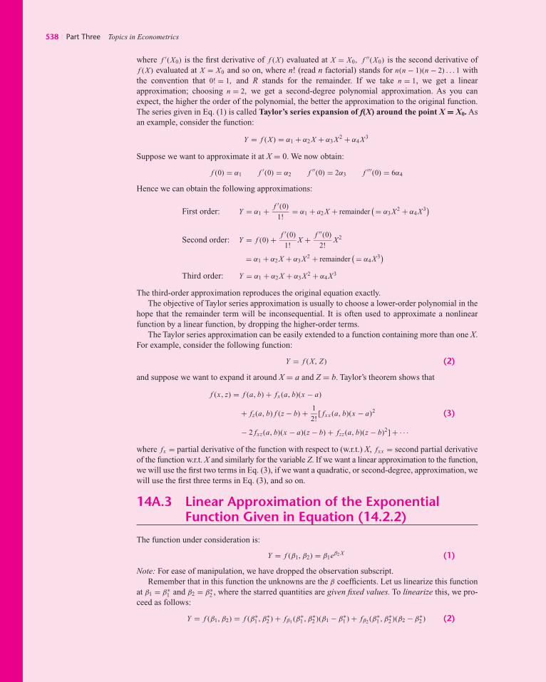
538 Part Three Topics in Econometrics
where f ′(X0) is the first derivative of f (X) evaluated at X = X0, f ′′(X0) is the second derivative off (X) evaluated at X = X0 and so on, where n! (read n factorial) stands for n(n − 1)(n − 2) . . . 1 withthe convention that 0! = 1, and R stands for the remainder. If we take n = 1, we get a linearapproximation; choosing n = 2, we get a second-degree polynomial approximation. As you canexpect, the higher the order of the polynomial, the better the approximation to the original function.The series given in Eq. (1) is called Taylor’s series expansion of f(X) around the point X = X0. Asan example, consider the function:
Y = f (X) = α1 + α2 X + α3 X2 + α4 X3
Suppose we want to approximate it at X = 0. We now obtain:
f (0) = α1 f ′(0) = α2 f ′′(0) = 2α3 f ′′′(0) = 6α4
Hence we can obtain the following approximations:
First order: Y = α1 + f ′(0)
1!= α1 + a2 X + remainder
(= α3 X2 + α4 X3)
Second order: Y = f (0) + f ′(0)
1!X + f ′′(0)
2!X2
= α1 + α2 X + α3 X2 + remainder(= α4 X3)
Third order: Y = α1 + α2 X + α3 X2 + α4 X3
The third-order approximation reproduces the original equation exactly.The objective of Taylor series approximation is usually to choose a lower-order polynomial in the
hope that the remainder term will be inconsequential. It is often used to approximate a nonlinearfunction by a linear function, by dropping the higher-order terms.
The Taylor series approximation can be easily extended to a function containing more than one X.For example, consider the following function:
Y = f (X, Z ) (2)
and suppose we want to expand it around X = a and Z = b. Taylor’s theorem shows that
f (x , z) = f (a, b) + fx (a, b)(x − a)
+ fz(a, b) f (z − b) + 1
2![ fxx (a, b)(x − a)2 (3)
− 2 fxz(a, b)(x − a)(z − b) + fzz(a, b)(z − b)2] + · · ·
where fx = partial derivative of the function with respect to (w.r.t.) X, fxx = second partial derivativeof the function w.r.t. X and similarly for the variable Z. If we want a linear approximation to the function,we will use the first two terms in Eq. (3), if we want a quadratic, or second-degree, approximation, wewill use the first three terms in Eq. (3), and so on.
14A.3 Linear Approximation of the ExponentialFunction Given in Equation (14.2.2)
The function under consideration is:
Y = f (β1, β2) = β1eβ2 X (1)
Note: For ease of manipulation, we have dropped the observation subscript. Remember that in this function the unknowns are the β coefficients. Let us linearize this function
at β1 = β∗1 and β2 = β∗
2 , where the starred quantities are given fixed values. To linearize this, we pro-ceed as follows:
Y = f (β1, β2) = f (β∗1 , β∗
2 ) + fβ1 (β∗1 , β∗
2 )(β1 − β∗1 ) + fβ2 (β∗
1 , β∗2 )(β2 − β∗
2 ) (2)
guj75772_ch14.qxd 16/08/2008 04:48 PM Page 538

Chapter 14 Nonlinear Regression Models 539
where fβ1 and fβ2 are the partial derivatives of the function (1) with respect to the unknowns and thesederivatives will be evaluated at the (assumed) starred values of the unknown parameters. Note that weare using only the first derivatives in the preceding expression, since we are linearizing the function.Now assume that β∗
1 = 0.45 and β∗2 = 0.01, which are pure guess–estimates of the true coefficients.
Now
f (β∗1 = 0.45, β∗
2 = 0.01) = 0.45e0.01Xi
(3)fβ1 = eβ2 Xi and fβ2 = β1 Xi eβ2 Xi
by the standard rules of differentiation. Evaluating these derivatives at the given values and revertingto Eq. (2), we obtain:
Yi = 0.45e0.01Xi + e0.01Xi (β1 − 0.45) + (0.45)Xi e0.01Xi (β2 − 0.01) (4)
which we write as:
(Yi − 0.45e0.01Xi ) = e0.01Xi α1 + 0.45Xi e0.01Xi α2 (5)
where
α1 = (β1 − 0.45) and α2 = (β2 − 0.01) (6)
Now let Y ∗i = (Yi − 0.45e0.01Xi ), X1 = e0.01Xi , and X2i = 0.45Xi e0.01Xi . Using these definitions and
adding the error term ui , we can finally write Eq. (5) as:
Y ∗i = α1 X1i + α2 X2i + u i (7)
Lo and behold, we now have a linear regression model. Since Y ∗i , X1i , and X2i can be readily com-
puted from the data, we can easily estimate Eq. (7) by OLS and obtain the values of α1 and α2. Then,from Eq. (6), we obtain:
β1 = α1 + 0.45 and β2 = α2 + 0.01 (8)
Call these values β∗∗1 and β∗∗
2 , respectively. Using these (revised) values, we can start the iterativeprocess given in Eq. (2), obtaining yet another set of values of the β coefficients. We can go on iter-ating (or linearizing) in this fashion until there is no substantial change in the values of the β coef-ficients. In Example 14.1, it took five iterations, but for the Mexican Cobb–Douglas example(Example 14.2), it took 32 iterations. But the underlying logic behind these iterations is the proce-dure just illustrated.
For the mutual fund fee structure example in Section 14.3, the Y*, X1, and X2 as given in Eq. (6)are as shown in Table 14.4; the basic data are given in Table 14.1. From these values, the regressionresults corresponding to Eq. (7) are:
Dependent variable: Y*
Method: Least squares
Variable Coefficient Std. Error t-Statistic Prob.
X1 0.022739 0.014126 1.609705 0.1385X2 -0.010693 0.000790 -13.52990 0.0000
R2 = 0.968324 Durbin–Watson d statistic = 0.308883
Now using Eq. (8), the reader can verify that
β∗1 = 0.4727 and β∗
2 = −0.00069 (9)
guj75772_ch14.qxd 16/08/2008 04:48 PM Page 539

540 Part Three Topics in Econometrics
Contrast these numbers with the initial guesses of 0.45 and 0.01, respectively, for the two para-meters. Using the new estimates given in Eq. (9), you can start the iterative procedure once more andgo on iterating until there is “convergence” in the sense that the final round of the estimates does notdiffer much from the round before that. Of course, you will require fewer iterations if your initialguess is closer to the final values. Also, notice that we have used only the linear term in Taylor’s seriesexpansion. If you were to use the quadratic or higher-order terms in the expansion, perhaps you wouldreach the final values much quicker. But in many applications the linear approximation has proved tobe quite good.
TABLE 14.4 Y * X1 X2
0.067744 1.005013 0.2261280.034928 1.051271 2.365360
−0.013327 1.105171 4.973269−0.062825 1.161834 7.842381−0.109831 1.221403 10.99262−0.154011 1.284025 14.44529−0.195936 1.349859 18.22309−0.236580 1.419068 22.35031−0.276921 1.491825 26.85284−0.317740 1.568312 31.75832−0.397464 1.733253 42.89801−0.446153 1.822119 49.19721
guj75772_ch14.qxd 16/08/2008 04:48 PM Page 540

541
In all the regression models that we have considered so far, we have implicitly assumed thatthe regressand, the dependent variable, or the response variable Y is quantitative, whereasthe explanatory variables are either quantitative, qualitative (or dummy), or a mixturethereof. In fact, in Chapter 9, on dummy variables, we saw how the dummy regressors areintroduced in a regression model and what role they play in specific situations.
In this chapter we consider several models in which the regressand itself is qualitative innature. Although increasingly used in various areas of social sciences and medical research,qualitative response regression models pose interesting estimation and interpretation chal-lenges. In this chapter we only touch on some of the major themes in this area, leaving thedetails to more specialized books.1
15.1 The Nature of Qualitative Response Models
Suppose we want to study the labor force participation (LFP) decision of adult males. Sincean adult is either in the labor force or not, LFP is a yes or no decision. Hence, the responsevariable, or regressand, can take only two values, say, 1 if the person is in the laborforce and 0 if he or she is not. In other words, the regressand is a binary, or dichotomous,variable. Labor economics research suggests that the LFP decision is a function of theunemployment rate, average wage rate, education, family income, etc.
As another example, consider U.S. presidential elections. Assume that there are twopolitical parties, Democratic and Republican. The dependent variable here is vote choicebetween the two political parties. Suppose we let Y = 1, if the vote is for a Democraticcandidate, and Y = 0, if the vote is for a Republican candidate. A considerable amount ofresearch on this topic has been done by the economist Ray Fair of Yale University and sev-eral political scientists.2 Some of the variables used in the vote choice are growth rate ofGDP, unemployment and inflation rates, whether the candidate is running for reelection, etc.
Chapter 15Qualitative ResponseRegression Models
1At the introductory level, the reader may find the following sources very useful. Daniel A. Powersand Yu Xie, Statistical Methods for Categorical Data Analysis, Academic Press, 2000; John H. Aldrichand Forrest Nelson, Linear Probability, Logit, and Probit Models, Sage Publications, 1984; and TimFuting Liao, Interpreting Probability Models: Logit, Probit and Other Generalized Linear Models, SagePublications, 1994. For a very comprehensive review of the literature, see G. S. Maddala, Limited-Dependent and Qualitative Variables in Econometrics, Cambridge University Press, 1983.2See, for example, Ray Fair, “Econometrics and Presidential Elections,” Journal of Economic Perspective,Summer 1996, pp. 89–102, and Michael S. Lewis-Beck, Economics and Elections: The Major WesternDemocracies, University of Michigan Press, Ann Arbor, 1980.
guj75772_ch15.qxd 19/08/2008 01:36 PM Page 541

542 Part Three Topics in Econometrics
For the present purposes, the important thing to note is that the regressand is a qualitativevariable.
One can think of several other examples where the regressand is qualitative in nature.Thus,a family either owns a house or it does not, it has disability insurance or it does not, both hus-band and wife are in the labor force or only one spouse is. Similarly, a certain drug is effectivein curing an illness or it is not. A firm decides to declare a stock dividend or not, a senatordecides to vote for a tax cut or not, a U.S. president decides to veto a bill or accept it, etc.
We do not have to restrict our response variable to yes/no or dichotomous categoriesonly. Returning to our presidential elections example, suppose there are three parties,Democratic, Republican, and Independent. The response variable here is trichotomous. Ingeneral, we can have a polychotomous (or multiple-category) response variable.
What we plan to do is to first consider the dichotomous regressand and then considervarious extensions of the basic model. But before we do that, it is important to note a fun-damental difference between a regression model where the regressand Y is quantitative anda model where it is qualitative.
In a model where Y is quantitative, our objective is to estimate its expected, or mean,value given the values of the regressors. In terms of Chapter 2, what we want isE(Yi | X1i , X2i , . . . , Xki ), where the X ’s are regressors, both quantitative and qualitative. Inmodels where Y is qualitative, our objective is to find the probability of something happen-ing, such as voting for a Democratic candidate, or owning a house, or belonging to a union,or participating in a sport, etc. Hence, qualitative response regression models are oftenknown as probability models.
In the rest of this chapter, we seek answers to the following questions:
1. How do we estimate qualitative response regression models? Can we simply estimatethem with the usual OLS procedures?
2. Are there special inference problems? In other words, is the hypothesis testing proce-dure any different from the ones we have learned so far?
3. If a regressand is qualitative, how can we measure the goodness of fit of such models?Is the conventionally computed R2 of any value in such models?
4. Once we go beyond the dichotomous regressand case, how do we estimate and interpretthe polychotomous regression models? Also, how do we handle models in which the re-gressand is ordinal, that is, an ordered categorical variable, such as schooling (less than8 years, 8 to 11 years, 12 years, and 13 or more years), or the regressand is nominal wherethere is no inherent ordering, such as ethnicity (Black, White, Hispanic, Asian, and other)?
5. How do we model phenomena such as the number of visits to one’s physician per year,the number of patents received by a firm in a given year, the number of articles publishedby a college professor in a year, the number of telephone calls received in a span of5 minutes, or the number of cars passing through a toll booth in a span of 5 minutes?Such phenomena, called count data, or rare event data, are an example of the Poisson(probability) process.
In this chapter we provide answers to some of these questions at the elementary level,for some of the topics are quite advanced and require more background in mathematics andstatistics than assumed in this book. References cited in the various footnotes may beconsulted for further details.
We start our study of qualitative response models by first considering the binaryresponse regression model. There are four approaches to developing a probability modelfor a binary response variable:
1. The linear probability model (LPM)
guj75772_ch15.qxd 19/08/2008 01:36 PM Page 542

Chapter 15 Qualitative Response Regression Models 543
2. The logit model
3. The probit model
4. The tobit model
Because of its comparative simplicity, and because it can be estimated by ordinary leastsquares (OLS), we will first consider the LPM, leaving the other two models for subsequentsections.
15.2 The Linear Probability Model (LPM)
To fix ideas, consider the following regression model:
Yi = β1 + β2 Xi + ui (15.2.1)
where X = family income and Y = 1 if the family owns a house and 0 if it does not own ahouse.
Model (15.2.1) looks like a typical linear regression model but because the regressandis binary, or dichotomous, it is called a linear probability model (LPM). This is becausethe conditional expectation of Yi given Xi , E(Yi | Xi ), can be interpreted as the conditionalprobability that the event will occur given Xi , that is, Pr (Yi = 1 | Xi ). Thus, in our exam-ple, E(Yi | Xi ) gives the probability of a family owning a house and whose income is thegiven amount Xi .
The justification of the name LPM for models like Eq. (15.2.1) can be seen as follows:Assuming E(ui ) = 0, as usual (to obtain unbiased estimators), we obtain
E(Yi | Xi ) = β1 + β2 Xi (15.2.2)
Now, if Pi = probability that Yi = 1 (that is, the event occurs), and (1 − Pi ) = probabilitythat Yi = 0 (that is, the event does not occur), the variable Yi has the following (probabil-ity) distribution:
Yi Probability
0 1 − Pi
1 Pi
Total 1
That is, Yi follows the Bernoulli probability distribution.Now, by the definition of mathematical expectation, we obtain:
E(Yi ) = 0(1 − Pi ) + 1( Pi ) = Pi (15.2.3)
Comparing Eq. (15.2.2) with Eq. (15.2.3), we can equate
E(Yi | Xi ) = β1 + β2 Xi = Pi (15.2.4)
that is, the conditional expectation of the model (15.2.1) can, in fact, be interpreted as theconditional probability of Yi . In general, the expectation of a Bernoulli random variableis the probability that the random variable equals 1. In passing note that if there are nindependent trials, each with a probability p of success and probability (1 − p) of failure,and X of these trials represent the number of successes, then X is said to follow thebinomial distribution. The mean of the binomial distribution is np and its variance isnp(1 − p). The term success is defined in the context of the problem.
guj75772_ch15.qxd 19/08/2008 01:36 PM Page 543
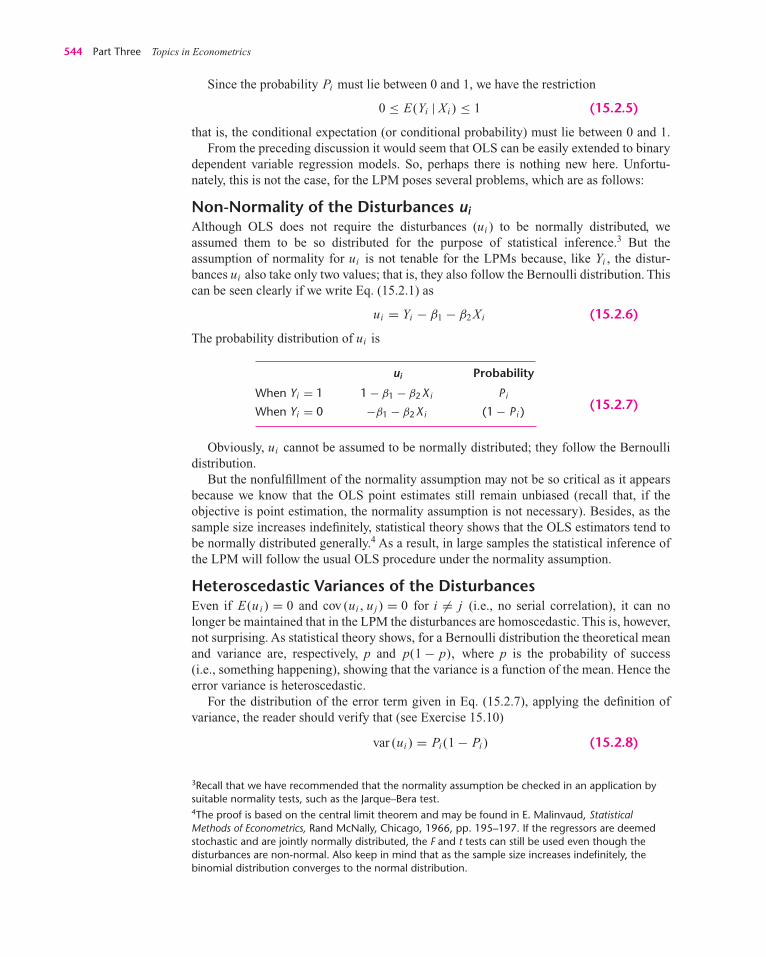
544 Part Three Topics in Econometrics
3Recall that we have recommended that the normality assumption be checked in an application bysuitable normality tests, such as the Jarque–Bera test.4The proof is based on the central limit theorem and may be found in E. Malinvaud, StatisticalMethods of Econometrics, Rand McNally, Chicago, 1966, pp. 195–197. If the regressors are deemedstochastic and are jointly normally distributed, the F and t tests can still be used even though thedisturbances are non-normal. Also keep in mind that as the sample size increases indefinitely, thebinomial distribution converges to the normal distribution.
Since the probability Pi must lie between 0 and 1, we have the restriction
0 ≤ E(Yi | Xi ) ≤ 1 (15.2.5)
that is, the conditional expectation (or conditional probability) must lie between 0 and 1.From the preceding discussion it would seem that OLS can be easily extended to binary
dependent variable regression models. So, perhaps there is nothing new here. Unfortu-nately, this is not the case, for the LPM poses several problems, which are as follows:
Non-Normality of the Disturbances uiAlthough OLS does not require the disturbances (ui ) to be normally distributed, weassumed them to be so distributed for the purpose of statistical inference.3 But theassumption of normality for ui is not tenable for the LPMs because, like Yi , the distur-bances ui also take only two values; that is, they also follow the Bernoulli distribution. Thiscan be seen clearly if we write Eq. (15.2.1) as
ui = Yi − β1 − β2 Xi (15.2.6)
The probability distribution of ui is
ui Probability
When Yi = 1 1 − β1 − β2 Xi Pi
When Yi = 0 −β1 − β2 Xi (1 − Pi )(15.2.7)
Obviously, ui cannot be assumed to be normally distributed; they follow the Bernoullidistribution.
But the nonfulfillment of the normality assumption may not be so critical as it appearsbecause we know that the OLS point estimates still remain unbiased (recall that, if theobjective is point estimation, the normality assumption is not necessary). Besides, as thesample size increases indefinitely, statistical theory shows that the OLS estimators tend tobe normally distributed generally.4 As a result, in large samples the statistical inference ofthe LPM will follow the usual OLS procedure under the normality assumption.
Heteroscedastic Variances of the DisturbancesEven if E(ui ) = 0 and cov (ui , uj ) = 0 for i �= j (i.e., no serial correlation), it can nolonger be maintained that in the LPM the disturbances are homoscedastic. This is, however,not surprising. As statistical theory shows, for a Bernoulli distribution the theoretical meanand variance are, respectively, p and p(1 − p), where p is the probability of success(i.e., something happening), showing that the variance is a function of the mean. Hence theerror variance is heteroscedastic.
For the distribution of the error term given in Eq. (15.2.7), applying the definition ofvariance, the reader should verify that (see Exercise 15.10)
var (ui ) = Pi (1 − Pi ) (15.2.8)
guj75772_ch15.qxd 19/08/2008 01:36 PM Page 544

Chapter 15 Qualitative Response Regression Models 545
5For the justification of this procedure, see Arthur S. Goldberger, Econometric Theory, John Wiley &Sons, New York, 1964, pp. 249–250. The justification is basically a large-sample one that wediscussed under the topic of feasible or estimated generalized least squares in the chapter onheteroscedasticity (see Sec. 11.6).
That is, the variance of the error term in the LPM is heteroscedastic. SincePi = E(Yi | Xi ) = β1 + β2 Xi , the variance of ui ultimately depends on the values of X andhence is not homoscedastic.
We already know that, in the presence of heteroscedasticity, the OLS estimators,although unbiased, are not efficient; that is, they do not have minimum variance. But theproblem of heteroscedasticity, like the problem of non-normality, is not insurmountable. InChapter 11 we discussed several methods of handling the heteroscedasticity problem.Since the variance of ui depends on E(Yi | Xi ), one way to resolve the heteroscedasticityproblem is to transform the model (15.2.1) by dividing it through by√
E(Yi |Xi )[1 − E(Yi |Xi )] = √Pi (1 − Pi ) = say
√wi
that is,
Yi√wi
= β1√wi
+ β2Xi√wi
+ ui√wi
(15.2.9)
As you can readily verify, the transformed error term in Eq. (15.2.9) is homoscedastic.Therefore, after estimating Eq. (15.2.1), we can now estimate Eq. (15.2.9) by OLS, whichis nothing but the weighted least squares (WLS) with wi serving as the weights.
In theory, what we have just described is fine. But in practice the true E(Yi | Xi ) isunknown; hence the weights wi are unknown. To estimate wi , we can use the following two-step procedure:5
Step 1. Run the OLS regression (15.2.1) despite the heteroscedasticity problem andobtain Yi = estimate of the true E(Yi | Xi ). Then obtain wi = Yi (1 − Yi ), the estimateof wi.
Step 2. Use the estimated wi to transform the data as shown in Eq. (15.2.9) and esti-mate the transformed equation by OLS (i.e., weighted least squares).
Although we will illustrate this procedure for our example shortly, it may be noted that wecan use White’s heteroscedasticity-corrected standard errors to deal with heteroscedastic-ity, provided the sample is reasonably large.
Even if we correct for heteroscedasticity, we first need to address another problem thatplagues LPM.
Nonfulfillment of 0 ≤ E(Yi | Xi) ≤ 1Since E(Yi | Xi ) in the linear probability models measures the conditional probability of theevent Y occurring given X, it must necessarily lie between 0 and 1. Although this is true apriori, there is no guarantee that Yi , the estimators of E(Yi | Xi ), will necessarily fulfill thisrestriction, and this is the real problem with the OLS estimation of the LPM. This happensbecause OLS does not take into account the restriction that 0 ≤ E(Yi ) ≤ 1 (an inequalityrestriction). There are two ways of finding out whether the estimated Yi lie between 0 and 1.One is to estimate the LPM by the usual OLS method and find out whether the estimated Yi
lie between 0 and 1. If some are less than 0 (that is, negative), Yi is assumed to be zero forthose cases; if they are greater than 1, they are assumed to be 1. The second procedure is todevise an estimating technique that will guarantee that the estimated conditional probabili-ties Yi will lie between 0 and 1. The logit and probit models discussed later will guaranteethat the estimated probabilities will indeed lie between the logical limits 0 and 1.
guj75772_ch15.qxd 19/08/2008 01:36 PM Page 545

546 Part Three Topics in Econometrics
Questionable Value of R2 as a Measure of Goodness of FitThe conventionally computed R2 is of limited value in the dichotomous response mod-els. To see why, consider Figure 15.1. Corresponding to a given X, Y is either 0 or 1.Therefore, all the Y values will either lie along the X axis or along the line correspond-ing to 1. Therefore, generally no LPM is expected to fit such a scatter well, whether it isthe unconstrained LPM (Figure 15.1a) or the truncated or constrained LPM (Fig-ure 15.1b), an LPM estimated in such a way that it will not fall outside the logical band0–1. As a result, the conventionally computed R2 is likely to be much lower than 1 forsuch models. In most practical applications the R2 ranges between 0.2 to 0.6. R2 in suchmodels will be high, say, in excess of 0.8 only when the actual scatter is very closelyclustered around points A and B (Figure 15.1c), for in that case it is easy to fix thestraight line by joining the two points A and B. In this case the predicted Yi will be veryclose to either 0 or 1.
Y
0X
LPM (unconstrained)
Y
0X
LPM (constrained)
0X
LPM
1
(a)
(b)
(c)
1
1B
A
Y
FIGURE 15.1Linear probabilitymodels.
guj75772_ch15.qxd 19/08/2008 01:36 PM Page 546

Chapter 15 Qualitative Response Regression Models 547
For these reasons John Aldrich and Forrest Nelson contend that “use of the coefficientof determination as a summary statistic should be avoided in models with qualitativedependent variable[s].’’6
6Aldrich and Nelson, op. cit., p. 15. For other measures of goodness of fit in models involvingdummy regressands, see T. Amemiya, “Qualitative Response Models,’’ Journal of Economic Literature,vol. 19, 1981, pp. 331–354.7One can loosely interpret the highly negative value as near improbability of owning a house whenincome is zero.
TABLE 15.1HypotheticalData on HomeOwnership (Y = 1If owns home,0 Otherwise)and Income X(Thousands ofdollars)
Family Y X Family Y X
1 0 8 21 1 222 1 16 22 1 163 1 18 23 0 124 0 11 24 0 115 0 12 25 1 166 1 19 26 0 117 1 20 27 1 208 0 13 28 1 189 0 9 29 0 11
10 0 10 30 0 1011 1 17 31 1 1712 1 18 32 0 1313 0 14 33 1 2114 1 20 34 1 2015 0 6 35 0 1116 1 19 36 0 817 1 16 37 1 1718 0 10 38 1 1619 0 8 39 0 720 1 18 40 1 17
EXAMPLE 15.1LPM:A NumericalExample
To illustrate some of the points made about the LPM in this section, we present a numer-ical example. Table 15.1 gives invented data on home ownership Y (1 = owns a house,0 = does not own a house) and family income X (thousands of dollars) for 40 families.From these data the LPM estimated by OLS was as follows:
Y i = −0.9457 + 0.1021Xi
(0.1228) (0.0082) (15.2.10)
t = (−7.6984) (12.515) R 2 = 0.8048
First, let us interpret this regression. The intercept of −0.9457 gives the “probability’’ thata family with zero income will own a house. Since this value is negative, and since proba-bility cannot be negative, we treat this value as zero, which is sensible in the present in-stance.7 The slope value of 0.1021 means that for a unit change in income (here $1,000),on the average the probability of owning a house increases by 0.1021 or about 10 percent.Of course, given a particular level of income, we can estimate the actual probability ofowning a house from Eq. (15.2.10). Thus, for X = 12 ($12,000), the estimated probabil-ity of owning a house is
(Y i | X = 12) = −0.9457 + 12(0.1021)
= 0.2795
(Continued )
guj75772_ch15.qxd 19/08/2008 01:36 PM Page 547

548 Part Three Topics in Econometrics
That is, the probability that a family with an income of $12,000 will own a house is about28 percent. Table 15.2 shows the estimated probabilities, Y i , for the various income levelslisted in the table. The most noticeable feature of this table is that six estimated values arenegative and six values are in excess of 1, demonstrating clearly the point made earlier that,although E (Yi | Xi ) is positive and less than 1, their estimators, Y i , need not be necessarilypositive or less than 1. This is one reason that the LPM is not the recommended modelwhen the dependent variable is dichotomous.
Even if the estimated Yi were all positive and less than 1, the LPM still suffers from theproblem of heteroscedasticity, which can be seen readily from Eq. (15.2.8). As a conse-quence, we cannot trust the estimated standard errors reported in Eq. (15.2.10). (Why?) Butwe can use the weighted least-squares (WLS) procedure discussed earlier to obtain moreefficient estimates of the standard errors. The necessary weights,wi , required for the applica-tion of WLS are also shown in Table 15.2. But note that since some Yi are negative and someare in excess of one, the wi corresponding to these values will be negative. Thus, we cannotuse these observations in WLS (why?), thereby reducing the number of observations, from40 to 28 in the present example.8 Omitting these observations, the WLS regression is
Y i√wi
= −1.24561√wi
+ 0.1196Xi√wi
(0.1206) (0.0069)(15.2.11)
t = (−10.332) (17.454) R 2 = 0.9214
TABLE 15.2 Actual Y, Estimated Y, and Weights wi for the Home Ownership Example
Yi Yi wi‡ √
Yi Yi wi‡ √
0 −0.129* 1 1.301†
1 0.688 0.2146 0.4633 1 0.688 0.2147 0.46331 0.893 0.0956 0.3091 0 0.280 0.2016 0.49900 0.178 0.1463 0.3825 0 0.178 0.1463 0.38250 0.280 0.2016 0.4490 1 0.688 0.2147 0.46331 0.995 0.00498 0.0705 0 0.178 0.1463 0.38251 1.098† 1 1.097†
0 0.382 0.2361 0.4859 1 0.893 0.0956 0.30910 −0.0265* 0 0.178 0.1463 0.38250 0.076 0.0702 0.2650 0 0.076 0.0702 0.26501 0.791 0.1653 0.4066 1 0.791 0.1653 0.40551 0.893 0.0956 0.3091 0 0.382 0.2361 0.48590 0.484 0.2497 0.4997 1 1.199†
1 1.097† 1 1.097†
0 −0.333* 0 0.178 0.1463 0.38251 0.995 0.00498 0.0705 0 −0.129*1 0.688 0.2147 0.4633 1 0.791 0.1653 0.40660 0.076 0.0702 0.2650 1 0.688 0.2147 0.46330 −0.129* 0 −0.231*1 0.893 0.0956 0.3091 1 0.791 0.1653 0.4066
* Treated as zero to avoid probabilities being negative.†Treated as unity to avoid probabilities exceeding one.‡Yi(1 − Yi)
EXAMPLE 15.1(Continued)
8To avoid the loss of the degrees of freedom, we could let Yi = 0.01 when the estimated Yi are nega-tive and Yi = 0.99 when they are in excess of or equal to 1. See Exercise 15.1.
wi wi
guj75772_ch15.qxd 19/08/2008 01:36 PM Page 548

Chapter 15 Qualitative Response Regression Models 549
15.3 Applications of LPM
Until the availability of readily accessible computer packages to estimate the logit and pro-bit models (to be discussed shortly), the LPM was used quite extensively because of itssimplicity. We now illustrate some of these applications.
9Malcolm S. Cohen, Samuel A. Rea, Jr., and Robert I. Lerman, A Micro Model of Labor Supply, BLS StaffPaper 4, U.S. Department of Labor, 1970.
EXAMPLE 15.2Cohen–Rea–Lerman Study9
In a study prepared for the U.S. Department of Labor, Cohen, Rea, and Lerman were in-terested in examining the labor-force participation of various categories of labor as afunction of several socioeconomic–demographic variables. In all their regressions, thedependent variable is a dummy, taking a value of 1 if a person is in the labor force, 0 ifhe or she is not. In Table 15.3 we reproduce one of their several dummy-dependent vari-able regressions.
Before interpreting the results, note these features: The preceding regression was es-timated by using the OLS. To correct for heteroscedasticity, the authors used the two-step procedure outlined previously in some of their regressions but found that thestandard errors of the estimates thus obtained did not differ materially from those ob-tained without correction for heteroscedasticity. Perhaps this result is due to the sheersize of the sample, namely, about 25,000. Because of this large sample size, the esti-mated t values may be tested for statistical significance by the usual OLS procedure eventhough the error term takes dichotomous values. The estimated R2 of 0.175 may seemrather low, but in view of the large sample size, this R2 is still significant on the basis ofthe F test (See Section 8.4). Finally, notice how the authors have blended quantitativeand qualitative variables and how they have taken into account the interaction effects.
Turning to the interpretations of the findings, we see that each slope coefficient givesthe rate of change in the conditional probability of the event occurring for a given unitchange in the value of the explanatory variable. For instance, the coefficient of −0.2753attached to the variable “age 65 and over’’ means, holding all other factors constant, theprobability of participation in the labor force by women in this age group is smaller byabout 27 percent (as compared with the base category of women aged 22 to 54). By thesame token, the coefficient of 0.3061 attached to the variable “16 or more years ofschooling’’ means, holding all other factors constant, the probability of women with thismuch education participating in the labor force is higher by about 31 percent (as com-pared with women with less than 5 years of schooling, the base category).
Now consider the interaction term marital status and age. The table shows that thelabor-force participation probability is higher by some 29 percent for those women whowere never married (as compared with the base category) and smaller by about 28 per-cent for those women who are 65 and over (again in relation to the base category). Butthe probability of participation of women who were never married and are 65 or over issmaller by about 20 percent as compared with the base category. This implies that womenaged 65 and over but never married are likely to participate in the labor force more thanthose who are aged 65 and over and are married or fall into the “other’’ category.
(Continued )
These results show that, compared with Eq. (15.2.10), the estimated standard errors aresmaller and, correspondingly, the estimated t ratios (in absolute value) are larger. But oneshould take this result with a grain of salt since in estimating Eq. (15.2.11) we had to drop12 observations. Also, since wi are estimated, the usual statistical hypothesis-testing pro-cedures are, strictly speaking, valid in the large samples (see Chapter 11).
EXAMPLE 15.1(Continued)
guj75772_ch15.qxd 19/08/2008 01:36 PM Page 549

550 Part Three Topics in Econometrics
TABLE 15.3 Labor-Force ParticipationRegression of women, age 22 and over, living in largest 96 standard metropolitan statisticalareas (SMSA) (dependent variable: in or out of labor force during 1966)
Explanatory Variable Coefficient t Ratio
Constant 0.4368 15.4
Marital statusMarried, spouse present — —Married, other 0.1523 13.8Never married 0.2915 22.0
Age 22–54 — —55–64 −0.0594 −5.765 and over −0.2753 −9.0
Years of schooling0–4 — —5–8 0.1255 5.89–11 0.1704 7.912–15 0.2231 10.616 and over 0.3061 13.3
Unemployment rate (1966), %Under 2.5 — —2.5–3.4 −0.0213 −1.63.5–4.0 −0.0269 −2.04.1–5.0 −0.0291 −2.25.1 and over −0.0311 −2.4
Employment change (1965–1966), %Under 3.5 — —3.5–6.49 0.0301 3.26.5 and over 0.0529 5.1
Relative employment opportunities, %Under 62 — —62–73.9 0.0381 3.274 and over 0.0571 3.2
FILOW, $Less than 1,500 and negative — —1,500–7,499 −0.1451 −15.47,500 and over −0.2455 −24.4
Interaction (marital status and age)Marital status Age
Other 55–64 −0.0406 −2.1Other 65 and over −0.1391 −7.4Never married 55–64 −0.1104 −3.3Never married 65 and over −0.2045 −6.4
Interaction (age and years of schooling completed)Age Years of schooling
65 and over 5–8 −0.0885 −2.865 and over 9–11 −0.0848 −2.465 and over 12–15 −0.1288 −4.065 and over 16 and over −0.1628 −3.6
R2 = 0.175No. of observations = 25,153
Note: — indicates the base or omitted category.FILOW: family income less own wage and salary income.
Source: Malcolm S. Cohen, Samuel A. Rea, Jr., and Robert I. Lerman, A Micro Model of Labor Supply, BLS Staff Paper 4,U.S. Department of Labor, 1970, Table F-6, pp. 212–213.
EXAMPLE 15.2(Continued)
guj75772_ch15.qxd 19/08/2008 01:36 PM Page 550

Chapter 15 Qualitative Response Regression Models 551
EXAMPLE 15.3Predicting aBond Rating
Based on a pooled time series and cross-sectional data of 200 Aa (high-quality) and Baa(medium-quality) bonds over the period 1961–1966, Joseph Cappelleri estimated thefollowing bond rating prediction model.10
Yi = β1 + β2 X 22i + β3 X3i + β4 X4i + β5 X5i + ui
where Yi = 1 if the bond rating is Aa (Moody’s rating)= 0 if the bond rating is Baa (Moody’s rating)
X2 = debt capitalization ratio, a measure of leverage
= dollar value of long-term debtdollar value of total capitalization
· 100
X3 = profit rate
= dollar value of after-tax incomedollar value of net total assets
· 100
X4 = standard deviation of the profit rate, a measure of profit rate variabilityX5 = net total assets (thousands of dollars), a measure of size
A priori, β2 and β4 are expected to be negative (why?) and β3 and β5 are expected to bepositive.
After correcting for heteroscedasticity and first-order autocorrelation, Cappelleri ob-tained the following results:11
Y i = 0.6860 − 0.0179X 22i + 0.0486X3i + 0.0572X4i + 0.378(E-7)X5
(0.1775) (0.0024) (0.0486) (0.0178) (0.039)(E-8) (15.3.1)
R 2 = 0.6933
Note: 0.378 (E-7) means 0.0000000378, etc.All but the coefficient of X4 have the correct signs. It is left to finance students to ra-
tionalize why the profit rate variability coefficient has a positive sign, for one would ex-pect that the greater the variability in profits, the less likely it is Moody’s would give anAa rating, other things remaining the same.
The interpretation of the regression is straightforward. For example, 0.0486 attachedto X3 means that, other things being the same, a 1 percentage point increase in theprofit rate will lead on average to about a 0.05 increase in the probability of a bond get-ting the Aa rating. Similarly, the higher the squared leveraged ratio, the lower by 0.02 isthe probability of a bond being classified as an Aa bond per unit increase in this ratio.
Following this procedure, the reader can easily interpret the rest of the coefficientsgiven in Table 15.3. From the given information, it is easy to obtain the estimates of theconditional probabilities of labor-force participation of the various categories. Thus, if wewant to find the probability for married women (other), aged 22 to 54, with 12 to 15years of schooling, with an unemployment rate of 2.5 to 3.4 percent, employmentchange of 3.5 to 6.49 percent, relative employment opportunities of 74 percent andover, and with FILOW of $7,500 and over, we obtain
0.4368 + 0.1523 + 0.2231 − 0.0213 + 0.0301 + 0.0571 − 0.2455 = 0.6326
In other words, the probability of labor-force participation by women with the preced-ing characteristics is estimated to be about 63 percent.
10Joseph Cappelleri, “Predicting a Bond Rating,’’ unpublished term paper, C.U.N.Y. The model used inthe paper is a modification of the model used by Thomas F. Pogue and Robert M. Soldofsky, “What Isin a Bond Rating?’’ Journal of Financial and Quantitative Analysis, June 1969, pp. 201–228.11Some of the estimated probabilities before correcting for heteroscedasticity were negative andsome were in excess of 1; in these cases they were assumed to be 0.01 and 0.99, respectively, tofacilitate the computation of the weights wi.
EXAMPLE 15.2(Continued)
guj75772_ch15.qxd 28/08/2008 10:01 AM Page 551

552 Part Three Topics in Econometrics
12The data used in the analysis are obtained from Douglas A. Lind, William G. Marchal, and Robert D.Mason, Statistical Techniques in Business and Economics, 11th Ed., McGraw-Hill, 2002, Appendix N,pp. 775–776. We have not used all the variables used by the authors.
EXAMPLE 15.4Who Holds aDebit Card?
Like credit cards, debit cards are now used extensively by consumers. Vendors preferthem because when you use a debit card, the amount of your purchase is automaticallydeducted from your checking or other designated account. To find out what factors de-termine the use of the debit card, we obtained data on 60 customers and considered thefollowing model:12
Yi = β1 + β2 X2i + β3 X3i + β4 X4i + ui
where Y = 1 for debit card holder, 0 otherwise; X2 = account balance in dollars; X3 =number of ATM transactions; X4 = 1 if interest is received on the account, 0 otherwise.
Since the linear probability model (LPM) exhibits heteroscedasticity, we present theusual OLS results and the OLS results corrected for heteroscedasticity in a tabular form.
Variable Coefficient Coefficient*
Constant 0.3631 0.3631(0.1796)** (0.1604)**
Balance 0.00028** 0.00028**(0.00015) (0.00014)
ATM �0.0269 �0.0269(0.208) (0.0202)
Interest �0.3019** �0.3019**(0.1448) (0.1353)
R2 0.1056 (0.1056)
Note: *denotes heteroscedasticity-corrected standard errors.
**significant at about 5% level.
As these results show, those who have higher account balances will tend to hold a debitcard. The higher the interest rate paid on account balances, the less the tendency to holda debit card. Although the ATM variable is not significant, note that it has a negativesign. This is perhaps due to ATM transaction fees.
There is not a vast difference between the estimated standard errors with and with-out heteroscedasticity correction. To save space, we have not presented the fitted values(i.e., the estimated probabilities), but they all were within the limits of 0 and 1. However,there is no guarantee that this will happen in every case.
15.4 Alternatives to LPM
As we have seen, the LPM is plagued by several problems, such as (1) non-normality of ui ,(2) heteroscedasticity of ui , (3) possibility of Yi lying outside the 0–1 range, and (4) thegenerally lower R2 values. But these problems are surmountable. For example, we canuse WLS to resolve the heteroscedasticity problem or increase the sample size to minimizethe non-normality problem. By resorting to restricted least-squares or mathematical pro-gramming techniques we can even make the estimated probabilities lie in the 0–1 interval.
But even then the fundamental problem with the LPM is that it is not logically a very at-tractive model because it assumes that Pi = E(Y = 1 | X) increases linearly with X, that is,the marginal or incremental effect of X remains constant throughout. Thus, in our homeownership example we found that as X increases by a unit ($1,000), the probability of
guj75772_ch15.qxd 19/08/2008 01:36 PM Page 552

Chapter 15 Qualitative Response Regression Models 553
owning a house increases by the same constant amount of 0.10. This is so whether the in-come level is $8,000, $10,000, $18,000, or $22,000. This seems patently unrealistic. In re-ality one would expect that Pi is nonlinearly related to Xi : At very low income a family willnot own a house but at a sufficiently high level of income, say, X*, it most likely will own ahouse. Any increase in income beyond X* will have little effect on the probability of own-ing a house. Thus, at both ends of the income distribution, the probability of owning ahouse will be virtually unaffected by a small increase in X.
Therefore, what we need is a (probability) model that has these two features: (1) As Xi
increases, Pi = E(Y = 1 | X) increases but never steps outside the 0–1 interval, and(2) the relationship between Pi and Xi is nonlinear, that is, “one which approaches zero atslower and slower rates as Xi gets small and approaches one at slower and slower rates asXi gets very large.’’13
Geometrically, the model we want would look something like Figure 15.2. Notice in thismodel that the probability lies between 0 and 1 and that it varies nonlinearly with X.
The reader will realize that the sigmoid, or S-shaped, curve in the figure very much resem-bles the cumulative distribution function (CDF) of a random variable.14 Therefore, one caneasily use the CDF to model regressions where the response variable is dichotomous, taking0–1 values. The practical question now is, which CDF? For although all CDFs are S shaped,for each random variable there is a unique CDF. For historical as well as practical reasons, theCDFs commonly chosen to represent the 0–1 response models are (1) the logistic and (2) thenormal, the former giving rise to the logit model and the latter to the probit (or normit) model.
Although a detailed discussion of the logit and probit models is beyond the scope of thisbook, we will indicate somewhat informally how one estimates such models and how oneinterprets them.
15.5 The Logit Model
We will continue with our home ownership example to explain the basic ideas underlyingthe logit model. Recall that in explaining home ownership in relation to income, the LPM was
(15.5.1)Pi = β1 + β2 Xi
13John Aldrich and Forrest Nelson, op. cit., p. 26.14As discussed in Appendix A, the CDF of a random variable X is simply the probability that it takesa value less than or equal to x0, where x0 is some specified numerical value of X. In short, F (X), theCDF of X, is F (X = x0) = P (X ≤ x0).
P
0X
–
CDF1
∞ ∞
FIGURE 15.2A cumulativedistribution function(CDF).
guj75772_ch15.qxd 19/08/2008 01:36 PM Page 553

554 Part Three Topics in Econometrics
where X is income and Pi = E(Yi = 1|Xi ) means the family owns a house. But now con-sider the following representation of home ownership:
(15.5.2)
For ease of exposition, we write Eq. (15.5.2) as
Pi = 1
1 + e−Zi= eZ
1 + eZ(15.5.3)
where Zi = β1 + β2 Xi .
Equation (15.5.3) represents what is known as the (cumulative) logistic distributionfunction.15
It is easy to verify that as Zi ranges from −∞ to +∞, Pi ranges between 0 and 1 andthat Pi is nonlinearly related to Zi (i.e., Xi ), thus satisfying the two requirements consid-ered earlier.16 But it seems that in satisfying these requirements, we have created anestimation problem because Pi is nonlinear not only in X but also in the β’s as can be seenclearly from Eq. (15.5.2). This means that we cannot use the familiar OLS procedure to es-timate the parameters.17 But this problem is more apparent than real because Eq. (15.5.2)can be linearized, which can be shown as follows.
If Pi , the probability of owning a house, is given by Eq. (15.5.3), then (1 − Pi ), theprobability of not owning a house, is
1 − Pi = 1
1 + eZi(15.5.4)
Therefore, we can write
Pi
1 − Pi= 1 + eZi
1 + e−Zi= eZi (15.5.5)
Now Pi/(1 − Pi ) is simply the odds ratio in favor of owning a house—the ratio of theprobability that a family will own a house to the probability that it will not own a house.Thus, if Pi = 0.8, it means that odds are 4 to 1 in favor of the family owning a house.
Now if we take the natural log of Eq. (15.5.5), we obtain a very interesting result,namely,
(15.5.6)Li = ln
(Pi
1 − Pi
)= Zi
= β1 + β2 Xi
Pi = 1
1 + e−(β1+β2 Xi )
15The logistic model has been used extensively in analyzing growth phenomena, such as population,GNP, money supply, etc. For theoretical and practical details of logit and probit models, see J. S. Kramer,The Logit Model for Economists, Edward Arnold Publishers, London, 1991; and G. S. Maddala, op. cit.16Note that as Zi → +∞, e−Zi tends to zero and as Zi → −∞, e−Zi increases indefinitely. Recall thate = 2.71828.17Of course, one could use nonlinear estimation techniques discussed in Chapter 14. See alsoSection 15.8.
guj75772_ch15.qxd 19/08/2008 01:36 PM Page 554

Chapter 15 Qualitative Response Regression Models 555
that is, L, the log of the odds ratio, is not only linear in X, but also (from the estimationviewpoint) linear in the parameters.18 L is called the logit, and hence the name logit modelfor models like Eq. (15.5.6).
Notice these features of the logit model.
1. As P goes from 0 to 1 (i.e., as Z varies from −∞ to +∞), the logit L goes from −∞to +∞. That is, although the probabilities (of necessity) lie between 0 and 1, the logits arenot so bounded.
2. Although L is linear in X, the probabilities themselves are not. This property is incontrast with the LPM model (15.5.1) where the probabilities increase linearly with X.19
3. Although we have included only a single X variable, or regressor, in the precedingmodel, one can add as many regressors as may be dictated by the underlying theory.
4. If L, the logit, is positive, it means that when the value of the regressor(s) increases,the odds that the regressand equals 1 (meaning some event of interest happens) increases.If L is negative, the odds that the regressand equals 1 decreases as the value of X increases.To put it differently, the logit becomes negative and increasingly large in magnitude as theodds ratio decreases from 1 to 0 and becomes increasingly large and positive as the oddsratio increases from 1 to infinity.20
5. More formally, the interpretation of the logit model given in Eq. (15.5.6) is as follows:β2, the slope, measures the change in L for a unit change in X, that is, it tells how the log-odds in favor of owning a house change as income changes by a unit, say, $1,000. Theintercept β1 is the value of the log-odds in favor of owning a house if income is zero. Likemost interpretations of intercepts, this interpretation may not have any physical meaning.
6. Given a certain level of income, say, X*, if we actually want to estimate not the oddsin favor of owning a house but the probability of owning a house itself, this can be done di-rectly from Eq. (15.5.3) once the estimates of β1 and β2 are available. This, however, raisesthe most important question: How do we estimate β1 and β2 in the first place? The answeris given in the next section.
7. Whereas the LPM assumes that Pi is linearly related to Xi, the logit model assumesthat the log of the odds ratio is linearly related to Xi .
15.6 Estimation of the Logit Model
For estimation purposes, we write Eq. (15.5.6) as follows:
Li = ln
(Pi
1 − Pi
)= β1 + β2 Xi + ui (15.6.1)
We will discuss the properties of the stochastic error term ui shortly.
18Recall that the linearity assumption of OLS does not require that the X variable be necessarily linear.So we can have X2, X3, etc., as regressors in the model. For our purpose, it is linearity in the parame-ters that is crucial.19Using calculus, it can be shown that dP /dX = β2 P (1 − P ), which shows that the rate of change inprobability with respect to X involves not only β2 but also the level of probability from which thechange is measured (but more on this in Section 15.7). In passing, note that the effect of a unitchange in Xi on P is greatest when P = 0.5 and least when P is close to 0 or 1.20This point is due to David Garson.
guj75772_ch15.qxd 19/08/2008 01:36 PM Page 555

556 Part Three Topics in Econometrics
To estimate Eq. (15.6.1), we need, apart from Xi, the values of the regressand, or logit,Li. This depends on the type of data we have for analysis. We distinguish two types of data:(1) data at the individual, or micro, level, and (2) grouped or replicated data.
Data at the Individual LevelIf we have data on individual families, as in the case of Table 15.1, OLS estimation ofEq. (15.6.1) is infeasible. This is easy to see. In terms of the data given in Table 15.1,Pi = 1 if a family owns a house and Pi = 0 if it does not own a house. But if we put thesevalues directly into the logit Li , we obtain:
Li = ln
(1
0
)if a family own a house
Li = ln
(0
1
)if a family does not own a house
Obviously, these expressions are meaningless. Therefore, if we have data at the micro, orindividual, level, we cannot estimate Eq. (15.6.1) by the standard OLS routine. In thissituation we may have to resort to the maximum-likelihood (ML) method to estimate theparameters. Although the rudiments of this method were discussed in the appendix toChapter 4, its application in the present context will be discussed in Appendix 15A, Sec-tion 15A.1, for the benefit of readers who would like to learn more about it.21 Software pack-ages, such as MICROFIT, EViews, LIMDEP, SHAZAM, PC-GIVE, STATA, and MINITAB,have built-in routines to estimate the logit model at the individual level. We will illustratethe use of the ML method later in the chapter.
Grouped or Replicated DataNow consider the data given in Table 15.4. This table gives data on several families groupedor replicated (repeat observations) according to income level and the number of familiesowning a house at each income level. Corresponding to each income level Xi , there are Ni
families, ni among whom are home owners (ni ≤ Ni ). Therefore, if we compute
Pi = ni
Ni(15.6.2)
21For a comparatively simple discussion of maximum likelihood in the context of the logit model, seeJohn Aldrich and Forrest Nelson, op. cit., pp. 49–54. See also, Alfred Demarsi, Logit Modeling: PracticalApplications, Sage Publications, Newbury Park, Calif., 1992.
TABLE 15.4Hypothetical Data onXi (Income), Ni
(Number of Familiesat Income Xi), and ni
(Number of FamiliesOwning a House)
X(thousands of dollars) Ni ni
6 40 88 50 12
10 60 1813 80 2815 100 4520 70 3625 65 3930 50 3335 40 3040 25 20
guj75772_ch15.qxd 19/08/2008 01:36 PM Page 556

Chapter 15 Qualitative Response Regression Models 557
that is, the relative frequency, we can use it as an estimate of the true Pi corresponding toeach Xi . If Ni is fairly large, Pi will be a reasonably good estimate of Pi .22 Using the esti-mated Pi, we can obtain the estimated logit as
L i = ln
(Pi
1 − Pi
)= β1 + β2 Xi (15.6.3)
which will be a fairly good estimate of the true logit Li if the number of observations Ni ateach Xi is reasonably large.
In short, given the grouped or replicated data, such as Table 15.4, one can obtain the dataon the dependent variable, the logits, to estimate the model (15.6.1). Can we then applyOLS to Eq. (15.6.3) and estimate the parameters in the usual fashion? The answer is, notquite, since we have not yet said anything about the properties of the stochastic disturbanceterm. It can be shown that if Ni is fairly large and if each observation in a given incomeclass Xi is distributed independently as a binomial variable, then
ui ∼ N
[0,
1
Ni Pi (1 − Pi )
](15.6.4)
that is, ui follows the normal distribution with zero mean and variance equal to1/[Ni Pi (1 − Pi )].23
Therefore, as in the case of the LPM, the disturbance term in the logit model is het-eroscedastic. Thus, instead of using OLS we will have to use the weighted least squares(WLS). For empirical purposes, however, we will replace the unknown Pi by Pi and use
σ 2 = 1
Ni Pi (1 − Pi )(15.6.5)
as estimator of σ 2.
We now describe the various steps in estimating the logit regression in Eq. (15.6.1):
1. For each income level X, compute the probability of owning a house as Pi = ni/Ni .
2. For each Xi , obtain the logit as24
Li = ln [Pi/(1 − Pi )]
3. To resolve the problem of heteroscedasticity, transform Eq. (15.6.1) as follows:25
√wiLi = β1
√wi + β2
√wi Xi + √
wiui (15.6.6)
22From elementary statistics recall that the probability of an event is the limit of the relative frequencyas the sample size becomes infinitely large.23As shown in elementary probability theory, Pi , the proportion of successes (here, owning a house),follows the binomial distribution with mean equal to true Pi and variance equal to Pi (1 − Pi )/Ni ; andas Ni increases indefinitely the binomial distribution approximates the normal distribution. The distri-butional properties of ui given in Eq. (15.6.4) follow from this basic theory. For details, see HenryTheil, “On the Relationships Involving Qualitative Variables,’’ American Journal of Sociology, vol. 76,July 1970, pp. 103–154.24Since Pi = ni /Ni , L i can be alternatively expressed as L i = ln ni /(Ni − ni ). In passing it shouldbe noted that to avoid Pi taking the value of 0 or 1, in practice L i is measured as L i = ln (ni + 1
2 )/(Ni − ni + 1
2 ) = ln ( Pi + 1/2Ni )/(1 − Pi + 1/2Ni ). It is recommended as a rule of thumb that Ni beat least 5 at each value of Xi . For additional details, see D. R. Cox, Analysis of Binary Data, Methuen,London, 1970, p. 33.25If we estimate Eq. (15.6.1) disregarding heteroscedasticity, the estimators, although unbiased, willnot be efficient, as we know from Chapter 11.
guj75772_ch15.qxd 19/08/2008 01:36 PM Page 557

558 Part Three Topics in Econometrics
which we write as
L∗i = β1
√wi + β2 X∗
i + vi (15.6.7)
where the weights wi = Ni Pi (1 − Pi ); L∗i = transformed or weighted Li ; X∗
i =transformed or weighted Xi ; and vi = transformed error term. It is easy to verify thatthe transformed error term vi is homoscedastic, keeping in mind that the original errorvariance is σ 2
u = 1/[Ni Pi (1 − Pi )].
4. Estimate Eq. (15.6.6) by OLS—recall that WLS is OLS on the transformed data.Notice that in Eq. (15.6.6) there is no intercept term introduced explicitly (why?).Therefore, one will have to use the regression through the origin routine to estimateEq. (15.6.6).
5. Establish confidence intervals and/or test hypotheses in the usual OLS framework, butkeep in mind that all the conclusions will be valid strictly speaking only if the sample isreasonably large (why?). Therefore, in small samples, the estimated results should beinterpreted carefully.
15.7 The Grouped Logit (Glogit) Model: A Numerical Example
To illustrate the theory just discussed, we will use the data given in Table 15.4. Since thedata in the table are grouped, the logit model based on this data will be called a groupedlogit model, glogit, for short. The necessary raw data and other relevant calculations neces-sary to implement glogit are given in Table 15.5. The results of the weighted least-squaresregression (15.6.7) based on the data given in Table 15.5 are as follows: Note that thereis no intercept in Eq. (15.6.7); hence the regression-through-the-origin procedure isappropriate here.
L∗i = −1.59474
√wi + 0.07862X∗
i
se = (0.11046) (0.00539) (15.7.1)
t = (−14.43619) (14.56675) R2 = 0.9642
The R2 is the squared correlation coefficient between actual and estimated L∗i . L∗
i and X∗i
are weighted Li and Xi , as shown in Eq. (15.6.6). Although we have shown the calculationsof the grouped logit in Table 15.5 for pedagogical reasons, this can be done easily by in-voking the glogit (grouped logit) command in STATA.
Interpretation of the Estimated Logit ModelHow do we interpret Eq. (15.7.1)? There are various ways, some intuitive and some not:
Logit InterpretationAs Eq. (15.7.1) shows, the estimated slope coefficient suggests that for a unit ($1,000) in-crease in weighted income, the weighted log of the odds in favor of owning a house goes upby 0.08 units. This mechanical interpretation, however, is not very appealing.
Odds InterpretationRemember that Li = ln [Pi/(1 − Pi )]. Therefore, taking the antilog of the estimatedlogit, we get Pi/(1 − Pi ), that is, the odds ratio. Hence, taking the antilog of Eq. (15.7.1),
guj75772_ch15.qxd 19/08/2008 01:36 PM Page 558

Chapter 15 Qualitative Response Regression Models 559
TAB
LE 1
5.5
Dat
a to
Est
imat
e th
e L
ogit
Mod
el o
f H
ome
Ow
ners
hip
Ni
n iP i
1 −
P i(2
)(3
)(4
)=
(3)÷
(2)
(5)
(6)
(7)
(8)
(9)=
(10)
=(7
)(9)
(11)
=(1
)(9)
640
80.
200.
800.
25−1
.386
36.
402.
5298
−3.5
071
15.1
788
850
120.
240.
760.
32−1
.152
69.
123.
0199
−3.4
807
24.1
592
1060
180.
300.
700.
43−0
.847
212
.60
3.54
96−3
.007
235
.496
013
8028
0.35
0.65
0.54
−0.6
190
18.2
04.
2661
−2.6
407
55.4
593
1510
045
0.45
0.55
0.82
−0.2
007
24.7
54.
9749
−0.9
985
74.6
235
2070
360.
510.
491.
040.
0570
17.4
94.
1816
0.16
7383
.650
625
6539
0.60
0.40
1.50
0.40
5415
.60
3.94
971.
6012
98.7
425
3050
330.
660.
341.
940.
6633
11.2
03.
3496
2.22
1810
0.48
8035
4030
0.75
0.25
3.0
1.09
867.
502.
7386
3.00
8695
.840
540
2520
0.80
0.20
4.0
1.38
634.
002.
000
2.77
2680
.000
0
X(t
ho
usan
ds
of
do
llars
)(1
)
P i1
−P i
Ni P
i (1
−P i
)=
wi
√w
i=
√ Ni P
i (1
−P i
)
L* i=
L i √
wi
X* i=
X i √
wi
Li=
ln(
P i)
1 −
P i√ (8
)
guj75772_ch15.qxd 19/08/2008 01:36 PM Page 559

560 Part Three Topics in Econometrics
we obtain:
Pi
1 − Pi
= e−1.59474√
wi+0.07862X∗i
(15.7.2)
= e−1.59474√
wi · e0.07862X∗i
Using a calculator, you can easily verify that e0.07862 = 1.0817. This means that for a unitincrease in weighted income, the (weighted) odds in favor of owning a house increases by1.0817 or about 8.17 percent. In general, if you take the antilog of the jth slope coefficient(in case there is more than one regressor in the model), subtract 1 from it, and multiply theresult by 100, you will get the percent change in the odds for a unit increase in the jthregressor.
Incidentally, if you want to carry the analysis in terms of unweighted logit, all youhave to do is divide the estimated L∗
i by √
wi. Table 15.6 gives the estimated weightedand unweighted logits for each observation and some other data, which we will discussshortly.
Computing ProbabilitiesSince the language of logit and odds ratio may be unfamiliar to some, we can always com-pute the probability of owning a house at a certain level of income. Suppose we want tocompute this probability at X = 20 ($20,000). Plugging this value into Eq. (15.7.1), we ob-tain: L∗
i = −0.09311 and dividing this by√
wi = 4.1816 (see Table 15.5), we obtainLi = −0.02226. Therefore, at the income level of $20,000, we have
−0.02199 = ln
(Pi
1 − Pi
)
Therefore,
P
1 − Pi
= e−0.02199 = 0.97825
Solving this for
Pi = e−0.02199
1 + e−0.02199
TABLE 15.6Lstar, Xstar,Estimated Lstar,Probability, andChange inProbability*
Probability,Lstar Xstar ELstar Logit P Change in Probability†
−3.50710 15.1788 −2.84096 −1.12299 0.24545 0.01456−3.48070 24.15920 −2.91648 −0.96575 0.27572 0.01570−3.48070 35.49600 −2.86988 −0.80850 0.30821 0.01676−2.64070 55.45930 −2.44293 −0.57263 0.36063 0.01813−0.99850 74.62350 −2.06652 −0.41538 0.39762 0.01883
0.16730 83.65060 −0.09311 −0.02226 0.49443 0.019651.60120 98.74250 1.46472 0.37984 0.59166 0.018992.22118 100.48800 2.55896 0.76396 0.68221 0.017043.00860 95.84050 3.16794 1.15677 0.76074 0.014312.77260 80.00000 3.10038 1.55019 0.82494 0.01135
*Lstar and Xstar are from Table 15.5. ELstar is the estimated Lstar. Logit is the unweighted logit. Probability is the estimatedprobability of owning a house. Change in probability is the change per unit change in income.†Computed from β2 P(1 − P ) = 0.07862P(1 − P ).
guj75772_ch15.qxd 19/08/2008 01:36 PM Page 560

Chapter 15 Qualitative Response Regression Models 561
the reader can see that the estimated probability is 0.4945. That is, given the income of$20,000, the probability of a family owning a house is about 49 percent.Table 15.6 showsthe probabilities thus computed at various income levels. As this table shows, the proba-bility of house ownership increases with income, but not linearly as with the LPM model.
Computing the Rate of Change of ProbabilityAs you can gather from Table 15.6, the probability of owning a house depends on the in-come level. How can we compute the rate of change of probabilities as income varies? Asnoted in footnote 19, that depends not only on the estimated slope coefficient β2 but also onthe level of the probability from which the change is measured; the latter of course dependson the income level at which the probability is computed.
To illustrate, suppose we want to measure the change in the probability of owning a houseat the income level $20,000. Then, from footnote 19 the change in probability for a unit in-crease in income from the level 20 (thousand) is: β(1 − P) P = 0.07862(0.5056)(0.4944) =0.01965.
It is left as an exercise for the reader to show that at income level $40,000, the change inprobability is 0.01135. Table 15.6 shows the change in probability of owning a house at var-ious income levels; these probabilities are also depicted in Figure 15.3.
To conclude our discussion of the glogit model, we present the results based on OLS, orunweighted regression, for the home ownership example:
Li = −1.6587 + 0.0792Xi
se = (0.0958) (0.0041) (15.7.3)
t = (−17.32) (19.11) r2 = 0.9786
We leave it to the reader to compare this regression with the weighted least-squares regres-sion given by Eq. (15.7.1).
15.8 The Logit Model for Ungrouped or Individual Data
To set the stage, consider the data given in Table 15.7. Letting Y = 1 if a student’s finalgrade in an intermediate microeconomics course was A and Y = 0 if the final gradewas a B or a C, Spector and Mazzeo used grade point average (GPA), TUCE, and
50.011
10 15 20 25
X, Income, thousands of dollars
30 35 40 45
0.012
0.013
0.014
0.015
Ch
ange
in
pro
bab
ilit
y
0.016
0.017
0.018
0.019
0.020FIGURE 15.3Change in probabilityin relation to income.
guj75772_ch15.qxd 19/08/2008 01:36 PM Page 561

562 Part Three Topics in Econometrics
Personalized System of Instruction (PSI) as the grade predictors. The logit model here canbe written as:
Li = ln
(Pi
1 − Pi
)= β1 + β2GPAi + β3TUCEi + β4PSIi + ui (15.8.1)
As we noted in Section 15.6, we cannot simply put Pi = 1 if a family owns a house, andzero if it does not own a house. Here neither OLS nor weighted least squares (WLS) ishelpful. We have to resort to nonlinear estimating procedures using the method of maxi-mum likelihood. The details of this method are given in Appendix 15A, Section 15A.1.Since most modern statistical packages have routines to estimate logit models on the basisof ungrouped data, we will present the results of model (15.8.1) using the data given inTable 15.7 and show how to interpret the results. The results are given in Table 15.8 in tab-ular form and are obtained by using EViews 6. Before interpreting these results, some gen-eral observations are in order.
1. Since we are using the method of maximum likelihood, which is generally a large-sample method, the estimated standard errors are asymptotic.
2. As a result, instead of using the t statistic to evaluate the statistical significance of acoefficient, we use the (standard normal) Z statistic. So inferences are based on the normaltable. Recall that if the sample size is reasonably large, the t distribution converges to thenormal distribution.
3. As noted earlier, the conventional measure of goodness of fit, R2, is not particularlymeaningful in binary regressand models. Measures similar to R2, called pseudo R2, are
TABLE 15.7 Data on the Effect of Personalized System of Instruction (PSI) on Course Grades
GPA TUCE Letter GPA TUCE LetterObservation Grade Grade PSI Grade Grade Observation Grade Grade PSI Grade Grade
1 2.66 20 0 0 C 17 2.75 25 0 0 C2 2.89 22 0 0 B 18 2.83 19 0 0 C3 3.28 24 0 0 B 19 3.12 23 1 0 B4 2.92 12 0 0 B 20 3.16 25 1 1 A5 4.00 21 0 1 A 21 2.06 22 1 0 C6 2.86 17 0 0 B 22 3.62 28 1 1 A7 2.76 17 0 0 B 23 2.89 14 1 0 C8 2.87 21 0 0 B 24 3.51 26 1 0 B9 3.03 25 0 0 C 25 3.54 24 1 1 A
10 3.92 29 0 1 A 26 2.83 27 1 1 A11 2.63 20 0 0 C 27 3.39 17 1 1 A12 3.32 23 0 0 B 28 2.67 24 1 0 B13 3.57 23 0 0 B 29 3.65 21 1 1 A14 3.26 25 0 1 A 30 4.00 23 1 1 A15 3.53 26 0 0 B 31 3.10 21 1 0 C16 2.74 19 0 0 B 32 2.39 19 1 1 A
Notes: Grade Y = 1 if the final grade is A= 0 if the final grade is B or C
TUCE = score on an examination given at the beginning of the term to test entering knowledge of macroeconomicsPSI = 1 if the new teaching method is used
= 0 otherwiseGPA = the entering grade point average
Source: L. Spector and M. Mazzeo, “Probit Analysis and Economic Education,” Journal of Economic Education, vol. 11, 1980, pp. 37–44.
guj75772_ch15.qxd 19/08/2008 01:36 PM Page 562

Chapter 15 Qualitative Response Regression Models 563
available, and there are a variety of them.26 EViews presents one such measure, the McFaddenR2, denoted by R2
McF, whose value in our example is 0.3740.27 Like R2, R2McF also ranges be-
tween 0 and 1. Another comparatively simple measure of goodness of fit is the count R2,which is defined as:
Count R2 = number of correct predictions
total number of observations(15.8.2)
Since the regressand in the logit model takes a value of 1 or zero, if the predicted prob-ability is greater than 0.5, we classify that as 1, but if it is less than 0.5, we classify thatas 0. We then count the number of correct predictions and compute the R2 as given inEq. (15.8.2). We will illustrate this shortly.
It should be noted, however, that in binary regressand models, goodness of fit is of sec-ondary importance. What matters is the expected signs of the regression coefficients andtheir statistical and/or practical significance.
4. To test the null hypothesis that all the slope coefficients are simultaneously equal tozero, the equivalent of the F test in the linear regression model is the likelihood ratio (LR)statistic. Given the null hypothesis, the LR statistic follows the χ2 distribution with dfequal to the number of explanatory variables, three in the present example. (Note: Excludethe intercept term in computing the df.)
Now let us interpret the regression results given in Eq. (15.8.1). Each slope coefficientin this equation is a partial slope coefficient and measures the change in the estimated logitfor a unit change in the value of the given regressor (holding other regressors constant).Thus, the GPA coefficient of 2.8261 means, with other variables held constant, that if GPAincreases by a unit, on average the estimated logit increases by about 2.83 units, suggestinga positive relationship between the two. As you can see, all the other regressors have a pos-itive effect on the logit, although statistically the effect of TUCE is not significant. How-ever, together all the regressors have a significant impact on the final grade, as the LRstatistic is 15.40 with a p value of about 0.0015, which is very small.
As noted previously, a more meaningful interpretation is in terms of odds, which areobtained by taking the antilog of the various slope coefficients. Thus, if you take the antilogof the PSI coefficient of 2.3786 you will get 10.7897 ( ≈ e2.3786). This suggests that
26For an accessible discussion, see J. Scott Long, Regression Models for Categorical and Limited Depen-dent Variables, Sage Publications, Newbury Park, California, 1997, pp. 102–113.27Technically, this is defined as: 1 − (LLFur/LLFr), where LLFur is the unrestricted log likelihood functionwhere all regressors are included in the model and LLFr is the restricted log likelihood function whereonly the intercept is included in the model. Conceptually, LLFur is equivalent to RSS and LLFr is equiva-lent to TSS of the linear regression model.
TABLE 15.8Regression Results ofEquation (15.8.1)
Dependent Variable: GradeMethod: ML-Binary LogitConvergence achieved after 5 iterations
Variable Coefficient Std. Error Z Statistic Probability
C -13.0213 4.931 -2.6405 0.0082GPA 2.8261 1.2629 2.2377 0.0252TUCE 0.0951 0.1415 0.67223 0.5014PSI 2.3786 1.0645 2.2345 0.0255
McFadden R2 = 0.3740 LR statistic (3 df) = 15.40419
guj75772_ch15.qxd 19/08/2008 01:36 PM Page 563

564 Part Three Topics in Econometrics
TABLE 15.9Actual and FittedValues Based onRegression inTable 15.8
Observation Actual Fitted Residual Residual Plot
1 0 0.02658 −0.026582 0 0.05950 −0.059503 0 0.18726 −0.187264 0 0.02590 −0.025905 1 0.56989 0.430116 0 0.03486 −0.034867 0 0.02650 −0.026508 0 0.05156 −0.051569 0 0.11113 −0.11113
10 1 0.69351 0.3064911 0 0.02447 −0.0244712 0 0.19000 −0.1900013 0 0.32224 −0.32224
*14 1 0.19321 0.8067915 0 0.36099 −0.3609916 0 0.03018 −0.0301817 0 0.05363 −0.0536318 0 0.03859 −0.03859
*19 0 0.58987 −0.5898720 1 0.66079 0.3392121 0 0.06138 −0.0613822 1 0.90485 0.0951523 0 0.24177 −0.24177
*24 0 0.85209 −0.8520925 1 0.83829 0.16171
*26 1 0.48113 0.5188727 1 0.63542 0.3645828 0 0.30722 −0.3072229 1 0.84170 0.1583030 1 0.94534 0.05466
*31 0 0.52912 −0.52912*32 1 0.11103 0.88897
*Incorrect predictions.
students who are exposed to the new method of teaching are more than 10 times as likelyto get an A than students who are not exposed to it, other things remaining the same.
Suppose we want to compute the actual probability of a student getting an A grade. Con-sider student number 10 in Table 15.7. Putting the actual data for this student in the esti-mated logit model given in Table 15.8, the reader can check that the estimated logit valuefor this student is 0.8178. Using Eq. (15.5.2), the reader can easily check that the estimatedprobability is 0.69351. Since this student’s actual final grade was an A, and since our logitmodel assigns a probability of 1 to a student who gets an A, the estimated probability of0.69351 is not exactly 1 but close to it.
Recall the count R2 defined earlier. Table 15.9 gives you the actual and predicted valuesof the regressand for our illustrative example. From this table you can observe that, out of32 observations, there were 6 incorrect predictions (students 14, 19, 24, 26, 31, and 32).Hence the count R2 value is 26/32 = 0.8125, whereas the McFadden R2 value is 0.3740.Although these two values are not directly comparable, they give you some idea about theorders of magnitude. Besides, one should not overplay the importance of goodness of fit inmodels where the regressand is dichotomous.
guj75772_ch15.qxd 19/08/2008 01:36 PM Page 564

Chapter 15 Qualitative Response Regression Models 565
EXAMPLE 15.5Who Owns aDebit Card?Logit Analysis
The positive sign of Balance and the negative signs of ATM and Interest are similar to theLPM, although we cannot directly compare the two. The interpretation of the coefficientsin the logit model is different from the LPM. Here, for example, if the interest rate goes upby 1 percentage point, the logit goes down by about 1.35, holding other variables con-stant. If we take the anti-log of −1.352086, we get about 0.2587. This means that if in-terest rate is paid on account balances, on average only about one-fourth of the customersare likely to hold debit cards.
From the estimated LR statistic we see that collectively the three variables are statisti-cally significant at about the 8.5 percent level. If we use the conventional 5 percentsignificance level, then these variables are only marginally significant.
The McFadden R2 value is quite low. Using the data, the reader can find out the valueof the count R2.
As noted earlier, unlike the LPM, the slope coefficients do not give us the rate of changeof probability for a unit change in the regressor. We have to calculate them as shown inTable 15.6. Fortunately, this manual task is not necessary, for statistical packages like STATAcan do this routinely. For our example, the results are as follows:
Marginal effects after logit
Y = Pr(debit) (predict)
= .42512423
Variable | dy/dx Std. Error z p > |z| [ 95% C.I. ] x
Balance | .000305 .00017 1.79 0.073 -.000029 .000639 1499.87Interest*| -.2993972 .12919 -2.32 0.020 -.552595 −.046199 .266667ATM | -.0293822 .02297 -1.28 0.201 -.074396 .015631 10.3
*dy/dx is for discrete change of dummy variable from 0 to 1.
(Continued )
We have already seen the results of the linear probability model (LPM) applied to the bankdebit card data, so let us see how the logit model does. The results are as follows:
Dependent Variable: DEBITMethod: ML–Binary Logit (Quadratic hill climbing)Sample: 1–60Included observations: 60Convergence achieved after 4 iterationsCovariance matrix computed using second derivatives
Variable Coefficient Std. Error z-Statistic Prob.
C -0.574900 0.785787 -0.731624 0.4644Balance 0.001248 0.000697 1.789897 0.0735ATM -0.120225 0.093984 -1.279205 0.2008Interest -1.352086 0.680988 -1.985478 0.0471
McFadden R-squared 0.080471 Mean dependent var. 0.433333S.D. dependent var. 0.499717 S.E. of regression 0.486274Akaike info criterion 1.391675 Sum squared resid. 13.24192Schwarz criterion 1.531298 Log likelihood -37.75024Hannan-Quinn criter. 1.446289 Restr. log likelihood -41.05391LR statistic 6.607325 Avg. log likelihood -0.629171Prob. (LR statistic) 0.085525
Obs. with Dep = 0 34 Total obs. 60Obs. with Dep = 1 26
guj75772_ch15.qxd 19/08/2008 07:01 PM Page 565

566 Part Three Topics in Econometrics
15.9 The Probit Model
As we have noted, to explain the behavior of a dichotomous dependent variable we willhave to use a suitably chosen cumulative distribution function (CDF). The logit model usesthe cumulative logistic function, as shown in Eq. (15.5.2). But this is not the only CDF thatone can use. In some applications, the normal CDF has been found useful. The estimatingmodel that emerges from the normal CDF28 is popularly known as the probit model,although sometimes it is also known as the normit model. In principle one could substitutethe normal CDF in place of the logistic CDF in Eq. (15.5.2) and proceed as in Section 16.5.Instead of following this route, we will present the probit model based on utility theory, orrational choice perspective on behavior, as developed by McFadden.29
To motivate the probit model, assume that in our home ownership example the decisionof the ith family to own a house or not depends on an unobservable utility index Ii (alsoknown as a latent variable), that is determined by one or more explanatory variables, sayincome Xi , in such a way that the larger the value of the index Ii , the greater the probabilityof a family owning a house. We express the index Ii as
Ii = β1 + β2 Xi (15.9.1)
where Xi is the income of the ith family.How is the (unobservable) index related to the actual decision to own a house? As
before, let Y = 1 if the family owns a house and Y = 0 if it does not. Now it is reasonableto assume that there is a critical or threshold level of the index, call it I ∗
i , such that if Ii
exceeds I ∗i , the family will own a house, otherwise it will not. The threshold I ∗
i , like Ii , isnot observable, but if we assume that it is normally distributed with the same mean andvariance, it is possible not only to estimate the parameters of the index given in Eq. (15.9.1)but also to get some information about the unobservable index itself. This calculation is asfollows.
Given the assumption of normality, the probability that I ∗i is less than or equal to Ii can
be computed from the standardized normal CDF as:30
Pi = P(Y = 1 | X) = P( I ∗i ≤ Ii ) = P(Zi ≤ β1 + β2 Xi ) = F(β1 + β2 Xi )
(15.9.2)
The coefficient of 0.000305 suggests that customers with higher balances have a0.03 percent higher probability of owning a debit card, but if the interest rate goes upby 1 percentage point, the probability of owning a debit card goes down by about 30 per-cent. The coefficient of ATM, although statistically insignificant, suggests that if ATMtransactions go up by a unit, the probability of owning a debit card goes down by about2.9 percent.
28See Appendix A for a discussion of the normal CDF. Briefly, if a variable X follows the normaldistribution with mean µ and variance σ2, its PDF is
f (X) = 1√2σ2π
e−(X−µ)2/2σ2
and its CDF is
F (X) =∫ X0
−∞1√
2σ2πe−(X−µ)2/2σ2
where X0 is some specified value of X.29D. McFadden, “Conditional Logit Analysis of Qualitative Choice Behavior,” in P. Zarembka (ed.),Frontiers in Econometrics, Academic Press, New York, 1973.30A normal distribution with zero mean and unit ( = 1) variance is known as a standard orstandardized normal variable (see Appendix A).
EXAMPLE 15.5(Continued)
guj75772_ch15.qxd 19/08/2008 01:36 PM Page 566

Chapter 15 Qualitative Response Regression Models 567
where P(Y = 1 | X) means the probability that an event occurs given the value(s) of the X,or explanatory, variable(s) and where Zi is the standard normal variable, i.e.,Z ∼ N (0, σ 2). F is the standard normal CDF, which written explicitly in the presentcontext is:
F( Ii ) = 1√2π
∫ Ii
−∞e−z2/2 dz
= 1√2π
∫ β1+β2 Xi
−∞e−z2/2 dz
(15.9.3)
Since P represents the probability that an event will occur, here the probability of own-ing a house, it is measured by the area of the standard normal curve from −∞ to Ii asshown in Figure 15.4a.
Now to obtain information on Ii , the utility index, as well as on β1 and β2, we take theinverse of Eq. (15.9.2) to obtain:
Ii = F−1( Ii ) = F−1( Pi )
= β1 + β2 Xi
(15.9.4)
where F−1 is the inverse of the normal CDF. What all this means can be made clear fromFigure 15.4. In panel (a) of this figure we obtain from the ordinate the (cumulative) proba-bility of owning a house given I ∗
i ≤ Ii , whereas in panel (b) we obtain from the abscissa thevalue of Ii given the value of Pi , which is simply the reverse of the former.
But how do we actually go about obtaining the index Ii as well as estimating β1 and β2?As in the case of the logit model, the answer depends on whether we have grouped data orungrouped data. We consider the two cases individually.
Probit Estimation with Grouped Data: gprobitWe will use the same data that we used for glogit, which is given in Table 15.4. Since wealready have Pi , the relative frequency (the empirical measure of probability) of owning ahouse at various income levels as shown in Table 15.5, we can use it to obtain Ii from thenormal CDF as shown in Table 15.10, or from Figure 15.5.
FIGURE 15.4Probit model: (a) givenIi, read Pi from theordinate; (b) given Pi,read Ii from theabscissa.
1
Pi
0
(a)
1
Pi
0
(b)
Pi = F(Ii) Pi = F(Ii)
Ii = β1 + β2 Xi ββ Ii = F–1(Pi)
Pr (Ii* ≤ It)
– –+ +∞ ∞ ∞ ∞
guj75772_ch15.qxd 19/08/2008 01:36 PM Page 567

568 Part Three Topics in Econometrics
Once we have the estimated Ii , estimating β1 and β2 is relatively straightforward, as weshow shortly. In passing, note that in the language of probit analysis the unobservableutility index Ii is known as the normal equivalent deviate (n.e.d.) or simply normit.Since the n.e.d. or Ii will be negative whenever Pi < 0.5, in practice the number 5 is addedto the n.e.d. and the result is called a probit.
0
1
0.66
0.4– +∞ ∞
FIGURE 15.5Normal CDF.
31The following results are not corrected for heteroscedasticity. See Exercise 15.12 for the appropriateprocedure to correct heteroscedasticity.
TABLE 15.10Estimating the IndexIi from the StandardNormal CDF
Pi li = F−1(Pi)
0.20 −0.84160.24 −0.70630.30 −0.52440.35 −0.38530.45 −0.12570.51 0.02510.60 0.25330.66 0.41250.75 0.67450.80 0.8416
Notes: (1) Pi are from Table 15.5; (2) Ii are estimated from the standard normalCDF.
EXAMPLE 15.6Illustration ofGprobit UsingHousingExample
Let us continue with our housing example. We have already presented the results of theglogit model for this example. The grouped probit (gprobit) results of the same data areas follows:
Using the n.e.d. ( = I ) given in Table 15.10, the regression results are as shown inTable 15.11.31 The regression results based on the probits ( = n.e.d. + 5) are as shownin Table 15.12.
Except for the intercept term, these results are identical with those given in theprevious table. But this should not be surprising. (Why?)
guj75772_ch15.qxd 19/08/2008 01:36 PM Page 568

Chapter 15 Qualitative Response Regression Models 569
Interpretation of the Probit Estimates in Table 15.11How do we interpret the preceding results? Suppose we want to find out the effect of a unitchange in X (income measured in thousands of dollars) on the probability that Y = 1,that is, a family purchases a house. To do this, look at Eq. (15.9.2). We want to take thederivative of this function with respect to X (that is, the rate of change of the probabilitywith respect to income). It turns out that this derivative is:
d Pi
d Xi= f (β1 + β2 Xi )β2 (15.9.5)32
where f (β1 + β2 Xi ) is the standard normal probability density function evaluated atβ1 + β2 Xi . As you will realize, this evaluation will depend on the particular value of the Xvariables. Let us take a value of X from Table 15.5, say, X = 6 (thousand dollars). Using theestimated values of the parameters given in Table 15.11, we thus want to find the normaldensity function at f [−1.0166 + 0.04846(6)] = f (−0.72548). If you refer to the normaldistribution tables, you will find that for Z = −0.72548, the normal density is about0.3066.33 Now multiplying this value by the estimated slope coefficient of 0.04846, weobtain 0.01485. This means that starting with an income level of $6,000, if the income goesup by $1,000, the probability of a family purchasing a house goes up by about 1.4 percent.(Compare this result with that given in Table 15.6.)
As you can see from the preceding discussion, compared with the LPM and logitmodels, the computation of changes in probability using the probit model is a bit tedious.
Instead of computing changes in probability, suppose you want to find the estimatedprobabilities from the fitted gprobit model. This can be done easily. Using the data in
Dependent Variable: I
Variable Coefficient Std. Error t-Statistic Probability
C -1.0166 0.0572 -17.7473 1.0397E-07Income 0.04846 0.00247 19.5585 4.8547E-08
R2 = 0.97951 Durbin–Watson statistic = 0.91384
TABLE 15.11
Dependent Variable: Probit
Variable Coefficient Std. Error t-Statistic Probability
C 3.9833 0.05728 69.5336 2.03737E-12Income 0.04846 0.00247 19.5585 4.8547E-08
R2 = 0.9795 Durbin–Watson statistic = 0.9138
Note: These results are not corrected for heteroscedasticity (see Exercise 15.12).
TABLE 15.12
EXAMPLE 15.6(Continued)
32We use the chain rule of derivatives:
dPi
dXi= dF (t)
dt· dt
dX
where t = β1 + β2 Xi .33Note that the standard normal Z can range from −∞ to +∞, but the density function f (Z) isalways positive.
guj75772_ch15.qxd 19/08/2008 01:36 PM Page 569

570 Part Three Topics in Econometrics
Table 15.11 and inserting the values of X from Table 15.5, the reader can check that theestimated n.i.d. values (to two digits) are as follows:
X 6 8 10 13 15 20 25 30 35 40Estimated n.i.d. −0.72 −0.63 −0.53 −0.39 −0.29 −0.05 0.19 0.43 0.68 0.92
Now statistical packages such as MINITAB can easily compute the (cumulative) probabil-ities associated with the various n.i.d.’s. For example, corresponding to an n.i.d. value−0.63, the estimated probability is 0.2647 and, corresponding to an n.i.d. value of 0.43, theestimated probability is 0.6691. If you compare these estimates with the actual values givenin Table 15.5, you will find that the two are fairly close, suggesting that the fitted modelis quite good. Graphically, what we have just done is already shown in Figure 15.4.
The Probit Model for Ungrouped or Individual DataLet us revisit Table 15.7, which gives data on 32 individuals about their final grade in anintermediate microeconomics course in relation to the variables GPA, TUCE, and PSI. Theresults of the logit regression are given in Table 15.8. Let us see what the probit results looklike. Notice that as in the case of the logit model for individual data, we will have to use anonlinear estimating procedure based on the method of maximum likelihood. The regres-sion results calculated by EViews 6 are given in Table 15.13.
“Qualitatively,” the results of the probit model are comparable with those obtained fromthe logit model in that GPA and PSI are individually statistically significant. Collectively,all the coefficients are statistically significant, since the value of the LR statistic is 15.5458with a p value of 0.0014. For reasons discussed in the next sections, we cannot directlycompare the logit and probit regression coefficients.
For comparative purposes, we present the results based on the linear probability model(LPM) for the grade data in Table 15.14. Again, qualitatively, the LPM results are similar
TABLE 15.13
TABLE 15.14
Dependent Variable: gradeMethod: ML—Binary probitConvergence achieved after 5 iterations
Variable Coefficient Std. Error Z-Statistic Probability
C -7.4523 2.5424 -2.9311 0.0033GPA 1.6258 0.6938 2.3430 0.0191TUCE 0.0517 0.0838 0.6166 0.5374PSI 1.4263 5950 2.3970 0.0165
LR statistic (3 df) = 15.5458 McFadden R2 = 0.3774Probability (LR stat) = 0.0014
Dependent Variable: grade
Variable Coefficient Std. Error t-Statistic Probability
C -1.4980 0.5238 -2.8594 0.0079GPA 0.4638 0.1619 2.8640 0.0078TUCE 0.0104 0.0194 0.5386 0.5943PSI 0.3785 0.1391 2.7200 0.0110
R2 = 0.4159 Durbin–Watson d = 2.3464 F-statistic = 6.6456
guj75772_ch15.qxd 19/08/2008 01:36 PM Page 570

Chapter 15 Qualitative Response Regression Models 571
to the logit and probit models in that GPA and PSI are individually statistically significantbut TUCE is not. Also, together the explanatory variables have a significant impact ongrade, as the F value of 6.6456 is statistically significant because its p value is only 0.0015.
The Marginal Effect of a Unit Change in the Value of a Regressor in the Various Regression ModelsIn the linear regression model, the slope coefficient measures the change in the averagevalue of the regressand for a unit change in the value of a regressor, with all other variablesheld constant.
In the LPM, the slope coefficient measures directly the change in the probability of anevent occurring as the result of a unit change in the value of a regressor, with the effect ofall other variables held constant.
In the logit model the slope coefficient of a variable gives the change in the log of the oddsassociated with a unit change in that variable, again holding all other variables constant. Butas noted previously, for the logit model the rate of change in the probability of an event hap-pening is given by βj Pi (1 − Pi ), where βj is the (partial regression) coefficient of the jth re-gressor. But in evaluating Pi , all the variables included in the analysis are involved.
In the probit model, as we saw earlier, the rate of change in the probability is somewhatcomplicated and is given by βj f (Zi ), where f (Zi ) is the density function of the standardnormal variable and Zi = β1 + β2 X2i + · · · + βk Xki , that is, the regression model used inthe analysis.
Thus, in both the logit and probit models all the regressors are involved in computing thechanges in probability, whereas in the LPM only the jth regressor is involved. This differencemay be one reason for the early popularity of the LPM model. Statistical packages, such asSTATA, have made the task of finding the rate of change of probability for the logit and pro-bit models much easier. So now there is no need to choose LPM just because of its simplicity.
15.10 Logit and Probit Models
Although for our grade example LPM, logit, and probit give qualitatively similar results,we will confine our attention to logit and probit models because of the problems with theLPM noted earlier. Between logit and probit, which model is preferable? In most applica-tions the models are quite similar, the main difference being that the logistic distributionhas slightly fatter tails, which can be seen from Figure 15.6. That is to say, the conditionalprobability Pi approaches 0 or 1 at a slower rate in logit than in probit. This can be seenmore clearly from Table 15.15. Therefore, there is no compelling reason to choose one overthe other. In practice many researchers choose the logit model because of its comparativemathematical simplicity.
Though the models are similar, one has to be careful in interpreting the coefficientsestimated by the two models. For example, for our grade example, the coefficient of GPAof 1.6258 of the probit model (see Table 15.13) and 2.8261 of the logit model (seeTable 15.8) are not directly comparable. The reason is that, although the standard logistic(the basis of logit) and the standard normal distributions (the basis of probit) both have amean value of zero, their variances are different; 1 for the standard normal (as we alreadyknow) and π2/3 for the logistic distribution, where π ≈ 22/7. Therefore, if you multiplythe probit coefficient by about 1.81 (which is approximately = π/
√3), you will get
approximately the logit coefficient. For our example, the probit coefficient of GPA is1.6258. Multiplying this by 1.81, we obtain 2.94, which is close to the logit coefficient.Alternatively, if you multiply a logit coefficient by 0.55 ( = 1/1.81), you will get the probit
guj75772_ch15.qxd 19/08/2008 01:36 PM Page 571

572 Part Three Topics in Econometrics
coefficient. Amemiya, however, suggests multiplying a logit estimate by 0.625 to get a bet-ter estimate of the corresponding probit estimate.34 Conversely, multiplying a probit coef-ficient by 1.6 ( = 1/0.625) gives the corresponding logit coefficient.
Incidentally, Amemiya has also shown that the coefficients of LPM and logit models arerelated as follows:
βLPM = 0.25βlogit except for intercept
and
βLPM = 0.25βlogit + 0.5 for intercept
We leave it to the reader to find out if these approximations hold for our grade example.To conclude our discussion of LPM, logit, and probit models, we consider an extended
example.
TABLE 15.15Values of CumulativeProbability Functions
Cumulative Normal Cumulative Logistic
Z
−3.0 0.0013 0.0474−2.0 0.0228 0.1192−1.5 0.0668 0.1824−1.0 0.1587 0.2689−0.5 0.3085 0.3775
0 0.5000 0.50000.5 0.6915 0.62251.0 0.8413 0.73111.5 0.9332 0.81762.0 0.9772 0.88083.0 0.9987 0.9526
0
1
P
ProbitLogit
FIGURE 15.6Logit and probitcumulativedistributions.
34T. Amemiya, “Qualitative Response Model: A Survey,” Journal of Economic Literature, vol. 19, 1981,pp. 481–536.
√12π
P1(Z) =∫
e−s2/2dsz
−∞P2(Z) = 1
1 + e−z
guj75772_ch15.qxd 19/08/2008 01:36 PM Page 572

Chapter 15 Qualitative Response Regression Models 573
35These data are from Michael P. Murray, Econometrics: A Modern Introduction, Pearson/Addison-Wesley, Boston, 2006, and can be downloaded from www.aw-bc.com/murray.
EXAMPLE 15.7To Smoke or Not to Smoke
To find out what factors determine whether or not a person becomes a smoker, we ob-tained data on 1,196 individuals.35 For each individual, there is information on education,age, income, and the price of cigarettes in 1979. The dependent variable is smoker, with1-smokers and 0-nonsmokers. Further analysis will be examined by Exercise 15.20 and thedata can be found in Table 15.28 on the textbook website. For comparative purposes,we present the results based on LPM, logit, and probit models in a tabular form (seeTable 15.16). These results have been obtained from STATA version 10.
TABLE 15.16Variables LPM Logit Probit
Constant 1.1230 2.7450 1.7019(5.96) (3.31) (3.33)
Age −0.0047 −0.0208 −0.0129(−5.70) (−5.58) (−5.66)
Education −0.0206 −0.0909 −0.0562(−4.47) (−4.40) (−4.45)
Income 1.03e–0.6 4.72e–06 2.72e–06(0.63) (0.66) (0.62)
Pcigs79 −0.0051 −0.0223 −0.0137(−1.80) (−1.79) (−1.79)
R2 0.0388 0.0297 0.0301
Notes: Figures in the parentheses are t ratios for LPM and z ratios for logit and probit. For logit andprobit, the R2 values are pseudo R2 values.
Although the coefficients of the three models are not directly comparable, qualitativelythey are similar. Thus, age, education, and price of cigarettes have a negative impact onsmoking and income has positive impact. Statistically, the income effect is zero and theprice effect is significant at about an 8 percent level. In Exercise 15.20, you are asked toapply the conversion factor to render the various coefficients comparable.
In Table 15.17 we present the marginal effect of each variable on the probability ofsmoking for each model type.
TABLE 15.17 Variables LPM Logit Probit
Age −0.0047 −0.0048 −0.0049Education −0.0206 −0.0213 −0.0213Income 1.03e–06 1.11e–06 1.03e–06Pcigs79 −0.0051 −0.0052 −0.0052
Note: Except for income, the estimated coefficients are highly statistically significant for age andeducation, and significant at about the 8 percent level for the price of cigarettes.
As you will recognize, the marginal effect of a variable on the probability of smoking forLPM is directly obtained from the estimated regression coefficients, but for the logit andprobit models they have to be computed as discussed in the chapter.
It is interesting that the marginal effects are quite similar for the three models. Forexample, if the level of education goes up, on average, the probability of someonebecoming a smoker goes down by about 2 percent.
guj75772_ch15.qxd 19/08/2008 07:01 PM Page 573

574 Part Three Topics in Econometrics
15.11 The Tobit Model
An extension of the probit model is the tobit model originally developed by James Tobin,the Nobel laureate economist. To explain this model, we continue with our home ownershipexample. In the probit model our concern was with estimating the probability of owning ahouse as a function of some socioeconomic variables. In the tobit model our interest is infinding out the amount of money a person or family spends on a house in relation tosocioeconomic variables. Now we face a dilemma: If a consumer does not purchase ahouse, obviously we have no data on housing expenditure for such consumers; we havesuch data only on consumers who actually purchase a house.
Thus consumers are divided into two groups, one consisting of, say, n1 consumers aboutwhom we have information on the regressors (say, income, mortgage interest rate, numberof people in the family, etc.) as well as the regressand (amount of expenditure on housing)and another consisting of n2 consumers about whom we have information only on theregressors but not on the regressand. A sample in which information on the regressand isavailable only for some observations is known as a censored sample.36 Therefore, the tobitmodel is also known as a censored regression model. Some authors call such modelslimited dependent variable regression models because of the restriction put on the valuestaken by the regressand.
Statistically, we can express the tobit model as
Yi = β1 + β2 Xi + ui if RHS > 0(15.11.1)= 0 otherwise
where RHS = right-hand side. Note: Additional X variables can be easily added to themodel.
Can we estimate regression (15.11.1) using only n1 observations and not worry about theremaining n2 observations? The answer is no, for the OLS estimates of the parameters ob-tained from the subset of n1 observations will be biased as well as inconsistent; that is, theyare biased even asymptotically.37
To see this, consider Figure 15.7. As the figure shows, if Y is not observed (because ofcensoring), all such observations ( = n2), denoted by crosses, will lie on the horizontal axis.If Y is observed, the observations ( = n1), denoted by dots, will lie in the X–Y plane. It isintuitively clear that if we estimate a regression line based on the n1 observations only, theresulting intercept and slope coefficients are bound to be different than if all the (n1 + n2)observations were taken into account.
How then does one estimate tobit, or censored regression, models, such as Eq. (15.11.1)?The actual mechanics involves the method of maximum likelihood, which is rather involvedand is beyond the scope of this book. But the reader can get more information about the MLmethod from the references.38
36A censored sample should be distinguished from a truncated sample in which information onthe regressors is available only if the regressand is observed. We will not pursue this topic here, butthe interested reader may consult William H. Greene, Econometric Analysis, Prentice Hall, 4th ed.,Englewood Cliffs, NJ, Chapter 19. For an intuitive discussion, see Peter Kennedy, A Guide toEconometrics, The MIT Press, Cambridge, Mass., 4th ed., 1998, Chapter 16.37The bias arises from the fact that if we consider only the n1 observations and omit the others, thereis no guarantee that E (ui ) will be necessarily zero. And without E (ui ) = 0 we cannot guarantee thatthe OLS estimates will be unbiased. This bias can be readily seen from the discussion in Appendix 3A,Eqs. (4) and (5).38See Greene, op. cit. A somewhat less technical discussion can be found in Richard Breen, RegressionModels: Censored, Sample Selected or Truncated Data, Sage Publications, Newbury Park, California, 1996.
guj75772_ch15.qxd 19/08/2008 01:36 PM Page 574

Chapter 15 Qualitative Response Regression Models 575
James Heckman has proposed an alternative to the ML method, which is comparativelysimple.39 This alternative consists of a two-step estimating procedure. In step 1, we firstestimate the probability of a consumer owning a house, which is done on the basis of theprobit model. In step 2, we estimate the model (15.11.1) by adding to it a variable (calledthe inverse Mills ratio or the hazard rate) that is derived from the probit estimate. For theactual mechanics, see the Heckman article. The Heckman procedure yields consistentestimates of the parameters of Eq. (15.11.1), but they are not as efficient as the MLestimates. Since most modern statistical software packages have the ML routine, it may bepreferable to use these packages rather than the Heckman two-step procedure.
Illustration of the Tobit Model: Ray Fair’s Model of Extramarital Affairs40
In an interesting and theoretically innovative article, Ray Fair collected a sample of 601men and women then married for the first time and analyzed their responses to a questionabout extramarital affairs.41 The variables used in this study are defined as follows:
Y = number of affairs in the past year, 0, 1, 2, 3, 4–10 (coded as 7)Z1 = 0 for female and 1 for maleZ2 = ageZ3 = number of years marriedZ4 = children: 0 if no children and 1 if childrenZ5 = religiousness on a scale of 1 to 5, 1 being antireligionZ6 = education, years: grade school = 9; high school = 12, Ph.D. or other = 20Z7 = occupation, “Hollingshead” scale, 1–7Z8 = self-rating of marriage, 1 = very unhappy, 5 = very happy
39J. J. Heckman, “Sample Selection Bias as a Specification Error,” Econometrica, vol. 47, pp. 153–161.40Ray Fair, “A Theory of Extramarital Affairs,” Journal of Political Economy, vol. 86, 1978, pp. 45–61.For the article and the data, see http://fairmodel.econ.yale.edu/rayfair/pdf/1978DAT.ZIP.41In 1969 Psychology Today published a 101-question survey on sex and asked its readers to mail intheir answers. In the July 1970 issue of the magazine the survey results were discussed on the basis ofabout 2,000 replies that were collected in electronic form. Ray Fair extracted the sample of 601 fromthese replies.
Y
X
Exp
end
itu
re o
n h
ousi
ng
: Expenditure data not available, but income data available: Both expenditure and income data available
Income× × × × × ×
×FIGURE 15.7Plot of amount ofmoney consumerspends in buying ahouse versus income.
guj75772_ch15.qxd 19/08/2008 01:36 PM Page 575

576 Part Three Topics in Econometrics
Of the 601 responses, 451 individuals had no extramarital affairs, and 150 individuals hadone or more affairs.
In terms of Figure 15.7, if we plot the number of affairs on the vertical axis and, say,education on the horizontal axis, there will be 451 observations lying along the horizontalaxis. Thus, we have a censored sample, and a tobit model may be appropriate.
Table 15.18 gives estimates of the preceding model using both (the inappropriate) OLSand (the appropriate) ML procedures. As you can see, OLS includes 451 individuals whohad no affairs and 150 who had one or more affairs. The ML method takes this into accountexplicitly but the OLS method does not, thus the difference between the two estimates.For reasons already discussed, one should rely on the ML and not the OLS estimates. Thecoefficients in the two models can be interpreted like any other regression coefficients.The negative coefficient of Z8 (marital happiness) means that the higher the marital happi-ness, the lower is the incidence of extramarital affairs, perhaps an unsurprising finding.
In passing, note that if we are interested in the probability of extramarital affairs and notin the number of such affairs, we can use the probit model assigning Y = 0 for individualswho did not have any affairs and Y = 1 for those who had such affairs, giving the resultsshown in Table 15.19. With the knowledge of probit modeling, readers should be able tointerpret the probit results given in this table on their own.
15.12 Modeling Count Data: The Poisson Regression Model
There are many phenomena where the regressand is of the count type, such as the numberof vacations taken by a family per year, the number of patents received by a firm per year,the number of visits to a dentist or a doctor per year, the number of visits to a grocery storeper week, the number of parking or speeding tickets received per year, the number of daysstayed in a hospital in a given period, the number of cars passing through a toll booth in aspan of, say, 5 minutes, and so on. The underlying variable in each case is discrete, takingonly a finite number of values. Sometimes count data can also refer to rare, or infrequent,occurrences, such as getting hit by lightning in a span of a week, winning more than one lot-tery within 2 weeks, or having two or more heart attacks in a span of 4 weeks. How do wemodel such phenomena?
TABLE 15.18OLS and TobitEstimates ofExtramarital Affairs
Explanatory Variable OLS Estimate Tobit Estimate
Intercept 5.8720 (5.1622)* 7.6084 (1.9479)†
Z1 0.0540 (0.1799) 0.9457 (0.8898)Z2 −0.0509 (−2.2536) −0.1926 (−2.3799)Z3 0.1694 (4.1109) 0.5331 (3.6368)Z4 −0.1426 (−0.4072) 1.0191 (0.7965)Z5 −0.4776 (−4.2747) −1.6990 (−4.1906)Z6 −0.0137 (−0.2143) 0.0253 (0.1113)Z7 0.1049 (1.1803) 0.2129 (0.6631)Z8 −0.7118 (−5.9319) −2.2732 (−5.4724)
R2 0.1317 0.1515
*The figures in the parentheses are the t values.†The figures in the parentheses are the Z (standard normal) values.
Note: In all there are 601 observations, of which 451 have zero values for the dependent variable (number of extramaritalaffairs) and 150 have nonzero values.
guj75772_ch15.qxd 19/08/2008 01:36 PM Page 576

Chapter 15 Qualitative Response Regression Models 577
Just as the Bernoulli distribution was chosen to model the yes/no decision in the linearprobability model, the probability distribution that is specifically suited for count data is thePoisson probability distribution. The pdf of the Poisson distribution is given by:42
f (Yi ) = µY e−µ
Y !Y = 0, 1, 2, . . . (15.12.1)
where f (Y ) denotes the probability that the variable Y takes non-negative integer values,and where Y ! (read Y factorial) stands for Y ! = Y × (Y − 1) × (Y − 2) × 2 × 1. It can beproved that
E(Y ) = µ (15.12.2)
var (Y ) = µ (15.12.3)
Notice an interesting feature of the Poisson distribution: Its variance is the same as itsmean value.
The Poisson regression model may be written as:
Yi = E(Yi ) + ui = µi + ui (15.12.4)
TABLE 15.19
Dependent Variable: YSTARMethod: ML—Binary probit
Sample: 1–601Included observations: 601Convergence achieved after 5 iterations
Variable Coefficient Std. Error Z Statistic Probability
C 0.779402 0.512549 1.520638 0.1284Z1 0.173457 0.137991 1.257015 0.2087Z2 -0.024584 0.010418 -2.359844 0.0183Z3 0.054343 0.018809 2.889278 0.0039Z4 0.216644 0.165168 1.311657 0.1896Z5 -0.185468 0.051626 -3.592551 0.0003Z6 0.011262 0.029517 0.381556 0.7028Z7 0.013669 0.041404 0.330129 0.7413Z8 -0.271791 0.053475 -5.082608 0.0000
Mean dependent var. 0.249584 S.D. dependent var. 0.433133S.E. of regression 0.410279 Akaike info criterion 1.045584Sum squared resid. 99.65088 Schwarz criterion 1.111453Log likelihood -305.1980 Hannan–Quinn criter. 1.071224Restr. log likelihood -337.6885 Avg. log likelihood -0.507817LR statistic (8 df) 64.98107 McFadden R-squared 0.096215Probability (LR stat) 4.87E-11
Obs. with Dep = 0 451 Total obs. 601Obs. with Dep = 1 150
42See any standard book on statistics for the details of this distribution.
guj75772_ch15.qxd 19/08/2008 01:36 PM Page 577

578 Part Three Topics in Econometrics
where the Y ’s are independently distributed as Poisson random variables with mean µi foreach individual expressed as
µi = E(Yi ) = β1 + β2 X2i + β3 X3i + · · · + βk Xki (15.12.5)
where the X ’s are some of the variables that might affect the mean value. For example, ifour count variable is the number of visits to the Metropolitan Museum of Art in New Yorkin a given year, this number will depend on variables such as income of the consumer,admission price, distance from the museum, and parking fees.
For estimation purposes, we write the model as:
Yi = µY e−µ
Y !+ ui (15.12.6)
with µ replaced by Eq. (5.12.5). As you can readily see, the resulting regression model willbe nonlinear in the parameters, necessitating nonlinear regression estimation discussed inthe previous chapter. Let us consider a concrete example to see how all this works out.
43John Neter, Michael H. Kutner, Christopher J. Nachtsheim, and William Wasserman, AppliedRegression Models, Irwin, 3d ed., Chicago, 1996. The data were obtained from the data disk includedin the book and refer to Exercise 14.28.
EXAMPLE 15.8An IllustrativeExample:Geriatric Studyof Frequency ofFalls
The data used here were collected by Neter et al.43 The data relate to 100 individuals65 years of age and older. The objective of the study was to record the number of falls( = Y ) suffered by these individuals in relation to gender (X2 = 0 female and 1 for male),a balance index (X3), and a strength index (X4). The higher the balance index, the morestable is the subject, and the higher the strength index, the stronger is the subject. To findout if education or education plus aerobic exercise has any effect on the number of falls,the authors introduced an additional variable (X1), called the intervention variable, suchthat X1 = 0 if only education and X1 = 1 if education plus aerobic exercise training. Thesubjects were randomly assigned to the two intervention methods.
Using EViews 6, we obtained the output in Table 15.20.
Dependent Variable: YSample: 1–100Convergence achieved after 7 iterationsY=EXP(C(0)+C(1)*X1+C(2)*X2+C(3)*X3+C(4)*X4)
Coefficient Std. Error t-Statistic Probability
C(0) 0.37020 0.3459 1.0701 0.2873C(1) -1.10036 0.1705 -6.4525 0.0000C(2) -0.02194 0.1105 -0.1985 0.8430C(3) 0.01066 0.0027 3.9483 0.0001C(4) 0.00927 0.00414 2.2380 0.0275
R2 = 0.4857 Adjusted R2 = 0.4640Log likelihood = -197.2096 Durbin–Watson statistic = 1.7358
Note: EXP( ) means e (the base of natural logarithm) raised by the expression in ( ).
TABLE 15.20
guj75772_ch15.qxd 19/08/2008 07:01 PM Page 578

Chapter 15 Qualitative Response Regression Models 579
15.13 Further Topics in Qualitative Response Regression Models
As noted at the outset, the topic of qualitative response regression models is vast. What wehave presented in this chapter are some of the basic models in this area. For those who wantto pursue this topic further, we discuss below very briefly some other models in this area.We will not pursue them here, for that would take us far away from the scope of this book.
Interpretation of Results. Keep in mind that what we have obtained in Table 15.20 isthe estimated mean value for the ith individual, µi ; that is, what we have estimated is:
µi = e0.3702−1.100366X1i −0.02194X2i +0.0106X3i +0.00927X4i (15.12.7)
To find the actual mean value for the ith subject, we need to put the values of the variousX variables for that subject. For example, subject 99 had these values: Y = 4, X1 = 0,X2 = 1, X3 = 50, and X4 = 56. Putting these values in Eq. (15.12.7), we obtain µ99 =3.3538 as the estimated mean value for the 99th subject. The actual Y value for thisindividual was 4.
Now if we want to find out the probability that a subject similar to subject 99 has lessthan 5 falls per year, we can obtain it as follows:
P (Y < 5) = P (Y = 0) + P (Y = 1) + P (Y = 2) + P (Y = 3) + P (Y = 4)
= (3.3538)0e−3.3538
0!+ (3.3538)1e−3.3538
1!+ (3.3538)2e−3.3538
2!
+ (3.3538)3e−3.3538
3!+ (3.3538)4e−3.3538
4!= 0.7491
We can also find out the marginal, or partial, effect of a regressor on the mean value ofY as follows. In terms of our illustrative example, suppose we want to find out the effect ofa unit increase in the strength index (X4) on mean Y. Since
µ = eC0+C1 X1i +C2 X2i +C 3 X3i +C4 X4i (15.12.8)
we want to find ∂µ/∂X4. Using the chain rule of calculus, it can be easily shown that thisis equal to
∂µ
∂X4= C4eC0+C1 X1i +C2 X2i +C 3 X3i +C4 X4i = C4µ (15.12.9)
That is, the rate of change of the mean value with respect to a regressor is equal to thecoefficient of that regressor times the mean value. Of course, the mean value µ willdepend on the values taken by all the regressors in the model. This is similar to the logitand probit models we discussed earlier, where the marginal contribution of a variable alsodepended on the values taken by all the variables in the model.
Returning to the statistical significance of the individual coefficients, we see that theintercept and variable X2 are individually statistically insignificant. But note that the stan-dard errors given in the table are asymptotic and hence the t values are to be interpretedasymptotically. As noted previously, generally the results of all nonlinear iterative estimat-ing procedures have validity in large samples only.
In concluding our discussion of the Poisson regression model, it may be noted that themodel makes restrictive assumptions in that the mean and the variance of the Poissonprocess are the same and that the probability of an occurrence is constant at any pointin time.
EXAMPLE 15.8(Continued)
guj75772_ch15.qxd 19/08/2008 01:36 PM Page 579

580 Part Three Topics in Econometrics
Ordinal Logit and Probit ModelsIn the bivariate logit and probit models we were interested in modeling a yes or no re-sponse variable. But often the response variable, or regressand, can have more than twooutcomes and very often these outcomes are ordinal in nature; that is, they cannot be ex-pressed on an interval scale. Frequently, in survey-type research the responses are on aLikert-type scale, such as “strongly agree,” “somewhat agree,” or “strongly disagree.” Orthe responses in an educational survey may be “less than high school,” “high school,”“college,” or “professional degrees.” Very often these responses are coded as 0 (less thanhigh school), 1 (high school), 2 (college), 3 (postgraduate). These are ordinal scales in thatthere is clear ranking among the categories but we cannot say that 2 (college education) istwice 1 (high school education) or 3 (postgraduate education) is three times 1 (high schooleducation).
To study phenomena such as the preceding, one can extend the bivariate logit and probitmodels to take into account multiple ranked categories. The arithmetic gets quite involvedas we have to use multistage normal and logistic probability distributions to allow for thevarious ranked categories. For the underlying mathematics and some of the applications,the reader may consult the Greene and Maddala texts cited earlier. At a comparativelyintuitive level, the reader may consult the Liao monograph.44 Software packages such asLIMDEP, EViews, STATA, and SHAZAM have routines to estimate ordered logit andprobit models.
Multinomial Logit and Probit ModelsIn the ordered probit and logit models the response variable has more than two ordered, orranked, categories. But there are situations where the regressand is unordered. Take, forexample, the choice of transportation mode to work. The choices may be bicycle, motor-bike, car, bus, or train. Although these are categorical responses, there is no ranking ororder here; they are essentially nominal in character. For another example, consider occu-pational classifications, such as unskilled, semiskilled, and highly skilled. Again, there is noorder here. Similarly, occupational choices such as self-employed, working for a privatefirm, working for a local government, and working for the federal government are essen-tially nominal in character.
The techniques of multinomial logit or probit models can be employed to study suchnominal categories. Again, the mathematics gets a little involved. The references cited pre-viously will give the essentials of these techniques. And the statistical packages cited earliercan be used to implement such models, if their use is required in specific cases.
Duration ModelsConsider questions such as these: (1) What determines the duration of unemploymentspells? (2) What determines the life of a light bulb? (3) What factors determine the dura-tion of a strike? (4) What determines the survival time of an HIV-positive patient?
Subjects such as these are the topic of duration models, popularly known as survivalanalysis or time-to-event data analysis. In each of the examples cited above, the keyvariable is the length of time or spell length, which is modeled as a random variable. Againthe mathematics involves the CDFs and PDFs of appropriate probability distributions.Although the technical details can be tedious, there are accessible books on this subject.45
44Tim Futing Liao, op. cit. 45See, for example, David W. Hosmer, Jr., and Stanley Lemeshow, Applied Survival Analysis, John Wiley& Sons, New York, 1999.
guj75772_ch15.qxd 19/08/2008 01:36 PM Page 580

Chapter 15 Qualitative Response Regression Models 581
Statistical packages such as STATA and LIMDEP can easily estimate such durationmodels. These packages have worked examples to aid the researcher in the use of suchmodels.
Summary andConclusions
1. Qualitative response regression models refer to models in which the response, or re-gressand, variable is not quantitative or an interval scale.
2. The simplest possible qualitative response regression model is the binary model in whichthe regressand is of the yes/no or presence/absence type.
3. The simplest possible binary regression model is the linear probability model (LPM)in which the binary response variable is regressed on the relevant explanatory vari-ables by using the standard OLS methodology. Simplicity may not be a virtue here, forthe LPM suffers from several estimation problems. Even if some of the estimationproblems can be overcome, the fundamental weakness of the LPM is that it assumesthat the probability of something happening increases linearly with the level of the re-gressor. This very restrictive assumption can be avoided if we use the logit and probitmodels.
4. In the logit model the dependent variable is the log of the odds ratio, which is a linearfunction of the regressors. The probability function that underlies the logit model is thelogistic distribution. If the data are available in grouped form, we can use OLS toestimate the parameters of the logit model, provided we take into account explicitly theheteroscedastic nature of the error term. If the data are available at the individual, ormicro, level, nonlinear-in-the-parameter estimating procedures are called for.
5. If we choose the normal distribution as the appropriate probability distribution, thenwe can use the probit model. This model is mathematically a bit difficult as it involvesintegrals. But for all practical purposes, both logit and probit models give similarresults. In practice, the choice therefore depends on the ease of computation, whichis not a serious problem with sophisticated statistical packages that are now readilyavailable.
6. If the response variable is of the count type, the model that is most frequently used in ap-plied work is the Poisson regression model, which is based on the Poisson probabilitydistribution.
7. A model that is closely related to the probit model is the tobit model, also known as acensored regression model. In this model, the response variable is observed only if acertain condition(s) is met. Thus, the question of how much one spends on a car ismeaningful only if one decides to buy a car to begin with. However, Maddala notes thatthe tobit model is “applicable only in those cases where the latent variable [i.e., thebasic variable underlying a phenomenon] can, in principle, take negative values and theobserved zero values are a consequence of censoring and nonobservability.”46
8. There are various extensions of the binary response regression models. These includeordered probit and logit and nominal probit and logit models. The philosophy underly-ing these models is the same as the simpler logit and probit models, although the math-ematics gets rather complicated.
9. Finally, we considered briefly the so-called duration models in which the durationof a phenomenon, such as unemployment or sickness, depends on several factors. In suchmodels, the length, or the spell of duration, becomes the variable of research interest.
46G. S. Maddala, Introduction to Econometrics, 2d ed., Macmillan, New York, 1992, p. 342.
guj75772_ch15.qxd 19/08/2008 01:36 PM Page 581

582 Part Three Topics in Econometrics
Questions15.1. Refer to the data given in Table 15.2. If Yi is negative, assume it to be equal to 0.01
and if it is greater than 1, assume it to be equal to 0.99. Recalculate the weights wi
and estimate the LPM using WLS. Compare your results with those given inEq. (15.2.11) and comment.
15.2. For the home ownership data given in Table 15.1, the maximum likelihoodestimates of the logit model are as follows:
L i = ln
(Pi
1 − Pi
)= −493.54 + 32.96 income
t = (−0.000008)(0.000008)
Comment on these results, bearing in mind that all values of income above 16 (thou-sand dollars) correspond to Y = 1 and all values of income below 16 correspond toY = 0. A priori, what would you expect in such a situation?
15.3. In studying the purchase of durable goods Y (Y = 1 if purchased, Y = 0 if nopurchase) as a function of several variables for a total of 762 households, Janet A.Fisher∗obtained the following LPM results:
Explanatory Variable Coefficient Standard Error
Constant 0.1411 —1957 disposable income, X1 0.0251 0.0118(Disposable income = X1)2, X2 −0.0004 0.0004Checking accounts, X3 −0.0051 0.0108Savings accounts, X4 0.0013 0.0047U.S. savings bonds, X5 −0.0079 0.0067Housing status: rent, X6 −0.0469 0.0937Housing status: own, X7 0.0136 0.0712Monthly rent, X8 −0.7540 1.0983 Monthly mortgage payments, X9 −0.9809 0.5162Personal noninstallment debt, X10 −0.0367 0.0326Age, X11 0.0046 0.0084Age squared, X12 −0.0001 0.0001Marital status, X13 (1 = married) 0.1760 0.0501Number of children, X14 0.0398 0.0358(Number of children = X14)2, X15 −0.0036 0.0072Purchase plans, X16 (1 = planned; 0 otherwise) 0.1760 0.0384
R2 = 0.1336
Notes: All financial variables are in thousands of dollars.Housing status: Rent (1 if rents; 0 otherwise).
Housing status: Own (1 if owns; 0 otherwise).
Source: Janet A. Fisher, “An Analysis of Consumer Goods Expenditure,” The Review of Economics and Statistics, vol. 64,no. 1, Table 1, 1962, p. 67.
a. Comment generally on the fit of the equation.
b. How would you interpret the coefficient of −0.0051 attached to the checking ac-counts variable? How would you rationalize the negative sign for this variable?
c. What is the rationale behind introducing the age-squared and number of children-squared variables? Why is the sign negative in both cases?
*“An Analysis of Consumer Goods Expenditure,” The Review of Economics and Statistics, vol. 64, no. 1,1962, pp. 64–71.
EXERCISES
guj75772_ch15.qxd 19/08/2008 01:36 PM Page 582

Chapter 15 Qualitative Response Regression Models 583
d. Assuming values of zero for all but the income variable, find out the conditionalprobability of a household whose income is $20,000 purchasing a durable good.
e. Estimate the conditional probability of owning durable good(s), given: X1 =$15,000, X3 = $3,000, X4 = $5,000, X6 = 0, X7 = 1, X8 = $500, X9 = $300,X10 = 0, X11 = 35, X13 = 1, X14 = 2, X16 = 0.
15.4. The R2 value in the labor-force participation regression given in Table 15.3 is 0.175,which is rather low. Can you test this value for statistical significance? Which test doyou use and why? Comment in general on the value of R2 in such models.
15.5. Estimate the probabilities of owning a house at the various income levels underly-ing the regression (15.7.1). Plot them against income and comment on the resultingrelationship.
*15.6. In the probit regression given in Table 15.11 show that the intercept is equal to−µx/σx and the slope is equal to 1/σx , where µx and σx are the mean and standarddeviation of X.
15.7. From data for 54 standard metropolitan statistical areas (SMSA), Demaris estimatedthe following logit model to explain high murder rate versus low murder rate:**
lnOi = 1.1387 + 0.0014Pi + 0.0561Ci − 0.4050Ri
se = (0.0009) (0.0227) (0.1568)
where O = the odds of a high murder rate, P = 1980 population size in thousands,C = population growth rate from 1970 to 1980, R = reading quotient, and the se arethe asymptotic standard errors.
a. How would you interpret the various coefficients?
b. Which of the coefficients are individually statistically significant?
c. What is the effect of a unit increase in the reading quotient on the odds of hav-ing a higher murder rate?
d. What is the effect of a percentage point increase in the population growth rate onthe odds of having a higher murder rate?
15.8. Compare and comment on the OLS and WLS regressions in Eqs. (15.7.3) and(15.7.1).
Empirical Exercises15.9. From the household budget survey of 1980 of the Dutch Central Bureau of Statis-
tics, J. S. Cramer obtained the following logit model based on a sample of 2,820households. (The results given here are based on the method of maximum likeli-hood and are after the third iteration.)† The purpose of the logit model was todetermine car ownership as a function of (logarithm of) income. Car ownership wasa binary variable: Y = 1 if a household owns a car, zero otherwise.
L i = −2.77231 + 0.347582 ln Income
t = (−3.35) (4.05)
χ2(1 df) = 16.681 ( p value = 0.0000)
where L i = estimated logit and where ln Income is the logarithm of income. The χ2
measures the goodness of fit of the model.
*Optional.**Demaris, op. cit., p. 46.†J. S. Cramer, An Introduction to the Logit Model for Economist, 2d ed., published and distributed byTimberlake Consultants Ltd., 2001, p. 33. These results are reproduced from the statistical packagePC-GIVE 10 published by Timberlake Consultants, p. 51.
guj75772_ch15.qxd 19/08/2008 01:36 PM Page 583

584 Part Three Topics in Econometrics
a. Interpret the estimated logit model.
b. From the estimated logit model, how would you obtain the expression for theprobability of car ownership?
c. What is the probability that a household with an income of $20,000 will own acar? And at an income level of $25,000? What is the rate of change of probabil-ity at the income level of $20,000?
d. Comment on the statistical significance of the estimated logit model.
15.10. Establish Eq. (15.2.8).
15.11. In an important study of college graduation rates of all high school matriculantsand Black-only matriculants, Bowen and Bok obtained the results in Table 15.21,based on the logit model.*
TABLE 15.21 Logistic Regression Model Predicting Graduation Rates, 1989 Entering Cohort
All Matriculants Black Only
Parameter Standard Odds Parameter Standard OddsVariable Estimate Error Ratio Estimate Error Ratio
Intercept 0.957 0.052 — 0.455 0.112 —Female 0.280 0.031 1.323 0.265 0.101 1.303Black −0.513 0.056 0.599Hispanic −0.350 0.080 0.705Asian 0.122 0.055 1.130Other race −0.330 0.104 0.719SAT > 1,299 0.331 0.059 1.393 0.128 0.248 1.137SAT 1,200–1,299 0.253 0.055 1.288 0.232 0.179 1.261SAT 1,100–1,199 0.350 0.053 1.420 0.308 0.149 1.361SAT 1,000–1,099 0.192 0.054 1.211 0.141 0.136 1.151SAT not available −0.330 0.127 0.719 0.048 0.349 1.050Top 10% of high 0.342 0.036 1.407 0.315 0.117 1.370
school classHigh school class rank −0.065 0.046 0.937 −0.065 0.148 0.937
not availableHigh socioeconomic 0.283 0.036 1.327 0.557 0.175 1.746
status (SES)Low SES −0.385 0.079 0.680 −0.305 0.143 0.737SES not available 0.110 0.050 1.116 0.031 0.172 1.031SEL-1 1.092 0.058 2.979 0.712 0.161 2.038SEL-2 0.193 0.036 1.212 0.280 0.119 1.323Women’s college −0.299 0.069 0.742 0.158 0.269 1.171Number of observations 32,524 2,354−2 log likelihood
Restricted 31,553 2,667Unrestricted 30,160 2,569
Chi square 1,393 with 18 d.f. 98 with 14 d.f.
Notes: Bold coefficients are significant at the .05 level; other coefficients are not. The omitted categories in the model are White, male, SAT < 1,000, bottom 90% of highschool class, middle SES, SEL-3, coed institution. Graduation rates are 6-year, first-school graduation rates, as defined in the notes to Appendix Table D.3.1. Institutionalselectivity categories are as defined in the notes to Appendix Table D.3.1. See Appendix B for definition of socioeconomic status (SES).
SEL-1 = institutions with mean combined SAT scores of 1,300 and above.SEL-2 = institutions with mean combined SAT scores between 1,150 and 1,299.SEL-3 = institutions with mean combined SAT scores below 1,150.
Source: Bowen and Bok, op. cit., p. 381.
*William G. Bowen and Derek Bok, The Shape of the River: Long Term Consequences of Considering Racein College and University Admissions, Princeton University Press, Princeton, NJ, 1998, p. 381.
guj75772_ch15.qxd 19/08/2008 01:36 PM Page 584

Chapter 15 Qualitative Response Regression Models 585
a. What general conclusion do you draw about graduation rates of all matriculantsand black-only matriculants?
b. The odds ratio is the ratio of two odds. Compare two groups of all matriculants,one with a SAT score of greater than 1,299 and the other with a SAT score of lessthan 1,000 (the base category). The odds ratio of 1.393 means the odds of ma-triculants in the first category graduating from college are 39 percent higher thanthose in the latter category. Do the various odds ratios shown in the table accordwith a priori expectations?
c. What can you say about the statistical significance of the estimated parameters?What about the overall significance of the estimated model?
15.12. In the probit model given in Table 15.11 the disturbance ui has this variance:
σ 2u = Pi (1 − Pi )
Ni f 2i
where fi is the standard normal density function evaluated at F−1(Pi).
a. Given the preceding variance of ui, how would you transform the model inTable 15.10 to make the resulting error term homoscedastic?
b. Use the data in Table 15.10 to show the transformed data.
c. Estimate the probit model based on the transformed data and compare the resultswith those based on the original data.
15.13. Since R2 as a measure of goodness of fit is not particularly well suited for thedichotomous dependent variable models, one suggested alternative is the χ2 testdescribed below:
χ2 =G∑
i=1
Ni ( Pi − P∗i )2
P∗i (1 − P∗
i )
where Ni = number of observations in the ith cell
Pi = actual probability of the event occurring ( = ni/Ni)
P∗I = estimated probability
G = number of cells (i.e., the number of levels at which Xi is measured, e.g.,10 in Table 15.4)
It can be shown that, for large samples, χ2 is distributed according to the χ2 distri-bution with (G − k) df, where k is the number of parameters in the estimatingmodel (k < G).
Apply the preceding χ2 test to regression (15.7.1) and comment on the resultinggoodness of fit and compare it with the reported R2 value.
15.14. Table 15.22 gives data on the results of spraying rotenone of different concentra-tions on the chrysanthemum aphis in batches of approximately fifty. Develop a suit-able model to express the probability of death as a function of the log of X, the logof dosage, and comment on the results. Also compute the χ2 test of fit discussed inExercise 15.13.
15.15. Thirteen applicants to a graduate program had quantitative and verbal scores on theGRE as listed in Table 15.23. Six students were admitted to the program.
a. Use the LPM to predict the probability of admission to the program based onquantitative and verbal scores in the GRE.
b. Is this a satisfactory model? If not, what alternative(s) do you suggest?
guj75772_ch15.qxd 19/08/2008 01:36 PM Page 585

586 Part Three Topics in Econometrics
15.16. To study the effectiveness of a price discount coupon on a six-pack of a soft drink,Douglas Montgomery and Elizabeth Peck collected the data shown in Table 15.24.A sample of 5,500 consumers was randomly assigned to the eleven discount cate-gories shown in the table, 500 per category. The response variable is whether or notconsumers redeemed the coupon within one month.
a. See if the logit model fits the data, treating the redemption rate as the dependentvariable and price discount as the explanatory variable.
b. See if the probit model does as well as the logit model.
GRE Aptitude Test Scores Admitted toGraduate Program
Student Number Quantitative, Q Verbal, V (Yes = 1, No = 0)
1 760 550 12 600 350 03 720 320 04 710 630 15 530 430 06 650 570 07 800 500 18 650 680 19 520 660 0
10 800 250 011 670 480 012 670 520 113 780 710 1
TABLE 15.23GRE Scores
Source: Donald F. Morrison,Applied Linear StatisticalMethods, Prentice-Hall, Inc.,Englewood Cliffs, NJ, 1983,p. 279 (adapted).
Concentration,Milligrams per Liter Total, Death,
X log (X ) Ni ni Pi = ni/Ni
2.6 0.4150 50 6 0.1203.8 0.5797 48 16 0.3335.1 0.7076 46 24 0.5227.7 0.8865 49 42 0.857
10.2 1.0086 50 44 0.880
TABLE 15.22Toxicity Study andRotenone onChrysanthemumAphis
Source: D. J. Fennet, ProbitAnalysis, Cambridge UniversityPress, London, 1964.
Price Discount Sample Size Number of Coupons RedeemedX, ¢ Ni ni
5 500 1007 500 1229 500 147
11 500 17613 500 21115 500 24417 500 27719 500 31021 500 34323 500 37225 500 391
TABLE 15.24Price of Soda withDiscount Coupon
Source: Douglas C.Montgomery and ElizabethA. Peck, Introduction toLinear RegressionAnalysis, John Wiley &Sons, New York, 1982,p. 243 (notation changed).
guj75772_ch15.qxd 28/08/2008 10:01 AM Page 586

Chapter 15 Qualitative Response Regression Models 587
c. What is the predicted redemption rate if the price discount was 17 cents?
d. Estimate the price discount for which 70 percent of the coupons will beredeemed.
15.17. To find out who has a bank account (checking, savings, etc.) and who doesn’t, JohnCaskey and Andrew Peterson estimated a probit model for the years 1977 and 1989,using data on U.S. households. The results are given in Table 15.25. The values ofthe slope coefficients given in the table measure the implied effect of a unit changein a regressor on the probability that a household has a bank account, thesemarginal effects being calculated at the mean values of the regressors included inthe model.
a. For 1977, what is the effect of marital status on ownership of a bank account?And for 1989? Do these results make economic sense?
b. Why is the coefficient for the minority variable negative for both 1977 and 1989?
c. How can you rationalize the negative sign for the number of children variable?
d. What does the chi-square statistic given in the table suggest? (Hint: See Exer-cise 15.13.)
TABLE 15.25 Probit Regressions Where Dependent Variable Is Ownership of a Deposit Account
1977 Data 1989 Data
Coefficients Implied Slope Coefficients Implied SlopeConstant −1.06 −2.20
(3.3)* (6.8)*Income (thousands 1991 $) 0.030 0.002 0.025 0.002
(6.9) (6.8)Married 0.127 0.008 0.235 0.023
(0.8) (1.7)Number of children −0.131 −0.009 −0.084 −0.008
(3.6) (2.0)Age of head of household (HH) 0.006 0.0004 0.021 0.002
(1.7) (6.3)Education of HH 0.121 0.008 0.128 0.012
(7.4) (7.7)Male HH −0.078 −0.005 −0.144 −0.011
(0.5) (0.9)Minority −0.750 −0.050 −0.600 −0.058
(6.8) (6.5)Employed 0.186 0.012 0.402 0.039
(1.6) (3.6)Homeowner 0.520 0.035 0.522 0.051
(4.7) (5.3)
Log likelihood −430.7 −526.0Chi-square statistic 408 602
(H0: All coefficients exceptconstant equal zero)
Number of observations 2,025 2,091Percentage in samplewith correct predictions 91 90
*Numbers in parentheses are t statistics.
Source: John P. Caskey and Andrew Peterson, “Who Has a Bank Account and Who Doesn’t: 1977 and 1989,” Research Working Paper 93-10, Federal Reserve Bank of KansasCity, October 1993.
guj75772_ch15.qxd 19/08/2008 01:36 PM Page 587

588 Part Three Topics in Econometrics
15.18. Monte Carlo study. As an aid to understanding the probit model, William Beckerand Donald Waldman assumed the following:*
E(Y | X) = −1 + 3X
Then, letting Yi = −1 + 3X + εi , where εi is assumed standard normal (i.e., zeromean and unit variance), they generated a sample of 35 observations as shown inTable 15.26.
a. From the data on Y and X given in this table, can you estimate an LPM?Remember that the true E(Y | X) = −1 + 3X .
b. Given X = 0.48, estimate E(Y | X = 0.48) and compare it with the trueE(Y | X = 0.48). Note X = 0.48.
c. Using the data on Y* and X given in Table 15.26, estimate a probit model. Youmay use any statistical package you want. The authors’ estimated probit model isthe following:
Y ∗i = −0.969 + 2.764Xi
Find out the P(Y ∗ = 1 | X = 0.48), that is, P(Y1 > 0 | X = 0.48). See if youranswer agrees with the authors’ answer of 0.64.
d. The sample standard deviation of the X values given in Table 15.26 is 0.31. Whatis the predicted change in probability if X is one standard deviation above themean value, that is, what is P(Y ∗ = 1 | X = 0.79)? The authors’ answer is 0.25.
*William E. Becker and Donald M. Waldman, “A Graphical Interpretation of Probit Coefficients,’’Journal of Economic Education, vol. 20, no. 4, Fall 1989, pp. 371–378.
Y Y* X Y Y* X
−0.3786 0 0.29 −0.3753 0 0.561.1974 1 0.59 1.9701 1 0.61
−0.4648 0 0.14 −0.4054 0 0.171.1400 1 0.81 2.4416 1 0.890.3188 1 0.35 0.8150 1 0.652.2013 1 1.00 −0.1223 0 0.232.4473 1 0.80 0.1428 1 0.260.1153 1 0.40 −0.6681 0 0.640.4110 1 0.07 1.8286 1 0.672.6950 1 0.87 −0.6459 0 0.262.2009 1 0.98 2.9784 1 0.630.6389 1 0.28 −2.3326 0 0.094.3192 1 0.99 0.8056 1 0.54
−1.9906 0 0.04 −0.8983 0 0.74−0.9021 0 0.37 −0.2355 0 0.17
0.9433 1 0.94 1.1429 1 0.57−3.2235 0 0.04 −0.2965 0 0.18
0.1690 1 0.07
TABLE 15.26Hypothetical DataSet Generated bythe Model Y = −1 +3X + ε and Y* = 1 If Y > 0
Source: William E. Becker andDonald M. Waldman, “AGraphical Interpretationof Probit Coefficients,” Journalof Economic Education, Fall1989, Table 1, p. 373.
guj75772_ch15.qxd 19/08/2008 01:36 PM Page 588

Chapter 15 Qualitative Response Regression Models 589
*Data are provided on 50 women who were diagnosed as having benign breast disease and 150 age-matched controls, with three controls per case. Trained interviewers administered a standardizedstructured questionnaire to collect information from each subject (see Pastides, et al. [1983] andPastides, et al. [1985]).†The following discussion leans heavily on John Neter, Michael H. Kutner, Christopher J. Nachsteim,and William Wasserman, Applied Linear Statistical Models, 4th ed., Irwin, 1996, pp. 573–574.
15.19. Table 15.27 on the textbook website gives data for 2,000 women regarding work(1 = a woman works, 0 = otherwise), age, marital status (1 = married, 0 = other-wise), number of children, and education (number of years of schooling). Out of atotal of 2,000 women, 657 were recorded as not being wage earners.
a. Using these data, estimate the linear probability model (LPM).
b. Using the same data, estimate a logit model and obtain the marginal effects ofthe various variables.
c. Repeat (b) for the probit model.
d. Which model would you choose? Why?
15.20. For the smokers example discussed in the text (see Section 15.10) download thedata from the textbook website in Table 15.28. See if the product of education andincome (i.e., the interaction effect) has any effect on the probability of becoming asmoker.
15.21. Download the data set Benign, which is Table 15.29, from the textbook website. Thevariable cancer is a dummy variable, where 1 = had breast cancer and 0 = did nothave breast cancer.* Using the variables age (= age of subject), HIGD (= highestgrade completed in school), CHK (= 0 if subject did not undergo regular medicalcheckups and = 1 if subject did undergo regular checkups), AGPI (= age at firstpregnancy), miscarriages (= number of miscarriages), and weight (= weight ofsubject), perform a logistic regression to conclude if these variables are statisticallyuseful for predicting whether a woman will contract breast cancer or not.
Appendix 15A
15A.1 Maximum Likelihood Estimation of the Logitand Probit Models for Individual (Ungrouped)Data†
As in the text, assume that we are interested in estimating the probability that an individual owns ahouse, given the individual’s income X. We assume that this probability can be expressed by thelogistic function (15.5.2), which is reproduced below for convenience.
Pi = 1
1 + e−(β1+β2 Xi )(1)
We do not actually observe Pi, but only observe the outcome Y = 1, if an individual owns a house,and Y = 0, if the individual does not own a house.
Since each Yi is a Bernoulli random variable, we can write
Pr (Yi = 1) = Pi (2)
Pr (Yi = 0) = (1 − Pi ) (3)
guj75772_ch15.qxd 28/08/2008 10:01 AM Page 589

590 Part Three Topics in Econometrics
Suppose we have a random sample of n observations. Letting fi (Yi ) denote the probability that Yi =1 or 0, the joint probability of observing the n Y values, i.e., f (Y1, Y2, . . . , Yn) is given as:
f (Y1, Y2, . . . , Yn) =n∏1
fi (Yi ) =n∏1
PYii (1 − Pi )
1−Yi (4)
where ∏
is the product operator. Note that we can write the joint probability density function as aproduct of individual density functions because each Yi is drawn independently and each Yi has thesame (logistic) density function. The joint probability given in Eq. (4) is known as the likelihoodfunction (LF).
Equation (4) is a little awkward to manipulate. But if we take its natural logarithm, we obtain whatis called the log likelihood function (LLF):
ln f (Y1, Y2, . . . , Yn) =n∑1
[Yi ln Pi + (1 − Yi ) ln (1 − Pi )]
=n∑1
[Yi ln Pi − Yi ln (1 − Pi ) + ln (1 − Pi )] (5)
=n∑1
[Yi ln
(Pi
1 − Pi
)]+
n∑1
ln (1 − Pi )
From Eq. (1) it is easy to verify that
(1 − Pi ) = 1
1 + eβ1+β2 Xi(6)
as well as
ln
(Pi
1 − Pi
)= β1 + β2Xi (7)
Using Eqs. (6) and (7), we can write the LLF (5) as:
ln f (Y1, Y2, . . . , Yn) =n∑1
Yi (β1 + β2 Xi ) −n∑1
ln[1 + e(β1+β2 Xi )
](8)
As you can see from Eq. (8), the log likelihood function is a function of the parameters β1 and β2,since the Xi are known.
In ML our objective is to maximize the LF (or LLF), that is, to obtain the values of the unknownparameters in such a manner that the probability of observing the given Y ’s is as high (maximum) aspossible. For this purpose, we differentiate Eq. (8) partially with respect to each unknown, set the re-sulting expressions to zero, and solve the resulting expressions. One can then apply the second-ordercondition of maximization to verify that the values of the parameters we have obtained do in factmaximize the LF.
So, you have to differentiate Eq. (8) with respect to β1 and β2 and proceed as indicated. As you willquickly realize, the resulting expressions become highly nonlinear in the parameters and no explicitsolutions can be obtained. That is why we will have to use one of the methods of nonlinear estimationdiscussed in the previous chapter to obtain numerical solutions. Once the numerical values of β1 andβ2 are obtained, we can easily estimate Eq. (1).
The ML procedure for the probit model is similar to that for the logit model, except that in Eq. (1)we use the normal CDF rather than the logistic CDF. The resulting expression becomes rather com-plicated, but the general idea is the same. So, we will not pursue it any further.
guj75772_ch15.qxd 19/08/2008 01:36 PM Page 590

591
In Chapter 1 we discussed briefly the types of data that are generally available for empir-ical analysis, namely, time series, cross section, and panel. In time series data we observethe values of one or more variables over a period of time (e.g., GDP for several quartersor years). In cross-section data, values of one or more variables are collected for severalsample units, or subjects, at the same point in time (e.g., crime rates for 50 states in theUnited States for a given year). In panel data the same cross-sectional unit (say a familyor a firm or a state) is surveyed over time. In short, panel data have space as well as timedimensions.
We have already seen an example of this in Table 1.1, which gives data on eggs producedand their prices for 50 states in the United States for years 1990 and 1991. For any givenyear, the data on eggs and their prices represent a cross-sectional sample. For any givenstate, there are two time series observations on eggs and their prices. Thus, we have in all100 (pooled) observations on eggs produced and their prices.
Another example of panel data was given in Table 1.2, which gives data on investment,value of the firm, and capital stock for four companies for the period 1935–1954. The datafor each company over the period 1935–1954 constitute time series data, with 20 observa-tions; data, for all four companies for a given year is an example of cross-section data, withonly four observations; and data for all the companies for all the years is an example ofpanel data, with a total of 80 observations.
There are other names for panel data, such as pooled data (pooling of time seriesand cross-sectional observations), combination of time series and cross-section data,micropanel data, longitudinal data (a study over time of a variable or group of subjects),event history analysis (studying the movement over time of subjects through successivestates or conditions), and cohort analysis (e.g., following the career path of 1965 graduatesof a business school). Although there are subtle variations, all these names essentially con-note movement over time of cross-sectional units. We will therefore use the term panel datain a generic sense to include one or more of these terms. And we will call regression mod-els based on such data panel data regression models.
Panel data are now being used increasingly in economic research. Some of the well-known panel data sets are:
1. The Panel Study of Income Dynamics (PSID) conducted by the Institute of SocialResearch at the University of Michigan. Started in 1968, each year the Institute col-lects data on some 5,000 families about various socioeconomic and demographicvariables.
Chapter 16Panel Data RegressionModels
guj75772_ch16.qxd 22/08/2008 07:13 PM Page 591

592 Part Three Topics in Econometrics
2. The Bureau of the Census of the Department of Commerce conducts a survey similar toPSID, called the Survey of Income and Program Participation (SIPP). Four times ayear respondents are interviewed about their economic condition.
3. The German Socio-Economic Panel (GESOEP) studied 1,761 individuals every yearbetween 1984 and 2002. Information on year of birth, gender, life satisfaction, maritalstatus, individual labor earnings, and annual hours of work was collected for each indi-vidual for the period 1984 to 2002.
There are also many other surveys that are conducted by various governmental agencies,such as:
Household, Income and Labor Dynamics in Australia Survey (HILDA)
British Household Panel Survey (BHPS)
Korean Labor and Income Panel Study (KLIPS)
At the outset a warning is in order: The topic of panel data regressions is vast, and some ofthe mathematics and statistics involved are quite complicated. We only hope to touch on someof the essentials of the panel data regression models, leaving the details for the references.1 Butbe forewarned that some of these references are highly technical. Fortunately, user-friendlysoftware packages such as LIMDEP, PC-GIVE, SAS, STATA, SHAZAM, and EViews, amongothers, have made the task of actually implementing panel data regressions quite easy.
16.1 Why Panel Data?
What are the advantages of panel data over cross-section or time series data? Baltagi liststhe following advantages of panel data:2
1. Since panel data relate to individuals, firms, states, countries, etc., over time, there isbound to be heterogeneity in these units. The techniques of panel data estimation cantake such heterogeneity explicitly into account by allowing for subject-specific vari-ables, as we shall show shortly. We use the term subject in a generic sense to includemicrounits such as individuals, firms, states, and countries.
2. By combining time series of cross-section observations, panel data gives “more infor-mative data, more variability, less collinearity among variables, more degrees of free-dom and more efficiency.”
3. By studying the repeated cross section of observations, panel data are better suited tostudy the dynamics of change. Spells of unemployment, job turnover, and labor mobilityare better studied with panel data.
4. Panel data can better detect and measure effects that simply cannot be observed in purecross-section or pure time series data. For example, the effects of minimum wage laws
1Some of the references are G. Chamberlain, “Panel Data,” in Handbook of Econometrics, vol. II; Z. Griliches and M. D. Intriligator, eds., North-Holland Publishers, 1984, Chapter 22; C. Hsiao,Analysis of Panel Data, Cambridge University Press, 1986; G. G. Judge, R. C. Hill, W. E. Griffiths, H. Lutkepohl, and T. C. Lee, Introduction to the Theory and Practice of Econometrics, 2d ed., John Wiley& Sons, New York, 1985, Chapter 11; W. H. Greene, Econometric Analysis, 6th ed., Prentice-Hall, Englewood Cliffs, NJ, 2008, Chapter 9; Badi H. Baltagi, Econometric Analysis of Panel Data, John Wileyand Sons, New York, 1995; and J. M. Wooldridge, Econometric Analysis of Cross Section and PanelData, MIT Press, Cambridge, Mass., 1999. For a detailed treatment of the subject with empirical applications, see Edward W. Frees, Longitudinal and Panel Data: Analysis and Applications in the SocialSciences, Cambridge University Press, New York, 2004.2Baltagi, op. cit., pp. 3–6.
guj75772_ch16.qxd 22/08/2008 07:13 PM Page 592

Chapter 16 Panel Data Regression Models 593
on employment and earnings can be better studied if we include successive waves ofminimum wage increases in the federal and/or state minimum wages.
5. Panel data enables us to study more complicated behavioral models. For example,phenomena such as economies of scale and technological change can be better handledby panel data than by pure cross-section or pure time series data.
6. By making data available for several thousand units, panel data can minimize the biasthat might result if we aggregate individuals or firms into broad aggregates.
In short, panel data can enrich empirical analysis in ways that may not be possible if we use onlycross-section or time series data. This is not to suggest that there are no problems with paneldata modeling. We will discuss them after we cover some theory and discuss some examples.
16.2 Panel Data: An Illustrative Example
To set the stage, let us consider a concrete example. Consider the data given as Table 16.1on the textbook website, which were originally collected by Professor Moshe Kim and arereproduced from William Greene.3 The data analyzes the costs of six airline firms for theperiod 1970–1984, for a total of 90 panel data observations.
The variables are defined as: I = airline id; T = year id; Q = output, in revenue passen-ger miles, an index number; C = total cost, in $1,000; PF = fuel price; and LF = load fac-tor, the average capacity utilization of the fleet.
Suppose we are interested in finding out how total cost (C) behaves in relation to output (Q),fuel price (PF), and load factor (LF). In short, we wish to estimate an airline cost function.
How do we go about estimating this function? Of course, we can estimate the cost func-tion for each airline using the data for 1970–1984 (i.e., a time series regression). This canbe accomplished with the usual ordinary least squares (OLS) procedure. We will have in allsix cost functions, one for each airline. But then we neglect the information about the otherairlines which operate in the same (regulatory) environment.
We can also estimate a cross-section cost function (i.e., a cross-section regression).We will have in all 15 cross-section regressions, one for each year. But this would not makemuch sense in the present context, for we have only six observations per year and there arethree explanatory variables (plus the intercept term); we will have very few degrees of free-dom to do a meaningful analysis. Also, we will not “exploit” the panel nature of our data.
Incidentally, the panel data in our example is called a balanced panel; a panel is said tobe balanced if each subject (firm, individuals, etc.) has the same number of observations. Ifeach entity has a different number of observations, then we have an unbalanced panel. Formost of this chapter, we will deal with balanced panels. In the panel data literature you willalso come across the terms short panel and long panel. In a short panel the number ofcross-sectional subjects, N, is greater than the number of time periods, T. In a long panel, itis T that is greater than N. As we discuss later, the estimating techniques can depend onwhether we have a short panel or a long one.
What, then, are the options? There are four possibilities:
1. Pooled OLS model. We simply pool all 90 observations and estimate a “grand”regression, neglecting the cross-section and time series nature of our data.
2. The fixed effects least squares dummy variable (LSDV) model. Here we pool all 90observations, but allow each cross-section unit (i.e., airline in our example) to have itsown (intercept) dummy variable.
3William H. Greene, Econometric Analysis, 6th ed., 2008. Data are located at http://pages.stern.nyu.edu/~wgreen/Text/econometricanalysis.htm.
guj75772_ch16.qxd 22/08/2008 07:13 PM Page 593

594 Part Three Topics in Econometrics
3. The fixed effects within-group model. Here also we pool all 90 observations, but foreach airline we express each variable as a deviation from its mean value and then esti-mate an OLS regression on such mean-corrected or “de-meaned” values.
4. The random effects model (REM). Unlike the LSDV model, in which we allow eachairline to have its own (fixed) intercept value, we assume that the intercept values are arandom drawing from a much bigger population of airlines.
We now discuss each of these methods using the data given in Table 16.1. (See textbookwebsite.)
16.3 Pooled OLS Regression or Constant Coefficients Model
Consider the following model:
Cit = β1 + β2 Qit + β3 P Fit + β4L Fit + uit (16.3.1)i = 1, 2, . . . , 6
t = 1, 2, . . . , 15
where i is ith subject and t is the time period for the variables we defined previously. Wehave chosen the linear cost function for illustrative purposes, but in Exercise 16.10 you areasked to estimate a log–linear, or double-log function, in which case the slope coefficientswill give the elasticity estimates.
Notice that we have pooled together all 90 observations, but note that we are assumingthe regression coefficients are the same for all the airlines. That is, there is no distinctionbetween the airlines—one airline is as good as the other, an assumption that may be diffi-cult to maintain.
It is assumed that the explanatory variables are nonstochastic. If they are stochastic, theyare uncorrelated with the error term. Sometimes it is assumed that the explanatory variablesare strictly exogenous. A variable is said to be strictly exogenous if it does not depend oncurrent, past, and future values of the error term uit .
It is also assumed that the error term is uit ∼ i id(0, σ 2u ), that is, it is independently and
identically distributed with zero mean and constant variance. For the purpose of hypothe-sis testing, it may be assumed that the error term is also normally distributed. Notice thedouble-subscripted notation in Eq. (16.3.1), which should be self-explanatory.
Let us first present the results of the estimated equation (16.3.1) and then discuss someof the problems with this model. The regression results based on EViews, Version 6 are pre-sented in Table 16.2.
If you examine the results of the pooled regression and apply the conventional criteria,you will see that all the regression coefficients are not only highly statistically significantbut are also in accord with prior expectations and that the R2 value is very high. The only“fly in the ointment” is that the estimated Durbin–Watson statistic is quite low, suggestingthat perhaps there is autocorrelation and/or spatial correlation in the data. Of course, as weknow, a low Durbin–Watson could also be due to specification errors.
The major problem with this model is that it does not distinguish between the variousairlines nor does it tell us whether the response of total cost to the explanatory variablesover time is the same for all the airlines. In other words, by lumping together different air-lines at different times we camouflage the heterogeneity (individuality or uniqueness) thatmay exist among the airlines. Another way of stating this is that the individuality of eachsubject is subsumed in the disturbance term uit . As a consequence, it is quite possible thatthe error term may be correlated with some of the regressors included in the model. If thatis the case, the estimated coefficients in Eq. (16.3.1) may be biased as well as inconsistent.
guj75772_ch16.qxd 22/08/2008 07:13 PM Page 594

Chapter 16 Panel Data Regression Models 595
Recall that one of the important assumptions of the classical linear regression model is thatthere is no correlation between the regressors and the disturbance or error term.
To see how the error term may be correlated with the regressors, let us consider thefollowing revision of model (16.3.1):
Cit = β1 + β2 P Fit + β3L Fit + β4 Mit + uit (16.3.2)
where the additional variable M = management philosophy or management quality. Of thevariables included in Eq. (16.3.2), only the variable M is time-invariant (or time-constant)because it varies among subjects but is constant over time for a given subject (airline).
Although it is time-invariant, the variable M is not directly observable and therefore wecannot measure its contribution to the cost function. We can, however, do this indirectly ifwe write Eq. (16.3.2) as
Cit = β1 + β2 P Fit + β3L Fit + αi + uit (16.3.3)
where αi , called the unobserved, or heterogeneity, effect, reflects the impact of M oncost. Note that for simplicity we have shown only the unobserved effect of M on cost, butin reality there may be more such unobserved effects, for example, the nature of ownership(privately owned or publicly owned), whether it is a minority-owned company, whether theCEO is a man or a woman, etc. Although such variables may differ among the subjects (air-lines), they will probably remain the same for any given subject over the sample period.
Since αi is not directly observable, why not consider it random and include it in the errorterm uit , and thereby consider the composite error term vit = αi + uit ? We now writeEq. (16.3.3) as:
Cit = β1 + β2 P Fit + β3L Fit + vit (16.3.4)
But if the αi term included in the error term vit is correlated with any of the regressorsin Eq. (16.3.4), we have a violation of one of the key assumptions of the classical linear re-gression model—namely, that the error term is not correlated with the regressors. As weknow in this situation, the OLS estimates are not only biased but they are also inconsistent.
There is a real possibility that the unobservable αi is correlated with one or more of theregressors. For example, the management of one airline may be astute enough to buy futurecontracts of the fuel price to avoid severe price fluctuations. This will have the effect oflowering the cost of airline services. As a result of this correlation, it can be shown thatcov (vit , vis) = σ 2
u ; t �= s, which is non-zero, and therefore, the (unobserved) heterogene-ity induces autocorrelation and we will have to pay attention to it. We will show later howthis problem can be handled.
TABLE 16.2Dependent Variable: CMethod: Least SquaresIncluded observations: 90
Coefficient Std. Error t Statistic Prob.
C (intercept) 1158559. 360592.7 3.212930 0.0018Q 2026114. 61806.95 32.78134 0.0000PF 1.225348 0.103722 11.81380 0.0000LF -3065753. 696327.3 -4.402747 0.0000
R-squared 0.946093 Mean dependent var. 1122524.Adjusted R-squared 0.944213 S.D. dependent var. 1192075.S.E. of regression 281559.5 F-statistic 503.1176Sum squared resid. 6.82E+12 Prob. (F-statistic) 0.000000
Durbin–Watson 0.434162
guj75772_ch16.qxd 22/08/2008 07:14 PM Page 595

596 Part Three Topics in Econometrics
The question, therefore, is how we account for the unobservable, or heterogeneity, effect(s)so that we can obtain consistent and/or efficient estimates of the parameters of the variablesof prime interest, which are output, fuel price, and load factor in our case. Our prime interestmay not be in obtaining the impact of the unobservable variables because they remain thesame for a given subject. That is why such unobservable, or heterogeneity, effects are callednuisance parameters. How then do we proceed? It is to this question we now turn.
16.4 The Fixed Effect Least-Squares Dummy Variable (LSDV) Model
The least-squares dummy variable (LSDV) model allows for heterogeneity among subjectsby allowing each entity to have its own intercept value, as shown in model (16.4.1). Again,we continue with our airlines example.
Cit = β1i + β2 Qit + β3 P Fit + β4L Fit + uit (16.4.1)i = 1, 2 . . . , 6
t = 1, 2, . . . , 15
Notice that we have put the subscript i on the intercept term to suggest that the intercepts of thesix airlines may be different. The difference may be due to special features of each airline, suchas managerial style, managerial philosophy, or the type of market each airline is serving.
In the literature, model (16.4.1) is known as the fixed effects (regression) model(FEM). The term “fixed effects” is due to the fact that, although the intercept may differacross subjects (here the six airlines), each entity’s intercept does not vary over time, thatis, it is time-invariant. Notice that if we were to write the intercept as β1i t , it would sug-gest that the intercept of each entity or individual is time-variant. It may be noted that theFEM given in Eq. (16.4.1) assumes that the (slope) coefficients of the regressors do notvary across individuals or over time.
Before proceeding further, it may be useful to visualize the difference between thepooled regression model and the LSDV model. For simplicity assume that we want toregress total cost on output only. In Figure 16.1 we show this cost function estimated fortwo airline companies separately, as well as the cost function if we pool the data for the two
Output
Group 1
Group 2
Biased slope whenfixed effects are ignored
Tota
l cos
t
Yit
Xit
2α
1α
E(Yit|Xit) = 2α β+ Xit
E(Yit|Xit) = 1α β+ Xit
FIGURE 16.1Bias from ignoring fixed effects.
guj75772_ch16.qxd 22/08/2008 07:14 PM Page 596

Chapter 16 Panel Data Regression Models 597
companies; this is equivalent to neglecting the fixed effects.4 You can see from Figure 16.1how the pooled regression can bias the slope estimate.
How do we actually allow for the (fixed effect) intercept to vary among the airlines? We caneasily do this by using the dummy variable technique, particularly the differential interceptdummy technique, which we learned in Chapter 9. Now we write Eq. (16.4.1) as:
Cit = α1 + α2 D2i + α3 D3i + α4 D4i + α5 D5i + α6 D6i
+β2 Qit + β3 P Fit + β4L Fit + uit (16.4.2)
where D2i = 1 for airline 2, 0 otherwise; D3i = 1 for airline 3, 0 otherwise; and so on.Notice that since we have six airlines, we have introduced only five dummy variables toavoid falling into the dummy-variable trap (i.e., the situation of perfect collinearity). Herewe are treating airline 1 as the base, or reference, category. Of course, you can choose anyairline as the reference point. As a result, the intercept α1 is the intercept value of airline 1and the other α coefficients represent by how much the intercept values of the other airlinesdiffer from the intercept value of the first airline. Thus, α2 tells by how much the interceptvalue of the second airline differs from α1. The sum (α1 + α2) gives the actual value of theintercept for airline 2. The intercept values of the other airlines can be computed similarly.Keep in mind that if you want to introduce a dummy for each airline, you will have to dropthe (common) intercept; otherwise, you will fall into the dummy-variable trap.
The results of the model (16.4.2) for our data are presented in Table 16.3.The first thing to notice about these results is that all the differential intercept coeffi-
cients are individually highly statistically significant, suggesting that perhaps the six air-lines are heterogeneous and, therefore, the pooled regression results given in Table 16.2may be suspect. The values of the slope coefficients given in Tables 16.2 and 16.3 are alsodifferent, again casting some doubt on the results given in Table 16.2. It seems model(16.4.1) is better than model (16.3.1). In passing, note that OLS applied to a fixed effectmodel produces estimators that are called fixed effect estimators.
4Adapted from the unpublished notes of Alan Duncan.
TABLE 16.3Dependent Variable: TCMethod: Least SquaresSample: 1–90Included observations: 90
Coefficient Std. Error t Statistic Prob.
C (=α1) -131236.0 350777.1 -0.374129 0.7093Q 3319023. 171354.1 19.36939 0.0000PF 0.773071 0.097319 7.943676 0.0000LF -3797368. 613773.1 -6.186924 0.0000DUM2 601733.2 100895.7 5.963913 0.0000DUM3 1337180. 186171.0 7.182538 0.0000DUM4 1777592. 213162.9 8.339126 0.0000DUM5 1828252. 231229.7 7.906651 0.0000DUM6 1706474. 228300.9 7.474672 0.0000
R-squared 0.971642 Mean dependent var. 1122524.Adjusted R-squared 0.968841 S.D. dependent var. 1192075.S.E. of regression 210422.8 F-statistics 346.9188Sum squared resid. 3.59E+12 Prob. (F-statistic) 0.000000Log likelihood -1226.082 Durbin-Watson stat. 0.693288
guj75772_ch16.qxd 22/08/2008 07:14 PM Page 597

598 Part Three Topics in Econometrics
We can provide a formal test of the two models. In relation to model (16.4.1), model(16.3.1) is a restricted model in that it imposes a common intercept for all the airlines.Therefore, we can use the restricted F test discussed in Chapter 8. Using formula (8.6.10),the reader can check that in the present case the F value is:
F = (0.971642 − 0.946093)/5
(1 − 0.971642)/81≈ 14.99
Note: The restricted and unrestricted R2 values are obtained from Tables 16.1 and 16.2.Also note that the number of restrictions is 5 (why?).
The null hypothesis here is that all the differential intercepts are equal to zero. The com-puted F value for 5 numerator and 81 denominator df is highly statistically significant.Therefore, we reject the null hypothesis that all the (differential) intercepts are zero. If theF value were not statistically significant, we would have concluded that there is no differ-ence in the intercepts of the six airlines. In this case, we would have pooled all 90 of theobservations, as we did in the pooled regression given in Table 16.2.
Model (16.4.1) is known as a one-way fixed effects model because we have allowed theintercepts to differ between airlines. But we can also allow for time effect if we believe thatthe cost function changes over time because of factors such as technological changes, changesin government regulation and/or tax policies, and other such effects. Such a time effect can beeasily accounted for if we introduce time dummies, one for each year from 1970 to 1984.Since we have data for 15 years, we can introduce 14 time dummies (why?) and extend model(16.4.1) by adding these variables. If we do that, the model that emerges is called a two-wayfixed effects model because we have allowed for both individual and time effects.
In the present example, if we add the time dummies, we will have in all 23 coefficients toestimate—the common intercept, five airlines dummies, 14 time dummies, and three slopecoefficients. As you can see, we will consume several degrees of freedom. Furthermore, ifwe decide to allow the slope coefficients to differ among the companies, we can interact thefive firm (airline) dummies with each of the three explanatory variables and introducedifferential slope dummy coefficients. Then we will have to estimate 15 additional coeffi-cients (five dummies interacted with three explanatory variables). As if this is not enough, if weinteract the 14 time dummies with the three explanatory variables, we will have in all 42 addi-tional coefficients to estimate. As you can see, we will not have any degrees of freedom left.
A Caution in the Use of the Fixed Effect LSDV ModelAs the preceding discussion suggests, the LSDV model has several problems that need tobe borne in mind:
First, if you introduce too many dummy variables, you will run up against the degreesof freedom problem. That is, you will lack enough observations to do a meaningful statis-tical analysis. Second, with many dummy variables in the model, both individual and inter-active or multiplicative, there is always the possibility of multicollinearity, which mightmake precise estimation of one or more parameters difficult.
Third, in some situations the LSDV may not be able to identify the impact of time-invariant variables. Suppose we want to estimate a wage function for a group of workersusing panel data. Besides wage, a wage function may include age, experience, and educa-tion as explanatory variables. Suppose we also decide to add sex, color, and ethnicity asadditional variables in the model. Since these variables will not change over time for anindividual subject, the LSDV approach may not be able to identify the impact of such time-invariant variables on wages. To put it differently, the subject-specific intercepts absorb allheterogeneity that may exist in the dependent and explanatory variables. Incidentally, thetime-invariant variables are sometimes called nuisance variables or lurking variables.
guj75772_ch16.qxd 22/08/2008 07:14 PM Page 598

Chapter 16 Panel Data Regression Models 599
Fourth, we have to think carefully about the error term uit . The results we have pre-sented in Eqs. (16.3.1) and (16.4.1) are based on the assumption that the error term followsthe classical assumptions, namely, uit ∼ N (0, σ 2). Since the index i refers to cross-sectionobservations and t to time series observations, the classical assumption for uit may have tobe modified. There are several possibilities, including:
1. We can assume that the error variance is the same for all cross-section units or we canassume that the error variance is heteroscedastic.5
2. For each entity, we can assume that there is no autocorrelation over time. Thus, in ourillustrative example, we can assume that the error term of the cost function for airline #1 isnon-autocorrelated, or we can assume that it is autocorrelated, say, of the AR(1) type.
3. For a given time, it is possible that the error term for airline #1 is correlated with theerror term for, say, airline #2.6 Or we can assume that there is no such correlation.
There are also other combinations and permutations of the error term. As you will quicklyrealize, allowing one or more of these possibilities will make the analysis that much more com-plicated. (Space and mathematical demands preclude us from considering all the possibilities.The references in footnote 1 discuss some of these topics.) Some of these problems may bealleviated, however, if we consider the alternatives discussed in the next two sections.
16.5 The Fixed-Effect Within-Group (WG) Estimator
One way to estimate a pooled regression is to eliminate the fixed effect, β1i , by expressingthe values of the dependent and explanatory variables for each airline as deviations fromtheir respective mean values. Thus, for airline #1 we will obtain the sample mean values ofTC, Q, PF, and LF, (T C, Q, P F , and L F , respectively) and subtract them from the indi-vidual values of these variables. The resulting values are called “de-meaned” or mean-corrected values. We do this for each airline and then pool all the (90) mean-correctedvalues and run an OLS regression.
Letting tcit , qit , p fit , and l fi t represent the mean-corrected values, we now run theregression:
tcit = β2qit + β3 p fit + β4l fi t + uit (16.5.1)
where i = 1, 2, . . ., 6, and t = 1, 2, . . ., 15. Note that Eq. (16.5.1) does not have an inter-cept term (why?).
Returning to our example, we obtain the results in Table 16.4. Note: The prefix DMmeans that the values are mean-corrected or expressed as deviations from their samplemeans.
Note the difference between the pooled regression given in Table 16.2 and the pooledregression in Table 16.4. The former simply ignores the heterogeneity among the six air-lines, whereas the latter takes it into account, not by the dummy variable method, but byeliminating it by differencing sample observations around their sample means. The differ-ence between the two is obvious, as shown in Figure 16.2.
It can be shown that the WG estimator produces consistent estimates of the slopecoefficients, whereas the ordinary pooled regression may not. It should be added, however,
5STATA provides heteroscedasticity-corrected standard errors in the panel data regression models.6This leads to the so-called seemingly unrelated regression (SURE) model, originally proposedby Arnold Zellner. See A. Zellner, “An Efficient Method of Estimating Seemingly Unrelated Regressionsand Tests for Aggregation Bias,” Journal of the American Statistical Association, vol. 57, 1962, pp. 348–368.
guj75772_ch16.qxd 22/08/2008 07:14 PM Page 599

600 Part Three Topics in Econometrics
that WG estimators, although consistent, are inefficient (i.e., have larger variances)compared to the ordinary pooled regression results.7 Observe that the slope coefficients ofthe Q, PF, and LF are identical in Tables 16.3 and 16.4. This is because mathematically thetwo models are identical. Incidentally, the regression coefficients estimated by the WGmethod are called WG estimators.
One disadvantage of the WG estimator can be explained with the following wageregression model:
Wit = β1i + β2Experiencei t + β3Agei t + β4Genderi t + β5Educationi t + β6Racei t
(16.5.2)
In this wage function, variables such as gender, education, and race are time-invariant. Ifwe use the WG estimators, these time-invariant variables will be wiped out (because of
7The reason for this is that when we express variables as deviations from their mean values, the varia-tion in these mean-corrected values will be much smaller than the variation in the original values ofthe variables. In that case, the variation in the disturbance term uit may be relatively large, thusleading to higher standard errors of the estimated coefficients.
Output
Tota
l cos
tY*it
X*it
2α
1α E(Y*it|X*it) = βX*it
FIGURE 16.2The within-groupsestimator.
Source: Alan Duncan, “Cross-Section and Panel DataEconometrics,” unpublishedlecture notes (adapted).
TABLE 16.4 Dependent Variable: DMTCMethod: Least SquaresSample: 1–90Included observations: 90
Coefficient Std. Error t Statistic Prob.
DMQ 3319023. 165339.8 20.07396 0.0000DMPF 0.773071 0.093903 8.232630 0.0000DMLF -3797368. 592230.5 -6.411976 0.0000
R-squared 0.929366 Mean dependent var. 2.59E-11Adjusted R-squared 0.927743 S.D. dependent var. 755325.8S.E. of regression 203037.2 Durbin–Watson stat. 0.693287Sum squared resid. 3.59E+12
guj75772_ch16.qxd 22/08/2008 07:14 PM Page 600

Chapter 16 Panel Data Regression Models 601
differencing). As a result, we will not know how wage reacts to these time-invariant vari-ables.8 But this is the price we have to pay to avoid the correlation between the error term(αi included in vit ) and the explanatory variables.
Another disadvantage of the WG estimator is that, “. . . it may distort the parameter val-ues and can certainly remove any long run effects.”9 In general, when we difference a vari-able, we remove the long-run component from that variable. What is left is the short-runvalue of that variable. We will discuss this further when we discuss time series economet-rics later in the book.
In using LSDV we obtained direct estimates of the intercepts for each airline. How canwe obtain the estimates of the intercepts using the WG method? For the airlines example,they are obtained as follows:
αi = Ci − β2 Qi − β3 P Fi − β4L F (16.5.3)
where bars over the variables denote the sample mean values of the variables for the ithairline.
That is, we obtain the intercept value of the ith airline by subtracting from the meanvalue of the dependent variable the mean values of the explanatory variables for that airlinetimes the estimated slope coefficients from the WG estimators. Note that the estimatedslope coefficients remain the same for all of the airlines, as shown in Table 16.4. It may benoted that the intercept estimated in Eq. (16.5.3) is similar to the intercept we estimate inthe standard linear regression model, which can be see from Eq. (7.4.21). We leave it forthe reader to find the intercepts of the six airlines in the manner shown and verify that theyare the same as the intercept values derived in Table 16.3, save for the rounding errors.
It may be noted that the estimated intercept of each airline represents the subject-specificcharacteristics of each airline, but we will not be able to identify these characteristics indi-vidually. Thus, the α1 intercept for airline #1 represents the management philosophy of thatairline, the composition of its board of directors, the personality of the CEO, the gender ofthe CEO, etc. All these heterogeneity characteristics are subsumed in the intercept value.As we will see later, such characteristics can be included in the random effects model.
In passing, we note that an alternative to the WG estimator is the first-differencemethod. In the WG method, we express each variable as a deviation from that variable’smean value. In the first-difference method, for each subject we take successive differencesof the variables. Thus, for airline #1 we subtract the first observation of TC from the secondobservation of TC, the second observation of TC from the third observation of TC, and soon. We do this for each of the remaining variables and repeat this process for the remainingfive airlines. After this process we have only 14 observations for each airline, since the firstobservation has no previous value. As a result, we now have 84 observations instead of theoriginal 90 observations. We then regress the first-differenced values of the TC variable onthe first-differenced values of the explanatory variables as follows:
�T Cit = β2�Qit + β3�P Fit + β4�L Fit + (uit − ui,t−1)
i = 1, 2, . . . , 6 (16.5.4)t = 1, 2, . . . , 84
where � = (T Cit − T Ci, t−1). As noted in Chapter 11, � is called the first differenceoperator.10
8This is also true of the LSDV model.9Dimitrios Asteriou and Stephen G. Hall, Applied Econometrics: A Modern Approach, Palgrave Macmillan, New York, 2007, p. 347.10Notice that Eq. (16.5.3) has no intercept term (why?), but we can include it if there is a trendvariable in the original model.
guj75772_ch16.qxd 22/08/2008 07:14 PM Page 601

602 Part Three Topics in Econometrics
In passing, note that the original disturbance term is now replaced by the differencebetween the current and previous values of the disturbance term. If the original disturbanceterm is not autocorrelated, the transformed disturbance is, and therefore it poses the kindsof estimation problems that we discussed in Chapter 11. However, if the explanatory vari-ables are strictly exogenous, the first difference estimator is unbiased, given the values ofthe explanatory variables. Also note that the first-difference method has the same disad-vantages as the WG method in that the explanatory variables that remain fixed over time foran individual are wiped out in the first-difference transformation.
It may be pointed out that the first difference and fixed effects estimators are the samewhen we have only two time periods, but if there are more than two periods, these estima-tors differ. The reasons for this are rather involved and the interested reader may consult thereferences.11 It is left as an exercise for the reader to apply the first difference method to ourairlines example and compare the results with the other fixed effects estimators.
16.6 The Random Effects Model (REM)
Commenting on fixed effect, or LSDV, modeling, Kmenta writes:12
An obvious question in connection with the covariance [i.e., LSDV] model is whether the inclu-sion of the dummy variables—and the consequent loss of the number of degrees of freedom—isreally necessary. The reasoning underlying the covariance model is that in specifying the regres-sion model we have failed to include relevant explanatory variables that do not change over time(and possibly others that do change over time but have the same value for all cross-sectionalunits), and that the inclusion of dummy variables is a coverup of our ignorance.
If the dummy variables do in fact represent a lack of knowledge about the (true) model,why not express this ignorance through the disturbance term? This is precisely the approachsuggested by the proponents of the so-called error components model (ECM) or randomeffects model (REM), which we will now illustrate with our airline cost function.
The basic idea is to start with Eq. (16.4.1):
T Cit = β1i + β2 Qit + β3 P Fit + β4L Fit + uit (16.6.1)
Instead of treating β1i as fixed, we assume that it is a random variable with a mean valueof β1 (no subscript i here).The intercept value for an individual company can be expressed as
β1i = β1 + εi (16.6.2)
where εi is a random error term with a mean value of zero and a variance of σ 2ε .
What we are essentially saying is that the six firms included in our sample are a drawingfrom a much larger universe of such companies and that they have a common mean valuefor the intercept (= β1). The individual differences in the intercept values of each companyare reflected in the error term εi .
Substituting Eq. (16.6.2) into Eq. (16.6.1), we obtain:
T Cit = β1 + β2 Qit + β3 P Fit + β4L Fit + εi + uit (16.6.3)= β1 + β2 Qit + β3 P Fit + β4L Fit + wit
where
wit = εi + uit (16.6.4)
11See in particular Jeffrey M. Wooldridge, Econometric Analysis of Cross Section and Panel Data, MITPress, Cambridge, Mass., 2002, pp. 279–283.12Jan Kmenta, Elements of Econometrics, 2d ed., Macmillan, New York, 1986, p. 633.
guj75772_ch16.qxd 03/09/2008 11:11 AM Page 602

Chapter 16 Panel Data Regression Models 603
The composite error term wit consists of two components: εi , which is the cross-section,or individual-specific, error component, and uit , which is the combined time series andcross-section error component and is sometimes called the idiosyncratic term because itvaries over cross-section (i.e., subject) as well as time. The error components model (ECM)is so named because the composite error term consists of two (or more) error components.
The usual assumptions made by the ECM are that
εi ∼ N (0, σ 2ε )
uit ∼ N(0, σ 2
u
)(16.6.5)
E(εi uit ) = 0; E(εiεj ) = 0 (i �= j)
E(uit uis) = E(ui j ui j ) = E(uit u js) = 0 (i �= j; t �= s)
that is, the individual error components are not correlated with each other and are not autocor-related across both cross-section and time series units. It is also very important to note that wit
is not correlated with any of the explanatory variables included in the model. Since εi is a com-ponent of wit , it is possible that the latter is correlated with the explantory variables. If that isindeed the case, the ECM will result in inconsistent estimation of the regression coefficients.Shortly, we will discuss the Hausman test, which will tell us in a given application if wit is cor-related with the explanatory variables, that is, whether ECM is the appropriate model.
Notice carefully the difference between FEM and ECM. In FEM each cross-sectionalunit has its own (fixed) intercept value, in all N such values for N cross-sectional units. InECM, on the other hand, the (common) intercept represents the mean value of all the(cross-sectional) intercepts and the error component εi represents the (random) deviationof individual intercept from this mean value. Keep in mind, however, that εi is not directlyobservable; it is what is known as an unobservable, or latent, variable.
As a result of the assumptions stated in Eq. (16.6.5), it follows that
E(wit ) = 0 (16.6.6)
var (wit ) = σ 2ε + σ 2
u (16.6.7)
Now if σ 2ε = 0, there is no difference between models (16.3.1) and (16.6.3) and we can
simply pool all the (cross-sectional and time series) observations and run the pooled regres-sion, as we did in Eq. (16.3.1). This is true because in this situation there are either nosubject-specific effects or they have all been accounted for in the explanatory variables.
As Eq. (16.6.7) shows, the error term is homoscedastic. However, it can be shown that wit
and wis(t �= s) are correlated; that is, the error terms of a given cross-sectional unit at two dif-ferent points in time are correlated. The correlation coefficient, corr (wit , wis), is as follows:
ρ = corr (wit , wis) = σ 2ε
σ 2ε + σ 2
u
; t �= s (16.6.8)
Notice two special features of the preceding correlation coefficient. First, for any givencross-sectional unit, the value of the correlation between error terms at two different timesremains the same no matter how far apart the two time periods are, as is clear fromEq. (16.6.8). This is in strong contrast to the first-order [AR(1)] scheme that we discussedin Chapter 12, where we found that the correlation between periods declines over time.Second, the correlation structure given in Eq. (16.6.8) remains the same for all cross-sectional units; that is, it is identical for all subjects.
If we do not take this correlation structure into account, and estimate Eq. (16.6.3) byOLS, the resulting estimators will be inefficient. The most appropriate method here is themethod of generalized least squares (GLS).
guj75772_ch16.qxd 22/08/2008 07:14 PM Page 603

604 Part Three Topics in Econometrics
We will not discuss the mathematics of GLS in the present context because of its com-plexity.13 Since most modern statistical software packages now have routines to estimateECM (as well as FEM), we will present the results for our illustrative example only. Butbefore we do that, it may be noted that we can easily extend Eq. (16.4.2) to allow for a ran-dom error component to take into account variation over time (see Exercise 16.6).
The results of ECM estimation of the airline cost function are presented in Table 16.5.Notice these features of the REM. The (average) intercept value is 107429.3. The (differ-
ential) intercept values of the six entities are given at the bottom of the regression results.Firm number 1, for example, has an intercept value which is 270615 units lower than thecommon intercept value of 107429.3; the actual value of the intercept for this airline isthen −163185.7. On the other hand, the intercept value of firm number 6 is higher by 57383units than the common intercept value; the actual intercept value for this airline is(107429.3 + 57383), or 164812.3. The intercept values for the other airlines can be derivedsimilarly. However, note that if you add the (differential) intercept values of all the six air-lines, the sum is 0, as it should be (why?).
If you compare the results of the fixed-effect and random-effect regressions, you will seethat there are substantial differences between the two. The important question now is:Which results are reliable? Or, to put it differently, which should be the choice between thetwo models? We can apply the Hausman test to shed light on this question.
The null hypothesis underlying the Hausman test is that the FEM and ECM estimatorsdo not differ substantially. The test statistic developed by Hausman has an asymptotic χ2
13See Kmenta, op. cit., pp. 625–630.
TABLE 16.5 Dependent Variable: TCMethod: Panel EGLS (Cross-section random effects)
Sample: 1–15Periods included: 15Cross-sections included: 6Total panel (balanced) observations: 90Swamy and Arora estimator of component variances
Coefficient Std. Error t Statistic Prob.
C 107429.3 303966.2 3.534251 0.0007Q 2288588. 88172.77 25.95572 0.0000PF 1.123591 0.083298 13.48877 0.0000LF -3084994. 584373.2 -5.279151 0.0000
Effects SpecificationS.D. Rho
Cross-section random 107411.2 0.2067Idiosyncratic random 210422.8 0.7933
Firm Effect
1 1.000000 -270615.02 2.000000 -87061.323 3.000000 -21338.404 4.000000 187142.95 5.000000 134488.96 6.000000 57383.00
guj75772_ch16.qxd 22/08/2008 07:14 PM Page 604

Chapter 16 Panel Data Regression Models 605
distribution. If the null hypothesis is rejected, the conclusion is that the ECM is not appro-priate because the random effects are probably correlated with one or more regressors. Inthis case, FEM is preferred to ECM. For our example, the results of the Hausman test areas shown in Table 16.6.
The Hausman test clearly rejects the null hypothesis, for the estimated χ2 value for 3 dfis highly significant; if the null hypothesis were true, the probability of obtaining a chi-square value of as much as 49.62 or greater would be practically zero. As a result, we canreject the ECM (REM) in favor of FEM. Incidentally, the last part of the preceding tablecompares the fixed-effect and random-effect coefficients of each variable and, as the lastcolumn shows, in the present example the differences are statistically significant.
Breusch and Pagan Lagrange Multiplier Test14
Besides the Hausman test, we can also use the Breusch-Pagan (BP) test to test the hypoth-esis that there are no random effects, i.e., σ 2
u in Eq. (16.6.7) is zero. This test is built intosoftware packages such as STATA. Under the null hypothesis, BP follows a chi-square dis-tribution with 1 df; there is only 1 df because we are testing the single hypothesis thatσ 2
u = 0. We will not present the formula underlying the test, for it is rather complicated.Turning to our airlines example, an application of the BP test produces a chi-square value
of 0.61. With 1 df, the p value of obtaining a chi-square value of 0.61 or greater is about 43 per-cent. Therefore, we do not reject the null hypothesis. In other words, the random effects modelis not appropriate in the present example. The BP test thus reinforces the Hausman test, whichalso found that the random effects model is not appropriate for our airlines example.
16.7 Properties of Various Estimators15
We have discussed several methods of estimating (linear) panel regression models, namely,pooled estimators, fixed effects estimators that include least squares dummy variable (LSDV)estimators, fixed-effect within-group estimators, first-difference estimators, and random effectsestimators. What are their statistical properties? Since panel data generally involve a large num-ber of observations, we will concentrate on the consistency property of these estimators.
TABLE 16.6 Correlated Random Effects—Hausman TestEquation: UntitledTest cross-section random effects
Chi-Sq.Test Summary Statistic Chi-Sq. d.f. Prob.
Cross-section random 49.619687 3 0.0000
Cross-section random effects test comparisons:
Variable Fixed Random Var(Diff.) Prob.
Q 3319023.28 2288587.95 21587779733. 0.0000PF 0.773071 1.123591 0.002532 0.0000LF -3797367.59 -3084994.0 35225469544. 0.0001
14T. Breusch and A. R. Pagan, “The Lagrange Multiplier Test and Its Application to Model Specifica-tion in Econometrics,” Review of Economic Studies, vol. 47, 1980, pp. 239–253.15The following discussion draws on A. Colin Cameron and Pravin K. Trivedi, Microeconometrics: Methods and Applications, Cambridge University Press, Cambridge, New York, 2005, Chapter 21.
guj75772_ch16.qxd 22/08/2008 07:14 PM Page 605

606 Part Three Topics in Econometrics
Pooled EstimatorsAssuming the slope coefficients are constant across subjects, if the error term in Eq. (16.3.1)is uncorrelated with the regressors, pooled estimators are consistent. However, as notedearlier, the error terms are likely to be correlated over time for a given subject. Therefore,panel-corrected standard errors must be used for hypothesis testing. Make sure thestatistical package you use has this facility, otherwise the computed standard errors maybe underestimated. It should be noted that if the fixed effects model is appropriate but weuse the pooled estimator, the estimated coefficients will be inconsistent.
Fixed Effects EstimatorsEven if it is assumed that the underlying model is pooled or random, the fixed effectsestimators are always consistent.
Random Effects EstimatorsThe random effects model is consistent even if the true model is the pooled estimator. How-ever, if the true model is fixed effects, the random effects estimator is inconsistent.
For proofs and further details about these properties, refer to the textbooks of Cameronand Trivedi, Greene, and Wooldridge cited in the footnotes.
16.8 Fixed Effects versus Random Effects Model: Some Guidelines
The challenge facing a researcher is: Which model is better, FEM or ECM? The answer tothis question hinges around the assumption we make about the likely correlation betweenthe individual, or cross-section specific, error component εi and the X regressors.
If it is assumed that εi and the X’s are uncorrelated, ECM may be appropriate, whereasif εi and the X’s are correlated, FEM may be appropriate.
The assumption underlying ECM is that the εi are random drawings from a much largerpopulation, but sometimes this may not be so. For example, suppose we want to study thecrime rate across the 50 states in the United States. Obviously, in this case, the assumptionthat the 50 states are a random sample is not tenable.
Keeping this fundamental difference in the two approaches in mind, what more can wesay about the choice between FEM and ECM? Here the observations made by Judge et al.may be helpful:16
1. If T (the number of time series data) is large and N (the number of cross-sectional units)is small, there is likely to be little difference in the values of the parameters estimated byFEM and ECM. Hence the choice here is based on computational convenience. On thisscore, FEM may be preferable.
2. When N is large and T is small (i.e., a short panel), the estimates obtained by the two meth-ods can differ significantly. Recall that in ECM β1i = β1 + εi , where εi is the cross-sectional random component, whereas in FEM we treat β1i as fixed and not random. In thelatter case, statistical inference is conditional on the observed cross-sectional units inthe sample. This is appropriate if we strongly believe that the individual, or cross-sectional,units in our sample are not random drawings from a larger sample. In that case, FEM isappropriate. If the cross-sectional units in the sample are regarded as random drawings,however, then ECM is appropriate, for in that case statistical inference is unconditional.
3. If the individual error component εi and one or more regressors are correlated, then theECM estimators are biased, whereas those obtained from FEM are unbiased.
16Judge et al., op. cit., pp. 489–491.
guj75772_ch16.qxd 22/08/2008 07:14 PM Page 606

Chapter 16 Panel Data Regression Models 607
4. If N is large and T is small, and if the assumptions underlying ECM hold, ECM estima-tors are more efficient than FEM.
5. Unlike FEM, ECM can estimate coefficients of time-invariant variables such as genderand ethnicity. The FEM does control for such time-invariant variables, but it cannotestimate them directly, as is clear from the LSDV or within-group estimator models. Onthe other hand, FEM controls for all time-invariant variables (why?), whereas ECM canestimate only such time-invariant variables as are explicitly introduced in the model.
Despite the Hausman test, it is important to keep in mind the warning sounded byJohnston and DiNardo. In deciding between fixed effects or random effects models, theyargue that, “ . . . there is no simple rule to help the researcher navigate past the Scylla offixed effects and the Charybdis of measurement error and dynamic selection. Althoughthey are an improvement over cross-section data, panel data do not provide a cure-all for allof an econometrician’s problems.”17
16.9 Panel Data Regressions: Some Concluding Comments
As noted at the outset, the topic of panel data modeling is vast and complex. We have barelyscratched the surface. The following are among the many topics we have not discussed.
1. Hypothesis testing with panel data.
2. Heteroscedasticity and autocorrelation in ECM.
3. Unbalanced panel data.
4. Dynamic panel data models in which the lagged value(s) of the regressand appears as anexplanatory variable.
5. Simultaneous equations involving panel data.
6. Qualitative dependent variables and panel data.
7. Unit roots in panel data (on unit roots, see Chapter 21).
One or more of these topics can be found in the references cited in this chapter, and thereader is urged to consult them to learn more about this topic. These references also citeseveral empirical studies in various areas of business and economics that have used paneldata regression models. The beginner is well-advised to read some of these applications toget a feel for how researchers have actually implemented such models.18
16.10 Some Illustrative Examples
EXAMPLE 16.1Productivity andPublicInvestment
To find out why productivity has declined and what the role of public investment is, AliciaMunnell studied productivity data in 48 continental United States for 17 years from 1970 to1986, for a total of 816 observations.19 Using these data, we estimated the pooled regressionin Table 16.7. Note that this regression does not take into account the panel nature of the data.
The dependent variable in this model is GSP (gross state product), and the explanatoryvariables are: PRIVCAP (private capital), PUBCAP (public capital), WATER (water utilitycapital), and UNEMP (unemployment rate). Note: L stands for natural log.
17Jack Johnston and John DiNardo, Econometric Methods, 4th ed., McGraw-Hill, 1997, p. 403.18For further details and concrete applications, see Paul D. Allison, Fixed Effects Regression Methods forLongitudinal Data, Using SAS, SAS Institute, Cary, North Carolina, 2005.19The Munnell data can be found at www.aw-bc.com/murray.
(Continued)
guj75772_ch16.qxd 22/08/2008 07:14 PM Page 607

608 Part Three Topics in Econometrics
EXAMPLE 16.1(Continued)
All the variables have the expected signs and all are individually, as well as collectively,statistically significant, assuming all the assumptions of the classical linear regressionmodel hold true.
To take into account the panel dimension of the data, in Table 16.8 we estimated a fixedeffects model using 47 dummies for the 48 states to avoid falling into the dummy-variable
TABLE 16.7
Dependent Variable: LGSPMethod: Panel Least Squares
Sample: 1970–1986Periods included: 17Cross-sections included: 48Total panel (balanced) observations: 816
Coefficient Std. Error t Statistic Prob.
C 0.907604 0.091328 9.937854 0.0000LPRIVCAP 0.376011 0.027753 13.54847 0.0000LPUBCAP 0.351478 0.016162 21.74758 0.0000LWATER 0.312959 0.018739 16.70062 0.0000LUNEMP -0.069886 0.015092 -4.630528 0.0000
R-squared 0.981624 Mean dependent var. 10.50885Adjusted R-squared 0.981533 S.D. dependent var. 1.021132S.E. of regression 0.138765 F-statistic. 10830.51Sum squared resid. 15.61630 Prob. (F-statistic) 0.000000Log likelihood 456.2346 Durbin–Watson stat. 0.063016
TABLE 16.8Dependent Variable: LGSPMethod: Panel Least Squares
Sample: 1970–1986Periods included: 17Cross-sections included: 48Total panel (balanced) observations: 816
Coefficient Std. Error t Statistic Prob.
C -0.033235 0.208648 -0.159286 0.8735LPRIVCAP 0.267096 0.037015 7.215864 0.0000LPUBCAP 0.714094 0.026520 26.92636 0.0000LWATER 0.088272 0.021581 4.090291 0.0000LUNEMP -0.138854 0.007851 -17.68611 0.0000
Effects Specification
Cross-section fixed (dummy variables)
R-squared 0.997634 Mean dependent var. 10.50885Adjusted R-squared 0.997476 S.D. dependent var. 1.021132S.E. of regression 0.051303 F-statistic 6315.897Sum squared resid. 2.010854 Prob. (F-statistic) 0.000000Log likelihood 1292.535 Durbin–Watson stat. 0.520682
guj75772_ch16.qxd 22/08/2008 07:14 PM Page 608

Chapter 16 Panel Data Regression Models 609
trap. To save space, we only present the estimated regression coefficients and not the indi-vidual dummy coefficients. But it should be added that all of the 47 state dummies wereindividually highly statistically significant.
You can see that there are substantial differences between the pooled regression andthe fixed-effects regression, casting doubt on the results of the pooled regression.
To see if the random effects model is more appropriate in this case, we present theresults of the random effects regression model in Table 16.9.
To choose between the two models, we use the Hausman test, which gives the resultsshown in Table 16.10.
Since the estimated chi-square value is highly statistically significant, we reject thehypothesis that there is no significant difference in the estimated coefficients of the twomodels. It seems there is correlation between the error term and one or more regressors.Hence, we can reject the random effects model in favor of the fixed effects model. Note,however, as the last part of Table 16.10 shows, not all coefficients differ in the two mod-els. For example, there is not a statistically significant difference in the values of theLUNEMP coefficient in the two models.
EXAMPLE 16.1(Continued)
TABLE 16.10Chi-Sq.
Test Summary Statistic Chi-Sq. d.f. Prob.
Cross-section random 42.458353 4 0.0000
Cross-section random effects test comparisons:
Variable Fixed Random Var (Diff.) Prob.
LPRIVCAP 0.267096 0.313980 0.000486 0.0334LPUBCAP 0.714094 0.641926 0.000159 0.0000LWATER 0.088272 0.130768 0.000054 0.0000LUNEMP -0.138854 -0.139820 0.000006 0.6993
TABLE 16.9
Dependent Variable: LGSPMethod: Panel EGLS (Cross-section random effects)
Sample: 1970–1986Periods included: 17Cross-sections included: 48Total panel (balanced) observations: 816Swamy and Arora estimator of component variances
Coefficient Std. Error t Statistic Prob.
C -0.046176 0.161637 -0.285680 0.7752LPRIVCAP 0.313980 0.029740 10.55760 0.0000LPUBCAP 0.641926 0.023330 27.51514 0.0000LWATER 0.130768 0.020281 6.447875 0.0000LUNEMP -0.139820 0.007442 -18.78669 0.0000
Effects Specification
S.D. Rho
Cross-section random 0.130128 0.8655Idiosyncratic random 0.051303 0.1345
guj75772_ch16.qxd 22/08/2008 07:14 PM Page 609

610 Part Three Topics in Econometrics
20G. S. Maddala, Robert P. Trost, Hongyi Li, and Frederick Joutz, “Estimation of Short-run and Long-run Elasticities of Demand from Panel Data Using Shrikdage Estimators,” Journal of Business andEconomic Statistics, vol. 15, no. 1, January 1997, pp. 90–100.
EXAMPLE 16.2 Demand forElectricity in the USA
In their article, Maddala et al. considered the demand for residential electricity and naturalgas in 49 states in the USA for the period 1970–1990; Hawaii was not included in theanalysis.20 They collected data on several variables; these data can be found on the book’swebsite. In this example, we will only consider the demand for residential electricity. Wefirst present the results based on the fixed effects estimation (Table 16.11) and then therandom effects estimation (Table 16.12), followed by a comparison of the two models.
Dependent Variable: Log(ESRCBPC)Method: Panel Least Squares
Sample: 1971–1990Periods included: 20Cross-sections included: 49Total panel (balanced) observations: 980
Coefficient Std. Error t Statistic Prob.
C -12.55760 0.363436 -34.55249 0.0000Log(RESRCD) -0.628967 0.029089 -21.62236 0.0000Log(YDPC) 1.062439 0.040280 26.37663 0.0000
Effects Specification
Cross-section fixed (dummy variables)
R-squared 0.757600 Mean dependent var. -4.536187Adjusted R-squared 0.744553 S.D. dependent var. 0.316205S.E. of regression 0.159816 Akaike info criterion -0.778954Sum squared resid. 23.72762 Schwarz criterion -0.524602Log likelihood 432.6876 Hannan-Quinn criter. -0.682188F-statistic 58.07007 Durbin–Watson stat. 0.404314Prob. (F-statistic) 0.000000
TABLE 16.11
where Log (ESRCBPC) = natural log of residential electricity consumption per capita (inbillion btu), Log(RESRCD) = natural log of real 1987 electricity price, and Log(YDPC) =natural log of real 1987 disposable income per capita.
Since this is a double-log model, the estimated slope coefficients represent elasticities.Thus, holding other things the same, if real per capita income goes up by 1 percent, themean consumption of electricity goes up by about 1 percent. Likewise, holding otherthings constant, if the real price of electricity goes up by 1 percent, the average con-sumption of electricity goes down by about 0.6 percent. All the estimated elasticities arestatistically significant.
The results of the random error model are as shown in Table 16.12.It seems that there is not much difference in the two models. But we can use the
Hausman test to find out if this is so. The results of this test are as shown in Table 16.13.Although the coefficients of the two models in Tables 16.11 and 16.12 look quite sim-
ilar, the Hausman test shows that this is not the case. The chi-square value is highly statis-tically significant. Therefore, we can choose the fixed effects model over the random
guj75772_ch16.qxd 22/08/2008 07:14 PM Page 610

Chapter 16 Panel Data Regression Models 611
effects model. This example brings out the important point that when the sample size is large,in our case 980 observations, even small differences in the estimated coefficients of the twomodels can be statistically significant. Thus, the coefficients of the Log(RESRCD) variable inthe two models look reasonably close, but statistically they are not.
EXAMPLE 16.2(Continued) Dependent Variable: Log(ESRCBPC)
Method: Panel EGLS (Cross-section random effects)
Sample: 1971–1990Periods included: 20 Cross-sections included: 49Total panel (balanced) observations: 980Swamy and Arora estimator of component variances
Coefficient Std. Error t Statistic Prob.
C -11.68536 0.353285 -33.07631 0.0000Log(RESRCD) -0.665570 0.028088 -23.69612 0.0000Log(YDPC) 0.980877 0.039257 24.98617 0.0000
Effects Specification
S.D. Rho
Cross-section random 0.123560 0.3741Idiosyncratic random 0.159816 0.6259
Weighted Statistics
R-squared 0.462591 Mean dependent var. -1.260296Adjusted R-squared 0.461491 S.D. dependent var. 0.229066S.E. of regression 0.168096 Sum squared resid. 27.60641F-statistic 420.4906 Durbin–Watson stat. 0.345453Prob. (F-statistic) 0.000000
Unweighted Statistics
R-squared 0.267681 Mean dependent var. -4.536187Sum squared resid. 71.68384 Durbin–Watson stat. 0.133039
TABLE 16.12
Correlated Random Effects—Hausman TestEquation: UntitledTest cross-section random effects
Chi-Sq.Test Summary Statistic Chi-Sq. d.f. Prob.
Cross-section random 105.865216 2 0.0000
Cross-section random effects test comparisons:
Variable Fixed Random Var (Diff.) Prob.
Log(RESRCD) -0.628967 -0.665570 0.000057 0.0000Log(YDPC) 1.062439 0.980877 0.000081 0.0000
TABLE 16.13
guj75772_ch16.qxd 22/08/2008 07:14 PM Page 611

1. Panel regression models are based on panel data. Panel data consist of observations onthe same cross-sectional, or individual, units over several time periods.
2. There are several advantages to using panel data. First, they increase the sample sizeconsiderably. Second, by studying repeated cross-section observations, panel data arebetter suited to study the dynamics of change. Third, panel data enable us to studymore complicated behavioral models.
3. Despite their substantial advantages, panel data pose several estimation and inferenceproblems. Since such data involve both cross-section and time dimensions, problemsthat plague cross-sectional data (e.g., heteroscedasticity) and time series data (e.g.,autocorrelation) need to be addressed. There are some additional problems as well,such as cross-correlation in individual units at the same point in time.
612 Part Three Topics in Econometrics
21The data used here are obtained from the website of Michael P. Murphy, Econometrics: A Modern In-troduction, Pearson/Addison Wesley, Boston, 2006, but the original data were collected by PhilipCook for his book, Paying the Tab: The Costs and Benefits of Alcohol Control, Princeton University Press,Princeton, New Jersey, 2007.
EXAMPLE 16.3BeerConsumption,Income and Beer Tax
To assess the impact of beer tax on beer consumption, Philip Cook investigated the rela-tionship between the two, after allowing for the effect of income.21 His data pertain to 50states and Washington, D.C, for the period 1975–2000. In this example we study therelationship of per capita beer sales to tax rate and income, all at the state level. We pre-sent the results of pooled OLS, fixed effects, and random effects models in tabular form inTable 16.14. The dependent variable is per capita beer sales.
These results are interesting. As per economic theory, we would expect a negativerelationship between beer consumption and beer taxes, which is the case for the threemodels. The negative income effect on beer consumption would suggest that beer is aninferior good. An inferior good is one whose demand decreases as consumers’ incomerises. Maybe when their income rises, consumers prefer champagne!
For our purpose, what is interesting is the difference in the estimated coefficients.Apparently there is not much difference in estimated coefficients between FEM and ECM.As a matter of fact, the Hausman test produces a chi-square value of 3.4, which is notsignificant for 2 df at the 5 percent level; the p value is 0.1783.
The results based on OLS, however, are vastly different. The coefficient of the beer taxvariable, in absolute value, is much smaller than that obtained from FEM or ECM. Theincome variable, although it has the negative sign, is not statistically significant, whereasthe other two models show that it is highly significant.
This example shows very vividly what could happen if we neglect the panel structureof the data and estimate a pooled regression.
Variable OLS FEM REM
Constant 1.4192 1.7617 1.7542(24.37) (52.23) (39.22)
Beer tax −0.0067 −0.0183 −0.0181(−2.13) (−9.67) (−9.69)
Income −3.54(e−6) −0.000020 −0.000019(−1.12) (−9.17) (−9.10)
R2 0.0062 0.0052 0.0052
Notes: Figures in parentheses are the estimated t ratios. −3.54(e−6) = −0.00000354.
TABLE 16.14
Summary and Conclusions
guj75772_ch16.qxd 22/08/2008 07:14 PM Page 612

Chapter 16 Panel Data Regression Models 613
4. There are several estimation techniques to address one or more of these problems. Thetwo most prominent are (1) the fixed effects model (FEM) and (2) the random effectsmodel (REM), or error components model (ECM).
5. In FEM, the intercept in the regression model is allowed to differ among individuals inrecognition of the fact that each individual, or cross-sectional, unit may have some specialcharacteristics of its own. To take into account the differing intercepts, one can use dummyvariables. The FEM using dummy variables is known as the least-squares dummy variable(LSDV) model. FEM is appropriate in situations where the individual-specific interceptmay be correlated with one or more regressors. A disadvantage of LSDV is that it consumesa lot of degrees of freedom when the number of cross-sectional units, N, is very large, inwhich case we have to introduce N dummies (but suppress the common intercept term).
6. An alternative to FEM is ECM. In ECM it is assumed that the intercept of an individualunit is a random drawing from a much larger population with a constant mean value. Theindividual intercept is then expressed as a deviation from this constant mean value. Oneadvantage of ECM over FEM is that it is economical in degrees of freedom, as we do nothave to estimate N cross-sectional intercepts. We need only to estimate the mean value ofthe intercept and its variance. ECM is appropriate in situations where the (random) inter-cept of each cross-sectional unit is uncorrelated with the regressors. Another advantageof ECM is that we can introduce variables such as gender, religion, and ethnicity, whichremain constant for a given subject. In FEM we cannot do that because all such variablesare colinear with the subject-specific intercept. Moreover, if we use the within-groupestimator or first-difference estimator, all such time-invariance will be swept out.
7. The Hausman test can be used to decide between FEM and ECM. We can also use theBreusch–Pagan test to see if ECM is appropriate.
8. Despite its increasing popularity in applied research, and despite the increasing avail-ability of such data, panel data regressions may not be appropriate in every situation.One has to use some practical judgment in each case.
9. There are some specific problems with panel data that need to be borne in mind. Themost serious is the problem of attrition, whereby, for one reason or another, subjects ofthe panel drop out over time so that over subsequent surveys (or cross-sections) feweroriginal subjects remain in the panel. Even if there is no attrition, over time subjects mayrefuse or be unwilling to answer some questions.
EXERCISES Questions16.1. What are the special features of (a) cross-section data, (b) time series data, and
(c) panel data?
16.2. What is meant by a fixed effects model (FEM)? Since panel data have both time andspace dimensions, how does FEM allow for both dimensions?
16.3. What is meant by an error components model (ECM)? How does it differ fromFEM? When is ECM appropriate? And when is FEM appropriate?
16.4. Is there a difference between LSDV, within-estimator, and first-difference models?
16.5. When are panel data regression models inappropriate? Give examples.
16.6. How would you extend model (16.4.2) to allow for a time error component? Writedown the model explicitly.
16.7. Refer to the data on eggs produced and their prices given in Table 1.1. Which modelmay be appropriate here, FEM or ECM? Why?
guj75772_ch16.qxd 22/08/2008 07:14 PM Page 613

614 Part Three Topics in Econometrics
16.8. For the investment data given in Table 1.2, which model would you choose—FEM or REM? Why?
16.9. Based on the Michigan Income Dynamics Study, Hausman attempted to estimatea wage, or earnings, model using a sample of 629 high school graduates, whowere followed for a period of six years, thus giving in all 3,774 observations. The de-pendent variable in this study was logarithm of wage, and the explanatory variableswere: age (divided into several age groups); unemployment in the previous year;poor health in the previous year; self-employment; region of residence (for graduatefrom the South, South = 1 and 0 otherwise) and area of residence (for a graduatefrom rural area, Rural = 1 and 0 otherwise). Hausman used both FEM and ECM.The results are given in Table 16.15 (standard errors in parentheses).
TABLE 16.15Wage Equations(Dependent Variable:Log Wage)
Source: Reproduced fromCheng Hsiao, Analysis of PanelData, Cambridge UniversityPress, 1986, p. 42. Originalsource: J. A. Hausman,“Specification Tests inEconometrics,” Econometrica,vol. 46, 1978, pp. 1251–1271.
Variable Fixed Effects Random Effects
1. Age 1 (20–35) 0.0557 (0.0042) 0.0393 (0.0033)2. Age 2 (35–45) 0.0351 (0.0051) 0.0092 (0.0036)3. Age 3 (45–55) 0.0209 (0.0055) −0.0007 (0.0042)4. Age 4 (55–65) 0.0209 (0.0078) −0.0097 (0.0060)5. Age 5 (65– ) −0.0171 (0.0155) −0.0423 (0.0121)6. Unemployed previous year −0.0042 (0.0153) −0.0277 (0.0151)7. Poor health previous year −0.0204 (0.0221) −0.0250 (0.0215)8. Self-employment −0.2190 (0.0297) −0.2670 (0.0263)9. South −0.1569 (0.0656) −0.0324 (0.0333)
10. Rural −0.0101 (0.0317) −0.1215 (0.0237)11. Constant — — 0.8499 (0.0433)
S2 0.0567 0.0694Degrees of freedom 3,135 3,763
a. Do the results make economic sense?
b. Is there a vast difference in the results produced by the two models? If so, whatmight account for these differences?
c. On the basis of the data given in the table, which model, if any, would you choose?
Empirical Exercises16.10. Refer to the airline example discussed in the text. Instead of the linear model given
in Eq. (16.4.2), estimate a log–linear regression model and compare your resultswith those given in Table 16.2.
16.11. Refer to the data in Table 1.1.
a. Let Y = eggs produced (in millions) and X = price of eggs (cents per dozen).Estimate the model for the years 1990 and 1991 separately.
b. Pool the observations for the two years and estimate the pooled regression. Whatassumptions are you making in pooling the data?
c. Use the fixed effects model, distinguishing the two years, and present theregression results.
d. Can you use the fixed effects model, distinguishing the 50 states? Why or why not?
e. Would it make sense to distinguish both the state effect and the year effect? If so,how many dummy variables would you have to introduce?
f. Would the error components model be appropriate to model the production ofeggs? Why or why not? See if you can estimate such a model using, say, EViews.
guj75772_ch16.qxd 28/08/2008 10:06 AM Page 614

Chapter 16 Panel Data Regression Models 615
16.12. Continue with Exercise 16.11. Before deciding to run the pooled regression, youwant to find out whether the data are “poolable.” For this purpose you decide to usethe Chow test discussed in Chapter 8. Show the necessary calculations involved anddetermine if the pooled regression makes any sense.
16.13. Use the investment data given in Table 1.6.
a. Estimate the Grunfeld investment function for each company individually.
b. Now pool the data for all the companies and estimate the Grunfeld investmentfunction by OLS.
c. Use LSDV to estimate the investment function and compare your results withthe pooled regression estimated in (b).
d. How would you decide between the pooled regression and the LSDV regression?Show the necessary calculations.
16.14. Table 16.16 gives data on the hourly compensation rate in manufacturing in U.S.dollars, Y (%), and the civilian unemployment rate, X (index, 1992 = 100), forCanada, the United Kingdom, and the United States for the period 1980–2006.Consider the model:
Yit = β1 + β2 Xit + uit (1)
TABLE 16.16Unemployment Rateand HourlyCompensation inManufacturing, inthe United States,Canada, and theUnited Kingdom,1980–2006.
Source: Economic Report of thePresident, January 2008, Table B-109.
Year COMP_U.S. UN_U.S. COMP_CAN UN_CAN COMP_U.K. UN_U.K.
1980 55.9 7.1 49.0 7.3 47.1 6.91981 61.6 7.6 53.8 7.3 47.5 9.71982 67.2 9.7 60.1 10.7 45.1 10.81983 69.3 9.6 64.3 11.6 41.9 11.51984 71.6 7.5 65.0 10.9 39.8 11.81985 75.3 7.2 65.0 10.2 42.3 11.41986 78.8 7.0 64.9 9.3 52.0 11.41987 81.3 6.2 69.6 8.4 64.5 10.51988 84.1 5.5 78.5 7.4 74.8 8.61989 86.6 5.3 85.5 7.1 73.5 7.3
5.61990 90.5 92.4 7.7 89.6 7.11991 95.6 6.8 100.7 9.8 99.9 8.91992 100.0 7.5 100.0 10.6 100.0 10.01993 102.0 6.9 94.8 10.8 88.8 10.4
6.11994 105.3 92.1 9.6 92.8 8.71995 107.3 5.6 93.9 8.6 97.3 8.71996 109.3 5.4 95.9 8.8 96.0 8.11997 112.2 4.9 96.7 8.4 104.1 7.01998 118.7 4.5 94.9 7.7 113.8 6.31999 123.4 4.2 96.8 7.0 117.5 6.02000 134.7 4.0 100.0 6.1 114.8 5.52001 137.8 4.7 98.9 6.5 114.7 5.12002 147.8 5.8 101.0 7.0 126.8 5.22003 158.2 6.0 116.7 6.9 145.2 5.02004 161.5 5.5 127.1 6.4 171.4 4.82005 168.3 5.1 141.8 6.0 177.4 4.82006 172.4 4.6 155.5 5.5 192.3 5.5
Notes: UN = Unemployment rate %.COMP = Index of hourly compensation in U. S. dollars, 1992–100.
CAN = Canada.
guj75772_ch16.qxd 22/08/2008 08:48 PM Page 615

616 Part Three Topics in Econometrics
a. A priori, what is the expected relationship between Y and X? Why?
b. Estimate the model given in Eq. (1) for each country.
c. Estimate the model, pooling all of the 81 observations.
d. Estimate the fixed effects model.
e. Estimate the error components model.
f. Which is a better model, FEM or ECM? Justify your answer (Hint: Apply theHausman Test).
16.15. Baltagi and Griffin considered the following gasoline demand function:*
ln Yit = β1 + β2 ln X2i t + β3 ln X3i t + β4 ln X4i t + uit
Where Y = gasoline consumption per car; X2 = real income per capita, X3 = realgasoline price, X4 = number of cars per capita, i = country code, in all 18 OECDcountries, and t = time (annual observations from 1960–1978). Note: Values intable are logged already.
a. Estimate the above demand function pooling the data for all 18 of the countries(a total of 342 observations).
b. Estimate a fixed effects model using the same data.
c. Estimate a random components model using the same data.
d. From your analysis, which model best describes the gasoline demand in the18 OECD countries? Justify your answer.
16.16. The article by Subhayu Bandyopadhyay and Howard J. Wall, “The Determinants ofAid in the Post-Cold War Era,” Review, Federal Reserve Bank of St. Louis, November/December 2007, vol. 89, number 6, pp. 533–547, uses panel data toestimate the responsiveness of aid to recipient countries’ economic and physicalneeds, civil/political rights, and government effectiveness. The data are for135 countries for three years. The article and data can be found at: http://research.stlouisfed.org/publications/review/past/2007 in the November/DecemberVol. 89, No. 10 section. The data can also be found on the textbook website inTable 16.18. Estimate the authors’ model (given on page 534 of their article) usinga random effects estimator. Compare your results with those of the pooled and fixedeffects estimators given by the authors in Table 2 of their article. Which model isappropriate here, fixed effects or random effects? Why?
16.17. Refer to the airlines example discussed in the text. For each airline, estimate a timeseries logarithmic cost function. How do these regressions compare with the fixedeffects and random effects models discussed in the chapter? Would you also esti-mate 15 cross-section logarithmic cost functions? Why or why not?
*B. H. Baltagi and J. M. Griffin, “Gasoline Demand in the OECD: An Application of Pooling and Test-ing Procedures,” European Economic Review, vol. 22, 1983, pp. 117–137. The data for 18 OECD coun-tries for the years 1960–1978 can be obtained from: http://www.wiley.com/legacy/wileychi/baltagi/supp/Gasoline.dat, or from the textbook website, Table 16.17.
guj75772_ch16.qxd 22/08/2008 07:14 PM Page 616

617
In regression analysis involving time series data, if the regression model includes not onlythe current but also the lagged (past) values of the explanatory variables (the X ’s), it iscalled a distributed-lag model. If the model includes one or more lagged values of thedependent variable among its explanatory variables, it is called an autoregressive model.Thus,
Yt = α + β0 Xt + β1 Xt−1 + β2 Xt−2 + ut
represents a distributed-lag model, whereas
Yt = α + βXt + γ Yt−1 + ut
is an example of an autoregressive model. The latter are also known as dynamic modelssince they portray the time path of the dependent variable in relation to its past value(s).
Autoregressive and distributed-lag models are used extensively in econometric analysis,and in this chapter we take a close look at such models with a view to finding out thefollowing:
1. What is the role of lags in economics?
2. What are the reasons for the lags?
3. Is there any theoretical justification for the commonly used lagged models in empiricaleconometrics?
4. What is the relationship, if any, between autoregressive and distributed-lag models?Can one be derived from the other?
5. What are some of the statistical problems involved in estimating such models?
6. Does a lead–lag relationship between variables imply causality? If so, how does onemeasure it?
Chapter 17Dynamic EconometricModels: Autoregressiveand Distributed-LagModels
guj75772_ch17.qxd 22/08/2008 12:09 PM Page 617

618 Part Three Topics in Econometrics
17.1 The Role of “Time,’’ or “Lag,’’ in Economics
In economics the dependence of a variable Y (the dependent variable) on another vari-able(s) X (the explanatory variable) is rarely instantaneous. Very often, Y responds to Xwith a lapse of time. Such a lapse of time is called a lag. To illustrate the nature of the lag,we consider several examples.
EXAMPLE 17.1The ConsumptionFunction
Suppose a person receives a salary increase of $2,000 in annual pay, and suppose that thisis a “permanent’’ increase in the sense that the increase in salary is maintained. What willbe the effect of this increase in income on the person’s annual consumption expenditure?
Following such a gain in income, people usually do not rush to spend all the increaseimmediately. Thus, our recipient may decide to increase consumption expenditure by$800 in the first year following the salary increase in income, by another $600 in the nextyear, and by another $400 in the following year, saving the remainder. By the end of thethird year, the person’s annual consumption expenditure will be increased by $1,800. Wecan thus write the consumption function as
Yt = constant + 0.4Xt + 0.3Xt−1 + 0.2Xt−2 + ut (17.1.1)
where Y is consumption expenditure and X is income.Equation (17.1.1) shows that the effect of an increase in income of $2,000 is spread, or
distributed, over a period of 3 years. Models such as Eq. (17.1.1) are therefore calleddistributed-lag models because the effect of a given cause (income) is spread over anumber of time periods. Geometrically, the distributed-lag model (17.1.1) is shown inFigure 17.1, or alternatively, in Figure 17.2.
Con
sum
pti
on e
xpen
dit
ure
, $
$1,800
$800
$600
$400
Timet2 t30 t1
FIGURE 17.1Example ofdistributed lags.
Timet + 1 t + 4t + 3t + 2
β 1 =
0.3
t
. . .
β 0 =
0.4 β 1
= 0.
2
0 Xtβ 4 Xtβ3 Xtβ2 Xtβ1XtβEffect on YFIGURE 17.2The effect of a unitchange in X at time ton Y at time t andsubsequent timeperiods.
guj75772_ch17.qxd 22/08/2008 12:09 PM Page 618

Chapter 17 Dynamic Econometric Models: Autoregressive and Distributed-Lag Models 619
More generally we may write
Yt = α + β0 Xt + β1 Xt−1 + β2 Xt−2 + · · · + βk Xt−k + ut (17.1.2)
which is a distributed-lag model with a finite lag of k time periods. The coefficient β0 isknown as the short-run, or impact, multiplier because it gives the change in the meanvalue of Y following a unit change in X in the same time period.1 If the change in X ismaintained at the same level thereafter, then (β0 + β1) gives the change in (the meanvalue of ) Y in the next period, (β0 + β1 + β2) in the following period, and so on. Thesepartial sums are called interim, or intermediate, multipliers. Finally, after k periods weobtain
k∑i=0
βi = β0 + β1 + β2 + · · · + βk = β (17.1.3)
which is known as the long-run, or total, distributed-lag multiplier, provided the sum βexists (to be discussed elsewhere).
If we define
β∗i = βi∑
βi= βi
β(17.1.4)
we obtain “standardized’’ βi . Partial sums of the standardized βi then give the proportionof the long-run, or total, impact felt by a certain time period.
Returning to the consumption regression (17.1.1), we see that the short-run multiplier,which is nothing but the short-run marginal propensity to consume (MPC), is 0.4, whereasthe long-run multiplier, which is the long-run marginal propensity to consume, is 0.4 + 0.3 +0.2 = 0.9. That is, following a $1 increase in income, the consumer will increase his or herlevel of consumption by about 40 cents in the year of increase, by another 30 cents in thenext year, and by yet another 20 cents in the following year. The long-run impact of anincrease of $1 in income is thus 90 cents. If we divide each βi by 0.9, we obtain, respec-tively, 0.44, 0.33, and 0.23, which indicate that 44 percent of the total impact of a unitchange in X on Y is felt immediately, 77 percent after one year, and 100 percent by the endof the second year.
1Technically, β0 is the partial derivative of Y with respect to Xt, β1 that with respect to Xt−1, β2 thatwith respect to Xt−2, and so forth. Symbolically, ∂Yt/∂ Xt−k = βk .
EXAMPLE 17.2Creation of BankMoney (DemandDeposits)
Suppose the Federal Reserve System pours $1,000 of new money into the banking systemby buying government securities. What will be the total amount of bank money, ordemand deposits, that will be generated ultimately?
Following the fractional reserve system, if we assume that the law requires banks tokeep a 20 percent reserve backing for the deposits they create, then by the well-knownmultiplier process the total amount of demand deposits that will be generated willbe equal to $1,000[1/(1 − 0.8)] = $5,000. Of course, $5,000 in demand deposits willnot be created overnight. The process takes time, which can be shown schematically inFigure 17.3.
(Continued )
guj75772_ch17.qxd 22/08/2008 12:09 PM Page 619

620 Part Three Topics in Econometrics
$5,000
$4,000
$3,000
$2,000
$1,000
FinalInitial$1,000
1 2 3 4 5 6 7Stages in expansion
$328
$409
$512
$640
$800
FIGURE 17.3 Cumulative expansion in bank deposits (initial reserve $1,000 and 20 percentreserve requirement).
EXAMPLE 17.3Link betweenMoney andPrices
According to the monetarists, inflation is essentially a monetary phenomenon in the sensethat a continuous increase in the general price level is due to the rate of expansion inmoney supply far in excess of the amount of money actually demanded by the economicunits. Of course, this link between inflation and changes in money supply is not instanta-neous. Studies have shown that the lag between the two is anywhere from 3 to about20 quarters. The results of one such study are shown in Table 17.1,2 where we see the ef-fect of a 1 percent change in the M1B money supply ( = currency + checkable deposits atfinancial institutions) is felt over a period of 20 quarters. The long-run impact of a 1 per-cent change in the money supply on inflation is about 1 ( = ∑
mi ), which is statisticallysignificant, whereas the short-run impact is about 0.04, which is not significant, althoughthe intermediate multipliers seem to be generally significant. Incidentally, note that sinceP and M are both in percent forms, the mi (βi in our usual notation) give the elasticity ofP with respect to M, that is, the percent response of prices to a 1 percent increase in themoney supply. Thus, m0 = 0.041 means that for a 1 percent increase in the money supplythe short-run elasticity of prices is about 0.04 percent. The long-term elasticity is 1.03 per-cent, implying that in the long run a 1 percent increase in the money supply is reflectedby just about the same percentage increase in the prices. In short, a 1 percent increasein the money supply is accompanied in the long run by a 1 percent increase in the infla-tion rate.
2Keith M. Carlson, “The Lag from Money to Prices,’’ Review, Federal Reserve Bank of St. Louis,October 1980, Table 1, p. 4.
EXAMPLE 17.2(Continued)
guj75772_ch17.qxd 22/08/2008 12:09 PM Page 620

Chapter 17 Dynamic Econometric Models: Autoregressive and Distributed-Lag Models 621
EXAMPLE 17.3(Continued)
TABLE 17.1 Estimate of Money–Price Equation: Original Specification
Sample period: 1955–I to 1969–IV: m21 = 0
P = −0.146 +20∑
i=0mi M−i
(0.395)
Coeff. |t | Coeff. |t | Coeff. |t |
m0 0.041 1.276 m8 0.048 3.249 m16 0.069 3.943m1 0.034 1.538 m9 0.054 3.783 m17 0.062 3.712m2 0.030 1.903 m10 0.059 4.305 m18 0.053 3.511m3 0.029 2.171 m11 0.065 4.673 m19 0.039 3.338m4 0.030 2.235 m12 0.069 4.795 m20 0.022 3.191m5 0.033 2.294 m13 0.072 4.694
∑mi 1.031 7.870
m6 0.037 2.475 m14 0.073 4.468 Mean lag 10.959 5.634m7 0.042 2.798 m15 0.072 4.202
R2 0.525 se 1.066 D.W. 2.00
Notation: P. = compounded annual rate of change of GNP deflator.
M. = compounded annual rate of change of M1B.
Source: Keith M. Carlson, “The Lag from Money to Prices,” Review, Federal Reserve Bank of St. Louis, October 1980, Table 1, p. 4.
EXAMPLE 17.4Lag betweenR&DExpenditure andProductivity
The decision to invest in research and development (R&D) expenditure and its ultimatepayoff in terms of increased productivity involve considerable lag, actually several lags,such as, “. . . the lag between the investment of funds and the time inventions actuallybegin to appear, the lag between the invention of an idea or device and its developmentup to a commercially applicable stage, and the lag which is introduced by the process ofdiffusion: it takes time before all the old machines are replaced by the better new ones.’’3
EXAMPLE 17.5The J Curve ofInternationalEconomics
Students of international economics are familiar with what is called the J curve, whichshows the relationship between trade balance and depreciation of currency. Followingdepreciation of a country’s currency (e.g., due to devaluation), initially the trade balancedeteriorates but eventually it improves, assuming other things are the same. The curve isas shown in Figure 17.4.
2
1 3
Time
Real depreciation takesplace and J curve begins
Current account(in domestic output units)
Long-run effect ofreal depreciationon the currentaccount
End ofJ curve
FIGURE 17.4The J curve.Source: Paul R. Krugmanand Maurice Obstfeld,International Economics:Theory and Practice, 3ded., Harper Collins, NewYork, 1994, p. 465.
3Zvi Griliches, “Distributed Lags: A Survey,’’ Econometrica, vol. 36, no. 1, January 1967, pp. 16–49.
guj75772_ch17.qxd 22/08/2008 07:55 PM Page 621

622 Part Three Topics in Econometrics
The preceding examples are only a sample of the use of lag in economics. Undoubtedly,the reader can produce several examples from his or her own experience.
17.2 The Reasons for Lags4
Although the examples cited in Section 17.1 point out the nature of lagged phenomena,they do not fully explain why lags occur. There are three main reasons:
1. Psychological reasons. As a result of the force of habit (inertia), people do not changetheir consumption habits immediately following a price decrease or an income increaseperhaps because the process of change may involve some immediate disutility. Thus,those who become instant millionaires by winning lotteries may not change thelifestyles to which they were accustomed for a long time because they may not knowhow to react to such a windfall gain immediately. Of course, given reasonable time, theymay learn to live with their newly acquired fortune. Also, people may not know whethera change is “permanent’’ or “transitory.’’Thus, my reaction to an increase in my incomewill depend on whether or not the increase is permanent. If it is only a nonrecurringincrease and in succeeding periods my income returns to its previous level, I may savethe entire increase, whereas someone else in my position might decide to “live it up.’’
2. Technological reasons. Suppose the price of capital relative to labor declines, makingsubstitution of capital for labor economically feasible. Of course, addition of capitaltakes time (the gestation period). Moreover, if the drop in price is expected to be tempo-rary, firms may not rush to substitute capital for labor, especially if they expect that afterthe temporary drop the price of capital may increase beyond its previous level. Some-times, imperfect knowledge also accounts for lags. At present the market for personalcomputers is glutted with all kinds of computers with varying features and prices. More-over, since their introduction in the late 1970s, the prices of most personal computershave dropped dramatically. As a result, prospective consumers for the personal computermay hesitate to buy until they have had time to look into the features and prices of all thecompeting brands. Moreover, they may hesitate to buy in the expectation of furtherdecline in price or innovations.
3. Institutional reasons. These reasons also contribute to lags. For example, contractualobligations may prevent firms from switching from one source of labor or raw material toanother. As another example, those who have placed funds in long-term savings accountsfor fixed durations such as one year, three years, or seven years are essentially “locked in’’even though money market conditions may be such that higher yields are available else-where. Similarly, employers often give their employees a choice among several healthinsurance plans, but once a choice is made, an employee may not switch to another planfor at least one year. Although this may be done for administrative convenience, theemployee is locked in for one year.
EXAMPLE 17.6The AcceleratorModel ofInvestment
In its simplest form, the acceleration principle of investment theory states that investmentis proportional to changes in output. Symbolically,
It = β(Xt − Xt−1) β > 0 (17.1.5)
where It is investment at time t, Xt is output at time t, and Xt−1 is output at time (t − 1).
4This section leans heavily on Marc Nerlove, Distributed Lags and Demand Analysis for Agricultural andOther Commodities, Agricultural Handbook No. 141, U.S. Department of Agriculture, June 1958.
guj75772_ch17.qxd 22/08/2008 12:09 PM Page 622

Chapter 17 Dynamic Econometric Models: Autoregressive and Distributed-Lag Models 623
For the reasons just discussed, lag occupies a central role in economics. This is clearlyreflected in the short-run–long-run methodology of economics. It is for this reason we saythat short-run price or income elasticities are generally smaller (in absolute value) than thecorresponding long-run elasticities or that short-run marginal propensity to consume isgenerally smaller than long-run marginal propensity to consume.
17.3 Estimation of Distributed-Lag Models
Granted that distributed-lag models play a highly useful role in economics, how does oneestimate such models? Specifically, suppose we have the following distributed-lag model inone explanatory variable:5
Yt = α + β0 Xt + β1 Xt−1 + β2 Xt−2 + · · · + ut (17.3.1)
where we have not defined the length of the lag, that is, how far back into the past we wantto go. Such a model is called an infinite (lag) model, whereas a model of the type shownin Eq. (17.1.2) is called a finite (lag) distributed-lag model because the length of the lagk is specified. We shall continue to use Eq. (17.3.1) because it is easy to handle mathemat-ically, as we shall see.6
How do we estimate the α and β’s of Eq. (17.3.1)? We may adopt two approaches: (1) adhoc estimation and (2) a priori restrictions on the β’s by assuming that the β’s follow somesystematic pattern. We shall consider ad hoc estimation in this section and the otherapproach in Section 17.4.
Ad Hoc Estimation of Distributed-Lag ModelsSince the explanatory variable Xt is assumed to be nonstochastic (or at least uncorrelatedwith the disturbance term ut ), Xt−1, Xt−2, and so on, are nonstochastic, too. Therefore, inprinciple, the ordinary least squares (OLS) can be applied to Eq. (17.3.1). This is the ap-proach taken by Alt7 and Tinbergen.8 They suggest that to estimate Eq. (17.3.1) one may proceed sequentially; that is, first regress Yt on Xt , then regress Yt on Xt and Xt−1, thenregress Yt on Xt , Xt−1, and Xt−2, and so on. This sequential procedure stops when theregression coefficients of the lagged variables start becoming statistically insignificantand/or the coefficient of at least one of the variables changes signs from positive to negativeor vice versa. Following this precept, Alt regressed fuel oil consumption Y on new orders X.Based on the quarterly data for the period 1930–1939, the results were as follows:
Yt = 8.37 + 0.171Xt
Yt = 8.27 + 0.111Xt + 0.064Xt−1
Yt = 8.27 + 0.109Xt + 0.071Xt−1 − 0.055Xt−2
Yt = 8.32 + 0.108Xt + 0.063Xt−1 + 0.022Xt−2 − 0.020Xt−3
5If there is more than one explanatory variable in the model, each variable may have a lagged effecton Y. For simplicity only, we assume one explanatory variable.6In practice, however, the coefficients of the distant X values are expected to have a negligible effecton Y.7F. F. Alt, “Distributed Lags,’’ Econometrica, vol. 10, 1942, pp. 113–128.8J. Tinbergen, “Long-Term Foreign Trade Elasticities,’’ Metroeconomica, vol. 1, 1949, pp. 174–185.
guj75772_ch17.qxd 22/08/2008 12:09 PM Page 623

624 Part Three Topics in Econometrics
Alt chose the second regression as the “best’’ one because in the last two equations the signof Xt−2 was not stable and in the last equation the sign of Xt−3 was negative, which may bedifficult to interpret economically.
Although seemingly straightforward, ad hoc estimation suffers from many drawbacks,such as the following:
1. There is no a priori guide as to what is the maximum length of the lag.9
2. As one estimates successive lags, there are fewer degrees of freedom left, making sta-tistical inference somewhat shaky. Economists are not usually that lucky to have a longseries of data so that they can go on estimating numerous lags.
3. More importantly, in economic time series data, successive values (lags) tend to be highlycorrelated; hence multicollinearity rears its ugly head. As noted in Chapter 10, multi-collinearity leads to imprecise estimation; that is, the standard errors tend to be largein relation to the estimated coefficients. As a result, based on the routinely computed tratios, we may tend to declare (erroneously), that a lagged coefficient(s) is statisticallyinsignificant.
4. The sequential search for the lag length opens the researcher to the charge of data mining.Also, as we noted in Section 13.4, the nominal and true level of significance to teststatistical hypotheses becomes an important issue in such sequential searches (see Eq. [13.4.2]).
In view of the preceding problems, the ad hoc estimation procedure has very little to rec-ommend it. Clearly, some prior or theoretical considerations must be brought to bear uponthe various β’s if we are to make headway with the estimation problem.
17.4 The Koyck Approach to Distributed-Lag Models
Koyck has proposed an ingenious method of estimating distributed-lag models. Suppose westart with the infinite lag distributed-lag model (17.3.1). Assuming that the β’s are all of thesame sign, Koyck assumes that they decline geometrically as follows.10
(17.4.1)11
where λ, such that 0 < λ < 1, is known as the rate of decline, or decay, of the distributedlag and where 1 − λ is known as the speed of adjustment.
What Eq. (17.4.1) postulates is that each successive β coefficient is numerically lessthan each preceding β (this statement follows since λ < 1), implying that as one goes backinto the distant past, the effect of that lag on Yt becomes progressively smaller, a quite plau-sible assumption. After all, current and recent past incomes are expected to affect currentconsumption expenditure more heavily than income in the distant past. Geometrically, theKoyck scheme is depicted in Figure 17.5.
As this figure shows, the value of the lag coefficient βk depends, apart from the commonβ0, on the value of λ. The closer λ is to 1, the slower the rate of decline in βk , whereas the
βk = β0λk k = 0, 1, . . .
9If the lag length, k, is incorrectly specified, we will have to contend with the problem of misspecifica-tion errors discussed in Chapter. 13. Also keep in mind the warning about data mining.10L. M. Koyck, Distributed Lags and Investment Analysis, North Holland Publishing Company,Amsterdam, 1954.11Sometimes this is also written as
βk = β0(1 − λ)λk k = 0, 1, . . .
for reasons given in footnote 12.
guj75772_ch17.qxd 22/08/2008 12:09 PM Page 624

Chapter 17 Dynamic Econometric Models: Autoregressive and Distributed-Lag Models 625
closer it is to zero, the more rapid the decline in βk . In the former case, distant past valuesof X will exert sizable impact on Yt , whereas in the latter case their influence on Yt willpeter out quickly. This pattern can be seen clearly from the following illustration:
λ β0 β1 β2 β3 β4 β5 · · · β10
0.75 β0 0.75β0 0.56β0 0.42β0 0.32β0 0.24β0 · · · 0.06β0
0.25 β0 0.25β0 0.06β0 0.02β0 0.004β0 0.001β0 · · · 0.0
Note these features of the Koyck scheme: (1) By assuming nonnegative values for λ,Koyck rules out the β’s from changing sign; (2) by assuming λ < 1, he gives lesser weightto the distant β’s than the current ones; and (3) he ensures that the sum of the β’s, whichgives the long-run multiplier, is finite, namely,
∞∑k=0
βk = β0
(1
1 − λ
)(17.4.2)12
As a result of Eq. (17.4.1), the infinite lag model (17.3.1) may be written as
Yt = α + β0 Xt + β0λXt−1 + β0λ2 Xt−2 + · · · + ut (17.4.3)
As it stands, the model is still not amenable to easy estimation since a large (literally infi-nite) number of parameters remain to be estimated and the parameter λ enters in a highly
λ = −12
Lag (time)0
βk
λ
λ = −34
λ
λ = −14
λ
FIGURE 17.5Koyck scheme(declining geometricdistribution).
12This is because
∑βk = β0(1 + λ + λ2 + λ3 + · · ·) = β0
(1
1 − λ
)
since the expression in the parentheses on the right side is an infinite geometric series whose sum is1/(1 − λ) provided 0 < λ < 1. In passing, note that if βk is as defined in footnote 11,∑
βk = β0(1 − λ)/(1 − λ) = β0 , thus ensuring that the weights (1 − λ)λk sum to 1.
guj75772_ch17.qxd 22/08/2008 12:09 PM Page 625

626 Part Three Topics in Econometrics
nonlinear form: Strictly speaking, the method of linear (in the parameters) regressionanalysis cannot be applied to such a model. But now Koyck suggests an ingenious way out.He lags Eq. (17.4.3) by one period to obtain
Yt−1 = α + β0 Xt−1 + β0λXt−2 + β0λ2 Xt−3 + · · · + ut−1 (17.4.4)
He then multiplies Eq. (17.4.4) by λ to obtain
λYt−1 = λα + λβ0 Xt−1 + β0λ2 Xt−2 + β0λ
3 Xt−3 + · · · + λut−1 (17.4.5)
Subtracting Eq. (17.4.5) from Eq. (17.4.3), he gets
Yt − λYt−1 = α(1 − λ) + β0 Xt + (ut − λut−1) (17.4.6)
or, rearranging,
(17.4.7)
where vt = (ut − λut−1), a moving average of ut and ut−1.The procedure just described is known as the Koyck transformation. Comparing
Eq. (17.4.7) with Eq. (17.3.1), we see the tremendous simplification accomplished byKoyck. Whereas before we had to estimate α and an infinite number of β’s, we nowhave to estimate only three unknowns: α, β0, and λ. Now there is no reason to expectmulticollinearity. In a sense, multicollinearity is resolved by replacing Xt−1, Xt−2, . . . ,by a single variable, namely, Yt−1. But note the following features of the Koycktransformation:
1. We started with a distributed-lag model but ended up with an autoregressive modelbecause Yt−1 appears as one of the explanatory variables. This transformation showshow one can “convert’’ a distributed-lag model into an autoregressive model.
2. The appearance of Yt−1 is likely to create some statistical problems. Yt−1, like Yt , is sto-chastic, which means that we have a stochastic explanatory variable in the model. Recallthat the classical least-squares theory is predicated on the assumption that the explana-tory variables either are nonstochastic or, if stochastic, are distributed independentlyof the stochastic disturbance term. Hence, we must find out if Yt−1 satisfies thisassumption. (We shall return to this point in Section 17.8.)
3. In the original model (17.3.1) the disturbance term was ut , whereas in the transformedmodel it is vt = (ut − λut−1). The statistical properties of vt depend on what is assumedabout the statistical properties of ut , for, as shown later, if the original ut ’s are seriallyuncorrelated, the vt ’s are serially correlated. Therefore, we may have to face up to the se-rial correlation problem in addition to the stochastic explanatory variable Yt−1. We shalldo that in Section 17.8.
4. The presence of lagged Y violates one of the assumptions underlying the Durbin–Watson d test. Therefore, we will have to develop an alternative to test for serial corre-lation in the presence of lagged Y. One alternative is the Durbin h test, which isdiscussed in Section 17.10.
As we saw in Eq. (17.1.4), the partial sums of the standardized βi tell us the proportionof the long-run, or total, impact felt by a certain time period. In practice, though, the meanor median lag is often used to characterize the nature of the lag structure of a distributed-lag model.
Yt = α(1 − λ) + β0 Xt + λYt−1 + vt
guj75772_ch17.qxd 22/08/2008 12:09 PM Page 626

Chapter 17 Dynamic Econometric Models: Autoregressive and Distributed-Lag Models 627
The Median LagThe median lag is the time required for the first half, or 50 percent, of the total change in Yfollowing a unit sustained change in X. For the Koyck model, the median lag is as follows(see Exercise 17.6):
(17.4.8)
Thus, if λ = 0.2 the median lag is 0.4306, but if λ = 0.8 the median lag is 3.1067. Verbally,in the former case 50 percent of the total change in Y is accomplished in less than half a pe-riod, whereas in the latter case it takes more than 3 periods to accomplish the 50 percentchange. But this contrast should not be surprising, for as we know, the higher the value ofλ the lower the speed of adjustment, and the lower the value of λ the greater the speed ofadjustment.
The Mean LagProvided all βk are positive, the mean, or average, lag is defined as
(17.4.9)
which is simply the weighted average of all the lags involved, with the respective β coef-ficients serving as weights. In short, it is a lag-weighted average of time. For the Koyckmodel the mean lag is (see Exercise 17.7)
(17.4.10)
Thus, if λ = 12 , the mean lag is 1.
From the preceding discussion it is clear that the median and mean lags serve as a sum-mary measure of the speed with which Y responds to X. In the example given in Table 17.1the mean lag is about 11 quarters, showing that it takes quite some time, on the average, forthe effect of changes in the money supply to be felt on price changes.
Koyck model: Mean lag = λ
1 − λ
Mean lag =∑∞
0 kβk∑∞0 βk
Koyck model: Median lag = − log 2
log λ
EXAMPLE 17.7Per CapitaPersonalConsumptionExpenditure(PPCE) and PerCapitaDisposableIncome (PPDI)
This example examines PPCE in relation to PPDI, both expressed in 2000 dollars, for theUnited States for the period 1959–2006. As an illustration of the Koyck model, considerthe data given in Table 17.2. Regression of PPCE on PPDI and lagged PPCE gives theresults shown in Table 17.3.
The consumption function in this table can be called the short-run consumption func-tion. We will derive the long-run consumption function shortly.
Using the estimated value of λ, we can compute the distributed lag coefficients. If β0 ≈0.2139, β1 = (0.2139)(0.7971) ≈ 0.1704, β2 = (0.2139)(0.7971)2 ≈ 0.0231, and so on,which are short- and medium-term multipliers. Finally, using Eq. (17.4.2), we can obtainthe long-run multiplier, that is, the total impact of change in income on consumption afterall lagged effects are taken into account, which in the present example becomes
∞∑0
βk = β0
(1
1 − λ
)= (0.2139)
(1
1 − 0.7971
)≈ 1.0537
(Continued )
guj75772_ch17.qxd 22/08/2008 12:09 PM Page 627

628 Part Three Topics in Econometrics
Year PPCE PPDI Year PPCE PPDI
1959 8,776 9,685 1983 15,656 17,8281960 8,873 9,735 1984 16,343 19,0111961 8,873 9,901 1985 17,040 19,4761962 9,170 10,227 1986 17,570 19,9061963 9,412 10,455 1987 17,994 20,0721964 9,839 11,061 1988 18,554 20,7401965 10,331 11,594 1989 18,898 21,1201966 10,793 12,065 1990 19,067 21,2811967 10,994 12,457 1991 18,848 21,1091968 11,510 12,892 1992 19,208 21,5481969 11,820 13,163 1993 19,593 21,4931970 11,955 13,563 1994 20,082 21,8121971 12,256 14,001 1995 20,382 22,1531972 12,868 14,512 1996 20,835 22,5461973 13,371 15,345 1997 21,365 23,0651974 13,148 15,094 1998 22,183 24,1311975 13,320 15,291 1999 23,050 24,5641976 13,919 15,738 2000 23,860 25,4691977 14,364 16,128 2001 24,205 25,6871978 14,837 16,704 2002 24,612 26,2171979 15,030 16,931 2003 25,043 26,5351980 14,816 16,940 2004 25,711 27,2321981 14,879 17,217 2005 26,277 27,4361982 14,944 17,418 2006 26,828 28,005
Notes: PPCE = per capita personal consumption expenditure in chained 2000 dollars.PPDI = per capita personal disposable income in chained 2000 dollars.
Source: Economic Report of the President, 2007, Table B-31.
TABLE 17.2 PPCE and PPDI, 1959–2006
Dependent Variable: PPCEMethod: Least SquaresSample (adjusted): 1960–2006Included observations: 47 after adjustments
Coefficient Std. Error t Statistic Prob.
C -252.9190 157.3517 -1.607348 0.1151PPDI 0.213890 0.070617 3.028892 0.0041PPCE(-1) 0.797146 0.073308 10.87389 0.0000
R-squared 0.998216 Mean dependent var. 16691.28Adjusted R-squared 0.998134 S.D. dependent var. 5205.873S.E. of regression 224.8504 Akaike info criterion 13.73045Sum squared resid. 2224539. Schwarz criterion 13.84854Log likelihood -319.6656 Hannan-Quinn criter. 13.77489F-statistic 12306.99 Durbin-Watson stat. 0.961921Prob. (F-statistic) 0.000000 Durbin h = 3.8269*
*The calculation of Durbin h is discussed in Section 17.10.
TABLE 17.3
EXAMPLE 17.7(Continued)
guj75772_ch17.qxd 22/08/2008 08:51 PM Page 628

Chapter 17 Dynamic Econometric Models: Autoregressive and Distributed-Lag Models 629
17.5 Rationalization of the Koyck Model:The Adaptive Expectations Model
Although very neat, the Koyck model (17.4.7) is ad hoc since it was obtained by a purelyalgebraic process; it is devoid of any theoretical underpinning. But this gap can be filled ifwe start from a different perspective. Suppose we postulate the following model:
(17.5.1)
where Y = demand for money (real cash balances)X* = equilibrium, optimum, expected long-run or normal rate of
interestu = error term
Equation (17.5.1) postulates that the demand for money is a function of expected (i.e., an-ticipated) rate of interest.
Since the expectational variable X∗ is not directly observable, let us propose the follow-ing hypothesis about how expectations are formed:
(17.5.2)14X∗t − X∗
t−1 = γ (Xt − X∗t−1)
Yt = β0 + β1 X∗t + ut
In words, a sustained increase of a dollar in PPDI will eventually lead to about 1.05 dollarsincrease in PPCE, the immediate, or short-run impact being only 21 cents.
The long-run consumption function can now be written as:
PPCEt = −1247.1351 + 1.0537PPDIt
This is obtained by dividing the short-run consumption function given in Table 17.3 by0.2029 on both sides and dropping the lagged PPDI term.13
In the long run the marginal propensity to consume (MPC) is about 1. This means thatwhen consumers have had time to adjust to a dollar’s increase in PPDI, they will increasetheir PPCE by almost a dollar. In the short run, however, as Table 17.3 shows, the MPC isonly about 21 cents. What is the reason for such a difference between the short- and long-run MPC?
The answer can be found in the median and mean lags. Given λ = 0.7971, the medianlag is
− log(2)log λ
= − log(2)log(0.7971)
= 3.0589
and the mean lag is
λ
1 − λ= 3.9285
It seems real PPCE adjusts to real PPDI with a substantial lag: Recall that the larger thevalue of λ (between 0 and 1), the longer it takes for the full impact of a change in the valueof the explanatory variable to be felt on the dependent variable.
EXAMPLE 17.7(Continued)
13In equilibrium all PPCE values will be the same. Therefore, PPCEt = PPCEt−1. Making this substitu-tion, you should get the long-run consumption function.14Sometimes the model is expressed as
X∗t − X∗
t−1 = γ (Xt−1 − X∗t−1)
guj75772_ch17.qxd 22/08/2008 07:55 PM Page 629

630 Part Three Topics in Econometrics
where γ, such that 0 < γ ≤ 1, is known as the coefficient of expectation. Hypothesis(17.5.2) is known as the adaptive expectation, progressive expectation, or error learninghypothesis, popularized by Cagan15 and Friedman.16
What Eq. (17.5.2) implies is that “economic agents will adapt their expectations in thelight of past experience and that in particular they will learn from their mistakes.’’17 Morespecifically, Eq. (17.5.2) states that expectations are revised each period by a fraction γ ofthe gap between the current value of the variable and its previous expected value. Thus, forour model this would mean that expectations about interest rates are revised each period bya fraction γ of the discrepancy between the rate of interest observed in the current periodand what its anticipated value had been in the previous period. Another way of stating thiswould be to write Eq. (17.5.2) as
X∗t = γ Xt + (1 − γ )X∗
t−1 (17.5.3)
which shows that the expected value of the rate of interest at time t is a weighted average ofthe actual value of the interest rate at time t and its value expected in the previous period,with weights of γ and 1 − γ, respectively. If γ = 1, X∗
t = Xt , meaning that expectations arerealized immediately and fully, that is, in the same time period. If, on the other hand, γ = 0,X∗
t = X∗t−1, meaning that expectations are static, that is, “conditions prevailing today will
be maintained in all subsequent periods. Expected future values then become identifiedwith current values.’’18
Substituting Eq. (17.5.3) into Eq. (17.5.1), we obtain
Yt = β0 + β1[γ Xt + (1 − γ )X∗t−1] + ut
= β0 + β1γ Xt + β1(1 − γ )X∗t−1 + ut
(17.5.4)
Now lag Eq. (17.5.1) one period, multiply it by 1 − γ, and subtract the product from Eq. (17.5.4). After simple algebraic manipulations, we obtain
(17.5.5)
where vt = ut − (1 − γ)ut−1.Before proceeding any further, let us note the difference between Eq. (17.5.1) and
Eq. (17.5.5). In the former, β1 measures the average response of Y to a unit change in X∗,the equilibrium or long-run value of X. In Eq. (17.5.5), on the other hand, γβ1 measures theaverage response of Y to a unit change in the actual or observed value of X. These responseswill not be the same unless, of course, γ = 1, that is, the current and long-run values of Xare the same. In practice, we first estimate Eq. (17.5.5). Once an estimate of γ is obtainedfrom the coefficient of lagged Y, we can easily compute β1 by simply dividing the coeffi-cient of Xt ( = γβ1) by γ.
Yt = γβ0 + γβ1 Xt + (1 − γ )Yt−1 + ut − (1 − γ )ut−1
= γβ0 + γβ1 Xt + (1 − γ )Yt−1 + vt
15P. Cagan, “The Monetary Dynamics of Hyperinflations,’’ in M. Friedman (ed.), Studies in the Quan-tity Theory of Money, University of Chicago Press, Chicago, 1956.16Milton Friedman, A Theory of the Consumption Function, National Bureau of Economic Research,Princeton University Press, Princeton, NJ, 1957.17G. K. Shaw, Rational Expectations: An Elementary Exposition, St. Martin’s Press, New York, 1984,p. 25.18Ibid., pp. 19–20.
guj75772_ch17.qxd 22/08/2008 12:09 PM Page 630

Chapter 17 Dynamic Econometric Models: Autoregressive and Distributed-Lag Models 631
The similarity between the adaptive expectations model (17.5.5) and the Koyck model(17.4.7) should be readily apparent although the interpretations of the coefficients in thetwo models are different. Note that like the Koyck model, the adaptive expectations modelis autoregressive and its error term is similar to the Koyck error term. We shall return to theestimation of the adaptive expectations model in Section 17.8 and to some examples inSection 17.12. Now that we have sketched the adaptive expectations (AE) model, how re-alistic is it? It is true that it is more appealing than the purely algebraic Koyck approach, butis the AE hypothesis reasonable? In favor of the AE hypothesis one can say the following:
It provides a fairly simple means of modelling expectations in economic theory whilst postu-lating a mode of behaviour upon the part of economic agents which seems eminently sensible.The belief that people learn from experience is obviously a more sensible starting point thanthe implicit assumption that they are totally devoid of memory, characteristic of static expec-tations thesis. Moreover, the assertion that more distant experiences exert a lesser effect thanmore recent experience would accord with common sense and would appear to be amply con-firmed by simple observation.19
Until the advent of the rational expectations (RE) hypothesis, initially put forward byJ. Muth and later propagated by Robert Lucas and Thomas Sargent, the AE hypothesis wasquite popular in empirical economics. The proponents of the RE hypothesis contend thatthe AE hypothesis is inadequate because it relies solely on the past values of a variable informulating expectations,20 whereas the RE hypothesis assumes that “individual economicagents use current available and relevant information in forming their expectations and donot rely purely upon past experience.’’21 In short, the RE hypothesis contends that “expec-tations are ‘rational’ in the sense that they efficiently incorporate all information availableat the time the expectation is formulated’’22 and not just the past information.
The criticism directed by the RE proponents against the AE hypothesis is well-taken,although there are many critics of the RE hypothesis itself.23 This is not the place to getbogged down with this rather heady material. Perhaps one could agree with StephenMcNees that, “At best, the adaptive expectations assumption can be defended only as a‘working hypothesis’ proxying for a more complex, perhaps changing expectations formu-lation mechanism.’’24
19Ibid., p. 27.20Like the Koyck model, it can be shown that, under AE, expectations of a variable are an exponen-tially weighted average of past values of that variable.21G. K. Shaw, op. cit., p. 47. For additional details of the RE hypothesis, see Steven M. Sheffrin, Ratio-nal Expectations, Cambridge University Press, New York, 1983.22Stephen K. McNees, “The Phillips Curve: Forward- or Backward-Looking?’’ New England EconomicReview, July–August 1979, p. 50.23For a recent critical appraisal of the RE hypothesis, see Michael C. Lovell, “Test of the RationalExpectations Hypothesis,’’ American Economic Review, March 1966, pp. 110–124.24Stephen K. McNees, op. cit., p. 50.
EXAMPLE 17.8Example 17.7Revisited
Since the Koyck transformation underlies the adaptive expectations model, the resultspresented in Table 17.3 can also be interpreted in terms of Equation (17.5.5). Thus γ β0 =−252.9190; γ β1 = 0.21389, and (1− γ) = 0.797146. So the expectation coefficient γ ≈ 0.2028, and, following the preceding discussion about the AE model, we can say thatabout 20 percent of the discrepancy between actual and expected PPDI is eliminatedwithin a year.
guj75772_ch17.qxd 22/08/2008 12:09 PM Page 631

632 Part Three Topics in Econometrics
17.6 Another Rationalization of the Koyck Model: The Stock Adjustment, or Partial Adjustment, Model
The adaptive expectations model is one way of rationalizing the Koyck model. Another rationalization is provided by Marc Nerlove in the so-called stock adjustment or partialadjustment model (PAM).25 To illustrate this model, consider the flexible acceleratormodel of economic theory, which assumes that there is an equilibrium, optimal, desired, orlong-run amount of capital stock needed to produce a given output under the given state oftechnology, rate of interest, etc. For simplicity assume that this desired level of capital Y ∗
tis a linear function of output X as follows:
(17.6.1)
Since the desired level of capital is not directly observable, Nerlove postulates the follow-ing hypothesis, known as the partial adjustment, or stock adjustment, hypothesis:
(17.6.2)26
where δ, such that 0 < δ ≤ 1, is known as the coefficient of adjustment and whereYt − Yt−1 = actual change and (Y ∗
t − Yt−1) = desired change.Since Yt − Yt−1, the change in capital stock between two periods, is nothing but invest-
ment, Eq. (17.6.2) can alternatively be written as
It = δ(Y ∗t − Yt−1) (17.6.3)
where It = investment in time period t.Equation (17.6.2) postulates that the actual change in capital stock (investment) in any
given time period t is some fraction δ of the desired change for that period. If δ = 1, itmeans that the actual stock of capital is equal to the desired stock; that is, actual stock ad-justs to the desired stock instantaneously (in the same time period). However, if δ = 0, itmeans that nothing changes since actual stock at time t is the same as that observed in theprevious time period. Typically, δ is expected to lie between these extremes since adjust-ment to the desired stock of capital is likely to be incomplete because of rigidity, inertia,contractual obligations, etc.—hence the name partial adjustment model. Note that the ad-justment mechanism (17.6.2) alternatively can be written as
Yt = δY ∗t + (1 − δ)Yt−1 (17.6.4)
showing that the observed capital stock at time t is a weighted average of the desired capi-tal stock at that time and the capital stock existing in the previous time period, δ and (1 − δ)being the weights. Now substitution of Eq. (17.6.1) into Eq. (17.6.4) gives
(17.6.5)Yt = δ(β0 + β1 Xt + ut ) + (1 − δ)Yt−1
= δβ0 + δβ1 Xt + (1 − δ)Yt−1 + δut
Yt − Yt−1 = δ(Y ∗t − Yt−1)
Y ∗t = β0 + β1 Xt + ut
25Marc Nerlove, Distributed Lags and Demand Analysis for Agricultural and Other Commodities, op. cit.26Some authors do not add the stochastic disturbance term ut to the relation (17.6.1) but add it tothis relation, believing that if the former is truly an equilibrium relation, there is no scope for the errorterm, whereas the adjustment mechanism can be imperfect and may require the disturbance term. Inpassing, note that Eq. (17.6.2) is sometimes also written as
Yt − Yt−1 = δ(Y ∗t−1 − Yt−1)
guj75772_ch17.qxd 22/08/2008 12:09 PM Page 632

Chapter 17 Dynamic Econometric Models: Autoregressive and Distributed-Lag Models 633
This model is called the partial adjustment model (PAM).Since Eq. (17.6.1) represents the long-run, or equilibrium, demand for capital stock,
Eq. (17.6.5) can be called the short-run demand function for capital stock since in the shortrun the existing capital stock may not necessarily be equal to its long-run level. Once we es-timate the short-run function (17.6.5) and obtain the estimate of the adjustment coefficientδ (from the coefficient of Yt−1), we can easily derive the long-run function by simply divid-ing δβ0 and δβ1 by δ and omitting the lagged Y term, which will then give Eq. (17.6.1).
Geometrically, the partial adjustment model can be shown as in Figure 17.6.27 In thisfigure Y* is the desired capital stock and Y1 the current actual capital stock. For illustrativepurposes assume that δ = 0.5. This implies that the firm plans to close half the gap betweenthe actual and the desired stock of capital each period. Thus, in the first period it moves toY2, with investment equal to (Y2 − Y1), which in turn is equal to half of (Y ∗ − Y1). In eachsubsequent period it closes half the gap between the capital stock at the beginning of the pe-riod and the desired capital stock Y ∗.
The partial adjustment model resembles both the Koyck and adaptive expectations mod-els in that it is autoregressive. But it has a much simpler disturbance term: the original dis-turbance term ut multiplied by a constant δ. But bear in mind that although similar inappearance, the adaptive expectations and partial adjustment models are conceptually verydifferent. The former is based on uncertainty (about the future course of prices, interest rates,etc.), whereas the latter is due to technical or institutional rigidities, inertia, cost of change,etc. However, both of these models are theoretically much sounder than the Koyck model.
Since in appearance the adaptive expectations and partial adjustment models are indis-tinguishable, the γ coefficient of 0.2028 of the adaptive expectations model can also be in-terpreted as the δ coefficient of the stock adjustment model if we assume that the lattermodel is operative in the present case (i.e., it is the desired or expected PPCE that is linearlyrelated to the current PDPI).
The important point to keep in mind is that since Koyck, adaptive expectations, andstock adjustment models—apart from the difference in the appearance of the error term—yield the same final estimating model, a researcher must be extremely careful in telling thereader which model he or she is using and why. Thus, researchers must specify the theoret-ical underpinning of their model.
Y *
Y2
Y1
0 Time
Cap
ital
sto
ck
FIGURE 17.6The gradualadjustment of thecapital stock.
27This is adapted from Figure 7.4 from Rudiger Dornbusch and Stanley Fischer, Macroeconomics, 3ded., McGraw-Hill, New York, 1984, p. 216.
guj75772_ch17.qxd 22/08/2008 12:09 PM Page 633

634 Part Three Topics in Econometrics
*17.7 Combination of Adaptive Expectationsand Partial Adjustment Models
Consider the following model:
Y ∗t = β0 + β1 X∗
t + ut (17.7.1)
where Y ∗t = desired stock of capital and X∗
t = expected level of output.Since neither Y ∗
t nor X∗t are directly observable, one could use the partial adjustment
mechanism for Y ∗t and the adaptive expectations model for X∗
t to arrive at the following es-timating equation (see Exercise 17.2):
(17.7.2)
where vt = δ[ut − (1 − γ )ut−1]. This model too is autoregressive, the only differencefrom the purely adaptive expectations model being that Yt−2 appears along with Yt−1 as anexplanatory variable. Like Koyck and the AE models, the error term in Eq. (17.7.2) followsa moving average process. Another feature of this model is that although the model is lin-ear in the α’s, it is nonlinear in the original parameters.
A celebrated application of Eq. (17.7.1) has been Friedman’s permanent incomehypothesis, which states that “permanent’’ or long-run consumption is a function of“permanent’’ or long-run income.28
The estimation of Eq. (17.7.2) presents the same estimation problems as the Koyck orthe AE model in that all these models are autoregressive with similar error structures. In ad-dition, Eq. (17.7.2) involves some nonlinear estimation problems that we consider brieflyin Exercise 17.10, but do not delve into in this book.
17.8 Estimation of Autoregressive Models
From our discussion thus far we have the following three models:
Koyck
Yt = α(1 − λ) + β0Xt + λYt−1 + vt (17.4.7)
Adaptive expectations
Yt = γβ0 + γβ1Xt + (1 − γ)Yt−1 + [ut − (1 − γ)ut−1] (17.5.5)
Partial adjustment
Yt = δβ0 + δβ1Xt + (1 − δ)Yt−1 + δut (17.6.5)
Yt = β0δγ + β1δγ Xt + [(1 − γ ) + (1 − δ)]Yt−1
− (1 − δ)(1 − γ )Yt−2 + [δut − δ(1 − γ )ut−1]
= α0 + α1 Xt + α2Yt−1 + α3Yt−2 + vt
*Optional.28Milton Friedman, A Theory of Consumption Function, Princeton University Press, Princeton, N.J.,1957.
guj75772_ch17.qxd 22/08/2008 07:55 PM Page 634

Chapter 17 Dynamic Econometric Models: Autoregressive and Distributed-Lag Models 635
All these models have the following common form:
Yt = α0 + α1Xt + α2Yt−1 + vt (17.8.1)
that is, they are all autoregressive in nature. Therefore, we must now look at the estimationproblem of such models, because the classical least-squares theory may not be directlyapplicable to them. The reason is twofold: the presence of stochastic explanatoryvariables and the possibility of serial correlation.
Now, as noted previously, for the application of the classical least-squares theory, it mustbe shown that the stochastic explanatory variable Yt−1 is distributed independently of thedisturbance term vt. To determine whether this is so, it is essential to know the properties ofvt. If we assume that the original disturbance term ut satisfies all the classical assumptions,such as E(ut) = 0, var (ut) = σ2 (the assumption of homoscedasticity), and cov (ut, ut+s) =0 for s �= 0 (the assumption of no autocorrelation), vt may not inherit all these properties.Consider, for example, the error term in the Koyck model, which is vt = (ut − λut−1).Given the assumptions about ut, we can easily show that vt is serially correlated because
E(vt vt−1) = −λσ 2 (17.8.2)29
which is nonzero (unless λ happens to be zero). And since Yt−1 appears in the Koyck modelas an explanatory variable, it is bound to be correlated with vt (via the presence of ut−1 in it).As a matter of fact, it can be shown that
cov [Yt−1, (ut − λut−1)] = −λσ 2 (17.8.3)
which is the same as Eq. (17.8.2). The reader can verify that the same holds true of theadaptive expectations model.
What is the implication of the finding that in the Koyck model as well as the adaptiveexpectations model the stochastic explanatory variable Yt−1 is correlated with the errorterm vt? As noted previously, if an explanatory variable in a regression model is corre-lated with the stochastic disturbance term, the OLS estimators are not only biased butalso not even consistent; that is, even if the sample size is increased indefinitely, the es-timators do not approximate their true population values.30 Therefore, estimation ofthe Koyck and adaptive expectations models by the usual OLS procedure may yieldseriously misleading results.
The partial adjustment model is different, however. In this model vt = δut , where0 < δ ≤ 1. Therefore, if ut satisfies the assumptions of the classical linear regression modelgiven previously, so will δut . Thus, OLS estimation of the partial adjustment model willyield consistent estimates although the estimates tend to be biased (in finite or smallsamples).31 Intuitively, the reason for consistency is this: Although Yt−1 depends on ut−1
29E (vtvt−1) = E (ut − λut−1)(ut−1 − λut−2)
= −λE (ut−1)2 since covariances between u’s are zero by assumption
= −λσ2
30The proof is beyond the scope of this book and may be found in Griliches, op. cit., pp. 36–38.However, see Chapter 18 for an outline of the proof in another context. See also Asatoshi Maeshiro,“Teaching Regressions with a Lagged Dependent Variable and Autocorrelated Disturbances,” TheJournal of Economic Education, Winter 1996, vol. 27, no. 1, pp. 72–84.31For proof, see J. Johnston, Econometric Methods, 3d ed., McGraw-Hill, New York, 1984,pp. 360–362. See also H. E. Doran and J. W. B. Guise, Single Equation Methods in Econometrics: AppliedRegression Analysis, University of New England Teaching Monograph Series 3, Armidale, NSW,Australia, 1984, pp. 236–244.
guj75772_ch17.qxd 22/08/2008 12:09 PM Page 635

636 Part Three Topics in Econometrics
and all the previous disturbance terms, it is not related to the current error term ut. Therefore,as long as ut is serially independent, Yt−1 will also be independent or at least uncorrelatedwith ut, thereby satisfying an important assumption of OLS, namely, noncorrelation be-tween the explanatory variable(s) and the stochastic disturbance term.
Although OLS estimation of the stock, or partial, adjustment model provides consistentestimation because of the simple structure of the error term in such a model, one should notassume that it applies rather than the Koyck or adaptive expectations model.32 The reader isstrongly advised against doing so. A model should be chosen on the basis of strong theoret-ical considerations, not simply because it leads to easy statistical estimation. Every modelshould be considered on its own merit, paying due attention to the stochastic disturbancesappearing therein. If in models such as the Koyck or adaptive expectations model OLS can-not be straightforwardly applied, methods need to be devised to resolve the estimation prob-lem. Several alternative estimation methods are available although some of them may becomputationally tedious. In the following section we consider one such method.
17.9 The Method of Instrumental Variables (IV)
The reason why OLS cannot be applied to the Koyck or adaptive expectations model is thatthe explanatory variable Yt−1 tends to be correlated with the error term vt. If somehow thiscorrelation can be removed, one can apply OLS to obtain consistent estimates, as noted pre-viously. (Note: There will be some small sample bias.) How can this be accomplished?Liviatan has proposed the following solution.33
Let us suppose that we find a proxy for Yt−1 that is highly correlated with Yt−1 but is un-correlated with vt, where vt is the error term appearing in the Koyck or adaptive expecta-tions model. Such a proxy is called an instrumental variable (IV).34 Liviatan suggestsXt−1 as the instrumental variable for Yt−1 and further suggests that the parameters of theregression (17.8.1) can be obtained by solving the following normal equations:∑
Yt = n α0 + α1
∑Xt + α2
∑Yt−1
∑Yt Xt = α0
∑Xt + α1
∑X2
t + α2
∑Yt−1 Xt (17.9.1)
∑Yt Xt−1 = α0
∑Xt−1 + α1
∑Xt Xt−1 + α2
∑Yt−1 Xt−1
Notice that if we were to apply OLS directly to Eq. (17.8.1), the usual OLS normal equa-tions would be (see Section 7.4):
∑Yt = n α0 + α1
∑Xt + α2
∑Yt−1
∑Yt Xt = α0
∑Xt + α1
∑X2
t + α2
∑Yt−1 Xt (17.9.2)
∑Yt Yt−1 = α0
∑Yt−1 + α1
∑Xt Yt−1 + α2
∑Y 2
t−1
The difference between the two sets of normal equations should be readily apparent.Liviatan has shown that the α’s estimated from Eq. (17.9.1) are consistent, whereas those
32Also, as J. Johnston notes (op. cit., p. 350), “[the] pattern of adjustment [suggested by the partialadjustment model] . . . may sometimes be implausible.’’33N. Liviatan, “Consistent Estimation of Distributed Lags,’’ International Economic Review, vol. 4,January 1963, pp. 44–52.34Such instrumental variables are used frequently in simultaneous equation models (see Chapter 20).
guj75772_ch17.qxd 22/08/2008 12:09 PM Page 636

Chapter 17 Dynamic Econometric Models: Autoregressive and Distributed-Lag Models 637
estimated from Eq. (17.9.2) may not be consistent because Yt−1 and vt [ = ut − λut−1 orut − (1 − γ )ut−1] may be correlated whereas Xt and Xt−1 are uncorrelated with vt. (Why?)
Although easy to apply in practice once a suitable proxy is found, the Liviatan techniqueis likely to suffer from the multicollinearity problem because Xt and Xt−1, which enter in thenormal equations of (17.9.1), are likely to be highly correlated (as noted in Chapter 12,most economic time series typically exhibit a high degree of correlation between succes-sive values). The implication, then, is that although the Liviatan procedure yields consistentestimates, the estimators are likely to be inefficient.35
Before we move on, the obvious question is: How does one find a “good’’ proxy for Yt−1
in such a way that, although highly correlated with Yt−1, it is uncorrelated with vt? Thereare some suggestions in the literature, which we take up by way of an exercise (see Exer-cise 17.5). But it must be stated that finding good proxies is not always easy, in which casethe IV method is of little practical use and one may have to resort to maximum likelihoodestimation techniques, which are beyond the scope of this book.36
Is there a test one can use to find out if the chosen instrument(s) is valid? Dennis Sarganhas developed a test, dubbed the SARG test, for this purpose. The test is described inAppendix 17A, Section 17A.1.
17.10 Detecting Autocorrelation in Autoregressive Models:Durbin h Test
As we have seen, the likely serial correlation in the errors vt make the estimation problemin the autoregressive model rather complex: In the stock adjustment model the error term vt
did not have (first-order) serial correlation if the error term ut in the original model was se-rially uncorrelated, whereas in the Koyck and adaptive expectations models vt was seriallycorrelated even if ut was serially independent. The question, then, is: How does one knowif there is serial correlation in the error term appearing in the autoregressive models?
As noted in Chapter 12, the Durbin–Watson d statistic may not be used to detect (first-order) serial correlation in autoregressive models, because the computed d value in suchmodels generally tends toward 2, which is the value of d expected in a truly random se-quence. In other words, if we routinely compute the d statistic for such models, there is abuilt-in bias against discovering (first-order) serial correlation. Despite this, many re-searchers compute the d value for want of anything better. However, Durbin himself hasproposed a large-sample test of first-order serial correlation in autoregressive models.37
This test is called the h statistic.We have already discussed the Durbin h test in Exercise 12.36. For convenience, we re-
produce the h statistic (with a slight change in notation):
h = ρ
√n
1 − n[var (α2)](17.10.1)
35To see how the efficiency of the estimators can be improved, consult Lawrence R. Klien, A Textbookof Econometrics, 2d ed., Prentice-Hall, Englewood Cliffs, NJ., 1974, p. 99. See also William H. Greene,Econometric Analysis, Macmillan, 2d ed., New York, 1993, pp. 535–538.36For a condensed discussion of the ML methods, see J. Johnston, op. cit., pp. 366–371, as well asAppendix 4A and Appendix 15A.37J. Durbin, “Testing for Serial Correlation in Least-Squares Regression When Some of the RegressorsAre Lagged Dependent Variables,’’ Econometrica, vol. 38, 1970, pp. 410–421.
guj75772_ch17.qxd 22/08/2008 12:09 PM Page 637

638 Part Three Topics in Econometrics
where n is the sample size, var (α2) is the variance of the lagged Yt ( = Yt−1) coefficientin Eq. (17.8.1), and ρ is an estimate of the first-order serial correlation ρ , first discussed inChapter 12.
As noted in Exercise 12.36, for a large sample, Durbin has shown that, under the nullhypothesis that ρ = 0, the h statistic of Eq. (17.10.1) follows the standard normal distribu-tion. That is,
hasy ∼ N (0, 1) (17.10.2)
where asy means asymptotically.In practice, as noted in Chapter 12, one can estimate ρ as
ρ ≈ 1 − d
2(17.10.3)
It is interesting to observe that although we cannot use the Durbin d to test for autocorrela-tion in autoregressive models, we can use it as an input in computing the h statistic.
Let us illustrate the use of the h statistic with our Example 17.7. In this example,n = 47, ρ ≈ (1 − d/2) = 0.5190 (note: d = 0.9619), and var (α2) = var (PPCEt−1) =(0.0733)2 = 0.0053. Putting these values in Eq. (17.10.1), we obtain:
h = 0.5190
√47
1 − 47(0.0053)= 4.1061 (17.10.4)
Since this h value has the standard normal distribution under the null hypothesis, the prob-ability of obtaining such a high h value is very small. Recall that the probability that a stan-dard normal variate exceeds the value of ±3 is extremely small. In the present example ourconclusion, then, is that there is (positive) autocorrelation. Of course, bear in mind that hfollows the standard normal distribution asymptotically. Our sample of 47 observations isreasonably large.
Note these features of the h statistic.
1. It does not matter how many X variables or how many lagged values of Y are included inthe regression model. To compute h, we need consider only the variance of the coeffi-cient of lagged Yt−1.
2. The test is not applicable if [n var (α2)] exceeds 1. (Why?) In practice, though, this doesnot usually happen.
3. Since the test is a large-sample test, its application in small samples is not strictly justi-fied, as shown by Inder38 and Kiviet.39 It has been suggested that the Breusch–Godfrey(BG) test, also known as the Lagrange multiplier test, discussed in Chapter 12 is statis-tically more powerful not only in the large samples but also in finite, or small, samplesand is therefore preferable to the h test.40
The conclusion based on the h test that our model suffers from autocorrelation isconfirmed by the Breusch–Godfrey (BG) test, which is shown in Equation (12.6.17). Usingthe seven lagged values of the residuals estimated from the regression shown in Table 17.3,
38B. Inder, “An Approximation to the Null Distribution of the Durbin–Watson Statistic in ModelsContaining Lagged Dependent Variables,’’ Econometric Theory, vol. 2, no. 3, 1986, pp. 413–428.39J. F. Kiviet, “On the Vigour of Some Misspecification Tests for Modelling Dynamic Relationships,’’Review of Economic Studies, vol. 53, no. 173, 1986, pp. 241–262.40Gabor Korosi, Laszlo Matyas, and Istvan P. Szekely, Practical Econometrics, Ashgate PublishingCompany, Brookfield, Vermont, 1992, p. 92.
guj75772_ch17.qxd 22/08/2008 12:09 PM Page 638

Chapter 17 Dynamic Econometric Models: Autoregressive and Distributed-Lag Models 639
the BG test shown in Eq. (12.6.18) obtained a χ2 value of 15.3869. For seven degrees offreedom (the number of lagged residuals used in the BG test), the probability of obtaininga chi-square value of as much as 15.38 or greater is about 3 percent, which is quite low.
For this reason, we need to correct the standard errors shown in Table 17.3, which canbe done by the Newey–West HAC procedure discussed in Chapter 12. The results are asshown in Table 17.4.
It seems OLS underestimates the standard errors of the regression coefficients.
17.11 A Numerical Example: The Demand for Money in Canada, 1979–I to 1988–IV
To illustrate the use of the models we have discussed thus far, consider one of the earlierempirical applications, namely, the demand for money (or real cash balances). In particu-lar, consider the following model.41
M∗t = β0 Rβ1
t Y β2t eut (17.11.1)
where M∗t = desired, or long-run, demand for money (real cash balances)
Rt = long-term interest rate, %Yt = aggregate real national income
For statistical estimation, Eq. (17.11.1) may be expressed conveniently in log form as
ln M∗t = ln β0 + β1 ln R t + β2 ln Yt + ut (17.11.2)
TABLE 17.4
41For a similar model, see Gregory C. Chow, “On the Long-Run and Short-Run Demand for Money,’’Journal of Political Economy, vol. 74, no. 2, 1966, pp. 111–131. Note that one advantage of themultiplicative function is that the exponents of the variables give direct estimates of elasticities(see Chapter 6).
Dependent Variable: PCEMethod: Least SquaresSample (adjusted): 1960–2006Included observations: 47 after adjustmentsNewey–West HAC Standard Errors & Covariance (lag truncation = 3)
Coefficient Std. Error t Statistic Prob.
C -252.9190 168.4610 -1.501350 0.1404PPDI 0.213890 0.051245 4.173888 0.0001PPCE(-1) 0.797146 0.051825 15.38148 0.0000
R-squared 0.998216 Mean dependent var. 16691.28Adjusted R-squared 0.998134 S.D. dependent var. 5205.873S.E. of regression 224.8504 Akaike info criterion 13.73045Sum squared resid. 2224539. Schwarz criterion 13.84854Log likelihood -319.6656 Hannan-Quinn criter. 13.77489F-statistic 12306.99 Durbin-Watson stat. 0.961921Prob.(F-statistic) 0.000000
guj75772_ch17.qxd 22/08/2008 08:30 PM Page 639

640 Part Three Topics in Econometrics
Since the desired demand variable is not directly observable, let us assume the stockadjustment hypothesis, namely,
Mt
Mt−1=
(M∗
t
Mt−1
)δ
0 < δ ≤ 1 (17.11.3)
Equation (17.11.3) states that a constant percentage (why?) of the discrepancy between theactual and desired real cash balances is eliminated within a single period (year). In logform, Eq. (17.11.3) may be expressed as
ln Mt − ln Mt−1 = δ(ln M∗t − ln Mt−1) (17.11.4)
Substituting ln M∗t from Eq. (17.11.2) into Eq. (17.11.4) and rearranging, we obtain
ln Mt = δ ln β0 + β1δ ln R t + β2δ ln Yt + (1 − δ) ln Mt−1 + δut (17.11.5)42
which may be called the short-run demand function for money. (Why?)As an illustration of the short-term and long-term demand for real cash balances, con-
sider the data given in Table 17.5. These quarterly data pertain to Canada for the period1979 to 1988. The variables are defined as follows: M [as defined by M1 money supply,Canadian dollars (C$), millions], P (implicit price deflator, 1981 = 100), GDP at constant1981 prices (C$, millions), and R (90-day prime corporate rate of interest, %).43 M1 wasdeflated by P to obtain figures for real cash balances. A priori, real money demand isexpected to be positively related to GDP (positive income effect) and negatively related toR (the higher the interest rate, the higher the opportunity cost of holding money, as M1money pays very little interest, if any).
The regression results were as follows:44
ln Mt = 0.8561 − 0.0634 ln Rt − 0.0237 ln GDPt + 0.9607 ln Mt−1
se = (0.5101) (0.0131) (0.0366) (0.0414)
t = (1.6782) (−4.8134) (−0.6466) (23.1972)
R2 = 0.9482 d = 2.4582 F = 213.7234 (17.11.6)
The estimated short-run demand function shows that the short-run interest elasticity hasthe correct sign and that it is statistically quite significant, as its p value is almost zero. Theshort-run income elasticity is surprisingly negative, although statistically it is not differentfrom zero. The coefficient of adjustment is δ = (1 − 0.9607) = 0.0393, implying that onlyabout 4 percent of the discrepancy between the desired and actual real cash balances iseliminated in a quarter, a rather slow adjustment.
42In passing, note that this model is essentially nonlinear in the parameters. Therefore, although OLSmay give an unbiased estimate of, say, β1δ taken together, it may not give unbiased estimates of β1
and δ individually, especially if the sample is small.43These data are obtained from B. Bhaskar Rao, ed., Cointegration for the Applied Economist, St. Martin’sPress, New York, 1994, pp. 210–213. The original data is from 1956–I to 1988–IV, but for illustrationpurposes we begin our analysis from the first quarter of 1979.44Note this feature of the estimated standard errors. The standard error of, say, the coefficient of ln Rt
refers to the standard error of β1δ, an estimator of β1δ. There is no simple way to obtain the standarderrors of β1 and δ individually from the standard error of β1δ, especially if the sample is relativelysmall. For large samples, however, individual standard errors of β1 and δ can be obtained approxi-mately, but the computations are involved. See Jan Kmenta, Elements of Econometrics, Macmillan,New York, 1971, p. 444.
guj75772_ch17.qxd 22/08/2008 12:09 PM Page 640

Chapter 17 Dynamic Econometric Models: Autoregressive and Distributed-Lag Models 641
TABLE 17.5Money, Interest Rate,Price Index, andGDP, Canada
Source: Rao, op. cit.,pp. 210–213.
Observation M1 R P GDP
1979–1 22,175.00 11.13333 0.77947 334,8001979–2 22,841.00 11.16667 0.80861 336,7081979–3 23,461.00 11.80000 0.82649 340,0961979–4 23,427.00 14.18333 0.84863 341,8441980–1 23,811.00 14.38333 0.86693 342,7761980–2 23,612.33 12.98333 0.88950 342,2641980–3 24,543.00 10.71667 0.91553 340,7161980–4 25,638.66 14.53333 0.93743 347,7801981–1 25,316.00 17.13333 0.96523 354,8361981–2 25,501.33 18.56667 0.98774 359,3521981–3 25,382.33 21.01666 1.01314 356,1521981–4 24,753.00 16.61665 1.03410 353,6361982–1 25,094.33 15.35000 1.05743 349,5681982–2 25,253.66 16.04999 1.07748 345,2841982–3 24,936.66 14.31667 1.09666 343,0281982–4 25,553.00 10.88333 1.11641 340,2921983–1 26,755.33 9.616670 1.12303 346,0721983–2 27,412.00 9.316670 1.13395 353,8601983–3 28,403.33 9.333330 1.14721 359,5441983–4 28,402.33 9.550000 1.16059 362,3041984–1 28,715.66 10.08333 1.17117 368,2801984–2 28,996.33 11.45000 1.17406 376,7681984–3 28,479.33 12.45000 1.17795 381,0161984–4 28,669.00 10.76667 1.18438 385,3961985–1 29,018.66 10.51667 1.18990 390,2401985–2 29,398.66 9.666670 1.20625 391,5801985–3 30,203.66 9.033330 1.21492 396,3841985–4 31,059.33 9.016670 1.21805 405,3081986–1 30,745.33 11.03333 1.22408 405,6801986–2 30,477.66 8.733330 1.22856 408,1161986–3 31,563.66 8.466670 1.23916 409,1601986–4 32,800.66 8.400000 1.25368 409,6161987–1 33,958.33 7.250000 1.27117 416,4841987–2 35,795.66 8.300000 1.28429 422,9161987–3 35,878.66 9.300000 1.29599 429,9801987–4 36,336.00 8.700000 1.31001 436,2641988–1 36,480.33 8.616670 1.32325 440,5921988–2 37,108.66 9.133330 1.33219 446,6801988–3 38,423.00 10.05000 1.35065 450,3281988–4 38,480.66 10.83333 1.36648 453,516
Notes: M1 = C$, millions.P = implicit price deflator (1981 = 100).R = 90-day prime corporate interest rate, %.
GDP = C$, millions (1981 prices).
To get back to the long-run demand function (17.11.2), all that needs to be done is to dividethe short-run demand function through by δ (why?) and drop the ln Mt−1 term.The results are:
ln M∗t = 21.7888 − 1.6132 ln R t − 0.6030 ln GDP (17.11.7)45
45Note that we have not presented the standard errors of the estimated coefficients for reasonsdiscussed in footnote 44.
guj75772_ch17.qxd 22/08/2008 12:09 PM Page 641

642 Part Three Topics in Econometrics
As can be seen, the long-run interest elasticity of demand for money is substantially greater(in absolute terms) than the corresponding short-run elasticity, which is also true of the in-come elasticity, although in the present instance its economic and statistical significance isdubious.
Note that the estimated Durbin–Watson d is 2.4582, which is close to 2. This substanti-ates our previous remark that in the autoregressive models the computed d is generallyclose to 2. Therefore, we should not trust the computed d to find out whether there was se-rial correlation in our data. The sample size in our case is 40 observations, which may bereasonably large to apply the h test. In the present case, the reader can verify that the esti-mated h value is −1.5008, which is not significant at the 5 percent level, perhaps suggest-ing that there is no first-order autocorrelation in the error term.
17.12 Illustrative Examples
In this section we present a few examples of distributed lag models to show howresearchers have used them in empirical studies.
46“The Fed and the Real Rate of Interest,’’ Review, Federal Reserve Bank of St. Louis, December 1982,pp. 8–18.47Ibid. p. 15.
EXAMPLE 17.9The Fed and theReal Rate ofInterest
To assess the effect of M1 (currency + checkable deposits) growth on Aaa bond real inter-est rate measure, G. J. Santoni and Courtenay C. Stone46 estimated, using monthly data,the following distributed lag model for the United States.
rt = constant +11∑
i=0
ai Mt−i + ui (17.12.1)
where rt = Moody’s Index of Aaa bond yield minus the average annual rate of change inthe seasonally adjusted consumer price index over the prior 36 months, which is used asthe measure of real interest rate, and Mt = monthly M1 growth.
According to the “neutrality of money doctrine,’’ real economic variables—such as out-put, employment, economic growth, and the real rate of interest—are not influenced per-manently by money growth and, therefore, are essentially unaffected by monetary policy. . . .Given this argument, the Federal Reserve has no permanent influence over the real rate ofinterest whatsoever.47
If this doctrine is valid, then one should expect the distributed lag coefficients ai as wellas their sum to be statistically indifferent from zero. To find out whether this is the case,the authors estimated Eq. (17.12.1) for two different time periods, February 1951 to Sep-tember 1979 and October 1979 to November 1982, the latter to take into account thechange in the Fed’s monetary policy, which since October 1979 has paid more attentionto the rate of growth of the money supply than to the rate of interest, which was thepolicy in the earlier period. Their regression results are presented in Table 17.6. The resultsseem to support the “neutrality of money doctrine,’’ since for the period February 1951 toSeptember 1979 the current as well as lagged money growth had no statistically signifi-cant effect on the real interest rate measure. For the latter period, too, the neutrality doc-trine seems to hold since
∑ai is not statistically different from zero; only the coefficient a1
is significant, but it has the wrong sign. (Why?)
guj75772_ch17.qxd 22/08/2008 12:09 PM Page 642

Chapter 17 Dynamic Econometric Models: Autoregressive and Distributed-Lag Models 643
r = constant +11∑
i=0ai M1t−1
February 1951 to October 1979 toSeptember 1979 November 1982
Coefficient |t|* Coefficient |t|*
Constant 1.4885† 2.068 1.0360 0.801a0 −0.00088 0.388 0.00840 1.014a1 0.00171 0.510 0.03960† 3.419a2 0.00170 0.423 0.03112 2.003a3 0.00233 0.542 0.02719 1.502a4 −0.00249 0.553 0.00901 0.423a5 −0.00160 0.348 0.01940 0.863a6 0.00292 0.631 0.02411 1.056a7 0.00253 0.556 0.01446 0.666a8 0.00000 0.001 −0.00036 0.019a9 0.00074 0.181 −0.00499 0.301a10 0.00016 0.045 −0.01126 0.888a11 0.00025 0.107 −0.00178 0.211∑
ai 0.00737 0.221 0.1549 0.926
R 2 0.9826 0.8662D-W 2.07 2.04RH01 1.27† 24.536 1.40† 9.838RH02 −0.28† 5.410 −0.48† 3.373NOB 344. 38.SER ( = RSS) 0.1548 0.3899
*|t| = absolute t value.†Significantly different from zero at the 0.05 level.
Source: G. J. Santoni and Courtenay C. Stone, “The Fed and the Real Rate of Interest,” Review, Federal Reserve Bank of St. Louis,December 1982, p. 16.
TABLE 17.6 Influence of Monthly M1 Growth on an Aaa Bond Real Interest Rate Measure: February 1951 to November 1982
EXAMPLE 17.10The Short- andLong-RunAggregateConsumption forSri Lanka,1967–1993
Suppose consumption C is linearly related to permanent income X*:Ct = β1 + β2 Xt* + ut (17.12.2)
Since Xt* is not directly observable, we need to specify the mechanism that generates per-manent income. Suppose we adopt the adaptive expectations hypothesis specified inEq. (17.5.2). Using Eq. (17.5.2) and simplifying, we obtain the following estimatingequation (cf. 17.5.5):
Ct = α1 + α2 Xt + α3Ct−1 + vt (17.12.3)
where α1 = γβ1α2 = γβ2α3 = (1 − γ )vt = [ut − (1 − γ )ut−1]
As we know, β2 gives the mean response of consumption to, say, a $1 increase in per-manent income, whereas α2 gives the mean response of consumption to a $1 increase incurrent income.
(Continued )
EXAMPLE 17.9(Continued)
guj75772_ch17.qxd 22/08/2008 07:55 PM Page 643

644 Part Three Topics in Econometrics
From annual data for Sri Lanka for the period 1967–1993 given in Table 17.7, thefollowing regression results were obtained:48
C = 1038.403 + 0.4043Xt + 0.5009Ct−1
se = (2501.455) (0.0919) (0.1213) (17.12.4)
t = (0.4151) (4.3979) (4.1293)
R2 = 0.9912 d = 1.4162 F = 1298.466
where C = private consumption expenditure, and X = GDP, both at constant prices. Wealso introduced real interest rate in the model, but it was not statistically significant.
The results show that the short-run marginal propensity to consume (MPC) is 0.4043,suggesting that a 1 rupee increase in the current or observed real income (as measured byreal GDP) would increase mean consumption by about 0.40 rupee. But if the increase inincome is sustained, then eventually the MPC out of the permanent income will beβ2 = γβ2/γ = 0.4043/0.4991 = 0.8100, or about 0.81 rupee. In other words, when con-sumers have had time to adjust to the 1 rupee change in income, they will increase theirconsumption ultimately by about 0.81 rupee.
Now suppose that our consumption function were
Ct* = β1 + β2 Xt + ut (17.12.5)
In this formulation permanent or long-run consumption Ct is a linear function of the cur-rent or observed income. Since Ct* is not directly observable, let us invoke the partial ad-justment model (17.6.2). Using this model, and after algebraic manipulations, we obtain
Ct = δβ1 + δβ2 Xt + (1 − δ)Ct−1 + δut
= α1 + α2 Xt + α3Ct−1 + vt(17.12.6)
In appearance, this model is indistinguishable from the adaptive expectations model(17.12.3). Therefore, the regression results given in (17.12.4) are equally applicable here.However, there is a major difference in the interpretation of the two models, not to mentionthe estimation problem associated with the autoregressive and possibly serially correlated
Observation PCON GDP Observation PCON GDP
1967 61,284 78,221 1981 120,477 152,8461968 68,814 83,326 1982 133,868 164,3181969 76,766 90,490 1983 148,004 172,4141970 73,576 92,692 1984 149,735 178,4331971 73,256 94,814 1985 155,200 185,7531972 67,502 92,590 1986 154,165 192,0591973 78,832 101,419 1987 155,445 191,2881974 80,240 105,267 1988 157,199 196,0551975 84,477 112,149 1989 158,576 202,4771976 86,038 116,078 1990 169,238 223,2251977 96,275 122,040 1991 179,001 233,2311978 101,292 128,578 1992 183,687 242,7621979 105,448 136,851 1993 198,273 259,5551980 114,570 144,734
Notes: PCON = private consumption expenditure.GDP = gross domestic product.
TABLE 17.7PrivateConsumptionExpenditure andGDP, Sri Lanka
Source: See footnote 48.
EXAMPLE 17.10(Continued)
48The data are obtained from the data disk in Chandan Mukherjee, Howard White, and Marc Wuyts,Econometrics and Data Analysis for Developing Countries, Routledge, New York, 1998. The original dataare from World Bank’s World Tables.
guj75772_ch17.qxd 22/08/2008 07:55 PM Page 644

Chapter 17 Dynamic Econometric Models: Autoregressive and Distributed-Lag Models 645
17.13 The Almon Approach to Distributed-Lag Models: The Almon or Polynomial Distributed Lag (PDL)49
Although used extensively in practice, the Koyck distributed-lag model is based on theassumption that the β coefficients decline geometrically as the lag lengthens (see Fig-ure 17.5). This assumption may be too restrictive in some situations. Consider, for exam-ple, Figure 17.7.
In Figure 17.7a it is assumed that the β’s increase at first and then decrease, whereas inFigure 17.7c it is assumed that they follow a cyclical pattern. Obviously, the Koyck schemeof distributed-lag models will not work in these cases. However, after looking at Fig-ures 17.7a and c, it seems that one can express βi as a function of i, the length of the lag(time), and fit suitable curves to reflect the functional relationship between the two, asindicated in Figures 17.7b and d. This approach is precisely the one suggested by ShirleyAlmon. To illustrate her technique, let us revert to the finite distributed-lag model consid-ered previously, namely,
Yt = α + β0 Xt + β1 Xt−1 + β2 Xt−2 + · · · + βk Xt−k + ut (17.1.2)
which may be written more compactly as
Yt = α +k∑
i=0
βi Xt−i + ut (17.13.1)
Following a theorem in mathematics known as Weierstrass’ theorem, Almon assumesthat βi can be approximated by a suitable-degree polynomial in i, the length of the lag.50 Forinstance, if the lag scheme shown in Figure 17.7a applies, we can write
βi = a0 + a1i + a2i2 (17.13.2)
49Shirley Almon, “The Distributed Lag between Capital Appropriations and Expenditures,’’ Economet-rica, vol. 33, January 1965, pp. 178–196.50Broadly speaking, the theorem states that on a finite closed interval any continuous function maybe approximated uniformly by a polynomial of a suitable degree.
model (17.12.3). The model (17.12.5) is the long-run, or equilibrium, consumption func-tion, whereas the model (17.12.6) is the short-run consumption function. β2 measures thelong-run MPC, whereas α2 (= δβ2) gives the short-run MPC; the former can be obtainedfrom the latter by dividing it by δ, the coefficient of adjustment.
Returning to (17.12.4), we can now interpret 0.4043 as the short-run MPC. Sinceδ = 0.4991, the long-run MPC is 0.81. Note that the adjustment coefficient of about 0.50suggests that in any given time period consumers only adjust their consumption one-halfof the way toward its desired or long-run level.
This example brings out the crucial point that in appearance the adaptive expectationsand the partial adjustment models, or the Koyck model for that matter, are so similar thatby just looking at the estimated regression, such as Eq. (17.12.4), one cannot tell which isthe correct specification. That is why it is so vital that one specify the theoretical under-pinning of the model chosen for empirical analysis and then proceed appropriately.If habit or inertia characterizes consumption behavior, then the partial adjustment modelis appropriate. On the other hand, if consumption behavior is forward-looking in the sensethat it is based on expected future income, then the adaptive expectations model is ap-propriate. If it is the latter, then, one will have to pay close attention to the estimationproblem to obtain consistent estimators. In the former case, the OLS will provide consis-tent estimators, provided the usual OLS assumptions are fulfilled.
EXAMPLE 17.10(Continued)
guj75772_ch17.qxd 22/08/2008 08:59 PM Page 645

646 Part Three Topics in Econometrics
which is a quadratic, or second-degree, polynomial in i (see Figure 17.7b). However, if theβ’s follow the pattern of Figure 17.7c, we can write
βi = a0 + a1i + a2i2 + a3i3 (17.13.3)
which is a third-degree polynomial in i (see Figure 17.7d). More generally, we may write
βi = a0 + a1i + a2i2 + · · · + amim (17.13.4)
which is an mth-degree polynomial in i. It is assumed that m (the degree of the polynomial)is less than k (the maximum length of the lag).
To explain how the Almon scheme works, let us assume that the β’s follow the patternshown in Figure 17.7a and, therefore, the second-degree polynomial approximation isappropriate. Substituting Eq. (17.13.2) into Eq. (17.13.1), we obtain
Yt = α +k∑
i=0
(a0 + a1i + a2i2)Xt−i + ut
= α + a0
k∑i=0
Xt−i + a1
k∑i=0
i Xt−i + a2
k∑i=0
i2 Xt−i + ut
(17.13.5)
i
××
××
×
×
××
×
×
××
××
×
××
×
××
×
×
×
××
×
××
×
×
0
ii
i
βiβ
βiβ βiβ
βiβ
1 2 3 0 1 2 37 7
0 0 1 2 3 81 2 3 8
Lag Lag
LagLag
(a) (b)
(d)(c)
FIGURE 17.7Almon polynomial-lagscheme.
guj75772_ch17.qxd 22/08/2008 12:09 PM Page 646
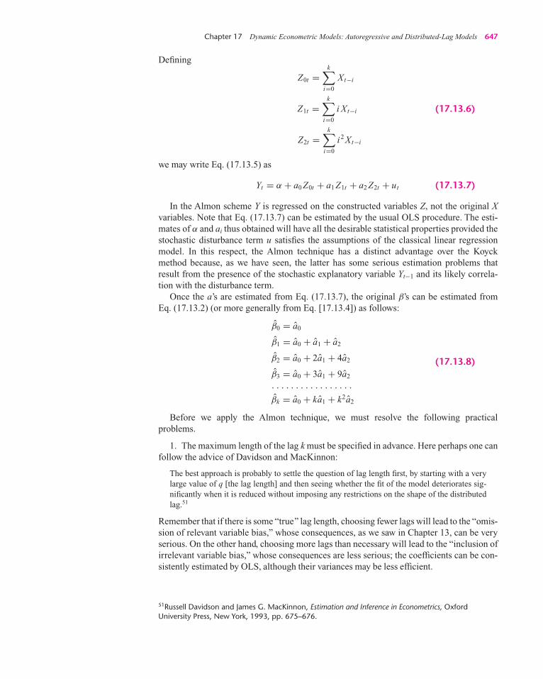
Chapter 17 Dynamic Econometric Models: Autoregressive and Distributed-Lag Models 647
Defining
Z0t =k∑
i=0
Xt−i
Z1t =k∑
i=0
i Xt−i (17.13.6)
Z2t =k∑
i=0
i2 Xt−i
we may write Eq. (17.13.5) as
Yt = α + a0 Z0t + a1 Z1t + a2 Z2t + ut (17.13.7)
In the Almon scheme Y is regressed on the constructed variables Z, not the original Xvariables. Note that Eq. (17.13.7) can be estimated by the usual OLS procedure. The esti-mates of α and ai thus obtained will have all the desirable statistical properties provided thestochastic disturbance term u satisfies the assumptions of the classical linear regressionmodel. In this respect, the Almon technique has a distinct advantage over the Koyckmethod because, as we have seen, the latter has some serious estimation problems thatresult from the presence of the stochastic explanatory variable Yt−1 and its likely correla-tion with the disturbance term.
Once the a’s are estimated from Eq. (17.13.7), the original β’s can be estimated from Eq. (17.13.2) (or more generally from Eq. [17.13.4]) as follows:
β0 = a0
β1 = a0 + a1 + a2
β2 = a0 + 2a1 + 4a2 (17.13.8)β3 = a0 + 3a1 + 9a2
. . . . . . . . . . . . . . . . .
βk = a0 + ka1 + k2a2
Before we apply the Almon technique, we must resolve the following practicalproblems.
1. The maximum length of the lag k must be specified in advance. Here perhaps one canfollow the advice of Davidson and MacKinnon:
The best approach is probably to settle the question of lag length first, by starting with a verylarge value of q [the lag length] and then seeing whether the fit of the model deteriorates sig-nificantly when it is reduced without imposing any restrictions on the shape of the distributedlag.51
Remember that if there is some “true’’ lag length, choosing fewer lags will lead to the “omis-sion of relevant variable bias,’’ whose consequences, as we saw in Chapter 13, can be veryserious. On the other hand, choosing more lags than necessary will lead to the “inclusion ofirrelevant variable bias,’’ whose consequences are less serious; the coefficients can be con-sistently estimated by OLS, although their variances may be less efficient.
51Russell Davidson and James G. MacKinnon, Estimation and Inference in Econometrics, OxfordUniversity Press, New York, 1993, pp. 675–676.
guj75772_ch17.qxd 22/08/2008 12:09 PM Page 647

648 Part Three Topics in Econometrics
One can use the Akaike or Schwarz information criterion discussed in Chapter 13 tochoose the appropriate lag length. These criteria can also be used to discuss the appropriatedegree of the polynomial in addition to the discussion in point 2.
2. Having specified k, we must also specify the degree of the polynomial m. Generally,the degree of the polynomial should be at least one more than the number of turning pointsin the curve relating βi to i. Thus, in Figure 17.7a there is only one turning point; hence asecond-degree polynomial will be a good approximation. In Figure 17.7c there are twoturning points; hence a third-degree polynomial will provide a good approximation. Apriori, however, one may not know the number of turning points, and therefore, the choiceof m is largely subjective. However, theory may suggest a particular shape in some cases.In practice, one hopes that a fairly low-degree polynomial (say, m = 2 or 3) will give goodresults. Having chosen a particular value of m, if we want to find out whether a higher-degree polynomial will give a better fit, we can proceed as follows.
Suppose we must decide between the second- and third-degree polynomials. For thesecond-degree polynomial the estimating equation is as given by Eq. (17.13.7). For thethird-degree polynomial the corresponding equation is
Yt = α + a0 Z0t + a1 Z1t + a2 Z2t + a3 Z3t + ut (17.13.9)
where Z3t = ∑ki=0 i3 Xt−i . After running regression (17.13.9), if we find that a2 is statisti-
cally significant but a3 is not, we may assume that the second-degree polynomial provides areasonably good approximation.
Alternatively, as Davidson and MacKinnon suggest, “After q [the lag length] is deter-mined, one can then attempt to determine d [the degree of the polynomial] once again start-ing with a large value and then reducing it.’’52
However, we must beware of the problem of multicollinearity, which is likely to arisebecause of the way the Z’s are constructed from the X’s, as shown in Eq. (17.13.6) (seealso Eq. [17.13.10]). As shown in Chapter 10, in cases of serious multicollinearity, a3
may turn out to be statistically insignificant, not because the true a3 is zero, but simplybecause the sample at hand does not allow us to assess the separate impact of Z3 on Y.Therefore, in our illustration, before we accept the conclusion that the third-degreepolynomial is not the correct choice, we must make sure that the multicollinearity prob-lem is not serious enough, which can be done by applying the techniques discussed inChapter 10.
3. Once m and k are specified, the Z’s can be readily constructed. For instance, if m = 2and k = 5, the Z’s are
Z0t =5∑
i=0
Xt−i = (Xt + Xt−1 + Xt−2 + Xt−3 + Xt−4 + Xt−5)
Z1t =5∑
i=0
i Xt−i = (Xt−1 + 2Xt−2 + 3Xt−3 + 4Xt−4 + 5Xt−5) (17.13.10)
Z2t =5∑
i=0
i2 Xt−i = (Xt−1 + 4Xt−2 + 9Xt−3 + 16Xt−4 + 25Xt−5)
Notice that the Z’s are linear combinations of the original X’s. Also notice why the Z’sare likely to exhibit multicollinearity.
52Ibid., pp. 675–676.
guj75772_ch17.qxd 22/08/2008 12:09 PM Page 648

Chapter 17 Dynamic Econometric Models: Autoregressive and Distributed-Lag Models 649
EXAMPLE 17.11Illustration of theAlmon Distributed-Lag Model
To illustrate the Almon technique, Table 17.8 gives data on inventories Y and sales X forthe United States for the period 1954–1999.
For illustrative purposes, assume that inventories depend on sales in the current yearand in the preceding 3 years as follows:
Yt = α + β0 Xt + β1 Xt−1 + β2 Xt−2 + β3 Xt−3 + ut (17.13.11)
Furthermore, assume that βi can be approximated by a second-degree polynomial asshown in Eq. (17.13.2). Then, following Eq. (17.13.7), we may write
Yt = α + a0 Z0t + a1 Z1t + a2 Z2t + ut (17.13.12)
where
Z0t =3∑
i=0
Xt−i = (Xt + Xt−1 + Xt−2 + Xt−3)
Z1t =3∑
i=0
i Xt−i = (Xt−1 + 2Xt−2 + 3Xt−3) (17.13.13)
Z2t =3∑
i=0
i 2 Xt−i = (Xt−1 + 4Xt−2 + 9Xt−3)
The Z variables thus constructed are shown in Table 17.8. Using the data on Y and the Z ’s,we obtain the following regression:
Y t = 25,845.06 + 1.1149Z0t − 0.3713Z1t − 0.0600Z2t
se = (6596.998) (0.5381) (1.3743) (0.4549)
t = (3.9177) (2.0718) (−0.2702) (−0.1319)(17.13.14)
R2 = 0.9755 d = 0.1643 F = 517.7656
Note: Since we are using a 3-year lag, the total number of observations has been reducedfrom 46 to 43.
(Continued )
Before proceeding to a numerical example, note the advantages of the Almon method.First, it provides a flexible method of incorporating a variety of lag structures (see Exer-cise 17.17). The Koyck technique, on the other hand, is quite rigid in that it assumes thatthe β’s decline geometrically. Second, unlike the Koyck technique, in the Almon methodwe do not have to worry about the presence of the lagged dependent variable as an ex-planatory variable in the model and the problems it creates for estimation. Finally, if asufficiently low-degree polynomial can be fitted, the number of coefficients to be esti-mated (the a’s) is considerably smaller than the original number of coefficients (the β’s).
But let us re-emphasize the problems with the Almon technique. First, the degree of thepolynomial as well as the maximum value of the lag is largely a subjective decision. Second,for reasons noted previously, the Z variables are likely to exhibit multicollinearity. Therefore,in models like Eq. (17.13.9) the estimated a’s are likely to show large standard errors (relativeto the values of these coefficients), thereby rendering one or more such coefficients statisti-cally insignificant on the basis of the conventional t test. But this does not necessarily meanthat one or more of the original β coefficients will also be statistically insignificant. (The proofof this statement is slightly involved but is suggested in Exercise 17.18.) As a result, the mul-ticollinearity problem may not be as serious as one might think. Besides, as we know, in casesof multicollinearity even if we cannot estimate an individual coefficient precisely, a linearcombination of such coefficients (the estimable function) can be estimated more precisely.
guj75772_ch17.qxd 22/08/2008 07:55 PM Page 649

650 Part Three Topics in Econometrics
TABLE 17.8 Inventories Y and Sales X, U.S. Manufacturing, and Constructed Z’s
Observation Inventory Sales Z0 Z1 Z2
1954 41,612 23,355 NA NA NA1955 45,069 26,480 NA NA NA1956 50,642 27,740 NA NA NA1957 51,871 28,736 106,311 150,765 343,8551958 50,203 27,248 110,204 163,656 378,0161959 52,913 30,286 114,010 167,940 391,8521960 53,786 30,878 117,148 170,990 397,9021961 54,871 30,922 119,334 173,194 397,2541962 58,172 33,358 125,444 183,536 427,0081963 60,029 35,058 130,216 187,836 434,9481964 63,410 37,331 136,669 194,540 446,7881965 68,207 40,995 146,742 207,521 477,7851966 77,986 44,870 158,254 220,831 505,8411967 84,646 46,486 169,682 238,853 544,8291968 90,560 50,229 182,580 259,211 594,9211969 98,145 53,501 195,086 277,811 640,0031970 101,599 52,805 203,021 293,417 672,7911971 102,567 55,906 212,441 310,494 718,8701972 108,121 63,027 225,239 322,019 748,6351973 124,499 72,931 244,669 333,254 761,8961974 157,625 84,790 276,654 366,703 828,1931975 159,708 86,589 307,337 419,733 943,7571976 174,636 98,797 343,107 474,962 1,082,1281977 188,378 113,201 383,377 526,345 1,208,2631978 211,691 126,905 425,492 570,562 1,287,6901979 242,157 143,936 482,839 649,698 1,468,8821980 265,215 154,391 538,433 737,349 1,670,3651981 283,413 168,129 593,361 822,978 1,872,2801982 311,852 163,351 629,807 908,719 2,081,1171983 312,379 172,547 658,418 962,782 2,225,3861984 339,516 190,682 694,709 1,003,636 2,339,1121985 334,749 194,538 721,118 1,025,829 2,351,0291986 322,654 194,657 752,424 1,093,543 2,510,1891987 338,109 206,326 786,203 1,155,779 2,688,9471988 369,374 224,619 820,140 1,179,254 2,735,7961989 391,212 236,698 862,300 1,221,242 2,801,8361990 405,073 242,686 910,329 1,304,914 2,992,1081991 390,905 239,847 943,850 1,389,939 3,211,0491992 382,510 250,394 969,625 1,435,313 3,340,8731993 384,039 260,635 993,562 1,458,146 3,393,9561994 404,877 279,002 1,029,878 1,480,964 3,420,8341995 430,985 299,555 1,089,586 1,551,454 3,575,0881996 436,729 309,622 1,148,814 1,639,464 3,761,2781997 456,133 327,452 1,215,631 1,745,738 4,018,8601998 466,798 337,687 1,274,316 1,845,361 4,261,9351999 470,377 354,961 1,329,722 1,921,457 4,434,093
Note: Y and X are in millions of dollars, seasonally adjusted.
Source: Economic Report of the President, 2001, Table B-57, p. 340. The Z ’s are as shown in Eq. (17.13.13).
EXAMPLE 17.11(Continued)
guj75772_ch17.qxd 22/08/2008 07:55 PM Page 650

Chapter 17 Dynamic Econometric Models: Autoregressive and Distributed-Lag Models 651
Our illustrative example may be used to point out a few additional features of the Almonlag procedure:
1. The standard errors of the a coefficients are directly obtainable from the OLS regression(17.13.14), but the standard errors of some of the β coefficients, the objective of primaryinterest, cannot be so obtained. But they can be obtained from the standard errors of theestimated a coefficients by using a well-known formula from statistics, which is given inExercise 17.18. Of course, there is no need to do this manually, for most statistical pack-ages can do this routinely. The standard errors given in Eq. (17.13.15) were obtainedfrom EViews 6.
A brief comment on the preceding results is in order. Of the three Z variables, only Z0
is individually statistically significant at the 5 percent level, but the others are not, yet theF value is so high that we can reject the null hypothesis that collectively the Z ’s have noeffect on Y. As you may suspect, this might very well be due to multicollinearity. Also, notethat the computed d value is very low. This does not necessarily mean that the residualssuffer from autocorrelation. More likely, the low d value suggests that the model we haveused is probably mis-specified. We will comment on this shortly.
From the estimated a’s given in Eq. (17.13.3), we can easily estimate the original β’seasily, as shown in Eq. (17.13.8). In the present example, the results are as follows:
β0 = a 0 = 1.1149
β1 = (a 0 + a1 + a 2) = 0.6836
β2 = (a 0 + 2a1 + 4a 2) = 0.1321(17.13.15)
β3 = (a 0 + 3a1 + 9a 2) = −0.5394
Thus, the estimated distributed-lag model corresponding to Eq. (17.13.11) is:
Yt = 25,845.0 + 1.1150X0 + 0.6836Xt−1 + 0.1321Xt−2 − 0.5394Xt−3
se = (6596.99) (0.5381) (0.4672) (0.4656) (0.5656) (17.13.16)
t = (3.9177) (2.0718) (1.4630) (0.2837) (−0.9537)
Geometrically, the estimated βi is as shown in Figure 17.8.
EXAMPLE 17.11(Continued)
FIGURE 17.8Lag structure of theillustrative example.
0.5-0.8
1.0 1.5 2.0 2.5 3.0 3.5 4.0 4.5Lag
Bet
a
-0.4
0.0
0.4
0.8
1.2
guj75772_ch17.qxd 22/08/2008 12:09 PM Page 651

652 Part Three Topics in Econometrics
2. The β’s obtained in Eq. (17.13.16) are called unrestricted estimates in the sense that noa priori restrictions are placed on them. In some situations, however, one may want toimpose the so-called endpoint restrictions on the β’s by assuming that β0 and βk (thecurrent and kth lagged coefficient) are zero. Because of psychological, institutional, ortechnical reasons, the value of the explanatory variable in the current period may nothave any impact on the current value of the regressand, thereby justifying the zero valuefor β0. By the same token, beyond a certain time the kth lagged coefficient may not haveany impact on the regressand, thus supporting the assumption that βk is zero. In ourinventory example (Example 17.11), the coefficient of Xt−3 had a negative sign, whichmay not make economic sense. Hence, one may want to constrain that coefficient tozero.53 Of course, you do not have to constrain both ends; you could put restriction onlyon the first coefficient, called near-end restriction, or on the last coefficient, calledfar-end restriction. For our inventory example, this is illustrated in Exercise 17.28.Sometimes the β’s are estimated with the restriction that their sum is 1. But one shouldnot put such restrictions mindlessly because such restrictions also affect the values ofthe other (unconstrained) lagged coefficients.
3. Since the choice of the number of lagged coefficients as well as the degree of the poly-nomial is at the discretion of the modeler, some trial and error is inevitable, the chargeof data mining notwithstanding. Here is where the Akaike and Schwarz informationcriteria discussed in Chapter 13 may come in handy.
4. Since we estimated Eq. (17.13.16) using three lags and the second-degree polynomial,it is a restricted least-squares model. Suppose we decide to use three lags but do not usethe Almon polynomial approach. That is, we estimate Eq. (17.13.11) by OLS. Whatthen? Let us first see the results:
Yt = 26,008.60 + 0.9771Xt + 1.0139X t−1 − 0.2022 Xt−2 − 0.3935Xt−3
se = (6691.12) (0.6820) (1.0920) (1.1021) (0.7186)
t = (3.8870) (1.4327) (0.9284) (−0.1835) (−0.5476)
R2 = 0.9755 d = 0.1571 F = 379.51 (17.13.17)
If you compare these results with those given in Eq. (17.13.16), you will see that the over-all R2 is practically the same, although the lagged pattern in (17.13.17) shows more of ahumped shape than that exhibited by Eq. (17.13.16). It is left to the reader to verify the R2
value from (17.13.16).As this example illustrates, one has to be careful in using the Almon distributed lag tech-
nique, as the results might be sensitive to the choice of the degree of the polynomial and/orthe number of lagged coefficients.
17.14 Causality in Economics: The Granger Causality Test54
Back in Section 1.4 we noted that, although regression analysis deals with the dependenceof one variable on other variables, it does not necessarily imply causation. In other words,the existence of a relationship between variables does not prove causality or the direction
53For a concrete application, see D. B. Batten and Daniel Thornton, “Polynomial Distributed Lags and theEstimation of the St. Louis Equation,” Review, Federal Reserve Bank of St. Louis, April 1983, pp. 13–25.54There is another test of causality that is sometimes used, the so-called Sims test of causality. Wediscuss it by way of an exercise.
guj75772_ch17.qxd 22/08/2008 07:55 PM Page 652

Chapter 17 Dynamic Econometric Models: Autoregressive and Distributed-Lag Models 653
of influence. But in regressions involving time series data, the situation may be somewhatdifferent because, as one author puts it,
. . . time does not run backward. That is, if event A happens before event B, then it is possiblethat A is causing B. However, it is not possible that B is causing A. In other words, events in thepast can cause events to happen today. Future events cannot.55 [Emphasis added.]
This is roughly the idea behind the so-called Granger causality test.56 But it should be notedclearly that the question of causality is deeply philosophical with all kinds of controversies.At one extreme are people who believe that “everything causes everything,” and at the otherextreme are people who deny the existence of causation whatsoever.57 The econometricianEdward Leamer prefers the term precedence over causality. Francis Diebold prefers theterm predictive causality. As he writes:
. . . the statement “yi causes yj” is just shorthand for the more precise, but long-winded,statement, “yi contains useful information for predicting yj (in the linear least squaressense), over and above the past histories of the other variables in the system.” To savespace, we simply say that yi causes yj.58
The Granger Test To explain the Granger test, we will consider the often asked question in macroeconomics:Is it GDP that “causes” the money supply M (GDP → M)? Or is it the money supply Mthat causes GDP (M → GDP)? (where the arrow points to the direction of causality). TheGranger causality test assumes that the information relevant to the prediction of therespective variables, GDP and M, is contained solely in the time series data on thesevariables. The test involves estimating the following pair of regressions:
GDPt =n∑
i=1
αi Mt−i +n∑
j=1
βj GDPt− j + u1t (17.14.1)
Mt =n∑
i=1
λi Mt−i +n∑
j=1
δj GDPt− j + u2t (17.14.2)
where it is assumed that the disturbances u1t and u2t are uncorrelated. In passing, note that, sincewe have two variables, we are dealing with bilateral causality. In the chapters on time serieseconometrics, we will extend this to multivariable causality through the technique of vectorautoregression (VAR).
Equation (17.14.1) postulates that current GDP is related to past values of itself as well asthat of M, and Eq. (17.14.2) postulates a similar behavior for M. Note that these regressions can
55Gary Koop, Analysis of Economic Data, John Wiley & Sons, New York, 2000, p. 175.56C. W. J. Granger, “Investigating Causal Relations by Econometric Models and Cross-Spectral Meth-ods,” Econometrica, July 1969, pp. 424–438. Although popularly known as the Granger causality test,it is appropriate to call it the Wiener–Granger causality test, for it was earlier suggested byWiener. See N. Wiener, “The Theory of Prediction,” in E. F. Beckenback, ed., Modern Mathematics forEngineers, McGraw-Hill, New York, 1956, pp. 165–190.57For an excellent discussion of this topic, see Arnold Zellner, “Causality and Econometrics,” Carnegie-Rochester Conference Series, 10, K. Brunner and A. H. Meltzer, eds., North Holland PublishingCompany, Amsterdam, 1979, pp. 9–50.58Francis X. Diebold, Elements of Forecasting, South Western Publishing, 2d ed., 2001, p. 254.
guj75772_ch17.qxd 22/08/2008 12:09 PM Page 653

654 Part Three Topics in Econometrics
be cast in growth forms, ˙GDP and M, where a dot over a variable indicates its growth rate. Wenow distinguish four cases:
1. Unidirectional causality from M to GDP is indicated if the estimated coefficients on thelagged M in Eq. (17.14.1) are statistically different from zero as a group and the set ofestimated coefficients on the lagged GDP in Eq. (17.14.2) is not statistically differentfrom zero.
2. Conversely, unidirectional causality from GDP to M exists if the set of lagged M coeffi-cients in Eq. (17.14.1) is not statistically different from zero and the set of the laggedGDP coefficients in Eq. (17.14.2) is statistically different from zero.
3. Feedback, or bilateral causality, is suggested when the sets of M and GDP coefficientsare statistically significantly different from zero in both regressions.
4. Finally, independence is suggested when the sets of M and GDP coefficients are not sta-tistically significant in either of the regressions.
More generally, since the future cannot predict the past, if variable X (Granger) causesvariable Y, then changes in X should precede changes in Y. Therefore, in a regression of Yon other variables (including its own past values) if we include past or lagged values of Xand it significantly improves the prediction of Y, then we can say that X (Granger) causes Y.A similar definition applies if Y (Granger) causes X.
The steps involved in implementing the Granger causality test are as follows. We illus-trate these steps with the GDP-money example given in Eq. (17.14.1).
1. Regress current GDP on all lagged GDP terms and other variables, if any, but do notinclude the lagged M variables in this regression. As per Chapter 8, this is therestricted regression. From this regression obtain the restricted residual sum ofsquares, RSSR.
2. Now run the regression including the lagged M terms. In the language of Chapter 8, thisis the unrestricted regression. From this regression obtain the unrestricted residual sumof squares, RSSUR.
3. The null hypothesis is H0: αi = 0, i = 1, 2, . . . , n, that is, lagged M terms do not be-long in the regression.
4. To test this hypothesis, we apply the F test given by Eq. (8.7.9), namely,
F = (RSSR − RSSUR)/m
RSSUR/(n − k)(8.7.9)
which follows the F distribution with m and (n − k) df. In the present case m is equal tothe number of lagged M terms and k is the number of parameters estimated in the unre-stricted regression.
5. If the computed F value exceeds the critical F value at the chosen level of significance, wereject the null hypothesis, in which case the lagged M terms belong in the regression. Thisis another way of saying that M causes GDP.
6. Steps 1 to 5 can be repeated to test the model (17.14.2), that is, whether GDP causes M.
Before we illustrate the Granger causality test, there are several things that need to benoted:
1. It is assumed that the two variables, GDP and M, are stationary. We have already dis-cussed the concept of stationarity in intuitive terms before and will discuss it more for-mally in Chapter 21. Sometimes taking the first differences of the variables makes themstationary, if they are not already stationary in the level form.
guj75772_ch17.qxd 22/08/2008 12:09 PM Page 654

Chapter 17 Dynamic Econometric Models: Autoregressive and Distributed-Lag Models 655
59For further details, see Wojciech W. Charemza and Derek F. Deadman, New Directions in EconometricPractice: General to Specific Modelling, Cointegration and Vector Autoregression, 3d ed., Edward ElgarPublishing, 1997, Chapter 6.60On this, see J. H. Stock and M. W. Watson, “Interpreting the Evidence on Money-Income Causality,”Journal of Econometrics, vol. 40, 1989, pp. 783–820.61R. W. Hafer, “The Role of Fiscal Policy in the St. Louis Equation,” Review, Federal Reserve Bank of St. Louis, January 1982, pp. 17–22. See his footnote 12 for the details of the procedure.
EXAMPLE 17.12Causality betweenMoney andIncome
R. W. Hafer used the Granger test to find out the nature of causality between GNP (ratherthan GDP) and M for the United States for the period 1960–I to 1980–IV. Instead of usingthe gross values of these variables, he used their growth rates, ˙GNP and M, and used fourlags of each variable in the two regressions given previously. The results were as follows:61
The null hypothesis in each case is that the variable under consideration does not“Granger-cause” the other variable.
Direction of Causality F Value Decision
M → ˙GNP 2.68 Reject˙GNP → M 0.56 Do not reject
These results suggest that the direction of causality is from money growth to GNPgrowth since the estimated F is significant at the 5 percent level; the critical F value is 2.50(for 4 and 71 df). On the other hand, there is no “reverse causation” from GNP growth tomoney growth, since the F value is statistically insignificant.
EXAMPLE 17.13Causality betweenMoney andInterest Rate inCanada
Refer to the Canadian data given in Table 17.5. Suppose we want to find out if there is anycausality between money supply and interest rate in Canada for the quarterly periods of1979–1988. To show that the Granger causality test depends critically on the number oflagged terms introduced in the model, we present below the results of the F test usingseveral (quarterly) lags. In each case, the null hypothesis is that interest rate does not(Granger-) cause money supply and vice versa.
2. The number of lagged terms to be introduced in the causality tests is an important prac-tical question. As in the case of the distributed-lag models, we may have to use the Akaikeor Schwarz information criterion to make the choice. But it should be added that thedirection of causality may depend critically on the number of lagged terms included.
3. We have assumed that the error terms entering the causality test are uncorrelated. If thisis not the case, appropriate transformation, as discussed in Chapter 12, may have to betaken.59
4. Since our interest is in testing for causality, one need not present the estimated coeffi-cients of models (17.14.1) and (17.14.2) explicitly (to save space); just the results of theF test given in Eq. (8.7.9) will suffice.
5. One has to guard against “spurious” causality. In our GDP-money example, suppose weconsider interest rate, say the short-term interest rate. It is quite possible that money“Granger-causes” the interest rate and the interest rate in turn “Granger-causes” GDP.Therefore, if we do not account for the interest rate, and find that it is money that causesGDP, then, the observed causality between GDP and money may be spurious.60 As notedpreviously, one way of dealing with this is to consider a multiple-equation system, such asvector autoregression (VAR), which we will discuss in some length in Chapter 22.
(Continued )
guj75772_ch17.qxd 22/08/2008 12:09 PM Page 655

656 Part Three Topics in Econometrics
EXAMPLE 17.14Causality betweenGDP Growth Rateand Gross SavingsRate in Nine EastAsian Countries
A study of the bilateral causality between GDP growth rate (g) and gross savings rate (s)showed the results given in Table 17.9.62 For comparison, the results for the United Statesare also presented in the table. By and large, the results presented in Table 17.9 show thatfor most East Asian countries the causality runs from the GDP growth rate to the grosssavings rate. By contrast, for the United States for the period 1950–1988 up to lag 3,causality ran in both directions, but for lags 4 and 5, the causality ran from the GDPgrowth rate to the savings rate but not the other way round.
62These results are obtained from The East Asian Miracle: Economic Growth and Public Policy, publishedfor the World Bank by Oxford University Press, 1993, p. 244.
Lagged Right-hand Lagged Right-handEconomy, Years Side Variable Economy, Years Side Variable
Years of Lags Savings Growth Years of Lags Savings Growth
Hong Kong, 1 Sig Sig Philippines, 1 NS Sig1960–88 2 Sig Sig 1950–88 2 NS Sig
3 Sig Sig 3 NS Sig4 Sig Sig 4 NS Sig5 Sig Sig 5 NS Sig
Indonesia, 1 Sig Sig Singapore, 1 NS NS1965 2 NS Sig 1960–88 2 NS NS
3 NS Sig 3 NS NS4 NS Sig 4 Sig NS5 NS Sig 5 Sig NS
Japan, 1 NS Sig Taiwan, China, 1 Sig Sig1950–88 2 NS Sig 1950–88 2 NS Sig
3 NS Sig 3 NS Sig4 NS Sig 4 NS Sig5 NS Sig 5 NS Sig
Korea, Rep. of, 1 Sig Sig Thailand, 1 NS Sig1955–88 2 NS Sig 1950–88 2 NS Sig
3 NS Sig 3 NS Sig4 NS Sig 4 NS Sig5 NS Sig 5 NS Sig
Malaysia, 1 Sig Sig United States, 1 Sig Sig1955–88 2 Sig Sig 1950–88 2 Sig Sig
3 NS NS 3 Sig Sig4 NS NS 4 NS Sig5 NS Sig 5 NS Sig
Sig: Significant; NS: Not significant.Note: Growth is real per capita GDP growth at 1985 international prices.
TABLE 17.9Tests of BivariateGranger Causalitybetween the RealPer Capita GDPGrowth Rateand the GrossSavings Rate
Source: World Bank, TheEast Asian Miracle:Economic Growth andPublic Policy, OxfordUniversity Press, NewYork, 1993, p. 244,(Table A5-2). The originalsource is Robert Summersand Alan Heston, “ThePenn World Tables (Mark 5):An Expanded Set ofInternational Comparisons,1950–88,” QuarterlyJournal of Economics,vol. 105, no. 2, 1991.
Direction of Causality Number of Lags F Value Decision
R → M 2 12.92 RejectM → R 2 3.22 RejectR → M 4 5.59 RejectM → R 4 2.45 Reject (at 7%)R → M 6 3.5163 RejectM → R 6 2.71 RejectR → M 8 1.40 Do not rejectM → R 8 1.62 Do not reject
Note these features of the preceding results of the F test: Up to six lags, there is bilateralcausality between money supply and interest rate. However, at eight lags, there is nostatistically discernible relationship between the two variables. This reinforces the pointmade earlier that the outcome of the Granger test is sensitive to the number of lags intro-duced in the model.
EXAMPLE 17.13(Continued)
guj75772_ch17.qxd 28/08/2008 10:52 AM Page 656

Chapter 17 Dynamic Econometric Models: Autoregressive and Distributed-Lag Models 657
*A Note on Causality and ExogeneityAs we will study in the chapters on simultaneous-equation models in Part 4 of this text, eco-nomic variables are often classified into two broad categories, endogenous and exogenous.Loosely speaking, endogenous variables are the equivalent of the dependent variable in thesingle-equation regression model and exogenous variables are the equivalent of the X vari-ables, or regressors, in such a model, provided the X variables are uncorrelated with the errorterm in that equation.63
Now we raise an interesting question: Suppose in a Granger causality test we find thatan X variable (Granger-) causes a Y variable without being caused by the latter (i.e., nobilateral causality). Can we then treat the X variable as exogenous? In other words, can weuse Granger causality (or noncausality) to establish exogeneity?
To answer this question, we need to distinguish three types of exogeneity: (1) weak,(2) strong, and (3) super. To keep the exposition simple, suppose we consider only two vari-ables, Yt and Xt, and further suppose we regress Yt on Xt. We say that Xt is weakly exogenousif Yt also does not explain Xt. In this case estimation and testing of the regression model canbe done, conditional on the values of Xt. As a matter of fact, going back to Chapter 2, youwill realize that our regression modeling was conditional on the values of the X variables.Xt is said to be strongly exogenous if current and lagged Y values do not explain it (i.e., nofeedback relationship). And Xt is super-exogenous if the parameters in the regression of Yon X do not change even if the X values change; that is, the parameter values are invariantto changes in the value(s) of X. If that is in fact the case, then, the famous “Lucas critique”may lose its force.64
The reason for distinguishing the three types of exogeneity is that, “In general, weakexogeneity is all that is needed for estimating and testing, strong exogeneity is necessaryfor forecasting and super exogeneity for policy analysis.”65
Returning to Granger causality, if a variable, say Y, does not cause another variable, sayX, can we then assume that the latter is exogenous? Unfortunately, the answer is notstraightforward. If we are talking about weak exogeneity, it can be shown that Grangercausality is neither necessary nor sufficient to establish exogeneity. On the other hand,Granger causality is necessary (but not sufficient) for strong exogeneity. The proofs ofthese statements are beyond the scope of this book.66 For our purpose, then, it is better to
*Optional.63Of course, if the explanatory variables include one or more lagged terms of the endogenousvariable, this requirement may not be fulfilled.64The Nobel laureate Robert Lucas put forth the proposition that existing relations between economicvariables may change when policy changes, in which case the estimated parameters from aregression model will be of little value for prediction. On this, see Oliver Blanchard, Macroeconomics,Prentice Hall, 1997, pp. 371–372.65Keith Cuthbertson, Stephen G. Hall, and Mark P. Taylor, Applied Econometric Techniques, Universityof Michigan Press, 1992, p. 100.66For a comparatively simple discussion, see G. S. Maddala, Introduction to Econometrics, 2d ed.,Macmillan, New York, 1992, pp. 394–395, and also David F. Hendry, Dynamic Econometrics, OxfordUniversity Press, New York, 1995, Chapter 5.
To conclude our discussion of Granger causality, keep in mind that the question we areexamining is whether statistically one can detect the direction of causality when temporallythere is a lead–lag relationship between two variables. If causality is established, it suggeststhat one can use a variable to better predict the other variable than simply the past historyof that other variable. In the case of the East Asian economies, it seems that we can betterpredict the gross savings rate by considering the lagged values of the GDP growth ratethan merely the lagged values of the gross savings rate.
EXAMPLE 17.14(Continued)
guj75772_ch17.qxd 22/08/2008 12:09 PM Page 657

658 Part Three Topics in Econometrics
keep the concepts of Granger causality and exogeneity separate and treat the former as auseful descriptive tool for time series data. In Chapter 19 we will discuss a test that can beused to find out if a variable can be treated as exogenous.
67For applications of these models, see Arnold C. Harberger, ed., The Demand for Durable Goods,University of Chicago Press, Chicago, 1960.
Summary andConclusions
1. For psychological, technological, and institutional reasons, a regressand may respondto a regressor(s) with a time lag. Regression models that take into account time lags areknown as dynamic or lagged regression models.
2. There are two types of lagged models: distributed-lag and autoregressive. In the former, the current and lagged values of regressors are explanatory variables. In thelatter, the lagged value(s) of the regressand appears as an explanatory variable(s).
3. A purely distributed-lag model can be estimated by OLS, but in that case there is theproblem of multicollinearity since successive lagged values of a regressor tend to becorrelated.
4. As a result, some shortcut methods have been devised. These include the Koyck, theadaptive expectations, and partial adjustment mechanisms, the first being a purelyalgebraic approach and the other two being based on economic principles.
5. A unique feature of the Koyck,adaptive expectations, and partial adjustment modelsis that they all are autoregressive in nature in that the lagged value(s) of the regressandappears as one of the explanatory variables.
6. Autoregressiveness poses estimation challenges; if the lagged regressand is correlatedwith the error term, OLS estimators of such models are not only biased but also areinconsistent. Bias and inconsistency are the case with the Koyck and the adaptiveexpectations models; the partial adjustment model is different in that it can be consis-tently estimated by OLS despite the presence of the lagged regressand.
7. To estimate the Koyck and adaptive expectations models consistently, the most popu-lar method is the method of instrumental variable. The instrumental variable is aproxy variable for the lagged regressand but with the property that it is uncorrelatedwith the error term.
8. An alternative to the lagged regression models just discussed is the Almon polynomialdistributed-lag model, which avoids the estimation problems associated with theautoregressive models. The major problem with the Almon approach, however, is thatone must prespecify both the lag length and the degree of the polynomial. There areboth formal and informal methods of resolving the choice of the lag length and thedegree of the polynomial.
9. Despite the estimation problems, which can be surmounted, the distributed andautoregressive models have proved extremely useful in empirical economics becausethey make the otherwise static economic theory a dynamic one by taking into accountexplicitly the role of time. Such models help us to distinguish between the short- andthe long-run responses of the dependent variable to a unit change in the value of theexplanatory variable(s). Thus, for estimating short- and long-run price, income,substitution, and other elasticities these models have proved to be highly useful.67
10. Because of the lags involved, distributed and/or autoregressive models raise the topicof causality in economic variables. In applied work, Granger causality modeling has
guj75772_ch17.qxd 22/08/2008 12:09 PM Page 658

Chapter 17 Dynamic Econometric Models: Autoregressive and Distributed-Lag Models 659
received considerable attention. But one has to exercise great caution in using theGranger methodology because it is very sensitive to the lag length used in the model.
11. Even if a variable (X) “Granger-causes” another variable (Y), it does not mean that X isexogenous. We distinguished three types of exogeneity—weak, strong, and super—and pointed out the importance of the distinction.
*Adapted from G. K. Shaw, op. cit., p. 26.
EXERCISES Questions17.1. Explain with a brief reason whether the following statements are true, false, or
uncertain:
a. All econometric models are essentially dynamic.
b. The Koyck model will not make much sense if some of the distributed-lag coef-ficients are positive and some are negative.
c. If the Koyck and adaptive expectations models are estimated by OLS, the esti-mators will be biased but consistent.
d. In the partial adjustment model, OLS estimators are biased in finite samples.
e. In the presence of a stochastic regressor(s) and an autocorrelated error term,the method of instrumental variables will produce unbiased as well as consistentestimates.
f. In the presence of a lagged regressand as a regressor, the Durbin–Watson d sta-tistic to detect autocorrelation is practically useless.
g. The Durbin h test is valid in both large and small samples.
h. The Granger test is a test of precedence rather than a test of causality.
17.2. Establish Eq. (17.7.2).
17.3. Prove Eq. (17.8.3).
17.4. Assume that prices are formed according to the following adaptive expectations hypothesis:
P∗t = γPt−1 + (1 − γ ) P∗
t−1
where P* is the expected price and P the actual price.
Complete the following table, assuming γ = 0.5:*
Period P* P
t − 3 100 110t − 2 125t − 1 155t 185t + 1 —
17.5. Consider the model
Yt = α + β1 X1t + β2 X2t + β3Yt−1 + vt
guj75772_ch17.qxd 22/08/2008 07:55 PM Page 659

660 Part Three Topics in Econometrics
Suppose Yt−1 and vt are correlated. To remove the correlation, suppose we use thefollowing instrumental variable approach: First regress Yt on X1t and X2t and obtainthe estimated Yt from this regression. Then regress
Yt = α + β1 X1t + β2 X2t + β3Yt−1 + vt
where Yt−1 are estimated from the first-stage regression.
a. How does this procedure remove the correlation between Yt−1 and vt in the orig-inal model?
b. What are the advantages of the recommended procedure over the Liviatanapproach?
*17.6. a. Establish (17.4.8).
b. Evaluate the median lag for λ = 0.2, 0.4, 0.6, 0.8.
c. Is there any systematic relationship between the value of λ and the value of themedian lag?
17.7. a. Prove that for the Koyck model, the mean lag is as shown in Eq. (17.4.10).
b. If λ is relatively large, what are its implications?
17.8. Using the formula for the mean lag given in Eq. (17.4.9), verify the mean lag of10.959 quarters reported in the illustration of Table 17.1.
17.9. Suppose
Mt = α + β1Y ∗t + β2 R∗
t + ut
where M = demand for real cash balances, Y* = expected real income, and R* =expected interest rate. Assume that expectations are formulated as follows:
Y ∗t = γ1Yt + (1 − γ1)Y ∗
t−1
R∗t = γ2 Rt + (1 − γ2)R∗
t−1
where γ1 and γ2 are coefficients of expectation, both lying between 0 and 1.
a. How would you express Mt in terms of the observable quantities?
b. What estimation problems do you foresee?
*17.10. If you estimate Eq. (17.7.2) by OLS, can you derive estimates of the original pa-rameters? What problems do you foresee? (For details, see Roger N. Waud.)†
17.11. Serial correlation model. Consider the following model:
Yt = α + βXt + ut
Assume that ut follows the Markov first-order autoregressive scheme given inChapter 12, namely,
ut = ρut−1 + εt
where ρ is the coefficient of (first-order) autocorrelation and where εt satisfies allthe assumptions of the classical OLS. Then, as shown in Chapter 12, the model
Yt = α(1 − ρ) + β(Xt − ρXt−1) + ρYt−1 + εt
will have a serially independent error term, making OLS estimation possible. Butthis model, called the serial correlation model, very much resembles the Koyck,
*Optional.†“Misspecification in the ‘Partial Adjustment’ and ‘Adaptive Expectations’ Models,” InternationalEconomic Review, vol. 9, no. 2, June 1968, pp. 204–217.
guj75772_ch17.qxd 22/08/2008 12:09 PM Page 660

Chapter 17 Dynamic Econometric Models: Autoregressive and Distributed-Lag Models 661
adaptive expectations, and partial adjustment models. How would you know in anygiven situation which of the preceding models is appropriate?*
17.12. Consider the Koyck (or, for that matter, the adaptive expectations) model given inEq. (17.4.7), namely,
Yt = α(1 − λ) + β0 Xt + λYt−1 + (ut − λut−1)
Suppose in the original model ut follows the first-order autoregressive schemeut − ρu1−t = εt , where ρ is the coefficient of autocorrelation and where εt satis-fies all the classical OLS assumptions.
a. If ρ = λ, can the Koyck model be estimated by OLS?
b. Will the estimates thus obtained be unbiased? Consistent? Why or why not?
c. How reasonable is it to assume that ρ = λ?
17.13. Triangular, or arithmetic, distributed-lag model.† This model assumes that thestimulus (explanatory variable) exerts its greatest impact in the current time periodand then declines by equal decrements to zero as one goes into the distant past.Geometrically, it is shown in Figure 17.9. Following this distribution, suppose werun the following succession of regressions:
Yt = α + β
(2Xt + Xt−1
3
)
Yt = α + β
(3Xt + 2Xt−1 + Xt−2
6
)
Yt = α + β
(4Xt + 3Xt−1 + 2Xt−2 + Xt−1
10
)
etc., and choose the regression that gives the highest R2 as the “best’’ regression.Comment on this strategy.
*For a discussion of the serial correlation model, see Zvi Griliches, “Distributed Lags: A Survey,”Econometrica, vol. 35, no. 1, January 1967, p. 34.†This model was proposed by Irving Fisher in “Note on a Short-Cut Method for Calculating Distrib-uted Lags,” International Statistical Bulletin, 1937, pp. 323–328.
0Time
kβFIGURE 17.9Triangular orarithmetic lag scheme(Fisher’s).
guj75772_ch17.qxd 22/08/2008 12:09 PM Page 661

662 Part Three Topics in Econometrics
17.14. From the quarterly data for the period 1950–1960, F. P. R. Brechling obtained thefollowing demand function for labor for the British economy (the figures in paren-theses are standard errors):*
Et = 14.22 + 0.172Qt − 0.028t − 0.0007t2 − 0.297Et−1
(2.61) (0.014) (0.015) (0.0002) (0.033)
R2 = 0.76 d = 1.37
where Et = (Et − Et−1)Q = outputt = time
The preceding equation was based on the assumption that the desired level of em-ployment E∗
t is a function of output, time, and time squared and on the hypothesisthat Et − Et−1 = δ(E∗
t − Et−1), where δ, the coefficient of adjustment, liesbetween 0 and 1.
a. Interpret the preceding regression.
b. What is the value of δ?
c. Derive the long-run demand function for labor from the estimated short-rundemand function.
d. How would you test for serial correlation in the preceding model?
17.15. In studying the farm demand for tractors, Griliches used the following model:†
T ∗t = αXβ1
1,t−1 Xβ22,t−1
where T* = desired stock of tractorsX1 = relative price of tractorsX2 = interest rate
Using the stock adjustment model, he obtained the following results for the period1921–1957:
log Tt = constant − 0.218 log X1,t−1 − 0.855 log X2,t−1 + 0.864 log Tt−1
(0.051) (0.170) (0.035)
R2 = 0.987
where the figures in the parentheses are the estimated standard errors.
a. What is the estimated coefficient of adjustment?
b. What are the short- and long-run price elasticities?
c. What are the corresponding interest elasticities?
d. What are the reasons for high or low rate of adjustment in the present model?
17.16. Whenever the lagged dependent variable appears as an explanatory variable, the R2
is usually much higher than when it is not included. What are the reasons for thisobservation?
*F. P. R. Brechling, “The Relationship between Output and Employment in British ManufacturingIndustries,” Review of Economic Studies, vol. 32, July 1965.†Zvi Griliches, “The Demand for a Durable Input: Farm Tractors in the United States, 1921–1957,” inArnold C. Harberger, ed., The Demand for Durable Goods, University of Chicago Press, Chicago, 1960.
guj75772_ch17.qxd 22/08/2008 12:09 PM Page 662

Chapter 17 Dynamic Econometric Models: Autoregressive and Distributed-Lag Models 663
17.17. Consider the lag patterns in Figure 17.10. What degree polynomials would you fitto the lag structures and why?
17.18. Consider Eq. (17.13.4):
βi = a0 + a1i + a2i2 + · · · + amim
To obtain the variance of βi from the variances of ai , we use the following formula:
var (βi ) = var (a0 + a1i + a2i2 + · · · + amim)
=m∑
j=0
i2 j var (aj ) + 2∑j<p
i ( j+p)cov (aj ap)
a. Using the preceding formula, find the variance of βi expressed as
βi = a0 + a1i + a2i2
βi = a0 + a1i + a2i2 + a3i3
b. If the variances of ai are large relative to themselves, will the variance of βi belarge also? Why or why not?
17.19. Consider the following distributed-lag model:
Yt = α + β0 Xt + β1 Xt−1 + β2 Xt−2 + β3 Xt−3 + β4 Xt−4 + ut
×
×
×
××××
××××
× ××
××× ×
××× × ×
××
×
××
××
××
××
×
××
××
××
××
××
××
i00
00
Lag Lag
Time Time
×
×
×
×
×
×
×
××
iβiβ
iβ iβ
i
ii
FIGURE 17.10Hypothetical lagstructures.
guj75772_ch17.qxd 22/08/2008 12:09 PM Page 663

664 Part Three Topics in Econometrics
iβ
kβi
0 1 2 3
Lag
FIGURE 17.11Inverted V distributed-lag model.
*See his article, “The Demand for Capital Goods by Manufacturers: A Study of Quarterly Time Series,”Econometrica, vol. 30, no. 3, July 1962, pp. 407–423.
Assume that βi can be adequately expressed by the second-degree polynomial asfollows:
βi = a0 + a1i + a2i2
How would you estimate the β’s if we want to impose the restriction thatβ0 = β4 = 0?
17.20. The inverted V distributed-lag model. Consider the k-period finite distributed-lagmodel
Yt = α + β0 Xt + β1 Xt−1 + β2 Xt−2 + · · · + βk Xt−k + ut
F. DeLeeuw has proposed the structure for the β’s as in Figure 17.11, where the β’sfollow the inverted V shape. Assuming for simplicity that k (the maximum lengthof the lag) is an even number, and further assuming that β0 and βk are zero,DeLeeuw suggests the following scheme for the β’s:*
βi = iβ 0 ≤ i ≤ k
2
= (k − i)βk
2≤ i < k
How would you use the DeLeeuw scheme to estimate the parameters of the pre-ceding k-period distributed-lag model?
17.21. Refer to Exercise 12.15. Since the d value shown there is of little use in detecting(first-order) autocorrelation (why?), how would you test for autocorrelation in thiscase?
Empirical Exercises17.22. Consider the following model:
Y ∗i = α + β0 Xt + ut
where Y ∗ = desired, or long-run, business expenditure for new plant and equip-ment, Xt = sales, and t = time. Using the stock adjustment model, estimate the
guj75772_ch17.qxd 22/08/2008 07:55 PM Page 664

Chapter 17 Dynamic Econometric Models: Autoregressive and Distributed-Lag Models 665
parameters of the long- and short-run demand function for expenditure on newplant and equipment given in Table 17.10.
How would you find out if there is serial correlation in the data?
17.23. Use the data of Exercise 17.22 but consider the following model:
Y ∗i = β0 Xβ1
t eut
Using the stock adjustment model (why?), estimate the short- and long-run elastic-ities of expenditure on new plant and equipment with respect to sales. Compareyour results with those for Exercise 17.22. Which model would you choose andwhy? Is there serial correlation in the data? How do you know?
17.24. Use the data of Exercise 17.22 but assume that
Yt = α + βX∗t + ut
where X∗t are the desired sales. Estimate the parameters of this model and compare
the results with those obtained in Exercise 17.22. How would you decide which isthe appropriate model? On the basis of the h statistic, would you conclude thereis serial correlation in the data?
17.25. Suppose someone convinces you that the relationship between business expendi-ture for new plant and equipment and sales is as follows:
Y ∗t = α + βX∗
t + ut
where Y ∗ is desired expenditure and X∗ is desired or expected sales. Use the datagiven in Exercise 17.22 to estimate this model and comment on your results.
17.26. Using the data given in Exercise 17.22, determine whether plant expenditureGranger-causes sales or whether sales Granger-cause plant expenditure. Use up tosix lags and comment on your results. What important conclusion do you drawfrom this exercise?
17.27. Assume that sales in Exercise 17.22 has a distributed-lag effect on expenditure onplant and equipment. Fit a suitable Almon lag model to the data.
17.28. Reestimate Eq. (17.13.16) imposing (1) near-end restriction, (2) far-end restriction,and (3) both end restrictions and compare your results given in Eq. (17.13.16).What general conclusion do you draw?
TABLE 17.10Investment in FixedPlant and Equipmentin Manufacturing Yand ManufacturingSales X2 in Billions ofDollars, SeasonallyAdjusted,United States,1970–1991
Source: Economic Report ofthe President, 1993. Data onY from Table B-52, p. 407;data on X2 from Table 8-53,p. 408.
Year Plant Expenditure, Y Sales, X2 Year Plant Expenditure, Y Sales, X2
1970 36.99 52.805 1981 128.68 168.1291971 33.60 55.906 1982 123.97 163.3511972 35.42 63.027 1983 117.35 172.5471973 42.35 72.931 1984 139.61 190.6821974 52.48 84.790 1985 152.88 194.5381975 53.66 86.589 1986 137.95 194.6571976 58.53 98.797 1987 141.06 206.3261977 67.48 113.201 1988 163.45 223.5411978 78.13 126.905 1989 183.80 232.7241979 95.13 143.936 1990 192.61 239.4591980 112.60 154.391 1991 182.81 235.142
guj75772_ch17.qxd 22/08/2008 12:09 PM Page 665

666 Part Three Topics in Econometrics
17.29. Table 17.11 gives data on private fixed investment in information processing andequipment (Y, in billions of dollars), sales in total manufacturing and trade (X2, inmillions of dollars), and interest rate (X3, Moody’s Aaa corporate bond rate, per-cent); data on Y and X2 are seasonally adjusted.
a. Test for bilateral causality between Y and X2, paying careful attention to the laglength.
b. Test for bilateral causality between Y and X3, again paying careful attention to the laglength.
c. To allow for the distributed lag effect of sales on investment, suppose you decideto use the Almon lag technique. Show the estimated model, after paying due at-tention to the length of the lag as well as the degree of the polynomial.
17.30. Table 17.12 gives data on indexes of real compensation per hour (Y) and output perhour (X2), with both indexes to base 1992 = 100, in the business sector of the U.S.economy for the period 1960–1999, as well as the civilian unemployment rate (X3)for the same period.
a. How would you decide whether it is wage compensation that determines laborproductivity or the other way round?
b. Develop a suitable model to test your conjecture in (a), providing the usual statistics.
c. Do you think the unemployment rate has any effect on wage compensation, and ifso, how would you take that into account? Show the necessary statistical analysis.
TABLE 17.11 Investments, Sales, and Interest Rate, United States, 1960–1999
Observation Investment Sales Interest Observation Investment Sales Interest
1960 4.9 60,827 4.41 1980 69.6 327,233 11.941961 5.2 61,159 4.35 1981 82.4 355,822 14.171962 5.7 65,662 4.33 1982 88.9 347,625 13.791963 6.5 68,995 4.26 1983 100.8 369,286 12.041964 7.3 73,682 4.40 1984 121.7 410,124 12.711965 8.5 80,283 4.49 1985 130.8 422,583 11.371966 10.6 87,187 5.13 1986 137.6 430,419 9.021967 11.2 90,820 5.51 1987 141.9 457,735 9.381968 11.9 96,685 6.18 1988 155.9 497,157 9.711969 14.6 105,690 7.03 1989 173.0 527,039 9.261970 16.7 108,221 8.04 1990 176.1 545,909 9.321971 17.3 116,895 7.39 1991 181.4 542,815 8.771972 19.3 131,081 7.21 1992 197.5 567,176 8.141973 23.0 153,677 7.44 1993 215.0 595,628 7.221974 26.8 177,912 8.57 1994 233.7 639,163 7.961975 28.2 182,198 8.83 1995 262.0 684,982 7.591976 32.4 204,150 8.43 1996 287.3 718,113 7.371977 38.6 229,513 8.02 1997 325.2 753,445 7.261978 48.3 260,320 8.73 1998 367.4 779,413 6.531979 58.6 297,701 9.63 1999 433.0 833,079 7.04
Notes: Investment = private fixed investment in information processing equipment and software, billions of dollars, seasonally adjusted.Sales = sales in total manufacturing and trade, millions of dollars, seasonally adjusted.
Interest = Moody’s Aaa corporate bond rate, %.
Source: Economic Report of the President, 2001, Tables B-18, B-57, and B-73.
guj75772_ch17.qxd 22/08/2008 12:09 PM Page 666

Chapter 17 Dynamic Econometric Models: Autoregressive and Distributed-Lag Models 667
17.31. In a test of Granger causality, Christopher Sims exploits the fact that the futurecannot cause the present.* To decide whether a variable Y causes a variable X, Simssuggests estimating the following pair of equations:
Yt = α1 +i=n∑i=1
βi Xt−i +i=m∑i=1
γi Yt−i +i=p∑i=1
λi Xt+i + u1t (1)
Xt = α2 +i=n∑i=1
δi Xt−i +i=m∑i=1
θi Yt−i +i=p∑i=1
ωi Yt+i + u2t (2)
These regressions include the lagged, current, and future, or lead, values of theregressors; terms such as Xt+1, Xt+2, etc., are called lead terms.
If Y is to Granger-cause X, then there must be some relationship between Y andthe lead, or future, values of X. Therefore, instead of testing that βi = 0, we shouldtest λi = 0 in Eq. (1). If we reject this hypothesis, the causality then runs from Yto X, and not from X to Y, because the future cannot cause the present. Similar com-ments apply to Equation (2).
TABLE 17.12 Compensation, Productivity and Unemployment Rate, United States, 1960–1999
Observation COMP PRODUCT UNRate Observation COMP PRODUCT UNRate
1960 60.0 48.8 5.5 1980 89.5 80.4 7.11961 61.8 50.6 6.7 1981 89.5 82.0 7.61962 63.9 52.9 5.5 1982 90.9 81.7 9.71963 65.4 55.0 5.7 1983 91.0 84.6 9.61964 67.9 57.5 5.2 1984 91.3 87.0 7.51965 69.4 59.6 4.5 1985 92.7 88.7 7.21966 71.9 62.0 3.8 1986 95.8 91.4 7.01967 73.8 63.4 3.8 1987 96.3 91.9 6.21968 76.3 65.4 3.6 1988 97.3 93.0 5.51969 77.4 65.7 3.5 1989 95.9 93.9 5.31970 78.9 67.0 4.9 1990 96.5 95.2 5.61971 80.4 69.9 5.9 1991 97.5 96.3 6.81972 82.7 72.2 5.6 1992 100.0 100.0 7.51973 84.5 74.5 4.9 1993 99.9 100.5 6.91974 83.5 73.2 5.6 1994 99.7 101.9 6.11975 84.4 75.8 8.5 1995 99.3 102.6 5.61976 86.8 78.5 7.7 1996 99.7 105.4 5.41977 87.9 79.8 7.1 1997 100.4 107.6 4.91978 89.5 80.7 6.1 1998 104.3 110.5 4.51979 89.7 80.7 5.8 1999 107.3 114.0 4.2
Notes: COMP = index of real compensation per hour (1992 = 100).PRODUCT = index of output per hour (1992 = 100).
UNRate = civilian unemployment rate, %.
Source: Economic Report of the President, 2001, Table B-49, p. 332.
*C. A. Sims, “Money, Income, and Causality,” American Economic Review, vol. 62, 1972, pp. 540–552.
guj75772_ch17.qxd 22/08/2008 12:09 PM Page 667

668 Part Three Topics in Econometrics
To carry out the Sims test, we estimate Eq. (1) without the lead terms (call itrestricted regression) and then estimate Eq. (1) with the lead terms (call itunrestricted regression). Then we carry out the F test as indicated in Equation(8.7.9). If the F statistic is significant (say, at the 5% level), then we conclude thatit is Y that Granger-causes X. Similar comments apply to Equation (2).
Which test do we choose—Granger or Sims? We can apply both tests.* The onefactor that is in favor of the Granger test is that it uses fewer degrees of freedom
TABLE 17.13Macroeconomic Datafor the GreekEconomy, 1960–1995
Source: H. R. Seddighi, K. A.Lawler, and A. V. Katos,Econometrics: A PracticalApproach, Routledge,London, 2000, p. 158.
Year PC PDI Grossinv GNP LTI
1960 107808 117179 29121 145458 81961 115147 127599 31476 161802 81962 120050 135007 34128 164674 81963 126115 142128 35996 181534 8.251964 137192 159649 43445 196586 91965 147707 172756 49003 214922 91966 157687 182366 50567 228040 91967 167528 195611 49770 240791 91968 179025 204470 60397 257226 8.751969 190089 222638 71653 282168 81970 206813 246819 70663 304420 81971 217212 269249 80558 327723 81972 232312 297266 92977 356886 81973 250057 335522 100093 383916 91974 251650 310231 74500 369325 11.831975 266884 327521 74660 390000 11.881976 281066 350427 79750 415491 11.51977 293928 366730 85950 431164 121978 310640 390189 91100 458675 13.461979 318817 406857 99121 476048 16.711980 319341 401942 92705 485108 21.251981 325851 419669 85750 484259 21.331982 338507 421716 84100 483879 20.51983 339425 417930 83000 481198 20.51984 345194 434696 78300 490881 20.51985 358671 456576 82360 502258 20.51986 361026 439654 77234 507199 20.51987 365473 438454 73315 505713 21.821988 378488 476345 79831 529460 22.891989 394942 492334 87873 546572 23.261990 403194 495939 96139 546982 27.621991 412458 513173 91726 566586 29.451992 420028 502520 93140 568582 28.711993 420585 523066 91292 569724 28.561994 426893 520728 93073 579846 27.441995 433723 518407 98470 588691 23.05
Note: All nominal data are expressed at constant market prices of year 1970 in millions of drachmas. Private disposable income is deflatedby the consumption price deflator.
*The choice between Granger and Sims causality tests is not clear. For further discussion of thesetests, see G. Chamberlain, “The General Equivalence of Granger and Sims Causality,” Econometrica,vol. 50, 1982, pp. 569–582.
guj75772_ch17.qxd 22/08/2008 07:55 PM Page 668

Chapter 17 Dynamic Econometric Models: Autoregressive and Distributed-Lag Models 669
because it does not use the lead terms. If the sample is not sufficiently large, we willhave to use the Sims test cautiously.
Refer to the data given in Exercise 12.34. For pedagogical purposes, apply theSims test of causality to determine whether it is sales that causes plant expenditureor vice versa. Use the last four years’ data as the lead terms in your analysis.
17.32. Table 17.13 gives some macroeconomic data for the Greek economy for the years1960–1995.
Consider the following consumption function:
ln PC∗t = β1 + β2 ln PDIt + β3LTIt + ut
Where PCt* = real desired private consumption expenditure at time t; PDIt = real
private disposable income at time t; LTIt = long-term interest rate at time t; and lnstands for natural logarithm.
a. From the data given in Table 17.13, estimate the previous consumption func-tion, stating clearly how you measured the real desired private consumptionexpenditure.
b. What econometric problems did you encounter in estimating the preceding con-sumption function? How did you resolve them? Explain fully.
17.33. Using the data in Table 17.13, develop a suitable model to explain the behavior ofgross real investment in the Greek economy for the period 1960–1995. Look up anytextbook on macroeconomics for the accelerator model of investment.
Appendix 17A
17A.1 The Sargan Test for the Validity of Instruments
Suppose we use an instrumental variable(s) to replace an explanatory variable(s) that is correlatedwith the error term. How valid is the instrumental variable(s), that is, how do we know that the in-struments chosen are independent of the error term? Sargan has developed a statistic, dubbed SARG,to test the validity of the instruments used in instrumental variable(s) (IV).* The steps involved inSARG are as follows:†
1. Divide the variables included in a regression equation into two groups, those that are independentof the error term (say, X1, X2, . . . , Xp) and those that are not independent of the error term (say,Z1, Z2, . . . , Zq).
2. Let W1, W2, . . . , Ws be the instruments chosen for the Z variables in 1, where s > q.
3. Estimate the original regression, replacing the Z’s by the W’s, that is, estimate the originalregression by IV and obtain the residuals, say, u.
4. Regress u on a constant, all the X variables and all the W variables but exclude all the Z variables.Obtain R2 from this regression.
5. Now compute the SARG statistic, defined as:
SARG = (n − k)R2 ∼ χ2s−q (17A.1.1)
*J. D. Sargan, “Wages and Prices in the United Kingdom: A Study in Econometric Methodology,” in P. E. Hart, G. Mills, and J. K. Whitaker (eds.) Econometric Analysis for National Economic Planning,Butterworths, London, 1964.†The following discussion leans on H. R. Seddighi, K. A. Lawler, and A. V. Katos, Econometrics: A Practical Approach, Routledge, New York, 2000, pp. 155–156.
guj75772_ch17.qxd 22/08/2008 07:55 PM Page 669

670 Part Three Topics in Econometrics
Where n = the number of observations and k is the number of coefficients in the originalregression equation. Under the null hypothesis that the instruments are exogenous, Sargan hasshown the SARG test asymptotically has the χ2 distribution with (s − q) degrees of freedom,where s is the number of instruments (i.e., the variables in W) and q is the number of regressors inthe original equation. If the computed chi-square value in an application is statistically significant,we reject the validity of the instruments. If it is not statistically significant, we can accept thechosen instrument as valid. It should be emphasized that s > q , that is, the number of instrumentsmust be greater than q. If that is not the case (i.e., s ≤ q), the SARG test is not valid.
6. The null hypothesis is that all (W ) instruments are valid. If the computed chi-square exceeds thecritical chi-square value, we reject the null hypothesis, which means that at least one instrumentis correlated with the error term and therefore the IV estimates based on the chosen instrumentsare not valid.
guj75772_ch17.qxd 22/08/2008 12:09 PM Page 670

Part
A casual look at the published empirical work in business and economics will reveal thatmany economic relationships are of the single-equation type. That is why we devoted thefirst three parts of this book to the discussion of single-equation regression models. In suchmodels, one variable (the dependent variable Y ) is expressed as a linear function of one ormore other variables (the explanatory variables, the X ’s). In such models an implicitassumption is that the cause-and-effect relationship, if any, between Y and the X ’s is unidi-rectional: The explanatory variables are the cause and the dependent variable is the effect.
However, there are situations where there is a two-way flow of influence among economicvariables; that is, one economic variable affects another economic variable(s) and is, in turn,affected by it (them). Thus, in the regression of money M on the rate of interest r, the single-equation methodology assumes implicitly that the rate of interest is fixed (say, by the FederalReserve System) and tries to find out the response of money demanded to the changes in thelevel of the interest rate. But what happens if the rate of interest depends on the demand formoney? In this case, the conditional regression analysis made in this book thus far maynot be appropriate because now M depends on r and r depends on M. Thus, we need toconsider two equations, one relating M to r and another relating r to M. And this leads usto consider simultaneous-equation models, models in which there is more than one regres-sion equation, one for each interdependent variable.
In Part 4 we present a very elementary and often heuristic introduction to the complexsubject of simultaneous-equation models, the details being left for the references.
In Chapter 18, we provide several examples of simultaneous-equation models and showwhy the method of ordinary least squares considered previously is generally inapplicable inestimating the parameters of each of the equations in the model.
In Chapter 19, we consider the so-called identification problem. If in a system of si-multaneous equations containing two or more equations it is not possible to obtain numer-ical values of each parameter in each equation because the equations are observationallyindistinguishable, or look too much like one another, then we have the identification
4Simultaneous-Equation Models and Time SeriesEconometrics
guj75772_ch18.qxd 28/08/2008 07:32 PM Page 671

672 Part Four Simultaneous-Equation Models and Time Series Econometrics
problem. Thus, in the regression of quantity Q on price P, is the resulting equation a de-mand function or a supply function (for Q and P enter into both functions)? Therefore, ifwe have data on Q and P only and no other information, it will be difficult if not impossi-ble to identify the regression as the demand or supply function. It is essential to resolve theidentification problem before we proceed to estimation because if we do not know what weare estimating, estimation per se is meaningless. In Chapter 19 we offer various methods ofsolving the identification problem.
In Chapter 20, we consider several estimation methods that are designed specifically forestimating the simultaneous-equation models and consider their merits and limitations.
guj75772_ch18.qxd 28/08/2008 06:21 PM Page 672

673
Chapter 18Simultaneous-EquationModelsIn this and the following two chapters we discuss the simultaneous-equation models. Inparticular, we discuss their special features, their estimation, and some of the statisticalproblems associated with them.
18.1 The Nature of Simultaneous-Equation Models
In Parts 1 to 3 of this text we were concerned exclusively with single-equation models, i.e.,models in which there was a single dependent variable Y and one or more explanatory vari-ables, the X ’s. In such models the emphasis was on estimating and/or predicting the aver-age value of Y conditional upon the fixed values of the X variables. The cause-and-effectrelationship, if any, in such models therefore ran from the X ’s to the Y.
But in many situations, such a one-way or unidirectional cause-and-effect relationship isnot meaningful. This occurs if Y is determined by the X ’s, and some of the X ’s are, in turn,determined by Y. In short, there is a two-way, or simultaneous, relationship between Y and(some of) the X ’s, which makes the distinction between dependent and explanatory vari-ables of dubious value. It is better to lump together a set of variables that can be determinedsimultaneously by the remaining set of variables—precisely what is done in simultaneous-equation models. In such models there is more than one equation—one for each of themutually, or jointly, dependent or endogenous variables.1 And unlike the single-equationmodels, in the simultaneous-equation models one may not estimate the parameters of asingle equation without taking into account information provided by other equations in thesystem.
What happens if the parameters of each equation are estimated by applying, say, themethod of ordinary least squares (OLS), disregarding other equations in the system? Recallthat one of the crucial assumptions of the method of OLS is that the explanatory X variablesare either nonstochastic or, if stochastic (random), distributed independently of the sto-chastic disturbance term. If neither of these conditions is met, then, as shown later, theleast-squares estimators are not only biased but also inconsistent; that is, as the sample size
1In the context of the simultaneous-equation models, the jointly dependent variables are calledendogenous variables and the variables that are truly nonstochastic or can be so regarded arecalled the exogenous, or predetermined, variables. (More on this in Chapter 19.)
guj75772_ch18.qxd 28/08/2008 06:21 PM Page 673

674 Part Four Simultaneous-Equation Models and Time Series Econometrics
increases indefinitely, the estimators do not converge to their true (population) values.Thus, in the following hypothetical system of equations,2
Y1i = β10 + β12Y2i + γ11 X1i + u1i (18.1.1)
Y2i = β20 + β21Y1i + γ21 X1i + u2i (18.1.2)
where Y1 and Y2 are mutually dependent, or endogenous, variables and X1 is an exogenousvariable and where u1 and u2 are the stochastic disturbance terms, the variables Y1 and Y2
are both stochastic. Therefore, unless it can be shown that the stochastic explanatory vari-able Y2 in Eq. (18.1.1) is distributed independently of u1 and the stochastic explanatoryvariable Y1 in Eq. (18.1.2) is distributed independently of u2, application of the classicalOLS to these equations individually will lead to inconsistent estimates.
In the remainder of this chapter we give a few examples of simultaneous-equation mod-els and show the bias involved in the direct application of the least-squares method to suchmodels. After discussing the so-called identification problem in Chapter 19, in Chapter 20we discuss some of the special methods developed to handle the simultaneous-equationmodels.
18.2 Examples of Simultaneous-Equation Models
2These economical but self-explanatory notations will be generalized to more than two equations inChapter 19.
EXAMPLE 18.1Demand-and-Supply Model
As is well known, the price P of a commodity and the quantity Q sold are determined bythe intersection of the demand-and-supply curves for that commodity. Thus, assuming forsimplicity that the demand-and-supply curves are linear and adding the stochastic distur-bance terms u1 and u2, we may write the empirical demand-and-supply functions as:
Demand function: Qdt = α0 + α1 Pt + u1t α1 < 0 (18.2.1)
Supply function: Qst = β0 + β1 Pt + u2t β1 > 0 (18.2.2)
Equilibrium condition: Qdt = Qs
t
where Qd = quantity demandedQs = quantity supplied
t = time
and the α’s and β’s are the parameters. A priori, α1 is expected to be negative (down-ward-sloping demand curve), and β1 is expected to be positive (upward-sloping supplycurve).
Now it is not too difficult to see that P and Q are jointly dependent variables. If, forexample, u1t in Eq. (18.2.1) changes because of changes in other variables affecting Qd
t(such as income, wealth, and tastes), the demand curve will shift upward if u1t is positiveand downward if u1t is negative. These shifts are shown in Figure 18.1.
As the figure shows, a shift in the demand curve changes both P and Q. Similarly, achange in u2t (because of strikes, weather, import or export restrictions, etc.) will shiftthe supply curve, again affecting both P and Q. Because of this simultaneous dependencebetween Q and P, u1t and Pt in Eq. (18.2.1) and u2t and Pt in Eq. (18.2.2) cannot beindependent. Therefore, a regression of Q on P as in Eq. (18.2.1) would violate animportant assumption of the classical linear regression model, namely, the assumption ofno correlation between the explanatory variable(s) and the disturbance term.
guj75772_ch18.qxd 28/08/2008 06:21 PM Page 674

Chapter 18 Simultaneous-Equation Models 675
EXAMPLE 18.2Keynesian Modelof IncomeDetermination
Consider the simple Keynesian model of income determination:
Consumption function: Ct = β0 + β1Yt + ut 0 < β1 < 1 (18.2.3)
Income identity: Yt = C t + It ( = S t) (18.2.4)
where C = consumption expenditureY = incomeI = investment (assumed exogenous)S = savingst = timeu = stochastic disturbance term
β0 and β1 = parameters
The parameter β1 is known as the marginal propensity to consume (MPC) (the amountof extra consumption expenditure resulting from an extra dollar of income). From eco-nomic theory, β1 is expected to lie between 0 and 1. Equation (18.2.3) is the (stochastic)consumption function; and Eq. (18.2.4) is the national income identity, signifying that totalincome is equal to total consumption expenditure plus total investment expenditure, it
P
Pri
ce P0
0
Quantity
Q0
D0
S
P
Pri
ce P0
0
Quantity
Q0
D0
S
Q Q
D1
Q1
P1
PP
rice P0
0 Q0
D0
S
QD1
Q1
P1
Quantity
FIGURE 18.1 Interdependence of price and quantity.
(Continued)
EXAMPLE 18.1(Continued)
guj75772_ch18.qxd 28/08/2008 06:21 PM Page 675

676 Part Four Simultaneous-Equation Models and Time Series Econometrics
being understood that total investment expenditure is equal to total savings. Diagrammat-ically, we have Figure 18.2.
From the postulated consumption function and Figure 18.2 it is clear that C and Yare interdependent and that Yt in Eq. (18.2.3) is not expected to be independent of thedisturbance term because when ut shifts (because of a variety of factors subsumed in theerror term), then the consumption function also shifts, which, in turn, affects Yt. Therefore,once again the classical least-squares method is inapplicable to Eq. (18.2.3). If applied, theestimators thus obtained will be inconsistent, as we shall show later.
EXAMPLE 18.2(Continued)
National income
Con
sum
pti
on, i
nve
stm
ent
C,I
Y
Y = C + I
C + I
C = 0 +
1Y
45º
0
β β
FIGURE 18.2Keynesian modelof incomedetermination.
EXAMPLE 18.3Wage–PriceModels
Consider the following Phillips-type model of money-wage and price determination:
Wt = α0 + α1UNt + α2 P t + u1t (18.2.5)
P t = β0 + β1Wt + β2 R t + β3Mt + u2t (18.2.6)
where W = rate of change of money wagesUN = unemployment rate, %
P = rate of change of pricesR = rate of change of cost of capitalM = rate of change of price of imported raw materialt = time
u1, u2 = stochastic disturbances
Since the price variable P enters into the wage equation and the wage variable W entersinto the price equation, the two variables are jointly dependent. Therefore, these stochas-tic explanatory variables are expected to be correlated with the relevant stochastic distur-bances, once again rendering the classical OLS method inapplicable to estimate theparameters of the two equations individually.
guj75772_ch18.qxd 28/08/2008 06:21 PM Page 676

Chapter 18 Simultaneous-Equation Models 677
EXAMPLE 18.4The IS Model ofMacroeconomics
The celebrated IS, or goods market equilibrium, model of macroeconomics3 in its non-stochastic form can be expressed as:
Consumption function: Ct = β0 + β1Ydt 0 < β1 < 1 (18.2.7)
Tax function: Tt = α0 + α1Yt 0 < α1 < 1 (18.2.8)
Investment function: It = γ0 + γ1rt (18.2.9)
Definition: Ydt = Yt − Tt (18.2.10)
Government expenditure: Gt = G (18.2.11)
National income identity: Yt = Ct + It + Gt (18.2.12)
where Y = national incomeC = consumption spendingI = planned or desired net investment
G = given level of government expenditureT = taxesYd = disposable income
r = interest rate
If you substitute Eqs. (18.2.10) and (18.2.8) into Eq. (18.2.7) and substitute the result-ing equation for C and Eqs. (18.2.9) and (18.2.11) into Eq. (18.2.12), you should obtainthe IS equation:
Yt = π0 + π1rt (18.2.13)
where π0 = β0 − α0β1 + γ0 + G1 − β1(1 − α1)
(18.2.14)π1 = 1
1 − β1(1 − α1)
Equation (18.2.13) is the equation of the IS, or goods market equilibrium, that is, it givesthe combinations of the interest rate and level of income such that the goods marketclears or is in equilibrium. Geometrically, the IS curve is shown in Figure 18.3.
3“The goods market equilibrium schedule, or IS schedule, shows combinations of interest rates andlevels of output such that planned spending equals income.’’ See Rudiger Dornbusch and StanleyFischer, Macroeconomics, 3d ed., McGraw-Hill, New York, 1984, p. 102. Note that for simplicity wehave assumed away the foreign trade sector.
Income
Inte
rest
rat
e
Y
r
IS
FIGURE 18.3The IS curve.
(Continued)
guj75772_ch18.qxd 28/08/2008 06:21 PM Page 677

678 Part Four Simultaneous-Equation Models and Time Series Econometrics
What would happen if we were to estimate, say, the consumption function (18.2.7) inisolation? Could we obtain unbiased and/or consistent estimates of β0 and β1? Such aresult is unlikely because consumption depends on disposable income, which depends onnational income Y, but the latter depends on r and G as well as the other parametersentering in π0. Therefore, unless we take into account all these influences, a simpleregression of C on Yd is bound to give biased and/or inconsistent estimates of β0 and β1.
EXAMPLE 18.4(Continued)
EXAMPLE 18.5The LM Model
The other half of the famous IS–LM paradigm is the LM, or money market equilibrium, re-lation, which gives the combinations of the interest rate and level of income such that themoney market is cleared, that is, the demand for money is equal to its supply. Alge-braically, the model, in the nonstochastic form, may be expressed as:
Money demand function: Mdt = a + bYt − crt (18.2.15)
Money supply function: Mst = M (18.2.16)
Equilibrium condition: Mdt = Ms
t (18.2.17)
where Y = income, r = interest rate, and M = assumed level of money supply, say,determined by the Fed.
Equating the money demand and supply functions and simplifying, we obtain the LMequation:
Yt = λ0 + λ1M + λ2rt (18.2.18)
whereλ0 = −a/b
λ1 = 1/b (18.2.19)λ2 = c/b
For a given M = M, the LM curve representing the relation (18.2.18) is as shown inFigure 18.4.
The IS and LM curves show, respectively, that a whole array of interest rates is consis-tent with goods market equilibrium and a whole array of interest rates is compatible withequilibrium in the money market. Of course, only one interest rate and one level ofincome will be consistent simultaneously with the two equilibria. To obtain these, all thatneeds to be done is to equate Eqs. (18.2.13) and (18.2.18). In Exercise 18.4 you are askedto show the level of the interest rate and income that is simultaneously compatible withthe goods and money market equilibrium.
Inte
rest
rat
e
LM(M = M)
IncomeY
rFIGURE 18.4The LM curve.
guj75772_ch18.qxd 28/08/2008 06:21 PM Page 678

Chapter 18 Simultaneous-Equation Models 679
18.3 The Simultaneous-Equation Bias:Inconsistency of OLS Estimators
As stated previously, the method of least squares may not be applied to estimate a singleequation embedded in a system of simultaneous equations if one or more of the explana-tory variables are correlated with the disturbance term in that equation because the estima-tors thus obtained are inconsistent. To show this, let us revert to the simple Keynesian
EXAMPLE 18.6EconometricModels
An extensive use of simultaneous-equation models has been made in the econometricmodels built by several econometricians. An early pioneer in this field was ProfessorLawrence Klein of the Wharton School of the University of Pennsylvania. His initial model,known as Klein’s model I, is as follows:
Consumption function: Ct = β0 + β1 Pt + β2(W + W ′)t + β3 Pt−1 + u1t
Investment function: It = β4 + β5 Pt + β6 Pt−1 + β7K t−1 + u2t
Demand for labor: Wt = β8 + β9(Y + T − W ′)t
+β10(Y + T − W ′)t−1 + β11t + u3t
Identity: Yt + Tt = Ct + It + Gt
(18.2.20)
Identity: Yt = W ′t + Wt + Pt
Identity: K t = K t−1 + It
where C = consumption expenditureI = investment expenditure
G = government expenditureP = profits
W = private wage billW ′ = government wage bill
K = capital stockT = taxesY = income after taxt = time
u1, u2, and u3 = stochastic disturbances4
In the preceding model the variables C, I, W, Y, P, and K are treated as jointly dependent,or endogenous, variables and the variables Pt−1, K t−1, and Yt−1 are treated as predeter-mined.5 In all, there are six equations (including the three identities) to study the interde-pendence of six endogenous variables.
In Chapter 20 we shall see how such econometric models are estimated. For the timebeing, note that because of the interdependence among the endogenous variables, ingeneral they are not independent of the stochastic disturbance terms, which thereforemakes it inappropriate to apply the method of OLS to an individual equation in the sys-tem. As shown in Section 18.3, the estimators thus obtained are inconsistent; they do notconverge to their true population values even when the sample size is very large.
4L. R. Klein, Economic Fluctuations in the United States, 1921–1941, John Wiley & Sons, New York, 1950.5The model builder will have to specify which of the variables in a model are endogenous and whichare predetermined. Kt−1 and Yt−1 are predetermined because at time t their values are known. (Moreon this in Chapter 19.)
guj75772_ch18.qxd 28/08/2008 06:21 PM Page 679

680 Part Four Simultaneous-Equation Models and Time Series Econometrics
model of income determination given in Example 18.2. Suppose that we want to estimatethe parameters of the consumption function (18.2.3). Assuming that E(ut ) = 0,E(u2
t ) = σ 2, E(ut ut+ j ) = 0 (for j �= 0), and cov ( It , ut ) = 0, which are the assumptions ofthe classical linear regression model, we first show that Yt and ut in (18.2.3) are correlatedand then prove that β1 is an inconsistent estimator of β1.
To prove that Yt and ut are correlated, we proceed as follows. Substitute Eq. (18.2.3) intoEq. (18.2.4) to obtain
Yt = β0 + β1Yt + ut + It
that is,
Yt = β0
1 − β1+ 1
1 − β1It + 1
1 − β1ut (18.3.1)
Now
E(Yt ) = β0
1 − β1+ 1
1 − β1It (18.3.2)
where use is made of the fact that E(ut ) = 0 and that It being exogenous, or predetermined(because it is fixed in advance), has as its expected value It .
Therefore, subtracting Eq. (18.3.2) from Eq. (18.3.1) results in
Yt − E(Yt ) = ut
1 − β1(18.3.3)
Moreover,
ut − E(ut ) = ut (Why?) (18.3.4)whence
cov (Yt , ut ) = E[Yt − E(Yt )][ut − E(ut )]
= E(u2
t
)1 − β1
from Eqs. (18.3.3) and (18.3.4) (18.3.5)
= σ 2
1 − β1
Since σ 2 is positive by assumption (why?), the covariance between Y and u given inEq. (18.3.5) is bound to be different from zero.6 As a result, Yt and ut in Eq. (18.2.3) are ex-pected to be correlated, which violates the assumption of the classical linear regressionmodel that the disturbances are independent or at least uncorrelated with the explanatoryvariables. As noted previously, the OLS estimators in this situation are inconsistent.
To show that the OLS estimator β1 is an inconsistent estimator of β1 because of corre-lation between Yt and ut , we proceed as follows:
β1 =∑
(Ct − C)(Yt − Y )∑(Yt − Y )2
=∑
ct yt∑y2
t(18.3.6)
=∑
Ct yt∑y2
t
6It will be greater than zero as long as β1, the MPC, lies between 0 and 1, and it will be negative if β1
is greater than unity. Of course, a value of MPC greater than unity would not make much economicsense. In reality therefore the covariance between Yt and ut is expected to be positive.
guj75772_ch18.qxd 28/08/2008 06:21 PM Page 680

Chapter 18 Simultaneous-Equation Models 681
where the lowercase letters, as usual, indicate deviations from the (sample) mean values.Substituting for Ct from Eq. (18.2.3), we obtain
β1 =∑
(β0 + β1Yt + ut )yt∑y2
t(18.3.7)
= β1 +∑
yt ut∑y2
t
where in the last step use is made of the fact that ∑
yt = 0 and (∑
Yt yt/∑
y2t ) = 1
(why?).If we take the expectation of Eq. (18.3.7) on both sides, we obtain
E(β1) = β1 + E
[∑yt ut∑y2
t
](18.3.8)
Unfortunately, we cannot evaluate E(∑
yt ut/∑
y2t ) since the expectations operator is a lin-
ear operator. [Note: E( A/B) �= E( A)/E(B).] But intuitively it should be clear that unlessthe term (
∑yt ut/
∑y2
t ) is zero, β1 is a biased estimator of β1. But have we not shown inEq. (18.3.5) that the covariance between Y and u is nonzero and therefore would β1 not be bi-ased? The answer is, not quite, since cov (Yt , ut ), a population concept, is not quite
∑yt ut ,
which is a sample measure, although as the sample size increases indefinitely the latter willtend toward the former. But if the sample size increases indefinitely, then we can resort to theconcept of consistent estimator and find out what happens to β1 as n, the sample size,increases indefinitely. In short, when we cannot explicitly evaluate the expected value of anestimator, as in Eq. (18.3.8), we can turn our attention to its behavior in the large sample.
Now an estimator is said to be consistent if its probability limit,7 or plim for short, isequal to its true (population) value. Therefore, to show that β1 of Eq. (18.3.7) is inconsis-tent, we must show that its plim is not equal to the true β1. Applying the rules of probabilitylimit to Eq. (18.3.7), we obtain:8
plim (β1) = plim (β1) + plim
(∑yt ut∑y2
t
)
= plim (β1) + plim
(∑yt ut
/n∑
y2t
/n
)(18.3.9)
= β1 + plim(∑
yt ut
/n)
plim(∑
y2t
/n)
where in the second step we have divided ∑
yt ut and ∑
y2t by the total number of obser-
vations in the sample n so that the quantities in the parentheses are now the sample covari-ance between Y and u and the sample variance of Y, respectively.
In words, Eq. (18.3.9) states that the probability limit of β1 is equal to true β1 plus the ratioof the plim of the sample covariance between Y and u to the plim of the sample variance of Y.Now as the sample size n increases indefinitely, one would expect the sample covariance be-tween Y and u to approximate the true population covariance E[Yt − E(Yt )][ut − E(ut )],which from Eq. (18.3.5) is equal to [σ 2/(1 − β1)]. Similarly, as n tends to infinity, the sample
7See Appendix A for the definition of probability limit.8As stated in Appendix A, the plim of a constant (for example, β1) is the same constant and theplim of (A/B) = plim (A)/plim (B). Note, however, that E(A/B) �= E(A)/E(B).
guj75772_ch18.qxd 28/08/2008 06:21 PM Page 681

682 Part Four Simultaneous-Equation Models and Time Series Econometrics
variance of Y will approximate its population variance, say σ 2Y . Therefore, Eq. (18.3.9) may
be written as
plim (β1) = β1 + σ 2/(1 − β1)
σ 2Y
= β1 + 1
1 − β1
(σ 2
σ 2Y
) (18.3.10)
Given that 0 < β1 < 1 and that σ 2 and σ 2Y are both positive, it is obvious from Eq. (18.3.10)
that plim (β1) will always be greater than β1; that is, β1 will overestimate the true β1.9 Inother words, β1 is a biased estimator, and the bias will not disappear no matter how largethe sample size.
18.4 The Simultaneous-Equation Bias: A Numerical Example
To demonstrate some of the points made in the preceding section, let us return to the sim-ple Keynesian model of income determination given in Example 18.2 and carry out the fol-lowing Monte Carlo study.10 Assume that the values of investment I are as shown incolumn 3 of Table 18.1. Further assume that
E(ut ) = 0
E(ut ut+ j ) = 0 ( j �= 0)
var (ut ) = σ 2 = 0.04
cov (ut , It ) = 0
The ut thus generated are shown in column 4.For the consumption function (18.2.3) assume that the values of the true parameters are
known and are β0 = 2 and β1 = 0.8.
From the assumed values of β0 and β1 and the generated values of ut we can generatethe values of income Yt from Eq. (18.3.1), which are shown in column 1 of Table 18.1.Once Yt are known, and knowing β0, β1, and ut , one can easily generate the values of con-sumption Ct from Eq. (18.2.3). The C’s thus generated are given in column 2.
Since the true β0 and β1 are known, and since our sample errors are exactly the same asthe “true’’ errors (because of the way we designed the Monte Carlo study), if we use thedata of Table 18.1 to regress Ct on Yt we should obtain β0 = 2 and β1 = 0.8, if OLS wereunbiased. But from Eq. (18.3.7) we know that this will not be the case if the regressor Yt
and the disturbance ut are correlated. Now it is not too difficult to verify from our data thatthe (sample) covariance between Yt and ut is
∑yt ut = 3.8 and that
∑y2
t = 184. Then, asEq. (18.3.7) shows, we should have
β1 = β1 +∑
yt ut∑y2
t
= 0.8 + 3.8
184
(18.4.1)
= 0.82065
That is, β1 is upward-biased by 0.02065.
9In general, however, the direction of the bias will depend on the structure of the particular modeland the true values of the regression coefficients.10This is borrowed from Kenneth J. White, Nancy G. Horsman, and Justin B. Wyatt, SHAZAM: ComputerHandbook for Econometrics for Use with Basic Econometrics, McGraw-Hill, New York, 1985, pp. 131–134.
guj75772_ch18.qxd 28/08/2008 06:21 PM Page 682

Chapter 18 Simultaneous-Equation Models 683
Now let us regress Ct on Yt , using the data given in Table 18.1. The regression resultsare
C t = 1.4940 + 0.82065Yt
se = (0.35413) (0.01434) (18.4.2)
t = (4.2188) (57.209) R2 = 0.9945
As expected, the estimated β1 is precisely the one predicted by Eq. (18.4.1). In passing,note that the estimated β0 too is biased.
In general, the amount of the bias in β1 depends on β1, σ 2 and var (Y) and, in particular,on the degree of covariance between Y and u.11 As Kenneth White et al. note, “This is whatsimultaneous equation bias is all about. In contrast to single equation models, we can nolonger assume that variables on the right hand side of the equation are uncorrelated with theerror term.’’12 Bear in mind that this bias remains even in large samples.
In view of the potentially serious consequences of applying OLS in simultaneous-equation models, is there a test of simultaneity that can tell us whether in a given instancewe have the simultaneity problem? One version of the Hausman specification test can beused for this purpose, which we discuss in Chapter 19.
TABLE 18.1 Yt Ct It ut
(1) (2) (3) (4)
18.15697 16.15697 2.0 −0.368605519.59980 17.59980 2.0 −0.8004084E-0121.93468 19.73468 2.2 0.186935721.55145 19.35145 2.2 0.110290621.88427 19.48427 2.4 −0.2314535E-0122.42648 20.02648 2.4 0.8529544E-0125.40940 22.80940 2.6 0.481880722.69523 20.09523 2.6 −0.6095481E-0124.36465 21.56465 2.8 0.7292983E-0124.39334 21.59334 2.8 0.7866819E-0124.09215 21.09215 3.0 −0.181570324.87450 21.87450 3.0 −0.2509900E-0125.31580 22.11580 3.2 −0.136839826.30465 23.10465 3.2 0.6092946E-0125.78235 22.38235 3.4 −0.243529826.08018 22.68018 3.4 −0.183963827.24440 23.64440 3.6 −0.151120028.00963 24.40963 3.6 0.1926739E-0230.89301 27.09301 3.8 0.378601528.98706 25.18706 3.8 −0.2588852E-02
Source: Kenneth J. White, Nancy G. Horsman, and Justin B. Wyatt, SHAZAM: Computer Handbook for Econometrics for Usewith Damodar Gujarati: Basic Econometrics, September 1985, p. 132.
11See Eq. (18.3.5).12Op. cit., pp. 133–134.
guj75772_ch18.qxd 28/08/2008 06:21 PM Page 683

684 Part Four Simultaneous-Equation Models and Time Series Econometrics
1. In contrast to single-equation models, in simultaneous-equation models more than onedependent, or endogenous, variable is involved, necessitating as many equations as thenumber of endogenous variables.
2. A unique feature of simultaneous-equation models is that the endogenous variable (i.e.,regressand) in one equation may appear as an explanatory variable (i.e., regressor) in an-other equation of the system.
3. As a consequence, such an endogenous explanatory variable becomes stochastic andis usually correlated with the disturbance term of the equation in which it appears as anexplanatory variable.
4. In this situation the classical OLS method may not be applied because the estimatorsthus obtained are not consistent, that is, they do not converge to their true population val-ues no matter how large the sample size.
5. The Monte Carlo example presented in the text shows the nature of the bias involved inapplying OLS to estimate the parameters of a regression equation in which the regres-sor is correlated with the disturbance term, which is typically the case in simultaneous-equation models.
6. Since simultaneous-equation models are used frequently, especially in econometricmodels, alternative estimating techniques have been developed by various authors.These are discussed in Chapter 20, after the topic of the identification problem is con-sidered in Chapter 19, a topic logically prior to estimation.
Summary andConclusions
EXERCISES Questions18.1. Develop a simultaneous-equation model for the supply of and demand for dentists
in the United States. Specify the endogenous and exogenous variables in the model.
18.2. Develop a simple model of the demand for and supply of money in the UnitedStates and compare your model with those developed by K. Brunner and A. H.Meltzer* and R. Tiegen.†
18.3. a. For the demand-and-supply model of Example 18.1, obtain the expression forthe probability limit of α1.
b. Under what conditions will this probability limit be equal to the true α1?
18.4. For the IS-LM model discussed in the text, find the level of interest rate and incomethat is simultaneously compatible with the goods and money market equilibrium.
18.5. To study the relationship between inflation and yield on common stock, BrunoOudet‡ used the following model:
Rbt = α1 + α2 Rst + α3 Rbt−1 + α4Lt + α5Yt + α6NISt + α7 It + u1t
Rst = β1 + β2 Rbt + β3 Rbt−1 + β4Lt + β5Yt + β6NISt + β7 Et + u2t
*“Some Further Evidence on Supply and Demand Functions for Money,’’ Journal of Finance, vol. 19,May 1964, pp. 240–283.†“Demand and Supply Functions for Money in the United States,’’ Econometrica, vol. 32, no. 4, October 1964, pp. 476–509.‡Bruno A. Oudet, “The Variation of the Return on Stocks in Periods of Inflation,’’ Journal of Financialand Quantitative Analysis, vol. 8, no. 2, March 1973, pp. 247–258.
guj75772_ch18.qxd 28/08/2008 06:21 PM Page 684

Chapter 18 Simultaneous-Equation Models 685
where L = real per capita monetary baseY = real per capita incomeI = the expected rate of inflation
NIS = a new issue variableE = expected end-of-period stock returns, proxied by lagged stock price ratios
Rbt = bond yieldRst = common stock returns
a. Offer a theoretical justification for this model and see if your reasoning agreeswith that of Oudet.
b. Which are the endogenous variables in the model? Which are the exogenous variables?
c. How would you treat the lagged Rbt—endogenous or exogenous?
18.6. In their article, “A Model of the Distribution of Branded Personal Products inJamaica,’’* John U. Farley and Harold J. Levitt developed the following model (thepersonal products considered were shaving cream, skin cream, sanitary napkins,and toothpaste):
Y1i = α1 + β1Y2i + β2Y3i + β3Y4i + u1i
Y2i = α2 + β4Y1i + β5Y5i + γ1 X1i + γ2 X2i + u2i
Y3i = α3 + β6Y2i + γ3 X3i + u3i
Y4i = α4 + β7Y2i + γ4 X4i + u4i
Y5i = α5 + β8Y2i + β9Y3i + β10Y4i + u5i
where Y1 = percent of stores stocking the productY2 = sales in units per monthY3 = index of direct contact with importer and manufacturer for the productY4 = index of wholesale activity in the areaY5 = index of depth of brand stocking for the product (i.e., average number of
brands of the product stocked by stores carrying the product)X1 = target population for the productX2 = income per capita in the parish where the area isX3 = distance from the population center of gravity to KingstonX4 = distance from population center to nearest wholesale town
a. Can you identify the endogenous and exogenous variables in the precedingmodel?
b. Can one or more equations in the model be estimated by the method of leastsquares? Why or why not?
18.7. To study the relationship between advertising expenditure and sales of cigarettes,Frank Bass used the following model:†
Y1t = α1 + β1Y3t + β2Y4t + γ1 X1t + γ2 X2t + u1t
Y2t = α2 + β3Y3t + β4Y4t + γ3 X1t + γ4 X2t + u2t
Y3t = α3 + β5Y1t + β6Y2t + u3t
Y4t = α4 + β7Y1t + β8Y2t + u4t
*Journal of Marketing Research, November 1968, pp. 362–368.†“A Simultaneous Equation Regression Study of Advertising and Sales of Cigarettes,’’ Journal of Mar-keting Research, vol. 6, August 1969, pp. 291–300.
guj75772_ch18.qxd 28/08/2008 06:21 PM Page 685

686 Part Four Simultaneous-Equation Models and Time Series Econometrics
where Y1 = logarithm of sales of filter cigarettes (number of cigarettes) divided bypopulation over age 20
Y2 = logarithm of sales of nonfilter cigarettes (number of cigarettes) divided bypopulation over age 20
Y3 = logarithm of advertising dollars for filter cigarettes divided by populationover age 20 divided by advertising price index
Y4 = logarithm of advertising dollars for nonfilter cigarettes divided by popula-tion over age 20 divided by advertising price index
X1 = logarithm of disposable personal income divided by population over age 20divided by consumer price index
X2 = logarithm of price per package of nonfilter cigarettes divided by consumerprice index
a. In the preceding model the Y ’s are endogenous and the X ’s are exogenous. Whydoes the author assume X2 to be exogenous?
b. If X2 is treated as an endogenous variable, how would you modify the precedingmodel?
18.8. G. Menges developed the following econometric model for the West Germaneconomy:*
Yt = β0 + β1Yt−1 + β2 It + u1t
It = β3 + β4Yt + β5 Qt + u2t
Ct = β6 + β7Yt + β8Ct−1 + β9 Pt + u3t
Qt = β10 + β11 Qt−1 + β12 Rt + u4t
where Y = national incomeI = net capital formation
C = personal consumptionQ = profitsP = cost of living indexR = industrial productivityt = timeu = stochastic disturbances
a. Which of the variables would you regard as endogenous and which as exogenous?
b. Is there any equation in the system that can be estimated by the single-equationleast-squares method?
c. What is the reason behind including the variable P in the consumption function?
18.9. L. E. Gallaway and P. E. Smith developed a simple model for the United Stateseconomy, which is as follows:†
Yt = Ct + It + Gt
Ct = β1 + β2YDt−1 + β3 Mt + u1t
It = β4 + β5(Yt−1 − Yt−2) + β6 Zt−1 + u2t
Gt = β7 + β8Gt−1 + u3t
*G. Menges, “Ein Ökonometriches Modell der Bundesrepublik Deutschland (Vier Strukturgleichungen),’’I.F.O. Studien, vol. 5, 1959, pp. 1–22.†“A Quarterly Econometric Model of the United States,’’ Journal of American Statistical Association,vol. 56, 1961, pp. 379–383.
guj75772_ch18.qxd 28/08/2008 06:21 PM Page 686

Chapter 18 Simultaneous-Equation Models 687
where Y = gross national productC = personal consumption expenditureI = gross private domestic investment
G = government expenditure plus net foreign investmentYD = disposable, or after-tax, income
M = money supply at the beginning of the quarterZ = property income before taxest = time
u1, u2, and u3 = stochastic disturbances
All variables are measured in the first-difference form.
From the quarterly data from 1948–1957, the authors applied the least-squaresmethod to each equation individually and obtained the following results:
Ct = 0.09 + 0.43YDt−1 + 0.23Mt R2 = 0.23
It = 0.08 + 0.43(Yt−1 − Yt−2) + 0.48Zt R2 = 0.40
Gt = 0.13 + 0.67Gt−1 R2 = 0.42
a. How would you justify the use of the single-equation least-squares method inthis case?
b. Why are the R2 values rather low?
Empirical Exercises18.10. Table 18.2 gives you data on Y (gross domestic product), I (gross private domestic
investment), and C (personal consumption expenditure) for the United States for theperiod 1970–2006. All data are in 1996 billions of dollars. Assume that C is linearlyrelated to Y as in the simple Keynesian model of income determination of Exam-ple 18.2. Obtain OLS estimates of the parameters of the consumption function. Save theresults for another look at the same data using the methods developed in Chapter 20.
18.11. Using the data given in Exercise 18.10, regress gross domestic investment I onGDP and save the results for further examination in a later chapter.
18.12. Consider the macroeconomics identity
C + I = Y ( = GDP)
As before, assume that
Ct = β0 + β1Yt + ut
and, following the accelerator model of macroeconomics, let
It = α0 + α1(Yt − Yt−1) + vt
where u and v are error terms. From the data given in Exercise 18.10, estimate theaccelerator model and save the results for further study.
18.13. Supply and demand for gas. Table 18.3, found on the textbook website, gives dataon some of the variables that determine demand for and supply of gasoline in theU.S. from January 1978 to August 2002.* The variables are: pricegas (cents per
*These data are taken from the website of Stephen J. Schmidt, Econometrics, McGraw-Hill, New York,2005. See www.mhhe.com/economics.
guj75772_ch18.qxd 28/08/2008 06:21 PM Page 687

688 Part Four Simultaneous-Equation Models and Time Series Econometrics
gallon); quantgas (thousands of barrels per day, unleaded); persincome (personalincome, billions of dollars); and car sales (millions of cars per year).
a. Develop a suitable supply-and-demand model for gasoline consumption.
b. Which variables in the model in (a) are endogenous and which are exogenous?
c. If you estimate the demand-and-supply functions that you have developed byOLS, will your results be reliable? Why or why not?
d. Save the OLS estimates of your demand-and-supply functions for another lookafter we discuss Chapter 20.
18.14. Table 18.4, found on the textbook website, gives macroeconomic data on severalvariables for the U.S. economy for the quarterly periods 1951–I to 2000–IV.* Thevariables are as follows: Year � date; Qtr � quarter; Realgdp � real GDP (billionsof dollars); Realcons � real consumption expenditure; Realinvs � real investmentby private sector; Realgovt � real government expenditure; Realdpi � real dispos-able personal income; CPI_U � consumer price index; M1 � nominal moneystock; Tbilrate � quarterly average of month-end 90-day T-bill rate; Pop �population, millions, interpolate of year-end figures using constant growth rate perquarter; Infl � rate of inflation (first observation is missing); and Realint � expostreal interest rate � Tbilrate–Infl (first observation missing).
Using these data, develop a simple macroeconomic model of the U.S. economy.You will be asked to estimate this model in Chapter 20.
TABLE 18.2 Personal Consumption Expenditure, Gross Private Domestic Investment, and GDP, United States,1970–2006 (billions of 1996 dollars)
Observation C I Y Observation C I Y
1970 2,451.9 427.1 3,771.9 1989 4,675.0 926.2 6,981.41971 2,545.5 475.7 3,898.6 1990 4,770.3 895.1 7,112.51972 2,701.3 532.1 4,105.0 1991 4,778.4 822.2 7,100.51973 2,833.8 594.4 4,341.5 1992 4,934.8 889.0 7,336.61974 2,812.3 550.6 4,319.6 1993 5,099.8 968.3 7,532.71975 2,876.9 453.1 4,311.2 1994 5,290.7 1,099.6 7,835.51976 3,035.5 544.7 4,540.9 1995 5,433.5 1,134.0 8,031.71977 3,164.1 627.0 4,750.5 1996 5,619.4 1,234.3 8,328.91978 3,303.1 702.6 5,015.0 1997 5,831.8 1,387.7 8,703.51979 3,383.4 725.0 5,173.4 1998 6,125.8 1,524.1 9,066.91980 3,374.1 645.3 5,161.7 1999 6,438.6 1,642.6 9,470.31981 3,422.2 704.9 5,291.7 2000 6,739.4 1,735.5 9,817.01982 3,470.3 606.0 5,189.3 2001 6,910.4 1,598.4 9,890.71983 3,668.6 662.5 5,423.8 2002 7,099.3 1,557.1 10,048.81984 3,863.3 857.7 5,813.6 2003 7,295.3 1,613.1 10,301.01985 4,064.0 849.7 6,053.7 2004 7,561.4 1,770.2 10,675.81986 4,228.9 843.9 6,263.6 2005 7,803.6 1,869.3 11,003.41987 4,369.8 870.0 6,475.1 2006 8,044.1 1,919.5 11,319.41988 4,546.9 890.5 6,742.7
Notes: C � personal consumption expenditure.I � gross private domestic investment.Y � gross domestic product.
Source: Economic Report of the President, 2008, Table B-2.
*These data are originally from the Department of Commerce, Bureau of Economic Analysis, and fromwww.economagic.com, and are reproduced from William H. Greene, Econometric Analysis, 6th ed.,2008, Table F5.1, p.1083.
guj75772_ch18.qxd 28/08/2008 06:21 PM Page 688

689
In this chapter we consider the nature and significance of the identification problem. Thecrux of the identification problem is as follows: Recall the demand-and-supply modelintroduced in Section 18.2. Suppose that we have time series data on Q and P only and noadditional information (such as income of the consumer, price prevailing in the previousperiod, and weather condition). The identification problem then consists in seeking ananswer to this question: Given only the data on P and Q, how do we know whether we areestimating the demand function or the supply function? Alternatively, if we think we arefitting a demand function, how do we guarantee that it is, in fact, the demand function thatwe are estimating and not something else?
A moment’s reflection will reveal that an answer to the preceding question is necessarybefore one proceeds to estimate the parameters of our demand function. In this chapter weshall show how the identification problem is resolved. We first introduce a few notationsand definitions and then illustrate the identification problem with several examples. This isfollowed by the rules that may be used to find out whether an equation in a simultaneous-equation model is identified, that is, whether it is the relationship that we are actually esti-mating, be it the demand or supply function or something else.
19.1 Notations and Definitions
To facilitate our discussion, we introduce the following notations and definitions.The general M equations model in M endogenous, or jointly dependent, variables may
be written as Eq. (19.1.1):
Y1t = β12Y2t + β13Y3t + · · · + β1M YMt
+ γ11 X1t + γ12 X2t + · · · + γ1K X K t + u1t
Y2t = β21Y1t + β23Y3t + · · · + β2M YMt
+ γ21 X1t + γ22 X2t + · · · + γ2K X K t + u2t
Y3t = β31Y1t + β32Y2t + · · · + β3M YMt
+ γ31 X1t + γ32 X2t + · · · + γ3K X K t + u3t. . . . . . . . . . . . . . . . . . . . . . . . . . . . . . . . . . . . . . . . . . . . . . . . . . . . . . . . . . . . . . . .
YMT = βM1Y1t + βM2Y2t + · · · + βM, M−1YM−1,t
+ γM1 X1t + γM2 X2t + · · · + γM K X K t + uMt
(19.1.1)
Chapter 19The IdentificationProblem
guj75772_ch19.qxd 27/08/2008 03:26 PM Page 689

690 Part Four Simultaneous-Equation Models and Time Series Econometrics
where Y1, Y2, . . . , YM = M endogenous, or jointly dependent, variablesX1, X2, . . . , X K = K predetermined variables (one of these X variables may take a
value of unity to allow for the intercept term in each equation)u1, u2, . . . , uM = M stochastic disturbances
t = 1, 2, . . . , T = total number of observationsβ’s = coefficients of the endogenous variablesγ ’s = coefficients of the predetermined variables
In passing, note that not each and every variable need appear in each equation. As a matterof fact, we see in Section 19.2 that this must not be the case if an equation is to be identified.
As Eq. (19.1.1) shows, the variables entering a simultaneous-equation model are of twotypes: endogenous, that is, those (whose values are) determined within the model; andpredetermined, that is, those (whose values are) determined outside the model. The endoge-nous variables are regarded as stochastic, whereas the predetermined variables are treatedas nonstochastic.
The predetermined variables are divided into two categories: exogenous, current as wellas lagged, and lagged endogenous. Thus, X1t is a current (present-time) exogenous variable,whereas X1(t−1) is a lagged exogenous variable, with a lag of one time period. Y(t−1) is alagged endogenous variable with a lag of one time period, but since the value of Y1(t−1) isknown at the current time t, it is regarded as nonstochastic, hence, a predetermined variable.1
In short, current exogenous, lagged exogenous, and lagged endogenous variables are deemedpredetermined; their values are not determined by the model in the current time period.
It is up to the model builder to specify which variables are endogenous and which arepredetermined. Although (noneconomic) variables, such as temperature and rainfall, areclearly exogenous or predetermined, the model builder must exercise great care in classify-ing economic variables as endogenous or predetermined: He or she must defend the classi-fication on a priori or theoretical grounds. However, later in the chapter we provide astatistical test of exogeneity.
The equations appearing in (19.1.1) are known as the structural, or behavioral, equa-tions because they may portray the structure (of an economic model) of an economy or thebehavior of an economic agent (e.g., consumer or producer). The β’s and γ’s are known asthe structural parameters or coefficients.
From the structural equations one can solve for the M endogenous variables and derivethe reduced-form equations and the associated reduced-form coefficients. A reduced-form equation is one that expresses an endogenous variable solely in terms of thepredetermined variables and the stochastic disturbances. To illustrate, consider theKeynesian model of income determination encountered in Chapter 18:
Consumption function: Ct = β0 + β1Yt + ut 0 < β1 < 1 (18.2.3)Income identity: Yt = Ct + It (18.2.4)
In this model C (consumption) andY (income) are the endogenous variables and I (investmentexpenditure) is treated as an exogenous variable. Both these equations are structural equations,Eq. (18.2.4) being an identity. As usual, the MPC β1 is assumed to lie between 0 and 1.
If Eq. (18.2.3) is substituted into Eq. (18.2.4), we obtain, after simple algebraicmanipulation,
Yt = �0 + �1 It + wt (19.1.2)
1It is assumed implicitly here that the stochastic disturbances, the u’s, are serially uncorrelated. If thisis not the case, Yt−1 will be correlated with the current period disturbance term ut . Hence, we cannottreat it as predetermined.
guj75772_ch19.qxd 28/08/2008 06:55 PM Page 690

Chapter 19 The Identification Problem 691
where
Equation (19.1.2) is a reduced-form equation; it expresses the endogenous variable Ysolely as a function of the exogenous (or predetermined) variable I and the stochastic distur-bance term u. �0 and �1 are the associated reduced-form coefficients. Notice that thesereduced-form coefficients are nonlinear combinations of the structural coefficient(s).
Substituting the value of Y from Eq. (19.1.2) into C of Eq. (18.2.3), we obtain anotherreduced-form equation:
Ct = �2 + �3 It + wt (19.1.4)
where
�2 = β0
1 − β1�3 = β1
1 − β1(19.1.5)
wt = ut
1 − β1
The reduced-form coefficients, such as �1 and �3, are also known as impact, or short-run, multipliers, because they measure the immediate impact on the endogenous variableof a unit change in the value of the exogenous variable.2 If in the preceding Keynesianmodel the investment expenditure is increased by, say, $1 and if the MPC is assumed to be0.8, then from Eq. (19.1.3) we obtain �1 = 5. This result means that increasing the invest-ment by $1 will immediately (i.e., in the current time period) lead to an increase in incomeof $5, that is, a fivefold increase. Similarly, under the assumed conditions, Eq. (19.1.5)shows that �3 = 4, meaning that $1 increase in investment expenditure will lead immedi-ately to $4 increase in consumption expenditure.
In the context of econometric models, equations such as Eq. (18.2.4) or Qdt = Qs
t(quantity demanded equal to quantity supplied) are known as the equilibrium conditions.Identity (18.2.4) states that aggregate income Y must be equal to aggregate consumption(i.e., consumption expenditure plus investment expenditure). When equilibrium isachieved, the endogenous variables assume their equilibrium values.3
Notice an interesting feature of the reduced-form equations. Since only the predeter-mined variables and stochastic disturbances appear on the right sides of these equations,and since the predetermined variables are assumed to be uncorrelated with the disturbanceterms, the OLS method can be applied to estimate the coefficients of the reduced-formequations (the �’s). From the estimated reduced-form coefficients one may estimate thestructural coefficients (the β’s), as shown later. This procedure is known as indirect leastsquares (ILS), and the estimated structural coefficients are called ILS estimates.
(19.1.3)
�0 = β0
1 − β1
�1 = 1
1 − β1
wt = ut
1 − β1
2In econometric models the exogenous variables play a crucial role. Very often, such variables areunder the direct control of the government. Examples are the rate of personal and corporate taxes,subsidies, unemployment compensation, etc.3For details, see Jan Kmenta, Elements of Econometrics, 2d ed., Macmillan, New York, 1986, pp. 723–731.
guj75772_ch19.qxd 27/08/2008 03:26 PM Page 691

692 Part Four Simultaneous-Equation Models and Time Series Econometrics
We shall study the ILS method in greater detail in Chapter 20. In the meantime, note thatsince the reduced-form coefficients can be estimated by the OLS method, and since these co-efficients are combinations of the structural coefficients, the possibility exists that thestructural coefficients can be “retrieved” from the reduced-form coefficients, and it is inthe estimation of the structural parameters that we may be ultimately interested. How doesone retrieve the structural coefficients from the reduced-form coefficients? The answer isgiven in Section 19.2, an answer that brings out the crux of the identification problem.
19.2 The Identification Problem
By the identification problem we mean whether numerical estimates of the parameters ofa structural equation can be obtained from the estimated reduced-form coefficients. If thiscan be done, we say that the particular equation is identified. If this cannot be done, then wesay that the equation under consideration is unidentified, or underidentified.
An identified equation may be either exactly (or fully or just) identified or overidentified.It is said to be exactly identified if unique numerical values of the structural parameters canbe obtained. It is said to be overidentified if more than one numerical value can be obtainedfor some of the parameters of the structural equations. The circumstances under which eachof these cases occurs will be shown in the following discussion.
The identification problem arises because different sets of structural coefficients may becompatible with the same set of data. To put the matter differently, a given reduced-formequation may be compatible with different structural equations or different hypotheses(models), and it may be difficult to tell which particular hypothesis (model) we are investi-gating. In the remainder of this section we consider several examples to show the nature ofthe identification problem.
UnderidentificationConsider once again the demand-and-supply model (18.2.1) and (18.2.2), together with themarket-clearing, or equilibrium, condition that demand is equal to supply. By the equilib-rium condition, we obtain
α0 + α1 Pt + u1t = β0 + β1 Pt + u2t (19.2.1)
Solving Eq. (19.2.1), we obtain the equilibrium price
Pt = �0 + vt (19.2.2)
where
�0 = β0 − α0
α1 − β1(19.2.3)
vt = u2t − u1t
α1 − β1(19.2.4)
Substituting Pt from Eq. (19.2.2) into Eq. (18.2.1) or (18.2.2), we obtain the followingequilibrium quantity:
Qt = �1 + wt (19.2.5)
where
�1 = α1β0 − α0β1
α1 − β1(19.2.6)
wt = α1u2t − β1u1t
α1 − β1(19.2.7)
guj75772_ch19.qxd 27/08/2008 03:26 PM Page 692