1

The Material Well-Being of the Poor and the Middle Class Since 1980*

First Draft: September 2007 This Version: September 22, 2011

Bruce D. Meyer University of Chicago and NBER

and

James X. Sullivan University of Notre Dame

*This paper was prepared for the American Enterprise Institute monograph series on Prosperity and Economic Inequality. We would like to thank Steve Davis and seminar participants at the American Enterprise Institute, the Centre for Microdata Methods and Practice Workshop on Measuring Material Well-Being, and the Wharton School for their comments and Charlie Jiang and Julieta Yung for excellent research assistance. Meyer: Harris School of Public Policy Studies, University of Chicago, 1155 E. 60th Street, Chicago, IL 60637 bdmeyer@uchicago.edu Sullivan: University of Notre Dame, Department of Economics, 447 Flanner Hall, Notre Dame, IN 46556 sullivan.197@nd.edu

2

1. Introduction The U.S. economy has grown considerably over the past three decades. However, there is a

prevailing sentiment that the middle class and the poor have been left behind. Pundits have

described a squeeze on the middle class characterized by disappearing jobs, falling or stagnant

wages, and rising costs for college tuition and health insurance (Egan 2004). Some polls indicate

that the general public agrees with this assessment—nearly 60 percent of Americans believe that

things have gotten worse for the middle class during the past decade (CBS News 2007).1 The

conventional wisdom is that things have also gotten worse for those at the bottom, despite efforts

to eradicate poverty. As Robert Siegel of National Public Radio recently stated, “it is

commonplace to say that we have lost the war on poverty.”2

Much of this sentiment stems from official measures, which paint a bleak picture of the

well-being of the middle class and the poor. Official median household income fell between

1999 and 2004, using the conventional adjustment for inflation. Since then, median income has

risen but remains below its 1999 level. Official statistics are even gloomier for the poor—the

official poverty rate in 2009 was higher than in 1980.

This grim picture is inaccurate for several reasons. First, most analyses of economic well-

being rely almost exclusively on narrow income measures that do not reflect the resources

available to the household for consumption. These measures ignore taxes and in-kind transfers

such as food stamps and often rely on underreported measures of income. For example, the

official measures, which ignore taxes, fail to capture the benefits of falling marginal tax rates or

expanded tax credits. Second, official statistics account for inflation using a price index that is

biased upward. This bias implies that official statistics significantly understate improvements in

1 However, when asked about their own standard of living in recent years, most Americans believe their living standard is getting better (Gallup 2011). 2 All Things Considered, January 8, 2004.

3

economic well-being over time. Finally, even improved income measures fail to capture

important components of economic well-being such as consumed wealth, the ownership of

durables such as houses or cars, or the insurance value of government programs. For example,

consider the case of a retired couple who own their home outright and who live off of savings.

Clearly, their income will not reflect their material well-being.

In this paper, we provide a more accurate assessment of how the material circumstances

of the middle class and the poor have changed over the past three decades. We consider several

different measures of material well-being. We examine how improved measures of income,

which better reflect the resources families have to consume, have changed between 1980 and

2009 for the middle class and the poor, accounting for the overstatement of inflation in standard

price indices. Similarly, we analyze patterns of family consumption, which our research suggests

is a better indicator of economic well-being than family income. For both middle-class and poor

families, we also examine independent indicators of well-being such as housing and car

characteristics.

Our results show evidence of considerable improvement in material well-being for both

the middle class and the poor over the past three decades.3 Median income and consumption both

rose by more than 50 percent in real terms between 1980 and 2009. In addition, the middle 20

percent of the income distribution experienced noticeable improvements in housing

characteristics: living units became bigger and much more likely to have air conditioning and

other features. The quality of the cars these families own also improved considerably. Similarly,

we find strong evidence of improvement in the material well-being of poor families. After

incorporating taxes and noncash benefits and adjusting for bias in standard price indices, we

3 This is not the first study to emphasize that official statistics understate improvements in well-being. In a paper focusing on children, Jencks, Mayer, and Swingle (2004) show evidence of rising real incomes and considerable improvement in living conditions between 1969 and 1999.

4

show that the tenth percentile of the income distribution grew by 44 percent between 1980 and

2009. Even this measure, however, understates improvements at the bottom. The tenth percentile

of the consumption distribution grew by 54 percent during this period. In addition, for those in

the bottom income quintile, living units became bigger, and the fraction with any air

conditioning doubled. The share of households with amenities such as a dishwasher or clothes

dryer also rose noticeably.

We consider several possible explanations for these patterns in material well-being. Our

analyses indicate that tax and transfer policies have played an important role. Changes in tax

policy have raised the resources of both the middle class and the poor. The impact of taxes is

particularly noticeable for the poor, a substantial share of whom have been lifted out of poverty

by more generous tax credits. Social security also accounts for some of the improvements at the

bottom as the real value of benefits has grown. However, noncash transfers such as food stamps

or housing and school lunch subsidies can account for only small improvements in well-being for

the middle class or the poor over the past three decades. While we find that rising educational

attainment accounts for some of the decline in poverty over the past three decades, in general,

changing demographics account for only a small fraction of the overall improvement in well-

being for the middle class and the poor. Together, this evidence suggests that other factors,

perhaps most importantly economic growth, played a critical role in the improved living

standards of the middle class and the poor.

Accurate measures of economic well-being are essential for evaluating existing policies

and for determining the need for policy changes. The extent of economic progress for both the

middle class and the poor is an important factor in the debates over key economic policy issues,

including income tax policy, immigration, and globalization. Official poverty is frequently cited

5

by those evaluating the need for and consequences of social programs, which account for a

substantial amount of government spending. Programs such as Medicaid, Supplemental Security

Income (SSI), and Temporary Assistance for Needy Families (TANF), as well as food stamps,

housing benefits, educational grants and loans, energy assistance, and job training, cost more

than $522 billion in 2002.4 In his opening comments in the debate on what became the landmark

1996 welfare reform legislation, former House Ways and Means Committee chairman Bill

Archer said, “Government has spent $5.3 trillion on welfare since the war on poverty began, the

most expensive war in the history of this country, and the Census Bureau tells us we have lost

the war.”5 This sentiment is widespread. A large body of academic research cites poverty

statistics to argue for or against specific government policies (Murray 1984; Sawhill 1988; Blank

1997; Burtless and Smeeding 2001; Scholz and Levine 2001; Joint Economic Committee 2004).

Both pundits and policymakers have issued calls to address the middle-class squeeze.

Their concerns bring considerable attention to the flawed official statistics that indicate declining

incomes for the middle class. President Barack Obama repeatedly cited declining median-income

statistics in his 2008 presidential campaign. The middle-class squeeze has been blamed on

government policies including open immigration, free trade, and globalization (Dobbs 2006), or

on high budget deficits, slowing job growth, and high inflation (U.S. House of Representatives

2006).6 Others have argued that the declining economic circumstances of those in the middle of

the income distribution relative to others was a key underlying force in the financial crisis (Rajan

2010).

4 This number includes government expenditures for means-tested state and federal transfer programs (U.S. Census Bureau 2004, p. 347). 5 Congressional Record, 104th Cong., 1st sess., March 21, 1995. 6 Others have contended that the squeeze on the middle class is overstated (Hassett and Mathur 2007).

6

The remainder of this paper proceeds as follows. In the next section, we explain how

official income statistics for the middle class and the poor are measured. We also discuss the

reasons why the price indices used to adjust for inflation in these official statistics are biased

upward. In section 3, we argue that consumption does a better job of capturing material well-

being than income. In section 4, we describe income- and consumption-based measures of well-

being, as well as other indicators including housing and car characteristics. In section 5, we

present the results for the middle class, and in section 6 we present the results for the poor. In

section 7, we consider the potential effect that policy and demographic changes have had on the

material well-being of the middle class and the poor over the past three decades. Finally, we

conclude and discuss policy implications in section 8.

2. Official Income Measures of Well-Being

Official U.S. statistics for income and poverty are typically based on pretax money income.

Pretax money income does not reflect taxes paid, tax credits, or noncash benefits even though

these taxes and benefits have an important effect on the resources available for consumption.

Official income measures, including poverty statistics, do not include resources from important

antipoverty programs such as the Earned Income Tax Credit (EITC), food stamps, housing or

school-lunch subsidies, or public health insurance.7 These excluded benefits are large and have

increased significantly over the past few decades. In 1970, the EITC, on which we spend over

$50 billion per year, did not exist. The Food Stamp Program had yet to become national,

Medicaid had just begun, and housing assistance cost less than $1 billion per year. However,

cash assistance, which is included in the official measure, has been cut sharply in recent years.

7 For a detailed description of poverty measurement, see Citro and Michael (1995).

7

One can improve official income measures by including taxes and benefits. In fact,

Census Bureau reports provide alternate measures of income and poverty that account for taxes

and some noncash government benefits (Census Bureau 1992, 1995, 2006; Short et al. 1999;

Dalaker 2005). However, these statistics are downplayed and receive much less coverage.

Several studies within the poverty literature have emphasized the importance of looking

beyond pretax money income. In a comprehensive study of poverty measurement, a National

Academy of Sciences (NAS) panel recommended a number of changes to the official measure,

including that taxes and noncash benefits be incorporated (Citro and Michael 1995). Since the

NAS report, many studies have considered alternate measures of poverty or advocated for

changes in the official income-based poverty measure (Short et al. 1999; Joint Economic

Committee 2004; Dalaker 2005; Besharov 2007; Eberstadt 2008). We extend this literature by

examining the economic well-being of the middle class and the poor using more comprehensive

measures of well-being based on both income and consumption, as well as other indicators such

as housing conditions and car ownership.

Accounting for Inflation

In official Census publications, to account for price changes, the poverty thresholds below which

a family is considered poor are adjusted using the Consumer Price Index for All Urban

Consumers CPI-U. Median incomes are adjusted for inflation using a different price index, the

CPI-U-RS—an index that models what the CPI would have been in the past had the current

methods been in place.8 Bias in these price indices leads to bias in changes in these measures of

8 Recognizing some of the bias in the CPI-U, in more recent reports the Census has used the CPI-U-RS to adjust for inflation when examining trends in median income, but not when examining trends in poverty. For example, see www.census.gov/prod/2010pubs/p60-238.pdf. As we discuss in this section, the CPI-U-RS does not correct for most of the biases in the CPI-U.

8

well-being. A small bias compounded over many years can lead to large long-term biases. For

example, a 1 percent annual bias would lead to a 33 percent required adjustment in median

incomes between 1980 and 2009. In fact, our best evidence is that the annual bias over much of

this period has been even greater. Upward bias in the CPI-U means that, in practice, our official

poverty measure, which uses the CPI-U to adjust poverty thresholds for inflation, is a partly

relative one, incorporating in the thresholds about one percentage point of real growth each year.

Four types of biases in the CPI-U have been emphasized: substitution bias, outlet bias,

quality bias, and new-product bias. Substitution bias refers to bias in the use of a fixed market

basket when people substitute away from high-relative-price items so the old market basket

becomes less relevant. Outlet bias refers to the inadequate accounting of the movement of

purchases toward low-price discount or big-box stores like Walmart. Quality bias refers to

inadequate adjustments for the quality improvements in products over time, while new-product

bias refers to the omission of or long delay in the incorporation of new products into the CPI.

The Boskin Commission (Boskin et al. 1996), a group of eminent economists appointed by the

Senate Finance Committee, provides the most authoritative source on the extent of these biases.

It concluded that the annual bias in the CPI-U was 1.1 percentage points per year at the time of

the report, but 1.3 percentage points per year before 1996.

It is probably fair to say that despite the commission’s statement, there is a fair amount of

uncertainty about the true bias in the CPI-U. The commission’s estimate of bias may be a few

tenths of a percentage point too high or too low. There have been criticisms of the Boskin

Commission (see Berndt 2006 and Gordon 2006 for summaries), and some studies have argued

that, for some goods and periods, the CPI understates inflation. Nevertheless, the conclusions

have held up fairly well. Some critics such as Hausman (2003) suggest that the commission

9

understated the bias. The commission itself argued that the estimates were conservative and

tended to understate the bias (Boskin et al. 1996, section VI; Gordon 2006, p. 13).9 Using an

alternate approach to estimate bias, Costa (2001) concludes that the CPI-U overstated inflation

by 1.6 percentage points per year between 1972 and 1994, while Hamilton (2001) finds that the

CPI-U overstated inflation by 3.0 percentage points per year between 1972 and 1981 and by 1.0

percentage point per year between 1981 and 1991.

Overall, the evidence suggests a substantial bias in the CPI. The upshot of this result is

that median incomes probably have risen more or fallen less in recent years than officially

reported and the long-term trend for poverty is better than officially reported. In the results we

present in this paper, we make adjustments to correct for bias in the CPI. As we show in sections

5 and 6, this bias has a substantial effect on long-run changes in material well-being.

In the case of poverty, one might be concerned that official price indices are not a good

indicator of price changes for the poor since the mix of goods they consume is different from that

of the overall population. However, the evidence suggests little difference between prices for the

poor and the overall population, with possibly some tendency for prices to rise less quickly for

the poor recently (McGranahan and Paulson 2006; Broda and Romalis 2008; Broda and

Weinstein 2008; Broda et al. 2009). Broda and Romalis (2008) find that inflation for the lowest

10 percent of households was six percentage points lower than inflation for the highest 10

percent. Applied to poverty measures, this would lead to greater declines in poverty over time.

However, what is relevant for poverty measures is the difference between the poor and the

average household rather than the difference between the bottom and top deciles reported by

Broda and Romalis. The former differences appear to be much smaller. In addition, their results

9 The Bureau of Labor Statistics (BLS) has implemented several methodological improvements in calculating the CPI-U in recent years. Gordon (2006) argues that even with recent changes, a bias of 0.8 percent per year remains.

10

apply only to a small part of our time period, are for a small fraction of consumption, and depend

on how price changes are measured.

3. The Merits of Consumption, Income, and Other Measures of Well-Being

In previous work, we present fairly strong evidence that consumption provides a more

appropriate measure of well-being than income for families with few resources (Meyer and

Sullivan 2003, 2011). Conceptual arguments as to whether income or consumption is a better

measure of the material well-being of the middle class or the poor almost always favor

consumption. For example, consumption reflects long-run resources, whereas income may be

quite variable in the short term (for further discussion, see Cutler and Katz 1991; Slesnick 1993;

and Poterba 1991). Income measures fail to capture disparities in consumption that result from

differences across families in the accumulation of assets or access to credit. Also, even if income

remains unchanged, changes in government programs affect the ability of households to

consume because these programs act as insurance against sharp declines in income—they

diminish the need for households to save for a rainy day. Consumption is more likely to capture

income from self-employment and to reflect private and government transfers. Much of the effort

to improve income measures involves making them more like consumption measures, but it is

much easier to begin with consumption data. For example, past work has suggested that well-

being is better captured if we subtract child-care expenses and out-of-pocket medical spending

from income (Citro and Michael 1995). Such information is generally not available in income

surveys, but it is often available in consumption survey data.

Meyer and Sullivan (2003, 2011) find that consumption is a better predictor of well-being

than income. For example, we examine other measures of material hardship or adverse family

11

outcomes for those with very low consumption or income. These problems are more severe for

those with low consumption than for those with low income, indicating that consumption does a

better job of capturing well-being for these families.

Evidence on whether surveys capture accurate information on income or consumption is

more evenly split. For most people, income is easier to report given tax or payroll documents

they may have and their small number of income sources. However, income appears to be a more

sensitive survey topic than consumption. Also, for analyses of families with few resources, it is

not clear that income is easier to report than consumption. These families tend to have many

income sources and fewer records, making income hard to report accurately. In the welfare-

reliant single mother sample in Edin and Lein (1997), the average single mother obtains at least

10 percent of her income from each of four different sources (Aid to Families with Dependent

Children [AFDC], food stamps, unreported work, and boyfriends/absent fathers) and very little

from reported work. Income appears to be substantially underreported, especially for categories

of income important for those with few resources, and the extent of underreporting appears to

have increased over time (Meyer, Mok, and Sullivan 2011). There is also some underreporting of

consumption, but because consumption often exceeds income for these families, we might be

more concerned about overreporting of consumption, of which there is little evidence.

High rates of nonresponse to key income questions are a concern for our main income

surveys. In cases where respondents do not report values for income components such as

earnings or investment income, a value is imputed by assigning an amount from a randomly

chosen survey respondent with similar characteristics. In the survey that is the primary source for

income and poverty statistics in the United States, more than half of after-tax income dollars are

imputed in recent years (Meyer and Sullivan 2011). These imputation rates have increased over

12

time, are much higher than the rates in our main consumption survey, and could lead to

considerable bias in estimates of economic well-being and inequality.

At low percentiles, reported expenditures tend to exceed reported income. Figure 1, taken

from Meyer and Sullivan (2011), reports various percentiles of income from the Current

Population Survey (CPS), the source for official income statistics, and expenditures from the

Consumer Expenditure Survey (CE), the most comprehensive source for U.S. spending data,

over the 19932003 period. The fifth percentile of expenditures exceeds the fifth percentile of

income by 44 percent, while the tenth percentile of expenditures exceeds the tenth percentile of

income by 8 percent. These are comparisons of percentiles of distributions rather than

comparisons of income and expenditures for the same people at the bottom. If one examines the

expenditures of those with income in the bottom 5 percent of the income distribution, the

expenditures average nine times income—a striking indication of mismeasurement in the data.

Borrowing or dissaving by those at the bottom does not appear to explain these discrepancies.

While not definitive, the numbers strongly suggest that income is underreported at the bottom.

These facts provide a strong motivation for looking beyond income to other measures that more

accurately reflect material well-being.

Past work looking at consumption-based measures of inequality and poverty suggests that

changes in these measures differ from income-based measures. Cutler and Katz (1991) find that

consumption inequality rose less sharply than income inequality between 1960–61 and 1988.

Similarly, Johnson (2004) shows that consumption poverty increased more than income poverty

during the 1970s and then remained steady through 1995. Krueger and Perri (2006) find that

consumption inequality increased much less than income inequality between 1980 and 2003.

Slesnick (2001) finds that consumption inequality was roughly constant between 1970 and 1995,

13

while consumption-based poverty fell over that period. Research by Meyer and Sullivan (2008)

on single-mother families shows sharp differences between changes in consumption and changes

in income over the 1990s. In each decile, consumption rises between 6 and 10 percent. In

contrast, income falls sharply in the first decile and rises by five percentage points more than

consumption in deciles three, four, and five.

We corroborate our main results on income and consumption by looking at measures of

housing quality and automobile characteristics. These measures, such as the number of rooms in

the living unit, do not require a price index for interpretation. These measures are also tangible

indicators of an improved level of material well-being.

4. Data and Methods

Data

Our analyses of material well-being draw on data from four large, nationally representative

surveys covering the period from 1980 through 2009. Our consumption measures and

information on automobiles are derived from the CE. The CE is a quarterly survey that provides

comprehensive information on family spending for about 7,500 families each quarter. We use the

surveys from the first quarter of 1980 through the first quarter of 2010.10 Measures of income

come from the Annual Social and Economic Supplement (formerly called the Annual

Demographic File or March Supplement) to the CPS, which provides data for approximately

100,000 households annually in recent years. We use data from the 1981 through 2010 surveys,

which provide family income information for the previous calendar year. The CPS is the source

10 We do not use the data from the fourth quarter of 1981 through the fourth quarter of 1983 because the surveys for these quarters include only respondents from urban areas.

14

of many official government statistics on material well-being, including poverty and median

income.

Our analyses of the characteristics of living units rely on the American Housing Survey

(AHS), which is conducted by the Department of Housing and Urban Development, for selected

years between 1981 and 2009.11 We rely on the data from 1981, 1989, 1999, and 2009. The

survey interprets housing units broadly, as it includes trailers and added mobile homes in 1984.

Between 45,000 and 48,000 valid interviews were obtained in each of our sample years.

Constructing Measures of Consumption and Income

To analyze economic well-being, we focus on comprehensive measures of income and

consumption that align most closely with material well-being. To construct a consumption-based

measure of well-being, we make a number of adjustments to reported expenditure data (see Data

Appendix for details). First, we include housing consumption rather than housing expenditures

because the latter, which include mortgage payments, are not an appropriate measure of the value

of homeownership. For example, using housing expenditures as a proxy for housing

consumption would imply that families who have paid off their mortgage have zero housing

consumption. For homeowners, we measure housing consumption as the reported rental

equivalent of the home. For unsubsidized renters, out-of-pocket spending on rent is used, and for

respondents living in government or subsidized housing, we impute a rental value.

Second, including vehicle purchases in a measure of consumption would not accurately

reflect material well-being because a family’s well-being would be overstated in periods when a

car is purchased and understated in periods when the family owns the car. To address this

11 The AHS began as the Annual Housing Survey but became the American Housing Survey in 1985 when the national sample switched to being collected only in odd years.

15

concern, we convert reported expenditures on vehicles into a service-flow value that reflects the

value a consumer receives from owning a car during the period (see Data Appendix for details).

Third, we exclude from consumption out-of-pocket health expenses because they are not closely

tied to well-being. For example, unhealthy individuals without full insurance may have high out-

of-pocket health expenses that do not reflect greater well-being. Fourth, our consumption

measure excludes spending that is better interpreted as an investment, such as spending on

education; outlays for retirement, including pensions and Social Security; and other

miscellaneous spending categories that are very small relative to total consumption.

Finally, we adjust this measure of total consumption to address concerns about

underreporting of consumption and changes in reporting rates in the CE for some components of

consumption over time. This adjustment procedure is described in the Data Appendix.

For our analyses of income, we focus on three different measures of income. First, we

look at pretax money income, which is the measure used by the Census to calculate official

income statistics. Second, we look at a measure of money income that excludes government cash

transfers, including Social Security, unemployment insurance, workers’ compensation, veterans’

benefits, SSI, and AFDC/TANF. By comparing this measure to the one including these cash

transfers, we can examine how these transfers affect the level and trend of income for the poor

and middle class. Finally, the primary measure of income used in this project more closely

reflects the resources available for consumption. This measure, which we call after-tax income

plus noncash benefits, includes all money income less tax liabilities plus tax credits such as the

EITC, the reported value of food stamps, and the CPS-imputed value for other noncash transfers

such as housing and school-lunch subsidies.12

12 Federal income tax liabilities and credits and FICA taxes are calculated for all years using TAXSIM (Feenberg and Coutts 1993).

16

Measures of Housing and Automobiles

To complement our measures of income and consumption, we also examine other indicators of

material well-being, including housing and car characteristics. Using data from the AHS, we

examine housing characteristics such as number of rooms, number of bedrooms, square footage,

appliances (including dishwasher, refrigerator, clothes washer, and dryer), central and room air

conditioning, leaky pipes, inoperative toilets, and peeling paint. Our data on automobiles come

from the CE. In addition to car ownership, we examine vehicle quality by looking at a number of

amenities for the cars that middle class and poor families own, including automatic transmission,

power breaks, air conditioning, power steering, sunroof, turbo charger, and four-wheel drive. In

cases where a family owns more than one car, the characteristics of the car with the highest

market value are reported.

Accounting for Price Changes and Family Size

To capture how material well-being has changed over time, one must accurately account for

price changes. Given the biases in the CPI-U mentioned in section 2, we use alternate deflators.

The CPI-U-RS incorporates many of the improvements made to the CPI over time and has

reduced the bias by about 0.4 percentage points per year. However, given the estimated bias in

the CPI-U of greater than one percentage point per year, the CPI-U-RS only partly corrects the

problem.13 Thus, we report results using an adjusted CPI-U-RS that subtracts 0.8 percentage

points from the growth in the CPI-U-RS index each year. We base this adjustment on results in 13 In more recent years, the BLS has also reported a chain-weighted CPI (C-CPI-U). Although this index captures the impact of substitution across goods in response to changes in relative prices, it does not address all of the biases in the CPI-U highlighted in section 2. Consequently, the C-CPI-U differs from the CPI-U by less than our adjusted CPI-U-RS. Between 1991 and 1995, the average annual difference between the CPI-U and the C-CPI-U was 0.24 percent. Between 1996 and 2000, the average annual difference was 0.4 percent (Cage, Greenlees, and Jackman 2003).

17

the literature discussed in section 2. Although this is a substantial adjustment, it is based on

conservative estimates of the remaining bias in the CPI-U. Gordon (2006) argues that even with

recent changes that make the CPI-U and CPI-U-RS essentially the same, a bias of 0.8 percentage

points per year remains. Berndt (2006) reports that the range of estimates for the remaining bias

in 2000 indicated by the Boskin Committee members was 0.73 to 0.9 percentage points per year.

Given the conservative nature of the earlier Boskin Commission numbers and the higher

numbers from other sources such as Costa and Hamilton, this index seems reasonable.

In most cases, we adjust these measures of income and consumption to account for

differences in family size using the equivalence scale that follows the NAS panel (Citro and

Michael 1995) recommendations: (Adults + 0.7*Children)0.7. This scale allows for differences in

costs between adults and children and exhibits diminishing marginal cost with each additional

adult equivalent.

5. The Well-Being of the Middle Class

In this section, we present our results on changes in the material well-being of the middle class

over the past three decades. Changes over a few years are often imprecise and later reversed, so a

long-term perspective is more conclusive. We analyze median income and median consumption

as well as housing and automobile characteristics for those in the middle of the income

distribution. Our preferred measures of income and consumption as well as the data on housing

and cars all tell the same story: that the material circumstances of the middle class have

improved noticeably since 1980. However, the patterns differ somewhat depending on how

resources are measured. We consider explanations for the different patterns in section 7.

18

Figure 2 reports median values of three measures of pretax money income, all expressed

in 2005 dollars. We account for inflation using either the CPI-U-RS or the adjusted CPI-U-RS.

The first is the official measure of median income, which is reported in Census publications.14

Official median household income grew by 20 percent in real terms between 1980 and 2000, but

then fell by 5 percent during the 2000s. The second measure of pretax money income is adjusted

for inflation using the same price index as the official measure (CPI-U-RS), but it differs from

the official measure in three ways: resources are measured at the family level rather than pooling

resources at the household level; observations are person weighted rather than household

weighted; and it is adjusted for differences in family size and composition using the NAS-

recommended equivalence scale discussed in section 4. The official measure is not equivalence-

scale adjusted. The median for this second measure of pretax income follows a pattern very

similar to that of the official measure, although the level of the median is about 15 percent

higher.

The third measure is computed in the same way as the second but is indexed for inflation

using the adjusted CPI-U-RS rather than the CPI-U-RS. The different pattern for this measure

emphasizes that bias in standard price adjustments can lead to substantial bias in changes in

median income over a long time period. Median income rose by 46 percent between 1980 and

2009 when the adjusted CPI-U-RS is used, compared to 17 percent when the CPI-U-RS is used.

Focusing on recent years, between 2000 and 2007 median income rose 5 percent, but it fell by

the same amount over the next two years with the recession. Using a more accurate price index

indicates that median income grew considerably during the 1980s and 1990s but rose and then

fell in the 2000s.

14 For example, see www.census.gov/prod/2010pubs/p60-238.pdf for official income and poverty statistics for 2009.

19

As discussed in section 3, pretax measures of income fail to reflect resources available

for consumption. These measures do not account for tax liabilities, which significantly reduce

resources for the middle class, nor do they account for tax credits or in-kind transfers that

provide additional resources for some households. The results in figure 3 indicate that, on net,

these taxes and transfers lower median income by about 15 percent. Including taxes and transfers

does not greatly affect the pattern for median income over the past three decades, although some

different patterns are evident in recent years. For example, during the first half of the 2000s,

median pretax money income was unchanged while median after-tax income plus noncash

benefits grew by 5 percent. We discuss some of the reasons for these differences in section 7.

Finally, in figure 3 we present trends in the median value of our preferred resources

measure, consumption. For all measures, we adjust for inflation using our preferred price index,

the adjusted CPI-U-RS. The level of median consumption is well below that of median income,

in large part because consumption excludes savings and out-of-pocket spending on medical care

and education. For the full period, the change in median consumption is comparable to that in

income. Between 1980 and 2009, median after-tax income plus noncash benefits grew by 58

percent while median consumption grew by 54 percent.15 However, these measures have quite

different patterns across decades. During the 1980s, median after-tax income plus noncash

benefits rose by 23 percent in real terms while median consumption rose by 10 percent. More

recently, in the prerecession years of the 2000s, median consumption rose much faster than

income. However, between 2008 and 2009, when unemployment rates were rising sharply,

median after-tax income plus noncash benefits rose slightly, while median consumption fell.

These results indicate that the material well-being of the middle class, as measured by

15 While the adjusted CPI-U-RS does lead to larger improvements in income and consumption, we still see significant increases if we use the unadjusted CPI-U-RS. In this case, between 1980 and 2009 median after-tax income plus noncash benefits grew by 26 percent while median consumption grew by 23 percent.

20

consumption or income, has improved noticeably over the past three decades, and improvement

is evident in each of the past three decades.16 Only in 2009, in the midst of a severe recession,

did we see a significant decline in median consumption.

We corroborate our findings for median income and consumption changes by examining

the housing and automobile characteristics of families. We have previously assessed the middle

class by reporting the exact middle of the distribution—the median. Here we look at the

characteristics of those with income around the middle. Specifically, we focus on the middle 20

percent of the income distribution—the middle quintile. This focus allows us to obtain an

average that is precisely measured. The results in table 1 indicate that those in the middle income

quintile have fared well. Their houses have become bigger, rising by more than one-quarter of a

room without adjusting for household size, and by seven-tenths of a room when accounting for

family size. Since 1989, square footage has risen by nearly 300 feet unadjusted and more than

350 feet adjusted. About half of this increase has taken place since 1999, a period over which

official median household income fell.

The share of middle-quintile individuals with air conditioning rose thirty percentage

points from 58 percent to 88 percent between 1981 and 2009. Central air conditioning rose by

forty percentage points from 27 percent to 67 percent. We verify that this sharp rise is not due to

relative population growth in southern areas of the United States.17 Much of this increase

happened after 1999, when central air conditioning rose twelve percentage points. Since 1989,

the share of people in the middle quintile with a dishwasher has risen from 53 percent to 70

percent, and the prevalence of clothes dryers for the middle quintile has risen from 79 percent to

16 The rise in median consumption is not driven by a rise in house values. In fact, the rise in median nonhousing consumption during this period is comparable to that for total consumption. 17 Data from the CE indicate that only 2 percentage points of the 38 percentage point rise in overall air conditioning for the full sample can be attributed to regional population shifts over these years.

21

88 percent. Again, a large share of this increase has occurred since 1999. Over the period since

1989, the incidence of leaks from plumbing and roofs has fallen sharply, as has the likelihood of

living amidst peeling paint or with a broken toilet (not reported in table).

The bottom panel of table 1 reports automobile ownership rates and the characteristics of

cars for those in the middle quintile of the income distribution. As with housing, the results

indicate improvements for the middle class, although arguably the changes are more modest than

those for housing. Car ownership rates for the middle-income quintile are high—close to 95

percent—and did not change noticeably during the past three decades. The fraction of families

with more than one car rose by more than 4.4 percentage points between 1999 and 2009. In

addition to increases in the number of cars owned, these cars were much more likely to have

features such as power breaks, power steering, and a sunroof. The most noticeable change was

for the fraction of cars with air conditioning, which rose from 47 percent to more than 83 percent

between 1981 and 2004.18 The change in vehicle characteristics that we have documented for the

middle quintile likely understates the full pattern of quality improvement. There have been

widespread improvements in breaking and acceleration, as well as the diffusion of air bags,

antilock brakes, sophisticated sound systems, and other features.

6. The Well-Being of the Poor

In this section, we report several different indicators of the material well-being of the poor in the

United States over the past three decades. We examine the tenth percentile of the distributions of

consumption and income as well as consumption and income poverty for the period from 1980

through 2009. As with our analyses of the middle class, we also look at housing and automobile

18 We report 2004 vehicle features because these detailed characteristics are not available in later years of the CE.

22

characteristics, but in this section we focus on those at the bottom of the distribution. All of these

results indicate a substantial rise in the material well-being of the poor during the past three

decades. Using our preferred measures of income and consumption (and addressing bias in the

CPI), we show a rise in the tenth percentiles and a sharp decline in poverty. We also show

noticeable improvements in the quality of living units and cars for poor families.

Figure 4 reports the patterns over the past three decades for the tenth percentile for the

same measures of pretax money income reported in figure 2. The tenth percentile of the official

measure of pretax money income indicates only modest gains at the bottom of the distribution

over the past three decades. We see virtually no change between 1980 and 1993. The tenth

percentile for the official measure then rose by 19 percent between 1993 and 1999, but it fell in

real terms in the most recent decade. After adjusting for differences in family size, weighting at

the individual level, and measuring resources at the family level, the tenth percentile is about 40

percent higher. In addition, a somewhat different pattern emerges. For example, the tenth

percentile fell noticeably in the early 1980s and late 2000s. Looking at the measure that adjusts

for bias in the CPI-U-RS, we see a noticeable rise in the tenth percentile during the 1980s and

1990s. Between 1980 and 1999, the tenth percentile for this measure grew by more than 30

percent. However, during the most recent decade, the tenth percentile fell by more than 10

percent.

Consumption, our preferred resource measure, further indicates improved well-being for

those near the bottom of the distribution over most of our time period. As seen in figure 5,

between 1980 and 2009, the tenth percentile of consumption rose by 54 percent in real terms,

while the tenth percentile of after-tax income plus noncash benefits grew by 44 percent. Changes

in the tenth percentile of consumption have often differed from the changes in the tenth

23

percentile for income, particularly in recent years. For example, during the 2000s the tenth

percentile of consumption grew by 18 percent, while the tenth percentile of after-tax income plus

noncash benefits grew by less than 4 percent.

Figure 5 also shows that taxes and transfers have an important impact on the resources of

those near the bottom. The tenth percentile of after-tax income plus noncash benefits rises

noticeably more than the tenth percentile of pretax income. In results not reported here, we show

that this difference is accounted for by taxes rather than noncash benefits (Meyer and Sullivan,

2010).

Another way to characterize how the material circumstances at the bottom of the

distribution have changed over the past three decades is by poverty rates, or the fraction of

people with resources below specified thresholds that remain constant in real terms over time.

For the poverty rates we report here, we specify thresholds that equate poverty for the different

resource measures in a baseline year (1980). This anchoring of poverty rates in 1980 facilitates

comparisons across resource measures and price indices. Specifically, for each alternate poverty

measure, we find the thresholds such that the poverty rate for that equivalence scaleadjusted

measure is equal to that of the official poverty rate in 1980 (13.0 percent). Anchoring our

alternate measures to the official measure in 1980 allows us to examine the same point of the

distribution initially so that different measures do not diverge simply because of differential

changes at different points in the distribution. To obtain thresholds for other years, the thresholds

are adjusted for inflation using, in most cases, the adjusted CPI-U-RS.

Figures 6 and 7 report income and consumption poverty rates from 1980 to 2009. For

comparison, we also report official income poverty and a CPI-U-RS deflated measure. As was

the case with the median and tenth percentile results, we see that biases in price indices lead to

24

substantial bias in the patterns for poverty. As figure 6 shows, between 1980 and 2009, pretax

money-income poverty calculated using the adjusted CPI-U-RS fell by more than three

percentage points, while during this same period poverty based on the CPI-U-RS was

unchanged, and official poverty (which adjusts thresholds using the CPI-U) increased by more

than one percentage point.

Accounting for taxes, tax credits, and in-kind transfers results in much greater declines in

poverty over the past three decades, as seen in figure 7. Between 1980 and 2009, after-tax

income plus noncash benefits poverty fell by nearly three percentage points more than the pretax

measure. As mentioned above, this difference is accounted for by taxes rather than noncash

benefits.

Lastly, our preferred consumption-based poverty measure is reported in figure 7. Over

most years, consumption poverty changes are similar to those for the income-poverty measure

that most clearly reflects ability to consume—after-tax income plus noncash benefits. However,

after 2000 the patterns diverged sharply. Between 2000 and 2009, consumption poverty fell by

more than two percentage points while after-tax income plus noncash benefits poverty rose

slightly. Over the past three decades, consumption poverty fell by nearly ten percentage points (a

decline of more than 75 percent), indicating substantial improvement in material well-being for

the poorest families during this period.

We corroborate our findings for the tenth percentile of income and consumption and for

poverty by looking at housing and automobile characteristics. We report characteristics for the

bottom 20 percent of the income distribution—the bottom quintile. Our sample period starts with

a 13.0 percent official poverty rate in 1980 and ends with a 14.3 percent rate in 2009. The bottom

quintile encompasses some families slightly above the poverty line, but mostly families below

25

the official poverty line, and often significantly below. Table 2 indicates that those in the bottom

income quintile have also fared well. Their houses have become bigger, rising by 0.16 rooms on

average without adjusting for household size, and by half a room when accounting for family

size. Square footage rose by over 200 feet unadjusted and more than 250 feet adjusted since

1989. Housing-unit size rose after 1999, but by a smaller amount than over the previous decade.

The share of bottom-quintile individuals with any air conditioning rose forty-two

percentage points from 41 percent to 83 percent between 1981 and 2009. Central air conditioning

rose by thirty-nine percentage points from 15 percent to 54 percent. Much of this increase

happened after 1999, when central air conditioning rose fifteen percentage points. Since 1989,

the share of people in the bottom quintile with a dishwasher rose from 22 percent to 42 percent,

and the prevalence of clothes dryers for the bottom quintile rose from 48 percent to 68 percent.

Most of this increase occurred after 1999, a period over which official poverty rose. Over the

period since 1989, the incidence of leaks in plumbing and roofs fell sharply, as did the likelihood

of living amidst peeling paint or with a broken-down toilet (not reported in table).

The bottom panel of table 2 reports the characteristics of vehicles owned by those in the

bottom quintile of the income distribution. Over the past three decades, car-ownership rates

among the poor grew more noticeably than the rates among the middle class. In 1981, 69 percent

of all households in the bottom quintile owned at least one car. By 2009, 76 percent of these

households owned a car. There is also evidence that the quality of cars owned has increased.

Among the poorest households, the fraction of cars with power breaks, power steering, or other

features rose sharply between 1981 and 2004. The fraction of cars with air conditioning rose

from 47 percent to 77 percent between 1980 and 2004. The share of cars with power breaks,

26

power steering, and air conditioning was not very different between the bottom and middle

quintiles by 2004.

7. Potential Explanations for Changes in Material Well-Being

In this section, we examine some of the proximate causes for the patterns of material well-being

that we find for the middle class and the poor. For example, we examine the role that

government taxes and transfers play in changes in material well-being. We also consider what

effect changes in work and family demographics have on patterns for income and consumption.

Our analyses suggest that tax and transfer policies have played an important role. In particular,

tax reforms have increased income somewhat for the middle class and even more so for the poor.

Social security also accounts for some of the improvements at the bottom. However, noncash

transfers such as food stamps or housing and school lunch subsidies can account for only small

improvements in well-being for the middle class or the poor over the past three decades.

Similarly, changes in demographic characteristics do not appear to be a major explanation for the

improvements. On the contrary, the growth in the macroeconomy over the past three decades is

consistent with the rise in income and consumption that we find for both the middle class and the

poor.

The results presented in sections 5 and 6 suggest that tax and transfer policies have a

noticeable effect on middle-class income, and particularly income for the poor, for some periods.

As discussed in section 5, the pattern for median pretax money income is quite similar to the

pattern for median after-tax income plus noncash benefits for much of the past three decades.

One exception is between 2000 and 2004, when median pretax money income was unchanged

while median after-tax income plus noncash benefits grew by 3 percent (see figure 3). In results

27

not reported here, we find that this rise is evident for median after-tax income excluding noncash

benefits, suggesting that accounting for taxes (rather than noncash benefits) leads to the different

trends. The different patterns for these measures coincide with several changes in tax policy. The

Economic Growth Tax Relief Reconciliation Act (EGTRRA), passed in 2001, reduced tax

liabilities through a number of changes to the tax code, including a new 10 percent tax bracket,

lower marginal tax rates for higher tax brackets, and an increase in the child tax credit. While

some of these provisions were originally designed to be phased in over the following five years,

the Jobs and Growth Tax Relief Reconciliation Act of 2003 accelerated the full implementation

of EGTRRA.

Taxes and tax credits play a substantial role in changes in the improved alternate

measures of income poverty (though they do not enter the official poverty measure). Figure 7

shows the effect of taxes on poverty by comparing pretax money income to after-tax income plus

noncash benefits. Although the latter measure includes both taxes and noncash benefits,

essentially all of the differences in changes over time between these two measures are accounted

for by the inclusion of taxes. See Meyer and Sullivan (2010) for these results.

These changes in after-tax poverty align with changes in specific tax provisions. While

the Economic Recovery Tax Act of 1981 cut rates and indexed tax brackets for the vast majority

of people, the standard deduction and personal exemption (which together determine the zero tax

bracket amount) were not indexed until after 1984. High inflation during this period moved more

low-income families into the taxable-income range. Thus, poverty accounting for taxes increased

relative to pretax money income over this period. The situation reversed with the Tax Reform

Act of 1986. There is a large decline in after-tax income poverty relative to money income

poverty between 1986 and 1988, the first period during which the EITC was expanded (and the

28

personal exemption and standard deduction were increased). The effect of the EITC is even more

noticeable between 1990 and 1996, when after-tax income poverty fell by 1.2 percentage points

more than the rate for money income. This growing gap coincides with the period of greatest

expansion of the EITC under the 1990 and 1993 budget acts. Since 1996, the end of the large

EITC expansions until 2009, there has been little change in the difference between these two

measures of poverty.

So far we have considered the impact of taxes and noncash transfers but not cash

transfers. We can determine the role of government cash transfers on changes in income by

comparing a measure that includes these transfers to a measure where they are excluded (figures

8a, 8b, and 8c). Excluding cash transfers lowers median income by about 6 to 8 percent in most

years (figure 8a). However, for median income, government cash transfers do not appear to play

a major role in changes over time. The pattern for the measure excluding cash transfers is very

similar to the measure including these transfers. One exception is 2008 and 2009, when including

cash transfers dampens the decline in median income. During this period, a federal temporary

extension of unemployment benefits was approved, and perhaps more important for the median,

Social Security benefits were adjusted upward in 2009 by 5.8 percent.19

The pattern for earnings is very similar to that of pretax, pretransfer money income,

indicating that much of the rise in income results from greater earnings.20 Median earnings rose

by 35 percent in real terms between 1980 and 2009. Some of this rise reflects increased work

effort. During this period, average hours worked by men did not change appreciably, while hours

worked by women grew sharply but have been fairly flat since then. The rise in work for women

19 This 5.8 percent cost-of-living adjustment (COLA) reflects a real increase in benefits; the adjusted CPI-U-RS actually fell by about 1 percent in 2009. The COLA was based on the increase in the Consumer Price Index for Urban Wage Earners and Clerical Workers (CPI-W) from the third quarter of 2007 through the third quarter of 2008. 20 Earnings differ from pretransfer money income in that they do not include income sources such as asset income, pension or retirement income, alimony, child support, and private transfers.

29

may have come at the cost of less time spent in leisure and other nonmarket activities.

Consequently, to determine the change in overall well-being during this period, it would be

important to know how time use has changed and whether the rise in well-being derived from

greater resources available for consumption offsets the decline in well-being that results from

any loss in nonmarket time. This topic is an important one for future research.

For those at the tenth percentile, cash transfers account for a substantial share—about

three quarters—of income (figure 8b). In addition, these cash transfers affect changes in the tenth

percentile of income over time. In particular, the tenth percentile for the measure that excludes

cash transfers falls more than that for the measure that includes these transfers during periods

when the economy is contracting, and rises more during periods when the economy is expanding,

suggesting that cash transfers play a noticeable role in smoothing income over the business

cycle. For example, as unemployment rose sharply between 1980 and 1983, the tenth percentile

of pretax money income fell by 9 percent in real terms, while the tenth percentile for the measure

excluding cash transfers fell by 34 percent. Similarly, in 2008 and 2009, the pretransfer measure

fell much more sharply than the measure including transfers. This pattern follows extensions in

unemployment benefits for the long-term unemployed, which started in 2008. In fact, for those in

the bottom 20 percent of the income distribution, reported receipt of unemployment benefits

increased by 67 percent between 2008 and 2009, and the average amount of benefits received

among those receiving benefits grew by 77 percent.

Figure 8c reports poverty rates based on pretax, pretransfer money income. During the

1980s, the pattern for poverty based on income including transfers was very similar to that for

poverty passed on income excluding transfers. Since 1990, however, cash transfers have had a

noticeable effect on changes in poverty. Between 1990 and 2009, income poverty including

30

transfers fell by nearly two percentage points, while income poverty excluding transfers

increased by more than a percentage point. In results not reported, we show that much of this

difference is accounted for by social security, as the real value of initial benefits has grown. The

average benefits of social security recipients near the poverty line rose by 19 percent in real

terms during the 1990s.

In interpreting changes in poverty due to tax and transfer programs, one must keep in

mind that changes in taxes and transfers may alter pretax and transfer incomes. Marginal tax

rates and income guarantees affect the incentive to work and therefore may modify pre-tax

earnings. A full analysis of such behavioral effects of these programs is beyond the scope of this

paper. One would expect that the mechanical effects of the tax changes on poverty indicated here

understate the effects of the tax changes (principally tax rate cuts and EITC expansions) on

employment and earnings given the evidence in the literature (for summaries, see Hotz and

Scholz 2003; Eissa and Hoynes 2006; Meyer 2010). However, because transfer programs likely

reduce pre-transfer earnings, any direct poverty reducing effects of these programs would

overstate the effects incorporating behavioral responses (Danziger et al. 1981, Moffitt 1992,

Krueger and Meyer 2002). Ben-Shalom, Moffitt, and Scholz (2011) conclude that the overall

behavioral effect of transfer programs on pre-transfer incomes is small relative to their

mechanical poverty reduction effects.

Another potential explanation for changes in consumption and income over the past few

decades is that the demographic characteristics of U.S. households have changed. For example,

since 1980 the fraction of people with at least a high school degree has risen. Increased

educational attainment may account for much of the rise in material well-being. To understand

the role that changing demographic characteristics play in the patterns of the median, tenth

31

percentile, or poverty rate, we separate the overall change in these statistics into two parts:

changes due to shifts in demographic characteristics and changes due to other factors. To

decompose changes in the median or tenth percentile, we first divide the population into groups

of families with the same characteristics (for example, the same education level, race, and

employment status of the household head). We then estimate the income or consumption

distribution for each of these groups of families. The overall distribution is just the average of

these distributions for each group of families, averaged over the distribution of family

characteristics in the population. When the distribution of family characteristics changes, the

overall distribution of income or consumption changes even if the distribution of income or

consumption within each family group is unchanged. We then examine how the median and

tenth percentile would change if the distribution of family characteristics changed from the

distribution that was present in 1980 to the distribution of family characteristics in 2009.21 This

calculation yields what the percentiles would be if the distribution of income or consumption

were the same over time for a given family type with the same education, but the share of family

types changed and education levels rose.

In table 3, we present both the overall change and the change due to demographic

characteristics including family type, employment, race, and education. The tenth percentile of

consumption grew by 23 percent in real terms between 1980 and 2000. If only demographic

characteristics changed, then the tenth percentile would have grown by 3.4 percent, which

accounts for only 14 percent of the total change. Median consumption grew by 29 percent

between 1980 and 2000. Changing demographics during this period account for a 3 percent rise

in median consumption. In fact, the results in table 3 indicate that changes in demographic

21 This decomposition follows the approach from Melly (2005) and Autor, Katz, and Kearney (2008).

32

characteristics over the past three decades account for only a small fraction of the rise in the

tenth percentile or the median of either consumption or income.

We also consider the extent to which changing demographic characteristics account for

changes in consumption or income poverty. To isolate the effect of changing demographics on

poverty, we calculate how poverty would have changed if poverty rates within demographic

groups remained fixed at the level in 1980, but the shares of family types and other

demographics changed. The demographic characteristics we examine include family type,

employment, race, and education. These results, reported in table 4, indicate that changes in

family type, employment, and race predict increasing income and consumption poverty. Thus,

changes in these characteristics cannot explain declines in income or consumption poverty

during the past three decades. Education is predicted to result in a large reduction in consumption

poverty and a smaller reduction in income poverty. Between 1980 and 2009, consumption

poverty fell 9.9 percentage points, while education changes predict a 2.7 percentage point fall

when combined with family type and employment. For this same period, income poverty fell 6.3

percentage points, but education combined with family type and employment predicts a 0.6

percentage point fall. This difference reflects the fact that low education is more closely

associated with consumption poverty than income poverty, reflecting the more permanent, long-

term nature of consumption poverty. In general, demographic changes, except for changes in

educational attainment, explain only a small portion of the changes in poverty after 1980.

The analyses presented in this section show that while tax and transfer policy changes

and demographic changes can affect income and consumption, these factors do not account for a

substantial part of the overall rise in material well-being during the past three decades.

Nevertheless, such rises in material well-being for the middle class and the poor are not

33

surprising given that the overall U.S. economy grew considerably during this period—real per-

capita gross domestic product (GDP) grew by more than 60 percent over the past three decades.22

8. Conclusions and Policy Implications

Our results paint a picture of widespread improvement over the last thirty years in the material

well-being of American families. Improvement is seen in the middle of the distribution and

among those near the bottom. After appropriately accounting for inflation, taxes, and noncash

benefits, we show that median income rose by more than 50 percent over the past three decades.

This increase is considerably greater than the gains implied by official statistics—official median

income rose by only 14 percent between 1980 and 2009. Our improved measure of income

increased in each of the past three decades, although the growth has been much slower since

2000. Median consumption also rose at a similar rate over the whole period but at a faster rate

than income over the past decade. The same patterns are evident for the tenth percentile of

income, though its rise was lower over the whole period than that of the median. The tenth

percentile of consumption rose at a rate similar to median consumption over the whole period,

and it rose even more than the tenth percentile of income over the past decade. The share of

families with income or consumption below the poverty line also fell sharply. Consumption

indicates a sharper decline in poverty than income, particularly in the last decade. Over the past

three decades, consumption poverty fell by nearly ten percentage points—a decline of more than

75 percent. The consistent theme across these results is one of broad-based improvement in

material well-being. This theme is corroborated by changes in housing characteristics and the

number and features of cars owned.

22 This change is based on chained dollar real per-capita GDP reported by the Bureau of Economic Analysis. If real per-capita GDP were calculated using the adjusted CPI-U-RS, the rise would be 91 percent between 1980 and 2009.

34

While our results provide strong evidence that the well-being of the middle class and the

poor has improved considerably over the past thirty years, we should emphasize that all of our

measures of well-being focus on material circumstances. Clearly, overall well-being depends on

more than just consumption or the resources available for consumption. For example, our

analyses do not capture changes in leisure time, health, or other factors that are important

determinants of well-being. These alternate indicators of well-being provide an interesting area

for future research.

The improvements in well-being we report are not unique to the past three decades. In

fact, median consumption grew more in the 1960s than in any decade since, and the fraction of

families with central air conditioning grew at a faster rate during the 1970s than during any of

the past three decades. The results we present here show that the improvement in the material

circumstances of the poor and middle class has continued in recent decades.

Our results have broad policy implications. Changes in poverty rates are frequently used

to evaluate the success or failure of our antipoverty programs, which are a large share of

government spending. The extent of economic progress for typical Americans plays an important

role in key economic policy issues, including income tax policy, financial reform, immigration,

and globalization. These measures are also used at a fundamental level in thinking about the

working of our economic system and the need for and success of economic policies.

The results suggest that some policies have helped improve the economic circumstances

of the middle class and the poor. Tax policy changes have been particularly important. Lower

marginal tax rates and more generous credits led to greater income for the middle class in the

early 2000s. The EITC, other tax credits, and tax rate reductions have been a major source of

poverty reduction over time. Social security also accounts for some of the improvements at the

35

bottom as the real value of benefits has grown. However, noncash transfers such as food stamps

or housing and school lunch subsidies can account for only small improvements in well-being for

the middle class or the poor over the past three decades.

At the same time, changes in the characteristics of the population, including family

structure, employment, and race, have had little effect on the trends in median income,

consumption, or poverty measures. Changes in education do play a noticeable role in the

improvements in consumption.

Our measures of middle-class income and consumption provide a more positive

assessment of economic progress and the success of the U.S. economy than is depicted by many

pundits. While our evidence cannot rule out that the incremental effect of globalization or

immigration may be negative for some groups, evidence of economic progress challenges public

sentiment that current economic policies have led to little progress over time for the poor and the

middle class.

36

References

Aguiar, Mark and Erik Hurst. 2007. “Measuring Trends in Leisure.” Quarterly Journal of

Economics. Autor, David H, Lawrence F. Katz, and Melissa S. Kearney. 2008 “Trends in U.S. Wage

Inequality: Re-Assessing the Revisionists,” Review of Economics and Statistics 90(2), May 2008, 300-323.

Ben-Shalom, Yonaton, Robert A. Moffitt and John Karl Scholz. 2011. “An Assessment of the Effectiveness of Anti-Poverty Programs in the United States.” NBER Working Paper 17042, May 2011.

Berndt, Ernst R. 2006. “The Boskin Commission Report after a Decade: After-life or Requiem?” International Productivity Monitor 12: 61–73.

Besharov, Douglas. 2007. “Measuring Poverty in America.” Testimony before the Subcommittee on Income Security and Family Support, Committee on Ways and Means.

Broda, Christian and John Romalis. 2008. “Inequality and Prices: Does China Benefit the Poor in America?” Working Paper, University of Chicago.

Broda, Christian and David E. Weinstein. 2008. Prices, Poverty, and Inequality: Why Americans Are Better Off Than You Think. Washington, DC: AEI Press.

Broda, Christian, Ephraim Leibtag, and David E. Weinstein. 2009. “The Role of Prices in Measuring the Poor’s Living Standards.” Journal of Economic Perspectives 23: 7797.

Burtless, Gary and Timothy Smeeding. 2001. “The Level, Trend, and Composition of Poverty.” In Sheldon Danziger and Robert Haveman, eds., Understanding Poverty. Cambridge, MA: Harvard University Press, 27–68.

Blank, Rebecca. 1997. It Takes a Nation: A New Agenda for Fighting Poverty. Princeton, NJ: Princeton University Press.

Boskin, Michael et al. 1996. “Toward a More Accurate Measure of the Cost of Living.” Final Report to the Senate Finance Committee.

Cage, Robert, John Greenlees, and Patrick Jackman. 2003. “Introducing the Chained Consumer Price Index.” Working paper for Seventh Meeting of the International Working Group on Price Indices, Paris, France.

CBS News. 2007. “CBS Poll: The Middle Class Squeeze.” Available at www.cbsnews.com/stories/2007/04/15/opinion/polls/main2684929.shtml.

Citro, Constance F. and Robert T. Michael, eds. (1995). Measuring Poverty: A New Approach. Washington, DC: National Academy Press.

Costa, Dora. 2001. “Estimating Real Income in the United States from 1988 to 1994: Correcting CPI Bias Using Engel Curves.” Journal of Political Economy 109: 12881310.

Cutler, David M. and Lawrence F. Katz. 1991. “Macroeconomic Performance and the Disadvantaged.” Brookings Papers on Economic Activity 2: 174.

Dalaker, Joe. 2005. Alternative Poverty Estimates in the United States: 2003. U.S. Census Bureau. Current Population Reports P60227.

Daniziger, Sheldon Robert Haveman and Robert Plotnick. 1981. “How Income Transfer Programs Affect Work, Savings, and the Income Distribution : A Critical Review.” Journal of Economic Literature 19: 975-1028.

37

Dobbs, Lou. 2006. War on the Middle Class: How the Government, Big Business, and Special Interest Groups Are Waging War on the American Dream and How to Fight Back. Penguin Group: New York.

Eberstadt, Nicholas. 2008. The Poverty of “The Poverty Rate”: Measure and Mismeasure of Want in Modern America. Washington, DC: AEI Press.

Edin, Kathryn and Laura Lein. 1997. Making Ends Meet: How Single Mothers Survive Welfare and Low-Wage Work. New York: Russell Sage Foundation.

Egan, Timothy. 2004. “Economic Squeeze Plaguing Middle-Class Families.” New York Times, August 28.

Eissa, N. and H. Hoynes. 2006. “Behavioral Responses to Taxes: Lessons from the EITC and Labor Supply.” Tax Policy and the Economy 20: 74-110.

Feenberg, Daniel and Elisabeth Coutts. 1993. “An Introduction to the TAXSIM Model.” Journal of Policy Analysis and Management 12(1): 18994. Available at www.nber.org/~taxsim.

Gallup. 2011. “Standard-of-Living Perceptions in U.S. Are Slightly Upbeat.” January 7, 2011. Gordon, Robert J. 2006. “The Boskin Commission Report: A Retrospective One Decade Later.”

NBER Working Paper No. 12311. Hamilton, Bruce W. 2001. “Using Engel’s Law to Estimate CPI Bias.” American Economic

Review 91: 619630. Hassett, Kevin A. and Aparna Mathur. 2007. “An Empirical Analysis of Middle Class Welfare:

Testing Alternative Approaches.” AEI Working Paper #134, January. Hausman, Jerry. 2003. “Sources of Bias and Solutions to Bias in the Consumer Price Index.”

Journal of Economic Perspectives 17: 2344. Hotz, V. Joseph, and John Karl Scholz (2003): “The Earned Income Tax Credit, ” in Means-

Tested Transfer Programs in the United States, edited by Robert A. Moffitt, University of Chicago Press.

Hoynes, Hilary W., Marianne E. Page, and Ann Huff Stevens. 2006. “Poverty in America: Trends and Explanations.” Journal of Economic Perspectives 20: 4768.

Jencks, Christopher, Susan E. Mayer, and Joseph Swingle. 2004. “Who Has Benefitted from Economic Growth in the United States Since 1969? The Case of Children.” In Edward N. Wolff, ed. What Has Happened to the Quality of Life in the Advanced Industrial Nations? Cheltenham, UK: Edward Elgar.

Johnson, David S. 2004. “Measuring Consumption and Consumption Poverty: Possibilities and Issues.” Paper prepared for “Reconsidering the Federal Poverty Measure.”

Joint Economic Committee Democrats (JEC). 2004. “Reduction in Poverty Significantly Greater in the 1990s than Official Estimates Suggest.” Economic Policy Brief, August.

Krueger, Alan B. and Bruce D. Meyer. 2002. “Labor Supply Effects of Social Insurance,” in Handbook of Public Economics, Volume 4, Alan Auerbach and Martin Feldstein, eds. Amsterdam: North-Holland, 2327-2392.

Krueger, Dirk and Fabrizio Perri. 2006. “Does Income Inequality Lead to Consumption Inequality? Evidence and Theory.” Review of Economic Studies 73: 16393.

McGranahan, Leslie and Anna Paulson. 2006. “Constructing the Chicago Fed Income Based Economic Index—Consumer Price Index: Inflation Experiences by Demographic Group: 19832005.” Federal Reserve Bank of Chicago Working Paper 2005-20.

Melly, Blaise. 2005. “Decomposition of Differences in Distribution Using Quantile Regression.” Labour Economics 12 (2005) 577–590.

38

Meyer, Bruce D. 2010. “The Effects of the Earned Income Tax Credit and Recent Reforms,” in Tax Policy and the Economy 24, edited by Jeffrey Brown, M.I.T. Press, 153-180.

Meyer, Bruce D., Wallace Mok, and James Sullivan. 2011. “The Under-Reporting of Transfers in Household Surveys: Comparisons to Administrative Aggregates.” NBER Working Paper No. 15181. Revised 2011.

Meyer, Bruce D. and James Sullivan. 2011. “Viewpoint: Further Results on Measuring the Well-Being of the Poor Using Income and Consumption.” Canadian Journal of Economics 44(1): 5287.

_____. 2010. “Five Decades of Consumption and Income Poverty.” Working Paper. Revised July 2010.

. 2008. “Changes in Consumption, Income, and Well-Being of Single Mother Headed Families.” American Economic Review 98(5): 222141.

. 2004. “The Effects of Welfare and Tax Reform: The Material Well-Being of Single Mothers in the 1980s and 1990s.” Journal of Public Economics 88: 13871420.

. 2003. “Measuring the Well-Being of the Poor Using Income and Consumption.” Journal of Human Resources 38:S: 11801220.

Moffitt, Robert. 1992. “Incentive Effects of the U.S. Welfare System: A Review.” Journal of Economic Literature 30: 1-61.

Murray, Charles. 1984. Losing Ground: American Social Policy, 19501980. New York: Basic Books.

Poterba, James M. 1991. “Is the Gasoline Tax Regressive?” In David Bradford, ed., Tax Policy and the Economy 5. Cambridge, MA: MIT Press, 14564.

Rajan, Raghuram. 2010. Fault Lines: How Hidden Fractures Still Threaten the World Economy. Princeton and Oxford: Princeton University Press.

Ruggles, Patricia. 1990. Drawing the Line: Alternative Poverty Measures and Their Implications for Public Policy. Washington, DC: Urban Institute Press.

Sawhill, Isabel. 1988. “Poverty in the U.S.: Why Is It So Persistent?” Journal of Economic Literature 26: 10731119.

Scholz, John Karl and Kara Levine. 2001. “The Evolution of Income Support Policy in Recent Decades.” In Sheldon Danziger and Robert Haveman, eds., Understanding Poverty. Cambridge, MA: Harvard University Press, 193–228.

Short, Kathleen, Thesia Garner, David Johnson, and Patricia Doyle. 1999. “Experimental Poverty Measures: 1990 to 1997.” U.S. Census Bureau, Current Population Reports, Series P60-205. Washington, DC: U.S. Government Printing Office.

Slesnick, Daniel T. 1993. “Gaining Ground: Poverty in the Postwar United States.” Journal of Political Economy 101(1): 138.

Slesnick, Daniel T. 2001. Consumption and Social Welfare. Cambridge: Cambridge University Press.

. 2001. Consumption and Social Welfare. Cambridge: Cambridge University Press. U.S. Census Bureau. 2006. “The Effects of Government Taxes and Transfers on Income and

Poverty: 2004.” Housing and Household Economic Statistics Division. . 2004. Statistical Abstract of the United States, 20042005. Administrative and Customer

Services Division, Statistical Compendia Branch. . 1995. “Income, Poverty, and Valuation of Noncash Benefits: 1993.” Current Population

Report P-60-188. Washington, DC: U.S. Department of Commerce.

39

. 1992. “Measuring the Effects of Benefits and Taxes on Income and Poverty: 197991.” Current Population Report, P-60-182-RD. Washington, DC: U.S. Department of Commerce.

U.S. House of Representatives. 2006. “The Middle Class Squeeze.” Report by Henry Waxman. Available at www.democraticleader.gov/pdf/MCS.pdf.

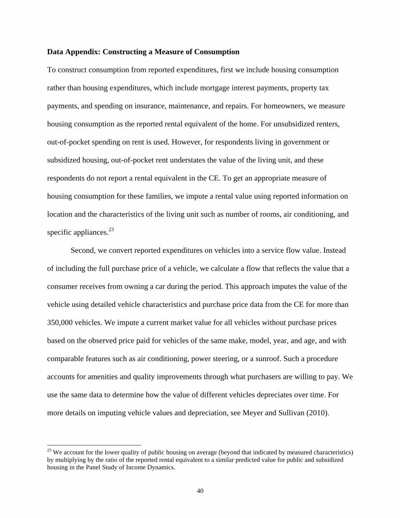
40

Data Appendix: Constructing a Measure of Consumption To construct consumption from reported expenditures, first we include housing consumption

rather than housing expenditures, which include mortgage interest payments, property tax

payments, and spending on insurance, maintenance, and repairs. For homeowners, we measure

housing consumption as the reported rental equivalent of the home. For unsubsidized renters,

out-of-pocket spending on rent is used. However, for respondents living in government or

subsidized housing, out-of-pocket rent understates the value of the living unit, and these

respondents do not report a rental equivalent in the CE. To get an appropriate measure of

housing consumption for these families, we impute a rental value using reported information on

location and the characteristics of the living unit such as number of rooms, air conditioning, and

specific appliances.23

Second, we convert reported expenditures on vehicles into a service flow value. Instead

of including the full purchase price of a vehicle, we calculate a flow that reflects the value that a

consumer receives from owning a car during the period. This approach imputes the value of the

vehicle using detailed vehicle characteristics and purchase price data from the CE for more than

350,000 vehicles. We impute a current market value for all vehicles without purchase prices

based on the observed price paid for vehicles of the same make, model, year, and age, and with

comparable features such as air conditioning, power steering, or a sunroof. Such a procedure

accounts for amenities and quality improvements through what purchasers are willing to pay. We

use the same data to determine how the value of different vehicles depreciates over time. For

more details on imputing vehicle values and depreciation, see Meyer and Sullivan (2010).

23 We account for the lower quality of public housing on average (beyond that indicated by measured characteristics) by multiplying by the ratio of the reported rental equivalent to a similar predicted value for public and subsidized housing in the Panel Study of Income Dynamics.

41

Third, we exclude from consumption out-of-pocket health expenses because these

expenses are not closely tied to well-being. For example, unhealthy individuals without full

insurance may have high out-of-pocket health expenses that do not reflect greater well-being. In

a measure that we use as a robustness check, we include an imputed value of health insurance.

We impute a value of private insurance for families that have private coverage, and a value of

Medicaid, Medicare, or Medigap coverage for families enrolled in these programs. These values

are determined using data on the average cost of such insurance by group. Data on the value of

private health insurance come from several sources, including the 1977 National Medical Care

Expenditure Survey and the Mercer/Foster Higgins National Survey of Employer-Sponsored

Health Plans. We distinguish between the value of individual and family plans. We use

administrative data on the cost of public health insurance to value Medicaid and Medicare. To

account for the fact that, for some families with few resources, the value of subsidized health

insurance exceeds the price they would be willing to pay, we limit the imputed value of health

insurance for each family so it does not exceed a predetermined share of total expenditures. We

do not report results for this measure that adds an imputed value of health insurance, but we have

verified that the patterns for the measure with this value are similar to those reported in this

paper.

Fourth, our consumption measure excludes spending that is better interpreted as an

investment, such as spending on education, and outlays for retirement, including pensions and

Social Security. We also exclude spending on charitable contributions, cash gifts to nonfamily

members, and other miscellaneous spending. This last category is excluded because it is not

collected for all observations. These excluded categories are very small relative to total

consumption.

42

Finally, we adjust this measure of total consumption to address concerns about

underreporting of consumption and changes in reporting rates in the CE for some components of

consumption over time. These concerns arise because comparisons of CE spending to Personal

Consumption Expenditure data from the National Income and Product Accounts suggest

substantial underreporting in the CE, and the underreporting has grown over time. To adjust for

changing underreporting, we estimate the relationship between total consumption and

components of consumption that tend to be reported well and demographic characteristics in

1980 and 1981.24 We choose these years because total expenditures in the CE compare more

favorably to national income account data in the early 1980s than in recent years. This estimated

relationship is then used to predict consumption for each family in all years.

Figure A1 reports the median and tenth percentile for our measure of consumption, as

well as our measure before adjusting for underreporting (unadjusted consumption). Comparing

our preferred measure of consumption to the unadjusted measure shows that adjusting for

underreporting results in greater growth in consumption at both the median and the tenth

percentile. After adjusting for underreporting, both the median and the tenth percentile rose in

real terms by 54 percent between 1980 and 2009. During this period, the median for unadjusted

consumption rose by 35 percent while the tenth percentile grew by 43 percent.

24 More specifically, we regress consumption (in constant dollars) on a cubic in core consumption (which is the sum of food at home, rent plus utilities, transportation, gasoline, the value of owner-occupied housing, rental assistance, and the value of owned vehicles), a cubic in the age of the head, education of the head dummies, family type dummies, and race dummies for consumer units in the CE from the first quarter of 1980 through the third quarter of 1981.

Differences

1981 1989 1999 20041 20091989-1981

1999-1989

2004 -1999

2009 -1999

Housing Characteristics (American Housing Survey)Number of people in household 3.786 3.525 3.389 - 3.461 -0.261 -0.136 - 0.072Number of rooms in unit 5.783 5.901 5.874 - 6.036 0.118 -0.027 - 0.162Number of rooms (adjusted for household size) 5.678 6.060 6.253 - 6.389 0.382 0.193 - 0.136Square footage of unit N/A 1,708 1,846 - 1,993 - 138 - 147Square footage (adjusted for household size) N/A 1,735 1,934 - 2,088 - 200 - 153Water leak from inside in last 6 months N/A 0.127 0.101 - 0.091 - -0.026 - -0.010Water leak from outside in last 6 months N/A 0.193 0.132 - 0.104 - -0.061 - -0.028Unit has central or room air conditioning 0.582 0.716 0.817 - 0.882 0.134 0.101 - 0.065Unit has central air conditioning 0.271 0.409 0.546 - 0.670 0.138 0.137 - 0.124Unit has a dishwasher N/A 0.531 0.608 - 0.698 - 0.077 - 0.090Unit has a clothes dryer N/A 0.794 0.824 - 0.881 - 0.030 - 0.057Unit has a clothes washer N/A 0.847 0.853 - 0.897 - 0.006 - 0.044

Automobile Characteristics (Consumer Expenditure Survey)Whether own a car 0.949 0.953 0.933 - 0.948 0.004 -0.020 - 0.015Whether own multiple cars 0.328 0.326 0.324 - 0.368 -0.002 -0.003 - 0.044Auto transmission 0.741 0.721 0.780 0.817 - -0.020 0.058 0.038 -Power breaks 0.564 0.751 0.884 0.911 - 0.187 0.133 0.028 -Air conditioning 0.473 0.626 0.786 0.835 - 0.154 0.160 0.048 -Power steering 0.664 0.742 0.882 0.921 - 0.078 0.140 0.039 -Sun roof N/A 0.050 0.086 0.101 - - 0.036 0.016 -Turbo charger N/A 0.009 0.019 0.012 - - 0.010 -0.007 -Four wheel drive N/A 0.038 0.092 0.133 - - 0.053 0.042 -

1

Table 1: Mean Housing and Vehicle Characteristics for Households in the Middle Twenty Percent of the Income Distribution, 1981-2009

2004 is the most recent year data are available for auto transmission, power breaks, air conditioning, power steering, sun roof, turbo charger, and four wheel drive.

Sources: Authors' calculations using the American Housing Survey and Consumer Expenditure Survey.Notes: The reported means are household size weighted and are for those in the middle quintile of the equivalence scale adjusted household income distribution. Forhouseholds with more than one vehicle, the characteristics of the car with the highest market value are reported.

Differences

1981 1989 1999 20041 20091989-1981

1999-1989

2004 -1999

2009 -1999

Housing Characteristics (American Housing Survey)Number of people in household 3.975 3.789 3.592 - 3.693 -0.186 -0.197 - 0.101Number of rooms in unit 5.126 5.133 5.157 - 5.283 0.007 0.024 - 0.126Number of rooms (adjusted for household size) 5.229 5.495 5.669 - 5.722 0.266 0.174 - 0.053Square footage of unit N/A 1,345 1,489 - 1,551 - 144 - 62Square footage (adjusted for household size) N/A 1,439 1,645 - 1,695 - 206 - 50Water leak from inside in last 6 months N/A 0.175 0.132 - 0.107 - -0.043 - -0.025Water leak from outside in last 6 months N/A 0.187 0.126 - 0.119 - -0.061 - -0.007Unit has central or room air conditioning 0.409 0.542 0.716 - 0.830 0.133 0.174 - 0.114Unit has central air conditioning 0.149 0.233 0.397 - 0.544 0.084 0.164 - 0.147Unit has a dishwasher N/A 0.222 0.311 - 0.422 - 0.089 - 0.111Unit has a clothes dryer N/A 0.481 0.567 - 0.679 - 0.086 - 0.112Unit has a clothes washer N/A 0.651 0.671 - 0.739 - 0.020 - 0.068

Automobile Characteristics (Consumer Expenditure Survey)Whether own a car 0.691 0.704 0.733 - 0.763 0.013 0.029 - 0.031Whether own multiple cars 0.208 0.211 0.223 - 0.222 0.003 0.011 - 0.000Auto transmission 0.769 0.766 0.823 0.858 - -0.003 0.057 0.035 -Power breaks 0.600 0.766 0.888 0.898 - 0.165 0.123 0.010 -Air conditioning 0.467 0.621 0.755 0.769 - 0.154 0.134 0.015 -Power steering 0.639 0.763 0.883 0.917 - 0.125 0.120 0.034 -Sun roof N/A 0.049 0.071 0.071 - - 0.022 0.000 -Turbo charger N/A 0.003 0.014 0.017 - - 0.011 0.002 -Four wheel drive N/A 0.040 0.081 0.081 - - 0.042 0.000 -

1

Table 2: Mean Housing and Vehicle Characteristics for Households in the Bottom Twenty Percent of the Income Distribution, 1981-2009

Sources: Authors' calculations using the American Housing Survey and Consumer Expenditure Survey.Notes: The reported means are household size weighted and are for those in the middle quintile of the equivalence scale adjusted household income distribution. Forhouseholds with more than one vehicle, the characteristics of the car with the highest market value are reported.

2004 is the most recent year data are available for auto transmission, power breaks, air conditioning, power steering, sun roof, turbo charger, and four wheel drive.

Change1980-2000

Change2000-2009

A. Consumption10th Percentile

Actual Change 23.3% 16.8%Change due to demographic characteristics 3.4% 0.5%

MedianActual Change 28.6% 15.2%Change due to demographic characteristics 3.3% 2.6%

B. After-tax Income Plus Noncash Benefits10th Percentile

Actual Change 31.4% 1.9%Change due to demographic characteristics 3.5% -3.6%

MedianActual Change 39.9% 7.2%Change due to demographic characteristics 3.0% 0.0%

Sources: Authors' calculations using the Consumer Expenditure Survey (consumption) and Current PopulationSurvey (income).Notes: The change due to demographic characteristics is calculated following the approach from Melly (2005) asexplained in the text. The characteristics used include family type, employment, race, and education. Changesare expressed in real terms using the adjusted CPI-U-RS.

Table 3: The Effect of Changes in Demographic Characteristics on Changes in Median and 10th Percentile of Income and Consumption, 1980-2009

1980 2000 2009Change

1980-2009A. Consumption Poverty

Actual Poverty 0.130 0.056 0.031 -0.099Predicted poverty holding within group poverty at 1980 rate

Changes in family type 0.130 0.141 0.142 0.012Changes in family type and employment 0.130 0.138 0.145 0.016Changes in family type and race 0.130 0.153 0.162 0.032Changes in family type, education, and employment 0.130 0.104 0.103 -0.027

B. After-tax Income Plus Noncash Benefits PovertyActual Poverty 0.130 0.063 0.067 -0.063Predicted poverty holding within group poverty at 1980 rate

Changes in family type 0.130 0.139 0.143 0.013Changes in family type and employment 0.130 0.137 0.155 0.025Changes in family type and race 0.130 0.148 0.158 0.028Changes in family type, education, and employment 0.130 0.115 0.124 -0.006

Sources: Authors' calculations using the Consumer Expenditure Survey (consumption) and Current Population Survey (income).Notes: Actual poverty rates are those reported in Figure 7. Predicted poverty is the weighted average of the poverty rates for each groupin 1980 using as weights the distribution across groups in the year listed in the column headings. All poverty rates are calculated usingthe adjusted CPI-U-RS.

Table 4: The Effect of Changes in Demographic Characteristics on Changes in Poverty, 1980-2009

$0

$5,000

$10,000

$15,000

$20,000

$25,000

$30,000

$35,000

$40,000

$45,000

5th 10th 20th 30th 40th 50th

(200

5 $)

Expenditures (CE Survey)

After-Tax Money Income Plus Food Stamps (CPS)

Figure 1: Percentiles of Income and Expenditures, All Families, CPS and CE Survey, 1993-2003

Source: Table 2 of Meyer and Sullivan (2011). Notes: These family level outcomes are expressed in real terms (2005 dollars) and adjusted for differences in family sizeusing the NAS recommended equivalence scale and normalized to a family with one adult and two children.

5th 10th 20th 30th 40th 50thPercentiles of Consumption or Income

15,000

20,000

25,000

30,000

35,000

40,000

45,000

50,000

55,000

60,000

65,000

Med

ian

(200

5 $)

Figure 2: Median Pre-tax Money Income, 1980-2009

Pre-tax Money Income--Official (CPI-U-RS)

Pre-tax Money Income (CPI-U-RS)

Pre-tax Money Income (Adjusted CPI-U-RS)

Source: Authors' calculations using the Current Population Survey.Notes: All measures are reported in 2005 dollars using either the CPI-U-RS or the adjusted CPI-U-RS. All measures other than the official measure, areadjusted for differences in family size using the NAS recommended equivalence scale. We multiply each scale adjusted measure by 2.14, the mean adultequivalent value across all years in the CE Survey from 1980-2005. The unit of observation for the official measure is the household, while it is the family for theother income measures. The Official measure is household weighted, while the other measures are person weighted.

0

5,000

10,000

15,000

1980

1981

1982

1983

1984

1985

1986

1987

1988

1989

1990

1991

1992

1993

1994

1995

1996

1997

1998

1999

2000

2001

2002

2003

2004

2005

2006

2007

2008

2009

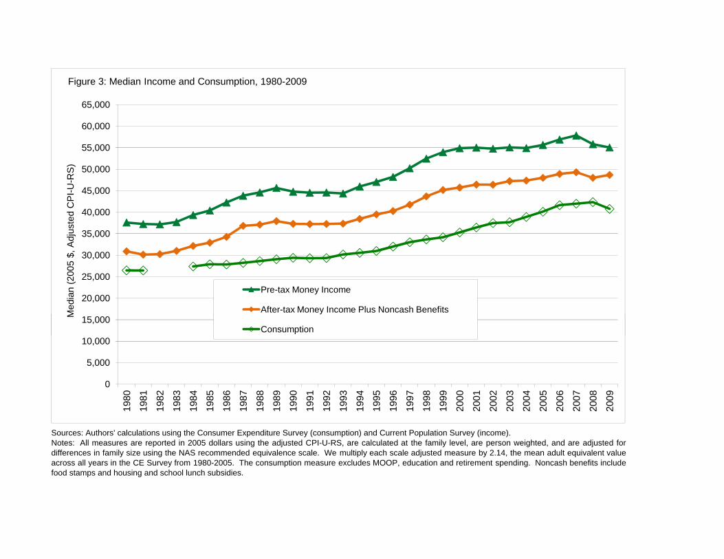
15,000

20,000

25,000

30,000

35,000

40,000

45,000

50,000

55,000

60,000

65,000

Med

ian

(200

5 $,

Adj

uste

d C

PI-U

-RS

)Figure 3: Median Income and Consumption, 1980-2009

Pre-tax Money Income

After-tax Money Income Plus Noncash Benefits

Consumption

Sources: Authors' calculations using the Consumer Expenditure Survey (consumption) and Current Population Survey (income).Notes: All measures are reported in 2005 dollars using the adjusted CPI-U-RS, are calculated at the family level, are person weighted, and are adjusted fordifferences in family size using the NAS recommended equivalence scale. We multiply each scale adjusted measure by 2.14, the mean adult equivalent valueacross all years in the CE Survey from 1980-2005. The consumption measure excludes MOOP, education and retirement spending. Noncash benefits includefood stamps and housing and school lunch subsidies.

0

5,000

10,000

15,000

1980

1981

1982

1983

1984

1985

1986

1987

1988

1989

1990

1991

1992

1993

1994

1995

1996

1997

1998

1999

2000

2001

2002

2003

2004

2005

2006

2007

2008

2009

M

Consumption

6 000

8,000

10,000

12,000

14,000

16,000

18,000

20,000

22,000

10th

Per

cent

ile (2

005

$)Figure 4: 10th Percentile of Income, 1980-2009

Pre-tax Money Income--Official (CPI-U-RS)

Pre-tax Money Income (CPI-U-RS)

Pre-tax Money Income (Adjusted CPI-U-RS)

Source: Authors' calculations using the Current Population Survey.Notes: See notes to Figure 2.

0

2,000

4,000

6,000

,

1980

1981

1982

1983

1984

1985

1986

1987

1988

1989

1990

1991

1992

1993

1994

1995

1996

1997

1998

1999

2000

2001

2002

2003

2004

2005

2006

2007

2008

2009

6 000

8,000

10,000

12,000

14,000

16,000

18,000

20,000

22,000

th P

erce

ntile

(200

5 $,

Adj

uste

d C

PI-U

-RS

)Figure 5: 10th Percentile of Income and Consumption, 1980-2009

Pre-tax Money Income

Sources: Authors' calculations using the Consumer Expenditure Survey (consumption) and Current Population Survey (income).Notes: See notes to Figure 3.

0

2,000

4,000

6,000

,

1980

1981

1982

1983

1984

1985

1986

1987

1988

1989

1990

1991

1992

1993

1994

1995

1996

1997

1998

1999

2000

2001

2002

2003

2004

2005

2006

2007

2008

2009

10th

Pe

Pre-tax Money Income

After-tax Money Income Plus Noncash Benefits

Consumption

0.04

0.05

0.06

0.07

0.08

0.09

0.1

0.11

0.12

0.13

0.14

0.15

0.16

Frac

tion

Poo

r

Pre-tax Money Income--Offical (CPI-U)

Pre-tax Money Income (NAS Scale, CPI-U-RS)

Pre-tax Money Income (NAS Scale, Adjusted CPI-U-RS)

Figure 6: Income Poverty Rates, 1980-2009

Source: Authors' calculations using the Current Population Survey.Notes: The rates are anchored at the official rate in 1980. Poverty status is determined at the family level and then person weighted.

0.02

0.03

0.04

1980

1981

1982

1983

1984

1985

1986

1987

1988

1989

1990

1991

1992

1993

1994

1995

1996

1997

1998

1999

2000

2001

2002

2003

2004

2005

2006

2007

2008

2009

Pre-tax Money Income (NAS Scale, Adjusted CPI-U-RS)

0.04

0.05

0.06

0.07

0.08

0.09

0.10

0.11

0.12

0.13

0.14

0.15

0.16

Frac

tion

Poo

r

Pre-tax Money Income (NAS Scale, Adjusted CPI-U-RS)

After-tax Money Income Plus Noncash Benefits (NAS Scale, Adjusted CPI-U-RS)

Consumption (NAS Scale, Adjusted CPI-U-RS)

Figure 7: Consumption and Income Poverty Rates, 1980-2009

Sources: Consumer Expenditure Survey (consumption) and Current Population Survey (income).Notes: The rates are anchored at the official rate in 1980. Poverty status is determined at the family level and then person weighted. Consumption data are not available forthe years 1982-1983. The consumption measures excludes MOOP, education and retirement spending. Noncash benefits include food stamps and housing and schoollunch subsidies.

0.02

0.03

0.04

1980

1981

1982

1983

1984

1985

1986

1987

1988

1989

1990

1991

1992

1993

1994

1995

1996

1997

1998

1999

2000

2001

2002

2003

2004

2005

2006

2007

2008

2009

15,000

20,000

25,000

30,000

35,000

40,000

45,000

50,000

55,000

60,000

65,000

Med

ian

(200

5 $)

Figure 8a: Median Pre-tax Money Income with and without Transfers and Pre-tax and After-tax Earnings, 1980-2009

Pre-tax Money Income (Adjusted CPI-U-RS)

Pre-tax, Pre-transfer Money Income (Adjusted CPI-U-RS)

Pre-tax Earnings (Adjusted CPI-U-RS)

Source: Authors' calculations using the Current Population Survey.Notes: Both measures are reported in 2005 dollars using the adjusted CPI-U-RS, are calculated at the family level, are person weighted, and are adjusted fordifferences in family size using the NAS recommended equivalence scale. We multiply each scale adjusted measure by 2.14, the mean adult equivalent valueacross all years in the CE Survey from 1980-2005. The government transfers excluded from the pre-transfer measure of income include social security,unemployment insurance, workers' compensation, veterans benefits, SSI, and AFDC/TANF.

0

5,000

10,000

15,000

1980

1981

1982

1983

1984

1985

1986

1987

1988

1989

1990

1991

1992

1993

1994

1995

1996

1997

1998

1999

2000

2001

2002

2003

2004

2005

2006

2007

2008

2009

Pre-tax Earnings (Adjusted CPI-U-RS)

6 000

8,000

10,000

12,000

14,000

16,000

18,000

20,000

22,000

10th

Per

cent

ile (2

005

$)Figure 8b: 10th Percentile of Income, 1980-2009

Pre-tax Money Income (Adjusted CPI-U-RS)

Pre-tax, Pre-transfer Money Income (Adjusted CPI-U-RS)

Source: Authors' calculations using the Current Population Survey.Notes: See notes to Figures 2a and 2b.

0

2,000

4,000

6,000

,

1980

1981

1982

1983

1984

1985

1986

1987

1988

1989

1990

1991

1992

1993

1994

1995

1996

1997

1998

1999

2000

2001

2002

2003

2004

2005

2006

2007

2008

2009

0.04

0.05

0.06

0.07

0.08

0.09

0.1

0.11

0.12

0.13

0.14

0.15

0.16

Frac

tion

Poo

r

Pre-tax Money Income (NAS Scale, Adjusted CPI-U-RS)

Pre-tax, Pre-transfer Money Income (NAS Scale, Adjusted CPI-U-RS)

Figure 8c: Income Poverty Rates, 1980-2009

Source: Authors' calculations using the Current Population Survey.Notes: The rates are anchored at the official rate in 1980. Poverty status is determined at the family level and then person weighted. The government transfers excludedfrom the pre-transfer measure of income include social security, unemployment insurance, workers' compensation, veterans benefits, SSI, and AFDC/TANF.

0.02

0.03

0.04

1980

1981

1982

1983

1984

1985

1986

1987

1988

1989

1990

1991

1992

1993

1994

1995

1996

1997

1998

1999

2000

2001

2002

2003

2004

2005

2006

2007

2008

2009

15,000

20,000

25,000

30,000

35,000

40,000

45,000

(200

5 $,

Adj

uste

d C

PI-U

-RS)

Appendix Figure 1: Median and 10th Percentile of Consumption with and without Adjusting for Under-reporting, 1980-2009

Sources: Authors' calculations using the Consumer Expenditure Survey.Notes: All measures are reported in 2005 dollars using the adjusted CPI-U-RS. See Figure 5 for additional notes.

0

5,000

10,000

15,000

1980

1981

1982

1983

1984

1985

1986

1987

1988

1989

1990

1991

1992

1993

1994

1995

1996

1997

1998

1999

2000

2001

2002

2003

2004

2005

2006

2007

2008

2009

Median Consumption

Median Consumption (unadjusted)

10th Percentile Consumption

10th Percentile Consumption (unadjusted)