Mon. Not. R. Astron. Soc. 000, 000–000 (0000) Printed 5 October 2016 (MN LATEX style file v2.2)

The Mass Function of Unprocessed Dark Matter Halos andMerger Tree Branching Rates

Andrew J. Benson11 Carnegie Observatories, 813 Santa Barbara Street, Pasadena, CA 91101, USA.

5 October 2016

ABSTRACTA common approach in semi-analytic modeling of galaxy formation is to constructMonte Carlo realizations of merger histories of dark matter halos whose masses aresampled from a halo mass function. Both the mass function itself, and the merger ratesused to construct merging histories are calibrated to N-body simulations. Typically,“backsplash” halos (those which were once subhalos within a larger halo, but whichhave since moved outside of the halo) are counted in both the halo mass function,and in the merger rates (or, equivalently, progenitor mass functions). This leads toa double-counting of mass in Monte Carlo merger histories which will bias resultsrelative to N-body results. We measure halo mass functions and merger rates withthis double-counting removed in a large, cosmological N-body simulation with cosmo-logical parameters consistent with current constraints. Furthermore, we account forthe inherently noisy nature of N-body halo mass estimates when fitting functions toN-body data, and show that ignoring these errors leads to a significant systematicbias given the precision statistics available from state-of-the-art N-body cosmologicalsimulations.

Key words: cosmology: theory, dark matter

1 INTRODUCTION

In the cold dark matter (CDM) cosmogony, structure formsthrough the hierarchical merging of dark matter halos (Daviset al. 1985). The distribution of halo masses at a given epochin the universe is a topic of significant interest and has beenstudied extensively (Press & Schechter 1974; Bond et al.1991; Jenkins et al. 2001; Sheth & Tormen 2002; White 2002;Luki et al. 2007; Reed et al. 2003; Warren et al. 2006; Reedet al. 2007; Tinker et al. 2008). The standard definition of ahalo is a region of dark matter which has undergone gravi-tational collapse and which exists in a state at least close tovirial equilibrium. Practically, halos are typically defined asregions around density peaks whose mean density exceedssome threshold value, often motivated by the simple spher-ical top-hat collapse model (e.g. Press & Schechter 1974).Recently, Despali et al. (2015) have shown that this choiceof density threshold should be preferred as it results in themost universal mass function when expressed in terms ofthe rescaled mass variable1, ν = δc/σ(M), where δc is the

1 While this is good motivation for choosing a particular defini-tion of halo (it is at least motivated by a simple physical model

and, as Despali et al. (2015) show, leads to the most universal

mass function), it is highly idealized, and there is no notable phys-ical distinction to this radius. It may be more robust therefore to

critical linear theory overdensity for a halo to undergo grav-itational collapse, and σ(M) is the amplitude of fluctuationsin spheres containing, on average, mass M in the linear den-sity field at the present day.

Since halos grow hierarchically it was long suspectedthat the remnants of earlier generations of halos would sur-vive for some time inside the larger halos into which theymerge. This was confirmed by Moore et al. (1999) andKlypin et al. (1999), and is now a well-established fact inthe CDM paradigm. Since many of these subhalos can sur-vive for many dynamical times, and initially cross the virialradius of the halo with non-zero radial velocity, it should notbe surprising that some subhalos are able to exit the virialradius once again as their orbit carries them toward apoc-entre2. These “backsplash” halos have also been identifiedin N-body simulations (Moore et al. 2004; Gill et al. 2005;

characterize dark matter halos by some other quantity, such as the

peak velocity in their rotation curve, and construct a Vmax func-

tion instead. Better still, halos could be characterized by a twoparameter function, specifying their abundance as a function of

Vmax and rs (the scale radius in the Navarro et al. (1997) density

profile). Together those two parameters specify the complete den-sity profile of a halo, allowing its mass under any definition to be

easily computed, and does not rely on a specific mass definition.

We address this issue further in Benson (2017, in preparation).2 Some halos will not exit the halo of course, due to the effects of

c© 0000 RAS

arX

iv:1

610.

0105

7v1

[as

tro-

ph.G

A]

4 O

ct 2

016

2 Andrew J. Benson

Warnick et al. 2008; Ludlow et al. 2009) with around 30%of subhalos with orbital pericentres lying within the virialradius being found outside the virial radius at z = 0 (Gillet al. 2005). The backsplash population may differ signifi-cantly in its properties due to the environmental effects ofthe host halos through which they have passed (Knebe et al.2011). It could be argued, therefore, that these backsplashhalos should be excluded from measurements of the massfunction and treated as a separate population.

Furthermore, in studies which employ merger treesgenerated using the extended Press-Schechter methodology(Lacey & Cole 1993; or derivatives thereof, e.g. Parkinsonet al. 2008) to follow the hierarchical growth of structurethese backsplash halos can be double counted. The branch-ing rates used to construct merger trees are typically cal-ibrated to reproduce the conditional mass functions (thatis, the distribution of progenitor halo masses at some ear-lier time, conditioned on those progenitors being part of ahalo of given mass at some given later time). These condi-tional mass functions will inevitably (and correctly) includesome halos which later become backsplash halos. The prob-lem arises when ensembles of merger trees are averaged over(e.g. to construct galaxy mass functions). Here, the weightassigned to each merger tree is proportional to the halo massfunction in order to give a fair sampling. But, under stan-dard definitions, the halo mass function will include thosesame backsplash halos which were already included in con-ditional mass functions to which the merger tree branchingrates were calibrated. As a result, the population of back-splash halos is double counted. This will bias estimates ofany quantity computed by averaging over an ensemble ofmerger trees constructed in this way, and will manifest itselfwhenever comparing results based on merger trees extractedfrom N-body simulations, and those based on trees built us-ing extended Press-Schechter-based approaches to mimic theN-body trees.

In this work, we construct and examine halo mass func-tions from which backsplash halos have been excluded. Weprovide a calibration of the fitting function of Sheth & Tor-men (2002) which approximately reproduces these “back-splashless” mass functions and which can therefore be usedin computing unbiased averages over ensembles of mergertrees. Additionally, we provide a recalibration of merger treebranching rates using the fitting function of PCH, for up-dated cosmological parameters, with a significantly largercalibration set and defined consistently with our halo massfunction (i.e. with z = 0 backsplash halos excluded3).

The remainder of this paper is organized as follows. In§2 we describe the N-body data employed as our calibra-tion dataset, the construction of halo mass functions andconditional mass functions, and our treatment of the errorsin N-body halo mass estimates. We present the results of

dynamical friction, the time evolution of the host halo potential,

and possible tidal destruction.3 Standard extended Press-Schechter-type approaches do notprovide spatial information on subhalos, and so cannot make pre-dictions about the population of backsplash halos. Such predic-tions could plausibly be made however if the technique was aug-

mented through the inclusion of a dynamical model for subhalo

orbits (Taylor & Babul 2001; Benson et al. 2002; Zentner et al.2005).

our calibrations in §3, and discuss their implications in §4.Finally, in §5 we give our conclusions.

2 METHOD

In this section we describe how we measure mass func-tions from the MultiDark Planck N-body (MDPL) simula-tion (Klypin et al. 2016), and how we construct model massfunctions and conditional mass functions. We make exten-sive use of the analysis facilities of the Galacticus galaxyformation toolkit (Benson 2012) to perform these tasks.

2.1 N-body Data

For this work we utilize the MDPL simulation (Klypinet al. 2016). This simulation has a box size of 1.48 Gpc,contains 38403 particles each of mass 1.70 × 109M,and adopts cosmological parameters consistent with mea-surements from the Planck satellite (Planck Collabo-ration et al. 2014), namely (H0,ΩΛ,ΩM,Ωb, n, σ8) =(67.77 km/s/Mpc, 0.6929, 0.3071, 0.04820, 0.96, 0.8228). Ha-los were identified using the RockStar algorithm (Behrooziet al. 2013a), and merger trees were constructed from thesehalos using the ConsistentTrees algorithm (Behrooziet al. 2013b). RockStar provides several masses for eachhalo—in this work we exclusively make use of the “virialmass” supplied by RockStar which is defined as the masswithin a sphere of mean density given by the fitting formulaof Bryan & Norman (1998) to spherical top-hat collapse so-lutions (and is therefore consistent with the preferred massof Despali et al. 2015). The resulting merger trees contain88 time snapshots between z = 0 and z = 9.34.

2.2 Halo Mass Functions

The standard mass function can be found from an N-body simulation by counting halos into bins logarithmicallyspaced in halo mass. For the backsplashless mass function wemust first identify, and then exclude, all backsplash halos—that is, any halo which was identified as a subhalo in anyprevious timestep. As we have merger trees this is a straight-forward exercise. Galacticus computes for each halo in amerger tree both the current and highest-ever “hierarchylevel”. Hierarchy level is defined to be 0 for an isolated halo(i.e. a halo which is not contained within any other halo),andN+1 for a halo contained within a halo of hierarchy levelN . Thus, level-1 halos are subhalos, level-2 are sub-subhalos,etc. A backsplash halo has a current hierarchy level of 0, anda maximum hierarchy level ever reached greater than 0.

We find that, while this definition of backsplash haloshas the virtue of being simple, it leads to implausible be-haviour. In particular, many very high mass halos are iden-tified as backsplash halos. This happens because, very earlyin the history of the halo, its primary progenitor (at thetime of low mass) can be identified as a subhalo—this isthen recorded in the maximum hierarchy level reached allthe way to the final halo. This subhalo identification is likelyspurious and reflects the difficulties of assigning which is theprimary halo (Srisawat et al. 2013).

Therefore, we reset the maximum hierarchy level to zeroif a halo is currently level 0 and its current mass exceeds its

c© 0000 RAS, MNRAS 000, 000–000

3

mass when it was last a subhalo by a factor freset—thatis, if Mcurrent > fresetMsub. We would typically not expectbacksplash halos to grow significantly in mass, as they (bydefinition) do not dominate their local potential. We choosefreset = 2 as our canonical value. Our results are somewhatsensitive to this choice. At the lowest halo masses studied inthis work (corresponding to 300 particles), we find that back-splash halos make up 7% of all halos for freset = 2. Increas-ing freset to 4 increases this fraction to 9%, while decreasingfreset to 1 (which is not recomended as any upward fluctua-tion in halo mass would then trigger the maximum hierarchylevel to be reset to zero, but is included here as an extremecase) results in a 4% backsplash fraction (for 3000 particlehalos these fractions become 1.09%, 1.43%, and 0.36% re-spectively, so that even at higher particle number the choiceof freset still makes a significant difference in the fraction ofbacksplash halos, although that fraction is smaller overall).Improvement in this aspect of backsplash halo identificationwill require the development of more robust algorithms formerger tree construction and the assignment of primary halostatus.

To model the resulting backsplashless mass functionwe use the parametric form proposed by Sheth & Tormen(2002),

dn

dM(M) =

AΩMρc

M2

∣∣∣∣ d log σ

d logM(M)

∣∣∣∣ ( 2

πν′)1/2(

1 +1

ν′p

)× exp

(−1

2ν′), (1)

with ν′ = aν2, but convolved with the N-body halo masserror distribution described in §2.4, allowing the three pa-rameters a, p, and A (the overall normalization) to vary.This parametric form was also used by Despali et al. (2015).To find the optimal values of the parameters (a, p, A) weperform a Markov Chain Monte Carlo (MCMC) simulationin which these parameters are allowed to vary.

2.3 Merger Tree Branching Rates

To constrain the branching rates in merger trees we firstconstruct conditional halo mass functions from the MDPLsimulation. In particular, we measure from the MDPL thedistribution of progenitor halo masses at several redshiftsz > 0 of halos selected in mass bins at z = 0. We thenuse the algorithm of Parkinson et al. (2008; hereafter PCH)to construct merger trees spanning the same range of halomass and redshift. These merger trees are built with a massresolution of Mres = 6.684 × 1010M, corresponding to 40particles in the MDPL simulation, and well below the limit-ing mass (corresponding to 300 particles) which we will usein our analyses. Timesteps in the PCH branching algorithmare chosen to be sufficiently small that the probability ofmultiple branching is less than 1%, the fraction of mass ac-creted in the form of unresolved halos is less than 1%, andthat the first order approximation made in equation (2) ofPCH is always valid.

To compute branching rates in merger trees, the PCHalgorithm utilizes the progenitor mass function in the limitof infinitesimal timesteps as predicted by extended Press-Schechter theory (Lacey & Cole 1993), multiplied by a cor-

rective factor

G(σ1, σ2, δ2) = G0

(σ1

σ2

)γ1 ( δ2σ2

)γ2, (2)

where σi = σ(Mi), with i = 1 corresponding to the progen-itor halo, and i = 2 the parent halo, while δ2 is the criticaloverdensity for collapse at the time of the parent halo.

To find the optimal values of the parameters (G0, γ1, γ2)we perform an MCMC simulation in which these parametersare allowed to vary.

2.4 Errors in N-body Halo Masses

Dark matter halos in N-body simulations consist of a num-ber of particles, which represent a random sampling of theunderlying dark matter distribution function in the halo.This finite particle representation will inevitably lead to er-rors in measured properties of the halos. In this work we areconcerned with halo masses. To estimate the uncertaintiesin halo masses arising from finite numbers of particles weperform a simple experiment. Namely we simulate a largenumber of spherical, isothermal (i.e. with density profilesρ ∝ r−2) dark matter halos represented with different num-bers of particles. We then apply friends-of-friends (Daviset al. 1985; FoF) and spherical overdensity (Lacey & Cole1994; SO) halo finder algorithms to determine the mass ofeach realization. From these results we find both the meanand scatter in the recovered halo mass as a function of thenumber of particles used. Figure 1 shows the results for bothhalo finder algorithms. As is well known (and which can bepredicted from percolation theory and is shown by the solidblue line in the left panel of Figure 1; More et al. 2011) theFoF algorithm returns halo masses biased high at low num-bers of particles. The SO algorithm does not (at least in thissimple case, by construction). We find both algorithms showsignificant random errors in recovered halo masses. In thecase of the FoF algorithm, we find that the standard devia-tion of these random errors can be described by the simplerelation σ(N) ≈ 1.2N−1/2, where N is the mean number ofparticles in the halo.

In the case of the SO algorithm, the standard deviationof the random errors on halo mass can be derived analyt-ically. Consider a sphere of fixed radius, corresponding tothe radius of a halo (as defined by the SO algorithm densitythreshold in the limit of an infinitely well-resolved halo),centred on the location of that halo. We expect the num-ber of particles within this sphere to be a random variable,drawn from a Poisson distribution with mean 〈N〉 = M/mp,where M is the true mass of the halo, and mp is the particlemass of the simulation. If the number of particles inside thesphere fluctuates high the density is increased and the SOalgorithm must grow the radius larger to reach its specifieddensity threshold. The mass within the SO sphere is there-fore raised even further. The opposite happens if N fluctu-ates low. The variance in halo mass is therefore expected tobe larger than that of a Poisson distribution with mean 〈N〉.Specifically, if we consider the change in the radius of thehalo necessary to return to the same mean enclosed densitywhen the mass inside the original sphere fluctuates by δMwe find that the additional mass gained by this fluctuation

c© 0000 RAS, MNRAS 000, 000–000

4 Andrew J. Benson

0.9

1

1.1

1.2

1.3

1.4

1.5

102 103 104

Rec

over

edno

rmal

ized

mas

s;M

FoF/M∞

Particle number; N

Errors in FoF Halo Mass EstimatesErrors in FoF Halo Mass Estimates

0.6

0.7

0.8

0.9

1

1.1

1.2

1.3

1.4

102 103 104

Rec

over

edno

rmal

ized

mas

s;M

SO

Particle number; N

Errors in SO Halo Mass EstimatesErrors in SO Halo Mass Estimates

Figure 1. The mass of N-body realizations of an idealized dark matter halo as recovered by FoF (left) and SO (right) halo finder

algorithms, as a function of the number of particles (on average) in the halo. Masses are normalized to the mass that would be obtainedin the limit of an infinite number of particles. Points indicate the mean mass found from a large number of halo realizations, with

errorbars indicating the standard deviation in mass over this sample. The blue solid line (shown only for the FoF case) indicates the

expectation for the mass based on a percolation theory analysis (More et al. 2011). Dotted blue lines indicate models for the standarddeviation in halo mass, as described in the text.

in radius is (to first order in δM):

δ′M = δM

[ρSO

ρs− 1

]−1

, (3)

where ρSO is the density threshold in the SO algorithm, andρs is the density at the surface of the unperturbed sphere.

If δM has root-variance σ we can find the root-varianceof δM ′, σ′, from the above. These two contributions tothe total root variance in M can be added linearly (not inquadrature as is usual with root-variances because, in thismodel, the two contributions are perfectly correlated). Thetotal fractional root-variance in M is then

σtotal = σ

1 +

[ρSO

ρs− 1

]−1. (4)

For an isothermal halo (ρSO/ρs = 3), and for our idealizedsimulation the variance is that of a binomial distributionwith p = 1/2, namely σ = 1/

√2N . The resulting root-

variance, σtotal is shown by the blue dotted line in Figure 1and agrees extremely well with the root-variance measureddirectly from our idealized simulations.

To test how well this error model performs on actualN-body simulations we extract a sample of several thousanddark matter halos from the Millennium simulation (Springelet al. 2005), identified using the friends-of-friends algorithm,and spanning a wide range of masses (corresponding to par-ticle numbers of around 102 to 105). For each halo, we ex-tract all particles within a cubic region of length 6 Mpc/h(sufficient to more than capture the entirety of the halo plusa significant region around it) centred at the halo centreof mass. We then resample the N particles in this region,with replacement, to produce a new sample of N particlesand compute the mass of the resampled halo using the SOalgorithm—a similar bootstrapping approach has recentlybeen used by Poveda-Ruiz et al. (2016) to study the er-rors and biases in N-body determinations of halo concentra-tions. This process is repeated 1000 times for each halo,

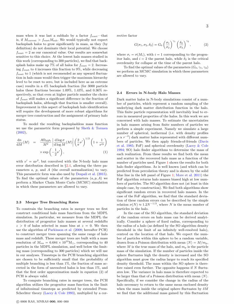
and the mean number of particles, and variance in thatnumber is computed from these realizations. Figure 2 showsthe resulting error on particle number for each halo (smallblack points), together with the mean error as a functionof the number of particles contained in the halo (adaptivelybinned such that each point corresponds to 400 halos; yellowpoints). Note that the particle number plotted is the meannumber found by the SO algorithm—in some instances thiscan be lower than the corresponding friends-of-friends halomass and so some points extend below N = 100. The blueline indicates Poisson (i.e.

√N) errors, while the green line

indicates errors predicted by equation (4) assuming Navarroet al. (1997) profiles with a Gao et al. (2008) concentration-mass relation to compute the ρSO/ρs term, and assumingσ = 1/

√N as appropriate if the number of particles within

the true halo radius (i.e. that which would be obtained inthe limit of an infinite number of particles) is Poisson dis-tributed.

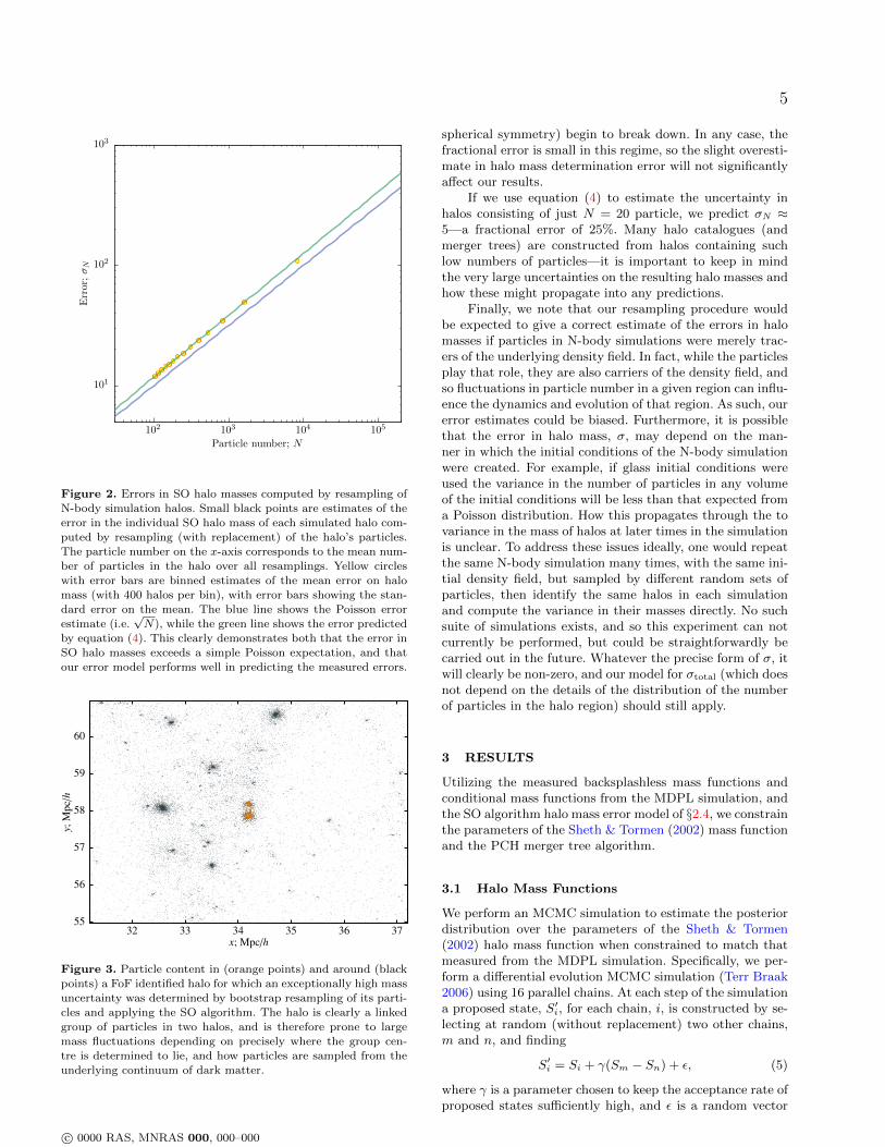
It is clear that the Poisson model (blue line) underpre-dicts the measured errors in halo mass, while the model spec-ified by equation (4) performs much better at predicting themeasured errors. We note that some of the individual haloerrors (shown as small black points) deviate substantiallyfrom the predicted line—this deviation is biased to highererrors. We find that in these cases the halo being resampledhas significant substructure nearby, or in some cases is alinked pair of halos (from the FoF algorithm) as shown inFig. 3, leading to much larger variations in the mass identi-fied by the SO algorithm as it was resampled than predictedby our model (which assumes a spherical halo with a smoothdensity profile). Despite these outliers it is clear that ourmodel performs well in predicting the error in the vast ma-jority of cases. It is also apparent that at the highest masses(i.e. highest particle numbers) our model prediction slightlyoverestimates the error in halo mass. This may be becausethe concentration–mass relation we employ is inaccurate inthis regime, or because the assumptions of our model (e.g.

c© 0000 RAS, MNRAS 000, 000–000

5

101

102

103

102 103 104 105

Error;σN

Particle number; N

Figure 2. Errors in SO halo masses computed by resampling of

N-body simulation halos. Small black points are estimates of theerror in the individual SO halo mass of each simulated halo com-

puted by resampling (with replacement) of the halo’s particles.

The particle number on the x-axis corresponds to the mean num-ber of particles in the halo over all resamplings. Yellow circles

with error bars are binned estimates of the mean error on halomass (with 400 halos per bin), with error bars showing the stan-

dard error on the mean. The blue line shows the Poisson error

estimate (i.e.√N), while the green line shows the error predicted

by equation (4). This clearly demonstrates both that the error in

SO halo masses exceeds a simple Poisson expectation, and that

our error model performs well in predicting the measured errors.

55

56

57

58

59

60

32 33 34 35 36 37

y;M

pc/h

x; Mpc/h

Figure 3. Particle content in (orange points) and around (blackpoints) a FoF identified halo for which an exceptionally high massuncertainty was determined by bootstrap resampling of its parti-cles and applying the SO algorithm. The halo is clearly a linked

group of particles in two halos, and is therefore prone to largemass fluctuations depending on precisely where the group cen-tre is determined to lie, and how particles are sampled from the

underlying continuum of dark matter.

spherical symmetry) begin to break down. In any case, thefractional error is small in this regime, so the slight overesti-mate in halo mass determination error will not significantlyaffect our results.

If we use equation (4) to estimate the uncertainty inhalos consisting of just N = 20 particle, we predict σN ≈5—a fractional error of 25%. Many halo catalogues (andmerger trees) are constructed from halos containing suchlow numbers of particles—it is important to keep in mindthe very large uncertainties on the resulting halo masses andhow these might propagate into any predictions.

Finally, we note that our resampling procedure wouldbe expected to give a correct estimate of the errors in halomasses if particles in N-body simulations were merely trac-ers of the underlying density field. In fact, while the particlesplay that role, they are also carriers of the density field, andso fluctuations in particle number in a given region can influ-ence the dynamics and evolution of that region. As such, ourerror estimates could be biased. Furthermore, it is possiblethat the error in halo mass, σ, may depend on the man-ner in which the initial conditions of the N-body simulationwere created. For example, if glass initial conditions wereused the variance in the number of particles in any volumeof the initial conditions will be less than that expected froma Poisson distribution. How this propagates through the tovariance in the mass of halos at later times in the simulationis unclear. To address these issues ideally, one would repeatthe same N-body simulation many times, with the same ini-tial density field, but sampled by different random sets ofparticles, then identify the same halos in each simulationand compute the variance in their masses directly. No suchsuite of simulations exists, and so this experiment can notcurrently be performed, but could be straightforwardly becarried out in the future. Whatever the precise form of σ, itwill clearly be non-zero, and our model for σtotal (which doesnot depend on the details of the distribution of the numberof particles in the halo region) should still apply.

3 RESULTS

Utilizing the measured backsplashless mass functions andconditional mass functions from the MDPL simulation, andthe SO algorithm halo mass error model of §2.4, we constrainthe parameters of the Sheth & Tormen (2002) mass functionand the PCH merger tree algorithm.

3.1 Halo Mass Functions

We perform an MCMC simulation to estimate the posteriordistribution over the parameters of the Sheth & Tormen(2002) halo mass function when constrained to match thatmeasured from the MDPL simulation. Specifically, we per-form a differential evolution MCMC simulation (Terr Braak2006) using 16 parallel chains. At each step of the simulationa proposed state, S′i, for each chain, i, is constructed by se-lecting at random (without replacement) two other chains,m and n, and finding

S′i = Si + γ(Sm − Sn) + ε, (5)

where γ is a parameter chosen to keep the acceptance rate ofproposed states sufficiently high, and ε is a random vector

c© 0000 RAS, MNRAS 000, 000–000

6 Andrew J. Benson

each component of which is drawn from a Cauchy distri-bution with median zero and width parameter set equal to10−3 of the current range of parameter values spanned bythe ensemble of chains to ensure that the chains are posi-tively recurrent. For a multivariate normal likelihood func-tion in N dimensions the optimal value of γ is γ0 = 2.38/

√N

(Terr Braak 2006). We use this as our initial value of γ, butadjust γ adaptively as the simulation progresses to maintaina reasonable acceptance rate. The proposed state is acceptedwith probability P where

P =

1 if L(S′i) > L(Si),L(S′i)/L(Si) otherwise,

(6)

and where L is the likelihood function.The simulation is allowed to progress until the chains

have converged on the posterior distribution as judged bythe Gelman-Rubin statistic, R (Gelman & Rubin 1992),after outlier chains (identified using the Grubb’s outliertest (Grubbs 1969; Stefansky 1972) with significance levelα = 0.05) have been discarded. Specifically, we declare con-vergence when R = 1.2.

The Gelman-Rubin convergence measure relies on thechains be initialized in an over dispersed state. The state ofeach chain is therefore initialized by constructing 16-pointunit Latin hypercubes. We generate 100 such cubes and findthe cube which maximizes the minimum (`2-norm) distancebetween any two points in the hypercube. Each point inthis hypercube realization is used as the initial state for achain by associating Ci = Li where Li is the ith coordinateof the point in the hypercube, and Ci is the cumulativeprobability distribution of the prior on parameter i. Theparameter values are then simply found by inverting theircumulative distributions. We choose broad, uninformativepriors for the parameters which span the range of valuesfound by previous studies, specifically, a = [0.05, 1.50], p =[−1,+1], A = [0.05, 1.00].

Our likelihood function is defined as

logL = −1

2

∑i

(φ

(model)i − φ(N-body)

i

)2

V(N-body)i

, (7)

where φ(model) is the mass function resulting from the Sheth& Tormen (2002) fitting function after convolution with thehalo mass error distribution, φ(N-body) is that measured inthe MDPL, V (N-body) is the variance in the N-body massfunctions (computed under the assumption that the num-ber of halos in each bin obeys Poisson statistics), subscripti runs over all bins in the mass functions above our im-posed resolution limit corresponding to 300 particles, andwhich contain at least 30 halos in the MDPL simulation. Incomputing the model expectation we average the convolvedSheth & Tormen (2002) mass function across the width ofeach bin used in estimating the MDPL mass function. Thisensures that any variation in the mass function across thebin is correctly accounted for.

We find that our MCMC chains converge after approx-imately 100 steps. We allow the simulation to run for ap-proximately 10,000 further steps, and measure a correlationlength in each parameter of around 10 steps, leaving us withapproximately 16,000 independent samples from the poste-rior distribution over the parameters.

Figure 4 shows mass functions at z = 0 and z ≈ 1

0.82 0.83 0.84 0.85 0.86 0.87 0.88 0.89 0.9a

−0.06

−0.04

−0.02

0

0.02

0.04

p

Figure 5. Constraints on mass function parameters, a and p. The

colour shading and purple contours show results for z = 0.0 withbacksplash halos excluded and with the mass function convolved

with the expected distribution of N-body halo mass errors. The

grey contours indicate constraints obtained ignoring errors in halomasses clearly demonstrating a significant offset.

measured from the MDPL simulation with and without theinclusion of backsplash halos (points), with the best fittingSheth & Tormen (2002) mass function (after convolutionby the error model of §2.4) indicated by lines. For refer-ence we also plot the mass function found by Despali et al.(2015). Table 1 lists the parameters of the best fit Sheth& Tormen (2002) mass function at z = 0, for cases wherebacksplash halos are included and excluded (along with re-sults for other redshifts, and for cases where the N-bodyhalo mass error distribution is not accounted for). For thecase with backsplash halos included the best fit parameterswe find are close to, but significantly different from, thosefound by Despali et al. (2015).

When backsplash halos are excluded the mass functionis changed significantly at low masses. This effect is morepronounced at z = 0 than at z = 1. At z = 0, the massfunctions with and without backsplash halos begin to devi-ate below 1013M, corresponding closely with the value ofM∗ (the characteristic halo mass defined by σ(M) = δc) atz = 0. This is to be expected: higher mass halos are stillin the stage dominated by growth via merging with smallersystems (and so are unlikely to have previously merged withany larger halo), while the evolution of lower mass halos isdominated by their merging into larger halos (e.g. Bensonet al. 2005).

The importance of convolving the fitting function withthe expected N-body halo mass error distribution is illus-trated in Figure 5 where we show the constraints on the pa-rameters a and p derived from our MCMC simulation. Thecolour shading and purple contours indicate the posteriordistribution over these parameters when fitting a convolvedmass function to the N-body data, while the grey contoursindicate the posterior distribution obtained if errors on N-body halo masses are ignored. Clearly, at the level of preci-sion that can be obtained from state-of-the-art N-body sim-ulations the treatment of errors has a very significant (muchgreater than 3σ) effect on the resulting parameters of fittingfunctions.

We use posterior predictive checks (PPCs) (Gilks 1995;

c© 0000 RAS, MNRAS 000, 000–000

7

10−10

10−8

10−6

10−4

10−2

100

1011 1012 1013 1014 1015

dN/d

logM

p[M

pc−

3]

Mhalo [M]

Halo Mass Function; z = 0.000

MDPL (backsplash inc.)MDPL (backsplash exc.)

Despali et al. (2015)This work (backsplash inc.; unconvolved)

This work (backsplash inc.; convolved)This work (backsplash exc.; unconvolved)

This work (backsplash exc.; convolved)

Halo Mass Function; z = 0.000

MDPL (backsplash inc.)MDPL (backsplash exc.)

Despali et al. (2015)This work (backsplash inc.; unconvolved)

This work (backsplash inc.; convolved)This work (backsplash exc.; unconvolved)

This work (backsplash exc.; convolved)

Halo Mass Function; z = 0.000

10−10

10−8

10−6

10−4

10−2

100

1011 1012 1013 1014 1015

dN/d

logM

p[M

pc−

3]

Mhalo [M]

Halo Mass Function; z = 1.032

MDPL (backsplash inc.)MDPL (backsplash exc.)

Despali et al. (2015)This work (backsplash inc.; unconvolved)

This work (backsplash inc.; convolved)This work (backsplash exc.; unconvolved)

This work (backsplash exc.; convolved)

Halo Mass Function; z = 1.032

MDPL (backsplash inc.)MDPL (backsplash exc.)

Despali et al. (2015)This work (backsplash inc.; unconvolved)

This work (backsplash inc.; convolved)This work (backsplash exc.; unconvolved)

This work (backsplash exc.; convolved)

Halo Mass Function; z = 1.032

0.7

0.8

0.9

1

1.1

1.2

1.3

1011 1012 1013 1014 1015

[dN/d

logM

p]/[dN/d

logM

p] D

espali

Mhalo[M]

Halo Mass Function; z = 0.000

MDPL (backsplash inc.)MDPL (backsplash exc.)

Despali et al. (2015)This work (backsplash inc.; unconvolved)

This work (backsplash inc.; convolved)This work (backsplash exc.; unconvolved)

This work (backsplash exc.; convolved)

Halo Mass Function; z = 0.000

MDPL (backsplash inc.)MDPL (backsplash exc.)

Despali et al. (2015)This work (backsplash inc.; unconvolved)

This work (backsplash inc.; convolved)This work (backsplash exc.; unconvolved)

This work (backsplash exc.; convolved)

Halo Mass Function; z = 0.000

0.7

0.8

0.9

1

1.1

1.2

1.3

1011 1012 1013 1014 1015

[dN/d

logM

p]/[dN/d

logM

p] D

espali

Mhalo[M]

Halo Mass Function; z = 1.032

MDPL (backsplash inc.)MDPL (backsplash exc.)

Despali et al. (2015)This work (backsplash inc.; unconvolved)

This work (backsplash inc.; convolved)This work (backsplash exc.; unconvolved)

This work (backsplash exc.; convolved)

Halo Mass Function; z = 1.032

MDPL (backsplash inc.)MDPL (backsplash exc.)

Despali et al. (2015)This work (backsplash inc.; unconvolved)

This work (backsplash inc.; convolved)This work (backsplash exc.; unconvolved)

This work (backsplash exc.; convolved)

Halo Mass Function; z = 1.032

Figure 4. Halo mass functions at z = 0.000 (left column) and z = 1.032 (right column). In the upper row we show mass functions

measured from the MDPL simulation including backsplash halos (green points) and with backsplash halos removed (purple points). Thesolid blue line indicates the best fit mass function reported by Despali et al. (2015), while the green and purple lines indicate the best

fit mass functions to our measurements from the MDPL (with backsplash halos included and excluded respectively) using the fitting

function of Sheth & Tormen (2002), convolved by the expected N-body halo mass error distribution. Transparent, shaded bands aroundeach line indicate the expected Poisson errors in the N-body data. (Note that the fitting function from Despali et al. (2015) is not

convolved with the error distribution.) The lower row shows the same set of mass functions but relative to the best fit mass function of

Despali et al. (2015) to highlight the small but significant differences between the various results. Vertical grey lines indicate the masscorresponding to 300 particles—the threshold below which we do not consider halos in this work.

Gelman et al. 2013) to test whether the model family char-acterized by the posterior probability distribution (PPD) isa viable description of the N-body data. We adopt a test-statistic (or “discrepancy”) of:

Tl = T (φl) = ∆l · C−1 ·∆Tl , (8)

where ∆l = φl − φ, φl is the lth realization of the N-bodydata, φ is the mean over these realizations, and C is thecovariance matrix of the realizations. To construct a realiza-tion of the N-body data we draw a set of parameters fromthe PPD by choosing a random state from the convergedportions of our MCMC chains, construct the model massfunction from these parameters, use this to determine themean number of halos of each mass (after convolution withour error model) present in a volume equal to that of theMDPL, draw a realization of the number of halos from aPoisson distribution with these means, and finally convert

this back to a mass function by dividing through by thesimulation volume.

We compute the same quantity for the observationaldata

T ′ = ∆′ · C−1 ·∆′T, (9)

where ∆′ = φ′ − φ, and φ′ is the N-body data from theMDPL. The Bayesian p-value is then

pB =1

L

L∑l=1

ITl≥T ′ . (10)

We find that pB < 10−3, indicating that the Sheth & Tormen(2002) parametric form is formally not a good descriptionof the N-body halo mass function.

c© 0000 RAS, MNRAS 000, 000–000

8 Andrew J. Benson

Table 1. Best fit values of the parameters of the Sheth & Tormen (2002) mass function at z = 0 through z ≈ 4. Results are givenfor mass functions with backsplash halos both included and excluded, as indicate in the second column. For the z = 0 mass functions

results are given for cases in which the mass function was convolved with the expected N-body halo mass error distribution, and for cases

where it was not, as indicated by the third column. For all other redshifts only the results when including the convolution with the errordistribution are shown. Values quoted for each parameter are for the maximum posterior probability model, while quoted errors indicate

the 16% and 84% percentiles of the posterior distribution of the parameter after marginalizing over the remaining two parameters. Rowscorresponding to the “most correct” case (backsplash halos excluded, and fitting functions convolved with the expected error distribution)

are highlighted with grey background.

Backsplash Convolved withRedshift halos excluded error distribution? a p A

0.0000 No No 0.7551+0.0039−0.0036 0.2228+0.0036

−0.0041 0.3297+0.0004−0.0003

0.0000 No Yes 0.7722+0.0038−0.0040 0.1869+0.0041

−0.0040 0.3310+0.0003−0.0003

0.0000 Yes No 0.8521+0.0046−0.0045 0.0128+0.0049

−0.0051 0.3317+0.0002−0.0002

0.0000 Yes Yes 0.8745+0.0047−0.0048 −0.0306+0.0053

−0.0054 0.3318+0.0002−0.0002

1.0320 No Yes 0.7722+0.0035−0.0035 −0.0127+0.0086

−0.0087 0.3114+0.0002−0.0002

1.0320 Yes Yes 0.8025+0.0039−0.0040 −0.1256+0.0094

−0.0089 0.3031+0.0003−0.0003

2.0280 No Yes 0.8003+0.0049−0.0045 −0.2237+0.0162

−0.0168 0.2728+0.0013−0.0014

2.0280 Yes Yes 0.8069+0.0047−0.0049 −0.2591+0.0168

−0.0159 0.2666+0.0014−0.0013

4.0380 No Yes 0.8515+0.0118−0.0137 −0.5107+0.0745

−0.0611 0.1990+0.0126−0.0103

4.0380 Yes Yes 0.8492+0.0106−0.0146 −0.4938+0.0810

−0.0548 0.2009+0.0136−0.0091

3.2 Merger Tree Branching Rates

To constrain branching rates of merger trees we make useof the algorithm of Cole et al. (2000) as modified by PCH.Specifically, we constrain the parameters (G0, γ1, γ2) of thePCH algorithm such that the resulting merger trees agreeas closely as possible with conditional mass functions mea-sured from the MDPL simulation. For given (G0, γ1, γ2) weconstruct a large sample of merger trees spanning a range ofmasses, and estimate conditional mass functions from them.In constructing these conditional mass functions we convolveby the error distribution (see §2.4) on both the parent andprogenitor halo masses. As such, while the PCH algorithmcan never intrinsically produce halos with Mp/M0 > 1,where M0 is the mass of the parent halo, and Mp is themass of the progenitor halo, it is possible to populate thisregion of the mass function after convolution.

We estimate errors on the conditional mass function(both N-body and PCH) assuming each halo contributingto a bin is independent of all other halos (i.e

√N errors).

We then perform an MCMC simulation to determine theposterior probability distribution over the set of parame-ters given the data. We adopt uninformative, uniform pri-ors on all three parameters with ranges G0 = [0.1, 1.0],γ1 = [−0.7,+0.7], and γ2 = [−0.3,+0.3], chosen to be broadand to include the values previously found by PCH and Ben-son (2008). Our likelihood function is defined as

logL = −1

2∆ · (C(model) + C(N-body))−1 ·∆T (11)

where ∆ = φ(model) − φ(N-body, φ(model) is the conditionalmass function predicted by the PCH algorithm, φ(N-body) isthat measured from the MDPL simulation, C are the co-variance matrices of the conditional mass functions (for theN-body simulation data we find C(N-body) by assuming thatthe number of halos in each bin obeys Poisson statistics,and that bins are independent, while for the model we takeinto account correlations between bins which arise becausethe mass functions are convolved with the expected N-bodymass error distribution), subscript i runs over all viable binsin the conditional mass functions at all viable redshifts.

By “viable” we mean mass and redshifts intervals wherethe N-body data is reliable, and the PCH model is able toprovide a good description of the N-body data. Specifically,we exclude all points below the mass resolution thresholdof the N-body simulation (corresponding to 300 particles).Also, while our convolved PCH conditional mass functionsdo populate the region Mp/M0 > 1 there is no reason tothink that they should actually be a good description of theN-body data in this regime. That would be true only if theN-body merger trees only ever populated this region due tomass errors. In reality there may be true cases of Mp/M0 > 1(e.g. after major mergers). Therefore, we exclude points inthe conditional mass functions at mass ratios larger thanthat corresponding to the peak (if any) in the conditionalmass function. Finally, we exclude conditional mass func-tions at z < 0.4—based on initial explorations we find thatthe PCH model is unable to adequately describe the N-bodydata in this regime. We comment further on this below.

We find that our MCMC simulation converges after 70steps. We allow it to run for a further 140 steps, generat-ing a total of 2,240 post-convergence states. The correlationlength in our chains is approximately 40 steps, so this leavesus with only 56 independent post-convergence states. Thisis a rather low number—limited by the high computationalcost of each model evaluation—but sufficient to at least ap-proximately characterize the posterior probability distribu-tion over our parameters.

Figure 6 shows the resulting posterior distribution overthe model parameters. All three parameters are constrainedquite precisely, with maximum likelihood values (plus un-certainties) listed in Table 2. The joint distributions overthe parameters are less well-characterized, but suggest a de-gree of degeneracy between G0 and γ1. Our value of G0 isslightly larger than that of previous studies (PCH, Benson2008), while our γ1 value is significantly lower. Perhaps mostinteresting though is that our preferred value for γ2 is posi-tive, while previous studies have found γ2 < 0. As discussedby PCH, γ2 > 0 results in an enhancement in the mergerrate for halos with M > M∗. While our constrained valueof γ2 is significantly above zero, and significantly different

c© 0000 RAS, MNRAS 000, 000–000

9

Figure 6. The posterior probability distribution over parametersof the PCH algorithm. Off-diagonal panels show the posterior dis-

tribution over pairs of model parameters, while on-diagonal pan-

els show the posterior distribution over individual model param-eters. In off-diagonal panels, colours show the probability den-

sity running from white (low probability density) to dark red(high probability density). Contours are drawn to enclose 99.7%,

95.4%, and 68.3% of the posterior probability when ranked by

probability density (i.e. the highest posterior density intervals).In on-diagonal panels the curve indicates the probability density.

Shaded regions indicate the 68.3%, 95.4%, and 99.7% highest pos-

terior density intervals.

from previous estimates, it remains intrinsically small, suchthat merger rates differ by only around 5% across typicalranges of halo mass compared to the γ2 = 0 case.

Figure 7 shows conditional mass functions for z = 0 par-ent halos in a narrow range of mass log10(M/M) = 12.64–13.00. Each panel shows the conditional mass function at adifferent redshift, as indicated above the panel. Filled greencircles indicate results from the MDPL simulation, blue opensquares indicate results from the maximum posterior likeli-hood model found in this work, and yellow triangles indicateresults obtained using the original parameters proposed byPCH. Small symbols are used in the region where each modelis affected by numerical resolution. The vertical grey line in-dicates the mass above which points are used in our fittingprocedure. Results using the PCH algorithm (including boththose generated using the original PCH parameters and theparameters found in this work) are shown convolved withthe expected error distributions for halo masses for bothparent and progenitor halos.

Overall, the PCH algorithm performs well in matchingthe N-body conditional mass functions, as was demonstratedby PCH. The fitting parameters derived in this work, whilea better match to the N-body data as judged by our good-ness of fit metric4, do not clearly perform any better than

4 We find that the higher likelihood of our parameters compared

to those found by PCH is largely driven by the behaviour in highmass ratio bins at higher redshifts. In this regime, both choices ofparameter values underpredict the N-body results, but the values

found in this work underpredict less dramatically. This, coupled

those found by PCH given the overall ability of the PCHalgorithm to match the N-body results. As shown by PCH,the PCH algorithm is able to produce a reasonably goodmatch to the shape and evolution with redshift of the con-ditional mass function, but fails to match some of the de-tails. In particular, they underpredict the conditional massfunction for large progenitor mass ratios, even after beingconvolved with the expected halo mass error distributions.This indicates that there are either actual physical processesat work which contribute to these parts of the conditionalmass function, or additional numerical/definitional issues as-sociated with halo identification not accounted for by ourerror model. Such behaviour has been clearly demonstratedby Behroozi et al. (2015) who trace a well-resolved majormerger with multiple halo finders, including RockStar. Inthis case (a 1:1.8 mass ratio merger) the halo mass reachedaround 130% of its final value during the merging process.

The most notable failure however occurs for the condi-tional mass function at z = 0.022—the smallest redshift in-terval that we consider (a similar, but lesser failure is visiblein the conditional mass function at z = 0.117 also). This iswhy we exclude these redshifts from our fitting procedure—initial exploratory studies suggested that the PCH algorithmis unable to give a good match in this regime, and so it isnot meaningful to attempt to fit the model to this data.Here, the PCH algorithm tends to overproduce the numberof lower mass progenitors. This redshift interval correspondsto a time interval of less than 300 Myr, less than the dynam-ical times of dark matter halos at z ≈ 0 and so less than thetypical timescale for mergers of these halos. This failure ofthe PCH algorithm may therefore reflect a breakdown in oneassumption of that algorithm, namely that halo merging isan instantaneous process.

Figure 8 shows similar results but now at a fixed redshiftof z = 1.032 and with the parent halo mass varying, asindicated above each panel. Again, it is clear that the PCHalgorithm captures the trends in mass seen in the N-bodydata.

Performing a PPC for the PCH algorithm we again findthat the Bayesian p-value is very low (< 10−3), indicatingthat this model is formally not a good description of thedata.

4 DISCUSSION

We have measured halo mass functions, and conditionalmass functions from the MDPL N-body simulation. In con-trast to traditional measures of the halo mass function, weexplicitly exclude halos which have previously been subha-los inside a larger halo (“backsplash” halos)—both in thehalo mass function and as both parent and progenitor ha-los in the conditional mass function. Such halos are likelyto have different physical characteristics than halos whichhave always been isolated, since they may have experienced

with the fact that PCH constrained parameter values to match

N-body results from a different (in both cosmology, halo finder

algorithm, and tree construction algorithm) simulation, and didnot convolve their predicted conditional mass functions with the

expected N-body halo mass error distribution is the cause of thedifference of our results from those of PCH.

c© 0000 RAS, MNRAS 000, 000–000

10 Andrew J. Benson

Table 2. Parameters of the PCH algorithm for merger tree branching rates from previous works and from this work. For this work,values quoted correspond to the maximum of the posterior likelihood, with errors corresponding to the 68.3% highest posterior density

interval.

Fit G0 γ1 γ2PCH +0.570 +0.380 −0.010Benson (2008) +0.605 +0.375 −0.115

This work +0.6353+0.0108−0.0002 +0.1761+0.0023

−0.0153 +0.0411+0.0007−0.0086

substantial tidal interactions. Furthermore, when halo massfunctions coupled with merger tree construction algorithmscalibrated to conditional mass functions are used in semi-analytic models to construct the galaxy population, not ex-cluding these backsplash halos leads to a double counting(i.e. they are counted both in the halo mass function, andas progenitors in merger trees of higher mass systems)5.

While the difference between the z = 0 halo mass func-tion with backsplash halos included and excluded is only ofthe level of 10% over the range of masses probed here, ex-trapolating to smaller masses suggests that this differencewill become larger. Even this 10% level difference is statis-tically very significant given the precision with which halomass functions can now be measured (e.g. the amplitude ofthe Sheth & Tormen (2002) fitting function is determinedto a precision of 0.06%), and is significant compared to theprecision of observational data to which semi-analytic mod-els based on PCH merger trees are being constained (Boweret al. 2010; Lu et al. 2012, 2014; Benson 2014). Of course, theproblem of how to define a halo remains—as illustrated inFig. 4 the choice of halo finder can affect the mass functionat the level of a few percent (see also Knebe et al. 2013).

Furthermore, when fitting functional forms to the massfunction and conditional mass functions we convolve withthe expected mass-dependent error distribution of N-bodydark matter halo masses which arises from the particle na-ture of N-body simulations. As shown in Fig. 5, given theprecision with which N-body halo mass functions can nowbe measured, ignoring these errors leads to a significant biasin the parameters of halo mass function fitting functions.Importantly, since the error at given halo mass depends onthe number of particles in such halos, ignoring these errorswould also make the best fit parameter values dependent onthe resolution of the N-body simulation. The MDPL usescosmological parameters consistent with measurements fromthe Planck satellite (Planck Collaboration et al. 2014), butsince the fitting functions we employ make use of scale-freequantities (e.g. ν as defined in §1) we expect them to bemostly independent of the choice of cosmological parame-ters (e.g. Despali et al. 2015).

5 There is an additional subtlety in this case. In merger trees built

via extended Press-Schechter-type algorithms, there is generally

no mechanism to determine if a given subhalo should be consid-ered a backsplash subhalo at any given time. As such, the masses

of backsplash halos are included in the mass of their host halo.

This leads to a bias in that halos built in this way are overmassiverelative to if backsplash halos were identified and removed. This

problem could be circumvented if these extended Press-Schechter

merger trees were augmented with a model for the orbital evo-lution of subhalos—this would allow backsplash subhalos to be

identified and their mass removed from their host halo. We ex-pect to address this issue in a future work.

To obtain calibrated halo merger rates consistent withthe halo mass function, we utilize the algorithm of PCHto generate conditional mass functions of halos selected atz = 0 and constrain the parameters of this algorithm tomatch conditional mass functions measured from the MDPLacross a range of parent halo masses and progenitor halo red-shifts. We obtain tight constraints on the parameters of thismodel, which differ significantly from previous estimates dueto the lack of treatment of N-body halo mass errors in previ-ous work, together with differences in our choice of goodness-of-fit metric, and the different cosmology of our simulation(although this latter effect is expected to be weak due to theway the PCH algorithm is parameterized). While the pa-rameters are formally well-constrained, the PCH algorithmdisplays notable failings in its ability to match the results ofN-body simulations. In particular, it underpredicts the num-ber of high-mass progenitors, and fails to match the shapeof the conditional mass function for small time intervals.

The PCH modification to merger rates can be viewedas the first terms in a Taylor series expansion of a gen-eral modifier function (Parkinson et al. 2008). Therefore,in principle we could add additional terms (or simply findan entirely different functional form) and presumably find abetter match to the data. However, this would complicatethe algorithm numerically (and likely reduce its speed sub-stantially). Given that N-body conditional mass functionsmay themselves be unreliable (Srisawat et al. 2013; Jiang &van den Bosch 2014) in the regimes where they currently dis-agree with the PCH algorithm we do not advocate for suchadditional complexity to be introduced until the N-body re-sults are more robust. In particular, a method to reliablyidentify backsplash halos would be very advantageous—thecurrent limitation to such identification is the difficulty inassigning the status of “main” branch to halos in mergertrees with the majority of halo finding algorithms showingfluctuations in this assignment between halos as successivesnapshots (see §5.3 of Srisawat et al. 2013).

5 CONCLUSIONS

Given the levels of precision now achievable in N-body simu-lations it becomes important for models of structure forma-tion based on Monte Carlo merger trees to use consistently-derived calibrations of merger tree branching probabilityrates and halo mass functions. The results presented in thiswork provide such a consistent pair of calibrations for theRockStar halo finder and ConsistentTrees tree builderapplied to a simulation utilizing up to date cosmological pa-rameters. Specifically, our calibrations are to mass functionsfrom which backsplash halos have been excluded, therebyavoiding the double-counting of backsplash halo mass whichotherwise occurs. Furthermore, we derive a simple expres-

c© 0000 RAS, MNRAS 000, 000–000

11

10−4

10−3

10−2

10−1

100

101

10−4 10−3 10−2 10−1 100

CMF;df/d

log(M

pro/M

par)

Progenitor mass ratio; Mpro/Mpar

z = 0.000 → 0.022; log10(Mpar/M) = 12.82

MDPLPCH

This work

z = 0.000 → 0.022; log10(Mpar/M) = 12.82

MDPLPCH

This work

z = 0.000 → 0.022; log10(Mpar/M) = 12.82

10−4

10−3

10−2

10−1

100

101

10−4 10−3 10−2 10−1 100

CMF;df/d

log(M

pro/M

par)

Progenitor mass ratio; Mpro/Mpar

z = 0.000 → 0.117; log10(Mpar/M) = 12.82

MDPLPCH

This work

z = 0.000 → 0.117; log10(Mpar/M) = 12.82

MDPLPCH

This work

z = 0.000 → 0.117; log10(Mpar/M) = 12.82

10−4

10−3

10−2

10−1

100

101

10−4 10−3 10−2 10−1 100

CMF;df/d

log(M

pro/M

par)

Progenitor mass ratio; Mpro/Mpar

z = 0.000 → 0.490; log10(Mpar/M) = 12.82

MDPLPCH

This work

z = 0.000 → 0.490; log10(Mpar/M) = 12.82

MDPLPCH

This work

z = 0.000 → 0.490; log10(Mpar/M) = 12.82

10−4

10−3

10−2

10−1

100

101

10−4 10−3 10−2 10−1 100

CMF;df/d

log(M

pro/M

par)

Progenitor mass ratio; Mpro/Mpar

z = 0.000 → 1.032; log10(Mpar/M) = 12.82

MDPLPCH

This work

z = 0.000 → 1.032; log10(Mpar/M) = 12.82

MDPLPCH

This work

z = 0.000 → 1.032; log10(Mpar/M) = 12.82

10−4

10−3

10−2

10−1

100

101

10−4 10−3 10−2 10−1 100

CMF;df/d

log(M

pro/M

par)

Progenitor mass ratio; Mpro/Mpar

z = 0.000 → 2.028; log10(Mpar/M) = 12.82

MDPLPCH

This work

z = 0.000 → 2.028; log10(Mpar/M) = 12.82

MDPLPCH

This work

z = 0.000 → 2.028; log10(Mpar/M) = 12.82

10−4

10−3

10−2

10−1

100

101

10−4 10−3 10−2 10−1 100

CMF;df/d

log(M

pro/M

par)

Progenitor mass ratio; Mpro/Mpar

z = 0.000 → 4.038; log10(Mpar/M) = 12.82

MDPLPCH

This work

z = 0.000 → 4.038; log10(Mpar/M) = 12.82

MDPLPCH

This work

z = 0.000 → 4.038; log10(Mpar/M) = 12.82

Figure 7. Conditional mass functions at different redshifts (as shown above each panel) for halos of mass log10(M/M) = 12.82 at

z = 0. Filled green circles indicate results from the MDPL simulation, blue open squares indicate results from the maximum posteriorlikelihood model found in this work, and yellow triangles indicate results obtained using the original parameters proposed by PCH. Small

symbols are used in the region where each model is affected by numerical resolution. The vertical grey line indicates the resolution limit of

the simulation—points at lower mass ratios are excluded from our fitting procedure, as are points at mass ratios above the peak (if any)of the conditional mass function, and all points in conditional mass functions at z < 0.4. Results using the PCH algorithm (including

both those generated using the original PCH parameters and the parameters found in this work) are shown convolved with the expected

error distributions for halo masses for both parent and progenitor halos.

sion for the expected error distribution of N-body sphericaloverdensity halo masses arising from the particle nature ofN-body simulations, and convolve fitting functions with thisdistribution when constraining their parameters. We showthat this results in a significant shift in the best-fit values of

mass function parameters, even when restricting the fit towell resolved (N > 300 particle) halos.

While neither the Sheth & Tormen (2002) fitting func-tion, nor the PCH algorithm employed here are formallygood-fits to the relevant N-body data as judged by poste-

c© 0000 RAS, MNRAS 000, 000–000

12 Andrew J. Benson

10−4

10−3

10−2

10−1

100

101

10−4 10−3 10−2 10−1 100

CMF;df/d

log(M

pro/M

par)

Progenitor mass ratio; Mpro/Mpar

z = 0.000 → 1.032; log10(Mpar/M) = 12.82

MDPLPCH

This work

z = 0.000 → 1.032; log10(Mpar/M) = 12.82

MDPLPCH

This work

z = 0.000 → 1.032; log10(Mpar/M) = 12.82

10−4

10−3

10−2

10−1

100

101

10−4 10−3 10−2 10−1 100

CMF;df/d

log(M

pro/M

par)

Progenitor mass ratio; Mpro/Mpar

z = 0.000 → 1.032; log10(Mpar/M) = 13.55

MDPLPCH

This work

z = 0.000 → 1.032; log10(Mpar/M) = 13.55

MDPLPCH

This work

z = 0.000 → 1.032; log10(Mpar/M) = 13.55

10−4

10−3

10−2

10−1

100

101

10−4 10−3 10−2 10−1 100

CMF;df/d

log(M

pro/M

par)

Progenitor mass ratio; Mpro/Mpar

z = 0.000 → 1.032; log10(Mpar/M) = 14.27

MDPLPCH

This work

z = 0.000 → 1.032; log10(Mpar/M) = 14.27

MDPLPCH

This work

z = 0.000 → 1.032; log10(Mpar/M) = 14.27

10−4

10−3

10−2

10−1

100

101

10−4 10−3 10−2 10−1 100

CMF;df/d

log(M

pro/M

par)

Progenitor mass ratio; Mpro/Mpar

z = 0.000 → 1.032; log10(Mpar/M) = 15.00

MDPLPCH

This work

z = 0.000 → 1.032; log10(Mpar/M) = 15.00

MDPLPCH

This work

z = 0.000 → 1.032; log10(Mpar/M) = 15.00

Figure 8. Conditional mass functions at z = 1.032 for different parent masses (as shown above each panel) at z = 0. Filled green circles

indicate results from the MDPL simulation, blue open squares indicate results from the maximum posterior likelihood model found inthis work, and yellow triangles indicate results obtained using the original parameters proposed by PCH. Small symbols are used in the

region where each model is affected by numerical resolution. The vertical grey line indicates the resolution limit of the simulation—points

at lower mass ratios are excluded from our fitting procedure, as are points at mass ratios above the peak (if any) of the conditionalmass function. Results using the PCH algorithm (including both those generated using the original PCH parameters and the parameters

found in this work) are shown convolved with the expected error distributions for halo masses for both parent and progenitor halos.

rior predictive checks, both are adequate fits in the sensethat they are usefully close to reproducing the qualitativeand quantitative behaviour seen in the N-body simulations.This poor goodness-of-fit could, of course, be improved byadopting more complex (or, perhaps, just different) mod-els and fitting functions. While that may be necessary it isarguably first necessary to understand the N-body data it-self more carefully6—the process of inferring merger treesand rates from N-body simulations is by no means a solvedproblem (Knebe et al. 2013; Srisawat et al. 2013; Jiang &van den Bosch 2014).

In Benson (in preparation) we have examined the prop-erties of galaxies formed by the Galacticus model in

6 A somewhat less satisfactory, but perhaps more practical, solu-tion would be to assess the level of systematic uncertainty in N-

body estimates of mass functions and conditional mass functions

and include these into the likelihood function used in constrainingmodels. This would inflate the uncertainty on model parameters,

but may show that these models are good fits to the data given

the systematic uncertainties.

merger trees generated via the PCH algorithm, and inmerger trees extracted from N-body simulations. When allother tree properties are matched (i.e. cosmological param-eters, mass resolution, temporal resolution, and distributionof halo masses at z = 0) the predicted galaxy properties stilldiffer significantly. These differences are found to be sub-stantially reduced if the N-body merger trees are forced tobe always monotonically growing in mass along each branch.In a future work we will explore whether the N-body halomass error distribution derived in this work can be appliedto PCH trees to result in a closer match to the results ofN-body simulations. If so, this would provide both motiva-tion to utilize PCH merger trees for calculations requiringhigh precision, and a means by which to quantify the biasintroduced into results by the noisy nature of N-body halomasses.

ACKNOWLEDGMENTS

We thank Christoph Behrens for providing the MDPLmerger trees in the Galacticus merger tree file format,

c© 0000 RAS, MNRAS 000, 000–000

13

and Shaun Cole and Yu Lu for helpful discussions. Theauthor gratefully acknowledges the Gauss Centre for Su-percomputing e.V. (www.gauss-centre.eu) and the Part-nership for Advanced Supercomputing in Europe (PRACE,www.prace-ri.eu) for funding the MultiDark simulationproject by providing computing time on the GCS Supercom-puter SuperMUC at Leibniz Supercomputing Centre (LRZ,www.lrz.de). The CosmoSim database used in this paperis a service by the Leibniz-Institute for Astrophysics Pots-dam (AIP). The MultiDark database was developed in co-operation with the Spanish MultiDark Consolider ProjectCSD2009-00064.

REFERENCES

Behroozi P., Knebe A., Pearce F. R., Elahi P., Han J., LuxH., Mao Y.-Y., Muldrew S. I., et al., 2015, MNRAS, 454,3020

Behroozi P. S., Wechsler R. H., Wu H.-Y., 2013a, ApJ, 762,109

Behroozi P. S., Wechsler R. H., Wu H.-Y., Busha M. T.,Klypin A. A., Primack J. R., 2013b, ApJ, 763, 18

Benson A. J., 2008, MNRAS, 388, 1361—, 2012, NewA, 17, 175—, 2014, ArXiv e-prints, 1405, 5573Benson A. J., Kamionkowski M., Hassani S. H., 2005, MN-RAS, 357, 847

Benson A. J., Lacey C. G., Baugh C. M., Cole S., FrenkC. S., 2002, MNRAS, 333, 156

Bond J. R., Cole S., Efstathiou G., Kaiser N., 1991, ApJ,379, 440

Bower R. G., Vernon I., Goldstein M., Benson A. J., LaceyC. G., Baugh C. M., Cole S., Frenk C. S., 2010, MNRAS,407, 2017

Bryan G. L., Norman M. L., 1998, ApJ, 495, 80Cole S., Lacey C. G., Baugh C. M., Frenk C. S., 2000,MNRAS, 319, 168

Davis M., Efstathiou G., Frenk C. S., White S. D. M., 1985,ApJ, 292, 371

Despali G., Giocoli C., Angulo R. E., Tormen G., ShethR. K., Baso G., Moscardini L., 2015, ArXiv e-prints, 1507,5627

Gao L., Navarro J. F., Cole S., Frenk C. S., White S. D. M.,Springel V., Jenkins A., Neto A. F., 2008, MNRAS, 387,536

Gelman A., Carlin J. B., Ster H. S., Rubin D. B.,2013, Bayesian Data Analysis, 3rd edn. Chapman andHall/CRC, Boca Raton, FL

Gelman A., Rubin D. B., 1992, Statistical Science, 7, 457Gilks W. R., 1995, Markov Chain Monte Carlo in Prac-tice: Interdisciplinary Statistics, 1st edn. Chapman andHall/CRC

Gill S. P. D., Knebe A., Gibson B. K., 2005, MNRAS, 356,1327

Grubbs F., 1969, Technometrics, 11, 1Jenkins A., Frenk C. S., White S. D. M., Colberg J. M.,Cole S., Evrard A. E., Couchman H. M. P., Yoshida N.,2001, MNRAS, 321, 372

Jiang F., van den Bosch F. C., 2014, MNRAS, 440, 193Klypin A., Gottlober S., Kravtsov A. V., Khokhlov A. M.,1999, ApJ, 516, 530

Klypin A., Yepes G., Gottlober S., Prada F., He S., 2016,MNRAS, 457, 4340

Knebe A., Libeskind N. I., Knollmann S. R., Martinez-Vaquero L. A., Yepes G., Gottlober S., Hoffman Y., 2011,MNRAS, 412, 529

Knebe A., Pearce F. R., Lux H., Ascasibar Y., BehrooziP., Casado J., Moran C. C., Diemand J., et al., 2013,MNRAS, 435, 1618

Lacey C., Cole S., 1993, MNRAS, 262, 627—, 1994, MNRAS, 271, 676Lu Y., Mo H. J., Katz N., Weinberg M. D., 2012, MNRAS,421, 1779

Lu Y., Mo H. J., Lu Z., Katz N., Weinberg M. D., 2014,MNRAS, 443, 1252

Ludlow A. D., Navarro J. F., Springel V., Jenkins A., FrenkC. S., Helmi A., 2009, ApJ, 692, 931

Luki Z., Heitmann K., Habib S., Bashinsky S., Ricker P. M.,2007, ApJ, 671, 1160

Moore B., Diemand J., Stadel J., 2004, eprint: arXiv:astro-ph/0406615, pp. 513–518

Moore B., Ghigna S., Governato F., Lake G., Quinn T.,Stadel J., Tozzi P., 1999, ApJ, 524, L19

More S., Kravtsov A. V., Dalal N., Gottlober S., 2011,ApJS, 195, 4

Navarro J. F., Frenk C. S., White S. D. M., 1997, ApJ, 490,493

Parkinson H., Cole S., Helly J., 2008, MNRAS, 383, 557Planck Collaboration, Ade P. A. R., Aghanim N.,Armitage-Caplan C., Arnaud M., Ashdown M., Atrio-Barandela F., Aumont J., et al., 2014, Astronomy andAstrophysics, 571, A16

Poveda-Ruiz C. N., Forero-Romero J. E., Munoz CuartasJ. C., 2016, ArXiv e-prints, 1609, arXiv:1609.08179

Press W. H., Schechter P., 1974, ApJ, 187, 425Reed D., Gardner J., Quinn T., Stadel J., Fardal M., LakeG., Governato F., 2003, MNRAS, 346, 565

Reed D. S., Bower R., Frenk C. S., Jenkins A., Theuns T.,2007, MNRAS, 374, 2

Sheth R. K., Tormen G., 2002, MNRAS, 329, 61Springel V., White S. D. M., Jenkins A., Frenk C. S.,Yoshida N., Gao L., Navarro J., Thacker R., et al., 2005,Nature, 435, 629

Srisawat C., Knebe A., Pearce F. R., Schneider A., ThomasP. A., Behroozi P., Dolag K., Elahi P. J., et al., 2013,MNRAS, 436, 150

Stefansky W., 1972, Technometrics, 14, 469Taylor J. E., Babul A., 2001, ApJ, 559, 716Terr Braak C. J. F., 2006, Stat Comput, 16, 239Tinker J., Kravtsov A. V., Klypin A., Abazajian K., War-ren M., Yepes G., Gottlober S., Holz D. E., 2008, ApJ,688, 709

Warnick K., Knebe A., Power C., 2008, MNRAS, 385, 1859Warren M. S., Abazajian K., Holz D. E., Teodoro L., 2006,ApJ, 646, 881

White M., 2002, ApJS, 143, 241Zentner A. R., Berlind A. A., Bullock J. S., Kravtsov A. V.,Wechsler R. H., 2005, ApJ, 624, 505

c© 0000 RAS, MNRAS 000, 000–000