The Market for Crash Risk

David S. Bates

University of Iowa and NBER

March 2006

Abstract

This paper examines the equilibrium when negative stock market jumps (crashes)can occur, and investors have heterogeneous attitudes towards crash risk. The lesscrash-averse insure the more crash-averse through the options markets thatdynamically complete the economy. The resulting equilibrium is compared withvarious option pricing anomalies reported in the literature: the tendency of stockindex options to overpredict volatility and jump risk, the Jackwerth (2000) implicitpricing kernel puzzle, and the stochastic evolution of option prices. Thespecification of crash aversion is compatible with the static option pricing puzzles,while heterogeneity partially explains the dynamic puzzles. Heterogeneity alsomagnifies substantially the stock market impact of adverse news about fundamentals.

David S. BatesFinance DepartmentUniversity of IowaIowa City, IA 52242-1000Tel: (319) 353-2288email: david-bates@uiowa.edu

1This is computed based upon the open interest in 1998 for CBOE options on the S&P 100and S&P 500 indexes, and for CME options on S&P 500 futures. It represents an upper limit inassuming every option corresponds one-for-one to an underlying stock position. Strategiesinvolving multiple options (vertical spreads, collars, straddles, etc.) would substantially reduce theestimate of the stock positions being protected.

2See Pan and Poteshman (2005, Table 1) for a breakdown of option order flow at the CBOE.

The markets for stock index options play a vital role in providing a venue for redistributing and

pricing various types of equity risk of concern to investors. Investors who like equity but are

concerned with crash risk can purchase portfolio insurance, in the form of out-of-the-money put

options. Direct bets on (or hedges against) future stock market volatility are feasible; most simply

by buying or selling straddles, more exactly by the option-based bet on future realized variance

proposed by Britten-Jones and Neuberger (2000) and analyzed further by Jiang and Tian (2005).

By creating a market for these risks, the options markets should in principle permit the dispersion

of these risks across all investors, until all investors are indifferent at the margin to taking on more

or less of these risks given the equilibrium pricing of these risks. This idealized risk-pooling

underlies our theoretical construction of representative-agent models, and our pricing of risks from

aggregate data sources; for instance, estimating the consumption CAPM based on aggregate

consumption data.

How well do the stock index option markets operate? Evidence from the observed order

flow through the options markets and from option returns suggests that our idealized models of the

trading of crash and volatility risks may be far from realistic. First, most investors do not routinely

use options to manage risks associated with equity investments. Although stock index options are

among the most actively traded options, the stock positions hedged by exchange-traded options on

the S&P index or futures represented at most 2.6% of the S&P 500 market capitalization in 1998.1

Furthermore, there appears to be a fundamental dichotomy between buyers and sellers. A broad

array of individual and institutional investors buy index options as part of their overall risk

management strategies, while a relatively concentrated group of option market makers and

proprietary traders predominantly write them and delta-hedge their positions.2 This may reflect

2

market frictions; individual investors can easily buy stock index options, but face hurdles at the

broker level to writing naked calls or puts.

Second, empirical evidence on option returns suggests that stock index options markets are

operating inefficiently. Such evidence is in essence based on substantial divergences between the

“risk-neutral” distributions compatible with observed post-’87 option prices, and the conditional

distributions estimated from time series analyses of the underlying stock index. Perhaps most

important has been the substantial disparity between implicit standard deviations (ISD’s) inferred

from at-the-money options, and the subsequent realized volatility over the lifetime of the option.

As illustrated below in Figure 1, ISD’s have generally been higher than realized volatility.

Furthermore, regressing realized volatility upon ISD’s almost invariably indicates that ISD’s are

informative but biased predictors of future volatility, with bias increasing in the ISD level.

While the level of at-the-money ISD’s is puzzling, the shape of the volatility surface across

strike prices and maturities also appears at odds with estimates of conditional distributions. It is now

widely recognized that the “volatility smirk” implies substantial negative skewness in risk-neutral

distributions, and various correspondingly skewed models have been proposed: implied binomial

trees, stochastic volatility models with “leverage” effects, and jump-diffusions. And although these

models can roughly match observed option prices, the associated implicit parameters do not appear

especially consistent with the absence of substantial negative skewness in post-’87 stock index

returns. To paraphrase Samuelson, the option markets have predicted nine out of the past five

market corrections. A further puzzle is that implicit jump risk assessments are strongly counter-

cyclical. As shown below in Figure 2, implicit jump risk over 1988-98 was highest immediately

after substantial market drops, and was low during the bull market of 1992-96.

It is of course possible that the pronounced divergence between objective and risk-neutral

measures represents risk premia on the underlying risks. The fundamental theorem of asset pricing

states that provided there exist no outright arbitrage opportunities, it is possible to construct a

“representative agent” whose preferences are compatible with any observed divergences between

the two distributions. However, Jackwerth (2000) and Rosenberg and Engle (2002) have pointed

3

3Basak and Cuoco (1998) make a similar point regarding calibrations of the consumptionCAPM when most investors don’t hold stock.

4Froot (2001, Figure 3) illustrates the strong, temporary impacts of Hurricane Andrew in1992 and the Northbridge earthquake in 1994 upon the price of catastrophe insurance.

out that the preferences necessary to reconcile the two distributions appear rather oddly shaped, with

sections that are locally risk-loving rather than risk-averse. Furthermore, the post-’87 Sharpe ratios

from writing put options or straddles seem extraordinarily high – two to six times that of investing

directly in the stock market. These speculative opportunities appear to have been present in the

stock index options markets for almost 20 years.

I believe the stock index options markets are functioning more as insurance markets, rather

than as genuine two-sided markets for trading financial risks. The view of options markets as an

insurance market for crash risk may be able to explain some of the option pricing anomalies –

especially if there exist barriers to entry. If crash risk is concentrated among option market makers,

calibrations based upon the risk-taking capacity of all investors can be misleading.3 Speculative

opportunities such as writing more straddles become unappealing when the market makers are

already overly involved in the business. Furthermore, the dynamic response of option prices to

market drops resembles the price cycles observed in insurance markets: an increase in the price of

crash insurance caused by the contraction in market makers’ capital following losses.4

This paper represents an initial attempt to model the dynamic interaction between option

buyers and sellers. A two-agent dynamic general equilibrium model is constructed in which

relatively crash-tolerant option market makers insure crash-averse investors. Heterogeneity in

attitudes towards crash risk is modeled via heterogeneous state-dependent utility functions – an

approach roughly equivalent to heterogeneous beliefs about the frequency of crashes. Crashes can

occur in the model, given occasional adverse jumps in news about fundamentals. Derivatives are

consequently not redundant in the model and serve the important function of dynamically

completing the market. Given complete markets, equilibrium can be derived using an equivalent

central planner’s problem, and the corresponding dynamic trading strategies and market equilibria

are identified. Those equilibria are compared to styled facts from options markets.

4

There have been previous papers exploring heterogeneous-agent dynamic equilibria, some

of which have explored implications for option pricing. These papers diverge on the types of

investor heterogeneity, the sources of risk, and the choice between production and exchange

economies. Back (1993) and Basak (2000) focus on heterogeneous beliefs. Grossman and Zhou

(1996) explore the general-equilibrium implications of heterogeneous preferences (in particular, the

existence of portfolio insurers) in a terminal exchange economy, given only one source of risk

(diffusive equity risk). Options are redundant in this framework, but the paper does look at the

implications for option pricing. Weinbaum (2001) has a somewhat similar model, in which power

utility investors differ in risk aversion. Bardhan and Chao (1996) examine the general issue of

market equilibrium in exchange economies with intermediate consumption, with heterogeneous

agents under jump-diffusions with discrete jump outcomes. Dieckmann and Gallmeyer (2005) use

a special case of the Bardhan and Chao structure to explore the general-equilibrium implications of

heterogeneous risk aversion.

This paper assumes a terminal exchange economy, and sufficient sources of risk that options

are not redundant. Perhaps the major divergence from the above papers is this paper’s focus on

options markets. Whereas Bardhan and Chao (1996) and Dieckmann and Gallmeyer (2005) assume

there are sufficient financial assets to dynamically complete the market, this paper focuses on the

plausible hypothesis that options are the relevant market-completing financial assets. The paper

develops some tricks for computing competitive equilibria using the short-dated options with

overlapping maturities that we actually observe. Finally, the hypothesized source of heterogeneity

– divergent attitudes towards crash risk – is plausible for motivating trading in options markets.

The objective of the paper is not to develop a better option pricing model. That can be done

better with “reduced-form” option pricing models tailored to that objective; e.g., multi-factor option

pricing models such as the Bates (2000) affine model or Santa-Clara and Yan (2005) quadratic

model. Furthermore, this paper ignores stochastic volatility, which is assuredly relevant when

building option pricing models. Rather, the objective of this paper is to build a relatively simple

model of the role of options markets in financial intermediation of crash risk, in order to examine

the theoretical implications for prices and dynamic equilibria. Key issues include: what

5

5The puzzle is slightly exacerbated by the fact that at-the-money ISD’s are in principledownwardly biased predictors of the (risk-neutral) volatility over the lifetime of the options.

fundamentally determines the price of crash risk? Can we explain the sharp shifts we observe in the

price of crash risk? The ultimate objective is to explore the impact of plausible market frictions,

such as assuming that only option market makers can write options, but that issue is not explored

in this paper.

Section 1 of the paper recapitulates specific various stylized facts from empirical options research

that influence the model construction. Section 2 introduces the basic framework, and identifies a

benchmark homogeneous-agent equilibrium. Section 3 explores the implications of heterogeneity

in agents. Section 4 concludes.

1. Empirical option pricing anomalies and stylized facts

Three categories of discrepancies between objective and risk-neutral measures will be kept in mind

in the theoretical section of the paper: volatility, higher moments, and the implicit pricing kernel

that in principle reconciles the objective and risk-neutral probability measures. Furthermore, each

category can be decomposed further into average discrepancies, and conditional discrepancies.

The unconditional volatility puzzle is that implicit standard deviations (ISD’s) from stock

index options have been higher on average over 1988-98 than realized volatility over the options’

lifetimes. For instance, ISD’s from 30-day at-the-money put and call options on S&P 500 futures

have been 2% higher on average than the subsequent annualized daily volatility over the lifetime

of the options.5 This discrepancy has generated substantial post-’87 profits on average from writing

at-the-money puts or straddles, with Sharpe ratios roughly double that of investing in the stock

market. See, e.g., Fleming (1998) or Jackwerth (2000).

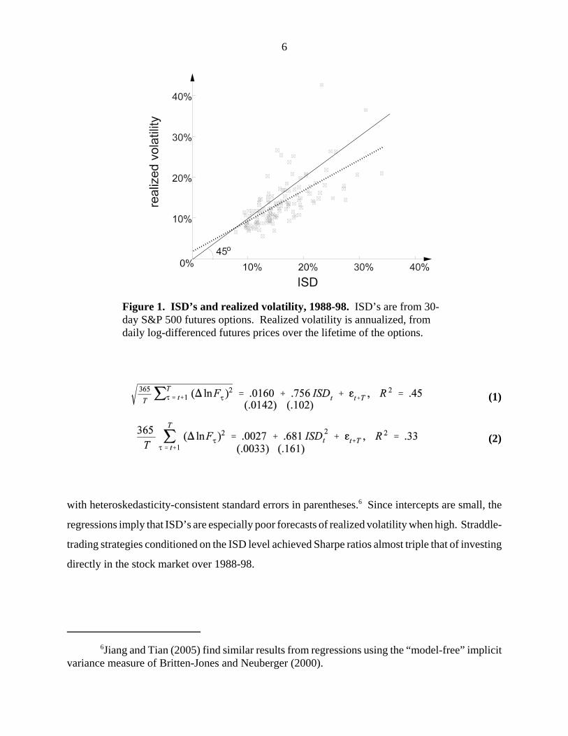
The conditional volatility puzzle is that regressing realized volatility upon ISD’s generally

yields slopes that are significantly positive, but significantly less than one. For instance, the

regressions using the 30-day ISD’s and realized volatilities mentioned above yield volatility and

variance results

6

6Jiang and Tian (2005) find similar results from regressions using the “model-free” implicitvariance measure of Britten-Jones and Neuberger (2000).

(1)

(2)

Figure 1. ISD’s and realized volatility, 1988-98. ISD’s are from 30-day S&P 500 futures options. Realized volatility is annualized, fromdaily log-differenced futures prices over the lifetime of the options.

with heteroskedasticity-consistent standard errors in parentheses.6 Since intercepts are small, the

regressions imply that ISD’s are especially poor forecasts of realized volatility when high. Straddle-

trading strategies conditioned on the ISD level achieved Sharpe ratios almost triple that of investing

directly in the stock market over 1988-98.

7

7In options research, implicit skewness is roughly measured by the shape of the volatility“smirk,” or pattern of ISD’s across different strike prices (“moneyness”). The skewness/maturityinteraction can be seen by examined by the volatility smirk at different horizons conditional uponrescaling moneyness proportionately to the standard deviation appropriate at different horizons. See,e.g., Bates (2000, Figure 4). Tompkins (2001) provides a comprehensive survey of volatility surfacepatterns, including the maturity effects.

Table 1Implicit jump parameters, and (risk-neutral) cumulants at 1- and 6-month horizons, 1988-98 estimates.Average jump size: -6.6%Jump standard deviation: 11.0%Jump intensity:

1-month cumulants

6-month cumulants

Average factor realizations: .0092; .0143.Conditional variance = ; skewness = ; excess kurtosis = .

The skewness puzzle is that the levels of skewness implicit in stock index options are

generally much larger in magnitude than those estimated from stock index returns – whether from

unconditional returns (Jackwerth, 2000) or conditional upon a time series model that captures salient

features of time-varying distributions (Rosenberg and Engle, 2002). Furthermore, implicit skewness

falls off only slightly for longer maturities of stock index options of, e.g., 3-6 months.7 By contrast,

the distribution of log-differenced stock indexes or stock index futures converges rapidly towards

near-normality as one progresses from daily to weekly to monthly holding periods.

8

Figure 2. Implicit factor estimates from S&P 500 futures options, 1988-98. V1 affects all cumulants, at all maturities. V2 affects conditional variance but has littleimpact on higher cumulants. Units are in instantaneous variance per year conditional on nojumps (left scale), or in implicit jump frequency (right scale). See Bates (2000) forestimation details.

A further puzzle is the evolution of distributions implicit in option prices. Figure 2

summarizes that evolution using updated estimates of the Bates (2000) 2-factor stochastic

volatility/jump-diffusion model with time-varying jump risk. The affine structure of that model

permits a factor representation of implicit cumulants in terms of two underlying state variables. The

first factor (V1) affects variance directly and also determines the jump intensity, thereby affecting

cumulants at all maturities. The second factor (V2) influences instantaneous variance (with roughly

half the variance loading of V1; see Table 1 above), but has relatively little impact on higher

cumulants.

9

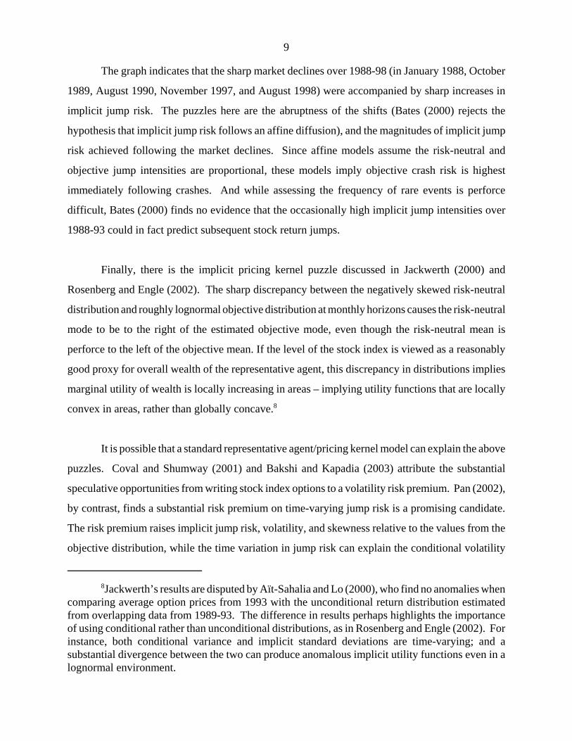
8Jackwerth’s results are disputed by Aït-Sahalia and Lo (2000), who find no anomalies whencomparing average option prices from 1993 with the unconditional return distribution estimatedfrom overlapping data from 1989-93. The difference in results perhaps highlights the importanceof using conditional rather than unconditional distributions, as in Rosenberg and Engle (2002). Forinstance, both conditional variance and implicit standard deviations are time-varying; and asubstantial divergence between the two can produce anomalous implicit utility functions even in alognormal environment.

The graph indicates that the sharp market declines over 1988-98 (in January 1988, October

1989, August 1990, November 1997, and August 1998) were accompanied by sharp increases in

implicit jump risk. The puzzles here are the abruptness of the shifts (Bates (2000) rejects the

hypothesis that implicit jump risk follows an affine diffusion), and the magnitudes of implicit jump

risk achieved following the market declines. Since affine models assume the risk-neutral and

objective jump intensities are proportional, these models imply objective crash risk is highest

immediately following crashes. And while assessing the frequency of rare events is perforce

difficult, Bates (2000) finds no evidence that the occasionally high implicit jump intensities over

1988-93 could in fact predict subsequent stock return jumps.

Finally, there is the implicit pricing kernel puzzle discussed in Jackwerth (2000) and

Rosenberg and Engle (2002). The sharp discrepancy between the negatively skewed risk-neutral

distribution and roughly lognormal objective distribution at monthly horizons causes the risk-neutral

mode to be to the right of the estimated objective mode, even though the risk-neutral mean is

perforce to the left of the objective mean. If the level of the stock index is viewed as a reasonably

good proxy for overall wealth of the representative agent, this discrepancy in distributions implies

marginal utility of wealth is locally increasing in areas – implying utility functions that are locally

convex in areas, rather than globally concave.8

It is possible that a standard representative agent/pricing kernel model can explain the above

puzzles. Coval and Shumway (2001) and Bakshi and Kapadia (2003) attribute the substantial

speculative opportunities from writing stock index options to a volatility risk premium. Pan (2002),

by contrast, finds a substantial risk premium on time-varying jump risk is a promising candidate.

The risk premium raises implicit jump risk, volatility, and skewness relative to the values from the

objective distribution, while the time variation in jump risk can explain the conditional volatility

10

(3)

bias. Bates (2000) finds that this model can also match the maturity profile of implicit skewness

better than models with constant implicit jump risk.

The challenges for these explanations are devising theoretical models of compensation for

risk consistent with the magnitude of the speculative opportunities. The stochastic evolution of

implicit jump risks from option prices also appears difficult to explain. The apparent magnitude and

evolution of the crash risk premium are the two central styled facts that I will attempt to match, in

the models below.

2. A jump-diffusion economy

I consider a simple continuous-time endowment economy over , with a single terminal

dividend payment at time T. News about this dividend (or, equivalently, about the terminal

value of the investment) arrives as a univariate Markov jump-diffusion of the form

where Z is a standard Wiener process,

N is a Poisson counter with constant intensity , and

is a deterministic jump size or announcement effect, assumed negative.

is the current signal about the terminal payoff and follows a martingale, implying

.

Financial assets are claims on terminal outcomes. Given the simple specification of news

arrival, any three non-redundant assets suffice to dynamically span this economy; e.g., bonds, stocks,

and a single long-maturity stock index option. However, it is analytically more convenient to work

with the following three fundamental assets:

1) a riskless numeraire bond in zero net supply that delivers one unit of terminal consumption

in all terminal states of nature;

2) an equity claim in unitary supply that pays a terminal dividend at time T, and is priced

at at time t relative to the riskless asset; and

11

(4)

(5)

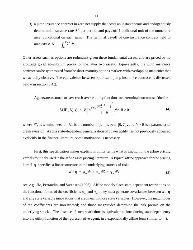
3) a jump insurance contract in zero net supply that costs an instantaneous and endogenously

determined insurance rate per period, and pays off 1 additional unit of the numeraire

asset conditional on each jump. The terminal payoff of one insurance contract held to

maturity is .

Other assets such as options are redundant given these fundamental assets, and are priced by no

arbitrage given equilibrium prices for the latter two assets. Equivalently, the jump insurance

contract can be synthesized from the short-maturity options markets with overlapping maturities that

we actually observe. The equivalence between optionsand jump insurance contracts is discussed

below in section 3.4.2.

Agents are assumed to have crash-averse utility functions over terminal outcomes of the form

where is terminal wealth, is the number of jumps over , and is a parameter of

crash aversion. As this state-dependent generalization of power utility has not previously appeared

explicitly in the finance literature, some motivation is necessary.

First, this specification makes explicit in utility terms what is implicit in the affine pricing

kernels routinely used in the affine asset pricing literature. A typical affine approach for the pricing

kernel specifies a linear structure in the underlying sources of risk:

see, e.g., Ho, Perraudin, and Sørensen (1996). Affine models place state-dependent restrictions on

the functional forms of the coefficients and ; they must generate covariances between

and any state variable innovations that are linear in those state variables. However, the magnitudes

of the coefficients are unrestricted; and those magnitudes determine the risk premia on the

underlying shocks. The absence of such restrictions is equivalent to introducing state dependency

into the utility function of the representative agent, in a exponentially affine form similar to (4).

12

9As illustrated in Basak (2000), models with heterogeneous subjective beliefs can besubstantially harder to solve than the utility-based approach used here.

(6)

A related justification is revealed preference – the derivation of utility functions consistent

with observed risk premia. The prices of all risks in a traditional representative-agent power utility

specification depend upon the risk aversion parameter , constraining the ability of such models

to simultaneously match the equity premium and the crash risk premium. The above utility function

can be derived as the entropy-minimizing pricing kernel that generates specific instantaneous equity

and jump risk premia, when returns are generated by an i.i.d jump-diffusion process. Conversely,

the ability of the above utility specification to generate equity and crash risk premia will be apparent

below.

Perhaps the most intuitive justification is that the crash aversion parameter can be viewed

a utility-based proxy for subjective beliefs about crash risk. Investors with crash-averse preferences

( ) are equivalent to investors with state-independent preferences and a subjective belief that

the jump intensity is :

This reflects the general proposition that preferences and beliefs are indistinguishable in a terminal

exchange economy. It should be recognized, however, that this interpretation involves very strong

subjective beliefs, in that investors do not update their subjective jump intensities based on

learning over time, or based on trading with other investors in the heterogeneous-agent equilibrium

derived below.9

A final justification is provided by Liu, Pan, and Wang (2004), who derive the utility

specification (4) from robust control methods given uncertainty aversion to the estimate of the jump

intensity. It is also worth noting that (4) is a utility specification with convenient properties. It

retains the homogeneity of standard power utility, and the myopic investment strategy property of

the log utility subcase .

13

10A crash insurance contract with instantaneous cost that pays off 1 unit of thenumeraire conditional upon a jump occurring in is priced at

yielding the above expression.

(7)

(8)

The above is a model of “external” crash aversion: investors are averse to bad news shocks.

An alternate “internal” crash aversion model could be constructed assuming investors’ aversion to

crashes depends on the degree to which their own investments are directly affected:

where is the jump in log wealth conditional upon a jump occurring, and conditional upon the

investor’s portfolio allocation. The major advantage to the external crash aversion in (4) is its

analytic tractability. While it is possible to work out homogeneous-agent equilibria using internal

crash aversion, deriving heterogeneous-agent equilibria is trickier. The difference in specifications

echoes the analytic advantages of external over internal habit formation models discussed in

Campbell, Lo and MacKinlay (1997, p. 327-8).

2.1 Equilibrium in a homogeneous-agent economy

The fundamental equations for pricing equity and crash insurance are

where is a nonnegative pricing kernel. The first two equations are standard; see, e.g.,

Grossman and Zhou (1996). The last is derived in Bates (1988, 1991).10 If all agents have identical

crash-averse preferences of the form given in (4) above, the pricing kernel can be derived from the

terminal marginal utility:

14

(9)

(10)

(11)

(12)

(13)

(14)

The following lemma is useful for computing relevant conditional expectations.

Lemma: If follows the jump-diffusion in (3) above and is the underlying jump counter

with intensity , then

Proof: For , there is a probability of observing n jumps

over . Conditional upon n jumps, , and

The last line follows from the independence of the Wiener and jump components, and from the

moment generating functions for Wiener and jump processes. O

Using the lemma, equations (8), and yields the following asset

pricing equations:

15

(15)

(16)

(17)

(18)

The last equation implies that the price of equity relative to the riskless numeraire follows

roughly the same i.i.d. jump-diffusion process as the underlying news about terminal value, with

identical instantaneous volatility and jump magnitudes:

for . The instantaneous equity premium

reflects required compensation for two types of risk. First is the required compensation for stock

market variance from diffusion and jump components, roughly scaled by the coefficient of relative

risk aversion. Second, the crash aversion parameter increases the required excess return when

stock market jumps are negative.

Crash aversion also directly affects the price of crash insurance relative to the actual arrival

rate of crashes:

Finally, derivatives are priced as if equity followed the risk-neutral martingale

where is a jump counter with constant intensity . The resulting (forward) option prices are

identical to the deterministic-jump special case of Bates (1991), given the geometric jump-diffusion.

2.2 Consistency with empirical anomalies

The homogeneous crash aversion model can explain some of the stylized facts from section 1. First,

unconditional bias in implied volatilities is explained by the potentially substantial divergence

between the risk-neutral instantaneous variance implicit in option prices, and the actual

instantaneous variance of log-differenced asset prices. Second, the difference between

and is consistent with the observation in Bates (2000, pp. 220-1) and Jackwerth (2000, pp.

16

(19)

446-7) of too few observed jumps over 1988-98 relative to the number predicted by stock index

options. The extra parameter permits greater divergence in from than is feasible under

standard parameterizations of power utility.

To illustrate this, consider the following calibration: a stock market volatility = 15%

annually conditional upon no jumps, and adverse news of that arrives on average once

every four years ( ). From equations (16) and (17), the equity premium and crash insurance

premium are

For R = 1 and Y = 1, the equity premium is 5%/year, while the jump risk implicit in option prices

is three times that of the true jump risk. Thus, the crash aversion parameter Y is roughly as

important as relative risk aversion for the equity premium, but substantially more important for the

crash premium. Achieving the observed substantial disparity between and 8 using risk aversion

alone would require levels of R that most would find unpalatable, and which would imply

an implausibly high equity premium.

Since returns are i.i.d. under both the actual and risk-neutral distribution, the homogeneous-

agent model is not capable of capturing the dynamic anomalies discussed in section 1. The standard

results from regressing realized on implicit variance cannot be replicated here, because neither is

time-varying in this model. Were there a time-varying volatility component in the news process,

however, the difference between and would affect the intercept from such regressions but

could not explain why the slope estimate is less than 1. Second, the model cannot match the

observed tendency of to jump contemporaneously with substantial market drops. Finally, the

i.i.d. return structure implies that implicit distributions should rapidly converge towards

lognormality at longer maturities, which does not accord with the maturity profile of the volatility

smirk.

Furthermore, Jackwerth’s (2000) anomaly cannot be replicated under homogeneous crash

aversion. As discussed in Rosenberg and Engle (2002), Jackwerth’s implicit pricing kernel involves

17

(20)

(21)

the projection of the actual pricing kernel upon asset payoffs. E.g., stock index options with

terminal payoff have an initial price

where has the usual properties of pricing kernels: it is nonnegative, and .

It is shown in the appendix that for crash-averse preferences, this projection takes the form

where is a function of time and is the probability density function of conditional

upon a jump intensity of over (0, t). Implicit relative risk aversion is given by .

For , one observes the strictly decreasing pricing kernel and constant relative risk aversion

associated with power utility. For , it is proven in the appendix that is a strictly

decreasing function of that is illustrated below in Figure 3. Thus, this pricing kernel cannot

replicate the negative implicit risk aversion (positive slope) estimated by Jackwerth (2000) and

Rosenberg and Engle (2002) for some values of . However, crash-averse preferences can replicate

the higher implicit risk aversion (steeper negative slope) for low values that was estimated by

those authors and by Aït-Sahalia and Lo (2000).

Jackwerth (2000, p.446) conjectures that the negative risk aversion estimate may be

attributable to investors overestimating the crash risk relative to the observed ex post crash

frequency. Within this model, such overestimation is equivalent to a positive value of , and cannot

generate the required divergences between objective and risk-neutral distributions. In equilibrium

the equity premium (16) is also positively affected by Y, shifting the mode of the objective

18

(22)

distribution sufficiently to the right to preclude observing Jackwerth’s anomaly. Of course, there

could still be an anomalous disparity between the risk-neutral distribution and the estimate of the

objective distribution.

Jackwerth’s exploration of whether the divergence between the risk-neutral and estimated

objective distributions is implausibly profitable is a separate issue. Within this framework, crash

aversion can generate investment opportunities with high Sharpe ratios. For instance, the

instantaneous Sharpe ratio on writing crash insurance is

which can be substantially larger than the instantaneous Sharpe ratio on equity given

investors’ aversion to this type of risk. The put selling strategies examined in Jackwerth implicitly

involve a portfolio that is instantaneously long equity and short crash insurance. Since adding a high

Sharpe ratio investment to a market investment must raise instantaneous Sharpe ratios, this model

is consistent with the substantial profitability of option-writing strategies reported in Jackwerth

(2000) and elsewhere.

-0.3 -0.2 -0.1 0.1 0.2 0.3

0.5

1

1.5

2

Figure 3. Log of the implicit pricing kernel conditional upon realized returns. Calibration:t = 1/12, , , .

19

(23)

(24)

3. Equilibrium in a heterogeneous-agent economy

As this model is dynamically complete, equilibrium in the heterogeneous-agent case can be

identified by examining an equivalent central planner’s problem in weighted utility functions. The

solution to that problem is Pareto-optimal, and can be attained by a competitive equilibrium for

traded assets in which all investors willingly hold market-clearing optimal portfolios given

equilibrium asset price evolution. Section 3.1 below outlines the central planner’s problem, while

Section 3.2 discusses the resulting asset market equilibrium. Section 3.3 identifies the supporting

individual wealth evolutions and associated portfolio allocations, and confirms the optimality of the

equilibrium. Section 3.4 discusses the implications for option prices, while Section 3.5 compares

the equilibrium with the stylized facts discussed above in Section 1.

3.1 The central planner’s problem

For analytic tractability, I will assume all investors have common risk aversion R, but differ in crash

aversion Y. Under common beliefs about state probabilities, the central planner’s problem of

maximizing a weighted average of expected state-dependent utilities is equivalent to constructing

a representative state-dependent utility function in terminal wealth (Constantinides 1982, Lemma

2):

for fixed weights that depend upon the initial wealth allocation in a fashion determined

below in Section 3.3. Since the individual marginal utility functions at

and the horizon is finite, the individual no-bankruptcy constraints are non-binding

and can be ignored. Optimizing the Lagrangian

yields a terminal state-dependent wealth allocation

20

(25)

(26)

(27)

(28)

(29)

and a Lagrangian multiplier

where is a CES-weighted average of individual crash aversion functions ’s. The Lagrangian

multiplier is the shadow value of terminal wealth, and therefore determines

the pricing kernel when evaluated at . From the first-order conditions to (24), all

individual terminal marginal utilities of wealth are directly proportional to the multiplier:

3.2 Asset market equilibrium

As in equations (8) above, the pricing kernel can be used to price all assets. That asset

market equilibrium depends critically upon expectations of average crash aversion. Define

as the conditional expectation of given jump intensity over for future jumps

. It is shown in the appendix that the resulting asset pricing equations are

21

(30)

(31)

(32)

(33)

(35)

(34)

where and .

The equilibrium equity price follows a jump-diffusion of the form

where

and

for defined above in equation (30). The risk-neutral price process follows a martingale of

the form

for a risk-neutral jump counter with instantaneous jump intensity , the functional form

of which is given above in equation (31).

Several features of the equilibrium are worth emphasizing. First, conditional upon no jumps

the asset price follows a diffusion similar to the news arrival process – i.e., with identical and

22

11Dieckmann and Gallmeyer (2005) find that heterogeneous risk aversion increases stockmarket volatility relative to the underlying sources of risk.

(36)

(37)

(38)

(39)

constant instantaneous volatility . This property reflects the assumption of common relative risk

aversion R, and would not hold in general under alternate utility specifications or heterogeneous risk

aversion.11 A further implication discussed below is that all investors hold identical equity positions.

Second, the equilibrium price process and crash insurance premium depend critically upon

the heterogeneity of agents. This is simplest to illustrate in the case, for which equilibrium

values can be expressed directly in terms of the weighted distribution of individual crash aversions.

Define pseudo-probabilities

as the weight assigned to investors of type at time t, and define cross-sectional average ,

variance , and covariance with respect to those weights. It is shown in the appendix that

the asset market equilibrium takes the form

To a first-order approximation, jump insurance premia in (37) and equity prices in (38)

replicate the homogeneous-agent equilibria of (12) and (14) at , using average values for Y

and , respectively. However, heterogeneity introduces second- and higher-order effects, as well,

depending upon the dispersion of agents. In particular, the size of log equity jumps in (34)

and (39) can be substantially magnified relative to the adverse news shock about terminal value

23

0.2 0.4 0.6 0.8 1

-0.175

-0.15

-0.125

-0.1

-0.075

-0.05

-0.025

0.2 0.4 0.6 0.8 1

1.25

1.5

1.75

2

2.25

2.5

2.75

0.2 0.4 0.6 0.8 1

0.05

0.06

0.07

0.08

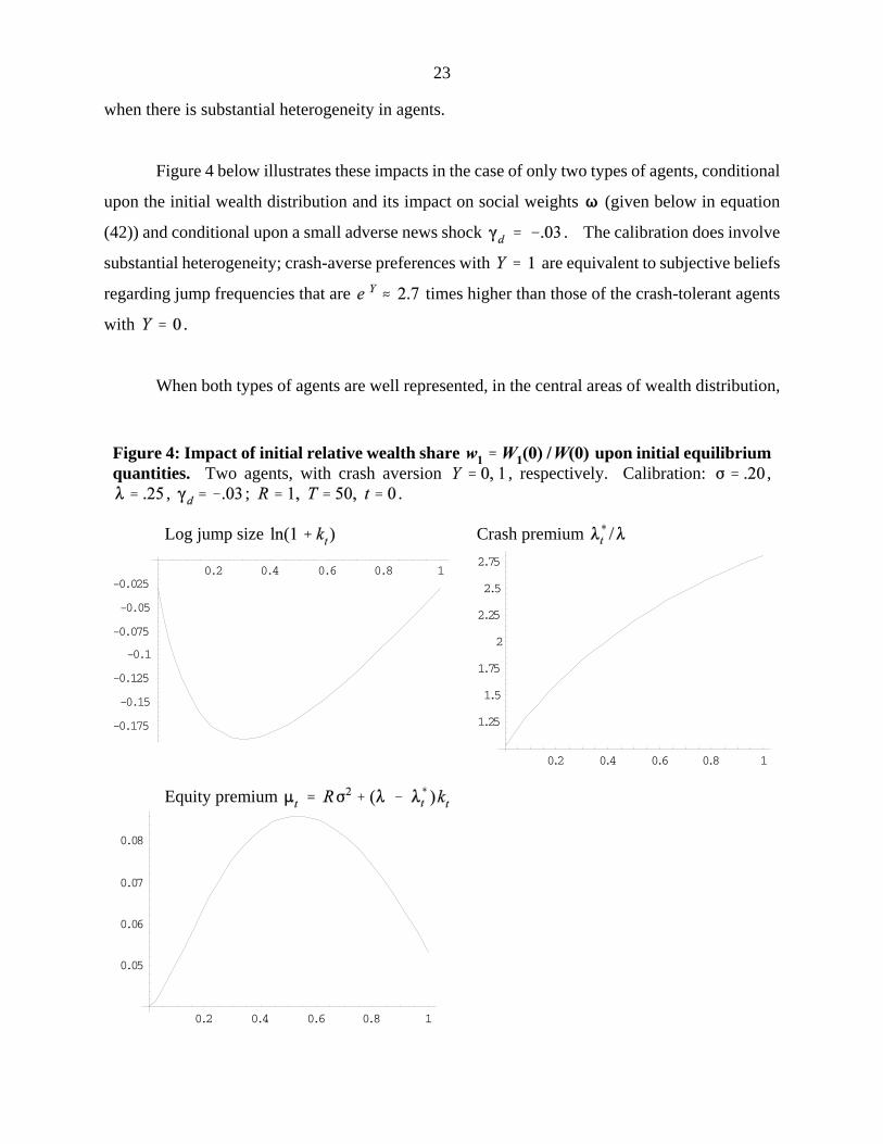
Figure 4: Impact of initial relative wealth share upon initial equilibriumquantities. Two agents, with crash aversion , respectively. Calibration: ,

, ; .

Log jump size Crash premium

Equity premium

when there is substantial heterogeneity in agents.

Figure 4 below illustrates these impacts in the case of only two types of agents, conditional

upon the initial wealth distribution and its impact on social weights (given below in equation

(42)) and conditional upon a small adverse news shock . The calibration does involve

substantial heterogeneity; crash-averse preferences with are equivalent to subjective beliefs

regarding jump frequencies that are times higher than those of the crash-tolerant agents

with .

When both types of agents are well represented, in the central areas of wealth distribution,

24

Table 2. Average log jump size conditional upon initial wealth allocation and risk aversion R. Calibration: , , , .

given: R

.5 1 2 4 8

0 .0001 .001 .01 .1 .2 .3 .4 .5 .6 .7 .8 .9 .99 .9991

-.030-.030-.032-.052-.157-.189-.187-.171-.149-.125-.101-.076-.053-.032-.030-.030

-.030-.030-.032-.045-.136-.178-.189-.183-.166-.144-.118-.090-.060-.033-.030-.030

-.030-.030-.030-.036-.090-.135-.163-.177-.178-.169-.149-.119-.079-.035-.030-.030

-.030-.030-.030-.031-.044-.061-.079-.097-.114-.128-.135-.129-.096-.035-.030-.030

-.030-.030-.030-.030-.034-.038-.043-.048-.053-.059-.066-.072-.065-.033-.030-.030

there is a substantial impact of small announcements upon jumps in log equity prices. The

divergence of preferences implies substantial trading of crash insurance, and substantial wealth

redistribution and shifts in the investment opportunity set conditional upon a jump. The result is that

a modest 3% drop in the terminal value signal can induce a 3% to 18% drop in the log price of

equity. Crashes redistribute wealth, making the “average” investor more crask-averse and

exacerbating the impact of adverse news shocks. As indicated in Table 2 below, this magnification

is also present for alternate values of the risk aversion parameter R.

The crash insurance rate is always between the value of the crash-tolerant

investors ( ), and the value of the crash-averse investors. Its value depends

monotonically upon the relative weights of the two types of investors, and is biased upward relative

to the wealth-weighted average by the variance term in equation (37). The equity premium varies

somewhat with the magnitude of crash risk, in a non-monotonic fashion.

25

12See Dumas (1989) and Wang (1996) for examples of the predominantly nonstationaryimpact of heterogeneity in a diffusion context. An interesting exception is Chan and Kogan (2002),who show that external habit formation preferences can induce stationarity in an exchange economywith heterogeneous agents.

(40)

(41)

A final observation is that the asset market equilibrium depends upon the number of jumps

, and is consequently nonstationary. This is an almost unavoidable feature of equilibrium models

with a fixed number of heterogeneous agents. Heterogeneity implies agents have different portfolio

allocations, implying their relative wealth weights and the resulting asset market equilibrium depend

upon the nonstationary outcome of asset price evolution.12 In this model, the number of jumps

and time t are proxies for wealth distribution. Crashes redistribute wealth towards the more crash-

averse, making the representative agent more crash-averse. An absence of crashes has the opposite

effect through the payment of crash insurance premia.

3.3 Supporting wealth evolution and portfolio choice

An investor’s wealth at any time t can be viewed as the value (or cost) of a contingent claim that

pays off the investor’s share of terminal wealth conditional upon the number of jumps:

see equation (A.16) in the appendix for details. The quantity is the current share of

current total wealth , and appropriately sums to 1 across all investors. The weights of

the social utility function are implicitly identified up to an arbitrary factor of proportionality by the

initial wealth distribution:

26

(42)

(43)

(44)

for . In the case the mapping between and the initial wealth

distribution is explicit, and takes the form

The investment strategy that dynamically replicates the evolution of can be identified

using positions in equity and crash insurance that mimic the diffusion- and jump-contingent

evolution:

where is the percentage jump size in the equity price given above in equations (34) and

(39). Thus, each investor holds shares of equity (i.e., is 100% invested in equity),

and holds a relative crash insurance position of

The wealth-weighted aggregate crash insurance positions appropriately sum

to 0.

Figure 5 below graphs the individual crash insurance demands given crash aversions

and 1, respectively, conditional upon the initial wealth allocation and its

impact upon equilibrium . The aggregate demand for crash insurance is also graphed,

using the same calibration as in Figure 4 above. At , crash-tolerant investors set a

relatively low market-clearing price and sell little insurance. Crash-averse investors

insure heavily individually, but are a negligible fraction of the market. As increases,

does as well (see Figure 4 above) and the crash insurance positions of both investors decline.

Aggregate crash insurance volumes are heaviest in the central regions where both types of investors

are well represented. As approaches 1, the high price of crash insurance induces crash-tolerant

27

0.2 0.4 0.6 0.8 1

-0.5

0.5

1

1.5

Figure 5. Equilibrium crash insurance positions andaggregate demand for crash insurance, as a function of

. Calibration is the same as in Figure 4.

Crash-averse investors’

Total demand

Crash-tolerant investors’

investors to sell insurance that will cost them 60% of their wealth conditional upon a crash.

3.3.1 Optimality

The individual’s investment strategy yields a terminal wealth , and an associated terminal

marginal utility of wealth that (from equation (27)) is proportional to the

Lagrangian multiplier that prices all assets. Therefore, no investor has an incentive to perturb

his investment strategy given equilibrium asset prices and price processes. Furthermore, as noted

above, the markets for equity and crash insurance clear, so the markets are in equilibrium. Since

all individual state-dependent marginal utilities are proportional at expiration, the market is

effectively complete. All investors agree on the price of all Arrow-Debreu securities, so their

introduction would not affect the equilibrium.

3.3.2 Comparison with myopic investment strategies

The equilibrium asset price evolution in Section 3.2 involves considerable and stochastic evolution

over time of the instantaneous investment opportunity set. Since Merton (1973), hedging against

such shifts has been identified as the key distinction between static and dynamic asset market

equilibria. As there are conflicting results even in a diffusion setting as to the quantitative

28

13Campbell and Viceira (1999) and Campbell, Chacko, Rodriguez and Viceira (2004) findsubstantial hedging against stochastic shifts in expected returns, while Chacko and Viceira (2005)find little hedging against stochastic volatility. The two approaches diverge in the specification andcalibration of shifts in the investment opportunity set.

(45)

(47)

importance of such hedging,13 and as there has been little exploration of the issue in a jump-diffusion

context, a comparison with the myopic investment strategies characteristic of static equilibria may

be useful. Furthermore, myopic strategies are optimal when investors have unitary risk aversion

( ), or when returns are i.i.d. – e.g., in the case of investor homogeneity.

The myopic portfolio allocation is defined as the position that maximizes terminal expected

utility

conditional upon assuming instantaneous investment opportunities will remain unchanged at the

current level over the investor’s lifetime. Those opportunities are summarized by the instantaneous

cost of crash insurance , and the price process

No assumptions are made at this stage regarding the values of .

It is shown in the appendix that the myopic investor will choose constant portfolio proportions

where is the portfolio share in equity, and

is the number of insurance contracts as a fraction of overall wealth.

If investors are homogeneous, the market-clearing conditions yield the

equilibrium and time-invariant given above in equations (12) and (16). The above myopic

portfolio weights are also optimal under time-varying when , but not for general

29

R.

The myopic portfolio allocation equations (47) indicate that equity and crash insurance are

complements when jumps are negative ( ). An increase in the price of crash insurance

lowers the demand for both equity and crash insurance, while an increase in the expected excess

return on equity raises both. The equations also indicate that myopic crash insurance positions

but not equity positions are directly affected by the investor’s idiosyncratic crash aversion parameter

. Furthermore, at the equilibrium equity premium (33), myopic investors duplicate the optimal

investment strategy of holding 100% in equity, and diverge from that optimum only in their holdings

of crash insurance.

Table 3 compares the optimal and myopic crash insurance strategies at the equilibrium values

for resulting from various initial wealth allocations and risk aversion. The two strategies

are broadly similar across different asset market equilibria, and are identical either when risk

aversion , or when a preponderance of one type of individual ( . 0 or 1) yields a

homogeneous-agent equilibrium with a time-invariant investment opportunity set.

The table indicates that a myopic strategy can be a poor approximation to the optimal

strategy in other cases. The divergence is most pronounced for the large positions achieved under

low levels of risk aversion , but is also present for larger R values. For instance, when

crash-tolerant and crash-averse investors are equally represented ( = ½) and R = 2, a 3%

adverse news shock will induce a 17.8% stock market crash (from Table 2). The crash-averse buy

crash insurance contracts from the crash-tolerant that pay off 36.5% of current wealth conditional

on a crash. The myopic positions = (-16.9%, 26.4%) in Table 3 substantially

understate the magnitude of those optimal insurance positions.

30

Table 3. Optimal and myopic crash insurance positions, at equilibrium asset prices determined byidiosyncratic crash aversions , initial wealth allocation , and common riskaversion R. Equilibrium values for and parameter values are in Table 2 above. Entries indicatethe payoff of insurance positions conditional on a crash, as a fraction of investor’s wealth.

Crash aversion ; R = Crash aversion ; R =

0.5 1 2 4 8 0.5 1 2 4 8

Optimal positions

0.0.0001.001.01.1.2.3.4.5.6.7.8.9.99.999

1.0

.000 .000-.002-.017-.128-.215-.285-.347-.402-.452-.499-.542-.584-.629-.651-.839

.000 .000-.002-.016-.128-.214-.282-.339-.391-.440-.485-.529-.572-.609-.613-.613

.000 .000-.001-.011-.119-.205-.270-.321-.365-.405-.444-.482-.518-.497-.418-.382

.000 .000 .000-.003-.062-.140-.204-.255-.293-.322-.341-.352-.345-.241-.217-.215

.000 .000 .000-.001-.017-.045-.080-.115-.145-.166-.177-.175-.153-.118-.114-.114

6.2001.8521.7731.6481.148 .858 .666 .520 .402 .301 .214 .136 .065 .006 .001 .000

1.6671.6671.6601.5981.152 .856 .657 .509 .391 .293 .208 .132 .064 .006 .001 .000

.630 .652 .793

1.1341.069 .822 .629 .482 .365 .270 .190 .121 .058 .005 .000 .000

.276

.276

.277

.299

.557

.559

.477

.382

.293

.214

.146

.088

.038

.002

.000

.000

.129

.129

.129

.131

.152

.179

.187

.173

.145

.111

.076

.044

.017

.001

.000

.000

Myopic positions

0.0.0001.001.01.1.2.3.4.5.6.7.8.9.99.999

1.0

.000 .000-.004-.041-.284-.429-.522-.592-.648-.695-.737-.774-.808-.836-.839-.839

.000 .000-.002-.016-.128-.214-.282-.339-.391-.440-.485-.529-.572-.609-.613-.613

.000 .000-.001-.007-.056-.091-.117-.142-.169-.199-.234-.275-.324-.376-.381-.382

.000 .000 .000-.002-.028-.051-.066-.073-.077-.080-.087-.103-.142-.209-.214-.215

.000 .000 .000-.001-.010-.021-.032-.041-.048-.053-.055-.058-.072-.110-.114-.114

6.2006.1956.1535.7643.3622.1221.4401.012 .717 .501 .334 .201 .092 .008 .001 .000

1.6671.6671.6601.5981.152 .856 .657 .509 .391 .293 .208 .132 .064 .006 .001 .000

.630

.629

.628

.615

.500

.418

.358

.309

.264

.220

.173

.122

.065

.007

.001

.000

.276

.276

.275

.272

.236

.201

.178

.164

.154

.147

.137

.117

.075

.006

.001

.000

.129

.129

.129

.128

.117

.104

.091

.080

.071

.066

.062

.058

.043

.004

.000

.000

31

(48)

(49)

(50)

3.4 Option markets

3.4.1 Option prices

At time 0, European call options of maturity are priced at expected terminal value weighted by

the pricing kernel:

Conditional upon jumps over , and have a joint lognormal distribution that reflects

their common dependency on given above in equations (29) and (30). Consequently, it is shown

in the appendix that the risk-neutral distribution for is a weighted mixture of lognormals,

implying European call option prices are a weighted average of Black-Scholes-Merton prices:

where ,

,

,

and

.

Put prices can be computed from call prices using put-call parity:

Since jumps are always negative, the distribution of log-differenced equity prices implicit

in option prices is always negatively skewed. The maturity profile of implicit skewness is quite

sensitive to the initial distribution of wealth, given the nonmonotonic dependency of on

wealth distribution shown above in Table 2 and Figure 4. For small values of , a second jump

will be larger than the first. The increasing probability of multiple jumps at longer maturities causes

implicit skewness to fall slower than the rate of i.i.d. returns, implying slower flattening out

of the implicit volatility smirk. For larger values of the size of sequential jump sizes is reversed,

32

14Tompkins examines implicit volatility patterns from various countries’ futures options oncurrency, stock index, bonds and interest rates, with the moneyness dimension appropriately scaledby maturity-specific volatility estimates from at-the-money options. He finds some maturityvariation in implicit volatility patterns, but not much by comparison with the strong inverse patternpredicted by i.i.d. returns.

0.2 0.4 0.6 0.8 1

-0.12

-0.08

-0.06

-0.04

-0.02

Figure 6. Annualized risk-neutral skewness, as a function of t.

and implicit skewness can fall faster than the rate of i.i.d. returns; see Figure 6.

However, model-specific estimates from option prices such as in Table 1 above indicate that

implicit (rather than ) is roughly flat across option maturities t. This stylized

fact appears common to a broad array of futures options, as indicated in the Tompkins (2000) survey

of volatility smiles and smirks.14 Thus, although Bates (2000) argues that stochastic implicit jump

intensities are needed to match the volatility smirk at longer maturities, it does not appear that

the stochastic variation of in this model generates the correct maturity profile of implicit

skewness.

3.4.2 Option replication and dynamic completion of the markets

Options can be dynamically replicated using positions in equity and crash insurance. Instanta-

neously, each call option has a price , and can be viewed as an instantaneous bundle of

units of equity risk, and units of crash insurance.

33

15As indicated above in Figure 4, the total volume (open interest) in crash insurance andtherefore in options can either rise or fall as the wealth distribution varies.

This equivalence between options and crash insurance indicates how investors replicate the

optimal positions of section 3.3 dynamically using the call and/or put options actually available.

Crash-averse investors choose an equity/options bundle with unitary delta overall and positive

gamma (e.g., hold 1½ stocks and buy one at-the-money put option with a delta of -½), while crash-

tolerant investors take offsetting positions that also possess unitary delta (e.g., hold ½ stock, and

write 1 put option). Equity and option positions are adjusted in a mutually acceptable and offsetting

fashion over time, conditional upon the arrival of news. As options expire, new options become

available and investors are always able to maintain their desired levels of crash insurance. All

investors recognize that the price of crash insurance implicit in option prices will evolve over time,

conditional on whether crashes do or do not occur, and take that into account when establishing their

positions.

A further implication is that the crash-tolerant investors who write options actively delta-

hedge their exposure, which is consistent with the observed practice of option market makers. As

increases (e.g., because of wealth transfers to the crash-averse from crashes) , the market makers

respond to the more favorable prices by writing more options as a proportion of their wealth.15 They

simultaneously adjust their equity positions to maintain their overall target delta of 1. This strategy

is equivalent to market makers putting their personal wealth in an index fund, and fully delta-

hedging every index option they write.

3.5 Consistency with empirical option pricing anomalies

The heterogeneous-agent model explains unconditional deviations between risk-neutral and

objective distributions analogously to the homogeneous-agent model. The divergence in the jump

intensity implicit in options and the true jump frequency can reconcile the average divergence

between risk-neutral and objective variance, and between the predicted and observed frequency of

jumps over 1988-98. The heterogeneous-agent model can also be somewhat more consistent with

the maturity profile of implicit skewness than the homogeneous-agent model, although still appears

inadequate relative to observed patterns.

34

2 4 6 8 10

0.0425

0.045

0.0475

0.05

0.0525

0.055

0.0575

0.06

Figure 7. Simulated instantaneous risk-neutral variance conditional upon jump timing matching that

observed over 1988-98. Calibration: ; i.e.,crash-averse investors own 10% of total wealth at end-1987.

The advantage of the heterogeneous-agent model is that it can explain some of the

conditional divergences as well. First, the stochastic evolution of is qualitatively consistent with

the evolution of jump intensity proxy V1 shown above in Figure 2. depends directly upon the

relative wealth distribution, which in turn follows a pure jump process given above in (41) for the

case. Consequently, market jumps cause sharp increases in , while an absence of jumps generates

geometric decay in towards the lower level of crash-tolerant investors.

Figure 7 below illustrates the resulting evolution of instantaneous risk-neutral variance

( ) conditional on the five major shocks over 1988-98, and conditional on starting with

= .1 at end-1987. This behavior is qualitatively similar to the actual impact of jumps on overall

variance and on jump risk shown above in Figure 2. However, the absence of major shocks over

1992-96 and the resulting wealth accumulation by crash-tolerant investors/option market makers

implies that the shocks of 1997 and 1998 should not have had the major impact that was in fact

observed.

It is possible the heterogeneous model can explain the results from ISD regressions as well.

The analysis is complicated by the fact that instantaneous objective and risk-neutral variance are

35

(51)

(52)

-0.3 -0.2 -0.1 0.1 0.2 0.3

-0.2

0.2

0.4

0.6

Figure 8. Log of the implicit pricing kernelconditional upon realized asset returns. Calibration: .

nonstationary, with a nonlinear cointegrating relationship from their common dependency on the

nonstationary variable :

for and . It is not immediately clear whether regressing realized on

implied volatility is meaningful under nonlinear cointegration. However, the fact that implicit

variance does contain information for objective variance but is biased upwards suggests that running

this sort of regression on post-’87 data would yield the usual informative-but-biased results reported

above in equation (2), with estimated slope coefficients less than 1 in sample.

It does not appear that the heterogeneous-agent model can explain the implicit pricing kernel

puzzle. Using the same projection as in (20) above , the projected pricing kernel is

As illustrated in Figure 8, this implicit pricing kernel appears to be a strictly decreasing

36

function of – in contrast to the locally positive sections estimated in Jackwerth (2000) and

Rosenberg and Engle (2002). However, the above implicit kernel can replicate those studies’ high

implicit risk aversion for large negative returns, as indicated by the slope of the line in Figure 8 for

in the -10% to -20% ranges.

4. Summary and conclusions

This paper has proposed a modified utility specification, labeled “crash aversion,” to explain the

observed tendency of post-’87 stock index options to overpredict realized volatility and jump risk.

Furthermore, the paper has developed a complete-markets methodology that permits identification

of asset market equilibria and associated investment strategies in the presence of jumps and investor

heterogeneity. The assumption of heterogeneity appears to have stronger consequences than

observed with diffusion models. Jumps can cause substantial reallocation of wealth, and the

resulting shifts in the investment opportunity set can be substantial. Small announcement effects

regarding the terminal value of the market can have substantially magnified instantaneous price

impacts when investors are heterogeneous.

The model has been successful in explaining some of the stylized facts from stock index

options markets. The specification of crash aversion is compatible with the tendency of option

prices to overpredict volatility and jump risk, while heterogeneity of agents offers an explanation

of the stochastic evolution of implicit jump risk and implicit volatilities. In this model, the two are

higher immediately after market drops not because of higher objective risk of future jumps (as

predicted by affine models), but because crash-related wealth redistribution has increased average

crash aversion. Crash aversion is also consistent with the implicit pricing kernel approach’s

assessment of high implicit risk aversion at low wealth levels, although the approach cannot

replicate the locally risk-loving behavior reported in Jackwerth (2000) and Rosenberg and Engle

(2002).

While motivated by empirical option price regularities, the model in the paper is not suitable

for direct estimation. First, jump risk is not the only risk spanned in the options markets. Stochastic

variations in conditional volatility occur more frequently, and are also important to option market

makers. Second, the nonstationary equilibrium derived here and characteristic of most

37

heterogeneous-agent models hinders estimation. The purpose of the paper is to provide a theoretical

framework for exploring the trading of jump risk through the options markets, as an initial model

of the option market making process. A more plausible model that might also resolve the

nonstationarity issue would be to include profit-taking by market makers, to limit their size in the

market.

The framework in this paper can be expanded in various ways. For simplicity, this paper has

focused on deterministic jumps and an “external” crash aversion specification insensitive to the

impact of crashes upon individual wealth. Extending the model to random jumps and/or “internal”

crash aversion should be relatively straightforward, although feedback effects in the latter case could

require additional restrictions to achieve an equilibrium. A particularly interesting extension could

be to explore the implications of portfolio constraints on positions in options and/or jump insurance.

Selling crash insurance requires writing calls or puts – a strategy that individual investors cannot

easily pursue. Further research will examine the impact of such constraints upon equilibria in equity

and options markets.

38

(A.1)

(A.2)

(A.3)

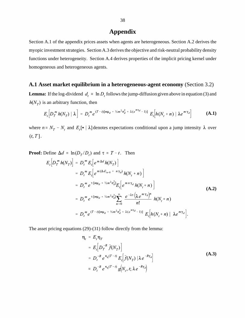
AppendixSection A.1 of the appendix prices assets when agents are heterogeneous. Section A.2 derives the

myopic investment strategies. Section A.3 derives the objective and risk-neutral probability density

functions under heterogeneity. Section A.4 derives properties of the implicit pricing kernel under

homogeneous and heterogeneous agents.

A.1 Asset market equilibrium in a heterogeneous-agent economy (Section 3.2)Lemma: If the log-dividend follows the jump-diffusion given above in equation (3) and

is an arbitrary function, then

where n and denotes expectations conditional upon a jump intensity over

.

Proof: Define and . Then

The asset pricing equations (29)-(31) follow directly from the lemma:

39

(A.4)

(A.5)

(A.6)

(A.7)

for and . Given

, can be written as .

In the special case and for arbitrary ,

Define and , and define pseudo-probabilities

Using (A.6) for g, the equity pricing equation (A.4) becomes

40

(A.8)

(A.9)

(A.10)

(A.11)

for the cross-sectional expectation defined with regard to probabilities (A.7), and for

. From (A.5), the jump risk premium has a similar

representation:

The approximation for the log jump size follows from the following approximations:

For , the partial derivatives of are

41

(A.12)

(A.13)

(A.14)

(A.15)

(A.16)

while the cross-derivative is

Consequently (from (A.11)),

Section 3.3, equation (40)

Substituting in from (A.4) yields (40).

42

(A.17)

(A.18)

(A.19)

(A.20)

(A.21)

A.2 Myopic portfolio choice (Section 3.3.2)The myopic portfolio allocation strategy in equity and crash insurance maximizes the

Hamilton-Jacobi-Bellman equation

under the assumption of constant , and subject to the terminal boundary condition

The first-order conditions to (A.17) with respect to q and x are

Given the terminal utility specification, it is straightforward to show that the value function J is of

the form

with an associated marginal utility function

Since and , this marginal utility function yields

constant portfolio proportions that satisfy

43

(A.22)

(A.23)

(A.24)

(A.25)

under a constant investment opportunity set. Furthermore, the value function and these portfolio

proportions satisfies the Hamilton-Jacobi-Bellman equation for some functions and that

appropriately converge to 1 as .

If , myopic investment strategies are optimal even if investment opportunities

are stochastic. Defining , the objective function becomes

where is a modified expectation conditional upon a jump intensity over .

Consequently, the marginal utility

is again of the form (A.21) above, and optimal portfolio proportions are given by (A.22) with .

A.3 Objective and risk-neutral distributionsStock prices and pricing kernels are jump-dependent multiples of the dividend signal, which is in

turn a draw from jump-dependent mixture of lognormals. From (30), gross stock returns are

for . The density function for is

44

(A.26)

(A.27)

(A.28)

(A.29)

(A.30)

for equal to the normal density function with mean m and variance . Consequently,

log-differenced stock prices are also drawn from a mixture of normals:

Define as the delta function that takes on infinite value when , zero value

elsewhere, and integrates to 1. The objective density function , while the risk-

neutral density function is

For any two normally distributed variables and and any arbitrary function ,

where is also normally distributed with mean and variance .

Conditional upon n jumps, and are both normally distributed with covariance .

Consequently, (A.28) can be re-written as

45

(A.31)

(A.32)

(A.33)

(A.34)

(A.35)

Since , the weights sum to 1. Furthermore, since

it is straightforward to show that

for .

A.4 Implicit pricing kernels (equations (21) and (52))Using equations (13) and (14), the projection of the pricing kernel upon the asset price in the

homogeneous-agent case is

where and capture time-dependent terms irrelevant to implicit risk aversion. The

distribution of is an -dependent mixture of normals:

Consequently, the conditional expectation in (A.33) can be evaluated using Bayes’ rule to evaluate

the conditional probabilities

46

(A.36)

(A.37)

(A.38)

yielding an implicit pricing kernel

where denotes the unconditional density of given a jump intensity of over .

Taking partials with respect to and using the fact that yields

(after some tedious calculations) an implicit risk aversion value

where and are defined with regard to the probabilities in (A.35). Since and n are

both increasing functions of n, the covariance term is positive. Consequently, the implicit risk

aversion is everywhere positive given .

The heterogeneous-agent case is similar. From (29) and (30), the Lagrange multiplier is

This is of the same form as (A.33), with replacing . Consequently, the

implicit pricing kernel becomes

47

(A.39)

for .

48

References

Aït-Sahalia, Yacine and Andrew W. Lo (2000). “Nonparametric Risk Management and ImpliedRisk Aversion.” Journal of Econometrics 94, 9-51.

Bakshi, Gurdip and Nikunj Kapadia (2003). “Delta-Hedged Gains and the Negative Volatility RiskPremium.” Review of Financial Studies 16, 572-566.

Back, Kerry (1993). “Asymmetric Information and Options.” Review of Financial Studies 6, 435-472.

Bardhan, Indrajit and Xiuli Chao (1996). “Stochastic Multi-Agent Equilibria In Economies withJump-Diffusion Uncertainty.” Journal of Economic Dynamics and Control 20, 361-384.

Basak, Suleyman (2000). “A Model of Dynamic Equilibrium Asset Pricing with HeterogeneousBeliefs and Extraneous Risk.” Journal of Economic Dynamics and Control 24, 63-95.

Basak, Suleyman and Domenico Cuoco (1998). “An Equilibrium Model with Restricted StockMarket Participation.” Review of Financial Studies 11, 309-341.

Bates, David S. (1988). “Pricing Options on Jump-Diffusion Processes.” Rodney L.White Centerworking paper 37-88.

Bates, David S. (1991). “The Crash of '87: Was It Expected? The Evidence from OptionsMarkets.” Journal of Finance 46, 1009-1044.

Bates, David S. (2000). “Post-'87 Crash Fears in the S&P 500 Futures Option Market.” Journal ofEconometrics 94, 181-238.

Britten-Jones, Mark and Anthony Neuberger (2000). “Option Prices, Implied Price Processes, andStochastic Volatility.” Journal of Finance 55, 839-866.

Campbell, John Y., Andrew W. Lo, and A. Craig MacKinlay (1997). The Econometrics of FinancialMarkets, Princeton, NJ: Princeton University Press.

Campbell, John Y., George Chacko, Jorge Rodriguez, and Luis M. Viceira (2004). “Strategic AssetAllocation in a Continuous-Time VAR Model.” Journal of Economic Dynamics and Control 28,2195-2214.

Campbell, John Y. and Luis M. Viceira (1999). “Consumption and Portfolio Decisions WhenExpected Returns are Time Varying.” Quarterly Journal of Economics , 433-495.

Chacko, George and Luis M. Viceira (2005). “Dynamic Consumption and Portfolio Choice withStochastic Volatility in Incomplete Markets.” Review of Financial Studies 18, 1369-1402.

49

Chan, Yeung Lewis and Leonid Kogan (2002). “Catching Up with the Joneses: HeterogeneousPreferences and the Dynamics of Asset Prices.” Journal of Political Economy 110, 1255-1285.

Coval, Joshua D. and Tyler Shumway (2001). “Expected Option Returns.” Journal of Finance 56,983-1009.

Dieckmann, Stephan and Michael Gallmeyer (2005). “The Equilibrium Allocation of Diffusive andJump Risks with Heterogeneous Agents. Journal of Economic Dynamics and Control 29, 1547-1576.

Dumas, Bernard (1989). “Two-Person Dynamic Equilibrium in the Capital Market.” Review ofFinancial Studies 2, 157-188.

Fleming, Jeff (1998). “The Quality of Market Volatility Forecasts Implied by S&P 100 IndexOption Prices.” Journal of Empirical Finance 5, 317-345.

Froot, Kenneth A. (2001). “The Market for Catastrophe Risk: A Clinical Evaluation.” Journal ofFinancial Economics 60, 529-571.

Grossman, Sanford J. and Zhongquan Zhou (1996). “Equilibrium Analysis of Portfolio Insurance.”Journal of Finance 51, 1379-1403.

Ho, Mun S., William R. M. Perraudin, and Bent E. Sorensen (1996). “A Continuous Time ArbitragePricing Model with Stochastic Volatility and Jumps.” Journal of Business and Economic Statistics14, 31-43.

Jackwerth, Jens Carsten (2000). “Recovering Risk Aversion from Option Prices and RealizedReturns.” Review of Financial Studies 13, 433-451.

Jiang, George and Yisong S. Tian (2005). “Model-Free Implied Volatility and Its InformationContent.” Review of Financial Studies 18, 1305-1342.

Liu, Jun, Jun Pan and Tan Wang (2005). “An Equilibrium Model of Rare Event Premia.” Reviewof Financial Studies 18, 131-164.

Merton, Robert C. (1973). “An Intertemporal Capital Asset Pricing Model.” Econometrica 41,867-887.

Pan, Jun (2002). “The Jump-Risk Premia Implicit in Options: Evidence from an Integrated Time-Series Study.” Journal of Financial Economics 63, 3-50.

Pan, Jun and Allen M. Poteshman (2005). “The Information in Option Volume for Future StockPrices.” MIT working paper, August 2005; forthcoming, Review of Financial Studies.

Rosenberg, Joshua and Robert F. Engle (2002). “Empirical Pricing Kernels.” Journal of FinancialEconomics 64, 341-372.

50

Santa-Clara, Pedro and Shu Yan (2005). “Crashes, Volatility, and the Equity Premium: Lessonsfrom S&P 500 Options.” UCLA working paper.

Tompkins, Robert G. (2000). “Implied Volatility Surfaces: Uncovering Regularities for Optionson Financial Futures.” European Journal of Finance 7, 198-230.

Wang, Jiang (1996). “The Term Structure of Interest Rates in a Pure Exchange Economy withHeterogeneous Investors.” Journal of Financial Economics 41, 75-110.

Weinbaum, David (2001). “Investor Heterogeneity and the Demand for Options in a DynamicGeneral Equilibrium.” NYU working paper, September.