the many faces of roc analysis in machine learningflach/icml04tutorial/roc... · · 2004-06-23the...
TRANSCRIPT

The many faces of ROC analysisin machine learning
Peter A. FlachUniversity of Bristol, UK
www.cs.bris.ac.uk/~flach/

4 July, 2004 ICML’04 tutorial on ROC analysis — © Peter Flach Part I: 2/49
Objectives After this tutorial, you will be able to
[model evaluation] produce ROC plots for categorical andranking classifiers and calculate their AUC; apply cross-validation in doing so;
[model selection] use the ROC convex hull method to selectamong categorical classifiers; determine the optimal decisionthreshold for a ranking classifier (calibration);
[metrics] analyse a variety of machine learning metrics bymeans of ROC isometrics; understand fundamental propertiessuch as skew-sensitivity and equivalence between metrics;
[model construction] appreciate that one model can be manymodels from a ROC perspective; use ROC analysis to improve amodel’s AUC;
[multi-class ROC] understand multi-class approximations suchas the MAUC metric and calibration of multi-class probabilityestimators; appreciate the main open problems in extendingROC analysis to multi-class classification.

4 July, 2004 ICML’04 tutorial on ROC analysis — © Peter Flach Part I: 3/49
Take-home messages
It is almost always a good idea to distinguishperformance between classes.
ROC analysis is not just about ‘cost-sensitivelearning’.
Ranking is a more fundamental notion thanclassification.

4 July, 2004 ICML’04 tutorial on ROC analysis — © Peter Flach Part I: 4/49
Outline Part I: Fundamentals (90 minutes)
categorical classification: ROC plots, random selection betweenmodels, the ROC convex hull, iso-accuracy lines
ranking: ROC curves, the AUC metric, turning rankers into classifiers,calibration, averaging
interpretation: concavities, majority class performance alternatives: PN plots, precision-recall curves, DET curves, cost
curves
Part II: A broader view (60 minutes) understanding ML metrics: isometrics, basic types of linear isometric
plots, linear metrics and equivalences between them, non-linearmetrics, skew-sensitivity
model manipulation: obtaining new models without re-training,ordering decision tree branches and rules,repairing concavities,locally adjusting rankings
Part III: Multi-class ROC (30 minutes) the general problem, multi-objective optimisation and the Pareto
front, approximations to Area Under ROC Surface, calibrating multi-class probability estimators

4 July, 2004 ICML’04 tutorial on ROC analysis — © Peter Flach Part I: 5/49
Part I: Fundamentals Categorical classification:
ROC plots random selection between models the ROC convex hull iso-accuracy lines
Ranking: ROC curves the AUC metric turning rankers into classifiers calibration
Alternatives: PN plots precision-recall curves DET curves cost curves
4 July, 2004 ICML’04 tutorial on ROC analysis — © Peter Flach Part I: 6/49
from http://wise.cgu.edu/sdt/
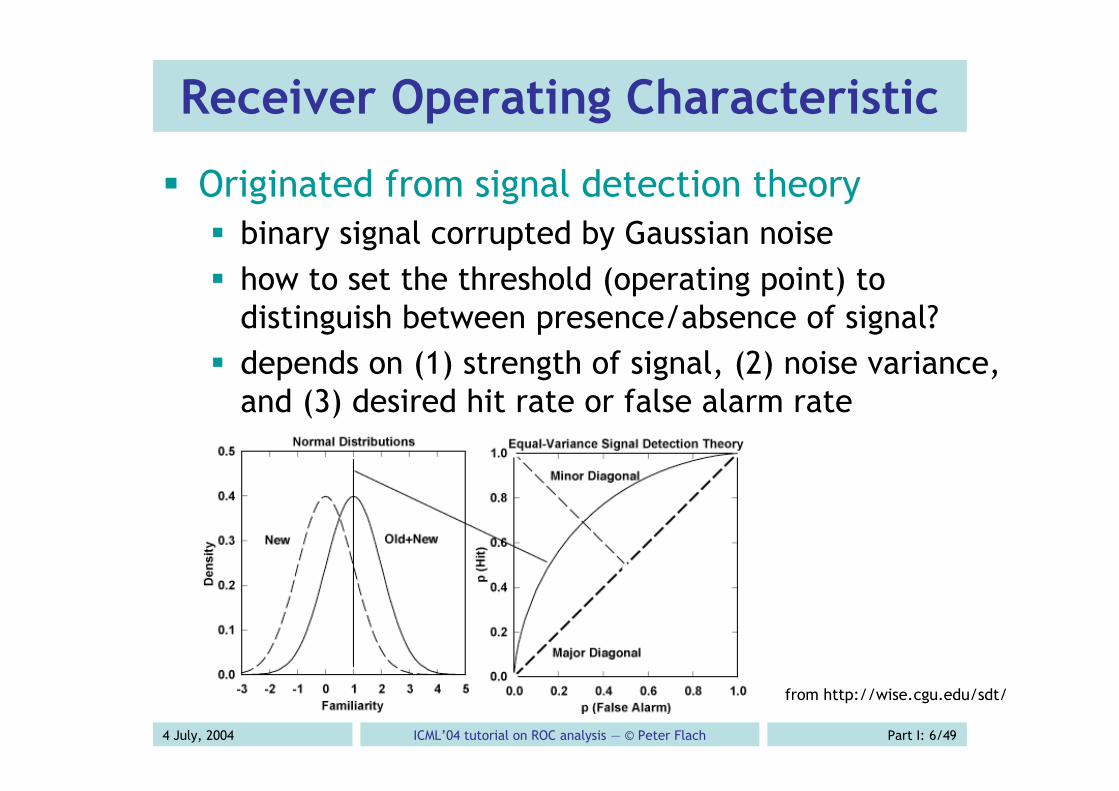
Receiver Operating Characteristic
Originated from signal detection theory binary signal corrupted by Gaussian noise how to set the threshold (operating point) to
distinguish between presence/absence of signal? depends on (1) strength of signal, (2) noise variance,
and (3) desired hit rate or false alarm rate

4 July, 2004 ICML’04 tutorial on ROC analysis — © Peter Flach Part I: 7/49
Signal detection theory
slope of ROC curve is equal to likelihood ratio
if variances are equal, L(x) increasesmonotonically with x and ROC curve is convex optimal threshold for x0 such that
concavities occur with unequal variances
€
L(x) =P(x |signal)P(x |noise)
€
L(x0) =P(noise)P(signal)

4 July, 2004 ICML’04 tutorial on ROC analysis — © Peter Flach Part I: 8/49
ROC analysis for classification
Based on contingency table or confusion matrix
Terminology: true positive = hit true negative = correct rejection false positive = false alarm (aka Type I error) false negative = miss (aka Type II error)
positive/negative refers to prediction true/false refers to correctness
Predictedpositive
Predictednegative
Positiveexamples
True positives False negatives
Negativeexamples
False positives True negatives

4 July, 2004 ICML’04 tutorial on ROC analysis — © Peter Flach Part I: 9/49
More terminology & notation
True positive rate tpr = TP/Pos = TP/TP+FN fraction of positives correctly predicted
False positive rate fpr = FP/Neg = FP/FP+TN fraction of negatives incorrectly predicted = 1 – true negative rate TN/FP+TN
Accuracy acc = pos*tpr + neg*(1–fpr) weighted average of true positive and true
negative rates
Predictedpositive
Predictednegative
Positiveexamples
TP FN Pos
Negativeexamples
FP TN Neg
PPos PNeg N

4 July, 2004 ICML’04 tutorial on ROC analysis — © Peter Flach Part I: 10/49
A closer look at ROC space
0%
20%
40%
60%
80%
100%
0% 20% 40% 60% 80% 100%
False positive rate
True
pos
itiv
e ra
te
ROC Heaven
ROC HellAlwaysNeg
AlwaysPos
A random classifier (p=0.5)
A worse than random classifier…
…can be made better than randomby inverting its predictions

4 July, 2004 ICML’04 tutorial on ROC analysis — © Peter Flach Part I: 11/49
Example ROC plot
ROC plot produced by ROCon (http://www.cs.bris.ac.uk/Research/MachineLearning/rocon/)
4 July, 2004 ICML’04 tutorial on ROC analysis — © Peter Flach Part I: 12/49
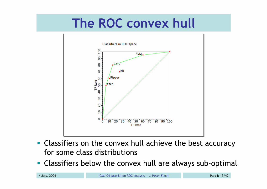
The ROC convex hull
Classifiers on the convex hull achieve the best accuracyfor some class distributions
Classifiers below the convex hull are always sub-optimal

4 July, 2004 ICML’04 tutorial on ROC analysis — © Peter Flach Part I: 13/49
Why is the convex hull a curve?
Any performance on a line segmentconnecting two ROC points can be achievedby randomly choosing between them the ascending default performance diagonal is
just a special case
The classifiers on the ROC convex hull can becombined to form the ROCCH-hybrid (Provost& Fawcett, 2001) ordered sequence of classifiers can be turned into a ranker
as with decision trees, see later

4 July, 2004 ICML’04 tutorial on ROC analysis — © Peter Flach Part I: 14/49
Iso-accuracy lines Iso-accuracy line connects ROC points with the same
accuracy pos*tpr + neg*(1–fpr) = a
Parallel ascending lineswith slope neg/pos higher lines are better on descending diagonal,
tpr = a
€
tpr =a − neg
pos+
negpos
fpr

4 July, 2004 ICML’04 tutorial on ROC analysis — © Peter Flach Part I: 15/49
Iso-accuracy & convex hull
Each line segment on the convex hull is aniso-accuracy line for a particular classdistribution under that distribution, the two classifiers on the
end-points achieve the same accuracy for distributions skewed towards negatives
(steeper slope), the left one is better for distributions skewed towards positives
(flatter slope), the right one is better
Each classifier on convex hull is optimal for aspecific range of class distributions

4 July, 2004 ICML’04 tutorial on ROC analysis — © Peter Flach Part I: 16/49
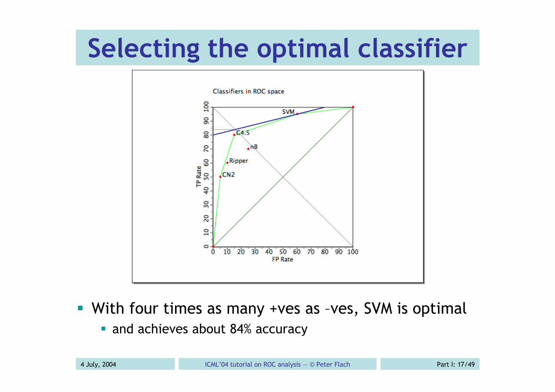
Selecting the optimal classifier
For uniform class distribution, C4.5 is optimal and achieves about 82% accuracy
4 July, 2004 ICML’04 tutorial on ROC analysis — © Peter Flach Part I: 17/49
Selecting the optimal classifier
With four times as many +ves as –ves, SVM is optimal and achieves about 84% accuracy

4 July, 2004 ICML’04 tutorial on ROC analysis — © Peter Flach Part I: 18/49
Selecting the optimal classifier
With four times as many –ves as +ves, CN2 is optimal and achieves about 86% accuracy

4 July, 2004 ICML’04 tutorial on ROC analysis — © Peter Flach Part I: 19/49
Selecting the optimal classifier
With less than 9% positives, AlwaysNeg is optimal With less than 11% negatives, AlwaysPos is optimal

4 July, 2004 ICML’04 tutorial on ROC analysis — © Peter Flach Part I: 20/49
Incorporating costs and profits
Iso-accuracy and iso-error lines are the same err = pos*(1–tpr) + neg*fpr slope of iso-error line is neg/pos
Incorporating misclassification costs: cost = pos*(1–tpr)*C(–|+) + neg*fpr*C(+|–) slope of iso-cost line is neg*C(+|–)/pos*C(–|+)
Incorporating correct classification profits: cost = pos*(1–tpr)*C(–|+) + neg*fpr*C(+|–) +
pos*tpr*C(+|+) + neg*(1–fpr)*C(–|–) slope of iso-yield line is
neg*[C(+|–)–C(–|–)]/pos*[C(–|+)–C(+|+)]

4 July, 2004 ICML’04 tutorial on ROC analysis — © Peter Flach Part I: 21/49
Skew
From a decision-making perspective, thecost matrix has one degree of freedom need full cost matrix to determine absolute yield
There is no reason to distinguish betweencost skew and class skew skew ratio expresses relative importance of
negatives vs. positives
ROC analysis deals with skew-sensitivityrather than cost-sensitivity

4 July, 2004 ICML’04 tutorial on ROC analysis — © Peter Flach Part I: 22/49
Rankers and classifiers
A scoring classifier outputs scores f(x,+)and f(x,–) for each class e.g. estimate class-conditional likelihoods
P(x|+) and P(x|–) scores don’t need to be normalised
f(x) = f(x,+)/f(x,–) can be used to rankinstances from most to least likely positive e.g. likelihood ratio P(x|+)/P(x|–)
Rankers can be turned into classifiers bysetting a threshold on f(x)

4 July, 2004 ICML’04 tutorial on ROC analysis — © Peter Flach Part I: 23/49
Drawing ROC curves for rankers
Naïve method: consider all possible thresholds
in fact, only k+1 for k instances
construct contingency table for each threshold plot in ROC space
Practical method: rank test instances on decreasing score f(x) starting in (0,0), if the next instance in the
ranking is +ve move 1/Pos up, if it is –ve move1/Neg to the right make diagonal move in case of ties

4 July, 2004 ICML’04 tutorial on ROC analysis — © Peter Flach Part I: 24/49
Some example ROC curves
Good separation between classes, convex curve

4 July, 2004 ICML’04 tutorial on ROC analysis — © Peter Flach Part I: 25/49
Some example ROC curves
Reasonable separation, mostly convex
4 July, 2004 ICML’04 tutorial on ROC analysis — © Peter Flach Part I: 26/49
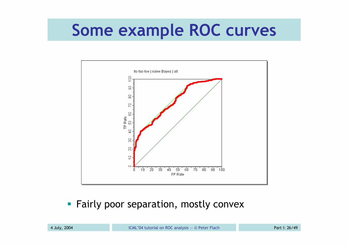
Some example ROC curves
Fairly poor separation, mostly convex

4 July, 2004 ICML’04 tutorial on ROC analysis — © Peter Flach Part I: 27/49
Some example ROC curves
Poor separation, large and small concavities

4 July, 2004 ICML’04 tutorial on ROC analysis — © Peter Flach Part I: 28/49
Some example ROC curves
Random performance

4 July, 2004 ICML’04 tutorial on ROC analysis — © Peter Flach Part I: 29/49
ROC curves for rankers
The curve visualises the quality of the rankeror probabilistic model on a test set, withoutcommitting to a classification threshold aggregates over all possible thresholds
The slope of the curve indicates classdistribution in that segment of the ranking diagonal segment -> locally random behaviour
Concavities indicate locally worse thanrandom behaviour convex hull corresponds to discretising scores can potentially do better: repairing concavities

4 July, 2004 ICML’04 tutorial on ROC analysis — © Peter Flach Part I: 30/49
The AUC metric The Area Under ROC Curve (AUC) assesses the
ranking in terms of separation of the classes all the +ves before the –ves: AUC=1 random ordering: AUC=0.5 all the –ves before the +ves: AUC=0
Equivalent to the Mann-Whitney-Wilcoxonsum of ranks test estimates probability that randomly chosen +ve is
ranked before randomly chosen –ve where S+ is the sum of ranks of +ves
Gini coefficient = 2*AUC–1 (area above diag.) NB. not the same as Gini index!
€
S+ − Pos(Pos + 1)/2Pos ⋅ Neg

4 July, 2004 ICML’04 tutorial on ROC analysis — © Peter Flach Part I: 31/49
AUC=0.5 not always random
Poor performance because data requires twoclassification boundaries

4 July, 2004 ICML’04 tutorial on ROC analysis — © Peter Flach Part I: 32/49
Turning rankers into classifiers
Requires decision rule, i.e. setting athreshold on the scores f(x) e.g. Bayesian: predict positive if equivalently:
If scores are calibrated we can use a defaultthreshold of 1 with uncalibrated scores we need to learn the
threshold from the data NB. naïve Bayes is uncalibrated
i.e. don’t use Pos/Neg as prior!
€
P(x |+) ⋅ PosP(x |−) ⋅ Neg
> 1
€
P(x |+)P(x |−)
>NegPos
4 July, 2004 ICML’04 tutorial on ROC analysis — © Peter Flach Part I: 33/49
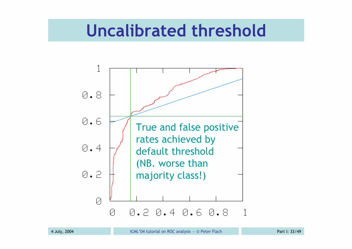
Uncalibrated threshold
True and false positiverates achieved bydefault threshold(NB. worse thanmajority class!)

4 July, 2004 ICML’04 tutorial on ROC analysis — © Peter Flach Part I: 34/49
Calibrated threshold
Optimalachievableaccuracy

4 July, 2004 ICML’04 tutorial on ROC analysis — © Peter Flach Part I: 35/49
Calibration
Easy in the two-class case: calculateaccuracy in each point/threshold whiletracing the curve, and return the thresholdwith maximum accuracy NB. only calibrates the threshold, not the
probabilities -> (Zadrozny & Elkan, 2002)
Non-trivial in the multi-class case discussed later

4 July, 2004 ICML’04 tutorial on ROC analysis — © Peter Flach Part I: 36/49
Averaging ROC curves To obtain a cross-validated ROC curve
just combine all test folds with scores for eachinstance, and draw a single ROC curve
To obtain cross-validated AUC estimate witherror bounds calculate AUC in each test fold and average or calculate AUC from single cv-ed curve and use
bootstrap resampling for error bounds
To obtain ROC curve with error bars vertical averaging (sample at fixed fpr points) threshold averaging (sample at fixed thresholds) see (Fawcett, 2004)

4 July, 2004 ICML’04 tutorial on ROC analysis — © Peter Flach Part I: 37/49
Averaging ROC curves
From (Fawcett, 2004)
(a) ROC curves from five test samples (b) ROC curve from combining the samples
(c) Vertical averaging, fixing fpr (d) Threshold averaging

4 July, 2004 ICML’04 tutorial on ROC analysis — © Peter Flach Part I: 38/49
PN spaces PN spaces are ROC spaces with non-
normalised axes x-axis: covered –ves n (instead of fpr = n/Neg) y-axis: covered +ves p (instead of tpr = p/Pos)

4 July, 2004 ICML’04 tutorial on ROC analysis — © Peter Flach Part I: 39/49
PN spaces vs. ROC spaces
PN spaces can be used if class distribution(reflected by shape) is fixed good for analysing behaviour of learning
algorithm on single dataset (Gamberger & Lavrac,2002; Fürnkranz & Flach, 2003)
In PN spaces, iso-accuracylines always have slope 1 PN spaces can be nested
to reflect covering strategy

4 July, 2004 ICML’04 tutorial on ROC analysis — © Peter Flach Part I: 40/49
Precision-recall curves
Precision prec = TP/PPos = TP/TP+FP fraction of positive predictions correct
Recall rec = tpr = TP/Pos = TP/TP+FN fraction of positives correctly predicted
Note: neither depends on true negatives makes sense in information retrieval, where true
negatives tend to dominate —> low fpr easy
Predictedpositive
Predictednegative
Positiveexamples
TP FN Pos
Negativeexamples
FP TN Neg
PPos PNeg N

4 July, 2004 ICML’04 tutorial on ROC analysis — © Peter Flach Part I: 41/49
From (Fawcett, 2004)
PR curves vs. ROC curves
Two ROC curves Corresponding PR curves
→ Recall
→ P
reci
sion

4 July, 2004 ICML’04 tutorial on ROC analysis — © Peter Flach Part I: 42/49
DET curves (Martin et al., 1997)
Detection Error Trade-off false negative rate instead of true positive rate re-scaling using normal deviate scale
.1 .2 .5 1 2 5 10 20 40
.1 .2
.5 1 2
5
10
20
40
False Alarm Probability (in %)
Miss Probability (in %)
Minimum Cost point
0 0.1 0.2 0.3 0.4 0.50.5
0.6
0.7
0.8
0.9
1
False Alarm Probability (in %)
Correct Detection (in %)
Minimum Cost point

4 July, 2004 ICML’04 tutorial on ROC analysis — © Peter Flach Part I: 43/49
Erro
r ra
te
Probability of +ves pos0.8 1.00.0 0.2 0.4 0.6
0.0
0.2
0.4
0.6
0.8
1.0Classifier 1tpr = 0.4fpr = 0.3
Classifier 2tpr = 0.7fpr = 0.5
Classifier 3tpr = 0.6fpr = 0.2
fpr 1-tpr
Cost curves (Drummond & Holte, 2001)

4 July, 2004 ICML’04 tutorial on ROC analysis — © Peter Flach Part I: 44/49
Erro
r ra
te
Probability of +ves pos0.8 1.00.0 0.2 0.4 0.6
0.0
0.2
0.4
0.6
0.8
1.0
AlwaysNegAlwaysPos
Operating range
Operating range

4 July, 2004 ICML’04 tutorial on ROC analysis — © Peter Flach Part I: 45/49
Erro
r ra
te
Probability of +ves pos0.8 1.00.0 0.2 0.4 0.6
0.0
0.2
0.4
0.6
0.8
1.0
Lower envelope

4 July, 2004 ICML’04 tutorial on ROC analysis — © Peter Flach Part I: 46/49
Erro
r ra
te
Probability of +ves pos0.8 1.00.0 0.2 0.4 0.6
0.0
0.2
0.4
0.6
0.8
1.0
Varying thresholds
AlwaysNegAlwaysPos

4 July, 2004 ICML’04 tutorial on ROC analysis — © Peter Flach Part I: 47/49
Taking costs into account
Error rate is err = (1–tpr)*pos + fpr*(1–pos)
Define probability cost function as
Normalised expected cost is nec = (1–tpr)*pcf + fpr*(1–pcf)
€
pcf =pos ⋅C(−|+)
pos ⋅C(−|+)+ neg ⋅C(+|−)

4 July, 2004 ICML’04 tutorial on ROC analysis — © Peter Flach Part I: 48/49
Operating rangesurprisingly narrow
Performanceonly so-so
ROC curve vs. cost curve

4 July, 2004 ICML’04 tutorial on ROC analysis — © Peter Flach Part I: 49/49
Summary of Part I
ROC analysis is useful for evaluatingperformance of classifiers and rankers key idea: separate performance on classes
ROC curves contain a wealth of informationfor understanding and improvingperformance of classifiers requires visual inspection