1

The Main Factors Affecting Heat Transfer Along Dense Phase CO2 Pipelines 1

B. Wetenhall1*, J.M. Race2, H. Aghajani1 and J. Barnett3 2 1 School of Marine Science and Technology, Newcastle University, Newcastle, NE17RU, UK 3

2 Department of Naval Architecture, Ocean and Marine Engineering, University of Strathclyde, 4

Glasgow, G4 0LZ, UK 5 3 National Grid, 35 Homer Road, Solihull, West Midlands, B91 3QJ, UK 6

7

ABSTRACT 8

Carbon Capture and Storage (CCS) schemes will necessarily involve the transportation of large 9

volumes of carbon dioxide (CO2) from the capture source of the CO2 to the storage or utilisation site. 10

It is likely that the majority of the onshore transportation of CO2 will be through buried pipelines. 11

Although onshore CO2 pipelines have been operational in the United States of America for over 40 12

years, the design of CO2 pipelines for CCS systems still presents some challenges when compared 13

with the design of natural gas pipelines. The aim of this paper is to investigate the phenomenon of 14

heat transfer from a buried CO2 pipeline to the surrounding soil and to identify the key parameters 15

that influence the resultant soil temperature. It is demonstrated that, unlike natural gas pipelines, the 16

CO2 in the pipeline retains its heat for longer distances resulting in the potential to increase the 17

ambient soil temperature and influence environmental factors such as crop germination and water 18

content. The parameters that have the greatest effect on heat transfer are shown to be the inlet 19

temperature and flow rate, i.e. pipeline design parameters which can be dictated by the capture plant 20

and pipeline’s design and operation rather than environmental parameters. Consequently, by carefully 21

controlling the design parameters of the pipeline it is possible to control the heat transfer to the soil 22

and the temperature drop along the pipeline. 23

24

KEYWORDS 25

CO2 pipelines, temperature profile, sensitivity analysis, heat transfer, soil temperature, hydraulic 26

modelling, CCS 27

28 29

1. INTRODUCTION 30

Carbon Capture and Storage (CCS) is one method of reducing carbon dioxide (CO2) emissions into 31

the atmosphere which would otherwise contribute towards global climate change. CCS involves 32

capturing CO2 from a large industrial point source (such as a power station) and transporting the CO2 33

for either usage (for example for Enhanced Oil Recovery (EOR)) or for permanent storage in a 34

* Corresponding author: Tel: (0044) 191 2085532 ; E-mail: ben.wetenhall@ncl.ac.uk

2

geological site. Depending on the distance and availability of a suitable storage site, the transportation 35

of the CO2 to the storage site is by means of a pipeline network, by ship based transportation or a 36

combination of both. 37

38

For the onshore pipeline transportation of CO2, after compression at the capture plant, the CO2 39

streams will typically be at temperatures between 30°C to 50°C and pressures between 10MPa to 20 40

MPa (Farris, 1983; Race et al., 2012) putting the CO2 streams in either supercritical or dense phase. 41

For CO2 pipelines, it is important to understand how the temperature of the fluid varies along the 42

pipeline, as the temperature determines the phase of the fluid and affects density, pressure drop 43

(Dongjie et al., 2012) and economics (Teh et al., 2015; Zhang et al., 2006). Colder ground conditions 44

provide greater cooling of the CO2 stream and, as a result, lower inlet pressures are required to keep 45

the CO2 in a liquid phase. In addition, higher densities are maintained at lower temperatures, which is 46

more efficient for pipeline transportation and better for pump operation. 47

48

When the fluid temperature is higher than that of the surrounding soil, due to the temperature 49

difference between the CO2 and surroundings and elevation changes along the pipeline route, there 50

will be heat exchange between the CO2 stream and the surrounding environment with the temperature 51

of the fluid getting closer to (but not necessarily reaching) ambient temperature along the length of the 52

pipeline. The heat transfer between the fluid and the surrounding soil takes place in 4 stages: firstly 53

there is forced convection from the film of fluid coating the inner surface of the pipeline, the second 54

stage of heat transfer is conduction through the pipe wall, heat transfer then proceeds via conduction 55

from the outer surface of the pipeline and through the surrounding soil. Finally there is natural 56

convection from the surface of the soil to the surrounding air. In the conduction stages through the 57

pipeline and from the pipeline to the soil, it is possible to include the effects of any pipeline coatings 58

(which may be included on the pipe internal surface, for example to, facilitate flow) and insulation on 59

the outside of the pipe. In this work coatings are neglected due to a lack of publically available 60

information on their heat transfer properties and no insulation is added to the pipeline following the 61

planned demonstration projects in the UK (Capture Power, 2016). 62

63

In natural gas pipelines the fluid generally reaches ambient temperature very rapidly but in CO2 64

pipelines this process can be much slower. Heat transfer from the fluid to the surroundings can cause 65

environmental issues. For example, pipelines carrying warm fluid can cause heating of the 66

surrounding soil, which may result in premature crop growth and affect soil moisture and the 67

temperature along the pipeline Right of Way (ROW) (Dunn et al., 2008; Naeth et al., 1993; Neilsen et 68

al., 1990) in some circumstances. In order for a pipeline operator to be able to manage these effects, it 69

is important to understand the degree of influence that operational and environmental factors have on 70

heat flux from the fluid to the surrounding soil. Factors influencing the degree of heat flux from a 71

3

buried pipeline include the fluid pressure and temperature, the soil temperature, the soil type and 72

moisture content (Becker et al., 1992), the thermal conductivity of the pipeline steel and the elevation 73

profile along the pipeline route (Teh et al., 2015). Some parameters such as the temperature of the 74

fluid, operating pressure and initial temperature of the CO2 can be controlled at the capture plant. 75

Other parameters, such as the soil type and ambient temperature are out of the control of the pipeline 76

operator. 77

78

1.1. Heat transfer from CO2 pipelines 79

There is very little publically available work on heat transfer from CO2 pipelines. The heat transfer 80

characteristics of CO2 pipelines surrounded by water were analysed experimentally and 81

computationally by Drescher et al. (2013). They found that the water temperature has a high impact 82

on the amount of heat transfer and a range of values for the overall heat transfer coefficient for a CO2 83

pipelines surrounded by water, finding a mean value of 44.7W/m2K. The importance to CO2 pipeline 84

operation of the soil temperature and type, thermal conductivity of the pipeline and topography of the 85

pipeline route was highlighted in Dongjie et al. (2012) and Teh et al. (2015). They found that 86

transporting and storing liquid CO2 can be cheaper than supercrtical CO2, that cooler ground 87

conditions can lead to cost savings and highlighted the need for futher work to explore the effect of 88

burial depth and of soil thermal conductivity. The effect of pipeline operating temperature on UK 89

soils was investigated in Lake et al. (2016) who provided the first set of empirical data on soil 90

temperature and moisture profiles for CCS pipelines. There is still need for further work on how best 91

to operate a CO2 pipeline with regards to heat transfer and experimental work into heat transfer from 92

full scale CO2 pipelines. This work is a step towards the former. 93

94

Through pipeline simulations and a sensitivity analysis this study identifies the dominant parameters 95

affecting heat transfer from liquid CO2 pipelines and discusses how an operator can control heat 96

transfer out of the pipeline to minimise the impact of heat transfer. Firstly a preliminary study was 97

conducted consisting of a series of eight steady-state pipeline simulations. This allowed an 98

investigation of the influence of ground temperature, flow rate, inlet temperature, burial depth, soil 99

conductivity, inlet pressure and CO2 composition on the rate of temperature loss along the pipeline 100

and a comparison to previous results. A sensitivity analysis, using a Gaussian emulator, was then 101

performed to identify which of the parameters investigated in the preliminary analysis had the 102

strongest influence on the temperature drop along the pipeline. The Gaussian emulation approach is 103

highly computationally efficient (far fewer model runs are required compared with, for example, 104

Monte-Carlo based methods), it allows for a complete range of sensitivity measures to be computed 105

from one set of pipeline simulation results and statistical performance is included in the process. It is 106

applicable to the current study because the data from the pipeline simulations is smooth (i.e. there are 107

4

no sudden jumps when moving between data points). Smoothness was ensured by keeping the 108

pipeline simulations in the dense or supercritical phase. 109

110

2. HYDRAULIC MODELLING OF THE CO2 PIPELINES 111

2.1. Model setup 112

The modelling approach that was adopted for this study is described in detail in (Wetenhall et al., 113

2014). Heat transfer modelling details are given in Section 2.2 while the other details are presented in 114

summary. PIPESIM, a steady-state flow simulator (Schlumberger, 2010), was used to conduct the 115

hydraulic modelling of the CO2 pipeline. As implemented in the software package MultiFlash 116

(Infochem, 2011), the fluid physical (density, enthalpy, compressibility and heat capacity) and phase 117

properties were determined using the Peng-Robinson Equation of State (Peng and Robinson, 1976), 118

fluid viscosity was calculated using the Pedersen model (Pedersen et al., 1984) and SUPERTRAPP 119

(NIST, 2007) was used to determine fluid thermal conductivity. Figure 1 shows a flow diagram for 120

the pipeline simulation procedure as implemented in PIPESIM. The procedure requires the 121

simultaneous solution of the conservation of mass, momentum and energy equations. From the 122

solution of these equations, the pressure and temperature drops along the length of the pipeline can be 123

calculated given two of the parameters of initial pressure, final pressure or flow rate. It is recognised 124

that the Pedersen model was developed for oil applications but it has been shown to provide a 125

conservative prediction for the hydraulic modelling of CO2 streams in the absence of a CO2 viscosity 126

model (Wetenhall et al., 2014). The flow equation selected for this analysis was the Beggs and Brill 127

correlation (Beggs and Brill, 1973) with the Moody friction factor (Moody, 1944) as defined in Brill 128

and Mukherjee (1999). 129

130

2.2. Modelling the heat transfer from the fluid to the surrounding soil 131

To calculate the rate of heat transfer from the fluid contained inside the pipeline to the surrounding 132

soil, the pipeline is first divided into segments. The maximum segment length was set to 0.05m, as it 133

was found that the results were not sensitive to smaller segmentation lengths. For each segment, a 134

heat transfer balance is performed using the First Law of Thermodynamics, i.e. the total amount of 135

energy entering the pipeline segment must equal the amount of energy leaving the segment plus the 136

energy transferred to or from the surroundings. The hydraulic modelling procedure couples the 137

change in fluid properties with the heat and work done to the fluid through the pipeline segment. 138

139

For steady state flow, the First Law of Thermodynamics for a pipeline segment may be written as 140

(Mohitpour et al., 2003): 141

Δ ��𝐻 +12𝑣𝑚2 + 𝑔𝑔�𝑑𝑑� = Σ𝛿𝛿 − 𝛿𝛿 (1)

142

5

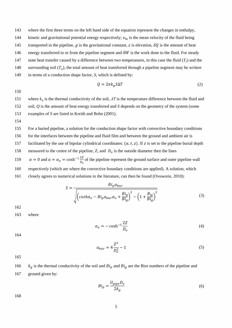
where the first three terms on the left hand side of the equation represent the changes in enthalpy, 143

kinetic and gravitational potential energy respectively; 𝑣𝑚 is the mean velocity of the fluid being 144

transported in the pipeline, 𝑔 is the gravitational constant, 𝑔 is elevation, 𝛿𝛿 is the amount of heat 145

energy transferred to or from the pipeline segment and 𝛿𝛿 is the work done to the fluid. For steady 146

state heat transfer caused by a difference between two temperatures, in this case the fluid (Tf) and the 147

surrounding soil (Tg), the total amount of heat transferred through a pipeline segment may be written 148

in terms of a conduction shape factor, S, which is defined by: 149

𝛿 = 2𝜋𝑘𝑔𝑆Δ𝑇 (2) 150

where kg is the thermal conductivity of the soil, ΔT is the temperature difference between the fluid and 151

soil, Q is the amount of heat energy transferred and S depends on the geometry of the system (some 152

examples of S are listed in Kreith and Bohn (2001). 153

154

For a buried pipeline, a solution for the conduction shape factor with convective boundary conditions 155

for the interfaces between the pipeline and fluid film and between the ground and ambient air is 156

facilitated by the use of bipolar cylindrical coordinates: (𝛼, 𝜏, 𝑔). If 𝑔 is set to the pipeline burial depth 157

measured to the centre of the pipeline, Z, and 𝐷𝑜 is the outside diameter then the lines 158

𝛼 = 0 and 𝑎 = 𝛼𝑜 = cosh−1 2𝑍𝐷𝑜

of the pipeline represent the ground surface and outer pipeline wall 159

respectively (which are where the convective boundary conditions are applied). A solution, which 160

closely agrees to numerical solutions in the literature, can then be found (Ovuworie, 2010): 161

𝑆 =𝐵𝑖𝑝𝑎𝑏𝑏𝑏

��𝑐𝑐𝑐ℎ𝛼𝑜 − 𝐵𝑖𝑝𝑎𝑏𝑏𝑏𝛼𝑜 +𝐵𝑖𝑝𝐵𝑖𝑔

�2− �1 +

𝐵𝑖𝑝𝐵𝑖𝑔

�2

(3)

162

where 163

𝛼𝑜 = − cosh−12𝑍𝐷𝑜

(4)

164

𝑎𝑏𝑏𝑏 = 4𝑍2

𝐷𝑜2− 1 (5)

165

𝑘𝑔 is the thermal conductivity of the soil and 𝐵𝑖𝑝 and 𝐵𝑖𝑔 are the Biot numbers of the pipeline and 166

ground given by: 167

𝐵𝑖𝑝 =𝑈𝑝𝑖𝑝𝑝𝐷𝑜

2𝑘𝑔 (6)

168

6

𝐵𝑖𝑔 =ℎ𝑎𝐷𝑜2𝑘𝑔

(7)

169

Here, ℎ𝑎 is the heat transfer coefficient of the fluid film of ambient air at the ground surface and the 170

overall heat transfer coefficient of the pipeline, Upipe, is a combination of the heat transfer coefficients 171

of the fluid film, hfilm, and pipeline, hpipe: 172

1𝑈𝑝𝑖𝑝𝑝

=1

ℎ𝑓𝑖𝑓𝑚+

1ℎ𝑝𝑖𝑝𝑝

(8)

173

The heat transfer coefficients of the pipeline and the films of fluid between the pipeline and internal 174

fluid and the ambient air and soil can be determined by considering the layers between the fluid and 175

pipeline wall (convective) and radially outwards through the pipeline wall (conductive) separately. 176

177

2.2.1. Heat transfer between the ambient air and surface of the soil 178

Heat transfer from the surface of the soil to the film of ambient air at the surface is convective and the 179

corresponding heat transfer coefficient may be split into a free convection component, ℎ𝑓𝑏𝑝𝑝, 180

(capturing the density differences) and a forced convection component, ℎ𝑓𝑜𝑏𝑓𝑝𝑓, (capturing the effect 181

of the wind): 182

ℎ𝑎 = ℎ𝑓𝑜𝑏𝑓𝑝𝑓 + ℎ𝑓𝑏𝑝𝑝 (9)

183

As the wind speed is below 0.5m/s close to the soil surface, the free convection component dominates 184

so a limiting value of 4W/m2K was used for ha (Schlumberger, 2010). 185

186

2.2.2. Heat transfer between the fluid film and pipeline wall 187

Heat transfer from the film of fluid at the surface of the pipeline to the inner pipeline wall is 188

convective and the heat transfer coefficient for this layer may be expressed as: 189

ℎ𝑓𝑖𝑓𝑚 =𝑘𝑓𝑁𝑁𝐷𝑖

(10)

where 𝑘𝑓 is the thermal conductivity of the fluid (calculated using SUPERTRAPP (NIST, 2007)), Nu 190

is the Nusselt number and 𝐷𝑖 is the pipeline inner diameter. For the flow conditions considered in this 191

study, the flow regime is always seen to be turbulent (with Reynold’s numbers of the order 106), and 192

therefore, for the Nusselt number, semi-empirical correlations of the Reynold’s number and Prandtl 193

number can be used (Kreith and Bohn, 2001): 194

𝑁𝑁 = 0.023𝑅𝑒0.8𝑃𝑃0.33 �1 + �𝐷𝑖𝛿𝛿�� (11)

7

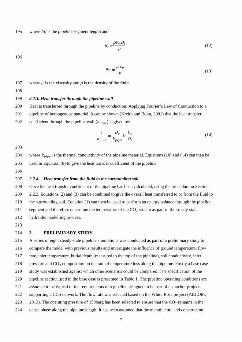
where 𝛿𝛿 is the pipeline segment length and 195

Re=ρ𝑣𝑚𝐷𝑖µ (12)

196

𝑃𝑃 =𝜇 𝑐𝑝𝑘

(13)

where µ is the viscosity and ρ is the density of the fluid. 197

198

2.2.3. Heat transfer through the pipeline wall 199

Heat is transferred through the pipeline by conduction. Applying Fourier’s Law of Conduction to a 200

pipeline of homogenous material, it can be shown (Kreith and Bohn, 2001) that the heat transfer 201

coefficient through the pipeline wall (ℎ𝑝𝑖𝑝𝑝) is given by: 202

1ℎ𝑝𝑖𝑝𝑝

=𝐷𝑜𝑘𝑝𝑖𝑝𝑝

ln𝐷𝑜𝐷𝑖

(14)

203

where 𝑘𝑝𝑖𝑝𝑝 is the thermal conductivity of the pipeline material. Equations (10) and (14) can then be 204

used in Equation (8) to give the heat transfer coefficient of the pipeline. 205

206

2.2.4. Heat transfer from the fluid to the surrounding soil 207

Once the heat transfer coefficient of the pipeline has been calculated, using the procedure in Section 208

2.2.3, Equations (2) and (3) can be combined to give the overall heat transferred to or from the fluid to 209

the surrounding soil. Equation (1) can then be used to perform an energy balance through the pipeline 210

segment and therefore determine the temperature of the CO2 stream as part of the steady-state 211

hydraulic modelling process. 212

213

3. PRELIMINARY STUDY 214

A series of eight steady-state pipeline simulations was conducted as part of a preliminary study to 215

compare the model with previous results and investigate the influence of ground temperature, flow 216

rate, inlet temperature, burial depth (measured to the top of the pipeline), soil conductivity, inlet 217

pressure and CO2 composition on the rate of temperature loss along the pipeline. Firstly a base case 218

study was established against which other scenarios could be compared. The specification of the 219

pipeline section used in the base case is presented in Table 1. The pipeline operating conditions are 220

assumed to be typical of the requirements of a pipeline designed to be part of an anchor project 221

supporting a CCS network. The flow rate was selected based on the White Rose project (AECOM, 222

2013). The operating pressure of 150barg has been selected to ensure that the CO2 remains in the 223

dense phase along the pipeline length. It has been assumed that the manufacture and construction 224

8

standards and practices for CO2 pipelines will be similar to those used for natural gas pipelines and 225

therefore no insulation has been applied to the pipelines in the hydraulic model and the pipes have 226

been buried to a depth of 1.2m as measured from the top of the pipeline. This figure is considered to 227

be representative of the maximum depth of cover required for the construction of onshore pipelines in 228

the UK (PD8010-1, 2015). A roughness value of 0.0457mm has been used as the recommended value 229

for commercial steel pipelines (Mohitpour et al., 2003). The soil thermal conductivity is considered to 230

be constant along the length of the pipeline and has been taken to be 0.87W/mK, which is typical of a 231

moist sandy or clay type soil (McAllister, 2005). The ambient ground temperature has been set at 3oC 232

for the base case representing a winter scenario in the UK. 233

234

Having established this base case pipeline, seven cases were run to investigate the influence of ground 235

temperature, flow rate, inlet temperature, burial depth, soil conductivity, inlet pressure and CO2 236

composition on the rate of temperature and pressure loss along the pipeline. The parameters that were 237

changed for each study from the base case are detailed in Table 2. Of particular note is the approach 238

taken to investigate the effect of composition. Previous work indicates that the influence of a 239

particular component in hydraulic analysis is highly influenced by the critical temperature and 240

pressure of the component or impurity relative to pure CO2 (Race et al., 2012; Wetenhall et al., 2014). 241

In this respect, the two impurities that could be present from power plant capture plant, which have 242

the most divergent effects on hydraulic behaviour are sulphur dioxide (SO2) and hydrogen (H2). As a 243

result only these two components have been selected to represent a best and worst case. 244

245

3.1. Preliminary study results 246

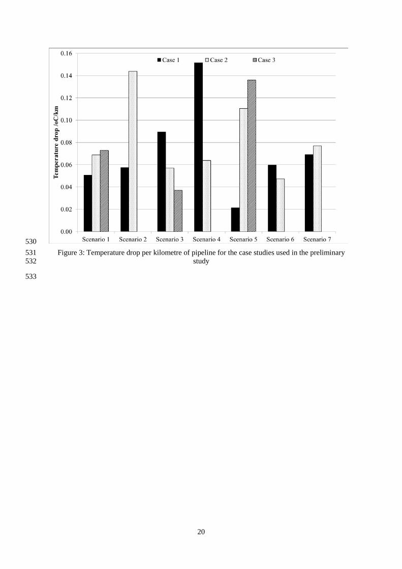
For each case listed in Table 2, the pressure and temperature profiles along the 150km long pipeline 247

were determined. The results were then presented in terms of the pressure drop/km (barg/km) or 248

temperature drop/km (oC/km) and are shown in Figure 2 and Figure 3. The pressure and temperature 249

drops per km obtained in this study are in line with the current literature (Teh et al., 2015; Zhang et 250

al., 2006)). In particular, (Teh et al., 2015) reports temperature drops of 0.04 to 0.05oC/km for 251

scenarios with similarity to Case 1.1 and (Zhang et al., 2006) reports pressure drops of 0.02 to 252

0.03bara/km for scenarios with similarity to Cases 1.1 and 3.1. 253

254

The maximum pressure drop observed was 0.05barg/km for Case 2.1, the scenario with a flow rate of 255

17MT/year and a ground temperature of 3oC. This is below pressure gradients quoted in the literature 256

for CO2 pipelines which are around 0.2bar/km (Seevam et al., 2010; Vandeginste and Piessens, 2008). 257

It is therefore concluded that the pressure drop is not significantly affected by the input parameters. 258

259

In terms of temperature drop, the temperature of the fluid does not reach the temperature of the 260

surrounding soil along the length of the pipeline. A review of the temperature profiles in Figure 3 261

9

indicates that the inlet temperature, flow rate, burial depth and soil conductivity appear to have the 262

largest effects on temperature drop. Parameters which seem to have a lesser effect are ground 263

temperature and composition. However, it is recognised that these conclusions are drawn from a small 264

sample set and the interactions between parameters have not been studied in detail in this preliminary 265

analysis. 266

4. SENSITIVITY ANALYSIS 267

The next stage in the analysis was to conduct a sensitivity analysis using a Gaussian emulator 268

approach to identify which of the parameters investigated in the preliminary analysis had the strongest 269

influence on the temperature drop along the pipeline. The rationale behind this analysis was to 270

determine the operational parameters that could or should be controlled by a pipeline operator to 271

maximise temperature drop or whether the critical parameters were environmental in nature and 272

therefore more difficult or impossible to control. 273

274

4.1. Gaussian emulator approach 275

The technique that has been used for the sensitivity analysis is the Gaussian emulator approach using 276

the Gaussian Emulation Machine for Sensitivity Analysis (GEM-SA) software (GEM-SA, 2013) 277

which provides a statistical approximation with which it is possible to perform a sensitivity analysis. 278

279

In order to perform an accurate sensitivity analysis on a model with a number of interrelated inputs (in 280

this case ground temperature, flow rate, inlet temperature, burial depth, soil conductivity and inlet 281

pressure) and outputs (temperature drop), a large number of simulation model runs is required. 282

Running this number of models in PIPESIM is prohibitive in terms of time and computer resource 283

requirements. A Gaussian emulator takes a series of inputs and the corresponding series of outputs 284

from running the simulation model (PIPESIM) and creates an emulator of the simulator, from which 285

predictive runs can be made quickly and cheaply in terms of computer processing requirements. The 286

Gaussian emulator also gives a probability distribution to show how the simulator performs away 287

from the design points. If the emulator is able to approximate the results of the simulator accurately, 288

then a sensitivity analysis of the model using the emulator is an accurate approximation to the 289

sensitivity analysis of the simulator. 290

291

4.2. Input for the Gaussian emulator 292

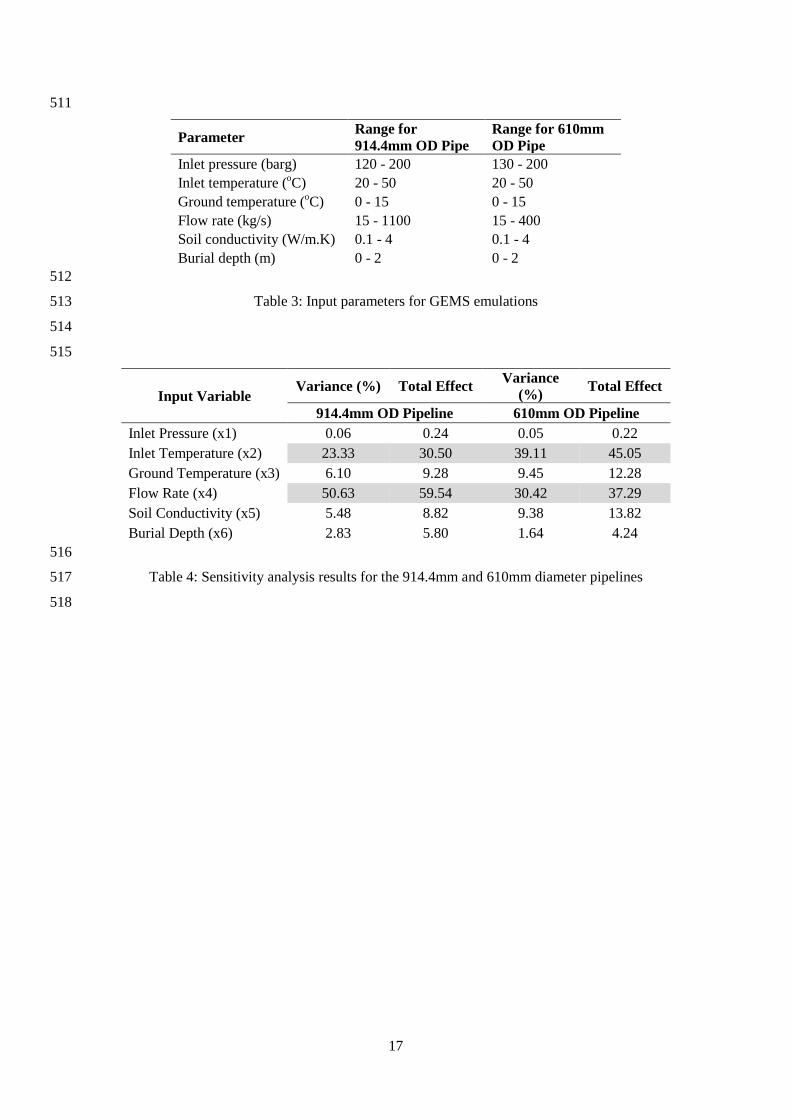
The range of input data that was used for the Gaussian Emulator is shown in Table 3. The ranges were 293

selected such that operation is maintained at pressures above the bubble point curve in order to avoid 294

two-phase flow. For the sensitivity analysis, two simulations were conducted; one for the 914.4mm 295

Outside Diameter (OD) pipeline as specified in Table 1 and the other for a 610mm OD, 19.1mm wall 296

thickness pipeline. A 610mm OD pipeline was selected as this was the size of the pipeline proposed 297

for the White Rose project (AECOM, 2013), an example of a CO2 pipeline designed to facilitate 298

10

development of a pipeline transportation network. The length of the 610mm OD pipeline and the pipe 299

roughness used in the simulation remained the same as detailed in Table 1. 300

301

A series of 200 datasets of training inputs for the Gaussian Emulator were generated using a maximin 302

Latin hypercube design1. This ensures that a good sample set of inputs was selected with which to 303

build the emulator that covers the whole parameter set range. The range is shown in Table 3. Each of 304

the 200 datasets was run in PIPESIM to obtain the training outputs. The emulator was then built using 305

the GEM-SA approach (O'Hagan, 2004). 306

307

The emulator provides a statistical approximation indicating the likelihood that the predicted value is 308

the true output of the model, i.e. in this case the PIPESIM output. At the training points, the 309

uncertainty of not emulating the simulated value is zero; away from the training outputs the 310

distribution associated with the inputs gives a mean value for the output for a Gaussian process of 311

uncertainty around the mean, each of the six input variables having a normal distribution. 312

313

4.3. Gaussian emulator results 314

The Gaussian emulators provided a good predictor for the output from PIPESIM. The variance of 315

expected code outputs for the 914.4mm and 610mm OD pipelines were 0.003 and 0.005 respectively. 316

Furthermore, predictions of the emulators were made for five sets of randomly selected model inputs 317

and compared with the corresponding output from PIPESIM. Considering the difference between the 318

predictions and PIPESIM output both emulators had 𝑅2values of 1.00. 319

320

The results of the GEM-SA emulations for the 914.4mm and 610mm OD pipelines, using the input 321

parameter ranges given in Table 3 are plotted in Figure 4 and Figure 5 respectively. The magnitude of 322

the effect on the y-axis of each graph indicates the expected value of the temperature decrease of the 323

fluid obtained by averaging over all other inputs. Negative slopes on the graphs indicate that the effect 324

on heat transfer from the fluid to the soil decreases with increasing values of the input parameter, i.e. 325

the outlet temperature of the fluid will be higher with increasing values of the input parameter. 326

Similarly, a positive slope indicates that the effect on temperature decrease of the fluid increases with 327

increasing values of the input parameter, i.e. the outlet temperature of the fluid is lower with 328

increasing values of the input parameter. The plots also indicate the uncertainty in the emulated 329

results with the wider bands indicating more uncertain regions of the emulation. Full details of the 330

theory behind the sensitivity analysis are provided in Oakley and O’Hagan, 2004). 331

332

1 Latin hypercube sampling is a statistical methodology for generating a sample of parameter values from a multi-dimensional distribution.

The sampled variables are then randomly combined into plausible variable sets for one calculation of the output function (in this case outlet temperature).

11

It is noted that the effect of the input variables on the temperature loss show the same qualitative 333

behaviour between the two pipeline diameters. However, the magnitudes of the effects are slightly 334

different for each case as a change in pipeline diameter results in a change in the pressure gradient 335

along the pipeline and therefore the results cannot be compared quantitatively. 336

337

4.3.1. Effect of input variables 338

Figure 4a and Figure 5a illustrate the effect of varying inlet pressure on the outlet temperature. Over 339

the range of pressures investigated, it can be seen that changing the inlet pressure has very little effect 340

on the outlet temperature of the fluid, provided that the inlet pressure is high enough to avoid two 341

phase flow along the entire pipeline length. The input parameters were specifically selected for the 342

GEMS emulations to avoid two-phase flow. 343

344

The effect of varying inlet temperature of the fluid is shown in Figure 4b and Figure 5b and follows a 345

linear trend as you would expect from looking at Equation (2). With increasing inlet temperatures, the 346

heat transfer from the fluid to the soil is increased and therefore the outlet temperature of the fluid is 347

decreased. However, increasing the ground temperature has a linearly decreasing effect on heat 348

transfer from the fluid (Figure 4d and Figure 5d), i.e. increasing the ground temperature decreases the 349

effect on the outlet temperature of the fluid. The same trend is shown for increasing burial depth 350

(Figure 4e and Figure 5e) although the effect tends to an asymptotic value; indicating that above about 351

1m, the burial depth has little effect on the outlet temperature of the fluid. 352

353

Soil conductivity also shows asymptotic rather than a linear behaviour with higher soil conductivities 354

increasing the amount of heat transfer from the fluid and decreasing its outlet temperature (see Figure 355

4c and Figure 5c). However the effect is less marked above a soil conductivity of about 2.5W/mK. 356

357

As the graphs of Figure 4f and Figure 5f illustrate, flow rate has a significant effect on outlet 358

temperature. As the flow rate increases less heat is transferred from the fluid to the surrounding soil 359

and therefore the fluid outlet temperature is increased. Smaller flow rates will lead to lower fluid 360

velocities and thus increased heat transfer. However, it can be seen that the largest effects occur at 361

lower flow rates with asymptotic behaviour observed at higher flow rates. For example, for the 362

914.4mm OD pipeline, increasing the flow rate above 600kg/s will have a marginal effect on the 363

outlet temperature for the simulations conducted. 364

365

At high flow rates, the pressure drops more rapidly along the pipeline than at lower flow rates. 366

Consequently, the density of the fluid decreases along the pipeline and the velocity and the Reynolds 367

Number (Re) increases. Most of the heat loss in turbulent flow is convective, as opposed to 368

conductive, and an increase in velocity causes an increase in turbulence and an increase in convective 369

12

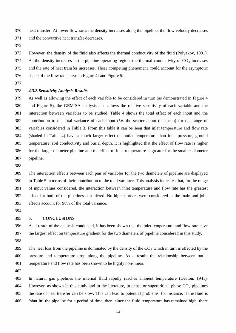
heat transfer. At lower flow rates the density increases along the pipeline, the flow velocity decreases 370

and the convective heat transfer decreases. 371

372

However, the density of the fluid also affects the thermal conductivity of the fluid (Polyakov, 1991). 373

As the density increases in the pipeline operating region, the thermal conductivity of CO2 increases 374

and the rate of heat transfer increases. These competing phenomena could account for the asymptotic 375

shape of the flow rate curve in Figure 4f and Figure 5f. 376

377

4.3.2. Sensitivity Analysis Results 378

As well as allowing the effect of each variable to be considered in turn (as demonstrated in Figure 4 379

and Figure 5), the GEM-SA analysis also allows the relative sensitivity of each variable and the 380

interaction between variables to be studied. Table 4 shows the total effect of each input and the 381

contribution to the total variance of each input (i.e. the scatter about the mean) for the range of 382

variables considered in Table 3. From this table it can be seen that inlet temperature and flow rate 383

(shaded in Table 4) have a much larger effect on outlet temperature than inlet pressure, ground 384

temperature, soil conductivity and burial depth. It is highlighted that the effect of flow rate is higher 385

for the larger diameter pipeline and the effect of inlet temperature is greater for the smaller diameter 386

pipeline. 387

388

The interaction effects between each pair of variables for the two diameters of pipeline are displayed 389

in Table 5 in terms of their contribution to the total variance. This analysis indicates that, for the range 390

of input values considered, the interaction between inlet temperature and flow rate has the greatest 391

effect for both of the pipelines considered. No higher orders were considered as the main and joint 392

effects account for 98% of the total variance. 393

394

5. CONCLUSIONS 395

As a result of the analysis conducted, it has been shown that the inlet temperature and flow rate have 396

the largest effect on temperature gradient for the two diameters of pipeline considered in this study. 397

398

The heat loss from the pipeline is dominated by the density of the CO2 which in turn is affected by the 399

pressure and temperature drop along the pipeline. As a result, the relationship between outlet 400

temperature and flow rate has been shown to be highly non-linear. 401

402

In natural gas pipelines the internal fluid rapidly reaches ambient temperature (Deaton, 1941). 403

However, as shown in this study and in the literature, in dense or supercritical phase CO2 pipelines 404

the rate of heat transfer can be slow. This can lead to potential problems, for instance, if the fluid is 405

‘shut in’ the pipeline for a period of time, then, since the fluid temperature has remained high, there 406

13

will be a quantity of heat energy transferred to the surroundings and the temperature of the 407

surrounding soil will be increased. The slow rate of heat loss also affects CO2 pipeline transportation 408

performance as the CO2 streams have higher density at lower temperatures. 409

410

Although environmental factors, such as ground temperature and soil conductivity, have a marginal 411

effect on temperature loss, this effect is weaker than the parameters which are controlled by the 412

pipeline design such as inlet temperature and flow rate. It can therefore be concluded that the 413

temperature loss along a pipeline is predominantly controlled by the design of the pipeline which can 414

in turn be dictated by the capture plant’s design and operation. Consequently, the operating 415

parameters need to be selected very carefully, especially the flow rate, to control the temperature loss 416

along the pipeline. In future work it would be useful to explore the effect that greater cooling at the 417

capture plant has on the costs of transportation. 418

419

6. ACKNOWLEDGEMENTS 420

This work has been conducted under the auspices of the National Grid COOLTRANS research 421

programme (CO2 Liquid pipeline TRANSportation) project and the authors gratefully acknowledge 422

the financial support of National Grid. The authors would also like to thank Schlumberger for the 423

donation of the PIPESIM software through the Schlumberger University Donation scheme. 424

425

7. REFERENCES 426

AECOM, 2013. Yorkshire and Humber Cross Country Pipeline - White Rose preferred route corridor 427 report, www.ccshumber.co.uk/Assets/downloads/whiterose_report.pdf: Accessed 08.02.17. 428

Becker, B.R., Misra, A., Fricke, B.A., 1992. Development of correlations for soil thermal 429 conductivity. Int. Commun. Heat Mass Transf. 19, 59-68. 430

Beggs, H.D., Brill, J.R., 1973. Study of two-phase flow in inclined pipes. Journal of Petroleum 431 Technology 25, 607. 432

Brill, J.P., Mukherjee, H., 1999. Multiphase flow in wells. Society of Petroleum Engineers, 433 Richardson, Texas. 434

Capture Power, 2016. K33: Pipeline Infrastructure and Design Confirming the Engineering Design 435 Rationale. 436 https://www.gov.uk/government/uploads/system/uploads/attachment_data/file/532023/K33_Pipe437 line_infrastructure_and_design_confirming_the_engineering_design_rationale.pdf: Accessed 438 08.02.17. 439

Deaton, W.M., Frost, E.M., 1941. Temperatures of natural-gas pipe lines and seasonal variations of 440 underground temperatures U.S. Dept. of the Interior, Bureau of Mines. 441

Dongjie, Z., Zhe, W., Jining, S., Lili, Z., Zheng, L., 2012. Economic evaluation of CO2 pipeline 442 transport in China. Energy Conversion and Management 55, 127-135. 443

Drescher, M., Wilhelmsen, Ø., Aursand, P., Aursand, E., De Koeijer, G., Held, R., 2013. Heat transfer 444 characteristics of a pipeline for CO2 transport with water as surrounding substance, 11th 445 International Conference on Greenhouse Gas Control Technologies, GHGT 2012, Kyoto, pp. 446 3047-3056. 447

14

Dunn, G., Carlson, L., Fryer, G., Pockar, M., 2008. Effects of Heat From a Pipeline on Crop Growth - 448 Interim Results, Environment Concerns in Rights-of-Way Management 8th International 449 Symposium. Elsevier, pp. 637-643. 450

Farris, C., 1983. Unusual Design Factors for Supercritical CO2 Pipelines. Energy Progress 3, 150-451 158. 452

GEM-SA, 2013. Gaussian Emulation Machine for Sensitivity Analysis (GEM-SA) software. Centre 453 for Terrestrial Carbon Dynamics, http://www.tonyohagan.co.uk/academic/GEM/. 454

Infochem, 2011. Multiflash, Version 3.7 ed. Infochem Computer Services Ltd. 455 Kreith, F., Bohn, M.S., 2001. Principles of heat transfer, 6th edition ed. Brooks Cole. 456 Lake, J.A., Johnson, I., Cameron, D.D., 2016. Carbon Capture and Storage (CCS) pipeline operating 457

temperature effects on UK soils: The first empirical data. International Journal of Greenhouse 458 Gas Control 53, 11-17. 459

McAllister, E.W., 2005. Pipeline rules of thumb handbook 6th Edition ed. Elsevier, Oxford. 460 Mohitpour, M., Golshan, H., Murray, A., 2003. Pipeline Design and Construction: A Practical 461

Approach Third edition ed. ASME Press. 462 Moody, L.F., 1944. Friction factors for pipe flow. Trans ASME 66, 671. 463 Naeth, M.A., Chanasyk, D.S., McGill, W.B., Bailey, A.W., 1993. Soil temperature regime in mixed 464

prairie rangeland after pipeline construction and operation. Can Agric Eng 35, 89-95. 465 Neilsen, D., MacKenzie, A.F., Stewart, A., 1990. The effects of buried pipeline installation and 466

fertilizer treatments on corn productivity on three eastern Canadian soils. Canadian Journal of 467 Soil Science 70, 169-179. 468

NIST, 2007. Thermophysical properties of hydrocarbon mixtures database (SUPERTRAPP), National 469 Institute of Standards and Technology, Version 3.2 ed. 470

O'Hagan, A., 2004. Bayesian analysis of computer code outputs: a 471 tutorial, http://www.tonyohagan.co.uk/academic/pdf/BACCO-tutorial.pdf. 472

Oakley, J.E., O'Hagan, A., 2004. Probabilistic sensitivity analysis of complex models: A Bayesian 473 approach. J. R. Stat. Soc. Ser. B Stat. Methodol. 66, 751-769. 474

Ovuworie, C., 2010. Steady-state heat transfer models for fully and partially buried pipelines, 475 International Oil and Gas Conference and Exhibition in China 2010: Opportunities and 476 Challenges in a Volatile Environment, IOGCEC, Beijing, pp. 1355-1381. 477

PD8010-1, 2015. Code of practice for pipelines, Part 1: Steel pipelines on land. British Standards 478 Institute. 479

Pedersen, K.S., Fredenslund, A., Christensen, P.L., Thomassen, P., 1984. Viscosity of crude oils. 480 Chemical Engineering Science 39, 1011-1016. 481

Peng, D.Y., Robinson, D.B., 1976. A new two-constant equation of state. Industrial and Engineering 482 Chemistry Fundamentals 15, 59-64. 483

Polyakov, A.F., 1991. Heat Transfer under Supercritical Pressures, Advances in Heat Transfer, pp. 1-484 53. 485

Race, J.M., Wetenhall, B., Seevam, P.N., Downie, M.J., 2012. Towards a CO2 Pipeline Specification: 486 Defining Tolerance Limits for Impurities. Journal of Pipeline Engineering. 487

Schlumberger, 2010. PIPESIM, 2010.1 ed. 488 Seevam, P.N., Race, J.M., Downie, M.J., Barnett, J., Cooper, R., 2010. Capturing carbon dioxide: The 489

feasibility of re-using existing pipeline infrastructure to transport anthropogenic CO2, 8th 490 International Pipeline Conference, IPC2010, Calgary, AB, pp. 129-142. 491

Teh, C., Barifcani, A., Pack, D., Tade, M.O., 2015. The importance of ground temperature to a liquid 492 carbon dioxide pipeline. International Journal of Greenhouse Gas Control 39, 463-469. 493

Vandeginste, V., Piessens, K., 2008. Pipeline design for a least-cost router application for CO2 494 transport in the CO2 sequestration cycle. International Journal of Greenhouse Gas Control 2, 495 571-581. 496

15

Wetenhall, B., Race, J.M., Downie, M.J., 2014. The Effect of CO2 Purity on the Development of 497 Pipeline Networks for Carbon Capture and Storage Schemes. International Journal of 498 Greenhouse Gas Control 30, 197-211. 499

Zhang, Z.X., Wang, G.X., Massarotto, P., Rudolph, V., 2006. Optimization of pipeline transport for 500 CO2 sequestration. Energy Conversion and Management 47, 702. 501 502

16

TABLES 503

Pipeline parameters Unit Outside diameter (OD) 914.4 mm Wall thickness 25.4 mm Pipeline length 150 km Pipe roughness 0.0457 mm Operating conditions Inlet pressure 150 barg Inlet temperature 40 oC Flow rate (CO2) 12 Mt/year Environmental conditions Ground temperature 3 oC Composition of CO2 100% CO2 Burial depth 1.2 m Soil conductivity 0.87 W/mK Elevation profile Flat

504

Table 1: Input parameters for base case pipeline 505

506

507

Scenario 1: Effect of ground temperature Ground temperature (oC) Case 1.1 14 Case 1.2 5 Case 1.3 3 Scenario 2: Effect of flow rate Flow rate (MT/yr) Case 2.1 17 Case 2.2 5 Scenario 3: Effect of inlet temperature Inlet temperature (oC) Case 3.1 50 Case 3.2 30 Case 3.3 20 Scenario 4: Effect of burial depth Burial depth (m) Case 4.1 0 Case 4.2 2 Scenario 5: Effect of soil conductivity Soil conductivity (W/m.k) Case 5.1 0.15 Case 5.2 2 Case 5.3 4 Scenario 6: Effect of inlet pressure Inlet pressure (barg) Case 6.1 120 Case 6.2 100 Scenario 7: Effect of fluid composition Composition (wt%) Case 7.1 CO2 + 5% H2 Case 7.2 CO2 + 5% SO2

508

Table 2: Case studies used in the preliminary study 509

510

17

511

Parameter Range for 914.4mm OD Pipe

Range for 610mm OD Pipe

Inlet pressure (barg) 120 - 200 130 - 200 Inlet temperature (oC) 20 - 50 20 - 50 Ground temperature (oC) 0 - 15 0 - 15 Flow rate (kg/s) 15 - 1100 15 - 400 Soil conductivity (W/m.K) 0.1 - 4 0.1 - 4 Burial depth (m) 0 - 2 0 - 2

512

Table 3: Input parameters for GEMS emulations 513

514

515

Input Variable Variance (%) Total Effect Variance

(%) Total Effect

914.4mm OD Pipeline 610mm OD Pipeline Inlet Pressure (x1) 0.06 0.24 0.05 0.22 Inlet Temperature (x2) 23.33 30.50 39.11 45.05 Ground Temperature (x3) 6.10 9.28 9.45 12.28 Flow Rate (x4) 50.63 59.54 30.42 37.29 Soil Conductivity (x5) 5.48 8.82 9.38 13.82 Burial Depth (x6) 2.83 5.80 1.64 4.24

516

Table 4: Sensitivity analysis results for the 914.4mm and 610mm diameter pipelines 517

518

18

519

Joint Effect Variance (%) Joint Effect Variance (%)

914.4mm OD Pipeline 610mm OD Pipeline

x1.x2 0.01 x1.x2 0.01

x1.x3 0.02 x1.x3 0.02

x1.x4 0.05 x1.x4 0.02

x1.x5 0.01 x1.x5 0.01

x1.x6 0.01 x1.x6 0.01

x2.x3 0.05 x2.x3 0.08

x2.x4 4.87 x2.x4 3.20

x2.x5 0.51 x2.x5 0.88

x2.x6 0.39 x2.x6 0.21

x3.x4 1.69 x3.x4 1.03

x3.x5 0.18 x3.x5 0.34

x3.x6 0.16 x3.x6 0.09

x4.x5 0.58 x4.x5 0.90

x4.x6 0.29 x4.x6 0.13

x5.x6 0.82 x5.x6 0.81

520

Table 5: Input parameter interaction effects for the 914.4mm and 610mm diameter pipelines (Table 4 521 shows the key for the variable names) 522

523

19

524

Figure 1: Flow diagram indicating the calculation methodology in the hydraulic analysis 525

526

527

528

Figure 2: Pressure drop per kilometre of pipeline for the case studies used in the preliminary study 529

20

530 Figure 3: Temperature drop per kilometre of pipeline for the case studies used in the preliminary 531

study 532

533

21

534 535 536

537

Figure 3a: Effect of Varying Inlet Pressure on Outlet Temperature Figure 3b: Effect of Varying Inlet Temperature on Outlet Temperature

Figure 3c: Effect of Varying Soil Conductivity on Outlet Temperature

Figure 3d: Effect of Varying Ground Temperature on Outlet Temperature

Figure 3e: Effect of Varying Burial Depth on Outlet Temperature Figure 3f: Effect of Varying Flow Rate on Outlet Temperature

Figure 4: Effect of Study Parameters on Outlet Temperature for 914.4mm OD Pipeline

22

538

539

540

4a: Effect of Varying Inlet Pressure on Outlet Temperature Figure 5b: Effect of Varying Inlet Temperature on Outlet

Temperature

Figure 5c: Effect of Varying Soil Conductivity on Outlet

Temperature

Figure 5d: Effect of Varying Ground Temperature on

Outlet Temperature

Figure 5e: Effect of Varying Burial Depth on Outlet

Temperature

Figure 5f: Effect of Varying Flow Rate on Outlet

Temperature

Figure 5: Effect of Study Parameters on Outlet Temperature for 610mm OD Pipeline