the magic of algorithms! -...

The magic of Algorithms!Lectures on some algorithmic pearls

Paolo Ferragina, Universita di Pisa

These notes should be an advise for programmers and software engineers: no matter how muchsmart you are, the so called “5-minutes thinking” is not enough to get a reasonable solution for yourreal problem, unless it is a toy one! Real problems have reached such a large size, machines gotso complicated, and algorithmic tools became so sophisticated that you cannot improvise to be analgorithm designer: you should be trained to be one of them!

These lectures provide a witness for this issue by introducing challenging problems together withelegant and efficient algorithmic techniques to solve them. In selecting their topics I was driven bya twofold goal: from the one hand, provide the reader with an algorithm engineering toolbox thatwill help him/her in attacking programming problems over massive datasets; and, from the otherhand, I wished to collect the stuff that I would have liked to see when I was a master/phd student!

The style and content of these lectures is the result of many hours of highlighting and, sometimehard and fatiguing, discussions with many fellow researchers and students. Actually some of theselectures composed the courses in Information Retrieval and/or Advanced Algorithms that I taughtat the University of Pisa and in various International PhD Schools, since year 2004. In particular,a preliminary draft of these notes were prepared by the students of the “Algorithm Engineering”course in the Master Degree of Computer Science and Networking in Sept-Dec 2009, done in col-laboration between the University of Pisa and Scuola Superiore S. Anna. Some other notes wereprepared by the Phd students attending the course on “Advanced Algorithms for Massive DataSets”that I taught at the BISS International School on Computer Science and Engineering, held in March2010 (Bertinoro, Italy). I used these drafts as a seed for some of the following chapters.

My ultimate hope is that reading these notes you’ll be pervaded by the same pleasure and excite-ment that filled my mood when I met these algorithmic solutions for the first time. If this will bethe case, please read more about Algorithms to find inspiration for your work. It is still the time thatprogramming is an Art, but you need the good tools to make itself express at the highest beauty!

P.F.

1The Dictionary Problem

1.1 Direct-address tables . . . . . . . . . . . . . . . . . . . . . . . . . . . . . . . . . . . . . . 1-21.2 Hash Tables . . . . . . . . . . . . . . . . . . . . . . . . . . . . . . . . . . . . . . . . . . . . . . . . . . 1-3

How do we design a “good” hash function ?

1.3 Universal hashing . . . . . . . . . . . . . . . . . . . . . . . . . . . . . . . . . . . . . . . . . . 1-6Do universal hash functions exist?

1.4 Perfect hashing, minimal, ordered! . . . . . . . . . . . . . . . . . . . . 1-121.5 A simple perfect hash table . . . . . . . . . . . . . . . . . . . . . . . . . . . . . 1-161.6 Cuckoo hashing . . . . . . . . . . . . . . . . . . . . . . . . . . . . . . . . . . . . . . . . . . . . . 1-18

An analysis

1.7 Bloom filters . . . . . . . . . . . . . . . . . . . . . . . . . . . . . . . . . . . . . . . . . . . . . . . . . 1-23A lower bound on space • Compressed Bloom filters •

Spectral Bloom filters • A simple application

In this lecture we present randomized and simple, yet smart, data structures that solve efficientlythe classic Dictionary Problem. These solutions will allow us to propose algorithmic fixes to someissues that are typically left untouched or only addressed via ”hand waiving” in basic courses onalgorithms.

Problem. Let D be a set of n objects, called the dictionary, uniquely identified by keysdrawn from a universe U. The dictionary problem consists of designing a data structurethat efficiently supports the following three basic operations:

• Search(k): Check whether D contains an object o with key k = key[o], andthen return true or false, accordingly. In some cases, we will ask to returnthe object associated to this key, if any, otherwise return null.

• Insert(x): Insert in D the object x indexed by the key k = key[x]. Typ-ically it is assumed that no object in D has key k, before the insertion takesplace; condition which may easily be checked by executing a preliminary querySearch(k).

• Delete(k): Delete fromD the object indexed by the key k, if any.

In the case that all three operations have to be supported, the problem and the data structure arenamed dynamic; otherwise, if only the query operation has to be supported, the problem and thedata structure are named static.

We point out that in several applications the structure of an object x typically consists of a pair〈k, d〉, where k ∈ U is the key indexing x in D, and d is the so called satellite data featuring x. Forthe sake of presentation, in the rest of this chapter, we will drop the satellite data and the notationD in favor just of the key set S ⊆ U which consists of all keys indexing objects inD. This way wewill simplify the discussion by considering dictionary search and update operations only on those

c© Paolo Ferragina, 2009-2016 1-1

1-2 Paolo Ferragina

FIGURE 1.1: Illustrative example for U, S ,D and an object x.

keys rather than on (full) objects. But if the context will require also satellite data, we will againtalk about objects and their implementing pairs. See Figure 1 for a graphical representation.

Without any loss of generality, we can assume that keys are non-negative integers: U = 0, 1, 2, ....In fact keys are represented in our computer as binary strings, which can thus be interpreted as nat-ural numbers.

In the following sections, we will analyze three main data structures: direct-address tables (orarrays), hash tables (and some of their sophisticated variants) and the Bloom Filter. The formerare introduced for teaching purposes, because several times the dictionary problem can be solvedvery efficiently without resorting involved data structures. The subsequent discussion on hash tableswill allow us, first, to fix some issues concerning with the design of a good hash function (typicallyflied over in basic algorithm courses), then, to design the so called perfect hash tables, that addressoptimally and in the worst case the static dictionary problem, and then move to the elegant cuckoohash tables, that manage dictionary updates efficiently, still guaranteing constant query time in theworst case. The chapter concludes with the Bloom Filter, one of the most used data structures in thecontext of large dictionaries and Web/Networking applications. Its surprising feature is to guaranteequery and update operations in constant time, and, more surprisingly, to take space depending onthe number of keys n, but not on their lengths. The reason for this impressive ”compression” isthat keys are dropped and only a fingerprint of few bits for each of them is stored; the incurredcost is a one-side error when executing Search(k): namely, the data structure answers in a correctway when k ∈ S , but it may answer un-correctly if k is not in the dictionary, by returning answertrue (a so called false positive). Despite that, we will show that the probability of this error can bemathematically bounded by a function which exponentially decreases with the space m reserved tothe Bloom Filter or, equivalently, with the number of bits allocated per each key (i.e. its fingerprint).The nice thing of this formula is that it is enough to take m a constant-factor slightly more than nand reach a negligible probability of error. This makes the Bloom Filter much appealing in severalinteresting applications: crawlers in search engines, storage systems, P2P systems, etc..

1.1 Direct-address tables

The simplest data structure to support all dictionary operations is the one based on a binary table T ,of size u = |U | bits. There is a one-to-one mapping between keys and table’s entries, so that entryT [k] is set to 1 iff the key k ∈ S . If some satellite data for k has to be stored, then T is implementedas a table of pointers to these satellite data. In this case we have that T [k] , NULL iff k ∈ S and itpoints to the memory location where the satellite data for k are stored.

Dictionary operations are trivially implemented on T and can be performed in constant (optimal)time in the worst case. The main issue with this solution is that table’s occupancy depends on the

The Dictionary Problem 1-3

FIGURE 1.2: Hash table with chaining.

universe size u; so if n = Θ(u), then the approach is optimal. But if the dictionary is small comparedto the universe, the approach wastes a lot of space and becomes unacceptable. Take the case of auniversity which stores the data of its students indexed by their IDs: there can be even million ofstudents but if the IDs are encoded with integers (hence, 4 bytes) then the universe size is 232, andthus of the order of billions. Smarter solutions have been therefore designed to reduce the sparsenessof the table still guaranteeing the efficiency of the dictionary operations: among all proposals, hashtables and their many variations provide an excellent choice!

1.2 Hash Tables

The simplest data structure for implementing a dictionary are arrays and lists. The former datastructure offers constant-time access to its entries but linear-time updates; the latter offers oppositeperformance, namely linear-time to access its elements but constant-time updates whenever theposition where they have to occur is given. Hash tables combine the best of these two approaches,their simplest implementation is the so called hashing with chaining which consists of an arrayof lists. The idea is pretty simple, the hash table consists of an array T of size m, whose entriesare either NULL or they point to lists of dictionary items. The mapping of items to array entries isimplemented via an hash function h : U → 0, 1, 2 . . . ,m − 1. An item with key k is appendedto the list pointed to by the entry T [h(k)]. Figure 1.2 shows a graphical example of an hash tablewith chaining; as mentioned above we will hereafter interchange the role of items and their indexingkeys, to simplify the presentation, and imply the existence of some satellite data.

Forget for a moment the implementation of the function h, and assume just that its computationtakes constant time. We will dedicate to this issue a significant part of this chapter, because theoverall efficiency of the proposed scheme strongly depends on the efficiency and efficacy of h todistribute items evenly among the table slots.

Given a good hash function, dictionary operations are easy to implement over the hash tablebecause they are just turned into operations on the array T and on the lists which spur out from itsentries. Searching for an item with key k boils down to a search for this key in the list T [h(k)].Inserting an item x consists of appending it at the front of the list pointed to by T [h(key[x])].Deleting an item with key k consists of first searching for it in the list T [h(k)], and then removingthe corresponding object from that list. The running time of dictionary operations is constant forInsert(x), provided that the computation of h(k) takes constant time, and it is linear in the lengthof the list pointed to by T [h(k)] for both the other operations, namely Search(k) and Delete(k).

1-4 Paolo Ferragina

Therefore, the efficiency of hashing with chaining depends on the ability of the hash function h toevenly distribute the dictionary items among the m entries of table T , the more evenly distributedthey are the shorter is the list to scan. The worst situation is when all dictionary items are hashedto the same entry of T , thus creating a list of length n. In this case, the cost of searching is Θ(n)because, actually, the hash table boils down to a single linked list!

This is the reason why we are interested in good hash functions, namely ones that distribute itemsamong table slots uniformly at random (aka simple uniform hashing). This means that, for suchhash functions, every key k ∈ S is equally likely to be hashed to everyone of the m slots in T ,independently of where other keys are hashed. If h is such, then the following result can be easilyproved.

THEOREM 1.1 Under the hypotheses of simple uniform hashing, there exists a hash table withchaining, of size m, in which the operation Search(k) over a dictionary of n items takes Θ(1+n/m)time on average. The value α = n/m is often called the load factor of the hash table.

Proof In case of unsuccessful search (i.e. k < S ), the average time for operation Search(k)equals the time to perform a full scan of the list T [h(k)], and thus it equals its length. Giventhe uniform distribution of the dictionary items by h, the average length of a generic list T [i] is∑

x∈S p(h(key[x]) = i) = |S | × 1m = n/m = α. The ”plus 1” in the time complexity comes from the

constant-time computation of h(k).In case of successful search (i.e. k ∈ S ), the proof is less straightforward. Assume x is the i-th

item inserted in T , and let the insertion be executed at the tail of the list L(x) = T [h(key[x])]; weneed just one additional pointer per list keep track of it. The number of elements examined duringSearch(key[x]) equals the number of items which were present in L(x) plus 1, i.e. x itself. Theaverage length of L(x) can be estimated as ni = i−1

m (given that x is the i-th item to be inserted), sothe cost of a successful search is obtained by averaging ni + 1 over all n dictionary items. Namely,

1n

n∑i=1

(1 +

i − 1m

)= 1 +

α

2−

12m

Therefore, the total time is O(2 + α2 −

12m ) = O(1 + α).

The space taken by the hash table can be estimated very easily by observing that list pointers takeO(log n) bits, because they have to index one out of n items, and the item keys take O(log u) bits,because they are drawn from a universe U of size u. It is interesting to note that the key storage candominate the overall space occupancy of the table as the universe size increases (think e.g. to URLas keys). It might take even more space than what it is required by the list pointers and the tableT (aka, the indexing part of the hash table). This is a simple but subtle observation which will beexploited when designing the Bloom Filter in Section 1.7. To be precise on the space occupancy,we state the following corollary.

COROLLARY 1.1 Hash table with chaining occupies (m + n) log2 n + n log2 u bits.

It is evident that if the dictionary size n is known, the table can be designed to consists of m = Θ(n)cells, and thus obtain a constant-time performance over all dictionary operations, on average. If n isunknown, one can resize the table whenever the dictionary gets too small (many deletions), or toolarge (many insertions). The idea is to start with a table size m = 2n0, where n0 is the initial numberof dictionary items. Then, we keep track of the current number n of dictionary items present in T .


If the dictionary gets too small, i.e. n < n0/2, then we halve the table size and rebuild it; if thedictionary gets too large, i.e. n > 2n0, then we double the table size and rebuild it. This schemeguarantees that, at any time, the table size m is proportional to the dictionary size n by a factor 2,thus implying that α = m/n = O(1). Table rebuilding consists of inserting the current dictionaryitems in a new table of proper size, and drop the old one. Since insertion takes O(1) time per item,and the rebuilding affects Θ(n) items to be deleted and Θ(n) items to be inserted, the total rebuildingcost is Θ(n). But this cost is paid at least every n0/2 = Ω(n) operations, the worst case being theone in which these operations consist of all insertions or all deletions; so the rebuilding cost can bespread over the operations of this sequence, thus adding a O(1 + m/n) = O(1) amortized cost at theactual cost of each operation. Overall this means that

COROLLARY 1.2 Under the hypothesis of simple uniform hashing, there exists a dynamichash table with chaining which takes constant time, expected and amortized, for all three dictionaryoperations, and uses O(n) space.

1.2.1 How do we design a “good” hash function ?

Simple uniform hashing is difficult to guarantee, because one rarely knows the probability distribu-tion according to which the keys are drawn and, in addition, it could be the case that the keys are notdrawn independently. Let us dig into this latter feature. Since h maps keys from a universe of size uto a integer-range of size m, it induces a partition of those keys in m subsets Ui = k ∈ U : h(k) = i.By the pigeon principle it does exist at least one of these subsets whose size is larger than the averageload factor u/m. Now, if we reasonably assume that the universe is sufficiently large to guaranteethat u/m = Ω(n), then we can choose the dictionary S as that subset of keys and thus force the hashtable to offer its worst behavior, by boiling down to a single linked list of length Ω(n).

This argument is independent of the hash function h, so we can conclude that no hash function isrobust enough to guarantee always a “good” behavior. In practice heuristics are used to create hashfunctions that perform well sufficiently often: The design principle is to compute the hash value ina way that it is expected to be independent of any regular pattern that might exist among the keysin S . The two most famous and practical hashing schemes are based on division and multiplication,and are briefly recalled below (for more details we refer to any classic text in Algorithms, such as[?].

Hashing by division. The hash value is computed as the remainder of the division of k by the tablesize m, that is: h(k) = k modm. This is quite fast and behaves well as long as h(k) does not dependon few bits of k. So power-of-two values for m should be avoided, whereas prime numbers nottoo much close to a power-of-two should be chosen. For the selection of large prime numbers doexist either simple, but slow (exponential time) algorithms (such as the famous Sieve of Eratosthenesmethod); or fast algorithms based on some (randomized or deterministic) primality test.1 In general,the cost of prime selection is o(m); and thus turns out to be negligible with respect to the cost oftable allocation.

Hashing by multiplication. The hash value is computed in two steps: First, the key k is multipliedby a constant A, with 0 < A < 1; then, the fractionary part of kA is multiplied by m and the integralpart of the result is taken as index into the hash table T . In formula: h(k) = bm frac(kA)c. An

1The most famous, and randomized, primality test is the one by Miller and Rabin; more recently, a determin-istic test has been proposed which allowed to prove that this problem is in P. For some more details look athttp://en.wikipedia.org/wiki/Prime number.

1-6 Paolo Ferragina

advantage of this method is that the choice of m is not critical, and indeed it is usually chosen as apower of 2, thus simplifying the multiplication step. For the value of A, it is often suggested to takeA = (

√5 − 1)/2 0.618.

It goes without saying that none of these practical hashing schemes surpasses the problem statedabove: it is always possible to select a bad set of keys which makes the table T to boil down to asingle linked list, e.g., just take multiples of m to disrupt the hashing-by-division method. In thenext section, we propose an hashing scheme that is robust enough to guarantee a “good” behavioron average, whichever is the input dictionary.

1.3 Universal hashing

Let us first argue by a counting argument why the uniformity property, we required to good hashfunctions, is computationally hard to guarantee. Recall that we are interested in hash functionswhich map keys in U to integers in 0, 1, ...,m − 1. The total number of such hash functions ism|U |, given that each key among the |U | ones can be mapped into m slots of the hash table. In orderto guarantee uniform distribution of the keys and independence among them, our hash functionshould be anyone of those ones. But, in this case, its representation would need Ω(log2 m|U |) =

Ω(|U | log2 m) bits, which is really too much in terms of space occupancy and in the terms ofcomputing time (i.e. it would take at least Ω( |U | log2 m

log2 |U |) time to just read the hash encoding).

Practical hash functions, on the other hand, suffer of several weaknesses we mentioned above. Inthis section we introduce the powerful Universal Hashing scheme which overcomes these drawbacksby means of randomization proceeding similarly to what was done to make more robust the pivotselection in the Quicksort procedure (see Chapter ??). There, instead of taking the pivot from afixed position, it was chosen uniformly at random from the underlying array to be sorted. This wayno input was bad for the pivot-selection strategy, which being unfixed and randomized, allowed tospread the risk over the many pivot choices guaranteeing that most of them led to a good-balancedpartitioning.

Universal hashing mimics this algorithmic approach into the context of hash functions. Infor-mally, we do not set the hash function in advance (cfr. fix the pivot position), but we will choosethe hash function uniformly at random from a properly defined set of hash functions (cfr. randompivot selection) which is defined in a way that it is very probable to pick a good hash for the currentinput set of keys S (cfr. the partitioning is balanced). Good function means one that minimizesthe number of collisions among the keys in S , and can be computed in constant time. Because ofthe randomization, even if S is fixed, the algorithm will behave differently on various executions,but the nice property of Universal Hashing will be that, on average, the performance will be theexpected one. It is now time to formalize these ideas.

DEFINITION 1.1

LetH be a finite collection of hash functions which map a given universe U of keys into integersin 0, 1, ...,m − 1. H is said to be universal if, and only if, for all pairs of distinct keys x, y ∈ U itis:

|h ∈ H : h(x) = h(y)| ≤ |H|m

In other words, the classH is defined in such a way that a randomly-chosen hash function h fromthis set has a chance to make the distinct keys x and y to collide no more than 1

m . This is exactly thebasic property that we deployed when designing hashing with chaining (see the proof of Theorem1.1). Figure 1.3 pictorially shows this concept.


FIGURE 1.3: A schematic figure to illustrate the Universal Hash property.

It is interesting to observe that the definition of Universal Hashing can be extended with someslackness into the guarantee of probability of collision.

DEFINITION 1.2 Let c be a positive constant and H be a finite collection of hash functionsthat map a given universe U of keys into integers in 0, 1, ...,m − 1. H is said to be c-universal if,and only if, for all pairs of distinct keys x, y ∈ U it is:

|h ∈ H : h(x) = h(y)| ≤c|H|

m

That is, for each pair of distinct keys, the number of hash functions for which there is a collisionbetween this keys-pair is c times larger than what is guaranteed by universal hashing. The followingtheorem shows that we can use a universal class of hash functions to design a good hash table withchaining. This specifically means that Theorem 1.1 and its Corollaries 1.1–1.2 can be obtainedby substituting the ideal Simple Uniform Hashing with Universal Hashing. This change will beeffective in that, in the next section, we will define a real Universal class H , thus making concreteall these mathematical ruminations.

THEOREM 1.2 Let T [0,m − 1] be an hash table with chaining, and suppose that the hashfunction h is picked at random from a universal class H . The expected length of the chaining listsin T , whichever is the input dictionary of keys S , is still no more than 1 + α, where α is the loadfactor n/m of the table T .

Proof We note that the expectation here is over the choices of h inH , and it does not depend onthe distribution of the keys in S . For each pair of keys x, y ∈ S , define the indicator random variableIxy which is 1 if these two keys collide according to a given h, namely h(x) = h(y), otherwise itassumes the value 0. By definition of universal class, given the random choice of h, it is P(Ixy =

1) = P(h(x) = h(y)) ≤ 1/m. Therefore we can derive E[Ixy] = 1 × P(Ixy = 1) + 0 × P(Ixy = 0) =

P(Ixy = 1) ≤ 1/m, where the average is computed over h’s random choices.Now we define, for each key x ∈ S , the random variable Nx that counts the number of keys other

than x that hash to the slot h(x), and thus collide with x. We can write Nx as∑

y∈Sy,x

Ixy. By averaging,

1-8 Paolo Ferragina

and applying the linearity of the expectation, we get∑

y∈Sy,x

E[Ixy] = (n − 1)/m < α. By adding 1,

because of x, the theorem follows.

We point out that the time bounds given for hashing with chaining are in expectation. This meansthat the average length of the lists in T is small, namely O(α), but there could be one or few listswhich might be very long, possibly containing up to Θ(n) items. This satisfies Theorem 1.2 butis of course not a nice situation because it might occur sadly that the distribution of the searchesprivileges keys which belong to the very long lists, thus taking significantly more that the “average”time bound! In order to circumvent this problem, one should guarantee also a small upper bound onthe length of the longest list in T . This can be achieved by putting some care when inserting itemsin the hash table.

THEOREM 1.3 Let T be an hash table with chaining formed by m slots and picking an hashfunction from a universal classH . Assume that we insert in T a dictionary S of n = Θ(m) keys, theexpected length of the longest chain is O( log n

log log n ).

Proof Let h be an hash function picked uniformly at random fromH , and let Q(k) be the proba-bility that exactly k keys of S are hashed by h to a particular slot of the table T . Given the universalityof h, the probability that a key is assigned to a fixed slot is ≤ 1

m . There are(

nk

)ways to choose k keys

from S , so the probability that a slot gets k keys is:

Q(k) =

(nk

) (1m

)k (m − 1

m

)n−k

<ek

kk

where the last inequality derives from Stirling’s formula k! > (k/e)k. We observe that there existsa constant c < 1 such that, fixed m ≥ 3 and k0 = c log m/ log log m, it holds Q(k0) < 1/m3.

Let us now introduce M as the length of the longest chain in T , and the random variable N(i)denoting the number of keys that hash to slot i. Then we can write

P(M = k) = P(∃i : N(i) = k and N( j) ≤ k for j , i)≤ P(∃i : N(i) = k) ≤ m Q(k)

where the two last inequalities come, the first one, from the fact that probabilities are ≤ 1, and thesecond one, from the union bound applied to the m possible slots in T .

If k ≤ k0 we have P(M = k0) ≤ mQ(k0) < m 1m3 ≤ 1/m2. If k > k0, we can pick c large enough

such that k0 > 3 > e. In this case e/k < 1, and so (e/k)k decreases as k increases, tending to 0. Thus,we have Q(k) < (e/k)k ≤ (e/k0)k0 < 1/m3, which implies again that P(M = k) < 1/m2.We are ready to evaluate the expectation of M:

E[M] =

n∑k=0

k × P(M = k) =

k0∑k=0

k × P(M = k) +

n∑k=k0+1

k × P(M = k) (1.1)

≤

k0∑k=0

k × P(M = k) +

n∑k=k0+1

n × P(M = k) (1.2)

≤ k0

k0∑k=0

P(M = k) + nn∑

k=k0+1

P(M = k) (1.3)

= k0 × P(M ≤ k0) + n × P(M > k0) (1.4)


We note that P(M ≤ k0) ≤ 1 and

Pr(M > k0) =

n∑k=k0+1

P(M = k) <n∑

k=k0+1

(1/m2) < n(1/n2) = 1/n.

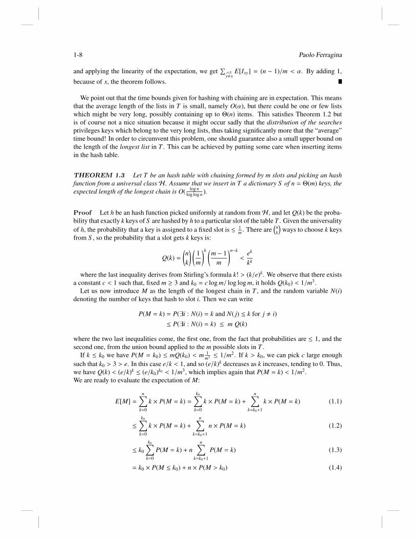
By combining together all these inequalities we can conclude that E[M] ≤ k0 + n(1/n) = k0 + 1 =

O(log m/ log log m), which is the thesis since we assumed m = Θ(n).

Two observations are in order at this point. The condition on m = Θ(n) can be easily guaranteedby applying the doubling method to the table T , as we showed in Theorem 1.2. The bound on themaximum chain length is on average, but it can be turned into worst case via a simple argument.We start by picking a random hash function h ∈ H , hash every key of S into T , and see whether thecondition on the length of the longest chain is at most twice the expected length log m/ log log m.If so, we use T for the subsequent search operations, otherwise we pick a new function h and re-insert all items in T . A constant number of trials suffice to satisfy that bound2, thus taking O(n)construction time in expectation.

FIGURE 1.4: Example of d-left hashing with four subtables, four hash functions, and each tableentry consisting of a bucket of a 4 slots.

Surprisingly enough, this result can be further improved by using two or more, say d, hash func-tions and d sub-tables T1,T2, ...,Td of the same size m/d, for a total space occupancy equal to theclassic single hash table T . Each table Ti is indexed by a different hash function hi ranging in0, 1, . . . ,m/d − 1. The specialty of this scheme resides in the implementation of the procedureInsert(k): it tests the loading of the d slots Ti[hi(k)], and inserts k in the sparsest one. In the caseof a tie, about slots’ loading, the algorithm chooses the leftmost table, i.e. the one with minimumindex i. For this reason this algorithmic scheme is also known as d-left hashing. The implementa-tion of Search(k) follows consequently, we need to search all d lists Ti[hi(k)] because we do notknow which were their loading when k was inserted, if any. The time cost for Insert(k) is O(d)time, the time cost of Search(k) is given by the total length of the d searched lists. We can upperbound this length by d times the length of the longest list in T which, surprisingly, can be proved tobe O(log log n), when d = 2, and it is log log n

log d + O(1) for larger d > 2. This result has to be compared

against the bound O( log nlog log n ) obtained for the case of a single hash function in Theorem 1.3. So, by

just using one more hash function, we can get an exponential reduction in the search time: this sur-

2Just use the Markov bound to state that the longest list longer than twice the average may occur with probability ≤ 1/2.

1-10 Paolo Ferragina

prising result is also known in the literature as the power of two choices, exactly because choosingbetween two slots the sparsest one allows to reduce exponentially the longest list.

As a corollary we notice that this result can be used to design a better hash table which does notuse chaining-lists to manage collisions, thus saving the space of pointers and increasing locality ofreference (hence less cache/IO misses). The idea is to allocate small and fixed-size buckets per eachslot, as it is illustrated in Figure 1.4. We can use two hash functions and buckets of size c log log n,for some small c > 1. The important implication of this result is that even for just two hash functionsthere is a large reduction in the maximum list length, and thus search time.

1.3.1 Do universal hash functions exist?

The answer is positive and, surprisingly enough, universal hash functions can be easily constructedas we will show in this section for three classes of them. We assume, without loss of generality,that the table size m is a prime number and keys are integers represented as bit strings of log2 |U |bits.3 We let r =

log2 |U |log2 m and assume that this is an integer. We decompose each key k in r parts, of

log2 m bits each, so k = [k0, k1, ...kr−1]. Clearly each part ki is an integer smaller than m, because itis represented in log2 m bits. We do the same for a generic integer a = [a0, a1, ..., ar−1] ∈ [0, |U | − 1]used as the parameter that defines the universal class of hash functions H as follows: ha(k) =∑r−1

i=0 aiki mod m. The size ofH is |U |, because we have one function per value of a.

THEOREM 1.4 The class H that contains the following hash functions: ha(k) =∑r−1

i=0 aiki

mod m, where m is prime and a is a positive integer smaller than |U |, is universal.

Proof Suppose that x and y are two distinct keys which differ, hence, on at least one bit. Forsimplicity of exposition, we assume that a differing bit falls into the first part, so x0 , y0. Accordingto Definition 1.1, we need to count how many hash functions make these two keys collide; orequivalently, how many a do exist for which ha(x) = ha(y). Since x0 , y0, and we operate inarithmetic modulo a prime (i.e. m), the inverse (x0 − y0)−1 must exist and it is an integer in the range[1, |U | − 1], and so we can write:

ha(x) = ha(y)⇔r−1∑i=0

aixi ≡

r−1∑i=0

aiyi ( mod m )

⇔ a0(x0 − y0) ≡ −r−1∑i=1

ai(xi − yi) ( mod m )

⇔ a0 ≡

− r−1∑i=1

ai(xi − yi)

(x0 − y0)−1 ( mod m )

The last equation actually shows that, whatever is the choice for [a1, a2, ..., ar−1] (and they aremr−1), there exists only one choice for a0 (the one specified in the last line above) which causes xand y to collide. As a consequence, there are mr−1 = |U |/m = |H|/m choices for [a1, a2, ..., ar−1]that cause x and y to collide. So the Definition 1.1 of Universal Hash class is satisfied.

3This is possible by pre-padding the key with 0, thus preserving its integer value.


It is possible to turn the previous definition holding for any table size m, thus not only for primevalues. The key idea is to make a double modular computation by means of a large prime p > |U |,and a generic integer m |U | equal to the size of the hash table we wish to set up. We canthen define an hash function parameterized in two values a ≥ 1 and b ≥ 0: ha,b(k) = ((ak +

b) mod p) mod m, and then define the familyHp,m =⋃

a>0,b≥0ha,b. It can be shown thatHp,m is auniversal class of hash functions.

The above two definitions require r multiplications and r modulo operations. There are indeedother universal hashing which are faster to be computed because they rely only on operations in-volving power-of-two integers. As an example take |U | = 2h, m = 2l < |U | and a be an odd integersmaller than |U |. Define the class Hh,l that contains the following hash functions: ha(k) = (akmod 2h) div 2h−l. This class contains 2h−1 distinct functions because a is odd and smaller than|U | = 2h. The following theorem presents the most important property of this class:

THEOREM 1.5 The classHh,l = ha(k) = (ak mod 2h) div 2h−l, with |U | = 2h and m = 2l <|U | and a odd integer smaller than 2h, is 2-universal because for any two distinct keys x and y, it is

P(ha(x) = ha(y)) ≤1

2l−1 =2m

.

Proof Without loss of generality let x > y and define A as the set of possible values for a (i.e. aodd integer smaller than 2h = |U |). If there is a collision ha(x) = ha(y), then we have:

ax mod 2h div 2h−l − ay mod 2h div 2h−l = 0|ax mod 2h div 2h−l − ay mod 2h div 2h−l| < 1

|ax mod 2h − ay mod 2h| < 2h−l

|a(x − y) mod 2h| < 2h−l

Set z = x − y > 0 (given that keys are distinct and x > y) and z < |U | = 2h, it is z . 0( mod 2h)and az . 0( mod 2h) because a is odd, so we can write:

az mod 2h ∈ 1, ..., 2h−l − 1 ∪ 2h − 2h−l + 1, ..., 2h − 1 (1.5)

In order to estimate the number of a ∈ A that satisfy this condition, we write z as z′2s with z′ oddand 0 ≤ s < h. The odd numbers a = 1, 3, 7, ..., 2h − 1 create a mapping a 7→ az′ mod 2h that is apermutation of A because z′ is odd. So, if we have the set a2s | a ∈ A, a possible permutation is sodefined: a2s 7→ az′2s mod 2h = az mod 2h. Thus, the number of a ∈ A that satisfy Eqn. 1.5 is thesame as the number of a ∈ A that satisfy:

a2s mod 2h ∈ 1, ..., 2h−l − 1 ∪ 2h − 2h−l + 1, ..., 2h − 1

Now, a2s mod 2h is the number represented by the h − s least significant bits of a, followed bys zeros. For example:

• If we take a = 7 , s = 1 and h = 3:7 ∗ 21 mod 23 is in binary 1112 ∗ 102 mod 10002 that is equal to 11102 mod 10002 =

1102. The result is represented by the h − s = 3 − 1 = 2 least significant bits of a,followed by s = 1 zeros.

• If we take a = 7 , s = 2 and h = 3:7∗22 mod 23 is in binary 1112∗1002 mod 10002 that is equal to 111002 mod 10002 =

1002. The result is represented by the h−s = 3−2 = 1 least significant bits of a, followedby s = 2 zeros.


• If we take a = 5 , s = 2 and h = 3:5∗22 mod 23 is in binary 1012∗1002 mod 10002 that is equal to 101002 mod 10002 =

1002. The result is represented by the h−s = 3−2 = 1 least significant bits of a, followedby s = 2 zeros.

So if s ≥ h − l there are no values of a that satisfy Eqn. 1.5, while for smaller s, the number ofa ∈ A satisfying that equation is at most 2h−l. Consequently the probability of randomly choosingsuch a is at most 2h−l/2h−1 = 1/2l−1. Finally, the universality of Hh,l follows immediately because

12l−1 <

1m .

1.4 Perfect hashing, minimal, ordered!

The most known algorithmic scheme in the context of hashing is probably that of hashing withchaining, which sets m = Θ(n) in order to guarantee an average constant-time search; but thatoptimal time-bound is on average, as most students forget. This forgetfulness is not erroneous inabsolute terms, because do indeed exist variants of hash tables that offer a constant-time worst-casebound, thus making hashing a competitive alternative to tree-based data structures and the de factochoice in practice. A crucial concept in this respect is perfect hashing, namely, a hash functionwhich avoids collisions among the keys to be hashed (i.e. the keys of the dictionary to be indexed).Formally speaking,

DEFINITION 1.3 A hash function h : U → 0, 1, . . . ,m − 1 is said to be perfect with respectto a dictionary S of keys if, and only if, for any pair of distinct keys k′, k′′ ∈ S , it is h(k′) , h(k′′).

An obvious counting argument shows that it must be m ≥ |S | = n in order to make perfect-hashingpossible. In the case that m = n, i.e. the minimum possible value, the perfect hash function is namedminimal (shortly MPHF). A hash table T using an MPHF h guarantees O(1) worst-case search time aswell as no waste of storage space, because it has the size of the dictionary S (i.e. m = n) and keyscan be directly stored in the table slots. Perfect hashing is thus a sort of “perfect” variant of direct-address tables (see Section 1.1), in the sense that it achieves constant search time (like those tables),but optimal linear space (unlike those tables).

A (minimal) perfect hash function is said to be order preserving (shortly OP(MP)HF) iff, ∀ki <k j ∈ S , it is h(ki) < h(k j). Clearly, if h is also minimal, and thus m = n; then h(k) returns the rankof the key in the ordered dictionary S . It goes without saying that, the property OP(MP)HF strictlydepends onto the dictionary S upon which h has been built: by changing S we could destroy thisproperty, so it is difficult, even if not impossible, to maintain this property under a dynamic scenario.In the rest of this section we will confine ourselves to the case of static dictionaries, and thus a fixeddictionary S .

The design of h is based upon three auxiliary functions h1, h2 and g, which are defined as follows:

• h1 and h2 are two universal hash functions from strings to 0, 1, . . . ,m′ − 1 picked ran-domly from a universal class (see Section 1.3). They are not necessarily perfect, andso they might induce collisions among S ’s keys. The choice of m′ impacts onto theefficiency of the construction, typically it is taken m′ = cn, where c > 1, so spanning arange which is larger than the number of keys.

• g is a function that maps integers in the range 0, . . . ,m′ − 1 to integers in the range0, . . . , n − 1. This mapping cannot be perfect, given that m′ ≥ n, and so some output


(a) Term t h1(t) h2(t) h(t) (b) x g(x)body 1 6 0 0 0cat 7 2 1 1 5dog 5 7 2 2 0flower 4 6 3 3 7house 1 10 4 4 8mouse 0 1 5 5 1sun 8 11 6 6 4tree 11 9 7 7 1zoo 5 3 8 8 0

9 110 811 6

TABLE 1.1 An example of an OPMPHF for a dictionary S of n = 9 strings which are in alphabetic

order. Column h(t) reports the lexicographic rank of each key; h is minimal because its values are in

0, . . . , n − 1 and is built upon three functions: (a) two random hash functions h1(t) and h2(t), for

t ∈ S ; (b) a properly derived function g(x), for x ∈ 0, 1, . . . ,m′. Here m′ = 11 > 9 = n.

values could be repeated. The function g is designed in a way that it properly combinesthe values of h1 and h2 in order to derive the OP(MP)HF h:

h(t) = ( g(h1(t)) + g(h2(t)) ) mod n

The construction of g is obtained via an elegant randomized algorithm which deployspaths in acyclic random graphs (see below).

Examples for these three functions are given in the corresponding columns of Table 1.1. Althoughthe values of h1 and h2 are randomly generated, the values of g are derived by a proper algorithmwhose goal is to guarantee that the formula for h(t) maps a string t ∈ S to its lexicographic rank inS . It is clear that the evaluation of h(t) takes constant time: we need to perform accesses to arrays h1and h2 and g, plus two sums and one modular operation. The total required space is O(m′+n) = O(n)whenever m′ = cn. It remains to discuss the choice of c, which impacts onto the efficiency of therandomized construction of g and onto the overall space occupancy. It is suggested to take c > 2,which leads to obtain a successful construction in

√ mm−2n trials. This means about two trials by

setting c = 3 (see [5]).

THEOREM 1.6 An OPMPHF for a dictionary S of n keys can be constructed in O(n) averagetime. The hash function can be evaluated in O(1) time and uses O(n) space (i.e. O(n log n) bits);both time and space bounds are worst case and optimal.

Before digging into the technical details of this solution, let us make an important observationwhich highlights the power of OPMPHF. It is clear that we could assign the rank to each string bydeploying a trie data structure (see Theorem ??), but this would incur two main limitations: (i) rankassignment would need a trie search operation which would incur Θ(s) I/Os, rather than O(1); (ii)space occupancy would be linear in the total dictionary length, rather than in the total dictionarycardinality. The reason is that, the OPMPHF’s machinery does not need the string storage thusallowing to pay space proportional to the number of strings rather than their length; but on the otherhand, OPMPHF does not allow to compute the rank of strings not in the dictionary, an operationwhich is instead supported by tries via the so called lexicographic search (see Chapter ??).


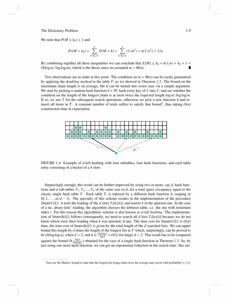
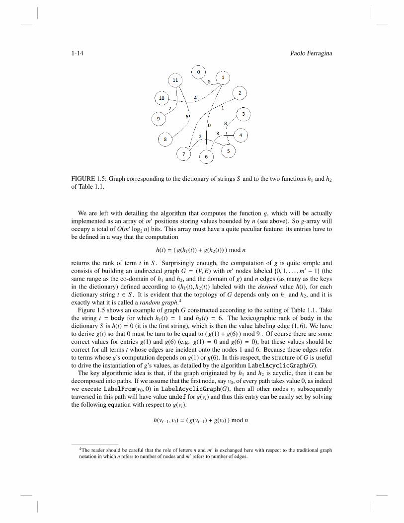
FIGURE 1.5: Graph corresponding to the dictionary of strings S and to the two functions h1 and h2of Table 1.1.

We are left with detailing the algorithm that computes the function g, which will be actuallyimplemented as an array of m′ positions storing values bounded by n (see above). So g-array willoccupy a total of O(m′ log2 n) bits. This array must have a quite peculiar feature: its entries have tobe defined in a way that the computation

h(t) = ( g(h1(t)) + g(h2(t)) ) mod n

returns the rank of term t in S . Surprisingly enough, the computation of g is quite simple andconsists of building an undirected graph G = (V, E) with m′ nodes labeled 0, 1, . . . ,m′ − 1 (thesame range as the co-domain of h1 and h2, and the domain of g) and n edges (as many as the keysin the dictionary) defined according to (h1(t), h2(t)) labeled with the desired value h(t), for eachdictionary string t ∈ S . It is evident that the topology of G depends only on h1 and h2, and it isexactly what it is called a random graph.4

Figure 1.5 shows an example of graph G constructed according to the setting of Table 1.1. Takethe string t = body for which h1(t) = 1 and h2(t) = 6. The lexicographic rank of body in thedictionary S is h(t) = 0 (it is the first string), which is then the value labeling edge (1, 6). We haveto derive g(t) so that 0 must be turn to be equal to ( g(1) + g(6) ) mod 9 . Of course there are somecorrect values for entries g(1) and g(6) (e.g. g(1) = 0 and g(6) = 0), but these values should becorrect for all terms t whose edges are incident onto the nodes 1 and 6. Because these edges referto terms whose g’s computation depends on g(1) or g(6). In this respect, the structure of G is usefulto drive the instantiation of g’s values, as detailed by the algorithm LabelAcyclicGraph(G).

The key algorithmic idea is that, if the graph originated by h1 and h2 is acyclic, then it can bedecomposed into paths. If we assume that the first node, say v0, of every path takes value 0, as indeedwe execute LabelFrom(v0, 0) in LabelAcyclicGraph(G), then all other nodes vi subsequentlytraversed in this path will have value undef for g(vi) and thus this entry can be easily set by solvingthe following equation with respect to g(vi):

h(vi−1, vi) = ( g(vi−1) + g(vi) ) mod n

4The reader should be careful that the role of letters n and m′ is exchanged here with respect to the traditional graphnotation in which n refers to number of nodes and m′ refers to number of edges.


Algorithm 1.1 Procedure LabelAcyclicGraph(G)1: for v ∈ V do2: g[v] = undef

3: end for4: for v ∈ V do5: if g[v] = undef then6: LabelFrom(v, 0)7: end if8: end for

which actually means to compute:

g(vi) = ( h(vi−1, vi) − g(vi−1) ) mod n

Algorithm 1.2 Procedure LabelFrom(v, c)1: if g[v] , undef then2: if g[v] , c then3: return - the graph is cyclic; STOP4: end if5: end if6: g[v] = c7: for u ∈ Adj[v] do8: LabelFrom(u, h(v, u) − g[v] mod n)9: end for

This is exactly what the algorithm LabelFrom(v, c) does. It is natural at this point to ask whetherthese algorithms always find a good assignment to function g or not. It is not difficult to convinceourselves that they return a solution only if the input graph G is acyclic, otherwise they stop. In thislatter case, we have to rebuild the graph G, and thus the hash functions h1 and h2 by drawing themfrom the universal class.

What is the likelihood of building an acyclic graph ? This question is quite relevant since thetechnique is useful only if this probability of success is large enough to need few rebuilding steps.According to Random Graph Theory [5], if m′ ≤ 2n this probability is almost equal to 0; otherwise,

if m′ > 2n then it is about√

m′−2nm′ , as we mentioned above. This means that the average number of

graphs we will need to build before finding an acyclic one is:√

m′m′−2n ; which is a constant number

if we take m′ = Θ(n). So, on average, the algorithm LabelAcyclicGraph(G) builds Θ(1) graphsof m′ + n = Θ(n) nodes and edges, and thus it takes Θ(n) time to execute those computations. Spaceusage is m′ = Θ(n).

In order to reduce the space requirements, we could resort multi-graphs (i.e. graphs with multipleedges between a pair of nodes) and thus use three hash functions, instead of two:

h (t) = (g (h1 (t)) + g (h2 (t)) + g (h3 (t))) mod n

We conclude this section by a running example that executes LabelAcyclicGraph(G) on thegraph in Figure 1.5.


1. Select node 0, set g(0) = 0 and start to visit its neighbors, which in this case is just thenode 1.

2. Set g(1) = (h(0, 1) − g(0))mod9 = (5 − 0)mod9 = 5.3. Take the unvisited neighbors of 1: 6 and 10, and visit them recursively.4. Select node 6, set g(6) = (h(1, 6) − g(1))mod9 = (0 − 5)mod9 = 4.5. Take the unvisited neighbors of 6: 4 and 10, the latter is already in the list of nodes to be

explored.6. Select node 10, set g(10) = (h(1, 10) − g(1))mod9 = (4 − 5)mod9 = 8.7. No unvisited neighbors of 10 do exist.8. Select node 4, set g(4) = (h(4, 6) − g(6))mod9 = (3 − 4)mod9 = 8.9. No unvisited neighbors of 4 do exist.

10. No node is left in the list of nodes to be explored.11. Select a new starting node, for example 2, set g(2) = 0, and select its unvisited neighbor

7.12. Set g(7) = (h(2, 7) − g(2))mod9 = (1 − 0)mod9 = 1, and select its unvisited neighbor 5.13. Set g(5) = (h(7, 5) − g(7))mod9 = (2 − 1)mod9 = 1, and select its unvisited neighbor 3.14. Set g(3) = (h(3, 5) − g(5))mod9 = (8 − 1)mod9 = 7.15. No node is left in the list of nodes to be explored.16. Select a new starting node, for example 8, set g(8) = 0, and select its unvisited neighbor

11.17. Set g(11) = (h(8, 11) − g(8))mod9 = (6 − 0)mod9 = 6, and select its unvisited neighbor

9.18. Set g(9) = (h(11, 9) − g(11))mod9 = (7 − 6)mod9 = 1.19. No node is left in the list of nodes to be explored.20. Since all other nodes are isolated, their g’s value is set to 0;

It goes without saying that, if S undergoes some insertions, we possibly have to rebuild h(t).Therefore, all of this works for a static dictionary S .

1.5 A simple perfect hash table

If ordering and minimality (i.e. h(t) < n) is not required, then the design of a (static) perfecthash function is simpler. The key idea is to use a two-level hashing scheme with universal hashingfunctions at each level. The first level is essentially hashing with chaining, where the n keys arehashed into m slots using a universal hash function h; but, unlike chaining, every entry T [ j] pointsto a secondary hash table T j which is addressed by another specific universal hash function h j.By choosing h j carefully, we can guarantee that there are no collisions at this secondary level. Thisway, the search for a key k will consist of two table accesses: one at T according to h, and one atsome Ti according to hi, given that i = h(k). For a total of O(1) time complexity in the worst case.

The question now is to guarantee that: (i) hash functions h j are perfect and thus elicit no collisionsamong the keys mapped by h into T [ j], and (ii) the total space required by table T and all sub-tablesT j is the optimal O(n). The following theorem is crucial for the following arguments.

THEOREM 1.7 If we store q keys in a hash table of size w = q2 using a universal hashfunction, then the expected number of collisions among those keys is less than 1/2. Consequently,the probability to have a collision is less than 1/2.


Proof In a set of q elements there are(

q2

)< q2/2 pairs of keys that may collide; if we choose the

function h from a universal class, we have that each pair collides with probability 1/w. If we setw = q2 the expected number of collisions is

(q2

)1w < q2/(2q2) = 1

2 . The probability to have at leastone collision can be upper bounded by using the Markov inequality (i.e. P(X ≥ tE[X]) ≤ 1/t), withX expressing the number of collisions and by setting t = 2.

We use this theorem in two ways: we will guarantee (i) above by setting the size m j of hash tableT j as n2

j (the square of the number of keys hashed to T [ j]); we will guarantee (ii) above by settingm = n for the size of table T . The former setting ensures that every hash function h j is perfect,by just two re-samples on average; the latter setting ensures that the total space required by thesub-tables is O(n) as the following theorem formally proves.

THEOREM 1.8 If we store n keys in a hash table of size m = n using a universal hash functionh, then the expected size of all sub-tables T j is less than 2n: in formula, E[

∑m−1j=0 n2

j ] < 2n wheren j is the number of keys hashing to slot j and the average is over the choices of h in the universalclass.

Proof Let us consider the following identity: a2 = a + 2(

a2

)which is true for any integer a > 0.

We have:

E[m−1∑j=0

n2j ] = E[

m−1∑j=0

(n j + 2(n j

2

))]

= E[m−1∑j=0

n j] + 2E[m−1∑j=0

(n j

2

)]

= n + 2E[m−1∑j=0

(n j

2

)]

The former term comes from the fact that∑m−1

j=0 n j equals the total number of items hashed in thesecondary level, and thus it is the total number n of dictionary keys. For the latter term we noticethat

(n j2

)accounts for the number of collisions among the n j keys mapped to T [ j], so that

∑m−1j=0

(n j2

)equals the number of collisions induced by the primary-level hash function h. By repeating theargument adopted in the proof of Theorem 1.7 and using m = n, the expected value of this sum is atmost

(n2

)1m =

n(n−1)2m = n−1

2 . Summing these two terms we derive that the total space required by thistwo-level hashing scheme is bounded by n + 2 n−1

2 = 2n − 1.

It is important to observe that every hash function h j is independent on the others, so that ifit generates some collisions among the n j keys mapped to T [ j], it can be re-generated withoutinfluencing the other mappings. Analogously if at the first level h generates more than zn collisions,for some large constant z, then we can re-generate h. These theorems ensure that the averagenumber of re-generations is a small constant per hash function. In the following subsections wedetail insertion and searching with perfect hashing.

Create a perfect hash table

In order to create a perfect hash table from a dictionary S of n keys we proceed as indicated in thepseudocode of Figure 1.3. Theorem 1.8 ensures that the probability to extract a good function from


the family Hp,m is at least 1/2, so we have to repeat the extraction process (at the first level) anaverage number of 2 times to guarantee a successful extraction, which actually means L < 2n. Atthe second level Theorem 1.7 and the setting m j = n2

j ensure that the probability to have a collisionin table T j because of the hash function h j is lower than 1/2. SO, again, we need on average twoextractions for h j to construct a perfect hash table T j.

Algorithm 1.3 Creating a Perfect Hash Table1: Choose a universal hash function h from the family Hp,m;2: for j = 0, 1, . . . ,m − 1 do3: n j = 0, S j = ∅;4: end for5: for k ∈ S do6: j = h(k);7: Add k to set S j;8: n j = n j + 1;9: end for

10: Compute L =∑m−1

j=0 (n j)2;11: if L ≥ 2n then12: Repeat the algorithm from Step 1;13: end if14: for j = 0, 1, . . . ,m − 1 do15: Construct table T j of size m j = (n j)2;16: Choose hash function h j from class Hp,m j ;17: for k ∈ S j do18: i = h j(k);19: if T j[i] , NULL then20: Destroy T j and repeat from step 15;21: end if22: T j[i] = k;23: end for24: end for

Searching keys with perfect hashing

Searching for a key k in a perfect hash table T takes just two memory accesses, as indicated in thepseudocode of Figure 1.4.

With reference to Figure 1.6, let us consider the successful search for the key 98 ∈ S . It ish(98) = ((2 × 98 + 42) mod 101) mod 11 = 3. Since T3 has size m3 = 4, we apply the second-levelhash function h3(98) = ((4 × 98 + 42) mod 101) mod 4 = 2. Given that T3(2) = 98, we have foundthe searched key.

Let us now consider the unsuccessful search for the key k = 8 < S . Since it is h(8) = ((2 ×8 + 42) mod 101) mod 11 = 3, we have to look again at the table T3 and compute h3(8) = ((4 ×8 + 42) mod 101) mod 4 = 2. Given that T3(2) = 19, we conclude that the key k = 8 is not in thedictionary.

1.6 Cuckoo hashing


FIGURE 1.6: Creating a perfect hash table over the dictionary S = 98, 19, 14, 50, 1, 72, 79, 3, 69,with h(k) = ((2k + 42) mod 101) mod 11. Notice that L = 1 + 1 + 4 + 4 + 4 + 1 = 15 < 2 × 9and, at the second level, we use the same hash function changing only the table size for the modulocomputation. There no collision occur.

When the dictionary is dynamic a different hashing scheme has to be devised, an efficient andelegant solution is the so called cuckoo hashing: it achieves constant time in updates, on average,and constant time in searches, in the worst case. The only drawback of this approach is that itmakes use of two hash functions that are O(log n)-independent (new results in the literature havesignificantly relaxed this requirement [1] but we stick on the original scheme for its simplicity). Inpills, cuckoo hashing combines the multiple-choice approach of d-left hashing with the ability tomove elements. In its simplest form, cuckoo hashing consists of two hash functions h1 and h2 andone table T of size m. Any key k is stored either at T [h1(k)] or at T [h2(k)], so that searching anddeleting operations are trivial: we need to look for k in both those entries, and eventually remove it.Inserting a key is a little bit more tricky in that it can trigger a cascade of key moves in the table.Suppose a new key k has to be inserted in the dictionary, according to the Cuckoo scheme it has tobe inserted either at position h1(k) or at position h2(k). If one of these locations in T is empty (ifboth are, h1(k) is chosen), the key is stored at that position and the insertion process is completed.Otherwise, both entries are occupied by other keys, so that we have to create room for k by evictingone of the two keys stored in those two table entries. Typically, the key y stored in T [h1(k)] isevicted and replaced with k. Then, y plays the role of k and the insertion process is repeated.

There is a warning to take into account at this point. The key y was stored in T [h1(k)], so thatT [hi(y)] = T [h1(k)] for either i = 1 or i = 2. This means that if both positions T [h1(y)] and T [h2(y)]are occupied, the key to be evicted cannot be chosen from the entry that was storing T [h1(k)] becauseit is k, so this would induce a trivial infinite cycle of evictions over this entry between keys k and y.The algorithm therefore is careful to always avoid to evict the previously inserted key. Neverthelesscycles may arise (e.g. consider the trivial case in which h1(k), h2(k) = h1(y), h2(y)) and they canbe of arbitrary length, so that the algorithm must be careful in defining an efficient escape conditionwhich detects those situations, in which case it re-sample the two hash functions and re-hash alldictionary keys. The key property, proved in Theorem 1.9, will be to show that cycles occurs with


Algorithm 1.4 Procedure Search(k) in a Perfect Hash Table T1: Let h and h j be the universal hash functions defining T ;2: Compute j = h(k);3: if T j is empty then4: Return false; // k < S5: end if6: Compute i = h j(k);7: if T j[i] = NULL then8: Return false; // k < S9: end if

10: if T j[i] , k then11: Return false; // k < S12: end if13: Return true; // k ∈ S

bounded probability, so that the O(n) cost of re-hashing can be amortized, by charging O(1) timeper insertion (Corollary 1.4).

FIGURE 1.7: Graphical representation of cuckoo hashing.

In order to analyze this situation it is useful to introduce the so called cuckoo graph (see Figure1.7), whose nodes are entries of table T and edges represent dictionary keys by connecting the twotable entries where these keys can be stored. Edges are directed to keep into account where a key isstored (source), and where a key could be alternatively stored (destination). This way the cascadeof evictions triggered by key k traverses the nodes (table entries) laying on a directed path that startsfrom either node (entry) h1(k) or node h2(k). Let us call this path the bucket of k. The bucket remindsthe list associated to entry T [h(k)] in hashing with chaining (Section 1.2), but it might have a morecomplicated structure because the cuckoo graph can have cycles, and thus this path can form loopsas it occurs for the cycle formed by keys W and H.

For a more detailed example of insertion process, let us consider again the cuckoo graph depictedin Figure 1.7. Suppose to insert key D into our table, and assume that h1(D) = 4 and h2(D) = 1, sothat D evicts either A or B (Figure 1.8). We put D in table entry 1, thereby evicting A which tries tobe stored in entry 4 (according to the directed edge). In turn, A evicts B, stored in 4, which is movedto the last location of the table as its possible destination. Since such a location is free, B goes thereand the insertion process is successful and completed. Let us now consider the insertion of key F,and assume two cases: h1(F) = 2 and h2(F) = 5 (Figure 1.9.a), or h1(F) = 4 and h2(F) = 5 (Figure1.9.b). In the former case the insertion is successful: F causes C to be evicted, which in turn finds thethird location empty. It is interesting to observe that, even if we check first h2(F), then the insertion


is still successful: F causes H to be evicted, which causes W to be evicted, which in turn causes againF to be evicted. We found a cycle which nevertheless does not induces an infinite loop, in fact in thiscase the eviction of F leads to check its second possible location, namely h1(F) = 2, which evicts Cthat is then stored in the third location (currently empty). Consequently the existence of a cycle doesnot imply an unsuccessful search; said this, in the following, we will compute the probability of theexistence of a cycle as an upper bound to the probability of an unsuccessful search. Conversely,the case of an unsuccessful insertion occurs in Figure 1.9.b where there are two cycles F-H andA-B which gets glued together by the insertion of the key F. In this case the keys flow from onecycle to the other without stopping. As a consequence, the insertion algorithm must be designed inorder to check whether the traversal of the cuckoo graph ended up in an infinite loop: this is doneapproximately by bounding the number of eviction steps.

FIGURE 1.8: Inserting the key D: (left) the two entry options, (right) the final configuration.

FIGURE 1.9: Inserting the key F: (left) successful insertion, (right) unsuccessful insertion.

1.6.1 An analysis

Querying and deleting a key k takes constant time, only two table entries have to be checked. Thecase of insertion is more complicated because it has necessarily to take into account the formationof paths in the (random) cuckoo graph. In the following we consider an undirected cuckoo graph,namely one in which edges are not oriented, and observe that a key y is in the bucket of another keyx only if there is a path between one of the two positions (nodes) of x and one of the two positions(nodes) of y in the cuckoo graph. This relaxation allows to easy the bounding of the probability ofthe existence of these paths (recall that m is the table size and n is the dictionary size):


THEOREM 1.9 For any entries i and j and any constant c > 1, if m ≥ 2cn, then the probabilitythat in the undirected cuckoo graph there exists a shortest path from i to j of length L ≥ 1 is at mostc−L/m.

Proof We proceed by induction on the path length L. The base case L = 1 corresponds to theexistence of the undirected edge (i, j); now, every key can generate that edge with probability nomore than ≤ 2/m2, because edge is undirected and h1(k) and h2(k) are uniformly random choicesamong the m table entries. Summing over all n dictionary keys, and recalling that m ≥ 2cn, we getthe bound

∑k∈S 2/m2 = 2n/m2 ≤ c−1/m.

For the inductive step we must bound the probability that there exists a path of length L > 1, butno path of length less than L connects i to j (or vice versa). This occurs only if, for some table entryh, the following two conditions hold:

• there is a shortest path of length L − 1 from i to z (that clearly does not go through j);• there is an edge from z to j.

By the inductive hypothesis, the probability that the first condition is true is bounded by c−(L−1)/m =

c−L+1/m. The probability of the second condition has been already computed and it is at mostc−1/m = 1/cm. So the probability that there exists such a path (passing through z) is (1/cm) ∗(c−L+1/m) = c−L/m2. Summing over all m possibilities for the table entry z, we get that the proba-bility of a path of length L between i and j is at most c−L/m.

In other words, this Theorem states that if the number m of nodes in the cuckoo graph is suffi-ciently large compared to the number n of edges (i.e. m ≥ 2cn), there is a low probability that anytwo nodes i and j are connected by a path, thus fall in the same bucket, and hence participate in acascade of evictions. Very significant is the case of a constant-length path L = O(1), for which theprobability of occurrence is O(1/m). This means that, even for this restricted case, the probabilityof a large bucket is small and thus the probability of a not-constant number of evictions is small. Wecan related this probability to the collision probability in hashing with chaining. We have thereforeproved the following:

THEOREM 1.10 For any two distinct keys x and y, the probability that x hashes to the samebucket of y is O(1/m).

Proof If x and y are in the same bucket, then there is a path of some length L between one nodein h1(x), h2(x) and one node in h1(y), h2(y). By Theorem 1.9, this occurs with probability at most4∑∞

L=1 c−L/m = 4c−1/m = O(1/m), as desired.

What about rehashing? How often do we have to rebuild table T? Let us consider a sequence ofoperations involving εn insertions, where ε is a small constant, e.g. ε = 0.1, and assume that thetable size is sufficiently large to satisfy the conditions imposed in the previous theorems, namelym ≥ 2cn + 2c(εn) = 2cn(1 + ε). Let S ′ be the final dictionary in which all εn insertions have beenperformed. Clearly, there is a re-hashing of T only if some key insertion induced an infinite loop inthe cuckoo graph. In order to bound this probability we consider the final graph in which all keys S ′

have been inserted, and thus all cycles induced by their insertions are present. This graph consistsof m nodes and n(1 + ε) keys. Since we assumed m ≥ 2cn(1 + ε), according to the Theorem 1.9, anygiven position (node) is involved in a cycle (of any length) if it is involved in a path (of any length)that starts and end at that position: the probability is at most

∑∞L=1 c−L/m. Thus, the probability

that there is a cycle of any length involving any table entry can be bounded by summing over all m


table entries: namely, m∑∞

L=1 c−L/m = 1c−1 . As we observed previously, this is an upper bound to

the probability of an unsuccessful insertion given that the presence of a cycle does not necessarilyimply an infinite loop for an insertion.

COROLLARY 1.3 By setting c = 3, and taking a cuckoo table of size m ≥ 6n(1 + ε), theprobability for the existence of a cycle in the cuckoo graph of the final dictionary S ′ is at most 1/2.

Therefore a constant number of re-hashes are enough to ensure the insertion of εn keys in adictionary of size n. Given that the time for one rehashing is O(n) (we just need to compute twohashes per key), the expected time for all rehashing is O(n), which is O(1/ε) per insertion.

COROLLARY 1.4 By setting c > 2, and taking a cuckoo table of size m ≥ 2cn(1 + ε), the costfor inserting εn keys in a dictionary of size n by cuckoo hashing is constant expected amortized.Namely, expected with respect to the random selection of the two universal hash functions drivingthe cuckoo hashing, and amortised over the Θ(n) insertions.

In order to make the algorithm works for every n and ε, we can adopt the same idea sketched forhashing with chaining and called global rebuilding technique. Whenever the size of the dictionarybecomes too small compared to the size of the hash table, a new, smaller hash table is created;conversely, if the hash table fills up to its capacity, a new, larger hash table is created. To make thiswork efficiently, the size of the hash table is increased or decreased by a constant factor (larger than1), e.g. doubled or halved.

The cost of rehashing can be further reduced by using a very small amount (i.e. constant) ofextra-space, called a stash. Once a failure situation is detected during the insertion of a key k (i.e. kincurs in a loop), then this key is stored in the stash (without rehashing). This reduces the rehashingprobability to Θ(1/ns+1), where s is the size of the stash. The choice of parameter s is related tosome structural properties of the cuckoo graph and of the universal hash functions, which are tooinvolved to be commented here (for details see [1] and refs therein).

1.7 Bloom filters

There are situations in which the universe of keys is very large and thus every key is long enoughto take a lot of space to be stored. Sometimes it could even be the case that the storage of tablepointers, taking (n+m) log n bits, is much smaller than the storage of the keys, taking n log2 |U | bits.An example is given by the dictionary of URLs managed by crawlers in search engines; maintainingthis dictionary in internal memory is crucial to ensure the fast operations over those URLs requiredby crawlers. However URLs are thousands of characters long, so that the size of the indexable dic-tionary in internal memory could be pretty much limited if whole URLs should have to be stored.And, in fact, crawlers do not use neither cuckoo hashing nor hashing with chaining but, rather, em-ploy a simple and randomised, yet efficient, data structure named Bloom filter. The crucial propertyof Bloom filters is that keys are not explicitly stored, only a small fingerprint of them is, and this in-duces the data structure to make a one-side error in its answers to membership queries whenever thequeried key is not in the currently indexed dictionary. The elegant solution proposed by Bloom fil-ters is that those errors can be controlled, and indeed their probability decreases exponentially withthe size of the fingerprints of the dictionary keys. Practically speaking tens of bits (hence, few bytes)


per fingerprint are enough to guarantee tiny error probabilities5 and succinct space occupancy, thusmaking this solution much appealing in a big-data context. It is useful at this point recall the Bloomfilter principle: “Wherever a list or set is used, and space is a consideration, a Bloom filter shouldbe considered. When using a Bloom filter, consider the potential effects of false positives”.

Let S = x1, x2, ..., xn be a set of n keys and B a bit vector of length m. Initially, all bits in Bare set to 0. Suppose we have r universal hash functions hi : U −→ 0, ...,m − 1, for i = 1, ..., r.As anticipated above, every key k is not represented explicitly in B but, rather, it is fingerprinted bysetting r bits of B to 1 as follows: B[hi(k)] = 1, ∀ 1 ≤ i ≤ r. Therefore, inserting a key in a Bloomfilter requires O(r) time, and sets at most r bits (possibly some hashes may collide, this is calledstandard Bloom Filter). For searching, we claim that a key y is in S if B[hi(y)] = 1, ∀ 1 ≤ i ≤ r.Searching costs O(r), as well as inserting. In the example of Figure 1.10, we can assert that y < S ,since three bits are set to 1 but the last checked bit B[h4(y)] is zero.

FIGURE 1.10: Searching key y in a Bloom filter.

Clearly, if y ∈ S the Bloom filter correctly detects this; but it might be the case that y < S andnonetheless all r bits checked are 1 because of the setting due to other hashes and keys. This is calledfalse positive error, because it induces the Bloom filter to return a positive but erroneous answer toa membership query. It is therefore natural to ask for the probability of a false-positive error, whichcan be proved to be bounded above by a surprisingly simple formula.

The probability that the insertion of a key k ∈ S has left null a bit-entry B[ j] equals the probability

that the r independent hash functions hi(k) returned an entry different of j, which is(

m−1m

)r≈ e−

rm .

After the insertion of all n dictionary keys, the probability that B[ j] is still null can be then bounded

by p0 ≈

(e−

rm

)n= e−

rnm by assuming independencies among those hash functions.6 Hence the

probability of a false-positive error (or, equivalently, the false positive rate) is the probability thatall r bits checked for a key not in the current dictionary are set to 1, that is:

perr = (1 − p0)r ≈(1 − e−

rnm

)r

Not surprisingly the error probability depends on the three parameters that define the Bloomfilter’s structure: the number r of hash functions, the number n of dictionary keys, and the numberm of bits in the binary array B. It’s interesting to notice that the fraction f = m/n can be read as theaverage number of bits per dictionary key allocated in B, hence the fingerprint size f . The larger is

5One could object that, errors anyway might occur. But programmers counteract by admitting that these errors can bemade smallers than hardware/network errors in data centers or PCs. So they can be neglected!6A more precise analysis is possible, but much involved and without changing the final result, so that we prefer to stickon this simpler approach.


f the smaller is the error probability perr, but the larger is the space allocated for B. We can optimizeperr according to m and n, by computing the first-order derivative and equalling it to zero: this getsr = m

n ln 2. It is interesting to observe that for this value of r the probability a bit in B gets null valueis p0 = 1/2; which actually means that the array is half filled by 1s and half by 0s. And indeed thisresult could not be different: a larger r induces more 1s in B and thus a larger probability of positiveerrors, a lower r induces more 0s in B and thus a larger probability of correct answers: the correctchoice of r falls in the middle! For this value of r = m

n ln 2, we have perr = (0.6185)m/n whichdecreases exponentially with the fingerprint size f = m/n. Figure 1.11 reports the false positive rateas a function of the number r of hashes for a Bloom-filter designed to use m = 32n bits of space,hence a fingerprint of f = 32 bits per key. By using 22 hash functions we can minimize the falsepositive rate to less than 1.E − 6. However, we also note that adding one more hash function doesnot significantly decreases the error rate when r ≥ 10.

FIGURE 1.11: Plotting perr as a function of the number of hashes.

It is natural now to derive the size m of the B-array whenever r is fixed to its optimal value mn ln 2,

and n is the number of current keys in the dictionary. We obtain different values of perr depending onthe choice of m. For example, if m = n then perr = 0.6185, if m = 2n then perr = 0.38, and if m = 5nwe have perr = 0.09. In practice m = cn is a good choice, and for c > 10 the error rate is interestinglysmall and useful for practical applications. Figure 1.12 compares the performance of hashing (withchaining) to that of Bloom filters, assuming that the number r of used hash functions is the onewhich minimizes the false-positive error rate. In hashing with chaining, we need Θ(n(log n + log u))bits to store the pointers in the chaining lists, and Θ(m log n is the space occupancy of the table, inbits. Conversely the Bloom filter does not need to store keys and thus it incurs only in the cost ofstoring the bit array m = f n, where f is pretty small in practice as we observed above.

As a final remark we point out that they do exist other versions of the Bloom Filter, the mostnotable ones are the so called classic Bloom Filter, in which it is assumed that the r bits set to oneare all distinct, and the partitioned Bloom Filter, in which the distinctness of the set bits is achievedby dividing the array B in r parts and setting one bit each. In [3] it is provided a detailed probabilisticanalysis of classic and standard Bloom Filters: the overall result is that the average number of setbits is the same as well as very similar is the false-match probability, the difference concerns withthe variance of set bits which is slightly larger in the case of the classic data structure. However,


this does not impact significantly in the overall error performance in practice.

FIGURE 1.12: Hashing vs Bloom filter

1.7.1 A lower bound on space

The question is how small can be the bit array B in order to guarantee an given error rate ε for adictionary of n keys drawn from a universe U of size u. This lower bound will allow us to provethat space-wise Bloom filters are within a factor of log2 e ≈ 1.44 of the asymptotic lower bound.

The proof proceeds as follows. Let us represent any data structure solving the membership queryon a dictionary X ⊆ U with those time/error bounds with a m-bit string F(X). This data structuremust work for every possible subset of n elements of U, they are

(un

). We say that an m-bit string s

accepts a key x if s = F(X) for some X containing x, otherwise we say that s rejects x. Now, let usconsider a specific dictionary X of n elements. Any string s that is used to represent X must accepteach one of the n elements of X, since no false negatives are admitted, but it may also accept at mostε(u − n) other elements of the universe, thus guaranteeing a false positive rate smaller than ε. Eachstring s therefore accepts at most n + ε(u− n) elements, and can thus be used to represent any of the(

n+ε(u−n)n

)subsets of size n of these elements, but it cannot be used to represent any other set. Since

we are interested into data structures of m bits, they are 2m, and we are asking ourselves whetherthey can represent all the

(un

)possible dictionaries of U of n keys. Hence, we must have:

2m ×(

n+ε(u−n)n

)≥

(un

)or, equivalently:

m ≥ log2

(un

)/(

n+ε(u−n)n

)≥ log2

(un

)/(εun

)≥ log2 ε

−n = n log2(1/ε)

where we used the inequalities ( ab )b ≤

(ab

)≤ ( ae

b )b and the fact that in pratice it is u n. If weconsider a Bloom filter with the same configuration— namely, error rate ε and space occupancy mbits—, then we have ε = (1/2)r ≥ (1/2)m ln 2/n by setting r to the optimal number of hash functions.After some algebraic manipulations, we find that:

m ≥ n log2(1/ε)ln 2 ≈ 1.44 n log2(1/ε)

This means that Bloom filters are asymptotically optimal in space, the constant factor is 1.44 morethan the minimum possible.


1.7.2 Compressed Bloom filters

In many Web applications, the Bloom filter is not just an object that resides in memory, but it isa data structure that must be transferred between proxies. In this context it is worth to investigatewhether Bloom filters can be compressed to save bandwidth and transfer time [4]. Suppose that weoptimize the false positive rate of the Bloom filter under the constraint that the number of bits to besent after compression is z ≤ m. As compression tool we can use Arithmetic coding (see Chapter??), which well approximates the entropy of the string to be compressed: here simply expressed as−(p(0) log2 p(0)+p(1) log2 p(1)) where p(b) is the frequency of bit b in the input string. Surprisinglyenough it turns out that using a larger, but sparser, Bloom filter can yield the same false positive ratewith a smaller number of transmitted bits. Said in other words, one can transmit the same number ofbits but reduce the false positive rate. An example is given in Table 1.2, where the goal is to obtainsmall false positive rates by using less than 16 transmitted bits per element. Without compression,the optimal number of hash functions is 11, and the false positive rate is 0.000459. By making asparse Bloom filter using 48 bits per element but only 3 hash functions, one can compress the resultdown to less than 16 bits per item (with high probability) and decrease the false positive rate byroughly a factor of 2.

Array bits per element m/n 16 28 48Transmission bits per element z/n 16 15,846 15,829

Hash functions k 11 4 3False positive probability f 0,000459 0,000314 0,000222

TABLE 1.2 Using at most sixteen bits per element after compression, a bigger but sparser Bloom filter

can reduce the false positive rate.

Compressing a Bloom filter has benefits: (i) it uses a smaller number of hash functions, so that thelookups are more efficient; (ii) it may reduce the false positive rate for a desired compressed size, orreduce the transmited size for a fixed false positive rate. However the size m of the uncompressedBloom filter increases the memory usage at running time, and comes at the computational costof compressing/decompressing it. Nevertheless, some sophisticate approaches are possible whichallow to access directly the compressed data without incurring in their decompression. An examplewas given by the FM-index in Chapter ??, which could built over the bit-array B.

1.7.3 Spectral Bloom filters

A spectral bloom filter (SBF) is an extension of the original Bloom filter to multi-sets, thus allowingthe storage of multiplicities of elements, provided that they are below a given threshold (a spectrumindeed). SBF supports queries on the multiplicities of a key with a small error probability over itsestimate, using memory only slightly larger than that of the original Bloom filter. SBF supports alsoinsertions and deletions over the data set.

Let S be a multi-set consisting of n distinct keys from U and let fx be the multiplicity of theelement x ∈ S . In a SBF the bit vector B is replaced by an array of counters C[0,m − 1], where C[i]is the sum of fx-values for those elements x ∈ S mapping to position i. For every element x, we addthe value fx to the counters C[h1(x)],C[h2(x)], ...,C[hr(x)]. Due to possible conflicts among hashesfor different elements, the C[i]s provide approximated values, specifically upper bounds (given thatfx > 0.

The multi-set S can be dynamic. When inserting a new item s, its frequency fs increases by one,so that we increase by one the counters C[h1(s)],C[h2(s)], . . . ,C[hr(s)]; deletion consists symmet-


rically in decreasing those counters. In order to search for the frequency of element x, we simplyreturn the minimum value mx = mini C[hi(x)]. Of course, mx is a biased estimator for fx. In partic-ular, since all fx ≤ C[hi] for all i, the case in which the estimate is wrong (i.e. mx < fx) correspondsto the event “all counters C[hi(x)] have a collision”, which in turn corresponds to a “false positive”event in the classical Bloom filter. So, the probability of error in a SBF is the error rate probabilityfor a Bloom filter with the same set of parameters m, n, r.

1.7.4 A simple application

Bloom filters can be used to approximate the intersection of two sets, say A and B, stored in twomachines MA and MB. We wish to compute A ∩ B distributively, by exchanging a small number ofbits. Typical applications of the problem are data replication check and distributed search engines.The problem can be efficiently solved by using Bloom filters BF(A) and BF(B) stored in MA andMB, respectively. The algorithmic idea to compute A ∩ B is as follows:

1. MA sends BF(A) to MB, using ropt = (mAln2)/|A| hash functions and a bit-array mA =

Θ(|A|);2. MB checks the existence of elements B into A by deploying BF(A) and sends back

explicitly the set of found elements, say Q. Note that, in general, Q ⊇ A ∩ B because offalse positives;

3. MA computes Q ∩ A, and returns it.

Since Q contains |A ∩ B| keys plus the number of false positives (elements belonging only to A),we can conclude that |Q| = |A ∩ B| + |B|ε where ε = 0.6185mA/|A| is the error rate for that designof BF(A). Since we need log |U | bits to represent each key, the total number of exchanged bits isΘ(|A|) + (|A ∩ B| + |B|0.6185mA/|A|) log |U | which is much smaller than |A| log |U | the number of bitsto be exchanged by using a plain algorithm that sends the whole A’s set to MB.

References

[1] Martin Aumuller, Martin Dietzfelbinger, and Philipp Woelfel. Explicit and Efficient

Hash Families Suffice for Cuckoo Hashing with a Stash. In Proceedings of European

Symposium on Algorithms (ESA), Lecture Notes in Computer Science 7501, Springer,

108–120, 2012.

[2] Andrei Z. Broder and Michael Mitzenmacher. Survey: Network Applications of Bloom

Filters: A Survey. Internet Mathematics, 1(4): 485-509, 2003.

[3] Fabio Grandi. On the analysis of Bloom Filters. Information Processing Letters, 129:

35-39, 2018.

[4] Michael Mitzenmacher. Compressed bloom filters. IEEE/ACM Transactions on Networks,10(5): 604-612, 2002.

[5] Ian H. Witten, Alistair Moffat and Timothy C. Bell. Managing Gigabytes: Compressing

and Indexing Documents and Images, Second Edition. Morgan Kaufmann, 1999.