The Long-Term Impact of Steel Tariffson U.S. Manufacturing

Lydia Cox∗

Harvard University

November 7, 2021

Click here for latest version.

Abstract

In this paper, I study the long-term effects that temporary upstream tariffs have ondownstream industries. Even temporary tariffs can have cascading effects through pro-duction networks when placed on upstream products, but to date, little is known aboutthe long-term behavior of these spillovers. Using a new method for mapping down-stream industries to specific steel inputs, I estimate the effect of steel tariffs enactedby President Bush in 2002 and 2003 on downstream industry outcomes. I find thatupstream steel tariffs have highly persistent negative impacts on the competitiveness ofU.S. downstream industry exports. Persistence in the response of exports is driven by arestructuring of global trade flows that does not revert once the tariffs are lifted. I usea dynamic model of trade to show that the presence of relationship-specific sunk costsof exporting can generate persistence of the magnitude that I find in the data. Finally,I show that taking both the contemporaneous and persistent downstream impacts intoaccount substantially alters the welfare implications of upstream tariffs.

Keywords: Trade policy, tariff, global value chains, gains from trade, sunk cost,welfare.

JEL Codes: F10, F12, F13, F14

∗Harvard University, Department of Economics. lcox@g.harvard.edu. I am extremely grateful to myadvisors Pol Antras and Marc Melitz for numerous discussions regarding this work. I have also benefitedgreatly from conversations with Miguel Acosta, Elhanan Helpman, Ken Rogoff, Kathryn Russ, and RaphaelSchoenle. I would also like to thank participants in the Graduate Student Workshop in International Eco-nomics at Harvard and the Cowles Summer Conference in International Trade for insightful questions andfeedback.

1 Introduction

U.S. trade policy under the Trump administration sparked renewed attention to the fact

that globally integrated supply chains complicate the traditional cost-benefit analysis of

tariffs. Tariffs and other emergency safeguards are often justified as temporary measures

designed to relieve struggling domestic industries. When placed on upstream products,

however, this protection comes at a cost: Tariffs on upstream products raise input costs for

downstream manufacturers, making them more vulnerable to foreign competition. While

the tariffs themselves are temporary, little is known about the long-term behavior of these

spillover effects. This is the primary focus of my paper.

While the breadth and scale of the Trump administration’s protectionist efforts was

unprecedented in recent history, protectionist policy for certain U.S. industries is not a new

phenomenon.1 In this paper, I use a case study of the steel tariffs levied by George W. Bush

in 2002 and 2003 to provide new empirical evidence on the long-term effects that temporary

upstream tariffs have on downstream industries. Because steel is a broadly used input—Cox

and Russ (2020), for example, find that the number of jobs in industries that use steel as an

input outnumber the number of jobs that produce steel by about 80 to 1—tariffs on steel

are particularly prone to having broad downstream effects. This feature, along with the

fact that the Bush tariffs were a sizable but temporary shock to steel tariff rates, makes the

episode useful for studying both the contemporaneous and long-term downstream impacts

of temporary upstream tariffs. To generalize my empirical findings outside of this context

and understand the underlying mechanisms, I calibrate a dynamic model of trade, consistent

with my findings.

A key empirical challenge in estimating the causal impacts of upstream tariffs through

supply chains is linking protected upstream inputs to the downstream industries that use

them. Tariffs are placed on highly disaggregated products, rendering publicly available input-

output tables too coarse to provide the required mapping. A key innovation in this paper

is the creation of a highly detailed, steel-specific input-output table that links disaggregated

steel products to specific downstream industries. I create this new table using exclusion

requests for steel products that were submitted by firms in response to the Trump steel tariffs.

I take advantage of the fact that, by definition, exclusion requesting firms are downstream

users of very specific upstream products. With these data, I create a detailed mapping that

allows me to leverage the variation in tariff rates imposed by Bush in 2002 and 2003 to

causally estimate the impacts of higher tariff rates on downstream industry outcomes.

1Upstream products—like steel, aluminum, lumber, and sugar—that are central inputs to many U.S.manufacturing industries have enjoyed spurts of protectionist policy since this nation’s founding, accordingto Irwin (2017).

1

My primary empirical findings are threefold. First, I find that upstream steel tariffs

have highly persistent negative impacts on the competitiveness of U.S. downstream industry

exports. A 1 percentage point increase in an industry’s upstream steel tariff rate causes a

relative decline in the U.S. share of that industry’s world exports—or the industry’s global

market share—of 0.1 percentage points at its peak (0.2 percentage points for steel-intensive

industries). To put the magnitude of the impact into perspective, shifting an industry from

the 25th to the 75th percentile of the tariff burden distribution (an increase of 13.5 percentage

points) results in a decline in global market share of 1 percentage point relative to pre-tariff

levels (2 percentage points for steel-intensive industries). Declines in the competitiveness of

U.S. exports due to the tariffs are highly persistent—global market share remains depressed

relative to pre-tariff levels for at least 8 years after the tariffs are lifted. Likely a result of this

loss in market share, I also find that steel-intensive industries suffered persistent declines in

employment in response to relatively high steel tariff rates.

Second, I find that the persistence of the impact of steel tariffs on downstream exports

stems from a restructuring of global trade flows that does not revert once the tariffs are lifted.

Downstream industries that faced higher steel tariffs suffered persistent relative declines in

both export prices and quantities after the tariffs were lifted, consistent with an inward

shift of world demand for U.S. downstream products. I show that higher steel tariffs in

the U.S. led to relative increases in the downstream export shares of other top producing

countries. Germany, Japan, and France, in particular, experienced increases in their export

shares relative to pre-tariff levels that persisted after the tariffs were removed. This pattern

suggests that the U.S. steel tariffs induced a shift in sourcing patterns for foreign buyers in

downstream industries that did not revert when the tariffs were removed.

Third, I find that the impact of the steel tariffs on downstream domestic production

is more transitory than the impact on exports. I find that U.S. imports of downstream

products that faced a 1 percent higher steel tariff increased by 1 percent relative to pre-tariff

levels, suggesting that U.S. consumers substituted toward foreign sources when the tariffs

were in place. Imports revert to pre-tariff levels within two years of the tariffs being removed,

however, indicating that production for the domestic market rebounded much more quickly

than exports.

In the last part of the paper, I use a dynamic model of trade to show that the presence of

relationship-specific sunk costs of exporting can generate a persistent response of downstream

exports to an input tariff that is consistent with the patterns I find in the data. The

model features asymmetric countries, an upstream steel sector, heterogeneous Melitz-style

downstream steel users, and a relationship-specific sunk cost of trade that drives the key

results. Intuitively, because it is costly for countries to change sources of imports, if an

2

input tariff induces a change in sourcing patterns, those patterns will not immediately revert

when the tariffs are lifted. Using the model, I estimate the aggregate welfare implications

of a 2-year shock to steel tariffs in the home country that matches my empirical setting. I

find annual welfare losses equivalent to an average of 2.8 percent of exports that continue

to accrue for 8 years after the tariffs are removed. The model-implied estimates are in

line with reduced-form estimates that I calculate using a partial-equilibrium framework. A

counterfactual simulation in which I double the amount of time the tariffs are in place (from

2 to 4 years) leads to a doubling of aggregate welfare losses,2 suggesting that the longer input

tariffs are in place, the more distortionary they become.

My paper contributes to the growing empirical literature on the many channels through

which trade policy can affect the domestic economy. Among others, this literature includes

the work of Amiti et al. (2019), Cavallo et al. (2019), and Fajgelbaum et al. (2020), who

estimate the impacts of the Trump tariffs on prices and welfare. A subset of this literature

focuses, as I do, on the effect of tariffs through supply chains. Handley et al. (2020), for

example, find that downstream industries that were more exposed to increases in tariffs

imposed by the Trump administration experienced a slow-down in export growth relative to

downstream industries that were not exposed. Flaaen and Pierce (2019) find that industries

more exposed to upstream tariff increases experience relative reductions in employment,

driven by rising input costs and retaliatory tariffs. There are a handful of studies that

use other periods of tariff implementation to estimate the effects of tariffs through supply

chains. Blonigen (2016) focuses on the steel industry in particular, leveraging variation across

countries to show that the presence of steel-sector industrial policy has a negative impact on

the export competitiveness of downstream manufacturing sectors. Bown et al. (2020) find

that tariffs and anti-dumping duties against China since the 1980s have led to job-losses in

downstream industries.

My findings are broadly consistent with these results, but my work departs from existing

studies in several ways. First and foremost, the aforementioned studies of the Trump tariffs

are, by nature, only able to provide evidence of short-term effects.3 By focusing on an earlier

period of temporary tariff implementation, I provide new evidence on the persistence of these

effects. In addition, due to the complexity of the trade war induced by Trump’s policies, the

Bush tariffs provide a cleaner setting to isolate the impact of upstream tariffs on downstream

industries. Second, because many of the Trump tariff rates were uniform across product types

(e.g., 25 percent for all types of protected steel), studies with similar empirical setups like

Handley et al. (2020) and Flaaen and Pierce (2019) use estimates of downstream industry

2That is, changes in the sum of discounted utility (i.e., not on a per-year basis).3Amiti et al. (2019), Cavallo et al. (2019), Fajgelbaum et al. (2020), Flaaen and Pierce (2019).

3

exposure to tariffs as the primary source of variation. The Bush tariffs were varied across steel

products, meaning that different downstream industries faced different taxes on their inputs

depending on which inputs they use. This feature combined with my newly constructed

steel-specific input-output table allows me to leverage variation in tariff rates themselves for

causal inference. Third, with the exception of Handley et al. (2020) and Blonigen (2016),

recent work focuses primarily on the impact of tariffs on domestic outcomes. In contrast, I

place more emphasis on the broader impacts of upstream tariffs on the export margin, and

provide new evidence of their effects on downstream global sourcing patterns.

The study most closely related to this one is that of Lake and Liu (2021), who also

implement a case study of the Bush steel tariffs to study long-term effects on local employ-

ment. The authors find that the tariffs led to a persistent depression in employment in local

labor markets that relied on steel more heavily as an intermediate input. My findings on

employment are consistent with theirs. In addition to employment, I focus on a broader

set of results, including U.S. and foreign exports and domestic production, and my results

focus on industry-level outcomes rather than local effects. Finally, I provide a theoretical

motivation for the persistence found in the data, and an estimate of the welfare implications.

In the theoretical part of the paper, I rely on features of the literature on hysteresis in

international trade. Seminal work by Baldwin (1988), Baldwin and Krugman (1989), and

Dixit (1989) showed that the presence of sunk costs of exporting can generate hysteresis in

trade flows in response to temporary shocks. More recent papers, for example Das et al.

(2007), Burstein and Melitz (2013), Atkeson and Burstein (2010), and Alessandria and Choi

(2014), have embedded sunk costs of exporting into both partial- and general-equilibrium

models to show how they impact trade dynamics. I rely on features of this existing work

to build a model that fits my setting and allows me to simulate the dynamic impacts of

temporary upstream tariffs on the economy. In doing so I introduce a new framework for

estimating the welfare impacts of temporary upstream tariffs that incorporates both the

contemporaneous and persistent downstream effects.

Overall, my findings highlight the complicated nature of tariff policy in a world with

global production networks. Even temporary tariffs on a small subset of imports can have

vast, persistent effects on a broad swath of the economy. The rest of the paper will proceed

as follows: In Section 2, I provide a brief background on the policy setting. In Section 3,

I describe a key innovation of this paper—the creation of a highly detailed, steel-specific

input-output table. In Sections 4 and 5, I present my empirical strategy and results, and

in Sections 6 and 7, I present reduced-form and model-simulated estimates of the welfare

implications.

4

2 Background: The Bush Steel Tariffs

In this section I provide a brief overview of the Bush steel tariffs, show that they were a

meaningful shock to steel imports in the United States, and discuss some advantages of using

the setting to estimate the impact of a temporary shock to upstream inputs on downstream

industries.

2.1 The Policy

While protection for the steel industry had been renewed or extended by almost every pres-

ident since the 1970s, the practice was phased out in the late 80s and early 90s under

Presidents (George H. W.) Bush and Clinton.4 Immediately upon taking office in January

2001, however, President George W. Bush faced intense pressure from the steel lobby and

Congress to take action to protect the struggling domestic steel industry. In June 2001,

President Bush announced his Administration would self-initiate a Section 201 investigation

for 33 types of imported steel. Under a Section 201 investigation, if the International Trade

Commission (ITC) determines that the volume of a particular import constitutes a “sub-

stantial threat of serious injury” to a domestic industry, the president has the authority to

impose temporary import relief. The investigation began on June 22, 2001, and in Octo-

ber 2001 the ITC announced its findings that imports were injuring U.S. steel producers in

almost half of the categories under investigation.

In March 2002, President Bush announced that the U.S. would impose three-year safe-

guards on 171 steel products (8-digit Harmonized System (HS) codes). The tariffs, which

ranged from 8 to 30 percent on top of existing legislated rates, went into effect on March

20, 2002 and were slated to phase down in each year of the three-year period. Countries

with free trade agreements with the United States at the time (Canada, Mexico, Israel, and

Jordan) were exempt from the new tariffs, as were a list of developing nations with imports

to the United States totaling less than 3 percent of the domestic market.5

Domestic steel consumers, free trade advocates,6 and foreign trading partners7 were out-

raged at the announcement. Many countries announced their intentions to retaliate against

U.S. exports, and the European Union and seven other countries issued a complaint to the

4See, for example, Irwin (2017).5In accordance with WTO rules.6https://www.nytimes.com/2002/01/23/business/steel-users-campaigning-against-curbs-on-imports.

html?searchResultPosition=837According to the New York Times, “Within minutes of the White House announcement,

America’s European allies and Japan said they would most certainly challenge the action be-fore the World Trade Organization.” (March 6, 2002) https://www.nytimes.com/2002/03/06/us/

bush-puts-tariffs-of-as-much-as-30-on-steel-imports.html?searchResultPosition=96

5

Figure 1: Trade-Weighted Average Tariff Rate on Protected Steel Products

2002 2004 2006 2008

0.05

0.10

0.15

0.20

0.25

Year

Tarif

f Rat

e

Source: Tariff rates collected from Presidential Proclamation 7529 and are weighted by trade flows in 2001.

WTO about the legality of the Section 201 investigation under which the tariffs had been

implemented. In November 2003, the WTO ruled that the safeguards were illegal, and be-

fore other countries were able to retaliate, President Bush announced on December 4, 2003

that he was terminating the Section 201 action. Ultimately the tariffs remained in place for

almost two years. The sharp increase in tariff rates on the protected products during the

period of implementation can be seen in Figure 1. The trade-weighted average statutory

(legislated) ad valorem rate increased to around 25 percent in the first year and stepped

down to around 20 percent in the second year, before the tariffs were eventually removed.8

2.2 Impact on Steel Imports and Import Prices

The extent to which downstream industries are affected by the steel tariffs depends in large

part on the extent to which the tariffs are passed through to domestic import prices. If,

8Legislated tariff rates are collected from President George W. Bush’s Presidential Proclama-tion 7529 and its appendix. https://www.federalregister.gov/documents/2002/07/08/02-17272/

to-provide-for-the-efficient-and-fair-administration-of-safeguard-measures-on-imports-of-certain

6

in response to tariffs imposed by the United States, foreign countries reduce the prices of

their steel exports to the United States—that is, there is little pass-through—downstream

exporters may feel little effect. On the other hand, if tariffs are passed through to domestic

import prices, downstream steel users in the U.S. will bear the cost of the tariffs in the form

of higher input prices.

Figure 2 shows the response of steel import values, prices, and quantities to higher

statutory tariff rates relative to their 2001 (pre-tariff) levels.9 These responses are estimated

using the specification in equation 1, where yij,t is the log value, log price, or log quantity of

imports of steel product i from country j in year t. The independent variable of interest is

(τi,2003 − τi,2001), the change in the statutory tariff rate on steel product i as a result of the

Bush tariffs. Regressions include country-year fixed effects.10

yij,t − yij,2001 = αj,t + βt(τi,2003 − τi,2001) + Σij,t (1)

Figure 2a shows that there was a relatively large decline in imports of steel products that

faced higher tariff protection. In response to a one percent increase in tariffs, import values

fell by an average of 4.3 percent in 2002 and 2003, with little evidence of any persisting

effects post-2003. Figure 2b shows that there was no measurable impact of higher statutory

tariff rates on steel import prices. Consistent with these results, Figure 2c shows a drop in

imported quantities during the 2002-2003 period. A one percent increase in the statutory

rate is associated with a 4.4 percent decline in imported quantities. This implies a trade

elasticity at the low end of standard estimates in the literature which typically lie between

4 and 8.11

The lack of persistence in the response of steel imports to the tariffs provides some

insights into the potential production relocation effects of tariffs. If the steel tariffs had

induced more entry into the U.S. steel sector (as in the theoretical work of Venables (1987)

and Ossa (2011)), this could have been beneficial for downstream producers if it gave them

easier access to cheaper steel inputs. The rest of my results will suggest that these relocation

effects only occur in the downstream sector, limiting the potential for upstream tariffs to

be beneficial. Antras et al. (2021) explore the impact of the production relocation effects of

tariffs on optimal trade policy, and show that trade policy featuring higher tariffs on inputs

9I use data on import values and quantities from U.S customs at the HS8-digit level. Import prices arecalculated as import value divided by import quantity.

10I run these regressions at the individual country level to account for the fact that many countries wereexempt from the tariffs. In the specification described, an exempt country faces a change in tariff of 0. Forthe downstream part of the analysis I will study aggregate trade flows.

11See, for example, Simonovska and Waugh (2014), and Eaton and Kortum (2002).

7

is sub-optimal.12

Together, the response of upstream inputs that U.S. consumers of imported steel, not

foreign suppliers, bore the cost of the steel tariffs. Recent papers on the pass-through of

the Trump tariffs to consumer prices (Amiti et al., 2019; Cavallo et al., 2019) find similar

results. The rest of this paper will be devoted to examining the resulting impact of the steel

tariffs on downstream industry outcomes.

Figure 2: Effect of Higher Statutory Rates on Steel Imports and Import Prices

−5

05

Year(tick at start of period)

Res

pons

e to

1 p

.p. I

ncre

ase

in S

tatu

tory

Rat

e

Response90% CI Tariff Period

1997 2001 2005 2009 2013

(a) Steel Import Values

−2

−1

01

2

Year(tick at start of period)

Res

pons

e to

1 p

.p. I

ncre

ase

in S

tatu

tory

Rat

e

Response90% CI Tariff Period

1997 2001 2005 2009 2013

(b) Steel Import Prices

−10

−5

05

Year(tick at start of period)

Res

pons

e to

1 p

.p. I

ncre

ase

in S

tatu

tory

Rat

e

Response90% CI Tariff Period

1997 2001 2005 2009 2013

(c) Steel Import Quantities

2.3 Advantages of this Policy Setting

There are several advantages to using the Bush Steel Tariffs to examine the effects of up-

stream tariffs on downstream industry outcomes. First, because steel is a broadly used

input—Cox and Russ (2020) estimate that the number of jobs in steel-using industries out-

number the number of jobs in steel-producing industries by 80 to 1—distortions in the steel

industry are particularly prone to having widespread downstream effects. I show evidence

in Section 3.1 that the Bush steel tariffs were placed on steel products used by a large swath

of U.S. manufacturing industries.

Second, the tariffs were a “shock,” in more ways than one. As noted in Section 2.1, the two

Administrations prior to George W. Bush had phased out protection for the steel industry

to the point where tariffs on most steel products were near zero at the beginning of 2002.

When the steel tariffs went into effect, rates on these products increased substantially for a

short (two-year) period of time, and then returned back to their near-zero levels, providing a

clean setting for studying the dynamic impacts of a temporary shock. The tariffs were also a

shock in a more literal sense—because Bush was a newly elected Republican president who

had campaigned on a free-trade platform, his imposition of trade safeguards was politically

12They find that instead, tariff escalation—higher tariffs on downstream goods—is first-best.

8

unexpected. I discuss in detail in Section 4.3 how the nature of this shock to the steel

industry created plausibly exogenous variation in input costs for downstream producers.

My empirical strategy will also take advantage of several features of the Bush steel tariffs

that differ from the Trump trade war that has been the subject of several recent papers

that seek to empirically estimate the effects of tariffs. First, unlike the Trump Tariffs, which

were uniform within most product categories (e.g., 25 percent for all types of protected steel),

there was variation in the tariff rates Bush applied to different types of steel. This means that

different downstream industries faced different taxes on their inputs, depending on which

inputs they used. This allows for causal inference using variation in actual tariff rates, rather

than exposure to tariffs—the more common source of variation in similar studies like those

of Lake and Liu (2021) for the Bush steel tariffs and Flaaen and Pierce (2019) and Handley

et al. (2020) for the Trump steel tariffs. Second, since steel was the only target of the Bush

tariffs, it is easier to discern the effects of the steel tariffs, without having to disentangle them

from the effects of tariffs on other products, both domestic and retaliatory.13 Lastly, and

most importantly, while studies of the effects of the Trump tariffs are necessarily short-term

due to data availability,14 studying the Bush tariffs allows for the estimation of long-term

effects—something largely missing from the literature until now.

3 Steel-Specific Input-Output Table

My identification approach will leverage both the variation in tariffs on upstream products

and the varied composition of upstream inputs used by downstream industries to causally

estimate the impact of those tariffs on downstream industry outcomes. I face one primary

challenge in carrying this out: identifying which of the 171 protected steel products are inputs

to which downstream industries. Traditional input-output tables like the ones published by

the Bureau of Economic Analysis (BEA), are too coarse to aid in creating this mapping.

Tariffs are placed on very specific products, for example:

Flat-rolled products of iron or nonalloy steel, of a width of 600 mm or more, hot-

rolled, not clad, plated or coated, not in coils, not further worked than hot-rolled,

with patterns in relief of a thickness of 4.75mm or more.

Even the most detailed BEA input output table, however, provides data on industry use of

only two broad categories of steel input: Iron and Steel Mills and Ferroalloy Manufacturing

13While there were threats of retaliation from foreign countries in response to the Bush steel tariffs, nonewas enacted.

14It is worth noting that because of the COVID-19 crisis, it will be difficult to ever discern long-termeffects using the Trump tariffs, even as a longer time series becomes available.

9

and Steel Product Manufacturing from Purchased Steel. To take advantage of the fact that

different downstream industries use different steel inputs that faced different tariff rates

requires a much more detailed mapping of steel inputs to downstream industries. The first

innovation of this paper is the creation of a new, highly-detailed, steel-specific input output

table that provides a detailed enough mapping to accomplish the task at hand. The rest

of this section is devoted to describing the creation of this new input-output table and

illustrating its effectiveness.

3.1 Identifying Steel Product to Downstream Industry Linkages

To map specific steel inputs, and their associated tariff rates, to specific downstream indus-

tries, I create a steel-specific input-output table using exclusion requests that were filed in

response to the steel tariffs that were announced by the Trump Administration in March

2018. After the 2018 tariffs were announced, companies were given the opportunity to submit

requests to exclude certain products from the tariffs.15 These publicly available “exclusion

requests” contain information on the company requesting the exclusion, the specific 10-digit

subheading of the Harmonized Tariff Schedule of the United States (HTSUS) of the product

the company wanted excluded, and other information describing the company’s use of the

product and why it felt an exclusion was justified. I collect over 70,000 of these requests

from the website Regulations.gov and parse several variables of interest from each, creating

a database of exclusion requests for detailed steel products that were subject to the Trump

steel tariffs. The steel products covered by the Bush steel tariffs were a subset of those under

the Trump tariffs, which is why the database is relevant for the empirical exercise in this

paper.

I take advantage of the fact that, by definition, an exclusion requesting firm is a down-

stream user of a very specific (10-digit) upstream steel product. By merging the exclusion

requesting firm names with both Orbis and the Dunn & Bradstreet (D&B) database,16 I con-

nect each firm to a downstream NAICS industry. This merge provides a mapping between

upstream steel inputs and downstream NAICS industries. To facilitate analysis of down-

stream global trade flows, I then map the downstream NAICS industries back to HS codes

using the concordance developed by Pierce and Schott (2012). As shown in the schematic

in Figure 3, this process leaves me with a concordance between a highly detailed set of steel

inputs and the downstream industries that use them. While the concordance theoretically

allows for an input-output mapping at the 10-digit level, for the purposes of this analysis I

link upstream steel products at the HS8 level—the level at which tariffs are implemented—to

15Specifically, OMB Form 064-1039.16For details on these databases and the merge, see Appendix A.1.1.

10

Figure 3: Input-Ouput Schematic

Downstream FirmDownstream In-

dustry (NAICS 6)

Upstream Steel

Input (HTS 10)Downstream Products (HS6)

Input - Output

31,134 Exclusion RequestsConcordance

Orbis

downstream industries at the HS6 level—the most detailed level for which global trade flows

data are available.17

To illustrate more concretely how the mapping procedure works, consider an example.

The steel-specific input-output table identifies HS 210320 —tomato ketchup and tomato

sauces—as a downstream user of two upstream steel products that were protected by the

Bush tariffs: 72101100 and 72102000 —flat-rolled products of iron or nonalloy steel, of a

width of 600 mm or more, clad, plated or coated with tin of a thickness of 0.5 mm or more,

or less than 0.5 mm, respectively.18 According to the Wiley Encyclopedia of Packaging

Technology, modern “tin” cans that typically hold foods like tomato sauce are made of a

thin piece of iron or steel that is coated with a thin layer of tin. In this case, the steel-specific

IO table does what it is supposed to do—matches a specific steel input to a downstream

industry that uses it.

Of the roughly 70,000 exclusion requests submitted for the Trump steel tariffs, 31,134

requests were for products that were also covered by the Bush steel tariffs and were submitted

by companies that could be merged with Orbis or D&B. These 31,134 requests cover 170 of

the 171 steel products that were covered by the Bush tariffs. The steel-specific input-output

table links those 170 steel inputs to over 1200 downstream products (HS6). To put into

perspective the scope of the downstream impact that steel tariffs can have, the downstream

industries identified as steel users represented $176 billion in exports in the year 2001—

roughly a quarter of U.S. exports in that year.

There are a few advantages to using the exclusion requests as a source of highly disaggre-

gated input-output relationships, relative to potential alternatives such as the confidential

firm-level data collected by the U.S. Census Bureau. Because the exclusion requests are pub-

17And similar to the NAICS 6 level of aggregation at which I get downstream industry classifications.18One exclusion request for these steel products was made by Seneca Foods Corporation—an American

food processor and distributor headquartered in Marion, New York.

11

licly available, they provide a public source of detailed input-output data. In Appendix A.1.2

I show that this methodology can be used for inputs other than steel, specifically aluminum.

In addition, the exclusion requests provide information that is not likely to be found in other

data sets. For example, on the exclusion request, firms are required to report the percent of

the product they are requesting an exclusion for that cannot be produced in the U.S. One

might imagine this information would be important for understanding the extent to which a

firm or industry will be affected by tariffs, but it is not the type of information that is likely

to be found elsewhere. Finally, the exclusion requests may be better suited to identify final

users of steel imports than the Census data, where firm-level imports do not always reflect

firm use in cases where firms import a product and re-sell it to another industry.

3.2 Performance of the Steel-Specific IO Table

Before turning to my empirical analysis of the Bush steel tariffs, I will present some evidence

that the steel-specific input-output table that I have created is an effective way to match

detailed steel inputs with relevant downstream industries. Note that the exercises I present

throughout the rest of this section are intended to address the ability of the IO table to map

inputs to industries in a general sense (i.e., they have nothing to do with the steel tariffs

levied by either Bush or Trump). First, I will address the key assumption that is required in

order to use the steel-specific IO table for causal inference. Namely, because the exclusion

requests were filed in response to tariffs put in place starting in 2018, I must assume that

steel inputs to different industries in 2018 are a good representation of steel inputs in 2002.

Next, I will show some evidence that I am able to link downstream industries to relevant steel

inputs—inputs that those industries actually use. Finally, I will compare my steel-specific

input-output table to other published input-output tables to underscore its importance for

the empirical question that I am studying in this paper.

3.2.1 Input-Output Relationships Over Time

Because the exclusion requests that underlie the steel-specific input-output table were filed in

2018, I assume that steel input-output relationships in 2018 are a reasonable representation of

steel input-output relationships in 2002. A comparison of the input-output tables published

by the Bureau of Economic Analysis (BEA) over time illustrates that steel inputs were

allocated similarly across industries in 2018 as they were in 2002. The BEA publishes a

“Use Table,” which reports the use of different commodities by different industries. The most

detailed version of this table that is available on an annual basis covers 73 different sectors.

Steel is not separately defined among these 73 sectors, but is encompassed in “Primary

12

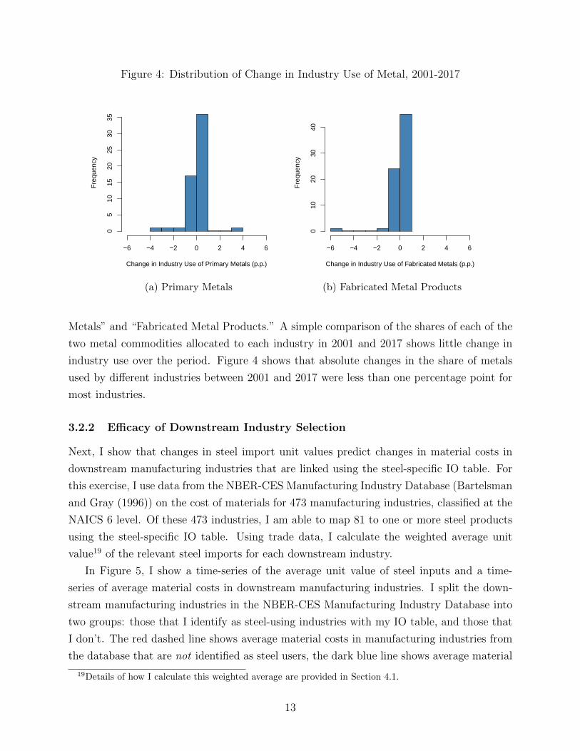
Figure 4: Distribution of Change in Industry Use of Metal, 2001-2017

Change in Industry Use of Primary Metals (p.p.)

Fre

quen

cy

−6 −4 −2 0 2 4 6

05

1015

2025

3035

(a) Primary Metals

Change in Industry Use of Fabricated Metals (p.p.)

Fre

quen

cy

−6 −4 −2 0 2 4 6

010

2030

40

(b) Fabricated Metal Products

Metals” and “Fabricated Metal Products.” A simple comparison of the shares of each of the

two metal commodities allocated to each industry in 2001 and 2017 shows little change in

industry use over the period. Figure 4 shows that absolute changes in the share of metals

used by different industries between 2001 and 2017 were less than one percentage point for

most industries.

3.2.2 Efficacy of Downstream Industry Selection

Next, I show that changes in steel import unit values predict changes in material costs in

downstream manufacturing industries that are linked using the steel-specific IO table. For

this exercise, I use data from the NBER-CES Manufacturing Industry Database (Bartelsman

and Gray (1996)) on the cost of materials for 473 manufacturing industries, classified at the

NAICS 6 level. Of these 473 industries, I am able to map 81 to one or more steel products

using the steel-specific IO table. Using trade data, I calculate the weighted average unit

value19 of the relevant steel imports for each downstream industry.

In Figure 5, I show a time-series of the average unit value of steel inputs and a time-

series of average material costs in downstream manufacturing industries. I split the down-

stream manufacturing industries in the NBER-CES Manufacturing Industry Database into

two groups: those that I identify as steel-using industries with my IO table, and those that

I don’t. The red dashed line shows average material costs in manufacturing industries from

the database that are not identified as steel users, the dark blue line shows average material

19Details of how I calculate this weighted average are provided in Section 4.1.

13

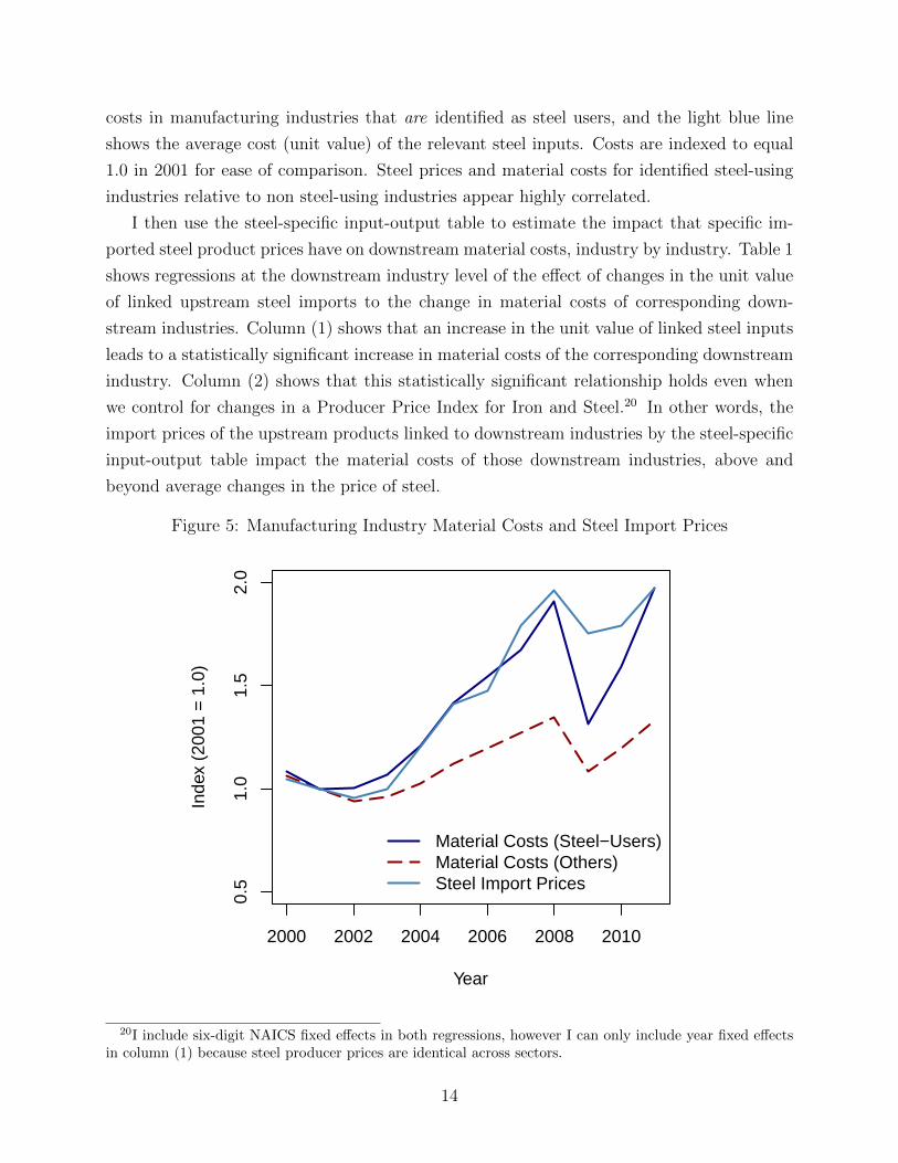
costs in manufacturing industries that are identified as steel users, and the light blue line

shows the average cost (unit value) of the relevant steel inputs. Costs are indexed to equal

1.0 in 2001 for ease of comparison. Steel prices and material costs for identified steel-using

industries relative to non steel-using industries appear highly correlated.

I then use the steel-specific input-output table to estimate the impact that specific im-

ported steel product prices have on downstream material costs, industry by industry. Table 1

shows regressions at the downstream industry level of the effect of changes in the unit value

of linked upstream steel imports to the change in material costs of corresponding down-

stream industries. Column (1) shows that an increase in the unit value of linked steel inputs

leads to a statistically significant increase in material costs of the corresponding downstream

industry. Column (2) shows that this statistically significant relationship holds even when

we control for changes in a Producer Price Index for Iron and Steel.20 In other words, the

import prices of the upstream products linked to downstream industries by the steel-specific

input-output table impact the material costs of those downstream industries, above and

beyond average changes in the price of steel.

Figure 5: Manufacturing Industry Material Costs and Steel Import Prices

2000 2002 2004 2006 2008 2010

0.5

1.0

1.5

2.0

Year

Inde

x (2

001

= 1

.0)

Material Costs (Steel−Users)Material Costs (Others)Steel Import Prices

20I include six-digit NAICS fixed effects in both regressions, however I can only include year fixed effectsin column (1) because steel producer prices are identical across sectors.

14

Table 1: Steel-Import Prices Predict Downstream Material Costs: Industry-Level

(1) (2)∆ Material Costs ∆ Material Costs

∆ Steel Unit Value 0.079 0.078(0.029) (0.029)

∆ PPI Steel 0.574(0.033)

Constant -0.058 -0.023(0.038) (0.040)

Year Fixed Effects Yes No

Sector Fixed Effects Yes YesObservations 888 884

Standard errors in parentheses

Sample years: 2001-2011.

3.2.3 Intensity of Use

Input-output tables typically provide more than just binary indicators of use—they provide

a measure of the intensity of which a downstream industry uses an upstream input. The

exclusion requests I use to formulate the steel-specific IO table provide two key pieces of

information that can be used to proxy for the intensity of an industry’s use of a given

product. First, on each exclusion request, the requesting party must provide the average

annual volume of the 10-digit steel product being requested for exemption consumed between

2015 and 2017. This volume, provided in kilograms, can be converted to dollars using unit

values (dollars per kilogram) of imports of the 10-digit steel import in question. The second

measure of intensity comes from a simple count of the number of downstream industries

that filed an exclusion request for a particular upstream input. This is a coarser measure of

intensity of use, but is useful under the assumption that if a steel input is more important to

or more intensely used by a downstream industry, more parties may file requests to exclude

that input from the tariffs.

To test the strength of these measures of intensity, I compare them to a measure of steel

inputs as a share of a downstream industry’s total input requirements, calculated using the

BEA’s input-output table. Both the quantity measure and the count measure are highly

correlated with the BEA steel-cost share, with correlation coefficients (standard errors) of

0.912 (0.001) and 0.711 (0.02), respectively.

15

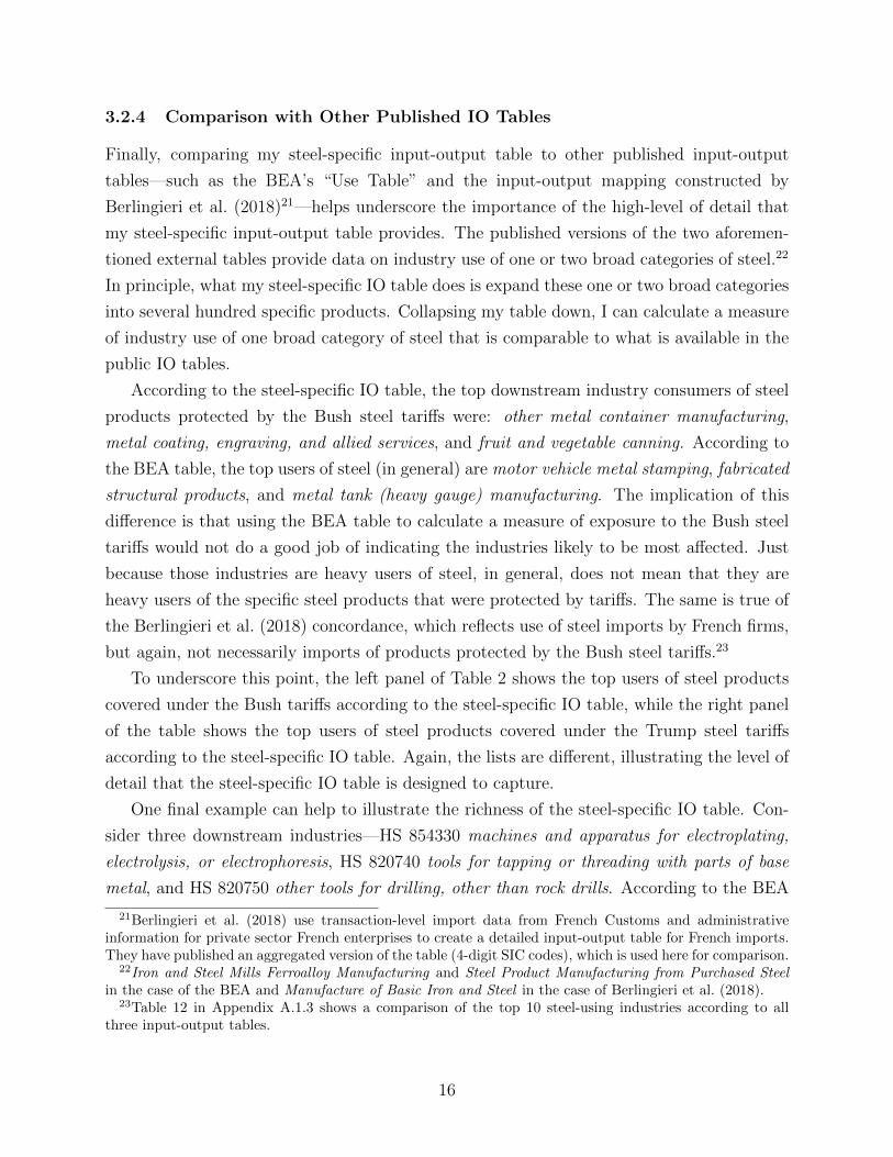
3.2.4 Comparison with Other Published IO Tables

Finally, comparing my steel-specific input-output table to other published input-output

tables—such as the BEA’s “Use Table” and the input-output mapping constructed by

Berlingieri et al. (2018)21—helps underscore the importance of the high-level of detail that

my steel-specific input-output table provides. The published versions of the two aforemen-

tioned external tables provide data on industry use of one or two broad categories of steel.22

In principle, what my steel-specific IO table does is expand these one or two broad categories

into several hundred specific products. Collapsing my table down, I can calculate a measure

of industry use of one broad category of steel that is comparable to what is available in the

public IO tables.

According to the steel-specific IO table, the top downstream industry consumers of steel

products protected by the Bush steel tariffs were: other metal container manufacturing,

metal coating, engraving, and allied services, and fruit and vegetable canning. According to

the BEA table, the top users of steel (in general) are motor vehicle metal stamping, fabricated

structural products, and metal tank (heavy gauge) manufacturing. The implication of this

difference is that using the BEA table to calculate a measure of exposure to the Bush steel

tariffs would not do a good job of indicating the industries likely to be most affected. Just

because those industries are heavy users of steel, in general, does not mean that they are

heavy users of the specific steel products that were protected by tariffs. The same is true of

the Berlingieri et al. (2018) concordance, which reflects use of steel imports by French firms,

but again, not necessarily imports of products protected by the Bush steel tariffs.23

To underscore this point, the left panel of Table 2 shows the top users of steel products

covered under the Bush tariffs according to the steel-specific IO table, while the right panel

of the table shows the top users of steel products covered under the Trump steel tariffs

according to the steel-specific IO table. Again, the lists are different, illustrating the level of

detail that the steel-specific IO table is designed to capture.

One final example can help to illustrate the richness of the steel-specific IO table. Con-

sider three downstream industries—HS 854330 machines and apparatus for electroplating,

electrolysis, or electrophoresis, HS 820740 tools for tapping or threading with parts of base

metal, and HS 820750 other tools for drilling, other than rock drills. According to the BEA

21Berlingieri et al. (2018) use transaction-level import data from French Customs and administrativeinformation for private sector French enterprises to create a detailed input-output table for French imports.They have published an aggregated version of the table (4-digit SIC codes), which is used here for comparison.

22Iron and Steel Mills Ferroalloy Manufacturing and Steel Product Manufacturing from Purchased Steelin the case of the BEA and Manufacture of Basic Iron and Steel in the case of Berlingieri et al. (2018).

23Table 12 in Appendix A.1.3 shows a comparison of the top 10 steel-using industries according to allthree input-output tables.

16

Table 2: Sensitivity of Steel-Specific IO Table

Steel-Specific IO: Bush Tariffs Steel-Specific IO: Trump Tariffs

Other Metal Container Mfg Iron & Steel Pipe and Tube MfgMetal Coating, Engraving, Allied Services New Single-Family Housing ConstructionFruit & Vegetable Canning Other Metal Container MfgOther Motor Vehicle Parts Mfg Steel Wire DrawingOther Transportation Equip. Mfg Other Motor Vehicle Parts MfgSupport Activities: Oil & Gas Metal Coating, Engraving, Allied ServicesFabricated Structural Metal Mfg Fabricated Pipe and Pipe Fitting MfgAll Other Plastics Prod. Mfg Fruit and Vegetable CanningCrane, Hoist, Monorail Sys. Mfg Other Machinery MfgMetal Can Mfg Other Transportation Equipment MfgHardware Mfg Other Fabricated Wire Product Mfg

input-output table, these two downstream industries use similar amounts of steel, with steel

representing between 4 and 5 percent of total costs in each of the three industries. According

to my steel-specific IO table, however, these two industries use very different types of steel,

and as a result, faced different tariff rates on their inputs. In Table 3, I show that HS 854330

is associated with five upstream steel inputs and faced an average increase in steel tariff rate

of 15.5 percent as a result of the Bush steel tariffs. HS 820740 and HS 820750, on the other

hand, are associated with two and one upstream steel inputs, respectively. These industries

faced much larger changes in their average steel tariff rates, at 27.9 and 29.2 percent, respec-

tively. It is this variation that I will leverage in my empirical analysis, that I would not be

able to do using a more aggregated input-output table.

Table 3: Example Demonstrating Richness of Steel-Specific IO Table

HS 854330 HS 820740 HS 82075072139900 72286010 72286010

Steel-Specific IO 72210000 72288000Inputs 72230090

7227906072287030

BEA Steel Cost Share24 4.6 % 4.8 % 4.8%∆ Average Tariff25 15.5 % 27.9 % 29.2 %

4 Estimation Strategy and Threats to Identification

In this section, I discuss the empirical strategy that I use to estimate the effect of tariffs

on upstream steel inputs on the downstream industries that use them. Using the new steel-

specific input-output table described in Section 3, I leverage variation in steel tariff rates faced

by downstream users in 2002-2003 to causally estimate the impact of changes in those rates on

downstream industries. Estimation of these effects is carried out dynamically, providing new

17

evidence about the long-term effects of tariffs on upstream inputs on downstream industries.

4.1 Construction of Downstream Variables

Using the steel-specific input-output table, I construct the key dependent variable of interest:

τd,y—the average statutory tariff rate on steel inputs faced by downstream industry d in year

y. To see how this variable is constructed, consider a downstream industry d that has N

associated upstream steel inputs, which faced tariffs (τ1,y,..., τN,y), respectively, in year y.

The average tariff rate faced by downstream industry d is given by:

τd,y =N∑u=1

ωuτu,y

where ωu is the share of consumption of upstream input u:

ωu =puQu,d∑Nu=1 puQu,d

.

The share of consumption of the upstream inputs is calculated using the average consumption

in kilograms of an upstream product u by a firm in downstream industry d, Qu,d. This

quantity is provided on the exclusion request for each individual firm requesting an exclusion

for product u, and I take the average for all firms in downstream industry d. I convert this

volume to a dollar value using the average (across all countries) unit value of product u from

trade flows data in 2001.26 I use the same weights to construct several control variables,

including a measure of downstream industry’s pre-tariff (2001) exposure to the tariffs,27 and

a measure of the percent of an industry’s steel inputs that cannot be produced in the United

States.28

Due to the different inputs used by different downstream industries, there is substantial

variation in the steel tariff rates those industries faced. This variation, shown in Figure 6, is

the basis for the empirical estimation of the impact that tariffs on upstream inputs have on

downstream industries.

26Trade flows data are simply Customs data, downloaded from the U.S. ITC.27This variable is calculated as the average share of the downstream industry’s imported steel inputs that

come from countries that were not exempt from the Bush tariffs. For example, suppose downstream industryd uses two upstream steel inputs, i and j, in equal proportions. Of total U.S. imports of industry i, 50 percentcame from non-exempt countries in 2001. For input j, 25 percent came from non-exempt countries in 2001.For this industry, I calculate pre-tariff exposure to be: ηd = 1

2 (0.5 + 0.25) = 0.375.28A variable I take from the exclusion requests.

18

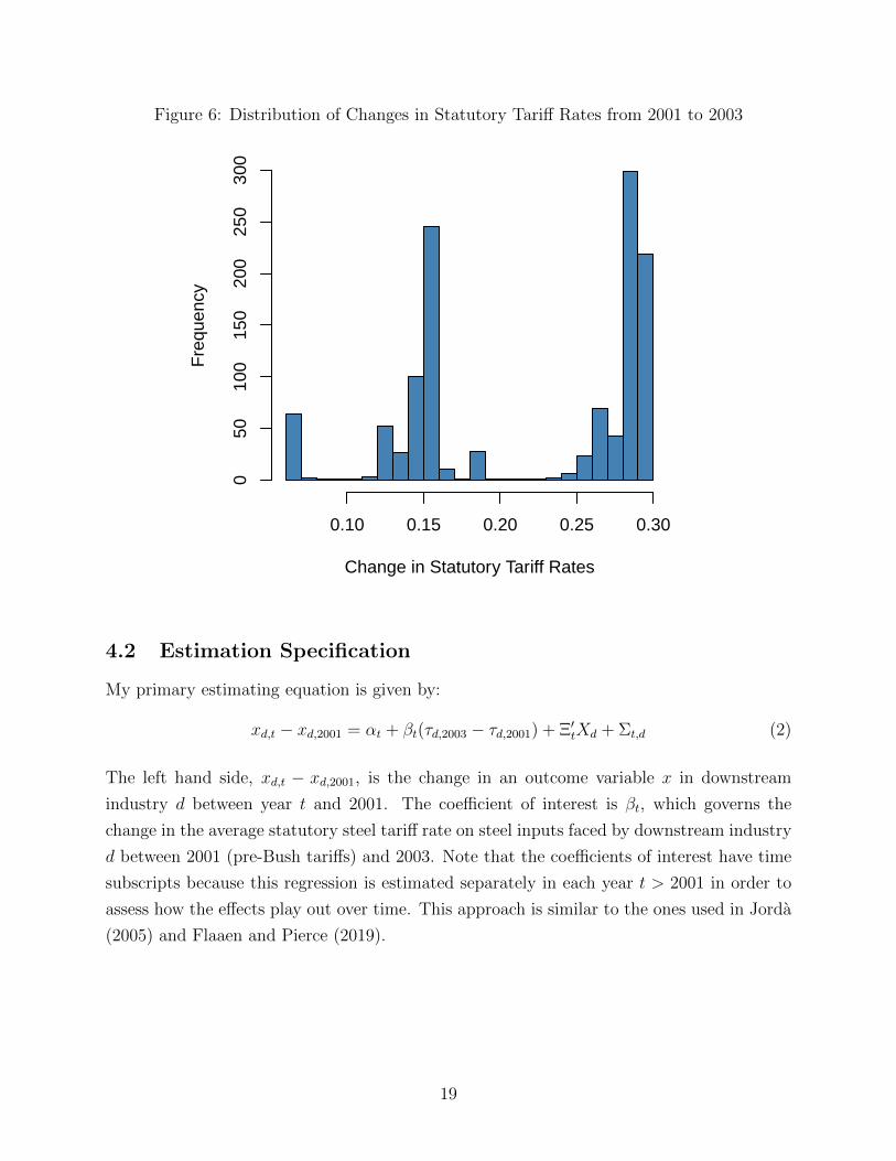
Figure 6: Distribution of Changes in Statutory Tariff Rates from 2001 to 2003

Change in Statutory Tariff Rates

Fre

quen

cy

0.10 0.15 0.20 0.25 0.30

050

100

150

200

250

300

4.2 Estimation Specification

My primary estimating equation is given by:

xd,t − xd,2001 = αt + βt(τd,2003 − τd,2001) + Ξ′tXd + Σt,d (2)

The left hand side, xd,t − xd,2001, is the change in an outcome variable x in downstream

industry d between year t and 2001. The coefficient of interest is βt, which governs the

change in the average statutory steel tariff rate on steel inputs faced by downstream industry

d between 2001 (pre-Bush tariffs) and 2003. Note that the coefficients of interest have time

subscripts because this regression is estimated separately in each year t > 2001 in order to

assess how the effects play out over time. This approach is similar to the ones used in Jorda

(2005) and Flaaen and Pierce (2019).

19

4.3 Threats to Identification

While focusing solely on the downstream impacts of upstream tariffs eliminates many po-

tential threats to identification,29 Gawande et al. (2012) and Bown et al. (2020) point out

several sources of endogeneity that can thwart identification of the negative impacts of tar-

iffs along supply chains. First, because tariffs on upstream products have the potential to

hurt downstream industries, there may be counter-lobbying by downstream firms, especially

those that stand to lose a lot from upstream protection. To the extent that counter-lobbying

efforts are successful, some of the negative impacts of the tariffs will fail to materialize in

the data. In the case of the Bush steel tariffs, there is some evidence to suggest that these

concerns can be at least partially alleviated. A document published by USTR following the

announcement of then tariffs indicates that the level of tariffs that were levied on all but

one category of steel product (stainless steel bar) were equal to or higher than the level

recommended by the majority of ITC commissioners.30 In other words, if there was lobbying

by downstream industries to reduce tariff rates relative to ITC recommendations, it appears

to have been unsuccessful.

There is anecdotal evidence to support this story as well. According to an article pub-

lished by the Wall Street Journal31 on March 6, 2002 (days after the tariffs were announced):

For months, trade analysts and even some administration officials had thought

the president would impose only very limited tariffs. In the months-long lobbying

war that preceded Tuesday’s decision, those who opposed high tariffs appeared

to have the upper hand. Steel-using manufacturers and port owners gained the

administration’s ear, arguing that tariffs would cost far more jobs than they

saved... But in the final days, Bush advisers say, the White House came under

intense pressure from the steel unions, the big steel companies, and perhaps most

important, lawmakers from steel states. The unions held a mass rally outside the

White House last Thursday, while steel-state legislators made their case in the

Oval Office. Officials say Mr. Bush and his advisers most feared a possible

backlash among voters in the “rust belt,” as well as erosion of support for Mr.

Bush’s other trade objectives in Congress... Sharply limited tariffs would have

let the weakest coke-and-iron-ore steelmakers die and helped the strongest to

29When looking at the own-industry impact of protection, an industry’s need for protection is likelycorrelated with its performance. Downstream industries, however, are more likely to be collateral damage—they are not specifically targeted.

30http://lobby.la.psu.edu/_107th/097_Steel_Safeguard/Agency_Activities/USTR/USTR_Bush_

decides_on_safeguards.pdf31https://www.wsj.com/articles/SB101533904883100680

20

Table 4: Testing for Pre-Trends

(1) (2) (3)∆ Export Share (98-01) ∆ Log Exports (98-01) ∆ Log Export Price (98-01)

∆ statutory tariff 0.023 0.382 0.223(0.024) (0.245) (0.655)

Standard errors in parentheses∗ p < 0.05, ∗∗ p < 0.01, ∗∗∗ p < 0.001

grow and become more efficient competitors of mini-mills. Instead, Mr. Bush

extended help to the steel industry across the board.

In other words, the will of the downstream lobby appears to have been overridden by other

political concerns.

A second potential source of endogeneity is that there is an omitted variable that is

correlated with both the tariff on upstream inputs faced by a downstream industry, and the

downstream industry outcome. For example, suppose foreign input suppliers experience a

positive productivity shock that leads to an influx of imported inputs. On one hand, the

influx of imported inputs might induce a higher tariff rate on those inputs as domestic input

suppliers demand a greater level of protection. On the other hand, the influx could also boost

domestic downstream production, leading to a positive correlation between downstream

outcomes and input tariffs. Similarly, a productivity shock in the domestic downstream

industry could lead to an influx of imported inputs that leads to a higher tariff rate. I test

for endogeneity of this form by regressing changes in downstream industry outcomes leading

up to the tariffs on the tariff rates those industries faced. Specifically, I run the following:

∆yd,1998−2001 = α + β(τd,2003 − τd,2001) + εd (3)

Where y is the change in the downstream variable of interest between 1998 and 2001.

The results are reported in Table 4. There is not a statistically significant relationship for

any of the outcome variables of interest, suggesting downstream industries that faced higher

upstream tariffs were not on differential trajectories prior to those tariffs being implemented.

The dynamic regression specification that I employ throughout Section 5 similarly shows

that there are no apparent pre-trends.32 Together, this evidence assuages concerns about

the presence of endogeneity in the form of an omitted variable.

Finally, it is worth noting that any of the sources of endogeneity discussed will likely bias

my results upward, making it harder to identify negative impacts of tariffs on downstream

industries.32Lake and Liu (2021) similarly highlight the absence of pre-trends between 1998 and 2000 in their

difference-in-differences specification to show that the parallel trends assumption holds.

21

5 The Downstream Impact of Steel Tariffs

In this section, I describe my empirical findings on the impact of steel tariffs on downstream

industries. Unless otherwise noted, results are estimated using the dynamic specification in

equation 2, and results are shown for two samples: all downstream industries (dark blue

line), and steel-intensive industries (red line, defined as industries for which steel constitutes

an above-median share of costs).33

5.1 Downstream Export Market

I first consider the impact of the tariffs on the export performance of downstream industries.

I consider both the log level of exports (values and quantities), log export prices, and then

the U.S. share of global exports—a measure of U.S. market share. Figure 7a shows that

downstream industries that faced relatively high steel tariffs saw relatively large declines in

export values (prices times quantities). Specifically, a one percentage point increase in an

industry’s steel tariff rate is associated with a peak decline of one percent in exports relative

to pre-tariff levels (2 percent for steel-intensive industries).34 Exports remain dampened for

6 years after the tariffs are removed for all industries, and for even longer for steel-intensive

industries.

Figures 7c and 7d show that relative declines in export values were due to both lower

export quantities and prices. The price (unit-value) and quantity data available from U.S.

Customs is notoriously noisy, so I show results that are smoothed using two-year rolling

regressions. For transparency, the raw results are in the Appendix. Exported quantities

decline upon impact of the tariffs and remain dampened, while export prices remain flat

on impact before eventually declining. That sectors that faced higher input tariffs saw

lower export prices and quantities suggests that foreign consumers reallocate away from

U.S. production, lowering prices in those sectors. (See Section 5.4 for further discussion).

Fajgelbaum et al. (2020) also find that sector-level export prices fell with retaliatory tariffs

during the Trump trade wars, as retaliatory tariffs induced a similar reallocation of foreign

demand away from the U.S. In all four panels of Figure 7, note the absence of apparent

pre-trends.

33I categorize industries using cost-shares calculated from the BEA total requirements table, but I getsimilar results using measures of intensity discussed in Section 3.2.3.

34Handley et al. (2020) study the impact of the Trump tariffs on downstream industry export values.While the magnitude I estimate cannot be compared directly with the theirs due to the use of a differentindependent variable (they use a measure of industry exposure to the tariffs), the direction is consistent withtheir findings.

22

Figure 7: Effect of Higher Statutory Rates on Downstream Exports

−4

−2

02

Year(tick at start of period)

Res

pons

e to

1 p

.p. I

ncre

ase

in S

tatu

tory

Rat

e

ResponseTariff Period 90% CI

All DownstreamAbove Median Intensity

1997 2001 2005 2009 2013

(a) Export Values−

0.3

−0.

2−

0.1

0.0

0.1

Year(tick at start of period)

Res

pons

e to

1 p

.p. I

ncre

ase

in S

tatu

tory

Rat

e

ResponseTariff Period 90% CI

All DownstreamAbove Median Intensity

1997 2001 2005 2009 2013

(b) Export Share

−6

−4

−2

02

Year(tick at start of period)

Res

pons

e to

1 p

.p. I

ncre

ase

in S

tatu

tory

Rat

e

ResponseTariff Period 90% CI

All DownstreamAbove Median Intensity

1998 2000 2002 2004 2006 2008 2010 2012 2014

(c) Export Quantities

−3

−2

−1

01

23

Year(tick at start of period)

Res

pons

e to

1 p

.p. I

ncre

ase

in S

tatu

tory

Rat

e

ResponseTariff Period 90% CI

All DownstreamAbove Median Intensity

1998 2000 2002 2004 2006 2008 2010 2012 2014

(d) Export Prices

Figure 7b shows the response of the U.S. share of global exports in downstream industries

to the tariffs—a measure of the industry’s global competitiveness or global market share.

For downstream industries that faced relatively high steel tariffs, export shares exhibited

a sharp decline during the period in which the tariffs are in place and remain depressed

relative to pre-tariff levels for at least 8 years after the tariffs are removed. To put the

magnitude of the estimated impact into perspective, shifting an industry from the 25th to

the 75th percentile in terms of the change in upstream tariff it faces between 2001 and 2003

23

(a swing of 13.5 percentage points) results in a relative decline in global market share of

0.9 percentage points per year (on average) overall, and 1.9 percentage points per year for

steel-intensive industries.

5.2 Reconfiguration of Global Trade Flows

The notion that temporary tariffs can have persistent downstream effects on the competitive-

ness of U.S. exports implies that there is a reconfiguration of downstream global trade flows

in response to the tariffs that does not revert back once the tariffs are lifted. To test this, I

use data on exports of the top 25 non-U.S. exporters of the relevant downstream products.

I run the analogous specification to equation 2, but replace the dependent variable with the

change in export share in downstream industry d in country j between year t and 2001.

xdj,t − xdj,2001 = αt + βt(τd,2003 − τd,2001) + Ξ′tXd + Σt,d (4)

Of the top 25 exporters I find that higher tariffs in a U.S downstream industry lead to a sig-

nificant increase in global market share in those industries for Germany, Japan, and France.

Regression results for these three countries are shown in Figure 8. Upon implementation of

the tariffs in the United States, foreign market shares in industries that faced relatively high

tariffs in the U.S. saw relative increases, especially for steel-intensive industries. German

market shares exhibited the strongest response, followed by Japan and France. Notably,

prior to the tariffs being enacted in the U.S., Germany, Japan and France were the second,

third, and fourth largest exporters (in that order) of products in these downstream industries

(behind the United States). As was the case in the U.S. export market, foreign market share

responses to the steel tariffs are highly persistent.35

5.3 Downstream Domestic Outcomes

Lastly, I consider the impact of upstream tariffs on domestic downstream production and em-

ployment. Data on domestic production for domestic consumption (i.e., excluding exports)

are not readily available, so instead I estimate the response of U.S. imports of downstream

industry products.36 Intuitively a relative increase in imports for products that faced higher

35Note that because I am comparing the relative outcomes of U.S. industries that faced different upstreamtariff rates and because I am estimating the results separately in each year (i.e., my regressions have timefixed effects), exchange rates will not be a factor in these results.

36In the Appendix I show results using a variable created using data on the value of shipments from theNBER CES Manufacturing Database, less industry exports, but this is a relatively noisy measure since thetwo data sources are measured using different industry classifications. The results are consistent, but arenot measured with precision.

24

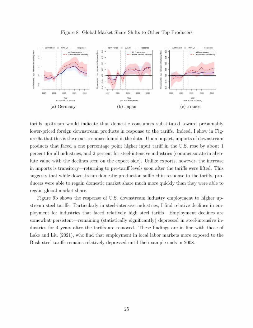
Figure 8: Global Market Share Shifts to Other Top Producers−

0.1

0.0

0.1

0.2

Year(tick at start of period)

Res

pons

e to

1 p

.p. I

ncre

ase

in S

tatu

tory

Rat

e

ResponseTariff Period 90% CI

All DownstreamAbove Median Intensity

1997 2001 2005 2009 2013

(a) Germany−

0.10

−0.

050.

000.

050.

100.

150.

20

Year(tick at start of period)

Res

pons

e to

1 p

.p. I

ncre

ase

in S

tatu

tory

Rat

e

ResponseTariff Period 90% CI

All DownstreamAbove Median Intensity

1997 2001 2005 2009 2013

(b) Japan

−0.

10−

0.05

0.00

0.05

0.10

0.15

0.20

Year(tick at start of period)

Res

pons

e to

1 p

.p. I

ncre

ase

in S

tatu

tory

Rat

e

ResponseTariff Period 90% CI

All DownstreamAbove Median Intensity

1997 2001 2005 2009 2013

(c) France

tariffs upstream would indicate that domestic consumers substituted toward presumably

lower-priced foreign downstream products in response to the tariffs. Indeed, I show in Fig-

ure 9a that this is the exact response found in the data. Upon impact, imports of downstream

products that faced a one percentage point higher input tariff in the U.S. rose by about 1

percent for all industries, and 2 percent for steel-intensive industries (commensurate in abso-

lute value with the declines seen on the export side). Unlike exports, however, the increase

in imports is transitory—returning to pre-tariff levels soon after the tariffs were lifted. This

suggests that while downstream domestic production suffered in response to the tariffs, pro-

ducers were able to regain domestic market share much more quickly than they were able to

regain global market share.

Figure 9b shows the response of U.S. downstream industry employment to higher up-

stream steel tariffs. Particularly in steel-intensive industries, I find relative declines in em-

ployment for industries that faced relatively high steel tariffs. Employment declines are

somewhat persistent—remaining (statistically significantly) depressed in steel-intensive in-

dustries for 4 years after the tariffs are removed. These findings are in line with those of

Lake and Liu (2021), who find that employment in local labor markets more exposed to the

Bush steel tariffs remains relatively depressed until their sample ends in 2008.

25

Figure 9: Effect of Tariffs on Imports and Employment

−4

−2

02

4

Year(tick at start of period)

Res

pons

e to

1 p

.p. I

ncre

ase

in S

tatu

tory

Rat

e

ResponseTariff Period 90% CI

All DownstreamAbove Median Intensity

1997 2001 2005 2009 2013

(a) U.S. Import Quantities

−1.

5−

1.0

−0.

50.

00.

51.

01.

5

Year(tick at start of period)

Res

pons

e to

1 p

.p. I

ncre

ase

in S

tatu

tory

Rat

e

ResponseTariff Period 90% CI

All DownstreamAbove Median Intensity

1997 1999 2001 2003 2005 2007 2009 2011

(b) Employment

5.4 Discussion of Empirical Results

The results presented in Sections 5.1 through 5.3 can be summarized by three main findings:

(1) higher tariffs on steel inputs have a persistent negative impact on exports in downstream

industries; (2) global market share in downstream industries that faced higher steel tariffs

shifted to other top exporting countries; and (3) higher input tariffs have a negative impact

on downstream domestic production, but this impact is more transitory. In Figures 10 and

11, I depict a simple conceptual framework to interpret the short- and long-run effects,

respectively. The intuitions from these graphs guide my reduced-form welfare calculations

in Section 6 and the full structural model in Section 7. A unified conceptual framework can

help explain these findings.

In the short run, on the export side, the data showed sharp relative declines in downstream

exported quantities accompanied by little to no change in export prices. This suggests that

U.S. downstream exporters are facing a relatively elastic foreign demand curve, as depicted

in Figure 10b. My findings on the domestic side are the opposite: tariffs induce little change

in quantities and only a small (albeit imprecisely measured) increase in prices. This suggests

that domestic demand is fairly inelastic, as shown in Figure 10a in contrast to its foreign

counterpart.

Once the tariffs are lifted, I find that domestic prices and outcomes bounce back relatively

quickly; in other words, the U.S. supply curve appears to revert to its pre-tariff location. In

the export market, however, persistent declines in both export prices and quantities imply an

26

Figure 10: Contemporaneous Effect of Steel Tariffs on Downstream Industries

Q

P

S

D

S′

p0

p1

q0q1

(a) Domestic Market

X

P

SUS

S′US

DROWp0

x0x1

(b) Export Market

inward shift of the foreign demand curve (see Figure 11b). Consistent with this explanation,

Section 5.2 showed that other top exporters of downstream products—Germany, Japan,

and France—took over the forfeited U.S. market share, explaining the ensuing reduction in

demand for U.S. products. The persistent nature of this dampened foreign demand can be

explained by the presence of relationship-specific sunk costs. Intuitively, if foreign buyers

that were purchasing from the U.S. switch to a cheaper source (e.g. Germany) when the

tariffs are implemented, it may not be worth it for all buyers to return to the U.S. once

the tariffs are removed if there are high enough sunk costs associated with doing so. This

graphical analysis will guide my reduced form estimation of the welfare impacts of the Bush

steel tariffs, presented in the next section, and the intuition will carry through the structural

model presented in Section 7.

Figure 11: Persistent Effects of Steel Tariffs on Downstream Industries

Q

P

S

D

p0 = p1

q0 = q1

(a) Domestic Market

X

P

SUS

DROW

D′ROW

p0

p1

x0x1

(b) Export Market

27

6 Reduced Form Estimates of Welfare Impacts

The welfare impacts of steel tariffs will materialize both in the market for imported steel—

through changes in consumer surplus, terms of trade, and tariff revenue—and in the market

for downstream products. I focus on downstream welfare impacts in the form of producer

surplus in the market for exports. It is here that I find the strongest impact in my empirical

results, and also where I find that persistence is most likely to be a factor (as per the

discussion in Section 5.4). In this section, I estimate the aggregate welfare impacts of the

steel tariffs, both in the steel sector (contemporaneously) and in downstream industries

(dynamically). I do this by assuming fairly general forms for the downstream industry

export supply curve and the steel import demand curve, empirically estimating the U.S.

elasticities of downstream export supply and steel import demand, respectively, and then

using reduced form evidence to calculate changes in aggregate surplus due to the tariffs

between 2002 and 2009.

6.1 Downstream Industries

In the downstream export market, changes in welfare will be represented by changes in

aggregate producer surplus, or aggregate profit.37 In general terms, consider a policy change

that lowers prices in a sector, d, from pd,t to pd,t+k. If we assume that production is allocated

optimally across firms,38 the ensuing change in producer surplus will be given by:

∆PSd,t+k = Πd(pt)− Πd(pt+k) = −∫ pt

pt+k

qd,t+k(s)ds

Making one further assumption, that downstream industry supply curves are upward sloping

and take the (inverse) form:

pt = aqσt , (5)

where a is a marginal cost shifter and σ is the elasticity of supply, I rewrite the formula for

producer surplus as:

37The conventional method for measuring policy-induced changes in welfare in a partial equilibrium modelis to estimate changes in aggregate surplus—the net of producer surplus, consumer surplus, and tax revenue.In this case, consumer surplus accrues in the foreign market, and there is no tax revenue downstream.

38That is, marginal costs of production are equated across firms in an industry.

28

∆PSd,t+k =

∫ pt

pt+k

(ap)1σ = qtp

σ+1t

σ

σ + 1

[1− (∆ ln pt+k + 1)

σ+1σ

](6)

For the scenario in question, I estimate σ, the elasticity of supply for downstream U.S.

exporters. I observe pd,t and qd,t, pre-tariff export prices and quantities; and using the

estimate of σ and dynamic estimates of changes in quantities due to the tariffs, we can

calculate the change in downstream producer surplus in each year due to the steel tariffs.

Estimating the Elasticity of Supply, σ

Starting with the production function (5) and taking log-differences yields:

∆ ln pt+k = σ∆ ln qt+k. (7)

In this case, ∆ ln pt+k is the change in U.S. export prices between periods t and t + k,

and ∆ ln qt+k is the change in export quantities during the same period. Of course, the

endogeneity of prices and quantities precludes us from credibly running a regression of the

form above. We can, however, instrument for ∆ ln qt+k with an appropriate exogenous foreign

demand shock to get an unbiased estimate of σ.

I construct a foreign demand shock as follows. First, I consider the top 10 sources of

U.S. exports of downstream products.39 Let mid,t be imports of downstream product d by

country i in year t from all sources excluding the United States and define Md,t =∑

i mid,t.

Following Mayer et al. (2016), in each year, t, I calculate a first difference as:

∆Md,t = (Md,t − Md,t−1)/(0.5Md,t + 0.5Md,t−1)

This measure is useful because it preserves observations when Md,t switches from 0 to a

positive number and is bounded between -2 and 2. ∆Md,t, then, represents increases in

“world” demand (as represented by the top 10 U.S. buyers), and can be used to instrument

for ∆ ln qt+k in equation 7 to estimate σ.

Results are shown in Table 5. I estimate an inverse elasticity of export supply of σ = 0.29,

suggesting export supply is fairly elastic. This estimate is in line with similar estimates from

the literature, for example Romalis (2007) who estimates a value between 0.24 and 0.52. I

use the estimate from column (1), which covers sample years 1995-2001 (pre-tariff), but the

estimate is robust to sample selection.

39Canada, Mexico, Japan, Germany, United Kingdom, France, Brazil, China, South Korea, Netherlands

29

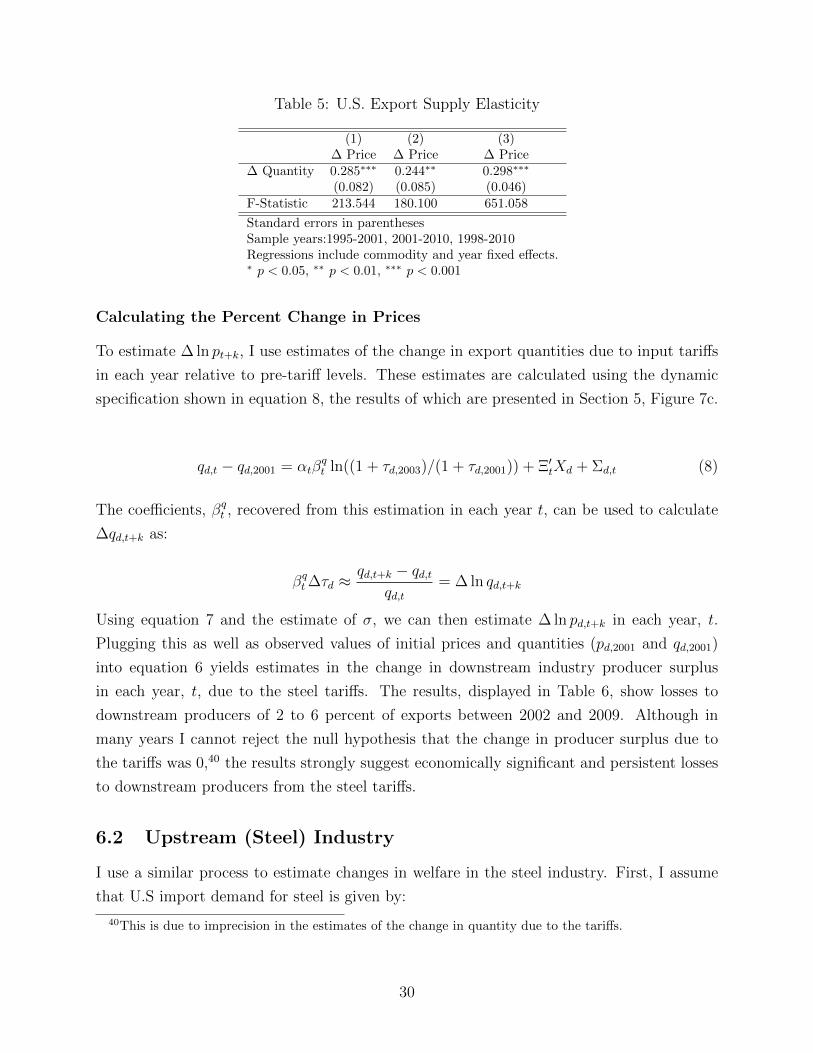
Table 5: U.S. Export Supply Elasticity

(1) (2) (3)∆ Price ∆ Price ∆ Price

∆ Quantity 0.285∗∗∗ 0.244∗∗ 0.298∗∗∗

(0.082) (0.085) (0.046)F-Statistic 213.544 180.100 651.058

Standard errors in parenthesesSample years:1995-2001, 2001-2010, 1998-2010Regressions include commodity and year fixed effects.∗ p < 0.05, ∗∗ p < 0.01, ∗∗∗ p < 0.001

Calculating the Percent Change in Prices

To estimate ∆ ln pt+k, I use estimates of the change in export quantities due to input tariffs

in each year relative to pre-tariff levels. These estimates are calculated using the dynamic

specification shown in equation 8, the results of which are presented in Section 5, Figure 7c.

qd,t − qd,2001 = αtβqt ln((1 + τd,2003)/(1 + τd,2001)) + Ξ′tXd + Σd,t (8)

The coefficients, βqt , recovered from this estimation in each year t, can be used to calculate

∆qd,t+k as:

βqt∆τd ≈qd,t+k − qd,t

qd,t= ∆ ln qd,t+k

Using equation 7 and the estimate of σ, we can then estimate ∆ ln pd,t+k in each year, t.

Plugging this as well as observed values of initial prices and quantities (pd,2001 and qd,2001)

into equation 6 yields estimates in the change in downstream industry producer surplus

in each year, t, due to the steel tariffs. The results, displayed in Table 6, show losses to

downstream producers of 2 to 6 percent of exports between 2002 and 2009. Although in

many years I cannot reject the null hypothesis that the change in producer surplus due to

the tariffs was 0,40 the results strongly suggest economically significant and persistent losses

to downstream producers from the steel tariffs.

6.2 Upstream (Steel) Industry

I use a similar process to estimate changes in welfare in the steel industry. First, I assume

that U.S import demand for steel is given by:

40This is due to imprecision in the estimates of the change in quantity due to the tariffs.

30

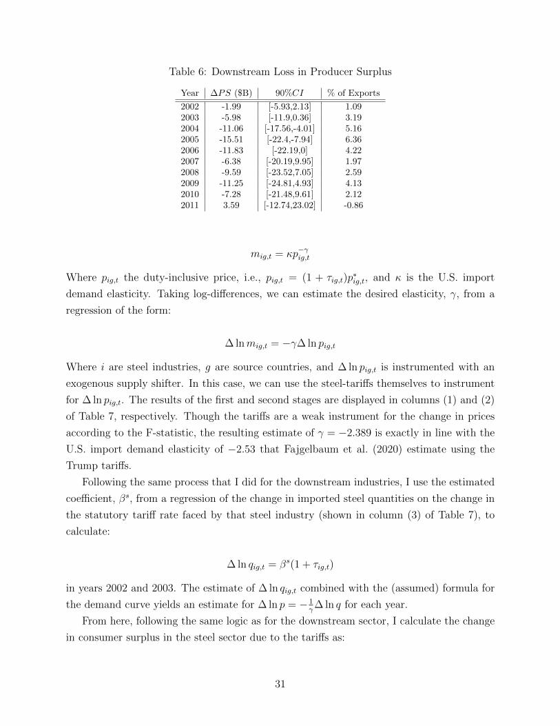
Table 6: Downstream Loss in Producer Surplus

Year ∆PS ($B) 90%CI % of Exports

2002 -1.99 [-5.93,2.13] 1.092003 -5.98 [-11.9,0.36] 3.192004 -11.06 [-17.56,-4.01] 5.162005 -15.51 [-22.4,-7.94] 6.362006 -11.83 [-22.19,0] 4.222007 -6.38 [-20.19,9.95] 1.972008 -9.59 [-23.52,7.05] 2.592009 -11.25 [-24.81,4.93] 4.132010 -7.28 [-21.48,9.61] 2.122011 3.59 [-12.74,23.02] -0.86

mig,t = κp−γig,t

Where pig,t the duty-inclusive price, i.e., pig,t = (1 + τig,t)p∗ig,t, and κ is the U.S. import

demand elasticity. Taking log-differences, we can estimate the desired elasticity, γ, from a

regression of the form:

∆ lnmig,t = −γ∆ ln pig,t

Where i are steel industries, g are source countries, and ∆ ln pig,t is instrumented with an

exogenous supply shifter. In this case, we can use the steel-tariffs themselves to instrument

for ∆ ln pig,t. The results of the first and second stages are displayed in columns (1) and (2)

of Table 7, respectively. Though the tariffs are a weak instrument for the change in prices

according to the F-statistic, the resulting estimate of γ = −2.389 is exactly in line with the

U.S. import demand elasticity of −2.53 that Fajgelbaum et al. (2020) estimate using the

Trump tariffs.

Following the same process that I did for the downstream industries, I use the estimated

coefficient, βs, from a regression of the change in imported steel quantities on the change in

the statutory tariff rate faced by that steel industry (shown in column (3) of Table 7), to

calculate:

∆ ln qig,t = βs(1 + τig,t)

in years 2002 and 2003. The estimate of ∆ ln qig,t combined with the (assumed) formula for

the demand curve yields an estimate for ∆ ln p = − 1γ∆ ln q for each year.

From here, following the same logic as for the downstream sector, I calculate the change

in consumer surplus in the steel sector due to the tariffs as:

31

Table 7: U.S. Import Demand Elasticity

(1) (2) (3)∆ Log Duty-Inclusive Price ∆ Log Quantity ∆ Log Quantity

∆ Log (1+τ) 0.737∗ -4.598∗∗

(0.295) (1.443)

∆ Log Duty-Inclusive Price -2.389∗

(1.090)

Constant 0.047 0.420(0.053) (0.223)

F-Statistic 5.835

Standard errors in parenthesesSample years: 2002-2003Regressions include country-year fixed effects.∗ p < 0.05, ∗∗ p < 0.01, ∗∗∗ p < 0.001

∆CSd,t+k = qtpt

(1

1− γ

)[1− (1 + ∆pt+k)

1−γ]The resulting estimates, shown in the third column of Table 8, also include changes tariff

revenue earned due to the tariffs in the two years in which the tariffs were in place.

6.3 Overall Change in Welfare

Combining estimates of changes in welfare in the downstream sectors with changes in the

steel sector, I calculate the overall change in welfare due to the steel tariffs, relative to pre-

tariff levels, in each year. The results are shown in Table 8. I find that welfare losses amount

to between 1 and 6 percent of exports in each year. Losses are primarily concentrated in

the downstream sector, though persistent declines in the downstream sector may have had a

continuing negative impact upstream as well (in most years, I cannot reject the null hypoth-

esis of 0 change in welfare in the upstream sector). More important than the magnitudes

estimated in each year is the fact that welfare losses accrue for years after the tariffs were

removed, something that conventional methods for evaluating the impacts of such a policy

traditionally miss. A comprehensive estimate of the welfare impacts of an input tariff will be

substantially underestimated if the downstream dynamic impacts are not taken into account.

In the next section, I show that welfare losses estimated using a full structural model are in

line with these partial equilibrium calculations.

32

Table 8: Overall Welfare Loss from 2002-2003 Steel Tariffs

Year Downstream ($B) Upstream ($B) Total ($B) Total % of Exports

2002 -1.99* -0.51 -2.49* 1.37*2003 -5.98* -0.88 -6.86* 3.66*2004 -11.06* -0.37* -11.42* 5.33*2005 -15.51* -0.18 -15.69* 6.43*2006 -11.83* -0.52 -12.35* 4.41*2007 -6.38 -0.38 -6.76 2.092008 -9.59 0.13 -9.46 2.552009 -11.25 -0.52 -11.77 4.32

A * indicates that result is statistically significant with a 90 percent confidence interval.

7 A Structural Dynamic Model

In this section, I present a dynamic model of trade that features relationship-specific sunk

costs of exporting. I use the model first to show that the presence of sunk costs can generate

a persistent response of downstream exports to a temporary input tariff that is consistent

with the patterns that I find in the data. I then use the model to evaluate the aggregate

welfare implications of a temporary input tariff shock.

7.1 Overview

The model features two asymmetric countries (Home and Foreign), each with three sectors:

an (Armington) steel sector, which uses labor to create tradable steel products; a down-

stream manufacturing sector, which uses labor and a composite of home and foreign steel to

produce a (differentiated) tradable consumption good; and an outside sector that produces

a homogeneous consumption good that is freely traded. Governments can place tariffs on

steel imports to support the domestic steel industry and generate tariff revenue. Households

provide labor and earn wages in all three producing sectors, and derive utility from the con-

sumption of a Cobb-Douglas aggregate of downstream manufactured goods and the outside

sector good.

The downstream manufacturing industry is modeled in the spirit of Melitz (2003). The

industry features a large number of monopolistically competitive establishments. As in

Melitz (2003), establishments in the downstream sector must pay a fixed cost in order to

export goods. As a result, not all establishments will find it profitable to sell in the foreign

market. In each period, a mass of existing establishments are distributed over productivity

and export status. Idiosyncratic shocks to productivity and fixed export costs generate

movements of establishments into and out of the domestic and export markets. There is

33

free entry, and new establishments are created by incurring a fixed entry cost. The key

feature of the model is that there is a sunk cost associated with entering the export market:

specifically, the fixed cost of starting to export differs from the cost of continuing to export.

Seminal work by Baldwin (1988), Baldwin and Krugman (1989), and Dixit (1989) showed

that the presence of such a sunk cost generates hysteresis in export dynamics in response to

temporary shocks.

Steel tariffs levied by the home country force some downstream manufacturing firms to

exit the export market, as higher input costs render exporting unprofitable. The opposite

occurs in the foreign country, where producers find it more profitable to enter. As soon as

the tariffs are lifted, domestic steel input prices return to pre-tariff levels, but due to the

sunk cost that firms face in their initial exporting period, home country exporters cannot

immediately re-join the export market and extra entrants in the foreign country do not

immediately exit. As a result, the economy is slow to converge back to its initial steady

state.

7.2 Set-Up

In this subsection I will describe the model’s basic features. Further details are relegated to

Appendix A.5.

Steel Sector.

Steel production occurs both at home (s) and abroad (ω) using the production technologies:

st = A`t

ωt = A∗`∗t ,

where A is a country-specific productivity parameter. Steel is tradeable, and downstream

goods in each country are produced using a composite of home and foreign steel inputs:

St =[sε−1ε

t + ωε−1ε

t

] εε−1

,

where s is consumption of domestically produced steel, ω is imported steel, and ε is the

elasticity of substitution between home and foreign steel. Steel consumption in the foreign

country is analogous (unless otherwise noted, assume that this is the case going forward).

Foreign variables will be demarcated with an asterisk going forward. Prices of home and

34

foreign steel are given by ps,t and pω,t, respectively. The home government can place a tariff,

τs, on imported steel, so that the price of foreign steel in the home country is given by

(1 + τs)pω,t. The price of the composite steel product is standard:

P St =

[(ps,t)

1−ε + ((1 + τs)pω,t)1−ε] 1

1−ε .

Outside Good Sector.

The outside consumption good is produced (linearly) with labor. The outside good, DO, is

sold in a competitive market and is freely traded across countries. I treat the outside good

as the numeraire and normalize the wage in each country to 1: Wt = W ∗t = 1.41

Households.

Households choose consumption and investment to maximize utility:

VC,0 = max∞∑t=0

βtU(Ct)

subject to the sequence of budget constraints:

PtCt +QtBt ≤ PtWtLt +Bt−1 + PtΠt + PtTt,

where β ∈ (0, 1) is the time discount factor, Ct is consumption of final goods, Qt and Bt

are the price of and quantity of bond holdings, Wt is the real wage rate, Πt are profits from

domestic producers, and Tt is a real lump-sum transfer from the home government to the

households that includes tariff revenue collected in the steel sector. Households have log

utility over consumption of the final good, whose composition is described next.

Final Good Producers.

There is a final good production sector that assembles the consumption good—a Cobb-

Douglas composite of the outside good, DO and the manufactured good, DT :

Dt = DγT,tD

1−γO,t

where DT,t is a CES composite of domestic and foreign tradeable manufactured goods,

yH,t(z, v, x) and yF,t(z, v, x):

41While Demidova and Rodriguez-Clare (2013) argues that the addition of an outside sector to the Melitz(2003) model can affect the welfare implications of changes in iceberg tariffs, as argued in Bagwell and Lee(2020), changes in sector-specific ad valorem tariffs, as I study here, are less likely to generate aggregatewage effects. Therefore, an outside sector seems reasonable in this case.

35

DT =

[1∑

x=0

∫∫yH,t(z, v, x)

θ−1θ ψT,t(z, v, x)dz + yF,t(z, v, x)

θ−1θ ψ∗T,t(z, v, 1)dzdv

] θθ−1

Here, (z, v, x) is a technology triplet that defines downstream firms and will be defined in

the next section, ψT (z, v, x) and ψ∗T (z, v, 1) are the distributions of downstream producers in

the Home country and downstream exporters in the Foreign country, and θ is the elasticity

of substitution among downstream manufactured goods.

Downstream Manufacturing Sector

Downstream good producers are heterogeneous with respect productivity, and therefore, ex-

port status. The set-up of the downstream sector is adapted from Alessandria and Choi

(2014). Incumbent firms have idiosyncratic productivity, z, which follows a first-order

Markov process where a firm’s probability of having productivity z′ in period t+ 1 given it

has productivity z in period t is given by Φ(z′|z). Next-period productivity, z′ is bounded

by z′ ∈ (z, z). Establishments face an exogenous probability of “death” (or exogenous

exit) given by 0 ≤ nd(z) ≤ 1. The survival rate of a firm with productivity z is given by

ns(z) = 1− nd(z).

There is a fixed cost associated with exporting, that depends on the firm’s current export

status. An incumbent exporter in period t must pay the cost f1 in each period to continue

exporting in period t + 1. A firm that is not exporting in period t must pay f0 to start

exporting in period t + 1, where f0 > f1. Thus, it is more costly to start exporting than to

continue exporting. These fixed costs are subject to idiosyncratic shocks, v, drawn in each

period from φv(v).

In each period, producers draw their exporting fixed cost shocks, productivity shocks,

and make a decision about whether to export in the next period. Lastly, entrants pay a fixed

entry cost fE to draw a productivity parameter, z, for the next period from the distribution

φE(z′). Firms in the downstream manufacturing sector are defined by the triplet: technology

(z), fixed cost shock (v), and export status (x). Let j = (z, v, x). In each period, firms choose

current prices, PH,t(j) and P ∗H,t(j); inputs of labor, `T,t(j), and the composite steel product,

sT,t(j); and the next period’s export status. Producers have a Cobb-Douglas production

technology:

yT,t = exp(z)[sT,t(j)

α`T,t(j)1−α]

And producers solve the following Bellman equation:

36

VT,t(j) = ΠT,t(j)− x exp(v)fx + ns(z)

∫∫VT,t+1(j′)φ(z′|z)φv(v

′)dz′dv′,

where x is an indicator for the firm’s current export status, and fx ∈ (f0, f1) is the relevant

export fixed cost. Firm profits in each period, ΠT,t, are given by:

Πt(j) = PH,t(j)yH,t(j) +mP ∗H,t(j)y∗H,t(j)−Wt`t(j)− PS,tst(j)− fx.

Total production at Home must satisfy the demands of both home and foreign demand

(subject to an iceberg trade cost, ι):

yT,t(j) = yH,t(j) + (1 + ι)y∗H,t(j).

Let the value of a producer j that decides to export in period t+ 1 be:

V 1T,t(j) = max ΠT,t(j)− exp(v)fx + nsQt

∫∫VT,t+1(z′, v′, 1)φ(z′|z)φv(v

′)dz′dv′,

and let the value of a producer j that does not export in period t+ t be:

V 0T,t(j) = max ΠT,t(j) + nsQt

∫∫VT,t+1(z′, v′, 0)φ(z′|z)φv(v

′)dz′dv′.

Then, the actual value of a producer will be equal to VT,t(j) = maxV 1T,t, V

0T,t. As is

standard, there will exist a productivity threshold, zm,t(v) such that an establishment is

indifferent between exporting and not exporting. This export threshold will depend on the

establishment’s current export status, m, productivity, z, and fixed cost shock v.

Lastly, new establishments are created by incurring a fixed entry cost, fE, in the period

prior to production. Entrants draw a productivity z from the distribution φE(z′) and entrants

cannot export in their first period of production. Free entry requires that:

V ET,t = fE +Qt

∫∫VT,t+1(z′, v′, 0)φE(z′)φ(v′)dz′dv′ ≤ 0

7.3 Equilibrium

In equilibrium, the markets for steel, downstream manufactured goods, outside sector goods,

and labor clear in both the home and foreign countries. Profits and tariff revenue are dis-

tributed to consumers. Allocations are such that firms in all sectors solve their profit max-

37

imization problems, consumers solve their utility maximization problems, market clearing

conditions are met, and free-entry conditions hold in the downstream sector in both coun-

tries. The full set of equilibrium conditions are reported in Appendix A.5.

7.4 Calibration

Where possible, I calibrate the model in accordance with the baseline calibration of Alessan-

dria and Choi (2014), which is set to target a number of moments that characterized

U.S. manufacturing establishments in 1987. Details of the calibration are described in Ap-

pendix A.5.3. The model by Alessandria and Choi (2014) has no steel sector, so parameters

governing the steel sector are calibrated in accordance with the data used for my empiri-

cal analysis. These parameters are: A and A∗—productivity parameters for the home and

foreign steel sectors, ε—the elasticity of substitution between home and foreign steel, and

α—the Cobb-Douglas share of costs in the downstream manufacturing sector.

In the baseline “all industries” case, I set α = 0.15—the average steel-cost share for all

downstream industries in my data. For “steel-intensive industries”, α is set to 0.30—also

in accordance with my data. Relative steel-sector productivity, A∗

A, is important because it

determines how much of an impact the tariffs on foreign steel have for downstream domestic

producers. If A = A∗, in response to the tariffs, downstream domestic producers can reallo-

cate steel consumption toward the domestic steel industry at no additional cost. If A < A∗,

domestic steel prices are higher than foreign, so the tariffs have a more inescapable impact.

I set A∗

Asuch that domestic steel prices are 10 percent higher than foreign steel prices. The

assumption seems plausible: were it not the case that domestic steel was less productive

than foreign, there would have been little need for the steel tariffs in the first place. Lastly,

I set ε = 2. This is at the upper end of the range of estimates for the “macro” Armington

elasticity (the elasticity between home and foreign goods) found by Feenstra et al. (2018).

Further details on the calibration procedure are described in Appendix A.5.3.

7.5 Simulation and Results

7.5.1 Baseline Simulation

In the baseline simulation, the two countries start off in an (asymmetric) steady-state. The

only asymmetry in the initial steady state is that the price of domestically produced steel in

the home country is slightly higher than it is in the foreign country. In Period 1, the home

country imposes a 25 percent tariff on steel imports. The tariff is in place for two model

periods before returning to 0 in period 3. In this model, agents have perfect foresight for all

38

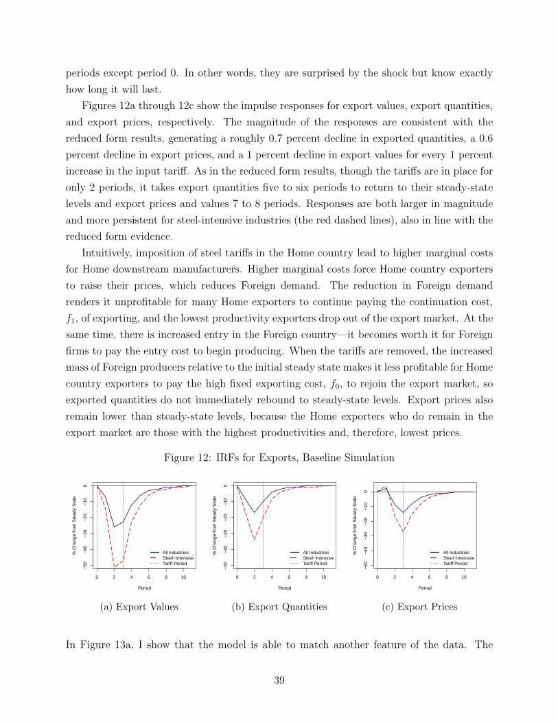
periods except period 0. In other words, they are surprised by the shock but know exactly

how long it will last.

Figures 12a through 12c show the impulse responses for export values, export quantities,

and export prices, respectively. The magnitude of the responses are consistent with the

reduced form results, generating a roughly 0.7 percent decline in exported quantities, a 0.6

percent decline in export prices, and a 1 percent decline in export values for every 1 percent

increase in the input tariff. As in the reduced form results, though the tariffs are in place for

only 2 periods, it takes export quantities five to six periods to return to their steady-state

levels and export prices and values 7 to 8 periods. Responses are both larger in magnitude

and more persistent for steel-intensive industries (the red dashed lines), also in line with the

reduced form evidence.

Intuitively, imposition of steel tariffs in the Home country lead to higher marginal costs

for Home downstream manufacturers. Higher marginal costs force Home country exporters

to raise their prices, which reduces Foreign demand. The reduction in Foreign demand

renders it unprofitable for many Home exporters to continue paying the continuation cost,

f1, of exporting, and the lowest productivity exporters drop out of the export market. At the

same time, there is increased entry in the Foreign country—it becomes worth it for Foreign

firms to pay the entry cost to begin producing. When the tariffs are removed, the increased

mass of Foreign producers relative to the initial steady state makes it less profitable for Home

country exporters to pay the high fixed exporting cost, f0, to rejoin the export market, so

exported quantities do not immediately rebound to steady-state levels. Export prices also

remain lower than steady-state levels, because the Home exporters who do remain in the

export market are those with the highest productivities and, therefore, lowest prices.

Figure 12: IRFs for Exports, Baseline Simulation

0 2 4 6 8 10

−50

−40

−30

−20

−10

0

Period

% C

hang

e fr

om S

tead

y S

tate

All IndustriesSteel−IntensiveTariff Period

(a) Export Values

0 2 4 6 8 10

−50

−40

−30

−20

−10

0

Period

% C

hang

e fr

om S

tead

y S

tate

All IndustriesSteel−IntensiveTariff Period

(b) Export Quantities

0 2 4 6 8 10

−50

−40

−30

−20

−10

0

Period

% C

hang

e fr

om S

tead

y S

tate

All IndustriesSteel−IntensiveTariff Period

(c) Export Prices

In Figure 13a, I show that the model is able to match another feature of the data. The

39

response of domestic production—the dashed light blue line in the figure—to the temporary

shock to steel tariffs is smaller and much less persistent than the response of exports (the

solid, dark blue line). In Figure 13b, I show that the sunk costs of exporting are the key

feature driving persistence in the export response. In this figure, the dashed light blue line

shows the response of exports (quantities) to a simulation of the model in which I remove

the sunk cost of exporting. That is, I set the cost to start exporting, f0, equal to the

continuation cost, f1. Removing the sunk cost completely removes any persistence in the

response of exports to the temporary tariff shock. The baseline response is plotted again in

navy blue for comparison.

Figure 13: Domestic Production and No Sunk Cost

0 2 4 6 8 10

−30

−25

−20

−15

−10

−5

0

Period

% C

hang

e fr

om S

tead

y S

tate

Domestic ProductionExportsTariff Period

(a) Domestic Production

0 2 4 6 8 10

−50

−40

−30

−20

−10

0

Period

% C

hang

e fr

om S

tead

y S

tate

BaselineNo Sunk CostsTariff Period

(b) Export Quantities, No Sunk Cost

7.5.2 Counterfactual Simulation

Next, I simulate a counterfactual in which the steel tariffs are in place for twice as long as in

the baseline simulation—4 periods instead of 2. All other model parameters are unchanged.

The impulse responses for export values, export quantities, and export prices in the counter-

factual are displayed in Figure 14 (the dashed light-blue lines). Tariffs in place for a longer

duration lead to both a larger peak decline in exports and a longer recovery period relative

to the baseline case. In the baseline case, export values took 7 periods after the tariffs were

removed to recover to their initial steady-state levels. In the counterfactual, recovery takes

9 periods.

40

Figure 14: Counterfactual IRFs

0 2 4 6 8 10 12 14

−50

−40

−30

−20

−10

0

Period

% C

hang

e fr

om S

tead

y S

tate

BaselineCounterfactualTariff Period

(a) Export Values

0 2 4 6 8 10 12 14

−50

−40

−30

−20

−10

0

Period

% C

hang

e fr

om S

tead

y S

tate

BaselineCounterfactualTariff Period

(b) Export Quantities

0 2 4 6 8 10 12 14

−50

−40

−30

−20

−10

0

Period

% C

hang

e fr

om S

tead

y S

tate

BaselineCounterfactualTariff Period

(c) Export Prices

7.5.3 Welfare

I use the model to estimate the change in real income, as a result of the temporary tariff

shock in the baseline simulation. In Table 9, I report the annual tariff-induced change in

real income as a percent of GDP and as a percent of exports. In the right-most column,

for comparison, I report the analogous results from the reduced form estimation discussed

in Section 6. While the shape of the model-simulated responses is different from that of the

reduced form estimates, average welfare losses as a percent of exports over 10 periods are

virtually identical between the model and the reduced form estimation at 2.80 percent and

2.79 percent, respectively.

Table 9: Model Estimated Change Welfare

Period % of GDP % of Exports Reduced Form (% of Exports)

0 0 0 01 -0.25 -9.74 -1.37*2 -0.35 -14.98 -3.66*3 -0.08 -3.16 -5.16*4 -0.04 -1.32 -6.36*5 -0.02 -0.68 -4.22*6 -0.01 -0.39 -1.977 -0.01 -0.22 -2.598 0 -0.17 -4.139 0 -0.11 -2.12

10 0 -0.11 0.86Average 0.07 -2.80 -2.79

Next, I calculate the aggregate change in welfare due to the steel tariffs as the sum of the

discounted change in utility relative to steady-state. Table 10 shows the results for the

baseline simulation (two-period tariff) and the counterfactual (four-period tariff). The first

41

row of the table shows the percent change in welfare for each simulation. In the baseline

simulation, the temporary shock leads to welfare losses of 0.08 percent. Losses roughly

double when we double the duration of the tariffs in the counterfactual simulation. To put

these magnitudes into perspective, Alessandria and Choi (2014) show using a similar model

that permanently eliminating an 8 percent tariff on traded goods leads to welfare gains of

just over 1 percent.

The second row of the table shows the share of welfare losses that accrue during the

temporary shock vs the share that accrues after the tariffs are removed. A sizable portion—

20 to 25 percent—of the losses are incurred after the tariffs are lifted. Similar to my reduced

form results, this suggests that ignoring the long-term impacts of temporary tariff shocks

can substantially alter welfare estimates.

Table 10: Model Estimated Change Welfare

Baseline Counterfactual

Pct Change in WF -0.08 -0.15Share Accrued During Shock 81.82 76.31

8 Conclusion

Using a case study of the steel tariffs levied by George W. Bush in 2002-2003 and a newly

devised method for mapping detailed steel inputs to downstream users, I provide the first

comprehensive estimates of the long-term effects that temporary upstream tariffs have on

downstream industries. I find that temporary upstream tariffs have negative impacts on

downstream industries, both in terms of their competitiveness in the export market and

in terms of domestic outcomes like employment and production. Crucially, I find that

these declines are highly persistent, particularly on the export margin and especially for

steel-intensive industries. The global market share of U.S. downstream industries remained

depressed long after the tariffs were removed as foreign buyers permanently shifted sourcing

patterns toward other top producers. Using a dynamic model of trade, I show that the

presence of relationship-specific sunk costs of exporting can generate a persistent response

of downstream exports to a temporary input tariff that is consistent with the patterns I find

in the data. Intuitively, because it is costly for countries to change sources of imports, if an

input tariff induces a change in sourcing patterns, those patterns will not immediately revert

when the tariffs are lifted.

Overall, my results highlight the complex nature of tariff policy in a world with globally

integrated production networks. Even temporary tariffs on a small subset of imports can

42

have persistent effects on a broad swath of the economy. Failing to take this persistence into

account can lead to a substantial underestimate of the welfare implications of tariff policy.

43

References

Alessandria, George and Horag Choi, “Establishment heterogeneity, exporter dynam-

ics, and the effects of trade liberalization,” Journal of International Economics, 2014, 94

(2), 207–223.

Amiti, Mary, Stephen J Redding, and David E Weinstein, “The impact of the 2018

tariffs on prices and welfare,” Journal of Economic Perspectives, 2019, 33 (4), 187–210.

Antras, Pol, Teresa Fort, Agustın Gutierrez, and Felix Tintelnot, “Import Tariffs

and Global Sourcing,” Working Paper, 2021.

Atkeson, Andrew and Ariel Tomas Burstein, “Innovation, firm dynamics, and inter-

national trade,” Journal of political economy, 2010, 118 (3), 433–484.

Bagwell, Kyle and Seung Hoon Lee, “Trade policy under monopolistic competition with

firm selection,” Journal of International Economics, 2020, 127, 103379.

Baldwin, Richard, “Hyteresis in Import Prices: The Beachhead Effect,” American Eco-

nomic Review, 1988, 78 (4), 773–85.

and Paul Krugman, “Persistent trade effects of large exchange rate shocks,” The

Quarterly Journal of Economics, 1989, 104 (4), 635–654.

Bartelsman, Eric J and Wayne Gray, “The NBER manufacturing productivity

database,” Technical Report, National Bureau of Economic Research 1996.

Berlingieri, Giuseppe, Frank Pisch, and Claudia Steinwender, “Organizing global

supply chains: Input cost shares and vertical integration,” Technical Report, National

Bureau of Economic Research 2018.

Blonigen, Bruce A, “Industrial policy and downstream export performance,” The Eco-

nomic Journal, 2016, 126 (595), 1635–1659.

Bown, Chad, Paola Conconi, Aksel Erbahar, and Lorenzo Trimarchi, “Trade pro-

tection along supply chains,” Technical Report, Discussion paper, Mimeo 2020.

Burstein, Ariel and Marc Melitz, “Trade Liberalization and Firm Dynamics,” Advances

in Economics and Econometrics: Volume 2, Applied Economics: Tenth World Congress,

2013, 50, 283.

44

Cavallo, Alberto, Gita Gopinath, Brent Neiman, and Jenny Tang, “Tariff

Passthrough at the Border and at the Store: Evidence from US Trade Policy,” 2019.

Cox, Lydia and Kadee Russ, Will Steel Tariffs Put U.S. Jobs at Risk? 2020. https:

//econofact.org/will-steel-tariffs-put-u-s-jobs-at-risk.

Das, Sanghamitra, Mark J Roberts, and James R Tybout, “Market entry costs,

producer heterogeneity, and export dynamics,” Econometrica, 2007, 75 (3), 837–873.

Demidova, Svetlana and Andres Rodriguez-Clare, “The simple analytics of the Melitz

model in a small economy,” Journal of International Economics, 2013, 90 (2), 266–272.

Dixit, Avinash, “Hysteresis, import penetration, and exchange rate pass-through,” The

Quarterly Journal of Economics, 1989, 104 (2), 205–228.

Eaton, Jonathan and Samuel Kortum, “Technology, geography, and trade,” Economet-

rica, 2002, 70 (5), 1741–1779.

Fajgelbaum, Pablo D, Pinelopi K Goldberg, Patrick J Kennedy, and Amit K

Khandelwal, “The return to protectionism,” The Quarterly Journal of Economics, 2020,

135 (1), 1–55.

Feenstra, Robert C, Philip Luck, Maurice Obstfeld, and Katheryn N Russ, “In

search of the Armington elasticity,” Review of Economics and Statistics, 2018, 100 (1),

135–150.

Flaaen, Aaron and Justin R Pierce, “Disentangling the Effects of the 2018-2019 Tariffs

on a Globally Connected US Manufacturing Sector,” 2019.

Gawande, By Kishore, Pravin Krishna, and Marcelo Olarreaga, “Lobbying compe-

tition over trade policy,” International Economic Review, 2012, 53 (1), 115–132.

Handley, Kyle, Fariha Kamal, and Ryan Monarch, “Rising import tariffs, falling

export growth: When modern supply chains meet old-style protectionism,” Technical

Report, National Bureau of Economic Research 2020.

Irwin, Douglas A, Clashing over commerce: A history of US trade policy, University of

Chicago Press, 2017.

Lake, James and Ding Liu, “Local labor market effects of the 2002 Bush steel tariffs,”

Working Paper 2021.

45

Mayer, Thierry, Marc J Melitz, and Gianmarco IP Ottaviano, “Product mix and

firm productivity responses to trade competition,” The Review of Economics and Statis-

tics, 2016, pp. 1–59.

Melitz, Marc J, “The impact of trade on intra-industry reallocations and aggregate indus-

try productivity,” econometrica, 2003, 71 (6), 1695–1725.

Ossa, Ralph, “A “new trade” theory of GATT/WTO negotiations,” Journal of Political

Economy, 2011, 119 (1), 122–152.

Pierce, Justin R and Peter K Schott, “A concordance between ten-digit US Harmonized

System Codes and SIC/NAICS product classes and industries,” Journal of Economic and

Social Measurement, 2012, 37 (1-2), 61–96.

Romalis, John, “NAFTA’s and CUSFTA’s Impact on International Trade,” The review of

Economics and Statistics, 2007, 89 (3), 416–435.

Schoenle, Raphael, “International menu costs and price dynamics,” Review of interna-

tional economics, 2017, 25 (3), 578–606.

Simonovska, Ina and Michael E Waugh, “The elasticity of trade: Estimates and evi-

dence,” Journal of international Economics, 2014, 92 (1), 34–50.

Venables, Anthony J, “Trade and trade policy with differentiated products: A

Chamberlinian-Ricardian model,” The Economic Journal, 1987, 97 (387), 700–717.

Oscar Jorda, “Estimation and Inference of Impulse Responses by Local Projections,” Amer-

ican Economic Review, March 2005, 95 (1), 161–182.

46

A Appendices

A.1 Steel-Specific IO Table

A.1.1 Data and Merge

I use three data sources to create the steel-specific input output table: exclusion requests

from Regulations.gov, firm-level data from Orbis, and firm-level data from the Dunn &

Bradstreet Database. Data from Regulations.gov are publicly available, and I had access to

the firm-level databases through Harvard’s library.

From Regulations.gov, using their API, I pulled all exclusion requests that were filed

under OMB Form 064-1039 — the form that related to Trump’s Section 232 steel and

aluminum tariffs.

I merge firm names from the exclusion requests with Orbis to match those firms with

NAICS industry classifications. For the merge, I use the fuzzy matching algorithm described

in Appendix 3 of Schoenle (2017). In brief, I standardize all firm names in both databases by

removing capitalization and punctuation, and transforming generic terms (like “Inc.” and

“Co.”) into standard forms. I then merge the databases on firm name and location (U.S.

state). Using this methodology I am able to match about 50 percent of exclusion requesting

firms.

After the merge with Orbis I was left with 12 steel products that were covered by the

Bush tariffs, were covered by the exclusion requests, but that I did not have a merge match

for. I manually searched for exclusion-requesting firms for these products in the Dunn &

Bradstreet database. I was able to match 11 of the 12.

A.1.2 Extending the Steel-Specific IO Methodology to Other Inputs

In this Appendix, I show that the methodology I use to create the steel-specific input-

output table also works for aluminum. In principle, the same methodology should work

for any input that was protected by the Trump tariffs (for which a substantial number of

exclusion requests were filed). In Table 11 shows regressions of changes in material costs in

downstream industries to changes in the unit value of aluminum imports. I link aluminum

imports to industries using the same exclusion-request methodology that I used for the steel

sector. The results show that changes in linked aluminum import unit values are significant

predictors of changes in downstream material costs, even after controlling for the average

price of aluminum.

47

Table 11: Aluminum-Import Prices Predict Downstream Material Costs: Industry-Level

(1) (2)∆ Material Costs ∆ Material Costs

∆ Aluminum Unit Value 0.094 0.153(0.049) (0.049)

∆ PPI Aluminum (Non-Ferrous Metals) 0.530(0.049)

Constant -0.048 -0.009(0.034) (0.033)

Year Fixed Effects Yes No

Sector Fixed Effects Yes YesObservations 650 650

Standard errors in parentheses

Sample years: 2001-2011.

A.1.3 Comparison with Other IO Tables

In Table 12, I list the top 10 downstream using industries of steel according to my steel-

specific IO table, the publicly available IO table from the BEA, and the IO table from

Berlingieri et al. (2018). The differences in these lists highlight the level of detail that my

IO table is able to capture. Instead of representing industry use of all steel products, my IO

table represents industry use of a very specific set of steel products—those that were covered

by the Bush steel tariffs.

A.2 Raw Regression Results

Due to the inherently noisy quality of export price (unit value) and quantity data available

from Customs, in the main body of the paper I smooth price and quantity regressions over a

rolling two-year window. The raw results are presented here for transparency—the impulse

responses take the same shape as the smoothed results, but are estimated with less precision.

48

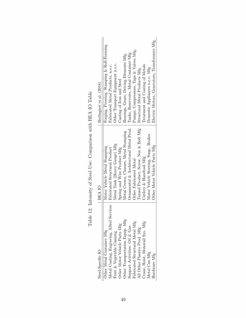
Tab

le12

:In

tensi

tyof

Ste

elU

se:

Com

par

ison

wit

hB

EA

IOT

able

Ste

el-S

pec

ific

IOB

EA

IOB

erli

ngie

riet

al.

(2018)

Oth

erM

etal

Con

tain

erM

fgM

oto

rV

ehic

leM

etal

Sta

mp

ing

Forg

ing,

Pre

ssin

g,

Sta

mp

ing

&R

oll

-Form

ing

Met

alC

oati

ng,

Engr

avin

g,A

llie

dS

ervic

esF

ab

rica

ted

Str

uct

ura

lP

rod

uct

Fab

rica

ted

Met

al

Pro

du

cts,

n.e

.c.

Fru

it&

Veg

etab

leC

ann

ing

Met

al

Tan

k(H

eavy

Gau

ge)

Mfg

Oth

erT

ran

sport

Equ

ipm

ent

n.e

.c.

Oth

erM

otor

Veh

icle

Par

tsM

fgS

pri

ng

an

dW

ire

Pro

du

ctM

fgC

ast

ing

of

Iron

an

dS

teel

Oth

erT

ran

spor

tati

onE

qu

ip.

Mfg

Met

al

Cro

wn

,C

losu

re,

Met

al

Sta

mp

ing

Bea

rin

gs,

Gea

rs,

Dri

vin

gE

lem

ents

Mfg

.S

up

por

tA

ctiv

itie

s:O

il&

Gas

Orn

am

enta

l&

Arc

hit

ectu

ral

Met

al

Pro

d.

Tan

ks,

Res

ervo

irs,

Met

al

Conta

iner

Mfg

.F

abri

cate

dS

tru

ctu

ral

Met

alM

fgO

ther

Fab

rica

ted

Met

al

Pu

mp

s,C

om

pre

ssors

,T

ap

s&

Valv

esM

fg.

All

Oth

erP

last

ics

Pro

d.

Mfg

Tu

rned

Pro

du

ct,

Scr

ew,

Nu

t&

Bolt

Mfg

Str

uct

ura

lM

etal

Pro

du

cts

Mfg

.C

ran

e,H

oist

,M

onor

ail

Sys.

Mfg

Cu

tler

y&

Han

dto

ol

Mfg

Tre

atm

ent

an

dC

oati

ng

of

Met

als

Met

alC

anM

fgM

oto

rV

ehic

leS

teer

ing,

Su

sp.,

Bra

kes

Dom

esti

cA

pp

lian

ces

n.e

.c.

Mfg

Har

dw

are

Mfg

Oth

erM

oto

rV

ehic

leP

art

sM

fgE

lect

ric

Moto

rs,

Gen

erato

rs,

Tra

nsf

orm

ers

Mfg

.

49

Figure 15: Effect of Higher Statutory Rates on Downstream Exports

−4

−2

02

4

Year(tick at start of period)

Res

pons

e to

1 p

.p. I

ncre

ase

in S

tatu

tory

Rat

e

ResponseTariff Period 90% CI

All DownstreamAbove Median Intensity

1997 2001 2005 2009 2013

(a) Export Quantities−

4−

20

24

Year(tick at start of period)

Res

pons

e to

1 p

.p. I

ncre

ase

in S

tatu

tory

Rat

e

ResponseTariff Period 90% CI

All DownstreamAbove Median Intensity

1997 2001 2005 2009 2013

(b) Export Prices

A.3 Underlying Dynamics

A.3.1 Shifting to Exempt Countries

While results presented above show that upstream tariffs have negative consequences for

downstream industries, the impacts are not always direct. Safeguard remedies like the steel

tariffs are put in place to reduce import competition. In theory, if buyers face a higher foreign

price, they will be more likely to buy from a domestic producer. In practice, however, the

choice is more complicated. The buyer of a previously imported product has two choices

when faced with a new import tariff: (1) continue buying the imported product and pay the

added cost of the tariff, or (2) switch suppliers and purchase from a country that is exempt

from the tariff (note, this would include purchasing from a domestic source). Trade data can

shed light on the choices that domestic buyers made when the Bush tariffs were enacted. The

left panel of Figure 16 shows that there was not a meaningful difference in the quantity of

protected steel products imported into the United States during the 2002-2003 period. What

does change, however, during the tariff period is the source of those imports. The right panel

of Figure 16 shows that there is a sharp increase in the share of protected imports coming

from countries that were exempt from the tariffs. This change in the sourcing pattern of

protected steel products lasts until the tariffs are lifted; soon after, import shares return to

roughly pre-tariff levels.

To test whether industries that use inputs for which a larger share were shifted to exempt

50

Figure 16: Imports of Protected Steel Products

1996 1998 2000 2002 2004 2006 2008

0.5

1.0

1.5

2.0

2.5

3.0

Year

Mill

ion

Met

ric T

ons

(a) Total Imports, All Countries

1996 1998 2000 2002 2004 2006 2008

0.0

0.2

0.4

0.6

0.8

1.0

Year

Sha

re o

f Tot

al Im

port

s

ExemptNon−Exempt

(b) Exempt vs. Non-Exempt Share

countries fared better than industries that did not shift sources, I run the same regression

from equation 2, but also include the change in share of inputs coming from exempt countries

between 2001 and 2003—∆exempt share— on the right hand side. I plot the response of

the change in the U.S. export share since 2001 to changes in ∆exempt share in Figure 17.

The results show that industries that use inputs for which a larger share was shifted to come

from exempt countries suffered a smaller relative decline in global market share.

To assuage potential concerns that the ability to shift sources is systematically related to

long-term industry performance, I compare industry performance prior to the tariffs in terms

of growth (or decline) in global market share to the change in exempt source share once the

tariffs are in place. Specifically, the correlation between the change in an industry’s export

share between 1995 and 2000 (pre-tariff) and the amount that the industry shifts sources

to exempt countries is 0.031 with a standard error of 0.033. In other words, industries for

which inputs shifted sources in response to the tariffs were doing no better in terms of export

shares prior to the tariff. (This lack of pre-trend can also be seen for 2001-2002 in Figure 17.)

There are two factors that do appear to drive the shift toward exempt sources for up-

stream products in response to the tariffs: the level of the tariff, and the share of the product

that was being sourced from exempt countries in 2001, prior to the tariffs. The first column

in Table 13 shows that upstream products that faced a higher statutory tariff rate were

more likely to shift toward an exempt source—intuitively, if we assume there is a fixed cost

to shifting sources, a higher tariff makes it more likely that the benefit of shifting would

outweigh the cost. The second column divides upstream products into four groups: those

51

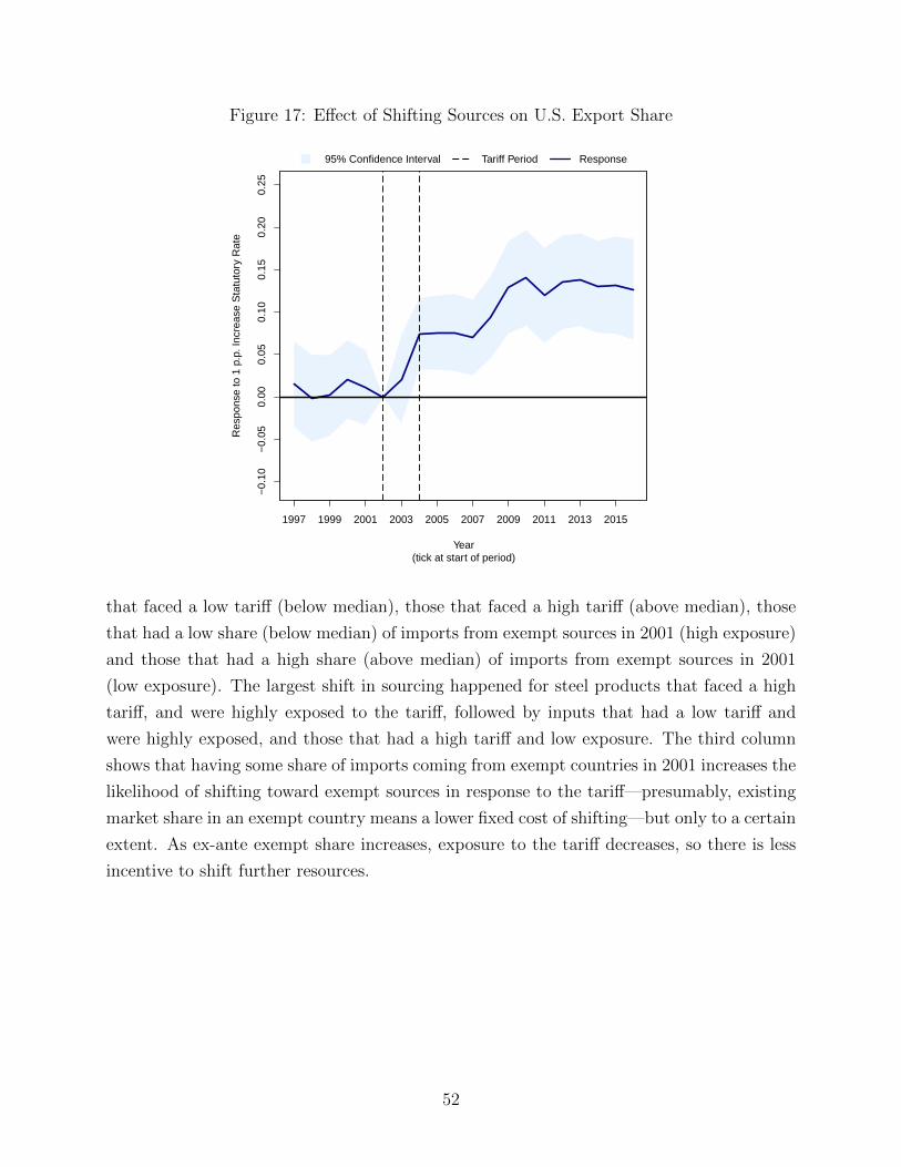
Figure 17: Effect of Shifting Sources on U.S. Export Share

−0.

10−

0.05

0.00

0.05

0.10

0.15

0.20

0.25

Year(tick at start of period)

Res

pons

e to

1 p

.p. I

ncre

ase

Sta

tuto

ry R

ate

Response95% Confidence Interval Tariff Period

1997 1999 2001 2003 2005 2007 2009 2011 2013 2015

that faced a low tariff (below median), those that faced a high tariff (above median), those

that had a low share (below median) of imports from exempt sources in 2001 (high exposure)

and those that had a high share (above median) of imports from exempt sources in 2001

(low exposure). The largest shift in sourcing happened for steel products that faced a high

tariff, and were highly exposed to the tariff, followed by inputs that had a low tariff and

were highly exposed, and those that had a high tariff and low exposure. The third column

shows that having some share of imports coming from exempt countries in 2001 increases the

likelihood of shifting toward exempt sources in response to the tariff—presumably, existing

market share in an exempt country means a lower fixed cost of shifting—but only to a certain

extent. As ex-ante exempt share increases, exposure to the tariff decreases, so there is less

incentive to shift further resources.

52

Table 13: Drivers of Shift to Exempt Sources

(1) (2) (3)∆ Exempt Share ∆ Exempt Share ∆ Exempt Share

Tariff Rate 0.569 0.603(0.262) (0.240)

Low Tariff × Low Exposure 0.000(.)

Low Tariff × High Exposure 0.174(0.071)

High Tariff × Low Exposure 0.136(0.059)

High Tariff × High Exposure 0.228(0.059)

Exempt Share 2001 0.658(0.203)

Squared Exempt Share 2001 -0.951(0.214)

Observations 169 169 169

Standard errors in parentheses

A.4 Global Reconfiguration: China

Figure 18 shows that, unlike Germany, Japan and France (shown in the main body of the

paper), U.S. export shares do not appear to have shifted persistently toward China in the

wake of the steel tariffs.

53

Figure 18: Chinese Export Shares

−0.

20.

00.

20.

4

Year(tick at start of period)

Res

pons

e to

1 p

.p. I

ncre

ase

in S

tatu

tory

Rat

e

ResponseTariff Period 90% CI

All DownstreamAbove Median Intensity

1997 2001 2005 2009 2013

A.5 Model

In this appendix I provide further detail on the model presented in Section 7, its equilibrium

conditions, and the solution method.

A.5.1 Equations for the Model Solution

Steel Production occurs both at home (s) and abroad (ω) using the production technolo-

gies:

st = A`t (9)

ωt = A∗`∗t , (10)

where A is a country-specific productivity parameter. Steel is tradable, and downstream

goods in each country are produced using a CES composite of home and foreign steel inputs.

54

St =[sε−1ε

t + ωε−1ε

t

] εε−1

, (11)

where ε is the elasticity of substitution between home and foreign steel. Steel consumption

in the foreign country is analogous (unless otherwise noted, assume this is teh case going

forward). Foreign variables will be demarcated with an asterisk going forward. Prices of

home and foreign steel are given by ps,t and pω,t, respectively. The home government can

place a tariff, τs on imported steel, so that the price of foreign steel in the home country is

given by (1 + τs)pω,t. The price of the composite steel product is standard:

P St =

[(ps,t)

1−ε + ((1 + τs)pω,t)1−ε] 1

1−ε (12)

Demand for home and foreign steel in the home country will be given, respectively, by:

sdt =

(ps,tP St

)−εSt and ωdt =

((1 + τs)pω,t

P St

)−εSt (13)

Outside Good Sector. The outside consumption good, DO, is produced (linearly) with

labor and is sold in a competitive market. DO is produced in both countries and is freely

traded, thus I treat the outside good as the numeraire and normalize wages in both countries,

W and W ∗ to 1.

Households choose consumption and investment to maximize utility:

VC,0 = max∞∑t=0

βtU(Ct) (14)

subject to the sequence of budget constraints:

PtCt +QtBt ≤ PtWtLt +Bt−1 + PtΠt + PtTt (15)

Where β ∈ (0, 1) is the time discount factor, Ct is consumption of final goods, Qt and Bt

are the price of and quantity of bond holdings, Wt is the real wage rate, Πt are profits from

domestic producers, and Tt is a real lump-sum transfer from the home government to the

55

households that includes tariff revenue collected in the steel sector. Households have log

utility over consumption of the final good, whose composition is described next.

Final Good Producers.

There is a final good production sector that assembles the consumption good—a Cobb-

Douglas composite of the outside good, DO and the manufactured good, DT :

Dt = DγT,tD

1−γO,t (16)

where DT,t is a CES composite of domestic and foreign tradeable manufactured goods,

yH,t(z, v, x) and yF,t(z, v, x):

DT =

[1∑

m=0

∫∫yH,t(z, v, x)

ρ−1ρ ψT,t(z, v, x)dz + yF,t(z, v, x)

ρ−1ρ ψ∗T,t(z, v, 1)dzdv

] ρρ−1

(17)

Here, (z, v, x) is a technology triplet that defines downstream firms and will be defined in

the next section, ψT (z, v, x) and ψ∗T (z, v, 1) are the distributions of downstream producers in

the Home country and downstream exporters in the Foreign country, and θ is the elasticity

of substitution among downstream manufactured goods.

Demand for each of the downstream goods will be given by:

ydH,t =

(pH,tPT,t

)−θDT = p−θH,tP

θ−1T PtDt (18)

ydF,t =

(PF,tPT,t

)−θDT = p−θF,tP

θ−1T PtDt (19)

Where PT,t is the price index of the downstream manufactured composite good, DT is total

demand for the composite good, and Pt is the price index of the aggregate consumption

good, Dt.

Downstream Manufacturing Sector

Downstream good producers are heterogeneous with respect productivity, and therefore, ex-

port status. The set-up of the downstream sector is adapted from Alessandria and Choi

(2014). Incumbent firms have idiosyncratic productivity, z, which follows a first-order

Markov process where a firm’s probability of having productivity z′ in period t+ 1 given it

has productivity z in period t is given by Φ(z′|z). Next-period productivity, z′ is bounded

56

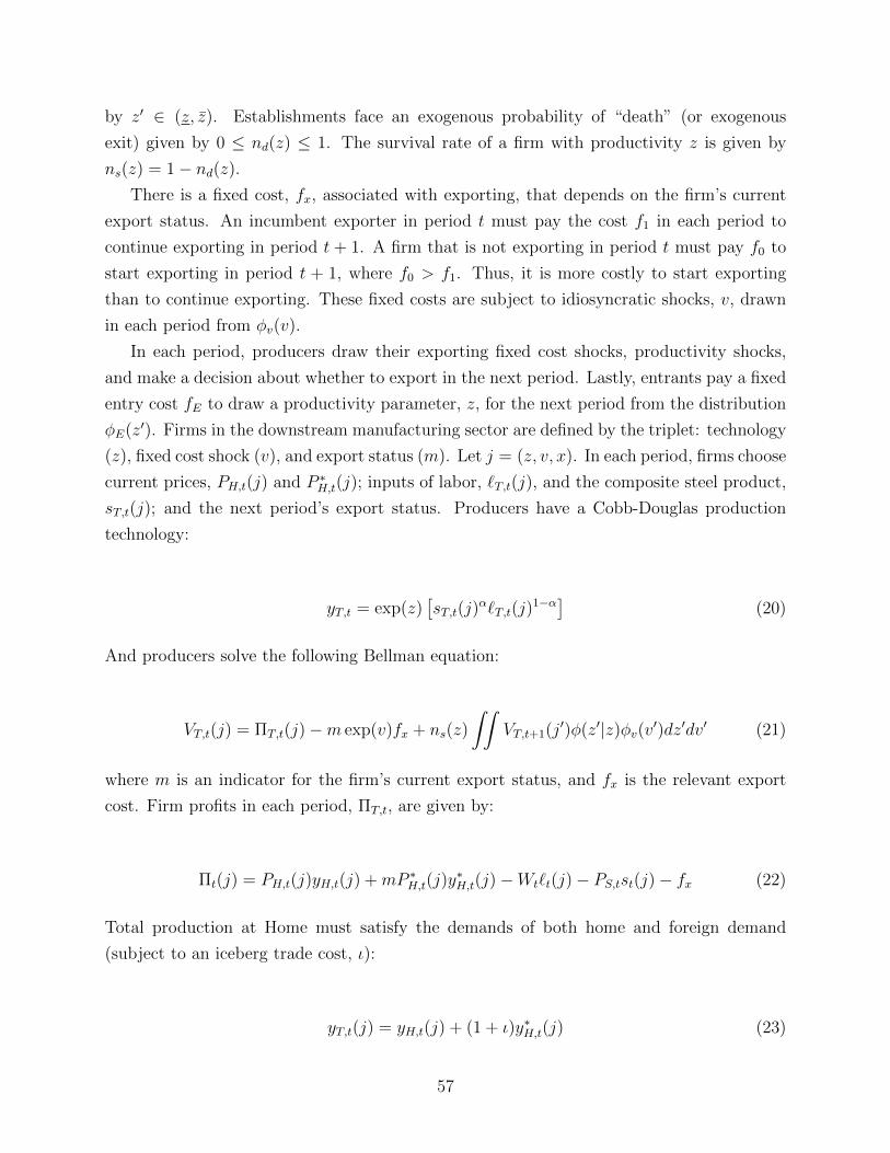
by z′ ∈ (z, z). Establishments face an exogenous probability of “death” (or exogenous

exit) given by 0 ≤ nd(z) ≤ 1. The survival rate of a firm with productivity z is given by

ns(z) = 1− nd(z).

There is a fixed cost, fx, associated with exporting, that depends on the firm’s current

export status. An incumbent exporter in period t must pay the cost f1 in each period to

continue exporting in period t + 1. A firm that is not exporting in period t must pay f0 to

start exporting in period t + 1, where f0 > f1. Thus, it is more costly to start exporting

than to continue exporting. These fixed costs are subject to idiosyncratic shocks, v, drawn

in each period from φv(v).

In each period, producers draw their exporting fixed cost shocks, productivity shocks,

and make a decision about whether to export in the next period. Lastly, entrants pay a fixed

entry cost fE to draw a productivity parameter, z, for the next period from the distribution

φE(z′). Firms in the downstream manufacturing sector are defined by the triplet: technology

(z), fixed cost shock (v), and export status (m). Let j = (z, v, x). In each period, firms choose

current prices, PH,t(j) and P ∗H,t(j); inputs of labor, `T,t(j), and the composite steel product,

sT,t(j); and the next period’s export status. Producers have a Cobb-Douglas production

technology:

yT,t = exp(z)[sT,t(j)

α`T,t(j)1−α] (20)

And producers solve the following Bellman equation:

VT,t(j) = ΠT,t(j)−m exp(v)fx + ns(z)

∫∫VT,t+1(j′)φ(z′|z)φv(v

′)dz′dv′ (21)

where m is an indicator for the firm’s current export status, and fx is the relevant export

cost. Firm profits in each period, ΠT,t, are given by:

Πt(j) = PH,t(j)yH,t(j) +mP ∗H,t(j)y∗H,t(j)−Wt`t(j)− PS,tst(j)− fx (22)

Total production at Home must satisfy the demands of both home and foreign demand

(subject to an iceberg trade cost, ι):

yT,t(j) = yH,t(j) + (1 + ι)y∗H,t(j) (23)

57

Profit-maximization will lead to optimal production of:

yH,t =1

2γ[α− ηQ−MCT,t exp(−z)]

y∗H,t =1

2γ

[α− ηQ∗ −MCT,t exp(−z)(1 + ι)−1

](24)

Where Q =∫

Ωy(z)dz and Ω is the set of available varieties.

where MCT,t is the marginal cost of production for a tradeable good producer with z = 0.

MCT,t =

[(PStα

)α(Wt

1− α

)1−α]

(25)

and DT,t is total demand for the composite tradeable good and PT,t is the price index of the

composite tradeable good at time t:

PT =

(1∑

m=0

∫z×v

PH,t(z, v, x)1−θψT,t(z, v, x)dzdv +

∫z×v

PF,t(z, v, 1)1−θψ∗T,t(z, v, 1)dzdv

) 11−θ

(26)

ψT,t(z, v, x), above, is the distribution of downstream producers in the home country and

ψ∗T,t is the distribution of exporters in the foreign country. Total production for a firm will

be given by:

yT,t =

[θ

θ − 1MCT,t

]−θexp(θz)

(P θT,tDT,t + (1 + ι)1−θP ∗θT,tD

∗T,t

)(27)

Let the value of a producer j that decides to export in period t+ 1 be:

V 1T,t(j) = max ΠT,t(j)− exp(v)fx + nsQt

∫∫VT,t+1(z′, v′, 1)φ(z′|z)φv(v

′)dz′dv′ (28)

And let the value of a producer j that does not export in period t+ t be:

V 0T,t(j) = max ΠT,t(j) + nsQt

∫∫VT,t+1(z′, v′, 0)φ(z′|z)φv(v

′)dz′dv′ (29)

58

Then, the actual value of a producer will be equal to VT,t(j) = maxV 1T,t, V

0T,t. As is

standard, there will exist a productivity threshold, zm,t(v) such that an establishment is

indifferent between exporting and not exporting. This export threshold will depend on the

establishment’s current export status, m, productivity, z, and fixed cost shock v.

Lastly, new establishments are created by incurring a fixed entry cost, fE, in the period

prior to production. Entrants draw a productivity z from the distribution φE(z′) and entrants

cannot export in their first period of production. Free entry requires that:

V ET,t = fE +Qt

∫∫VT,t+1(z′, v′, 0)φE(z′)φ(v′)dz′dv′ ≤ 0 (30)

Aggregation. Integrating over producers, aggregate production in the home country down-

stream industries will be given by:

HT,t =

[θ

θ − 1MCT,t

]−θP θT,tDT,t

[ΨT,t + u(1 + ι)1−θΨX,t

](31)

where u = P ∗θT,tD∗T,t/P

θT,tDT,t and

ΨT,t =

∫∫exp((θ − 1)z)ψT,t(z, v, x)dzdv (32)

ΨX,t =

∫∫exp((θ − 1)z)ψX,t(z, v, 1)dzdv (33)

Aggregate steel and labor used for production will be given by:

ST,t = α

(MCT,tP St

)HT,t (34)

LT,t =1− αα

P St ST,t (35)

A.5.2 Equilibrium

In an equilibrium, variables satisfy a number of resource constraints. The final goods market

clearing conditions are met in both countries:

Dt = Ct

59

The steel market clears in both countries:

st + ωt = sdt + ωdt

And:

St = ST,t

Labor market clearing condition are met:

L = LS + LO + LT + LF

Where LF = fE ∗ NE + f0

∫∫ zz0,t(v)

exp(v)ψT,t(z, v, 0)dzdv + f1

∫∫ zz1,t(v)

exp(v)ψT,t(z, v, 1)dzdv

is labor used to cover the fixed costs of entry and exporting. Feasibility conditions are met

in the market for downstream manufactured goods in both countries:

YH,t = yH,t + (1 + ι)y∗H,t

And tariff revenue and profits are distributed to households. An equilibrium is a collection

of consumption allocations for home and foreign consumers, C, Bt, C∗t and B∗t ; allocations,

prices, and export decisions for home and foreign manufacturing producers; prices and allo-

cations for outside sector producers; labor used for exporting and entry costs at home and

in foreign, and transfers by home and foreign governments, bond prices, Qt. The allocations

are such that:

• Households maximize utility (14)

• Final good producers maximize profits. (25)

• Downstream producers choose steel inputs, labor inputs, and prices to maximize profits.

(18)

• Free entry conditions are met in the downstream sector. (30)

• Market clearing conditions hold.

A.5.3 Calibration

Here I will describe the calibration. When available, I start with the parameters set at the

levels used by Alessandria and Choi (2014) which are set to target empirical moments de-

scribing the distribution of U.S. manufacturing establishments in 1987. I make adjustments

60

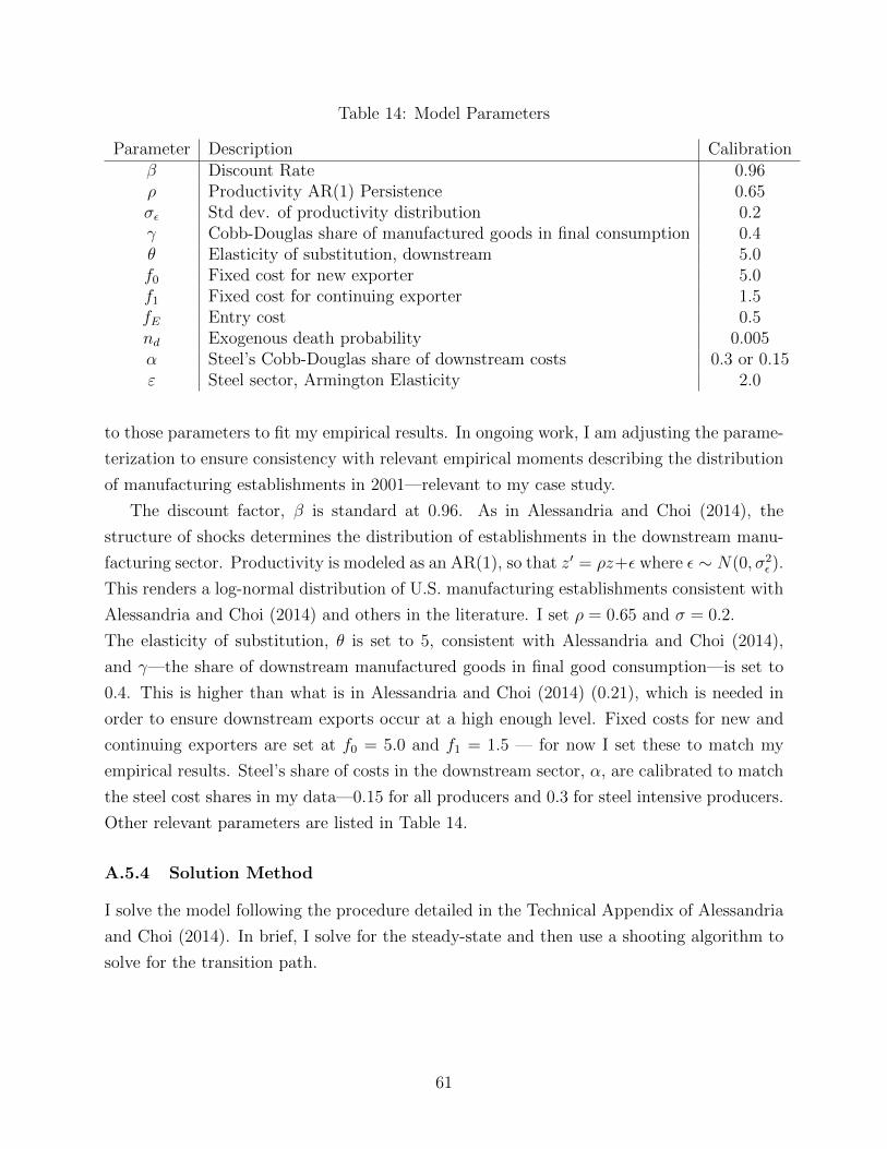
Table 14: Model Parameters

Parameter Description Calibrationβ Discount Rate 0.96ρ Productivity AR(1) Persistence 0.65σε Std dev. of productivity distribution 0.2γ Cobb-Douglas share of manufactured goods in final consumption 0.4θ Elasticity of substitution, downstream 5.0f0 Fixed cost for new exporter 5.0f1 Fixed cost for continuing exporter 1.5fE Entry cost 0.5nd Exogenous death probability 0.005α Steel’s Cobb-Douglas share of downstream costs 0.3 or 0.15ε Steel sector, Armington Elasticity 2.0

to those parameters to fit my empirical results. In ongoing work, I am adjusting the parame-

terization to ensure consistency with relevant empirical moments describing the distribution

of manufacturing establishments in 2001—relevant to my case study.

The discount factor, β is standard at 0.96. As in Alessandria and Choi (2014), the

structure of shocks determines the distribution of establishments in the downstream manu-

facturing sector. Productivity is modeled as an AR(1), so that z′ = ρz+ε where ε ∼ N(0, σ2ε ).

This renders a log-normal distribution of U.S. manufacturing establishments consistent with

Alessandria and Choi (2014) and others in the literature. I set ρ = 0.65 and σ = 0.2.

The elasticity of substitution, θ is set to 5, consistent with Alessandria and Choi (2014),

and γ—the share of downstream manufactured goods in final good consumption—is set to

0.4. This is higher than what is in Alessandria and Choi (2014) (0.21), which is needed in

order to ensure downstream exports occur at a high enough level. Fixed costs for new and

continuing exporters are set at f0 = 5.0 and f1 = 1.5 — for now I set these to match my

empirical results. Steel’s share of costs in the downstream sector, α, are calibrated to match

the steel cost shares in my data—0.15 for all producers and 0.3 for steel intensive producers.

Other relevant parameters are listed in Table 14.

A.5.4 Solution Method

I solve the model following the procedure detailed in the Technical Appendix of Alessandria

and Choi (2014). In brief, I solve for the steady-state and then use a shooting algorithm to

solve for the transition path.

61

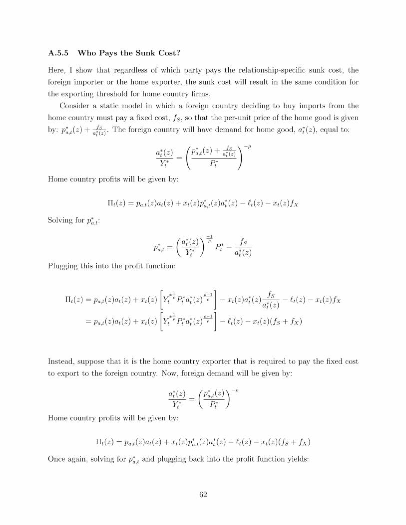
A.5.5 Who Pays the Sunk Cost?

Here, I show that regardless of which party pays the relationship-specific sunk cost, the

foreign importer or the home exporter, the sunk cost will result in the same condition for

the exporting threshold for home country firms.

Consider a static model in which a foreign country deciding to buy imports from the

home country must pay a fixed cost, fS, so that the per-unit price of the home good is given

by: p∗a,t(z) + fSa∗t (z)

. The foreign country will have demand for home good, a∗t (z), equal to:

a∗t (z)

Y ∗t=

(p∗a,t(z) + fS

a∗t (z)

P ∗t

)−ρHome country profits will be given by:

Πt(z) = pa,t(z)at(z) + xt(z)p∗a,t(z)a∗t (z)− `t(z)− xt(z)fX

Solving for p∗a,t:

p∗a,t =

(a∗t (z)

Y ∗t

)−1ρ

P ∗t −fSa∗t (z)

Plugging this into the profit function:

Πt(z) = pa,t(z)at(z) + xt(z)

[Y∗ 1ρ

t P ∗t a∗t (z)

ρ−1ρ

]− xt(z)a∗t (z)

fSa∗t (z)

− `t(z)− xt(z)fX

= pa,t(z)at(z) + xt(z)

[Y∗ 1ρ

t P ∗t a∗t (z)

ρ−1ρ

]− `t(z)− xt(z)(fS + fX)

Instead, suppose that it is the home country exporter that is required to pay the fixed cost

to export to the foreign country. Now, foreign demand will be given by:

a∗t (z)

Y ∗t=

(p∗a,t(z)

P ∗t

)−ρHome country profits will be given by:

Πt(z) = pa,t(z)at(z) + xt(z)p∗a,t(z)a∗t (z)− `t(z)− xt(z)(fS + fX)

Once again, solving for p∗a,t and plugging back into the profit function yields:

62

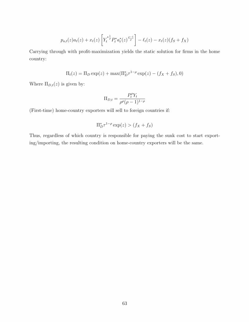
pa,t(z)at(z) + xt(z)

[Y∗ 1ρ

t P ∗t a∗t (z)

ρ−1ρ

]− `t(z)− xt(z)(fS + fX)

Carrying through with profit-maximization yields the static solution for firms in the home

country:

Πt(z) = ΠD exp(z) + max(Π∗Dτ1−ρ exp(z)− (fX + fS), 0)

Where ΠD,t(z) is given by:

ΠD,t =P ρt Yt

ρρ(ρ− 1)1−ρ

(First-time) home-country exporters will sell to foreign countries if:

Π∗Dτ1−ρ exp(z) > (fX + fS)

Thus, regardless of which country is responsible for paying the sunk cost to start export-

ing/importing, the resulting condition on home-country exporters will be the same.

63