the long run effects of changes in tax...

Contents lists available at ScienceDirect

Journal of Economic Dynamics & Control

Journal of Economic Dynamics & Control 35 (2011) 1451–1473

0165-18

doi:10.1

� Cor

E-m1 M2 El

journal homepage: www.elsevier.com/locate/jedc

The long run effects of changes in tax progressivity

Daniel R. Carroll a,�, Eric R. Young b

a Research Department, Federal Reserve Bank of Cleveland, United Statesb Department of Economics, University of Virginia, United States

a r t i c l e i n f o

Article history:

Received 15 July 2010

Accepted 18 February 2011Available online 3 July 2011

JEL classification:

E21

E25

E62

Keywords:

Heterogeneity

Progressive taxation

Inequality

89/$ - see front matter & 2011 Elsevier B.V. A

016/j.jedc.2011.06.004

responding author.

ail addresses: [email protected] (D.R. Carro

eh (2005) considers how progressive taxatio

astic labor supply and/or borrowing constrai

a b s t r a c t

This paper compares the steady-state outcomes of revenue-neutral changes to the

progressivity of the tax schedule. Our economy features heterogeneous households who

differ in their preferences and permanent labor productivities, but it does not have

idiosyncratic risk. We find that increases in the progressivity of the tax schedule are

associated with long-run distributions with greater aggregate income, wealth, and labor

input. Average hours generally declines as the tax schedule becomes more progressive

implying that the economy substitutes away from less-productive workers toward

more-productive workers. Finally, as progressivity increases, income inequality is

reduced and wealth inequality rises. Many of these results are qualitatively different

than those found in models with idiosyncratic risk, and therefore suggest closer

attention should be paid to modeling the insurance opportunities of households.

& 2011 Elsevier B.V. All rights reserved.

1. Introduction

The purpose of this paper is to study the effects of flattening progressive tax functions when there is no risk. Theliterature on the gains from flattening the tax code is large — some recent quantitative examples include Ventura (1999),Castaneda et al. (1998), Dıaz-Gimenez and Pijoan-Mas (2006), Conesa and Krueger (2006), and Conesa et al. (2009). All ofthese papers begin with the presumption that insurance markets are absent (as in Aiyagari, 1994); progressive taxationtherefore has beneficial insurance properties, as it reduces the variance of labor income.1 It turns out that a robustprediction of these models is that aggregate activity and welfare respond positively to ‘‘flattening’’ the tax code. Table 1illustrates how assumptions about the nature of income and wealth inequality lead to different predictions about theeffects of flattening the tax code. In contrast, we approach the problem from the other end of the spectrum — we ask howprogressive tax reform would effect the economy in a model without any uncertainty where inequality is entirely due toimmutable heterogeneity in preferences and endowments.

Constructing a model that matches the US distributions of income and wealth not based on idiosyncratic risk is difficultgiven the results we found in Carroll and Young (2009). In the absence of discount factor heterogeneity, deterministicmodels with progressive taxation predict that the stationary distribution will have a negative correlation between incomeand wealth and between capital and labor income, both of which are inconsistent with US data.2 To get around theseproblems, we construct distributions of discount factors, labor productivities, and labor supply disutilities that exactly

ll rights reserved.

ll), [email protected] (E.R. Young).

n affects the economy in a world with risky saving via entrepreneurial activity.

nts do not affect those results.

www.elsevier.com/locate/jedc

dx.doi.org/10.1016/j.jedc.2011.06.004

mailto:[email protected]

mailto:[email protected]

dx.doi.org/10.1016/j.jedc.2011.06.004

dx.doi.org/10.1016/j.jedc.2011.06.004

Table 1

Flat tax experiments Setup Types of risk Effect on aggregates Effect on distribution

Conesa and Krueger (2006) OLG Idiosyncratic wages, death Y, K, H, N, C, r increase Giniy ,Ginik increase

Ventura (1999) OLG Idiosyncratic wages, death Y, K, N increase, H unchanged,

r decreaseGiniy ,Ginik increase

Dıaz-Gimenez and

Pijoan-Mas (2006)

OLG/dynastic Idiosyncratic wages, retirement, death Y, K, H, N, C, r increase Giniy ,Ginik ,Ginic increase

Castaneda et al. (1998) OLG/dynastic Idiosyncratic wages, retirement, death Y, K, H, N, C, r increase Giniy ,Ginik ,Ginic increase

D.R. Carroll, E.R. Young / Journal of Economic Dynamics & Control 35 (2011) 1451–14731452

match the distributions of assets, income, and labor hours in the model to those in the data. We use this model toinvestigate the response of the economy to changes in the progressivity of the income tax code.3

The qualitative and quantitative implications of tax reforms in our model are quite different than those in theincomplete market literature. We conduct three revenue-neutral tax reform experiments and find that flattening the taxcode – reducing the progressivity of the income tax – tends to reduce aggregate capital and labor input, rather thanincrease it; the decrease is also quantitatively large. More progressive marginal tax schedules can lead to steady stateswith as much as 47% more aggregate capital and 40% more labor input. The results of our other experiments, though lesspronounced, consistently find that tax reforms with more progressive schedules increase aggregate capital and labor input.We also find that more progressivity generally decreases income inequality but increases wealth inequality. These changesoccur without any change in the average tax rate in the economy, since we impose revenue neutrality on our experiments.With respect to labor input, progressivity increases labor input because it reallocates labor from less productive to more-productive agents, generating output gains even though labor supply – measured by raw hours – actually declines. Thedriving factor behind both of these findings comes from the heterogeneous response of households to changes in marginalincome tax rates. Households with identical discount factors have the same level of long-run income, and thus face thesame marginal income tax rate; however, these same households may differ with respect to their labor productivity anddisutility of labor. When this occurs, these households will face different marginal utility costs from adjusting saving andlabor. As a result, they will not choose the same composition of income between labor income and capital income.

Our results have two implications. First, endogenizing the extent to which the private sector can provide insurance – asin Krueger and Perri (2011) or Abraham and Carceles-Poveda (2009) – may be critical for understanding whetherprogressive taxation increases or decreases aggregate activity. In our model, the government does not crowd out insurancemarkets because they are already complete, while in the incomplete market literature the government also does not crowdout insurance because there are no such markets. If the government cannot provide insurance without crowding outexisting sources, then the welfare gains from adjusting the tax code may be significantly smaller than those found in theliterature to date.

Second, the extent to which inequality is driven by preferences vs. endowments also will play a role in determining theeffects of progressive taxation, as they do in determining the effects of eliminating the business cycle (see Krusell et al.,2009).4 Castaneda et al. (2003) show that a model with only labor efficiency shocks (and stochastic mortality) can matchthe main facts about US wealth, earnings, and consumption inequality, without any preference heterogeneity. To makethe model fit the data, they argue that direct estimates of the wage process are unreliable, since they do not include thewealthiest households (who also contribute disproportionately to earnings). They do not attempt to match the incomeprocess for those individuals who can be observed, however, and also do not include any preference heterogeneity. It is anopen question what part preference heterogeneity plays in US inequality, and our results suggest that it is potentiallyimportant for policy questions.5 It is also an open question how to calibrate a model in a way that separately identifiespreference heterogeneity and shocks, but again based on our results it appears that such a model may be needed tomeasure the effects of progressivity.

2. Model

The model economy is composed of three sectors: a stand-in firm, a government, and a unit measure of heterogeneoushouseholds.

2.1. Households

The economy is populated by a finite set I of households of unit measure. These households differ ex ante along threedimensions: their discount factor b, their permanent labor productivity e, and their disutility from labor B. Every

3 Saez (2002) uses a similar model in which the only heterogeneity is in initial wealth.4 Davila et al. (2005) and Athreya et al. (2009) show that optimal taxation in a model of uninsurable idiosyncratic risk has a progressive aspect to it.

The extent of this progressivity seems likely to be related to the preferences vs. endowments issue as well.5 Badel and Huggett (2010) show that preference shocks in an OLG setting can replicate some key facts of inequality in the US.

D.R. Carroll, E.R. Young / Journal of Economic Dynamics & Control 35 (2011) 1451–1473 1453

household is endowed with 1 unit of discretionary time which it may allocate to leisure, ‘, or labor, h. Any household i 2 I

has preferences over consumption, c, and leisure which are described by the following lifetime utility function:

Ui ¼X1t ¼ 0

bti logðcitÞþBi

‘1�sit

1�s

" #, Bi40: ð2:1Þ

sZ0 is the inverse of the Frisch elasticity of leisure and is assumed uniform across households.6 While we do not focus onsustained growth, the utility function is consistent with a balanced-growth path along which leisure and labor supply areconstant.

2.2. Firm

Each period, a stand-in firm uses capital and labor input to produce output according to a production technology F(K,N).Let F(K,N) be strictly concave and increasing in K and N and F(0,N)¼F(K,0)¼0. Output may be consumed or investedtoward future capital. The firm rents inputs from the households through perfectly competitive markets. Letting theproduction technology be Cobb–Douglas with capital share parameter a 2 ½0,1�, profit-maximization implies that eachinput is paid its marginal product:

rt ¼ F1ðK ,NÞ ¼ aKa�1N1�a,

wt ¼ F2ðK ,NÞ ¼ ð1�aÞKaN�a:

We assume that each period the stock of capital depreciates by a factor d 2 ½0,1�.

2.3. Government

Each period, the government collects revenue from a tax on income, tðyÞ and purchases Gt goods which do not enter thehouseholds’ utility functions. Let t0ðyÞ : Rþ-½0,1Þ be continuous and monotone increasing. Let GðiÞ be the measure ofagents of type i. Any surplus revenue is rebated back to the households via a lump-sum transfer, Tt, so that thegovernment’s budget constraint,

Tt ¼Xi2I

tðyitÞGðiÞ�Gt ð2:2Þ

is satisfied each period. We abstract from the presence of government debt.

2.4. Equilibrium

Each household i maximizes (2.1) by choice of consumption, leisure, and savings ki,tþ1, while respecting its budget andtime constraints

citþki,tþ1 ¼ yit�tðyitÞþTtþkit , ð2:3Þ

‘itþhit r1, ð2:4Þ

cit Z0, ð2:5Þ

‘it Z0, ð2:6Þ

hit Z0, ð2:7Þ

where

yit ¼wteihitþðrt�dÞkit ð2:8Þ

is household income. Given the behavior of the firm and the government and a population density GðiÞ, an equilibrium canbe defined as a set of household decisions ffcit ,‘it ,ki,tþ1g

1t ¼ 0gi2I, , market prices fwt ,rtg

1t ¼ 0, and government policies

fGt ,Ttg1t ¼ 0 such that for any t 2 f0,1, . . .g:

1.
For every i 2 I, fci,‘i,kig maximizes (2.1). 2. fwt ,rtg clear the labor and capital markets:
Kt ¼Xi2I

kitGðiÞ,

6 We can match the same distributions if we assume heterogeneity in s and homogeneity in B.


Nt ¼Xi2I

hiteiGðiÞ:

3.
The goods market clears
Xi2I

citGðiÞ

" #þXi2I

ki,tþ1GðiÞ

" #þGt ¼ FðKt ,NtÞþð1�dÞKt :

4.
At fGt ,Ttg the government’s budget is balanced.
The household’s optimization problem has a continuous, concave objective function and a compact and convex constraintset (assuming a lower bound on assets that can be made nonbinding). Along with (2.3) and a transversality condition for eachi 2 I, the following system of equations describes an equilibrium:

ci,tþ1

cit¼ bi½1þð1�t0ðyitÞÞðrt�dÞ�, ð2:9Þ

0Z1

citð1�t0ðyitÞÞwtei�Bið1�hitÞ

�s, ð2:10Þ

if hit 40 then the second condition is an equality.

2.5. Steady state

Suppose t0 strictly positive. Eqs. (2.9), (2.10), (2.3), and (2.8) simplify in the steady state to

1¼ bi½1þð1�t0ðyiÞÞðr�dÞ�, ð2:11Þ

0Z1

cið1�t0ðyiÞÞwei�Bið1�hiÞ

�s with eq: if hi40, ð2:12Þ

ci ¼ yi�tðyiÞþT, ð2:13Þ

yi ¼weihiþðr�dÞki: ð2:14Þ

For a given rental rate, (2.11) pins down the long-run marginal tax rate for each household. Since t0ðyÞ is strictly increasing,each marginal tax rate is associated with a unique level of income, so (2.11) identifies the long-run distribution of income.Given t0ðyÞ, household i’s long run income is a function only of bi and r:

yiðbi,r; t0Þ ¼ ½t0��1 1�b�1

i �1

r�d

!� yðbi,r; t0Þ: ð2:15Þ

The following properties of y are immediate: @y=@b40, @y=@r40, and @[email protected] for a given tax function and transfer, a household’s steady-state consumption depends only upon its income,

the hours supplied by a household can be expressed as a function of its preferences and market prices:

hi bi,Bi

ei,r; t0

� �¼

0 if Ai4ei

Bi,

1� AiBi

ei

� �1=sotherwise,

8>>><>>>:

where

Ai ¼cðyðbi,r; t0ÞÞ

½1�t0ðyðbi,r; t0ÞÞ�w¼

yðbi,r; t0Þ�tðyðbi,r; t0ÞÞþT

b�1i �1

r�d

" #w

:

Note that what matters for hours is not productivity per se, but rather productivity relative to the disutility parameter.7

Finally, the long-run wealth of each household is also determined by preferences and prices through (2.14), so

ki bi,Bi

ei,ei,r; t0

� �¼

yðbi,r; t0Þ�weihi bi,Bi

ei,r; t0

� �r�d

:

The level of productivity plays a direct role in determining the asset holdings of each household.

7 Hours have not been expressed as a function of the wage because equilibrium w can be written as a function of r and a under the assumptions about F.


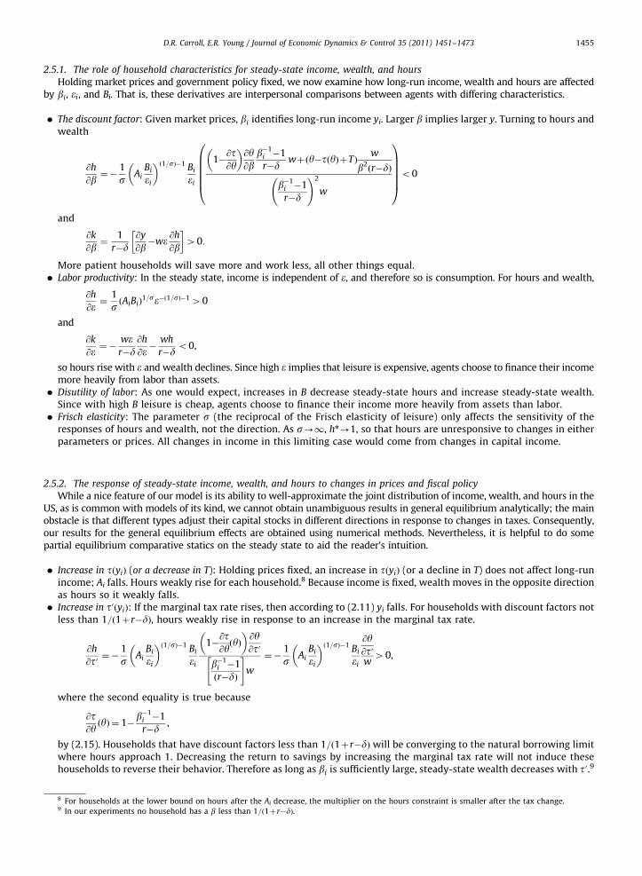
2.5.1. The role of household characteristics for steady-state income, wealth, and hours

Holding market prices and government policy fixed, we now examine how long-run income, wealth and hours are affectedby bi, ei, and Bi. That is, these derivatives are interpersonal comparisons between agents with differing characteristics.

�
The discount factor: Given market prices, bi identifies long-run income yi. Larger b implies larger y. Turning to hours andwealth
@h

@b¼�

1

s AiBi

ei

� �ð1=sÞ�1 Bi

ei

1�@t@y

� �@y@b

b�1i �1

r�dwþðy�tðyÞþTÞ

w

b2ðr�dÞ

b�1i �1

r�d

!2

w

0BBBBB@

1CCCCCAo0

and

@k

@b¼

1

r�d@y

@b�we @h

@b

� �40:

More patient households will save more and work less, all other things equal.
� Labor productivity: In the steady state, income is independent of e, and therefore so is consumption. For hours and wealth,
@h

@e¼

1

sðAiBiÞ

1=se�ð1=sÞ�140

and

@k

@e ¼�wer�d

@h

@e�wh

r�do0,

so hours rise with e and wealth declines. Since high e implies that leisure is expensive, agents choose to finance their incomemore heavily from labor than assets.
� Disutility of labor: As one would expect, increases in B decrease steady-state hours and increase steady-state wealth.
Since with high B leisure is cheap, agents choose to finance their income more heavily from assets than labor.
� Frisch elasticity: The parameter s (the reciprocal of the Frisch elasticity of leisure) only affects the sensitivity of the
responses of hours and wealth, not the direction. As s-1, hn-1, so that hours are unresponsive to changes in eitherparameters or prices. All changes in income in this limiting case would come from changes in capital income.

2.5.2. The response of steady-state income, wealth, and hours to changes in prices and fiscal policy

While a nice feature of our model is its ability to well-approximate the joint distribution of income, wealth, and hours in theUS, as is common with models of its kind, we cannot obtain unambiguous results in general equilibrium analytically; the mainobstacle is that different types adjust their capital stocks in different directions in response to changes in taxes. Consequently,our results for the general equilibrium effects are obtained using numerical methods. Nevertheless, it is helpful to do somepartial equilibrium comparative statics on the steady state to aid the reader’s intuition.

�
Increase in tðyiÞ (or a decrease in T): Holding prices fixed, an increase in tðyiÞ (or a decline in T) does not affect long-runincome; Ai falls. Hours weakly rise for each household.8 Because income is fixed, wealth moves in the opposite directionas hours so it weakly falls. � Increase in t0ðyiÞ: If the marginal tax rate rises, then according to (2.11) yi falls. For households with discount factors not
less than 1=ð1þr�dÞ, hours weakly rise in response to an increase in the marginal tax rate.

@h

@t0 ¼ �1

s AiBi

ei

� �ð1=sÞ�1 Bi

ei

1�@t@yðyÞ

� �@y@t0

b�1i �1

ðr�dÞ

" #w

¼�1

s AiBi

ei

� �ð1=sÞ�1 Bi

ei

@y@t0w

40,

where the second equality is true because

@t@yðyÞ ¼ 1�

b�1i �1

r�d,

by (2.15). Households that have discount factors less than 1=ð1þr�dÞ will be converging to the natural borrowing limitwhere hours approach 1. Decreasing the return to savings by increasing the marginal tax rate will not induce thesehouseholds to reverse their behavior. Therefore as long as bi is sufficiently large, steady-state wealth decreases with t0.9

8 For households at the lower bound on hours after the Ai decrease, the multiplier on the hours constraint is smaller after the tax change.9 In our experiments no household has a b less than 1=ð1þr�dÞ.


�
Increase in r: An increase in the steady-state rental rate leads to a rise in income for every household. The size of thisincrease for any given household will depend upon what part of the marginal tax function the household faces. In orderfor (2.11) to be satisfied for any particular household i, the after-tax return on savings in the new steady state must beequal to what it was in the initial steady state. Therefore, an r increase must be offset by an increase in t0ðyiÞ (i.e.,income must rise). If a particular household is in a region of the marginal tax function where its derivative is near zero(near the upper bound), then a large increase in yi will be necessary to satisfy (2.11). On the other hand, if the derivativeis large, then only a small increase in yi will restore equality in (2.11). Therefore, an increase in r will tend to increaseincome inequality.
In addition, the long run response of hours is weakly negative and that of long-run wealth is strictly positive. Puttingaside the trivial case where hours are 0 before and after the tax change

@h

@r¼

@ 1� AiBi

ei

� �1=s !

@r¼�

1

sAi

Bi

ei

� �ð1=sÞ�1 @Ai

@r

Bi

ei

� �o0:

Including households at the lower bound on hours, @h=@rr0. Since long-run income is unambiguously greater and laborincome is weakly decreasing, long-run wealth is a strictly increasing function of r. This result ensures that a steady stateexists.

3. Numerical experiments

In order to find quantitative results for the model, we conduct a series of revenue-neutral tax experiments. We selectthe following functional form for each household’s tax bill:

tðyÞ ¼ n0ðy�ðy�n1þn2Þ

�ð1=n1ÞÞþn3y:

The first term is the functional form Gouveia and Strauss (1994) assumed to estimate the effective personal income taxfunction using 1989 US tax return data.10 The second term, n3y, captures other tax revenues that are not modeled but are paidby households in the data (e.g., excise taxes, estate taxes, property taxes). In the interest of focusing on the progressivity of thepersonal income tax, the combined burden of these other taxes is assumed to be a linear function of income.

n0 sets the upper bound on the marginal personal income tax rate, with the highest possible value of t0ðyÞ being n0þn3.n1 changes the curvature of the function; the exact way in which it does so will be clear after the first experiment. Finally,n2 adjusts tðyÞ for the unit of measure of income. Throughout all experiments its value remains fixed. It is important toremember that because of revenue neutrality, the average tax rate is unchanged across experiments. The wide range ofsteady-state distributions and of their corresponding moments strongly suggests that ignoring the distributional effects oftax changes may not be innocuous.

We choose not to model labor income and capital income as separate tax bases for two reasons. First, this paper makescomparisons to other papers on tax reform which do not distinguish between these two bases. Second, because there is norisk in the model, the appropriate tax rates are those placed on income generated from (nearly) risk-free assets likeinterest on bank savings accounts, certificates of deposit, and government bonds. The US tax code, the code to which themodel is calibrated, does not subject these sources to capital gains taxation but rather to general income tax. We also donot attempt to decompose our results into the effects caused by altering the progressivity of capital income or laborincome separately. Our tax function is not additive, so that it is not possible to use separate tax functions for differentsources of income but keep the marginal tax schedule on total income the same as in the benchmark economy.

We do not compute transitional dynamics in our model. As the reader will see below, changes in progressivity havequantitatively large effects in our model, particularly for high-b types. These types also converge very slowly to their newsteady state, due to the relative flatness of the tax function they face. The implication is that transitions would beextremely lengthy and, given the number of different types we need to capture the joint distribution of hours, income, andwealth, would require far too much memory for even 64-bit addressing to handle. The length of the transition also impliesthat the reader should interpret our large effects as likely to arise in the very distant future, so that perhaps they do notseem unreasonable.

3.1. Calibration

To initialize the model, we calibrate to income, wealth, hours, and analysis weight data from the Survey of ConsumerFinances 1992, 1995, 1998, 2001, and 2004. The total number of households used for the experiment is 15,437. Afterdeflating the data by the 1992 GDP deflator, we normalize aggregate income to 1, wealth to 3, and hours to 0.33. We set

10 This functional form has been used in a number of quantitative studies of progressive taxation, including Castaneda et al. (1998), Conesa and

Krueger (2006), and Conesa et al. (2009). An alternative smooth specification is used in Sarte (1997), Li and Sarte (2003), and Carroll (2011), while a more

detailed nonsmooth function is used in Ventura (1999).

0.926

0.928 0.9

30.9

320.9

340.9

360.9

38 0.94

0.942

0.944

0.946

0

10

20

30

40

50

60

70

80

90

100

β

ε

Fig. 1. Calibrated discount factors and labor productivity values.


a¼ 0:36 and s¼ 2. Government spending is 20% of aggregate income and transfers are 10%. We also fix n0 and n1 to 0.258 and0.768 as estimated by Gouveia and Strauss (1994). We set the remaining parameters, so that the steady state of our modelmatches specific aggregate statistics at the annual frequency. n3 ¼ 0:0855 which implies that 71.5% of tax revenue is raisedthrough the progressive personal income tax.11 Depreciation is set to d¼ 0:05, so that investment is 15% of income. ci for eachhousehold is set to the household’s population weight in the SCF. We then normalize these weights, so that

Pici ¼ 1.

fbi,ei,Big, r, and n2 are solved for jointly. The preference parameters are backed out from the first-order conditions anddefinition of income for each household. A difficulty with this method arises when a survey household works zero hours.Because the intratemporal condition is not binding there are infinitely many possible solutions to the system. Specifically,it is impossible to back out ei and Bi directly. To address this problem, we first solve for the household characteristics ofworking households and regress in logs ei on age, education, and race (reported in the survey). In addition, we constructthe cdf of B. Then if we encounter a non-working household, we use its reported age, education, and race along with theregression equation to get a predicted ei. Given ei, we find the value Bi,min for which the nonnegativity constraint on hoursis just binding (the constraint binds and the multiplier is zero). To select a Bi we draw from the cdf of B truncated below atBi,min. Finally, r and n2 are adjusted to clear the market for capital goods and the government budget constraint. We ignoresolutions on the downward sloping side of the Laffer curve.

The scatter plots in Figs. 1–3 display the relationship between the calibrated values for preferences and laborproductivities. Looking first across discount factors, the model is backing out from the data a nonlinear relationshipbetween b and the other characteristics. Although e tends to rise with b at low b-values, there is a very sharp increase inthe observed productivities among the most patient households. This is due to the shape of the marginal tax function.Because it becomes relatively flat at high levels of income, large variation in income at the upper end will map into nearlythe same marginal tax rates. Since the marginal tax rates identify b through the Euler equation, these households will havediscount factors that are almost, though not exactly, equal. Even though these households do not vary much in terms ofdiscount factors, they do vary greatly in their labor productivity because of large differences in individual wealth and hoursworked. These differences show up in e and B.

It is important to note that the scatter plots in Figs. 1–3 do not take into account the population weights of the households. InTable 2, we report the mean values b, e, and B, and, because of the clear nonlinear relationship between some of theseparameters, the cross-correlations of their logs weighted by population. The numbers confirm the relationships that we wouldexpect. Labor productivity is positively correlated with discount factors which can be directly interpreted as high-incomehouseholds also tend to have high salaries. Labor disutility is negatively correlated with b, implying that high-income households

11 This is the average fraction of tax revenue from personal income taxes for the years 1992–2004. Our measure is taken from the Office of

Management and Budget Historical Table 2.2. We do not include Social Insurance and Retirement Receipts in our calculation, so we exclude FICA taxes.

0.926

0.928 0.9

30.9

320.9

340.9

360.9

38 0.94

0.942

0.944

0.946

0

20

40

60

80

100

120

140

160

180

200

β

B

Fig. 2. Calibrated discount factors and labor disutility values.

0 5 10 15 20 25 30 35 40 45 500

20

40

60

80

100

120

140

160

180

ε

B

Fig. 3. Calibrated labor productivity and labor disutility values.


are on average more willing to work all other things being equal. Finally, labor productivity and labor disutility are modestlypositively correlated, because there is a positive correlation in the data between income and wealth but a negative correlationbetween hours and wealth. Households with high income tend to have high e values, but do not work that much more onaverage than low-income households, which the model matches by assigning to these households a relatively high value for B.

3.1.1. A note on the measurement of tax progressivity

We now discuss the measurement of progressivity. It is not clear exactly how to characterize a tax change as‘‘progressive’’ or ‘‘regressive’’ when the underlying distribution of income changes. As a result, it is not straightforward tocompare the progressiveness of two tax functions and so there are several methods used in the literature, and these

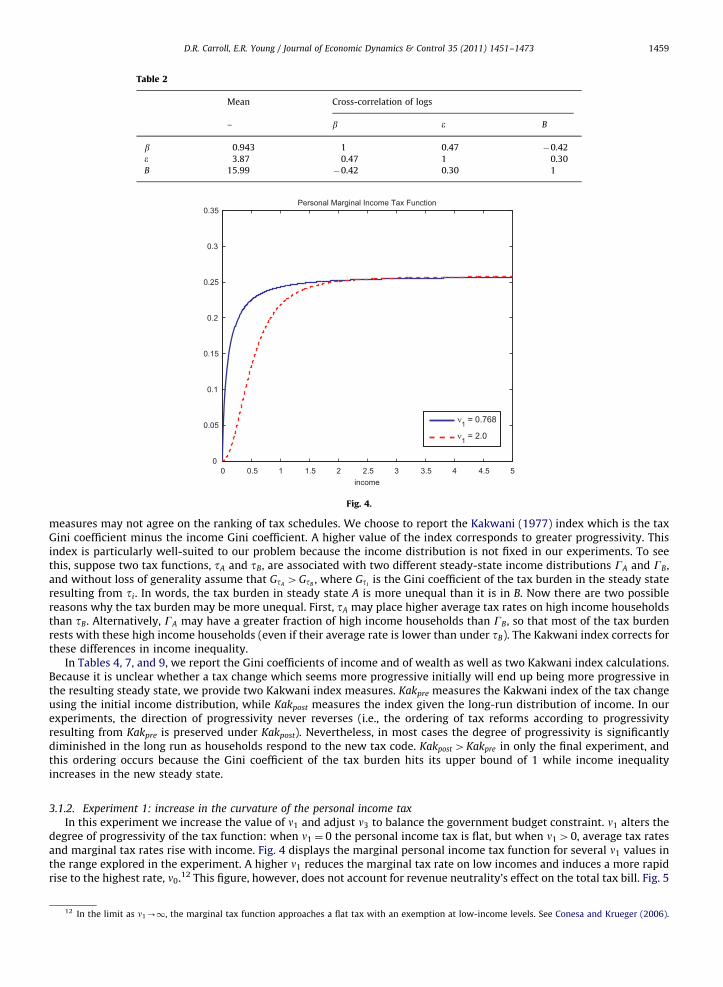
Table 2

Mean Cross-correlation of logs

– b e B

b 0.943 1 0.47 �0.42

e 3.87 0.47 1 0.30

B 15.99 �0.42 0.30 1

0 0.5 1 1.5 2 2.5 3 3.5 4 4.5 50

0.05

0.1

0.15

0.2

0.25

0.3

0.35

income

Personal Marginal Income Tax Function

ν1 = 0.768

ν1 = 2.0

Fig. 4.


measures may not agree on the ranking of tax schedules. We choose to report the Kakwani (1977) index which is the taxGini coefficient minus the income Gini coefficient. A higher value of the index corresponds to greater progressivity. Thisindex is particularly well-suited to our problem because the income distribution is not fixed in our experiments. To seethis, suppose two tax functions, tA and tB, are associated with two different steady-state income distributions GA and GB,and without loss of generality assume that GtA

4GtB, where Gti

is the Gini coefficient of the tax burden in the steady stateresulting from ti. In words, the tax burden in steady state A is more unequal than it is in B. Now there are two possiblereasons why the tax burden may be more unequal. First, tA may place higher average tax rates on high income householdsthan tB. Alternatively, GA may have a greater fraction of high income households than GB, so that most of the tax burdenrests with these high income households (even if their average rate is lower than under tB). The Kakwani index corrects forthese differences in income inequality.

In Tables 4, 7, and 9, we report the Gini coefficients of income and of wealth as well as two Kakwani index calculations.Because it is unclear whether a tax change which seems more progressive initially will end up being more progressive inthe resulting steady state, we provide two Kakwani index measures. Kakpre measures the Kakwani index of the tax changeusing the initial income distribution, while Kakpost measures the index given the long-run distribution of income. In ourexperiments, the direction of progressivity never reverses (i.e., the ordering of tax reforms according to progressivityresulting from Kakpre is preserved under Kakpost). Nevertheless, in most cases the degree of progressivity is significantlydiminished in the long run as households respond to the new tax code. Kakpost 4Kakpre in only the final experiment, andthis ordering occurs because the Gini coefficient of the tax burden hits its upper bound of 1 while income inequalityincreases in the new steady state.

3.1.2. Experiment 1: increase in the curvature of the personal income tax

In this experiment we increase the value of n1 and adjust n3 to balance the government budget constraint. n1 alters thedegree of progressivity of the tax function: when n1 ¼ 0 the personal income tax is flat, but when n140, average tax ratesand marginal tax rates rise with income. Fig. 4 displays the marginal personal income tax function for several n1 values inthe range explored in the experiment. A higher n1 reduces the marginal tax rate on low incomes and induces a more rapidrise to the highest rate, n0.12 This figure, however, does not account for revenue neutrality’s effect on the total tax bill. Fig. 5

12 In the limit as n1-1, the marginal tax function approaches a flat tax with an exemption at low-income levels. See Conesa and Krueger (2006).

0 0.5 1 1.5 2 2.5 3 3.5 4 4.5 50.05

0.1

0.15

0.2

0.25

0.3

0.35

0.4Total Marginal Tax Function

ν1 = .768

ν1 = 2.0

Fig. 5.

Table 3Percentage change in aggregate values.

Experiment 1: % change

Y K C H N

n1 ¼ 0:768 – – – – –

n1 ¼ 1:0 17.4 21.1 21.7 �11.4 16.1

n1 ¼ 2:0 37.6 41.1 47.0 �27.6 36.4

n1 ¼ 3:0 41.7 43.0 52.2 �29.4 41.3


shows the marginal tax bill function which reflects the changes both in n1 and n3. When revenue neutrality is imposed it isnot immediately clear which tax is more progressive. A n1 of 0.768 places a higher total marginal tax rate on low incomethan greater n1 values do. It should be stressed that due to general equilibrium effects on tax revenue, the steady-statemarginal tax function after the policy change may imply lower marginal tax rates on all households, due to the adjustmentof n3 required to clear the government budget constraint. Since this reduction occurs over a (potentially) long transition,some households do face increased marginal tax rates initially as shown in Fig. 4.13

Turning to the effects of tax policy changes on the long-run levels of aggregate variables. We report the percentagechanges in the aggregates in Table 3. n1 has a hump-shaped relationship with income, capital, labor input, and wages. Fig. 6plots the steady-state levels of aggregate income, capital and consumption over n1. All three exhibit dramatic responses tochanges in n1. For example, increasing n1 from 0.768 to 2.0 causes aggregate wealth to increase by 41.1%. Even at thehighest value of n1, capital is still 43% above the baseline level. Responses in the labor market are plotted in Fig. 7, averagehours decline by as much as 29.4% meaning that higher progressivity in the personal income tax causes a substitution inproduction from less-productive to more-productive households. Interestingly, this pattern persists at high values of n1

even though the average wage falls sharply in this region. The large increase in labor input comes from the upper 4% ofproductive households. Figs. 8 and 9 plot the average hours within each percentile of the e-distribution for the baselineand n1 ¼ 2:0 cases. Notice that hours fall for nearly the entire economy, rising somewhat only at the upper end. Clearly

13 We investigate a log-linear approximation to the resulting steady-state outcomes of our policy experiments and in each case find local saddle

stability in the face of very highly persistent small shocks to n0 and n1. We cannot prove or demonstrate numerically that our model converges to a new

steady state for truly permanent large changes in the tax parameters, but based on related results in Carroll (2011) for a model with inelastic labor supply

we conjecture that it will converge monotonically, but slowly.

0.5 1 1.5 2 2.5 30.8

1

1.2

1.4

1.6

ν1

Income

0.5 1 1.5 2 2.5 32

3

4

5

ν1

Wealth

0.5 1 1.5 2 2.5 30.5

1

1.5

ν1

Consumption

Fig. 6. The response of aggregate variables to changes in progressivity.


average hours fall, but the impact on labor input of the upper 4% is much more significant. To make this point more clearly,we plot the average labor input within each percentile of e in Figs. 10 and 11. Now the difference at the upper tail is starklyapparent, especially in the top 1%. Even within the top 1%, positive association between hours and labor efficiency isevident. Notice that labor input for this group increases by an even larger proportion than its hours. The more-productivehouseholds in this group increase their hours more relative to the less productive.

One advantage of the modeling technique used here is the ability to characterize behavior at the extremes of theincome and wealth distributions. Figs. 12 and 13 show the breakdown in income and wealth across the steady-statedistribution for some values of n1. There are several conclusions that can be made about n1 increases. First, increasing n1

reduces income inequality. The Gini coefficient of income is cut by more than 50% when n1 increases from its baseline to3.0. In general this decline is caused because low and middle-income households’ marginal total tax rates are reduced themost. However, not all high income households reduce their income. Finally, the interest rate is lower in the n1 ¼ 3:0steady state. As discussed previously, this reduction leads to lower income inequality. Wealth inequality, on the otherhand, increases. Plots of the income, wealth, and tax burden Gini coefficients across steady states are shown in Fig. 14, andsummary statistics for this case are presented in Table 4.

For comparison purposes, we also compute this experiment using T to clear the government budget constraint insteadof n3; this experiment disentangles the pure progressivity effect from the required change in the flat tax rate. Table 5contrasts the results from the two experiments a specific value of n1 (it turns out that computing the new steady state issignificantly more difficult in the case, for reasons that are unclear to us, so we concentrate on the case with the largest n1

that we were able to solve). It is clear that this change has little impact on our results; the only difference is a slightlylarger decline in income inequality and a corresponding slightly larger increase in wealth inequality. Tax revenue isincreased by roughly 15% (about 4% of initial GDP), which generates the increase in T, and the aggregate quantities ofincome and wealth are not substantially different.

0.5 1 1.5 2 2.5 30.2

0.25

0.3

0.35

0.4

ν1

Hours

0.5 1 1.5 2 2.5 3

0.650.7

0.750.8

0.850.9

0.95

ν1

Labor Input

0.5 1 1.5 2 2.5 31.09

1.1

1.11

1.12

1.13

1.14

ν1

Wages



3.1.3. Experiment 2: shift between personal income taxation and other tax sources

This experiment increases the fraction of tax revenue raised with the progressive income tax relative to the flat tax byincreasing n0 and reducing n3. Figs. 15 and 16 compare the baseline marginal personal income tax functions and marginaltax bill functions for several values of n0 in the experiment.14 As n0 increases the marginal personal tax function rotatesupward, however, the marginal total tax function rotates downward which is consistent with our finding from theprevious experiment that higher progressivity is associated with more aggregate activity. In fact, in the steady state wheren3 ¼ 0, aggregate income is 11.6% larger and the capital stock is 14.5% larger than in the baseline case. Percent changes forall aggregates are displayed in Table 6. In Figs. 17 and 18, the steady-state values of the economy’s aggregates are plottedfor the whole range of n0 in the experiment. There is basically a linear relationship between n0 and the aggregate variables.As in Experiment 1 (though to a lesser degree), average hours falls and total labor input rises so once again moreprogressivity is effecting a substitution from less productive workers to more-productive workers.

The qualitative results for inequality are also similar to those from Experiment 1. Fig. 19 plots the steady-state Ginicoefficients of income, wealth, and taxes. The income Gini falls slightly as the total tax schedule tilts towards theprogressive income tax schedule. In contrast, wealth inequality rises significantly (roughly 16%). In this case, the largeincrease in wealth inequality comes primarily from large negative asset positions taken by moderately patient householdswith very high labor productivity. Summary statistics on inequality are presented in Table 7.

As above, we compare the results to a case where the transfer adjusts to clear the government budget constraint.Table 5 shows that the same results obtain here as in Experiment 1: income inequality falls a little more and wealthinequality rises a little more, with little difference in aggregates from the case where n3 adjusts.

14 At n0 ¼ 0:32, n3 � 0.

0 10 20 30 40 50 60 70 80 90 1000

0.05

0.1

0.15

0.2

0.25

0.3

0.35

0.4

0.45

0.5Hours across ε by Percentile

ν1 = 0.768

Fig. 8.

0 10 20 30 40 50 60 70 80 90 1000

0.05

0.1

0.15

0.2

0.25

0.3

0.35

0.4

0.45

0.5

ν1 = 2

Hours across ε by Percentile

Fig. 9.

0 10 20 30 40 50 60 70 80 90 1000

5

10

15

20

25

30

35

40

Effective Labor across ε by Percentile

ν1 = 0.768

Fig. 10.


0 10 20 30 40 50 60 70 80 90 1000

5

10

15

20

25

30

35

40

Effective Labor across ε by Percentile

ν1 = 2.0

Fig. 11.

0 10 20 30 40 50 60 70 80 90 1000

5

10

15Income Distribution by Percentile

0 10 20 30 40 50 60 70 80 90 1000

5

10

15

ν1 = 0.768

ν1 = 2.0

Fig. 12.


3.1.4. Experiment 3: flat tax with an exemption

In our final experiment, we consider a tax function like that from Conesa and Krueger (2006) who find that the optimalprogressive income tax combines a flat tax with an exemption level for income (we make no claims here about theoptimality of this change). In our case, this function is approximated by letting n1-1.15 In keeping with that paper weeliminate the linear schedule (i.e., n3 ¼ 0) and adjust n0 to balance the government’s budget. There are two marginal taxrates under this system — one is zero and the other is t ¼ n0, with a level of income y ¼ 1 that determines the switch.Incomes above y pay a tax bill tny, while incomes below y pay nothing.

15 Technically, the limiting marginal tax function maps y¼1 to tyð1Þ ¼ n0n2=ð1þn2Þ. With the exception of this single point, the limiting marginal tax

function and the two-step function used in this experiment are identical.

0 10 20 30 40 50 60 70 80 90 100−50

0

50

100Wealth Distribution by Percentile

0 10 20 30 40 50 60 70 80 90 100−50

0

50

100

ν1 = 0.768

ν1 = 2.0

Fig. 13.

0.5 1 1.5 2 2.5 30.2

0.3

0.4

0.5

0.6

0.7

0.8

0.9

1

ν1

Gini Coefficient

income wealth tax bill

Fig. 14. The response of inequality to progressivity.

Table 4

Experiment 1: inequality and progressivity

Gy Gk Kakpre Kakpost

v1¼0.768 49.4 74.5 0.045 0.045

v1¼1.0 41.6 85.2 0.075 0.064

v1¼2.0 26.3 88.9 0.144 0.095

v1¼3.0 23.8 93.4 0.165 0.118


Table 5

Aggregate income, wealth and inequality

(Y and K reported as percentage changes from initial steady state)

n3 T

Y K Gy Gk Y K Gy Gk

v1¼1.5 34 39 31.9 87.9 36 36 31.0 88.8

v0¼0.28 4 5 48.2 81.0 6 4 47.3 85.5

0 0.5 1 1.5 2 2.5 3 3.5 4 4.5 50

0.05

0.1

0.15

0.2

0.25

0.3

0.35

income

Personal Marginal Income Tax Function

ν0 = .258 ν0 = .280 ν0 = .320

Fig. 15.


Proposition 3.1. Given the tax function described above and a set of types each with a discount factor from fb1,b2, . . . ,bNg,where 14b14b24 � � �4bN 40, in any steady state with positive government expenditures

b2r1þð1�tÞðr�dÞ

1þr�db1:

Further, any type with discount factor b1 has income y141. Types with discount factors less than b2 have income equal to �T.

Any type with discount factor b2 will have y2r1.

Proof. A necessary condition for a steady state is that

1Zbn½1þð1�tyðynÞÞðr�dÞ� 8n, ð3:1Þ

where

tyðyÞ ¼0 if yr1,

t40 if y¼ 1:

(

First, from the household’s budget constraint any type n with assets approaching the borrowing limit must have steady-state income approaching �T. Thus if yn4�T

1¼ bn½1þð1�tyðyÞÞðr�dÞ�:

0 0.5 1 1.5 2 2.5 3 3.5 4 4.5 50

0.05

0.1

0.15

0.2

0.25

0.3

0.35

Total Marginal Tax Function

income

η0 = 0.258 η0 = 0.280 η0 = 0.320

Fig. 16.

Table 6Percentage change in aggregates.


Y K C H N

n0 ¼ 0:258 – – – – –

n0 ¼ 0:27 1.3 2.7 2.0 �2.6 0.7

n0 ¼ 0:29 5.1 7.5 6.8 �4.6 4.2

n0 ¼ 0:32 11.6 14.5 13.9 �7.3 9.4

0.26 0.27 0.28 0.29 0.3 0.31 0.32

1

1.05

1.1

1.15Income

0.26 0.27 0.28 0.29 0.3 0.31 0.322.8

3

3.2

3.4

Wealth

0.26 0.27 0.28 0.29 0.3 0.31 0.320.75

0.8

0.85

0.9

ν0

Consumption



0.26 0.27 0.28 0.29 0.3 0.31 0.320.3

0.31

0.32

0.33Hours

0.26 0.27 0.28 0.29 0.3 0.31 0.320.65

0.7

0.75Labor Input

0.26 0.27 0.28 0.29 0.3 0.31 0.321.08

1.1

1.12

ν0

Wage


0.26 0.27 0.28 0.29 0.3 0.31 0.320.45

0.5

0.55

0.6

0.65

0.7

0.75

0.8

0.85

0.9

ν0

Gini Coefficients

income wealth tax bill

Fig. 19. The response of inequality to progressivity.

Table 7



n0 ¼ 0:258 49.4 74.5 0.045 0.045

n0 ¼ 0:27 48.6 78.6 0.049 0.048

n0 ¼ 0:29 47.8 82.8 0.054 0.052

n0 ¼ 0:32 46.7 86.5 0.064 0.058



Second, since government expenditures are positive by budget balance tyðyÞ ¼ t for at least one type, implying that thereare households with income greater than 1 in the steady state. The steady-state Euler equation for any such household is

1¼ bn½1þð1�tÞðr�dÞ�:

Given r and t, this condition can only be satisfied for one bn. It is easy to see that this bn ¼ b1. If it were satisfied for someother bn, then

1ob1½1þð1�tyðyÞÞðr�dÞ�,

which violates (3.1). Therefore

1¼ b1½1þð1�tÞðr�dÞ�

and

14bn½1þð1�tÞðr�dÞ�, n41:

Note that (3.1) is satisfied for n41 when

bnr1þð1�tÞðr�dÞ

1þr�db1,

implying

bnr1

1þr�d:

To complete the proof, we will now show that a steady state cannot exist for bnZ ð1þð1�tÞðr�dÞÞb1=ð1þr�dÞ. Assumenot. Then there must exist a bs such that

bs ¼ Z1

1þr�d

� �þð1�ZÞ 1

1þð1�tÞðr�dÞ

� �, 0oZo1:

Either ysr1 or ys41. If ysr1, then

1Zbs½1þr�d�Z Z 1

1þr�d

� �þð1�ZÞ 1


� �� ½1þr�d�Z

Zð1þð1�tÞðr�dÞÞþð1�ZÞð1þr�dÞ1þð1�tÞðr�dÞ

1þð1�tÞðr�dÞZZð1þð1�tÞðr�dÞÞþð1�ZÞð1þr�dÞð1�ZÞð1þð1�tÞðr�dÞÞZ ð1�ZÞð1þr�dÞ,

which is a contradiction because t40. Therefore ys41, and

1¼ Z 1

1þr�d

� �þð1�ZÞ 1


� �� ½1þð1�tÞðr�dÞ� ¼ Z½1þð1�tÞðr�dÞ�þð1�ZÞð1þr�dÞ

1þr�d1þr�d¼ Z½1þð1�tÞðr�dÞ�þð1�ZÞð1þr�dÞZð1þr�dÞ ¼ Z½1þð1�tÞðr�dÞ�,

which is also a contradiction. Therefore ys does not exist implying that there can be no bs in a steady state.

Define an intermediate b type as any type n for which

b1½1þð1�tÞðr�dÞ�1þr�d

obnob1:

As shown above, the existence of an intermediate b type rules out a steady state. To see this, note that y¼1 is the onlypotential steady-state income value for any intermediate b type. At y¼1, however, consumption growth must be positivebecause this type discounts the future less than the market pays for deferred consumption (bn41=ð1þr�dÞ) so incomerises. Any increase in income discontinuously increases the marginal tax rate, so that the market no longer sufficientlyrewards this type for postponing consumption. Consumption growth will be less than one so income will fall. If thenumber of intermediate b types is greater than 1, then the most patient of them will have the largest consumption growthin the initial period and will converge the slowest back toward an income of 1.

The wealth distribution in this case would have the most patient type holding the largest share of wealth (possibly anextremely large share). Intermediate b types could have positive or negative wealth depending upon their labor income.All other types have assets approaching the natural borrowing limit (meaning their consumption and leisure bothapproach zero). We find that intermediate types exist in our calibrated economy, thus the reported findings for thisexperiment are not from a steady state. They should be interpreted instead as reporting features of an economy with ajoint income and wealth distribution that is (not quite) the limiting distribution from the sequence of steady statesassociated with a sequence of n1 as n1 approaches infinity.

In the (limiting) steady state of our numerical experiment, t ¼ 14:5%. Table 8 reports the percentage changes in the steadystate aggregates. Aggregate income rises by 203% while the capital stock increases by 266%. The extreme rise in these values iscaused almost entirely by the behavior of the most patient household. This household has income equal to 40,672 times the

Table 8


Y K C H N

n1 ¼ 0:768 – – – – –

v1 ¼1 203.2 265.6 254.0 10.6 184.5

Table 9



n1 ¼ 0:768 49.4 74.5 0.045 0.045

v1 ¼1 69.8 1.0 0.284 0.302


average and wealth equal to 166,512 times the average.16 Hours increase only 11%, but total labor input surges by 185%. Thebig increase in labor input is not caused by the most patient household but rather by the highly productive among the otherhouseholds. Hours for these households rise in response to a zero tax rate, leading to large increases in labor income. Tomaintain an income level below y, this additional labor income is balanced by very large negative asset positions. Withhouseholds in this economy taking such extreme positions, it is not surprising that inequality increases significantly. The Ginicoefficient of income rises by 41.4% to 0.7, and the Gini coefficient of wealth rises from 0.745 to nearly 1. The extremeinequality that results from this experiment is consistent with known results regarding models with heterogeneous discountfactors and no taxation, such as Becker (1980) and Smith (2009): every type except the most patient converges to the lowerbound on consumption. Table 9 presents the summary statistics on inequality.

3.2. Explanation of results

In all three cases, increasing the progressivity of the tax schedule leads to increases in aggregate capital, aggregate laborinput, and, as a consequence, aggregate income. At first, this result seems surprising given that a more progressive taxplaces a relatively heavier tax burden upon the wealthy. The key is that since the income tax falls on both means of income(capital and labor) households cannot avoid taxes by changing the source of their income. For a given tax policy, eachhousehold’s long run total income is set by its discount factor and the rate of return on savings. The only thing to beresolved is the composition of long run income between labor income and capital income.17

3.2.1. Change in hours

As shown above, long-run hours for a household i are determined by the following equation:

hi ¼

0 if Ai4ei

Bi,

1� AiBi

ei

� �1=sotherwise,

8>>><>>>:

where

Ai ¼ci

ð1�t0ðyiÞÞw¼

yi�tðyiÞþT

ðb�1i �1Þ

w

r�d

:

Since Bi=ei is fixed for the household, the direction of its labor response to tax reform depends only on Ai. If Ai increases(decreases), then hours fall (rise). In words, Ai is the ratio of the long-run disposable income of household i to the long-runfactor price ratio scaled by the household’s rate of time preference. The numerator captures the wealth effect (if disposableincome increases, then all else equal hours decline) while the denominator is the substitution effect (all else equal a rise in

16 To give some perspective to this number, the average wealth in the US is around $180,000 (inclusive of illiquid retirement portfolios and housing).

Our wealthiest household therefore has a wealth of nearly $30 billion. Currently there are only three individuals on the Forbes’ billionaires list with total

wealth greater than $30 billion.17 The explanations in the following subsections are specific to the numerical experiments above. Assumptions regarding the directions of changes in

aggregate variables are consistent with their changes in the experiments. The following explanations should not be considered a rigorous analytical study

of general equilibrium in the model. As discussed above, such a general equilibrium study would not deliver unambiguous analytical results. For instance,

because household types respond to tax changes in opposite ways, any results conclusions about the impact on aggregate variables would depend

critically upon the relative measure of those types as well as the strength of their responses.


the wage relative to the return on capital causes hours to rise). The rate of time preference b�1�1 makes the wealth effect

relatively more important for highly patient households. The magnitude by which hours move depends both upon the sizeof the change in Ai and the ratio of labor disutility to labor effectiveness. A household that is highly productive relative toits disutility for labor will change hours less. Clearly, if this ratio is very small then the household will not work at all.

The fact that highly patient (or equivalently, high income) households place more importance on the wealth effect,along with strong tendency for the very highly productive to have high income, explains why aggregate effective laborinput rises even though average hours falls. Making the tax code more progressive causes the income distribution to shrinkinward. Income rises for the poor and middle-class causing them to work less. At the same time income for the rich falls.Because the wealth effect is particularly strong for them, their hours increase. Although, on average the rich tend to havelower Bi=ei, the dampening effect this heterogeneity produces only partially mitigates their rise in hours. Moreover, againbecause they tend to be highly productive workers, the positive labor response induces a large upward movement ineffective labor input.18

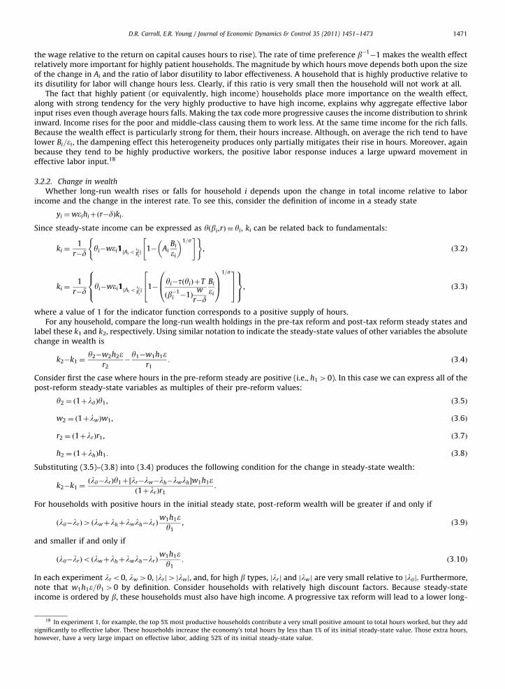
3.2.2. Change in wealth

Whether long-run wealth rises or falls for household i depends upon the change in total income relative to laborincome and the change in the interest rate. To see this, consider the definition of income in a steady state

yi ¼weihiþðr�dÞki:

Since steady-state income can be expressed as yðbi,rÞ � yi, ki can be related back to fundamentals:

ki ¼1

r�dyi�wei1fAi o

eiBig

1� AiBi

ei

� �1=s" #( )

, ð3:2Þ

ki ¼1

r�dyi�wei1fAi o

eiBig

1�yi�tðyiÞþT

ðb�1i �1Þ

w

r�d

Bi

ei

0B@

1CA

1=s264

375

8><>:

9>=>;, ð3:3Þ

where a value of 1 for the indicator function corresponds to a positive supply of hours.For any household, compare the long-run wealth holdings in the pre-tax reform and post-tax reform steady states and

label these k1 and k2, respectively. Using similar notation to indicate the steady-state values of other variables the absolutechange in wealth is

k2�k1 ¼y2�w2h2e

r2�y1�w1h1e

r1: ð3:4Þ

Consider first the case where hours in the pre-reform steady are positive (i.e., h140). In this case we can express all of thepost-reform steady-state variables as multiples of their pre-reform values:

y2 ¼ ð1þlyÞy1, ð3:5Þ

w2 ¼ ð1þlwÞw1, ð3:6Þ

r2 ¼ ð1þlrÞr1, ð3:7Þ

h2 ¼ ð1þlhÞh1: ð3:8Þ

Substituting (3.5)–(3.8) into (3.4) produces the following condition for the change in steady-state wealth:

k2�k1 ¼ðly�lrÞy1þ½lr�lw�lh�lwlh�w1h1e

ð1þlrÞr1:

For households with positive hours in the initial steady state, post-reform wealth will be greater if and only if

ðly�lrÞ4ðlwþlhþlwlh�lrÞw1h1ey1

, ð3:9Þ

and smaller if and only if

ðly�lrÞoðlwþlhþlwlh�lrÞw1h1ey1

: ð3:10Þ

In each experiment lr o0, lw40, jlrj4 jlwj, and, for high b types, jlrj and jlwj are very small relative to jlyj. Furthermore,note that w1h1e=y140 by definition. Consider households with relatively high discount factors. Because steady-stateincome is ordered by b, these households must also have high income. A progressive tax reform will lead to a lower long-

18 In experiment 1, for example, the top 5% most productive households contribute a very small positive amount to total hours worked, but they add

significantly to effective labor. These households increase the economy’s total hours by less than 1% of its initial steady-state value. Those extra hours,

however, have a very large impact on effective labor, adding 52% of its initial steady-state value.


run income for this group (i.e., lyo0) and as stated above the decline is large in magnitude relative to the decline in r.From the analysis above regarding hours, it is clear that hours will rise so lh40. Taken together, the signs of the l’s implythat (3.10) holds and so steady-state wealth falls within this group. By similar reasoning, nearly all low- and middle-income households increase their wealth because ly40, lho0, and lw and lr are relatively small in magnitude comparedto ly and lh. There is a very small measure of households in the upper-middle income region for which the lh � 0 andly � 0. Among these households wealth may rise or fall slightly depending upon the proportion of pre-reform labor incometo pre-reform total income.

Finally, turning to households which worked zero hours pre-reform

k2�k1 ¼ðly�lrÞy1�ð1þlwÞw1h2e

ð1þlrÞr1:

Again, from examining the hours supply decision, households for which h240 must experience sufficiently largemovements in disposable income. In our experiments this large change never occurs, so that hours before and after thereform remain zero. This result should not be surprising given that few high-income households supply zero hours in thepre-reform steady state, and our method for choosing B is unlikely to produce households that are marginal with respect totheir hours choice. Since h2¼0 is the relevant case, whether wealth rises or falls after reform for any household dependsupon the sign of ly (because lr o0). Only a very small measure of high-income households with no labor income decreasewealth. All other zero hours households increase their wealth. In general, because the marginal tax function is much flatterat high levels of income, the change in yi will be larger in magnitude for the rich and thus so will the change in wealth.That said, because the income distribution is skewed, the rich make up a small fraction of the total economy. On net, in allof our experiments the dissaving of the rich is more than offset by the saving of other households.

4. Conclusion

In this paper we have investigated the consequences of altering the progressivity of the tax code in a model withheterogenous household but no idiosyncratic risk. As we noted in the Introduction, our results are qualitatively differentfrom those found in models with incomplete asset markets, as well as quantitatively. Thus, we argue that more attentionmust be paid to derive the insurance opportunities available to households, either in terms of borrowing limits or missinginsurance markets. Some papers take steps in this direction, such as Krueger and Perri (2011) or Abraham and Carceles-Poveda (2009), but more work is needed.

We want to point out ‘‘progressive’’ tax reforms – that is, changes in the tax function that induce more progressivityrelative to the estimated U.S. tax function – would enjoy strong political support. Carroll (2011) investigates the source forthis support; it would be of considerable interest to investigate this issue in the models that endogenize risk sharing. Itwould also be of interest to extend the results from Davila et al. (2005) and Athreya et al. (2009) regarding the constrainedefficient allocations to the model considered here.

Acknowledgments

We would like to thank the participants of the Conference in Honor of Steve Turnovksy in Vienna for comments,particularly our discussant Timo Trimborn and the editor Ken Kletzer. Young thanks the Bankard Fund for PoliticalEconomy at the University of Virginia for financial support. All errors are our responsibility. The opinions expressed hereare those of the authors only and do not reflect the positions of the Federal Reserve Bank of Cleveland or the FederalReserve System.

References

Abraham, A., Carceles-Poveda, E., 2009. Tax reform with endogenous borrowing limits and incomplete markets. mimeo.Aiyagari, S.R., 1994. Uninsured idiosyncratic risk and aggregate saving. Quarterly Journal of Economics 109 (3), 659–684.Athreya, K, Tam, X., Young, E.R., 2009. Constrained efficiency with idiosyncratic shocks and elastic labor supply. mimeo.Badel, A., Huggett, M. 2010. Interpreting life-cycle inequality patterns as an efficient allocation: mission impossible? Federal Reserve Bank of St. Louis

Working Paper 2010-046A. Federal Reserve Bank of St. Louis.Becker, R.A., 1980. On the long-run steady state in a simple dynamic model of equilibrium with heterogeneous households. Quarterly Journal of

Economics 95 (2), 375–382.Carroll, D.R., 2011. The demand for income tax progressivity in the growth model. Federal Reserve Bank of Cleveland Working Paper 1106, Federal

Reserve Bank of Cleveland.Carroll, D.R., Young, E.R., 2009. The stationary distribution of wealth under progressive taxation. Review of Economic Dynamics 12 (3), 469–478.Castaneda, A., Dıaz-Gimenez, J., Rıos-Rull, J.V., 1998. Earnings and wealth inequality and income taxation: quantifying the trade-offs of switching to a

proportional income tax in the U.S. Federal Reserve Bank of Cleveland Working Paper 9814. Federal Reserve Bank of Cleveland.Castaneda, A., Dıaz-Gimenez, J., Rıos-Rull, J.V., 2003. Accounting for wealth and income inequality. Journal of Political Economy 111 (4), 818–857.Conesa, J.C., Kitao, S., Krueger, D., 2009. Taxing capital: not a bad idea after all!. American Economic Review 99 (1), 25–48.Conesa, J.C., Krueger, D., 2006. On the optimal progressivity of the income tax. Journal of Monetary Economics 53 (7), 1425–1450.Davila, J., Hong, J.H., Krusell, P., Rıos-Rull, J.V., 2005. Constrained efficiency in the neoclassical growth model with uninsurable idiosyncratic shocks. PIER

Working Paper 05-023. Penn Institute for Economic Research, Department of Economics, University of Pennsylvania.


Dıaz-Gimenez, J., Pijoan-Mas, J., 2006. Flat tax reform in the U.S.: a boon for the income poor. CEPR Discussion Paper 5812. Centre for Economic PolicyResearch.

Gouveia, M., Strauss, R.P., 1994. Effective federal individual tax functions: an exploratory empirical analysis. National Tax Journal 47 (2), 317–339.Kakwani, N.C., 1977. Measurement of tax progressivity: an international comparison. Economic Journal 87 (345), 71–80.Krueger, D., Perri, F., 2011. Public versus private risk sharing. Journal of Economic Theory 146 (3), 92–956.Krusell, P., Mukoyama, T., S-ahin, A., Smith Jr., A.A., 2009. Revisiting the welfare effects of eliminating business cycles. Review of Economic Dynamics 12

(3), 393–404.Li, W., Sarte, P.D.G., 2003. Progressive taxation and long-run growth. American Economic Review 94 (5), 1705–1716.Meh, C., 2005. Entrepreneurship, wealth inequality, and taxation. Review of Economic Dynamics 8 (3), 688–719.Saez, E., 2002. Optimal progressive capital income taxes in the infinite horizon model. NBER Working Paper 9046, National Bureau of Economic Research.Sarte, P.D.G., 1997. Progressive taxation and income inequality in dynamic competitive equilibrium. Journal of Public Economics 66 (1), 145–171.Smith Jr., A.A., 2009. Comment on: ‘‘Welfare implications of the transition to high household debt’’ by Campbell and Hercowitz. Journal of Monetary

Economics 56 (1), 17–19.Ventura, G., 1999. Flat tax reform: a quantitative exploration. Journal of Economic Dynamics and Control 23 (9–10), 1425–1458.

the long run effects of changes in tax...

Documents