Journal of Econometrics 187 (2015) 580–592

Contents lists available at ScienceDirect

Journal of Econometrics

journal homepage: www.elsevier.com/locate/jeconom

The long and the short of the risk-return trade-off✩

Marco Bonomo a, René Garcia b,∗, Nour Meddahi c, Roméo Tédongap d

a Insper Institute of Education and Research, Brazilb Edhec Business School, Francec Toulouse School of Economics (GREMAQ, IDEI), Franced Stockholm School of Economics, Sweden

a r t i c l e i n f o

Article history:Available online 12 March 2015

JEL classification:G1G12G11C1C5

Keywords:Equilibrium asset pricingTime-aggregationRealized measures

a b s t r a c t

The relationship between conditional volatility and expected stock market returns, the so-called risk-return trade-off, has been studied at high- and low-frequency. We propose an asset pricing model withgeneralized disappointment aversion preferences and short- and long-run volatility risks that capturesseveral stylized facts associated with the risk-return trade-off at short and long horizons. Writing themodel in Bonomo et al. (2011) at the daily frequency, we aim at reproducing the moments of thevariance premium and realized volatility, the long-run predictability of cumulative returns by the pastcumulative variance, the short-run predictability of returns by the variance premium, as well as thedaily autocorrelation patterns at many lags of the VIX and of the variance premium, and the daily cross-correlations of these two measures with leads and lags of daily returns. By keeping the same calibrationas in this previous paper, we ensure that the model is capturing the first and second moments of theequity premium and the risk-free rate, and the predictability of returns by the dividend yield. Overalladding generalized disappointment aversion to the Kreps–Porteus specification improves the fit for boththe short-run and the long-run risk-return trade-offs.

© 2015 Elsevier B.V. All rights reserved.

1. Introduction

To study the relationship between conditional volatility andexpected stock market returns researchers have mainly runlinear regressions. The outcome after more than two decades ofempirical studies is rather disappointing. Some find a positive re-lation, others a negative one. Inmany studies, there is no significant

✩ An earlier version of this paper was presented at the Econometrics KnowledgePlatform 3rd Annual Workshop, Liverpool University Management School, Liver-pool, in April 2014 as well as at the SOFIE 7th Annual Conference, Rotman Schoolof Business, University of Toronto, Toronto, in June 2014. We thank participantsfor their comments. We also thank two referees and the editor for their useful andconstructive comments. This work was supported by grants FQRSC-ANR (ANR-11-FRQU-002-01 - DFAPRM -) to the second and third authors. NourMeddahi benefitedfrom the financial support of the chair ‘‘Marché des risques et création de valeur’’,Fondation du risque/SCOR, and from the European Communitys Seventh Frame-work Programme (FP7/2007–2013) Grant Agreement no. 230589.∗ Correspondence to: Edhec Business School, 393, Promenade des Anglais, BP

3116, 06202 Nice Cedex 3, France.E-mail addresses: MarcoACB@insper.edu.br (M. Bonomo),

rene.garcia@edhec.edu (R. Garcia), nour.meddahi@tse-fr.eu (N. Meddahi),romeo.tedongap@hhs.se (R. Tédongap).

http://dx.doi.org/10.1016/j.jeconom.2015.02.0400304-4076/© 2015 Elsevier B.V. All rights reserved.

trade-off.1 Several recent contributions have revived the de-bate. Bandi and Perron (2008) find that the dependence is statis-tically mild at short horizons, which explains the contradictingresults in the literature, but increases with the horizon and isstrong in the long run (between 6 and 10 years). A recent trendin the literature has also put forward the variance risk premium(VRP) as a strong predictor of stock returns in the short run (seein particular Bollerslev et al., 2009). Bollerslev et al. (2006) studythe relationship between volatility and past and future returnsin high-frequency equity market data. They find an asymmetricpattern in the cross-correlations between absolute high-frequencyreturns and current and past high-frequency returns. Correla-tions between absolute returns and past returns are significantly

1 In a survey about measuring and modeling variation in the risk-return trade-off, Lettau and Ludvigson (2010) attribute in large part the disagreement in theempirical literature on this relation to the limited amount of information generallyused to model the conditional mean and conditional volatility of excess stockmarket returns. Rossi and Timmermann (2010) argue that there is no theoreticalreason for assuming a linear relationship between the expected returns and theconditional volatility. They found support for nonlinear patterns in the risk-returntrade-off.

M. Bonomo et al. / Journal of Econometrics 187 (2015) 580–592 581

negative for several days, while the reverse cross-correlations be-tween absolute returns and future returns are negligible.

We propose an equilibrium consumption-based asset pricingmodel with generalized disappointment aversion preferences andvolatility risk to rationalize these recently put-forward stylizedfacts. We extend the model in Bonomo et al. (2011) in two ways.First, sincewewant to address short-run volatility-return relation-ship, we write the model at the daily frequency. Second, we add ashort-run volatility risk to the long-run volatility risk in Bonomoet al. (2011). Our main contribution is to reproduce relations be-tween returns and volatility at short and long horizons with anequilibrium model calibrated at a high-frequency daily level. Wecan then solve the model daily and construct realized quantitiesat lower frequencies. Thanks to Markov-switching fundamentals,a key advantage of the model proposed by Bonomo et al. (2011) isto find analytical formulas for moments of asset pricing quantitiessuch as payoff ratios and returns, and for coefficients of predictabil-ity regressions at any horizon. In this framework we are able toproduce analytical results at high frequency as in Bollerslev et al.(2006) together with the long-run regressions of Bandi and Perron(2008) in the same model. For generating empirical stylized facts,we keep the same calibration as in Bonomo et al. (2011) to makesure that the model produces first and second moments of price-dividend ratios and asset returns as well as return predictabilitypatterns in line with the data.

At the high-frequency level, we assess the capacity of themodelto reproduce the autocorrelation of daily returns, squared dailyreturns, and cross-correlations of daily returns and squared returnsat various leads and lags. We also build measures of monthlyrealized variance (RV) by summing daily squared returns andcompute moments of realized volatility. The variance premiumis obtained by first taking the expectation under the risk-neutralmeasure of this realized volatility and subtracting the latter fromthe obtained risk-neutral volatility. The predictability of returns bythe variance premium is then established for horizons of one totwelvemonths. At longer horizons,we reproduce the predictabilityregressions of Bandi and Perron (2008) by aggregating returns andvolatilities over periods of one to ten years.

With generalized disappointment aversion preferences, thestochastic discount factor (SDF) has a kink at a disappointingthreshold equal to a given fraction of the certainty equivalent oflifetime future utility. In regular disappointment aversion prefer-ences, the threshold is equal to the certainty equivalent. In themodel we propose, expected consumption growth is constant.Therefore, the only long-run risk is an economic uncertainty riskcaptured by the volatility of consumption. To capture a richershort-run dynamics in volatility and the predictability of returnsby the variance premium we add a short-lived volatility compo-nent to the persistent component that was used in Bonomo et al.(2011). Shocks in the high- and low-persistence components ofconsumption growth volatility affect the volatility of the SDF. Apersistent increase in consumption growth volatility increases thevolatility of future utility. A more volatile future utility increasesthe probability of disappointing outcomes, making the SDF morevolatile. In our model dividends share the consumption volatilityprocess, so an increase in volatility will increase negative covari-ance between the SDF and the equity return, increasing both theequity premium and the stock return volatility. This will ensurethat the long-horizon regressions of aggregated returns over ag-gregated volatilitieswill produce R2 that increasewith the horizon.

The variance risk premium is measured as the differencebetween the squared VIX index (VIX2) and expected realized vari-ance. In the short-run, the low-persistence component of con-sumption growth volatility will add volatility to the SDF. Thisadditional volatilitywill impact relativelymore the option-impliedvariance and the volatility of the variance premium will increase.

So, we expect a stronger relationship between the variance pre-mium and the future returns in the short-run than in the long-run.Indeed, for the short-run predictability of returns by the variancepremium, we obtain with the model the pattern exhibited by thedata (a peak around 2 to 3 months and a slow decline up to 12months).

In terms of moments of the VIX2, RV and VRP , we matchthe mean of the VIX2 but tend to overestimate the mean of therealized volatility, therefore underestimating the mean of thevariance premium. For the second moments, we overestimate thestandard deviation of both VIX2 and RV and underestimate thestandard deviation of the variance premium. For the short-runrisk-return trade-off stylized facts, we are able to reproduce thedaily autocorrelation patterns in VIX2 and VRP , up to 90 lags,that is the more persistent autocorrelation for the first measureand the faster decay for the variance premium. For the cross-correlations of VIX2 and VRP with 22 leads and lags of daily returns,we observe a negative pattern in the lags and a close to zero patternin the leads for both measures. Our model produces negativecross-correlations in the lags (interpreted in the literature as aleverage effect), albeit weaker than in the data, but overestimatesthe positive cross-correlations in the leads. Therefore, our modelcreates a stronger volatility feedback effect than observed. Thisshort-run predictability of returns by the variance measuresremains in the long-run since themodel reproduces the increasingexplanatory power at longer horizons found by Bandi and Perron(2008).

Given that allmoments and regression coefficients are obtainedanalytically we are able to conduct a thorough comparisonbetween our GDA specification and two important sub-cases. Thefirst one (called DA0) will be the simplest specification amongdisappointment averse preferences. The threshold is set at thecertainty equivalent and we do not allow any curvature in thestochastic discount factor except for the disappointment aversionkink. Therefore, without disappointment, the SDF will be constantand equal to the constant time discount parameter. The second one(denoted by KP) is of course the Kreps–Porteus preferences whichare usedmost often in long-run riskmodels as in the original Bansaland Yaron (2004). For the three sets of preferences, we computeall asset pricing moments, predictability regression statistics, andhigh-frequency dynamics autocorrelations and cross-correlations.In addition, we report graphs that exhibit the sensitivity of allstatistics to variations in the key persistence values of the twocomponents of consumption growth volatility. This analysis ofthe interplay between the persistence of the two componentsproduces very interesting patterns in some of the statistics, that inall likelihood will be hard to detect in an estimation exercise. Theanalytical solutions are very useful to measure the robustness ofmodel implications. In several dimensions, both DA0 and KP comeshort of matching our benchmark specification in reproducing themoment and predictability statistics. For reproducing asset returnsmoments and predictability of returns by the dividend-price ratio,pure disappointment aversion as captured by DA0 plays the mostimportant role, as shown in Bonomo et al. (2011). However, forthe risk-return trade-off statistics, short-run risk aversion appearsto be important. Therefore, GDA preferences, which incorporateboth disappointment aversion and short-run risk aversion arebetter able to reproduce the complete set of stylized facts. ForKP preferences, we already pointed out in Bonomo et al. (2011)its inability to capture the predictability of excess returns by theprice-dividend ratio, as well as its counterfactual predictabilityof consumption growth. For risk-return trade-off statistics, KPpreferences match poorly the realized variance, VIX2 and variancepremium moments, but reproduce somehow the patterns for theshort-runpredictability of excess returns by the variance premium,the long-run risk-return trade-off and the daily autocorrelations

582 M. Bonomo et al. / Journal of Econometrics 187 (2015) 580–592

and cross-correlations. However the magnitudes of the statisticsare not in line with the data.

Other recent papers have addressed some of these stylized factswith equilibriummodels. Bollerslev et al. (2009) and Drechsler andYaron (2011) provide a rationalization of the return predictabilityby the variance premium based on extensions of the Bansal andYaron (2004) long-run risk model. Both models add in differentways a time-varying volatility of volatility to the initial modelwhere it was constant. A serious limitation of both models isthat the model-implied measure of the variance premium is notbased on an accumulation of daily quantities as in the data but onmonthly conditional measures. Moreover, they do not consider thelong-run risk-return trade-off.

Drechsler (2013) builds an equilibrium model with ambiguityaversion to capture properties of index option prices, equity re-turns, variance, and the risk-free rate.2 Investors who are afraidabout model uncertainty are ready to pay a large premium forindex options because they hedge again potential model mis-specifications, most notably the presence of jump shocks to cashflow growth and volatility. Time variation in uncertainty generatesvariance premium fluctuations, helping to explain their power topredict stock returns. In our model, only shocks to consumptionvolatilitymatter and timevariation of the variance premiumcomesfrom the stochastic nature of the disappointmentmagnitude as ex-plained before.

Another structural approach is proposed by Bollerslev and Zhou(2005). They provide a theoretical framework for assessing the em-pirical links between returns and realized volatilities. They showthat the sign of the correlation between contemporaneous re-turn and realized volatility depends importantly on the underlyingstructural parameters that enter nonlinearly in the coefficient.

Several papers have used Markov chains to model consump-tion growth volatility. Earlier papers include Cecchetti et al.(1990), Bonomo andGarcia (1994, 1996).More recently, Calvet andFisher (2007) havemodeled consumption volatility at high and lowfrequencies with a multi-fractal Markov-switching process.

The rest of the paper is organized as follows. Section 2 setsup the model for both preferences and dynamics of fundamentalsand provides the asset pricing solution. In Section 3, we detailthe various measures used as stylized facts for the risk-returntrade-off and provide the model-based analytical formulas forassessing the trade-off. Section 4 reviews the empirical stylizedfacts for these various measures over the period 1990–2012 forfacts involving the variance risk premium and 1930–2012 for thelong-run risk-returns trade-off. We also compute the short-runmeasures over the period 1990–2007 to account for the potentialeffect of the financial crisis on these quantities. The calibrationand the assessment of the model along the various measuresof the risk-return trade-off are reported in Section 5. Section 6concludes. An online appendix provides the details of the analyticalderivations for the asset pricing moments and the risk-returntrade-off measures (see Appendix A).

2. Model setup, assumptions and asset pricing solution

We assume that there are 1/∆ trading periods in a month, andthat month t contains the periods t − 1 + j∆, j = 1, 2, . . . , 1/∆.For example, ∆ = 1/22 for daily periods and ∆ = 1/ (78 × 22)for 5-min interval periods. We refer to the month as the frequency1 and to the period as the frequency ∆. So defined, the frequencyh refers to hmonths or equivalently h/∆ periods. For example, the

2 Schreindorfer (2014) aims at explaining the same stylized facts withthe Bonomo et al. (2011) GDA model and a heteroscedastic random walk forconsumption with the multifractal process of Calvet and Fisher (2007).

frequency 12 corresponds to yearly. We assume that the decisioninterval of economic agents corresponds to the frequency∆ so thatdynamics of preferences, endowments and other exogenous statevariables are given at the frequency∆.

2.1. Equilibrium consumption and dividends growths dynamics

We assume that equilibrium consumption and dividendsgrowths are unpredictable, at least at the frequency ∆, and thattheir conditional variance as well as their conditional correlationchange according to a Markov variable st which takes N values,st ∈ {1, 2, . . . ,N}, when N states of nature are assumed for theeconomy. The process st evolves according to a transition proba-bility matrix P defined as:

P⊤=pij1≤i,j≤N and pij = Prob (st+∆ = j | st = i) . (1)

Let ζt = est , where ej is the N × 1 vector with all componentsequal to zero but the jth component is equal to one. Therefore, thedynamics of consumption and dividends are given by:

gc,t+∆ = lnCt+∆

Ct

= µx + σtεc,t+∆

gd,t+∆ = lnDt+∆

Dt

= µx + νdσtεd,t+∆

(2)

where σ 2t = ω⊤

c ζt , and whereεc,t+∆εd,t+∆

εc,j∆, εd,j∆, j ≤t∆

; ζk∆, k ∈ Z

∼ N

00

,

1 ρtρt 1

, (3)

with

ρt =1 − exp

−βρ0 − βρσ ln σ 2

t

1 + exp

−βρ0 − βρσ ln σ 2

t = ρ⊤ζt . (4)

The scalar µx is the expected growth of aggregate consumption,which is assumed equal to that of aggregate dividends. The twovectors ωc and ρ contain state values of the volatility of consump-tion growth and of the correlation between consumption growthand dividend growth, respectively. The ith element of a vectorrefers to the value in state st = i. Eq. (4) shows that the conditionalcorrelation between consumption and dividends growths dependson the state of the economy as determined by the volatility of ag-gregate consumption. In particular if βρσ = 0, then consumptionand dividends growth correlation is constant; if βρσ > 0 this cor-relation increases with macroeconomic uncertainty.

We assume that the log conditional variance of aggregateconsumption growth is given by

ln σ 2t = az + b1zz1,t + b2zz2,t (5)

where z1,t and z2,t are two independent two-state Markov chainsthat can take values 0 and 1, corresponding to a low (L) and ahigh (H) states. The chain zi,t has the persistence φiz , a nonnegativeskewness and the kurtosis kiz . Following Bonomo et al. (2011) itstransition matrix Piz may be written as

P⊤

iz =

piz,LL 1 − piz,LL1 − piz,HH piz,HH

with conditional state probabilities given by

piz,LL =1 + φiz

2+

1 − φiz

2

kiz − 1kiz + 3

and

piz,HH =1 + φiz

2−

1 − φiz

2

kiz − 1kiz + 3

.

(6)

M. Bonomo et al. / Journal of Econometrics 187 (2015) 580–592 583

The kurtosis of the two-state Markov chain zi,t fully characterizesits stationary distribution, for which the unconditional stateprobabilities are given by

πiz,L = Pzi,t = 0

=

1 − piz,HH2 − piz,LL − piz,HH

=12

+12

kiz − 1kiz + 3

πiz,H = Pzi,t = 1

=

1 − piz,LL2 − piz,LL − piz,HH

=12

−12

kiz − 1kiz + 3

,

(7)

and the skewness is given by

siz =πiz,L − πiz,H√πiz,Lπiz,H

=

kiz − 1. (8)

The combination of the two states of z1,t and the two states ofz2,t leads to four distinct states for the economy: LL ≡ 1, LH ≡

2, HL ≡ 3 and HH ≡ 4. By the independence of the chainsz1,t and z2,t , the transition probability matrix associated with thefour states of the economy also derives easily as P = P1z ⊗ P2z .The state values of the conditional variance of aggregate con-sumption growth are given by ωc =

exp (az) exp (az + b2z)

exp (az + b1z) exp (az + b1z + b2z)⊤.

The logarithm of conditional variance ln σ 2t has the mean µσ ,

the volatility σσ and the skewness sσ that we want to match withthe coefficients az , b1,z and b2,z in Eq. (5). We also assume that thefirst component z1,t has a zero skewness (s1z = 0) which for a two-stateMarkov chain is also equivalent to a unitary kurtosis (k1z = 1)and constant conditional volatility (homoscedasticity). Given φ1z ,φ2z and κ2z , we solve for az , b1,z and b2,z to match themeanµσ , thevolatility σσ and the skewness sσ of ln σ 2

t . We find that

b1z =σσ

√π1z,1π1z,2

1 −

sσs2z

2/31/2

and

b2z =σσ

√π2z,1π2z,2

sσs2z

1/3

az = µσ − b1zπ1z,2 − b2zπ2z,2.

(9)

Eq. (9) implies that sσ < s2z , or equivalently κ2z > 1 + s2σ . Later inour calibration analysis,we assume that the first component is verypersistent, with φ1/∆

1z close to one, and that the second componentis not persistent, with φ1/∆

2z typically less than 0.9.Several papers including Alizadeh et al. (2002), Barndorff-

Nielsen and Shephard (2001), Chernov et al. (2003), and Meddahi(2001) highlighted the importance of having two factors drivingthe volatility process for models of daily returns. Typically, onefactor will be very persistent in order to capture persistence involatility while the second one will be less persistent but veryvolatile. The second factor is a way to capture fat tails in returnsthat a one-factor model with Gaussian errors will not capture;see Meddahi (2001) for more details. In our model, the twoindependent two-state Markov chains will play the role of thesetwo factors, one being very persistent at the daily level and onebeing less persistent but more volatile with a large kurtosis.

2.2. Preferences

The representative investor has generalized disappointmentaversion (GDA) preferences of Routledge and Zin (2010). Follow-ing Epstein and Zin (1989), such an investor derives utility fromconsumption, recursively as follows:

Vt =

(1 − δ) C

1− 1ψ

t + δ [Rt (Vt+∆)]1− 1

ψ

11− 1

ψ if ψ = 1

= C1−δt [Rt (Vt+∆)]δ if ψ = 1. (10)

The current period lifetime utility Vt is a combination of currentconsumption Ct , and Rt (Vt+∆), a certainty equivalent of nextperiod lifetime utility. With GDA preferences the risk-adjustmentfunction R (·) is implicitly defined by:

R1−γ− 1

1 − γ=

∞

−∞

V 1−γ− 1

1 − γdF (V )

− ℓ

θR

−∞

(θR)1−γ − 1

1 − γ−

V 1−γ− 1

1 − γ

dF (V ) , (11)

where ℓ ≥ 0 and 0 < θ ≤ 1. When ℓ is equal to zero, R becomesthe Kreps and Porteus (1978) preferences, while Vt represents Ep-stein and Zin (1989) recursive utility.When ℓ > 0, outcomes lowerthan θR receive an extra weight ℓ, decreasing the certainty equiv-alent. Thus, the parameter ℓ is interpreted as a measure of disap-pointment aversion, while the parameter θ is the percentage of thecertainty equivalentR such that outcomes below it are considereddisappointing.3 Eq. (11) makes clear that the probabilities to com-pute the certainty equivalent are redistributed when disappoint-ment sets in, and that the threshold determining disappointmentis changing over time.

With KP preferences, Hansen et al. (2008) derive the stochasticdiscount factor in terms of the continuation value of utility ofconsumption, as follows:

M∗

t,t+∆ = δ

Ct+∆

Ct

−1ψ

Vt+∆

Rt (Vt+∆)

1ψ

−γ

= δ

Ct+∆

Ct

−1ψ

Z1ψ

−γ

t+∆ , (12)

where

Zt+∆ =Vt+∆

Rt (Vt+∆)=

δ

Ct+∆

Ct

−1ψ

Rc,t+∆

11− 1

ψ

, (13)

and where the second equality in Eq. (13) implies an equivalentrepresentation of the stochastic discount factor given in Eq. (12),based on consumption growth and the gross return Rc,t+∆ to aclaim on future aggregate consumption stream. In general this re-turn is unobservable. The return to a stock market index is some-times used to proxy for this return as in Epstein and Zin (1991); orother components can be included such as human capital with as-signed market or shadow values. If γ = 1/ψ , Eq. (12) correspondsto the stochastic discount factor of an investorwith time-separableutility and constant relative risk aversion, where the powered con-sumption growth values short-run consumption risk as usuallyunderstood. The ratio of future utility Vt+∆ to the certainty equiva-lent of this future utilityRt (Vt+∆)will add a premium for long-runconsumption risk as put forward by Bansal and Yaron (2004) andmeasured by Hansen et al. (2008).

For GDA preferences, long-run consumption risk enters in anadditional term capturing disappointment aversion,4 as follows:

Mt,t+∆ = M∗

t,t+∆

1 + ℓI (Zt+∆ < θ)

1 + ℓθ1−γ Et [I (Zt+∆ < θ)]

, (14)

where I (·) is an indicator function that takes the value 1 if thecondition is met and 0 otherwise.

3 Notice that the certainty equivalent, besides being decreasing in γ , is alsodecreasing in ℓ (for ℓ ≥ 0), and decreasing in θ (for 0 < θ ≤ 1). Thus ℓ and θare also measures of risk aversion, but of different types than γ .4 Although Routledge and Zin (2010) do not model long-run consumption risk as

it is done in Bansal and Yaron (2004), they discuss how its presence could interactwith GDA preferences in determining the marginal rate of substitution.

584 M. Bonomo et al. / Journal of Econometrics 187 (2015) 580–592

2.3. Asset pricing solution

In this model, we can solve for asset prices analytically, forexample the price-dividend ratio Pd,t/Dt (where Pd,t is the price ofthe portfolio that pays off equity dividend), the price–consumptionratio Pc,t/Ct (where Pc,t is the price of the unobservable portfoliothat pays off consumption) and the price Pf ,t/1 of the one-periodrisk-free bond that delivers one unit of consumption. To obtainthese asset prices, we need expressions for Rt (Vt+∆) /Ct , the ratioof the certainty equivalent of future lifetime utility to currentconsumption, and for Vt/Ct , the ratio of lifetime utility to currentconsumption. The Markov property of the model is crucial forderiving analytical formulas for these expressions and we adoptthe following notation:

Rt (Vt+∆)

Ct= λ⊤

1zζt ,Vt

Ct= λ⊤

1vζt ,

Pd,tDt

= λ⊤

1dζt and Pf ,t = λ⊤

1f ζt .

(15)

Solving these ratios amounts to characterize the vectors λ1z , λ1v ,λ1d and λ1f as functions of the parameters of the consumption anddividends, dynamics and of the recursive utility function definedabove. In Section A of the online appendix, we provide explicitanalytical expressions for these ratios.

We use results from Bonomo et al. (2011) to show that theexcess log equity return over the risk-free rate rt+∆ can also bewritten as

rt+∆ = ζ⊤

t Λζt+∆ +

ω⊤

d ζtεd,t+∆, (16)

where the components of matrixΛ are explicitly defined by

νij = lnλ1d,j + 1λ1d,i

+ µd,i + ln λ1f ,i. (17)

3. The risk-return trade-offs

Themodel just described implies a complex nonlinear relation-ship between the consumption volatility risks and future returnson the dividend-paying asset. However, as often in assessing thesoundness of a consumption-based asset pricing model, it is use-ful and instructive to measure its capacity to reproduce some sim-ple stylized facts such as moments and regression statistics. Forthe risk-returns trade-offs, we retain the long-run regressions pro-posed byBandi and Perron (2008)whereby cumulated returns overlong horizons are regressed on lagged, cumulated returns volatili-ties over the same horizon. Since we write our model at the dailyfrequency, we are able to construct the equivalent of the empiricalmeasures of these quantities. The daily frequency allows us alsoto build short-run statistics that have been used to characterizethe short-run dynamics of returns volatility and the short-run risk-return trade-off. We look in particular at daily cross-correlationsbetween returns and volatility at 22-day leads and lags, as well asat the monthly predictability of future returns by the variance pre-mium, up to twelve months. For all these statistics we provide theanalytical formulas implied by our model.

3.1. The long-run risk-return trade-off

Following Bandi and Perron (2008) who examine the pre-dictability of future long-horizon excess returns by past long-horizon realized variance, we define one-period excess log returnsand realized variance by

rt,t+1 =

1/∆j=1

rt+j∆ and σ 2t−1,t =

1/∆j=1

r2t−1+j∆, (18)

and also aggregate values over multiple periods as

rt,t+h =

hl=1

rt+l−1,t+l and σ 2t−m,t =

ml=1

σ 2t−l,t−l+1. (19)

Notice that in the empirical investigation of Bandi and Perron(2008), monthly excess returns and realized variance are basedon daily returns, thus corresponding to ∆ = 1/22. Furthermore,their realized variance is based on nominal returns and not onreal returns, due to the unavailability of daily inflation data. Noticethat nominal excess log returns over the log risk-free return areidentical to their real counterparts since inflation rate cancels outin the subtraction. To the contrary, we measure realized varianceusing excess returns as we do not explicitly model inflation. Inprinciple, this would lead tominor differences in empirical studies.

We consider the following regression:

rt,t+h

h= αmh + βmh

σ 2t−m,t

m+ ϵ

(m)t,t+h, (20)

for which population values of the intercept αmh, the slopecoefficient βmh and the coefficient of determination R2

mh are givenby

αmh =Ert,t+h

h

− βmhEσ 2t−m,t

m

βmh =mh

Covσ 2t−m,t , rt,t+h

Var

σ 2t−m,t

and

R2mh =

Covσ 2t−m,t , rt,t+h

2Var

σ 2t−m,t

Var

rt,t+h

.(21)

In the context of the equilibrium asset pricing model describedin Section 2, we provide analytical formulas for the populationvalues defined in Eq. (21). These quantities are relevant forassessing the risk-return relation through the predictabilityregression (20). Expressions for the expected values, variances andcovariances in Eq. (21) are provided in Sections C and D of theonline appendix.

3.2. Realized variance, variance premiumand short-run predictabilityof returns

In this paper, we will consider two different definitions of thevariance risk premium. The first one is given by

vp(1)t ≡ EQtσ 2r,t+1

− Et

σ 2r,t+1

where σ 2

r,t ≡ Vartrt,t+1

. (22)

This definition, considered in the theoretical framework of Boller-slev et al. (2009), does not have a model-free counterpart. Conse-quently, these authors made a couple of changes in their empiricalapplication. In order tomeasure the first term in Eq. (22), they usedthe (square of the) VIX measure which is the conditional expec-tation of the integrated variance under the Q-measure when oneassumes a continuous time framework (see for instance Bollerslevet al. (2012)). When there is no drift, the conditional expectationof the integrated variance equals the conditional expectation ofthe realized variance computed as the sum of the squared returnswhatever the discretization sampling (Meddahi, 2002; Andersenet al., 2005). This leads Bollerslev et al. (2009) to measure the sec-ond part of Eq. (22) as the expected value of the realized varianceof a future period. This is why we adopt a second definition of thevariance risk premium given by

vp(2)t ≡ EQtσ 2t,t+1

− Et

σ 2t,t+1

where σ 2

t,t+1 ≡

1/∆j=1

r2t+j∆. (23)

The analytical formula implied by our equilibrium model is givenin the following proposition.

M. Bonomo et al. / Journal of Econometrics 187 (2015) 580–592 585

Proposition 3.1. One has

vp(1)t = λ(1)⊤vp ζt with λ(1)vp = ΥQ1/∆ − Υ1/∆, (24)

where the vectors Υ Q1/∆ and Υ1/∆ are given in Eq. (E.11) of the online

appendix.Likewise, one has

vp(2)t = λ(2)⊤vp ζt with λ(2)vp = λvix − λrv, (25)

and

λvix =

1/∆j=1

ΨQ(2)j−1

⊤

and λrv =

1/∆j=1

P j−1

⊤

Ψ(2)0 ,

where the vectors Ψ Q(2)j−1 for j = 1, . . . , 1/∆, and Ψ (2)

0 are given inEq. (E.9) and Eq. (D.6) respectively of the online appendix.

One can now easily characterize the ability of the twomeasuresof variance risk premia to predict future returns given that one canwrite, for i = 1 or 2,

rt,t+l

l= α

(i)kl + β

(i)1,klvp

(i)t−k + ϵ

(i,k)t,t+l, (26)

for which population values of the intercept α(i)kl the slope β(i)kl andthe coefficient of determination R2

i,kl are given by

α(i)kl =

Ert,t+l

l

− β(i)1,klE

vp(i)t−k

,

β(i)kl =

1lCov(vp(i)t−k, rt,t+l)

Var[vp(i)t−k]and

R2i,kl =

Cov(vp(i)t−k, rt,t+l)

2Var[vp(i)t−k]Var

rt,t+l

.One can show that

Evp(i)t−k

= λ(i)⊤vp µ

ζ and Varvp(i)t−k

= λ(i)⊤vp Σζλ(i)vp

Covvp(i)t−k, rt,t+l

=

l/∆j=1

Ψ(1)0

⊤

Pk/∆+j−1Σζλ(i)vp.(27)

The formulas for measuring the daily autocorrelations of theimplied variance and variance premiummeasures and their cross-correlations with returns (leverage and volatility feedback effects)are provided in Section D of the online appendix.

4. Empirical stylized facts

Themain goal of this paper is to reproduce risk-return trade-offstatistics at both short and long horizons. Daily stylized facts arecaptured in Fig. 1. Panel A1 depicts the daily autocorrelations ofthe three variance measures up to a lag length of 90 days. The VIX2

represents the option-embedded expectation of the cumulativevariation of the S&P 500 index over the nextmonth plus a potentialvariance premium for bearing the corresponding volatility risk. TheRV line captures the daily autocorrelations of the realized varianceover the next month. The realized variance is computed eitheras the sum of the daily squared returns over the next 22 days(SQFor) or the sum of the daily realized variances over the next22 days (RVFor). Finally, the variance premium (VP) is obtainedby projecting the realized variance on variables known at timet and subtracting the predicted value from the VIX2. This is tocapture the difference between the risk-neutral and the objectiveexpectations of the forward integrated variance. The daily VIX2 is

the most persistent, while the variance premium shows a fasterdecay especially the one obtainedwith SQFor measure of RV. PanelA2 exhibits the cross-correlations of the VIX2 and the VP serieswith daily returns at up to 20 leads and lags. In the left part ofthe graphs in Panel A2 we observe mainly negative correlationsbetween lagged returns and current measures of variance. Thiseffect dubbed the leverage effect following Black and Cox (1976)is well documented in the empirical literature on volatility (seedetailed references in Bollerslev et al., 2012). The mostly positivecross-correlations in the right part of the figure, which indicatethe relation between current volatility and future returns, capturewhat has been referred to as the volatility feedback effect.

The mean and standard deviation of the three variance series(VIX2, RV and VP) are reported in Table 1 at both the daily andmonthly frequencies. For the short sample excluding the financialcrisis, 1990 to 2007, the mean and standard deviation of thevariance premium are respectively 11% and 15% for the SQformeasure.5 This is the result of a mean of 33% and a standarddeviation of close to 24% for VIX2 and amean of 22% and a standarddeviation of 23% for the realized variance (RV ). To computethe expectation of RV under the objective measure at the dailyfrequency we use the HAR model (see Corsi, 2009) to project therealized variance on past information, as in Bollerslev et al. (2012).Not surprisingly then our values for themoments are quite close totheirs.6 For the monthly moments, the expectation of the realizedvariance is based on either on the lagged past value or on theprojection on one, two or three lags of the realized variance. Themonthly values for the moments of the variance premium are a bithigher than their daily counterparts for both samples.

Another set of stylized facts relates the variance premium tofuture returns at a lower frequency than daily but still consideredshort-run. Table 2 reports monthly regression results from one totwelve months. The magnitudes of the predictability varies fromthe daily to the monthly frequency, from the pre-crisis to the post-crisis sample, and to the method used to compute the variancepremium. However, in most cases we observe the same pattern.The R2 peaks at three months and then declines monotonicallyup to 12 months to become often negligible. Predictability isstronger at the monthly frequency than at the daily frequency.These patterns have been reported by Bollerslev et al. (2009).

Finally, we consider in Table 3 the long-run risk-return trade-off put forward by Bandi and Perron (2008). They show thatthe dependence between excess market returns and past marketvariance increases with the horizon and is strong in the long run,that is between 6 and 10 years. For their sample, from 1952 to2006, they find R2 of 26% for returns and variances computed over6 years and up to 73% for 10 years. In the long sample we selected,from 1930 to 2012, we observe the same increasing pattern in R2

but their values are much more modest. For 8, 9 and 10 years, thevalues are 4%, 6% and 15%.

In Bonomo et al. (2011), we introduced a similar model at themonthly frequency to match a number of asset pricing momentsand predictability statistics. Even though we have enriched thevolatility process we still want to reproduce these stylized facts,so that we keep the long-run risk features of the model. The valuesfor the period 1930–2012 are reported in Table 4. The values forthe moments of consumption growth are the usual ones with amean and volatility of around 2%. The volatility of dividend growthis of course higher at around 13% while the mean is around 1%.We observe a correlation of 0.50 between the two growth rate

5 The RVfor measure mainly increases the mean of the realized variance andtherefore of the variance premium.6 The difference comes from the fact that the series for the realized variance is

not exactly the same.

586 M. Bonomo et al. / Journal of Econometrics 187 (2015) 580–592

Fig. 1. Data andmodel volatility effects. The figure plots the data as well as the model-implied autocorrelations of the daily implied variance, realized variance and variancepremium, as well as their cross-correlations with leads and lags of daily returns. In computing the daily variance premium in the data, expected realized variance is astatistical forecast of realized variance using the Heterogeneous Autoregressive model of Realized Variance (HAR-RV). The realized variance is the sum of squared 5-min(RVFor) or the sum of squared daily (SQFor) log returns of the S&P 500 index over a 22-day period and its risk-neutral expectation is measured as the end-of-period VIX-squared de-annualized (VIX2/12). The return series corresponds to excess returns on the S&P 500 index. The calibration of the consumption and dividends growths dynamicsand of the preference parameter values corresponds to the benchmark case.

M. Bonomo et al. / Journal of Econometrics 187 (2015) 580–592 587

Table 1Variance premium moments. The entries of the table are the first and second moments of the variance premium, the option-implied variance and the realized variance. Incomputing the daily variance premium, expected realized variance is a statistical forecast of realized variance using the Heterogeneous Autoregressive model of RealizedVariance (HAR-RV). The realized variance is the sum of squared 5-min (RVFor) or the sum of squared daily (SQFor) log returns of the S&P 500 index over a 22-day periodand its risk-neutral expectation is measured as the end-of-period VIX-squared de-annualized (VIX2/12). In computing the monthly variance premium, expected realizedvariance is simply the lag realized variance or a statistical forecast of realized variance using an AR(p)model. The realized variance is the sum of squared 5-min log returnsof the S&P 500 index over the period and its risk-neutral expectation is measured as the end-of-period VIX-squared de-annualized (VIX2/12). All measures are on a monthlybasis in percentage-squared.

Moments Daily data Moments Monthly dataRVFor SQFor Lag AR(1) AR(2) AR(3)

Full Sample: January 1990 to December 2012

E [VRP] 20.47 9.73 E [VRP] 18.41 18.40 18.40 18.40σ [VRP] 22.08 20.19 σ [VRP] 20.40 19.89 26.87 31.36AC1 (VRP) 0.864 0.768 AC1 (VRP) 0.254 0.555 0.620 0.615

EVIX2

39.84 E

VIX2

39.79

σVIX2

40.23 σ

VIX2

35.72

AC1VIX2

0.971 AC1

VIX2

0.804

E [RV ] 19.37 30.11 E [RV ] 21.39σ [RV ] 33.76 52.53 σ [RV ] 37.60AC1 (RV ) 0.997 0.994 AC1 (RV ) 0.649

Subsample: January 1990 to October 2007

E [VRP] 18.78 11.16 E [VRP] 20.67 20.97 21.20 21.49σ [VRP] 16.23 15.13 σ [VRP] 16.03 17.59 20.73 21.87AC1 (VRP) 0.938 0.910 AC1 (VRP) 0.419 0.569 0.559 0.664

EVIX2

32.76 E

VIX2

36.78

σVIX2

23.75 σ

VIX2

25.27

AC1VIX2

0.976 AC1

VIX2

0.756

E [RV ] 13.98 21.61 E [RV ] 16.23σ [RV ] 14.15 23.12 σ [RV ] 17.04AC1 (RV ) 0.997 0.990 AC1 (RV ) 0.709

Table 2Short-run risk-return trade-offs. The entries of the table are the slope coefficients aswell as the coefficients of determination (R2

l ) of the regressionrt,t+l

l = α0l+β1,0lvpt+ϵ(0)t,t+l

where vpt is the current variance premium and rt,t+l is the accumulated future returns over lmonths. In computing the daily variance premium, expected realized varianceis a statistical forecast of realized variance using the Heterogeneous Autoregressive model of Realized Variance (HAR-RV). The realized variance is the sum of squared 5-min (RVFor) or the sum of squared daily (SQFor) log returns of the S&P 500 index over a 22-day period and its risk-neutral expectation is measured as the end-of-periodVIX-squared de-annualized (VIX2/12). In computing the monthly variance premium, expected realized variance is simply the lag realized variance or a statistical forecast ofrealized variance using an AR(p)model. The realized variance is the sum of squared 5-min log returns of the S&P 500 index over the period and its risk-neutral expectationis measured as the end-of-period VIX-squared de-annualized (VIX2/12). All measures are on a monthly basis in percentage-squared.

l Daily data l Monthly data1 3 6 9 12 1 3 6 9 12

Full Sample: January 1990 to December 2012

Forecast of RV based on RVFor Forecast of RV is simply lag RVβ1,0l 2.70 1.95 1.90 1.30 1.05 β1,0l 5.14 4.49 2.87 1.72 1.32seβ1,0l

1.26 1.24 0.68 0.56 0.53 se

β1,0l

1.27 0.76 0.68 0.60 0.52

R2l 1.54 2.49 4.28 2.94 2.44 R2

l 5.13 11.66 8.43 4.13 2.98

Forecast of RV based on SQFor Forecast of RV based on AR(1)β1,0l 4.36 3.31 2.13 1.18 0.83 β1,0l 3.53 3.48 2.87 1.96 1.54seβ1,0l

1.37 0.62 0.47 0.45 0.44 se

β1,0l

1.68 1.03 0.66 0.63 0.61

R2l 3.39 6.07 4.49 1.99 1.24 R2

l 1.89 6.33 7.98 5.29 4.03

Subsample: January 1990 to October 2007

Forecast of RV based on RVFor Forecast of RV is simply lag RVβ1,0l 3.32 2.90 1.46 0.36 0.24 β1,0l 4.26 4.70 3.00 1.46 1.08seβ1,0l

1.56 1.15 1.07 1.10 1.08 se

β1,0l

2.02 1.01 1.02 1.15 1.02

R2l 1.63 4.18 2.14 0.15 0.05 R2

l 1.15 7.49 5.58 1.24 0.32

Forecast of RV based on SQFor Forecast of RV based on AR(1)β1,0l 3.95 3.15 1.59 0.53 0.35 β1,0l 3.76 3.89 2.20 0.69 0.23seβ1,0l

1.64 1.09 1.00 1.09 1.08 se

β1,0l

1.80 1.14 1.09 1.23 1.08

R2l 2.00 4.27 2.21 0.32 0.13 R2

l 0.99 5.90 3.34 −0.66 −1.33

588 M. Bonomo et al. / Journal of Econometrics 187 (2015) 580–592

Table 3Long-run risk-return trade-offs: January 1930–December 2012. The entries of thetable are the slope coefficients as well as the coefficients of determination (R2) of

the regression rt,t+hh = αmh + βmh

σ 2t−m,tm + ϵ

(m)t,t+h were σ 2

t−m,t is the accumulatedpastmonthly realized variance over the lastmmonths and rt,t+h is the accumulatedfuture monthly returns over the next h months. Standard errors are correctedfor heteroskedasticity and autocorrelation based on the Newey and West (1987)procedure with max (m, h) lags.

h m = h1 2 3 4 5 6 7 8 9 10

βmh 0.38 0.55 0.41 −0.16 −0.31 −0.21 0.43 0.74 0.94 1.51seβmh

0.44 0.32 0.36 0.31 0.43 0.54 0.52 0.51 0.60 0.62

R2mh 0.30 2.05 1.26 0.02 0.58 0.14 1.33 4.21 6.22 14.49

Table 4Model asset pricing moments. The entries of the table are the first and secondmoments of consumption and dividend growth rates, the first and secondmomentsof the log price-dividend ratio, the log risk-free rate and excess log equity returns,and finally the slope and R2 for the regression of 1-year, 3-year and 5-year futureexcess log equity returns onto the current log price dividend ratio. The first columnrepresents annual data counterparts of thesemoments over the period from January1930 to December 2012.

Data GDA DA0 KP

δ 0.9989 0.9989 0.9989γ 2.5 0 20ψ 1.5 ∞ 1.5ℓ 2.33 0.7 1κ 0.989 1 1sσ /s2z 0.125 0.125 0.125φ

1/∆1z 0.995 0.995 0.995

k2z 10 10 10φ

1/∆2z 0.5 0.5 0.5ρ 0.4043 0.4043 0.4043βρσ 0.07 0.07 0.07

E [gc ] 1.84 1.80 1.80 1.80σ [gc ] 2.20 2.22 2.22 2.22AC1 (gc) 0.48 0.25 0.25 0.25

E [gd] 1.05 1.80 1.80 1.80σ [gd] 13.02 14.26 14.26 14.26AC1 (gd) 0.11 0.25 0.25 0.25

Corr (gc , gd) 0.52 0.40 0.40 0.40

E [pd] 3.33 2.64 2.79 3.30σ [pd] 0.45 0.27 0.42 0.06AC1 (pd) 0.85 0.96 0.96 0.96AC2 (pd) 0.75 0.90 0.90 0.90Erf

0.65 0.60 1.32 0.92

σrf

3.79 3.91 0.00 1.96

E [r] 5.35 8.62 7.21 4.59σ [r] 20.17 20.55 22.94 17.75

β (1Y ) −0.11 −0.19 −0.12 −0.23R2 (1Y ) 3.53 6.49 4.78 0.62β (3Y ) −0.09 −0.18 −0.11 −0.21R2 (3Y ) 16.01 16.43 12.75 1.63β (5Y ) −0.09 −0.17 −0.11 −0.20R2 (5Y ) 23.75 23.32 18.89 2.40

series. Themean of the log equity premium is close to 5%, while therisk-free rate mean is close to 1% and its volatility around 4%. Thevolatility of excess returns is around 20%. In terms of predictabilityof future returns by the price-dividend ratio, the R2 is increasingfrom 3.5% at one year to 23% at 5 years.

5. Model calibration and risk-return tradeoff implications

The challenge is to reproduce the previous stylized factsat high and low frequencies with the same parameters forboth preferences and fundamentals. First, we will explain ourcalibration and then we will assess the capacity of the modeldescribed in the previous sections to match the empirical facts.

5.1. Calibration

The model is calibrated at the daily frequency with ∆ = 1/22,and daily parameter values are derived from monthly values usedin Bansal et al. (2012) and Bonomo et al. (2011). The uncondi-tional mean of monthly consumption growth is µM

x = 0.15 ×

10−2. The corresponding daily value is µx = µMx ∆. The uncondi-

tional mean and standard deviation of monthly conditional vari-ance of consumption growth are

µMσ = 0.7305 × 10−2 and

σMσ = 0.6263 × 10−4. The unconditional mean and standard

deviation of daily logarithmic conditional variance of consump-tion growth are then set as µσ = ln

µMσ ∆

−σ 2M∆

/2 and

σσ = ln1 +

σMσ

√∆

/µMσ ∆

2. The monthly persistence

of the conditional variance of consumption growth is φM= 0.995

in Bonomo et al. (2011); we use this value for the more persistentcomponent of the daily log conditional variance z1,t and assumeφ1z = 0.995. Our base case values for the persistence and the kur-tosis of the second component z2,t are φ

1/∆2z = 0.50 and k2z = 10,

while we assume the base case value of 0.125 for the ratio sσ /s2z .The parameter βρσ controls the conditional correlation betweenconsumption and dividend growth rates.We set it at 0.07, implyingthat this correlation increases with macroeconomic uncertainty.For preferences, we keep the same parameters as in Bonomo et al.(2011),wherewe justify these calibrated values by referring to pre-vious studies where these parameters were estimated.

5.2. Asset pricing and risk-return tradeoff model implications

5.2.1. Asset pricingmoments and return predictability by the dividendprice ratio

We collect in Table 4 the moments associated with thefundamentals (consumption and dividend growth) as well aswith the equity and risk-free rates of return for the benchmarkscenario we described in the calibration section above, and forthe three sets of preferences GDA, DA0 and KP introduced earlier.We can see that the consumption and dividend processes areclosely matched by our calibrated Markov switching process. Forasset prices, we consider a set of moments, namely the expectedvalue and the standard deviation of the equity excess returns,the real risk-free rate, and the price-dividend ratio. Overall, theGDA specification fits most moments well except the volatilityof the price-dividend ratio (0.27 instead of 0.45 in the data) andthe excess equity return (8.62 instead of 5.35 in the data).7 Themean and standard deviation of the risk-free rate are particularlywell matched. The predictability of excess returns by the pricedividend ratio is also well matched in terms of R2. The simpledisappointment aversion specification (DA0) fares also well forthese moments and for predictability as put forward in Bonomoet al. (2011). For KP preferences, the main shortcomings are thevery lowvolatility of the price-dividend ratio,which translates intovery weak predictability of excess returns by the price-dividendratio. In Fig. 1 included in the online appendix, we report thesensitivity of these results for the GDA specification to variationsin two persistence parameters of the volatility process φ1z and φ2z .First, looking at φ1z , we observe that the most affected statisticsare the volatility of the price-dividend ratio, and the R2 of thepredictability regressions. A more persistent process will increasethese two quantities. For φ2z , we observe mainly a level effect onall statistics and a high sensitivity to a lowering of its value. A

7 For the mean equity premium, we have to remember that the parameters werecalibrated on the post-war data.

M. Bonomo et al. / Journal of Econometrics 187 (2015) 580–592 589

Table 5Model variance premiummoments. The entries of the table are the first and secondmoments of the options implied variance, the realized variance and the variancepremium. The first column represents daily data counterparts of these momentsover the period from January 1990 to December 2012. In computing the dailyvariance premium, expected realized variance is a statistical forecast of realizedvariance using theHeterogeneous Autoregressivemodel of RealizedVariance (HAR-RV). The realized variance is the sumof squared 5-min (RVFor) or the sumof squareddaily (SQFor) log returns of the S&P 500 index over a 22-day period and its risk-neutral expectation is measured as the end-of-period VIX-squared de-annualized(VIX2/12). All measures are on a monthly basis in percentage-squared.

SQFor (RVFor) GDA DA0 KP

δ 0.9989 0.9989 0.9989γ 2.5 0 20ψ 1.5 ∞ 1.5ℓ 2.33 0.7 1κ 0.989 1 1sσ /s2z 0.125 0.125 0.125φ

1/∆1z 0.995 0.995 0.995

k2z 10 10 10φ

1/∆2z 0.5 0.5 0.5ρ 0.4043 0.4043 0.4043βρσ 0.07 0.07 0.07

EVIX2

(1st) 44.93 46.52 30.38

σVIX2

(1st) 45.45 41.73 43.05

EVIX2

(2nd) 39.84 56.95 47.42 30.95

σVIX2

(2nd) 40.23 69.02 66.34 67.37

E [RV ] (1st) 33.52 44.14 26.02σ [RV ] (1st) 64.03 64.03 63.16E [RV ] (2nd) 30.11 (19.37) 35.10 44.92 26.45σ [RV ] (2nd) 52.53 (33.73) 67.13 65.19 64.02

E [VRP] (1st) 11.41 2.38 4.36σ [VRP] (1st) 10.97 3.69 5.60E [VRP] (2nd) 9.73 (20.47) 21.85 2.50 4.50σ [VRP] (2nd) 20.19 (22.08) 2.13 2.99 3.60

0.1 reduction to a value of 0.4 makes the price-dividend and therisk-free rate increase significantly but lowers their volatilities.Therefore, it implies a lowering of the risk premium and of thepredictability R2.

5.2.2. Variance premium momentsThe variance premium moments are reported in Table 5. In

Section 3.2, we have described two methods to compute themodel equivalents of the VIX2 and the realized variance. The firstone, referenced as 1st in the table, relies on computing the riskneutral and the objective expectations of the conditional varianceof returns. The second approach, referenced as 2nd in the table, isbased on the risk neutral and objective expectations of themonthlysum of daily returns. For GDA, the first method produces momentsthat match rather well the values for the VIX2 and the mean of RVbut the RV variance is too high. This results in a reasonable valuefor the model-produced mean of variance premium but too low avalue for the standard deviation. The second approach produceda much higher mean for the variance premium, which is more inline with the RVFor empirical way to compute the expectation ofthe variance premium (20.47 in Table 1), and a very low standarddeviation. As pointed out in Section 3.3, the prediction of themonthly realized variance based on squared daily returns (SQFor)equals the prediction themonthly realized variance based on dailyrealized variances (RVFor) when there is no drift. However, Table 5highlights substantial differences, which indicates that the driftplays a role when one considers long periods of time like a month.However, one can see in Fig. 2 how sensitive the volatility ofthe VRP (2nd) is to a small change in φ1z . The very low valuethat we found is close to a minimum. Increasing or decreasing abit the persistence of the first volatility component will increasesignificantly the volatility of the variance premium.

Table 6Model short-run risk-return trade-offs. The entries of the table are the slopecoefficients as well as the coefficient of determination (R2

l ) of the regressionrt,t+l

l = α0l + β1,0lvpt + ϵ(0)t,t+l where vpt is the current monthly variance

premium, and rt,t+l is the accumulated future monthly returns over l months. Thefirst column represents daily data counterparts of these moments over the periodfrom January 1990 to December 2012. In computing the daily variance premium,expected realized variance is a statistical forecast of realized variance using theHeterogeneous Autoregressive model of Realized Variance (HAR-RV). The realizedvariance is the sumof squared 5-min (RVFor) or the sumof squared daily (SQFor) logreturns of the S&P 500 index over a 22-day period and its risk-neutral expectationis measured as the end-of-period VIX-squared de-annualized (VIX2/12).

SQFor (RVFor) GDA DA0 KP

δ 0.9989 0.9989 0.9989γ 2.5 0 20ψ 1.5 ∞ 1.5ℓ 2.33 0.7 1κ 0.989 1 1sσ /s2z 0.125 0.125 0.125φ

1/∆1z 0.995 0.995 0.995

k2z 10 10 10φ

1/∆2z 0.5 0.5 0.5ρ 0.4043 0.4043 0.4043βρσ 0.07 0.07 0.07

β1.01 4.36 (2.70) 47.57 0.24 15.55R21 3.39 (1.54) 2.94 0.00 1.19

β1.02 36.65 −2.45 11.77R22 3.50 0.02 1.37

β1.03 3.31 (1.95) 29.36 −4.24 9.25R23 6.07 (2.49) 3.37 0.11 1.27

β1.04 24.35 −5.46 7.52R24 3.10 0.24 1.12

β1.05 20.80 −6.31 6.29R25 2.82 0.40 0.98

β1.06 2.13 (1.90) 18.20 −6.93 5.40R26 4.49 (4.28) 2.59 0.59 0.86

β1.07 16.24 −7.39 4.72R27 2.40 0.78 0.77

β1.08 14.73 −7.74 4.20R28 2.25 0.97 0.70

β1.09 1.18 (1.30) 13.53 −8.01 3.79R29 1.99 (2.94) 2.14 1.17 0.64

β1.010 12.57 −8.22 3.46R210 2.04 1.37 0.59

β1.011 11.77 −8.39 3.18R211 1.97 1.58 0.55

β1.012 0.83 (1.05) 11.10 −8.53 2.95R212 1.24 (2.44) 1.91 1.78 0.52

For the variance premium moments of DA0 in Table 5 themain shortcoming comes from themoments of RVwhich translatedirectly to very low mean and standard deviation of the variancepremium. For KP preferences, all moments are poorly matched.Going back to Fig. 2 one can see it is VRP(2nd) statistics that aremost sensitive to a change in φ1z . For φ2z , the patterns are similarbut the levels of the moments vary significantly when φ2z is equalto 0.4.

5.2.3. Short-run and long-run risk-return trade-offsIn this sectionwewill look in turn at the short-runpredictability

of returns by the variance premium and at the long-runpredictability of returns by the past cumulative variance.

Table 6 reproduces the regression results of future returns onthe current variance premium. The GDA specification producesa pattern similar to the one in the data for the coefficients ofdetermination, that is a peak in the R2 at the two- or three-monthinterval and a monotonic decrease up to 12 months. However,the magnitude of the R2 is lower than in the data. One importantshortcoming of the model, in line with our low estimate of the

590 M. Bonomo et al. / Journal of Econometrics 187 (2015) 580–592

Fig. 2. Model variance premiummoments: GDAψ > 1. The entries of the table are the first and second moments of the options implied variance, the realized variance andthe variance premium. All measures are on a monthly basis in percentage-squared.

Table 7Model long-run risk-return trade-offs. The entries of the table are the slopecoefficients as well as the coefficients of determination (R2) of the regressionrt,t+h

h = αhh+βhhσ 2t−h,th +ϵ

(h)t,t+h wereσ 2

t−h,t is the accumulated pastmonthly realizedvariance over the last hmonths and rt,t+h is the accumulated futuremonthly returnsover the next h months. The first column represents data counterparts of thesemoments over the period from January 1930 to December 2012, where themonthlyrealized variance is computed as the sumof squared daily log returns of the S&P 500index over the month.

Data GDA DA0 KP

δ 0.9989 0.9989 0.9989γ 2.5 0 20ψ 1.5 ∞ 1.5ℓ 2.33 0.7 1κ 0.989 1 1sσ /s2z 0.125 0.125 0.125φ

1/∆1z 0.995 0.995 0.995

k2z 10 10 10φ

1/∆2z 0.5 0.5 0.5ρ 0.4043 0.4043 0.4043βρσ 0.07 0.07 0.07

β11 0.38 0.31 0.08 0.18R211 0.30 1.36 0.25 0.30

β22 0.55 0.45 0.14 0.21R222 2.05 3.23 0.76 0.55

β33 0.41 0.55 0.19 0.24R233 1.26 5.35 1.42 0.83

β44 −0.16 0.62 0.23 0.25R244 0.02 7.35 2.15 1.09

β55 −0.31 0.67 0.26 0.26R255 0.58 9.10 2.88 1.31

β66 −0.21 0.70 0.29 0.27R266 0.14 10.56 3.58 1.50

β77 0.43 0.72 0.31 0.27R277 1.33 11.72 4.22 1.65

β88 0.74 0.73 0.32 0.27R288 4.21 12.61 4.79 1.77

β99 0.94 0.73 0.34 0.26R299 6.22 13.26 5.29 1.86

β10,10 1.51 0.73 0.34 0.26R210,10 14.49 13.71 5.71 1.92

standard deviation of the variance premium, is the large values ofthe slope coefficients. However the values decrease monotonicallyas in the data. The KP model produces also this pattern but the R2

are even lower than for the GDA model. Simple disappointmentaversion (DA0) does not at all reproduces the empirical pattern.

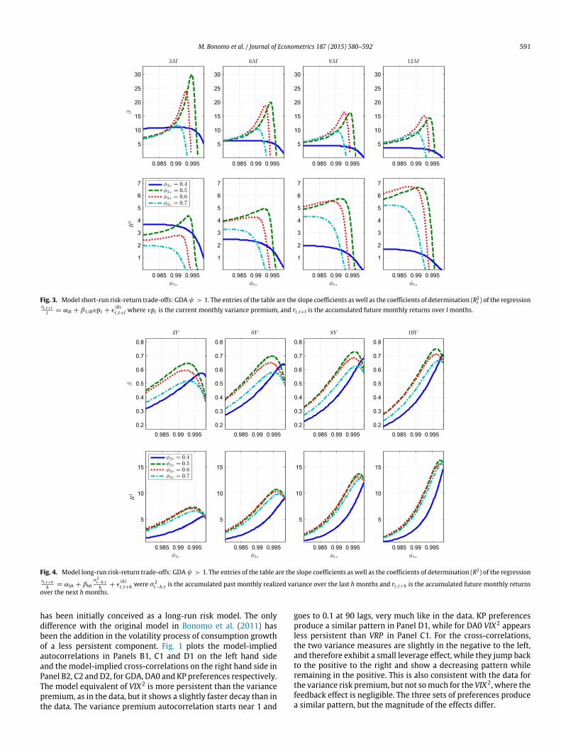
Fig. 3 reports the variations of the regression coefficients andthe R2 for the various horizons aswe vary bothφ1z andφ2z . The pat-terns are quite surprising. For both statistics there is abell patternwith a maximum on either side of our benchmark value of 0.995for φ1z , depending on the value of φ2z . The only exception is themonotonically decreasing pattern for the 0.4 value of φ2z . There-fore, despite the fact that the empirical patterns are reproduced,the values of the statistics are quite sensitive to the values of thevolatility persistence parameters. Therefore, it appears quite chal-lenging to capture with precision these key parameters by usualmoment-based estimation procedures.

In Table 7,we report the regression coefficients and the R2 of thelong-run risk-return trade-off regressions, that is the regressionsof cumulative returns for a number of months (from 12 to 120)over the cumulative realized volatility for the same number ofmonths. Again the pattern in the data, increasing R2 as the horizonlengthens, is well captured by the GDA model. Therefore weprovide a model for rationalizing the empirical fact put forwardby Bandi and Perron (2008). The risk-return trade-off is hard to findin the short-run but comes out clearly in the long run. BothDA0 andKP produce similar patterns but the R2 values are much smaller.

Fig. 4 reports the variations of the regression coefficients andthe R2 for the various horizons as we vary both φ1z and φ2z .Patterns are monotonically increasing with persistence for boththe coefficients and the R2 up to a high value of φ1z , close to 0.995.From that point on, they start to decrease.

5.2.4. High-frequency dynamicsWe have left for the end perhaps the most challenging stylized

facts, the autocorrelations of the daily measures of the risk-neutral expectation of the integrated variance and of the variancepremium, as well as their daily cross-correlations with returns.This is the risk-return trade-off at the high-frequency level. Eventhough we write the model at a daily frequency, the model

M. Bonomo et al. / Journal of Econometrics 187 (2015) 580–592 591

Fig. 3. Model short-run risk-return trade-offs: GDAψ > 1. The entries of the table are the slope coefficients aswell as the coefficients of determination (R2l ) of the regression

rt,t+ll = α0l + β1,0lvpt + ϵ

(0)t,t+l where vpt is the current monthly variance premium, and rt,t+l is the accumulated future monthly returns over l months.

Fig. 4. Model long-run risk-return trade-offs: GDAψ > 1. The entries of the table are the slope coefficients as well as the coefficients of determination (R2) of the regressionrt,t+h

h = αhh + βhhσ 2t−h,th + ϵ

(h)t,t+h were σ 2

t−h,t is the accumulated past monthly realized variance over the last hmonths and rt,t+h is the accumulated future monthly returnsover the next h months.

has been initially conceived as a long-run risk model. The onlydifference with the original model in Bonomo et al. (2011) hasbeen the addition in the volatility process of consumption growthof a less persistent component. Fig. 1 plots the model-impliedautocorrelations in Panels B1, C1 and D1 on the left hand sideand themodel-implied cross-correlations on the right hand side inPanel B2, C2 and D2, for GDA, DA0 and KP preferences respectively.The model equivalent of VIX2 is more persistent than the variancepremium, as in the data, but it shows a slightly faster decay than inthe data. The variance premium autocorrelation starts near 1 and

goes to 0.1 at 90 lags, very much like in the data. KP preferencesproduce a similar pattern in Panel D1, while for DA0 VIX2 appearsless persistent than VRP in Panel C1. For the cross-correlations,the two variance measures are slightly in the negative to the left,and therefore exhibit a small leverage effect, while they jump backto the positive to the right and show a decreasing pattern whileremaining in the positive. This is also consistent with the data forthe variance risk premium, but not somuch for the VIX2, where thefeedback effect is negligible. The three sets of preferences producea similar pattern, but the magnitude of the effects differ.

592 M. Bonomo et al. / Journal of Econometrics 187 (2015) 580–592

5.2.5. Robustness to the value of the elasticity of intertemporalsubstitution

The value of the elasticity of intertemporal substitution ψ is amatter of debate. Bansal and Yaron (2004) argue for a value largerthan 1 for this parameter since it is critical for reproducing theasset pricing stylized facts. Given this debate over the value of theelasticity of substitution ψ , we set it at 0.75. We maintain for theother parameters the same values as in the benchmark model. Inthe online appendix we include the graphs corresponding to thesensitivity analysis with respect to the values of φ1z and φ2z for theasset pricingmoments, the variance premiummoments, the short-run risk-return trade-off and the long-run risk-return trade-off inFigs. 2 to 5 respectively. These figures should be compared to thecorresponding figures with our benchmark GDA specification withψ greater than one (equal to 1.5). A careful comparison shows thatthe value of ψ does not change at all the patterns for the variousstatistics, while it may affect marginally their magnitudes.

6. Conclusion

We have assessed the ability of a long-run risk equilib-riumwhere preferences display generalized disappointment aver-sion (Routledge and Zin, 2010) to capture various stylized facts,high-frequency, short-run and long-run, about the risk-returntrade-off in addition to the usual asset pricing moments and thereturn predictability by the dividend-price ratio. We have there-fore written the model developed in Bonomo et al. (2011) at thedaily frequency andderived closed-form formulas for all these styl-ized facts. For the dynamics of the consumption growth processwehave maintained a random walk in consumption with a stochasticvolatility that includes twomean-reverting components, onemuchmore persistent than the other. Moreover we maintain the samecalibration as in Bonomo et al. (2011) for the preference parame-ters.

Overall, our results are quite supportive of the model. Wemanage to match rather well most empirical facts, moments aswell as predictability patterns, for both asset pricing and risk-return trade-off statistics at all horizons. We observe that puredisappointment aversion is not enough to capturemost risk-returntrade-off statistics, contrary towhatwe concluded in Bonomo et al.(2011) for asset pricing moments and return predictability by theprice-dividend ratio. Therefore, both disappointment aversion andshort-run risk aversion play a role in explaining risk-return trade-off stylized facts.

A remaining challenge concerns the variance of the variance riskpremium, which is too low in our model. We could of course find acalibration that does better in that dimension but it will be at theexpense of other stylized facts. We will leave this difficult task forfuture work.

Appendix A. Supplementary data

Supplementary material related to this article can be foundonline at http://dx.doi.org/10.1016/j.jeconom.2015.02.040.

References

Alizadeh, S., Brandt,M.W., Diebold, F.X., 2002. Range-based estimation of stochasticvolatility models. J. Finance 57 (3), 1047–1091.

Andersen, T., Bollerslev, T., Meddahi, N., 2005. Correcting the errors: Volatilityforecast evaluation using high-frequency data and realized volatilities.Econometrica 73, 279–296.

Bandi, F., Perron, B., 2008. Long-run risk-return trade-offs. J. Econometrics 143,349–374.

Bansal, R., Kiku, D., Yaron, A., 2012. An empirical evaluation of the long-run risksmodel for asset prices. Crit. Finance Rev. 1 (1), 183–221.

Bansal, R., Yaron, A., 2004. Risks for the long run: A potential resolution of assetpricing puzzles. J. Finance 59 (4), 1481–1509.

Barndorff-Nielsen, O., Shephard, N., 2001. Non-gaussian ornstein-uhlenbeck-basedmodels and some of their uses in financial economics. J. R. Stat. Soc. B 63,167–207.

Black, F., Cox, J.C., 1976. Valuing corporate securities: Some effects of bondindenture provisions. J. Finance 31 (2), 351–367.

Bollerslev, T., Litvinova, J., Tauchen, G., 2006. Leverage and volatility feedbackeffects in high-frequency data. J. Financ. Econometrics 4 (3), 353–384.

Bollerslev, T., Sizova, N., Tauchen, G., 2012. Volatility in equilibrium: Asymmetriesand dynamic dependencies. Rev. Finance 16, 31–80.

Bollerslev, T., Tauchen, G., Zhou, H., 2009. Expected stock returns and variance riskpremia. Rev. Financial Studies 22 (11), 4463–4492.

Bollerslev, T., Zhou, H., 2005. Volatility puzzles: A unified framework for gaugingreturn-volatility regressions. J. Econometrics 131, 123–150.

Bonomo, M., Garcia, R., 1994. Can a well-fitted equilibrium asset pricing modelproduce mean reversion. J. Appl. Econometrics 9, 19–29.

Bonomo, M., Garcia, R., 1996. Consumption and equilibrium asset pricing: Anempirical assessment. J. Empirical Finance 3, 239–265.

Bonomo, M., Garcia, R., Meddahi, N., Tédongap, R., 2011. Generalized disappoint-ment aversion, long-run volatility risk and aggregate asset prices. Rev. FinancialStud. 24 (1), 82–122.

Calvet, L.E., Fisher, A.J., 2007. Multifrequency news and stock returns. J. FinancialEcon. 86 (1), 178–212.

Cecchetti, S., Lam, P.-S., Mark, N., 1990. Mean reversion in equilibrium asset prices.Amer. Econ. Rev. 80, 398–418.

Chernov, M., Gallant, R., Ghysels, E., Tauchen, G., 2003. Alternative models for stockprice dynamics. J. Econometrics 116, 225–257.

Corsi, F., 2009. A simple long-memory model of realized volatility. J. FinancialEconometrics 7, 174–196.

Drechsler, I., 2013. Uncertainty, time-varying fear, and asset prices. J. Finance 68(5), 1843–1889.

Drechsler, I., Yaron, A., 2011. What’s vol got to do with it? Rev. Financial Stud. 24(1), 1–45.

Epstein, L.G., Zin, S.E., 1989. Substitution, risk aversion, and the temporal behaviorof consumption and asset returns: A theoretical framework. Econometrica 57(4), 937–969.

Epstein, L.G., Zin, S.E., 1991. Substitution, risk aversion, and the temporal behaviorof consumption and asset returns: An empirical analysis. J. Political Economy99 (2), 263–286.

Hansen, L.P., Heaton, J.C., Li, N., 2008. Consumption strikes back? Measuring long-run risk. J. Polit. Econ. 116 (2), 260–302.

Kreps, D.M., Porteus, E.L., 1978. Temporal resolution of uncertainty and dynamicchoice theory. Econometrica 46 (1), 185–200.

Lettau, M., Ludvigson, S., 2010. Measuring and modeling variation int he risk-return trade-off. In: At-Sahalia, Yacine, Peter Hansen, Lars (Eds.), Handbook ofFinancial Econometrics, Vol. 1, pp. 617–690.

Meddahi, N., 2001. An Eigenfunction Approach for Volatility Modeling. CIRANOWorking paper, 2001s-70.

Meddahi, N., 2002. A theoretical comparison between integrated and realizedvolatility. J. Appl. Econometrics 17, 479–508.

Newey, W., West, K., 1987. A simple positive semi-definite, heteroskedasticity andautocorrelation consistent covariance matrix. Econometrica 55, 703–708.

Rossi, A., Timmermann, A., 2010. What is the Shape of the Risk-Return Relation?Working paper, University of California, San Diego.

Routledge, B.R., Zin, S.E., 2010. Generalized disappointment aversion and assetprices. J. Finance 65 (4), 1303–1332.

Schreindorfer, D., 2014. Tails, Fears, and Equilibrium Option Prices. Working paper.