the locomotive assignment problem with distributed power
TRANSCRIPT

Submitted to Transportation Sciencemanuscript (Please, provide the manuscript number!)
Authors are encouraged to submit new papers to INFORMS journals by means ofa style file template, which includes the journal title. However, use of a templatedoes not certify that the paper has been accepted for publication in the named jour-nal. INFORMS journal templates are for the exclusive purpose of submitting to anINFORMS journal and should not be used to distribute the papers in print or onlineor to submit the papers to another publication.
The Locomotive Assignment Problem withDistributed Power at the Canadian National
Railway Company
Camilo Ortiz-AstorquizaDepartamento de Matematicas, Pontificia Universidad Javeriana, Bogota, Colombia, [email protected],
Jean-Francois CordeauHEC Montreal, Canada, [email protected]
Emma FrejingerDepartment of Computer Science and Operational Research, Universite de Montreal, Canada,
Some of the most important optimization problems faced by railway operators arise from the management
of their locomotive fleet. In this paper, we study a general version of the locomotive assignment problem
encountered at the tactical level by one of the largest railroads in North America: the Canadian National
Railway Company (CN). We present a modeling framework with two integer linear programming formulations
and contribute to the state of the art by allowing to decide each train’s operating mode (distributed power
or not) over the whole (weekly) planning horizon without partitioning it into smaller time windows. Given
the difficulty to solve the problem, one of the formulations is enhanced through various refinements such as
constraint relaxations, preprocessing and fixed cost approximations. We thus achieve a significant reduction
in the required computational time to solve instances of realistic size. We also present two versions of a
Benders decomposition-based algorithm to obtain feasible solutions. On average, it allows to reduce the
associated computational time by two hours. Results from an extensive computational study and a case
study with data provided by CN confirm the potential benefits of the model and solution approach.
Key words : Locomotive planning, Network optimization, Railway transportation, Integer programming
1

Ortiz-Astorquiza, Frejinger and Cordeau: The Locomotive Assignment Problem with Distributed Power2 Article submitted to Transportation Science; manuscript no. (Please, provide the manuscript number!)
1. Introduction
Locomotive planning plays a crucial role in the overall performance of railway companies.
The high cost of locomotives and the large number of them required to satisfy train sched-
ules make of the locomotive fleet one of their most valuable assets, generally representing
an investment in the order of billions of dollars. Therefore, optimization tools that help in
the locomotive planning process are potentially highly valuable. Although previous stud-
ies have shown significant potential savings, many railway companies still rely on human
experience to solve the complex decision-making problems related to locomotive planning.
Moreover, proper management can have significant social and environmental impacts. For
example, the railway industry represents one of the most important means of transporta-
tion in North America. In Canada only, over 900,000 tons of freight were transported on a
daily basis in 2017 (RAC 2018). In this paper we focus on a tactical locomotive planning
problem faced by one of the largest railway companies in North America, the Canadian
National Railway Company (CN).
The Operations Research (OR) literature on locomotive fleet management distinguishes
two main problem types that match the decision process of most railways, namely, a tactical
and an operational optimization problem. The need to resort to a sequential planning
approach is a consequence of both the complexity of the problems and the types of decisions
to be made. At the tactical stage, it has been referred to as the Locomotive Assignment
Problem (LAP) (Vaidyanathan et al. 2008) whereas at the operational level it is usually
known as the Locomotive Routing Problem (LRP) (Vaidyanathan, Ahuja, and Orlin 2008).
In brief, the LAP consists of determining the number and types of locomotives assigned to
each train of a given schedule so that power requirements and flow balance of locomotives
at stations are met while minimizing an objective function. The typical train schedule is
a weekly plan to be repeated over a three or four-month period. The goal in the LAP is
to obtain a guideline on how to assign locomotive types to trains and reposition them in
the network so that the plan is repeated every week. Then, the LRP is solved weekly to
determine the actual sequence of trains to be operated by each specific locomotive while
honoring other constraints and minimizing the cost.

Ortiz-Astorquiza, Frejinger and Cordeau: The Locomotive Assignment Problem with Distributed PowerArticle submitted to Transportation Science; manuscript no. (Please, provide the manuscript number!) 3
In railway transportation, especially for freight in North America, typically there is more
than one locomotive assigned to operate each train either because the demand for horse
power (HP) cannot be satisfied otherwise or because operating main-line (ML) trains that
are usually long and heavy on long distances or specific corridors with difficult geographic
conditions require reliable consists. A consist is defined as a group of locomotives traveling
together. More importantly, in recent years, CN and many other railway operators have
started moving from the conventional mode where all the active locomotives travel together
at the head of the train to distributed power (DP), where locomotives can be interspersed
throughout the length of the train. DP is a relatively recent technology (Deveau 2011)
which has yielded several patents in the last two decades. However, it also brings an extra
level of complexity to the planning problem. On the one hand, DP reduces the in-train
forces permitting an increase in the length and weight of the train. It also reduces fuel
consumption, wear on various components and the possibility of derailment. On the other
hand, setting up and separating the locomotives that travel on DP mode is more time
consuming and not all locomotives possess the right equipment to be used in this mode.
Thus, in this article, we study a general version of a tactical LAP denoted LAP-DP. We
continue this section with an overview of related work followed by a statement of our
contributions.
1.1. Literature Review
Several articles in the broader context of locomotive scheduling have been published dating
back to the mid 1970’s. Here we mention those that we consider the most relevant ones
for this paper mainly based on the level of planning but we refer the reader to the survey
papers of Cordeau, Toth, and Vigo (1998) and of Piu and Speranza (2014) for a more
complete review of the literature. We note that the problem names and their definitions
may vary in related articles, not necessarily following the classification discussed here.
One of the first works addressing the LAP with a locomotive fleet composed of different
locomotive types was that of Florian et al. (1976). In this case, consists can be formed
of one or more locomotive types to meet HP requirements. The authors proposed a mul-
ticommodity network flow-based model and a Benders decomposition algorithm to solve

Ortiz-Astorquiza, Frejinger and Cordeau: The Locomotive Assignment Problem with Distributed Power4 Article submitted to Transportation Science; manuscript no. (Please, provide the manuscript number!)
the problem. Their model was later generalized by Ziarati et al. (1997) to include other
operational constraints in what they denoted as an LAP at the operational strategic level
requiring no repetitiveness of the solution. Ziarati et al. (1997) proposed a solution method
for full size instances on CN data from 1995 (approx. 2,000 trains per week and 1,200
locomotives) based on dividing the time horizon into a set of rolling and overlapping 1-day
time windows. Every time slice is optimized using a branch-and-bound procedure in which
the Linear Programing (LP) relaxations are solved with a Dantzig-Wolfe decomposition.
The authors also considered maintenance constraints falling into the category of what we
denote as the LRP. In a subsequent paper, Ziarati et al. (1999) presented an improved
solution methodology denoted branch-first, cut-second which significantly reduces the LP
relaxation gap and the overall computing time.
Cordeau, Soumis, and Desrosiers (2000, 2001) presented exact algorithms based on Ben-
ders decomposition to handle the simultaneous assignment of locomotives and cars of
passenger transportation for Via Rail Canada. Ahuja et al. (2005) and Vaidyanathan et al.
(2008) proposed ILP formulations for a tactical version of the LAP considering several
realistic characteristics in collaboration with CSX Transportation. Their formulations are
based on a space-time network representation and can be described under the umbrella of
multicommodity network design problems with integer flows. Ahuja et al. (2005) proved
that the LAP is an NP-hard problem which in turn implies that the LAP-DP also belongs
to this class of problems. The authors also present heuristic methods to solve the mod-
els mainly by removing fixed-charge variables and solving the 1-day version repeatedly
over the full week. Their full size instances contain approximately 3,300 trains and 3,300
locomotives among five locomotive types.
Vaidyanathan et al. (2008) included additional operational constraints and proposed an
improved ILP formulation based on assigning only predefined consists. This idea followed
from the important observation that since an integral number of locomotives must be
assigned, it is very unlikely that there is a consist satisfying exactly the train HP (Ziarati
et al. 1999). In reality, the function of HP over the set of consists is not continuous but
a stepwise function. More importantly, these steps are typically of a few hundreds of HP
which in turn implies a significant gap between the LP relaxation and the ILP solution.

Ortiz-Astorquiza, Frejinger and Cordeau: The Locomotive Assignment Problem with Distributed PowerArticle submitted to Transportation Science; manuscript no. (Please, provide the manuscript number!) 5
Moreover, several side constraints can be implicitly handled in the predefined consists.
Vaidyanathan et al. (2008) discuss the benefits of having a pure consist-based formulation
for the LAP where both active and non-active locomotives travel in the network as consists.
Later, Piu, Kumar, and Speranza (2015) proposed an optimization model to define the
initial set of consists and Jaumard and Tian (2016) proposed a column generation approach
for a similar variant of the LAP.
More recently, Powell et al. (2014) and Bouzaiene-Ayari et al. (2016) presented an
approach based on Approximate Dynamic Programming (ADP) to solve locomotive
scheduling problems for Norfolk Southern. The authors proposed three optimization mod-
els distinguished mainly by the level of detail that define the set of locomotives which is
tightly related with the level of planning. They refer to this family of models as PLASMA
(Princeton Locomotive and Shop MAnagement system). First, they consider a strategic
variant denoted as single commodity formulation (PLASMA/SC) where all locomotives
are assumed to be of the same type. Then, they consider a multicommodity formulation
with four locomotive types (PLASMA/MC) and finally a multi-attribute version in which
each locomotive is identified individually (PLASMA/MA). Note that the PLAMA/MC
and PLASMA/MA versions are similar to what we denote the LAP and LRP, respectively.
One of the important contributions of Bouzaiene-Ayari et al. (2016) was to include and
efficiently handle several sources of uncertainty, especially those relating to time delays.
However, as the authors point out, ADP seems to be well suited to handle high levels of
detail, including uncertainty, but is less skilled at managing a global vision of flows around
the network over time. This means that ADP is possibly not the best approach to deal
with repeatable solutions, i.e., matching ending with beginning inventories, which is our
focus.
1.2. Contributions
To the best of our knowledge, deciding of the operating mode (DP or conventional) has
not been included in the optimization models proposed in the literature nor any benefit
(e.g., reduction in the HP required) that depends on the type of consist. Also, we note that
there is no solution methodology of a general and realistic version of an LAP in which one

Ortiz-Astorquiza, Frejinger and Cordeau: The Locomotive Assignment Problem with Distributed Power6 Article submitted to Transportation Science; manuscript no. (Please, provide the manuscript number!)
considers repetitiveness in the solution without partitioning the train schedule into smaller
time windows. This cyclic behavior is an important modeling aspect when following a
sequential planning approach to facilitate the implementation of the subsequent problem
solution. Furthermore, depending on the train schedule, trains may operate only a few
days per week which can yield suboptimal solutions when solving a daily problem. Thus,
the main contributions of this article are the following.
– We introduce a general version of an LAP denoted as LAP-DP in which the mode
of operation of the trains is part of the decision process. Under this umbrella we consider
the benefits in the HP required depending on consist configuration and we show how it
greatly impacts the objective function value. Additionally, we incorporate other real-life
considerations in the model such as repositioning of inactive locomotives at intermediate
stations and consist busting which are explained in detail in the following sections.
– We present two Integer Linear Programming (ILP) formulations to model the LAP-
DP and we develop various enhancements on one of them to improve the computational
performance when solved with a general-purpose solver. Among other ideas, we propose
constraint relaxations, approximation of fixed costs and criteria to select predefined con-
sists available to be assigned. With the enhanced formulation we obtain good solutions,
compared to actual operations, for real-size instances of the problem within a time limit of
6 hours. Without these refinements and proper implementation of the modeling framework
it is not possible to even obtain feasible solutions within this computing time limit.
– We also develop two versions of an algorithm based on Benders decomposition (Ben-
ders 1962) to obtain feasible solutions in reasonable time and test different variants of
these algorithms to assess their performance. On average, there is a time improvement of
almost two hours to find the first feasible solution in comparison with the enhanced for-
mulation for the full-size instances. Moreover, the results indicate that the Benders-based
algorithms are less dependent on the number of threads used in the experiments.
– We present results and insights from a case study based on real data and guidance
provided by CN for ML freight trains as well as local and yard services requiring planned
locomotive power. All the solutions obtained with the model indicate significant potential
savings in comparison with the actual operations.

Ortiz-Astorquiza, Frejinger and Cordeau: The Locomotive Assignment Problem with Distributed PowerArticle submitted to Transportation Science; manuscript no. (Please, provide the manuscript number!) 7
– We perform an extensive computational study to assess the performance of the for-
mulations on realistic instances. Through a sensitivity analysis on various parameters of
the models, we assess the characteristics of the solutions as well as the performance of
the algorithms. The results show that there is an important impact on both solutions and
algorithmic performance when emphasizing certain parameters of the objective function
and some constraints.
1.3. Paper Structure
The remainder of the paper is organized as follows. In Section 2 we describe the LAP-DP
in detail and in Section 3 we present the modeling framework along with two ILP formula-
tions. In Section 4 we describe the algorithmic refinements on one of the formulations and
two algorithms based on Benders decomposition for the LAP-DP. In Section 5 we present
the computational experiments and the case study and conclusions follow in Section 6.
2. Problem Description
At the tactical level, the goal is to obtain a cyclic solution that provides a guideline for the
subsequent levels of planning. Thus, it becomes unnecessary and rather counterproductive
to determine the routes of individual locomotives at this stage because their operational
conditions and initial positions in the network will vary from week to week. In addition,
the train schedule may suffer small changes every week and, more importantly, there are
decisions associated with individual locomotives that would be difficult or impossible to
comply with when planning three months in advance. Instead, the problem is modeled by
aggregating locomotives into significant types, i.e., assuming that locomotives with similar
specifications and costs are actually indistinguishable. In this context, it is important to
emphasize that the LAP can only be implemented in practice jointly with an LRP solution.
In particular, the LAP-DP consists of determining the optimal assignment of locomotive
types to trains and the choice of operating mode while satisfying power requirements and
flow balance for a given 7-day train schedule. The force required to pull a train is often
expressed in terms of HP which can be met by selecting a set of locomotives, possibly of
different types. Hence, the main output of the LAP-DP is an assignment of consists to
trains.

Ortiz-Astorquiza, Frejinger and Cordeau: The Locomotive Assignment Problem with Distributed Power8 Article submitted to Transportation Science; manuscript no. (Please, provide the manuscript number!)
2.1. Problem Data
The input of the LAP-DP mainly consists of a weekly train schedule with the corresponding
HP demand values and a set of available locomotives partitioned into types. Let K be a
set of locomotive types and AT the set of train legs indexed by l ∈AT .
Trains legs: Each train leg l ∈AT is defined by a type, origin and destination stations, a
length, a tonnage tl, times of departure and arrival, and a parameter βl called Horse Power
to Tonnage (HPT). The train type determines whether a train operates in the mainline
network, which typically implies heavy, long distance trains, or if it is a local or yard
service. The HPT is based on geographical and operational conditions and it allows to
approximate how much HP is needed to pull the tonnage of the train.
Locomotives: Associated with each locomotive type k ∈K are the number of available
locomotives fk, the HP hk, the weight of a locomotive wk, a binary parameter dpk indicat-
ing whether it is DP equipped, the number of axles λk and an indicator that determines
whether it generates DC or AC power. Let B and D be the sets of locomotive types that
generate AC and DC power, respectively.
Network: Information on the rail network is assumed to be available such as each train
route Rl, the railroad distance r(i, j) between stations i and j and power change stations,
which are predefined points in the network where some trains may stop for a consist change.
Costs: We consider fuel consumption costs which depend on the locomotive type, the
train and the diesel cost. Also, we consider a track maintenance cost associated with the
usage of the railroad. There is an ownership cost gk that corresponds to the weekly cost
of using a locomotive of type k. Finally, there are crew costs that depend on the duration
of the train as well as the train type.
2.2. Power Requirements
One of the main constraints of any LAP is to assign sufficient locomotives of the right types
so that one ensures the HP required to pull each train. The typical HP approximation
for a given train leg l is done using βltl. However, an important aspect that may yield
significant savings and is not being considered using this approximation is that the HPT
changes when a train is operated under DP or when the assigned consist is formed of AC
locomotives only. Therefore, a more precise approximation of the HP required is

Ortiz-Astorquiza, Frejinger and Cordeau: The Locomotive Assignment Problem with Distributed PowerArticle submitted to Transportation Science; manuscript no. (Please, provide the manuscript number!) 9
HPl =
βltl if conventional mode
βAl tl if conventional mode and all AC locomotives
(βl− θl)tl if DP mode
(βAl − θl)tl if DP mode and all AC locomotives,
(1)
where βAl and θl model the values of HPT if only AC locomotives are assigned and the
discount on HPT for using DP, respectively.
Another aspect to consider is the power change stations where trains may modify con-
sists. These are well-defined stations in the schedule since it is known where the HPT
varies considerably from one part of the route to the next. One way to include this feature
is by splitting the original train by modifying the origin-destination (OD) into the corre-
sponding parts at power change stations as if they were separate trains in a preprocessing
stage.
2.3. Consist Busting and Train-to-Train Connections
Consist busting is an important decision in locomotive scheduling which plays a major role
in the objective function of existing models, especially for those at the operational level.
We say that a consist is busted if, after arriving at its destination station, the locomotives
are separated and become available individually. Otherwise, when the arriving consist is
assigned without changes to a departing train, we refer to it as a train-to-train connection.
In Section 5.2 we describe in detail how we handle train-to-train connections.
2.4. Flow Balance and Power Availability
An important aspect in locomotive planning is ensuring that there are sufficient loco-
motives of each desired type at each station to satisfy the train schedule. However, the
network is usually unbalanced because some stations require more HP than they receive
through the arriving trains or vice-versa. Stations are called sources when the total HP of
departing trains exceeds that of arriving trains and sinks in the opposite situation. There-
fore, locomotives must be repositioned by other means than as active power on scheduled
trains. This can be done in two ways: (i) deadheading (DH), which indicates that locomo-
tives travel using the scheduled trains but are not pulling, and (ii) light traveling, which
consists of sending groups of locomotives where only the leading one is active and they do

Ortiz-Astorquiza, Frejinger and Cordeau: The Locomotive Assignment Problem with Distributed Power10 Article submitted to Transportation Science; manuscript no. (Please, provide the manuscript number!)
not have additional railcars attached. Note that DH is less costly but in many cases the
only or most rapid way of repositioning locomotives is through light traveling.
An additional feature included in the LAP-DP, that to the best of our knowledge has not
been addressed before, is to allow extra DH. What we denote as “extra” DH is common in
practice and is formed of two parts. First, when there is an active train-to-train connection
the non-active locomotives are allowed to stop or be added at the connecting station.
Second, DH of locomotives that occurs between pairs of stations other than the origin
and destination pair of each scheduled train, i.e., intermediate stations in the train route.
Allowing DH locomotives to be dropped off and picked up in the middle of the train route
at predefined stations has a significant impact in the solution and computing time.
2.5. Additional Constraints
Several side constraints and preferences are considered in the LAP-DP to better capture
the requirements that arise in practice. For example, limiting the number of (active) loco-
motives and the number of active axles per train (al) as well as avoiding mixes of AC with
DC locomotives. Some of these requirements are desirable but not mandatory. We can
also impose that certain trains operate under DP or conventional mode depending on the
length and weight of the train and we promote certain characteristics in the solution by
means of weights in the objective function. Other common features in locomotive planning
such as the use of foreign power (leasing locomotives from other railways), train delays
and maintenance constraints are treated at the operational level.
3. Modeling Framework
We model the LAP-DP via a space-time network that represents the physical railroad
and the train schedule simultaneously. Time units are in minutes and each locomotive
type is considered a commodity to be routed on the network. Let G= (N,A) be a graph
with N the set of nodes and A the set of arcs. Each node i ∈N is associated with three
attributes, namely, station number, time and type, whereas each arc a ∈ A represents
an activity such as a train leg, a waiting period, or repositioning of locomotives, among
others. As in a network flow problem (Ahuja, Magnanti, and Orlin 1993), the flow of a
particular commodity on an arc represents the assignment of this locomotive type to the

Ortiz-Astorquiza, Frejinger and Cordeau: The Locomotive Assignment Problem with Distributed PowerArticle submitted to Transportation Science; manuscript no. (Please, provide the manuscript number!) 11
corresponding activity. We note that most of the notation used throughout this article is
inherited from airline planning problems and from previous work on the LAP.Note that
we refer indistinctly to a train arc and a train leg. Tables 1 and 2 summarize the main
notation for parameters and sets used throughout the paper.
Table 1 Summary of main parameters
hk, λk, wk Horsepower, number of axles and weight of locomotives of type k
dpk Binary parameter indicating if locomotives of type k are DP equipped
fk Number of available locomotives of type k
tl Tonnage of train l ∈AT
βl, βAl Standard and AC-only HPT for train l ∈AT
mA,mT ,mD,mDH Maximum number of locomotives (active, total, DP, DH) per train
r(i, j) Railroad distance between stations i and j
gk Weekly ownership cost for a locomotive of type k
ckl Per unit cost of assigning an active locomotive of type k to train l
dkl Per unit cost of assigning a non-active locomotive of type k on arc l
θl Discount on the train HPT for operating on DP
al Maximum number of active axles for train l ∈AT
ρck Number of locomotives of type k in consist c
Table 2 Summary of sets
K Set of locomotive types or commodities
N , A Sets of nodes and arcs in the space-time network
NA, ND Sets of arrival and departure nodes
NG =NI ∪NR ∪NE ∪NDP Set of ground nodes (initial, grd-arr, grd-dept and DP)
AT Set of train arcs
AG, ADP and AL Sets of inter-ground, DP and light-travel arcs
AC =AR ∪AE ∪AQ Sets of arrival-ground, ground-departure, and train-to-train arcs
ADH Set of extra deadheading arcs
I[i], O[i] Sets of inbound and outbound arcs for each i∈NS Set of arcs that cross the checkpoint
B, D Sets of locomotive types that have AC (or DC) power
Rl Set of stations in the route followed by train l
E(l, i, j)⊆ADH Extra DH arcs available between stations i and j in Rl
Cl Set of predefined feasible consists for train l
CDP Set of predefined consists using DP mode
3.1. Space-time Network
Figure 1 depicts an example of a space-time network with four trains represented with the
bold arcs and four different stations. The dashed and bold-dotted arcs correspond to the

Ortiz-Astorquiza, Frejinger and Cordeau: The Locomotive Assignment Problem with Distributed Power12 Article submitted to Transportation Science; manuscript no. (Please, provide the manuscript number!)
DP node
grd-dept node grd-arrival node
departure node arrival node
initial node
Station 1
Station 2
Station 3
Station 4
Train 1
Train 2
Train 3 Train 4
tr-to-tr
tr-to-tr
Extra DH arc
Figure 1 Example of space-time network on four trains and four stations
cyclic behavior of the solution, light travel and extra DH arcs, respectively. We also show
examples of train-to-train arcs in the figure but we omit the representation of all extra DH
arcs to simplify the diagram.
The set of nodes is partitioned into arrival (NA), departure (ND) and ground nodes
(NG). A train arc goes from a departure to an arrival node and the corresponding train
information defines the station numbers and times for these nodes. Ground nodes are used
to represent the events of locomotives when they are not assigned to a train, i.e., they
are at a station. The set of ground nodes is further partitioned into ground-arrival NR,
ground-departure NE, ground-initial NI and DP NDP nodes. For each arrival node there
is an arrival-ground node and for each departure node there is a ground-departure node.

Ortiz-Astorquiza, Frejinger and Cordeau: The Locomotive Assignment Problem with Distributed PowerArticle submitted to Transportation Science; manuscript no. (Please, provide the manuscript number!) 13
Each one of them has the same station number as its corresponding arrival or departure
node. Each arrival-ground node has the time as its associated arrival node plus an input
parameter that models the time for consist busting. For ground-departure nodes a value
is subtracted from the departure time to model the time of creating a consist. A similar
procedure is followed to create DP nodes. However, we should note that not every train
will be allowed to operate on DP mode. Finally, we have one initial ground node at time
zero for each station.
In the set of arcs we consider train arcs AT , DP arcs ADP , arrival-ground AR, ground-
departure (AE) and train-to-train (AQ) connection arcs (AC =AR ∪AE ∪AQ). Moreover,
for each station we sort by time the ground nodes and create an inter-ground arc between
each sequential ground node forming the set AG of inter-ground arcs. After sorting the
nodes, the last ground node of each station is connected with the corresponding initial
ground node to model the cyclic behavior of the LAP-DP.
The set of extra DH arcs ADH consists of two types of arcs: first, those that are not
train arcs and outbound a departure node and arrive in an appropriate ground node of an
intermediate station of the train route satisfying the travel time. Second, those that depart
from an appropriate ground node of an intermediate station and finish at the arrival node.
Note that using this construction we do not permit all possible cases of partial DH, only
those that depart from or arrive to the associated origin or destination station of the train.
We also limit the number of extra DH arcs by creating only those to or from intermediate
stations with few in or out scheduled trains since they are more likely to need extra DH.
Finally, when an arc crosses the checkpoint, e.g., the arrival time is greater than the
time horizon limit, we modify its destination and define the time attribute of the node
such that it becomes the extra minutes after the checkpoint that is initially past. The set
S is formed by all the arcs crossing the checkpoint as well as the cycle arcs.
3.2. Generating Light Traveling Arcs
Light travel arcs play a major role in the network representation when solving the LAP-DP.
Including all possibilities of light travel arcs is not desired because the size of the network
would increase considerably. The goal is then to select a suitable subset of light travel

Ortiz-Astorquiza, Frejinger and Cordeau: The Locomotive Assignment Problem with Distributed Power14 Article submitted to Transportation Science; manuscript no. (Please, provide the manuscript number!)
arcs for which we follow a similar approach as that of Ahuja et al. (2005). In particular,
we determine origin and destination stations of light travel arcs and their frequency by
establishing the flow of HP in the network without considering the time component. We
thus solve a minimum cost flow problem (Ahuja, Magnanti, and Orlin 1993) where the
supply or demand of each node is given by an approximation of the total inbound HP
minus the total outbound HP. Nodes with positive supply values represent power sinks
and stations with negative supply values are power sources. We define the objective value
coefficient for arc (i, j) as
eij =
r(i, j) if nOpij ≤ 2
r(i, j)α if nOpij ∈ (2, α)
r(i, j)α2 otherwise,
where α is an input parameter and nOpij is the number of scheduled trains to operate
from station i to station j. With this definition we discourage the flow on arcs in the
space network when there are more than a given number of trains that operate an OD
pair assuming that those locomotives can be deadheaded. This partly accounts for not
saturating OD pairs using light travel arcs. Note that if long distance light travel is not
desirable, as in our case study, arcs with a distance above a threshold value can be removed.
Finally, we create light travel arcs between a pair of stations if the corresponding solution
flow is above a given minimum threshold value. We also have an input parameter to
establish how many light travel arcs are created for such pairs. To avoid the creation of
extra nodes in the space-time network, we generate light travel arcs conveniently using the
current set of ground nodes. In particular, we use ground-arrival nodes as origins without
affecting the representation of the model because it is then when locomotives become
available to be sent elsewhere. In practice, it is possible that the locomotives are not sent
exactly at that time as long as it is ensured that they arrive to their destination at the
required time. Similarly, for destination nodes we choose the first ground node that is
available after the corresponding travel time. At that time it is when the locomotives are
possibly needed and can be made available.

Ortiz-Astorquiza, Frejinger and Cordeau: The Locomotive Assignment Problem with Distributed PowerArticle submitted to Transportation Science; manuscript no. (Please, provide the manuscript number!) 15
3.3. A Consist-and-Locomotive Flow-Based Formulation
A common way of modeling an LAP is through integer flows traveling in the space-time
network that represent the number of locomotives of each type on each arc. Previous works
(e.g., Ahuja et al. 2005) have shown that the performance of this type of formulation is
very poor in terms of computing time. We present a new Locomotive-Based Formulation
(LBF) for the particular case of the LAP-DP in the Online Appendix. However, preliminary
computational experiments confirmed the slow performance of this type of formulation
when solved with a general-purpose solver.
Another approach to model the problem is to consider a predefined set of feasible consists
C and to decide through binary variables whether a consist is assigned to a train or not
(Vaidyanathan et al. 2008). In addition, we must also incorporate the operating mode in
the decision. Let Cl ⊆C be the subset of feasible consists for train leg l, including DP and
conventional consists, and ρck be the number of locomotives of type k in consist c ∈ Cl.
Also, consider the subset CDP of consists that operate on DP and its complement CDP ,
the set of consists on conventional mode. As mentioned before, there are numerous benefits
to using a formulation based on consists instead of locomotive flows. For example, we use
the sets Cl to implicitly take into account the HP requirements for each train and the
benefits of using AC-only or DP mode, equivalently to equation (1). Moreover, several side
constraints that appear in the LBF can be handled in the definition of Cl.
Let xcl be a binary variable taking value 1 if consist c is assigned to arc l ∈AT ∪AC ∪ADP
and 0 otherwise, and let ykl be the number of non-active locomotives of type k assigned to
arc l ∈A. Note that since DP consists have to be busted at arrival stations, we still need
to define the y variables as locomotive flows instead of consists of non-active locomotives.
Therefore, we propose a Consist-and-Locomotive Flow-based formulation (CLF) that is
more flexible than a pure consist-based approach in dealing with the repositioning of
locomotives and therefore likely to benefit more from extra DH arcs. Also, let zl = 1 if arc
l ∈AC ∪AL is used and 0 otherwise. Finally, ul are variables to control a soft constraint
that determines the total number of active axles per train.
We denote by ckl the operational cost of assigning an active locomotive of type k to
train l, which is a function of the track maintenance and fuel consumption costs. The

Ortiz-Astorquiza, Frejinger and Cordeau: The Locomotive Assignment Problem with Distributed Power16 Article submitted to Transportation Science; manuscript no. (Please, provide the manuscript number!)
costs dkl vary depending on the arc l, e.g., if l ∈ AT ∪ ADH , dkl corresponds to the cost
of deadheading a locomotive of type k using arc l whereas if l ∈ AL, dkl represents the
unit cost of light traveling a locomotive of type k on arc l. Fixed costs p and bl represent
the cost of activating an arc in the network, which in this case model the fixed costs of
busting and light travel, respectively. In the case of light travel arcs it corresponds to the
associated crew and fuel costs that depend on l. The fixed cost p of busting a consist as
well as the penalties and preferences are more subjective and depend on how much weight
the user wants to place on certain characteristics of the solution. Then, let x be the vector
of decision variables, the total cost TotCLF (x) can be written as
TotCLF(x) =∑k∈K
∑l∈AT
ckl∑c∈Cl
ρckxcl +∑k∈K
∑l∈AC∪ADP
dkl (ykl +∑c∈Cl
ρckxcl ) +
∑k∈K
∑l∈AT∪ADH∪AG∪AL
dkl ykl
+∑k∈K
∑l∈S
gk(ykl +∑c∈Cl
ρckxcl ) +
∑l∈AR
pzl +∑l∈AL
blzl +∑l∈AT
ul +PCLF (x),
where PCLF (x) is a function associated with weights for penalties and preferences of solu-
tion features such as mix AC-DC consists and DP, among others. Then, given the sets I[i]
and O[i] of inbound and outbound arcs of node i ∈N , respectively, and E(l, i, j) the set
of extra DH arcs between stations i and j associated with train route Rl, the CLF can be
stated as
minimize TotCLF(x) (2)
subject to∑c∈Cl
xcl = 1 ∀ l ∈AT (3)∑
l∈I[i]
xcl =
∑l∈O[i]
xcl ∀ i∈NA ∪ND, c∈Cl (4a)∑
l∈I[i]
ykl =∑l∈O[i]
ykl ∀ i∈NA ∪ND ∪NI , k ∈K (4b)∑l∈I[i]
(ykl +∑c∈Cl
ρckxcl ) =
∑l∈O[i]
ykl ∀ i∈NR, k ∈K (4c)∑l∈I[i]
ykl =∑l∈O[i]
(ykl +∑c∈Cl
ρckxcl ) ∀ i∈NE ∪NDP , k ∈K (4d)∑
k∈K
∑l∗∈E(l,i,j)
ykl∗ +∑k∈K
∑c∈Cl
ρckxcl ≤mT ∀ l ∈AT , i, j ∈Rl (5)

Ortiz-Astorquiza, Frejinger and Cordeau: The Locomotive Assignment Problem with Distributed PowerArticle submitted to Transportation Science; manuscript no. (Please, provide the manuscript number!) 17∑
k∈K
(ykl +∑c∈Cl
ρckxcl )≤mT zl ∀ l ∈AC (6)∑
k∈K
(ykl +∑c∈Cl
ρckxcl )≤mT
∑c∈Cl∗∩CDP
xcl∗ ∀ l= (i, j)∈ADP , l
∗ ∈AT ∩O[j] (7)
∑k∈K
ykl ≤mT zl ∀ l ∈AL (8)∑l∈O[i]:l∈AQ
zl ≤ 1 ∀ i∈NA (9)
∑l∈I[i]:l∈AQ
zl ≤ 1 ∀ i∈ND (10)
∑k∈K
∑c∈Cl
ρckxcl ≥ 2zl ∀ l= (i, j)∈AQ, j ∈ND (11)
zl ≤ 1−∑
c∈Cl∩CDP
xcl∗ ∀ l ∈AQ ∩O[j], l∗ = (i, j)∈AT (12)
∑c∈Cl∩CDP
xcl ≤ 1−
∑l∗∈AQ∩I[j]
zl∗ ∀ l= (i, j)∈AE (13)
∑l∈I[i]:l/∈AE
(zl +∑
c∈Cl∩CDP
xcl )≤ 1 ∀ i∈ND (14)
zl∗ ≤ 1−∑
c∈Cl∩CDP
xcl ∀ l∗ = (i, j)∈AE, l ∈ADP ∩ I[j] (15)
∑c∈Cl
∑k∈K
λkρckxcl −ul ≤ al ∀l ∈AT (16)∑
l∈S
(ykl +∑c∈Cl
ρckxcl )≤ fk ∀ k ∈K (17)
xcl ∈Z+ ∀ l ∈AT ∪AC ∪ADP , c∈Cl (18)
ul ∈Z+ ∀ l ∈AT (19)
zl ∈ {0,1} ∀l ∈AC ∪AL. (20)
ykl ∈Z+ ∀ l ∈A, k ∈K, (21)
where mT is the maximum number of locomotives allowed on any train. Constraints (3)
ensure that the horsepower requirement for every train is met. Note that depending on the
selection of DP mode or AC-only consists, the HPT of the train may vary, thus affecting the
overall HP required handled with Cl. Equations (4a)–(4d) are flow conservation constraints
and take into account when locomotives become inactive at stations. Constraints (5) limit

Ortiz-Astorquiza, Frejinger and Cordeau: The Locomotive Assignment Problem with Distributed Power18 Article submitted to Transportation Science; manuscript no. (Please, provide the manuscript number!)
the maximum number of locomotives per train. Note that when the set E(l, i, j) = {l} we
are in the particular case of no extra DH at intermediate stations. The sets of constraints
(6)–(8) link the flow variables with the binary variables and limit the maximum number
of locomotives on AC , AL and ADP , respectively. Constraints (9) and (10) establish that
at most one train-to-train connection is allowed at each train arrival or train departure
node while (11) guarantee that a train-to-train connection can only be used for consists of
size greater than one. Constraints (12) consider that when a train operates on DP mode,
a train-to-train connection at the arrival station is not possible. Similarly, constraints (13)
ensure that if a train-to-train connection occurs at a train-departure node, the DP mode
cannot be used on that train and vice-versa. Note that in (13) we do not include the
variable associated with ground-departure arcs, this means that both a ground-departure
and a train-to-train arc could be active which allows to add DH locomotives in a train-
to-train connection. Constraints (14) guarantee that each train either operates on DP or
conventional mode. The set of constraints (15) ensures that if there is a train-to-train
connection, no new active locomotives can be added to the consist. Constraints (16) control
the maximum number of active axles per train and constraints (17) impose the number of
available locomotives by type. In addition, other operational requirements are included by
fixing variables or through the preprocessing of sets Cl.
Note that if we include all possible consists in C, the optimal solution value obtained
with the CLF would be the same as that of the LBF. Moreover, some terms of the LBF can
be transformed into those of the CLF by using a simple transformation of the x variables
and the appropriate use of the sets Cl, B, D and CDP . Also, note that although the xcl
variables model the assigned active consist on a train, they are defined on a larger set
which becomes useful when modeling extra DH through train-to-train connections.
4. Solution Methodology
As mentioned before, we rely on the CLF which significantly reduces the computational
burden in comparison with the LBF. Nevertheless, the difficulty of solving the model
without partitioning the problem into daily subproblems remains very high. Hence, we
now discuss several enhancements to the CLF that exploit the problem definition and its
structure. We also present two Benders-based algorithms to obtain feasible solutions.

Ortiz-Astorquiza, Frejinger and Cordeau: The Locomotive Assignment Problem with Distributed PowerArticle submitted to Transportation Science; manuscript no. (Please, provide the manuscript number!) 19
4.1. Algorithmic Refinements of the CLF Formulation
In addition to the considerations for creating the space-time network we propose several
refinements on the CLF that have an important impact on the overall model performance.
4.1.1. Dominated Consists The idea of a dominated consist takes into account
that the operator uses as few locomotives as possible satisfying the train requirements.
For instance, if we have five locomotive types and consists c1 = (2,0,0,0,0) and c2 =
(3,0,0,0,0), assuming that both are capable of providing the HP required (i.e., c1, c2 ∈Cl),
there is no reason for choosing c2 over c1 for train l ∈AT unless that is the only feasible
consist or possibly by other operational exceptions. For example, in an enforced train-to-
train connection, one of the connecting trains may appear to be overpowered since the
HP required based on tonnage and HPT typically does not match the one of the other
connecting train. However, apart from these types of exceptions there is no reason for
overpowering a train since we may reposition locomotives by DH. This is also an implicit
rule of operations that we can exploit in the modeling process. Another example occurs
when we have c1 = (0,1,1,0,0) and c2 = (0,2,2,0,0). In those cases we say that consist c2
is dominated by c1. In general we have the following definition.
Definition 1. Let l ∈AT and c1 = (c11, . . . , c
1|K|), c
2 = (c21, . . . , c
2|K|)∈Cl with the sets of
indices S1 = {j ∈K : c1j 6= 0} and S2 = {j ∈K : c2
j 6= 0} representing the locomotive types
in the consists. We say that c1 dominates c2 if
a) c1 and c2 are formed by the same locomotive types (S1 = S2) and c1j = c1
i for all
i, j ∈ S1 and c2j = c2
i for all i, j ∈ S2 and
b) c1j < c
2j for all j ∈ S1.
Thus, we can reduce the size of the sets Cl by removing dominated consists when l ∈AT
is not part of a forced train-to-train connection (or possibly other exceptions) without
affecting the optimal solution. More importantly, we can introduce the concept of a consist
type which takes one step further the transition from the LBF to the CLF into a consist-
type assignment. This means that in the set of consists C we can define all possible
variations of a consist type without increasing the number of variables. This facilitates the
search for feasible and better solutions.

Ortiz-Astorquiza, Frejinger and Cordeau: The Locomotive Assignment Problem with Distributed Power20 Article submitted to Transportation Science; manuscript no. (Please, provide the manuscript number!)
4.1.2. Deadheading Constraints As explained in Section 3.1, we select some extra
DH arcs. In particular, we determine which stations are more likely to need repositioning
of locomotives using a threshold value on the number of trains that arrive and depart from
each station. If a station has few trains arriving, we allow extra DH arcs to that station
and similarly with departing trains.
Now, since DH is being minimized in the objective function, and because of locomotive
availability over time in the network, we noticed that in most cases constraints (5) are
not tight. Moreover, since the number of active locomotives is determined in the consist
definition, these constraints are actually limiting the number of DH locomotives, which
could be handled in a post-processing step. For instance, we could inspect the solution
and determine if the number of DH locomotives can exceptionally exceed the limit for a
specific train or if some of those locomotives should be sent in another train or as light
travel. Nevertheless, we do not remove all DH constraints but rewrite them as
∑k∈K
∑l∗∈E(l,o[l],j)
ykl∗ ≤mDH ∀ l ∈AT , j ∈Rl (22)∑k∈K
∑l∗∈E(l,i,d[l])
ykl∗ ≤mDH ∀ l ∈AT , i∈Rl, (23)
where o[l] and d[l] are the origin and destination stations of train l ∈AT and mDH is the
maximum number of DH locomotives allowed on each train. We proceed in a similar way
with constraints (6) and (7) and rewrite them as
∑c∈Cl
xcl ≤ zl ∀ l ∈AC (24)∑
k∈K
ykl ≤mDHzl ∀ l ∈AC (25)
xcl ≤ xc
l∗ ∀c∈Cl ∩CDP , l= (i, j)∈AT , l∗ ∈ADP ∩ I[i] (26)
xcl = 0 ∀c∈Cl ∩CDP , l ∈ADP (27)∑
k∈K
ykl ≤mDH∑
c∈Cl∗∩CDP
xcl∗ ∀ l= (i, j)∈ADP , l
∗ ∈AT ∩O[j]. (28)

Ortiz-Astorquiza, Frejinger and Cordeau: The Locomotive Assignment Problem with Distributed PowerArticle submitted to Transportation Science; manuscript no. (Please, provide the manuscript number!) 21
4.1.3. Approximating Light Travel Fixed Costs In both formulations proposed
there are binary variables that represent the activation of arcs. In particular, the fixed
cost associated with zl for l ∈ AL corresponds to the crew cost plus the fuel cost, both
of which depend on the duration and distance of the light travel train. However, it is
well-known that having fixed-charged variables, i.e., a network design version, makes the
problem harder to solve than the associated pure network flow variant.
Preliminary computational experiments show that when using these costs the solutions
present a large number of active light travel arcs. This behavior is undesirable but can be
explained by the fact that ownership and operational costs represent most of the objective
function value as shown in Section 5. Therefore, the model chooses to open several light
travel arcs if that means using fewer locomotives. One way of partly mitigating this without
including more capacity constraints is to consider a fake penalty cost on light travel arcs.
We therefore propose to substitute fixed costs associated with light travel arcs by adding
an approximate value of crew and fuel costs in the variable costs d. In practice this would
represent paying the approximate crew and fuel costs for each locomotive that is sent in
a light travel train. For our purpose this also serves as a penalty cost to discourage the
usage of light travel trains. However, once we remove these fixed-charge costs it is possible
that the model yields more than one light travel train between a pair of stations, which
could be merged in a post processing step. Yet another way of limiting the total number
of light travel arcs is by adding the constraint
∑l∈AL
zl ≤mli,
where mli is the maximum number of light travel trains allowed in the network.
4.1.4. Removing Variables and Constraints In this case, we remove variables
from the model either by substitution or by fixing them to certain values given the prob-
lem structure or specific operational requirements. Initially, we could replace the binary
variables zl since
zl =∑c∈C
xcl ∀ l ∈AC .

Ortiz-Astorquiza, Frejinger and Cordeau: The Locomotive Assignment Problem with Distributed Power22 Article submitted to Transportation Science; manuscript no. (Please, provide the manuscript number!)
However, preliminary computational experiments showed that the most beneficial substi-
tution occurs when we only consider l ∈AR. Moreover, we add the redundant constraints∑l∈O[i]
∑c∈Cl
xcl = 1 ∀i∈NA. (29)
We also remove variables that were initially defined for all consists in the set of con-
necting arcs. For example, xcl = 0 for l ∈ AC and c ∈ CDP or for l ∈ ADP we set xc
l = 0
for c∈Cl ∩CDP . Another case occurs for the DH variables in outposts trains. An outpost
is a local train that departs from and arrives at the same station. Therefore, we can set
ykl = 0 for all k ∈K if o[l] = d[l] for l ∈AT . Note that we can still allow for partial DH to
intermediate stations and when we approximate costs for light travel arcs we can set zl = 1
for all l ∈AL.
4.2. Benders Decomposition
Benders decomposition is a well-known partitioning method applicable to mixed integer
programs (Benders 1962). It decomposes the original formulation into two simpler ones:
an integer master problem and a linear subproblem. The main idea is to reformulate the
problem by projecting out the set of complicating variables to obtain a formulation with
fewer variables but with a large number of constraints called Benders cuts. Usually only a
small subset of these constraints are active in an optimal solution, a natural approach is
therefore to generate them on the fly. A modern implementation of the algorithm considers
the Benders reformulation within a standard branch-and-cut framework, in which Benders
cuts are separated not only at integer solutions but also at fractional ones at the nodes
of a single enumeration tree. The increased attention that this method has attracted in
the last few years is noteworthy yielding numerous successful implementations in various
fields of OR (e.g., Adulyasak, Cordeau, and Jans 2015, Fischetti, Ljubic, and Sinnl 2017,
Rahmaniani et al. 2017, Ortiz-Astorquiza, Contreras, and Laporte 2019).
Our motivation for applying Benders decomposition to the CLF lies mainly in the prob-
lem structure. Indeed, in the formulation we can distinguish two types of variables: those
that correspond to the activation of arcs and assignment of consists (z and x), and those
that represent the repositioning of non-active locomotives (y). In other words, we can think

Ortiz-Astorquiza, Frejinger and Cordeau: The Locomotive Assignment Problem with Distributed PowerArticle submitted to Transportation Science; manuscript no. (Please, provide the manuscript number!) 23
of the master problem as an assignment generator whose solution is validated with the sub-
problem where we determine through repositioning of locomotives if the given assignment
is feasible and optimal.
Once we fix the x, z and u variables, the formulation becomes a multi-commodity net-
work flow problem on the y variables which are required to be integer. Thus, for fixed
values x, z and u, using the sets of capacity constraints (22)–(28), the CLF reduces to
minimize∑
l∈AC∪ADP
∑k∈K
dkl ykl +
∑l∈AT∪AG∪AL
dkl ykl +
∑k∈K
∑l∈S
gkykl (30)
subject to∑l∈I[i]
ykl =∑l∈O[i]
ykl ∀ i∈NA ∪ND ∪NI , k ∈K (31a)∑l∈O[i]
ykl −∑l∈I[i]
ykl =∑k∈K
∑c∈Cl
ρckxcl ∀ i∈NR, k ∈K (31b)∑
l∈I[i]
ykl −∑l∈O[i]
ykl =∑k∈K
∑c∈Cl
ρckxcl ∀ i∈NE ∪NDP , k ∈K (31c)∑
k∈K
ykl ≤mDH zl ∀ l ∈AE ∪AQ (32)∑k∈K
ykl ≤mT zl ∀ l ∈AL (33)∑k∈K
ykl ≤mDH∑
c∈Cl∗∩CDP
xcl∗ ∀ l= (i, j)∈ADP , l
∗ ∈AT ∩O[j] (34)
∑l∈S
ykl ≤ fk−∑l∈S
∑c∈Cl
xcl ∀ k ∈K (35)∑
k∈K
∑l∗∈E(l,o[l],j)
ykl∗ ≤mDH ∀ l ∈AT , j ∈Rl (36)∑k∈K
∑l∗∈E(l,i,d[l])
ykl∗ ≤mDH ∀ l ∈AT , i∈Rl (37)
ykl ∈Z+ ∀ l ∈A, k ∈K. (38)
However, the decomposition procedure requires finding the values of the dual variables
of constraints (31a)–(37) to generate Benders cuts. We relax the integrality requirement of
constraints (38) to define the primal subproblem (SP) but in general, it does not have the
integrality property. Moreover, the integer version of the SP may be infeasible even when
its LP relaxation is feasible. In this case the generated Benders cut might fail to remove
the infeasible integer programming solution. One way to deal with this would be to use

Ortiz-Astorquiza, Frejinger and Cordeau: The Locomotive Assignment Problem with Distributed Power24 Article submitted to Transportation Science; manuscript no. (Please, provide the manuscript number!)
ad-hoc combinatorial feasibility cuts. However, we present a different approach in the next
section. For the moment, let ∆ be the set of feasible points of the dual subproblem, and
P∆ and R∆ be the sets of extreme points and extreme rays of ∆, respectively. The Benders
reformulation master problem (MP) is
minimize η+∑k∈K
∑l∈AT
ckl∑c∈Cl
ρckxcl +∑k∈K
∑l∈AC∪ADP
dkl∑c∈Cl
ρckxcl +∑k∈K
∑l∈S
gk∑c∈Cl
ρckxcl+∑
l∈AR
pzl +∑l∈AL
blzl +∑l∈AT
ul +PCLF (x) (39)
subject to (3), (4a), (9)− (16), (18)− (20)
0≥∑k∈K
∑i∈NE∪NDP
∑l∈O[i]
∑cinCl
ρckxclπ
ki −
∑i∈NR
∑l∈I[i]
∑c∈Cl
ρckxclπ
ki
−∑
l∈AE∪AQ
(mDHzl−
∑k∈K
∑c∈Cl
ρckxcl
)ωl−
∑l∈AL
mT zlωl−∑
l∈ADP
mDH∑
c∈Cl∗∩CDP
xcl∗ωl−
∑k∈K
(fk−
∑l∈S
∑c∈Cl
xclβk
)−∑l∈AT
(∑j∈Rl
mDHβjl +
∑i∈Rl
mDHβil
)∀ δ ∈R∆ (40)
η≥∑k∈K
∑i∈NE∪NDP
∑l∈O[i]
∑cinCl
ρckxclπ
ki −
∑i∈NR
∑l∈I[i]
∑c∈Cl
ρckxclπ
ki
−∑
l∈AE∪AQ
(mDHzl−
∑k∈K
∑c∈Cl
ρckxcl
)ωl−
∑l∈AL
mT zlωl−∑
l∈ADP
mDH∑
c∈Cl∗∩CDP
xcl∗ωl−
∑k∈K
(fk−
∑l∈S
∑c∈Cl
xclβk
)−∑l∈AT
(∑j∈Rl
mDHβjl +
∑i∈Rl
mDHβil
)∀δ ∈ P∆, (41)
where δ = (π,β,ω) is a vector of dual variables in ∆ and η is an additional decision
variable representing a lower bound on the cost of the subproblem. Constraints (40) and
(41) are the Benders feasibility and optimality cuts, respectively.
4.3. Finding Feasible Solutions
Despite all the model enhancements it remains challenging to find feasible solutions for full-
size instances of the LAP-DP. Therefore, we exploit the Benders decomposition structure
to develop an algorithm that reduces the computing time to find feasible solutions of the

Ortiz-Astorquiza, Frejinger and Cordeau: The Locomotive Assignment Problem with Distributed PowerArticle submitted to Transportation Science; manuscript no. (Please, provide the manuscript number!) 25
CLF. This may have an impact on the branch-and-bound procedure by providing an upper
bound to prune nodes but also serve as an alternative approach for solving the model.
First, note that using a similar flow of argumentation as in Section 4.1.2 we can relax
constraints (32)–(34), (36) and (37) and replace each set of these capacity constraints by
|K| of them, one per locomotive type. We are thus limiting the number of DH locomo-
tives by type and not the total number of them on each arc. The resulting problem is
then decomposable into |K| independent problems. Moreover, in the particular case where
E(l, i, j) = {l} for all l ∈ AT and i = o[l] and j = d[l], the feasibility of the resulting LP
subproblem implies the feasibility of the integer counterpart (see Proposition 1 in Cordeau,
Soumis, and Desrosiers 2000). For the general case in which extra DH is permitted at
intermediate stations, we check the feasibility of the ILP when the solution of the LP is
not integral. In the computational experiments, only in very rare occasions do we have to
validate the feasibility of the ILP. Another approach is to completely ignore the extra DH
capacity constraints so that the resulting LP has the feasibility property and reintroduce
them at a postprocessing stage.
4.3.1. Surrogate Constraints The large number of feasibility cuts is caused by the
lack of information in the restricted MP which no longer has all the constraints. The
restricted MP is in a sense myopic because constraints (17) that limit the number of
available locomotives are not considered. Therefore, each assignment that does not satisfy
the locomotive availability constraints in the SP needs a feasibility cut. This issue can
be partly managed by using surrogate constraints in the restricted MP. In addition to
constraints (29) we propose the following families of valid inequalities:
xcl = 0 ∀ c∈Cl ∩CDP , l ∈AE ∪AQ (42)∑
l∈Γq
∑c∈Cl
ρkcxcl ≤ fk ∀k ∈K, q ∈NE, (43)
where Γq = {(i, j) ∈A : time of i < time of q < time of j} ∪Sq, with Sq ⊆ S the set of arcs
in S that cross the time of node q ∈NE. Constraints (43) impose a bound on the maximum
number of locomotives per type that can be used simultaneously at every moment at which
a ground-departure node is defined. Since we want to focus on finding feasible solutions

Ortiz-Astorquiza, Frejinger and Cordeau: The Locomotive Assignment Problem with Distributed Power26 Article submitted to Transportation Science; manuscript no. (Please, provide the manuscript number!)
we can make these constraints tighter by subtracting a number γ from the right hand side
at the expense of possibly losing the optimal solution. To determine the largest value of γ
that keeps the set of feasible solutions not empty, we solve the auxiliary problem (AXP):
maximize γ (44)
subject to (3)− (21)∑l∈Γq
∑c∈Cl
ρkcxcl ≤ fk− γ ∀ q ∈NE, k ∈K (45)
γ ∈Z+. (46)
The computational difficulty of solving this ILP is comparable to that of the original model.
Therefore, we approximate the value of γ by solving the corresponding LP relaxation.
With the solution at hand we can further tighten the value of γ by making it dependent
on k ∈K, e.g., γk and we solve a similar problem for each k with γk ≥ γ.
4.3.2. Two-step Approach (T-SA) We build up a solution in two steps for full-size
instances. In the first step we find a feasible solution for ML trains only. In the second
step we fix the consist assignment found in the first step and solve for the remaining set
of trains. More generally, we first find a feasible solution for larger trains only and then
fix that and solve for the entire schedule. In both steps we solve the corresponding AXP
to approximate the values of γ and include the associated inequalities. However, since
the space-time network is different if we isolate ML trains, we construct the space-time
network based on the complete instance and modify constraints (3) so that active consists
are only assigned to ML trains in the first step. In addition, we incorporate those light
travel arcs that would be generated for ML trains but are not yet in the network.
4.3.3. Extra Light Travel Approach (ELT) One of the most notorious benefits of
using a Benders decomposition approach is the reduction in memory requirements given
that Benders cuts are generated on the fly. We also note that in practice several locomotives
are shared or repositioned between stations that are near by depending on the requirements
of the train schedule. We exploit these two observations and incorporate all possible light
travel arcs between pairs of stations that are within a given distance. Then, we change the

Ortiz-Astorquiza, Frejinger and Cordeau: The Locomotive Assignment Problem with Distributed PowerArticle submitted to Transportation Science; manuscript no. (Please, provide the manuscript number!) 27
objective function of the SP to minimize the total number of locomotives that travel in
these new light travel arcs. Furthermore, we include a threshold on the optimal solution
value of the new SP which deems when an assignment is feasible or not. In other words,
if there are too many locomotives being repositioned using the new light travel arcs, we
cut off that assignment as in the standard form. Otherwise, if there are a few locomotives
using those arcs we consider the assignment feasible.
5. Computational Experiments
We have conducted an extensive computational study based on real instances to assess
the empirical performance of the ILP formulations, the algorithmic refinements and the
variants of the Benders decomposition described in Section 4. We also present a sensitivity
analysis that exposes significant variations in the solutions obtained as well as in the
algorithmic performance when different parameters of the models are modified. All versions
of the algorithms were coded in C and run on an Intel Gold 6148 Skylake processor at 2.4
GHz with 20 threads and 48 GB of memory under a Linux environment on the Compute
Canada servers. The algorithms were implemented using the CPLEX 12.9 callable library
in multi-thread version unless otherwise stated. For solving the optimization problem on
the space (only) network to generate light travel arcs we use the network optimizer of
CPLEX, which takes less than two seconds to solve to optimality for a full size instance
of approximately 350 stations and 4,000 trains.
The results of the LBF formulation are omitted since the solver was not able to find
feasible solutions for any full-size instance within the time limit of six hours. Also, for
presentation purposes, we show summarized results of the experiments.
5.1. Benchmark Instances
We have performed our experiments based on 20 instances that mimic historical data
provided by CN. It is important to mention that, given the size of the network as well
as the real-life factor involved in the data, there was a challenge in going from the raw
data to a cleaner version that allows to work with the optimization models. Nonetheless,
the solutions obtained have been validated by CN to ensure that after this data cleaning
process they remain valid.

Ortiz-Astorquiza, Frejinger and Cordeau: The Locomotive Assignment Problem with Distributed Power28 Article submitted to Transportation Science; manuscript no. (Please, provide the manuscript number!)
In particular, the rail network has over 1,400 stations out of which roughly 350 appear
as an origin or destination of a train in the schedule. A typical weekly train schedule has
approximately 1,600 ML trains and 4,000 in total. CN operates the largest rail network in
Canada and the only transcontinental network in North America with over 20,000 miles
of railroads. Moreover, there are 2,127 available locomotives of 23 models that are merged
into five locomotive types as described in Table 3. For the experiments we reduce the
number of available locomotives by 3% to partly account for those that are not available
because of maintenance or that appear in the fleet inventory as being in long-term storage.
Table 3 Composition of Locomotive Fleet
Type DC-AC HP DP eq. Axles fk
1 AC 4400 yes 6 309
2 DC 4300 yes 6 460
3 DC 4300 no 6 530
4 DC 3200 no 4 323
5 DC 2000 no 4 505
Moreover, we consider 10 different scenarios (weeks) and for each one we create two
instances, one corresponding to ML trains only and another for the full set of trains. For
each scenario, the former is a subset of the latter which in addition contains local and yard
services that require locomotive planning. Moreover, we take the maximum values of HPT
and tonnage operated on the train route as the defining HPT βl and tonnage requirement
tl, respectively. In this way we obtain more robust solutions since we are solving pessimistic
scenarios. It is important to note that there were significant challenges in the processing
of the data as well as in the generation of valid scenarios. Finally, we note that the typical
space-time network on a full-size instance has approximately 20,000 nodes and 45,000 arcs
while the number of variables and constraints is usually in the few hundreds of thousands.
5.2. Computational Considerations
We now briefly describe some refinements on the space-time network and the formulation
that improve the computational performance which are more specific to CN’s requirements.
However, most of these features can be translated into a more general framework.

Ortiz-Astorquiza, Frejinger and Cordeau: The Locomotive Assignment Problem with Distributed PowerArticle submitted to Transportation Science; manuscript no. (Please, provide the manuscript number!) 29
For example, we do not allow every train to operate on DP mode as mentioned in Section
3.1. Indeed, certain trains are set by default on conventional mode unless the train is longer
or heavier than some threshold values given by the user. Therefore, only for trains that
are allowed to operate on DP, we create an associated DP node. Moreover, when a train
is heavier or longer than these threshold values to be operating on conventional mode, we
enforce those trains on DP mode by choosing CDP = ∅. Also, low HP locomotive types are
not allowed to operate ML trains mainly because of reliability.
Another important refinement when solving the model is to judiciously generate possi-
ble train-to-train connection arcs instead of generating all possibilities in the space-time
network. First, since in reality in most cases the locomotives arrive at their destination
and are kept together until one or more of them are needed elsewhere, the decision of
having a train-to-train connection is more valuable when the time between the arriving
and departing trains is relatively short. Second, since we are solving the planning problem
at the tactical level, deciding which consists are busted or kept together is only meaningful
and likely to be followed by the LRP only for certain pairs of trains. In particular, we
consider the following types of train-to-train connections.
– Connections that must be enforced because the connecting trains appear as two trains
in the schedule when physically they are the same one operating on different codes. This
usually happens between a ML train and a transfer or local service. These connections are
given as an input to the model by setting zl = 1 for the corresponding l ∈AQ.
– Trains that go back-and-forth between two stations having to decide whether to leave
the consist unchanged (and attached to the wagons) or to use the locomotives elsewhere.
We allow a time window of 8 hours between the arriving train and the departing one for
creating the possible connection.
– A more general case that only requires a minimum and a maximum time between the
arriving and departing trains. However, recall that trains operating on DP mode cannot
follow train-to-train connections since the locomotives are interspersed through the train.
Finally, we note that after several efforts on developing an exact algorithm based on
Benders decomposition such as using Pareto-optimal cuts (Magnanti and Wong 1981),
separating fractional solutions (Cordeau, Soumis, and Desrosiers 2000), lifting Benders

Ortiz-Astorquiza, Frejinger and Cordeau: The Locomotive Assignment Problem with Distributed Power30 Article submitted to Transportation Science; manuscript no. (Please, provide the manuscript number!)
cuts (Bodur and Luedtke 2016), among others, it appeared to converge slower than solving
the enhanced model. The two main apparent reasons for this performance are the need
to include a huge number of feasibility cuts before finding an initial solution and the
weakness of most optimality cuts which implies a large number of them required to improve
marginally the optimality gap. In Section 4.3, we show how to partly handle the first
case but, in our opinion, this method remains to be further investigated for the LAP-DP,
especially for extensions of the problem such as a stochastic version.
5.3. Analysis of Algorithmic Refinements
We now present computational results obtained when assessing the performance of the
proposed strategies to enhance the CLF formulation as well as that of the Benders-based
algorithms for finding feasible solutions. First, we test the algorithmic enhancements on
the CLF formulation using two instances which correspond to one scenario. We selected
one representative scenario for these tests given the computational time required to solve
each instance. Then, we select the best variant of the various implementations of the CLF
formulation and test its performance on the full set of instances. This version, on the full
set, is also compared with the Benders-based algorithms.
We impose a time limit of 21,600 seconds (6 hours) and consider the default configuration
of CPLEX. Although several variants on the CPLEX parameters were tested on a larger
set of instances, such as branching priorities, probing and feasibility emphasis, it appears
that on average the default configuration is best suited for the ILP formulations. In the
following tables we report upper bound (UB), the number of branch-and-bound nodes
explored in the enumeration tree (BB), number of locomotives used in the solution (Locos),
the percentage of optimality gap at the end of the time limit (Gap), the number of solutions
found (N.Sols) and the time in seconds when the first solution is found (1stSol).
We first evaluate the benefit of using consist types in the set C. In particular, we test
the performance of the CLF formulation using four different sets C with 12, 20, 40 and
55 predefined consists, respectively. The results are presented in Table 4. The sets Cons12
and Cons20 are formed by consists that are relevant for feasibility purposes and that are
commonly found in practice. In both of these cases half of the consists are defined to be on

Ortiz-Astorquiza, Frejinger and Cordeau: The Locomotive Assignment Problem with Distributed PowerArticle submitted to Transportation Science; manuscript no. (Please, provide the manuscript number!) 31
DP mode. Cons40 has 12 consists that are DP and 28 conventional. Ten DP consists belong
to two consist types, namely (a,0,0,0,0) and (0, a,0,0,0) with 2≤ a≤ 6. Of the remaining
28 conventional consists, 24 belong to 6 different consist types and 4 are a combination of
the others. Cons55 is built in a similar way and thus Cons40 and Cons55 are formed of
dominated consists. This means that although there are more consists in the initial set C,
those that are made available for each train Cl are only a few but closer to the actual HP
requirement. We also highlight the fact that in practice at CN in a typical week they use
a few hundreds of different consists.
We observe that for the full-size instance, it takes more than one hour more to find the
first solution of Cons12 compared to Cons40. Moreover, with Cons20 it was not possible
to find a feasible solution within the time limit. Also, although the optimality gap of the
Cons40 version is 2.5% more than that of the Cons12 version, the upper bound of the
Cons40 version is improved by 19%. This is reflected in the significant reduction in the
number of locomotives used from one version to the other and the impact is similar in
the ML trains instance. However, in the ML case the optimality gap is also reduced from
Cons12 to Cons40. In addition, for ML trains the solution obtained with Cons20 appears to
be in between the other two versions. This confirms the importance of considering consist
types and consist selection in C. Moreover, this highlights the relevance of proper consist
definition so that the solution can be easily repeated with fewer consists compared with
the current practice which uses more than one hundred different consists in one week. In
what follows Cons40 is the default set of consists used for the experiments.
Table 4 Comparison of Model Performance Under Different Sets of Consists
All ML
Set UB BB Locos DH Gap(%) N.Sols 1stSol UB BB Locos DH Gap(%) N.Sols 1stSol
Cons12 18163357 11643 1750 2147 2.05 11 12028 13926580 123733 1115 880 2.98 180 3349
Cons20 - 9612 - - - 0 - 11984968 130298 953 770 4.26 159 3191
Cons40 14684483 4871 1329 1769 4.59 6 8101 11126320 121150 881 706 1.52 116 3337
Cons55 14570585 13887934 1346 1865 4.69 15 4196 11086444 10936623 880 677 1.35 214 3676
Another variant that we have computationally assessed is solving the CLF under different
configurations of DH constraints. In Table 5 we present the summary of the results. Observe

Ortiz-Astorquiza, Frejinger and Cordeau: The Locomotive Assignment Problem with Distributed Power32 Article submitted to Transportation Science; manuscript no. (Please, provide the manuscript number!)
Table 5 Comparison of Model Performance with Modifications on DH Constraints
All ML
Extra DH Constraints BB Locos DH Gap(%) N. Sols 1stSol BB Locos DH Gap(%) N. Sols 1stSol
No(2) – (21) 21009 - - - 0 - 205183 936 421 2.56 221 2510
(22) – (28) 23993 - - - 0 - 175704 973 453 6.22 255 2230
yes(2) – (21) 4933 1353 1816 5.29 6 7820 99983 882 699 1.32 202 4605
(22) – (28) 4871 1329 1769 4.59 6 8101 121150 881 706 1.52 116 3337
that not including extra DH arcs in the full-size instance yields no feasible solution within
the time limit. Moreover, we can see from the ML instance that including extra DH arcs
has a major impact on the solution quality by reducing by more than 9% the total number
of used locomotives. Also, the substitution of the original DH constraints by (22) – (28)
appears to be benefitial for the solver to find better solutions in the same computing time,
improving by 0.8% the optimality gap in the full-size instance which translates into using
14 locomotives less. Thus, we consider extra DH as the default configuration.
We also assess the effect of approximating fixed costs for light travel arcs and that
of the size of the set of train-to-train connection arcs. Table 6 shows the results of our
experiments. We can see that with fixed costs on light travel arcs, even with the refinements
above, it is not possible to obtain feasible solutions within the time limit. Also, observe that
when a small number of train-to-train connections is allowed the quality of the solutions
improves and the time to find the first feasible solution is reduced. In this case, we change
the number of train-to-train connections by increasing the time window of the general type
of connections as explained in Section 5.2. In the rows denoted “Small” we take a time
window of one hour, whereas in the rows denoted “Large” we create connection arcs that
are within 8 hours between arrival and departure trains. Thus, our default version includes
approximate costs for light travel and a small set AQ.
We now present the results obtained on the full set of instances using the enhanced
version of the CLF formulation. In addition, we evaluate the impact of using fewer threads
with the general purpose-solver. The results are presented in Table 7 where we indicate
the number of instances for which at least one feasible solution was found in the row
denoted “Sol. Found”. We use the notation n/m to indicate that for n instances out of

Ortiz-Astorquiza, Frejinger and Cordeau: The Locomotive Assignment Problem with Distributed PowerArticle submitted to Transportation Science; manuscript no. (Please, provide the manuscript number!) 33
Table 6 Comparison of Model Performance with Modifications on AL costs and AQ
All ML
Costs AL AQ BB Locos DH Gap(%) N. Sols 1stSol BB Locos DH Gap(%) N. Sols 1stSol
Fixed costsLarge 1376 - - - 0 - 106109 879 570 2.10 182 6751
Small 6525 - - - 0 - 127057 882 549 2.17 230 4384
ApproximateLarge 3348 1353 1789 5.59 2 9799 92349 882 736 1.50 176 5738
Small 4871 1329 1769 4.59 6 8101 121150 881 706 1.52 116 3337
m a feasible solution was found. Similarly, we count the number of instances in which the
solver runs out of memory denoted with MEM. The remaining values correspond to the
average values which are computed on the instances with feasible solutions found for each
column. Observe that for the case of all trains, the model only finds feasible solutions for
three out of ten instances and five out of ten when executed on four threads. Moreover,
when executed using one thread, a feasible solution was found for only one instance. We
therefore omit this case from the table. When executed on 20 threads we have 9/10 and
10/10 depending on whether constraints (22) – (28) are considered or not. Also, note that
for all ML instances on 20 threads the solver runs out of memory after exploring a large
number of nodes in the enumeration tree.
Table 7 Summary of Results for the enhanced CLF on 20 Instances
All Trains ML Trains
CLF CLF with (22)-(28) CLF CLF with (22)-(28)
4 threads 20 threads 4 threads 20 threads 4 threads 20 threads 4 threads 20 threads
Sol. Found 3/10 9/10 5/10 10/10 10/10 10/10 10/10 10/10
MEM 0/10 0/10 0/10 0/10 0/10 6/10 0/10 10/10
BB 2350 4456 2485 4285 44499 103330 42405 104146
GAP 6.55 5.70 5.51 5.22 7.77 1.79 3.03 1.76
Locos 1457 1386 1397 1384 1013 936 949 935
N.Sols 3 5 3 8 104 174 80 136
DH 1936 1830 1925 1857 1062 801 855.5 810
DP 924 907 907 910 916 955 941 949
Finally, in Table 8 we present the summary of results obtained for the Benders-based
algorithms. Observe that the performance of the T-SA using the single-thread mode is
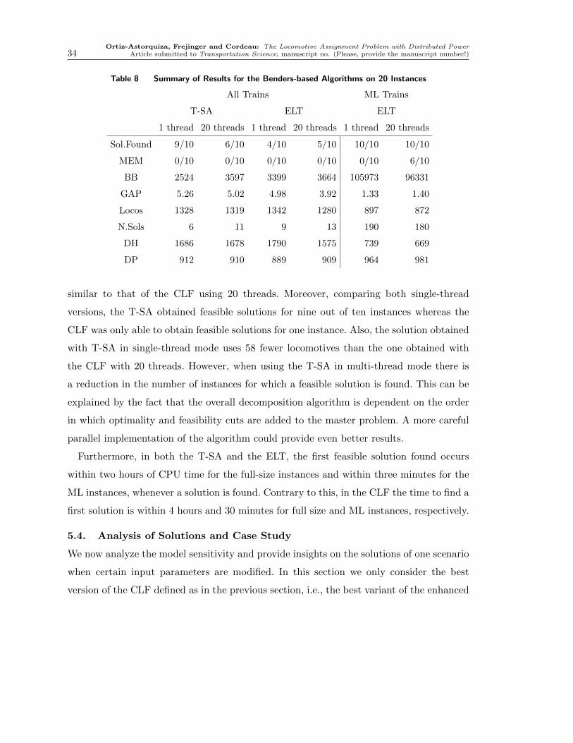
Ortiz-Astorquiza, Frejinger and Cordeau: The Locomotive Assignment Problem with Distributed Power34 Article submitted to Transportation Science; manuscript no. (Please, provide the manuscript number!)
Table 8 Summary of Results for the Benders-based Algorithms on 20 Instances
All Trains ML Trains
T-SA ELT ELT
1 thread 20 threads 1 thread 20 threads 1 thread 20 threads
Sol.Found 9/10 6/10 4/10 5/10 10/10 10/10
MEM 0/10 0/10 0/10 0/10 0/10 6/10
BB 2524 3597 3399 3664 105973 96331
GAP 5.26 5.02 4.98 3.92 1.33 1.40
Locos 1328 1319 1342 1280 897 872
N.Sols 6 11 9 13 190 180
DH 1686 1678 1790 1575 739 669
DP 912 910 889 909 964 981
similar to that of the CLF using 20 threads. Moreover, comparing both single-thread
versions, the T-SA obtained feasible solutions for nine out of ten instances whereas the
CLF was only able to obtain feasible solutions for one instance. Also, the solution obtained
with T-SA in single-thread mode uses 58 fewer locomotives than the one obtained with
the CLF with 20 threads. However, when using the T-SA in multi-thread mode there is
a reduction in the number of instances for which a feasible solution is found. This can be
explained by the fact that the overall decomposition algorithm is dependent on the order
in which optimality and feasibility cuts are added to the master problem. A more careful
parallel implementation of the algorithm could provide even better results.
Furthermore, in both the T-SA and the ELT, the first feasible solution found occurs
within two hours of CPU time for the full-size instances and within three minutes for the
ML instances, whenever a solution is found. Contrary to this, in the CLF the time to find a
first solution is within 4 hours and 30 minutes for full size and ML instances, respectively.
5.4. Analysis of Solutions and Case Study
We now analyze the model sensitivity and provide insights on the solutions of one scenario
when certain input parameters are modified. In this section we only consider the best
version of the CLF defined as in the previous section, i.e., the best variant of the enhanced

Ortiz-Astorquiza, Frejinger and Cordeau: The Locomotive Assignment Problem with Distributed PowerArticle submitted to Transportation Science; manuscript no. (Please, provide the manuscript number!) 35
CLF. In some cases, we also compare the solutions obtained with those of the railway
company. However, we must be careful when comparing these solutions because the LAP-
DP solution is at the tactical level while the historical data used for comparison corresponds
to actual operations. A more fair comparison would be done between a combined solution
of the LAP-DP with the corresponding LRP-DP and the actual operations. But even then,
some characteristics such as repetitiveness of the LAP-DP solution or the implicit handling
of preferences are difficult to compare with the historical data. Nevertheless, for assessing
the quality of solutions obtained in terms of main costs and given the scope of this paper
we use certain statistics from actual operations as benchmark.
In particular, we consider the following values from actual operations. For the all-trains
scenario in discussion, the total number of locomotives used was 1,850 including 200 foreign
power locomotives. The numbers of DH locomotives and light travel trains as well as the
percentages of trains operated on DP, AC-DC and AC-only consists were roughly 950, 25,
7%, 10% and 9%, respectively. It is important to highlight that the solutions obtained
with the model are expected to have more repositioning of locomotives in comparison
with actual operations for two main reasons. First, in the actual operations there is no
enforcement of the cyclic behavior of the solution which means that the assignment cannot
be repeated every week during a season. Second, since we handle foreign power at the
operational level depending on the information available at the beginning of the week,
it is likely that the LRP-DP yields a solution with fewer locomotives being repositioned.
In other words, some light travel trains or DH locomotives would be replaced by foreign
power at the operational solution if the trade-off is cost-beneficial.
We first show the impact on the solutions when considering DP in the modeling process.
As explained before, in certain cases DP is mandatory because the train is too long or too
heavy to be operated on conventional mode but we will assume for this comparison that we
can omit this requirement. Table 9 summarizes the results obtained for one scenario under
four different configurations: not considering any benefit for using DP or AC-only consists
in the HPT, considering AC-only consist benefits, both benefits with the default set-up
time for DP, and both benefits with a large time for setting up a DP consist. Observe that
solving the model with DP appears to be more difficult but it can provide a significant

Ortiz-Astorquiza, Frejinger and Cordeau: The Locomotive Assignment Problem with Distributed Power36 Article submitted to Transportation Science; manuscript no. (Please, provide the manuscript number!)
reduction in the number of locomotives used and deadheaded. In particular, even when we
consider a large time to set up DP, there is a potential reduction of 6% on the number of
used locomotives when including DP and AC-only benefits versus a conventional approach.
Moreover, note that the increase in the percentages of DP trains and AC-only consists in
comparison with the actual operations is more than 15% in both cases.
Table 9 Comparison of Solutions for one Scenario Under DP Configurations
DP βAl DP tm BB UB Locos DH Gap(%) N.Sols Used AL TrtoTr(%) AC-only (%) DP(%)
All
no no default 4880 16134418 1450 2034 3.81 10 258 29.5 23.9 0.0
no yes default 4811 15492700 1399 1946 4.17 10 273 29.4 22.3 0.0
yes yes double 4923 14901091 1364 1719 4.73 13 272 21.6 24.8 22.3
yes yes default 4871 14684483 1329 1769 4.59 6 295 22.4 24.6 23.2
ML
no no default 88938 12750905 1013 876 1.76 208 220 25.6 36.5 0.0
no yes default 92469 11987380 948 840 1.68 197 220 25.2 37.6 0.0
yes yes double 88176 11342541 901 730 2.03 187 228 8.9 39.6 58.0
yes yes default 121150 11126320 881 706 1.52 116 201 10.0 40.8 59.6
Depending on the willingness of the decision maker to emphasize on certain features of
the locomotive plan, the cost composition of the objective function value may be modified.
In this study, we have assumed a cost configuration in which most of the weight is given to
the total number of used locomotives. All the previous solutions described above considered
such configuration. Figure 2 shows two different configurations. The right hand side graphic
depicts this default version (V0). Observe that 66% of the solution value corresponds to
ownership costs and 23% is associated with the operations of active locomotives. The left
hand side graphic of Figure 2 depicts the cost composition of the solution value obtained
when the ownership cost is modified to be 1/10 of its original value. Then, the highest
weight lies on the operations of active locomotives with 60% of the total cost while the
ownership cost is reduced to account for 19%. This shows an example of how railroads can
use the model to quantify cost trade-offs.
In Table 10 we further extend the analysis on cost configurations by considering five
different versions denoted V1 to V5 in addition to the default one. Moreover, we compare
these versions with the values of actual operations denoted with AO. Version V1 takes

Ortiz-Astorquiza, Frejinger and Cordeau: The Locomotive Assignment Problem with Distributed PowerArticle submitted to Transportation Science; manuscript no. (Please, provide the manuscript number!) 37
23%
2%
4%
3%66%
2%
Op. Active
Op. Dh
Busting
LiArc
Ownership
Penalties andIdle
60%
4%
10%
1%
19%
6%
1/10 Ownership Cost (V2) Regular Ownership Cost (V0)
Figure 2 Composition of Costs in the Objective Function Value
zero value for ownership cost, i.e., all the weight in the objective function is on the other
costs. Version V2 corresponds to the 1/10 of ownership cost variant described above. In
versions V3, V4 and V5 we take the same ownership cost as in V2 but include different
penalty costs on DH locomotives and in V5 we use fixed costs on light travel arcs.
Note that in version V1 there is an increase in the number of locomotives used compared
to the other versions because there are no ownership costs. However, it provides insights
on what is the minimum number of light traveling trains that satisfy the requirements.
Also, as we increase the penalty costs for DH locomotives in version V2 to V5, the model
chooses to use less DH at the expense of using more locomotives and more light travel
trains. Recall that in the approximation of light travel costs we implicitly include a penalty
value for discouraging the use of light traveling. This is the reason for the increase in light
travel trains in V5 of the ML instance. Also observe that in all version the percentage of
DP trains is maintained consistently. One important observation is that the default version
V0 showed to be the one for which the solver needed the most CPU time to find a feasible
solution as well as to close the optimality gap, this is one reason for selecting it as the
default configuration as it appeared to be the most computationally challenging.

Ortiz-Astorquiza, Frejinger and Cordeau: The Locomotive Assignment Problem with Distributed Power38 Article submitted to Transportation Science; manuscript no. (Please, provide the manuscript number!)
Table 10 Comparison of Solutions with different Cost Configurations
Version BB Gap(%) Locos Used AL TrtoTr(%) AC-only(%) DC-only (%) DP(%) DH
All
V0 4871 4.59 1329 295 22.4 24.1 75.9 22.7 1769
V1 8028 0.56 1751 35 37.9 17.0 83.0 22.5 1834
V2 1649 2.01 1487 53 33.0 19.9 80.1 22.7 1848
V3 2074 1.97 1477 52 31.7 18.6 81.4 22.7 1655
V4 1529 2.72 1529 60 30.2 19.2 80.8 23.7 1563
V5 1950 - - - - - - - -
AO - - 1850 25 - 9.0 81.0 7.0 950
ML
V0 121150 1.52 881 201 10.0 40.8 59.2 59.6 706
V1 83378 0.05 1279 38 12.2 33.2 66.8 56.4 1137
V2 40177 0.54 998 49 10.8 37.4 62.6 58.6 987
V3 49298 0.37 1009 44 11.4 36.2 63.8 58.8 925
V4 44885 0.73 1026 52 12.2 35.8 64.2 60.6 899
V5 30908 0.68 906 367 11.4 40.5 59.5 59.6 486
Observe from Table 10 that for all six versions, the solutions consistently require fewer
locomotives than the ones used in AO, even if the ownership costs (V1) are set to zero.
Moreover, in all versions we have defined the set of feasible consists in such a way that there
are no AC-DC consists. That is, we have completely removed the 10% of mixed consists
from the solution of actual operations. This in practice is a soft constraint and can be easily
relaxed by including AC-DC consists in the set Cl with penalty values in the objective
function. Also, the solutions obtained with the model show that the percentages of AC-
only and DP consists increase significantly in comparison with those of AO. As mentioned
before, the trade-off occurs with the expected increase in repositioning of locomotives
between the solutions of the CLF and the actual operations. This can be explained with
the cyclic behavior requirements of the model and the foreign power modeling part that
will be treated at the LRP-DP level.
Another parameter that we evaluate is the number of extra DH arcs. Recall that we
control how extra DH arcs are created depending on a threshold value on the number of
inbound or outbound trains at each intermediate station of a train route. This value is
denoted as Thr in Table 11. Thus, given the cost configuration of the model as we increase
the possibility of DH, the solution tends to have more DH locomotives in order to reduce
the number of locomotives used. However, this can be modified according to the planning
preferences and requirements.

Ortiz-Astorquiza, Frejinger and Cordeau: The Locomotive Assignment Problem with Distributed PowerArticle submitted to Transportation Science; manuscript no. (Please, provide the manuscript number!) 39
Table 11 Comparison of Solutions with different Configurations for Extra DH
Extra DH Thr BB Gap(%) Locos Used AL Used AQ(%) AC-only (%) DC-only (%) DP(%) DH
All
no NA 23993 - - - - - - - -
yes 10 4871 4.59 1329 295 22.4 24.1 75.9 22.7 1769
yes 30 4025 4.70 1296 228 21.3 24.1 75.9 22.7 1995
yes 200 4806 4.25 1272 212 20.0 25.2 74.8 23.2 2231
ML
no NA 175704 6.22 973 328 8.7 36.5 63.5 54.6 453
yes 10 121150 1.52 881 201 10.0 40.8 59.2 59.6 706
yes 30 111197 1.09 859 190 8.7 42.3 57.7 59.9 796
yes 200 104781 0.95 856 179 8.3 41.2 58.8 60.3 797
Finally, the model can also be used to identify trade-offs when modifying the size of the
locomotive fleet. For example, managers can receive insights on which types of locomotives
should be bought. In Table 12 we show two examples when +/- 20% of locomotives are
available. On the one hand, as the locomotive fleet becomes larger the enhanced model is
easier to solve which can be exploited in a solution method based on Lagrangean Relax-
ation. On the other hand, when the locomotive fleet is tight to satisfy train requirements
the proposed Benders approach can be used to obtain feasible solutions faster.
Table 12 Comparison of Solutions Considering Different Fleet Size
Fleet Size BB UB Locos DH Gap(%) N.Sols Used AL DP(%)
All
default 4871 14684483 1329 1769 4.59 6 295 23.23
-20% 7950 NA NA NA NA 0 NA NA
+20% 5129 14439899 1308 1735 3.52 18 250 24.98
ML
default 121150 11126320 881 706 1.52 116 201 59.58
-20% 96300 11333270 898 718 2.10 135 214 53.07
+20% 115418 11028619 872 697 1.15 144 202 60.07
6. Conclusions
The purpose of this study was to introduce, model and solve a general tactical-level version
of the LAP in which the operation mode of the trains is part of the decision process. In the
problem definition we also incorporated several real-life aspects based on the requirements
and discussions with the Canadian National Railway Company, one of the largest railway
companies in North America. To model the problem we presented two ILP formulations

Ortiz-Astorquiza, Frejinger and Cordeau: The Locomotive Assignment Problem with Distributed Power40 Article submitted to Transportation Science; manuscript no. (Please, provide the manuscript number!)
that were computationally tested on realistic instances. The results of extensive computa-
tional experiments confirm the efficiency of various enhancements on the CLF model when
solved with a general-purpose solver yielding good solutions in reasonable time. Moreover
the two versions of the Benders-based algorithm showed to significantly reduce the CPU
time to obtain a first solution. Also, the decomposition structure seems well-suited for
problem extensions, in particular those including uncertainty in the parameters.
We also discussed the results obtained with the model and solution approach using dif-
ferent input parameters. Notoriously, even with an optimality gap of over 4%, the enhanced
model provided solutions, under certain costs configurations, where approximately 25%
fewer locomotives are required than those used in actual operations. This major reduction
is a trade-off with the increase in repositioning locomotives in the network but also is
partly explained by the fact that we are comparing at different levels of decision. Thus, care
should be taken to avoid misleading conclusions on solutions that could be more difficult
to comply with at the operational level, especially after when studying other extensions
of the problem that will be the object of subsequent research, for example, concerning
uncertainty. Nevertheless, given the results presented in this article, we believe that the
proposed model is well-suited to provide insights on locomotive planning and that the
potential for cost reduction is very significant.
Acknowledgments
The authors gratefully acknowledge the close collaboration with personnel from the Cana-
dian National Railway Company (CN) and the funding received through the CN Chair in
Optimization of Railway Operations. This research is also funded by the NSERC Collab-
orative Research Grant. Computations were made on the supercomputer beluga, managed
by Calcul Quebec and Compute Canada. The operation of this supercomputer is funded
by the Canada Foundation for Innovation (CFI), the Ministere de l’economie, de la science
et de l’innovation du Quebec (MESI) and the Fonds de recherche du Quebec - Nature et
technologies (FRQ-NT).

Ortiz-Astorquiza, Frejinger and Cordeau: The Locomotive Assignment Problem with Distributed PowerArticle submitted to Transportation Science; manuscript no. (Please, provide the manuscript number!) 41
References
Adulyasak Y, Cordeau JF, Jans R, 2015 Benders decomposition for production routing under
demand uncertainty. Operations Research 63(4):851–867.
Ahuja RK, Liu J, Orlin JB, Sharma D, Shughart LA, 2005 Solving real-life locomotive-scheduling
problems. Transportation Science 39(4):503–517.
Ahuja RK, Magnanti TL, Orlin JB, 1993 Network Flows: Theory, Algorithms, and Applications
(Englewood Cliffs, New Jersey: Prentice Hall).
Benders JF, 1962 Partitioning procedures for solving mixed-variables programming problems.
Numerische Mathematik 4(1):238–252.
Bodur M, Luedtke JR, 2016 Mixed-integer rounding enhanced Benders decomposition for multi-
class service-system staffing and scheduling with arrival rate uncertainty. Management Science
63(7):2073–2091.
Bouzaiene-Ayari B, Cheng C, Das S, Fiorillo R, Powell WB, 2016 From single commodity to mul-
tiattribute models for locomotive optimization: A comparison of optimal integer programming
and approximate dynamic programming. Transportation Science 50(2):366–389.
Cordeau JF, Soumis F, Desrosiers J, 2000 A Benders decomposition approach for the locomotive
and car assignment problem. Transportation Science 34(2):133–149.
Cordeau JF, Soumis F, Desrosiers J, 2001 Simultaneous assignment of locomotives and cars to
passenger trains. Operations Research 49(4):531–548.
Cordeau JF, Toth P, Vigo D, 1998 A survey of optimization models for train routing and scheduling.
Transportation Science 32(4):380–404.
Deveau S, 2011 How long can trains go? National Post URL http://www.nationalpost.com/
long+trains/4348592/story.html.
Fischetti M, Ljubic I, Sinnl M, 2017 Redesigning Benders decomposition for large-scale facility
location. Management Science 63(7):2146–2162.
Florian M, Bushell G, Ferland J, Guerin G, Nastansky L, 1976 The engine scheduling problem in a
railway network. INFOR 14:121–138.
Jaumard B, Tian H, 2016 Multi-column generation model for the locomotive assignment problem.
Goerigk M, Werneck R, eds., OpenAccess Series in Informatics (OASIcs). 16th Workshop on

Ortiz-Astorquiza, Frejinger and Cordeau: The Locomotive Assignment Problem with Distributed Power42 Article submitted to Transportation Science; manuscript no. (Please, provide the manuscript number!)
Algorithmic Approaches for Transportation Modelling, Optimization, and Systems (ATMOS
2016) (Schloss Dagstuhl–Leibniz-Zentrum fuer Informatik. Dagstuhl, Germany).
Magnanti TL, Wong RT, 1981 Accelerating Benders decomposition: Algorithmic enhancement and
model selection criteria. Operations Research 29(3):464–484.
Ortiz-Astorquiza C, Contreras I, Laporte G, 2019 An exact algorithm for multi-level uncapacitated
facility location. Transportation Science 53:1085–1106.
Piu F, Kumar V, Speranza MG, 2015 Introducing a preliminary consists selection in the locomotive
assignment problem. Transportation Research Part E: Logistics and Transportation Review
82:217–237.
Piu F, Speranza MG, 2014 The locomotive assignment problem: A survey on optimization models.
International Transactions in Operational Research 21(3):327–352.
Powell WB, Bouzaiene-Ayari B, Lawrence C, Cheng C, Das S, Fiorillo R, 2014 Locomotive plan-
ning at norfolk southern: An optimizing simulator using approximate dynamic programming.
Interfaces 44(6):567–578.
RAC, 2018 Railway association of Canada. https://www.railcan.ca/101/
delivering-canadas-amazing-products-to-the-world/, [Online; accessed 17-October-
2018].
Rahmaniani R, Crainic TG, Gendreau M, Rei W, 2017 The Benders decomposition algorithm: A
literature review. European Journal of Operational Research 259(3):801–817.
Vaidyanathan B, Ahuja RK, Liu J, Shughart LA, 2008 Real-life locomotive planning: New formula-
tions and computational results. Transportation Research Part B: Methodological 42(2):147–
168.
Vaidyanathan B, Ahuja RK, Orlin JB, 2008 The locomotive routing problem. Transportation Science
42(4):492–507.
Ziarati K, Soumis FF, Desrosiers J, Gelinas S, Saintonge A, 1997 Locomotive assignment with hetero-
geneous consists at CN north america. European Journal of Operational Research 97(2):281–
292.
Ziarati K, Soumis FF, Desrosiers J, Solomon MM, 1999 A branch-first, cut-second approach for
locomotive assignment. Management Science 8(45):1156–1168.