The Local Economic Effectsof Brexit

#CE

PB

RE

XIT

PA

PE

RBR

EXIT10

Swati Dhingra, Stephen Machin and Henry G. Overman

CEP BREXIT ANALYSIS No.10

The Local Economic Effects of Brexit

This paper studies the local impacts of the increases in trade barriers associated with

Brexit. Predictions of the local impact of Brexit are presented under two different

scenarios, soft and hard Brexit.

Average effects are predicted to be negative under both scenarios, and more negative

under hard Brexit. The spatial variation in shocks across areas is somewhat higher under

hard Brexit because some local areas are particularly specialised in sectors that are

predicted to be badly hit by hard Brexit.

Areas in the South of England, and urban areas, are predicted to be harder hit by Brexit

under both scenarios. Again, this pattern is explained by the fact that those areas are

specialised in sectors that are predicted to be badly hit by Brexit.

Finally, the areas that were most likely to vote remain are those that are predicted to be

most negatively impacted by Brexit.

Centre for Economic Performance

London School of Economics and Political Science

Houghton Street, London WC2A 2AE, UK

Tel: +44 (0)20 7955 7673

Email: cep.info@lse.ac.uk Web: http://cep.lse.ac.uk

Acknowledgements and disclaimer:

Thanks to Rui Costa, Nikhil Datta, Hanwei Huang for excellent research assistance. Thanks to

the Centre for Cities for help with the employment data and for providing the Local Authority

and Primary Urban Area maps. The Centre for Economic Performance (CEP) is a politically

independent Research Centre at the London School of Economics. The CEP has no institutional

views, only those of its individual researchers. CEP’s Brexit work is funded by the UK

Economic and Social Research Council. As a whole the CEP, receives less than 5% of its

funding from the European Union. The EU funding is from the European Research Council for

academic projects and not for general funding or consultancy. This work was part funded by

an ESRC Brexit priority grant from UK in a Changing Europe.

1

1. Introduction

In the run up to the UK-EU membership referendum in 2016 a number of studies examined the

potential consequences of Brexit for the UK economy. Most mainstream studies, for example

Dhingra et al. (2016a), HM Treasury (2016) and Kierzenkowski et al., (2016), predicted that

Brexit would have a negative impact on UK GDP. Analysis by the Centre for Economic

Performance, reported in Dhingra et al. (2016a) predicted annual costs of £850 per household

with a ‘soft-Brexit’ and £1,700 per household with a ‘hard Brexit’. Unsurprisingly these

predicted effects are magnified in the long-run (to £4,200 and £6,400 respectively). In the soft

Brexit scenario these results are driven by increases in non-tariff barriers and the exclusion of

the UK from further EU market integration, while allowing for savings in the UK fiscal

contribution to the EU. In the hard Brexit scenario, greater losses occur because of additional

increases in non-tariff barriers, as well as the introduction of bilateral trade tariffs.1

The existing studies examine a number of additional impacts, including foreign investment

(Dhingra et al., 2016b; HM Treasury, 2016; Kierzenkowski et al., 2016), immigration (Dhingra

et al., 2016c; Ebell et al., 2016) and the distributional impacts across income groups (Breinlich

et al. 2016). However, to the best of our knowledge, there exists no regional analysis of the

welfare impacts of Brexit. This short paper provides such an analysis looking at the difference

in predicted effects across all Local Authority Areas and, in an appendix, across Primary Urban

Areas. It also provides some initial analysis on whether these predicted impacts are likely to

exacerbate or alleviate existing disparities.

Predictions on the economic consequences of Brexit are of substantive interest for both central

and local government in understanding how different areas might be affected by Brexit and in

designing the appropriate policy response. There has also been considerable interest in how the

predicted economic impacts of Brexit correlate with voting patterns from the referendum.2 We

provide some analysis that considers this correlation at the area level.

The analysis is based on predictions coming from the methodology applied in Dhingra et al.

(2016a). Their multi sector computable general equilibrium trade model generates sectoral

impacts under different scenarios (i.e. hard and soft Brexit). This state-of-the-art model of the

world economy explains trade patterns well and accounts for the interdependence across

sectors through complex supply chains. Using the most comprehensive data on trade flows and

trade barriers available, their model provides estimates for the impact of different Brexit

scenarios on trade volumes, sectoral production and real economic activity.3 Sectoral impacts

can be weighted using area employment shares to estimate the overall area effect.

These comments notwithstanding, a number of important caveats apply to these results. It is

important to note that the predicted sectoral impacts are model dependent and so we would

urge considerable caution in placing strong weight on the estimated impact for any particular

sector. To give just one example, the model focuses on international trade and will therefore

underestimate losses in sectors, such as air transport, where foreign investment requirements

are more important than trade barriers in determining market access.

1 Precise definitions of these two scenarios are given in Appendix A1. 2 See, for example, some of the contributions in Baldwin (2016) and Becker, Fetzer and Novy (2017). 3 Dhingra et al. allow for multiple sectors and tradeable intermediate inputs and focus on the case of perfect

competition which has been shown to provide a lower bound to the effects of changes in trade costs.

2

It is possible to have more confidence in the area level results, where the employment share

weighting will help ‘wash-out’ some of the sector-specific errors and hopefully give a more

accurate prediction of the area level impacts of increased trade barriers. Even so, it must be

emphasised that these area level results only predict the ‘immediate impact’ based on current

employment shares. Just as with the financial crisis, there are good reasons to think that

adjustment of the spatial economy, will have significant implications for understanding long

run differences in the impact across areas. Future work will need to tackle these issues, but we

believe that there is sufficient interest in understanding the immediate impact to warrant

publication of these predictions.

The results show, as with the previous research, that the average area level effect is negative

under both scenarios and more negative under hard Brexit. This is not surprising given that the

same sectoral effects that underpinned predictions of the national impact are also used to

predict the area level results. Of more interest is the fact that the variability of shocks at the

Local Authority level is considerably higher under hard Brexit (the estimated standard

deviation of spatial shocks being 0.19% for soft Brexit, 0.40% for hard Brexit). This suggests

that some Local Authorities are particularly specialised in sectors that are predicted to be badly

hit by hard Brexit. When looking at Primary Urban Areas average effects are more negative,

consistent with the fact that urban areas have their employment concentrated in the sectors that

are predicted to be most negatively affected. However, the variation under the two different

scenarios is lower (with standard deviations of 0.17% for soft Brexit and 0.35% for hard Brexit)

showing that sectoral diversification can help reduce negative impacts.

The interaction of area level sectoral employment shares with exposure of the relevant sectors

determines the predicted losses for a particular area. Contrary to a small number of existing

studies (see, e.g., Los et al. 2017), areas in London and the South East tend to see bigger

negative impacts. We argue that this difference arises for two reasons. First, because studies

based on measures of current trade exposure to the EU underestimate the importance of

increases in non-tariff barriers (particularly in the hard Brexit scenario). Second, because

simply looking at trade exposure ignores the willingness of individuals and firms to substitute

away from foreign to domestic supply as trade-costs rise. The model in Dhingra et al. (2016a)

accounts for both these factors.

Given these broad geographical patterns, we find that areas that were more likely to vote remain

are those that are predicted to be most negatively impacted by Brexit. Finally, we also find that

the negative impacts of Brexit tend to be bigger for areas with higher average wages. In our

discussion, we highlight the parallel with the financial crisis, and specifically the contrast

between the immediate and long run impacts (which saw London and the South East hit hardest

before recovering much more strongly than other areas of the UK). This suggests that even

though the immediate negative impacts are smaller in poorer regions, households in those areas

start off poorer and may experience considerably more difficulty in adjusting to those negative

shocks.

2. Methodology and Data

Methodology

The underlying methodology for predicting the sectoral impact of Brexit is described in

Dhingra et al. (2016a). They estimate the effect of Brexit on the UK's trade and living standards

3

using a modern quantitative trade model of the global economy. Quantitative trade models

incorporate the channels through which trade affects consumers, firms and workers, and

provide a mapping from trade data to welfare. The model provides predictions for how much

real incomes change under different trade policies, using readily available data on trade

volumes and potential trade barriers. Readers are referred to Dhingra et al. (2016a) for details.

The approach incorporates a broad class of models which make different assumptions about

how goods are produced and how firms compete. It builds on Costinot and Rodríguez-Clare

(2013) who show that some of the most popular trade models predict the same welfare changes

in response to changing trade barriers and that these welfare changes can be computed using

data on trade volumes and trade elasticities.4 Specifically, three pieces of information are used

to predict the impact of the change in trade-costs associated with Brexit: the initial expenditure

shares in each country on each sector, the income levels of different countries and the trade

elasticity (which measures the percentage change in imports relative to domestic demand

resulting from a one percent change in bilateral trade costs, holding incomes constant).5 The

first two of these can be taken from existing data sets, while estimates of the trade elasticity are

available from existing research.

Under the soft Brexit scenario Dhingra et al. (2016a) assume tariffs remain at zero and non-

tariff barriers increase. Tariffs remaining at zero would happen if the UK joins a free trade area,

such as EFTA, with the EU. Non-tariff barriers are the costs arising from customs checks,

border controls, differences in product market regulations, legal barriers and other transactions

costs that make cross-border business more difficult. Even free trade areas cannot eliminate all

the non-tariff barriers that businesses face when transacting across borders. Many non-tariff

barriers arise because countries have different preferences over the regulations that they want

to impose. As a result, trade deals can only reduce that fraction of the non-tariff barriers which

can in principle be eliminated by policy action (so called ‘reducible’ non-tariff barriers).

Berden et al. (2009, 2013) provide detailed calculations of the tariff equivalents of non-tariff

barriers. Under the soft Brexit scenario, Dhingra et al. (2016a) assume that non-tariff barriers

increase: they go up to one quarter of the reducible barriers faced by US exporters to the EU (a

2.77% increase). Given the way in which bilateral trade costs are modelled this increase in non-

tariff barriers (combined with the assumption of no changes in tariff barriers) translates in to a

2.77% increase in bilateral trade costs between the UK and the EU.6

Under the hard Brexit scenario, the UK and the EU are not part of a free trade agreement (at

least immediately) and so they must charge each other the tariffs that they charge to other

members of the World Trade Organization. This means that goods crossing the UK-EU border

are faced with WTO Most-Favoured-Nation tariffs. Dhingra et al. (2016a) also assume that

non-tariff barriers will be larger in the absence of a free trade agreement. Specifically, they are

assumed to increase to three quarters of the reducible barriers faced by US exporters to the EU

(an 8.31% increase).7

4 The paper is available at https://economics.mit.edu/files/9960. 5 For example, the Chemicals and Chemical Products sector has a trade elasticity of 4.75. This means a 10%

increase in tariff in this sector between two countries would translate into a 0.475% reduction in the value of

bilateral trade, holding fixed all economy-wide outcomes across countries. 6 The model assumes frictional barriers of the iceberg type – i.e. Country i has to ship 𝜏ij ≥1 units of its good for

one unit to reach country j. Denoting (MFN) tariffs by tij the effect of increasing tariffs and frictional barriers is

to increase import prices at destination, which are given by Pij=(1+ tij) 𝜏ijPii. 7 See footnote 6 for an explanation of how trade costs are modelled.

4

With the change in bilateral trade costs specified, the model provides a way of simultaneously

estimating the impact on bilateral trade volumes for each sector, taking into account all inter-

sectoral linkages through supply chains and all inter-country linkages through diversion of

trade to other countries. As there are multiple sectors, the model accounts for how changes in

trade costs in intermediate input sectors affect the bilateral trade volumes of the final goods

sector. As there are more than two countries, the model also accounts for how a rise in bilateral

trade costs with one trade partner (in this case the EU) could also lead to a rise in bilateral trade

for countries for whom the trade costs have not changed (i.e. among countries outside the EU).

The trade model provides a logical aggregation of these different interlinkages across sectors

and countries, which gives a set of predictions about what will happen to specific industries in

the two different Brexit scenarios. To get the area level predictions, we simply multiple these

predicted industry specific changes by the employment share of the industry in an area and sum

across industries.8

Data

The national level trade flows and tariff data for each sector-country pair are taken from UN

Comtrade9 and the inter-industry linkages are taken from the World Input-Output Database.10

The latter data set can be used to calculate the initial expenditure shares in each country on

each sector and the income levels of different countries. The trade elasticities that are used to

translate the changes in trade-costs into effects on economic activity are taken from Caliendo

and Parro (2015). As their estimated trade elasticity for the coke, refined petroleum and nuclear

fuel sector is the highest, we re-estimate the sectoral effects in Dhingra et al. (2016a) setting

the changes in this sector to zero. Our results therefore focus on the non-oil sector of the UK

economy.11

The hard Brexit scenario uses Most Favoured Nation (MFN) tariffs at the WIOD sector level

for both UK and EU imports and exports. These are calculated as weighted averages of the

MFN tariffs reported in the World Trade Organisation (WTO) Statistics database,12 with

weights taken from the WIOD and UN Comtrade databases.

Employment shares are calculated based on data from the Business Register and Employment

Survey (BRES) mapped from 2007 SIC 5-digit level to SIC 2003 and then aggregated to the

31 WIOD industries. Employment shares are calculated based on reported data in 2015 so as

to avoid possible employment decisions undertaken by firms as adjustment to the EU

Referendum result of June 2016.

8 Formally, the area level shock is calculated as:

r ir iShock = Employment Share National ShockN

i , where i

stands for industry (i = 1, 2, ……N) and r stands for Local Authority r. 9 See https://comtrade.un.org/. 10 See Timmer et al. (2015) for details. 11 The trade elasticities are sectoral specific for goods sectors, but the same for all service sectors (set equal to 5). 12 http://stat.wto.org/Home/WSDBHome.aspx.

5

3. Results

Sector Predictions

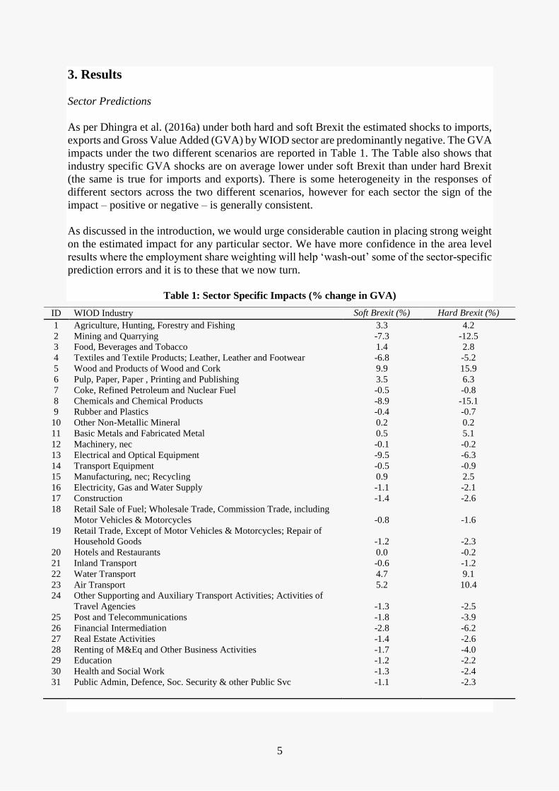
As per Dhingra et al. (2016a) under both hard and soft Brexit the estimated shocks to imports,

exports and Gross Value Added (GVA) by WIOD sector are predominantly negative. The GVA

impacts under the two different scenarios are reported in Table 1. The Table also shows that

industry specific GVA shocks are on average lower under soft Brexit than under hard Brexit

(the same is true for imports and exports). There is some heterogeneity in the responses of

different sectors across the two different scenarios, however for each sector the sign of the

impact – positive or negative – is generally consistent.

As discussed in the introduction, we would urge considerable caution in placing strong weight

on the estimated impact for any particular sector. We have more confidence in the area level

results where the employment share weighting will help ‘wash-out’ some of the sector-specific

prediction errors and it is to these that we now turn.

Table 1: Sector Specific Impacts (% change in GVA)

ID WIOD Industry Soft Brexit (%) Hard Brexit (%)

1 Agriculture, Hunting, Forestry and Fishing 3.3 4.2

2 Mining and Quarrying -7.3 -12.5

3 Food, Beverages and Tobacco 1.4 2.8

4 Textiles and Textile Products; Leather, Leather and Footwear -6.8 -5.2

5 Wood and Products of Wood and Cork 9.9 15.9

6 Pulp, Paper, Paper , Printing and Publishing 3.5 6.3

7 Coke, Refined Petroleum and Nuclear Fuel -0.5 -0.8

8 Chemicals and Chemical Products -8.9 -15.1

9 Rubber and Plastics -0.4 -0.7

10 Other Non-Metallic Mineral 0.2 0.2

11 Basic Metals and Fabricated Metal 0.5 5.1

12 Machinery, nec -0.1 -0.2

13 Electrical and Optical Equipment -9.5 -6.3

14 Transport Equipment -0.5 -0.9

15 Manufacturing, nec; Recycling 0.9 2.5

16 Electricity, Gas and Water Supply -1.1 -2.1

17 Construction -1.4 -2.6

18 Retail Sale of Fuel; Wholesale Trade, Commission Trade, including

Motor Vehicles & Motorcycles -0.8 -1.6

19 Retail Trade, Except of Motor Vehicles & Motorcycles; Repair of

Household Goods -1.2 -2.3

20 Hotels and Restaurants 0.0 -0.2

21 Inland Transport -0.6 -1.2

22 Water Transport 4.7 9.1

23 Air Transport 5.2 10.4

24 Other Supporting and Auxiliary Transport Activities; Activities of

Travel Agencies -1.3 -2.5

25 Post and Telecommunications -1.8 -3.9

26 Financial Intermediation -2.8 -6.2

27 Real Estate Activities -1.4 -2.6

28 Renting of M&Eq and Other Business Activities -1.7 -4.0

29 Education -1.2 -2.2

30 Health and Social Work -1.3 -2.4

31 Public Admin, Defence, Soc. Security & other Public Svc -1.1 -2.3

6

Impact across Local Authority Areas

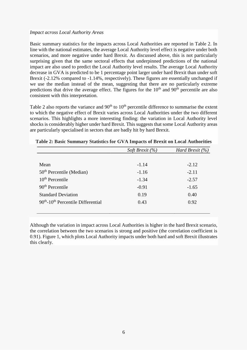
Basic summary statistics for the impacts across Local Authorities are reported in Table 2. In

line with the national estimates, the average Local Authority level effect is negative under both

scenarios, and more negative under hard Brexit. As discussed above, this is not particularly

surprising given that the same sectoral effects that underpinned predictions of the national

impact are also used to predict the Local Authority level results. The average Local Authority

decrease in GVA is predicted to be 1 percentage point larger under hard Brexit than under soft

Brexit (-2.12% compared to -1.14%, respectively). These figures are essentially unchanged if

we use the median instead of the mean, suggesting that there are no particularly extreme

predictions that drive the average effect. The figures for the 10th and 90th percentile are also

consistent with this interpretation.

Table 2 also reports the variance and 90th to 10th percentile difference to summarise the extent

to which the negative effect of Brexit varies across Local Authorities under the two different

scenarios. This highlights a more interesting finding: the variation in Local Authority level

shocks is considerably higher under hard Brexit. This suggests that some Local Authority areas

are particularly specialised in sectors that are badly hit by hard Brexit.

Table 2: Basic Summary Statistics for GVA Impacts of Brexit on Local Authorities

Although the variation in impact across Local Authorities is higher in the hard Brexit scenario,

the correlation between the two scenarios is strong and positive (the correlation coefficient is

0.91). Figure 1, which plots Local Authority impacts under both hard and soft Brexit illustrates

this clearly.

Soft Brexit (%) Hard Brexit (%)

Mean -1.14 -2.12

50th Percentile (Median) -1.16 -2.11

10th Percentile -1.34 -2.57

90th Percentile -0.91 -1.65

Standard Deviation 0.19 0.40

90th-10th Percentile Differential 0.43 0.92

7

Figure 1: Impact of Brexit under Two Different Scenarios

Impact on Specific Local Authorities

We now turn to the impact on specific Local Authorities. Table 3 provides a list of the top ten

most and least affected Local Authorities under the hard Brexit scenario. The results for all

Local Authorities are provided in Table A1 in Appendix A2. Three of the most negatively

affected Local Authorities are within the Greater London area (City of London, Tower Hamlets

and Islington). With the exception of Aberdeen, all the most negatively affected Local

Authorities are in the South of England. Most of these areas have high employment shares in

Business Activities or Financial Intermediation (or both) and so are particularly badly hit by

the large negative effects predicted for those sectors under hard Brexit. For example, the City

of London, which is predicted to see the largest decrease in GVA under a hard Brexit (-4.3%)

had close to 80% of its employed population working in these two sectors as of 2015.

8

Table 3: Most and Least Affected Local Authorities (% Change in Gross Value Added)

Top 10 Soft Brexit

(%)

Hard

Brexit

(%)

Bottom 10 Soft Brexit

(%)

Hard

Brexit

(%)

City of London -1.9 -4.3 Eden -0.7 -1.3

Aberdeen City -2.1 -3.7 Moray -0.7 -1.3

Tower Hamlets -1.7 -3.6 North

Lincolnshire -0.8 -1.3

Watford -1.5 -3.1 Corby -0.8 -1.3

Mole Valley -1.5 -3.0 Anglesey -0.6 -1.2

East Hertfordshire -1.5 -2.8 South Holland -0.6 -1.1

Reading -1.4 -2.8 Crawley -0.7 -1.1

Reigate and

Banstead -1.4 -2.8 Isles of Scilly -0.5 -1.1

Worthing -1.5 -2.8 Melton -0.4 -0.8

Islington -1.3 -2.8 Hounslow -0.2 -0.5

The ten least negatively affected regions show somewhat more geographical variation,

although it is striking that the South of England is now somewhat under-represented.

Hounslow and Crawley do relatively well because their proximity to Heathrow and Gatwick means a high share of employment in the Air Transport Industry, which sees only small loses

even under hard Brexit.13

13 Remember however that the model focuses on international trade and, as noted in the introduction, will therefore

underestimate losses in sectors, such as air transport, where foreign investment requirements are more important

than trade barriers in determining market access.

9

Figure 2: Maps of Percentage Decreases in Local Authority GVA

Figure 2 shows that these findings generalise when we look at the effect across all Local

Authorities. The figure maps the percentage change in GVA by Local Authority under both

soft and hard Brexit. The general geographical patterns are highly similar across both scenarios.

A broad north south pattern is visible, especially in terms of the concentration of areas most

negatively affected. The pattern for those less badly effected is more dispersed. The map also

suggests that urban Local Authorities tend to be more negatively affected (consistent with their

employment concentration in the most negatively affected sectors). Results for Primary Urban

Areas, reported in Appendix A2, confirm that this is the case.

These overall patterns deviate markedly from a small number of existing studies (see, e.g., Los

et al. 2017) which suggest that impacts are likely to be biggest outside of the South of England.

Two factors would appear to explain these differences. First, existing studies are based on

measures of trade exposure to the EU, which is larger for areas outside of the South of England.

However, these measures of current exposure underestimate the importance of increases in

non-tariff barriers (particularly in the hard Brexit scenario). Second, simply looking at trade

exposure ignores the willingness of individuals and firms to substitute away from foreign to

domestic supply as trade-costs rise. These substitution effects are largest in service industries

that are concentrated in the South of England (and Primary Urban Areas). The model accounts

for both these factors and thus predicts a strikingly different pattern in terms of those areas

predicted to be most negatively affected by Brexit.

10

4. Correlations with Brexit Vote and Area Initial Conditions

Brexit Vote Correlations

One obvious question arising from the overall patterns discussed above is how predicted

impacts relate to vote shares in the referendum. Figure 3 provides an answer: areas that are

predicted to be most negatively affected by Brexit were more likely to vote remain. The

correlation is particularly striking for the predicted impacts under hard Brexit (correlation of -

0.39 for hard Brexit as opposed to -0.24 for soft Brexit). Again, this finding differs from some

existing studies because of the different geographical pattern for the places that are predicted

to experience the most negative impacts from hard Brexit.

Figure 3: Brexit GVA Impact and Referendum Vote Share

(a): Soft Brexit (b) Hard Brexit

Area Initial Conditions

While the results so far imply a somewhat different narrative in terms of who is likely to lose

most from Brexit, and how this relates to voting behaviour in the referendum, it is important to

remember that the differences in expected impacts are swamped by existing disparities. Even

though the immediate negative impacts are predicted to be smaller in poorer regions,

households in those areas start off poorer and may experience considerably more difficulty in

adjusting to those negative shocks. This is shown for the example of one initial condition,

median wage levels, in Figure 4 (the correlation is -0.23 for soft Brexit, -0.37 for hard Brexit).

11

Figure 4: Correlation of Brexit GVA Impact with Pre-Referendum Median Wage

(a): Soft Brexit (b) Hard Brexit

Finally, it is also important to note that the places experiencing the biggest initial shock are not

necessarily those that will experience the most negative effects once the economy has adjusted.

As discussed in the introduction, we would highlight the parallel with the financial crisis and

specifically the contrast between the immediate and long run impacts (which saw London and

the South East hit hardest before recovering much more strongly than other areas of the UK).

5. Conclusions

This paper has provided predictions of the impact of Brexit across Local Authorities under two

different scenarios. Average effects are predicted to be negative under both scenarios and more

negative under hard Brexit. The variation in shocks across Local Authorities is somewhat

higher under hard Brexit because some Local Authorities are particularly specialised in sectors

that are predicted to be badly hit by hard Brexit.

Local Authorities in the South of England, and those in urban areas, are predicted to be harder

hit by Brexit under both scenarios. Again, this pattern is explained by the fact that those areas

are specialised by sectors that are predicted to be badly hit by Brexit. We find that areas that

were most likely to vote remain are those that are predicted to be most negatively impacted by

Brexit. We also find that the negative impacts of Brexit tend to be bigger for areas with higher

average wages.

The figures in this paper represent a first attempt to look at the Local Authority impacts of the

increases in trade barriers associated with Brexit. Further work will be needed to better

understand these impacts, to understand the impacts working through other channels, such as

migration and investment, and to understand the longer run impacts as the economy adjusts. In

short, these figures are far from the last word, but they do provide an initial indication of the

way in which the impact of Brexit may be felt differently across the areas of Great Britain.

July 2017

For further information, contact:

Dr Swati Dhingra, Email: S.Dhingra@lse.ac.uk; Professor Stephen Machin, Email:

s.j.machin@lse.ac.uk’; Professor Henry G. Overman, Email: h.g.overman@lse.ac.uk or

Romesh Vaitilingam, Email: romesh@vaitilingam.com.

12

References

Baldwin, R. (ed.) (2016) Brexit Beckons: Thinking Ahead by Leading Economists, Vox EU

book.

Becker, S., T. Fetzer and D. Novy (2017) ‘Who Voted for Brexit? A Comprehensive District-

Level Analysis’, Centre for Economic Performance Discussion Paper No. 1480, April 2017.

Berden, K., J. Francois, S. Tamminen, M. Thelle and P. Wymenga (2009) ‘Non-Tariff

Measures in EU-US Trade and Investment – An Economic Analysis’, Ecorys report prepared

for the European Commission, Reference OJ 2007/S180219493.

Berden, K., J. Francois, K. Tamminen, M. Thelle and P. Wymenga (2013) ‘Non-tariff Barriers

in EU-US Trade and Investment: An Economic Analysis’, Technical Report, Institute for

International and Development Economics.

Breinlich, H. Dhingra, S., T. Sampson and J. Van Reenen (2016) ‘Who Bears the Pain? How

the Costs of Brexit Would be Distributed Across Income Groups’, CEP BREXIT Paper No.

07.

Caliendo, L and F. Parro (2015) Estimates of the Trade and Welfare Effects of NAFTA. The

Review of Economic Studies, 82 (1): 1-44

Costinot, A and A. Rodríguez-Clare (2013) Trade Theory with Numbers: Quantifying the

Consequences of Globalization in Gopinath, G., E. Helpman and K. Rogoff (eds.) Handbook

of International Economics, Elsevier. ISBN: 978-0-444-54314-1.

Dhingra, S., G. Ottaviano, T. Sampson and J. Van Reenen (2016a) ‘The Consequences of

Brexit for UK Trade and Living Standards’, CEP BREXIT Paper No. 02.

Dhingra, S., G. Ottaviano, T. Sampson and J. Van Reenen (2016b) ‘The Impact of Brexit on

Foreign Investment in the UK’, CEP BREXIT Paper No. 03.

Dhingra, S., G. Ottaviano, J. Van Reenen and J. Wadsworth (2016c) ‘Brexit and the Impact of

Immigration on the UK’, CEP BREXIT Paper No. 05.

Ebell, M. and J. Warren (2016) ‘The Long-Term Economic Impact of Leaving the EU’,

National Institute Economic Review 236, 121-138.

Ebell M, I. Hurst and J. Warren (2016) ‘Modelling the Long-run Economic Impact of Leaving

the European Union’, NIESR Discussion Paper No. 462.

HM Treasury (2016) ‘The Long-Term Economic Impact of EU Membership and the

Alternatives’, ISBN 978-1-4741-3090-5.

Kierzenkowski, R., N. Pain, E. Rusticelli and S. Zwart (2016) ‘The Economic Consequences

of Brexit: A Taxing Decision’, OECD Economic Policy Papers, No. 16, OECD Publishing,

Paris. http://dx.doi.org/10.1787/5jm0lsvdkf6k-en

13

Los, B., P. McCann, J. Springford and M. Thissen (2017) ‘The Mismatch Between Local

Voting and the Local Economic Consequences of Brexit’. Regional Studies 51(5).

Méjean, I. and C. Schwellnus (2009) ‘Price convergence in the European Union: Within firms

or composition of firms?’ Journal of International Economics, 78(1), 1-10.

Timmer, M. P., Dietzenbacher, E., Los, B., Stehrer, R. and de Vries, G. J. (2015) ‘An Illustrated

User Guide to the World Input–Output Database: the Case of Global Automotive Production’,

Review of International Economics, 23: 575–605.

14

Appendices

Appendix A1: Hard and Soft Brexit and Timescales

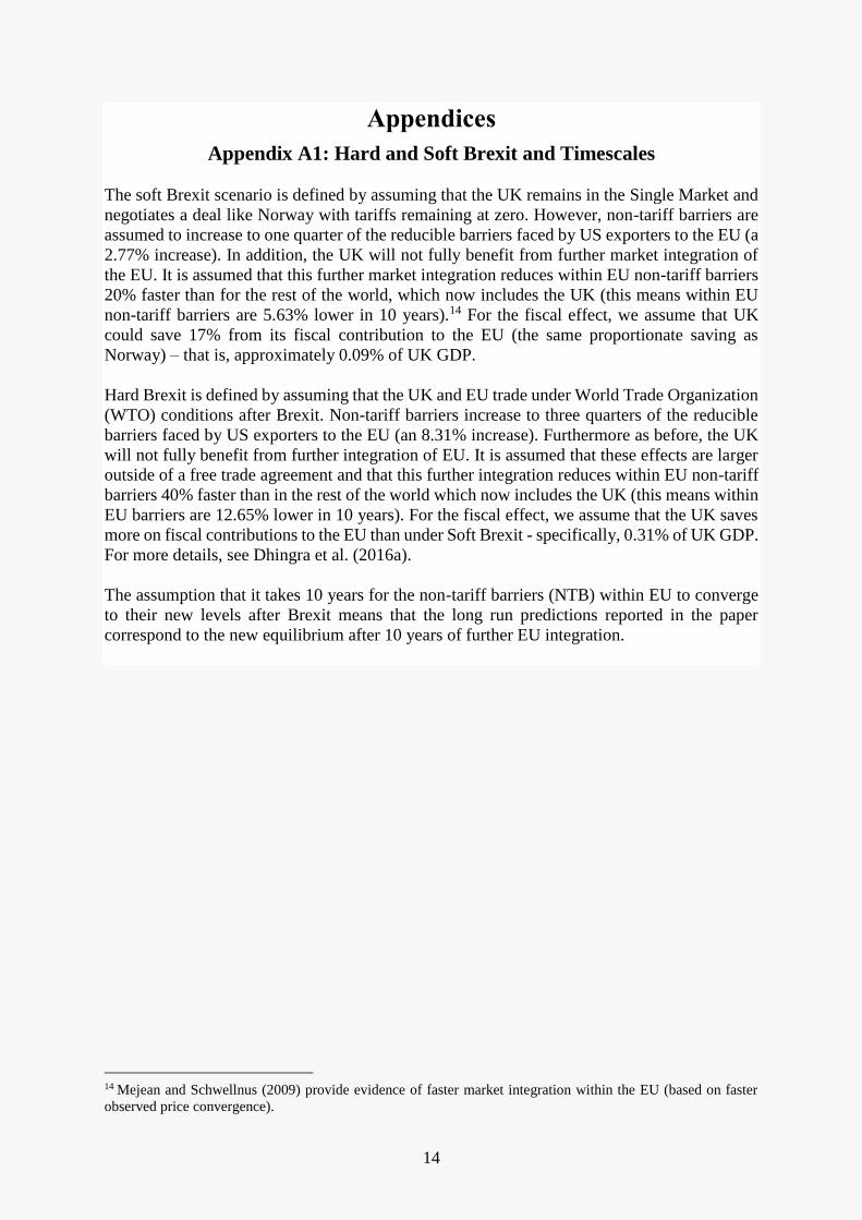
The soft Brexit scenario is defined by assuming that the UK remains in the Single Market and

negotiates a deal like Norway with tariffs remaining at zero. However, non-tariff barriers are

assumed to increase to one quarter of the reducible barriers faced by US exporters to the EU (a

2.77% increase). In addition, the UK will not fully benefit from further market integration of

the EU. It is assumed that this further market integration reduces within EU non-tariff barriers

20% faster than for the rest of the world, which now includes the UK (this means within EU

non-tariff barriers are 5.63% lower in 10 years).14 For the fiscal effect, we assume that UK

could save 17% from its fiscal contribution to the EU (the same proportionate saving as

Norway) – that is, approximately 0.09% of UK GDP.

Hard Brexit is defined by assuming that the UK and EU trade under World Trade Organization

(WTO) conditions after Brexit. Non-tariff barriers increase to three quarters of the reducible

barriers faced by US exporters to the EU (an 8.31% increase). Furthermore as before, the UK

will not fully benefit from further integration of EU. It is assumed that these effects are larger

outside of a free trade agreement and that this further integration reduces within EU non-tariff

barriers 40% faster than in the rest of the world which now includes the UK (this means within

EU barriers are 12.65% lower in 10 years). For the fiscal effect, we assume that the UK saves

more on fiscal contributions to the EU than under Soft Brexit - specifically, 0.31% of UK GDP.

For more details, see Dhingra et al. (2016a).

The assumption that it takes 10 years for the non-tariff barriers (NTB) within EU to converge

to their new levels after Brexit means that the long run predictions reported in the paper

correspond to the new equilibrium after 10 years of further EU integration.

14 Mejean and Schwellnus (2009) provide evidence of faster market integration within the EU (based on faster

observed price convergence).

15

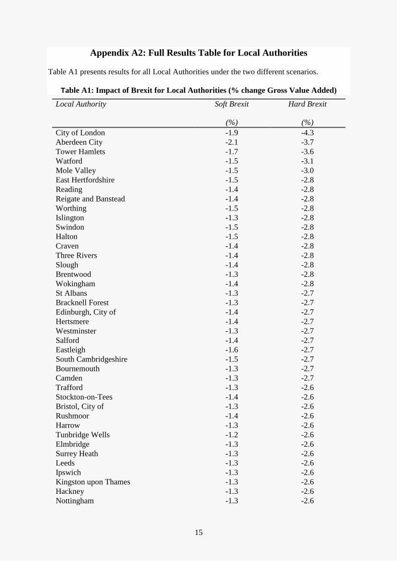
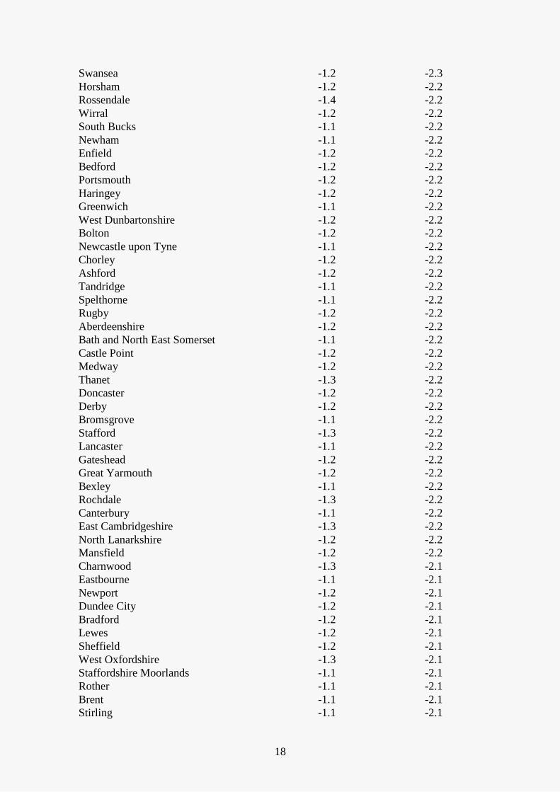
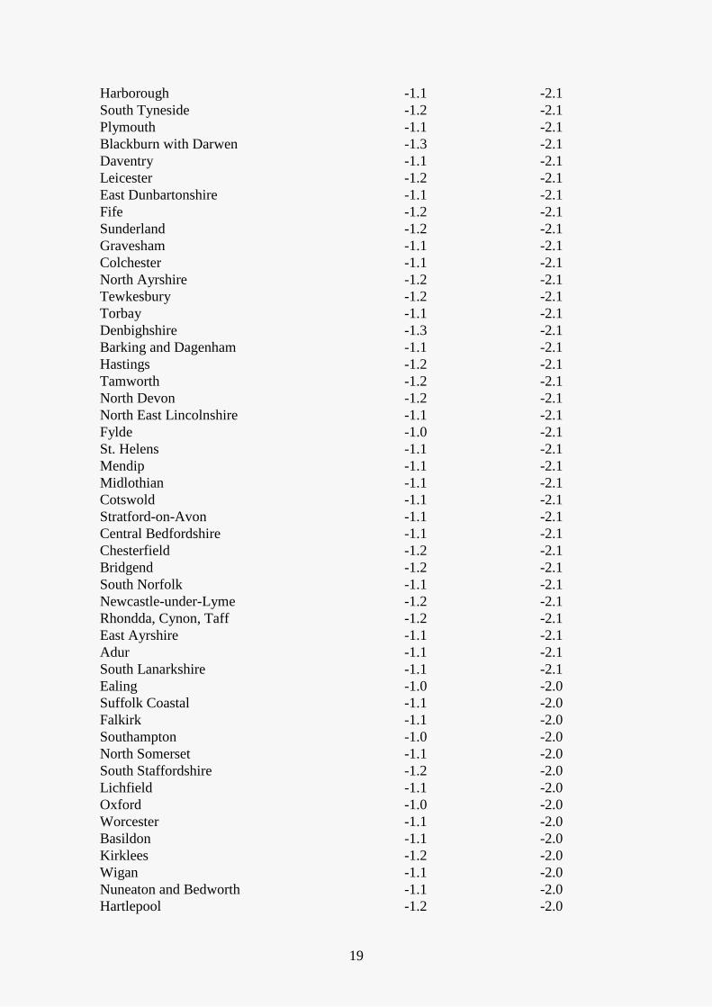
Appendix A2: Full Results Table for Local Authorities

Table A1 presents results for all Local Authorities under the two different scenarios.

Table A1: Impact of Brexit for Local Authorities (% change Gross Value Added)

Local Authority Soft Brexit

(%)

Hard Brexit

(%)

City of London -1.9 -4.3

Aberdeen City -2.1 -3.7

Tower Hamlets -1.7 -3.6

Watford -1.5 -3.1

Mole Valley -1.5 -3.0

East Hertfordshire -1.5 -2.8

Reading -1.4 -2.8

Reigate and Banstead -1.4 -2.8

Worthing -1.5 -2.8

Islington -1.3 -2.8

Swindon -1.5 -2.8

Halton -1.5 -2.8

Craven -1.4 -2.8

Three Rivers -1.4 -2.8

Slough -1.4 -2.8

Brentwood -1.3 -2.8

Wokingham -1.4 -2.8

St Albans -1.3 -2.7

Bracknell Forest -1.3 -2.7

Edinburgh, City of -1.4 -2.7

Hertsmere -1.4 -2.7

Westminster -1.3 -2.7

Salford -1.4 -2.7

Eastleigh -1.6 -2.7

South Cambridgeshire -1.5 -2.7

Bournemouth -1.3 -2.7

Camden -1.3 -2.7

Trafford -1.3 -2.6

Stockton-on-Tees -1.4 -2.6

Bristol, City of -1.3 -2.6

Rushmoor -1.4 -2.6

Harrow -1.3 -2.6

Tunbridge Wells -1.2 -2.6

Elmbridge -1.3 -2.6

Surrey Heath -1.3 -2.6

Leeds -1.3 -2.6

Ipswich -1.3 -2.6

Kingston upon Thames -1.3 -2.6

Hackney -1.3 -2.6

Nottingham -1.3 -2.6

16

Basingstoke and Deane -1.4 -2.6

Northampton -1.3 -2.6

Bromley -1.3 -2.6

Hart -1.4 -2.6

Epsom and Ewell -1.2 -2.6

Chiltern -1.3 -2.5

Vale of White Horse -1.4 -2.5

Milton Keynes -1.3 -2.5

Southwark -1.2 -2.5

Windsor and Maidenhead -1.3 -2.5

Cheshire West and Chester -1.3 -2.5

Lambeth -1.2 -2.5

Runnymede -1.2 -2.5

Brighton and Hove -1.3 -2.5

Glasgow City -1.3 -2.5

South Oxfordshire -1.3 -2.5

Woking -1.3 -2.5

Broxbourne -1.3 -2.5

Cardiff -1.3 -2.5

Welwyn Hatfield -1.3 -2.5

Guildford -1.3 -2.5

Havant -1.5 -2.5

Dacorum -1.3 -2.5

Croydon -1.2 -2.5

Merton -1.2 -2.5

Cheshire East -1.3 -2.5

Warrington -1.3 -2.5

Redbridge -1.2 -2.5

Manchester -1.2 -2.5

Barnet -1.2 -2.5

Peterborough -1.2 -2.5

Cambridge -1.3 -2.5

South Gloucestershire -1.3 -2.5

North Tyneside -1.3 -2.5

Blaby -1.3 -2.5

Dartford -1.3 -2.5

Gloucester -1.4 -2.5

Poole -1.4 -2.4

Chelmsford -1.3 -2.4

Wandsworth -1.2 -2.4

Waverley -1.2 -2.4

Broxtowe -1.3 -2.4

Exeter -1.2 -2.4

Harlow -1.4 -2.4

Winchester -1.3 -2.4

Stockport -1.3 -2.4

Inverclyde -1.3 -2.4

Cheltenham -1.2 -2.4

Southend-on-Sea -1.3 -2.4

17

Darlington -1.2 -2.4

Fareham -1.4 -2.4

Preston -1.2 -2.4

Liverpool -1.2 -2.4

East Hampshire -1.3 -2.4

Richmond upon Thames -1.1 -2.4

Bury -1.3 -2.4

St Edmundsbury -1.3 -2.4

Stevenage -1.3 -2.4

Calderdale -1.3 -2.4

Hammersmith and Fulham -1.1 -2.4

Middlesbrough -1.2 -2.4

West Lothian -1.3 -2.4

Mid Sussex -1.2 -2.3

Lewisham -1.2 -2.3

West Berkshire -1.2 -2.3

Maidstone -1.2 -2.3

Warwick -1.2 -2.3

Bolsover -1.2 -2.3

Sefton -1.2 -2.3

Taunton Deane -1.2 -2.3

Birmingham -1.2 -2.3

Redcar and Cleveland -1.3 -2.3

Coventry -1.2 -2.3

Sevenoaks -1.2 -2.3

Wycombe -1.2 -2.3

Broadland -1.2 -2.3

North West Leicestershire -1.3 -2.3

Test Valley -1.2 -2.3

Sutton -1.1 -2.3

Havering -1.2 -2.3

Waltham Forest -1.2 -2.3

Epping Forest -1.2 -2.3

Norwich -1.2 -2.3

Thurrock -1.2 -2.3

Shepway -1.2 -2.3

Lincoln -1.2 -2.3

Knowsley -1.2 -2.3

Solihull -1.1 -2.3

Tonbridge and Malling -1.1 -2.3

North Hertfordshire -1.3 -2.3

The Vale of Glamorgan -1.3 -2.3

East Renfrewshire -1.2 -2.3

Wiltshire -1.2 -2.3

York -1.1 -2.3

Renfrewshire -1.3 -2.3

Rushcliffe -1.1 -2.3

Harrogate -1.1 -2.3

Aylesbury Vale -1.2 -2.3

18

Swansea -1.2 -2.3

Horsham -1.2 -2.2

Rossendale -1.4 -2.2

Wirral -1.2 -2.2

South Bucks -1.1 -2.2

Newham -1.1 -2.2

Enfield -1.2 -2.2

Bedford -1.2 -2.2

Portsmouth -1.2 -2.2

Haringey -1.2 -2.2

Greenwich -1.1 -2.2

West Dunbartonshire -1.2 -2.2

Bolton -1.2 -2.2

Newcastle upon Tyne -1.1 -2.2

Chorley -1.2 -2.2

Ashford -1.2 -2.2

Tandridge -1.1 -2.2

Spelthorne -1.1 -2.2

Rugby -1.2 -2.2

Aberdeenshire -1.2 -2.2

Bath and North East Somerset -1.1 -2.2

Castle Point -1.2 -2.2

Medway -1.2 -2.2

Thanet -1.3 -2.2

Doncaster -1.2 -2.2

Derby -1.2 -2.2

Bromsgrove -1.1 -2.2

Stafford -1.3 -2.2

Lancaster -1.1 -2.2

Gateshead -1.2 -2.2

Great Yarmouth -1.2 -2.2

Bexley -1.1 -2.2

Rochdale -1.3 -2.2

Canterbury -1.1 -2.2

East Cambridgeshire -1.3 -2.2

North Lanarkshire -1.2 -2.2

Mansfield -1.2 -2.2

Charnwood -1.3 -2.1

Eastbourne -1.1 -2.1

Newport -1.2 -2.1

Dundee City -1.2 -2.1

Bradford -1.2 -2.1

Lewes -1.2 -2.1

Sheffield -1.2 -2.1

West Oxfordshire -1.3 -2.1

Staffordshire Moorlands -1.1 -2.1

Rother -1.1 -2.1

Brent -1.1 -2.1

Stirling -1.1 -2.1

19

Harborough -1.1 -2.1

South Tyneside -1.2 -2.1

Plymouth -1.1 -2.1

Blackburn with Darwen -1.3 -2.1

Daventry -1.1 -2.1

Leicester -1.2 -2.1

East Dunbartonshire -1.1 -2.1

Fife -1.2 -2.1

Sunderland -1.2 -2.1

Gravesham -1.1 -2.1

Colchester -1.1 -2.1

North Ayrshire -1.2 -2.1

Tewkesbury -1.2 -2.1

Torbay -1.1 -2.1

Denbighshire -1.3 -2.1

Barking and Dagenham -1.1 -2.1

Hastings -1.2 -2.1

Tamworth -1.2 -2.1

North Devon -1.2 -2.1

North East Lincolnshire -1.1 -2.1

Fylde -1.0 -2.1

St. Helens -1.1 -2.1

Mendip -1.1 -2.1

Midlothian -1.1 -2.1

Cotswold -1.1 -2.1

Stratford-on-Avon -1.1 -2.1

Central Bedfordshire -1.1 -2.1

Chesterfield -1.2 -2.1

Bridgend -1.2 -2.1

South Norfolk -1.1 -2.1

Newcastle-under-Lyme -1.2 -2.1

Rhondda, Cynon, Taff -1.2 -2.1

East Ayrshire -1.1 -2.1

Adur -1.1 -2.1

South Lanarkshire -1.1 -2.1

Ealing -1.0 -2.0

Suffolk Coastal -1.1 -2.0

Falkirk -1.1 -2.0

Southampton -1.0 -2.0

North Somerset -1.1 -2.0

South Staffordshire -1.2 -2.0

Lichfield -1.1 -2.0

Oxford -1.0 -2.0

Worcester -1.1 -2.0

Basildon -1.1 -2.0

Kirklees -1.2 -2.0

Wigan -1.1 -2.0

Nuneaton and Bedworth -1.1 -2.0

Hartlepool -1.2 -2.0

20

Oldham -1.2 -2.0

Scottish Borders -1.2 -2.0

Arun -1.2 -2.0

North Warwickshire -1.1 -2.0

Wyre -1.1 -2.0

New Forest -1.1 -2.0

Stoke-on-Trent -1.1 -2.0

Cherwell -1.1 -2.0

County Durham -1.2 -2.0

South Ribble -1.1 -2.0

Redditch -1.4 -2.0

Torfaen -1.2 -2.0

Teignbridge -1.1 -2.0

Gwynedd -1.1 -2.0

Weymouth and Portland -1.0 -2.0

Telford and Wrekin -1.1 -2.0

Luton -1.1 -2.0

Babergh -1.2 -2.0

Christchurch -1.2 -2.0

Wyre Forest -1.2 -2.0

East Dorset -1.1 -2.0

Northumberland -1.1 -2.0

Mid Suffolk -1.1 -2.0

South Northamptonshire -1.1 -2.0

Huntingdonshire -1.1 -2.0

Maldon -1.2 -2.0

Malvern Hills -1.1 -1.9

Conwy -1.0 -1.9

Stroud -1.4 -1.9

Wellingborough -1.1 -1.9

Kensington and Chelsea -0.9 -1.9

Blackpool -1.0 -1.9

Burnley -1.1 -1.9

King`s Lynn and West Norfolk -1.0 -1.9

Rochford -1.0 -1.9

Braintree -1.1 -1.9

Walsall -1.2 -1.9

Wakefield -1.1 -1.9

Tendring -1.1 -1.9

Isle of Wight -1.1 -1.9

West Dorset -1.1 -1.9

Highland -1.0 -1.9

East Lothian -1.0 -1.9

Caerphilly -1.2 -1.9

Blaenau Gwent -1.2 -1.9

Purbeck -1.0 -1.9

East Riding of Yorkshire -1.0 -1.9

Chichester -1.0 -1.9

Breckland -1.0 -1.9

21

Perth and Kinross -0.9 -1.9

Swale -1.0 -1.9

Rotherham -1.1 -1.9

Wealden -1.0 -1.9

East Staffordshire -1.0 -1.9

Gedling -1.2 -1.9

Torridge -1.0 -1.9

Clackmannanshire -1.0 -1.9

Wolverhampton -1.1 -1.9

Tameside -1.1 -1.9

Gosport -1.0 -1.9

Rutland -1.1 -1.9

South Hams -1.0 -1.9

South Lakeland -1.1 -1.8

South Ayrshire -1.0 -1.8

Cornwall -0.9 -1.8

Kingston upon Hull, City of -1.0 -1.8

North Dorset -1.2 -1.8

High Peak -1.1 -1.8

Richmondshire -0.9 -1.8

Eilean Siar -0.9 -1.8

Carlisle -1.0 -1.8

Selby -1.1 -1.8

Ceredigion -0.9 -1.8

Ashfield -1.2 -1.8

South Somerset -1.0 -1.8

Kettering -1.0 -1.8

Monmouthshire -1.0 -1.8

Pembrokeshire -1.0 -1.8

Hillingdon -0.9 -1.8

Boston -1.0 -1.8

Angus -1.1 -1.8

East Northamptonshire -1.0 -1.8

Mid Devon -1.1 -1.8

Shropshire -0.9 -1.8

Bassetlaw -1.0 -1.8

West Devon -0.9 -1.8

Hinckley and Bosworth -1.1 -1.7

Derbyshire Dales -1.1 -1.7

East Devon -0.9 -1.7

Dudley -1.0 -1.7

Oadby and Wigston -1.0 -1.7

Cannock Chase -1.0 -1.7

Barrow-in-Furness -1.0 -1.7

South Derbyshire -0.9 -1.7

Barnsley -0.9 -1.7

Wrexham -1.1 -1.7

West Lindsey -0.9 -1.7

Dover -0.9 -1.7

22

Argyll and Bute -0.9 -1.7

Carmarthenshire -1.0 -1.7

Uttlesford -0.9 -1.7

Copeland -0.9 -1.7

South Kesteven -1.0 -1.7

Flintshire -1.0 -1.7

West Lancashire -0.9 -1.7

Scarborough -0.9 -1.7

Ribble Valley -0.9 -1.7

Hyndburn -1.0 -1.6

Sandwell -1.0 -1.6

East Lindsey -0.9 -1.6

Hambleton -0.9 -1.6

Newark and Sherwood -0.9 -1.6

West Somerset -0.8 -1.6

North Kesteven -0.9 -1.6

Powys -1.0 -1.6

North Norfolk -0.8 -1.6

Forest Heath -0.9 -1.6

Orkney Islands -0.8 -1.6

Sedgemoor -0.9 -1.6

Shetland Islands -0.8 -1.6

Wychavon -0.9 -1.6

Erewash -1.0 -1.6

Waveney -0.8 -1.5

Pendle -1.1 -1.5

Merthyr Tydfil -0.8 -1.5

Herefordshire, County of -0.8 -1.5

Dumfries and Galloway -0.7 -1.4

Forest of Dean -0.8 -1.4

Allerdale -0.8 -1.4

Amber Valley -0.9 -1.4

Fenland -0.7 -1.4

Ryedale -0.8 -1.4

Neath Port Talbot -1.0 -1.4

North East Derbyshire -0.9 -1.4

Eden -0.7 -1.3

Moray -0.7 -1.3

North Lincolnshire -0.8 -1.3

Corby -0.8 -1.3

Anglesey -0.6 -1.2

South Holland -0.6 -1.1

Crawley -0.7 -1.1

Isles of Scilly -0.5 -1.1

Melton -0.4 -0.8

Hounslow -0.2 -0.5

23

Appendix A3: Impact of Brexit Across Primary Urban Areas

The results presented in the main body of the text, and in Appendix A2 are for Local

Authorities. These have the advantage that they cover the whole of Great Britain and thus give

an estimate of the impact of Brexit for all areas. However, when large number of households

commute across a Local Authority boundary for work we can get better predictions of the

impact of Brexit on households if we look at the impact on functional economic areas – defined,

somewhat circularly, as the spatial scale at which the relevant economic markets operate. To

take a more concrete example, for a household living in one of our big cities, predictions at the

urban area level are more likely to capture the impact on the income of that household. In this

appendix we present such results for Primary Urban Areas (PUAs), a convenient aggregation

of Local Authorities that better match urban economies than stand-alone Local Authorities.

Basic summary statistics for the impact across PUAs are reported in Table A2. In line with the

national and Local Authority estimates, the average PUA level effect is negative under both

scenarios and more negative under hard Brexit. Comparing to Table 2, we see that the mean

impact for PUAs is somewhat higher than that for Local Authorities, consistent with the

suggestion in the main text that the employment concentration of urban areas mean that they

are predicted to be somewhat harder hit than non-urban areas.

As with Local Authorities, these figures are essentially unchanged if we use the median instead

of the mean, suggesting that there are no particularly extreme predictions that drive the average

effect. The figures for the 10th and 90th percentile are also consistent with this interpretation.

Table A2 also reports the variance and 90th to 10th percentile different to summarise how much

the negative effect of Brexit varies across PUAs under the two different scenarios. As with

Local Authorities, the variation in PUA shocks is considerably higher under hard Brexit. This

suggests that some PUAs are particularly specialised in sectors that are badly hit by hard Brexit.

Having said this, the variation under the two different scenarios is lower for Primary Urban

Areas (0.17% for soft Brexit, 0.35% for hard Brexit) showing the importance of urban

diversification in helping mitigate negative impacts.

24

Table A2: PUA Distribution Statistics of GVA Impacts of Brexit

Table A3 lists the top ten most and least affected PUAs under the hard Brexit scenario. The

results for all PUAs are provided in Table A4. The most affected PUAs show slightly more

geographical diversity in comparison to the most affected Local Authorities (which, with the

exception of Aberdeen were all in the South of England). For the least affected, the under-

representation of the South of England is somewhat more apparent than it was for Local

Authorities. PUAs across Great Britain are hit harder than Local Authorities, but PUAs outside

the South of England tend to be less hard hit than other PUAs. Figure A1 which maps the

percentage change in GVA by PUA under both soft and hard Brexit confirms this broad

geographical pattern.

Table A3: Most and Least Affected Primary Urban Areas

(% Change in Gross Value Added)

Top 10 Soft Brexit

(%)

Hard

Brexit

(%)

Bottom 10 Soft Brexit

(%)

Hard

Brexit

(%)

Aberdeen -2.1 -3.7 Blackpool -1.0 -2.0

Worthing -1.5 -2.8 Swansea -1.1 -2.0

Reading -1.4 -2.8 Telford -1.1 -2.0

Swindon -1.5 -2.8 Luton -1.1 -2.0

Slough -1.4 -2.8 Mansfield -1.2 -2.0

Edinburgh -1.4 -2.7 Wakefield -1.1 -1.9

London -1.3 -2.6 Hull -1.0 -1.8

Aldershot -1.3 -2.6 Burnley -1.1 -1.7

Leeds -1.3 -2.6 Barnsley -0.9 -1.7

Ipswich -1.3 -2.6 Crawley -0.7 -1.1

Soft Brexit

(%)

Hard Brexit

(%)

Mean -1.22 -2.28

50th Percentile (Median) -1.21 -2.26

10th Percentile -1.35 -2.60

90th Percentile -1.07 -1.98

Standard Deviation 0.17 0.35

90th-10th Percentile

Differential 0.28 0.62

25

Table A4: Impact of Brexit for Primary Urban Areas

(% Change in Gross Value Added)

Primary Urban Area Soft Brexit

(%)

Hard Brexit

(%)

Aberdeen -2.1 -3.7

Worthing -1.5 -2.8

Reading -1.4 -2.8

Swindon -1.5 -2.8

Slough -1.4 -2.8

Edinburgh -1.4 -2.7

London -1.3 -2.6

Aldershot -1.3 -2.6

Leeds -1.3 -2.6

Ipswich -1.3 -2.6

Bristol -1.3 -2.6

Northampton -1.3 -2.6

Milton Keynes -1.3 -2.5

Cardiff -1.3 -2.5

Warrington -1.3 -2.5

Middlesbrough -1.3 -2.5

Peterborough -1.2 -2.5

Cambridge -1.3 -2.5

Brighton -1.2 -2.5

Gloucester -1.4 -2.5

Glasgow -1.3 -2.4

Exeter -1.2 -2.4

Bournemouth -1.3 -2.4

Manchester -1.3 -2.4

Nottingham -1.2 -2.4

Liverpool -1.2 -2.4

Coventry -1.2 -2.3

Norwich -1.2 -2.3

Portsmouth -1.3 -2.3

Southampton -1.2 -2.3

Southend -1.2 -2.3

York -1.1 -2.3

Newcastle -1.2 -2.2

Birkenhead -1.2 -2.2

Preston -1.2 -2.2

Chatham -1.2 -2.2

Doncaster -1.2 -2.2

Derby -1.2 -2.2

Leicester -1.2 -2.2

Dundee -1.2 -2.1

Bradford -1.2 -2.1

Plymouth -1.1 -2.1

Blackburn -1.3 -2.1

26

Sunderland -1.2 -2.1

Newport -1.2 -2.1

Birmingham -1.1 -2.1

Sheffield -1.2 -2.1

Oxford -1.0 -2.0

Basildon -1.1 -2.0

Huddersfield -1.2 -2.0

Wigan -1.1 -2.0

Stoke -1.1 -2.0

Blackpool -1.0 -2.0

Swansea -1.1 -2.0

Telford -1.1 -2.0

Luton -1.1 -2.0

Mansfield -1.2 -2.0

Wakefield -1.1 -1.9

Hull -1.0 -1.8

Burnley -1.1 -1.7

Barnsley -0.9 -1.7

Crawley -0.7 -1.1

Figure A1: Map showing Percentage Decrease in Primary Urban Area GVA

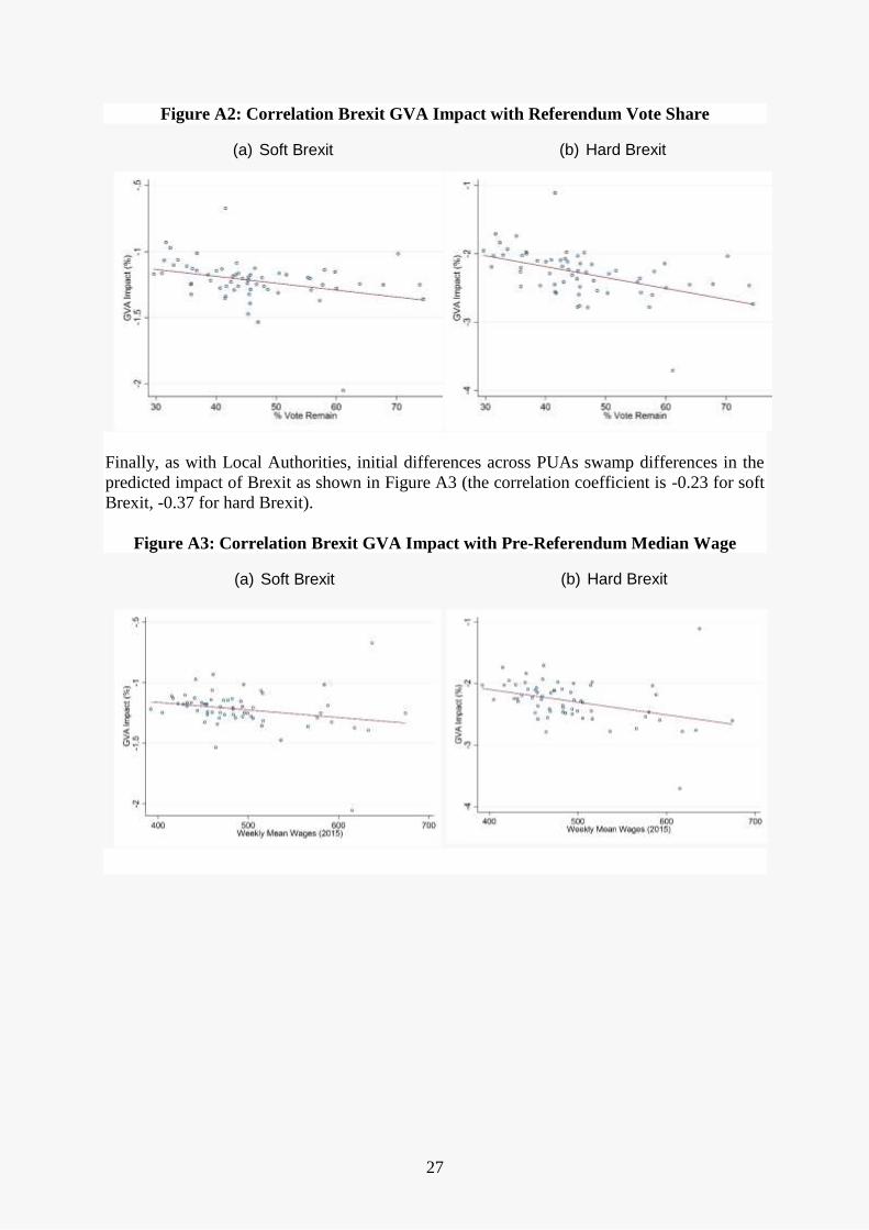
As for Local Authorities, Figure 2 shows that PUAs that are predicted to be most

negatively affected by Brexit were more likely to vote remain. As with Local Authorities, the

correlation is particularly striking for the predicted impacts under hard Brexit (the correlation coefficient is -0.33 for soft Brexit, -0.48 for hard Brexit).

27

Figure A2: Correlation Brexit GVA Impact with Referendum Vote Share

(a) Soft Brexit (b) Hard Brexit

Finally, as with Local Authorities, initial differences across PUAs swamp differences in the

predicted impact of Brexit as shown in Figure A3 (the correlation coefficient is -0.23 for soft

Brexit, -0.37 for hard Brexit).

Figure A3: Correlation Brexit GVA Impact with Pre-Referendum Median Wage

(a) Soft Brexit (b) Hard Brexit