the lindelof class of l-functions · chapter 1 introduction the riemann zeta-function is de ned on...
TRANSCRIPT

The Lindelof class of L-functions
by
Anup B Dixit
A thesis submitted in conformity with the requirementsfor the degree of Doctor of PhilosophyGraduate Department of Mathematics
University of Toronto
© Copyright 2018 by Anup B Dixit
Abstract
The Lindelof class of L-functions
Anup B Dixit
Doctor of Philosophy
Graduate Department of Mathematics
University of Toronto
2018
Meromorphic functions, called L-functions, play a vital role in number theory. In
1989, Selberg defined a class of L-functions that serves as an axiomatic model for L-
functions arising from geometry and arithmetic. Even though the Selberg class success-
fully captures many characteristics common to most L-functions, it fails to be closed
under addition. This creates obstructions, in particular, not allowing us to interpolate
between L-functions. To overcome this limitation, V. K. Murty defined a general class
of L-functions based on their growth rather than functional equation and Euler product.
This class, which is called the Lindelof class of L-functions, is endowed with the structure
of a ring.
In this thesis, we study further properties of this class, specifically, its ring structure
and topological structure. We also study the zero distribution and the a-value distribu-
tion of elements in this class and prove certain uniqueness results, showing that distinct
elements cannot share complex values and L-functions in this class cannot share two
distinct values with any other meromorphic function. We also establish the value dis-
tribution theory for this class with respect to the universality property, which states
that every holomorphic function is approximated infinitely often by vertical shifts of an
L-function. In this context, we precisely formulate and give some evidence towards the
Linnik-Ibragimov conjecture.
ii

To my parents.
iii

Acknowledgements
I extend my sincere gratitude to my mentor and advisor Prof. V. Kumar Murty not only
for his guidance, support and motivation through out my graduate studies but also for
many discussions outside mathematics, which have helped me develop as an individual
and shape my ideas and understanding.
I also thank my supervisory committee members Prof. Stephen Kudla and Prof.
Florian Herzig for their encouragement and insightful comments. My sincere thanks to
Prof. Arul Shankar and Prof. Jacob Tsimerman for many exciting discussions. I am
grateful to Prof. Steve Gonek for reading my thesis carefully, providing many helpful
suggestions and also for being my external committee member.
I am grateful to Prof. M. Ram Murty for his friendliness and support during my visit
to Queen’s University. I also thank Prof. Yu Ru Liu for inviting me to University of
Waterloo and making my trip a pleasant one.
I am grateful to Prof. Purusottam Rath and Prof. Sanoli Gun for their encouragement
and friendship during all my visits to India. I also thank Prof. Pramath Sastry for his
kindness and motivation through out these years.
I am deeply thankful to Ananth, Akshay, Gaurav, Abhishek, Siddhi, Padma, Payman
and Chia-Cheng for their friendship and making these years of graduate life enjoyable. I
specially thank Roni for his wonderful company and support outside the academic envi-
ronment. I also thank all the members of Ganita for providing a lively work environment
through out these years.
I thank all the staff members of the math department at University of Toronto,
especially Jemima, Patrina, Ashley and Sonja for their administrative help. My special
thanks to the late Ida Bulat, who helped me in settling down and dealing with many
unpleasant incidents during my first two years in Toronto.
I thank the Vedanta Society of Toronto for thoughtful discussions and teaching me
the virtue of introspection.
iv

I am most thankful to my parents, my sister, my brother-in-law and my childhood
friend Sukant for supporting me through out my ups and downs. My special thanks to
my father for introducing me to the charms of mathematics at a very early age, without
which I would not have reached at this stage.
v

Contents
1 Introduction 1
1.1 The Riemann zeta-function . . . . . . . . . . . . . . . . . . . . . . . . . 2
1.2 Organization of thesis . . . . . . . . . . . . . . . . . . . . . . . . . . . . . 5
2 The Selberg class 7
2.1 Examples . . . . . . . . . . . . . . . . . . . . . . . . . . . . . . . . . . . 9
2.2 The Generalized Riemann hypothesis . . . . . . . . . . . . . . . . . . . . 14
2.3 Selberg’s Conjectures . . . . . . . . . . . . . . . . . . . . . . . . . . . . . 15
2.4 The Lindelof Hypothesis . . . . . . . . . . . . . . . . . . . . . . . . . . . 22
3 The Lindelof class 27
3.1 The growth parameters . . . . . . . . . . . . . . . . . . . . . . . . . . . . 28
3.2 The invariants cF and c∗F . . . . . . . . . . . . . . . . . . . . . . . . . . . 32
3.3 The generalized Lindelof hypothesis . . . . . . . . . . . . . . . . . . . . . 45
3.4 The Lindelof class . . . . . . . . . . . . . . . . . . . . . . . . . . . . . . . 47
3.5 Ring theoretic properties of M, L and L∗ . . . . . . . . . . . . . . . . . . 48
3.5.1 Primitive elements in M and L∗ . . . . . . . . . . . . . . . . . . . 52
3.6 Ideals in L and L∗ . . . . . . . . . . . . . . . . . . . . . . . . . . . . . . 56
3.7 Topology on L and L∗ . . . . . . . . . . . . . . . . . . . . . . . . . . . . 58
4 Value Distribution and Uniqueness Theorems 61
vi

4.1 Number of zeroes . . . . . . . . . . . . . . . . . . . . . . . . . . . . . . . 62
4.2 The class M1 . . . . . . . . . . . . . . . . . . . . . . . . . . . . . . . . . 65
4.3 Uniqueness results . . . . . . . . . . . . . . . . . . . . . . . . . . . . . . 70
4.4 Nevanlinna Theory . . . . . . . . . . . . . . . . . . . . . . . . . . . . . . 71
4.5 Main Theorems . . . . . . . . . . . . . . . . . . . . . . . . . . . . . . . . 74
4.6 Proof of the theorems . . . . . . . . . . . . . . . . . . . . . . . . . . . . . 76
4.6.1 Proof of Theorem 4.5.1 . . . . . . . . . . . . . . . . . . . . . . . . 76
4.6.2 Proof of Theorem 4.5.2 . . . . . . . . . . . . . . . . . . . . . . . . 77
4.6.3 Proof of Theorem 4.5.3 . . . . . . . . . . . . . . . . . . . . . . . . 78
4.6.4 Proof of Theorem 4.5.4 . . . . . . . . . . . . . . . . . . . . . . . . 81
5 Universality and the Linnik-Ibragimov Conjecture 84
5.1 Voronin’s universality theorem . . . . . . . . . . . . . . . . . . . . . . . . 84
5.2 Linnik-Ibragimov conjecture . . . . . . . . . . . . . . . . . . . . . . . . . 90
5.3 Main results . . . . . . . . . . . . . . . . . . . . . . . . . . . . . . . . . . 91
5.4 Limit and Density Theorems . . . . . . . . . . . . . . . . . . . . . . . . . 93
5.5 Proof of the main theorems . . . . . . . . . . . . . . . . . . . . . . . . . 98
5.6 The Generalized Strong Recurrence . . . . . . . . . . . . . . . . . . . . . 102
Bibliography 105
vii

Chapter 1
Introduction
The Riemann zeta-function is defined on <(s) > 1 by
ζ(s) :=∞∑n=1
1
ns=∏
p prime
(1− 1
ps
)−1
. (1.1)
The Dirichlet series and the Euler product of the zeta-function converge absolutely on
the right half plane <(s) > 1 and uniformly on each compact set in this plane. Euler, who
studied ζ(s) as a function of a real variable was the first to notice this Euler product,
which can be regarded as the analytic version of the unique factorization of natural
numbers. Additionally, this product also captures information regarding the distribution
of primes in natural numbers. As Euler observed, the infinitude of primes follows from
the fact that the product diverges at s = 1. Riemann realized deeper connections between
the zeta-function and the distribution of prime numbers by studying ζ(s) as a function
of a complex variable. Earlier, Gauss had predicted that if π(x) denotes the number of
primes less than x, then asymptotically π(x) ∼ x/ log x. More precisely, he conjectured
that
π(x) ∼ Li(x) :=
∫ x
2
dt
log t
as x→∞.
1

Chapter 1. Introduction 2
In 1896, using ideas of Riemann, Jacques Hadamard and Charles Jean de la Vallee-
Poussin independently proved this conjecture, which is known today as the prime number
theorem. It turns out that this is a consequence of ζ(s) having a simple pole at s = 1
and being non-zero on the vertical line <(s) = 1.
This motivated a careful study of functions of the type (1.1). For instance, de la Vallee-
Poussin proved the prime number theorem for an arithmetic progression a (mod q), with
(a, q) = 1, using similar techniques by studying the function
L(s, χ) :=∞∑n=1
χ(n)
ns, (1.2)
where χ is a Dirichlet character modulo q, defined as a group homomorphism χ :
(Z/qZ)∗ → C∗ extended to χ : Z→ C by periodicity and setting χ(n) = 0 if (n, q) > 1.
Building on ideas of Riemann, connections were established between the zeroes of the
zeta-function and the distribution of prime numbers. In 1901, Helge von Koch observed
that the Riemann hypothesis implies a much stronger error term for the prime number
theorem.
In this thesis, we study functions similar to the zeta-function, which are called L-
functions. We introduce a class of L-functions and study their analytic properties, with
emphasis on the value distribution theory of such functions.
1.1 The Riemann zeta-function
In this section, we recall a few basic properties of the Riemann zeta-function ζ(s) and
motivate the definition of the Selberg class. The zeta-function given by
ζ(s) :=∞∑n=1
1
ns,
is absolutely convergent on <(s) > 1.

Chapter 1. Introduction 3
A series of the type∑
n an/ns is called a Dirichlet series. For any Dirichlet series
F (s) =∞∑n=1
anns,
the abscissa of absolute convergence, denoted as σ0(F ) is defined as the infimum of all
σ, such that the Dirichlet series is absolutely convergent on <(s) = σ. Similarly, we also
define the abscissa of convergence, denoted σc(F ) to be the infimum of all σ such that
the Dirichlet series is convergent for <(s) = σ. Moreover, we have that the series F (s)
is absolutely convergent for <(s) > σ0(F ) and convergent on <(s) > σc(F ) (see [45, pg.
289, sec. 9.11]).
The zeta-function has abscissa of absolute convergence and abscissa of convergence
given by σ0(ζ) = σc(ζ) = 1. Although, ζ(s) as a function in one complex variable was
introduced by Riemann, its special values at positive integers were already studied by
Euler.
For a real number x, let x denote the fractional part of x, i.e., x := x− [x]. By
partial summation, we obtain that for <(s) > 1,
ζ(s) =1
s− 1+
1
2+ s
∫ ∞1
12− xxs+1
dx. (1.3)
The integral in (1.3) is absolutely convergent for <(s) > 0 and uniformly convergent for
<(s) > ε for any ε > 0. Hence, (1.3) gives the analytic continuation of ζ(s) in the region
<(s) > 0 with a simple pole at s = 1 with residue 1.
Denote by Γ(s) the Euler gamma-function, which is defined for <(s) > 0 by
Γ(s) :=
∫ ∞0
e−xxs−1 dx.
Using the functional equation
Γ(s+ 1) = sΓ(s),

Chapter 1. Introduction 4
Γ(s) is meromorphically continuable to the whole of C except for simple poles at non-
positive integers s = 0,−1,−2, · · · , with residues given by
Ress=−nΓ(s) =(−1)n
n!.
This Euler gamma-function plays a crucial role in the functional equation of the zeta-
function, which enables us to meromorphically continue the zeta-function to C.
Consider the function
ξ(s) :=1
2s(s− 1)π−s/2Γ
(s
2
)ζ(s).
This is often referred to as the completed zeta-function. Riemann established the follow-
ing functional equation for ζ(s), given by
Proposition 1.1.1. ξ(s) = ξ(1− s).
In other words,
π−s/2Γ
(s
2
)ζ(s) = π−(1−s)/2Γ
(1− s
2
)ζ(1− s). (1.4)
This gives the analytic continuation of ζ(s) in the region <(s) < 1/2.
Since Γ(s) has poles at non-positive integers, using (1.4), we immediately conclude
that ζ(s) has simple zeroes at all negative even integers s = −2,−4,−6, · · · . These are
called the trivial zeroes of the zeta-function. Moreover, the Euler product
ζ(s) =∏p
(1− 1
ps
)−1
, for <(s) > 1
implies that ζ(s) does not have any zeroes in the region <(s) > 1. Now, using the
functional equation, we also conclude that ζ(s) has no zeroes other than the trivial
zeroes in the region <(s) < 0.

Chapter 1. Introduction 5
The strip 0 < <(s) < 1 is rather mysterious and the zeroes of ζ(s) in this region are
referred to as the non-trivial zeroes. Observing the symmetric nature of the functional
equation (1.4) of ζ(s), Riemann predicted that all the non-trivial zeroes of ζ(s) lie on the
vertical line <(s) = 1/2. This is known as the famous Riemann hypothesis.
Conjecture 1 (Riemann hypothesis). If ζ(s) = 0 for 0 < <(s) < 1, then <(s) = 1/2.
It is not very difficult to show that ζ(s) has no zeroes on the vertical line <(s) = 1.
This already results in the asymptotic formula for the number of primes less than x for
a large number x.
Similar approaches help us to prove the analogues of prime number theorem in differ-
ent settings. The prime number theorem in an arithmetic progression where the terms
are co-prime to the common difference is given by studying the Dirichlet L-functions.
In the number field setting, the analogue for the prime number theorem is given by
studying the Dedekind zeta-functions ζK(s). In each of these cases, the corresponding
“zeta” function, which is defined using some Euler product, captures the distribution of
primes in the respective underlying structure. There are further intricate connections
between primes and the zeroes of these functions. This raises the curiosity to study these
functions as a family and also better understand its zero-distribution.
1.2 Organization of thesis
Selberg initiated the study of a family of L-functions which satisfy the basic properties
of the Riemann zeta-function, called the Selberg class.
In chapter 2, we discuss some basic properties of the Selberg class. The emphasis of
this thesis is on the value distribution theory of L-functions. In chapter 2, we provide
some known results on the value distribution theory of L-functions in the Selberg class.
We also discuss Selberg’s orthogonality conjectures and some of its consequences.
In chapter 3, we introduce a larger family of L-functions, which overcomes some

Chapter 1. Introduction 6
limitations of the Selberg class. This new class M, based on the growth of L-functions
forms a ring and has a rather rich algebraic and geometric structure. It was defined by
V. K. Murty [34]. In particular, it forms a differential ring and has a natural topology
attached to it. We also study the ideal theory of this ring and show that it is non-
Noetherian. We address the analogous question to the degree conjecture in the context
of this new class and also provide the classification of elements with c∗F = 0. This chapter
forms a major part of [16], which is joint work with V. K. Murty.
In chapter 4, we study the a-value distribution of functions in the class M. We first
study the number of zeroes of L-functions in M, and give some upper and lower bounds
for the number of zeroes in a disc of radius r, centered at the origin. Using this and further
tools from Nevanlinna theory, we prove some uniqueness results. The main theorems in
this chapter are Theorem 4.5.1, 4.5.2, 4.5.3 and 4.5.4. They also appear in [14].
In chapter 5, we study the problem of universality of L-functions in M. The uni-
versality property of an L-function in a strip D vaguely claims that any holomorphic
function is approximated by infinitely many vertical shifts of the L-function in D. This
universality property is known for the elements in the Selberg class and also a number
of other naturally occurring L-functions. In view of this, Yu V. Linnik and I. A. Ibrag-
imov conjectured that all Dirichlet series with analytic continuation, satisfying certain
“growth conditions” must be universal in “some region”. In this context, we explicitly
characterize the growth condition for the L-function and describe the region where we
expect the function to be universal. Thus, we formulate the Linnik-Ibragimov conjecture
more explicitly and also provide partial results in this direction. Our main theorems in
this chapter are Theorem 5.3.1 and 5.3.2. These results will appear in [15].

Chapter 2
The Selberg class
In 1989, A. Selberg [40] defined a general class of L-functions having Euler product,
analytic continuation and functional equation of the similar type as the Riemann zeta-
function. He formulated some fundamental conjectures on the elements of this class.
Ever since, this class of L-functions has been extensively studied and these conjectures
have been known to have far reaching consequences.
Definition 2.0.1. The Selberg class S consists of meromorphic functions F (s) satisfying
the following properties.
1. Dirichlet series- It can be expressed as a Dirichlet series
F (s) =∞∑n=1
aF (n)
ns,
which is absolutely convergent in the region <(s) > 1. We also normalize the leading
coefficient as aF (1) = 1.
2. Analytic continuation - There exists a non-negative integer k, such that (s −
1)kF (s) is an entire function of finite order.
3. Functional equation - There exist real numbers Q > 0 and αi > 0, complex
7

Chapter 2. The Selberg class 8
numbers βi and w ∈ C, with Re(βi) ≥ 0 and |w| = 1, such that
Φ(s) := Qs∏i
Γ(αis+ βi)F (s) (2.1)
satisfies the functional equation
Φ(s) = wΦ(1− s).
4. Euler product - There is an Euler product of the form
F (s) =∏
p prime
Fp(s), (2.2)
where
logFp(s) =∞∑k=1
bpk
pks
with bpk = O(pkθ) for some θ < 1/2.
5. Ramanujan hypothesis - For any ε > 0,
|aF (n)| = Oε(nε). (2.3)
The Euler product implies that the coefficients aF (n) are multiplicative, i.e., aF (mn) =
aF (m)aF (n) when (m,n) = 1. Moreover, each Euler factor also has a Dirichlet series rep-
resentation
Fp(s) =∞∑k=0
aF (pk)
pks,
which is absolutely convergent on <(s) > 0 and non-vanishing on <(s) > θ, where θ is
as in (2.2).

Chapter 2. The Selberg class 9
2.1 Examples
1. The Riemann zeta-function ζ(s) ∈ S.
2. Dirichlet L-functions L(s, χ) and their vertical shifts L(s + iθ, χ) are in S, where
χ is a primitive Dirichlet character and θ ∈ R. Note that ζ(s + iθ) /∈ S for θ 6= 0,
since it has a pole at s = 1− iθ.
3. Dedekind zeta functions ζK(s) defined as
ζK(s) :=∑a⊆OK
1
(NK/Q(a))s,
where OK denotes the ring of integers of K and a runs over all ideals of OK , are
also elements of the Selberg class.
4. Let L/K be a Galois extension of number fields, with Galois group G. Let ρ : G→
GLn(C) be a representation of G. The associated Artin L-function is defined as
L(s, ρ, L/K) :=∏p∈K
det
(I − (Np)−sρ(σq)
∣∣V Iq
)−1
where q is a prime ideal in L lying over prime ideal p in K, σq is the Frobenius
automorphism associated to q and V Iq is the complex vector space fixed by the
inertia subgroup Iq.
A conjecture of Artin states that for non-trivial irreducible representation ρ of
Gal(L/K), the associated Artin L-function L(s, ρ, L/K) is entire. If the Artin
conjecture is true, then these functions lie in the Selberg class.
5. Let f be a holomorphic newform of weight k to some congruence subgroup Γ0(N).

Chapter 2. The Selberg class 10
Suppose its Fourier expansion is given by
f(z) =∞∑n=1
c(n) exp(2πinz).
Then, its normalized Dirichlet coefficients are given by
a(n) := c(n)n(1−k)/2,
and the associated L-function given by L(s) :=∑∞
n=1 a(n)/ns for <(s) > 1 is an
element in the Selberg class. It is also believed that the normalized L-function
associated to a non-holomorphic newforms is an element in the Selberg class, but
the Ramanujan hypothesis is yet to be proven in this case.
6. The L-function associated to the Rankin-Selberg convolution of any two holomor-
phic newforms is in the Selberg class.
The constants in the functional equation (2.1) depend on F , and although the func-
tional equation may not be unique, we have some well-defined invariants, such as the
degree dF of F , which is defined as
dF := 2∑i
αi.
The factor Q in the functional equation gives rise to another invariant referred to as the
conductor qF , which is defined as
qF := (2π)dFQ2∏i
αi2αi . (2.4)
It is an interesting conjecture that both the degree and the conductor for elements in
the Selberg class are non-negative integers.

Chapter 2. The Selberg class 11
Conjecture 2 (see Selberg [40], Conrey-Ghosh [12]). If F ∈ S, then dF and qF are
non-negative integers.
There is recent progress towards the degree conjecture. In 1993, it was shown by
Conrey-Ghosh [12] that for F (s) in the Selberg class, if dF < 1 then dF = 0. This was
proved using the fact that any non-trivial element in the Selberg class must satisfy a
certain growth condition, which is captured by the degree. We give the proof of this
statement here and shall use this idea to prove a more general statement in Chapter 3.
Theorem 2.1.1 (Conrey-Ghosh, 1992). If F (s) ∈ S, then F = 1 or dF ≥ 1.
Proof. Suppose dF < 1. It suffices to show that dF = 0, since the only element in S with
dF = 0 is the constant function F = 1. Let
F (s) =∞∑n=1
aF (n)
ns,
for <(s) > 1. Consider the function
f(x) :=∞∑n=1
aF (n)e−nx.
We know that∞∑n=1
aF (n)e−nx =1
2πi
∫(2)
F (s)Γ(s)x−sds,
where the integral is on the vertical line <(s) = 2. By the growth of F (s) and convexity
conditions due to Phragmen-Lindelof theorem, F (s) has a polynomial growth in |t| in
vertical strips. Thus, moving the line of integration to the left and taking into account
the possible pole at s = 1 of F (s) and poles of Γ(s) at s = 0,−1,−2, ..., we get that
f(x) =P (log x)
x+∞∑n=0
F (−n)
n!(−x)n,

Chapter 2. The Selberg class 12
where P is a polynomial. Let the functional equation for F be given by
ψ(s) := γF (s)F (s) = ψ(1− s).
Then, we have
∞∑n=0
F (−n)
n!(−x)n =
∞∑n=0
(−1)nγF (n+ 1)F (n+ 1)
γF (−n)n!xn,
which is an entire function in x since
γF (n+ 1)
γF (−n)n! n−(1−dF )nAn,
for some constant A > 0.
Hence, the function f(x) is analytic in C\x ≤ 0 : x ∈ R. But, this function is also
periodic with period 2πi and so it converges for all x. Thus, the function
f(z) =∞∑n=1
aF (n)e−nz
is entire. Taking z = −1, we get that
∞∑n=1
aF (n)en
is convergent and thus, aF (n) = o(e−n). So, the coefficients have exponential decay and
therefore, aF (n)nk 1 for all k ≥ 1. Hence, we have that
∞∑n=1
aF (n)
ns
is absolutely convergent for all values of s, and bounded on any right half plane. We

Chapter 2. The Selberg class 13
further notice that for <(s) = σ > 1
F (1− s) =ψ(s)
γ(1− s)∼ γ(s)
γ(1− s).
Using Stirlings formula, we get
∣∣∣∣ γ(s)
γ(1− s)
∣∣∣∣ ∼ c(σ)tdF (σ−1/2),
where c(σ) > 0 is a constant depending on σ. Since F (s) is bounded on any right half
plane, we get dF = 0 as required.
More recently, Perelli and Kaczorowski showed that for F (s) ∈ S, if 0 < dF < 2 then
dF = 1. In general, the degree conjecture is still open. But, a stronger version of this
conjecture is expected to be true.
Conjecture 3 (Stronger degree conjecture). For F (s) ∈ S, there exists a functional
equation of the form (2.1), where each αi = 1/2.
It is known due to Conrey and Ghosh [12] that the functions of degree one in the
Selberg class are the Riemann zeta-function ζ(s), Dirichlet L-functions L(s, χ) and their
shifts L(s + iθ, χ), where χ is non-principal primitive and θ ∈ R. For higher degrees,
there is no such classification so far.
However, there are known examples of elements in the Selberg class with higher
degrees. Dedekind zeta-functions attached to a number field K/Q denoted ζK(s) has
degree equal to the degree of the field extension [K : Q]. L-functions associated to
holomorphic newforms (see Example 5) have degree 2. Moreover, L-functions associated
to non-holomorphic newforms, if in the Selberg class, would also have degree 2. The
Rankin-Selberg L-function of normalized eigenforms are elements of the Selberg class of
degree 4.

Chapter 2. The Selberg class 14
Apart from the alternate interpretation of degree in terms of the growth of the func-
tion (as used in the proof above), there is another interpretation in terms of the zero-
distribution.
Let F (s) ∈ S. Define
N(T, F ) := # zeroes of F (s) in the region 0 < <(s) < 1 and |=(s)| < T.
We have the asymptotic formula of N(T, F ) in terms of the degree of F given by
N(T, F ) ∼ dFπT log T (2.5)
as T →∞. We will revisit this topic in Chapters 3 and 4.
2.2 The Generalized Riemann hypothesis
From the Euler-product (2.2) representation of F ∈ S, we conclude that F (s) has no
zeroes in the region <(s) > 1. Moreover, the functional equation (2.1) gives rise to
zeroes of F (s) corresponding to the poles of the Γ-factors. More precisely, we get that
all the zeroes in the region <(s) < 0 are given by
s = −m+ βjαj
,
for all non-negative integers m and αj, βj as in (2.1). These zeroes are called the trivial
zeroes of F (s). Thus, we have the notion of the critical strip 0 < <(s) < 1 where all
the other zeroes lie. These zeroes are called the non-trivial zeroes of F (s). Due to the
symmetric nature of the functional equation and the structure arising from the Euler
product discussed later, it is expected that elements in the Selberg class must satisfy the
analogue of the Riemann hypothesis.

Chapter 2. The Selberg class 15
Conjecture 4 (The Generalized Riemann hypothesis). There are no zeroes of F (s) ∈ S
in the region <(s) > 1/2.
Each axiom in the definition of the Selberg class is vital for expecting the Riemann
hypothesis to hold.
1. The Dirichlet series representation of F ∈ S must be of the form∑
n an/ns. We
do not include the generalized Dirichlet series given by F (s) =∑
n ane−λns in the
Selberg class. For instance, the Hurwitz zeta-function ζ(s, α) for α ∈ (0, 1) is not
a member of the Selberg class because it would violate the Riemann hypothesis.
2. The condition that F (s) ∈ S has a possible pole at s = 1 is necessary because we
expect the poles of F ∈ S to arise from the pole of the Riemann zeta-function.
Therefore, if F (s) has finitely many poles, we should be able to factorize it as
product of shifted Riemann-zeta functions to account for the poles at points other
than s = 1. For a ∈ C satisfying <(a) 6= 0, ζ(s+a) violates the Riemann hypothesis,
because we would then have infinitely many zeroes on <(s) = 1/2− a.
3. In the Euler product (2.2), the condition θ < 1/2 is important because we expect
the Euler factors to be convergent in the region <(s) > 0. For example, suppose
the Euler factor corresponding to the prime p = 2 is given by
F2(s) =
(1− 2
2s
)−1
=∞∑m=0
2m
2ms.
Here we have θ = 1 and clearly see that F2(s) has poles on <(s) = 1 and hence not
analytic on <(s) > 0.
2.3 Selberg’s Conjectures
The elements in the Selberg class are not closed under linear combination. But, the
Selberg class is closed under multiplication and forms a semi-group with respect to mul-

Chapter 2. The Selberg class 16
tiplication i.e., if F,G,H ∈ S, then FG ∈ S and F (GH) = (FG)H.
The fundamental elements with respect to multiplication in S are called the primitive
elements.
Definition 2.3.1. F ∈ S is said to be a primitive element if any factorization F = F1F2
with F1, F2 ∈ S implies that either F1 = 1 or F2 = 1.
In other words, an element in S is primitive if it cannot be further factorized into
non-trivial elements in S.
Using the characterization of degree in (2.5), we have that if F ∈ S has a factorization
F = F1F2, with F1, F2 ∈ S, then
N(T, F ) = N(T, F1) +N(T, F2).
Taking T →∞, we conclude that
dF = dF1 + dF2 .
We also know from Theorem 2.1.1 that non-trivial elements in S cannot have degree < 1.
Therefore, we cannot factorize an element F ∈ S indefinitely. So, every element in the
Selberg class can be factorized into primitive elements.
Proposition 2.3.2. Every element F ∈ S can be factorized into primitive elements in
S.
It is still unknown whether the above factorization is unique.
Conjecture 5 (Unique Factorization in S). Every element F ∈ S can be uniquely fac-
torized into primitive elements.
From the above discussion, it is clear that every element F ∈ S with degree dF = 1 is
a primitive element. Thus, the Riemann zeta-function and Dirichlet L-functions are all

Chapter 2. The Selberg class 17
primitive elements in the Selberg class. M. R. Murty [36] produced primitive elements
of degree 2 associated to holomorphic newforms.
Selberg’s conjectures claim that these distinct elements in S do not interact with each
other. In particular, the primitive elements are in some sense orthogonal to each other.
Conjecture 6 (Selberg’s conjectures). In [40], Selberg made the following conjectures.
1. Conjecture A - Let F ∈ S. There exists a constant nF such that
∑p≤x
|aF (p)|2
p= nF log log x+O(1). (2.6)
2. Conjecture B - Let F,G ∈ S be primitive elements. Then
∑p≤x
aF (p)aG(p)
p=
log log x+O(1), if F = G,
O(1) otherwise.
Conjecture B is known as the Selberg’s orthogonality conjecture.
It is easy to verify Conjecture A in particular cases. For instance, Conjecture A clearly
holds for the Riemann zeta-function. Moreover, using the prime number theorem for
arithmetic progression, one can verify Conjecture A for Dirichlet L-functions. Conjecture
B can also be verified in the case of Dirichlet L-functions using the orthogonality relations
for characters.
In the view of Proposition 2.3.2, it is easy to see that Conjecture B implies Conjecture
A. Let F ∈ S has a factorization into primitive elements given by
F (s) = F1(s)F2(s) · · ·Fm(s),

Chapter 2. The Selberg class 18
where Fk(s) is primitive for all 1 ≤ k ≤ m. Then, we have
∑p≤x
|aF (p)|2
p=
∑1≤j≤k≤m
∑p≤x
aFj(p)aFk(p)
p.
By Conjecture B, the above sum is of the form
m log log x+O(1),
where m is the number of factors in the factorization of F (s) into primitive elements.
Selberg [40] noted that there are connections between these conjectures and several
other conjectures like the Sato-Tate conjecture, Langlands conjectures etc. Conrey and
Ghosh [12] showed that Conjecture B implies the unique factorization into primitives in
S as shown in the proposition below. In [37], M.R. Murty proved that Conjecture B
implies the strong Artin’s conjecture. More precisely, he showed that for any irreducible
representation ρ of Gal(L/K) of degree n, there exists an irreducible cuspidal automor-
phic representation π of GLn(AQ), such that L(s, ρ, L/K) = L(s, π). Since L(s, π) are
known to be entire, so is L(s, ρ, L/K).
Proposition 2.3.3. Conjecture B implies that every element F ∈ S has unique factor-
ization into primitive elements.
Proof. Suppose F ∈ S has two different factorizations into primitives, say,
F (s) =m∏j=1
Fj(s) =r∏
k=1
Gk(s).
We can further assume that no Fj is same as Gk. Since
m∑j=1
aFj(p) =r∑
k=1
aGk(p),

Chapter 2. The Selberg class 19
multiplying both sides by aF1(p)/p and summing over p ≤ x, we get
m∑j=1
∑p≤x
aFj(p)aF1(p)
p=
r∑k=1
∑p≤x
aGk(p)aF1(p)
p. (2.7)
Now, Conjecture B implies that the LHS of (2.7) is unbounded where as the RHS is
bounded as x tends to infinity, which leads to a contradiction.
By a similar argument as above, we also conclude the following.
Proposition 2.3.4. An element F ∈ S is a primitive element if and only if nF = 1,
where nF is given by (2.6).
The Selberg class is designed to model the class of L-functions satisfying the Riemann
hypothesis. So, one might ask whether the analogue of prime number theorem is true
for the elements in the Selberg class. Recall that the prime number theorem for natural
numbers follows from the fact that ζ(s) does not vanish on the vertical line <(s) = 1.
So, the following statement can be considered as the analogue to prime number theorem
in the Selberg class.
Conjecture 7 (Generalized prime number theorem). If F ∈ S, then F (s) 6= 0 for
s = 1 + it for any t ∈ R.
Unfortunately, this is still open. Recently, Kaczorowski and Perelli [24] proposed
a refined version of the prime number theorem for the Selberg class. But, the above
conjecture can be shown assuming the Conjecture B.
Proposition 2.3.5. Conjecture B implies Conjecture 7.
Proof. We use the following lemmas.
Lemma 2.3.6. If F ∈ S has a pole or a zero at s = 1 + iθ for θ ∈ R, then
∑p≤x
app1+iθ

Chapter 2. The Selberg class 20
is unbounded as x tends to ∞.
Proof. If F (s) has a pole or zero of order m 6= 0 at 1 + iθ, then we have
F (s) ∼ c(s− (1 + iθ))m,
near 1 + iθ. Writing s = σ + it and taking log, we get
logF (s) ∼ m log(σ − 1)
near s = 1 + iθ. Moreover, from the Euler product, we have for σ > 1,
logF (s) =∑p
aF (p)
ps+O(1).
Thus, we get ∑p
aF (p)
ps∼ m log(σ − 1),
as σ → 1+. Assume the function
S(x) =∑p≤x
aF (p)
p1+iθ
is bounded. Then, we have
∑p
aF (p)
ps=
∫ ∞1
x1−σdS(x)
= (σ − 1)
∫ ∞1
S(x)x−σ dx 1,
which is a contradiction.
There are many more interesting consequences of the orthogonality Conjecture B.
Using a similar argument as in Proposition 2.3.3, one can prove that the Conjecture B

Chapter 2. The Selberg class 21
implies that if F ∈ S has a pole at s = 1, it must be coming the Riemann-zeta function.
More precisely,
Lemma 2.3.7. If F (s) ∈ S has a pole of order m at s = 1, then Conjecture B implies
that F (s) = ζ(s)mL(s), where L ∈ S.
Proof. Since Conjecture B implies unique factorization into primitive elements in S, it
suffices to show that if F ∈ S is a primitive element with a pole at s = 1, then it is ζ(s).
From Proposition 2.3.4 we know that nζ = 1 and nF = 1. If F 6= ζ, then Conjecture B
implies that ∑p≤x
aF (p)
p 1,
which is a contradiction.
This expectation that every pole comes from ζ(s) can be thought of as the amelio-
ration of Dedekind’s conjecture, which states that every Dedekind zeta-function ζK(s)
must factorize through ζ(s).
Now, we are ready to prove the proposition. Since Conjecture B implies unique
factorization, it is enough to show the non-vanishing of F (s) on <(s) = 1 for primitive
elements F ∈ S. Since ζ(s) does not vanish on <(s) = 1, using Lemma 2.3.7, we can
further assume that F (s) is entire. This implies that F (s+ iα) ∈ S for any α ∈ R.
Now, if F has a zero at s = 1 + iθ, Lemma 2.3.6 implies that
∑p≤x
aF (p)
p1+iθ
is unbounded as x→∞. But the Conjecture B applied to ζ(s) and F (s+ iθ) yields
∑p≤x
aF (p)
p1+iθ 1,
which leads to a contradiction.

Chapter 2. The Selberg class 22
In [24], Kaczorowski and Perelli proved the Conjecture 7 with an assumption weaker
than Conjecture A. This weaker assumption is often called the Normality conjecture,
which is similar to the Conjecture A, but with a weaker error term.
2.4 The Lindelof Hypothesis
We say that a function F (s), analytic in the strip σ1 ≤ <(s) ≤ σ2 with finitely many
poles in this region, is of finite order in this strip, if there exists a constant c > 0 such
that
F (s) |t|c as t→∞.
This order is different from the usual complex Ritt order (see Steuding [43, p.36]). One
can make similar definition of finite order in a right half plane, say <(s) > σ1. Any
Dirichlet series is of finite order in its half-plane of convergence (conditional convergence).
The order of growth of meromorphic function is an important theme. As we shall
see, any Dirichlet series satisfying a Riemann type functional equation is of finite order
in any half-plane <(s) > σ for any σ ∈ R. First, we make the following definition.
Definition 2.4.1. Let F (s) ∈ S. Define
µF (σ) := lim sup|t|→∞
log |F (σ + it)|log |t|
.
Since F (s) is absolutely convergent on <(s) > 1, we immediately obtain that F (s) is
bounded in the region <(s) > 1 + ε for any ε > 0. Hence, µF (σ) = 0 for σ > 1 + ε. The
order of growth in the left half plane <(s) < 0 is obtained using the functional equation
F (s) =γ(1− s)γ(s)
F (1− s),

Chapter 2. The Selberg class 23
where the gamma-factor is given by
γ(s) = Qs
k∏j=1
Γ(αjs+ βj).
Applying Stirling’s formula, we get for t ≥ 1, uniformly in σ,
γ(1− s)γ(s)
=
(αQ2tdF
)1/2−σ−it
exp
(itdF +
iπ(β − dF )
4
)(ω +O
(1
T
)), (2.8)
where
α :=k∏j=1
α2αjj and β := 2
k∑j=1
(1− 2βj).
Recall the Phragmen-Lindelof theorem given by
Theorem 2.4.2 (Phragmen-Lindelof). Let f(s) be analytic in the strip σ1 ≤ <(s) ≤ σ2
with f(s) exp (ε|t|). If
|f(σ1 + it)| |t|c1 and
|f(σ2 + it)| |t|c2 ,
then
|f(σ + it)| |t|c(σ),
uniformly in σ1 ≤ σ ≤ σ2, where c(σ) is linear in σ with c(σ1) = c1 and c(σ2) = c2.
Using the Phragmen-Lindelof theorem and (2.8), we get the following upper bounds
on the growth of an element in S.
Theorem 2.4.3. Let F ∈ S. Uniformly in σ, as |t| → ∞,
F (σ + it) ∼ |t|(1/2−σ)dF |F (1− σ + it)|.

Chapter 2. The Selberg class 24
We also have
µF (σ) ≤
0 if σ > 1,
12dF (1− σ) if 0 ≤ σ ≤ 1,
dF (12− σ) if σ < 0.
Lindelof conjectured that the order of growth of the Riemann zeta-function is much
smaller than what the Phragmen-Lindelof theorem gives. In fact, he conjectured that
ζ(s) is bounded on σ > 1/2. This statement is known to be false. But, a weaker version
would state that µζ(1/2) = 0. In other words,
∣∣∣∣ζ(1
2+ it
)∣∣∣∣ |t|ε,for any ε > 0. This is known as the Lindelof hypothesis. Note that, the Phragmen-
Lindelof theorem only implies that |ζ(1/2 + it)| ε |t|1/4+ε for any ε > 0. Any improve-
ment on the constant 1/4 is called the phenomena of “breaking convexity”. The best
known improvement on this constant is replacing 1/4 with 9/56. This is due to Bombieri
and Iwaniec [7] using Weyl’s method of estimating exponential sums, which was earlier
incorporated by Hardy and Littlewood to attack the same problem.
A more general statement of the Lindelof hypothesis on the Selberg class is given by
Conjecture 8 (Generalized Lindelof hypothesis). For F ∈ S and any ε > 0,
∣∣∣∣F(1
2+ it
)∣∣∣∣ |t|ε.It is known due to Littlewood that the Riemann hypothesis implies the Lindelof
hypothesis. Further, Conrey and Ghosh [13] showed that the Generalized Riemann hy-
pothesis implies the Generalized Lindelof hypothesis. They also computed the implied
constant in terms of the invariants arising from the functional equation of F (s). Moreover,
the Lindelof hypothesis itself has many interesting consequences. The most prominent
one is in the context of value distribution of L-functions.

Chapter 2. The Selberg class 25
For F ∈ S, let NF (σ, T ) denote the number of zeroes of F (s) in the region
s ∈ C : <(s) > σ, |=(s)| < T
.
The Lindelof hypothesis for Riemann zeta-function implies the density hypothesis,
which states that for σ > 1/2,
Nζ(σ, T ) T 2(1−σ).
In case of the Selberg class, the generalized Lindelof hypothesis implies a statement
regarding the zero-distribution of L-functions, which we call the zero hypothesis.
The classical result on zero density estimate due to Bohr and Landau [6] states that
most of the zeroes of ζ(s) are clustered near the 1/2-line, i.e., they showed that
Nζ(σ, T ) T 4σ(1−σ)+ε, (2.9)
for σ > 1/2.
More recently, we have the following density theorem due to Perelli and Kaczorowski
[24] for the Selberg class.
Theorem 2.4.4 (Density Theorem). For F ∈ S,
NF (σ, T )ε Tc(1−σ)+ε,
for σ > 1/2 and c = 4dF + 12.
The above zero-density estimate suggests that the number of zeroes close to the
vertical line <(s) = 1 is very small. In general, we formulate the zero hypothesis, which
claims that for F ∈ S all the zeroes are clustered near the 1/2-line.
Conjecture 9 (Zero Hypothesis). For F ∈ S, there is a positive constant c such that for

Chapter 2. The Selberg class 26
σ > 1/2,
NF (σ, T ) T 1−c(σ−1/2)+ε.

Chapter 3
The Lindelof class
The Selberg class, as described in Chapter 2, comprises of a general class of L-functions
satisfying axioms, which are expected of functions similar to the Riemann zeta-function.
Despite its generality, the Selberg class S has several limitations. For instance, it is not
closed under addition. This is due to the rigidity of the functional equation and the Euler
product, which are crucial in the definition of S. The functional equation provides some
satisfactory answers to the value distribution, in particular the zero distribution of L-
functions. In [8], Bombieri and Hejhal studied the zero distribution of linear combination
of L-functions in S, each having the same functional equation. However, in general a linear
combination of L-functions may not satisfy a functional equation. Thus, the question of
their value distribution, which is of significance, is not answered by studying the Selberg
class.
Moreover, some naturally occurring L-functions such as the Epstein zeta-function,
do not always have an Euler product and hence are not members of the Selberg class.
This raises the question of studying a larger class of L-functions, which would contain
linear combinations of known L-functions, i.e., one that is closed under addition and also
includes some naturally occurring L-functions, which are not part of the Selberg class.
This motivated V. Kumar Murty [34] to introduce a class of L-functions defined based
27

Chapter 3. The Lindelof class 28
on growth conditions. As we shall see in Chapter 4 and 5, this larger class of L-functions
seems to successfully find common patterns in its value distribution as in the case of the
Selberg class. Additionally, this class of L-functions also has a richer algebraic structure.
In the following section, we carefully define some growth parameters and introduce a
class of L-functions namely the class M.
3.1 The growth parameters
Definition 3.1.1. The class T. Define the class T to be the set of functions F (s)
satisfying the following conditions.
1. Dirichlet series - For σ > 1, F (s) is given by the absolutely convergent Dirichlet
series
F (s) =∞∑n=1
aF (n)
ns.
2. Analytic continuation - There exists a non-negative integer k, such that (s −
1)kF (s) is an entire function of order ≤ 1.
3. Ramanujan hypothesis - |aF (n)| = Oε(nε) for any ε > 0.
For the class T, we define growth parameters µ and µ∗, which would be analogous to
the definition of µF in 2.4.1 of Chapter 2.
Definition 3.1.2. Let F ∈ T be entire. Define µF (σ) as
µF (σ) :=
inf
λ ∈ R : |F (s)| ≤ (|s|+ 2)λ, for all s with Re(s) = σ
,
∞, if the infimum does not exist.
(3.1)

Chapter 3. The Lindelof class 29
Also define:
µ∗F (σ) :=
inf
λ ∈ R : |F (σ + it)| σ (|t|+ 2)λ
,
∞, if the infimum does not exist.
(3.2)
In the definition of µ∗F (σ), the implied constant depends on both F and σ, whereas
in µF (σ), the constant only depends on F and is independent of σ.
We further extend the definition of µF and µ∗F to all the elements in the class T as
follows.
Suppose F ∈ T has a pole of order k at s = 1. Consider the function
G(s) :=
(1− 2
2s
)kF (s). (3.3)
Clearly, G(s) is an entire function and belongs to T. We define
µF (σ) := µG(σ),
µ∗F (σ) := µ∗G(σ).
Intuitively, µ∗F (σ) does not see how F (s) behaves close to the real axis. It is only
dependent on the growth of F (s) on <(s) = σ and =(s) T for arbitrary large T . On
the other hand, µF (σ) captures an absolute bound for F (s) on the entire vertical line
<(s) = σ.
It follows from the definition that
µ∗F (σ) ≤ µF (σ)
for any σ. From the above definition, we immediately conclude the following.

Chapter 3. The Lindelof class 30
Proposition 3.1.3. Let F ∈ T. For σ > 1 + ε,
µ∗F (σ) = 0
µF (σ)F,ε 1.
for any ε > 0.
Proof. Since F ∈ T, it is given by a Dirichlet series F (s) =∑
n an/ns, which is absolutely
convergent for σ > 1 and hence bounded in the region σ ≥ 1+ε, with the bound depending
on F and ε, but independent of σ. Hence, we have the proposition.
Note that µF (σ) and µ∗F (σ) are always non-negative for all σ. This is because µ∗F (σ) =
0 for σ > 1. Hence, if µF (σ1) < 0, then by Phragmen-Lindelof theorem, µF (σ) ≤ 0 in the
strip σ1 ≤ <(s) ≤ σ. Thus, we get a vertical strip where F (s) is bounded and tends to
0 as =(s) → ∞. This is a contradiction. By a similar argument, we also conclude that
µF (σ) is always non-negative.
If F ∈ S, by the functional equation (2.1), using Stirling’s formula, we have (see [34],
Sec.2.1])
µ∗F (σ) ≤ 1
2dF (1− 2σ) for σ < 0. (3.4)
Using the Phragmen-Lindelof theorem, we deduce that
µ∗F (σ) ≤ 1
2dF (1− σ) for 0 < σ < 1.
The same results hold for µF up to a constant depending on F . To see this, we use
the functional equation for F ,
F (s) = ∆F (s)F (1− s),

Chapter 3. The Lindelof class 31
where
∆F (s) := ωQ1−2s
k∏j=1
Γ(αj(1− s) + βj)
Γ(αjs+ βj).
Using Stirling’s formula, we get
Lemma 3.1.4. For F ∈ S and t ≥ 1, uniformly in σ,
∆F (σ + it) =
(αQ2tdF
)1/2−σ−it
exp
(itdF +
iπ(β − dF )
4
)(ω +O
(1
T
)),
where
α :=k∏j=1
α2αjj and β := 2
k∑j=1
(1− 2βj).
By Lemma 3.1.4, we conclude that
µF (σ) ≤ 1
2dF (1− 2σ) +O(1) for σ < 0. (3.5)
and
µF (σ) ≤ 1
2dF (1− σ) +O(1) for 0 < σ < 1.
Thus, for F ∈ S, these parameters µF (σ) and µ∗F (σ) are well-defined (i.e., µF (σ), µ∗F (σ) <
∞). We imitate this behaviour of µ and µ∗ to introduce a growth condition. This leads
to the definition of class M.
Definition 3.1.5. The class M. Define the class M (see [34, sec.2.4]) to be the set of
functions F (s) satisfying the following conditions.
1. Dirichlet series - F (s) is given by a Dirichlet series
∞∑n=1
aF (n)
ns,
which is absolutely convergent in the right half plane <(s) > 1.

Chapter 3. The Lindelof class 32
2. Analytic continuation - There exists a non-negative integer k such that (s −
1)kF (s) is an entire function of order ≤ 1.
3. Growth condition - The quantity µF (σ)(1−2σ)
is bounded for σ < 0.
4. Ramanujan hypothesis - |aF (n)| = Oε(nε) for any ε > 0.
Notice that in the condition of analytic continuation, we have to force the complex
order to be≤ 1. In case of the Selberg class, this condition is implicit due to the functional
equation.
3.2 The invariants cF and c∗F
From the observation (3.4) and (3.5), we define the following invariants for M, which
would be considered analogous to the notion of degree in S.
Definition 3.2.1. For F ∈M, define
cF := lim supσ<0
2µF (σ)
1− 2σ,
c∗F := lim supσ<0
2µ∗F (σ)
1− 2σ.
By the growth condition, cF and c∗F are well-defined in M. Moreover, since µ∗F (σ) ≤
µF (σ) for all <(s) = σ, we have
c∗F ≤ cF .
Note that cF and c∗F are ≥ 0. Using the Phragmen-Lindelof theorem, we have
µF (σ) ≤ 1
2cF (1− σ),
µ∗F (σ) ≤ 1
2c∗F (1− σ)
for 0 < σ < 1. We mention a few examples.

Chapter 3. The Lindelof class 33
Proposition 3.2.2. Any Dirichlet polynomial F belongs to M and cF = c∗F = 0.
Proof. Suppose
F (s) =m∑n=1
anns.
Let s = σ + it. We can write
F (s) = a1 + 2−σa22−it + 3−σa33−it + ...+m−σamm−it.
Therefore, for some large k, there exists a constant M > 0, such that
|F (s)| ≤Mm−σ,
when σ < −k. By changing the base, we have
Mm−σ = M(|σ|+ 2)|σ| log(|σ|+2)m,
for σ < −k. By (3.1), we get
µF (σ) ≤ |σ| log(|σ|+2) m.
Therefore, we conclude,
lim supσ<0
µF (σ)
1− 2σ= 0.
Hence, cF = 0 which implies c∗F = 0.
Proposition 3.2.3. Any Dirichlet series F which is absolutely convergent on the whole
complex plane has c∗F = 0.
Proof. By (3.2), we can conclude that if a Dirichlet series F is absolutely convergent
on the vertical line <(s) = σ, then µ∗F (σ) = 0. Since, µ∗F (σ) = 0 for all σ, we have
c∗F = 0.
Chapter 3. The Lindelof class 34
Proposition 3.2.4. The Riemann zeta-function ζ(s) is in M and cζ = c∗ζ = 1.
Proposition 3.2.5. If F is an element in the Selberg class, then F also belongs to M.
Moreover, cF = c∗F and is given by the degree of F .
The proof of Proposition 3.2.4 and 3.2.5 will follow from Proposition 3.2.13.
Proposition 3.2.6. Linear combinations of elements in the Selberg class S are in M.
We shall see this later, when we prove that M forms a ring.
Another example of L-functions in M, which are not constructed from linear com-
bination of elements in S are the translates of Epstein zeta-functions. For a given real
positive definite n× n-matrix T , the Epstein zeta-function is defined as (see [17], [18])
ζ(T, s) :=∑
06=v∈Zn(vtTv)−s.
This series is absolutely convergent for <(s) > n/2. It can be analytically continued to
C except for a simple pole at s = n/2 with residue
πn/2
Γ(n/2)√
detT.
Moreover, it satisfies a functional equation. Let
ψ(T, s) := π−s/2Γ(s)ζ(T, s).
Then,
ψ(T, s) = (detT )−1/2ψ
(T−1,
n
2− s).
Thus, the function ζ(T, s+n/2−1) is an element in M. The growth condition is satisfied
because of the functional equation and further we have cζ(T,s+n/2−1) = c∗ζ(T,s+n/2−1) = 2.
Proposition 3.2.7. If F (s) belongs to M, then all its translates given by F (s) + a also
belong to M. Moreover, they have the same values of cF and c∗F .

Chapter 3. The Lindelof class 35
In order to ensure that M is closed under addition, we need to establish that these
invariants cF and c∗F in fact satisy an ultrametric inequality.
Proposition 3.2.8 ([34], Prop. 1). For F,G ∈M,
cFG ≤ cF + cG and cF+G ≤ max(cF , cG).
Similarly,
c∗FG ≤ c∗F + c∗G and c∗F+G ≤ max(c∗F , c∗G).
In fact, if cF > cG (resp. c∗F > c∗G), then
cF+G = cF (resp. c∗F+G = c∗F ).
Proof. The proof follows immediately from the definition of µF and µ∗F . This is because,
for any fixed σ and |t| > 1, we have
|F (σ + it)| σ |t|µ∗F (σ)+ε,
for any ε > 0. Therefore, for any F,G ∈M, we have
|FG(σ + it)| σ |t|µ∗F (σ)+µ∗G(σ)+ε.
Similarly,
|(F +G)(σ + it)| σ |t|µ∗F (σ) + |t|µ∗G(σ)+ε
σ |t|max (µ∗F (σ), µ∗G(σ))+ε.
Incorporating this into the definition of c∗F , we are done. Proof of the ultra-metric
inequalities for cF follows from a similar argument by replacing µ∗F with µF .

Chapter 3. The Lindelof class 36
As mentioned in the Example 4 above, for F ∈ S, cF and c∗F coincide with the degree
dF of F . Since dFG = dF + dG, we immediately get for F,G ∈ S,
cFG = cF + cG,
c∗FG = c∗F + c∗G.
The degree conjecture, as described in Conjecture 2 of Chapter 2, claims that the
degree of any element in S must be a non-negative integer. The question arises if we
can make similar claims about these invariants cF and c∗F . As it turns out, cF can take
non-integer values, in fact one can manufacture functions in M with any arbitrary non-
negative value of cF . But, we expect the analogue of the degree conjecture to be true for
the invariant c∗F .
Conjecture 10. Let F ∈M, then c∗F is always a non-negative integer.
In this direction imitating the argument of Conrey-Ghosh [12], in which they showed
that the degree dF in the Selberg class cannot take non-integer values between 0 and 1,
we get the following result.
Proposition 3.2.9 (Corrected version of [34], Prop. 3). Suppose F ∈ M. Then cF < 1
implies c∗F = 0.
Proof. Let F ∈M. For σ > 1, let F (s) =∑∞
n=1aF (n)ns
. Then we know that,
f(x) :=∞∑n=1
aF (n)e−nx =1
2πi
∫(2)
F (s)Γ(s)x−sds,
where the integration is on the line <(s) = 2.
By the growth condition and convexity, F has a polynomial growth in |t| in vertical
strips. Thus, moving the line of integration to the left and taking into account the
Chapter 3. The Lindelof class 37
possible pole at s = 1 of F (s) and poles of Γ(s) at s = 0,−1,−2, · · · , we get that
f(x) =P (log x)
x+∞∑n=0
F (−n)
n!(−x)n, (3.6)
where P is a polynomial. By the definition of cF , we have
|F (−n)| n12cF (1+2n)+ε.
Using Stirling’s formula, i.e,
n! ∼ nn−1/2e−n(2π)−1/2,
we get ∣∣∣∣F (−n)
n!(−x)n
∣∣∣∣ ncF+1
2+ε
(e|x|ncFn
)n.
If cF < 1, then the series in equation (3.6) converges absolutely for all values of x.
Hence, the function f(x) is analytic in C\x ≤ 0 : x ∈ R. But, this function is also
periodic with period 2πi and so it converges for all x. Thus, the function
f(z) =∞∑n=1
aF (n)e−nz
is entire. Taking z = −1, we get that
∞∑n=1
aF (n)en
is convergent and thus, aF (n) = o(e−n). So, the coefficients have exponential decay and
therefore, aF (n)nk 1 for all k ≥ 1. Hence, we have that
∞∑n=1
aF (n)
ns

Chapter 3. The Lindelof class 38
is absolutely convergent for all values of s. Therefore, µ∗F (σ) = 0 for all σ and hence
c∗F = 0.
We can completely characterize all F ∈ M such that c∗F = 0. These are precisely all
the functions, which when multiplied by a suitable Dirichlet polynomial gives a Dirichlet
series which is convergent on the whole complex plane. We invoke the following theorem
of Landau to prove the result.
Theorem 3.2.10 (Landau, [20] Chapter VII, sec. 10, Thm. 51). Let F (s) be an entire
function. Suppose F (s) has a Dirichlet series representation
F (s) =∞∑n=1
anns,
which is absolutely convergent for <(s) > 1. Also, suppose that
an = O(nε)
for all positive ε. If
F (s) = O(|t|β) (β > 0)
uniformly in the half plane <(s) > η, then the Dirichlet series is convergent in the half
plane <(s) > η1, where
η1 =
η+β1+β
, if η + β > 0
η + β, if η + β < 0.
Using the above Theorem 3.2.10, we get the following result classifying all elements
in M with c∗F = 0.
Proposition 3.2.11. Suppose F ∈M and let
H(s) = 1− 2
2s.

Chapter 3. The Lindelof class 39
If c∗F = 0, then the Dirichlet series given by
H(s)kF (s) =∞∑n=1
bnns,
is absolutely convergent on the whole complex plane, where k is the order of the possible
pole of F (s) at s = 1.
Proof. Let F ∈M. Suppose σ0(F ) is the abscissa of absolute convergence for the Dirichlet
series associated with F . If the Dirichlet series is not convergent on the whole complex
plane, then we have σ0(F ) > −∞. Note that
G(s) := F (s+ σ0(F )− 1)
is in M whose abscissa of absolute convergence is σ0(G) = 1. Therefore, without loss
of generality we assume that the Dirichlet series F (s) =∑∞
n=1 an/ns has abscissa of
absolute convergence σ0(F ) = 1.
Since c∗F = 0, we can choose a σ1 < 0 such that
F (σ1 + it) = O((|t|+ 2)ε(1/2−σ1)),
for any ε > 0. Using the Phragmen-Lindelof theorem, we get
F (σ + it) = O((|t|+ 2)ε(1/2−σ)) (3.7)
for σ1 < σ < 1. Let σ be fixed. For any ε1 > 0, choose ε = 2ε1(1−2σ)
in (3.7) to get
|F (σ + it)| = O((|t|+ 2)ε1).

Chapter 3. The Lindelof class 40
Suppose F (s) has a pole of order k at s = 1. Define
G(s) :=
(1− 2
2s
)kF (s).
G(s) is analytic on the whole complex plane and G ∈ M with the Dirichlet series repre-
sentation
G(s) =∞∑n=1
bnns
with abscissa of absolute convergence at σ0(G) = 1. Also c∗G = c∗F = 0 by the definition
of µ∗F .
Moreover, for σ1 0 and any ε > 0, we have
|G(σ + it)| = O((|t|)ε)
uniformly for σ > σ1. By Theorem 3.2.10, we conclude that the Dirichlet series repre-
sentation of
G(s) =∞∑n=1
bnns
converges in the half plane <(s) > σ1 +ε. Therefore, the abscissa of absolute convergence
is σ0(G) < σ1 + 1 + ε < 1, which contradicts the assumption that σ0 = 1.
Hence σ0(G) = −∞ and the Dirichlet series representation of
G(s) =∞∑n=1
bnns
is convergent on the whole complex plane and the proposition follows.
Next, we show that the analogue of the degree conjecture given by Conjecture 10
holds between 0 and 1, i.e., c∗F does not take non-integer values between 0 and 1.
Proposition 3.2.12. Suppose F (s) ∈M. Then c∗F < 1 implies c∗F = 0.

Chapter 3. The Lindelof class 41
Proof. Let c∗F < 1. Without loss of generality, we assume
F (s) =∞∑n=1
anns
has abscissa of absolute convergence σ0(F ) = 1. If F has a pole of order k at s = 1, we
consider
G(s) :=
(1− 2
2s
)kF (s).
As discussed in the proof of Proposition 3.2.11,
G(s) =∞∑n=1
bnns
also has abscissa of absolute convergence at σ0(G) = 1. Moreover, c∗G = c∗F .
Hence, for any ε > 0, we have a σ1 < 0, such that
|G(σ1 + it)| = O((|t|+ 2)c∗F (1/2−σ1)+ε).
Using Phragmen-Lindelof theorem on the strip σ1 < <(s) < 1, we get
|G(σ + it)| = O((|t|+ 2)c∗F (1/2−σ)+ε) (3.8)
for σ > σ1. By Theorem 3.2.10, we conclude that the Dirichlet series of G(s) converges
in the half plane <(s) > σ + c∗F (12− σ) + ε1 for any σ < 0 and ε1 > 0. Since c∗F < 1,
choosing σ 0 such that σ − c∗Fσ < −1, we get the convergence of the Dirichlet series
of G(s) on the half plane
<(s) > −1 +1
2c∗F .
Therefore, the Dirichlet series converges on <(s) > −12. Since the abscissa of absolute
convergence for the Dirichlet series of G(s) is σ0(G) = 1, we know that the abscissa of
convergence σc(G) ≥ 0, which leads to a contradiction.
Chapter 3. The Lindelof class 42
We finally show that these invariants cF and c∗F in fact coincide with the degree of
the Selberg class.
Proposition 3.2.13. Let F ∈ M, and suppose that F has a functional equation of the
Riemann type as in the Selberg class. Then cF = dF , where dF is the degree of F in the
sense of the Selberg class.
Proof. For simplicity, assume F has only one Γ-factor. We have
QsΓ(as+ b)F (s) = wQ1−sΓ(a(1− s) + b)F (1− s),
where a,Q are non-negative real numbers, b ∈ C with <(b) ≥ 0 and |w| = 1. We know
from (3.4) that cF ≤ dF . So we only need to show that cF is at least dF . We shall
first show it for the Riemann zeta-function and use this template to prove it in general.
Substituting s = 1− 2k for any integer k > 0 in the functional equation for ζ(s) gives
π−(1−2k)/2ζ(1− 2k)Γ
(1− 2k
2
)= πkζ(2k)Γ
(1 + 2k
2
).
Thus, we get
ζ(1− 2k) =πs−1/2ζ(2k)Γ(k + 1/2)
Γ(1/2− k).
Repeatedly using the identity Γ(s+ 1) = sΓ(s), we have
|ζ(1− 2k)| = Γ(2k)ζ(2k)
22k−1π2k.
Since ζ(2k) is bounded, using Stirling’s formula we conclude that
|ζ(1− 2k)| ∼ (2k)2k− 12 A,
where A kk. Thus, we conclude that cζ = 1 simply by considering the values taken by
ζ on the real line.
Chapter 3. The Lindelof class 43
Imitating this proof in general, substitute s = 1 − ck for any integer k > 0 and any
positive constant c, such that a(1 − ck) + b is not an integer. The functional equation
gives
Q1−ck Γ(a+ b− ack)F (1− ck) = wQck Γ(ack + b)F (ck).
Thus, we get
F (1− ck) =wQ2ck−1 Γ(ack + b)F (ck)
Γ(a+ b− ack).
Repeatedly using the identity Γ(s+ 1) = sΓ(s) and then using Stirling’s formula, we get
|F (1− ck)| ∼ |ack + b|2ack+c′ .A,
where A kk and c′ is a constant independent of k. Thus, we conclude that cF = 2a,
which is the degree of F .
Moreover, if F ∈ M satisfies a functional equation of the Riemann type, then c∗F is
also the same as the degree dF of F . This is an immediate consequence of the Lemma
3.1.4.
In view of this, one may wonder how closely the invariants cF and c∗F are related in
M. Suppose F satisfies a functional equation, i.e., there exists real numbers Q,αi > 0
and complex numbers βi, ω with <(βi) > 0 and |ω| = 1 such that
F (1− s) =ωQ2s−1 F (s)
∏i Γ(αis+ βi)∏
i Γ(αi(1− s) + βi).
Then, the contribution of the Γ-factors, by the Stirling’s formula gives cF = c∗F (see
Proposition 3.2.13). However, in the absence of a functional equation, cF and c∗F can be
very different. For F ∈M, it can happen that c∗F is 0 and cF is arbitrarily large.
We exhibit examples below of Dirichlet series which are absolutely convergent on the
whole complex plane and hence have c∗F = 0, yet take large values of cF .

Chapter 3. The Lindelof class 44
Let
F (s) =∞∑n=1
e−n
ns.
This Dirichlet series is absolutely convergent on the whole complex plane. But at the
negative integers we have,
F (−k) =∞∑n=1
e−nnk ∼∫ ∞
1
e−ttkdt = Γ(k) +O(1).
Using Stirling’s formula, we conclude that cF = 1.
Moreover, F r(s) is in M and satisfy c∗F r = 0 and cF r = r for any integer r > 0.
In fact, if we start with the Dirichlet series F (s) =∑∞
n=1 e−nrn−s, by a similar
argument we see that, for any real r > 0, cF = r but c∗F = 0.
A more intricate question is to classify all elements F ∈M with c∗F = 1. We have not
been able to answer this question yet. In case of the Selberg class, as shown by Conrey
and Ghosh in [12], the functions with degree 1 are precisely the Riemann zeta-function
ζ(s) and all vertical shifts of Dirichlet L-functions L(s + iθ, χ), where χ is a primitive
character and θ ∈ R. The conductor qF as given in Chapter 2, (2.4) plays the crucial
role of the modulus of the character χ. An analogous notion of conductor for elements
in the class M can be defined as follows.
For F ∈M and <(s) = σ < 0, define
qF (σ) := inf
µ ∈ R : µ ≥ (2π)c
∗F
∣∣∣∣ F (s)σ−1/2
(|s|+ 2)c∗F
∣∣∣∣, for sufficiently large |t|, where s = σ+it
.
If the infimum in the above definition does not exist, we set qF (σ) =∞.
Define
qF := lim supσ<0
qF (σ).
Remark 1. Note that in case of the Selberg class S, qF captures the conductor as defined

Chapter 3. The Lindelof class 45
in Chapter 2, (2.4). If the functional equation for F ∈ S is given by
F (s) = ∆F (s)F (1− s),
then using Lemma 3.1.4, we have
∣∣∣∣∆F (σ + it)
∣∣∣∣ =
∣∣∣∣(αQ2tdF)1/2−σ∣∣∣∣.
Now taking large negative values for σ, the above definition of qF gives
qF = (2π)dFαQ2,
which coincides with the definition of conductor for the Selberg class.
We expect that a better understanding of this invariant qF would provide us with
further insight into the structure of M, specifically, in understanding the classification of
elements in M with c∗F = 1.
3.3 The generalized Lindelof hypothesis
The class M defined above is closed under addition and therefore the elements no longer
have a functional equation in general, i.e., the functions do not have any symmetry. We
do not expect that the Riemann hypothesis is satisfied by elements in M. For example,
we may consider any Dirichlet polynomial, say
F (s) := 1− 2
2s.
The zeroes of F all lie on the line <(s) = 1, which violates the Riemann hypothesis.
But we expect the analogue of the Lindelof hypothesis to be true for M. Recall that the
Riemann hypothesis implies the Lindelof hypothesis. Since the critical strip for elements

Chapter 3. The Lindelof class 46
in M is not between 0 and 1, we have to carefully find a region and formulate the Lindelof
hypothesis.
In case of the Selberg class S, the Lindelof hypothesis is equivalent to saying that if
F ∈ S
µF (σ) = 0,
for σ > 1/2. To find a region for the statement of Lindelof hypothesis in M, we invoke
Carlson’s theorem [10] on the mean-square of Dirichlet series on vertical lines.
Theorem 3.3.1 (Carlson). Let F (s) given by∑
n an/ns be absolutely convergent on some
right half plane <(s) > σ0(F ), such that it is analytic on <(s) > σ1 except for finitely
many poles in this region. Further, let F (s) have finite order for σ > σ1 and
lim supT→∞
1
T
∫ T
−T|F (σ + it)|2 dt <∞, (3.9)
for σ > σ1. Then,
limT→∞
1
2T
∫ T
−T|F (σ + it)|2 dt =
∞∑n=1
|an|2
n2σ
for σ > σ1, and uniformly in any strip σ1 + ε ≤ σ ≤ σ2.
Carlson [11] further showed that if F (s) be as above with the abscissa of absolute
convergence σ0(F ) = 1, then the condition (3.9) holds for
σ > max
1
2, 1− 1− σ
1 + 2µF (σ)
. (3.10)
For F ∈ S, if the generalized Lindelof Hypothesis is true, by Carlson’s theorem we
get
limT→∞
1
T
∫ T
1
|F (σ + it)|2dt 1,
for σ > 1/2 fixed.
Our next goal is to formulate the Lindelof hypothesis for M. We start by defining the

Chapter 3. The Lindelof class 47
abscissa of convergence of the mean square of an L-function.
Definition 3.3.2. For F ∈M, define
σm(F ) := inf
σ : lim
T→∞
1
T
∫ T
1
|F (σ + it)|2dt 1
.
The generalized Lindelof hypothesis can be stated as follows.
Conjecture 11 (The Generalized Lindelof Hypothesis). For F ∈M, µF (σm) = 0.
In case of the Selberg class, unconditionally it is known that
σm(F ) ≤ 1− 1
2dF,
where dF is the degree of F ∈ S. Conditionally, on assuming the Lindelof hypothesis and
using Carlson’s theorem, we have σm(F ) = 1/2.
3.4 The Lindelof class
The class M defined in section 3.1 clearly forms a ring. Now we are ready to define the
Lindelof class.
Let M0 and M∗0 be the subsets of M with cF = 0 and c∗F = 0, respectively. Note that
both M0 and M∗0 form subrings of M, which follows immediately from Proposition 3.2.8.
Therefore, all the non-zero elements of M0 (resp. M∗0) form a multiplicatively closed set.
Call it M00 (resp. M∗00).
We define the Lindelof class [34] by localizing at these sets,
L = M−100 M.
L∗ = M∗00−1M.

Chapter 3. The Lindelof class 48
These define classes of L-functions, which when multiplied with some entire Dirichlet
series is analytic in the region <(s) > 1 and have a Dirichlet series representation. Since
a Dirichlet polynomial is entire and has many zeroes, so elements of these classes L and
L∗ may have many poles. But for any F ∈ L (resp. L∗), one can always find a right half
plane, where F does not have a pole. Note that S ⊂ M ⊂ L∗ ⊂ L and S ∩M00 = 1.
Further since M is a ring, the group ring C[S] is contained in M.
We extend the definition of the function cF (resp. c∗F ) on L (resp. L∗). If G ∈ L
(resp. L∗), then G = F/µ, where µ ∈ M00 (resp. M∗00) and F ∈ M. We define cG = cF
(resp. c∗G = c∗F ). Note that this definition is compatible with the definition of cF based
on the growth condition. We first check that the function cF (resp. c∗F ) is well-defined
on L (resp. L∗). If we write G = H/ν for some other H ∈ M and ν ∈ M00, and
suppose cH > cF , then cFν−Hµ = cH . But, by definition cFν−Hµ = 0, which leads to a
contradiction. Thus, cF is well-defined on L. Moreover, we also have that a non-zero
F is a unit of L if and only if cF = 0. We use the same argument to show that c∗F is
well-defined on L∗.
3.5 Ring theoretic properties of M, L and L∗
In the previous section, we defined the ring M as the class of L-functions satisfying
some growth conditions. We are interested in understanding the algebraic properties of
this ring. Since these rings consist of meromorphic functions, M,L and L∗ clearly form
integral domains. We further show that the ring M is non-Noetherian and non-Artinian.
Although, we know that for a commutative ring, non-Noetherian implies non-Artinian,
it is worthwhile proving them separately in our case, since the construction of sequence
of ideals sheds some light on the algebraic nature of these rings.
Proposition 3.5.1. M,L and L∗ are non-Artinian.
Proof. Consider F ∈M with c∗F > 0. Let 〈F 〉 be the ideal generated by F in M, which is

Chapter 3. The Lindelof class 49
clearly a non-trivial proper ideal of M. We have the following strictly decreasing sequence
of ideals in M given by
〈F 〉 ) 〈F 2〉 ) 〈F 3〉 · · · . (3.11)
Thus, M is not Artinian. Moreover, 〈F 〉 ⊂ M generates a non-trivial ideal I ⊂ L and
I∗ ∈ L∗ and we have strictly decreasing sequence of ideals.
I ) I2 ⊇ I3 · · · ,
I∗ ) (I∗)2 ) (I∗)3 · · · .
Hence, we conclude that L and L∗ are non-Artinian.
Now we show that M is non-Noetherian.
Lemma 3.5.2. If F (s) ∈M and F (s) is entire, then F1(s) := F (rs) ∈M for any integer
r ≥ 1. Moreover, cF = cF1.
Proof. We clearly have the properties (1),(2),(4) in the definiton of M for F1. We only
need to prove the growth condition, which can be realised by
cF1 = lim supσ<0
2µF1(σ)
1− 2σ= lim sup
σ<0
2µF (σ)
1− 2σ= cF .
Lemma 3.5.3. If F (s) ∈ M and F (s) is entire, then F2(s) := F (s + s0) ∈ M for
<(s0) > 0.
Proof. Again, properties (1),(2) and (4) in the definition of M hold clearly. We only need
to check the growth condition.
cF2 = lim supσ<0
2µF2(σ)
1− 2σ= lim sup
σ<0
2µF (σ)
1− 2σ= cF .

Chapter 3. The Lindelof class 50
Proposition 3.5.4. M is non-Noetherian.
Proof. As earlier, we prove this by explicitly constructing a strictly increasing infinite
chain of ideals. For s 6= 1, let
Is := F ∈M : F (s) = 0.
Then, Is forms an ideal of M. Define
K1 := ∩∞k=1I−2k.
We know that L(s, χ) ∈ K1, where χ is any even primitive Dirichlet character, because it
vanishes at all negative even integers. By Lemma 3.5.3, L(s+ 2n, χ) ∈M and it vanishes
on all even negative integers except −2k : k ≤ n, k ∈ N. We define
Ki := ∩∞k=iI−2k.
Clearly, K1 ⊆ K2 ⊆ K3 ⊆ ..... Since we have exhibited that the function L(s + 2n, χ)
belongs to Kn+1 but not Kn. Thus, we get
K1 ( K2 ( K3 ( ...
Therefore, M is non-Noetherian.
The lemmas 3.5.2 and 3.5.3 show that shifts of entire functions in M also lie in M.
Recall that in S, vertical shifts of entire functions in S lie in S. In case of M, we no longer
have to restrict ourselves to only vertical shifts.
We are not yet able to show that L and L∗ are non-Noetherian, although we expect
it to be true. Note that the ring C[S] is a subring of M. We expect that C[S] is also non-

Chapter 3. The Lindelof class 51
Noetherian. Indeed we show below that this is a consequence of Selberg’s orthonormality
conjecture. This was already known due to Molteni [32].
We first show that distinct elements in the Selberg class are linearly independent over
C. This was already observed by Selberg in [40] and Bombieri-Hejhal in [8].
Lemma 3.5.5. Distinct elements in S are linearly independent over C.
Proof. For F ∈ S with the Dirichlet series representation F (s) =∑
n aF (n)/ns for <(s) >
1, the coefficients aF (n) give a multiplicative arithmetical function, i.e. they satisfy
aF (mn) = aF (m)aF (n) for (m,n) = 1. For a multiplicative function f : N→ C, we define
its p-component (f)p as (f)p(m) = f(pm). We say that two multiplicative functions f, g
are equivalent if (f)p = (g)p for all but finitely many p. It is known that non-equivalent
multiplicative functions are linearly independent over C (see Lemma 1 of [33]). In order
to prove that distinct elements in the Selberg class are linearly independent over C, we
invoke the strong multiplicity one theorem due to Murty-Murty [38], which states that
Theorem 3.5.6 (Strong multiplicity one). Suppose F,G ∈ S with the Euler products
given by
F (s) =∏p
Fp(s), G(s) =∏p
Gp(s),
for <(s) > 1. If Fp = Gp for all but finitely many primes p, then F = G.
From the above Theorem 3.5.6 we conclude that if F,G ∈ S have coefficients aF (n)
and bF (n) equivalent as multiplicative functions, then F = G. Moreover, the linear
independence of non-equivalent multiplicative functions leads to the linear independence
of distinct elements in S.
Proposition 3.5.7. Selberg’s orthonormality Conjecture B (see Chapter 2, Conjecture
2.6) implies that C[S] is non-Noetherian.
Proof. We show that Selberg’s Conjecture B implies that distinct primitive elements in
the Selberg class are algebraically independent.

Chapter 3. The Lindelof class 52
We know that there are infinitely many primitive elements in S, say L(s, χ) for differ-
ent non-principal primitive Dirichlet characters χ, all of which have degree 1 and hence
primitive in the Selberg class. Using algebraic independence of infinitely many primitive
elements, we shall conclude that C[S] is non-Noetherian. Recall that Selberg’s orthonor-
mality conjecture implies that the factorization into primitive elements in the Selberg
class is unique (see Chapter 2, Proposition 2.3.3). Suppose, F1, F2, ..., Fn are distinct
primitive elements in S satisfying a polynomial P (x1, x2, ..., xn) ∈ C[x1, x2, ..., xn]. By
linear independence of distinct elements in S, we conclude that not all terms in the
polynomial expansion of P (F1, ..., Fn) are distinct. Thus, we have relations of the form
F a11 F a2
2 ...F ann = F b1
1 Fb22 ...F
bnn , (3.12)
where not all the ai’s are the same as the bi’s. But, both the left hand side and the
right hand side in (3.12) are elements in the Selberg class. This contradicts the unique
factorization.
Since C[S] ⊆ M and we know that M is non-Noetherian, the above proposition can
be thought of as some indicative evidence towards the validity of unique factorization
into primitives in the Selberg class.
3.5.1 Primitive elements in M and L∗
The notion of primitive elements in S can be extended to the class M and L∗.
Definition 3.5.8. We say that an element F ∈ L∗ (resp. M) is primitive if c∗F > 0 and
F = F1F2 implies that either c∗F1= 0 or c∗F2
= 0.
Note that every element F ∈ L∗ (resp. M) with c∗F = 1 is primitive, which directly
follows from Theorem 3.2.12. But, this is not quite true for L. Moreover, we could have
some Dirichlet series F (s) absolutely convergent on the whole complex plane with cF > 0,

Chapter 3. The Lindelof class 53
which can be written as a product of infinitely many Dirichlet series∏
i Fi(s), each of
which are absolutely convergent on C and cFi > 0 for each i. Hence, we avoid defining
the notion of primitive elements for the class L.
We now show that every element in M and L∗ can be written as a product of primitive
elements. We follow the same argument as in the case of the Selberg class S.
Proposition 3.5.9. Let F ∈ L∗ (resp. M), then F (s) can be be written as a finite
product of primitive elements in L∗ (resp. M).
Proof. Let F ∈ L∗ (resp. M) and suppose
F = F1F2,
where F1, F2 ∈ L∗ (resp. M). By properties of c∗F , we know that c∗F ≤ c∗F1+ c∗F2
. If
c∗Fi < 1, then by Proposition 3.2.12, c∗Fi = 0. Hence, we cannot factorize F indefinitely
into non-units (i.e. elements with c∗ > 0). Therefore, F (s) has a factorization into
primitive elements.
With the above notion of primitivity, we can ask whether this factorization is unique.
Conjecture 12. Every element F ∈ L∗ (resp. M) can be uniquely factorized into prim-
itive elements.
Assuming unique factorization, we conclude the algebraic independence of distinct
primitive elements.
Proposition 3.5.10. Conjecture 12 implies that linearly independent primitive elements
in L∗ (resp. M) are algebraically independent.
Proof. The proof follows similar approach of Proposition 3.5.7. Let F,G ∈ L∗ be linearly
independent primitive elements satisfying a polynomial equation P (F,G) = 0. From

Chapter 3. The Lindelof class 54
Proposition 3.2.8, we conclude that if the terms in the polynomial with largest c∗ value,
say d, must cancel each other. In other words, if P (x, y) =∑
m,n am,nxmyn, then
∑mc∗F+nc∗G=d
am,nFmGn = 0.
Since F and G are linearly independent, we also have that d > 0. Cancelling the common
factors, we get an expression of the form
F k =∑m<k,n
bm,nFmGn,
where each term in the RHS has a factor of G and hence F k/G ∈ L∗ (resp. M). This
contradicts the unique factorization for F k. Hence, F and G are algebraically indepen-
dent.
We now show that M,L and L∗ are closed under differentiation.
Proposition 3.5.11. If F ∈M, then F ′ ∈M. This is also true if we replace M by L or
L∗. Moreover, cF ≥ cF ′ and c∗F ≥ c∗F ′.
Proof. If F ∈ M, then the properties (1),(2) and (4) clearly hold for F ′. We only have
to check the growth condition. Suppose f(z) is a meromorphic function on C. If f is
bounded on the half plane z : <(z) < −N1 by M , for some N1 > 0, then f ′(z) is also
bounded on the half-plane z : <(z) < −N2, for some N2 > 0. We can see this by using
Cauchy’s formula namely,
f ′(a) =1
2πi
∫C(ε,a)
f(z)
(z − a)2dz,
where C(ε, a) is the circle of radius ε centered at a and f is analytic in the interior of

Chapter 3. The Lindelof class 55
C(ε, a). Since f(z) is bounded by M on C(ε, a), we get
|f ′(a)| ≤ M
ε.
If we choose N2 > N1 + 2, for every point in z : <(z) < −N2, we can set ε > 1, and
thus get f ′(z) is bounded by M in the region z : <(z) < −N2.
Now, if F (z) ∈M, then by the growth condition we know that for any ε > 0,
g(z) :=F (z)
zcF (1−2σ)+ε
is bounded in the half-plane z : <(z) < −N1, for some N1 > 0. Therefore, we have for
some N2 > 0, in the half-plane z : <(z) < −N2,
∣∣∣∣( F (z)
zcF (1−2σ)+ε
)′∣∣∣∣ =
∣∣∣∣∣F ′(z)zcF (1−2σ)+ε −(zcF (1−2σ)+ε)
)′F (z)
z2cF (1−2σ)+2ε
∣∣∣∣∣ < M
=⇒ |F ′(z)||z|cF (1−2σ)+ε < M |z|2cF (1−2σ)+2ε +∣∣∣(zcF (1−2σ)+ε
)′∣∣∣ |F (z)| .
If we fix σ, then
|F ′(z)||z|cF (1−2σ)+ε < M ′|z|2cF (1−2σ)+2ε.
Hence,
|F ′(z)| < M ′′|z|cF (1−2σ)+ε.
Thus, we get the growth condition on F ′(z). Moreover, we also conclude that if
F ∈M, then cF ′ ≤ cF and c∗F ′ ≤ c∗F . The proof of the statement for L (resp. L∗) follows
by proving the fact that the derivative of a unit in L (resp. L∗) is also a unit in L (resp.
L∗). Then, for any F ∈ L (resp. L∗), we can find a unit ν ∈ L (resp. L∗), such that
νF ∈ M, after which we can use the above argument to say (νF )′ ∈ L (resp. L∗). But
(νF )′ = ν ′F + νF ′ and thus F ′ ∈ L (resp. L∗).

Chapter 3. The Lindelof class 56
3.6 Ideals in L and L∗
As a first step to understanding the ideal theory of L (resp. L∗), we construct some
non-trivial ideals of L (resp. L∗.) We use the following proposition for the construction.
Proposition 3.6.1. Let F (s) =∑∞
n=1 ann−s be a non-constant analytic function, which
converges on the whole complex plane. Then F (s) cannot have zeroes on any arithmetic
progression,
S = a, a− d, a− 2d, ..., (3.13)
where d ∈ R+ and a ∈ C.
Proof. First, we show that if
F (s) =∞∑n=1
anns
is convergent on the whole complex plane, it cannot have zeroes on non-positive integers.
In other words, it cannot vanish on 0,−1,−2,−3.... Since,∑∞
n=1 ann−s is entire, we
have
|an| 1
nk. (3.14)
for all k ∈ N. Define
f(x) :=∞∑n=1
anxn.
By the root test and using (3.14), we conclude that the power series f(x) defines an
analytic function on the whole complex plane. Consider the Taylor series expansion
around x = 1, given by,
f(x) =∞∑n=0
bn(x− 1)n, (3.15)
where,
bn =f (n)(1)
n!.

Chapter 3. The Lindelof class 57
Now, suppose F (s) takes zeroes on all non-positive integers, we have
F (−k) =∞∑n=1
annk = 0,
for all k ∈ N∪ 0. In particular, we get b0 = F (0) = 0 and b1 = F (−1) = 0. In general,
bk =∞∑n=k
(n
k
)an.
We write it as,∞∑n=k
(n
k
)an =
∞∑n=1
n(n− 1)...(n− k + 1)
k!an, (3.16)
where the first (k − 1)-terms of the right hand side of (3.16) are 0. Moreover, each term
in the right hand side is a polynomial in n of degree k. Since,∑∞
n=1 annk is absolutely
convergent for all k, we can rearrange the terms in the summation. Thus, we get,
bk =∞∑n=1
(n
k
)an = c0
∞∑n=1
an + c1
∞∑n=1
nan + ...+ ck
∞∑n=1
nkan,
where ci’s are some real constants. Therefore,
bk = c0F (0) + c1F (−1) + ...+ ckF (−k) = 0,
for all k. Hence, f(x) is identically zero, which leads to F (s) being identically 0.
We deduce the general case of an arithmetic progression S as in the statement of the
proposition, by considering
F1(s) := F (sd+ a) =∞∑n=1
anna
1
nsd.
This function is no longer a standard Dirichlet series but it converges for all s ∈ C and

Chapter 3. The Lindelof class 58
vanishes at all non-positive integers. Now, consider the series
f(x) :=∞∑n=1
annaxn
d
.
Choosing the principal branch of log, the function f(x) is well-defined and absolutely
convergent on C\R≤0. The rest of the proof is similar as above.
Consider the ideal in M given by,
IS = ∩s∈SIs,
where Is is as in Proposition 3.5.4 and S is an arithmetic progression as in (3.13). IS is
non-empty since it contains elements in S. By Proposition 3.6.1, IS does not contain any
Dirichlet series which converges on the whole of C. By definition,
L ( resp. L∗) = M−100 M ( resp. M∗00
−1M),
where M00 and M∗00 consist of Dirichlet series which are convergent on C, up to a Dirichlet
polynomial(by Proposition 3.2.11). Hence, IS generates a non-trivial ideal in L (resp.
L∗).
3.7 Topology on L and L∗
Let F,G ∈ L (resp. L∗). Define an equivalence relation
F ∼ G, if F = µG+ ν
for µ, ν ∈ L (resp. L∗) such that cµ = cν = 0 (resp. c∗µ = c∗ν = 0). In other words, each
of the equivalence class consists of linearly dependent elements in L (resp. L∗).
Chapter 3. The Lindelof class 59
Call the equivalence class associated to F as TF (resp. T ∗F ). Then clearly
L = tαTFα ,
L∗ = tβT ∗Fβ ,
where the indices α and β run over all the equivalence classes in L and L∗ respectively.
Note that the c and c∗ values are common among the elements in the same equivalence
class. We define
cTF := cF ,
cT ∗F := c∗F .
for the equivalence class associated to F .
If we consider the space TFα (resp. T ∗Fα), then we define following distance func-
tion.
d(TF , TG) :=
|cTF − cTG |, if cTF 6= cTG(
infcH : F ′ = G′ +H,F ′ ∈ TF and G′ ∈ TG
)−1
if cTF = cTG .
Analogously, we define the distance function d∗(F,G) by replacing c with c∗ in the
definition.
The function d(., .) (resp. d∗(., .)) gives a well defined function from the space TFα
(resp. T ∗Fα) to the set of non-negative real numbers. In fact, from the properties of cF
and c∗F , we see that these distance functions define an ultrametric on the space TFα
and T ∗Fα.
Let F,G ∈ L, we say that F ∼k G if cF = cG and µF + G = H, for some unit µ
in L (resp. L∗) and H ∈ L (resp. L∗) with cH ≤ k. We immediately conclude that
the relation ∼k is an equivalence relation. This follows from the fact that d defines an

Chapter 3. The Lindelof class 60
ultrametric and all balls in an ultrametric are open and closed, and each point inside the
ball is the center. Analogously, we have equivalence relations ∼k in L∗.
Many interesting questions arise pertaining to understanding these spaces of equiva-
lence classes. This gives rise to a front for studying geometric and topological nature of
space of L-functions.
1. For a given cTF are there countably many equivalence classes, each containing a
primitive element, up to shifts i.e., we avoid counting classes containing F (s) and
F (s + a) separately. This is the generalized version of the similar question in the
Selberg class, i.e., for a fixed degree, are there countably many primitive elements
in the Selberg class up to vertical shifts? Although, it is clear for degree 1 elements
in the Selberg class, it is not known in general. In our case, we do not know the
answer to this even for equivalence classes with cTF = 1 or c∗TF = 1.
2. If F and G belong to different equivalence classes, are they algebraically indepen-
dent?
3. Since the distance functions d(., .) and d∗(., .) define metric spaces on the space
TFα and T ∗Fα, what can we say about the boundary elements in the completion
of these metric spaces. In other words, what are the limiting elements arising from
a family of L-functions?

Chapter 4
Value Distribution and Uniqueness
Theorems
The study of value distribution deals with the zero-distribution of L-functions, i.e., all the
points in the complex plane where L(s) = 0. More generally, we study all the points with
L(s) = a, which are often called the a-values of the L-function. In their value distribution,
L-functions encode properties of the underlying arithmetic and algebraic structure, for
which no known elementary or algebraic methods work. For instance, the Riemann
hypothesis, which is a statement about the zero-distribution of the Riemann zeta-function
in the critical strip has implications on the distribution of prime numbers. Moreover, the
special values of certain Dirichlet L-functions at s = 1, give us information regarding
how far the ring of integers of a quadratic extension is from having unique factorization
into primes. This can be seen using the Dirichlet class number formula. There are many
conjectures on the value distribution of certain L-functions. For example, the Birch and
Swinnerton-Dyer conjecture claims that the L-function attached to an elliptic curve E
over Q, has a zero at s = 1 of order equal to the rank of the Mordell-Weil group of E.
Hence, the study of the value distribution for L-functions is crucial.
In this chapter, we produce some results on the value distribution of elements in
61
Chapter 4. Value Distribution and Uniqueness Theorems 62
the Lindelof class, more precisely, giving bounds on the number of points where an L-
function satisfies L(s) = a. Moreover, we address the more interesting question on how
many values an L-function can share with another L-function or a meromorphic function
without being equal.
We define the a-values of an L-function, introduced by Selberg, as follows.
Definition 4.0.1. Let L ∈M. Then the a-values of L(s) ignoring multiplicity are defined
as the elements of the set
L−1(a) := s ∈ C : L(s) = a.
4.1 Number of zeroes
Definition 4.1.1. Let F ∈M with abscissa of absolute convergence σ0(F ). Define
NF (T ) := #
s : F (s) = 0, σ0(F )− 1 < |<(s)| < σ0(F ), |=(s)| < T
,
NF (a, T ) := #
s : F (s) = a, σ0(F )− 1 < |<(s)| < σ0(F ), |=(s) < T |
.
Here, NF (T ) and NF (a, T ) counts the number of zeroes and a-values in the critical
strip according to multiplicities. For F ∈ S, using the Riemann-von Mangoldt-type
formula, it is known that the following holds.
Proposition 4.1.2. For F ∈ S with a Riemann-type functional equation as in (2.1) and
a any complex number, we have
NF (a, T ) =dFπT log T +O(T ), (4.1)
where dF is the degree of F .
Notice that the degree of an L-function in S can be retrieved from the number of

Chapter 4. Value Distribution and Uniqueness Theorems 63
a-values in the critical strip. This motivates the definition of an analogous notion of
degree in M arising from the number of zeroes.
Definition 4.1.3. For F ∈M, define
δF := lim supT→∞
2π
T log TNF (T ).
Clearly for F ∈ S, δF = dF . We first show that this function δF < ∞. For this
purpose, we first make the following definitions.
Let f be a meromorphic function. Denote by n(f, r) the number of poles of f(s)
in the disc s : |s| < r counting multiplicities and denote by n(f, a, r) the number of
a-values of f in s : |s| < r, counting multiplicities. Indeed
n(f, a, r) = n
(1
f − a, r
). (4.2)
Lemma 4.1.4. For F ∈M, δF <∞. In fact δF < Ac∗F , where A is a constant depending
on σ0(F ), the abscissa of absolute convergence of F .
Proof. Without loss of generality, we assume that σ0(F ) = 1. From the definition of µ∗F
and the Phragmen-Lindelof theorem, we know that for σ < 0,
µ∗F (σ) ≤ 1
2c∗F (1− 2σ). (4.3)
Define
G(s) := F (s+ (1 + iT )).
Using Jensen’s theorem, we know that if G(0) 6= 0,
∫ R
0
n(G, 0, r)
rdr =
1
2π
∫ 2π
0
log |G(reiθ)| dθ − log |G(0)|. (4.4)

Chapter 4. Value Distribution and Uniqueness Theorems 64
Note that
NF (T + 1)−NF (T ) ≤ n(G, 2) ≤∫ 3
0
n(G, 0, r)
rdr,
since n(G, r) is an increasing function. From the growth parameters, we have
|G(3eiθ)| = |F (1 + 3eiθ + iT )| (|s|+ 2)µ∗F (−2)+ε,
for any ε > 0. Taking log and using (4.3), we get for large T ,
log |F (1 + 3eiθ + iT )|log T
≤ 5
2c∗F + ε,
for ε > 0 arbitrarily small. Thus, we have for large T ,
NF (T + 1)−NF (T ) ≤(
5
2c∗F + ε
)log T.
Hence, we have
NF (T ) ≤ 5
2c∗FT log T + εT log T.
Therefore,
δF ≤ (2π)5
2c∗F .
In general, if the abscissa of absolute convergence of F is σ0 < 1, then by the same
argument, we have
NF (T ) ≤(
7− 2σ0
2
)c∗FT log T,
δF ≤ 2π
(7− 2σ0
2
)c∗F .
Thus, we have that δF is bounded and hence well-defined.
By a similar argument, using Jensen’s theorem, we also get that if NF (σ1, σ2, T ) be

Chapter 4. Value Distribution and Uniqueness Theorems 65
the number of zeroes of F (s) in the region s ∈ C, σ1 < <(s) < σ2, |=(s)| < T, then
NF (σ1, σ2, T ) = O(T log T ). (4.5)
Moreover, if the leading coefficient of the Dirichlet series is 6= 0, then we can find a right
half plane where F (s) 6= 0 and thus take σ2 to be infinity in (4.5).
In Lemma 4.1.4, we can replace NF (T ) with NF (a, T ), because counting a-values of
F (s) ∈ M is the same as counting the zeroes of F (s)− a, which is also in M. Moreover
c∗F = c∗F−a, so the same upper bound for NF (T ) holds for NF (a, T ).
4.2 The class M1
An interesting question is whether we can always guarantee that δF > 0? This is indeed
the case if F satisfies a functional equation of the Riemann type (2.1). In general, this
seems to be a difficult question to answer. As we shall see, the growth condition in M
promises the existence of infinitely many T ’s such that N(T + 1) − N(T ) is at least of
the order log T , but fails to answer anything about how often such T ’s occur. However,
if F satisfies a functional equation, it provides some equidistribution to the rate at which
the number of zeroes appear in the critical strip. In view of this, we define a class of
L-functions smaller than M, forcing a stronger growth condition.
Definition 4.2.1. The class M1. The class M1 consists of functions F (s) ∈M satisfy-
ing the following condition.
Stronger growth condition - There exist ε, δ > 0 depending on F such that
lim sup|s|→∞
s : | arg(s)| > π/2 + δ, |F (s)| σ (|s|+ 2)µ
∗F (σ)−ε
=∞. (4.6)
It is not apriori clear if M1 6= M. In fact, we do not know if M1 is closed under
addition. But, S ⊂M1. Moreover, if we assume Selberg’s orthogonality conjecture, then

Chapter 4. Value Distribution and Uniqueness Theorems 66
from algebraic independence of primitive elements (see Chapter 3, Proposition 3.5.7) and
the fact that distinct elements in S cannot share many zeroes, we have that C[S] ⊆M1.
We first establish that the number of zeroes up to height T is of the order T log T
for functions in M1. We will prove a modified version of this, where instead of counting
zeroes in the critical strip, we count the zeroes in a disc of radius T around 0. Note that,
in the case of Selberg class, this count is almost identical since there are no non-trivial
zeroes outside the critical strip. In view of this, we make the following definitions.
Let n(f, a, r) and n(f, r) be as in (4.2).
Definition 4.2.2. The integrated counting function is defined as
N(f, a, r) :=
∫ r
0
(n(f, a, t)− n(f, a, 0)
)dt
t+ n(f, a, 0) log r, (4.7)
N(f, r) :=
∫ r
0
(n(f, t)− n(f, 0)
)dt
t+ n(f, 0) log r. (4.8)
We are now ready to show the following proposition.
Proposition 4.2.3. Let F ∈M1 and c∗F > 0, then
N(F, 0, r) = Ω(r log r)
Proof. If F has a pole of order k at s = 1, we define
G(s) := (s− 1)kF (s).
Note that G(s) is entire and also satisfies the growth conditions of F . By Hadamard
product factorization, we have
G(s) = smeAs+B∏ρ
(1− s
ρ
)es/ρ,

Chapter 4. Value Distribution and Uniqueness Theorems 67
where ρ runs over the zeros of G and m,A,B are constants. We use the following result
(see [19], p. 56, Remark 1), which states that if
H(s) =∏ρ
(1− s
ρ
)es/ρ
and∑
ρ 1/|ρ|2 is bounded, then
log |H(s)| |s|∫ |s|
0
n(H, 0, t)
t2dt+ |s|2
∫ ∞|s|2
n(H, 0, t)
t3dt. (4.9)
Since G is an entire function of order 1, the sum
∑G(ρ)=0
1
|ρ|2
converges. Applying (4.9) to G, we have
log |G(s)| |s|∫ |s|
0
n(G, 0, t)
t2dt+ |s|2
∫ ∞|s|2
n(G, 0, t)
t3dt+O(|s|). (4.10)
If we assume that N(F, 0, T ) = o(T log T ), then the RHS of (4.10) is o(T log T ). To see
this, we first note that if N(G, 0, T ) = o(T log T ), then n(G, 0, T ) = o(T log T ). Suppose
n(G, 0, T ) is not o(T log T ), then there exist infinitely many T such that n(G, 0, T )
T log T . But, that implies
N(G, 0, 2T ) =
∫ 2T
0
n(G, 0, t)
tdt ≥
∫ 2T
T
n(G, 0, t)
tdt T log T,
which contradicts the assumption that N(F, 0, T ) = o(T log T ). Therefore, it follows that
the RHS of (4.10) is o(T log T ).
But the strong growth condition implies that we can find s, with |s| arbitrarily large
such that the LHS of (4.10) is Ω(T log T ). This leads to a contradiction.

Chapter 4. Value Distribution and Uniqueness Theorems 68
It is possible to prove Proposition 4.2.3 without the strong growth condition if the
function F ∈M respects some nicer value distribution.
Proposition 4.2.4. Let F ∈M satisfy one of the following conditions.
1. Distribution on vertical lines: There exist σ < 0 and ε > 0 such that
limT→∞
1
Tmeas
|t| < T : |F (σ + it)| T ε
> 0.
2. Equidistribution of zeroes: Let N(L, 0, T ) = Ω(f(T )) for T 1, then
N(L, 0, T + 1)−N(L, 0, T ) = O(f(T )/T ).
Then, N(T, 0, F ) = Ω(T log T ).
Proof. We invoke the following theorem of Landau (see [45], p. 56, sec. 3.9, Lemma α)
Theorem (Landau). If f is holomorphic in |s − s0| ≤ r and |f(s)/f(s0)| < eM in
|s− s0| ≤ r, then ∣∣∣∣∣∣f′
f(s)−
∑|s0−ρ|<r/2
1
(s− ρ)
∣∣∣∣∣∣ ≤ 4
1− 2α2
M
r, (4.11)
where |s− s0| ≤ αr for any α < 1/2 and ρ runs over the zeroes of f .
If L ∈M, then from Jensen’s theorem, we have
L′
L(s) =
∑|s0−ρ|<r/2
1
(s− ρ)+O(log t),
where s = σ + it.
Let C1, C2, C3 be circles with center 2 + iT and radius 2− 2σ0, 2− σ0 and 1/2 respec-
tively, where σ0 < 0. From (4.11), we have for s ∈ C2
L′
L(s) =
∑ρ∈C1
1
(s− ρ)+O(log T ).

Chapter 4. Value Distribution and Uniqueness Theorems 69
Moreover, since L(s) has a Dirichlet series representation on Re(s) > 1, we have that
it is bounded above and below on C3 and hence
L′
L(s) = O(1).
Define the function
g(s) = L(s)∏ρ∈C1
1
s− ρ.
If N(L, 0, T ) = o(T log T ), then the condition(2) implies that we have for s ∈ C3
∣∣∣∣g′g (s)
∣∣∣∣ = o(log T ).
Moreover, for s ∈ C2, we have |g′(s)/g(s)| = O(log T ). By Hadamard’s three-circle
theorem, we have for any circle C4 with center 2 + iT and radius 2− σ0 + δ,
g′
g(s) (log T )α1o ((log T )α2) = o(log T ), (4.12)
where s ∈ C4, δ > 0, 0 < α1, α2 < 1 and α1 + α2 = 1.
Now, consider the integral
∫ 2+iT
σ0+3δ+iT
g′
g(s) ds = logL(2 + iT )− logL(σ0 + 3δ + iT )
−∑ρ∈C1
logL(2 + iT − ρ)− logL(σ0 + 3δ + iT − ρ). (4.13)
By (4.12), LHS of (4.13) is o(log T ). But, by the growth condition we can choose T
such that
log |L(σ0 + iT )| = Ω(log T ).
Thus, the RHS of (4.13) is Ω(log T ), because all the terms except log |L(σ + iT )| are
o(log T ). This is a contradiction.

Chapter 4. Value Distribution and Uniqueness Theorems 70
Instead, if we assume condition(1) and suppose that N(L, 0, T ) = o(T log T ). We
have
limT→∞
1
Tmeas
|t| < T : N(L, 0, T + 1)−N(L, 0, T ) = Ω(log T )
= 0.
But condition(1) implies that we can find T and σ0 such that N(L, 0, T+1)−N(L, 0, T ) =
o(log T ) and log |L(σ0+iT )| = Ω(log T ). Now, we follow the same argument as before.
Note that, the best known result for the number of zeroes of a general Dirichlet series
F (s) with meromorphic continuation is due to Bombieri and Perelli [9], which states that
lim supT→∞
N(F, 0, T ) +N(F,∞, T )
T δ> 0,
for δ < 1. In our case, enforcing a stronger growth condition ensures the number of
zeroes to be Ω(T log T ).
4.3 Uniqueness results
For any two meromorphic functions f and g, we say that they share a value ‘a’ ignoring
multiplicity(IM) if f−1(a) is same as g−1(a) as sets. We further say that f and g share a
value a counting multiplicity(CM) if the zeroes of f(x)−a and g(x)−a are the same with
multiplicity. Nevanlinna theory [39] establishes that any two meromorphic functions of
finite order sharing five values IM must be the same. Moreover, if they share four values
CM, then one must be a Mobius transform of the other. The numbers four and five are
the best possible for meromorphic functions.
What if we replace meromorphic functions with L-functions? It was shown by M. R.
Murty and V. K. Murty [38] that if two L-functions in the Selberg class share 0 counting
multiplicity, then they should be the same. For distinct F,G ∈ S, define
DF,G(T ) =∑ρ
|mF (ρ)−mG(ρ)|,

Chapter 4. Value Distribution and Uniqueness Theorems 71
where ρ runs over all the non-trivial zeroes of F and G with |=(ρ)| < T and mF (ρ)
denotes the order of the zero of F at ρ. Then, M. R. Murty and V. K. Murty [38] showed
that
lim infT→∞
DF,G(T )
T> 0.
Thus, distinct functions in S cannot share zeroes even up to an error term of O(T ).
Steuding [44] further showed that two L-functions in the Selberg class sharing two
values IM, with some additional conditions should be the same. In 2011, Bao Qin Li [30]
proved Steuding’s result dropping the extra conditions. In a previous paper in 2010, Bao
Qin Li [29] also showed that if a meromorphic function with finitely many poles and an
L-function from the extended Selberg class share one value CM and another value IM,
then they should be the same.
In this section, we establish all the above results in the more general setting of the class
M1. Moreover, we also show a different kind of uniqueness theorem involving derivatives
of L-functions. Recall that the class M is closed under differentiation.
First, we set up some preliminaries and main results from Nevanlinna theory.
4.4 Nevanlinna Theory
Nevanlinna theory was introduced by R. Nevanlinna [39] to study the value-distribution
of meromorphic functions. We recall some basic definitions and facts from this theory.
Let f be a meromorphic function. Recall the integrated counting function as defined
in (4.7)
N(f, a, r) :=
∫ r
0
(n(f, a, t)− n(f, a, 0)
)dt
t+ n(f, a, 0) log r,
N(f, r) :=
∫ r
0
(n(f, t)− n(f, 0)
)dt
t+ n(f, 0) log r.

Chapter 4. Value Distribution and Uniqueness Theorems 72
Define the proximity function by
m(f, r) :=1
2π
∫ 2π
0
log+ |f(reiθ)|dθ, (4.14)
m(f, a, r) := m
(1
f − a, r
), (4.15)
where
log+ x = max0, log x.
This function m(f, a, r) captures how close f(s) is to the value ‘a’ on the circle |s| = r.
The Nevanlinna characteristic function of f is defined by
T (f, r) := N(f, r) +m(f, r).
We also define
T (f, a, r) := N(f, a, r) +m(f, a, r).
We recall some basic properties of these functions.
1. If f and g are meromorphic functions, then
T (fg, r) ≤ T (f, r) + T (g, r), m(fg, r) ≤ m(f, r) +m(g, r).
T (f + g, r) ≤ T (f, r) + T (g, r) +O(1), m(f + g, r) ≤ m(f, r) +m(g, r) +O(1).
2. The complex order of a meromorphic function is given by
ρ(f) := lim supr→∞
log T (f, r)
log r.

Chapter 4. Value Distribution and Uniqueness Theorems 73
3. If ρ(f) is finite, then we have the logarithmic derivative lemma (see [39], p. 370),
m
(f ′
f, r
)= O(log r). (4.16)
The first main theorem of Nevanlinna states that T (f, a, r) and T (f, r) differ by a
bounded quantity for any a ∈ C.
Theorem 4.4.1. [First Fundamental Theorem] Let f be a meromorphic function and let
‘a’ be any complex number. Then
T (f, a, r) = T (f, r) +O(1),
where the error term depends on f and a and is independent of r.
This characteristic function T (f, r) encapsulates in it information regarding the ana-
lytic behaviour of f . The Nevanlinna characteristic can also be bounded in terms of the
value distribution of three or more values. This is often called the Second Fundamental
theorem of Nevanlinna theory.
Theorem 4.4.2. [Second Fundamental Theorem] Let f be a meromorphic function of
finite order. Suppose aj’s are distinct complex values (including ∞) and q ≥ 3, we have
(q − 2)T (f, r) ≤q∑j=1
N
(1
f − aj, r
)+O(log r),
where N is the integrated counting function defined similarly to N , but ignoring multi-
plicity.
Nevanlinna also defined the quantity
δ(f, a) := 1− lim supr→∞
N(f, a, r)
T (f, r),

Chapter 4. Value Distribution and Uniqueness Theorems 74
called the deficiency of value ‘a’ in f . If the deficiency is positive, then there are relatively
few a-values of f . The second fundamental theorem implies that∑
a δ(f, a) ≤ 2, from
which one can conclude that the deficiency is 0 for all but countably many a ∈ C ∪∞.
In 1999, Ye [48] calculated the above Nevanlinna functions for the Riemann zeta-
function. One can extend his results to that of the functions in Selberg class (see Steuding
[43], p. 148-150).
For F ∈ S,
T (F, r) =dFπr log r +O(r),
δ(F,∞) = 1.
Note that, using (4.1) we have δ(F, a) = 0 for all a ∈ C. Moreover, using the
logarithmic derivative lemma and the fact that the only possible pole of F ∈ S is at
s = 1, we also get the bounds
m(F, r) ≤ dFπr log r,
N(F,∞, r) log r.
4.5 Main Theorems
Let M1 denote the class of L-functions as defined in Section 4.2. We first compute the
Nevanlinna characteristic T (F, r) for F ∈ M1 and use it to produce several uniqueness
results.
Theorem 4.5.1. If L ∈M1, then
T (L, r) = Ω(r log r).

Chapter 4. Value Distribution and Uniqueness Theorems 75
Theorem 4.5.2. If two L-functions L1, L2 ∈ M1 share a complex value ‘a’ counting
multiplicity, then L1 − a = c(L2 − a) for some non-zero c ∈ C.
Denote by n(f, r) the number of poles of f counting multiplicity in |s| < r as defined
earlier. We say that f and g share a complex value ‘a’ counting multiplicity up to an
error term E(r), if
n
(1
(f − a)− 1
(g − a), r
)≤ E(r).
Similarly, denote by n(f, r) the number of poles of f ignoring multiplicity in |s| < r.
We say that f and g share a complex value ‘a’ ignoring multiplicity, up to an error term
E(r), if
n
(1
(f − a)− 1
(g − a), r
)≤ E(r).
Theorem 4.5.3. Let f be any meromorphic function on C with finitely many poles and
L ∈ M1 be such that they share one complex value counting multiplicity and another
complex value ignoring multiplicity, up to an error term o(r log r), then f = L.
Theorem 4.5.4. Let f be any meromorphic function on C of order ≤ 1, with finitely
many poles and L ∈ M1 be such that they share one complex value counting multiplicity
and their derivatives, f ′ and L′ share zeroes up to an error term o(r log r), then f = µL,
where µ is a root of unity.
Since M1 contains the Selberg class, we have, in particular, the following corollary.
Corollary 4.5.5. Let f be a meromorphic function on C of order ≤ 1 with finitely many
poles and L be an L-function in the Selberg class, such that they share one complex value
counting multiplicity and their derivatives, f ′ and L′ share zeroes up to an error term
o(r log r), then f = L.

Chapter 4. Value Distribution and Uniqueness Theorems 76
4.6 Proof of the theorems
4.6.1 Proof of Theorem 4.5.1
Proof. We evaluate the Nevanlinna characteristics for L-functions in M1.
For L ∈M1, we have
m(L, r) =1
2π
∫ 2π
0
log+ |L(reiθ)| dθ.
Since, L(s) is bounded on σ > 1, we have
1
2π
∫θ;r cos θ>1
log+ |L(reiθ)| dθ 1.
Moreover, using the growth condition, we have
1
2π
∫θ;r cos θ<1
log+ |L(reiθ)|dθ ≤ 1
2π
∫θ;r cos θ<1
µL(r cos θ) dθ +O(r)
≤ cLπr log r +O(r).
Thus, we conclude that
m(L, r) ≤ cLπr log r +O(r).
Since L ∈M1 has only one possible pole at s = 1, we have for r > 1,
N(L, r) ≤ log r.
Hence,
T (L, r) ≤ cLπr log r +O(r).

Chapter 4. Value Distribution and Uniqueness Theorems 77
In order to prove Theorem 4.5.1, we use Theorem 4.4.1, namely,
T (L, 0, r) = T (L, r) +O(1).
We also know that
N(L, 0, r) ≤ T (L, 0, r).
But, from Proposition 4.2.3 and 4.2.4, we have N(L, 0, r) = Ω(r log r). Therefore,
T (L, r) = Ω(r log r).
This proves Theorem 4.5.1.
4.6.2 Proof of Theorem 4.5.2
Proof. Suppose L1, L2 ∈M share one complex value ‘a’, CM. Since L1 and L2 have only
one possible pole at s = 1, we define F as
F :=L1 − aL2 − a
H,
where H = (s− 1)k is a rational function such that F has no poles or zeroes. Since, L1
and L2 have complex order 1, we conclude that F has order at most 1 and hence is of
the form
F (s) = ems+n.
This immediately leads to m = 0, since L1 and L2 are absolutely convergent on <(s) > 1
and taking s→∞, L1(s) and L2(s) approach their leading coefficient. This forces
L1(s) = cL2(s) + d.

Chapter 4. Value Distribution and Uniqueness Theorems 78
for some constants c, d ∈ C. Moreover, since they share the a-value, d = a− ca.
The above proof also goes through if we assume L1 and L2 share a-values CM, with
an exception of a finite set.
4.6.3 Proof of Theorem 4.5.3
Proof. We argue similarly as in [29]. Suppose L ∈ M and a meromorphic function f
shares a complex value ‘a’ CM and another complex value ‘b’ IM with an error term up
to o(r log r). Consider the auxiliary function
G :=
(L′
(L− a)(L− b)− f ′
(f − a)(f − b)
)(f − L). (4.17)
We first claim that N(G, r) = o(r log r). The only poles of the function G comes from
the zeroes of denominators in (4.17) and the poles of f .
For any zero z of L− a and f − a, L′/(L− a)(L− b) and f ′/(f − a)(f − b) have the
same principal part in the Laurent expansion at s = z, because L and f share the value
a CM. Hence, every zero of L− a is also a zero of G.
For zeroes of L− b and f − b in |s| < r, except for o(r log r) of them, L′/(L− b) and
f ′/(f−b) have a simple pole at those points which cancel with the zero of (f−L). Thus,
there are at most o(r log r) poles of G in |s| < r coming from the zeroes of L − b and
f − b.
Since f has finitely many poles, we conclude that
N(G, r) = o(r log r).
Moreover, since L − a and f − a share zeroes with multiplicity, we have an entire

Chapter 4. Value Distribution and Uniqueness Theorems 79
function which neither has a pole nor a zero given by
F :=L− af − a
H,
where H is a rational function such that it cancels the poles of f . Hence, we have
F (s) = eg(s).
We prove that g is at most a linear function. By Theorem 4.4.2, we have
T (f, r) < N
(1
f − a, r
)+N
(1
f − b, r
)+N(f, r) +O(log r)
= N
(1
L− a, r
)+N
(1
L− b, r
)+N(f, r) + o(r log r)
= O(r log r).
Hence, the complex order of f , given by
ρ(f) = lim supr→∞
log T (f, r)
log r≤ 1.
Thus, f is of order at most 1 and since L is of order ≤ 1, we conclude that g is linear.
In order to prove Theorem 4.5.3, it suffices to show that G = 0. We establish this by
computing the Nevanlinna characteristic of G.
Since g(s) is linear and H a rational function, T (F, r) = O(r) and T (H, r) = O(log r).
We thus have
m
(f − LL− a
, r
)≤ T
(f − LL− a
, r
)= T
(H
F− 1, r
)≤ O(r).

Chapter 4. Value Distribution and Uniqueness Theorems 80
Similarly,
m
(f − Lf − a
, r
)≤ T
(f − Lf − a
, r
)= T
(1− F
H, r
)≤ O(r).
Using the logarithmic derivative lemma (4.16), we have
m
(f ′
f − b, r
)= O(log r) and m
(L′
L− b, r
)= O(log r).
Therefore, we conclude
m(G, r) = O(r).
Since, N(G, r) = o(r log r), we get
T (G, r) = o(r log r).
From Theorem 4.4.1, we have
T
(1
G, r
)= T (G, r) +O(1) = o(r log r).
But, note that every zero of G is also a zero of L− a. Therefore,
N
(1
G, r
)≥ N(L− a, 0, r) = Ω(r log r).
This is a contradiction since
N
(1
G, r
)≤ T
(1
G, r
)= o(r log r).

Chapter 4. Value Distribution and Uniqueness Theorems 81
4.6.4 Proof of Theorem 4.5.4
Proof. Suppose f is a meromorphic function on C of order ≤ 1, with finitely many poles
and L ∈ M such that they share a complex value ‘a’ counting multiplicity and their
derivatives f ′ and L′ share zeroes up to an error term o(r log r).
Since L−a and f −a share zeroes with multiplicity, we have an entire function which
neither has zeroes nor poles given by
F :=L− af − a
H,
where H is a rational function such that it cancels the poles of f . Hence, we have
F (s) = eg(s).
Since f has complex order ≤ 1, we get g(s) is linear.
Consider the auxiliary function
G(s) :=
(1
(L− a)f ′− 1
(f − a)L′
)(f ′ − L′)(f − L). (4.18)
Now, we do a similar analysis as in the proof of Theorem 4.5.3. We first claim that
N(G, r) = o(r log r). The only poles of G can arise from the zeroes of the denominator
in (4.18).
For any zero z of L − a and f − a, we have L′/(L − a)L′f ′ and f ′/(f − a)f ′L′ have
the same principal part in the Laurent expansion at s = z, because L and f share the
value a CM. Hence, every zero of L− a is also a zero of G.
For zeroes of L′ and f ′ in |s| < r, except for o(r log r) of them, they are also zeroes
f ′ − L′ of same multiplicity. Thus, there are at most o(r log r) poles of G in |s| < r
coming from the zeroes of L′ and f ′.

Chapter 4. Value Distribution and Uniqueness Theorems 82
Since, f has finitely many poles, so does f ′ and hence we conclude
N(G, r) = o(r log r).
In order to prove Theorem 4.5.4, it suffices to show that G = 0. We establish this by
computing the Nevanlinna characteristic of G.
Since g(s) is linear and H a rational function, T (F, r) = O(r) and T (H, r) = O(log r).
We thus have
m
(f − LL− a
, r
)≤ T
(f − LL− a
, r
)= T
(H
F− 1, r
)≤ O(r).
Similarly,
m
(f − Lf − a
, r
)≤ T
(f − Lf − a
, r
)= T
(1− F
H, r
)≤ O(r).
Note that
f ′ − L′
f ′= 1− L′
f ′.
Since L(s)− a = (f(s)− a) eg(s)
H, taking derivatives we get
L′(s) = f ′(s)eg(s)
H+ (f(s)− a)
(eg(s)
H
)′.
Dividing by f ′(s), we have
L′
f ′(s) =
eg(s)
H+
(f(s)− a)
f ′
(eg(s)
H
)′.
We calculate the proximity function for the right hand side.
m
(eg(s)
H, r
)≤ m(eg(s), r) +m(H, r) = O(r),
Chapter 4. Value Distribution and Uniqueness Theorems 83
m
((f(s)− a)
f ′
(eg(s)
H
)′, r
)≤ m
((f(s)− a)
f ′, r
)+m
((eg(s)
H
)′, r
).
Using logarithmic derivative lemma (4.16), we get
m
((f(s)− a)
f ′
(eg(s)
H
)′, r
)= O(r).
Therefore, we have
m
(f ′ − L′
f ′, r
)= O(r).
Similarly, we also get
m
(f ′ − L′
L′, r
)= O(r).
Hence, we conclude
T (G, r) = o(r log r).
Now, we again proceed as in proof of Theorem 4.5.3. By Theorem 4.4.1, we have
T
(1
G, r
)= T (G, r) +O(1).
Moreover, every zero of L− a is also a zero of G. Hence,
N
(1
G, r
)≥ N(L− a, 0, r) = Ω(r log r).
This contradicts the fact that
N
(1
G, r
)≤ T
(1
G, r
)= o(r log r).

Chapter 5
Universality and the
Linnik-Ibragimov Conjecture
5.1 Voronin’s universality theorem
In the early twentieth century, Harald Bohr introduced geometric and probabilistic meth-
ods to the study of the value distribution of the Riemann zeta-function. For this chapter,
the probabilistic methods will be of significance.
For the Riemann zeta-function ζ(s), we know that if σ0 > 1, then
|ζ(s)| ≤ ζ(σ0)
in the right half plane <(s) ≥ σ0. In other words, ζ(s) is bounded on any right half plane
<(s) > 1 + ε. The natural question to consider is what happens when σ0 approaches 1
from the right.
In this regard, Bohr [2] proved that in any strip 1 < <(s) < 1 + ε, ζ(s) takes any non-
zero complex value infinitely often. The main tool used by Bohr was the Euler product
of ζ(s). Similar study in the critical strip is much more difficult. To tackle this problem,
84

Chapter 5. Universality and the Linnik-Ibragimov Conjecture 85
Bohr studied truncated Euler products
ζM(s) :=∏p≤M
(1− 1
ps
)−1
.
Although the ζM(s) do not converge in the critical strip as M tends to ∞, the mean of
ζM(s) on increasing M converges and approximates ζ(s) very well in this region. This
was the revolutionary idea in the study of Bohr.
In [3], Bohr showed that for any σ0 ∈ (1/2, 1), the image of the vertical line <(s) =
σ0 given by ζ(s) : s = σ0 + it, t ∈ R
is dense in C.
Later, Bohr and Jessen [4], [5] improved these results using probabilistic methods to
prove the following remarkable limit theorem.
Theorem 5.1.1 (Bohr, Jessen). Let R be any rectangle in C with sides parallel to the
real and imaginary axis. Let G be the half plane <(s) > 1/2 except for points z = x+iy
such that there is a zero of ζ(s) given by ρ = α + iy with x ≤ α. For any σ > 1/2, the
limit
limT→∞
1
Tmeas
τ ∈ [0, T ] : σ + iτ ∈ G, log ζ(σ + iτ) ∈ R
exists.
Here the measure is the usual Lebesgue measure. Later, Hattori and Matsumoto [21]
identified the probability distribution given by the above limit theorem. Following Bohr’s
line of thought, Voronin [46] in 1972 proved the following generalization of Bohr’s limit
theorem.
Theorem 5.1.2 (Voronin). For any fixed distinct numbers s1, s2, · · · , sn with 1/2 <
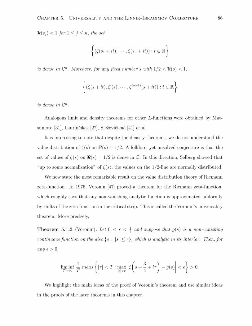
Chapter 5. Universality and the Linnik-Ibragimov Conjecture 86
<(sj) < 1 for 1 ≤ j ≤ n, the set
(ζ(s1 + it), · · · , ζ(sn + it)) : t ∈ R
is dense in Cn. Moreover, for any fixed number s with 1/2 < <(s) < 1,
(ζ(s+ it), ζ ′(s), · · · , ζ(n−1)(s+ it)) : t ∈ R
is dense in Cn.
Analogous limit and density theorems for other L-functions were obtained by Mat-
sumoto [31], Laurincikas [27], Slezeviciene [41] et al.
It is interesting to note that despite the density theorems, we do not understand the
value distribution of ζ(s) on <(s) = 1/2. A folklore, yet unsolved conjecture is that the
set of values of ζ(s) on <(s) = 1/2 is dense in C. In this direction, Selberg showed that
“up to some normalization” of ζ(s), the values on the 1/2-line are normally distributed.
We now state the most remarkable result on the value distribution theory of Riemann
zeta-function. In 1975, Voronin [47] proved a theorem for the Riemann zeta-function,
which roughly says that any non-vanishing analytic function is approximated uniformly
by shifts of the zeta-function in the critical strip. This is called the Voronin’s universality
theorem. More precisely,
Theorem 5.1.3 (Voronin). Let 0 < r < 14
and suppose that g(s) is a non-vanishing
continuous function on the disc s : |s| ≤ r, which is analytic in its interior. Then, for
any ε > 0,
lim infT→∞
1
Tmeas
|τ | < T : max
|s|<r
∣∣∣∣ζ(s+3
4+ iτ
)− g(s)
∣∣∣∣ < ε
> 0.
We highlight the main ideas of the proof of Voronin’s theorem and use similar ideas
in the proofs of the later theorems in this chapter.

Chapter 5. Universality and the Linnik-Ibragimov Conjecture 87
Proof. Let K = s : |s| ≤ r. Since g(s) is non-vanishing on K, we have f(s) = log g(s).
When taking log, we will always assume the principal branch of logarithm. Let Ω be the
set of sequences of real numbers indexed by primes, i.e. ω = (ω2, ω3, · · · ) ∈ Ω. Then, for
any finite subset of primes M , we define the truncated Euler product given by
ζM(s, ω) :=∏p∈M
(1− exp(−2πiωp)
ps
)−1
.
Here, ζM(s, ω) is non-vanishing and analytic on <(s) > 0. So, we can take log and have
log ζM(s, ω) := −∑p∈M
log
(1− exp(−2πiωp)
ps
).
The idea is to approximate f(s) using rearrangements of the summation given above.
Since f is uniformly continuous in the interior of K, there exists κ > 1 such that κ r < 1/4
and
max|s|≤r
∣∣∣∣f( s
κ2
)− f(s)
∣∣∣∣ < ε
2.
Now, f(s/κ2) is analytic and bounded in the region D := s : |s| ≤ R with R = κ r
and thus is an element in the Hardy space, H2(D), which is defined by all functions F (s),
which are analytic on s : |s| < R having finite norm
‖F‖ := limr→R−
∫ ∫|s|≤r|F (s)| dσ dt.
We introduce the inner product on this space, which is defined as
〈F,G〉 = <(∫ ∫
|s|≤RF (s)G(s) dσ dt
).
With the above defined inner product, H2(D) becomes a real Hilbert space. Now,
the key idea is to use Pechersky’s generalization of Riemann’s rearrangement theorem to
Hilbert spaces.

Chapter 5. Universality and the Linnik-Ibragimov Conjecture 88
Theorem 5.1.4 (Pechersky’s rearrangement theorem). Let xn be a sequence in a
complex Hilbert space H satisfying
1.∑∞
n=1 ‖xn‖2 <∞.
2. For 0 6= x ∈ H, the series∑∞
n=1 |〈xn, x〉| diverges to infinity.
Then, the set of all convergent series
∞∑n=1
anxn,
with |an| = 1 is dense in H.
For ω ∈ Ω, let
uk(s, ω) := log
(1− exp(−2πiωpk)
ps+3/4k
).
Consider the series∞∑k=1
uk(s, ω).
Our goal is to apply Pechersky’s theorem 5.1.4 to the above series. From the series
expansion of − log(1− z) = z + z2/2 + z3/3 + · · · , we have that∑∞
k=1 uk(s, ω) differs by
an absolutely convergent series from the series
∞∑k=1
p−(s+3/4)k exp(−2πiωpk)
on |s| < 1/4. Thus, we get the condition 1 for the Pechersky’s theorem from the fact
that∞∑k=1
∣∣∣∣p−3/4+σk
∣∣∣∣2 <∞,for σ < 1/4.
The verification of the condition 2 in Pechersky’s theorem for this application is rather
difficult and involves classical results of Paley and Wiener and Plancherel from Fourier

Chapter 5. Universality and the Linnik-Ibragimov Conjecture 89
analysis, and an application of prime number theorem (see [43, p. 14]).
For the choice of ω = (1/4, 2/4, 3/4, · · · ), using Pechersky’s theorem 5.1.4 there exists
a rearrangement of∑∞
k=1 uk(s, ω) such that
∣∣∣∣∑j
ukj(s, ω)− f(s/κ2)
∣∣∣∣ < ε/4.
The tail of the above series∑
j ukj(s, ω) can be made as small as possible. Say for j > y,
the sum |∑
j>y ukj(s, ω)| < ε/4. Take M a finite set of first n primes such that it contains
all primes appearing in the set pkj for j ≤ y. Thus, we get
max|s|<r
∣∣∣∣ log ζM(s+ 3/4, ω)− f(s)
∣∣∣∣ < ε/4.
The next key idea is to approximate log ζ(s) using log ζM(s).
For E := s = σ + it+ 3/4 : −κr < σ ≤ 2, |t| ≤ 1 and any δ > 0, define
AT :=
τ ∈ [T, 2T ] :
∫E
|ζ−1M (s+ iτ,0)ζ(s+ iτ)− 1|2 dσ dt < δ2
.
Using the approximate functional equation, one can get that for sufficiently large T and
M ,
meas AT > (1− δ)T.
Moreover, by continuity of log ζM(s+ 3/4, ω), for any ε1 > 0, there exists a δ1 such that
if for some ω′ ∈ Ω,
‖ωp − ω′p‖ < δ1
for p ∈M , then
max|s|≤κr
∣∣∣∣ log ζM(s+ 3/4, ω)− log ζM(s+ 3/4, ω′)
∣∣∣∣ < ε1.

Chapter 5. Universality and the Linnik-Ibragimov Conjecture 90
Let
BT :=
τ ∈ [T, 2T ] :
∥∥∥∥τ log p
2π− ωp
∥∥∥∥ < δ1
.
Now using Weyl’s refinement of Kronecker’s approximation theorem on uniformly dis-
tributed curves mod1, it is possible to show that for T sufficiently large
meas BT > cT,
for some positive constant c. Hence, we conclude that
1
Tmeas (AT ∩BT ) > 0,
and the theorem follows.
5.2 Linnik-Ibragimov conjecture
After the result of Voronin, Bagchi [1] gave a proof of universality for the Riemann zeta-
function ζ(s) and some other L-functions using probabilistic methods. Using Bagchi’s
technique, the universality property for many L-functions has been established, mainly
due to the work of Laurancikas, Matsumoto, Steuding et al. In particular, we know that
the universality property holds for elements in the Selberg class S.
Theorem 5.2.1. Let L(s) ∈ S with degree dL. Let K be a compact subset of the strip
1− 1
2dL< <(s) < 1,
with connected complement. Suppose g(s) is any non-vanishing continuous function on
K, which is analytic in the interior of K. Then, for any ε > 0,
lim infT→∞
1
Tmeas
|τ | < T : max
s∈K|L(s+ iτ)− g(s)| < ε
> 0

Chapter 5. Universality and the Linnik-Ibragimov Conjecture 91
It is important to note that the L-functions for which the universality property has
been established is much larger than the Selberg class. In fact, L-functions such as the
Hurwitz zeta-function, Lerch zeta-function or Matsumoto zeta-functions are all known
to be universal in a certain strip. In view of this, Linnik and Ibragimov conjectured the
following.
Conjecture 13. Let F (s) have a Dirichlet series representation, absolutely convergent
on <(s) > 1 and suppose F (s) can be analytically continued to C except for a possible
pole at s = 1 satisfying some “growth conditions”, then F (s) is universal in a certain
strip.
In the next section, we study the universality property for elements in M.
5.3 Main results
Let F ∈ M. Let σc be the abscissa of convergence and σ0 be the abscissa of absolute
convergence of F respectively. Define
σm := inf
σ > σc :
1
T
∫ T
−T|F (σ + it)|2dt T
.
We formulate the Linnik-Ibragimov conjecture more precisely as follows.
Conjecture 14. Let F ∈ M with c∗F > 0. Then, F (s) satisfies the universality property
in the region s ∈ C : σm(F ) < <(s) < σ0(F )
.
Remark 2. The growth condition in Conjecture 13 is captured by c∗F > 0. From Theorem
2.4 of [43], it follows that for F ∈M,
σm(F ) > max
σ0(F )− 1
2, σ0(F )− 1
2c∗F
.

Chapter 5. Universality and the Linnik-Ibragimov Conjecture 92
This gives a non-trivial region for the strip of universality of F .
We state the main results of this chapter below which give some indicative evidence
towards Conjecture 14 for elements in M. Henceforth, for an open set D ⊆ C, H(D)
denotes the space of holomorphic functions on D with L2-topology.
Theorem 5.3.1. For F ∈M with c∗F > 0, let D denote the vertical strip
s ∈ C : σm < <(s) < σ0
.
There exists a sequence of functions Fn converging to F in H(D), such that each of the
Fn is universal in the vertical strip s ∈ C : σm(Fn) < <(s) < σ0(Fn).
Let K be a compact set in the strip s ∈ C : σm < <(s) < σ0 with connected
complement. We say that a function g(s) defined on K is ε-approximable by F (s) ∈M if
for a given ε > 0, we can find a δ > 0 and a sequence Fn of universal functions converging
to F in the strip as in Theorem 5.3.1, such that
lim infT→∞
1
Tmeas
τ | < T : max
s∈K|Fn(s+ iτ)− g(s)| < ε/2
> δ,
for all T > Tε, for some large Tε depending on ε.
Theorem 5.3.2. Suppose F ∈ M with c∗F > 0 and D be as in Theorem 5.3.1. Let K be
a compact set in D with connected complement. Let g(s) be a continuous function on K,
holomorphic in the interior of K, and ε-approximable by F (s). Then,
lim infT→∞
1
Tmeas
|τ | < T : max
s∈K|F (s+ iτ)− g(s)| < ε
> 0.

Chapter 5. Universality and the Linnik-Ibragimov Conjecture 93
5.4 Limit and Density Theorems
In this section, we introduce some tools and results to be used in the proof of Theoerm
5.3.1 and 5.3.2.
For any topological space S, denote by B(S) the class of Borel sets of S. Let γm :=
s ∈ C : |s| = 1. Define the infinite dimensional torus
Ω :=∞∏m=1
γm.
By inducing the product topology and pointwise multiplication, Ω forms a compact
abelian group. Thus, we have the normalized Haar measure mH on Ω, which generates a
probability space (Ω, B(Ω),mH). Denote by ω(m) the projection of ω ∈ Ω onto γm. Then,
ω(m) : m ∈ N is a sequence of independent random variables defined on (Ω, B(Ω),mH).
We state the limit theorem due to Laurancikas, Steuding and Schwarz [25].
Theorem 5.4.1. Let f(s) =∑∞
m=1 amω(m)e−λms with ω ∈ Ω and λm, a Q-linearly
independent set. Let D := s ∈ C : <(s) > σm and DM := s = σ + it ∈ C : σm < σ <
σ0, |t| < M satisfy the following properties.
1. |F (s)| |t|α for some α > 0, where σm < σ < σ0.
2. For σm < σ < σ0, ∫ T
−T|F (σ + it)|2dt T.
3. λm ≥ c(logm)δ for some c, δ > 0.
Then, the probability measure
ν(F (s+ iτ) ∈ A), for A ∈ B(H(DM))

Chapter 5. Universality and the Linnik-Ibragimov Conjecture 94
converges weakly to PF as T →∞, where
PF (A) := mH(ω ∈ Ω : F (s, ω) ∈ A) for A ∈ B(H(DM)).
If F ∈ M, then∑
n an/ns =
∑n ane
−s logn. Unfortunately, log n is not Q-linearly
independent. Thus, we do not have the limit theorem as above.
Consider a sequence E = en with 0 < en < 1. Define
FE(s) :=∞∑n=1
ane−s log (n+en).
Lemma 5.4.2. If F ∈M, then σc(F ) = σc(FE) and σ0(F ) = σ0(FE).
Proof. Suppose the Dirichlet series of F given by F (s) =∑
n an/ns is convergent in the
region <(s) > σc. Note that
(anns− an
(n+ en)s
)=anns
(1− ns
(n+ en)s
).
For σ ∈ R, note that
1−(
n
n+ en
)σ en|σ|
n.
Thus, we get that the series
∞∑n=1
annσ
(1− nσ
(n+ en)σ
)
is absolutely convergent for σ > σc. Hence, the general Dirichlet series given by
G(s) :=∞∑n=1
[anns− an
(n+ en)s
]
is convergent for real σ > σc. By Theorem 1 of [20, p.3] we have the abscissa of conver-
gence for the general Dirichlet series G(s) is ≤ σc. Using FE(s) = F (s) − G(s), we get

Chapter 5. Universality and the Linnik-Ibragimov Conjecture 95
the abscissa of convergence for FE as ≤ σc. Since the abscissa of convergence for F (s) is
σc, we get the abscissa of convergence for FE(s) is also σc.
By a similar argument, we also get σ0(FE) = σ0(F ).
For every n ∈ N and given 0 < δn < e−n, there exists E = εn such that εn < δn
and log(n + εn)∞n=1 is a Q-linearly independent set. We see this by induction. For
n = 1, choose any ε1 < δ1 such that log(1 + ε1) 6= 0. Suppose log(1 + ε1), · · · , log(n +
εn) is a Q-linearly independent set. Consider the Q-vector space Wn generated by
log(1 + ε1), · · · , log(n + εn). Since Wn is a finite dimensional vector space over Q, it
is countable. So, we can find εn+1 ∈ (0, δn+1) such that log(n + 1 + εn+1) /∈ Wn. Thus,
log(1+ ε1) · · · log(n+1+ εn+1) is a Q-linearly independent set. We proceed inductively
to construct log(n+ εn)∞n=1, which is a Q-linearly independent set. Define
FE(s) :=∞∑n=1
ane−s log(n+εn).
By our choice of E, we have σ0 and σc of FE is same as that of F . Moreover, FE(s)
satisfies the Limit Theorem 5.4.1. We first show the universality property for FE in the
strip s ∈ C : σm(FE) < <(s) < σ0(FE). We proceed as in [28].
Denote
DW := s ∈ C : σm(FE) < <(s) < σ0(FE), |=(s)| < W
The next goal is to show that the support of PFE is H(DW ).
Let S be a separable topological space and P be a probability measure on (S,B(S)).
Recall that the support of P in S is defined as
SP :=⋂
P (C)=1,C closed
C.

Chapter 5. Universality and the Linnik-Ibragimov Conjecture 96
In other words,
SP = x ∈ S : P (U) > 0, for any neighbourhood U of x.
Let X be an S-valued random element on a probability space (Ω,F, P ), then the
support of the random variable X, denoted by SX , is the support of the distribution
P (X ∈ A), where A ∈ B(S).
We are now ready to prove the main lemma of this section. Let ω(m) : m ∈ N be a
sequence of independent random variables defined on (Ω, B(Ω),mH) as described above.
For any such ω(m), define
gm(s) = amω(m)e−s log(n+εn)
Then we have the following proposition.
Proposition 5.4.3. Let gm(s) be as above. The set of all convergent series∑
m gm(s) is
dense in H(DW ).
Proof. We use the following theorem (see [26], Theorem 6.3.10).
Theorem 5.4.4. Let D be a simply connected domain in C. Let fm be a sequence in
the space H(D) satisfying the following properties.
1. Let µ be a complex measure on (C, B(C)) with compact support contained in D such
that∞∑m=1
∫Cfmdµ <∞.
Then,∫C s
rdµ(s) = 0 for all r ∈ N ∪ 0.
2. The series∑∞
m=1 fm converges in H(D).

Chapter 5. Universality and the Linnik-Ibragimov Conjecture 97
3. For any compact K ∈ D,∞∑m=1
sups∈K|fm(s)|2 <∞.
Then, the set of all convergent series
∞∑m=1
bmfm,
with |bm| = 1 for all m is dense in H(D).
To prove the proposition, consider any complex measure µ on (C, B(C)) with compact
support contained in DW , such that
∞∑m=1
sups∈K|gm(s)|2 <∞.
In order to conclude that∫C s
rdµ(s) = 0 for r = 0, 1, 2, · · · , we first set some notations.
Let FE(s) =∑
n an/(n + εn)s be as above with abscissa of absolute convergence σ0
and let
cn :=an
(n+ εn)σ0.
For any complex measure µ on (C, B(C)) with compact support on DW , denote
ρ(s) :=
∫Ce−szdµ(z).
We use the following Lemma (see Lemma 5 of [28])
Lemma 5.4.5. For any complex measure µ on (C, B(C)) with compact support on DW ,
if∞∑n=1
|cn||ρ(λn)| <∞,
then ∫Csrdµ(s) = 0,

Chapter 5. Universality and the Linnik-Ibragimov Conjecture 98
for r = 0, 1, 2, · · ·
Using Lemma 5.4.5, we see that gm(s) satisfies all the conditions in the Theorem
5.4.4. Moreover, from [25], we also know that for almost all ω ∈ Ω,
∞∑m=1
am ω(m)
(m+ εm)s
converges uniformly on compact sets on the right half plane s : <(s) > σc. Hence,
applying the Theorem 5.4.4, we have the proposition.
5.5 Proof of the main theorems
In this section, we use the tools introduced earlier to prove Theorem 5.3.1 and 5.3.2. We
first show that FE(s) is universal, where
FE(s) :=∞∑n=1
an(n+ εn)s
and log(n + εn) is a Q-linearly independent set. To prove this, we use the following
theorem (see Theorem 1.7.10 of [26]).
Theorem 5.5.1. Let Xn be a sequence of independent H(DW )-valued elements such
that∑∞
m=1 Xm converges almost surely. Then, the support of the sum∑∞
m=1Xm is the
closure of all g ∈ H(DW ), which may be written as the convergent series
g =∞∑m=1
gm,
for gm ∈ SXm.
Using Theorem 5.5.1 and Proposition 5.4.3, we show that PFE is supported on the
whole of H(DW ).

Chapter 5. Universality and the Linnik-Ibragimov Conjecture 99
Proposition 5.5.2. The support of the measure PFE is H(DW ).
Proof. The sequence ω(m) defined above is a sequence of independent random variables
on the probability space (Ω, B(Ω),mH), where the support of every ω(m) is the unit circle.
Therefore amω(m)e−s log(m+εm) is a sequence of H(DW )-valued random elements and
the support of each element is given by
g ∈ H(DW ) : g(s) = amb e
−s log(m+εm), with |b| = 1
.
Therefore, by Theorem 5.5.1, the support of H(DW )-valued random element
F (s, w) :=∞∑m=1
amω(m)e−s log(m+εm)
is the closure of the set of all convergent series∑
m ambme−s log(m+εm), with |bm| = 1. By
Proposition 5.4.3, we are done.
We now show that FE(s) is universal.
Proposition 5.5.3. Suppose FE is defined as above. Let K be a compact subset of
D = s ∈ C : σm < <(s) < σ0 with connected complement. Let g(s) be a continuous
function on K, holomorphic in the interior of K. Then, for any ε > 0,
lim infT→∞
1
Tmeas
|τ | < T : max
s∈K|FE(s+ iτ)− g(s)| < ε
> 0.
Proof. Let K be a compact set in D with connected complement. Then, there exists a
DW such that K ⊆ DW . We first show that vertical shifts of FE(s) approximate any
polynomial p(s) over DW up to ε. Consider the following open set in H(DW ).
G :=
f ∈ H(DW ) : |f(s)− p(s)| < ε, for s ∈ DW
.

Chapter 5. Universality and the Linnik-Ibragimov Conjecture 100
Since G is open, by Proposition 5.5.2 and Theorem 5.4.1, we get
lim infT→∞
1
Tmeas
|τ | < T : sup
s∈K|FE(s+ iτ)− p(s)| < ε
≥ PFE(G) > 0.
We prove the assertion for any function g(s) continuous on K and holomorphic in its
interior by finding a polynomial approximation to g(s) on K.
Next, we prove the Theorem 5.3.1. In other words, we show that any F ∈ M is a
limit point of functions FEm , which are universal in the vertical strip Dm = s ∈ C :
σm(FEm) < <(s) < σ0(FEm). It suffices to show the following lemma.
Lemma 5.5.4. For any given ε, T > 0, there exists an E = εn such that
|F (s)− FE(s)| < ε,
for s ∈ DT := s = σ + it ∈ C : σm(F ) < <(s) < σ0(F ), |t| < T.
Proof. For any fixed n, small δn > 0, and a fixed T > 0, we can find εn > 0, such that
∣∣∣∣1− ns
(n+ εn)s
∣∣∣∣ ≤ δn (5.1)
for s ∈ DT . This is because
n
n+ εn= 1− εn
n+ εn.
Therefore for s = σ + it,
(n
n+ εn
)s=
(1− εn
n+ εn
)σexp
(it log
(1− εn
n+ εn
)).

Chapter 5. Universality and the Linnik-Ibragimov Conjecture 101
Since |t| < T , using
(1− εn
(n+ εn)
)σ 1− |σ|εn
(n+ εn)and
log
(1− εn
(n+ εn)
) εn
(n+ εn),
we can choose a sufficiently small εn such that (5.1) holds.
For an 6= 0, choose δn as
δn =ε
2n
∣∣∣∣nσm(F )
an
∣∣∣∣.Thus, we have ∣∣∣∣anns
(1− ns
(n+ εn)s
)∣∣∣∣ ≤ ε
2n.
for all s ∈ DT . By summing over all n, we conclude that
∣∣∣∣ ∞∑n=1
anns−∞∑n=1
an(n+ εn)s
∣∣∣∣ < ε,
for s ∈ DT . Hence, we have the lemma.
From Lemma 5.5.4, it is clear that for any F ∈M, we can find a sequence En, such
that FEn converges to F and each FEn(s) is universal in the strip σm(FEn) < <(s) <
σ0(FEn). Hence, we have Theorem 5.3.1.
For Theorem 5.3.2, we suppose that for an ε > 0, g(s) is continuous on K ⊆ D and
analytic in the interior of K and ε-approximable by F (s).
We can find a sequence FEn of functions universal in D such that |FEn(s+it0)−g(s)| <
ε/2 for infinitely many t0 and further there exists a δ > 0 and Tε > 0 such that
meas
|τ | < T : max
s∈K|FEn(s+ iτ)− g(s)| < ε/2
≥ δT,
with δ > 0 fixed, for all T > Tε.
By Theorem 5.3.1, for any given T > Tε we can find a subsequence FEn of functions

Chapter 5. Universality and the Linnik-Ibragimov Conjecture 102
universal in D such that
|F (s)− FEn(s)| < ε/2
for s ∈ DT .
By triangle inequality, we have
|F (s+ iτ)− g(s)| ≤ |F (s+ iτ)− FEn(s+ iτ)|+ |FEn(s+ iτ)− g(s)|.
Hence, we conclude for T Tε as chosen above,
meas
|τ | < T : max
s∈K|F (s+ iτ)− g(s)| < ε
T.
This proves Theorem 5.3.2.
5.6 The Generalized Strong Recurrence
Bohr studied the notion of almost periodicity for Dirichlet series. Any analytic function
f(s) is said to be almost periodic in a vertical strip σ1 < <(s) < σ2, if for any ε > 0, we
can find a length l > 0, such that for any interval of length l, there exists a τ ∈ (θ, θ+ l)
satisfying
|f(s+ iτ)− f(s)| < ε,
for a fixed s in the vertical strip σ1 < <(s) < σ2.
Bohr showed that any Dirichlet series is almost periodic in its half plane of absolute
convergence. Moreover, he also discovered interesting connections between the Riemann
hypothesis and the almost periodicity of L-functions. In fact, he showed that Riemann
hypothesis for any Dirichlet L-function L(s, χ), where χ is a non-principal primitive
character, is equivalent to almost periodicity of L(s, χ) in the right half plane <(s) > 1/2.
In 1981, Bagchi [1] observed that a similar notion of almost periodicity in the sense

Chapter 5. Universality and the Linnik-Ibragimov Conjecture 103
of universality is equivalent to the Riemann hypothesis. A refined version of Bagchi’s
theorem can be stated as follows.
Theorem 5.6.1 (Bagchi). Let θ ≥ 1/2. Then ζ(s) is non-vanishing in the half plane
<(s) > θ if and only if, for ε > 0, any z with θ < <(z) < 1, and for any 0 < r <
min<(z)− θ, 1−<(z),
lim infT→∞
1
Tmeas
τ ∈ [0, T ] : max
|s−z|≤r|ζ(s+ iτ)− ζ(s)| < ε
> 0.
The above equivalent formulation of Riemann hypothesis is called the property of
strong recurrence. We sketch a proof of the above theorem.
Proof. If the Riemann hypothesis is true, then we clearly have the strong recurrence as
a consequence of Voronin’s universality theorem.
On the other hand, if the strong recurrence is true and there is a zero of ζ(s) with
s = σ + it satisfying 1/2 < σ < 1, then we will produce a large number of zeroes of ζ(s)
in the vertical strip σ < <(s) < 1, which would violate the zero-density theorem.
Suppose ρ is a zero of ζ(s) with <(ρ) > θ. Consider a neighbourhood around ρ, given
by
Hδ := s : |s− ρ| < δ.
Assuming the strong recurrence, we can find τ > 0 such that
|ζ(s+ iτ)− ζ(s)| < ε,
for s ∈ Hδ. Taking ε sufficiently small, Rouche’s theorem ensures a zero of ζ(s) in
the region Hδ + iτ . Moreover, the strong recurrence also ensures that the number of
occurrences of τ is proportional to the vertical height T . Hence, we get the number of
zeroes of ζ(s) in the region <(s) > θ and |=(s)| < T is Ω(T ), which violates the density

Chapter 5. Universality and the Linnik-Ibragimov Conjecture 104
theorem 2.9,
N(θ, T ) T 4θ(1−θ)+ε1 .
In class M, although we do not have the Riemann hypothesis, we might expect to
have a strong recurrence property.
We end by stating the analogue of Riemann hypothesis for the class M in terms of
the strong recurrence property.
Conjecture 15 (Generalized Strong Recurrence). Let F ∈M. For any ε > 0 and any z
with σm(F ) < <(z) < σ0(F ), and for any 0 < r < min<(z)− σm(F ), σ0(F )−<(z),
lim infT→∞
1
Tmeas
τ ∈ [0, T ] : max
|s−z|≤r|F (s+ iτ)− F (s)| < ε
> 0.

Bibliography
[1] B. Bagchi, The statistical behaviour and universality properties of the Riemann zeta-
function and other allied Dirichlet series, PhD Thesis , Indian Statistical Institute,
Calcutta, (1981).
[2] H. Bohr, Uber das Verhalten von ζ(s) in der Halbebene σ > 1, Nachr. Akad. Wiss.
Gottingen II Math. Phys. Kl., pp. 409-428, (1911).
[3] H. Bohr, Uber eine quasi-periodische Eigenschaft Dirichletscher Reihen mit Anwen-
dung auf die Dirichletschen L-Funktionen, Math. Annalen., 85, pp. 115-122, (1922).
[4] H. Bohr, B. Jessen, Uber die Werteverteilung der Riemannschen Zetafunktion, erste
Mitteilung, Acta Mathematica, 54, pp. 1-35, (1930).
[5] H. Bohr, B. Jessen, Uber die Werteverteilung der Riemannschen Zetafunktion, erste
Mitteilung, Acta Mathematica, 58, pp. 1-55, (1932).
[6] H. Bohr, E. Landau, Sur Les zeros de la fonction ζ(s) de Riemann, Comptes Rendus
Acad. Sci. Paris, 158, pp. 106-110, (1914).
[7] E. Bombieri and H. Iwaniec, On the order of ζ(1/2 + it), Ann. Scuola Norm. Sup.
Pisa Cl. Sci.(4), 13, pp. 449-472, (1986).
[8] E.Bombieri and D.A.Hejhal, On the distribution of zeros of linear combinations of
Euler products, Duke Math. J., 80, pp. 821–862, (1995).
105

Bibliography 106
[9] E. Bombieri and A. Perelli, Zeros and poles of Dirichlet series, Rend. Mat. Acc. Lincei
12, pp. 69-73, (2001).
[10] F. Carlson, Contributions a la theorie des series de Dirichlet. I, Arkiv for Mat. Astr.
och Fysik, 16, (1922).
[11] F. Carlson, Contributions a la theorie des series de Dirichlet. II, Arkiv for Mat. Astr.
och Fysik, 19, (1926).
[12] B. Conrey and A. Ghosh, On the Selberg class of Dirichlet series: small degrees,
Duke Math. J., 72, pp. 673-693, (1993).
[13] B. Conrey and A. Ghosh, Remarks on the generalized Lindelof hypothesis, Func-
tiones et Approximatio, 36, pp. 71–78, (2006).
[14] Anup B. Dixit, Value distribution of L-functions, submitted. ( arXiv:1711.06671 )
[15] Anup B. Dixit, On the Linnik-Ibragimov conjecture, in preparation.
[16] A.B. Dixit and V.K. Murty, The Lindelof Class of L-functions (II), pre-print.
[17] P. Epstein, Zur Theorie allgemeiner Zetafunktionen I, Math. Annalen, 56, pp.
615–644, (1903).
[18] P. Epstein, Zur Theorie allgemeiner Zetafunktionen II, Math. Annalen, 63, pp.
205–216, (1907).
[19] A.A. Goldberg and I.V. Ostrovskii, Value Distribution of Meromorphic Functions,
American Mathematical Society, Provindence, (2008).
[20] G.H.Hardy, Marcel Riesz, The General Theory of Dirichlet Series, Cambridge
University Press, 1915.
[21] T. Hattori, K. Matsumoto, A limit theorem for Bohr-Jessen’s probability measures
for the Riemann zeta-function, J. Reine Angew. Math., 507, pp. 219-232, (1999).

Bibliography 107
[22] W.H. Hayman, Meromorphic Functions, Oxford University Press, (1964).
[23] J. Kaczorowski, A. Perelli, On the structure of the Selberg class, I: 0 ≤ d ≤ 1, Acta
Math.182, pp. 207-241, (1999).
[24] J. Kaczorowski, A. Perelli, On the prime number theorem in the Selberg class Arch.
Math, 80, pp. 255-263, (2003).
[25] A. Laurincikas W. Schwarz, J. Steuding. Value distribution of general Dirichlet se-
ries III, Proceedings of the Third International Conference in honour of J. Kubilius,
Palanga, 2001.
[26] A. Laurincikas, Limit theorems for Riemann zeta-function, Kluwer Academic Pub-
lishers, Dordrecht, 1996.
[27] A. Laurincikas, A limit theorem for Dirichlet L-functions, Mat. Zametki, 25, pp.
481-485, (1979).
[28] A. Laurincikas W. Schwarz, J. Steuding., The universality of general Dirichlet series,
Analysis, 23, pp. 13-26, (2003).
[29] Bao Qin Li, A result on value distribution of L-functions, Proceedings of the Amer-
ican Mathematical Society, 138, pp. 2071-2077, (2010).
[30] Bao Qin Li, A uniqueness theorem for Dirichlet series satisfying Riemann type func-
tional equation, Advances in Mathematics, 226, pp. 4198-4211, (2011).
[31] K. Matsumoto, Value-Distribution of Zeta-Functions, in Analytic Number Theory,
Proceedings of the Japanese-French Symposium, Tokyo, (1988), eds. K. Nagasaka and
E. Fouvry, Lecture Notes in Maths 1434, Springer, Berlin Heidelberg New York, pp.
178-187, (1990).
[32] Giuseppe Molteni, On the algebraic independence in the Selberg class, Archiv der
Mathematik79, pp. 432-438, (2002).

Bibliography 108
[33] Giuseppe Molteni, General linear independence of a class of multiplicative functions,
Arch. Math., 83, pp. 27-40 (2004).
[34] V. K. Murty, The Lindelof Class of L-functions, pp. 165-174, eds. L. Weng and M.
Kaneko, World Scientific, (2007).
[35] M. R. Murty, Selberg’s conjectures and Artin L-functions, Bull. Amer. Math. Soc.,
31, pp. 1-15, (1994).
[36] M. R. Murty, Selberg’s conjectures and Artin L-functions, II, Current Trends in
Mathematics and Physics, S.D. Adhikari, (Ed.), Narosa, New Delhi, pp.154-168,
(1995).
[37] M.R. Murty, Selberg’s conjectures and Artin L-functions, Bulletin of American
Mathematical Society, 31, pp. 1-14, (1994).
[38] M.R. Murty and V.K. Murty, Strong multiplicity one for Serlberg’s class, C.R. Acad.
Sci. Paris Ser, I Math. 319 (1994), pp 315-320.
[39] R. Nevanlinna, Einige Eindeutigkeitssatze in der Theorie der Meromorphen Funk-
tionen, no. 3-4, Acta Math.,48, pp. 367-391, (1926).
[40] A. Selberg, Old and new conjectures and results about a class of Dirichlet series,
Collected Papers, 2, pp. 47-63, Springer-Verlag, Berlin Heidelberg New York, (1991).
[41] , R. Slezeviciene, Joint limit theorems and universality for the Riemann and allied
zeta-functions, PhD thesis, Vilnius University, (2002).
[42] J.Steuding, On the value-distribution of L-functions, Fiz. Mat. Fak. Moksl. Semin,
Darb, 6, pp 87-119, (2003).
[43] J. Steuding, Value-Distribution of L-functions, Lecture notes in mathematics,
Springer, (2007).

Bibliography 109
[44] J. Steuding, How many values can L-functions share?, Fizikos ir mathematikos fakul-
teto, 7, pp. 70-81, (2004).
[45] E.C. Titchmarsh, The theory of Riemann-Zeta function, Second edition, revised by
D.R. Heath-Brown, Clarendon Press-Oxford, (1986).
[46] S.M. Voronin, The distribution of non-zero values of Riemann zeta-function, Izv.
Akad. Nauk Inst. Steklov, 128, pp. 131-150, (1972).
[47] S.M. Voronin, Theorem on ’universality’ of the Riemann zeta function, Izv. Akad.
Nauk SSSR, Ser. Matem., 39, pp. 475-486, (1975).
[48] Z. Ye, The Nevanlinna functions of the Riemann zeta-function, Journal of Mathe-
matical Analysis and Applications, 233, pp 425-435, (1999)