the limited rademacher functions and bernoulli ... · •the hausdorff dimension of the graph of...
TRANSCRIPT

Advances in Mathematics 195 (2005) 24–101
www.elsevier.com/locate/aim
The limited Rademacher functions and Bernoulliconvolutions associated with Pisot numbers
De-Jun Feng1
Department of Mathematical Sciences, Tsinghua University, Beijing 100084, PR China
Received 21 January 2004; accepted 28 June 2004
Communicated by R.D. MauldinAvailable online 11 September 2004
Abstract
In this paper, we give a systematical study of the local structures and fractal indices of thelimited Rademacher functions and Bernoulli convolutions associated with Pisot numbers. For agiven Pisot number in the interval(1,2), we construct a finite family of non-negative matrices(maybe non-square), such that the corresponding fractal indices can be re-expressed as somelimits in terms of products of these non-negative matrices. We are especially interested in thecase that the associated Pisot number is a simple Pisot number, i.e., the unique positive root ofthe polynomialxk−xk−1− . . .−x−1 (k=2,3, . . .). In this case, the corresponding products ofmatrices can be decomposed into the products of scalars, based on which the precise formulasof fractal indices, as well as the multifractal formalism, are obtained.© 2004 Elsevier Inc. All rights reserved.
MSC: primary 28A78; secondary 28D20; 58F11; 54C30; 11R06
Keywords:Limited Rademacher functions; Bernoulli convolutions; Pisot numbers; Hausdorff dimension;Information dimension;Lq -spectrum; Multifractals; Product of matrices
1. Introduction
In this paper, we provide a systematical study of the local structures and differentfractal indices of the limited Rademacher functions and Bernoulli convolutions associ-ated with Pisot numbers. We also verify the validity of the multifractal formalism for
E-mail address:[email protected] supported by the Special Funds for Major State Basic Research Projects in China.
0001-8708/$ - see front matter © 2004 Elsevier Inc. All rights reserved.doi:10.1016/j.aim.2004.06.011

D.-J. Feng /Advances in Mathematics 195 (2005) 24–101 25
the corresponding Bernoulli convolutions associated with a special class of Pisot num-bers. Recall that a real algebraic integer is called aPisot numberif all its conjugatesare less than 1 in modulus. There are infinitely many Pisot numbers in the interval(1,2): for example, for eachk = 2,3, . . ., the unique positive root of the polynomial
pk(x) = xk − xk−1− xk−2− · · · − x − 1
is a Pisot number. We shall call these thesimplePisot numbers. The readers may seethe books[3,55] for the detailed properties of Pisot numbers.Recall that for 12 < � < 1, the limited Rademacher function fwith parameter� is
defined by
f (x) = (1− �)∞∑n=0
�nR(2nx), x ∈ [0,1], (1.1)
whereR denotes the classic Rademacher function:R(x) is defined on the lineR withperiod 1, taking values 0 and 1 on the intervals[0, 12) and [12,1), respectively. Thedistribution of f induces a probability measure� on [0,1]. That is,
�(E) = L{x ∈ [0,1] : f (x) ∈ E}, ∀ Borel setE ⊂ [0,1],
where L denotes the one-dimensional Lebesgue measure. The measure� is calledthe Bernoulli convolutionwith parameter�, since it is the infinite convolution of12(�0+�(1−�)�n). An important property of� is its self-similarity (see, e.g.,[31, Theorem4.3]):
� = 12 � ◦ S−10 + 1
2 � ◦ S−11 , (1.2)
whereS0(x) = �x and S1(x) = �x + 1− �.The limited Rademacher functions and Bernoulli convolutions have been studied for
a long time, revealing many connections with harmonic analysis, number theory, fractalgeometry and dynamical systems, see[1,30,48,53,57]. It is well known [28] that foreach parameter� ∈ (1/2,1), � is either absolutely continuous or totally singular. Erdös[6] proved that� is totally singular if � is the reciprocal of a Pisot number. In theopposite direction, Solomyak [56] proved that� is absolutely continuous withd�
dx∈ L2
for almost all� ∈ (1/2,1), extending an early result of Erdös [7]. Please see [49] fora simpler proof. Mauldin and Simon [39] showed that� is in fact equivalent to theLebesgue measure for almost all� ∈ (1/2,1). Later Peres and Schlag [47] strengthedSolomyak’s result by showing the Hausdorff dimension of the exceptional�’s in [a,1]is strictly smaller than 1 for eacha > 1
2. Recently, Feng and Wang [20] found asequence of�’s such that�−1 is not Pisot number and� lies in the exceptional set(i.e. the corresponding�, if it is absolutely continuous, has noL2 density).In this paper, we always assume that the parameter� ∈ (12,1) is a Pisot reciprocal.
That is, �−1 is a Pisot number. Under this assumption, we would like to analyse

26 D.-J. Feng /Advances in Mathematics 195 (2005) 24–101
the complexity and the degree of singularity of the corresponding limited Rademacherfunction and Bernoulli convolution. More precisely, we study the following fractalindices for a fixed Pisot reciprocal�:
• the Hausdorff dimension of the graph of the limited Rademacher function;• the Hausdorff dimension of the level sets of the limited Rademacher function;• the Lq -spectrum, Hausdorff dimension and the range of local dimensions of theBernoulli convolution.
Furthermore, we will give a complete multifractal analysis of� when � is a simplePisot number.Our basic approach is the following: using an algebraic property of Pisot numbers
found by Garcia[22], for each given Pisot reciprocal� in (1/2,1) we construct afinite family of non-negative matrices (maybe non-square) and re-express a major partof the above fractal indices as limits in terms of products of these matrices. Particularlyinteresting is the case where� is the reciprocal of a simple Pisot number. In this casewe find that the corresponding product of matrices is degenerate and can be decomposedas the product of a sequence of scalars (this fact implies that� is locally a self-similarmeasure with countably many generators which satisfy the separation condition). Usingthis key property, we obtain the precise formulas of all the above fractal indices, andverify the validity of the multifractal formalism of�.At first we give some necessary definitions and notations. We use dimH, dimB to
denote the Hausdorff dimension and the box-counting dimension, respectively (see[8,38] for the definitions). For a real functiong defined on[0,1], the graph of thefunction g, denoted as�(g) or simply �, is defined by
� = {(x, g(x)) ∈ R2 : x ∈ [0,1]}.
For t ∈ R, the t-level setof g, denoted asLt(g) or simply Lt , is defined by
Lt = {x ∈ [0,1] : g(x) = t}.
For a given finite Borel measure� on the line, theupper local dimension of� atx ∈ supp(�) is defined by
d(�, x) = lim supr→0+
log�([x − r, x + r])logr
,
and the lower local dimensiond(�, x) at x is defined similarly by taking the lowerlimit. When d(�, x) = d(�, x), the common value is called thelocal dimensionof � atx and is denoted byd(�, x). The range of local dimensions of�, denoted byR(�), isdefined by
R(�) = {y ∈ R : d(�, x) = y for somex ∈ supp(�)}.

D.-J. Feng /Advances in Mathematics 195 (2005) 24–101 27
Recall theHausdorff dimensionof � is defined by
dimH(�) = inf {dimH(E) : E ⊂ R is a Borel set and�(E) = 1} ,
and theLq -spectrum(q ∈ R) of � is defined by
�(q) = �(�, q) = lim inf�→0+
log(sup
∑i �([xi − �, xi + �])q)
log�,
where the supremum is taken over all the families{[xi−�, xi+�]}i of disjoint intervalswith xi ∈ supp(�). The readers may see the books[8,38,50,60] for more informationabout the above definitions.We will state our matrix product results for general Pisot reciprocals in Section 3.
In the following we only present our results for the cases� = �k (k = 2,3, . . .), where�k is the largest real root ofxk+xk−1+· · ·+x−1. Define two 2×2 matricesM0,M1by
M0 =[1 10 1
], M1 =
[1 01 1
]. (1.3)
For n�1, denote byAn the set of all indicesj1 . . . jn over {0,1}. DenoteMJ = Mj1Mj2 . . .Mjn
for J = j1 . . . jn. For our convenience, we write∅ for the empty word and define
M∅ =[1 00 1
].
Set A0 = {∅}. For any 2× 2 non-negative matrixB, denote its norm by‖B‖ =(1,1)B(1,1)T .Our main results for the cases� = �k (k�2) are the following theorems:
Theorem 1.1. For k = 2,3, . . ., let � be the graph of the limited Rademacher functionf with parameter� = �k. Then
dimH � = logxklog�
,
wherexk is the unique root in(0, �k−1) (defining�1 = 1) of the equation
1− 2xk−1+ xk1− 2x + xk ·
∞∑n=0
∑J∈An
‖MJ ‖�k xkn+k+1 = 1
with �k = − log�log 2.

28 D.-J. Feng /Advances in Mathematics 195 (2005) 24–101
Theorem 1.2. For k = 2,3, . . ., the Hausdorff dimension and box-counting dimen-sion of t-level set of the limit Rademacher function f with parameter� = �k areequal to
dk := �k(1− 2�k
)2(2− (k + 1)�k
)log 2
∞∑n=0
�kn∑J∈An
log‖MJ ‖
for L almost all t ∈ [0,1].
Theorem 1.3. (i) For any q ∈ R, the Lq -spectrum�(q) of the Bernoulli convolutionwith parameter� = �2 is equal to
−q log 2log�
− logx(2, q)
log�,
wherex(2, q) is defined by
x(2, q) = sup
x�0 :∞∑n=0
∑J∈An
‖MJ ‖q x2n+3�1
.There exists a unique real numberq0 < −2 satisfying
∞∑n=0
∑J∈An
‖MJ ‖q0 = 1.
For q > q0, x(2, q) is the unique positive root of
∞∑n=0
∑J∈An
‖MJ ‖q x2n+3 = 1,
and it is an infinitely differentiable function of q on(q0,+∞). For q�q0, x(2, q) = 1.Moreoverx(2, q) is not differentiable atq = q0.(ii) For any integer k�3 and any real number q, the Lq -spectrum�(q) of the
Bernoulli convolution� with parameter� = �k is equal to
−q log 2log�
− logx(k, q)
log�,

D.-J. Feng /Advances in Mathematics 195 (2005) 24–101 29
Table 1Numerical estimations
k dimH �(f�k ) d�k dimH ��k
2 1.304± 0.001 0.302±0.001 0.9957±10−43 1.11875217± 10−8 0.1025001503±10−10 0.98040931953±10−114 1.052565407±10−9 0.041560454940769±10−14 0.9869264743338±10−125 1.024596045±10−9 0.01842625239655±10−14 0.9925853002741±10−126 1.011844824±10−9 0.00859023108854±10−14 0.9960325915849±10−127 1.005796386±10−9 0.00412363866083±10−14 0.9979374455070±10−128 1.002862729±10−9 0.00201383805752±10−14 0.9989449154498±10−129 1.001421378±10−9 0.00099344117302±10−14 0.9994653680555±10−1210 1.000707890±10−9 0.00049294459129±10−14 0.9997306068783±10−12
wherex(k, q) ∈ (0, �k−1) satisfies
1− 2xk−1+ xk1− 2x + xk ·
∞∑n=0
∑J∈An
‖MJ ‖q xkn+k+1 = 1.
Moreoverx(k, q) is an infinitely differentiable function of q on the whole line.
Theorem 1.4. For k = 2,3, . . ., the Hausdorff dimension of the Bernoulli convolution� with parameter� = �k satisfies
dimH � = − log 2
log�+(2k − 3
2k − 1
)2
·
∞∑n=0
2−kn−k−1∑J∈An
‖MJ ‖ log‖MJ ‖
log�.
Theorem 1.5. For k = 2,3, . . ., let R(�) be the range of local dimensions of theBernoulli convolution� with parameter� = �k. Then
R(�) =
[− log 2
log� − 12,− log 2
log�
]if k = 2,
[− k log 2(k+1) log� , − log 2
log�
]if k�3.
In Table 1, we give some numerical estimations of dimH �, dk and dimH � in theabove theorems for 2�k�10.
Theorem 1.6. For k = 2,3, . . ., let � be the Bernoulli convolution� with parameter� = �k. For each��0, define
K(�) ={x ∈ [0,1] : lim
�→0
log�([x − �, x + �])log�
= �}.

30 D.-J. Feng /Advances in Mathematics 195 (2005) 24–101
Then(i) If k = 2, then for anyq ∈ R\{q0},
dimH K(�(q)) = �(q)q − �(q), (1.4)
whereq0 is the real number defined as in(i) of Theorem1.3, and �(q) = �′(q).(ii) If k�3, then (1.4) holds for anyq ∈ R.
Besides the above results, in Section 4.10 we give some results on biased Bernoulliconvolutions with parameter� = �2 (including an explicit formula of the Hausdorffdimension).Let us give some backgrounds and remarks about our results. The limited Rademacher
function f looks very closed to the Weierstrass functionW, which is defined by
W(x) =∞∑n=1
�n sin(2nx)
with parameter� ∈ (12,1). A famous question, which still remains open, is whether ornot the Hausdorff dimension and box-counting dimension of the graph ofW coincide(it is known that both the box-counting dimension of the graph ofW and that of fequal 2+ log�
log 2. See e.g.[8]). We refer the reader to Mauldin and Williams [41] andthe references therein for more details. It is natural to consider the same question forthe graph off. Przytycki and Urba´nski [53] proved that if� is a Pisot reciprocal,the Hausdorff dimension of the graph off is strictly smaller than the box dimension.Przytycki and Urba´nski obtained results for dimH � in this case, but their results arenot explicit, and cannot be used to estimate the Hausdorff dimension of� delicately.To our best knowledge, Theorem 1.1 is the first explicit result about the Hausdorffdimension of dimH � in the Pisot reciprocal case.For the level sets off with parameter�, Hu and Lau [26] proved that if the corre-
sponding� is absolutely continuous, then the Hausdorff dimension of thet-level set off is equal to 1+ log�
log 2 for L almost all t ∈ [0,1]. Recall that� is absolutely continuous
for almost all� ∈ (12,1) and it is totally singular if� is a Pisot reciprocal. One may seethat Theorem 1.2 describes the different behavior of level sets in the Pisot reciprocalcases.Theorem 1.3 concerns theLq -spectra of the Bernoulli convolutions and their dif-
ferentiability. We need to point out that theLq -spectrum of a measure is one of thebasic ingredients in the study of multifractal phenomena. It is well known that if�is the self-similar measure associated with an iterated function system (IFS){j }mj=1satisfying the so-calledopen set condition[27], then �(q) can be calculated by anexplicit formula and it is analytic onR [5,44]. However if the IFS does not satisfythe open set condition, it is much harder to obtain a formula for�(q). In their fun-damental work [32], Lau and Ngai considered the IFS satisfying the weak separationcondition, and proved that each associated self-similar measure partially satisfies the

D.-J. Feng /Advances in Mathematics 195 (2005) 24–101 31
multifractal formalism. Their result strongly relies on the differentiability property of�(q). The weak separation condition is strictly weaker than the open set condition, andit is satisfied by many interesting cases, such as the Bernoulli convolutions associatedwith Pisot numbers. In a later paper[33], Lau and Ngai considered the Bernoulli con-volution with parameter� = �2. They gave an explicit formula of�(q) for q > 0and proved that it is infinitely differentiable on(0,∞). They also raised a questionhow to determine the formula of�(q) for q < 0 when � = �2, and more generallyhow to determine�(q) and check its differentiability for some other Pisot reciprocalparameters. Theorem 1.3 answers their question considerably. It is very surprising forthe case� = �2, �(q) is not differentiable at one pointq0 < 0. This leads to the phasetransition of the corresponding Bernoulli convolution [18]. Some similar phenomena(non-differentiability of�(q)) were found in the study of another self-similar measure(i.e., the3-fold convolution of the standard Cantor measure) [16,35].Theorem 1.4 gives the formulas of dimH � of � with parameters� = �k, k�2.
The formula for � = �2 is already known, which was obtained by several authors[2,36,43,58] through different approaches. In all cases their methods depend on thespecific algebraic properties of�2 and cannot be used with other parameters. We men-tion that Lalley [29] has expressed dimH � as the top Lyapunov exponent of a sequenceof random matrices for any Pisot reciprocal parameter. Nevertheless, the involved Lya-punov exponent is hard to calculate, and Lalley only gave the numerical estimationin the case� = �2. Our result for� = �k (k�3) verifies a claim of Alexander andZagier [2] that “it seems likely that” one can give a formula for dimH � when� = �k(k�3).For a given measure�, the rangeR(�) of local dimensions of� is important in
considering the local structure and multifractal property of�. However, it is very hardto determineR(�) when � is a self-similar measure with overlaps. Hu first determinedR(�) in the case� = �2 by using a combinatorial method [24]. He also claimed (seeTheorems A, B of [24]) without proof that for� = �k (k�3),
R(�) =[− log�2k log�
, − log 2
log�
].
However, the above formula is not true. In Theorem1.5 we present the correct one.Theorem 1.6 verifies the validity of the multifractal formalism of� parameters� =
�k, k�2. We say the multifractal formalism of� holds at� ∈ R(�) if
dimH K(�) = inft∈R{�t − �(t)}.
Before our result some partial multifractal results for� with � = �2 were obtained.In [32] Lau and Ngai showed that (1.4) is true forq > 0, and Porzio [52], based onthe previous work [37] joint with Ledrappier, extended the valid range toq > −1
2. Weremark that Theorem 1.6 has not yet set up the validity of the multifractal formalismof � with � = �2 for those� ∈ (�′(q0+), �′(q0−). However this has been done recentlyby Feng and Olivier [18] by viewing� as a weak Gibbs measure associated to some

32 D.-J. Feng /Advances in Mathematics 195 (2005) 24–101
dynamical system. For all the Pisot reciprocals besides simple Pisot reciprocals, byextending an idea in this paper and using a result on the product of non-negativematrices in[15], Feng [14] recently proved that�(q) is always differentiable forq > 0and (1.4) holds forq > 0.An essential property of simple Pisot reciprocals is the following: For a given simple
Pisot reciprocal�, let be the class of characteristic vectors and� : → ∗ thetransition map. There is a� ∈ with v(�) = 1 such that for any ∈ , there existsn ∈ N (depending on ) so that� is a letter in the word�n( ) (see Section 2 for allinvolved definitions and notations). This property guarantees that the products of thecorresponding transition matrices can be decomposed as the products of scalars. Wedid find another number (the positive root of 1− x + 2x2− x3) that also satisfies thisproperty. However this property is not generic, for example it is not satisfied by thepositive root ofx3+ x2− 1.This paper is organized as follows. In Section 2, we introduce some basic notations
such as net intervals, characteristic vectors and multiplicity vectors; and we give asymbolic expression for each net interval; furthermore we construct a finite family ofnon-negative matrices (maybe non-square) such that the distribution of� on each netinterval can be expressed as the products of these matrices. In Section 3, we re-expresssome fractal indices (local dimension andLq -spectrum of�, the Hausdorff dimensionof �(f ), the box dimension of the level sets off) as the limits in terms of product of
these matrices. In Section 4, we focus on the golden ratio case� =√5−12 and give a
series of explicit formulas of fractal indices. We prove in this case� has locally infinitesimilarity and satisfies the multifractal formalism. In Section 5, we consider the simple
Pisot reciprocals other than√5−12 .
2. Net intervals, characteristic vectors, multiplicity vectors
In this section we study the properties of so-callednet interval, characteristic vectorandmultiplicity vector. In Section 2.1, we give the definitions of all these notations.In Section 2.2, by using an algebraic property of Pisot numbers, we show that thecollection of all possible characteristic vectors, denoted as, is finite. Using the self-similar structure of net intervals, we set up a one-to-one correspondence betweennthnet intervals andadmissible wordsof length n+ 1 over. We call the correspondingadmissible word of annth net interval thesymbolic expressionof this net interval.Furthermore, we construct sometransition matricesover , such that the multiplicityvector of anth net interval can be expressed as a product of these matrices. In Section2.3, we obtain the distribution of� on each net interval.
2.1. The definitions
Let � be a Pisot reciprocal in the interval(1/2,1). Define S0x = �x and S1x =�x+(1−�). For our convenience, we writeA = {0,1} and letAn denote the collectionof all indicesj1 · · · jn of lengthn overA. For � = j1 · · · jn ∈ An, write for simplicityS� = Sj1 ◦ · · · ◦ Sjn . We define two families of setsP 0
n , P1n (n�0) in the following

D.-J. Feng /Advances in Mathematics 195 (2005) 24–101 33
way: P 00 = {0}, P 1
0 = {1}, and P 0n = {S�(0) : � ∈ An}, P 1
n = {S�(1) : � ∈ An}for n�1. DefinePn = P 0
n
⋃P 1n for n�0. Let h1, . . . , hsn be all the elements ofPn
ranked in the increasing order. Define
Fn ={[hj , hj+1] : 1�j < sn
}.
Each element inFn is called anth net interval.The following facts about net intervals can be checked easily: (i)
⋃�∈Fn � = [0,1]
for any n�0; (ii) For any�1,�2 ∈ Fn with �1 �= �2, int(�1) ∩ int(�2) = ∅; (iii) Forany � ∈ Fn (n�1), there is a unique element� ∈ Fn−1 such that� ⊃ �.For each net interval� = [a, b] ∈ Fn, we define a positive number&n(�), a vector
Vn(�) and a positive integerrn(�) as follows: If� = [0,1] ∈ F0, we define&0(�) = 1,V0(�) = 0 andr0(�) = 1; Otherwise forn�1, we define&n(�) andVn(�) directly by
&n(�) = �−n(b − a)
andVn(�) = (a1, . . . , ak), (2.1)
wherea1, . . . , ak (ranked in the increasing order) are the elements of the following set{�−n (a − S�(0)) : � ∈ An, a − �n < S�(0)�a
}.
Let vn(�) denote the dimension ofVn(�), i.e., vn(�) = k. We definern(�) in thefollowing way: let � be the unique one interval inFn−1 containing�, and�1, . . . ,�m(ranked in the increasing order) be all the elements inFn satisfying�j ⊂ �, &n(�j ) =&n(�), Vn(�j ) = Vn(�) for 1�j�m. Definern(�) to be the integerr so that�r = �.For convenience, we call the triple
Cn(�) := (&n(�);Vn(�); rn(�))
the nth characteristic vectorof �, or simply characteristic vectorof �. The vectorCn(�) contains the information about the length and neighborhood relation of�.DefineWn(�) = (b1, . . . , bk), where
bj = #{� ∈ An, �−n(a − S�(0)) = aj }, j = 1, . . . , k.
Here a1, . . . , ak are defined as in (2.1). We callWn(�) the nth multiplicity vector of�. DenoteNn(�) = ‖Wn(�)‖ := ∑k
i=1 bi . We call Nn(�) the nth multiplicity of �.One may check directly that
Nn(�) = # {� ∈ An : S� ((0,1)) ∩ � �= ∅}= # {� ∈ An : S� ([0,1]) ⊃ �} . (2.2)

34 D.-J. Feng /Advances in Mathematics 195 (2005) 24–101
2.2. Symbolic expressions of net intervals, and products of matrices for multiplicityvectors
We first consider the symbolic expressions of net intervals. Denote by the collectionof all possible distinct characteristic vectors, i.e.,
= {Cn(�) : n�0, � ∈ Fn}. (2.3)
For � ∈ , we write for simplicity
&(�) = &n(�), V (�) = Vn(�), v(�) = vn(�), r(�) = rn(�) (2.4)
if � = Cn(�) for some� ∈ Fn.The following lemma is our starting point.
Lemma 2.1. The set is finite.
To prove the above result, we need the following result, which is based on analgebraic property of Pisot numbers.
Lemma 2.2. There is a finite set B such that for any integern > 0 and any�,�′ ∈ An,
either �−n|S�(0)− S�′(0)| > 1 or �−n|S�(0)− S�′(0)| ∈ B. (2.5)
Proof. Set �1 = �−1 and let �2, . . . , �d denote the algebraic conjugates of�1. Since�1 is a Pisot number, we have|�i | < 1 for 2� i�d. It is proved in [22, Lemma1.51] that forP(x) a polynomial with integer coefficients and heightL = max{|ai | :ai is a coefficient ofP(x)}, if P(�1) �= 0, then
|P(�1)|�L−d+1d∏i=2||�i | − 1| . (2.6)
Denote byB the set
{�−n|S�(0)− S�′(0)|�1 : n ∈ N, �,�′ ∈ An
}.
We claim thatB is a finite set of cardinality less than
1− ��
· 2d−1∏di=2 ||�i | − 1| + 1.

D.-J. Feng /Advances in Mathematics 195 (2005) 24–101 35
Assume the claim is not true, then by the Pigeon Hole principle there existt1, t2 ∈ Bwith
0< |t1− t2| < �1− �
·∏di=2 ||�i | − 1|
2d−1.
However one may check thatt1 − t2 = �1−�P(�1) for some polynomialP(x) with
height not more than 2, which leads to a contradiction with (2.6). �
Proof of Lemma 2.1. It suffices to prove the finiteness of{&n(�) : n�0, � ∈ Fn},{Vn(�) : n�0, � ∈ Fn} and {rn(�) : n�0, � ∈ Fn}, respectively. For simplicity, weonly prove that of{Vn(�) : n�0, � ∈ Fn}. To prove this, take any� = [a, b] ∈ Fnand e ∈ Vn(�). Then by the definition of�n, there exists� ∈ An such thatS�(0) ∈(a − �n, a] and e = �−n(a − S�(0)). It follows that e ∈ B whenevera ∈ P 0
n , and1− e ∈ B whenevera ∈ Pn(1), whereB is defined as in Lemma 2.2. By the finitenessof B, the set{Vn(�) : n�0, � ∈ Fn} is finite. �Now we present an elementary but important fact about characteristic vectors.
Lemma 2.3. For a given � ∈ Fn(n�0), let �1, . . . ,�k (ranked in the increasingorder) be all the elements inFn+1 which are subintervals of�. Then the number k,the characteristic vectorsCn+1(�i ) (1� i�k) are determined by&n(�) andVn(�) (thusthey are determined byCn(�)).
Proof. Let � = [a, b] ∈ Fn. Write Vn(�) = (a1, . . . , avn(�)).To determine the subintervals of� which belong toFn+1, we first determine the
points in[a, b]∩Pn+1. Assume� = j1 . . . jn+1 ∈ An+1 such thatS�(0) or S�(1) belongsto the interval(a, b). ThenS� ((0,1))∩(a, b) �= ∅, and consequentlyS�(0,1)∩(a, b) �=∅, where � = j1 . . . jn ∈ An. HenceS�(0) ∈ {a − �nai : 1� i�vn(�)} and therefore
S�(0) ∈{a − �nai + �n� : 1� i�vn(�), � = 0 or 1
}and
S�(1) ∈{a − �nai + �n�+ �n+1 : 1� i�vn(�), � = 0 or 1
}.
This implies that
(a, b) ∩ Pn+1 = (a, a + �n&n(�))
∩{a − �nai + �n�+ �n+1� : 1� i�vn(�), �, � ∈ {0,1}
}.

36 D.-J. Feng /Advances in Mathematics 195 (2005) 24–101
Denote bya+�ncj (1�j�u) all the elements of[a, b]∩Pn+1 ranked in the increasingorder. The above equality shows that the pointscj (1�j�u) are determined completelyby &n(�) andVn(�) (independent ofa and n).Let �1, . . . ,�k (ranked in the increasing order) be all the elements inFn+1 which are
subintervals of�. Then�i (1� i�k) are exact the intervals in the following collection:
{[a + �ncj , a + �ncj+1] : 1�j�u− 1},
which is determined by&n(�) andVn(�).Recall that
{S�(0) : � ∈ An+1, S� ((0,1)) ∩ (a, b) �= ∅}⊂ {a − �nai + �n� : 1� i�vn(�), � = 0 or 1}.
By the definition of characteristic vector and the analysis in the preceding para-graph, we know that the vectorsCn+1(�i ) (1� i�k) are determined by&n(�) andVn(�). �
Remark 2.4. In fact, the proof of Lemma2.3 provides an algorithm to determine theelements of. To see this, forn�0 let n denote the collection of all possiblekthcharacteristic vectors fork�n. It is clear that0 = {(0;1;0)}. Using the method inthe proof of Lemma 2.3, one can determine1,2, . . . recursively. Furthermore,equalsn if n+1 = n.
In the following, we would like to use a finite sequence of characteristic vectors toidentify a net interval. For each� ∈ Fn (n�0), we list the intervals
�0,�1, . . . ,�n
such that�n = �, and�j (j = 0, . . . , n − 1) is the unique element inFj such that�j ⊃ �j+1. The sequence
C0(�0), C1(�1), . . . , Cn(�n)
is called thesymbolic expression of�.For a given� ∈ Fn(n�0), let �1, . . . ,�k (ranked in the increasing order) be all the
elements inFn+1 which are subintervals of�. The introduction of the third term in acharacteristic vector guarantees thatCn+1(�j ) (1�j�k) are distinct with each other.By induction, we have
Lemma 2.5. For any�1,�2 ∈ Fn(n�1) with �1 �= �2, the symbolic expression of�1is different from that of�2.

D.-J. Feng /Advances in Mathematics 195 (2005) 24–101 37
Now we are going to define a natural map� from to ∗, where∗ denotes thecollection of all finite words over. For any � ∈ , pick n and � ∈ Fn such that� = Cn(�). Let �1, . . . ,�k (ranked in the increasing order) be all the elements inFn+1which are subintervals of�. Write �j = Cn+1(�j ) for 1�j�k. By Lemma2.3, theword �1 . . . �k depend only on� (independent of the choice ofn and�). We define� by
�(�) = �1 . . . �k. (2.7)
The above� is called thetransition map.Define a 0–1 matrixA on × in the following way:
A�, ={1 if is a letter of�(�),0 otherwise.
(2.8)
A word 1 . . . n ∈ ∗ is called anadmissible wordif A j , j+1 = 1 for 1�j < n.
Remark 2.6. The proof of Lemma2.3 also provides an algorithm to obtain� andA.
For our convenience, denote by�0 = C0([0,1]). Combining Lemma 2.5 and theabove definitions, we have
Lemma 2.7. Any � ∈ Fn(n�0) can be identified(via its symbolic expression) as anadmissible word in∗ of lengthn+ 1 starting from the letter�0.
In the remaining part of this subsection, we show that the multiplicity vector of anynet interval can be expressed as a product of some transition matrices, according tothe symbolic expression of this net interval.
Lemma 2.8. For any� ∈ Fn (n�1), denote by� the unique element inFn−1 so that� ⊃ �. There is avn−1(�)× vn(�) matrix T (Cn−1(�), Cn(�)) which depends only onCn−1(�) and Cn(�) such that
Wn(�) = Wn−1(�)T (Cn−1(�), Cn(�)).
Proof. Assume � = [a, b] and � = [c, d]. Write Vn(�) = (a1, . . . , avn(�)) andVn−1(�) = (c1, . . . , cvn−1(�)). Also write Wn(�) = (q1, . . . , qvn(�)) and Wn−1(�) =(u1, . . . , uvn−1(�)). By the definition ofWn(�) andWn−1(�), we have
qi = #{� ∈ An : �−n(a − S�(0)) = ai
}, i = 1, . . . , vn(�)
and
uj = #{�′ ∈ An−1 : �−n(c − S�′(0)) = cj
}, j = 1, . . . , vn−1(�).

38 D.-J. Feng /Advances in Mathematics 195 (2005) 24–101
Observe that if� = j1 . . . jn ∈ An satisfies�−n(a−S�(0)) ∈ Vn(�), i.e., 0�a−S�(0) <�−n, then 0�c − S�∗(0)��n−1 for �∗ = j1 . . . jn−1, and thus�−n+1(c − S�∗(0)) ∈Vn−1(�). Now define avn−1(�)× vn(�) matrix T = (tj,i ) by
tj,i ={1, ∃ � ∈ {0,1} so thatc − �n−1cj + �n−1� = a − �nai,0 otherwise.
That is, tj,i = 1 if and only if there is� = i1 . . . in ∈ An such thatS�(0) = a − �naiand Si1...in−1(0) = c − �n−1cj . By the last observation, we have
#{� ∈ An : �−n(a − S�(0)) = ai
}=
vn−1(�)∑j=1
tj,i · #{�′ ∈ An−1 : �−n(c − S�′(0)) = cj
}.
That is,qi =∑vn−1(�)j=1 tj,iuj . Therefore we haveWn(�) = Wn−1(�)T . This completes
the proof. �The above result, together with the factW0([0,1]) = 1, yields immediately
Theorem 2.9. There exists a family of non-negative matrices{T (�, ) : �, ∈ , A�, = 1}, such that for any� ∈ Fn,
Wn(�) = T (�0, �1) . . . T (�n−1, �n),
where�0 . . . �n is the symbolic expression of�.
For convenience we call the aboveT (�, )’s the transition matrices.
2.3. Distributions of� on net intervals
In this subsection we analyze the distributions of� on net intervals. We start fromthe following lemma.
Lemma 2.10. Let � be an nth net interval. Write&n(�) = &, Vn(�) = (a1, . . . , av)andWn(�) = (b1, . . . , bv). Then(i) there exists a constantC > 0 such thatC�n� |�|��n, where |�| denotes thelength of�;
(ii) �(�) = 2−nv∑i=1
bi�([ai, ai + &]);(iii) there exists a constantD > 0 such that
D2−nNn(�)��(�)�2−nNn(�).
D.-J. Feng /Advances in Mathematics 195 (2005) 24–101 39
Proof. Let � = [a, b]. By the definition of the characteristic vector, we have|�| =�n&. Since is finite, we have&�C for some constantC > 0. Note that� is alwayscontained inS�([0,1]) for some� ∈ An, it follows that |�|��n. This completes theproof of (i).To see (ii), we iterate (1.2) n times and have
�(�) = 2−n∑
�∈An
�(S−1� (�)
).
Since� is a non-atomic measure supported on[0,1], we have
�(�) = 2−n∑
�∈An: S�(0,1)∩� �=∅�(S−1� (�)
)
= 2−nv∑i=1
∑�∈An: �−n(a−S�(0))=ai
�(S−1� (�)
)
= 2−nv∑i=1
bi�([ai, ai + &]).
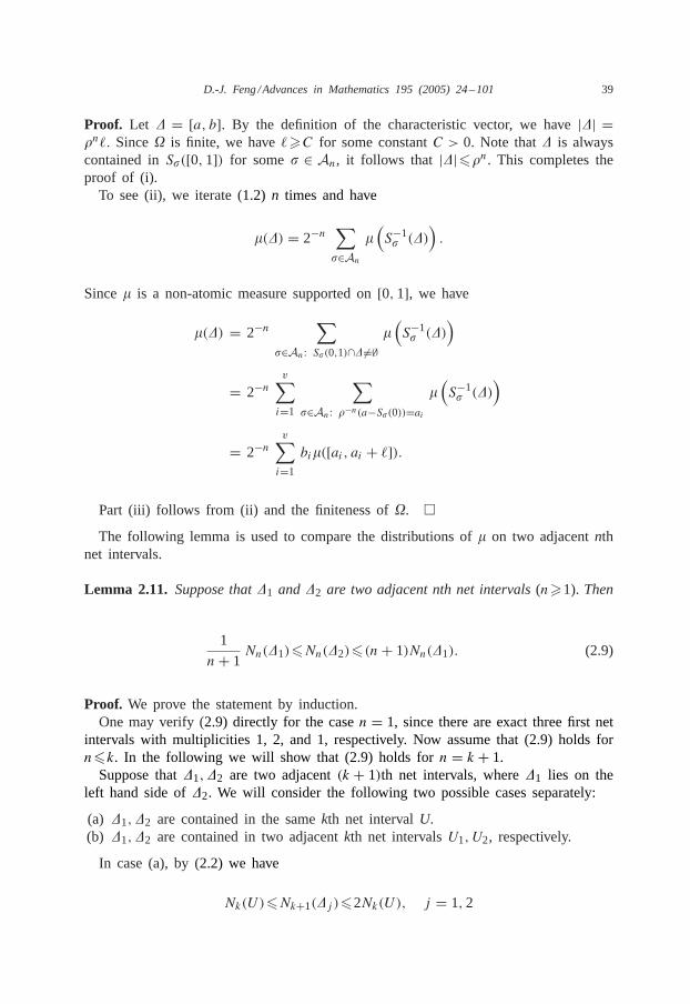
Part (iii) follows from (ii) and the finiteness of. �The following lemma is used to compare the distributions of� on two adjacentnth
net intervals.
Lemma 2.11. Suppose that�1 and�2 are two adjacent nth net intervals(n�1). Then
1
n+ 1Nn(�1)�Nn(�2)�(n+ 1)Nn(�1). (2.9)
Proof. We prove the statement by induction.One may verify (2.9) directly for the casen = 1, since there are exact three first net
intervals with multiplicities 1, 2, and 1, respectively. Now assume that (2.9) holds forn�k. In the following we will show that (2.9) holds forn = k + 1.Suppose that�1,�2 are two adjacent(k + 1)th net intervals, where�1 lies on the
left hand side of�2. We will consider the following two possible cases separately:
(a) �1,�2 are contained in the samekth net intervalU.(b) �1,�2 are contained in two adjacentkth net intervalsU1, U2, respectively.
In case (a), by (2.2) we have
Nk(U)�Nk+1(�j )�2Nk(U), j = 1,2

40 D.-J. Feng /Advances in Mathematics 195 (2005) 24–101
and thus12 Nk+1(�1)�Nk+1(�2)�2Nk+1(�1).
Therefore (2.9) holds for�1,�2 whenevern = k + 1.In case (b), let us define
D1 = {� ∈ Ak : S�([0,1]) ⊃ U1, and they share the same right end-point},D2 = {� ∈ Ak\D1 : S�([0,1]) ⊃ U1},D3 = {� ∈ Ak : S�([0,1]) ⊃ U2, and they share the same left end-point},D4 = {� ∈ Ak\D3 : S�([0,1]) ⊃ U2}.
From (2.2) and the definition of net interval, we have
D2 = D4,
Nk(U1) = #D1+ #D2, Nk(U2) = #D3+ #D4,
#D1+ #D2�Nk+1(�1)�#D1+ 2#D2,
#D3+ #A4�Nk+1(�2)�#D3+ 2#D4.
According to the above relations and the assumption
1
k + 1Nk(U1)�Nk(U2)�(k + 1)Nk(U1),
we have1
k + 2Nk+1(�1)�Nk+1(�2)�(k + 2)Nk+1(�1).
This completes the proof.�As a corollary of the above two lemmas, we have
Corollary 2.12. There exists a positive constant C such that
1nC
�(�1)��(�2)�nC�(�1), (2.10)
for any n�1 and any two adjacent nth net intervals�1, �2. Furthermore for a fixedpoint x ∈ [0,1],
limn→∞
log�([x − �n, x + �n])log�(In(x))
= 1,
whereIn(x) is an nth net interval containing x.

D.-J. Feng /Advances in Mathematics 195 (2005) 24–101 41
3. Fractal indices in terms of products of matrices
In this chapter we study some fractal indices about the Bernoulli convolution� andthe limited Rademacher functionf associated with a given Pisot reciprocal�. We willre-express those indices as the limits in terms of products of transition matrices.
3.1. Local dimensions of�
In this subsection we are concerned with the local dimensions of�. Recall that forany x ∈ [0,1], the local upper and lower dimensions of� at x, denoted asd(�, x) andd(�, x), respectively, are defined by
d(�, x) = lim supr→0
log�([x − r, x + r])logr
, d(�, x) = lim infr→0
log�([x − r, x + r])logr
.
A simple argument shows that
d(�, x) = lim supn→∞
log�([x − �n, x + �n])n log�
,
d(�, x) = lim infn→∞
log�([x − �n, x + �n])n log�
.
This combining Corollary2.12 yields
Lemma 3.1. For any x ∈ [0,1], we have
d(�, x) = lim supn→∞
log�(In(x))n log�
, d(�, x) = lim infn→∞
log�(In(x))n log�
,
whereIn(x) denotes an nth net interval containing x.
Let and A be constructed as in Section 2. Denote byNA the collection of all
admissible words of infinite length, i.e.,
NA =
{y = (yi)∞i=1 : yi ∈ , Ayi ,yi+1 = 1
}.
We use [�0] to denote the sub-collection of all admissible words of infinite lengthstarting from�0, the characteristic vector of the 0th net interval[0,1]. This is
[�0] = {y = (yi) ∈ NA : y1 = �0}.

42 D.-J. Feng /Advances in Mathematics 195 (2005) 24–101
There is a natural projection� from [�0] to the interval[0,1] defined by
�(y) =∞⋂n=1
�(y1 · · · yn+1), y = (yi), (3.1)
where�(y1 · · · yn+1) denote thenth net interval with the symbolic expressiony1 · · ·yn+1.Let {T (�, ), �, ∈ , A�, = 1} be the class of transition matrices given as in
Theorem2.9. Write for shortlyT�1�2···�n+1 := T (�1, �2) · · · T (�n, �n+1). Then we have
Theorem 3.2. For any y = (yi) ∈ [�0], we have
d(�,�(y)) = − log 2
log�+ lim sup
n→∞log‖Ty1···yn+1‖
n log�,
the lower dimensiond(�,�(y)) can be obtained by taking the lower limit.
Proof. Let x = �(y). Then �(y1 · · · yn+1) is an nth net interval containingx. ByTheorem2.9,
Nn(�(y1 · · · yn+1)) = ‖Wn(�(y1 · · · yn+1))‖ = ‖Ty1···yn+1‖.
Hence by Lemma2.10(iii), �(�(y1 · · · yn+1)) ≈ 2−n‖Ty1···yn+1‖. Using Lemma 3.1, weobtain the desired result.�
3.2. Lq -spectrum of�
In this subsection, we express theLq -spectrum of� as a limit in terms of productsof transition matrices.Recall for anyq ∈ R, theLq -spectrum�(q) of � is defined as
�(q) = lim inf�→0
log sup∑i �([xi − �, xi + �])q
log�,
where the superium is taken over all the families of disjoint intervals[xi − �, xi + �]with xi ∈ [0,1]. We will show that
Theorem 3.3. For any q ∈ R, we have
�(q) = −q log 2log�
+ lim infn→∞
log∑ ‖T�1···�n+1‖qn log�
, (3.2)
D.-J. Feng /Advances in Mathematics 195 (2005) 24–101 43
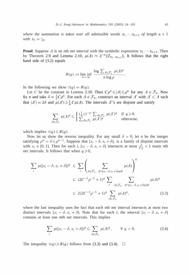
where the summation is taken over all admissible words�1 · · · �n+1 of length n + 1with �1 = �0.
Proof. Suppose� is annth net interval with the symbolic expression�1 · · · �n+1. Thenby Theorem2.9 and Lemma 2.10,�(�) ≈ 2−n‖T�1···�n+1‖. It follows that the righthand side of (3.2) equals
R(q) := lim infn→∞
log∑
�∈Fn �(�)q
n log�.
In the following we show�(q) = R(q).Let C be the constant in Lemma2.10. ThenC�n� |�|��n for any � ∈ Fn. Now
fix n and take� = 12C�n. For each� ∈ Fn, construct an interval�′ with �′ ⊂ � such
that |�′| = 2� and �(�′)� 14 C�(�). The intervals�′’s are disjoint and satisfy
∑�∈Fn
�(�)q�{(14 c)
−q ∑�∈Fn �(�′)q if q�0,∑
�∈Fn �(�′)q otherwise,
which implies�(q)�R(q).Now let us show the reverse inequality. For any small� > 0, let n be the integer
satisfying�n < ���n−1. Suppose that[xi − �, xi + �]i is a family of disjoint intervalswith xi ∈ [0,1]. Then for eachi, [xi − �, xi + �] intersects at most2
C� + 1 manynthnet intervals. It follows that whenq�0,
∑i
�([xi − �, xi + �])q �∑i
∑�∈Fn, �∩[xi−�,xi+�]�=∅
�(�)
q
� (2C−1�−1+ 1)q∑i
∑�∈Fn, �∩[xi−�,xi+�]�=∅
�(�)q
� 2(2C−1�−1+ 1)q∑
�∈Fn�(�)q, (3.3)
where the last inequality uses the fact that eachnth net interval intersects at most twodistinct intervals[xi − �, xi + �]. Note that for eachi, the interval [xi − �, xi + �]contains at least onemth net intervals. This implies
∑i
�([xi − �, xi + �])q�∑
�∈Fn�(�)q, ∀ q < 0. (3.4)
The inequality�(q)�R(q) follows from (3.3) and (3.4). �

44 D.-J. Feng /Advances in Mathematics 195 (2005) 24–101
3.3. The Hausdorff dimension of the graph of f
Let �(f ) denote the graph of the limited Rademacher functionf. In [53, p. 184],Przytycki and Urba´nski gave a formula of the Hausdorff dimension of�(f ), which isbased on the McMullen’s formula on the Hausdorff dimension of a class of self-affinesets [42,51]. Forn ∈ N, let an,1, . . . , an,sn (ranked in the increasing order) be all thedistinct points in{S�(0) : � ∈ An}. For j = 1, . . . , sn, denote by
dn,j = #{� ∈ An : S�(0) = an,j }.
The formula given by Przytycki and Urba´nski is just
dimH �(f ) = limn→∞
log∑snj=1(dn,j )− log�/ log 2
−n log�. (3.5)
Based on the above formula, we have
Theorem 3.4. The Hausdorff dimension of the graph of f satisfies
dimH �(f ) = limn→∞
log∑ ‖T�1···�n+1‖− log�/ log 2
−n log�, (3.6)
where the summation is taken over all admissible words�1 · · · �n+1 of length n + 1with �1 = �0.
Proof. Denoteu = − log�/ log 2. Then 0< u < 1. Set
m = sup{vn(�) : � ∈ Fn, n ∈ N},
where vn(�) is the dimension of the multiplicity vectorWn(�). By the finiteness of, we have 0< m <∞.Now fix n. Take� = [c, d] ∈ Fn. Write Wn(�) = (b1, . . . , bvn(�). Then we have
1
m
vn(�)∑i=1
bui �‖Wn(�)‖u�vn(�)∑i=1
bui . (3.7)
By the definition of multiplicity vector, the set{bi : 1� i�vn(�)} is equal to
⋃j : an,j∈(c−�n,c]
{dn,j }.

D.-J. Feng /Advances in Mathematics 195 (2005) 24–101 45
Therefore we have
1
m
∑j : an,j∈(c−�n,c]
dun,j�‖Wn(�)‖u�∑
j : an,j∈(c−�n,c]dun,j . (3.8)
Observe that for each 1�j < sn, there is at least one and at mostC−1 many distinct� = [c, d] ∈ Fn satisfying 0�c− an,j < �n, whereC is the constant in Lemma2.10.Taking the summation over� ∈ Fn in (3.8), we have
1
m
sn∑j=1
dun,j�∑
�∈Fn‖Wn(�)‖u�C−1
sn∑j=1
dun,j .
This combining (3.5) and Theorem 2.9 yields the desired result.�
3.4. The box dimension of the level sets of f
Recall that the level set off at t, denoted asLt , is defined by
Lt = {x ∈ [0,1] : f (x) = t}. (3.9)
Let the projection� : [�0] → [0,1] be defined as in (3.1). In this subsection we prove
Theorem 3.5. For any y = (yi)∞i=1 ∈ [�0], we have
dimB L�(y) = lim supn→∞
log‖Ty1...yn+1‖n log 2
,
dimB L�(y) = lim infn→∞
log‖Ty1...yn+1‖n log 2
.
wheredimB,dimB denote the upper and lower box dimension.
As a corollary of Theorems3.5 and 3.2, we have
Corollary 3.6. For any t ∈ [0,1], we have
dimB Lt = 1+ log�log 2
· d(�, t), dimB Lt = 1+ log�log 2
· d(�, t).
To prove Theorem3.5, we first give a lemma.

46 D.-J. Feng /Advances in Mathematics 195 (2005) 24–101
Lemma 3.7. For � = a1 · · · an∈An, let I� denote the nth2-adic interval[∑n
i=1 ai2−i ,∑ni=1 ai2−i + 2−n
). Then the image ofI� under f is the interval
J� :=[(1− �)
n∑i=1
ai�i−1, (1− �)n∑i=1
ai�i−1+ �n).
Proof. Recall that the Rademacher functionR is defined onR with period 1, takingvalues 0 and 1 on[0,1/2) and [1/2,1), respectively. Ifx ∈ I�, it can be checkeddirectly that
R(2i−1x) = ai, i = 1, . . . , n.
Therefore
f (x) = (1− �)∞∑i=1
R(2i−1x)�i−1
= (1− �)n∑i=1
ai�i−1+ (1− �)∞∑
j=n+1R(2j−1x)�j−1.
Hencef (x) ∈ J�.In the following we show that for anyt ∈ J�, there existsx ∈ I� such thatf (x) =
t . To prove this, setz = t1−� −
∑ni=1 ai�i−1. It is clear z ∈
[0, �n
1−�
)and t =
(1− �)(∑n
i=1 ai�i−1+ z). Let us consider the following�−1-expansion
z =∞∑
i=n+1ai�i−1, (3.10)
where the 0–1 coefficientsai (i�n+ 1) are defined by induction as follows:
an+1 ={1 if z��n,0 otherwise,
and if an+1, . . . , an+k are defined well, then
an+k+1 ={1 if z�(∑n+k
i=n+1 ai�i−1)+ �n+k,0 otherwise.
The sequence{ai}i�n+1 constructed as above satisfies the following property: for anym ∈ N, there isk > m such thatak = 0. Assume this is not true, i.e., there isk0 such
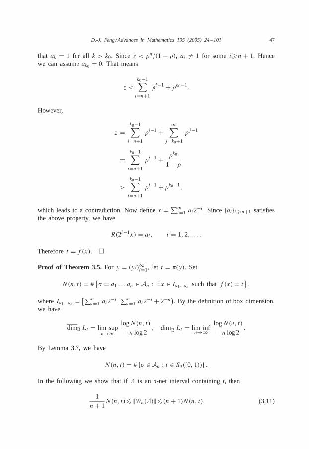
D.-J. Feng /Advances in Mathematics 195 (2005) 24–101 47
that ak = 1 for all k > k0. Sincez < �n/(1− �), ai �= 1 for somei�n + 1. Hencewe can assumeak0 = 0. That means
z <
k0−1∑i=n+1
�i−1+ �k0−1.
However,
z =k0−1∑i=n+1
�i−1+∞∑
j=k0+1�j−1
=k0−1∑i=n+1
�i−1+ �k0
1− �
>
k0−1∑i=n+1
�i−1+ �k0−1,
which leads to a contradiction. Now definex =∑∞i=1 ai2−i . Since{ai}i�n+1 satisfies
the above property, we have
R(2i−1x) = ai, i = 1,2, . . . .
Thereforet = f (x). �
Proof of Theorem 3.5.For y = (yi)∞i=1, let t = �(y). Set
N(n, t) = #{� = a1 . . . an ∈ An : ∃x ∈ Ia1...an such thatf (x) = t} ,
whereIa1...an =[∑n
i=1 ai2−i ,∑ni=1 ai2−i + 2−n
). By the definition of box dimension,
we have
dimB Lt = lim supn→∞
logN(n, t)
−n log 2 , dimB Lt = lim infn→∞
logN(n, t)
−n log 2 .
By Lemma3.7, we have
N(n, t) = # {� ∈ An : t ∈ S�([0,1))} .
In the following we show that if� is an n-net interval containingt, then
1
n+ 1N(n, t)�‖Wn(�)‖�(n+ 1)N(n, t). (3.11)

48 D.-J. Feng /Advances in Mathematics 195 (2005) 24–101
Table 2Elements in
� ∈ Labelled as
(1;0;1) 1(�;0;1) 2(1− �; (0,�);1) 3(�;1− �;1) 4(�; (0,1− �);1) 5(2�− 1;1− �;1) 6(1− �; (0,�);2) 7
In fact if t = 1, we may check directly thatN(n, t) = ‖Wn(�)‖ = 1 and thus (3.11)holds. Now we assumet ∈ [0,1). In this case, there is a uniquenth net interval�1 = [c, d] such thatt ∈ [c, d); furthermore for� ∈ An,
t ∈ S�([0,1))⇐⇒ 0�c − S�(0) < �n.
This implies that
‖Wn(�1)‖ = N(n, t).
However if �2 is anothernth interval containingt, then�2 and �1 are adjacent andthus by Lemma2.11,
1
n+ 1‖Wn(�1)‖�‖Wn(�2)‖�(n+ 1)‖Wn(�1)‖.
Hence (3.11) holds fort ∈ [0,1). By Theorem 2.9, we obtain the desired result.�
4. The golden ratio case
In this section we consider the concrete case� =√5−12 , the reciprocal of the golden
ratio.
4.1. The symbolic expressions and transition matrices
Let be the collection of all possible characteristic vectors. By a direct check (seeRemark 2.4) there are exact 7 elements in. We list them out Table 2.For our convenience, each element in is labelled by a digit from 1 to 7 as in the
above table. Especially, the characteristic vector(1;0;1) of the 0th net interval[0,1],is labelled as 1. Without confusion, we write directly
= {1,2, . . . ,7}. (4.1)

D.-J. Feng /Advances in Mathematics 195 (2005) 24–101 49
The transition map�, defined as in (2.7), is given by
�(1) = 234,
�(2) = 23,
�(3) = 5,
�(4) = 34,
�(5) = 367,
�(6) = 3,
�(7) = 5
and the 0–1 matrixA, which is induced by�, is the following:
A =
0 1 1 1 0 0 00 1 1 0 0 0 00 0 0 0 1 0 00 0 1 1 0 0 00 0 1 0 0 1 10 0 1 0 0 0 00 0 0 0 1 0 0
. (4.2)
The transition matricesT (i, j) constructed as in the proof of Lemma2.8, are listedas follows:
T (1,2) = 1, T (1,3) = [1,1], T (1,4) = 1,T (2,2) = 1, T (2,3) = [1,1],T (3,5) =
[1 00 1
],
T (4,3) = [1,1], T (4,4) = 1,
T (5,3) =[1 10 1
], T (5,6) =
[11
], T (5,7) =
[1 01 1
],
T (6,3) = [1,1],T (7,5) =
[1 00 1
].
(4.3)
For anyn�1, denote byA,n the collection of all admissible words of lengthn, i.e.,
A,n ={i1 . . . in ∈ ∗ : Aij ,ij+1 = 1, 1�j < n
},
where∗ denotes the collection of all finite words over. By Lemma2.7 and Theorem2.9, eachnth net interval� corresponds to a unique wordi1 . . . in+1 in A,n+1 with

50 D.-J. Feng /Advances in Mathematics 195 (2005) 24–101
i1 = 1; and the multiplicity vectorWn(�) satisfies
Wn(�) = Ti1...in+1 := T (i1, i2)T (i2, i3) . . . T (in, in+1).
To analyze the structure ofA,n, as well as the above products of matrices, wepresent the following simple but important fact:
Lemma 4.1. (i) := {3,5,6,7} is an essential subclass of. That is, { ∈ :A�, = 1} ⊂ for any � ∈ ; and for any�, ∈ , there exist�1, . . . , �n ∈ suchthat �1 = �, �n = and A�i ,�i+1 = 1 for 1� i�n− 1.(ii) The characteristic vector� = (2�− 1;1− �;1), represented by the symbol6 in
, satisfiesv(�) = 1.
For our convenience, denote byFn the collection of all admissible words of lengthn starting from 3, i.e.,
Fn = {i1 . . . in ∈ A,n : i1 = 3}.
By Lemma4.1, Fn ⊂ A,n.In the following we give the structure of the words inA,n, as well as the corre-
sponding products of matrices.
Lemma 4.2. For n�1, supposew = i1 . . . in+1 ∈ A,n+1 with i1 = 1. Then all thepossible forms of�, as well as‖T�‖, are the following:(1) � = 12. . .2︸ ︷︷ ︸
n
, and ‖T�‖ = 1.
(2) � = 14. . .4︸ ︷︷ ︸n
, and ‖T�‖ = 1.
(3) � = 12. . .2︸ ︷︷ ︸k
�, 0�k < n, � ∈ Fn−k, and ‖T�‖ = ‖T1�‖.(4) � = 14. . .4︸ ︷︷ ︸
k
�, 0�k < n, � ∈ Fn−k, and ‖T�‖ = ‖T1�‖.
Now set�0 = 3, �1 = 7 and
M0 =[1 10 1
], M1 =
[1 01 1
], M∅ =
[1 00 1
]. (4.4)
Write for simplicity Mi1...in = Mi1 . . .Min . Then we have
Lemma 4.3. Let � ∈ Fn for somen�1. Then all the possible forms of�, as well asthe value of‖T1�‖, are the following:(1) n = 1, � = 3. ‖T1�‖ = 2.

D.-J. Feng /Advances in Mathematics 195 (2005) 24–101 51
(2) n = 2, � = 35. ‖T1�‖ = 2.(3) n = 2k, k�2, � = 35 �i15 . . . �ik−15 with i1 . . . ik−1 ∈ Ak−1.
‖T1�‖ = ‖Mi1...ik−1‖.(4) n = 2k, k�2, � = 35 �i15 . . . �i&5 6�, where0�&�k − 2, i1 . . . i& ∈ A&,
� ∈ Fn−3−2&. ‖T1�‖ = ‖Mi1...i&‖ × ‖T1�‖.(5) n = 2k + 1, k�1, � = 35 �i15 . . . �ik−15 �ik , where i1 . . . ik ∈ Ak.
‖T1�‖ = ‖Mi1...ik‖.(6) n = 2k + 1, k�1, � = 35 �i15 . . . �ik−15 6, where i1 . . . ik−1 ∈ Ak−1.
‖T1�‖ = ‖Mi1...ik−1‖.(7) n = 2k + 1, k�2, � = 35 �i15 . . . �i&5 6�, where0�&�k − 2, i1 . . . i& ∈ A&,
� ∈ Fn−3−2&. ‖T1�‖ = ‖Mi1...i&‖ × ‖T1�‖.
4.2. The exponential sum of the products of transition matrices
In this subsection we determine the exact value of
E(q) := limn→∞
(∑‖Ti1...in+1‖q
)1/nfor any q ∈ R, where the summation is taken over all admissible wordsi1 . . . in+1 oflength n + 1 with i1 = 1. By Theorems3.3 and 3.4, this can be applied to calculatethe Lq -spectrum of� and the Hausdorff dimension of the graph off. We also checkthe differentiability ofE(q), which is necessary in the multifractal analysis of�.Let M0,M1 be defined as in (4.4). Forq ∈ R, defineu0(q) = 2q and
un(q) =∑J∈An
‖MJ ‖q, n = 1,2, . . . . (4.5)
The main result of this section is the following
Theorem 4.4. (i) For any q ∈ R, we haveE(q) = 1/x(q), where
x(q) = sup{x�0 :∞∑n=0
un(q)x2n+3�1}. (4.6)
(ii) There exists a uniqueq0 < −2 such that∞∑n=0
un(q0) = 1.Wheneverq > q0, x(q)
is the positive root of∞∑n=0
un(q)x2n+3 = 1, and it is an infinitely differentiable function
of q on (q0,+∞). Wheneverq�q0, x(q) = 1. Moreoverx(q) is not differentiable atq = q0.
We first consider part (i) of Theorem4.4. Forq ∈ R, define
Rn(q) =∑�∈Fn
‖T1�‖q, n�1,

52 D.-J. Feng /Advances in Mathematics 195 (2005) 24–101
where Fn denotes the collection all admissible words of lengthn starting from thesymbol 3. Set
R(q) = limn→∞ (Rn(q))
1/n .
By Lemma4.3, we have directly
Lemma 4.5. R1(q) = 2q = u0(q), R2(q) = 2q = u0(q), R3(q) = u0(q) + u1(q), andfor k�2,
R2k(q) =(k−2∑i=0
ui(q)R2k−2i−3(q))+ uk−1(q),
R2k+1(q) =(k−2∑i=0
ui(q)R2k+1−2i−3(q))+ uk−1(q)+ uk(q).
Now we prove
Lemma 4.6. R(q) = 1/x(q) for any q ∈ R.
Proof. We divide the proof into two steps.
Step1: lim supn→∞ (Rn(q))1/n �1/x(q). Since∞∑i=0
ui(q)x(q)3+2i�1, it follows that
for any k�1,
x(q)−2k �k∑i=0
ui(q)x(q)3+2i−2k
�k−2∑i=0
ui(q)x(q)3+2i−2k + uk−1(q)x(q) (4.7)
and similarly
x(q)−2k−1�k−2∑i=0
ui(q)x(q)3+2i−2k−1+ uk−1(q)+ uk(q)x(q)2. (4.8)
Choose a positive numberC > max{1, x(q)−2, x(q)−1} such that
Ri(q) < Cx(q)−i , i = 1,2,3.
We claim that
Ri(q) < Cx(q)−i (4.9)

D.-J. Feng /Advances in Mathematics 195 (2005) 24–101 53
for all i ∈ N. We show this claim by induction. Suppose (4.9) holds for anyi < 2k.By Lemma 4.5, (4.7) and (4.8), we have
R2k(q) =(k−2∑i=0
ui(q)R2k−2i−3(q))+ uk−1(q)
� C
(k−2∑i=0
ui(q)x(q)2i+3−2k
)+ uk−1(q)
� C
(k−2∑i=0
ui(q)x(q)2i+3−2k
)+ Cuk−1(q)x(q)
� Cx(q)−2k
and
R2k+1(q) =(k−2∑i=0
ui(q)R2k+1−2i−3(q))+ uk−1(q)+ uk(q)
� C
(k−2∑i=0
ui(q)x(q)2i+3−2k−1
)+ uk−1(q)+ uk(q)
� C
(k−2∑i=0
ui(q)x(q)2i+3−2k−1
)+ Cuk−1(q)+ Cuk(q)x(q)2
� Cx(q)−2k−1.
Therefore (4.9) holds fori = 2k and i = 2k + 1. This finishes the proof of the claim.Hence the main statement in this step follows.Step2: lim supn→∞ (Rn(q))1/n �1/x(q). To see this, take anyy ∈ (0, x(q)−1).
Sincey−1 > x(q), there exists a positive integerN such that
1<N−2∑i=0
ui,qy−3−2i .
Thus for k�N , we have
y2k�k−2∑i=0
ui(q)y2k−3−2i , y2k+1�
k−2∑i=0
ui(q)y2k+1−3−2i . (4.10)
Choose a positive numberD < min{1, x(q)−1, x(q)−2} such that
Ri(q) > Dyi, i = 1, . . . ,2N − 1.
54 D.-J. Feng /Advances in Mathematics 195 (2005) 24–101
Then by an argument similar to that in Step 1, we have
Ri(q) > Dyi, ∀i ∈ N,
which implies limm→∞
(Rn,q
)1/n �y. Since y ∈ (0,1/x(q)) is arbitrary, we obtain the
desired inequality in this step.�
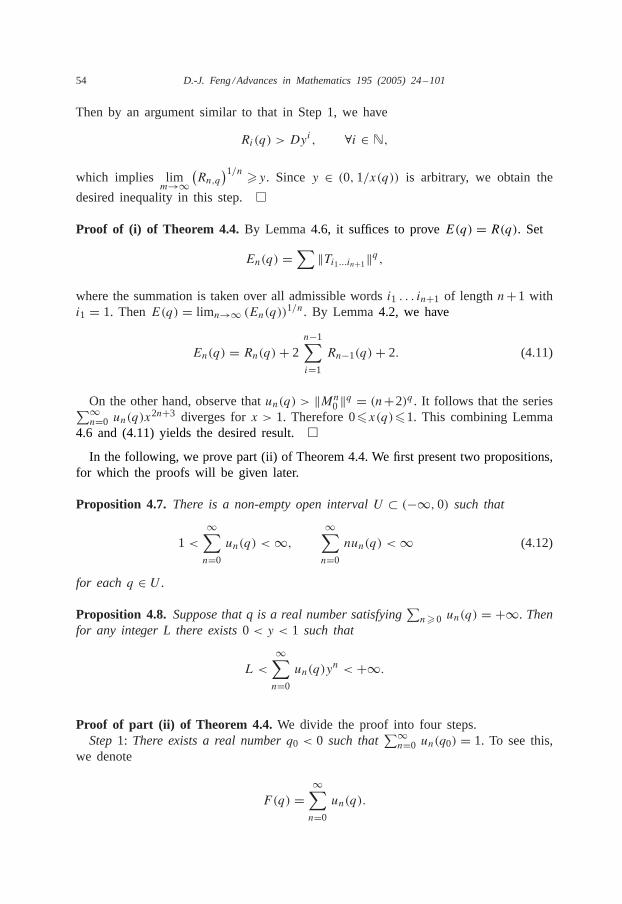
Proof of (i) of Theorem 4.4.By Lemma4.6, it suffices to proveE(q) = R(q). SetEn(q) =
∑‖Ti1...in+1‖q,
where the summation is taken over all admissible wordsi1 . . . in+1 of lengthn+1 withi1 = 1. ThenE(q) = limn→∞ (En(q))1/n. By Lemma4.2, we have
En(q) = Rn(q)+ 2n−1∑i=1
Rn−1(q)+ 2. (4.11)
On the other hand, observe thatun(q) > ‖Mn0‖q = (n+2)q . It follows that the series∑∞
n=0 un(q)x2n+3 diverges forx > 1. Therefore 0�x(q)�1. This combining Lemma4.6 and (4.11) yields the desired result.�In the following, we prove part (ii) of Theorem 4.4. We first present two propositions,
for which the proofs will be given later.
Proposition 4.7. There is a non-empty open intervalU ⊂ (−∞,0) such that
1<∞∑n=0
un(q) <∞,∞∑n=0
nun(q) <∞ (4.12)
for eachq ∈ U .
Proposition 4.8. Suppose that q is a real number satisfying∑n�0 un(q) = +∞. Then
for any integer L there exists0< y < 1 such that
L <
∞∑n=0
un(q)yn < +∞.
Proof of part (ii) of Theorem 4.4. We divide the proof into four steps.Step1: There exists a real numberq0 < 0 such that
∑∞n=0 un(q0) = 1. To see this,
we denote
F(q) =∞∑n=0
un(q).

D.-J. Feng /Advances in Mathematics 195 (2005) 24–101 55
By Proposition4.7, there existst < 0 such that 1< F(t) < ∞. Since un(q) isan increasing positive function ofq for each n, the series
∑∞n=1 un(q) converges
uniformly on (−∞, t). ThusF(q) is a continuous function on(−∞, t). The existenceof q0 follows from the Intermediate Value Theorem and the fact limq→−∞ F(q) = 0,which we will prove below.For anyn ∈ N and q < q ′ < t , we have
un(q)
un(q ′)� maxJ∈An
‖MJ ‖q−q ′�2q−q ′ ,
which impliesF(q)/F (q ′)�2q−q ′ and thus limq→−∞ F(q) = 0.Step2: Wheneverq�q0, x(q) = 1; and wheneverq > q0, x(q) is the positive root
of∑∞n=0 un(q)x2n+3 = 1. First assumeq�q0. In this case
∑∞n=0 un,q�1, and thus
x(q)�1. Sinceun(q) > ‖Mn0‖q = (n + 1)q , we have
∑n�0 un(q)x
2n+3 = ∞ forx > 1, which impliesx(q)�1. Thereforex(q) = 1.Now assumeq > q0. Under this assumption we have either
1<∞∑n=0
un(q) <∞
or∞∑n=0
un(q) = ∞.
In the first case,∑n�0 un(q)x
2n+3 is a continuous function ofx on (0,1) and thusthere existsy ∈ (0,1) satisfying∑∞
n=0 un(q)y2n+3 = 1, hencex(q) = y. In the secondcase, by Proposition4.8, there exists 0< t1 < t2 < 1 such that
1<∑n�0
un(q)t2n1 < +∞, t−31 <
∑n�0
un(q)t2n2 <∞.
Thus 1<∑∞n=0 un(q)t
2n+32 < ∞. Therefore
∑∞n=0 un(q)x2n+3 is a continuous func-
tion of x on (0, t2). Combining it with (4.6), we see thatx(q) satisfies∑∞n=0 un(q)
x(q)2n+3 = 1.Step3: x(q) is infinitely differentiable on(q0,+∞). Moreover
x′(q) = −∑∞n=0
(∑J∈An
‖MJ ‖q log‖MJ ‖)x(q)2n+3∑∞
n=0 un(q)(2n+ 3)x(q)2n+2, ∀ q > q0. (4.13)
To see it, define
F(q, x) =∞∑n=0
un(q)x2n+3.
56 D.-J. Feng /Advances in Mathematics 195 (2005) 24–101
Fix q1 ∈ (q0,+∞). As we have shown in step 2, there exists a real numbery > x(q1)
such that 1< F(q1, y) < +∞. Take a real numberz so thatx(q1) < z < y, and takeq2 such that
q2 > q1, 4q2−q1 < y
z.
Note that for any integern�0,
un(q2)
un(q1)� maxJ∈An
‖MJ ‖q2−q1�4n(q2−q1).
Therefore for anyq < q2 and 0< x < z, we have
F(q, x) �∞∑n=0
un(q2)z2n+3
�∞∑n=0
un(q1)y2n+34n(q2−q1)
(z
y
)2n+3< +∞,
∞∑n=0
dun(q)
dqx2n+3 =
∑n�0
( ∑J∈An
‖MJ ‖q log‖MJ ‖)x2n+3�
∞∑n=0
un(q)(log 4n)x2n+3
�∞∑n=0
un(q1)y2n+3(log 4n)4n(q2−q1)
(z
y
)2n+3< +∞
and
∞∑n=0
un(q)(3+ 2n)x2n+2 <∞∑n=0
un(q2)(3+ 2n)z2n+2
� 1
z
∞∑n=0
un(q1)y2n+3(3+ 2n)4n(q2−q1)
(z
y
)2n+3< +∞.
The above three inequalities imply thatF(q, x) is well defined and differentiable on(−∞, q2)× (0, z). Furthermore using similar discussions we can show thatF(q, x) isinfinitely differentiable on(−∞, q2)× (0, z). Thus by the Implicit Function Theorem,x(q) is infinitely differentiable on a neighborhood ofq1. Sinceq1 is taken arbitrarilyon (q0,+∞), x(q) is infinitely differentiable on(q0,+∞). Formula (4.13) follows bya direct calculation.

D.-J. Feng /Advances in Mathematics 195 (2005) 24–101 57
Step4: x(q) is not differentiable atq = q0. Note thatx′(q0−) = 0, we need toprove x′(q0+) < 0. To see it, notice that forq > q0,
∞∑n=0
un(q)x(q)2n+3−
∞∑n=0
un(q0)x(q0)2n+3 = 0.
Thus we have
x(q)− x(q0)q − q0 = −
∞∑n=0
un(q)− un(q0)q − q0 · x(q0)2n+3∑
n�0 un(q)(x(q)2n+2+ x(q)2n+1x(q0)+ · · · + x(q0)2n+2
)
= −
∞∑n=0
un(q)− un(q0)q − q0∑∞
n=0 un(q)(x(q)2n+2+ x(q)2n+1+ · · · + x(q)+ 1
) .Since
∑∞n=0 un(q)(2n+ 3) < +∞ on a neighborhood ofq0 (by Proposition4.7), we
obtain the following formula by takingq ↓ q0:
x′(q0+) = −∑n�0(
∑J∈An
‖MJ ‖q0 log‖MJ ‖)∑∞n=0 un(q0) · (2n+ 3)
< 0. �
In what follows, we give the proofs of Propositions4.7 and 4.8. First we givesome simple lemmas. For any positive integerk and positiven1, . . . , nk, we define forsimplicity
a(n1, . . . , nk) = (1,0)k∏i=0
(M�i
)ni (1,0)Tand
b(n1, . . . , nk) =∥∥∥∥∥k∏i=0
(M�i
)ni∥∥∥∥∥ ,where �i = 0 if i is odd, and�i = 1 if i is even.
Lemma 4.9. Let b(n1, . . . , nk) be defined as above, then
(i) b(n1, . . . , nk)�(1+ n1) . . . (1+ nk−1)(2+ nk).

58 D.-J. Feng /Advances in Mathematics 195 (2005) 24–101
(ii) b(n1, . . . , n2k)�(1+ n1n2) . . . (1+ n2k−1n2k) andb(n1, . . . , n2k+1)�(1+ n1n2) . . . (1+ n2k−1n2k)(1+ n2k+1).
Proof. Part (i) follows directly from the inequality
(1,1)Mn� �(n+ 1, n+ 1), � = 0 or 1.
To see part (ii), it suffices to notice that
(Mn10 M
n21 ) . . . (M
n2k−10 M
n2k1 ) =
(1+ n1n2 n1n2 1
). . .
(1+ n2k−1n2k n2k−1n2k 1
)�
((1+ n1n2) . . . (1+ n2k−1n2k) ∗
∗ ∗)
and
Mn10 M
n21 . . .M
n2k1 M
n2k+10 �
((1+ n1n2) . . . (1+ n2k−1n2k) ∗
∗ ∗)(
1 n2k+10 1
). �
Since any element in{0,1}n can be uniquely written as�n11 . . . �nkk , or (1−�1)n1 . . . (1−
�k)nk with n1+ · · · + nk = n, we obtain the following lemma immediately.
Lemma 4.10. For eachq ∈ R, we have
∞∑n=0
un(q) = 2q + 2∑n�1
b(n)q + 2∑l�2
∑n1,...,nl�1
b(n1, . . . , nl)q
= 2q + 2∑n�1
b(n)q + 2∑l�1
∑n1,...,n2l�1
b(n1, . . . , n2l )q
+2∑l�1
∑n1,...,n2l+1�1
b(n1, . . . , n2l+1)q
and
∞∑n=0
nun(q) = 2∑n�1
nb(n)q + 2∑l�1
∑n1,...,n2l�1
(n1+ · · · + n2l )b(n1, . . . , n2l )q
+2∑l�1
(n1+ · · · + n2l+1)∑
n1,...,n2l+1�1
b(n1, . . . , n2l+1)q .
D.-J. Feng /Advances in Mathematics 195 (2005) 24–101 59
Proof of Proposition 4.7.By Lemmas4.9 and 4.10, we have for anyq < 0,
∞∑n=0
un(q)
�2q + 2∑n�1
(2+ n)q + 2∑l�2
∑n1,...,nl�1
(1+ n1)q . . . (1+ nl−1)q(2+ nl)q
= 2q + 2
∑n�1
(2+ n)q1+∑
l�1
∑n�1
(1+ n)ql
(4.14)
and
∞∑n=0
nun(q)
�2∑n�1
n(2+ n)q + 2∑k�1
∑n1,...,n2k �1
(n1 + · · · + n2k)(1+ n1n2)q . . . (1+ n2k−1n2k)q
+ 2∑k�1
∑n1,...,n2k+1�1
(n1 + · · · + n2k+1)(1+ n1n2)q . . . (1+ n2k−1n2k)qnq2k+1
= 2∑n�1
n(2+ n)q + 2∑k�1
∑n1,...,n2k �1
2kn1(1+ n1n2)q . . . (1+ n2k−1n2k)q
+2∑k�1
∑n1,...,n2k+1�1
2kn1(1+ n1n2)q . . . (1+ n2k−1n2k)qnq2k+1
+2∑k�1
∑n1,...,n2k+1�1
n2k+1(1+ n1n2)q . . . (1+ n2k−1n2k)qnq2k+1
= 2∑n�1
n(2+ n)q +( ∑n1,n2�1
n1(1+ n1n2)q)( ∑
k�1
4k
( ∑m1,m2�1
(1+m1m2)q)k−1)
+( ∑n1,n2�1
n1(1+ n1n2)q)( ∑
n�1
nq)( ∑
k�1
4k
( ∑m1,m2�1
(1+m1m2)q)k−1)
+2
( ∑n�1
nq+1)( ∑
k�1
( ∑m1,m2�1
(1+m1m2)q)k)
.
(4.15)
By (4.14) and (4.15), to prove the proposition, it suffices to construct an intervalUsuch that for eachq ∈ U , one has∑n�1
nq+1 <∞,∑
n1,n2�1
n1(1+ n1n2)q <∞,∑
m1,m2�1
(1+m1m2)q < 1 (4.16)

60 D.-J. Feng /Advances in Mathematics 195 (2005) 24–101
and
2q + 2∑n�1
(2+ n)q + 2 ·(1+
∑n�1
nq)·(∑l�1
( ∑n1,n2�1
(1+ n1n2)q)l)
> 1. (4.17)
To do this, denote by� the Riemann–Zeta function, that is
�(x) =∑n�1
n−x, x > 1.
Let �0 be the positive root ofx2+ 2x − 98 = 0, i.e., �0 ≈ 0.45774. We set
U =(− �−1(1611),−�−1(1+ �0)
)≈ (−2.2599,−2.2543).
Now supposeq ∈ U . Sinceq < −2, we can see∑n�1 n
q+1 < ∞ and∑n1,n2�1
n1(1+ n1n2)q <∞. Moreover,∑n1,n2�1
(1+ n1n2)q = 2∑n�1
(1+ n)q − 2q +∑
n1,n2�2
(1+ n1n2)q
< 2∑n�1
(1+ n)q − 2q +∑n�2
nq
2
= 2(�(−q)− 1
)− 2q + (�(−q)− 1
)2< 2�0 − 1
8+ �20 = 1
and
2q + 2
∑n�1
(2+ n)q1+∑
l�1
∑n�1
(1+ n)ql
= 2q + 2 · �(−q)− 1− 2q
2− �(−q) = 1+ (3− 2q)�(−q)− 4
2− �(−q)
> 1+ (3− 2−2)�(−q)− 4
2− �(−q) > 1+ (3− 2−2) · 1611 − 4
2− �(−q) = 1.
Thus (4.16) and (4.17) hold whenq ∈ U , which completes the proof of theproposition. �

D.-J. Feng /Advances in Mathematics 195 (2005) 24–101 61
Proof of Proposition 4.8. First we assumeq > 0. In this case,un(q) > 1 for n�0,and therefore
∑n�0 un,q = +∞. Moreover, the sequence{un,q}n is sub-multiplicative,
this is um+n(q)�um(q)un(q). Thus
limn→+∞ un(q)
1/n = infn�1
un(q)1/n.
Denote byrq the value of above limit, then 1�rq < ∞ and un(q)�rnq for n�1.
Hence limx→r−1q
∞∑n=0
un(q)xn = +∞, which implies the desired result since the series∑∞
n=0 un(q)yn converges on(0, r−1q ).In the remaining part we assumeq < 0 and
∑∞n=0 un(q) = ∞. Note that for any
integersn1, n2, . . . , nl andm1,m2, . . . , ms , we have
a(n1, n2, . . . , nl)�b(n1, n2, . . . , nl)
and
a(n1, n2, . . . , nl)a(m1,m2, . . . , ms)�a(n1, n2, . . . , nl, m1,m2, . . . , ms), (4.18)
wherem1,m2, . . . , ms are positive integers. It is not hard to show that
a(n1, n2, . . . , nl)� 14 b(n1, n2, . . . , nl), if l is even. (4.19)
(To see this, denote (x1 x2x3 x4
)= (Mn1
0 Mn21 ) . . . (M
nl−10 M
nl1 )
for even integerl. Then by induction onl, one can verify that among thexi ’s, x1 isthe greatest andx4 the smallest.)For any integerL�1, take an integery(L)�L ·4−q and definep = 2y(L). Now for
any 0< x < 1,
∞∑n=0
un(q)xn
= 2q + 2 ·2p−1∑j=1
∑n1,...,nj �1
b(n1, n2, . . . , nj )q · xn1+···+nj
+2 ·2p−1∑j=0
+∞∑k=1
∑n1,...,n2kp+j �1
b(n1, . . . , n2kp+j )q · xn1+···+n2kp+j

62 D.-J. Feng /Advances in Mathematics 195 (2005) 24–101
�2q + 2 ·2p−1∑j=1
∑n1,...,nj �1
b(n1, n2, . . . , nj )q · xn1+···+nj
+2 ·2p−1∑j=0
+∞∑k=1
∑n1,...,n2kp+j �1
a(n1, . . . , n2kp+j )q · xn1+···+n2kp+j
�2q + 2 ·2p−1∑j=1
∑n1,...,nj �1
b(n1, n2, . . . , nj )q · xn1+···+nj
+2 ·2p−1∑j=0
+∞∑k=1
∑n1,...,n2kp+j �1
a(n1, . . . , n2kp)q
× a(n2kp+1, . . . , n2kp+j )qxn1+···+n2kp+j
�2q + 2 ·2p−1∑j=1
∑n1,...,nj �1
b(n1, n2, . . . , nj )q · xn1+···+nj
+2
2p−1∑j=0
∑n1,...,nj �1
a(n1, . . . , nj )q xn1+···+nj
× +∞∑k=1
∑n1,...,n2p�1
a(n1, . . . , n2p)q xn1+···+n2p
k . (4.20)
Sincea(n1, n2, . . . , nl), b(n1, n2, . . . , nl) are polynomials aboutn1, n2, . . . , nl and 0<x < 1, it follows
∑n1,...,nl�1
a(n1, . . . , nl)q xn1+···+nl <∞,
∑n1,...,nl�1
b(n1, . . . , nl)q xn1+···+nl <∞
for any positive integerl. Therefore by (4.20), we have
∑n�0
un(q)xn <∞
if∑n1,...,n2p�1 a(n1, . . . , n2p)
q xn1+···+n2p < 1.

D.-J. Feng /Advances in Mathematics 195 (2005) 24–101 63
Since∑∞n=0 un(q) = ∞, by (4.20) we have
∑n1,...,n2p�1
a(n1, . . . , n2p)q�1 or= +∞.
Hence there exists 0< z�1 such that∑n1,...,n2p�1
a(n1, . . . , n2p)qzn1+···+n2p = 1.
Moreover,
∞∑n=0
un(q)xn <∞, ∀x ∈ (0, z). (4.21)
For l = 2,22, . . . , p, by (4.18) we obtain
∑n1,...,n2p�1
a(n1, . . . , n2p)qzn1+···+n2p �
∑n1,...,nl�1
a(n1, . . . , nl)qzn1+···+nl
2p/l
,
which implies ∑n1,...,nl�1
a(n1, . . . , nl)qzn1+···+nl �1.
Thus by (4.19), we have∑n1,...,nl�1
b(n1, . . . , nl)qzn1+···+nl �4q, l = 2,22, . . . , p.
Therefore
limx→z−∑∞
n=0 un(q)xn
�2q + 2 ·∑2p−1
j=1∑
n1,...,nj �1b(n1, . . . , nj )
q · zn1+···+nj
�2q + 2 · y(L) · 4q�2q + 2L,
which finishes the proof. �
64 D.-J. Feng /Advances in Mathematics 195 (2005) 24–101
4.3. The Hausdorff dimension of the graph of f
Combining Theorems3.4 and 4.4, we have directly
Theorem 4.11.The Hausdorff dimension of the graph of f satisfies
dimH �(f ) = logx(− log�/ log 2)log�
,
wherex(− log�/ log 2) is the positive root of
∞∑n=0
∑J∈An
‖MJ ‖− log�/ log 2 x2n+3 = 1.
4.4. TheLq -spectrum of�
Combining Theorems3.3 and 4.4, we have directly
Theorem 4.12.For any q ∈ R, we have
�(q) = −q log 2log�
− logx(q)
log�,
wherex(q) satisfies(4.6). There exists a uniqueq0 < −2 such that∞∑n=0
∑J∈An
‖MJ ‖q0 = 1.
Wheneverq > q0, x(q) is the positive root of
∞∑n=0
∑J∈An
‖MJ ‖qx2n+3 = 1,
and it is an infinitely differentiable function of q on(q0,+∞). Wheneverq�q0,x(q) = 1. Moreoverx(q) is not differentiable atq = q0.
4.5. The Hausdorff dimension of�
The Hausdorff dimension of� has been considered by many authors (e.g. see[1,2,36,43,58]). A computable theoretical formula of dimH � was first given by Ledrap-pier and Porzio [36]. In this section, we state another theoretical formula obtained byNgai [43] based on the following result.

D.-J. Feng /Advances in Mathematics 195 (2005) 24–101 65
Theorem 4.13(Ngai [43] ). Suppose that� is a Borel probability measure onR withbounded support, and furthermore itsLq -spectrum�(�, q) is differentiable atq = 1.Then the local dimensiond(�, x) is equal to�′(�,1) for � almost all x ∈ R, and theHausdorff dimension of� is also equal to�′(�,1).
The above result has also been obtained (in a generalized form) by Heurteaux[23]and Olsen [45]. As we have showed in Theorem 4.12, theLq -spectrum�(q) of � isdifferentiable atq = 1. A direct calculation of�′(1) through the formula of�(q) givenin Theorem 4.12 yields
Theorem 4.14(Ngai [43] ). The Hausdorff dimension of� satisfies
dimH � = �′(1) = − log 2
log�+
∞∑n=0
2−2n−3∑J∈An
‖MJ ‖ log‖MJ ‖
9 log�.
In Remark4.26, we will provide another approach to the above formula.
4.6. Local dimensions of�
In this section we present results on the range and almost all value of the localdimensions of�. Recall thatd(�, x), d(�, x) and d(�, x) are used to denote the upperlocal dimension, the lower local dimension and local dimension, respectively, andR(�)the range ofd(�, x), i.e.,
R(�) := {y ∈ R : d(�, x) = y for somex ∈ [0,1]}.
The main results of this section are the following:
Theorem 4.15.R(�) =[− log 2
log�− 1
2, − log 2
log�
].
Theorem 4.16.For � almost all x ∈ [0,1],
d(�, x) = �′(1) = − log 2
log�+
∞∑n=0
2−2n−3∑J∈An
‖MJ ‖ log‖MJ ‖
9 log�.
Theorem 4.17.For L almost all x ∈ [0,1],
d(�, x) = − log 2
log�+ 7
√5− 15
10 log�·∞∑n=0
(3−√5
2
)n+1 ∑J∈An
log‖MJ ‖.

66 D.-J. Feng /Advances in Mathematics 195 (2005) 24–101
Theorem4.15 was first stated and proved by Hu [24]. In his proof, Hu used acomplicated combinatoric method. In this section we will give a new proof, which isalso valid to deal with the parameter�k (k = 3,4, . . .).Theorem 4.16 is just a combination of Ngai’s two results—Theorems 4.13 and 4.14.
Theorem 4.17 is new, and it can be used to determine the almost all value of the boxdimensions of level sets off. In what follows, we will prove Theorems 4.15 and 4.17,respectively.
Proof of Theorem 4.15.Denote
NA =
{(in)
∞n=1 : in ∈ , Ain,in+1 = 1 for n�1
},
where, A are defined as in (4.1) and (4.2). By Theorem 3.2, to determineR(�) itsuffices to determine the range, denoted asRT , of the limits
limn→∞
log‖Ti1...in+1‖n
,
where (in)∞n=1 ∈ NA with i1 = 1. Denote�0 = 3 and �1 = 7. Define a sequence of
sets(Bi )∞i=0 of admissible words by
B0 = {356},
Bn ={35�i15 . . . �in56 : i1 . . . in ∈ An
}, n = 1,2, . . .
and define
B =∞⋃n=0
Bn. (4.22)
It can be checked directly that 1�1 . . .�n is an admissible word starting from 1 forany �1, . . . ,�n ∈ B. Moreover, by Lemma4.3,
‖T1�1...�n‖ =n∏i=1‖T1�i‖.
Therefore we have
RT ⊃ [x0, y0]
with
x0 = inf�∈B
log‖T1�‖|�| , y0 = sup
�∈Blog‖T1�‖|�| ,
D.-J. Feng /Advances in Mathematics 195 (2005) 24–101 67
where |�| denotes the length of�. At the end of the proof, we will show that
x0 = 0, y0 = − log�2. (4.23)
Now we use (4.23) to prove
RT =[0, − log�
2
]. (4.24)
Observe that for eachn�1 and � = i1 . . . in+1 ∈ A,n+1 with i1 = 1, there exists aword �′ of length at most 3 such that��′ can be written as
1u&w1 . . .�m
with &,m�0, u = 2 or 4,�1, . . . ,�m ∈ B, and thus
T��′ =m∏i=1‖T1�i‖.
Hence we have
0� log‖Ti1...in+1‖n+ 3
�∑mi=1 log‖T1�i‖∑m
i=1 |�i |� − log�
2.
Letting n→∞, we obtainRT ⊂[0,− log�
2
]. Thus (4.24) holds and
R(�) =[− log 2
log�− 1
2, − log 2
log�
].
Now we turn to prove (4.23). Note that for eachn�1,
(35)n6 ∈ B, ‖T1(35)n6‖ = ‖Mn0‖ = n+ 2.
It follows that
infn
log‖T1(35)n6‖2n+ 1
= 0,
and thusx0 = 0.

68 D.-J. Feng /Advances in Mathematics 195 (2005) 24–101
On the other hand, for� = 35�i15 . . . �in56∈ Bn, we have
‖T1�‖ = ‖Mi1 . . .Min‖. (4.25)
Observe that
‖Mi1...in‖ < ‖M1−i1 . . .M1−ij−1M1−ijMij+1Mij+2 . . .Min‖
if ij = ij+1 for some 1�j < n. It follows that the maximum value of the right handside of (4.25) is attained wheni1, . . . , in take 0,1 alternatively. By a direct calculation,this maximum value is equal to
2+ �+ (−1)n�2n+41+ �2
�−n.
Therefore
y0 = supn�0
log(2+�+(−1)n�2n+4
1+�2 �−n)
2n+ 3
= supn�0
log(2+�+(−1)n�2n+4
1+�2
)+ log�−n
3+ 2n.
Since
1
3log
(2+ �+ (−1)n�2n+4
1+ �2
)� 1
3log
(2+ �+ �4
1+ �2
)= 1
3log 2
and
1
2nlog�−n = − log�
2,
we have
y0 = max
{log 2
3, − log�
2
}= − log�
2,
which finishes the proof. �
Proof of Theorem 4.17.For anyi ∈ = {1,2, . . . ,7}, denote by&i the relative length(i.e., the first term) of the characteristic vector labelled byi. By Table 4.1, we have
&1 = 1, &2 = &4 = &5 = �, &3 = &7 = 1− �, &6 = 2�− 1.

D.-J. Feng /Advances in Mathematics 195 (2005) 24–101 69
Denote = {3,5,6,7}. As we presented in Lemma4.1, is an essential subclass of
. Let(
NA ,�
)be a subshift space of finite type defined by
NA =
{(in)
∞n=1 : in ∈ , Ain,in+1 = 1 for n�1
},
and �((in)
∞n=1
) = (in+1)∞i=1. Especially define
[3] ={(in)
∞n=1 ∈
NA : i1 = 3
}.
For any� ∈ [3], it is clear 1� ∈ NA . Let � be the projection defined as in (3.1). We
define a map� : [3] → �(13) by
�(�) = �(1�), ∀� ∈ [3],
where�(13) denotes the 1st net interval with the symbolic expression 13. By a directcheck,�(13) = [1− �,�].Now we would like to define a Markov measure� on
NA , such that the measure
� ◦ �−1 on �(13) only differs from the Lebesgue measureL on �(13) by a constantfactor. Construct a matrixP = (Pi,j )i,j∈ by
Pi,j ={
�&j&i
if Ai,j = 1,0 otherwise.
One can check directly thatP is a primitive probability matrix. Letp = (pi)i∈ be theprobability vector satisfyingpP = p. A direct calculation shows that
p3 = �2�+1 = 5−√5
10 , p5 = 12�+1 =
√55 ,
p6 = 2�−12�+1 = 5−2√5
5 , p7 = 1−�2�+1 = 3
√5−510 .
Define� to be the(p, P ) Markov measure onNA , i.e.,� is the unique Borel probability
measure onNA satisfying
�([i1i2 . . . in]) = pi1Pi1,i2 . . . Pin−1,in
for any n�2 and any cylinder set
[i1i2 . . . in] :={(xj )
∞j=1 ∈
NA : xj = ij for 1�j�n
}.

70 D.-J. Feng /Advances in Mathematics 195 (2005) 24–101
The measure� is �-invariant and ergodic. The reader is referred to[59] for moreinformation about Markov measures. Now we claim that
� ◦ �−1(A) = p3
�&3L(A), ∀ Borel setA ⊂ �(13). (4.26)
To prove the claim, note that for anyi1 . . . in ∈ A,n with i1 = 3, the net interval�(1i1 . . . in) has the length�n&in , while
�([i1 . . . in]) = pi1Pi1,i2 . . . Pin−1,in = pi1n−1∏j=1
�&ij+1&ij
= pi1�n−1 &in
&i1= p3
�&3�n&in . (4.27)
It follows that (4.26) holds forA = �(1i1 . . . in). A standard argument using themonotone class theorem yields (4.26). Now we prove
limn→∞
log‖T1x1...xn‖n
=∑�∈B
�([6�]) log‖T1�‖ (4.28)
= 7√5− 15
10
∞∑n=0
(3−√5
2
)n+1 ∑J∈An
log‖MJ ‖ (4.29)
for � almost all (xj )∞j=1 ∈ [3], whereB is defined as in (4.22). To show this, define
E :={(xi)
∞i=1 ∈
NA : ∃ mj ↑ ∞, such that lim
j→∞mj
mj+1= 1, xmj = 6
}.
Since� is ergodic and�([6]) > 0, by the Birkhoff ergodic theorem we have�(E) = 1.Now for each� = (xi)
∞i=1 ∈ E ∩ [3], let mj = mj(�) (j ∈ N) be the increasing
sequence of all integersk satisfyingxk = 6. Write � as
� = �1 ◦ �2 ◦ . . . ◦ �n ◦ . . . ,
where�1 = (xi)m1i=1, �2 = (xi)
m2i=m1+1, . . . ,�n = (xi)
mni=mn−1+1, . . . . It is clear that
�i ∈ B for i�1. Furthermore,
‖T1�1...�n‖ =n∏i=1‖T1�i‖
= ‖T1�1‖ × ∏
�∈B, |�|�mn‖T1�‖
∑mn−|�|j=0 �[6�](�j�)
, (4.30)

D.-J. Feng /Advances in Mathematics 195 (2005) 24–101 71
where�[6�] denotes the characteristic function on[6�]. Hence
log‖T1�1...�n‖mn
= log‖T1�1‖mn
+∑
�∈B,|�|�mn
1
mn
mn−|�|∑j=0
�[6�](�j�) log‖T1�‖. (4.31)
Since� is ergodic, by the Birkhoff ergodic theorem, for each� ∈ B,
limn→∞
1
mn
mn−|�|∑j=0
�[6�](�j�) = �([6�]) (4.32)
for � almost all� ∈ E ∩ [3]. Combining (4.31) and (4.32) we obtain that
lim infn→∞
log‖T1�1...�n‖mn
�∑�∈B
�([6�]) log‖T1�‖ (4.33)
for � almost all� ∈ E ∩ [3]. Observe that‖T1�1...�n‖�4mn , thus the right hand sideof (4.33) converges with an upper bound log 4. To state the inequality for upper limits,we fix l ∈ N. For anyk > l and � = 35�i15 . . . �ik56∈ B, we have
‖T1�‖�‖T5�i15...�il 5‖ · ‖T5�i25...�il+15‖ . . . ‖T5�ik−l+15...�ik5‖.
Denote
Cl ={5�i1 . . . �il5 : i1 . . . il ∈ Al
}By (4.30), we have
log‖T1�1...�n‖mn
� log‖T1�1‖mn
+∑
�∈B,|�|�2l+3
1
mn
mn−|�|∑j=0
�[6�](�j�) log‖T1�‖
+∑�′∈Cl
1
mn
mn−2l∑j=0
�[�′](�j�) log‖T�′ ‖
whenevermn > 2l + 3. Thus by the Birkhoff ergodic theorem,
lim supn→∞
log‖T1�1...�n‖mn
�∑
�∈B, |�|�2l+3�([6�]) log‖T1�‖
+∑�′∈Cl
�([�′]) log‖T�′ ‖ (4.34)
72 D.-J. Feng /Advances in Mathematics 195 (2005) 24–101
for � almost all� ∈ E ∩ [3]. To estimate the second sum in (4.34), we observe thatfor each�′ = 5�i15 . . . �il5,
�([�′]) = p5P5,�i1P�i1,5
. . . P�il ,5
= p5
p3P3,5P�il ,5P5,6
· p3P3,5P5,�i1P�i1,5. . . P5,�il
P�il ,5P5,6
= p5
p3P3,5P�il ,5P5,6
�([35�i15 . . . �il56])
� max
{p5
p3P3,5P3,5P5,6,
p5
p3P3,5P7,5P5,6
}× �([35�i15 . . . �il56])
and
log‖T�′ ‖� log‖T135�i15...�il 56‖.
Hence
∑�′∈Cl
�([�′]) log‖T�′ ‖ � max
{p5
p3P3,5P3,5P5,6,
p5
p3p3,5P7,5P5,6
}
×∑
�∈B,|�|=2l+3�([�]) log‖T1�‖. (4.35)
Since∑
�∈B �([6�]) log‖T1�‖ converges and
�([6�]) = p6P6,3
p3�([�]), ∀ � ∈ B,
the right hand side of (4.35) tends to 0 asl →∞. Thus combining (4.33) and (4.34)we obtain
limn→∞
log‖T1�1...�n‖mn
=∑�∈B
�([6�]) log‖T1�‖
for � almost all� ∈ E ∩ [3]. Thus (4.28) holds from the facts limn→∞ mn+1mn
= 1 for� ∈ E ∩ [3] and �(E) = 1. Since for any� = 35�i15 . . . �in56∈ B,
�([6�]) = p6P6,3
p3�([�])
D.-J. Feng /Advances in Mathematics 195 (2005) 24–101 73
= p6P6,3
p3
p3
�&3�2n+3&6 (by (4.27))
= (2�− 1)�2n+3
2�+ 1
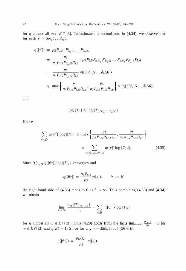
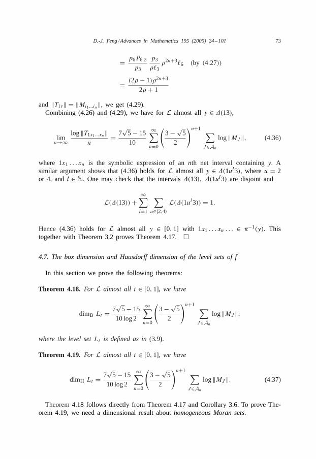
and ‖T1�‖ = ‖Mi1...in‖, we get (4.29).Combining (4.26) and (4.29), we have forL almost ally ∈ �(13),
limn→∞
log‖T1x1...xn‖n
= 7√5− 15
10
∞∑n=0
(3−√5
2
)n+1 ∑J∈An
log‖MJ ‖, (4.36)
where 1x1 . . . xn is the symbolic expression of annth net interval containingy. Asimilar argument shows that (4.36) holds forL almost ally ∈ �(1ul3), whereu = 2or 4, andl ∈ N. One may check that the intervals�(13), �(1ul3) are disjoint and
L(�(13))+∞∑l=1
∑u∈{2,4}
L(�(1ul3)) = 1.
Hence (4.36) holds forL almost all y ∈ [0,1] with 1x1 . . . xn . . . ∈ �−1(y). Thistogether with Theorem 3.2 proves Theorem 4.17.�
4.7. The box dimension and Hausdorff dimension of the level sets of f
In this section we prove the following theorems:
Theorem 4.18.For L almost all t ∈ [0,1], we have
dimB Lt = 7√5− 15
10 log 2
∞∑n=0
(3−√5
2
)n+1 ∑J∈An
log‖MJ ‖,
where the level setLt is defined as in(3.9).
Theorem 4.19.For L almost all t ∈ [0,1], we have
dimH Lt = 7√5− 15
10 log 2
∞∑n=0
(3−√5
2
)n+1 ∑J∈An
log‖MJ ‖. (4.37)
Theorem4.18 follows directly from Theorem 4.17 and Corollary 3.6. To prove The-orem 4.19, we need a dimensional result abouthomogeneous Moran sets.

74 D.-J. Feng /Advances in Mathematics 195 (2005) 24–101
Let {nk}k�1 be a sequence of positive integers and{ck}k�1 be a sequence of positivenumbers satisfyingnk�2, 0< ck < 1, n1c1�� and nkck�1 (k�2), where� is somepositive number. Let
D =⋃k�0
Dk with D0 = {∅}, Dk = {(i1, . . . , ik); 1� ij�nj , 1�j�k}.
If � = (�1, . . . , �k) ∈ Dk, � = (�1, . . . , �m) ∈ Dm, we define
� ∗ � = (�1, . . . , �k, �1, . . . , �m).
Suppose thatJ is an interval of length�. A collection F = {J� : � ∈ D} of subintervalsof J is said to have ahomogeneous Moran structureif it satisfies(1) J∅ = J ;(2) For any k�0 and � ∈ Dk, J�∗1, J�∗2, . . . , J�∗nk+1 are subintervals ofJ� and
J�∗i⋂J�∗j = ∅ (i �= j);
(3) For anyk�1 and any � ∈ Dk−1, 1�j�nk, we have
|J�∗j ||J�| = ck,
where |A| denotes the length ofA.If F is such a collection,F := ⋂
k�1
⋃�∈Dk
J� is called ahomogeneous Moran set
determined byF . We refer the readers to[19,21] for more information about homoge-neous Moran sets. For some applications of homogeneous Moran sets in the dimensiontheory of dynamical systems, see [10,11,17,50]. For the purpose of the present paper,we only need the following simplified version of a result contained in [21], whosesimpler proof was given in [10, Proposition 3].
Proposition 4.20. For the homogeneous Moran set F defined above, we have
dimH F� lim infn→∞
logn1n2 . . . nk− logc1c2 . . . ck+1nk+1
.
Proof of Theorem 4.19.We only prove (4.37) for L almost all t ∈ �(13). A similarargument can extend it forL almost all t ∈ �(1ul3) with u = 2 or 4, l�1.The upper bound is easy to see since we have always dimH Lt� dimB Lt . Now let
us consider the lower bound. We use some notations (the map�, the measure�, thecylinder set[3], the setE and the sequencemj = mj(�), etc.) introduced in the proofof Theorem 4.17. For any� ∈ E ∩ [3], write
� = �1 ◦ �2 ◦ . . .

D.-J. Feng /Advances in Mathematics 195 (2005) 24–101 75
with �i ∈ B. We claim that the level setL�(�) is a homogeneous Moran set withrespect tonk = ‖T1�k‖ and ck = 2−|�k |. Therefore by Proposition4.20,
dimH L�(�) � lim infk→∞
log(‖T1�1‖ × · · · × ‖T1�k‖)log(2|�1|+···+|�k+1| × ‖T1�k+1‖−1)
� lim infk→∞
log(‖T1�1‖ × · · · × ‖T1�k‖)log(2|�1|+···+|�k+1|)
= lim infk→∞
log(‖T1�1...�k‖)mk+1 log 2
= lim infk→∞
log(‖T1�1...�k‖)mk log 2
.
Combining it with (4.33), we obtain the lower bound of dimH L�(�) for � almost all� ∈ E ∩ [3]. By the equivalence of� andL, we get the lower bound of dimH Lt forL almost all t ∈ �(13).Now we prove the claim about the homogeneous Moran structure ofL�(�). For
k ∈ N, write �(1�1 . . .�mk ) = [ck, dk] and define
Dk :={a1 . . . amk ∈ Amk : �(1�) ∈ Ia1...amk
},
whereIa1...amk =[∑mk
i=1 ai2−i ,∑mki=1 ai2−i + 2mk
). By Lemma3.7,
Dk ={a1 . . . amk ∈ Amk : Sa1...amk ([0,1)) ⊃ [ck, dk)
}=
{a1 . . . amk ∈ Amk : 0�ck − Sa1...amk (0)��mk
}.
Observe that the characteristic vector of�(1�1 . . .�mk ), represented by the symbol6, is (2� − 1;1 − �;1). It follows that the pointsSa1...amk (0) are the same for alla1 . . . amk ∈ Amk . For � = a1 . . . amk ∈ Dk, define
J� =[mk∑i=1
ai2−i ,
mk∑i=1
ai2−i + 2mk
].
Then L�(1�) = ⋂∞k=1
⋃�∈Dk J� is a Moran set withnk = ‖T1�k‖ and ck = 2−|�k |.
This finishes the proof. �
4.8. The infinite similarity of�
We know that� is a self-similar measure generated by the similitudesS0 and S1(see (1.2)). However,Si (i = 1,2) have overlaps (i.e., they do not satisfy the open set

76 D.-J. Feng /Advances in Mathematics 195 (2005) 24–101
condition). In this section, we show that� is a locally infinitely generated self-similarmeasure without overlaps. More precisely, letB be defined as in (4.22), and denote
D ={1ul� : u = 2 or 4, l�0, � ∈ B
}.
It is clear that�� is an admissible word starting from the letter 1 for any� ∈ D and� ∈ B. Denote byg�,� the unique similitudecx + d with c > 0 so thatg�,�(�(�)) =�(��), where�(�) denotes the net interval with respect to the admissible word�.We have the following
Theorem 4.21.� is supported on⋃
�∈D �(�). For any fixed� ∈ D,
�� =∑�∈B
2−|�|‖T1�‖ · �� ◦ g−1�,�, (4.38)
where�� denotes the restriction of� on �(�), that is, ��(A) = �(A∩�(�)) for anyBorel setA ⊂ R. Furthermore,
g�,�(�(�)) = �(��) ⊂ �(�), �(��) ∩ �(��′) = ∅ f or � �= �′. (4.39)
To prove the above theorem, we need the following lemma.
Lemma 4.22. (i) �[1− �,�] = 13.
(ii)∑
�∈B �|�| = 1.(iii)
∑�∈B 2−|�|‖T1�‖ = 1.
Proof. By (1.2), we have
�(A) = 12 �
(S−10 (A)
)+ 1
2 �(S−11 (A)
)for any Borel setA ⊂ R. TakingA to be [0,1− �] and [�,1], respectively, we have
�([0,1− �]) = 12 �([0,1− �])+ 1
2 �([1− �,�])
and
�([�,1]) = 12 �([1− �,�])+ 1
2 �([�,1]).
These two equalities imply�([0,1− �]) = �([1− �,�]) = �([�,1]) = 13. Hence (i)
follows.

D.-J. Feng /Advances in Mathematics 195 (2005) 24–101 77
To see (ii), observe that each string inB is of length 3+ 2n (n�0), and for eachn�0 there are exact 2n different strings inB having length 3+ 2n. Therefore
∑�∈B
�|�| =∞∑n=0
2n�3+2n
= �3∞∑n=0(2�2)n = �3
1− 2�2= 1.
To see (iii), we have
∑�∈B
2−|�|‖T1�‖ = 2−3 · 2+∞∑n=1
∑i1...in∈An
2−3−2n(1,1)Mi1 . . .Min(1,1)T
= 2−2+∞∑n=1
2−3−2n(1,1)(M0 +M1)n(1,1)T
= 2−2+∑n�1
2−3−2n(1,1)[2 11 2
]n(1,1)T
= 2−2+∞∑n=1
2−3−2n · 2 · 3n
= 2−2+ 2−2∞∑n=1
(3
4
)n= 1. �
Proof of Theorem 4.21.It is not hard to see that the net intervals�(�) (� ∈ D) aredisjoint. Now we show that�
(⋃�∈D �(�)
) = 1. For each� ∈ B, by (ii) of Lemmas2.10 and 4.22 we have
�(�(1ul�)) = 2−|�|−l · ‖T1ul�‖ · �([1− �,�])= 2−|�|−l · ‖T1�‖ · �([1− �,�])= 1
3 · 2−|�|−l · ‖T1�‖, ∀u = 2 or 4, l�1.
Therefore
�
(⋃�∈D
�(�)
)=
∑�∈D
�(�(�))

78 D.-J. Feng /Advances in Mathematics 195 (2005) 24–101
=∑�∈B
1
3· 2−|�| · ‖T1�‖ + 2
∑�∈B
∞∑n=1
1
3· 2−|�|−n · ‖T1�‖
=∑�∈B
2−|�| · ‖T1�‖ = 1.
This is, � is supported on⋃
�∈D �(�). Similarly, we have
�
⋃�1,...,�n∈B
�(��1 . . . �n)
= �(�(�)), ∀ n ∈ N, � ∈ D.
For any �, �1, . . . , �n ∈ B, we claim thatg�,�(�(��1 . . . �n)) = �(���1 . . . �n). Tosee this, for two given intervals[a, b] and [c, d] with [a, b] ⊃ [c, d] we call the ratioc−ab−a the relative placeof [c, d] in [a, b]. Sinceg�,� is a similitude with positive ratio,the relative place ofg�,�(�(��1 . . . �n)) in g�,�(�(�)) = �(��) is the same as thatof �(��1 . . . �n) in �(�). To prove our claim, it suffices to show that the relativeplace of�(���1 . . . �n) in �(��) is the same as that of�(��1 . . . �n) in �(�), and thelength of g�,�(�(��1 . . . �n)) equals which of�(���1 . . . �n). The second fact is easyto see. Let us show the first one. By the structure of net intervals, the relative place of�(���1 . . . �n) in �(��) is determined completely by�1 . . . �n and the end letter of�,and the relative place of�(��1 . . . �n) in �(�) is determined completely by�1 . . . �nand the end letter of�. Since the end letter of� is the same as that of�, the firstfact follows.Now let us turn to prove (4.38) for a fixed� ∈ D. For n ∈ N and �1, . . . , �n ∈ B,
by the claim, we haveg�,�1(�(��2 . . . �n)) = �(��1 . . . �n). For � ∈ B and � �= �1, itis clear thatg�,�(�(�)) ∩ �(��1 . . . �n) = ∅ sinceg�,�(�(�)) = �(��). Therefore∑
�∈B2−|�|‖T1�‖ · �� ◦ g−1�,�(�(��1 . . . �n))
= 2−|�1|‖T1�1‖ · �� ◦ g−1�,�1(�(��1 . . . �n))
= 2−|�1|‖T1�1‖ · ��(�(��2 . . . �n))
= ��(�(��1 . . . �n)).
A standard argument using the monotone class yields (4.38).�
Remark 4.23. For each� ∈ D, �� is equivalent to a Bernoulli shift measure. To seethis, consider the one-side shift space(BN,�) over B. Endow this shift space with theproduct measure�, which satisfies
�([�]) = 2−|�|‖T1�‖, ∀� ∈ B.

D.-J. Feng /Advances in Mathematics 195 (2005) 24–101 79
Define the projection�� from BN to �(�) by
��((�n)∞n=1
) = ⋂n�1
�(��1 . . . �n).
Theorem4.21 implies that
� = 1
�(�(�))�� ◦ ��,
or equivalently,
�� = �(�(�)) · � ◦ �−1� .
4.9. The multifractal formalism for�
For ��0, defineK(�) = {x ∈ R : d(�, x) = �}. By Theorem4.15,
K(�) �= ∅ ⇐⇒ � ∈ R(�) =[− log 2
log�− 1
2,− log 2
log�
].
The main purpose of multifractal analysis is to study dimH K(�), which is calledthe multifractal spectrum of�. We refer the readers to the books[9,50] and papers[4,5,12,23,44,54] for more information about the multifractal analysis of measures. Inthis section, we prove
Theorem 4.24.Let q0 be defined as in Theorem4.4. Then for anyq �= q0, we have
dimH K(�(q)) = inft∈R{�(q)t − �(t)} = �(q)q − �(q), (4.40)
where�(t) is theLt -spectrum of�, and �(q) = �′(q).
Remark 4.25. Riedi and Mandelbrot[54] studied the multifractal structure of self-similar measures with infinitely many non-overlapping generators. They verified thevalidity of the multifractal formalism under some additional assumptions on the decayspeed of contraction ratios and probability weights (see [54, Theorem 10]). Howeverour measure� in Theorem 4.24 (and measures in Theorem 5.14) does not satisfy theirassumptions. By the way, the reader may see [40] for more details about dimensionsand measures in infinite iterated function systems.
Proof of Theorem 4.24.The upper bound
K(�)� inft∈R{�t − �(t)}, ∀� ∈ R(�)

80 D.-J. Feng /Advances in Mathematics 195 (2005) 24–101
is generic, not depending on the special property of� (see e.g.,[4, Theorem 1] or [32,Theorem 4.1]). In the following we prove the lower bound.First assumeq < q0. By Theorem 4.12,�(q) = − log 2
log� and −�(q) + �(q)q = 0.SinceK(�(q)) �= ∅, we have
dimH K(�(q))�0� inft∈R{�(q)t − �(t)}.
From now on, we assumeq > q0. Let B be defined as in (4.22). First we definea probability product measure�q on the shift space (BN,�) with the weightsp� =pq� r−�(q)� for each� ∈ B, where
p� = 2−|�|‖T1�‖, r� = �|�|.
Theorem4.12 implies∑
�∈B p� = 1. It is well known that�q is a �-invariant ergodicmeasure. Denote�0 = 356 and define the projection� = ��0 from BN to the netinterval V (1�0) by
�((�n)∞n=1
) = ∞⋂n=1
V (1�0�1 . . . �n).
The map� is continuous and injective (not surjective). Define
�q = �q ◦ �−1.
Then
�q(V (1�0�1 . . . �n)) = p�1 . . . p�n . (4.41)
Note that
�(V (1�0�1 . . . �n)) = �(V (1�0)) · p�1 . . . p�n , (4.42)
|V (1�0�1 . . . �n)| = |V (1�0)| · r�1 . . . r�n . (4.43)
Since �q is �-invariant and ergodic, by the Birkhoff ergodic theorem, there exists a
Borel measurable setGq ⊂ BN with �q(Gq) = 1 such that for each� = (�n)∞n=1 ∈ Gq ,
limn→∞
log�q(V (1�0�1 . . . �n))
n= limn→∞
1
n
n−1∑j=0
log p�j�|1

D.-J. Feng /Advances in Mathematics 195 (2005) 24–101 81
=∑�∈B
p� log p�
=∑�∈B
pq� r−�(q)� log
(p�r
−�(q)�
), (4.44)
limn→∞
log��(V (1�0�1 . . . �n))
n= limn→∞
1
n
n−1∑j=0
logp�j�|1
=∑�∈B
p� logp�
=∑�∈B
pq� r−�(q)� logp� (4.45)
and
limn→+∞
log |V (1�0�1 . . . �n)|n
= limn→+∞
1
n
n−1∑j=0
logr�j�|1
=∑�∈B
p� logr�
=∑�∈B
pq� r−�(q)� logr�, (4.46)
where�|1 = �1 for � = (�n)∞n=1 ∈ BN. The integrality of functions� %→ p�|1, � %→p�|1 and � %→ r�|1, or equivalently, the finiteness of
∑�∈B p
q� r−�(q)� log(p�r
−�(q)� ),∑
�∈B pq� r−�(q)� logp� and
∑�∈B p
q� r−�(q)� logr� come from the following inequality:
∞∑n=0
n∑J∈An
‖MJ ‖qx(q)2n+3 <∞, ∀q > q0
which was implied in Step 3 at the proof of part (ii) of Theorem4.4.Now fix � = (�n)∞n=1 ∈ Gq . By (4.43) we have
V (1�0�1 . . . �n) ⊂[�(�)− |V (1�0)| · r�1 . . . r�n , �(�)+ |V (1�0)| · r�1 . . . r�n
](4.47)
for all n ∈ N. On the other hand, we know that the end letter of the string�n+1 is 6.Changing from�n+1 this letter to 3 and 7, we get two wordsjn+1 and j ′n+1 respectively.The three net intervalsV (1�0�1 . . . �njn+1), V (1�0�1 . . . �n�n+1) andV (1�0�1 . . . �nj ′n+1)lie in V (1�0�1 . . . �n) in an increasing order with no overlaps. Furthermore, the first

82 D.-J. Feng /Advances in Mathematics 195 (2005) 24–101
and the third intervals have length larger than the second one. Therefore
V (1�0�1 . . . �n)
⊃ [�(�)− |V (1�0�1 . . . �n+1)|, �(�)+ |V (1�0�1 . . . �n+1)|
]= [�(�)− |V (1�0)| · r�1 . . . r�n+1, �(�)+ |V (1�0)| · r�1 . . . r�n+1] (4.48)
for all n ∈ N. Now for any small numberr > 0, choosen so that
|V (1�0)| · r�1 . . . r�nr�n+1�r < |V (1�0)| · r�1 . . . r�n .
By (4.47) and (4.48), we have
[�(�)− r,�(�)+ r]⊂ [
�(�)− |V (1�0)| · r�1 . . . r�n , �(�)+ |V (1�0)| · r�1 . . . r�n]
⊂ V (1�0�1 . . . �n−1), (4.49)
and
[�(�)− r,�(�)+ r]⊃ [
�(�)− |V (1�0)| · r�1 . . . r�n+1, �(�)+ |V (1�0)| · r�1 . . . r�n+1]
⊃ V (1�0�1 . . . �n+1). (4.50)
By (4.49), (4.50), and (4.44)–(4.46) and Theorem 4.4, we have
limn→∞
log�q [�(�)− r,�(�)+ r]logr
=∑
�∈B pq� r−�(q)� log(pq� r
−�(q)� )∑
�∈B pq� r−�(q)� logr�
= −�(q)+ �(q)q (4.51)
and
limn→+∞
log��[�(�)− r,�(�)+ r]logr
=∑
�∈B pq� r−�(q)� logp�∑
�∈B pq� r−�(q)� logr�
= �(q). (4.52)
Since�q(�(Gq)) = �q(Gq) = 1, by (4.51) we obtain
dimH �q = −�(q)+ �(q)q. (4.53)
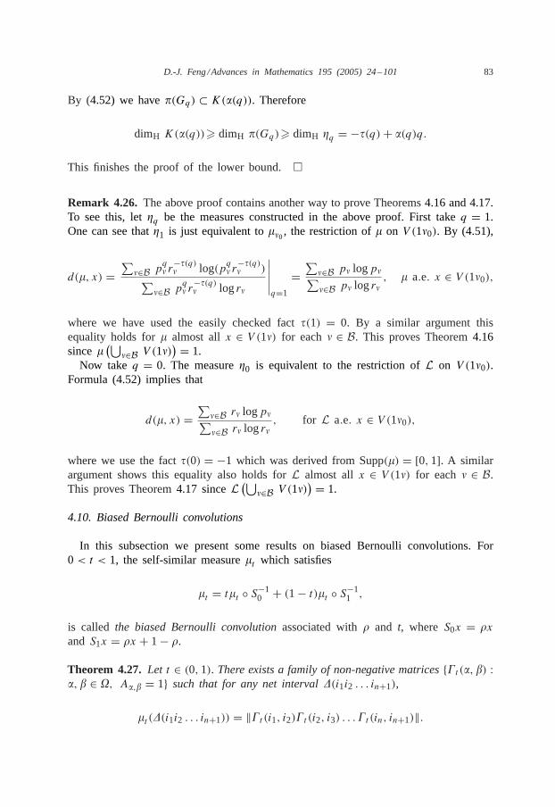
D.-J. Feng /Advances in Mathematics 195 (2005) 24–101 83
By (4.52) we have�(Gq) ⊂ K(�(q)). Therefore
dimH K(�(q))� dimH �(Gq)� dimH �q = −�(q)+ �(q)q.
This finishes the proof of the lower bound.�
Remark 4.26. The above proof contains another way to prove Theorems4.16 and 4.17.To see this, let�q be the measures constructed in the above proof. First takeq = 1.One can see that�1 is just equivalent to��0, the restriction of� on V (1�0). By (4.51),
d(�, x) =∑
�∈B pq� r−�(q)� log(pq� r
−�(q)� )∑
�∈B pq� r−�(q)� logr�
∣∣∣∣∣q=1
=∑
�∈B p� logp�∑�∈B p� logr�
, � a.e. x ∈ V (1�0),
where we have used the easily checked fact�(1) = 0. By a similar argument thisequality holds for� almost allx ∈ V (1�) for each� ∈ B. This proves Theorem4.16since�
(⋃�∈B V (1�)
) = 1.Now take q = 0. The measure�0 is equivalent to the restriction ofL on V (1�0).
Formula (4.52) implies that
d(�, x) =∑
�∈B r� logp�∑�∈B r� logr�
, for L a.e. x ∈ V (1�0),
where we use the fact�(0) = −1 which was derived from Supp(�) = [0,1]. A similarargument shows this equality also holds forL almost all x ∈ V (1�) for each� ∈ B.This proves Theorem4.17 sinceL (⋃
�∈B V (1�)) = 1.
4.10. Biased Bernoulli convolutions
In this subsection we present some results on biased Bernoulli convolutions. For0< t < 1, the self-similar measure�t which satisfies
�t = t�t ◦ S−10 + (1− t)�t ◦ S−11 ,
is called the biased Bernoulli convolutionassociated with� and t, whereS0x = �xand S1x = �x + 1− �.
Theorem 4.27.Let t ∈ (0,1). There exists a family of non-negative matrices{�t (�, ) :�, ∈ , A�, = 1} such that for any net interval�(i1i2 . . . in+1),
�t (�(i1i2 . . . in+1)) = ‖�t (i1, i2)�t (i2, i3) . . .�t (in, in+1)‖.

84 D.-J. Feng /Advances in Mathematics 195 (2005) 24–101
More precisely, these matrices are given by
�t (1,2) = t2
1−t+t2 , �t (1,3) =[t (1−t)21−t+t2 ,
t2(1−t)1−t+t2
], �t (1,4) = (1−t)2
1−t+t2 ,�t (2,2) = t, �t (2,3) = [(1− t)2, (1− t)t],�t (3,5) =
[1 00 1
],
�t (4,3) = [(1− t)t, t2], �t (4,4) = 1− t,�t (5,3) =
[t (1− t) t20 t2
], �t (5,6) =
[(1− t)t(1− t)t
], �t (5,7) =
[(1− t)2 0(1− t)2 (1− t)t
],
�t (6,3) = [1− t, t],�t (7,5) =
[1 00 1
].
Proof. The first part of the result was proved by the author under a more general setting(see[14, Theorem 3.3]). The second part involves the construction of these matrices�t (�, )’s, while the general method was given in the proof of [14, Lemma 3.2].�For any� = i1i2 . . . in ∈ B, define
pt,� = ‖�t (6, i1)�t (i1, i2)�t (i2, i3) . . .�t (in−1, in)‖.
Thenpt,� = [1− t, t]X∅[(1− t)t, (1− t)t]T for � = 356 and
pt,� = [1− t, t]Xi1 . . . Xin [(1− t)t, (1− t)t]T
for � = 35 �i15 . . . �in5 6, where�0 = 3, �1 = 7 and
X∅ =[1 00 1
], X0 =
[t (1− t) t20 t2
], X1 =
[(1− t)2 0(1− t)2 (1− t)t
]. (4.54)
It is easily checked that for any admissible word�� with � ∈ B,
�t (�(��)) = pt,��t (�(�)).
From the above equality we obtain an analogue of Theorem4.21:
Theorem 4.28.�t is supported on⋃
�∈D �(�). For any fixed� ∈ D,
�t,� =∑�∈B
pt,� · �t,� ◦ g−1�,�, (4.55)
where�t,� denotes the restriction of�t on �(�), i.e., ��(A) = �(A ∩ �(�)) for anyBorel setA ⊆ R.
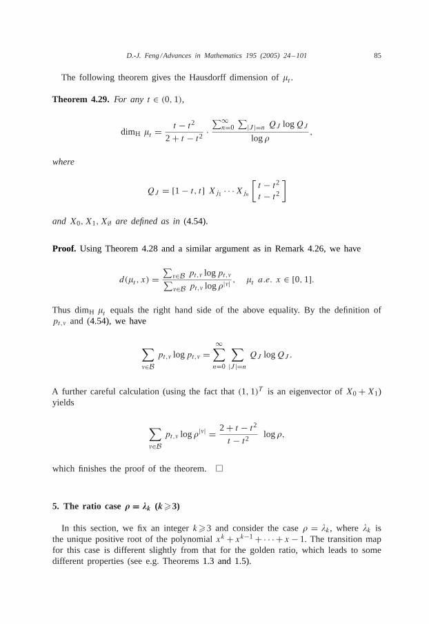
D.-J. Feng /Advances in Mathematics 195 (2005) 24–101 85
The following theorem gives the Hausdorff dimension of�t .
Theorem 4.29.For any t ∈ (0,1),
dimH �t =t − t2
2+ t − t2 ·∑∞n=0
∑|J |=n QJ logQJlog�
,
where
QJ = [1− t, t] Xj1 · · ·Xjn[t − t2t − t2
]
and X0, X1, X∅ are defined as in(4.54).
Proof. Using Theorem 4.28 and a similar argument as in Remark 4.26, we have
d(�t , x) =∑
�∈B pt,� logpt,�∑�∈B pt,� log�|�|
, �t a.e. x ∈ [0,1].
Thus dimH �t equals the right hand side of the above equality. By the definition ofpt,� and (4.54), we have
∑�∈B
pt,� logpt,� =∞∑n=0
∑|J |=n
QJ logQJ .
A further careful calculation (using the fact that(1,1)T is an eigenvector ofX0+X1)yields
∑�∈B
pt,� log�|�| = 2+ t − t2t − t2 log�,
which finishes the proof of the theorem.�
5. The ratio case� = �k (k�3)
In this section, we fix an integerk�3 and consider the case� = �k, where�k isthe unique positive root of the polynomialxk + xk−1+ · · · + x− 1. The transition mapfor this case is different slightly from that for the golden ratio, which leads to somedifferent properties (see e.g. Theorems1.3 and 1.5).

86 D.-J. Feng /Advances in Mathematics 195 (2005) 24–101
Table 3Elements in
� ∈ Labelled as
(1;0;1) a(1− �k;0;1) b(�k; (0,1− �k);1) c1(�k; (0,1− �k);2) c1(�k−i+1; (0,1− �k−i+1);1)
(i = 2,3, . . . , k)ci(i = 2,3, . . . , k)
(1− �k;�k;1) d(1− �k − �k−i ;�k;1)(i = 1,2, . . . , k − 1)
ei(i = 1,2, . . . , k − 1)
(1− �k − �k−i ;�k−i ;1)(i = 1,2, . . . , k − 1)
fi(i = 1,2, . . . , k − 1)
(1− 2�k;�k;1) g
5.1. The symbolic expressions and transition matrices
By an inductive discuss, we can determine all the elements in. In Table3 we listthem all, and for simplicity we relabel them by latin and arabic letters.The map�, defined as in (2.7), is given by
�(a) = b c1 d,
�(b) = b c1 e1,
�(c1) = c2,
�(c1) = c2,
�(ci) = ci+1 (i = 2, . . . , k − 1)
�(ck) = c1 g c1
�(d) = f1 c1 d,
�(ei) = f1 c1 ei+1 (i = 1, . . . , k − 2)
�(ek−1) = f1,
�(fi) = fi+1 c1 ei (i = 1, . . . , k − 2)
�(fk−1) = e1,
�(g) = f1 c1 e1
and the corresponding 0–1 matrixA = (Ai,j )i,j∈, is defined by
Ai,j ={1 if j is a letter of�(i),0 otherwise.
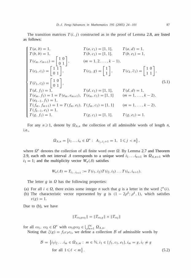
D.-J. Feng /Advances in Mathematics 195 (2005) 24–101 87
The transition matricesT (i, j) constructed as in the proof of Lemma2.8, are listedas follows:
T (a, b) = 1, T (a, c1) = [1,1], T (a, d) = 1,T (b, b) = 1, T (b, c1) = [1,1], T (b, e1) = 1,
T (cm, cm+1) =[1 00 1
], (m = 1,2, . . . , k − 1),
T (ck, c1) =[1 10 1
], T (ck, g) =
[11
], T (ck, c1) =
[1 01 1
],
T (c1, c2) =[1 00 1
],
T (d, f1) = 1, T (d, c1) = [1,1], T (d, d) = 1,T (em, f1) = 1= T (em, em+1), T (em, c1) = [1,1] (m = 1, . . . , k − 2),T (ek−1, f1) = 1,T (fm, fm+1) = 1= T (fm, e1), T (fm, c1) = [1,1] (m = 1, . . . , k − 2),T (fk−1, e1) = 1,T (g, f1) = 1, T (g, c1) = [1,1], T (g, e1) = 1.
(5.1)
For any n�1, denote byA,n the collection of all admissible words of lengthn,i.e.,
A,n ={i1 . . . in ∈ ∗ : Aij ,ij+1 = 1, 1�j < n
},
where∗ denotes the collection of all finite word over. By Lemma2.7 and Theorem2.9, eachnth net interval� corresponds to a unique wordi1 . . . in+1 in A,n+1 withi1 = 1; and the multiplicity vectorWn(�) satisfies
Wn(�) = Ti1...in+1 := T (i1, i2)T (i2, i3) . . . T (in, in+1).
The letterg in has the following properties:
(a) For all i ∈ , there exists some integern such thatg is a letter in the word�n(i).(b) The characteristic vector represented byg is (1 − 2�k;�k,1), which satisfies
v(g) = 1.
Due to (b), we have
‖T�1g�2‖ = ‖T�1g‖ × ‖T�2‖
for all �1, �2 ∈ ∗ with �1g�2 ∈⋃∞n=1 A,n.
Noting that�(g) = f1c1e1, we define a collectionB of admissible words by
B = {i1i2 . . . im ∈ A,m : m ∈ N, i1 ∈ {f1, c1, e1}, im = g, i& �= gfor all 1�& < m
}. (5.2)

88 D.-J. Feng /Advances in Mathematics 195 (2005) 24–101
To describe the structure ofB, we define:
B0 := c1c2 . . . ck,
B1 := c1c2 . . . ck,
Y(j)0 := e1 . . . ej (j = 1, . . . , k − 1),
Y(j)1 := f1 . . . fj (j = 1, . . . , k − 1).
From the form of�, we can check that
Lemma 5.1. A word � ∈ B if and only if it has one of the following forms:
(1) � = Bi1 . . . Bi&g, where& ∈ N, i1, . . . , i& ∈ {0,1} and i1 = 0.
(2) � = Y (p1)i1. . . Y
(pm)im
�, where � is of form (1), m ∈ N, 1�p1, . . . , pm−1�k − 1,
1�pm�k − 2, is = 1−(−1)s2 (s = 1, . . . , m) or is = 1+(−1)s
2 (s = 1, . . . , m).
Furthermore if� has the form(1), then
‖T�‖ ={2 f or & = 1,‖Mi2...i&‖ f or &�2;
and if � has the form(2), then ‖T�‖ = ‖T�‖.
In the following lemma, we list some basic facts which can be derived from theform of � and properties (a) and (b):
Lemma 5.2. (i) := \{a, b, d} is an essential subclass of. The characteristicvector � = (1− 2�k;�k;1), represented by the symbol g in, satisfiesv(�) = 1.(ii) For any word� in A,n, there exists a word� ∈⋃k+2
j=1 A,j with the end letterg such that�� ∈ A,n+|�| and ‖T��‖ = ‖T�‖ or 2‖T�‖.(iii) Let � be any word in
⋃∞n=1 A,n with first letter a. Then one can find a word
� ∈⋃k+1n=1 A,n such that the word�� has one of the following three forms:
1. �� = a�1 . . .�&, the first letter of�1 is c12. �� = a b . . . b︸ ︷︷ ︸
r
�1 . . .�&, the first letter of�1 is c1 or e1
3. �� = a d . . . d︸ ︷︷ ︸r
�1 . . .�&, the first letter of�1 is c1 or f1
where&, r ∈ N and �i ∈ B for 1� i�&.(iv) For any �1, . . . ,�& ∈ B,
�1 · · ·�& ∈∞⋃n=1
A,n, and ‖T�1···�&‖ =&∏i=1‖T�i‖ =
&∏i=1‖Tg�i‖.

D.-J. Feng /Advances in Mathematics 195 (2005) 24–101 89
5.2. The exponential sum of the product of matrices
In this subsection we will determine the value of
E(q) := limn→∞
(∑‖Ti1...in+1‖q
)1/nfor any q ∈ R, where the summation is taken over all admissible wordsi1 . . . in+1 oflength n+ 1 with i1 = a. More precisely, we prove the following:
Theorem 5.3. For any q ∈ R, E(q) = 1/x(q), wherex(q) is the unique positive rootof
1− 2xk−1+ xk1− 2x + xk ·
∞∑n=0
un(q)xkn+k+1 = 1 (5.3)
which lies in the interval(0, �k−1). Here un(q) is defined as in(4.5). Furthermore,x(q) is an infinitely differentiable function of q onR.
To prove the theorem, denote byFn the collection of all admissible words of lengthn starting from a letter in{c1, e1, f1}, i.e.,
Fn ={i1 . . . in ∈ A,n : i1 ∈ {c1, e1, f1}
}.
For q ∈ R, define
Rn(q) =∑�∈Fn
‖Tg�‖q, n�1.
Set
R(q) = limn→∞ (Rn(q))
1/n .
We first determine the value ofR(q). To achieve this, we define
wn(q) =∑
�∈B,|�|=n‖Tg�‖q, n ∈ N, q ∈ R. (5.4)
Lemma 5.4. For any n�2, we have
Rn(q) = on(q)+n∑i=1
wi(q)Rn−i (q),
whereon(q) is a number in(0, 2|q|
∑k+2i=1 wn+i (q)
).

90 D.-J. Feng /Advances in Mathematics 195 (2005) 24–101
Proof. Partition Fn into its two subsetsF (1)n and F (2)n , where F (1)n consists of allthe words inFn which do not contain the letterg and F (2)n = Fn\F (1)n . By Lemma5.2(ii), each word� ∈ F (1)n can be extended to a word inB by attaching some word� ∈⋃k+2
j=1 A,j with ‖T�‖�‖T��‖�2‖T�‖. This implies
∑�∈F (1)n
‖Tg�‖q�2|q|k+2∑i=1
wn+i (q). (5.5)
Observe that each word inF (2)n can be uniquely written as�� for some� ∈ B and� ∈ Fn−|�|. This deduces
∑�∈F (2)n
‖Tg�‖q =n∑i=1
wi(q)Rn−i (q). (5.6)
Combining (5.6) with (5.5) yields the desired result.�According the above lemma, using an argument similar to that in the proof of Lemma
4.6, we have
Lemma 5.5. R(q) = 1/x(q) for any q ∈ R, wherex(q) is defined by
x(q) ={x�0 :
∞∑n=1
wn(q)xn�1
}. (5.7)
To study the value ofx(q) in the above lemma, we define a sequence of integers{tn}∞n=0 by letting t0 = 1 and 1
2 tn (n > 0) be the number of different integral solutionsof the following conditional Diophantine equation:
p1+ · · · + pm = n with m ∈ N, 1�p1, . . . , pm−1�k − 1, 1�pm�k − 2.
Lemma 5.6. (i) For any positive integer n,
tn = 2 · (1,1, . . . ,1︸ ︷︷ ︸k−2
,0) ·
1 1 · · · 1 11 0 · · · 0 00 1 · · · 0 0....... . .......
0 0 · · · 1 0
n−1
100...
0
.
(ii) For any x�0,
1+∞∑n=1
tnxn =
1− 2xk−1+ xk1− 2x + xk if 0�x < �k−1,
+∞ if x��k−1.(5.8)

D.-J. Feng /Advances in Mathematics 195 (2005) 24–101 91
Proof. Denote by12 t(i)n (1� i�k−1) the number of integral solutions of the following
conditional equation:
p1+ · · · + pm = n, with m ∈ N, 1�p1, . . . , pm−1�k − 1, pm = i.
Then t (1)1 = 2 and t (i)1 = 0 for 2� i�k − 1. Furthermore for anyn�1,
{t(1)n+1 =
∑k−1i=1 t
(i)n ,
t(j)n+1 = t (j−1)n (j = 2, . . . , k − 1).
(5.9)
Hence we have
(t (1)n , t
(2)n , . . . , t
(k−1)n
)T = Qn−1(2,0, . . . ,0)T ,whereQ denotes the matrix in the formula fortn. Observingtn = ∑k−2
i=1 t(i)n , we get
the desired formula fortn.To prove (ii), define a sequence{sn}∞n=1 by s1 = s2 = · · · = sk−2 = 0, sk−1 = 1
and
sn = sn−1+ sn−2+ · · · + sn−k−1, ∀n�k.
Denotep(x) =∑∞n=1 snxn. Then
p(x) =k−1∑i=1
sixi +
∞∑n=k(sn−1+ sn−2+ · · · + sn−k+1)xn
= xk−1+k−1∑i=1
xi
( ∞∑n=k−i
snxn
)
= xk−1+(k−1∑i=1
xi
)p(x).
This deduces
p(x) ={
xk−11−∑k−1
i=1 xiif 0�x < �k−1,
+∞ for x��k−1.

92 D.-J. Feng /Advances in Mathematics 195 (2005) 24–101
By the definition ofsn we haveQn−1(1,0, . . . ,0)T = (sn+k−2, sn+k−3, . . . , sn)T . Hencetn = 2
∑k−2i=1 sn+i . Therefore
1+∞∑n=1
tnxn = 1+ 2
k−2∑i=1
∞∑n=1
sn+ixn
= 1+ 2k−2∑i=1
x−i∞∑
n=i+1snx
n
= 1+ 2p(x)k−2∑i=1
x−i .
Combining the above result with the expression ofp(x), we obtain the formula in (ii)directly. �Now we give the exact expression ofx(q).
Proposition 5.7. Let x(q) be defined as in(5.7) and un(q) defined as in(4.5). Thenfor any q ∈ R, x(q) is the unique positive root of
1− 2xk−1+ xk1− 2x + xk ·
∞∑n=0
un(q)xkn+k+1 = 1 (5.10)
which lies in the interval(0, �k−1). Furthermore, x(q) is an infinitely differentiablefunction of q onR.
Proof. By Lemma5.1 and the definition ofwn(q) (see (5.4)), we have
wn(q) ={0 for 1�n < k + 1,∑i,j�0: i+kj+k+1=n tiuj (q) for n�k + 1.
Therefore
∞∑n=1
wn(q)xn =
∞∑i=0
∞∑j=0
tiuj (q)xi+kj+k+1
=(1+
∞∑i=1
tixi
)·( ∞∑n=0
un(q)xkn+k+1
), (5.11)
where 1+∑∞i=1 tixi can be simplified as in (5.8).
To prove thatx(q) satisfies (5.10) and is differentiable infinitely, as that in the proofof Theorem 4.4(ii), essentially we only need to show that for anyq ∈ R, there exists

D.-J. Feng /Advances in Mathematics 195 (2005) 24–101 93
0 < y < 1 such that 1<∑∞n=1 wn(q)yn < ∞. Assume this fact is not true. Then
there existq ′ ∈ R and 0< x′ < 1 such that∑∞n=1 wn(q ′)(x′)n�1 and
∞∑n=1
wn(q′)zn = +∞, ∀z > x′. (5.12)
By (5.11) and∑∞n=1 wn(q ′)(x′)n�1, we have
x′ ∈ (0, �k−1) and∞∑n=0
un(q′) (x′)kn+k+1 < +∞.
Thus by (5.11) and (5.12), we have
∞∑n=0
un(q′)zkn+k+1 = +∞ ∀z > x′, (5.13)
which implies∑∞n=0 un(q ′) = +∞ since x′ < 1. Therefore by Proposition4.8, there
exists 0< y < 1 such that
∞∑n=0
un(q′) (x′)kn <
∞∑n=0
un(q′) ykn < +∞,
which leads to a contradiction with (5.13). This finishes the proof of the proposition.�
Proof of Theorem 5.3.By Lemma 5.5 and Proposition 5.7, to prove Theorem 5.3 weonly need to showE(q) = R(q) for q ∈ R. Define
En(q) =∑
‖Ti1...in+1‖q,
where the summation is taken over for all wordsi1 . . . in+1 in A,n+1 with i1 = a.Take�0 = B0g. Then for any� ∈ Fn−k−2, a�0� ∈ A,n+1. Therefore for anyn�k+3,
En(q) �∑
�∈Fn−k−2‖Ta�0�‖q
=∑
�∈Fn−k−2‖Tg�‖q = Rn−k−2(q).

94 D.-J. Feng /Advances in Mathematics 195 (2005) 24–101
On the other hand, by Lemma5.2(iii) each word inA,n+1 with the first lettera hasone of the following forms
a� (� ∈ Fn); abm� (� ∈ Fn−m); adm� (� ∈ Fn−m).
Hence,
En(q) �∑�∈Fn
‖Ta�‖q +n∑m=1
∑�∈Fn−m
‖Tabm�‖q +n∑m=1
∑�∈Fn−m
‖Tadm�‖q
= Rn(q)+ 2n∑m=1
Rn−m(q).
Using the above two inequalities and the factR(q)�1, we haveE(q) = R(q). Thisproves the theorem.�
5.3. The Hausdorff dimension of the graph f, theLq -spectrum and Hausdorffdimension of�
The main result of this subsection is the following:
Theorem 5.8. Let x(q) be given as in Theorem5.3. Then
(i) The Hausdorff dimension of the graph of f satisfies
dimH �(f ) = logx(− log�/ log 2)log�
.
(ii) For any q ∈ R, the Lq -spectrum�(q) of � satisfies
�(q) = −q log 2log�
− logx(q)
log�.
Furthermore�(q) is infinitely differentiable onR.(iii) The Hausdorff dimension of� is
dimH � = − log 2
log�+(2k − 3
2k − 1
)2
·
∞∑n=0
2−kn−k−1∑J∈An
‖MJ ‖ log‖MJ ‖
log�.
Proof. Combining Theorem3.4 with Theorem 5.3 yields (i) directly. Similarly, com-bining Theorem 3.3 with Theorem 5.3 yields (ii). To show (iii), by Theorem 4.14,
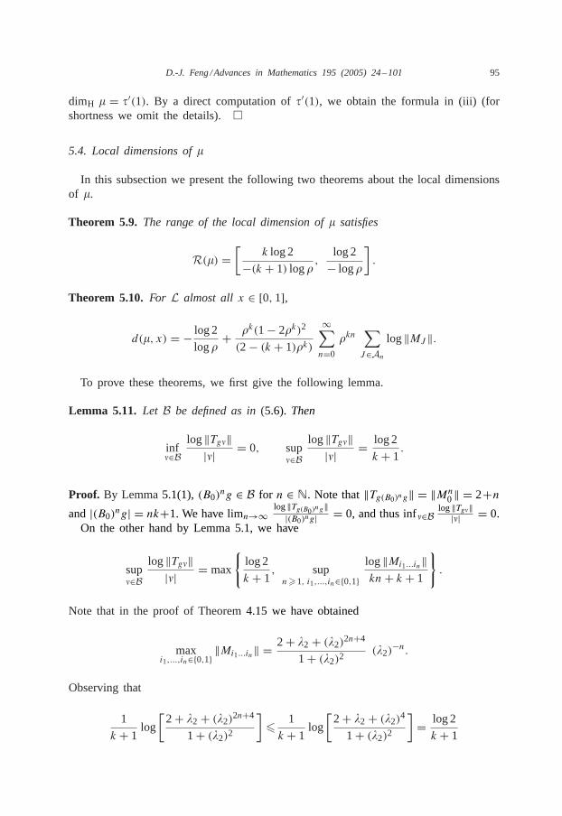
D.-J. Feng /Advances in Mathematics 195 (2005) 24–101 95
dimH � = �′(1). By a direct computation of�′(1), we obtain the formula in (iii) (forshortness we omit the details).�
5.4. Local dimensions of�
In this subsection we present the following two theorems about the local dimensionsof �.
Theorem 5.9. The range of the local dimension of� satisfies
R(�) =[
k log 2
−(k + 1) log�,
log 2
− log�
].
Theorem 5.10.For L almost all x ∈ [0,1],
d(�, x) = − log 2
log�+ �k(1− 2�k)2
(2− (k + 1)�k)
∞∑n=0
�kn∑J∈An
log‖MJ ‖.
To prove these theorems, we first give the following lemma.
Lemma 5.11. Let B be defined as in(5.6). Then
inf�∈B
log‖Tg�‖|�| = 0, sup
�∈Blog‖Tg�‖|�| = log 2
k + 1.
Proof. By Lemma5.1(1),(B0)ng ∈ B for n ∈ N. Note that‖Tg(B0)ng‖ = ‖Mn0‖ = 2+n
and|(B0)ng| = nk+1. We have limn→∞log‖Tg(B0)ng‖|(B0)ng| = 0, and thus inf�∈B
log‖Tg�‖|�| = 0.
On the other hand by Lemma 5.1, we have
sup�∈B
log‖Tg�‖|�| = max
{log 2
k + 1, supn�1, i1,...,in∈{0,1}
log‖Mi1...in‖kn+ k + 1
}.
Note that in the proof of Theorem4.15 we have obtained
maxi1,...,in∈{0,1}
‖Mi1...in‖ =2+ �2+ (�2)2n+4
1+ (�2)2 (�2)−n.
Observing that
1
k + 1log
[2+ �2+ (�2)2n+4
1+ (�2)2]
� 1
k + 1log
[2+ �2+ (�2)41+ (�2)2
]= log 2
k + 1

96 D.-J. Feng /Advances in Mathematics 195 (2005) 24–101
and
log(�2)−n
nk= − log�2
k<
log 2
k + 1,
we have
supn�1, i1,...,in∈{0,1}
log‖Mi1...in‖kn+ k + 1
� log 2
k + 1,
where we have used the inequalitya+cb+d � max{ a
b, cd} for positive numbersa, b, c, d.
Therefore sup�∈Blog‖Tg�‖|�| = log 2
k+1 . This finishes the proof of the lemma.�
Proof of Theorem 5.9.Using an argument similar to that in the proof of Theorem
4.15, we can prove thatR(�) =[− log 2
log� + 1log� sup�∈B
log‖Tg�‖|�| , − log 2
log� + 1log� inf �∈B
log‖Tg�‖|�|
]. Combining it with Lemma 5.11 yields the theorem.�
Proof of Theorem 5.10. Let = \{a, b, d}. Consider the one-sided shift space(
NA ,�
), where
NA =
{(in)
∞n=1 : in ∈ , Ain,in+1 = 1 for n�1
},
and �((in)
∞n=1
) = (in+1)∞i=1.Define a probability matrixP = (
Pi,j)i,j∈ by
Pi,j ={
� &j&i
if Ai,j = 1,0 otherwise,
where &i denotes the relative length of the characteristic vector labelled byi. Letp =(pi)i∈ be the probability vector such thatp = pP . By a careful calculation, wehave
pg = �k(1− 2�k)2− (k + 1)�k
, pc2 = · · · = pck−1 = �k
2−(k+1)�k ,
pc1 = (1−�k)�k
2−(k+1)�k , pei = pfi = �i (1−�k−�k−i )2−(k+1)�k (i = 1, . . . , k − 1),
pc1 = �2k
2−(k+1)�k .

D.-J. Feng /Advances in Mathematics 195 (2005) 24–101 97
Define � to be the (p, P ) Markov measure onNA . Using the Birkhoff ergodic
theorem and a proof essentially identical to that of Theorem4.17, we have
limn→∞
log‖Tx1...xn‖n
=∑�∈B
�([g�]) log‖Tg�‖
for � almost allx = (xj )∞j=1 ∈ NA , where[i1 . . . in] denote then-cylinder set
{(xj )
∞j=1 ∈
NA : xj = ij for 1�j�n
}.
Furthermore forL almost allx ∈ [0,1],
d(�, x) = − log 2
log�+ 1
log�
∑�∈B
�([g�]) log‖Tg�‖.
Now we are going to compute∑
�∈B �([g�]) log‖Tg�‖. By the definition of�, we have
�([i1 . . . in]) = pi1n−1∏j=1
�&ij+1&ij
= �n−1 pi1&in&i1
.
Thus for each� ∈ B, we have�([g�]) = �|�|pg. By Lemma5.1 and (5.8), we have∑�∈B
�([g�]) log‖Tg�‖ =∑�∈B
pg�|�| log‖Tg�‖
= pg
∞∑i=0
∞∑j=0
�i+kj+k+1ti∑J∈Aj
log‖MJ ‖
= pg�k+11− 2�k−1+ �k
1− 2�+ �k
∞∑j=0
�kj∑J∈Aj
log‖MJ ‖
= �k(1− 2�k)2
(2− (k + 1)�k)
∞∑j=0
�kj∑J∈Aj
log‖MJ ‖.
This finishes the proof of the theorem.�
5.5. The box dimension and Hausdorff dimension of�
In this subsection we prove

98 D.-J. Feng /Advances in Mathematics 195 (2005) 24–101
Theorem 5.12.For L almost all t ∈ [0,1], the Hausdorff dimension and box-countingdimension of t-level set of the limit Rademacher function f with parameter� = �k areequal to
�k(1− 2�k
)2(2− (k + 1)�k
)log 2
∞∑n=0
�kn∑J∈An
log‖MJ ‖
Proof. The result for the box-counting dimension follows directly from Corollary3.6and Theorem 5.10. The proof for the coincidence of the Hausdorff dimension and thebox-counting dimension for almost allt is essentially identical to that of Theorem 4.19by using the dimensional result about homogeneous Moran sets.�
5.6. The infinite similarity and multifractal formalism for�
Denote
D = {i1i2 . . . in ∈ A,n : n ∈ N, i1 = a, in = g, ij �= g for 1�j < n
}.
For any� ∈ D and � ∈ B, denote by��,� the unique similitudecx + d with c > 0so that��,�(�(�)) = �(��), where�(�) denotes the net interval with respect to theadmissible word�. Then the following theorem can be proved in the same line as thatof Theorem4.21:
Theorem 5.13.� is supported on⋃
�∈D �(�). For any fixed� ∈ D,
�� =∑�∈B
2−|�|‖Tg�‖ · �� ◦ �−1�,�, (5.14)
where �� denotes the restriction of� on �(�), i.e., ��(A) = �(A ∩ �(�)) for anyBorel setA ⊂ R. Furthermore,
��,�(�(�)) = �(��) ⊂ �(�), �(��) ∩ �(��′) = ∅ f or � �= �′. (5.15)
Using the above theorem and a proof identical to that in Theorem4.24, we have
Theorem 5.14.Then for anyq ∈ R, we have
dimH K�(q) = inft∈R{�(q)t − �(t)} = �(q)q − �(q), (5.16)
whereK(�) = {x ∈ R : d(�, x) = �}, �(t) is theLt -spectrum of�, and �(q) = �′(q).

D.-J. Feng /Advances in Mathematics 195 (2005) 24–101 99
Remark 5.15. After our work, Olivier et al.[46] also verifies the validity of the mul-tifractal formalism for� by viewing � as a weak Gibbs measure.
Acknowledgments
The main results of this paper were announced earlier in [13]. The author thanksProf. Zhi-Ying Wen, Prof. Yang Wang and Dr. Jun Wu for some helpful discussions. Hethanks Prof. Ka-Sing Lau for his careful reading of an earlier version of the manuscriptand many suggestions that led to the improvement of the manuscript.
References
[1] J.C. Alexander, J.A. Yorke, Fat baker’s transformations, Ergodic Theory Dyn. Systems 4 (1984)1–23.
[2] J.C. Alexander, D. Zagier, The entropy of a certain infinitely convolved Bernoulli measure, J. LondonMath. Soc. (2) 44 (1991) 121–134.
[3] M.J. Bertin, A. Decomps-Guilloux, M. Grandet-Hugot, M. Pathiaux-Delefosse, J.P. Schreiber, Pisotand Salem Numbers, Birkhäuser, Basel, 1992.
[4] G. Brown, G. Michon, J. Peyrière, On the multifractal analysis of measures, J. Statist. Phys. 66(1992) 775–790.
[5] R. Cawley, R.D. Mauldin, Multifractal decompositions of Moran fractals, Adv. Math. 92 (1992)196–236.
[6] P. Erdös, On a family of symmetric Bernoulli convolutions, Amer. J. Math. 61 (1939) 974–976.[7] P. Erdös, On the smoothness properties of a families of Bernoulli convolutions, Amer. J. Math. 62
(1940) 180–186.[8] K.J. Falconer, Fractal Geometry, Mathematical Foundations and Applications, Wiley, New York, 1990.[9] K.J. Falconer, Techniques in Fractal Geometry, Wiley, Chichester, 1997.[10] A.H. Fan, D.J. Feng, On the distribution of long-term time averages on symbolic space, J. Statist.
Phys. 99 (2000) 813–856.[11] A.H. Fan, D.J. Feng, J. Wu, Recurrence, dimension and entropy, J. London Math. Soc. (2) 64 (2001)
229–244.[12] A.H. Fan, K.S. Lau, S.M. Ngai, Iterated function systems without overlaps, Asian J. Math. 4 (2000)
527–552.[13] D.J. Feng, On the limit Rademacher functions and Bernoulli convolutions, in: Dynamical Systems,
Proceedings of the International Conference in Honor of Professor Liao Shantao, World Scientific,Singapore, 1999, pp. 46–49.
[14] D.J. Feng, The smoothness ofLq -spectrum of self-similar measures with overlaps, J. Lond. Math.Soc. 68 (2) (2003) 102–118.
[15] D.J. Feng, K.S. Lau, The pressure function for products of non-negative matrices, Math. Res. Lett.9 (2002) 363–378.
[16] D.J. Feng, K.S. Lau, X.Y. Wang, Some exceptional phenomena in multifractal formalism: Part II,preprint.
[17] D.J. Feng, K.S. Lau, J. Wu, Ergodic limits on the conformal repellers, Adv. Math. 169 (2002)58–91.
[18] D.J. Feng, E. Olivier, Multifractal analysis of the weak Gibbs measures and phase transition-applications to some Bernoulli convolutions, Ergodic Theory Dyn. Systems 23 (2003) 1751–1784.
[19] D.J. Feng, H. Rao, J. Wu, The measure properties of symmetric Cantor sets and their applications,Progr. Natur. Sci. 7 (1997) 172–178 (English Ed.).
[20] D.J. Feng, Y. Wang, Bernoulli convolutions associated with certain non-Pisot numbers, Adv. Math.187 (2004) 173–194.

100 D.-J. Feng /Advances in Mathematics 195 (2005) 24–101
[21] D.J. Feng, Z.Y. Wen, J. Wu, Some dimensional results for homogeneous Moran sets, Sci. China Ser.A 40 (1997) 475–482.
[22] A.M. Garsia, Arithmetic properties of Bernoulli convolutions, Trans. Amer. Math. Soc. 102 (1962)409–432.
[23] Y. Heurteaux, Estimations de la dimension inférieure et de la dimension supérieure des mesures,Ann. Inst. H. Poincaré Probab. Statist. 34 (1998) 309–338.
[24] T.Y. Hu, The local dimensions of the Bernoulli convolution associated with the golden number,Trans. Amer. Math. Soc. 349 (1997) 2917–2940.
[25] T.Y. Hu, K.S. Lau, The sums of Rademacher functions and Hausdorff dimension, Math. Proc.Cambridge Philos. Soc. 108 (1990) 97–103.
[26] T.Y. Hu, K.S. Lau, Hausdorff dimension of the level sets of Rademacher series, Bull. Polish Acad.Sci. Math. 41 (1993) 11–18.
[27] J.E. Hutchinson, Fractals and self-similarity, Indiana Univ. Math. J. 30 (1981) 713–747.[28] B. Jessen, A. Wintner, Distribution functions and the Riemann zeta function, Trans. Amer. Math.
Soc. 38 (1935) 48–88.[29] S.P. Lalley, Random series in powers of algebraic integers: Hausdorff dimension of the limit
distribution, J. London Math. Soc. 57 (2) (1998) 629–654.[30] K.S. Lau, Iterated function systems with overlaps and multifractal structure, in: Proceedings of
Trends in Probability and Related Analysis (Taipei, 1998), World Scientific, River Edge, NJ, 1999,pp. 35–76.
[31] K.S. Lau, Fractal measures and meanp-variations, J. Funct. Anal. 108 (1992) 427–457.[32] K.S. Lau, S.M. Ngai, Multifractal measure and a weak separation condition, Adv. Math. 141 (1999)
45–96.[33] K.S. Lau, S.M. Ngai, TheLq -dimension of the Bernoulli convolution associated with the golden
number, Studia Math. 131 (1998) 225–251.[34] K.S. Lau, S.M. Ngai, TheLq -dimension of the Bernoulli convolution associated with P. V. numbers,
Osaka J. Math. 36 (1999) 993–1010.[35] K.S. Lau, X.Y. Wang, Some exceptional phenomena in multifractal formalism: Part I, preprint.[36] F. Ledrappier, A. Porzio, A dimension formula for Bernoulli convolutions, J. Statist. Phys. 76 (1994)
1307–1327.[37] F. Ledrappier, A. Porzio, On the multifractal analysis of Bernoulli convolutions, I. Large-deviation
results, II. Dimensions, J. Statist. Phys. 82 (1996) 367–420.[38] P. Mattila, Geometry of Sets and Measures in Euclidean Spaces, Cambridge University Press,
Cambridge, 1995.[39] R.D. Mauldin, K. Simon, The equivalence of some Bernoulli convolutions to Lebesgue measure,
Proc. Amer. Math. Soc. 126 (1998) 2733–2736.[40] R.D. Mauldin, M. Urba´nski, Dimensions and measures in infinite iterated function systems, Proc.
London Math. Soc. 73 (3) (1996) 105–154.[41] R.D. Mauldin, S.C. Williams, On the Hausdorff dimension of some graphs, Trans. Amer. Math. Soc.
298 (1986) 793–803.[42] C. McMullen, The Hausdorff dimension of general Sierpi´nski carpets, Nagoya Math. J. 96 (1984)
1–9.[43] S.M. Ngai, A dimension result arising from theLq -spectrum of a measure, Proc. Amer. Math. Soc.
125 (1997) 2943–2951.[44] L. Olsen, A multifractal formalism, Adv. Math. 116 (1995) 82–196.[45] L. Olsen, Dimension inequalities of multifractal Hausdorff measures and multifractal packing measures,
Math. Scand. 86 (2002) 109–129.[46] E. Olivier, N. Sidorov, A. Thomas, On the Gibbsian properties of some Bernoulli convolutions,
preprint.[47] Y. Peres, W. Schlag, Smoothness of projections, Bernoulli convolutions, and the dimension of
exceptions, Duke Math. J. 102 (2000) 193–251.[48] Y. Peres, W. Schlag, B. Solomyak, Sixty years of Bernoulli convolutions, Fractal Geometry and
Stochastics, II (Greifswald/Koserow, 1998), Progress in Probability, vol. 46, Birkhäuser, Basel, 2000,pp. 39–65.

D.-J. Feng /Advances in Mathematics 195 (2005) 24–101 101
[49] Y. Peres, B. Solomyak, Absolute continuity of Bernoulli convolution, a simple proof, Math. Res.Lett. 3 (1996) 231–239.
[50] Y.B. Pesin, Dimension Theory in Dynamical Systems: Contemporary Views and Applications, TheUniversity of Chicago Press, Chicago, 1997.
[51] M. Pollicott, H. Weiss, The dimensions of some self-affine limit sets in the plane and hyperbolicsets, J. Statist. Phys. 77 (1994) 841–866.
[52] A. Porzio, On the regularity of the multifractal spectrum of Bernoulli convolutions, J. Statist. Phys.91 (1998) 17–29.
[53] F. Przytycki, M. Urba´nski, On the Hausdorff dimension of some fractal sets, Studia Math. 93 (1989)155–186.
[54] R.H. Riedi, B.B. Mandelbrot, Multifractal formalism for infinite multinomial measures, Adv. in Appl.Math. 16 (1995) 132–150.
[55] R. Salem, Algebraic Numbers and Fourier Transformations, Heath Mathematics Monographs, Boston,1962.
[56] B. Solomyak, On the random series∑±�n (an Erdös problem), Ann. Math. 142 (1995) 611–625.
[57] B. Solomyak, Notes on Bernoulli convolutions, preprint.[58] N. Sidorov, A. Vershik, Ergodic properties of Erdös measure, the entropy of the goldenshift and
related problems, Monatsh. Math. 126 (1998) 215–261.[59] P. Walters, An Introduction to Ergodic Theory, Springer, New York, 1982.[60] L.S. Young, Dimension, entropy and Lyapunov exponents, Ergodic Theory Dyn. Systems 2 (1982)
109–124.