the lcm problem for function fields

THE LCM PROBLEM FOR FUNCTION FIELDS

Thesis submitted in partial fulfillment of the requirements for the degreeMaster of Science (M.Sc.) at Tel Aviv University,

School of Mathematical Sciences

byEtai Leumi

The Thesis was prepared under the supervision of

Professor Zeev Rudnick

April, 2021

Acknowledgments

I thank Lior Bary-Soroker, Ofir Gorodetsky, Uriel Sinichkin and Iddo Yadlin forhelpful discussions, and my dear advisor Prof. Zeev Rudnick for everything aboutthis endeavor.

This research was supported by the European Research Council (ERC) under theEuropean Union’s Horizon 2020 research and innovation program (Grant agreementNo. 786758)

Contents

1. Introduction 32. The upper bound and the quadratic case 43. A lower bound 94. Special polynomials 114.1. First case: gcd(d, p) = 1 124.2. Second case: gcd(d, p) = p 14References 18

1

Abstract. Cilleruelo conjectured that for any irreducible polynomial f with

integer coefficients, and deg f ≥ 2, the least common multiple of the values of

f at the first N integers satisfies log lcm(f(1), . . . , f(N)) ∼ (deg f−1)N logN ,as N tends to infinity. He proved this only for deg f = 2. No example in higher

degree is known. We study the analogue of this conjecture for function fields,

where we replace the integers by the ring of polynomials over a finite field.In that setting we are able to establish some instances of the conjecture for

higher degrees. The examples are all ”special” polynomials f(X), which have

the property that the bivariate polynomial f(X) − f(Y ) factors into linearterms in the base field.

2

1. Introduction

When studying the distribution of prime numbers, Chebychev had the idea ofestimating the least common multiple of the first n integers. This was the firstimportant step towards the prime number theorem, and in fact the asymptoticestimate log lcm(1, . . . , N) ∼ N is equivalent to the prime number theorem. Later,the l.c.m. problem was generalized to the study of the least common multipleof a polynomial sequence. The linear case was also solved and is a consequenceof the prime number theorem for arithmetic progressions [2]. In 2011 Cillerueloconjectured that for any irreducible polynomial f ∈ Z[X] with deg f = d ≥ 2, thefollowing estimate holds [3]:

log lcm(f(1), . . . , f(N)) ∼ (d− 1)N logN , as N →∞Cilleruelo proved this estimate for quadratic polynomials, but if deg f = d > 2 theconjecture is still open. An examination of Cilleruelo’s argument also shows a goodupper bound, that is for any irreducible polynomial f ∈ Z[X] with deg f = d ≥ 2we have

log lcm(f(1), . . . , f(N)) . (d− 1)N logN.

Here f . g means that |f(x)| ≤ (1 + o(1))g(x).

In 2018 Maynard and Rudnick provided a lower bound of the correct magnitude,i.e. (see [5, Theorem 1.2])

log lcm(f(1), . . . , f(N)) &d

d2 − 1N logN.

In 2019 Ashwin Sah improved the lower bound to (see [10, Theorem 1.4])

log lcm(f(1), . . . , f(N)) &2

dN logN.

Eventhough we have these upper and lower bounds, and due to Rudnick and Zehavithe conjecture holds for almost all f in a suitable sense (see [9]). There is not asingle polynomial of degree ≥ 3 for which it is known that Cilleruelo’s conjectureholds, e.g. for x3 + 2 we do not know this conjecture. Our goal is to study theanalogue of Cilleruelo’s conjecture for function fields, and establish examples ofarbitrary degree.

The function field analogue.For a polynomial f ∈ (Fq[T ])[X], set

Lf (n) := lcm(f(Q) : Q ∈Mn)

where Mn = Mqn := #{Q ∈ Fq[T ] : Q is monic and degQ = n}. So the analogue

of Cilleruelo’s conjecture for function fields is

Conjecture 1.1. If f ∈ (Fq[T ])[X] is absolutely irreducible and separable withdegX(f) = d ≥ 2 (the degree taken w.r.t X), then

degLf (n) ∼ (d− 1)qnn , n→∞Remark. Here f ∈ (Fq[T ])[X] is absolutely irreducible, if for any algebraic

extension Fq ⊂ F f is irreducible over F[T ]. We need the assumption that f isabsolutely irreducible and separable to apply Chebotarev’s density theorem overfunction fields. We establish instances of conjecture 1.1: Let K be a field. Wecall a polynomial f(X) ∈ K[X] special, if the bivariate polynomial f(X) − f(Y )factors into a product of linear terms in K[X,Y ]. For these ”special” polynomialsin (Fq[T ])[X], when they are also absolutely irreducible and separable, conjecture1.1 holds. Our main result is the following theorem:

3

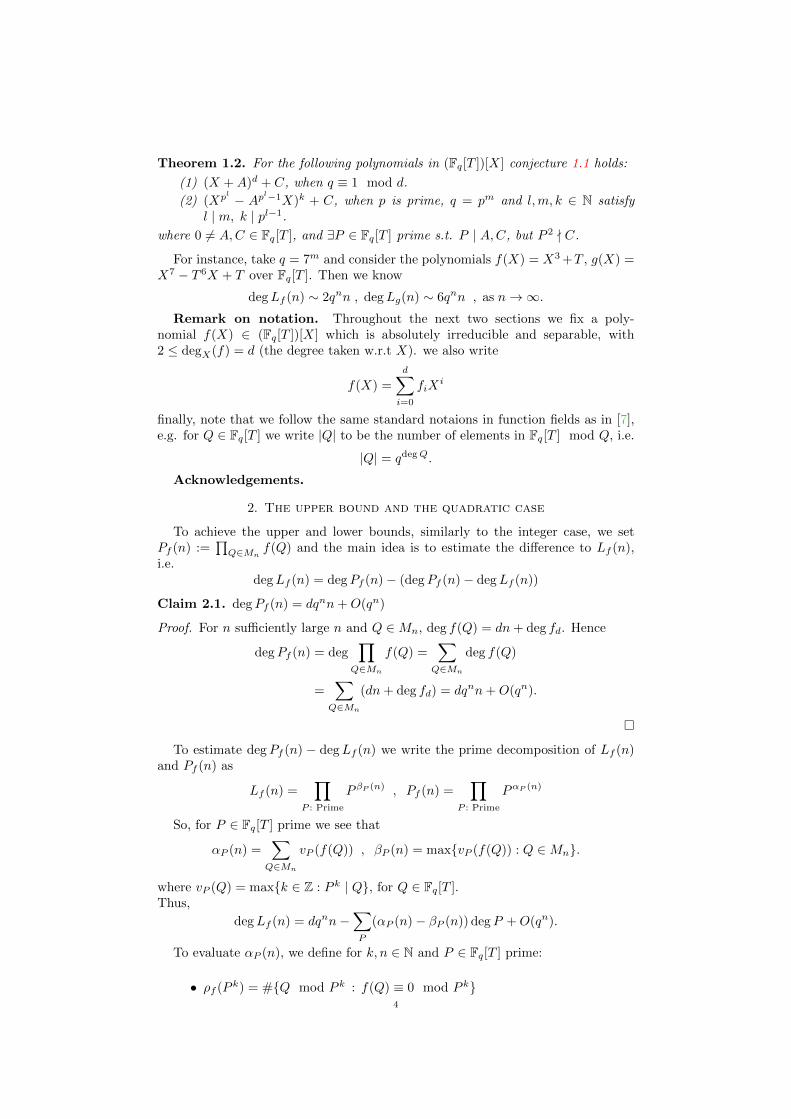
Theorem 1.2. For the following polynomials in (Fq[T ])[X] conjecture 1.1 holds:

(1) (X +A)d + C, when q ≡ 1 mod d.

(2) (Xpl − Apl−1X)k + C, when p is prime, q = pm and l,m, k ∈ N satisfyl | m, k | pl−1.

where 0 6= A,C ∈ Fq[T ], and ∃P ∈ Fq[T ] prime s.t. P | A,C, but P 2 - C.

For instance, take q = 7m and consider the polynomials f(X) = X3 +T , g(X) =X7 − T 6X + T over Fq[T ]. Then we know

degLf (n) ∼ 2qnn , degLg(n) ∼ 6qnn , as n→∞.Remark on notation. Throughout the next two sections we fix a poly-

nomial f(X) ∈ (Fq[T ])[X] which is absolutely irreducible and separable, with2 ≤ degX(f) = d (the degree taken w.r.t X). we also write

f(X) =

d∑i=0

fiXi

finally, note that we follow the same standard notaions in function fields as in [7],e.g. for Q ∈ Fq[T ] we write |Q| to be the number of elements in Fq[T ] mod Q, i.e.

|Q| = qdegQ.

Acknowledgements.

2. The upper bound and the quadratic case

To achieve the upper and lower bounds, similarly to the integer case, we setPf (n) :=

∏Q∈Mn

f(Q) and the main idea is to estimate the difference to Lf (n),i.e.

degLf (n) = degPf (n)− (degPf (n)− degLf (n))

Claim 2.1. degPf (n) = dqnn+O(qn)

Proof. For n sufficiently large n and Q ∈Mn, deg f(Q) = dn+ deg fd. Hence

degPf (n) = deg∏

Q∈Mn

f(Q) =∑Q∈Mn

deg f(Q)

=∑Q∈Mn

(dn+ deg fd) = dqnn+O(qn).

�

To estimate degPf (n) − degLf (n) we write the prime decomposition of Lf (n)and Pf (n) as

Lf (n) =∏

P : Prime

P βP (n) , Pf (n) =∏

P : Prime

PαP (n)

So, for P ∈ Fq[T ] prime we see that

αP (n) =∑Q∈Mn

vP (f(Q)) , βP (n) = max{vP (f(Q)) : Q ∈Mn}.

where vP (Q) = max{k ∈ Z : P k | Q}, for Q ∈ Fq[T ].Thus,

degLf (n) = dqnn−∑P

(αP (n)− βP (n)) degP +O(qn).

To evaluate αP (n), we define for k, n ∈ N and P ∈ Fq[T ] prime:

• ρf (P k) = #{Q mod P k : f(Q) ≡ 0 mod P k}4

• sf (P k, n) = #{Q ∈Mn : f(Q) ≡ 0 mod P k}Our main tool to estimate αP , βP is the following lemma:

Lemma 2.2. Let P ∈ Fq[T ] be prime.

(1) βP (n) = O(

dndegP

)(2) if P - disc(f) (a.k.a ”good” prime), then

αP (n) = qnρf (P )

|P | − 1+O

(n

degP

)and if P | disc(f) (a.k.a ”bad” prime), then

αP (n) = O(qn)

Proof. 1. Since P βP (n) | f(Q) for some Q ∈ Fq[T ], noting that f(Q) 6= 0 we get:

βP (n) degP ≤ deg f(Q)

and for sufficiently large n we have deg f(Q) = dn+ deg fd, thus

βP (n)� n

degP.

2. For any prime P we have

αP (n) =∑Q∈Mn

vP (f(Q)) =∑Q∈Mn

∑k≥0:

Pk|f(Q)

1

=∑

k� ndegP

∑Q∈Mn:

Pk|f(Q)

1 =∑

k� ndegP

sf (P k, n).

Noting that sf (P k, n) = ρf (P k)(⌊

#Mn

|Pk|

⌋+O(1)

)and ρf (P k)� 1, we get∑

k� ndegP

sf (P k, n) =∑

k� ndegP

ρf (P k)

(qn

|P |k +O(1)

)

=∑

k� ndegP

ρf (P k)

(qn

|P |k)

+O

(n

degP

).

Now, if P - disc(f), then by Hensel’s lemma we have ρf (P k) = ρf (P ), and so

αP (n) =∑

k� ndegP

ρf (P )

(qn

|P |k)

+O

(n

degP

)

= qnρf (P )∑

k� ndegP

(1

|P |

)k+O

(n

degP

)

= qnρf (P )

|P | − 1+O

(n

degP

)and if P | disc(f), then

αP (n) =∑

k� ndegP

ρf (P k)

(qn

|P |k)

+O

(n

degP

)

� qn∑

k� ndegP

(1

|P |

)k+O

(n

degP

)� qn.

�5

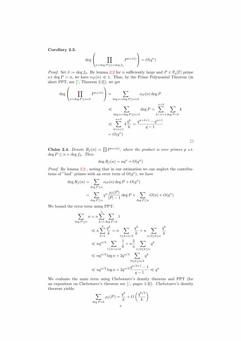
Corollary 2.3.

deg

∏n<degP≤n+deg fd

PαP (n)

= O(qn)

Proof. Set δ := deg fd. By lemma 2.2 for n sufficiently large and P ∈ Fq[T ] primes.t degP > n, we have αP (n) � 1. Thus, by the Prime Polynomial Theorem (inshort PPT, see [7, Theorem 2.2]), we get

deg

∏n<degP≤n+δ

PαP (n)

=∑

degn<degP≤n+δ

αP (n) degP

�∑

degn<degP≤n+δ

degP =

n+δ∑k=n+1

∑degP=k

k

�n+δ∑

k=n+1

kqk

k=qn+δ+1 − qn+1

q − 1

= O(qn)

�

Claim 2.4. Denote Rf (n) =∏PαP (n), where the product is over primes p s.t.

degP ≤ n+ deg fd. Then

degRf (n) = nqn +O(qn)

Proof. By lemma 2.2 , noting that in our estimation we can neglect the contribu-tions of ”bad” primes with an error term of O(qn), we have

degRf (n) =∑

degP≤n

αP (n) degP +O(qn)

=∑

degP≤n

qnρf (P )

|P | − 1degP +

∑degP≤n

O(n) +O(qn)

We bound the error term using PPT:∑degP≤n

n = n

n∑k=1

∑degP=k

1

� n

n∑k=1

qk

k= n

∑1≤k<n/2

qk

k+ n

∑n/2≤k≤n

qk

k

� nqn/2∑

1≤k<n/2

1

k+ n

2

n

∑n/2≤k≤n

qk

� nqn/2 log n+ 2qn/2∑

0≤k≤n/2

qk

� nqn/2 log n+ 2qn/2qn/2+1 − 1

q − 1� qn

We evaluate the main term using Chebotarev’s density theorem and PPT (foran exposition on Chebotarev’s theorem see [1, pages 1-2]). Chebotarev’s densitytheorem yields: ∑

degP=k

ρf (P ) =qk

k+O

(qk/2

k

)6

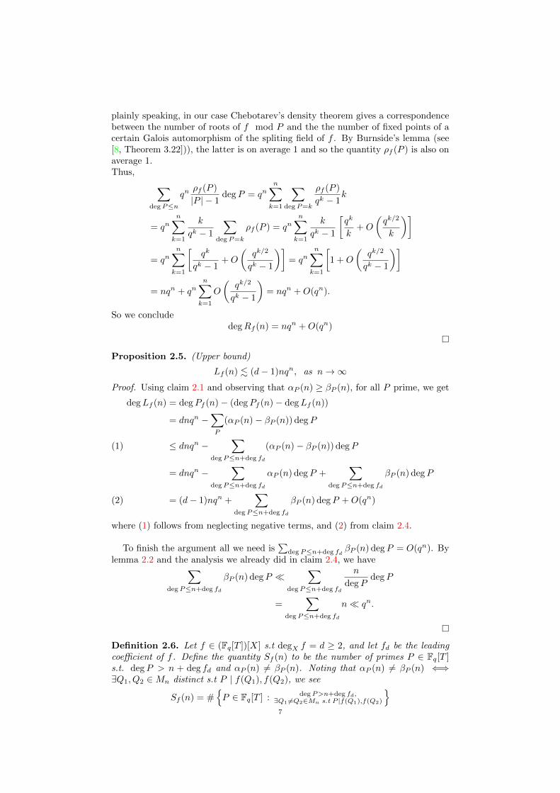
plainly speaking, in our case Chebotarev’s density theorem gives a correspondencebetween the number of roots of f mod P and the the number of fixed points of acertain Galois automorphism of the spliting field of f . By Burnside’s lemma (see[8, Theorem 3.22])), the latter is on average 1 and so the quantity ρf (P ) is also onaverage 1.Thus, ∑

degP≤n

qnρf (P )

|P | − 1degP = qn

n∑k=1

∑degP=k

ρf (P )

qk − 1k

= qnn∑k=1

k

qk − 1

∑degP=k

ρf (P ) = qnn∑k=1

k

qk − 1

[qk

k+O

(qk/2

k

)]

= qnn∑k=1

[qk

qk − 1+O

(qk/2

qk − 1

)]= qn

n∑k=1

[1 +O

(qk/2

qk − 1

)]

= nqn + qnn∑k=1

O

(qk/2

qk − 1

)= nqn +O(qn).

So we concludedegRf (n) = nqn +O(qn)

�

Proposition 2.5. (Upper bound)

Lf (n) . (d− 1)nqn, as n→∞Proof. Using claim 2.1 and observing that αP (n) ≥ βP (n), for all P prime, we get

degLf (n) = degPf (n)− (degPf (n)− degLf (n))

= dnqn −∑P

(αP (n)− βP (n)) degP

≤ dnqn −∑

degP≤n+deg fd

(αP (n)− βP (n)) degP(1)

= dnqn −∑

degP≤n+deg fd

αP (n) degP +∑

degP≤n+deg fd

βP (n) degP

= (d− 1)nqn +∑

degP≤n+deg fd

βP (n) degP +O(qn)(2)

where (1) follows from neglecting negative terms, and (2) from claim 2.4.

To finish the argument all we need is∑

degP≤n+deg fdβP (n) degP = O(qn). By

lemma 2.2 and the analysis we already did in claim 2.4, we have∑degP≤n+deg fd

βP (n) degP �∑

degP≤n+deg fd

n

degPdegP

=∑

degP≤n+deg fd

n� qn.

�

Definition 2.6. Let f ∈ (Fq[T ])[X] s.t degX f = d ≥ 2, and let fd be the leadingcoefficient of f . Define the quantity Sf (n) to be the number of primes P ∈ Fq[T ]s.t. degP > n + deg fd and αP (n) 6= βP (n). Noting that αP (n) 6= βP (n) ⇐⇒∃Q1, Q2 ∈Mn distinct s.t P | f(Q1), f(Q2), we see

Sf (n) = #{P ∈ Fq[T ] : degP>n+deg fd,

∃Q1 6=Q2∈Mn s.t P |f(Q1),f(Q2)

}7

Corollary 2.7. Let f ∈ (Fq[T ])[X] be absolutely irreducible and separable withdegX f = d ≥ 2. Then, conjecture 1.1 is equivalent to

Sf (n) = o(qn)

Moreover, we have

Sf (n)� qn

Proof. In the proof of the upper bound there is only one inequality (i.e. (1)),namely ∑

degP>n+deg fd

(αP (n)− βP (n)) degP > 0

so it suffices to prove that

Sf (n) = o(qn) ⇐⇒∑

degP>n+deg fd

(αP (n)− βP (n)) degP = o(nqn)

For P ∈ Fq[T ] prime, let 1P (n) =

{1 if αP (n) 6= βP (n)0 otherwise

.

Note that αP (n) 6= βP (n) ⇐⇒ ∃Q1, Q2 ∈ Mn distinct s.t P | f(Q1), f(Q2), andfor n sufficiently large degP > dn =⇒ αP (n) = 0. Hence, for n sufficiently largewe have

Sf (n) =∑

dn≥degP>n+deg fd

1P (n).

From lemma 2.2, for sufficiently large n, if degP > n then αP (n)� 1, so∑degP>n+deg fd

(αP (n)− βP (n)) degP �∑

dn≥degP>n+deg fd

1P (n) degP

�∑

dn≥degP>n+deg fd

1P (n)n

= Sf (n)n.

On the other hand∑degP>n+deg fd

(αP (n)− βP (n)) degP ≥∑

degP>n+deg fd

1P (n) degP

≥∑

degP>n+deg fd

1P (n)n

= Sf (n)n.

Therefore

Sf (n)n ≤∑

degP>n+deg fd

(αP (n)− βP (n)) degP � Sf (n)n

and so

Sf (n) = o(qn) ⇐⇒ degLf (n) ∼ (d− 1)qnn, as n→∞Finally, note that Sf (n)� qn follows from the upper bound. �

From this corollary we can easily achieve the quadratic case:

Corollary 2.8. Let f(X) = f2X2 + f1(T )X + f0(T ) be a quadratic polynomial

which is absolutely irreducible and separable over Fq[T ]. Then,

degLf (n) = nqn +O(qn), as n→∞8

Proof. for P prime in Fq[T ], and A,B ∈Mn we have

P | f(A), f(B) =⇒ P | f(A)− f(B) = (A−B)(f2A+ f2B + f1)

=⇒ P | (A−B) ∨ P | (f2A+ f2B + f1)

=⇒ degP ≤ max{n+ deg f2,deg f1}.Hence, for sufficiently large n if degP > n+ deg f2, then αP (n) = βP (n).Thus Sf (n)� 1, and by corollary 2.7 we are done. �

3. A lower bound

Remark. First we prove a lower bound similar to the one Maynard and Rudnickprovided (see [5, Theorem 1.2]), then will show an improved lower bound similar toAshwin Sah (see [10, Theorem 1.4]). Our arguments here are due to Sah, thoughin the improved lower bound something gets lost in translation to the function fieldcase (e.g. the characteristic is now positive), so we get a lower bound with somerestrictions.

Lemma 3.1. For n ≥ deg fd and P ∈ Fq[T ] prime such that degP ≥ n, we have

αP (n) ≤ d2

Proof. Note that ρf (P ) ≤ d, since f is irreducible over Fq[T ] of degree d. Andsince degP ≥ n, at most d polynomials Q ∈Mn satisfy P | f(Q). For such Q, andn ≥ deg fd, we get

degP d+1 ≥ nd+ n > nd+ deg fd = deg f(Q)

Hence,

αP (n) =∑Q∈Mn

vP (f(Q)) ≤∑

Q∈Mn:P |f(Q)

d ≤ d2

�

Proposition 3.2. (Lower bound) Let f ∈ Fq[T ] be absolutely irreducible andseparable. Then

Lf (n) &d− 1

d2nqn

Proof. By lemma 2.4 and claim 2.1, we get

(d− 1)nqn . degPf (n)

Rf (n)=

∑degP>n+deg fd

αP (n) degP

≤∑

degP>n+deg fd,αP (n)6=0

d2 degP ≤ d2 degLf (n)

from which the proposition follows. �

Lemma 3.3. For sufficiently large n, if char(Fq) > d, and P ∈ Fq[T ] is prime s.t.degP > n+ deg fd, then we have

αP (n) ≤ d(d− 1)

2.

Proof. Fix a prime P ∈ Fq[T ] s.t. degP > n+ deg fd.Denote Bi := #{Q ∈ Mn : P i | f(Q)}, for i ∈ N. By lemma 3.1, Bi = 0 ∀i > d,thus

αP (n) =∑Q∈Mn

∑i>0:

P i|f(Q)

1 =∑i>0

∑Q∈Mn:P i|f(Q)

1 =

d∑i=1

Bi

9

we claim Bi ≤ d− i for all 1 ≤ i ≤ d, from which the lemma follows immediately.Suppose for the sake of contradiction that Bi ≥ d − i + 1 for some 1 ≤ i ≤ d,

and let Q1, . . . , Qd−i+1 ∈ Mn be distinct s.t. P i | f(Qj) for all 1 ≤ j ≤ d − i + 1.Consider the value

A :=

d−i+1∑j=1

f(Qj)∏k 6=j(Qj −Qk)

.

This value (as we will see) is in Fq[T ]. To see this, note that from the theory ofLagrange interpolation polynomial, we have the identity: Let A1, . . . , An ∈ Fq[T ]be distinct for some n > 1. Then, for l ≥ n− 1

n∑j=1

Alj∏k 6=j(Aj −Ak)

=∑

a1+...+an=l−(n−1)

n∏j=1

Aajj

where the sum is over all tuples (a1, . . . , an) of nonnegative integers that sum tol − (n− 1). Note that for l < n− 1 this value vanishes.Thus we have

A =

d∑l=0

fl

d−i+1∑j=1

Qlj∏k 6=j(Qj −Qk)

=

d∑l=d−i

fl∑

a1+...+ad−i+1=l−(d−i)

d−i+1∏j=1

Qajj

where the inner sum is over all tuples (a1, . . . , ad−i+1) of nonnegative integers thatsum to l − (d− i).Therfore, A ∈ Fq[T ].

Note that the number of summands in the last inner sum (i.e. l = d) is(dd−i), and

from the condition that d > charFq, this value does not vanish in Fq . Thus, forsufficiently large n the degree of A is

degA = deg

fd ∑a1+...+ad−i+1=l−(d−i)

d−i+1∏j=1

Qajj

(1)= deg fd + max

a1+...+ad−i+1=l−(d−i)deg

d−i+1∏j=1

Qajj

= deg fd + i · n

where in (1) we used that Q1 . . . , Qd−i+1 are all monic of degree n.However, since P i | f(Qj) for all 1 ≤ j ≤ d− i+ 1, we have from the definition ofA that

P i | A∏

1≤j<k≤d−i+1

(Qj −Qk)

and since P i - (Qj −Qk) for any 1 ≤ j < k ≤ d− i+ 1, we see that P i | A. Whence

i · n+ deg fd < i · degP ≤ degA = i · n+ deg fd

which is a contradiction, so we obtain our result. �

Proposition 3.4. (Restricted lower bound) Let f ∈ Fq[T ] be absolutely irreducibleand separable s.t. 2 ≤ degX f < char(Fq). Then, we have

degLf (n) &2

dnqn

10

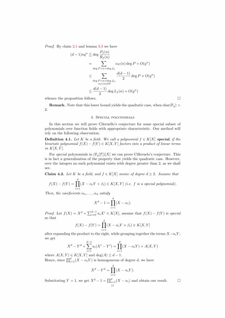
Proof. By claim 2.1 and lemma 3.3 we have

(d− 1)nqn . degPf (n)

Rf (n)

=∑

degP>n+deg fd

αP (n) degP +O(qn)

≤∑

degP>n+deg fd,αP (n)6=0

d(d− 1)

2degP +O(qn)

≤ d(d− 1)

2degLf (n) +O(qn)

whence the proposition follows. �

Remark. Note that this lower bound yields the quadratic case, when char(Fq) >2.

4. Special polynomials

In this section we will prove Cileruello’s conjecture for some special subset ofpolynomials over function fields with appropriate characteristic. Our method willrely on the following observation:

Definition 4.1. Let K be a field. We call a polynomial f ∈ K[X] special, if thebivariate polynomial f(X)− f(Y ) ∈ K[X,Y ] factors into a product of linear termsin K[X,Y ].

For special polynomials in (Fq[T ])[X] we can prove Cilleruelo’s conjecture. Thisis in fact a generalization of the property that yields the quadratic case. However,over the integers no such polynomial exists with degree greater than 2, as we shallsee.

Claim 4.2. Let K be a field, and f ∈ K[X] monic of degree d ≥ 2. Assume that

f(X)− f(Y ) =

d∏i=1

(X − αiY + βi) ∈ K[X,Y ] (i.e. f is a special polynomial).

Then, the coeeficients α1, . . . , αd satisfy

Xd − 1 =

d∏i=1

(X − αi).

Proof. Let f(X) = Xd +∑d−1i=0 aiX

i ∈ K[X], assume that f(X) − f(Y ) is specialso that

f(X)− f(Y ) =

d∏i=1

(X − αiY + βi) ∈ K[X,Y ]

after expanding the product to the right, while grouping together the termsX−αiY ,we get

Xd − Y d +

d−1∑i=1

ai(Xi − Y i) =

d∏i=1

(X − αiY ) +A(X,Y )

where A(X,Y ) ∈ K[X,Y ] and deg(A) ≤ d− 1.

Hence, since∏di=1(X − αiY ) is homogeneous of degree d, we have

Xd − Y d =

d∏i=1

(X − αiY ).

Substituting Y = 1, we get Xd − 1 =∏di=1(X − αi) and obtain our result. �11

Corollary 4.3. There are no special polynomials of degree greater than 2 withrational coefficients.

Proposition 4.4. Let f(X) ∈ (Fq[T ])[X] be monic and of degree d w.r.t. X. If fis special, absolutely irreducible and separable. Then

degLf (n) = (d− 1)nqn +O(qn).

Proof. Since f is special, by claim 4.2 we assume

f(X)− f(Y ) =

d∏i=1

(X − aiY + bi)

where bi ∈ Fq[T ] and ai ∈ F×q .Let P ∈ Fq[T ] prime, and Q1, Q2 ∈Mn distinct, so

P | f(Q1), f(Q2) =⇒ P | f(Q1)− f(Q2) =

d∏i=1

(Q1 + aiQ2 + bi)

=⇒ ∃i s.t. P | (Q1 + aiQ2 + bi)

=⇒ ∃i s.t. degP ≤ max{n , deg bi}.Hence, for sufficiently large n (i.e. n > maxi deg bi), if degP > n, then αP (n) =βP (n). Thus, Sf (n)� 1 and by corollary 2.7 we are done. �

So now our goal is to classify these special polynomials, and according to claim4.2 we will split our study to two cases, whether the degree divides the characteristicor not.

4.1. First case: gcd(d, p) = 1.

Example: Let f(X) = X3 + T ∈ (Fq[T ])[X], for some q ≡ 1 mod 3.Here we have a primitive third root of unity, namely ζ ∈ Fq, ζ3 = 1, and with thatin hand:

f(X)− f(Y ) = (X − Y )(X2 +XY + Y 2) = (X − Y )(X − ζY )(X − ζ2Y )

so f is special, absolutely irreducible and separable. Hence, by proposition 4.4 weget

degLf (n) = 2nqn +O(qn)

To generalize this example, note that for Xd − H to be irreducible is equivalentto requiring that if 4 - d, that for any prime divisor ` | d, we have H is not an`-th power in Fq(t), and in addition if 4 | d then H /∈ −4(Fq(t))4, see [6, Theorem14.1.4].

Claim 4.5. Let f(X) = Xd−H, where 2 ≤ d and H ∈ Fq[T ], monic with degH ≥1. Further assume that:

(1) ∀p | d prime, H /∈ (Fq[T ])p

(2) q ≡ 1 mod d

Then,

degLf (n) = (d− 1)nqn +O(qn)

Proof. By proposition 4.4, we need to verify that f is absolutely irreducible, sepa-rable and special. Firstly, separablity of f follows easily from q ≡ 1 mod d, and tosee that f is absolutely irreducible we’ll use the preceding theorem, noting that inthis case the second condition of the theorem is contained in the first one, since H

12

is monic. Let∏ki=1 P

nii = H be the prime decomposition of H, and denote by Fq

the algebraic closure of Fq. Take p | d prime, then the first assumption yields

H /∈ (Fq[T ])p ⇐⇒ p - gcd(n1, . . . , nk)

and since Fq is a perfect field, for each i all the roots of Pi are distinct, moreover∀i 6= j Pi and Pj have no roots in common, therefore

H /∈ (Fq[T ])p ⇐⇒ p - gcd(n1, . . . , nk)

whence, f is absolutely irreducible and separable.

Secondly, from the second assumption d | q − 1, and we know aq−1 = 1, ∀a ∈ F×q(| F×q |= q − 1). Hence, since F×q is a cyclic group, Fq contains all d-th roots ofunity, i.e. ∃a1, . . . , ad ∈ Fq s.t.

xd − 1 =

d∏i=1

(x− ai), in Fq[x](3)

substituting x = XY and multiplying by Y d in (3) we get

Xd − Y d =

d∏i=1

(X − aiY ), now in (Fq[T ])[X,Y ]

Whence, f is special and we obtain our result.�

Corollary 4.6. Let f(X) = (X + A)d − C ∈ (Fq[T ])[X], where q ≡ 1 mod d,0 6= A,C ∈ Fq[T ], and ∀p | d prime, C /∈ (Fq[T ])p and C is monic. Then we have

degLf (n) = (d− 1)qnn+O(qn), as n→∞

Proof. From the assumptions on C note that f(X − A) = Xd − C is absolutelyirreducible, hence so is f and separability follows immediately. To see that f isspecial, note that from q ≡ 1 mod d their exists ζ ∈ Fq a primitive d-th root ofunity, so

Xd − Y d =

d∏i=1

(X − ζiY )

and after shifting (X,Y ) 7→ (X +A, Y +A), we get

f(X)− f(Y ) = (X +A)d − (Y +A)d

=

d∏i=1

(X +A− ζi(Y +A))

=

d∏i=1

[X − ζiY + (1− ζi)A].

Thus f is special, and by proposition 4.4 we obtain our result. �

Proposition 4.7. Let f(X) = Xd +Ad−1Xd−1 + . . .+A1X +A0 ∈ (Fq[T ])[X] be

a special polynomial, of degree d ≥ 3 where gcd(q, d) = 1. Then ∃A,C ∈ Fq[T ] s.t.

f(X) = (X +A)d + C.

Proof. Assume WLOG that Ad−1 = 0, otherwise consider f(X) = f(X − 1dAd−1)

which is also special (we assume that gcd(d, p) = 1 so that d is invertible in Fq)13

and its (d− 1)-coefficient is zero.So, since f is special, we write

f(X)− f(Y ) = (X − Y )

d−1∏i=1

(X − ζidY + bi)

where ζd ∈ Fq is a primitive d-th root of unity (this is a necessary condition byclaim 4.2), and bi ∈ Fq[T ]∀i.Hence, we have

f(X)− f(Y )

X − Y =

d−1∏i=1

(X − ζidY + bi)(4)

on the left hand side the degree (d− 2)-homogeneous part vanishes, i.e.

Ad−1Xd−1 − Y d−1

X − Y = 0.

Hence comparing the (d− 2)-homogeneous part of both sides in (4) yields

0 =

d−1∑i=1

bi

d−1∏j=1j 6=i

(X − ζjdY )

Take any 1 ≤ i0 ≤ d− 1, and substitute X = ζi0d , Y = 1 to get

0 = bi0∏j=1j 6=i0

(ζi0d − ζjd)

since all the terms in the sum vanish except the i0- term.Thus bi = 0 for any 1 ≤ i ≤ d− 1, and therefore

f(X)− f(Y ) = (X − Y )

d−1∏i=1

(X − ζidY ) = Xd − Y d

so f(X) = Xd +A0, and we obtain our result. �

Thus, we have classified all special polynomials, with degree co-prime to thecharacteristic of Fq.

4.2. Second case: gcd(d, p) = p.

Example: Take q = 3m and consider f(X) = X3 + 2X + T ∈ (F3m [T ])[X].Note that for any Q ∈Mn

f(Q) = Q3 + 2Q+ T = 0 ⇐⇒ Q(Q2 + 2) = −Tbut the degree of the left hand side is divisible by three, so this cannot happen.Thus, f is absolutely irreducible and separable. Moreover

f(X)− f(Y ) = X3 − Y 3 + 2(X − Y )

= (X − Y )(X2 +XY + Y 2 + 2)

= (X − Y )(X − Y + 1)(X − Y + 2)

Therefore, f is also special. So, in this case conjecture 1.1 holds .

Proposition 4.8. Let f ∈ (Fq[T ])[X] be of degree pl (w.r.t. X), where q = pm

and m, l ≥ 1. Then, f is a special polynomial if and only if the following conditionshold:

14

(1) f is of the form

f(X) = Xpl +

l−1∑k=0

ApkXpk +A0

meaning all the d-th coefficients of f vanish when d 6= 0 and d is not apower of p.

(2) f(X)− f(0) factors into a product of linear terms in (Fq[T ])[X].

Proof. Let f(X) = Xpl +∑pl−1k=0 AkX

k. Assume that f is special, then by claim

4.2 (noting that by the Frobenius endomorphism Xpl − 1 = (X − 1)pl

) we have

f(X)− f(Y ) =

pl∏k=1

(X − Y +Bk) ∀k Bk ∈ Fq[T ]

Take 0 < d < pl, then by comparing the d-th homogeneous part in both sides ofthe above we get

Ad(Xd − Y d) =

∑1≤k1<...<kpl−d

≤pl(X − Y )d

pl−d∏i=1

Bki

= (X − Y )d∑

1≤k1<...<kpl−d≤pl

pl−d∏i=1

Bki .

Thus, since Xd − Y d = (X − Y )d if and only if d is a p-th power, we conclude thatfor d > 0 which is not a power of p we get

Ad =∑

1≤k1<...<kpl−d≤pl

pl−d∏i=1

Bki = 0

which is condition 1. So now

f(X) = Xpl +

l−1∑k=0

ApkXpk +A0.

Hence, by the Frobenius endomorphism and the assumption that f is special, wehave

f(X)− f(Y ) = (X − Y )pl

+

l−1∑k=0

Apk(X − Y )pk

+A0

=

pl∏k=1

(X − Y +Bk).

Substitute X − Y = Z to obtain

f(Z)− f(0) = Zpl

+

l−1∑k=0

ApkZpk =

pl∏k=1

(Z +Bk)

which is condition 1.Now, for the other direction assume that both conditions hold for f . Then we have

f(Z)− f(0) = Zpl

+

l−1∑k=0

ApkZpk =

pl∏k=1

(Z +Bk)

where ∀k, BK ∈ Fq[T ]. hence by substituting Z = X − Y and using the Frobeniusendomorphism, we get our result. �

15

Remark. This proposition reduces the classification of special polynomials ofdegree pl in Fq to the classification of polynomials of degree pl−1 that factor into aproduct of linear terms. For small degrees we can get conditions on the coefficientsdue to Vieta’s equations, as the next claim suggests.

Claim 4.9. Take q = 3m for some 0 < m ∈ Z. Let f ∈ (Fq[t])[X] with degX f = 9.Then f is special if and only if

f(X) = X9 + (C21 + C2

2 )(C41 + C4

2 )X3 + C21C

22 (C2

1 − C22 )2X + C

for any C1, C2, C ∈ Fq[T ].

Proof. By proposition 4.8, f is special if and only if f is of the form

f(X) = X9 +AX3 +BX + C

and ∃Bk ∈ Fq[T ], k = 1, . . . 8 s.t.

X9 +AX3 +BX = X[(X2)4 +AX2 +B] = X

8∏k=1

(X −Bk)

Since all monomials (in the brackets) are of even degree this is true if and only if

Y 4 +AY +B =

4∏k=1

(Y −Ak)

where A1, A2, A3, A4 ∈ Fq[T ] are squares.So, by Vieta’s equations we need to solve the following:

(1)∑

1≤i≤4Ai = 0

(2)∑

1≤i<j≤4AiAj = 0.

Squaring the first equation and subtracting twice the second one we get

(1) A4 = −(A1 +A2 +A3)(2)

∑1≤i≤4

A2i = 0.

Inserting equation (1) into (2) we get a quadratic equation in A3 with parametersA1, A2

0 = A21 +A2

2 +A23 + (A1 +A2 +A3)2

⇐⇒ 0 = 2A3 + 2(A1 +A2)A3 +A21 +A2

2 + (A1 +A2)2

⇐⇒ 0 = 2A3 + 2(A1 +A2)A3 + 2A21 + 2A2

2 + 2A1A2.

Noting that 2 ≡ −1 since the characteristic is 3, the solution is:

A3 =A1 +A2 ±

√(A1 +A2)2 − 2(2A2

1 + 2A22 + 2A1A2)

4

= A1 +A2 ±√A2

1 + 2A1A2 +A22 −A2

1 −A22 −A1A2

= A1 +A2 ±√A1A2 =

(√A1 ±

√A2

)2.

If A3 =(√A1 +

√A2

)2, then by the first equation we get:

A4 = −A1 −A2 −A1 −A2 −√A1A2 = A1 +A2 −

√A1A2

=(√

A1 −√A2

)216

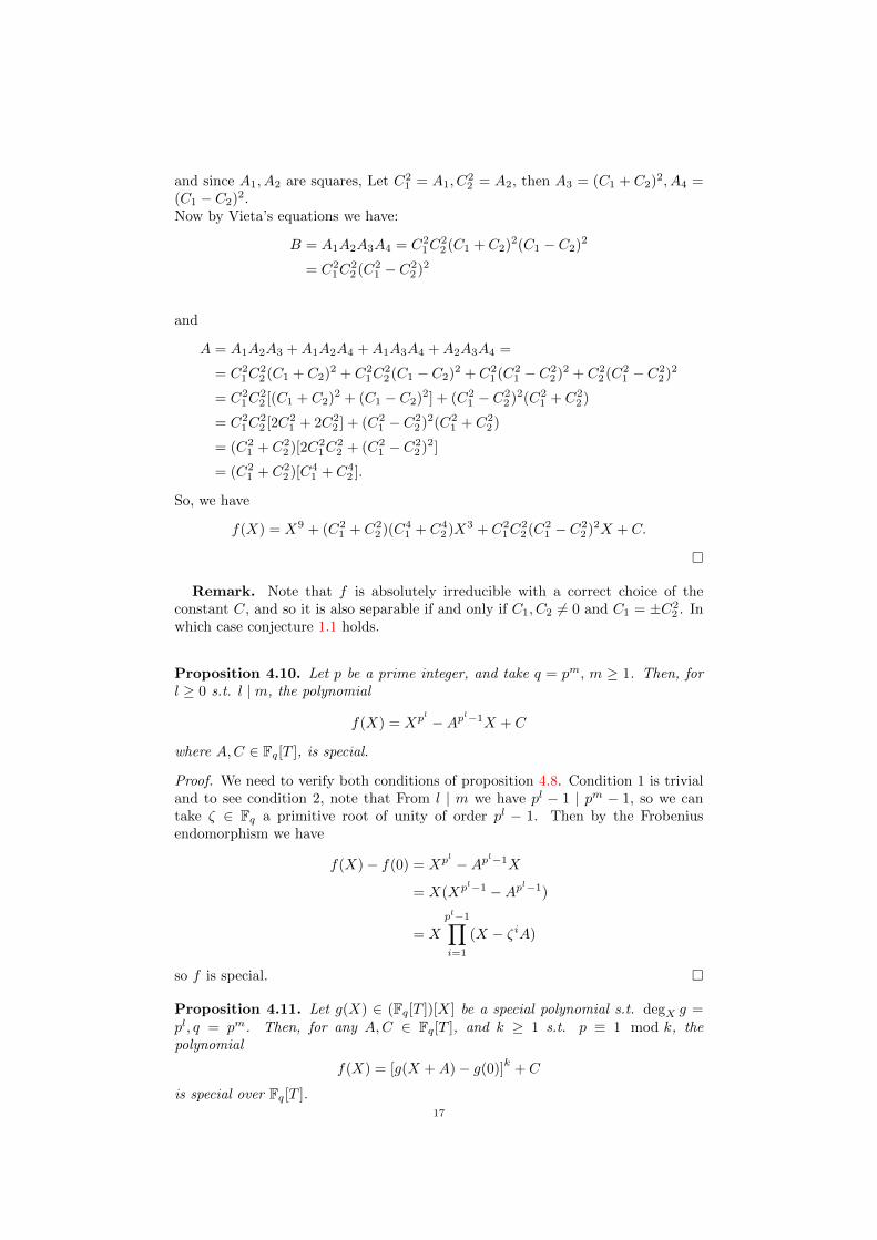
and since A1, A2 are squares, Let C21 = A1, C

22 = A2, then A3 = (C1 + C2)2, A4 =

(C1 − C2)2.Now by Vieta’s equations we have:

B = A1A2A3A4 = C21C

22 (C1 + C2)2(C1 − C2)2

= C21C

22 (C2

1 − C22 )2

and

A = A1A2A3 +A1A2A4 +A1A3A4 +A2A3A4 =

= C21C

22 (C1 + C2)2 + C2

1C22 (C1 − C2)2 + C2

1 (C21 − C2

2 )2 + C22 (C2

1 − C22 )2

= C21C

22 [(C1 + C2)2 + (C1 − C2)2] + (C2

1 − C22 )2(C2

1 + C22 )

= C21C

22 [2C2

1 + 2C22 ] + (C2

1 − C22 )2(C2

1 + C22 )

= (C21 + C2

2 )[2C21C

22 + (C2

1 − C22 )2]

= (C21 + C2

2 )[C41 + C4

2 ].

So, we have

f(X) = X9 + (C21 + C2

2 )(C41 + C4

2 )X3 + C21C

22 (C2

1 − C22 )2X + C.

�

Remark. Note that f is absolutely irreducible with a correct choice of theconstant C, and so it is also separable if and only if C1, C2 6= 0 and C1 = ±C2

2 . Inwhich case conjecture 1.1 holds.

Proposition 4.10. Let p be a prime integer, and take q = pm, m ≥ 1. Then, forl ≥ 0 s.t. l | m, the polynomial

f(X) = Xpl −Apl−1X + C

where A,C ∈ Fq[T ], is special.

Proof. We need to verify both conditions of proposition 4.8. Condition 1 is trivialand to see condition 2, note that From l | m we have pl − 1 | pm − 1, so we cantake ζ ∈ Fq a primitive root of unity of order pl − 1. Then by the Frobeniusendomorphism we have

f(X)− f(0) = Xpl −Apl−1X= X(Xpl−1 −Apl−1)

= X

pl−1∏i=1

(X − ζiA)

so f is special. �

Proposition 4.11. Let g(X) ∈ (Fq[T ])[X] be a special polynomial s.t. degX g =pl, q = pm. Then, for any A,C ∈ Fq[T ], and k ≥ 1 s.t. p ≡ 1 mod k, thepolynomial

f(X) = [g(X +A)− g(0)]k

+ C

is special over Fq[T ].17

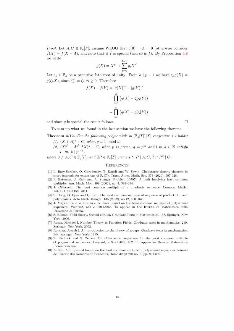
Proof. Let A,C ∈ Fq[T ], assume WLOG that g(0) = A = 0 (otherwise consider

f(X) = f(X − A), and note that if f is special then so is f). By Proposition 4.8we write

g(X) = Xpl +

l−1∑i=0

giXpi

Let ζk ∈ Fq be a primitive k-th root of unity. From k | p − 1 we have ζkg(X) =

g(ζkX), since ζpi

k = ζk ∀i ≥ 0. Therefore

f(X)− f(Y ) = [g(X)]k − [g(Y )]

k

=

k∏i=1

(g(X)− ζikg(Y )

)=

k∏i=1

(g(X)− g(ζikY )

)and since g is special the result follows. �

To sum up what we found in the last section we have the following thorem:

Theorem 4.12. For the following polynomials in (Fq[T ])[X] conjecture 1.1 holds:

(1) (X +A)d + C, when q ≡ 1 mod d.

(2) (Xpl − Apl−1X)k + C, when p is prime, q = pm and l,m, k ∈ N satisfyl | m, k | pl−1.

where 0 6= A,C ∈ Fq[T ], and ∃P ∈ Fq[T ] prime s.t. P | A,C, but P 2 - C.

References

[1] L. Bary-Soroker, O. Gorodetsky, T. Karidi and W. Sawin. Chebotarev density theorem in

short intervals for extensions of Fq(T ). Trans. Amer. Math. Soc. 373 (2020), 597-628.[2] P. Bateman, J. Kalb and A. Stenger. Problem 10797: A limit involving least common

multiples. Am. Math. Mon. 109 (2002), no. 4, 393–394.

[3] J. Cilleruelo. The least common multiple of a quadratic sequence. Compos. Math.,147(4):1129–1150, 2011.

[4] S. Hong, G. Qian and Q. Tan, The least common multiple of sequence of product of linear

polynomials. Acta Math. Hungar. 135 (2012), no.12, 160–167.[5] J. Maynard and Z. Rudnick. A lower bound on the least common multiple of polynomial

sequences. Preprint, arXiv:1910.13218. To appear in the Rivista di Matematica dellaUniversita di Parma.

[6] S. Roman. Field theory. Second edition. Graduate Texts in Mathematics, 158. Springer, New

York, 2006.[7] Rosen, Michael I. Number Theory in Function Fields. Graduate texts in mathematics, 210.

Springer, New York, 2002.

[8] Rotman, Joseph j. An introduction to the theory of groups. Graduate texts in mathematics,148. Springer, New York, 1995.

[9] Z. Rudnick and S. Zehavi. On Cilleruelo’s conjecture for the least common multiple

of polynomial sequences. Preprint, arXiv:1902.01102. To appear in Revista MatematicaIberoamericana.

[10] A. Sah. An improved bound on the least common multiple of polynomial sequences. Journal

de Theorie des Nombres de Bordeaux, Tome 32 (2020) no. 3, pp. 891-899.

18

אבסטרקט

ממש גדולה שמעלתו כך שלמים, מקדמים עם f פריק אי פולינום שלכל שיער סילרואלומקיימת הראשונים המספרים Nב־ f של הערכים של ביותר הקטנה המשותפת הכפולה מאחד,הוכיח הוא לאינסוף. שואף N כאשר ,log lcm(f(1), . . . , f(N)) ∼ (deg f − 1)N logNחוקרים אנו יותר. גבוהה במעלה דוגמה אף ידועה לא .deg f = 2 המקרה עבור רק זאתבחוג השלמים המספרים את מחליפים כאשר פונקציות, שדות מעל זו השערה של האנלוגיה אתההשערה של מקרים למצוא מסוגלים אנו הללו ההגדרות תחת סופי. שדה מעל הפולינומיםשהפולינום התכונה שלהם , f(X) ”מיוחדים” פולינומים כולן הללו הדוגמאות גבוהות. במעלות

הבסיס. בשדה לינארים לגורמים מתפרק f(X) − f(Y ) המשתנים מרובה

פונקציות שדות מעל ביותר הקטנה המשותפת הכפולה בעיית

התואר לקבלת מהדרישות כחלק הוגש זה חיבוראביב, תל באוניברסיטת (M.Sc.) אוניברסיטה״ ״מוסמך

המתמטיקה למדעי הספר בית

ידי עללאומי איתי

של בהדרכתו הוכנה העובדהרודניק זאב פרופסור

תשפ״א ניסן,

the lcm problem for function fields

Documents