1/

acNeilled to have

ueMacNeillere est assuré

tisticall concept,both setsordered

C. R. Acad. Sci. Paris, Ser. I 341 (2005) 583–586http://france.elsevier.com/direct/CRASS

Probability Theory

The lattice-theoretic structure of setsof bivariate copulas and quasi-copulas

Roger B. Nelsena, Manuel Úbeda Floresb

a Department of Mathematical Sciences, Lewis& Clark College, 0615 S.W. Palatine Hill Road, Portland, OR 97219, USAb Departamento de Estadística y Matemática Aplicada, Universidad de Almería, Carretera de Sacramento s/n,

La Cañada de San Urbano, 04120 Almería, Spain

Received 20 July 2005; accepted after revision 15 September 2005

Available online 11 October 2005

Presented by Paul Deheuvels

Abstract

In this Note we show that the set of quasi-copulas is a complete lattice, which is order-isomorphic to the Dedekind–Mcompletion of the set of copulas. Consequently, any set of copulas sharing a particular statistical property is guaranteepointwise best-possible bounds within the set of quasi-copulas.To cite this article: R.B. Nelsen, M. Úbeda Flores, C. R. Acad.Sci. Paris, Ser. I 341 (2005). 2005 Académie des sciences. Published by Elsevier SAS. All rights reserved.

Résumé

La structure réseau-théorique des ensembles de copules et quasi-copules bivariées. Dans cette Note, nous montrons ql’ensemble des quasi-copules est un treillis complet, qui est isomorphe au sens de l’ordre à la complétion de Dedekind–de l’ensemble des copules. En conséquence, tout ensemble de copules qui possède une propriété statistique particuliède réaliser les meilleures bornes ponctuelles parmi l’ensemble des quasi-copules.Pour citer cet article : R.B. Nelsen, M. ÚbedaFlores, C. R. Acad. Sci. Paris, Ser. I 341 (2005). 2005 Académie des sciences. Published by Elsevier SAS. All rights reserved.

1. Introduction

Copulas – bivariate distribution functions with uniform margins – have proven to be remarkably useful in stamodelling and in the study of dependence and association of random variables. Quasi-copulas, a more generashare many properties with copulas. The set of copulas is a proper subset of the set of quasi-copulas, andhave a natural partial ordering. The purpose of this Note is to investigate some properties of those partiallysets (posets).

A copulais a functionC : [0,1]2 → [0,1] which satisfies (C1) the boundary conditionsC(t,0) = C(0, t) = 0 andC(t,1) = C(1, t) = t for all t ∈ [0,1], and (C2) the 2-increasing property, i.e.,VC([u1, u2] × [v1, v2]) = C(u2, v2) −

E-mail addresses:nelsen@lclark.edu (R.B. Nelsen), mubeda@ual.es (M. Úbeda Flores).

1631-073X/$ – see front matter 2005 Académie des sciences. Published by Elsevier SAS. All rights reserved.doi:10.1016/j.crma.2005.09.026

584 R.B. Nelsen, M. Úbeda Flores / C. R. Acad. Sci. Paris, Ser. I 341 (2005) 583–586

s

any

distrib-obabilityhe

xistoer

),

ne

C(u2, v1) − C(u1, v2) + C(u1, v1) � 0 for all u1, u2, v1, v2 in [0,1] such thatu1 � u2 andv1 � v2. The importanceof copulas in statistics stems in part from Sklar’s theorem [6]: LetH be a bivariate distribution function with marginF andG. Then there exists a copulaC (which is uniquely determined on RangeF × RangeG) such thatH(x,y) =C(F(x),G(y)) for all x, y in [−∞,∞]. Thus copulas link joint distribution functions to their margins. ForcopulaC we haveW(u,v) = max(0, u + v − 1) � C(u, v) � min(u, v) = M(u,v) for all (u, v) in [0,1]2. M andW are copulas, and the order relation in the above inequality leads to a partial order≺ (also known asconcordanceorder) on the setC of copulas:C1 ≺ C2 if and only if C1(u, v) � C2(u, v) for all (u, v) in [0,1]2. See [4] for moredetails.

The concept of a quasi-copula was introduced by Alsina et al. [1] in order to characterize operations onution functions that can or cannot be derived from operations on random variables defined on the same prspace. Aquasi-copulais a functionQ : [0,1]2 → [0,1] which satisfies condition (C1), but in place of (C2), tweaker conditions (i)Q is non-decreasing in each variable, and (ii) the Lipschitz condition|Q(u1, v1)−Q(u2, v2)| �|u1 − u2| + |v1 − v2| for all (u1, v1), (u2, v2) in [0,1]2 (see [3]). While every copula is a quasi-copula, there eproper quasi-copulas, i.e., quasi-copulas which are not copulas. As with copulas, the setQ of quasi-copulas is alspartially ordered by≺, and for any quasi-copulaQ we haveW ≺ Q ≺ M . Finally, Q \ C denotes the set of propquasi-copulas.

We will also need some notions from lattice theory. Given two elementsx andy of a poset(P,≺), let x ∨ y

denote thejoin of x andy (when it exists); similarly for∨

S, whereS is a subset ofP ; x ∧ y denotes themeetofx andy (when it exists); and similarly for

∧S. In particular, for any pairQ1 andQ2 of quasi-copulas (or copulas

Q1 ∨ Q2 = inf{Q ∈ Q | Q1 ≺ Q, Q2 ≺ Q} andQ1 ∧ Q2 = sup{Q ∈ Q | Q ≺ Q1, Q ≺ Q2}. If the join or meetis found within a particular posetP , we subscript

∨P S. Given two posetsA andB, we say thatA is join-dense

(respectively,meet-dense) in B if for any D in B, there exists a setS ⊆ A such thatD = ∨S (respectively,D = ∧

S).If x ∈ P , then↓x = {s ∈ P | s ≺ x} and↑x = {s ∈ P | s x}. A posetP �= ∅ is a lattice if for every x, y in P , x ∨ y

andx ∧ y are inP ; andP is acomplete latticeif for everyS ⊆ P ,∨

S and∧

S are inP .

2. The lattice of quasi-copulas

We begin with some basic results on the structure of the posetsQ, C andQ \ C.

Theorem 2.1. Q is a complete lattice; however, neitherC nor Q \ C is a lattice.

Proof. Let S be any set of quasi-copulas, and defineQS(u, v) = sup{Q(u,v) | Q ∈ S} andQS(u, v) = inf{Q(u,v) |

Q ∈ S} for each(u, v) in [0,1]2. SinceQS andQS

are quasi-copulas [5, Theorem 2.2], it now follows that∨

S

(= QS) and∧

S (= QS) are inQ, henceQ is a complete lattice.

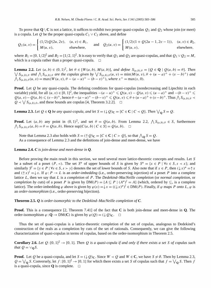
Now suppose thatC is a lattice, and consider the following copulas:C1(u, v) = min(u, v,max(0, u − 2/3, v −1/3, u + v − 1)), C2(u, v) = C1(v,u), C3(u, v) = min(u, v,max(0, u − 1/3, v − 1/3, u + v − 2/3)) andC4(u, v) =min(u, v,max(1/3, u − 1/3, v − 1/3, u + v − 1)). The copulasC1, . . . ,C4 are singular, and the support of each oconsists of two or three line segments in[0,1]2 with slope+1, as shown in Fig. 1. IfC is a lattice,C = C1 ∨ C2

exists and is a copula. HenceC(1/3,2/3) � C1(1/3,2/3) = 1/3 = M(1/3,2/3), so thatC(1/3,2/3) = 1/3. Simi-larly (usingC2), C(2/3,1/3) = 1/3. SinceC1 ≺ C3 andC2 ≺ C3, C ≺ C3 and soC(1/3,1/3) � C3(1/3,1/3) = 0,thusC(1/3,1/3) = 0. Similarly C(2/3,2/3) � C4(2/3,2/3) = 1/3 = W(2/3,2/3), so C(2/3,2/3) = 1/3. HenceVC([1/3,2/3]2) = −1/3, i.e.,C is a proper quasi-copula; a contradiction.

Fig. 1. The supports ofC1, C2, C3, andC4 (left to right).

R.B. Nelsen, M. Úbeda Flores / C. R. Acad. Sci. Paris, Ser. I 341 (2005) 583–586 585

)

in each

ts. Let

dekind’sllowing

,

To prove thatQ \ C is not a lattice, it suffices to exhibit two proper quasi-copulasQ1 andQ2 whose join (or meetis a copula. LetQ be the proper quasi-copulaC1 ∨ C2 above, and define

Q1(u, v) ={

(1/2)Q(2u,2v), (u, v) ∈ B1,

M(u, v), elsewhere,and Q2(u, v) =

{(1/2)(1+ Q(2u − 1,2v − 1)), (u, v) ∈ B2,

M(u, v), elsewhere,

whereB1 = [0,1/2]2 andB2 = [1/2,1]2. It is easy to verify thatQ1 andQ2 are quasi-copulas, and thatQ1∨Q2 = M ,which is a copula rather than a proper quasi-copula.�Lemma 2.2. Let (a, b) ∈ (0,1)2, let θ ∈ [W(a,b),M(a, b)], and defineS(a,b),θ = {Q ∈ Q | Q(a,b) = θ}. Then∨

S(a,b),θ and∧

S(a,b),θ are the copulas given by∨

S(a,b),θ (u, v) = min(M(u, v), θ + (u − a)+ + (v − b)+) and∧S(a,b),θ (u, v) = max(W(u, v), θ − (a − u)+ − (b − v)+), wherex+ = max(x,0).

Proof. Let Q be any quasi-copula. The defining conditions for quasi-copulas (nondecreasing and Lipschitzvariable) yield, for all(u, v) ∈ [0,1]2, the inequalities−(a − u)+ � Q(u,v) − Q(a,v) � (u − a)+ and−(b − v)+ �Q(a,v)−Q(a,b) � (v−b)+, henceθ −(a−u)+ −(b−v)+ � Q(u,v) � θ +(u−a)+ +(v−b)+. Thus

∧S(a,b),θ ≺

Q ≺ ∨S(a,b),θ , and these bounds are copulas [4, Theorem 3.2.2].�

Lemma 2.3. LetQ ∈ Q be any quasi-copula, and letS = (↓Q)C = {C ∈ C | C ≺ Q}. Then∨

Q S = Q.

Proof. Let (a, b) any point in (0,1)2, and setθ = Q(a,b). From Lemma 2.2,∧

S(a,b),θ ∈ S, furthermore∧S(a,b),θ (a, b) = θ = Q(a,b). Hence sup{C(a, b) | C ∈ S} = Q(a,b). �Note that Lemma 2.3 also holds withS = (↑Q)C = {C ∈ C | C Q}, so that

∧Q S = Q.

As a consequence of Lemma 2.3 and the definitions of join-dense and meet-dense, we have

Lemma 2.4. C is join-dense and meet-dense inQ.

Before proving the main result in this section, we need several more lattice-theoretic concepts and resulS

be a subset of a poset(P,≺). The setSu of upper bounds ofS is given bySu = {x ∈ P | ∀s ∈ S, s ≺ x}; andsimilarly Sl = {y ∈ P | ∀s ∈ S, s y} denotes the set of lower bounds ofS. Also note that ifx ∈ P , then(↓x)u =↑x

and(↑x)l =↓x. If ϕ :P → L is anorder-imbedding(i.e., order-preserving injection) of a posetP into a completelatticeL, then we say thatL is acompletionof P . TheDedekind–MacNeille completion(or normal completion, orcompletion by cuts) of a posetP is given by DM(P ) = {A ⊆ P | (Au)l = A} (which, ordered by⊆, is a completelattice). The order-imbeddingϕ above is given byϕ(x) =↓x = ((↓x)u)l ∈ DM(P ). Finally, if ϕ mapsP ontoL, ϕ isanorder-isomorphism(i.e., order-preserving bijection).

Theorem 2.5. Q is order-isomorphic to the Dedekind–MacNeille completion ofC.

Proof. This is a consequence [2, Theorem 7.41] of the fact thatC is both join-dense and meet-dense inQ. Theorder-isomorphismϕ : Q → DM(C) is given byϕ(Q) = (↓Q)C. �

Thus the set of quasi-copulas is a lattice-theoretic completion of the set of copulas, analogous to Deconstruction of the reals as a completion by cuts of the set of rationals. Consequently, we can give the focharacterization of quasi-copulas in terms of copulas, based on the order-isomorphism in Theorem 2.5.

Corollary 2.6. Let Q : [0,1]2 → [0,1]. ThenQ is a quasi-copula if and only if there exists a setS of copulas suchthatQ = ∨QS.

Proof. Let Q be a quasi-copula, and letS = (↓Q)C. SinceW ≺ Q andW ∈ C, we haveS �= ∅. Then by Lemma 2.3Q = ∨

Q S. Conversely, letf : [0,1]2 → [0,1] for which there exists a setS of copulas such thatf = ∨Q S. Thenf

is a quasi-copula, sinceQ is complete. �

586 R.B. Nelsen, M. Úbeda Flores / C. R. Acad. Sci. Paris, Ser. I 341 (2005) 583–586

pulas.las. The

t

leu-

ons. Theh project

b. Lett. 1

999) 193–

functions,

Corollary 2.6 also holds with joins replaced by meets.In the proof of Theorem 2.1 we used quasi-copulas which were the join of a finite number (two) of co

However, there exist quasi-copulas which cannot be written as the meet or join of any finite set of copufollowing result proves the result for meets (joins are similar).

Proposition 2.7. Let Q be a quasi-copula for whichQ(u,v) = max(u − 1/3, v − 1/3), (u, v) ∈ [1/3,2/3]2, and letC0 denote any set of copulas such thatQ = ∧

C0. ThenC0 has infinitely many members.

Proof. We first note that there exist quasi-copulasQ with the propertyQ(u,v) = max(u − 1/3, v − 1/3) for(u, v) ∈ [1/3,2/3]2 [5, Example 2.1]. LetC0 be any set of copulas such thatQ = ∧

C0, and letC be a (fixed) elemenof C0. SinceQ(1/3,2/3) = 1/3= M(1/3,2/3), it follows thatC(1/3,2/3) = 1/3; and similarlyC(2/3,1/3) = 1/3.Thus for someε, δ in [0,1/3] with ε + δ � 1/3, C(1/3,1/3) = ε andC(2/3,2/3) = 1/3 + δ. Now let (u, v) bea (fixed) point in[1/3,2/3]2. ThenVC([u,1] × [v,2/3]) � 0 impliesC(u, v) � C(u,2/3) + v − 2/3 � v − 1/3,and similarlyC(u, v) � u − 1/3. Furthermore,VC([u,1] × [v,1]) � δ impliesC(u, v) � u + v − 1 + δ, and henceC(u, v) � max(ε, u − 1/3, v − 1/3, u + v − 1 + δ) for any (u, v) in [1/3,2/3]2. But max(ε, u − 1/3, v − 1/3,

u + v − 1 + δ) = v − 1/3 only on the rectangle[1/3,2/3 − δ] × [1/3 + ε,2/3], a proper subset of the triang{(u, v) | 1/3 � u � v � 2/3} whereQ(u,v) = v − 1/3, and henceQ cannot be the meet of a finite number of coplas. �Acknowledgements

The authors acknowledge the support of the Junta de Andalucía (Spain), and their respective institutisecond author also thanks the support by the Ministerio de Ciencia y Tecnología (Spain) under researcBFM2003-06522.

References

[1] C. Alsina, R.B. Nelsen, B. Schweizer, On the characterization of a class of binary operations on distribution functions, Statist. Proba7(1993) 85–89.

[2] B.A. Davey, H.A. Priestley, Introduction to Lattices and Order, second ed., Cambridge University Press, Cambridge, 2002.[3] C. Genest, J.J. Quesada Molina, J.A. Rodríguez Lallena, C. Sempi, A characterization of quasi-copulas, J. Multivariate Anal. 69 (1

205.[4] R.B. Nelsen, An Introduction to Copulas, Springer-Verlag, Berlin/New York, 1999.[5] R.B. Nelsen, J.J. Quesada Molina, J.A. Rodríguez Lallena, M. Úbeda Flores, Best-possible bounds on sets of bivariate distribution

J. Multivariate Anal. 90 (2004) 348–358.[6] A. Sklar, Fonctions de répartition àn dimensions et leurs marges, Publ. Inst. Statist. Univ. Paris 8 (1959) 229–231.