the lasso: some novel algorithms and applicationsstatweb.stanford.edu/~tibs/ftp/lassotalk2.pdf ·...

1

The lasso:some novel algorithms and

applicationsRobert Tibshirani

Stanford University

ASA Bay Area chapter meeting

Collaborations with Trevor Hastie, Jerome Friedman, Ryan

Tibshirani, Daniela Witten, Bradley Efron, Iain Johnstone,

Jonathan Taylor

Email:[email protected]

http://www-stat.stanford.edu/~tibs

2

Plan for talk

• Richard’s opening comments and introduction: 30 minutes

• Talk: 5 minutes

• Coffee break: 15-20 minutes

• Questions from Richard: 15 minutes

• Closing comments: 5 minutes

3

Brad Efron Trevor Hastie Jerome Friedman Daniela Witten

Ryan Tibshirani Jonathan Taylor Iain Johnstone

4

Linear regression via the Lasso (Tibshirani, 1995)

• Outcome variable yi, for cases i = 1, 2, . . . n, features xij ,

j = 1, 2, . . . p

• Minimizen∑

i=1

(yi −∑

j

xijβj)2 + λ

p∑

j=1

|βj |

• Equivalent to minimizing sum of squares with constraint∑|βj | ≤ s.

• Similar to ridge regression, which has constraint∑

j β2j ≤ t

• Lasso does variable selection and shrinkage; ridge only shrinks.

• See also “Basis Pursuit” (Chen, Donoho and Saunders, 1998).

5

Picture of Lasso and Ridge regression

β^ β^2. .β

1

β2

β1β

Lasso Ridge Regression

6

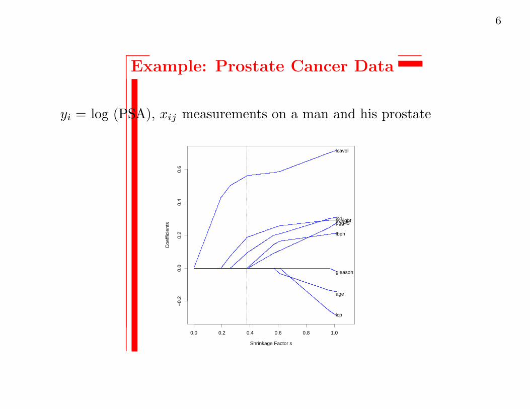
Example: Prostate Cancer Data

yi = log (PSA), xij measurements on a man and his prostate

Shrinkage Factor s

Coe

ffici

ents

0.0 0.2 0.4 0.6 0.8 1.0

−0.

20.

00.

20.

40.

6

lcavol

lweight

age

lbph

svi

lcp

gleason

pgg45

7

Estimated coefficients

Term Least Squares Ridge Lasso

Intercept 2.465 2.452 2.468

lcavol 0.680 0.420 0.533

lweight 0.263 0.238 0.169

age −0.141 −0.046

lbph 0.210 0.162 0.002

svi 0.305 0.227 0.094

lcp −0.288 0.000

gleason −0.021 0.040

pgg45 0.267 0.133

8

Emerging themes

• Lasso (ℓ1) penalties have powerful statistical and

computational advantages

• ℓ1 penalties provide a natural to encourage/enforce sparsity

and simplicity in the solution.

• “Bet on sparsity principle” (In the Elements of Statistical

learning). Assume that the underlying truth is sparse and use

an ℓ1 penalty to try to recover it. If you’re right, you will do

well. If you’re wrong— the underlying truth is not sparse—,

then no method can do well. [Bickel, Buhlmann, Candes,

Donoho, Johnstone,Yu ...]

• ℓ1 penalties are convex and the assumed sparsity can lead to

significant computational advantages

9

Outline

• New fast algorithm for lasso- Pathwise coordinate descent

• Examples of applications/generalizations of the lasso:

• Logistic/multinomial for classification. Example later

of classification from microarray data

• Degrees of freedom

• Near-isotonic regression - a modern take on an old idea

• Sparse principal components analysis

• More topics mentioned at end of talk

10

Algorithms for the lasso

• Standard convex optimizer

• Least angle regression (LAR) - Efron et al 2004- computes

entire path of solutions. State-of-the-Art until 2008

• Pathwise coordinate descent- new

11

Pathwise coordinate descent for the lasso

• Coordinate descent: optimize one parameter (coordinate) at a

time.

• How? suppose we had only one predictor. Problem is to

minimize ∑

i

(yi − xiβ)2 + λ|β|

• Solution is the soft-thresholded estimate

sign(β)(|β| − λ)+

where β is usual least squares estimate.

• Idea: with multiple predictors, cycle through each predictor in

turn. We compute residuals ri = yi −∑

k 6=j xikβk and applying

univariate soft-thresholding, pretending that our data is

(xij , ri).

12

Soft-thresholding

λ

β1

β2

β3

β4

13

• Turns out that this is coordinate descent for the lasso criterion∑

i

(yi −∑

j

xijβj)2 + λ

∑|βj |

• like skiing to the bottom of a hill, going north-south, east-west,

north-south, etc. [SHOW MOVIE]

• Too simple?!

14

A brief history of coordinate descent for the lasso

• 1997: Tibshirani’s student Wenjiang Fu at University of

Toronto develops the “shooting algorithm” for the lasso.

Tibshirani doesn’t fully appreciate it

• 2002 Ingrid Daubechies gives a talk at Stanford, describes a

one-at-a-time algorithm for the lasso. Hastie implements it,

makes an error, and Hastie +Tibshirani conclude that the

method doesn’t work

• 2006: Friedman is the external examiner at the PhD oral of

Anita van der Kooij (Leiden) who uses the coordinate descent

idea for the Elastic net. Friedman wonders whether it works for

the lasso. Friedman, Hastie + Tibshirani start working on this

problem. See also Wu and Lange (2008)!

15

Pathwise coordinate descent for the lasso

• Start with large value for λ (very sparse model) and slowly

decrease it

• most coordinates that are zero never become non-zero

• coordinate descent code for Lasso is just 73 lines of

Fortran!

16

Extensions

• Pathwise coordinate descent can be generalized to many other

models: logistic/multinomial for classification, graphical lasso

for undirected graphs, fused lasso for signals.

• Its speed and simplicity are quite remarkable.

• glmnet R package available on CRAN. Fits Gaussian,

Binomial/Logistic, Multinomial, Poisson, and Cox models.

17

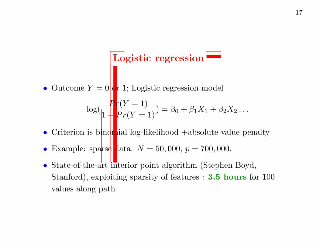
Logistic regression

• Outcome Y = 0 or 1; Logistic regression model

log(Pr(Y = 1)

1− Pr(Y = 1)) = β0 + β1X1 + β2X2 . . .

• Criterion is binomial log-likelihood +absolute value penalty

• Example: sparse data. N = 50, 000, p = 700, 000.

• State-of-the-art interior point algorithm (Stephen Boyd,

Stanford), exploiting sparsity of features : 3.5 hours for 100

values along path

18

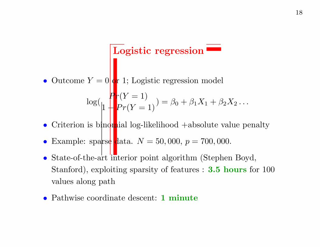
Logistic regression

• Outcome Y = 0 or 1; Logistic regression model

log(Pr(Y = 1)

1− Pr(Y = 1)) = β0 + β1X1 + β2X2 . . .

• Criterion is binomial log-likelihood +absolute value penalty

• Example: sparse data. N = 50, 000, p = 700, 000.

• State-of-the-art interior point algorithm (Stephen Boyd,

Stanford), exploiting sparsity of features : 3.5 hours for 100

values along path

• Pathwise coordinate descent: 1 minute

19

Multiclass classification

Microarray classification: 16,000 genes, 144 training samples 54 test

samples, 14 cancer classes. Multinomial regression model.

Methods CV errors Test errors # of

out of 144 out of 54 genes used

Support vector classifier 26 (4.2) 14 16063

Lasso-penalized multinomial 17 (2.8) 13 269

20

Degrees of freedom

• Let’s first consider all subset regression with total of p = 100

predictors.

• Suppose that we apply all-subset regression to obtain the best

subset of size k.

• Define the degrees of freedom DF of the fit as the average drop

in residual sum of squares divided by the error variance

• If we fit a fixed model with k predictors, DF = k.

• In all-subset selection, how many DF do we use, as a function

of k?

21

Quiz

0 20 40 60 80 100

020

4060

80

Number of predictors chosen

Deg

rees

of f

reed

om

A

0 20 40 60 80 100

040

8012

0


Deg

rees

of f

reed

om

B

0 20 40 60 80 100

020

4060

80


Deg

rees

of f

reed

om

C

0 20 40 60 80 100

020

4060

80


Deg

rees

of f

reed

om

D

22

DF for all subset regression

0 20 40 60 80 100

020

4060

8010

0


Deg

rees

of f

reed

om

Degrees of freedom is > k, since we selected the best k out of p

23

Degrees of freedom of the lasso

Some magic occurs...

• Define degrees of freedom using Efron’s formula,

DF =

n∑

i=1

cov(yi, yi)/σ2

• Apply Stein’s lemma:∑

icov(yi, yi)/σ

2 = E∑

i

dyidyi

• For the lasso fit y(k) having k non-zero predictors, this gives

DF(y(k)) ≈ k !!!!!!!!!!!!!!!!!

Although lasso chooses k predictors adaptively, the coefficients are

shrunken just the right amount to make DF equal to k!

[Efron, Hastie, Johnstone, Tibs]; [Zou, Hastie+Tibs]; [Ryan

Tibs+Taylor]

24

Near Isotonic regression

Ryan Tibshirani, Holger Hoefling, Rob Tibshirani (2010)

• generalization of isotonic regression: data sequence

y1, y2, . . . yn.

minimize∑

(yi − yi)2 subject to y1 ≤ y2 . . .

Solved by Pool Adjacent Violators algorithm.

• Near-isotonic regression:

βλ = argmin β∈Rn

1

2

n∑

i=1

(yi − βi)2 + λ

n−1∑

i=1

(βi − βi+1)+,

with x+ indicating the positive part, x+ = x · 1(x > 0).

25

Near-isotonic regression- continued

• Convex problem. Solution path βi = yi at λ = 0 and

culminates in usual isotonic regression as λ→∞. Along the

way gives near monotone approximations.

26

Numerical approach

How about using coordinate descent?

• Surprise! Although criterion is convex, it is not differentiable,

and coordinate descent can get stuck in the “cusps”

28

No improvement No improvement

Improvement

29

When does coordinate descent work?

Paul Tseng (1988), (2001)

If

f(β1 . . . βp) = g(β1 . . . βp) +∑

hj(βj)

where g(·) is convex and differentiable, and hj(·) is convex, then

coordinate descent converges to a minimizer of f .

Non-differential part of loss function must be separable

30

Solution: devise a path algorithm

• Simple algorithm that computes the entire path of solutions, a

modified version of the well-known pool adjacent violators

• Analogous to LARS algorithm for lasso in regression

• Bonus: we show that the degrees of freedom is the number of

“plateaus” in the solution. Using results from Ryan

Tibshirani’s PhD work with Jonathan Taylor

31

Toy example

λ = 0 λ = 0.25

λ = 0.7 λ = 0.77

32

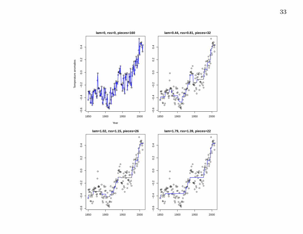
Global warming data

33

1850 1900 1950 2000

−0.

6−

0.4

−0.

20.

00.

20.

4

lam=0, rss=0, pieces=160

Year

Tem

pera

ture

ano

mal

ies

1850 1900 1950 2000

−0.

6−

0.4

−0.

20.

00.

20.

4

lam=0.44, rss=0.81, pieces=32

1850 1900 1950 2000

−0.

6−

0.4

−0.

20.

00.

20.

4


1850 1900 1950 2000

−0.

6−

0.4

−0.

20.

00.

20.

4


34

Penalized Matrix Decomposition

Daniela Witten, PhD thesis

Start with N × p data matrix X.

(u,v, d) = argmin ||X− duvT ||2F s.t. ||u||2 = ||v||2 = 1,

||u||1 ≤ c1, ||v||1 ≤ c2,

Useful for “sparsifying” a wide variety of multivariate procedures

(PCA, CCA, clustering)

Can write as argmax[uTXv] with same constraints.

35

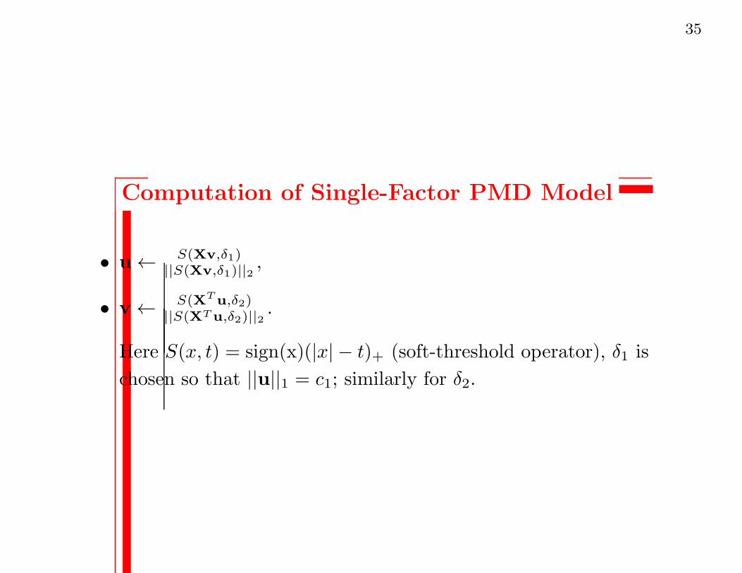
Computation of Single-Factor PMD Model

• u← S(Xv,δ1)||S(Xv,δ1)||2

,

• v← S(XTu,δ2)

||S(XTu,δ2)||2.

Here S(x, t) = sign(x)(|x| − t)+ (soft-threshold operator), δ1 is

chosen so that ||u||1 = c1; similarly for δ2.

36

• Generalizes power method for obtaining first singular vector;

• With c1 =∞, yields first sparse principal component v of

data.

• Criterion is not convex but is bi-convex

• Equivalent to ScotLass proposal of Jolliffe, Trendafilov and

Uddin, (2003)

37

Example: Corpus callosum shape study

569 elderly individuals: measurements of corpus collosum, walking

speed and verbal fluency

Figure 1: An example of a mid-aggital brain slice, with the corpus

collosum annotated with landmarks.

38

Walking Speed

Verbal Fluency

Principal Components Sparse Principal Components

39

Discussion

• lasso penalties are useful for fitting a wide variety of models

with sparsity constraints; pathwise coordinate descent enables

to fit these models to large datasets for the first time

• In CRAN: coordinate descent in R glmnet- linear regression,

logistic, multinomial, Cox model, Poisson

• Also: LARS, nearIso, cghFLasso, glasso

• PMA (penalized multivariate analysis) R package

• Matlab software for glm.net and matrix completion

http://www-stat.stanford.edu/∼ tibs/glmnet-matlab/

http://www-stat.stanford.edu/∼rahulm/SoftShrink

40

Ongoing work in lasso/sparsity

• grouped lasso (Yuan and Lin) and many variations

• multivariate- principal components, canonical correlation,

clustering (Witten and others)

• matrix-variate normal (Genevera Allen)

• Matrix completion- Candes, Mazumder, Hastie+Tibs

• graphical models, graphical lasso (Yuan+Lin, Friedman,

Hastie+Tibs, Mazumder, Witten, Simon; Peng, Wang et al)

• Compressed sensing (Candes and co-authors)

• “Strong rules” (Tibs et al 2010) provide a 5-80 fold speedup in

computation, with no loss in accuracy

• Interactions (Bien, Simon, Lim/Hastie)

41

Some challenges

• develop tools and theory that allow these methods to be used

in statistical practice: standard errors, p-values and confidence

intervals that account for the adaptive nature of the estimation.

• while it’s fun to develop these methods, as statisticians, our

ultimate goal is to provide better answers to scientific questions

41-1

References

the lasso: some novel algorithms and applicationsstatweb.stanford.edu/~tibs/ftp/lassotalk2.pdf ·...

Documents