the kernel trick
TRANSCRIPT

Seminar 1
The Kernel TrickEdgar Marca
Supervisor: DSc. André M.S. Barreto
Petrópolis, Rio de Janeiro - BrazilMay 21st and May 28th, 2015
1 / 125

The plan

The PlanGeneral Overview
3 / 125

The Plan1.- Kernel Methods
4 / 125
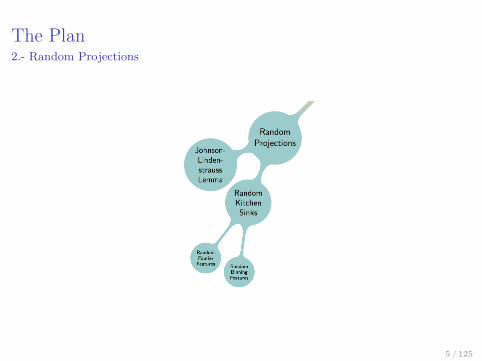
The Plan2.- Random Projections
5 / 125

The Plan3.- Deep Learning
6 / 125

The Plan4.- More about Kernels
7 / 125

The PlanMain Goal
The main goal of these set of seminars is to have enough theoreticalbackground to understand the following papers
I Julien Mairal et al., Convolutional Kernel Networks.I Quoc Viet Le et al., Fastfood: Approximate Kernel Expansions in
Loglinear Time.I Zichao Yang et al., Deep Fried Convnets.
8 / 125

Greetings
Part of the content of these slides was done in collaboration with mystudy group from the School of Mathematics at UNMSM (UniversidadNacional Mayor de San Marcos, Lima - Perú). I want to thank themembers of the group for the great conversations and fun time studyingSupport Vector Machines at the legendary office 308.
I DSc. Jose R. Luyo Sanchez (UNMSM).I Lic. Diego A. Benavides Vidal (Currently a Master Student at
UnB).I Bach. Luis E. Quispe Paredes (UNMSM).
Also, I want to thank DSc. André M.S. Barreto, my supervisor, for giveme the freedom to choose my topic of research. As soon as I finish withmy obligatory courses at LNCC, I will start working in ReinforcementLearning. :)
9 / 125

Table of Contents

Table of Contents IMotivation
R to R2 CaseR2 to R3 Case
Cover’s TheoremDefinitionsPreliminaries to Cover’s TheoremCover’s Theorem
References for Cover’s TheoremMercer’s Theorem
Theory of Bounded Linear OperatorsIntegral OperatorsPreliminaries to Mercer TheoremMercer’s Theorem
References for Mercer’s TheoremMoore-Aronszajn Theorem
Reproducing Kernel Hilbert Spaces11 / 125

Table of Contents IIMoore-Aronszajn Theorem
References for Moore-Aronszajn Theorem
Kernel TrickDefinitionsFeature Space based on Mercer’s Theorem
History
References
12 / 125

"Nothing is more practical than a good theory."
— From Vapnik’s preface to The Nature of Statistical Learning Theory
13 / 125

Motivation

Motivation
Motivation
I How we can split data that is not linear separable?I How we can utilize algorithms that works for linear separable data
that only depends on the inner product?
15 / 125

Motivation R to R2 Case
R to R2 CaseHow to separate two classes?
0
R
R2
ϕ(x) = (x, x2)
ϕ
Figure: Separating the two classes of points by tranforming the points into ahigher dimensional space where the data is separable.
16 / 125

Motivation R2 to R3 Case
R2 to R3 Case
+
+
+
+
+
+
+
+
++
+
+
+
+
+
-
-
-
-
-
-
-
-
-
-
- -
-
-
-
-
-
-
-
-
-
--
-
-
-
-
-
-
--
-
-
--
-
-
-
Figure: Data which is not linear separable.17 / 125

Motivation R2 to R3 Case
R2 to R3 CaseA simulation
Figure: SVM with polynomial kernel visualization.
18 / 125

Motivation R2 to R3 Case
ϕ
ϕ(+)ϕ(+)
ϕ(+)
ϕ(−)
ϕ(−)
ϕ(−)
ϕ(−)
ϕ(−)
ϕ(+)ϕ(+)
Figure: ϕ is a non-linear mapping from the input space to the feature space.
19 / 125

Cover’s Theorem

Cover’s Theorem Definitions
During this section we will consider X a finite subset of Rd
X = x1, x2, . . . , xN (1)
where N a fixed natural number and xi in Rd for all 1 ≤ i ≤ N
21 / 125

Cover’s Theorem Definitions
Definition 2.1 (Homogenous Linear Threshold Function)Consider a set of patterns represented by a set of vectors in ad-dimensional Euclidean space Rd. A homogeneously linear thresholdfunction is defined in terms of a parameter vector w for every vector xin Rd as
fw : Rd → −1, 0, 1
x 7→ fw(x) =
1, If 〈w, x〉 > 0
0, If 〈w, x〉 = 0
−1, If 〈w, x〉 < 0
Note: The function fw can be written as fw(x) = sign(〈w, x〉).
22 / 125

Cover’s Theorem Definitions
Thus every homogeneous linear threshold function naturally divides Rdinto two sets, the set of vectors x such that fw(x) = 1 and the set ofvectors x such that fw(x) = −1. These two sets are separated by thehyperplane
H = x ∈ Rd | fw(x) = 0 = x ∈ Rd | 〈w, x〉 = 0 (2)which is the (d− 1)-dimensional subspace orthogonal to the weightvector w.
w 〈w, x〉 = 0
Figure: Some points of Rd divided by an homogeneous linear thresholdfunction.
23 / 125

Cover’s Theorem Definitions
Definition 2.2 (Linearly Separable Dichotomies)A dichotomy X+, X−, a binary partition1, of X is linearly separableif and only if there exists a weight vector w in Rd and scalar b 6= 0 suchthat
〈w, x〉 > b, if x ∈ X+
〈w, x〉 < b, if x ∈ X−
Definition 2.3 (Homogeneously Linearly Separable Dichotomies)Let X be an arbitrary set of vectors in Rd. A dichotomy X+, X−, abinary partition, of X is homogeneously linearly separable if and only ifthere exists a weight vector w in Rd such that
〈w, x〉 > 0, if x ∈ X+
〈w, x〉 < 0, if x ∈ X−
1X = X+ ∪X− and X+ ∩X− = ∅.24 / 125

Cover’s Theorem Definitions
Definition 2.4 (Vectors in General Position)Let X be an arbitrary set of vectors in Rd. A set of N vectors is ingeneral position in d-space if every subset of d or fewer vectors arelinearly independent.
Figure: Left: A set of vectors that are not in general position. Right: A setof vectors that are in general position.
25 / 125

Cover’s Theorem Preliminaries to Cover’s Theorem
Lemma 2.5Let X− and X+ subsets of Rd, and let y a point other than the originin Rd. Then the dichotomies X+ ∪ y, X− and X+, X− ∪ y areboth homogeneously linear separable if and only if X+, X− ishomogeneously linear separable by a (d− 1)-dimensionalsubspace2containing y.
Proof.Let W the set of separable vectors for X+, X− given by
W =w ∈ Rd | 〈w, x〉 > 0, x ∈ X+ ∧ 〈w, x〉 < 0, x ∈ X−
(3)
The set W can be rewritten as
W =w ∈ Rd | 〈w, x〉 > 0, x ∈ X+
⋂w ∈ Rd|〈w, x〉 < 0, x ∈ X−
(4)
2(d− 1)−dimensional subspace is an hyperplane.26 / 125

Cover’s Theorem Preliminaries to Cover’s Theorem
y
w1
w2
w∗
Figure: We construct a hyperplane passing thought y which vector weight isw∗ = 〈−〈w2, y〉w1 + 〈w1, y〉w2.
27 / 125

Cover’s Theorem Preliminaries to Cover’s Theorem
The dichotomy X+ ∪ y, X− is homogeneously separable if and onlyif there is a vector w in W such that 〈w, y〉 > 0 and the dichotomyX+, X− ∪ y is homogeneously linearly separable if and only if thereis a w in W such that 〈w, y〉 < 0.If X+ ∪ y, X− and X+, X− ∪ y are homogeneously separableby w1 and w2 respectively, then we can construct a w∗ as
w∗ = −〈w2, y〉w1 + 〈w1, y〉w2 (5)
such that separates X+, X− by the hyperplaneH = x ∈ Rd | 〈w∗, x〉 = 0 passing thought y. We affirm that ybelongs to H. Indeed,
〈w∗, y〉 = 〈−〈w2, y〉w1 + 〈w1, y〉w2, y〉= −〈w2, y〉〈w1, y〉+ 〈w1, y〉〈w2, y〉= 0
28 / 125

Cover’s Theorem Preliminaries to Cover’s Theorem
We affirm that 〈w∗, x〉 > 0 if x in X+. In fact, let x in X+ then
〈w∗, x〉 = 〈−〈w2, y〉w1 + 〈w1, y〉w2, x〉= −〈w2, y〉︸ ︷︷ ︸
>0
〈w1, x〉︸ ︷︷ ︸>0
+ 〈w1, y〉︸ ︷︷ ︸>0
〈w2, x〉︸ ︷︷ ︸>0
> 0
then 〈w∗, x〉 > 0 for all x in X+.We affirm that 〈w∗, x〉 < 0 if x in X−. In fact, let x in X− then
〈w∗, x〉 = 〈−〈w2, y〉w1 + 〈w1, y〉w2, x〉= −〈w2, y〉︸ ︷︷ ︸
<0
〈w1, x〉︸ ︷︷ ︸>0
+ 〈w1, y〉︸ ︷︷ ︸>0
〈w2, x〉︸ ︷︷ ︸<0
< 0
then 〈w∗, x〉 < 0 for all x in X−.We conclude that X+, X− is homogeneously separable by the vectorw∗.
29 / 125

Cover’s Theorem Preliminaries to Cover’s Theorem
Conversely, if X+, X− is homogeneously linear separable by anhypeplane containing y then there exists w∗ in W such that 〈w∗, y〉 = 0.We affirm that W is an open set. In fact, the set W can be rewritten as
W =
⋂x∈X+
w ∈ Rd | 〈w, x〉 > 0
⋂ ⋂x∈X−
w ∈ Rd | 〈w, x〉 < 0
(6)
and the complement of this set is
W c =
⋃x∈X+
w ∈ Rd | 〈w, x〉 ≤ 0
⋃ ⋃x∈X−
w ∈ Rd | 〈w, x〉 ≥ 0
(7)
The sets w ∈ Rd | 〈w, x〉 ≤ 0, x ∈ X+ andw ∈ Rd | 〈w, x〉 ≥ 0, x ∈ X− are clearly closed due to the continuityof the inner product then the finite union of closed sets is closed so wecan conclude that the set W c is closed therefore W is an open set.
30 / 125
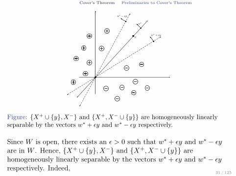
Cover’s Theorem Preliminaries to Cover’s Theorem
y
w∗ − ǫy
w∗ + ǫy
w∗
Figure: X+ ∪ y, X− and X+, X− ∪ y are homogeneously linearlyseparable by the vectors w∗ + εy and w∗ − εy respectively.
Since W is open, there exists an ε > 0 such that w∗ + εy and w∗ − εyare in W . Hence, X+ ∪ y, X− and X+, X− ∪ y arehomogeneously linearly separable by the vectors w∗ + εy and w∗ − εyrespectively. Indeed,
31 / 125

Cover’s Theorem Preliminaries to Cover’s Theorem
We will prove that X+ ∩ y, X− is homegenously linear separableby w∗ + εy.We affirm that 〈w∗ + εy, y〉 > 0. In fact,
〈w∗ + εy, y〉 = 〈w∗, y〉︸ ︷︷ ︸=0
+ε〈y, y〉 (8)
= ε‖y‖2 (9)> 0 (10)
Therefore, 〈w∗ + εy, y〉 > 0. Hence, X+ ∪ y, X− is homogeneouslylinearly separable by w∗ + εy.
32 / 125

Cover’s Theorem Preliminaries to Cover’s Theorem
We will prove that X+, X− ∩ y is homegenously linear separableby w∗ − εy. We affirm that 〈w∗ − εy, y〉 < 0. In fact,
〈w∗ + εy, y〉 = 〈w∗, y〉︸ ︷︷ ︸=0
+ε〈y, y〉 (11)
= −ε‖y‖2 (12)< 0 (13)
Therefore, 〈w∗ + εy, y〉 < 0. Hence, X+, X− ∪ y is homogeneouslylinearly separable by w∗ − εy.
33 / 125

Cover’s Theorem Preliminaries to Cover’s Theorem
Lemma 2.6A dichotomy of X separable by w if and only if the projection of the setX onto the (d− 1)-dimensional orthogonal subspace to y is separable.
Proof.Exercise :) (Intuitively it works but I don’t have an algebraic proof yet.)
y
w
X+
X−
Figure: Projecting the sets X+ and X− to the hyperplane orthogonal to thehyperplane passing thought y.
34 / 125
Cover’s Theorem Preliminaries to Cover’s Theorem
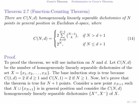
Theorem 2.7 (Function-Counting Theorem)There are C(N, d) homogeneously linearly separable dichotomies of Npoints in general position in Euclidean d-space, where
C(N, d) =
2d−1∑k=0
(N−1k
), if N > d+ 1
2N , if N ≤ d+ 1
(14)
Proof.To proof the theorem, we will use induction on N and d. Let C(N, d)be the number of homogeneously linearly separable dichotomies of theset X = x1, x2, . . . , xN. The base induction step is true becauseC(1, d) = 2 if d ≥ 1 and C(N, 1) = 2 if N ≥ 1. Now, let’s prove thatthe theorem is true for N + 1 points. Consider a new point xN+1 suchthat X ∪ xN+1 is in general position and consider the C(N, d)homogeneously linearly separable dichotomies X+, X− of X.
35 / 125

Cover’s Theorem Preliminaries to Cover’s Theorem
Since X+, X− is separable, either X+ ∪ xN+1, X− orX+, X− ∪ xN+1. However, both dichotomies are separable, bylemma (2.5), if and only if exists a separating vector w for X+, X−lying in the (d− 1)-dimensional subspace orthogonal to xN+1. Adichotomy of X is separable by such a w if and only if the projection ofthe set X onto the (d− 1)-dimensional orthogonal subspace to xN+1 isseparable. By the induction hypothesis there are C(N, d− 1) suchseparable dichotomies. Hence
C(N + 1, d) = C(N, d)︸ ︷︷ ︸Number of Homogeneously Linearlyseparable dichotomies of N points
in general position in Euclidean d-space
+ C(N, d− 1)︸ ︷︷ ︸Number of Homogeneously Linearlyseparable dichotomies of N pointsin general position d − 1-subspace
36 / 125

Cover’s Theorem Preliminaries to Cover’s Theorem
C(N + 1, d) = C(N, d) + C(N, d− 1)
= 2
(d−1∑k=0
(N − 1
k
)+
d−2∑k=0
(N − 1
k
))
= 2
((N − 1
0
)+
d−1∑k=1
((N − 1
k
)+
(N − 1
k − 1
)))
= 2
((N
0
)+
d−1∑k=1
(N
k
))
= 2
d−1∑k=0
(N
k
)
37 / 125

Cover’s Theorem Preliminaries to Cover’s Theorem
therefore,
C(N, d) = 2
d−1∑k=0
(N − 1
k
)(15)
38 / 125

Cover’s Theorem Cover’s Theorem
Two kinds of randomness are considered in the pattern recognitionproblem:
I The pattern are fixed in position but are classified independentlywith equal probability into one of two categories.
I The patterns themselves are randomly distributed in space, andthe desired dichotomization maybe random or fixed.
Suppose that the dichotomy of X = x1, x2, . . . , xN is chosen arerandom with equal probability from the 2N equiprobable possibledichotomies of X.Let P (N, d) be the probability that the random dichotomy is linearseparable.
P (N, d) =C(N, d)
2N=
(12
)N−1 d−1∑k=0
(N−1k
), if N > d+ 1
1, if N ≤ d+ 1
(16)
39 / 125

Cover’s Theorem Cover’s Theorem
Figure: Behaviour of the probability P (N, d) vs Nd+1 [12, p.46].
I If Nd+1 ≤ 1 then P (N, d+ 1) = 1.
I If 1 < Nd+1 < 2 and d→∞ then P (N, d+ 1)→ 1.
I If Nd+1 = 2 then P (N, d+ 1) = 1
2 .
40 / 125

Cover’s Theorem Cover’s Theorem
Theorem 2.8 (Cover’s Theorem)A complex pattern classification problem cast in a high-dimensionalspace nonlinearly, is more likely to be linearly separable than in alow-dimensional space.
41 / 125

References for Cover’s Theorem
References for Cover’s TheoremMain Source:
[7] Thomas Cover. “Geometrical and Statistical properties of systemsof linear inequalities with applications in pattern recognition”. In:IEEE Transactions on Electronic Computer (), pp. 326–334.
Minor Sources:
[12] Ke-Lin Du and M. N. S. Swamy. Neural Networks and StatisticalLearning. Springer Science & Business Media, 2013.
[19] Simon Haykin. Neural Networks and Learning Machines. ThirdEdition. Pearson Prentice Hall, 2009.
[39] Bernhard Schlköpf and Alexander Smola. Learning with Kernels:Support Vector Machines, Regularization, Optimization, andBeyond. The MIT Press, 2001.
[49] Sergios Theodoridis. Machine Learning: A Bayesian andOptimization Perspective. Academic Press, 2015.
42 / 125

Mercer’s Theorem

Mercer’s Theorem Integral Operators
Theorem 6.1 (Teorema de Mercer)Let k a continous function in [a, b]× [a, b] such that∫ b
a
∫ b
ak(t, s)f(s)f(t) ds dt ≥ 0 (17)
for all f in L2([a, b]), then, for all t and s in [a, b] the series
k(t, s) =
∞∑j=1
λjϕj(t)ϕj(s)
converges absolutely and uniformly in the set [a, b]× [a, b].
44 / 125

Mercer’s Theorem Integral Operators
Integral Operators
Definition 6.2 (Integral Operador)Let k a measurable function in the set [a, b]× [a, b], then the integraloperator K associated to the function k is defined by
K : Γ→ Ω
f 7→ (Kf)(t) :=
∫ b
ak(t, s)f(s) ds
where Γ and Ω are space of functions. This operator is well definedwhenever the integral exists.
45 / 125

Mercer’s Theorem Integral Operators
Theorem 6.3Let k a measurable complex Lebesgue function in L2([a, b]× [a, b]) andlet K the integral operator associated to the function k defined by
K : L2 ([a, b])→ L2 ([a, b])
f 7→ (Kf)(t) =
∫ b
ak(t, s)f(s) ds
then the following affirmations are hold1. The integral exists.2. The integral operator associated to k is well defined.3. The integral operator associated to k is linear.4. The integral operator associated to k is a bounded operator.
Skip Proof
46 / 125

Mercer’s Theorem Integral Operators
Proof.1. The integral exists because for almost every s in [a, b] the functionsk(t, .) and f(.) are Lebesgue measurable functions in [a, b].2. To proof that the integral operator K is well defined we have toshow that the image of the operator is contained in L2([a, b]). Indeed,because k is in L2([a, b]× [a, b]) then
‖k‖2L2([a,b]×[a,b]) =
∫ b
a
∫ b
a|k(t, s)|2 ds dt <∞ (18)
on the other hand,
47 / 125

Mercer’s Theorem Integral Operators
Proof.
‖Kf‖2L2([a,b]) = 〈Kf,Kf〉L2([a,b])
=
∫ b
a(Kf)(t)(Kf)(t) dt
=
∫ b
a
(∫ b
ak(t, s)f(s) ds
)(∫ b
ak(t, s)f(s) ds
)dt
=
∫ b
a
∣∣∣∣∫ b
ak(t, s)f(s) ds
∣∣∣∣2 dt≤∫ b
a
(∫ b
a|k(t, s)f(s)| ds
)2
dt
≤∫ b
a
[(∫ b
a|k(t, s)|2 ds
)(∫ b
a|f(s)|2 ds
)]dt (D. C-S)
48 / 125

Mercer’s Theorem Integral Operators
=
(∫ b
a|f(s)|2 ds
)(∫ b
a
∫ b
a|k(t, s)|2 ds dt
)= ‖f‖2L2([a,b])
∫ b
a
∫ b
a|k(t, s)|2 ds dt
= ‖f‖2L2([a,b])‖k‖2L2([a,b]×[a,b])
then‖Kf‖2L2([a,b]) ≤ ‖f‖2L2([a,b])‖k‖2L2([a,b]×[a,b]) (19)
using the previous inequality (19), by eq. (18) and due to f in L2([a, b])we conclude
49 / 125

Mercer’s Theorem Integral Operators
‖Kf‖2L2([a,b]) ≤ ‖f‖2L2([a,b])‖k‖2L2([a,b]×[a,b]) <∞ (20)
therefore, the functions Kf is in L2([a, b]) and we can conclude that theintegral operator K is well defined.3. Let α, β in R an f , g in L2([a, b]) then
K(αf + βg) =
∫ b
a[k(t, s)(αf(s) + βg(s))]ds
= α
∫ b
ak(t, s)f(s)ds+ β
∫ b
ak(t, s)g(s)ds
= αK(f) + βK(g)
therefore the integral operator K is a linear operator.
50 / 125
Mercer’s Theorem Integral Operators
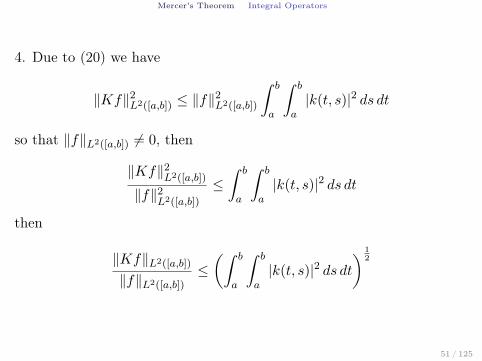
4. Due to (20) we have
‖Kf‖2L2([a,b]) ≤ ‖f‖2L2([a,b])
∫ b
a
∫ b
a|k(t, s)|2 ds dt
so that ‖f‖L2([a,b]) 6= 0, then
‖Kf‖2L2([a,b])
‖f‖2L2([a,b])
≤∫ b
a
∫ b
a|k(t, s)|2 ds dt
then
‖Kf‖L2([a,b])
‖f‖L2([a,b])≤(∫ b
a
∫ b
a|k(t, s)|2 ds dt
) 12
51 / 125

Mercer’s Theorem Integral Operators
‖K‖ = sup‖f‖L2([a,b]) 6=0
‖Kf‖L2([a,b])
‖f‖L2([a,b])
≤(∫ b
a
∫ b
a|k(t, s)|2 ds dt
) 12
= ‖k‖L2([a,b]×[a,b]) <∞
in the last inequality using the equation (18) we can conclude that‖K‖ <∞ so K is a bounded operator.
52 / 125

Mercer’s Theorem Integral Operators
Corollary 6.4If k is a continuous measurable Lebesgue complex function in[a, b]× [a, b] then the integral operator associated to k is inL(L2([a, b]), L2([a, b])).
Proof.As k is a continuous function then |k(t, s)| is a continuous function.Moreover, every continuous function in a compact set [a, b]× [a, b] isbounded then k en L2([a, b]× [a, b]).
53 / 125

Mercer’s Theorem Integral Operators
Lemma 6.5Let ϕ1, ϕ2, . . . an orthonormal basis for L2([a, b]), the function definedas Φij(s, t) = ϕi(s)ϕj(t), for all i, j in N is an orthonormal basis forL2([a, b]× [a, b]).
Proof.We affirm that the set B = Φij | ∀i, j ∈ N is orthonormal, in fact
〈Φjk,Φmn〉L2([a,b]×[a,b]) =
∫ b
a
∫ b
aϕj(s)ϕk(t)ϕm(s)ϕn(t) ds dt
=
∫ b
a
∫ b
aϕj(s)ϕk(t)ϕm(s)ϕn(t) ds dt
54 / 125

Mercer’s Theorem Integral Operators
〈Φjk,Φmn〉L2([a,b]×[a,b]) =
∫ b
a
∫ b
aϕj(s)ϕk(t)ϕm(s)ϕn(t) ds dt
=
∫ b
a
∫ b
aϕj(s)ϕk(t)ϕm(s)ϕn(t) ds dt
=
∫ b
aϕj(s)ϕm(s) ds
∫ b
aϕk(t)ϕn(t) dt
(T. Fubini)
= δjmδkn
where
δjmδkn =
1, if j = m ∧ k = n
0, in other case(21)
therefore B is an orthonormal set.
55 / 125

Mercer’s Theorem Integral Operators
We affirm that B is a basis. To show that B is a basis we have to proofif g is in L2 ([a, b]× [a, b]) and 〈g,Φjk〉L2([a,b]×[a,b]) = 0, this implies thatg ≡ 0 almost everywhere this is because theorem ?? (2) then we canconclude that B is an orthonormal basis for L2([a, b]× [a, b]). Indeed,Let g in L2([a, b]× [a, b]), then
0 = 〈g,Φjk〉L2([a,b]×[a,b]) =
∫ b
a
∫ b
ag(s, t)ϕj(s)ϕk(t) ds dt
=
∫ b
aϕj(s)
∫ b
ag(s, t)ϕk(t) dt︸ ︷︷ ︸
h
ds
=
∫ b
aϕj(s)h ds
=
∫ b
ahϕj(s) ds
= 〈h, ϕj〉L2([a,b])56 / 125

Mercer’s Theorem Integral Operators
then
〈h, ϕj〉L2([a,b]) = 0 (22)
where the function h is
h(s) =
∫ b
ag(s, t)ϕk(t) dt
the function h can be written in the following form
h(s) = 〈g(s, .), ϕk〉L2([a,b]) , ∀k = 1, 2, . . . (23)
as the function h is orthonormal to every function ϕj this implies thath ≡ 0 in almost every point s in [a, b] (theorem ?? (2)). By theequation (23) and h ≡ 0 we can conclude that there is a set Ω whichmeasure is zero such that for all s which is not in Ω the function g(s, .)is orthogonal to ϕk for all k = 1, 2, . . . therefore g(s, t) = 0 for all t andeach s which doesn’t belongs to Ω (theorem ?? (2)). Therefore
57 / 125
Mercer’s Theorem Integral Operators
∫ b
a
∫ b
a|g(s, t)|2 dt ds = 0
so we conclude g ≡ 0 almost in everywhere point (t, s) in [a, b]× [a, b].This proof that the set B is an orthonormal basis for L2([a, b]× [a, b]).
58 / 125

Mercer’s Theorem Integral Operators
Theorem 6.6Let k a function defined in L2([a, b]× [a, b]) and let K the integraloperator associated to the function k defined as
K : L2 ([a, b])→ L2 ([a, b])
f 7→ (Kf)(t) =
∫ b
ak(t, s)f(s) ds
then the adjoint opeator K∗ of the integral operator K is given by
(K∗g)(t) =
∫ b
ak(s, t)g(s) ds
for all g in L2([a, b]).
59 / 125

Mercer’s Theorem Integral Operators
Proof.
〈Kf, g〉L2([a,b]) =
∫ b
a(Kf(t)) g(t) dt
=
∫ b
a
(∫ b
ak(t, s)f(s) ds
)g(t) dt
=
∫ b
a
(∫ b
ak(t, s)f(s)g(t) ds
)dt
=
∫ b
a
(∫ b
ak(t, s)f(s)g(t) dt
)ds (T. Fubini)
=
∫ b
af(s)
(∫ b
ak(t, s)g(t) dt
)ds
=
∫ b
af(s)
(∫ b
ak(t, s)g(t) dt
)ds
= 〈f,K∗g〉L2([a,b])
60 / 125

Mercer’s Theorem Integral Operators
where K∗g is defined by
K∗g(s) :=
∫ b
ak(t, s)g(t) dt
is the auto-adjoint operator of K.
61 / 125

Mercer’s Theorem Integral Operators
Theorem 6.7Let k a function in L2([a, b]× [a, b]) and let K the integral operatorassociated to k defined as
K : L2 ([a, b]× [a, b])→ L2 ([a, b])
f 7→ (Kf)(t) =
∫ b
ak(t, s)f(s) ds
then the integral operator K is a compact operator.Skip Proof
62 / 125

Mercer’s Theorem Integral Operators
Proof.During this proof we will write 〈k,Φij〉 instead of 〈k,Φij〉L2([a,b]×[a,b]).First of all, we will build a sequence of operator with finite range whichconverges in norm to the integral operator K as follows:Let ϕ1, ϕ2, . . . an orthonormal basis for L2 ([a, b]). Then, the functionsdefined by
Φij(t, s) = ϕi(t)ϕj(s) ∀i, j = 1, 2, . . .
, by lemma 6.5 this functions form an orthonormal basis forL2 ([a, b]× [a, b]).The function k by the lemma ?? (2) can be written as
k(t, s) =
∞∑i=1
∞∑j=1
〈k,Φij〉Φij(t, s)
and we defined a sequence of functions kn∞n=1, where the n-thfunction is defined as
63 / 125

Mercer’s Theorem Integral Operators
kn(t, s) :=
n∑i=1
n∑j=1
〈k,Φij〉Φij(t, s)
then the sequence k − kn∞n=1 converge to 0 in norm inL2([a, b]× [a, b]) i.e.
limn→∞
‖k − kn‖L2([a,b]×[a,b]) = 0
which is equivalent in notation to
‖k − kn‖L2([a,b]×[a,b]) → 0 (24)
on the other hand, let Kn the integral operador associated to thefunction kn defined in L2 ([a, b]) as
(Knf)(t) :=
∫ b
akn(t, s)f(s) ds
Kn is a bounded operator64 / 125

Mercer’s Theorem Integral Operators
(due to kn is a linear combination of functions in L2([a, b]), a vectorspace, and by theorem (6.3) we can conclude that the operador islinear and bounded) with finite range because Kn is inspanϕ1, . . . , ϕn, in fact
(Knf)(t) =
∫ b
akn(t, s)f(s) ds
=
∫ b
a
n∑i=1
n∑j=1
〈k,Φij〉Φij(t, s)
f(s) ds
=
∫ b
a
n∑i=1
n∑j=1
〈k,Φij〉Φij(t, s)f(s) ds
=
n∑i=1
n∑j=1
(∫ b
a〈k,Φij〉Φij(t, s)f(s) ds
)
65 / 125

Mercer’s Theorem Integral Operators
=
n∑i=1
n∑j=1
(∫ b
a〈k,Φij〉ϕi(t)ϕj(s)f(s) ds
)
=
n∑i=1
n∑j=1
ϕi(t)
(∫ b
a〈k,Φij〉ϕj(s)f(s) ds
)
=
n∑i=1
ϕi(t)
n∑j=1
(∫ b
a〈k,Φij〉ϕj(s)f(s) ds
)
=
n∑i=1
ϕi(t)
∫ b
a
n∑j=1
(〈k,Φij〉ϕj(s)f(s)
)ds
66 / 125

Mercer’s Theorem Integral Operators
=
n∑i=1
∫ b
a
n∑j=1
〈k,Φij〉ϕj(s)f(s)
ds
︸ ︷︷ ︸αi
ϕi(t)
=
n∑i=1
αiϕi(t)
where
αi =
∫ b
a
n∑j=1
〈k,Φij〉ϕj(s)f(s)
ds ∀1 ≤ i ≤ n
so Kn in spanϕ1, . . . , ϕn hence the operator Kn is an operator withfinite range.
67 / 125

Mercer’s Theorem Integral Operators
On the other hand, because the operador K is linear and bounded then
‖K‖ ≤(∫ b
a
∫ b
a|k(t, s)|2 ds dt
) 12
= ‖k‖L2([a,b]×[a,b]) (25)
By the equation (25) applied to the operator K −Kn we have
‖K −Kn‖ ≤ ‖k − kn‖L2([a,b]×[a,b])
and by the equation (24) we have
‖K −Kn‖ ≤ ‖k − kn‖L2([a,b]×[a,b]) → 0
so we can conclude that
‖K −Kn‖ → 0
and applying the theorem ?? (puesto Kn es un operador de rangofinito) to the last equation we can conclude that the operator K is acompact operator.
68 / 125

Mercer’s Theorem Preliminaries to Mercer Theorem
Lemma 6.8Let k a continuous complex function defined in [a, b]× [a, b] which holds∫ b
a
∫ b
ak(t, s)f(s)f(t) ds dt ≥ 0 (26)
for all f in L2([a, b]) then the following statements are hold
1. The integral operator associated to k is a positive operator.2. The integral operator associated to k is an auto-adjoint operator.3. The number k(t, t) is real for all t in [a, b].4. The number k(t, t) holds k(t, t) ≥ 0, for all t in [a, b].
69 / 125

Mercer’s Theorem Preliminaries to Mercer Theorem
Lemma 6.9If k is a continuous complex function in [a, b]× [a, b] then the functionh defined as follows
h(t) =
∫ b
ak(t, s)ϕ(s) ds (27)
is continuous in [a, b] for all ϕ in L2([a, b]).
70 / 125

Mercer’s Theorem Preliminaries to Mercer Theorem
Lemma 6.10Let fn∞n=1 a sequence of continous real functions in [a, b] such thatsatisfies the next conditions:
1. f1(t) ≤ f2(t) ≤ f3(t) ≤ ... for all t in [a, b] (fn∞n=1 is amonotonous increasing sequence of functions).
2. f(t) = limn→∞
fn(t) is a continous function in [a, b].
and we define the set Fn as
Fn := t | f(t)− fn(t) ≥ ε ,∀n ∈ N
then
1. Fn+1 ⊂ Fn for all n in N.2. The set Fn is closed.
3.∞⋂n=1
Fn = ∅ .
71 / 125

Mercer’s Theorem Preliminaries to Mercer Theorem
Theorem 6.11 (Dini’s Theorem)Let fn∞n=1 a sequence of continous real functions in [a, b] such thatsatisfies the next conditions:
1. f1(t) ≤ f2(t) ≤ f3(t) ≤ ... for all t ∈ [a, b] (fn∞n=1 is amonotonous increasing sequence of functions).
2. f(t) = limn→∞
fn(t) es continua en [a, b].
Then the sequence of functions fn∞n=1 converges uniformently to thefunction f in [a, b].
72 / 125

Mercer’s Theorem Mercer’s Theorem
Theorem 6.12 (Teorema de Mercer)Let k a continous function in [a, b]× [a, b] such that∫ b
a
∫ b
ak(t, s)f(s)f(t) ds dt ≥ 0 (28)
for all f in L2([a, b]), then, for all t and s in [a, b] the series
k(t, s) =
∞∑j=1
λjϕj(t)ϕj(s)
converges absolutely and uniformly in the set [a, b]× [a, b].Skip Proof
73 / 125

Mercer’s Theorem Mercer’s Theorem
Proof.Applying Cauchy-Schwarz inequality to the set of functions√
λmϕm(t),√λmϕm(t), . . . ,
√λnϕn(t)
and √
λmϕm(s),√λmϕm(s), . . . ,
√λnϕn(s)
we have
n∑j=m
|λjϕj(t)ϕj(s)| ≤
n∑j=m
λj |ϕj(t)|2 1
2 n∑j=m
λj |ϕj(s)|2 1
2
(29)
Fixing t = t0 and by lemma ?? (5) applied to the seriesn∑
j=mλj |ϕj(t0)|2
given ε2 > 0 implies the existence of an integer N such that for all n, mn > m ≥ N satifies
74 / 125

Mercer’s Theorem Mercer’s Theorem
n∑j=m
λj |ϕj(t0)ϕj(s)| ≤
n∑j=m
λj |ϕj(t0)|2 1
2
︸ ︷︷ ︸<ε
n∑j=m
λj |ϕj(s)|2 1
2
︸ ︷︷ ︸≤C
< εC
, ∀s ∈ [a, b] where C2 = maxt∈[a,b]
k(t, t) and by Cauchy’s criteria for
uniform series we conclude that∞∑j=1
λjϕj(t)ϕj(s) converges absolutely
and uniformently in s for each t (t0 was arbitrary).
The next step is to prove that the series∞∑j=1
λjϕj(t)ϕj(s) converges to
k(t, s). Indeed, let k(t, s) the function defined by
k(t, s) :=
∞∑j=1
λjϕj(t)ϕj(s)
75 / 125

Mercer’s Theorem Mercer’s Theorem
and let the function f defined in L2 ([a, b]) and t = t0 fixed, the uniformconvergence of the series in s and the continuity of each function ϕj(because ϕj is a continous function) implies that k(t0, s) is continous asa function of s. Moreover, Let
LHS =
∫ b
a
[k(t0, s)− k(t0, s)
]f(s) ds
then
LHS =
∫ b
ak(t0, s)f(s) ds−
∫ b
ak(t0, s)f(s) ds
= (Kf)(t0)−∫ b
a
∞∑j=1
λjϕj(t0)ϕj(s)
f(s) ds
= (Kf)(t0)−∫ b
a
∞∑j=1
λjϕj(t0)ϕj(s)f(s)
ds
= (Kf)(t0)−∞∑j=1
(∫ b
aλjϕj(t0)ϕj(s)f(s) ds
)(T. Serie e integral)
76 / 125

Mercer’s Theorem Mercer’s Theorem
= (Kf)(t0)−∞∑j=1
λjϕj(t0)
(∫ b
aϕj(s)f(s) ds
)
= (Kf)(t0)−∞∑j=1
λjϕj(t0)
(∫ b
af(s)ϕj(s) ds
)
= (Kf)(t0)−∞∑j=1
λjϕj(t0)〈f, ϕj〉
= (Kf)(t0)−∞∑j=1
λj〈f, ϕj〉ϕj(t0)
=
∞∑j=1
λj〈f, ϕj〉ϕj(t0)−∞∑j=1
λj〈f, ϕj〉ϕj(t0)
= 0
77 / 125

Mercer’s Theorem Mercer’s Theorem
Therefore, k(t0, s) = k(t0, s) almost everywhere for s in [a, b]. Ask(t0, s) and k(t0, s) are continous then k(t0, s) = k(t0, s) for all s in [a, b]therefore k(t0, .) = k(t0, .) and as t0 was arbitrary then k ≡ k so that
k(t, s) = k(t, s) =
∞∑j=1
λjϕj(t)ϕj(s)
In particular, k(t, t) =∞∑j=1
λj |ϕj(t)|2 for all t in [a, b] and applying
Dini’s Theorem 6.11 to the functions
fn(t) =
n∑j=1
λj |ϕj(t)|2
78 / 125
Mercer’s Theorem Mercer’s Theorem
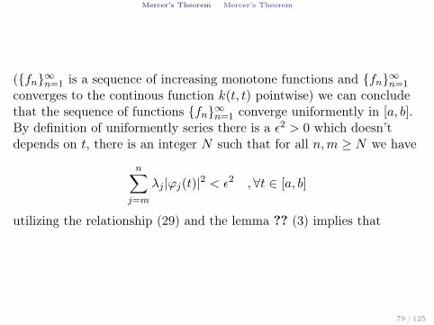
(fn∞n=1 is a sequence of increasing monotone functions and fn∞n=1
converges to the continous function k(t, t) pointwise) we can concludethat the sequence of functions fn∞n=1 converge uniformently in [a, b].By definition of uniformently series there is a ε2 > 0 which doesn’tdepends on t, there is an integer N such that for all n,m ≥ N we have
n∑j=m
λj |ϕj(t)|2 < ε2 ,∀t ∈ [a, b]
utilizing the relationship (29) and the lemma ?? (3) implies that
79 / 125

Mercer’s Theorem Mercer’s Theorem
n∑j=m
λj |ϕj(t)ϕj(s)| ≤
n∑j=m
λj |ϕj(t)|2 1
2
︸ ︷︷ ︸<ε
n∑j=m
λj |ϕj(s)|2 1
2
︸ ︷︷ ︸≤C
< εC
,∀(t, s) ∈ [a, b]× [a, b] where C2 = maxs∈[a,b]
k(s, s). Using Cauchy’s criteria
for series to the series∞∑j=1
λjϕj(t)ϕj(s) we conclude that this series
converges absolutely and uniformently in [a, b]× [a, b].
80 / 125

References for Mercer’s Theorem
References for Mercer’s TheoremMain Sources:
[17] Israel Gohberg, Seymour Goldberg, and Marinus A. Kaashoek.Basic Classes of Linear Operators. Birkhäuser, 2003.
[22] Harry Hochstadt. Integral Equations. Wiley, 1989.
Minor Sources:
[13] Nelson Dunford and Jacob T. Schwartz. Linear Opertors Part II:Spectral Theory Self Adjoint Operators in Hilbert Space.Interscience Publishers, 1963.
[30] James Mercer. “Functions of positive and negative type and theirconnection with the theory of integral equations”. In:Philosophical Transactions of the Royal Society (1909),pp. 415–446.
[55] Stephen M. Zemyan. The Classical Theory of Integral Equations:A Concise Treatment. Birkhauser, 2010.
81 / 125

Moore-Aronszajn Theorem

Moore-Aronszajn Theorem Reproducing Kernel Hilbert Spaces
Reproducing Kernel
Definition 10.1 (Reproducing Kernel)A function k defined by
k : E × E → C(s, t) 7→ k(s, t)
is a Reproducing Kernel of a Hilbert Space H if and only if
1. For all t in E, k(., t) is an element of H.2. For all t in E and for all ϕ in H,
〈ϕ, k(., t)〉H = ϕ(t) (30)
The condition (30) is called Reproducing Property because the value ofthe function ϕ in the point t is reproduced by the inner product of ϕwith k(., t).
83 / 125

Moore-Aronszajn Theorem Reproducing Kernel Hilbert Spaces
Definition 10.2 (Reproducing Kernel Hilbert Space)A Hilbert Space of complex functions which has a Reproducing Kernelis called Reproducing Kernel Hilbert Space (RKHS).
Hilbert Space
Banach Space
Reproducing Kernel Hilbert Space (RKHS)
84 / 125
Moore-Aronszajn Theorem Reproducing Kernel Hilbert Spaces
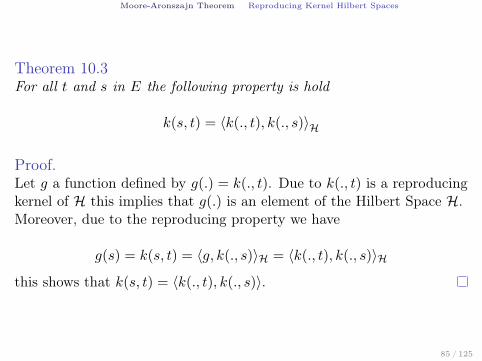
Theorem 10.3For all t and s in E the following property is hold
k(s, t) = 〈k(., t), k(., s)〉H
Proof.Let g a function defined by g(.) = k(., t). Due to k(., t) is a reproducingkernel of H this implies that g(.) is an element of the Hilbert Space H.Moreover, due to the reproducing property we have
g(s) = k(s, t) = 〈g, k(., s)〉H = 〈k(., t), k(., s)〉Hthis shows that k(s, t) = 〈k(., t), k(., s)〉.
85 / 125

Moore-Aronszajn Theorem Reproducing Kernel Hilbert Spaces
Examples of Reproducing Kernel Hilbert SpacesA Finite Dimensional Example
Theorem 10.4Let β = e1, e2, . . . , en an orthonormal basis of H and let define thefunction k as follows
k : E × E → C
(s, t) 7→ k(s, t) =
n∑i=1
ei(s)ei(t)
then k is a reproducing kernel.
86 / 125

Moore-Aronszajn Theorem Reproducing Kernel Hilbert Spaces
Proof.For all t in E, we have
k(., t) =
n∑i=1
ei(t)ei(.)
belongs to H (this is due to k(., t) is a linear combination of elements ofthe basis β). On the other hand, for all function ϕ of H we have
ϕ(.) =
n∑i=1
λiei(.)
then
87 / 125

Moore-Aronszajn Theorem Reproducing Kernel Hilbert Spaces
Proof.
〈ϕ, k(., t)〉H =
⟨n∑i=1
λiei(.),
n∑i=1
ei(t)ei(.)
⟩H
=
n∑i=1
λi
⟨ei(.),
n∑i=1
ei(t)ei(.)
⟩H
=
n∑i=1
n∑j=1
λiei(t) 〈ei, ej〉H︸ ︷︷ ︸=1
=
n∑i=1
λiei(t) = ϕ(t), ∀t ∈ E
88 / 125

Moore-Aronszajn Theorem Reproducing Kernel Hilbert Spaces
Corollary 10.5Every finite dimensional Hilbert Space H has a reproducing Kernel.
Proof.Let β = v1, . . . , vn a basis for the Hilbert Space H. Using theGram-Schmidt process on the set β we can build an orthonormal basisβ = v1, . . . , vn. Using the previous theorem we on this new basis βconclude that
k : E × E → C
(s, t) 7→ k(s, t) =n∑i=1
vi(s)vi(t)
is a Reproducing Kernel for H.
89 / 125

Moore-Aronszajn Theorem Reproducing Kernel Hilbert Spaces
For every t in E, we define the functional evalutation operator et of g inthe point t as the application
et : H → Cg 7→ et(g) = g(t)
b
bg(t) b
t
g
Figure: The functional evaluation et associated to any function g is the valueg(t) in the point t. 90 / 125

Moore-Aronszajn Theorem Reproducing Kernel Hilbert Spaces
Theorem 10.6A Hilbert spaces of complex function in E has a reproducing kernel ifand only if all the functional evaluations et, t in E, are continous in H.
91 / 125

Moore-Aronszajn Theorem Reproducing Kernel Hilbert Spaces
Corollary 10.7Let H an RKHS then all sequence which converges in norm convergepointwise to the same limit.
92 / 125

Moore-Aronszajn Theorem Reproducing Kernel Hilbert Spaces
Definition 10.8 (Semidefinite positive function)A function k : E × E → C is called semidefinite positive or positivetype function if
∀n ≥ 1, ∀(a1, . . . , an) ∈ Cn,∀(x1, . . . , xn) ∈ En,n∑i=1
n∑j=1
aiajk(xi, xj) ≥ 0(31)
93 / 125

Moore-Aronszajn Theorem Reproducing Kernel Hilbert Spaces
Lemma 10.9Let H a Hilbert Space with inner product 〈 ., 〉H (Not necesary anRKHS) and let ϕ : E → H, then, the function k defined as
k : E × E → C(x, y) 7→ k(x, y) = 〈ϕ(x), ϕ(y)〉H
is a semidefinite positive function.
94 / 125

Moore-Aronszajn Theorem Reproducing Kernel Hilbert Spaces
Lemma 10.10Every reproducing kernel is semidefinite positive.
95 / 125

Moore-Aronszajn Theorem Reproducing Kernel Hilbert Spaces
Lemma 10.11Let L a semdefinite positive function in E × E, then,1. For all x in E
L(x, x) ≥ 0
2. For all (x, y) in E × E holds
L(x, y) = L(y, x)
3. The function L is semidefinite positive.4. |L(x, y)|2 ≤ L(x, x)L(y, y).
96 / 125

Moore-Aronszajn Theorem Reproducing Kernel Hilbert Spaces
Lemma 10.12A real function L defined on E ×E is a semidefinite positive function ifand only if1. The L the function is symetric.2. ∀n ≥ 1,∀(a1, a2, . . . , an) ∈ Rn, ∀(x1, x2, . . . , xn) ∈ En,
n∑i=1
n∑j=1
aiajk(xi, xj) ≥ 0
97 / 125

Moore-Aronszajn Theorem Moore-Aronszajn Theorem
Definition 10.13 (pre-RKHS)A space which satifies the following properties.
1. Every the evaluation functionals et are continous in H0.2. Toda sucesión de Cauchy fn∞n=1 en H0 que converge
puntualmente a 0 también converge en norma a 0 en H0.
is called a pre-RKHS with reproducing kernel.
98 / 125

Moore-Aronszajn Theorem Moore-Aronszajn Theorem
Theorem 10.14Let H0 a subset of CE, the space of complex functions in E, with innerproduct 〈., .〉H0 and associated norm ‖.‖H0 then the hilbert space H withthe following properties
1. H0 ⊂ H ⊂ CE and the topology induced by 〈., .〉H0 en H0 concidewith the topology induced H0 by H.
2. H has a reproducing kernel k.
exists if and only if
1. All the functional evaluatins et are continous in H0.2. Every Cauchy sequence fn∞n=1 in H0 which converge pointwise to
0 converge to 0 in norm.
99 / 125

Moore-Aronszajn Theorem Moore-Aronszajn Theorem
H
H0
CE
Figure: H0 y H are subsets of the space of complex functions. H0 ⊂ H ⊂ CE
100 / 125

Moore-Aronszajn Theorem Moore-Aronszajn Theorem
Theorem 10.15 (Moore-Aronszajn Theorem)Let k a semidefinite positive function in E × E then exits a uniqueHilbert Space H of functions in E with reproducing kernel k such thatthe subspace H0 of H defined as
H0 = spank(., t) | t ∈ Eis dense in H and H is a set of functions in E which is the limit ofinner products of Cauchy sequences in H0.
101 / 125

References for Moore-Aronszajn Theorem
References for Moore-Aronszajn TheoremMain Sources:
[4] Alain Berlinet and Christine Thomas. Reproducing kernel Hilbertspaces in Probability and Statistics. Kluwer Academic Publishers,2004.
[42] D. Sejdinovic and A. Gretton. Foundations of Reproducing KernelHilbert Space I. url:http://www.stats.ox.ac.uk/~sejdinov/RKHS_Slides1.pdf(visited on 03/11/2012).
[43] D. Sejdinovic and A. Gretton. Foundations of Reproducing KernelHilbert Space II. url: http://www.gatsby.ucl.ac.uk/~gretton/coursefiles/RKHS_Slides2.pdf (visited on03/11/2012).
[44] D. Sejdinovic and A. Gretton. What is an RKHS? url:http://www.gatsby.ucl.ac.uk/~gretton/coursefiles/RKHS_Notes1.pdf (visited on 03/11/2012).
102 / 125

The kernel Trick

Kernel Trick Definitions
Definition 13.1 (Kernel)Let X a non-empty set. A function k : X ×X → K is called kernel inX if and only if there is Hilbert Space H and a mapping Φ : X → Hsuch that for all s, t it holds
k(t, s) := 〈Φ(t),Φ(s)〉H (32)
The function Φ is called feature mapping and H feature space of k.
104 / 125

Kernel Trick Definitions
Example 13.2Consider X = R and the function k defined by
k(s, t) = st =
⟨[s√2
s√2
],
[t√2t√2
]⟩
where the feature mappings are Φ(s) = s and Φ(s) =[s√2
s√2
]and the
features spaces are H = R and H = R2 respectly.
105 / 125

Kernel Trick Feature Space based on Mercer’s Theorem
Feature Space based on Mercer’s Theorem
The Mercer’s theorem allows to define a feature mapping for the kernelk as follows
k(t, s) =
∞∑j=1
λjϕj(t)ϕj(s)
=
⟨√λjϕj(t)
∞j=1
,√
λjϕj(s)∞j=1
⟩`2([a,b])
we can take `2([a, b]) as the feature space.
106 / 125

Kernel Trick Feature Space based on Mercer’s Theorem
Theorem 13.3The application Φ defined as
Φ : [a, b]→ `2([a, b])
t 7→√
λjϕj(t)∞j=1
es well defined and satifies
k(t, s) = 〈Φ(t),Φ(s)〉`2([a,b]) (33)
107 / 125

Kernel Trick Feature Space based on Mercer’s Theorem
Theorem 13.4 (Mercer Representation of RKHS)Let X a compact metric space and k : X ×X → R a continous kernel.We defined the set H as
H =
f ∈ L2(X)
∣∣∣∣ f =
∞∑j=1
ajϕj where
aj√λj
∞j=1
∈ `2 (34)
with inner product ⟨ ∞∑j=1
ajϕj ,
∞∑j=1
bjϕj
⟩H
=
∞∑j=1
ajbjλj
(35)
then H is a RKHS with reproducing kernel k.
108 / 125

History

History
Timeline
Table: Timeline of Support Vector Machines Algorithm Development
1909 • Mercer Theorem — James Mercer."Functions of Positive and Negative Type, and their Connection with the
Theory of Integral Equations".
1950 • "Moore-Aronzajn Theorem" — Nachman Aronszajn."Reproducing Kernel Hilbert Spaces".
1964 • Introduced the geometrical interpretation of the kernels asinner products in a feature space — Aizerman, Bravermanand Rozonoer."Theoretical Foundations of the Potential Function Method in Pattern
Recognition Learning".
1964 • Original SVM algorithm — Vladimir Vapnik and AlexeyChervonenkis."A Note on One Class of Perceptrons"
110 / 125

History
Timeline
Table: Timeline of Support Vector Machines Algorithm Development
1965 • Cover’s Theorem — Thomas Cover."Geometrical and Statistical Properties of Systems of Linear Inequalities
with Applications in Pattern Recognition".
1992 • Support Vector Machines — Bernhard Boser, IsabelleGuyon and Vladimir Vapnik."A Training Algorithm for Optimal Margin Classifiers".
1995 • Soft Support Vector Machines — Corinna Cortes andVladimir Vapnik."Support Vector Networks".
111 / 125

References

References
References I
[1] Yaser S. Abu-Mostafa, Malik Magdon-Ismail, andHsuan-Tien Lin. Learning From Data: A short course. AMLBook, 2012.
[2] Nachman Aronszajn. “Theory of Reproducing Kernels”. In:Transactions of the American Mathematical Society 68 (1950),pp. 337–404.
[3] C. Berg, J. Reus, and P. Ressel. Harmonic Analysis onSemigroups: Theory of Positive Definite and Related Functions.Springer Science+Business Media, LLV, 1984.
[4] Alain Berlinet and Christine Thomas. Reproducing kernel Hilbertspaces in Probability and Statistics. Kluwer Academic Publishers,2004.
[5] Donald L. Cohn. Measure Theory. Birkhäuser, 2013.
113 / 125

References
References II
[6] Corinna Cortes and Vladimir Vapnik. “Support Vector Networks”.In: Machine Learning (1995), pp. 273–297.
[7] Thomas Cover. “Geometrical and Statistical properties of systemsof linear inequalities with applications in pattern recognition”. In:IEEE Transactions on Electronic Computer (), pp. 326–334.
[8] Nello Cristianini and John Shawe-Taylor. An Introduction toSupport Vector Machines and Other Kernel-based LearningMethods. Cambridge University Press, 2000.
[9] Felipe Cucker and Ding Xuan Zhou. Learning Theory.Cambridge University Press, 2007.
[10] Steve Cucker Felipe; Smale. “On the Mathematical Foundationsof Learning”. In: Bulletin of the American Mathematical Society(), pp. 1–49.
114 / 125

References
References III
[11] Naiyang Deng, Yingjie Tian, and Chunhua Zhang. Support VectorMachines: Optimization Based Theory, Algorithms, andExtensions. CRC Press, 2013.
[12] Ke-Lin Du and M. N. S. Swamy. Neural Networks and StatisticalLearning. Springer Science & Business Media, 2013.
[13] Nelson Dunford and Jacob T. Schwartz. Linear Opertors Part II:Spectral Theory Self Adjoint Operators in Hilbert Space.Interscience Publishers, 1963.
[14] Lawrence C. Evans. Partial Differential Equations. AmericanMathematical Society, 1998.
[15] Gregory Fasshauer. Positive Definite Kernels: Past, Present andFuture. url: http://www.math.iit.edu/~fass/PDKernels.pdf.
115 / 125

References
References IV
[16] Gregory E. Fasshauer. Positive Definite Kernels: Past, Presentand Future. url:http://www.math.iit.edu/~fass/PDKernels.pdf.
[17] Israel Gohberg, Seymour Goldberg, and Marinus A. Kaashoek.Basic Classes of Linear Operators. Birkhäuser, 2003.
[18] Lutz Hamel. Knowledge Discovery with Support Vector Machines.Wiley-Interscience, 2009.
[19] Simon Haykin. Neural Networks and Learning Machines. ThirdEdition. Pearson Prentice Hall, 2009.
[20] Operadores integrais positivos e espaços de Hilbert de reprodução.“José Claudinei Ferreira”. PhD thesis. USP - São Carlos, 2010.
116 / 125

References
References V
[21] David Hilbert. “Grundzüge einer allgeminen Theorie der linarenIntegralrechnungen.” In: Nachrichten, Math.-Phys. Kl (1904),pp. 49–91. url: http://www.digizeitschriften.de/dms/img/?PPN=GDZPPN002499967.
[22] Harry Hochstadt. Integral Equations. Wiley, 1989.
[23] Alexey Izmailov and Mikhail Solodov. Otimização Vol.1Condições de Otimalidade, Elementos de Analise Convexa e deDualidade. Third Edition. IMPA, 2014.
[24] Thorsten Joachims. Learning to Classify Text Using SupportVector Machines: Methods, Theory and Algorithms. KluwerAcademic Publishers, 2002.
[25] J. Zico Kolter. MLSS 2014 – Introduction to Machine Learning.url: http://www.mlss2014.com/files/kolter_slides1.pdf.
117 / 125

References
References VI
[26] Hermann König. Eigenvalue Distribution of Compact Operators.Birkhäuser, 1986.
[27] Elon Lages. Analisis Real, Volumen 1. Textos del IMCA, 1997.
[28] Peter D. Lax. Functional Analysis. Wiley, 2002.
[29] Le, Sarlos, and Smola. “Fastfood - Approximating KernelExpansions in Loglinear Time”. In: ICML 2013 ().
[30] James Mercer. “Functions of positive and negative type and theirconnection with the theory of integral equations”. In:Philosophical Transactions of the Royal Society (1909),pp. 415–446.
[31] Mehryar Mohri, Afshin Rostamizadeh, and Ameet Talwalkar.Foundations of Machine Learning. The MIT Press, 2012.
118 / 125
References
References VII[32] F. Pedregosa et al. “Scikit-learn: Machine Learning in Python”.
In: Journal of Machine Learning Research 12 (2011),pp. 2825–2830.
[33] Anthony L. Peressini, Francis E. Sullivan, and J.J. Jr. Uhl. TheMathematics of Nonlinear Programming. Springer, 1993.
[34] David Porter and David S. G. Stirling. Integral Equations: Apractical treatment, from spectral theory to applications.Cambridge University Press, 1990.
[35] Carl Edward Rasmussen and Christopher K. I. Williams.Gaussian Processes for Machine Learning. The MIT Press, 2006.
[36] Frigyes Riesz and Béla Sz.-Nagy. Functional Analysis. DoverPublications, Inc, 1990.
[37] Walter Rudin. Principles of Mathematical Analysis.McGraw-Hill, Inc., 1964.
119 / 125

References
References VIII
[38] Saburou Saitoh. Theory of reproducing kernels and itsappplications. Longman Scientific & Technical, 1988.
[39] Bernhard Schlköpf and Alexander Smola. Learning with Kernels:Support Vector Machines, Regularization, Optimization, andBeyond. The MIT Press, 2001.
[40] E. Schmidt. “Über die Auflösung linearer Gleichungen mitUnendlich vielen unbekannten”. In: Rendiconti del CircoloMatematico di Palermo (1908), pp. 53–77. url:http://link.springer.com/article/10.1007/BF03029116.
[41] Bernhard Schölkopf. What is Machine Learning? MachineLearning Summer School 2013 Tübingen, 2013.
120 / 125

References
References IX
[42] D. Sejdinovic and A. Gretton. Foundations of Reproducing KernelHilbert Space I. url:http://www.stats.ox.ac.uk/~sejdinov/RKHS_Slides1.pdf(visited on 03/11/2012).
[43] D. Sejdinovic and A. Gretton. Foundations of Reproducing KernelHilbert Space II. url: http://www.gatsby.ucl.ac.uk/~gretton/coursefiles/RKHS_Slides2.pdf (visited on03/11/2012).
[44] D. Sejdinovic and A. Gretton. What is an RKHS? url:http://www.gatsby.ucl.ac.uk/~gretton/coursefiles/RKHS_Notes1.pdf (visited on 03/11/2012).
[45] Alex Smola. 4.2.2 Kernels - Machine Learning Class 10-701.url: https://www.youtube.com/watch?v=0Nis-oMLbDs.
121 / 125

References
References X
[46] Alexander Stantnikov et al. A Gentle Introduction to SupportVector Machines in Biomedicine. World Scientific, 2011.
[47] Ingo Steinwart and Christmannm Andreas. Support VectorMachines. 2008.
[48] Yichuan Tang. Deep Learning using Linear Support VectorMachines. url: http://deeplearning.net/wp-content/uploads/2013/03/dlsvm.pdf.
[49] Sergios Theodoridis. Machine Learning: A Bayesian andOptimization Perspective. Academic Press, 2015.
[50] Joachims Thorsten. Learning to Classify Text Using SupportVector Machines. Springer, 2002.
[51] Vladimir Vapnik. Estimation of Dependences Based on EmpiricalData. Springer, 2006.
122 / 125

References
References XI
[52] Grace Wahba. Spline Models for Observational Data. SIAM,1900.
[53] Holger Wendland. Scattered Data Approximation. CambridgeUniversity Press, 2005.
[54] Eberhard Zeidler. Applied Functional Analysis: Main Principlesand Their Applications. Springer, 1995.
[55] Stephen M. Zemyan. The Classical Theory of Integral Equations:A Concise Treatment. Birkhauser, 2010.
123 / 125

Questions?

Thanks