The Kazhdan-Lusztig polynomial of a matroid

Ben Elias

Department of Mathematics, University of Oregon, Eugene, OR 97403

belias@uoregon.edu

Nicholas Proudfoot1

Department of Mathematics, University of Oregon, Eugene, OR 97403

njp@uoregon.edu

Max Wakefield2

Department of Mathematics, United States Naval Academy, Annapolis, MD 21402

wakefiel@usna.edu

Abstract. We associate to every matroid M a polynomial with integer coefficients, which we

call the Kazhdan-Lusztig polynomial of M , in analogy with Kazhdan-Lusztig polynomials in

representation theory. We conjecture that the coefficients are always non-negative, and we

prove this conjecture for representable matroids by interpreting our polynomials as intersection

cohomology Poincare polynomials. We also introduce a q-deformation of the Mobius algebra

of M , and use our polynomials to define a special basis for this deformation, analogous to

the canonical basis of the Hecke algebra. We conjecture that the structure coefficients for

multiplication in this special basis are non-negative, and we verify this conjecture in numerous

examples.

1 Introduction

Our goal is to develop Kazhdan-Lusztig theory for matroids in analogy with the well-known theory

for Coxeter groups. In order to make this analogy clear, we begin by summarizing the most relevant

features of the usual theory.

Given a Coxeter group W along with a pair of elements y, w ∈W , Kazhdan and Lusztig [KL79]

associated a polynomial Px,y(t) ∈ Z[t], which is non-zero if and only if x ≤ y in the Bruhat order.

This polynomial has a number of different interpretations:

• Combinatorics: There is a purely combinatorial recursive definition of Px,y(t) in terms of

more elementary polynomials, called R-polynomials. See [Lus83, Proposition 2], as well as

[BB05, §5.5] for a more recent account.

• Geometry: If W is a finite Weyl group, then Px,y(t) may be interpreted as the Poincare

polynomial of a stalk of the intersection cohomology sheaf on a Schubert variety in the

associated flag variety [KL80]. The Schubert variety is determined by y, and the point at

1Supported by NSF grant DMS-0950383.2Supported by the Simons Foundation and the Office of Naval Research.

1

which one takes the stalk is determined by x. This proves that Px,y(t) has non-negative

coefficients when W is a finite Weyl group. The non-negativity of the coefficients of Px,y(t)

for arbitrary Coxeter groups was conjectured in [KL79], but was only recently proved by

Williamson and the first author [EW14, 1.2(1)].

• Algebra: The polynomials Px,y(t) are the entries of the matrix relating the Kazhdan-Lusztig

basis (or canonical basis) to the standard basis of the Hecke algebra of W , a q-deformation

of the group algebra C[W ]. When W is a finite Weyl group, Kazhdan and Lusztig showed

that the structure coefficients for multiplication in the Kazhdan-Lusztig basis are polynomials

with non-negative coefficients. For general Coxeter groups, this is proved in [EW14, 1.2(2)].

In our analogy, the Coxeter group W is replaced by a matroid M , and the elements x, y ∈ Ware replaced by flats F and G of M . We only define a single polynomial PM (t) for each matroid,

but one may associate to a pair F ≤ G the polynomial PMFG

(t), where MFG is the matroid whose

lattice of flats is isomorphic to the interval3 [F,G]. The role of the R-polynomial is played by the

characteristic polynomial of the matroid. The analogue of being a finite Weyl group is being a

representable matroid; that is, the matroid MA associated to a collection A of vectors in a vector

space. The analogue of a Schubert variety is the reciprocal plane XA, also known as the spectrum

of the Orlik-Terao algebra of A. The analogue of the group algebra C[W ] is the Mobius algebra

E(M); we introduce a q-defomation Eq(M) of this algebra which plays the role of the Hecke algebra.

All of these analogies may be summarized as follows:

• Combinatorics: We give a recursive definition of the polynomial PM (t) in terms of the

characteristic polynomial of a matroid (Theorem 2.2), and we conjecture that the coefficients

are non-negative (Conjecture 2.3).

• Geometry: If M is representable over a finite field, we show that PM (t) is equal to the `-adic

etale intersection cohomology Poincare polynomial of the reciprocal plane4 (Theorem 3.10).

Any matroid that is representable over some field is representable over a finite field, thus we

obtain a proof of Conjecture 2.3 for all representable matroids (Corollary 3.11).

• Algebra: We use the polynomials PMFG

(t) to define the Kazhdan-Lusztig basis of the q-

deformed Mobius algebra Eq(M). We conjecture that the structure constants for multiplica-

tion in this basis are polynomials in q with non-negative coefficients (Conjecture 4.2), and we

verify this conjecture in a number of cases.

Remark 1.1. Despite these parallels, the behavior of the polynomials for matroids differs drasti-

cally from the behavior of ordinary Kazhdan-Lusztig polynomials for Coxeter groups. In particular,

3We note that this shortcut has no analogue in ordinary Kazhdan-Lusztig theory, since the interval [x, y] is notin general isomorphic to the Bruhat poset of some other Coxeter group. Furthermore, it is still an open questionwhether or not Px,y(t) is determined by the isomorphism type of the interval [x, y].

4The reciprocal plane is a cone, so we could equivalently say that it is the Poincare polynomial of the stalk of theintersection cohomology sheaf at the cone point.

2

one does not recover the classical Kazhdan-Lusztig polynomials for the Coxeter group Sn from the

braid matroid. Polo [Pol99] has shown that any polynomial with non-negative coefficients and

constant term 1 appears as a Kazhdan-Lusztig polynomial associated to some symmetric group,

while Kazhdan-Lusztig polynomials of matroids are far more restrictive (see Proposition 2.14).

The original work of Kazhdan and Lusztig begins with an algebraic question (How can we

find a basis for the Hecke algebra with certain nice properties?), which led them to both the

combinatorics and the geometry. In our work, we began with a geometric question (What is the

intersection cohomology of the reciprocal plane?), which led us naturally to the combinatorics. The

algebraic facet of our work is somewhat more speculative and ad hoc, representing an attempt to

trace backward the route of Kazhdan and Lusztig.

There is no known convolution product in the geometry of the reciprocal plane which would

account for the q-deformed Mobius algebra Eq(M), as the convolution product on flag varieties

produces the Hecke algebra. Unlike in the Coxeter setting, the Kazhdan-Lusztig basis of Eq(M)

currently has no intrinsic definition, and the theory of this basis is far less satisfactory. For example,

the basis is cellular, but in a trivial way: the cells are all one-dimensional. The identity is not an

element of the basis.

Remark 1.2. When W is a finite Weyl group, yet another important interpretation of Px,y(t) is

that it records the multiplicity space of a simple module in a Verma module in the graded lift

of Berstein-Gelfand-Gelfand category O [BB81, BK81]. The analogous goal for matroids would

be a categorification of the q-deformed Mobius algebra Eq(M), or its regular representation. The

Mobius algebra E(M) is categorified by a monoidal category of “commuting” quiver representations

[Bac79, Theorem 7], but we do not know how to modify this category to produce a categorification

of Eq(M).

Having made these caveats, the observed phenomenon of positivity indicates that our Kazhdan-

Lusztig basis does hold interest. There are numerous other ways one could have used the Kazhdan-

Lusztig polynomials of a matroid as a change of basis matrix, but the corresponding bases do not

have positive structure coefficients. As seen in Remark 4.8, positivity is a subtle question, and

would fail if all the Kazhdan-Lusztig polynomials were trivial.

We now give a more detailed summary of the contents of the paper. Section 2 (Combinatorics)

is dedicated to the combinatorial definition of PM (t) along with basic properties and examples.

In addition to our conjecture that the coefficients of PM (t) are non-negative (Conjecture 2.3), we

also conjecture that they form a log concave sequence (Conjecture 2.5). We explicitly compute the

coefficients of t and t2 in terms of the Whitney numbers of the lattice of flats of M (Propositions

2.12 and 2.16). We prove non-negativity of the linear coefficient (Proposition 2.14), and we give

formulas for the quadratic and cubic term (Propositions 2.16 and 2.18), though even in these

cases we cannot prove non-negativity (Remark 2.17). We prove a product formula for direct sums

(Proposition 2.7), which eliminates the possibility of “cheap” counterexamples to Conjecture 2.3

(Remark 2.8).

3

We also study in detail the cases of uniform matroids and braid matroids. For uniform matroids,

we provide an even more explicit computation of the polynomial up to the cubic term (Corollary

2.20). For the braid matroid Mn corresponding to the complete graph on n vertices, we explain

how to compute the coefficients of the Kazhdan-Lusztig polynomial using Stirling numbers. In

an appendix, written jointly with Ben Young, we give tables of Kazhdan-Lusztig polynomials of

uniform matroids and braid matroids of low rank. The polynomials that we see are unfamiliar; in

particular, they do not appear to be related to any known matroid invariants. For both uniform

matroids and braid matroids, we express the defining recursion in terms of a generating function

identity (Propositions 2.21 and 2.27).

The purpose of Section 3 (Geometry) is to prove that, if MA is the matroid associated to a

vector arrangement A over a finite field, then the Kazhdan-Lusztig polynomial of MA coincides with

the `-adic etale intersection cohomology Poincare polynomial of the reciprocal plane XA (Theorem

3.10). The key ingredient to our proof is Theorem 3.3, which says that, in an etale neighborhood

of any point, XA looks like the product of a vector space with a neighborhood of the cone point in

the reciprocal plane of a certain smaller hyperplane arrangement. This improves upon a result of

Sanyal, Sturmfels, and Vinzant [SSV13, Theorem 24], who prove the analogous statement on the

level of tangent cones.

We conclude Section 3 with a digression in which we discuss a certain question of Li and Yong

[LY11]. Given a point on a variety, they compare two polynomials: the local intersection coho-

mology Poincare polynomial, and the numerator of the Hilbert series of the tangent cone. They

are interested in the case of Schubert varieties, where the first polynomial is a Kazhdan-Lusztig

polynomial. We consider the case of reciprocal planes, where the first polynomial is the Kazhdan-

Lusztig polynomial of a matroid and the second polynomial is the h-polynomial of the broken

circuit complex of the same matroid.

Section 4 (Algebra) deals with the Mobius algebra of a matroid, which has a Z-basis given by

flats with multiplication given by the join5 operation: εF ·εG = εF∨G. We introduce a q-deformation

of this algebra; that is, a commutative, associative, unital Z[q, q−1]-algebra with basis given by flats,

such that specializing q to 1 recovers the original Mobius algebra (Proposition 4.1). Using Kazhdan-

Lusztig polynomials, we define a new basis whose relationship to the standard basis is analogous

to the relationship between the canonical basis and standard basis for the Hecke algebra, and we

conjecture that the structure coefficients for multiplication in the new basis lie in N[q] (Conjecture

4.2). We verify this conjecture for Boolean matroids (Proposition 4.5), for uniform matroids of

rank at most 3 (Subsection 4.4), and for braid matroids of rank at most 3 (Subsection 4.5).

5In the literature, one usually sees the multiplication given by meet rather than join. However, these two productsare isomorphic; indeed, both are isomorphic to the coordinatewise product [Sol67]. The join product will be morenatural for our purposes.

4

Addendum: After this paper was published, Ben Young discovered counterexamples to Conjecture

4.2. See Section 4.6.

Acknowledgments: The authors would like to thank June Huh, Joseph Kung, Emmanuel Letellier,

Carl Mautner, Hal Schenck, Ben Webster, Ben Young, and Thomas Zaslavsky for their helpful

contributions. The third author is grateful to the University of Oregon for its hospitality during

the completion of this project.

2 Combinatorics

In this section we give a combinatorial definition of the Kazhdan-Lusztig polynomial of a matroid,

we compute the first few coefficients, and we study the special cases of uniform matroids and braid

matroids.

2.1 Definition

Let M be a matroid with no loops on a finite ground set I. Let L(M) ⊂ 2I denote the lattice of

flats of M , ordered by inclusion, with minimum element ∅. Let µ be the Mobius function on L(M),

and let

χM (t) =∑

F∈L(M)

µ(∅, F ) trkM−rkF

be the characteristic polynomial of M . For any flat F ∈ L(M), let IF = IrF and IF = F . Let

MF be the matroid on IF consisting of subsets of IF whose union with a basis for F are independent

in M , and let MF be the matroid on IF consisting of subsets of IF which are independent in M .

We call the matroid MF the restriction of M at F , and MF the localization of M at F .

(This terminology and notation comes from the corresponding constructions for arrangements; see

Subsection 3.1.) We have rkMF = rkM − rkF and rkMF = rkF .

Lemma 2.1. For any matroid M of positive rank,∑

F∈L(M)

trkFχMF(t−1)χMF (t) = 0.

Proof. We have∑F

trkFχMF(t−1)χMF (t) =

∑F

trkF∑E≤F

µ(∅, E) trkE−rkF∑G≥F

µ(F,G) trkM−rkG

=∑

E≤F≤Gµ(∅, E)µ(F,G) trkM+rkE−rkG

= trkM∑E≤G

µ(∅, E) trkE−rkG∑

F∈[E,G]

µ(F,G).

5

The internal sum is equal to δ(E,G) [OT92, 2.38], thus our equation simplifies to∑F

trkFχMF(t−1)χMF (t) = trkM

∑F

µ(∅, F ).

This is 0 unless rkM = 0.

The following is our first main result.

Theorem 2.2. There is a unique way to assign to each matroid M a polynomial PM (t) ∈ Z[t] such

that the following conditions are satisfied:

1. If rkM = 0, then PM (t) = 1.

2. If rkM > 0, then degPM (t) < 12 rkM .

3. For every M , trkMPM (t−1) =∑F

χMF(t)PMF (t).

The polynomial PM (t) will be called the Kazhdan-Lusztig polynomial of M . Our proof of

Theorem 2.2 closely follows Lusztig’s combinatorial proof of the existence of the usual Kazhdan-

Lusztig polynomials [Lus83, Proposition 2], which he attributes to Gabber.

Proof. Let M be a matroid of positive rank. We may assume inductively that PM ′(t) has been

defined for every matroid M ′ of rank strictly smaller than rkM ; in particular, PMF (t) has been

defined for all ∅ 6= F ∈ L(M). Let

RM (t) :=∑∅6=F

χMF(t)PMF (t);

then item 3 says exactly that

trkMPM (t−1)− PM (t) = RM (t).

It is clear that there can be at most one polynomial PM (t) of degree strictly less than 12 rkM

satisfying this condition. The existence of such a polynomial is equivalent to the statement

trkMRM (t−1) = −RM (t).

6

We have

trkMRM (t−1) = trkM∑∅6=F

χMF(t−1)PMF (t−1)

=∑∅6=F

trkFχMF(t−1)trkM

FPMF (t−1)

=∑∅6=F≤G

trkFχMF(t−1)χMF

G(t)PMG(t)

=∑∅6=G

−χMG(t)PMG(t) + PMG(t)

∑F≤G

trkFχMF(t−1)χMF

G(t)

.

Since rkMG = rkG 6= 0, Lemma 2.1 says that the internal sum is zero for all G 6= ∅, so our equation

simplifies to trkMRM (t−1) = −∑∅6=G

χMG(t)PMG(t) = −RM (t).

Conjecture 2.3. For any matroid M , the coefficients of the Kazhdan-Lusztig polynomial PM (t)

are non-negative.

Remark 2.4. In Section 3, we will prove Conjecture 2.3 for representable matroids by providing

a cohomological interpretation of the polynomial PM (t) (Theorem 3.10).

Based on our computer computations for uniform matroids and braid matroids (see appendix),

along with Proposition 2.14 and Remark 2.15, we make the following additional conjecture. A

sequence e0, . . . , er is called log concave if, for all 1 < i < r, ei−1ei+1 ≤ e2i . It is said to have

no internal zeros if the set {i | ei 6= 0} is an interval. Note that a log concave sequence of

non-negative integers with no internal zeroes is always unimodal.

Conjecture 2.5. For any matroid M , the coefficients of PM (t) form a log concave sequence with

no internal zeroes.

Remark 2.6. If M is representable, then Huh and Katz proved that the absolute values of the

coefficients of χM (q) form a log concave sequence with no internal zeroes [HK12, 6.2], solving a

conjure of Read for graphical matroids and the representable case of a conjecture of Rota-Heron-

Walsh for arbitrary matroids.

2.2 Direct sums

The following proposition says that the Kazhdan-Lusztig polynomial is multiplicative on direct

sums.

Proposition 2.7. For any matroids M1 and M2, PM1⊕M2(t) = PM1(t)PM2(t).

7

Proof. We proceed by induction. The statement is clear when rkM1 = 0 or rkM2 = 0. Now

assume that the statement holds for M ′1 and M ′2 whenever rkM ′1 ≤ rkM1 and rkM ′2 ≤M2 with at

least one of the two inequalities being strict.

We have L(M1⊕M2) = L(M1)×L(M2). The localization of M1⊕M2 at (F1, F2) is isomorphic to

(M1)F1⊕(M2)F2 , and the restriction at (F1, F2) is isomorphic to (M1)F1⊕(M2)F2 . The characteristic

polynomial of (M1)F1 ⊕ (M2)F2 is the product of the two characteristic polynomials, and our

inductive hypothesis tells us that the Kazhdan-Lusztig polynomial of (M1)F1⊕(M2)F2 is the product

of the two Kazhdan-Lusztig polynomials, provided that F1 6= ∅ or F2 6= ∅. These two observations,

along with the recursive definition of the Kazhdan-Lusztig polynomial, combine to tell us that

trkM1+rkM2PM1⊕M2(t−1)− trkM1PM1(t−1) · trkM2PM2(t−1) = −PM1(t)PM2(t) + PM1⊕M2(t).

The left-hand side is concentrated in degree strictly greater than 12 rkM1 + 1

2 rkM2, while the right-

hand side is concentrated in degree strictly less than 12 rkM1 + 1

2 rkM2. This tells us that both

sides must vanish, and the proposition is proved.

Remark 2.8. Proposition 2.7 rules out many potential counterexamples to Conjecture 2.3. That

is, one cheap way to construct a non-representable matroid is to fix a prime p and let M = M1⊕M2,

where M1 is representable only in characteristic p and M2 is representable only in characteristic 6= p.

Proposition 2.7 will tells that the Kazhdan-Lusztig polynomial of M1⊕M2 is equal to the product

of the Kazhdan-Lusztig polynomials of M1 and M2, each of which has non-negative coefficients

because M1 and M2 are both representable.

Remark 2.9. Proposition 2.7 is also consistent with Conjecture 2.5, since the convolution of two

non-negative log concave sequences with no internal zeroes is again log concave with no internal

zeroes [Koo06, Theorem 1]. Note that the corresponding statement would be false without the no

internal zeroes hypothesis.6

Corollary 2.10. If M is the Boolean matroid on any finite set, then PM (t) = 1.

Proof. The Boolean matroid on a set of cardinality n is isomorphic to the direct sum of n copies

of the unique rank 1 matroid on a set of cardinality 1.

2.3 The first few coefficients

In this subsection we interpret the first few coefficients of PM (t) in terms of the doubly indexed

Whitney numbers of M , introduced by Green and Zaslavsky [GZ83].

Proposition 2.11. The constant term of PM (t) is equal to 1.

6We thank June Huh for pointing out this fact.

8

Proof. We proceed by induction on the rank of M . If rkM = 0, then PM (t) = 1 by definition. If

rkM > 0, we consider the recursion

trkMPM (t−1) =∑F

χMF(t)PMF (t).

Since degPM (t) < rkM , the left-hand side has no constant term, therefore we have

0 =∑F

χMF(0)PMF (0).

By our inductive hypothesis, we may assume that PMF (0) = 1 for all nonempty flats F , and we

therefore need to show that

0 =∑F

χMF(0).

This follows from the fact that χMF(0) = µ(∅, F ) and rkM > 0.

For all natural numbers i and j, let

wi,j :=∑

rkE=i,rkF=j

µ(E,F ) and Wi,j :=∑

rkE=i,rkF=j

ζ(E,F ),

where ζ(E,F ) = 1 if E ≤ F and 0 otherwise. These are called doubly indexed Whitney

numbers of the first and second kind, respectively. In the various propositions that follow, we let

d = rkM .

Proposition 2.12. The coefficient of t in PM (t) is equal to W0,d−1 −W0,1.

Proof. We consider the defining recursion

trkMPM (t−1) =∑F

χMF(t)PMF (t)

and compute the coefficient of trkM−1 on the right-hand side. The flat F = I contributes −W0,1,

and each of the W0,d−1 flats of rank d− 1 contributes 1.

Remark 2.13. If M is the matroid associated to a hyperplane arrangement, Proposition 2.12 says

that the coefficient of t in PM (t) is equal to the number of lines in the lattice of flats minus the

number of hyperplanes.

Proposition 2.14. The coefficient of t in PM (t) is always non-negative, and the following are

equivalent:

(i) PM (t) = 1

(ii) the coefficient of t is zero

(iii) the lattice L(M) is modular.

9

Proof. Non-negativity of the linear term follows from Proposition 2.12 along with the hyperplane

theorem [Aig87, 8.5.1 & §8.5]. The hyperplane theorem also states that the linear term is zero if

and only if L(M) is modular. The first item obviously implies the second, so it remains only to

show that PM (t) = 1 whenever L(M) is modular.

We proceed by induction on d = rkM . The base case is trivial. Assume the statement holds

for all matroids of rank smaller than d, and that L(M) is modular. In particular, for any flat F ,

L(MF ) is also modular, so we may assume that PMF (t) = 1 for all F 6= ∅. Thus the defining

recursion says that

tdPM (t−1)− PM (t) =∑F 6=∅

χMF(t),

and we need only show that the right-hand side is equal to td − 1. Equivalently, we need to show

that∑

F χMF(t) is equal to td.

Since L(M) is modular, there exists another matroid M ′ such that L(M ′) is dual to L(M); that

is, there exists an order-reversing and rank-reversing bijection between L(M) and L(M ′). (This

is simply the statement that the dual of L(M) is again a geometric lattice, which follows from

modularity.) This implies that∑F

χMF(t) =

∑F,G

µM (F,G)td−rkM G =∑F,G

µM ′(G,F )trkM′ G.

By Mobius inversion, this sum vanishes in all degrees less than d, and the coefficient of td is equal

to µM ′(I, I) = 1.

Remark 2.15. Note that the implication of (i) by (ii) in Proposition 2.14 provides evidence for

the lack of internal zeroes in the sequence of coefficients of PM (t) (Conjecture 2.5).

Proposition 2.16. The coefficient of t2 in PM (t) is equal to

w0,2 −W1,d−1 +W0,d−2 −Wd−3,d−2 +Wd−3,d−1.

Proof. We again consider the defining recursion, and this time we compute the coefficient of trkM−2

on the right-hand side. The flat F = I contributes w0,2, each flat F of rank d − 1 contributes

−W0,1(MF ), and −∑

rkF=d−1W0,1(MF ) = −W1,d−1. Each of the W0,d−2 flats of rank d − 2

contributes 1. Each flat F of rank d − 3 contributes the linear term of PMF (t), which is equal

to W0,2(MF ) −W0,1(MF ) by Proposition 2.12. Summing over all such flats, we obtain the final

two terms Wd−3,d−1 −Wd−3,d−2.

Remark 2.17. We have w0,2 = W1,2 −W0,2,

W1,2 −W1,d−1 =∑

rkF=1

(W0,1(MF )−W0,d−2(MF )

),

10

and

Wd−3,d−1 −Wd−3,d−2 =∑

rkG=d−3

(W0,2(MG)−W0,1(MG)

),

thus the coefficient of t2 is equal to∑rkF=1

(W0,1(MF )−W0,d−2(MF )

)+

∑rkG=d−3

(W0,2(MG)−W0,1(MG)

)+(W0,d−2 −W0,2

).

The hyperplane theorem says that each of the summands in the first sum is non-positive and each of

the summands in the second sum is non-negative. The statement that W0,d−2−W0,2 is non-negative

as long as d ≥ 4 is a long standing conjecture in matroid theory, called the “top-heavy conjecture”

[DW75], [Kun86, 2.5.2]. (Note that if d ≤ 4, then the coefficient of t2 in PM (t) is automatically

zero.) Thus a comparison (in either direction) between the absolute values of the two sums would

yield a logical implication (in the corresponding direction) between Conjecture 2.3 (for quadratic

terms) and the top-heavy conjecture.

The next proposition, whose proof we omit, indicates the difficulty with finding a closed formula

for these coefficients. On the other hand, [Wak, 5.5] presents a formula for all coefficients, albeit

recursively defined, in the same vein as Proposition 2.16.

Proposition 2.18. The coefficient of t3 in PM (t) is equal to

w0,3 −Wd−4,d−3 +Wd−4,d−1 −W1,d−2 +W0,d−3

+∑

rkF=d−1

w0,2(MF )−∑

rkF=d−3

W0,1(MF )[W0,2(MF )−W0,1(MF )

]+

∑rkF=d−5

[w0,2(MF )−W1,4(MF ) +W0,3(MF ) +W2,4(MF )−W2,3(MF )

].

2.4 Uniform matroids

Given non-negative integers d and m, let Mm,d be the uniform matroid of rank d on a set of

cardinality m+ d, and write

PMm,d(t) = Pm,d(t) =

∑i

cim,d ti.

The values of Pm,d(t) for small m and d appear in the appendix.

For any flat F of rank strictly less than d, the localization (Mm,d)F is a Boolean matroid, and

the restriction MFm,d is isomorphic to Mm,d−rkF , thus our recursive definition will give us a recursive

relation among the coefficients cim,d for a single fixed m. Specifically, we have the following result

(the factor before cjm,k is a trinomial coefficient).

11

Proposition 2.19. For any m, d, and i, we have

cim,d = (−1)i(m+ d

i

)+

i−1∑j=0

i+j∑k=2j+1

(−1)i+j+k(

m+ d

m+ k, i+ j − k, d− i− j

)cjm,k.

We can use Proposition 2.19 obtain explicit formulas for the first few coefficients. In general,

the formula for cim,d will be a signed sum of (i+ 1)-nomial coefficients, each with m+ d on top. We

omit the proof of Corollary 2.20 because it is a straightforward application of the proposition.

Corollary 2.20. We have

c0m,d = 1

c1m,d =

(m+dm+1

)−(m+d

1

)c2m,d =

(m+d

m+1,d−3,2

)−(

m+dm+1,d−2,1

)+(

m+dm+2,d−2,0

)−(

m+dm+2,d−3,1

)+(m+d

2

)c3m,d =

(m+d

m+1,d−3,2,0

)−(

m+dm+1,d−4,2,1

)+(

m+dm+1,d−4,3,0

)−(

m+dm+1,d−5,3,1

)+(

m+dm+1,d−5,2,2

)−(

m+dm+2,d−3,1,0

)+(

m+dm+2,d−4,1,1

)−(

m+dm+2,d−5,2,1

)+(

m+dm+2,d−5,3,0

)+(

m+dm+3,d−3,0,0

)−(

m+dm+3,d−4,1,0

)+(

m+dm+3,d−5,2,0

)−(m+d

3

).

We can also express our recursion in terms of a generating function identity. Let

Φm(t, u) =

∞∑d=1

Pm,d(t)ud.

Proposition 2.21. We have

Φm(t−1, tu) =tu− u

(1− tu+ u)(1 + u)m+

1

(1− tu+ u)m+1Φm

(t,

u

1− tu+ u

).

Proof. Our defining recursion tells us that

Φm(t−1, tu) =∞∑d=1

Pm,d(t−1)tdud

=∞∑d=1

[d∑i=0

(−1)i(m+ d

i

)(td−i − 1) +

d∑k=1

(m+ d

d− k

)(t− 1)d−kPm,k(t)

]ud.

If we introduce new dummy indices e = d− i and f = d− k, we may rewrite this equation as

Φm(t−1, tu) =

∞∑e=0

(te − 1)ue∞∑i=0

(m+ e+ i

i

)(−u)i +

∞∑k=1

Pm,k(t)uk∞∑f=0

(m+ k + f

f

)(ut− u)f .

12

Next, we recall that∞∑`=0

(r + `

`

)x` =

1

(1− x)r+1.

We will use this formula with r = m+e and x = −u, and then again with r = m+k and x = tu−u,

to get

Φm(t−1, tu) =∞∑e=0

(te − 1)ue

(1 + u)m+e+1+∞∑k=1

Pm,k(t)uk

(1− tu+ u)m+k+1

=1

(1 + u)m+1

∞∑e=0

(te − 1)ue

(1 + u)e+

1

(1− tu+ u)m+1

∞∑k=1

Pm,k(t)

(u

1− tu+ u

)k

=tu− u

(1− tu+ u)(1 + u)m+

1

(1− tu+ u)m+1Φm

(t,

u

1− tu+ u

).

This completes the proof.

Remark 2.22. A general formula for cim,d can be obtained from [GPY, 3.1] and the ensuing

remarks.

2.5 Braid matroids

Let Mn be the braid matroid of rank n− 1; this is the matroid associated with the complete graph

on n vertices, or with the braid arrangement (Example 3.2). The lattice L(Mn) is isomorphic to

the lattice of set-theoretic partitions of the set [n]. Let Pn(t) = PMn(t). Values of Pn(t) for n ≤ 20

appear in the appendix.

For any partition λ of the number n, let

m(λ) :=n!∏`(λ)

i=1 λi! ·∏λ1j=1(λtj − λtj+1)!

be the number of flats of type λ, where λt denotes the transpose partition and `(λ) is the number

of parts of λ. For such a flat F , the localization (Mn)F is isomorphic to Mλ1 ⊕ · · · ⊕Mλ`(λ), and

has characteristic polynomial

χ(t) =

`(λ)∏i=1

(t− 1) · · · (t− λi + 1) =

λ1−1∏j=1

(t− j)λtj+1 .

The restriction MFn is isomorphic (after simplification) to M`(λ).

The Whitney numbers of the Mn can be interpreted in terms of Stirling numbers of the first

and second kind, respectively. By definition,

s(n, k) := w0,n−k and S(n, k) := W0,n−k.

13

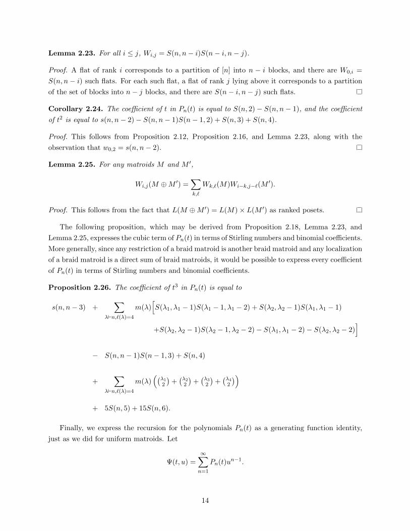
Lemma 2.23. For all i ≤ j, Wi,j = S(n, n− i)S(n− i, n− j).

Proof. A flat of rank i corresponds to a partition of [n] into n − i blocks, and there are W0,i =

S(n, n− i) such flats. For each such flat, a flat of rank j lying above it corresponds to a partition

of the set of blocks into n− j blocks, and there are S(n− i, n− j) such flats.

Corollary 2.24. The coefficient of t in Pn(t) is equal to S(n, 2)− S(n, n− 1), and the coefficient

of t2 is equal to s(n, n− 2)− S(n, n− 1)S(n− 1, 2) + S(n, 3) + S(n, 4).

Proof. This follows from Proposition 2.12, Proposition 2.16, and Lemma 2.23, along with the

observation that w0,2 = s(n, n− 2).

Lemma 2.25. For any matroids M and M ′,

Wi,j(M ⊕M ′) =∑k,`

Wk,`(M)Wi−k,j−`(M′).

Proof. This follows from the fact that L(M ⊕M ′) = L(M)× L(M ′) as ranked posets.

The following proposition, which may be derived from Proposition 2.18, Lemma 2.23, and

Lemma 2.25, expresses the cubic term of Pn(t) in terms of Stirling numbers and binomial coefficients.

More generally, since any restriction of a braid matroid is another braid matroid and any localization

of a braid matroid is a direct sum of braid matroids, it would be possible to express every coefficient

of Pn(t) in terms of Stirling numbers and binomial coefficients.

Proposition 2.26. The coefficient of t3 in Pn(t) is equal to

s(n, n− 3) +∑

λ`n,`(λ)=4

m(λ)[S(λ1, λ1 − 1)S(λ1 − 1, λ1 − 2) + S(λ2, λ2 − 1)S(λ1, λ1 − 1)

+S(λ2, λ2 − 1)S(λ2 − 1, λ2 − 2)− S(λ1, λ1 − 2)− S(λ2, λ2 − 2)]

− S(n, n− 1)S(n− 1, 3) + S(n, 4)

+∑

λ`n,`(λ)=4

m(λ)((

λ1

2

)+(λ2

2

)+(λ3

2

)+(λ4

2

))

+ 5S(n, 5) + 15S(n, 6).

Finally, we express the recursion for the polynomials Pn(t) as a generating function identity,

just as we did for uniform matroids. Let

Ψ(t, u) =

∞∑n=1

Pn(t)un−1.

14

For any partition ν (of any number), let ν be the partition of |ν| + `(ν) obtained by adding 1 to

each of the parts of ν.

Proposition 2.27. We have

Ψ(t−1, tu) =∑ν

m(ν)u|ν|−1ν1∏j=1

(t− j)νtj · ∂

|ν|u

|ν|!

(u|ν|+1Ψ(t, u)

),

where the sum is over all partitions ν of any size.

Proof. Our defining recursion tells us that

Ψ(t−1, tu) =

∞∑n=1

Pn(t−1)tn−1un−1 =

∞∑n=1

∑λ`n

m(λ)P`(λ)(t)

λ1−1∏j=1

(t− j)λtj+1

un−1

=∑λ

m(λ)P`(λ)(t)u|λ|−1

λ1−1∏j=1

(t− j)λtj+1 .

(We adopt the convention that P0(t) = 0 so that the empty partition contributes nothing to the

sum.) For any partition ν, let νk be the partition obtained by adding k new parts of size 1 to ν.

We will replace the sum over λ with a sum over ν and k, with λ = νk. Note that we have

m(λ) =

(|νk||ν|

)m(ν), `(λ) = `(ν) + k, λ1 − 1 = ν1, and λtj+1 = νtj ,

thus we can rewrite our equation as

Ψ(t−1, tu) =∑ν

∞∑k=0

(|νk||ν|

)m(ν)P`(ν)+k(t)u

|νk|−1ν1∏j=1

(t− j)νtj

=∑ν

m(ν)u|ν|ν1∏j=1

(t− j)νtj ·∞∑k=0

(|νk||ν|

)P`(ν)+k(t)u

`(ν)+k−1.

Next, we observe that (|νk||ν|

)u`(ν)+k−1 = u`(ν)−1∂

|ν|u

|ν|!u|νk|,

so

Ψ(t−1, tu) =∑ν

m(ν)u|ν|ν1∏j=1

(t− j)νtj ·∞∑k=0

u`(ν)−1∂|ν|u

|ν|!u|νk|P`(ν)+k(t)

=∑ν

m(ν)u|ν|−1ν1∏j=1

(t− j)νtj · ∂

|ν|u

|ν|!

(u|ν|+1

∞∑k=0

u`(ν)+k−1P`(ν)+k(t)

)

=∑ν

m(ν)u|ν|−1ν1∏j=1

(t− j)νtj · ∂

|ν|u

|ν|!

(u|ν|+1Ψ(t, u)

).

15

This completes the proof.

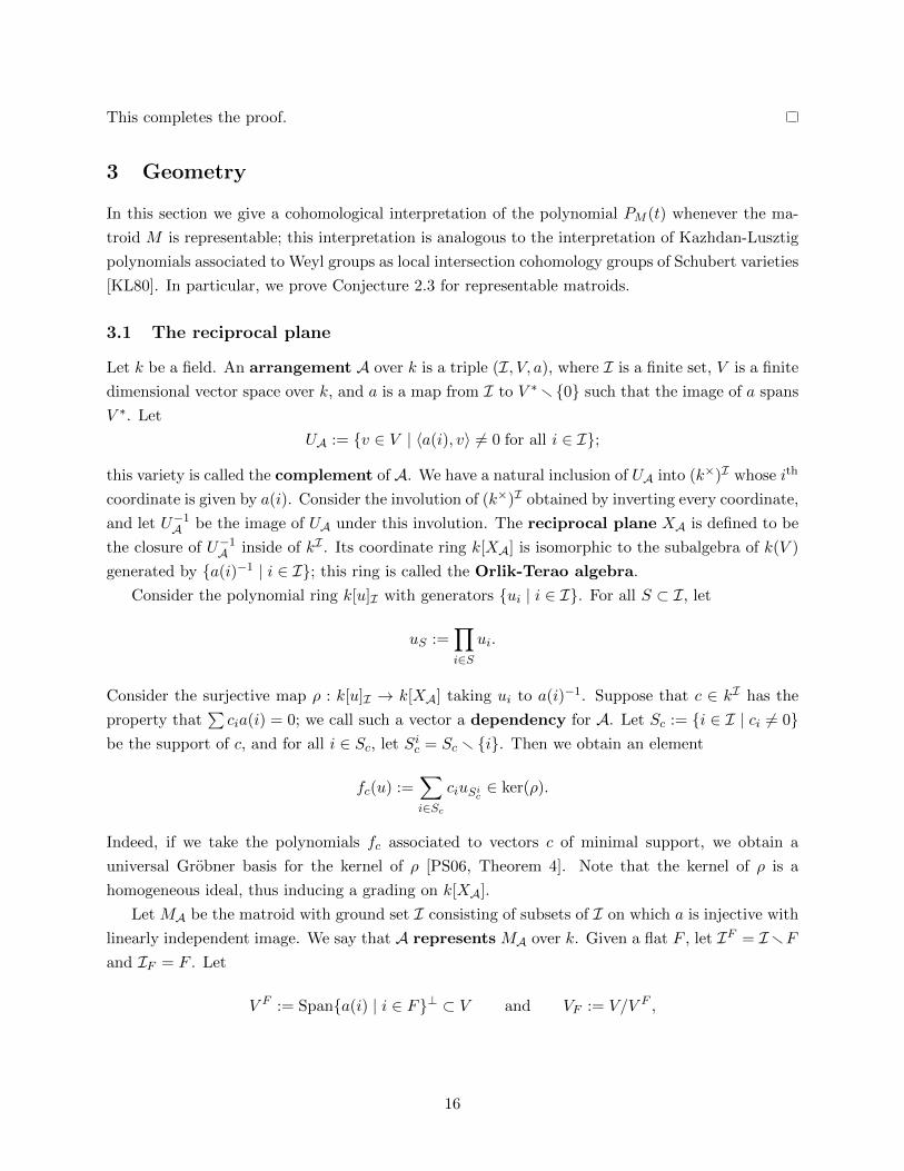
3 Geometry

In this section we give a cohomological interpretation of the polynomial PM (t) whenever the ma-

troid M is representable; this interpretation is analogous to the interpretation of Kazhdan-Lusztig

polynomials associated to Weyl groups as local intersection cohomology groups of Schubert varieties

[KL80]. In particular, we prove Conjecture 2.3 for representable matroids.

3.1 The reciprocal plane

Let k be a field. An arrangement A over k is a triple (I, V, a), where I is a finite set, V is a finite

dimensional vector space over k, and a is a map from I to V ∗r {0} such that the image of a spans

V ∗. Let

UA := {v ∈ V | 〈a(i), v〉 6= 0 for all i ∈ I};

this variety is called the complement of A. We have a natural inclusion of UA into (k×)I whose ith

coordinate is given by a(i). Consider the involution of (k×)I obtained by inverting every coordinate,

and let U−1A be the image of UA under this involution. The reciprocal plane XA is defined to be

the closure of U−1A inside of kI . Its coordinate ring k[XA] is isomorphic to the subalgebra of k(V )

generated by {a(i)−1 | i ∈ I}; this ring is called the Orlik-Terao algebra.

Consider the polynomial ring k[u]I with generators {ui | i ∈ I}. For all S ⊂ I, let

uS :=∏i∈S

ui.

Consider the surjective map ρ : k[u]I → k[XA] taking ui to a(i)−1. Suppose that c ∈ kI has the

property that∑cia(i) = 0; we call such a vector a dependency for A. Let Sc := {i ∈ I | ci 6= 0}

be the support of c, and for all i ∈ Sc, let Sic = Sc r {i}. Then we obtain an element

fc(u) :=∑i∈Sc

ciuSic ∈ ker(ρ).

Indeed, if we take the polynomials fc associated to vectors c of minimal support, we obtain a

universal Grobner basis for the kernel of ρ [PS06, Theorem 4]. Note that the kernel of ρ is a

homogeneous ideal, thus inducing a grading on k[XA].

Let MA be the matroid with ground set I consisting of subsets of I on which a is injective with

linearly independent image. We say that A represents MA over k. Given a flat F , let IF = IrFand IF = F . Let

V F := Span{a(i) | i ∈ F}⊥ ⊂ V and VF := V/V F ,

16

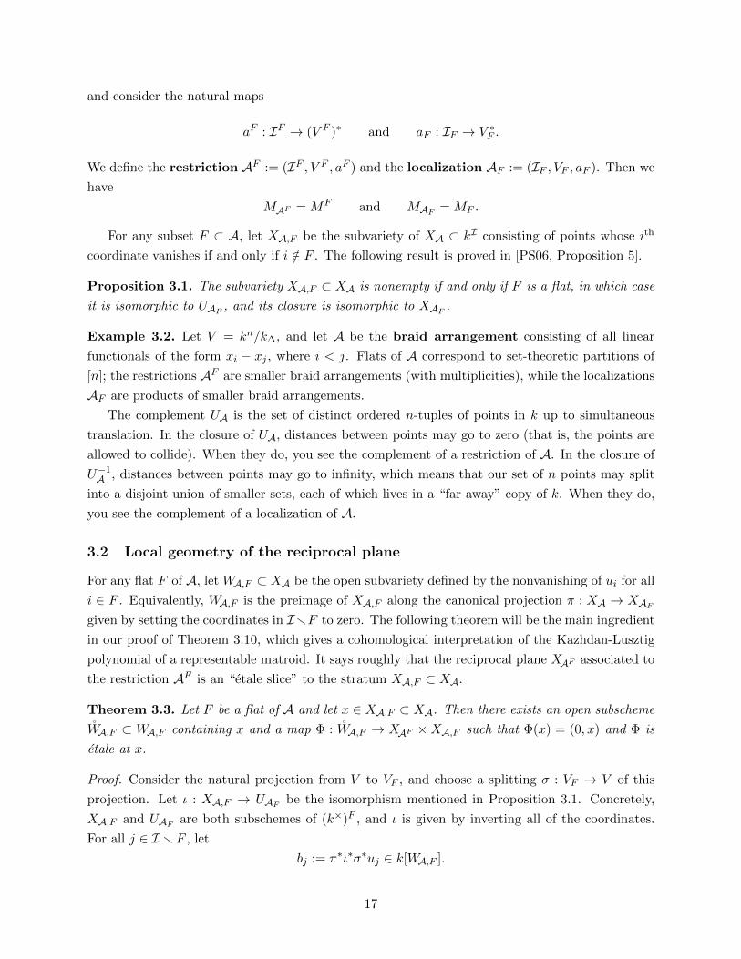
and consider the natural maps

aF : IF → (V F )∗ and aF : IF → V ∗F .

We define the restriction AF := (IF , V F , aF ) and the localization AF := (IF , VF , aF ). Then we

have

MAF = MF and MAF = MF .

For any subset F ⊂ A, let XA,F be the subvariety of XA ⊂ kI consisting of points whose ith

coordinate vanishes if and only if i /∈ F . The following result is proved in [PS06, Proposition 5].

Proposition 3.1. The subvariety XA,F ⊂ XA is nonempty if and only if F is a flat, in which case

it is isomorphic to UAF , and its closure is isomorphic to XAF .

Example 3.2. Let V = kn/k∆, and let A be the braid arrangement consisting of all linear

functionals of the form xi − xj , where i < j. Flats of A correspond to set-theoretic partitions of

[n]; the restrictions AF are smaller braid arrangements (with multiplicities), while the localizations

AF are products of smaller braid arrangements.

The complement UA is the set of distinct ordered n-tuples of points in k up to simultaneous

translation. In the closure of UA, distances between points may go to zero (that is, the points are

allowed to collide). When they do, you see the complement of a restriction of A. In the closure of

U−1A , distances between points may go to infinity, which means that our set of n points may split

into a disjoint union of smaller sets, each of which lives in a “far away” copy of k. When they do,

you see the complement of a localization of A.

3.2 Local geometry of the reciprocal plane

For any flat F of A, let WA,F ⊂ XA be the open subvariety defined by the nonvanishing of ui for all

i ∈ F . Equivalently, WA,F is the preimage of XA,F along the canonical projection π : XA → XAFgiven by setting the coordinates in IrF to zero. The following theorem will be the main ingredient

in our proof of Theorem 3.10, which gives a cohomological interpretation of the Kazhdan-Lusztig

polynomial of a representable matroid. It says roughly that the reciprocal plane XAF associated to

the restriction AF is an “etale slice” to the stratum XA,F ⊂ XA.

Theorem 3.3. Let F be a flat of A and let x ∈ XA,F ⊂ XA. Then there exists an open subscheme

WA,F ⊂ WA,F containing x and a map Φ : WA,F → XAF ×XA,F such that Φ(x) = (0, x) and Φ is

etale at x.

Proof. Consider the natural projection from V to VF , and choose a splitting σ : VF → V of this

projection. Let ι : XA,F → UAF be the isomorphism mentioned in Proposition 3.1. Concretely,

XA,F and UAF are both subschemes of (k×)F , and ι is given by inverting all of the coordinates.

For all j ∈ I r F , let

bj := π∗ι∗σ∗uj ∈ k[WA,F ].

17

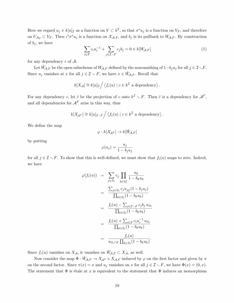
Here we regard uj ∈ k[u]I as a function on V ⊂ kI , so that σ∗uj is a function on VF , and therefore

on UAF ⊂ VF . Then ι∗σ∗uj is a function on XA,F , and bj is its pullback to WA,F . By construction

of bj , we have ∑i∈F

ciu−1i +

∑j∈IrF

cjbj = 0 ∈ k[WA,F ] (1)

for any dependency c of A.

Let WA,F be the open subscheme of WA,F defined by the nonvanishing of 1−bjuj for all j ∈ IrF .

Since uj vanishes at x for all j ∈ I r F , we have x ∈ WA,F . Recall that

k[XA] ∼= k[u]I

/⟨fc(u) | c ∈ kI a dependency

⟩.

For any dependency c, let c be the projection of c onto kI r F . Then c is a dependency for AF ,

and all dependencies for AF arise in this way, thus

k[XAF ] ∼= k[u]IrF

/⟨fc(u) | c ∈ kI a dependency

⟩.

We define the map

ϕ : k[XAF ]→ k[WA,F ]

by putting

ϕ(uj) =uj

1− bjujfor all j ∈ I rF . To show that this is well-defined, we must show that fc(u) maps to zero. Indeed,

we have

ϕ(fc(u)) =∑j∈Sc

cj∏k∈Sjc

uk1− bkuk

=

∑j∈Sc cjuSjc

(1− bjuj)∏k∈Sc(1− bkuk)

=fc(u)−

∑j∈IrF cjbj uSc∏

k∈Sc(1− bkuk)

=fc(u) +

∑i∈F ciu

−1i uSc∏

k∈Sc(1− bkuk)

=fc(u)

uSc∩F∏k∈Sc(1− bkuk)

.

Since fc(u) vanishes on XA, it vanishes on WA,F ⊂ XA, as well.

Now consider the map Φ : WA,F → XAF ×XA,F induced by ϕ on the first factor and given by π

on the second factor. Since π(x) = x and uj vanishes on x for all j ∈ I rF , we have Φ(x) = (0, x).

The statement that Φ is etale at x is equivalent to the statement that Φ induces an isomorphism

18

on tangent cones. Indeed, the tangent cone of XAF × XA,F at (0, x) is isomorphic to XAF × VF ,

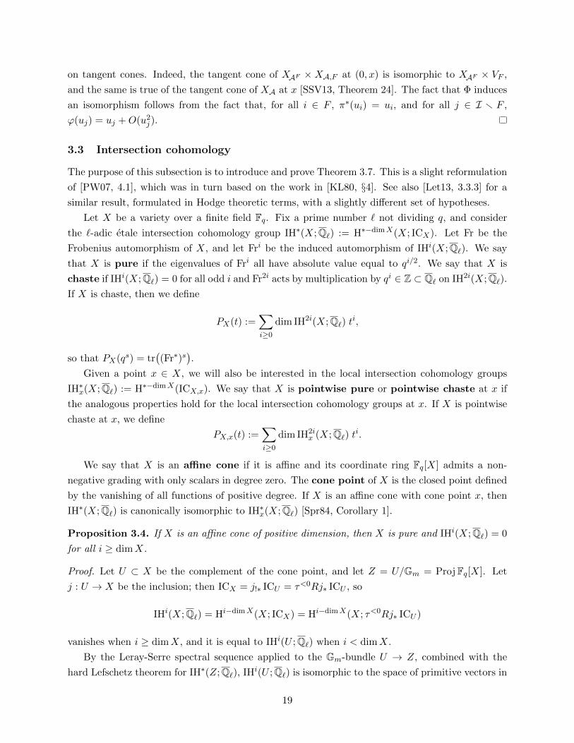
and the same is true of the tangent cone of XA at x [SSV13, Theorem 24]. The fact that Φ induces

an isomorphism follows from the fact that, for all i ∈ F , π∗(ui) = ui, and for all j ∈ I r F ,

ϕ(uj) = uj +O(u2j ).

3.3 Intersection cohomology

The purpose of this subsection is to introduce and prove Theorem 3.7. This is a slight reformulation

of [PW07, 4.1], which was in turn based on the work in [KL80, §4]. See also [Let13, 3.3.3] for a

similar result, formulated in Hodge theoretic terms, with a slightly different set of hypotheses.

Let X be a variety over a finite field Fq. Fix a prime number ` not dividing q, and consider

the `-adic etale intersection cohomology group IH∗(X;Q`) := H∗−dimX(X; ICX). Let Fr be the

Frobenius automorphism of X, and let Fri be the induced automorphism of IHi(X;Q`). We say

that X is pure if the eigenvalues of Fri all have absolute value equal to qi/2. We say that X is

chaste if IHi(X;Q`) = 0 for all odd i and Fr2i acts by multiplication by qi ∈ Z ⊂ Q` on IH2i(X;Q`).

If X is chaste, then we define

PX(t) :=∑i≥0

dim IH2i(X;Q`) ti,

so that PX(qs) = tr((Fr∗)s

).

Given a point x ∈ X, we will also be interested in the local intersection cohomology groups

IH∗x(X;Q`) := H∗−dimX(ICX,x). We say that X is pointwise pure or pointwise chaste at x if

the analogous properties hold for the local intersection cohomology groups at x. If X is pointwise

chaste at x, we define

PX,x(t) :=∑i≥0

dim IH2ix (X;Q`) t

i.

We say that X is an affine cone if it is affine and its coordinate ring Fq[X] admits a non-

negative grading with only scalars in degree zero. The cone point of X is the closed point defined

by the vanishing of all functions of positive degree. If X is an affine cone with cone point x, then

IH∗(X;Q`) is canonically isomorphic to IH∗x(X;Q`) [Spr84, Corollary 1].

Proposition 3.4. If X is an affine cone of positive dimension, then X is pure and IHi(X;Q`) = 0

for all i ≥ dimX.

Proof. Let U ⊂ X be the complement of the cone point, and let Z = U/Gm = ProjFq[X]. Let

j : U → X be the inclusion; then ICX = j!∗ ICU = τ<0Rj∗ ICU , so

IHi(X;Q`) = Hi−dimX(X; ICX) = Hi−dimX(X; τ<0Rj∗ ICU )

vanishes when i ≥ dimX, and it is equal to IHi(U ;Q`) when i < dimX.

By the Leray-Serre spectral sequence applied to the Gm-bundle U → Z, combined with the

hard Lefschetz theorem for IH∗(Z;Q`), IHi(U ;Q`) is isomorphic to the space of primitive vectors in

19

IH∗(Z;Q`) for all i < dimX. Thus purity of X follows from purity of the projective variety Z.

Remark 3.5. Proposition 3.4 is well-known to experts; in particular, a version of the argument

above can also be found in [BJ04, 4.2] and [dCM09, 3.1].

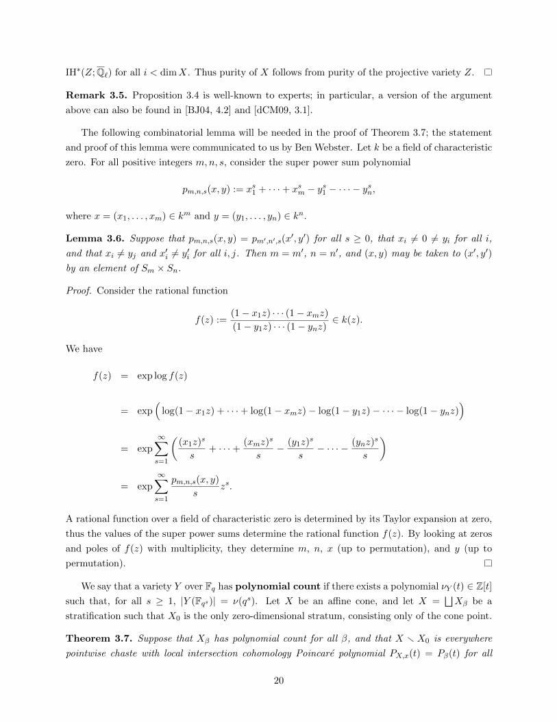
The following combinatorial lemma will be needed in the proof of Theorem 3.7; the statement

and proof of this lemma were communicated to us by Ben Webster. Let k be a field of characteristic

zero. For all positive integers m,n, s, consider the super power sum polynomial

pm,n,s(x, y) := xs1 + · · ·+ xsm − ys1 − · · · − ysn,

where x = (x1, . . . , xm) ∈ km and y = (y1, . . . , yn) ∈ kn.

Lemma 3.6. Suppose that pm,n,s(x, y) = pm′,n′,s(x′, y′) for all s ≥ 0, that xi 6= 0 6= yi for all i,

and that xi 6= yj and x′i 6= y′i for all i, j. Then m = m′, n = n′, and (x, y) may be taken to (x′, y′)

by an element of Sm × Sn.

Proof. Consider the rational function

f(z) :=(1− x1z) · · · (1− xmz)(1− y1z) · · · (1− ynz)

∈ k(z).

We have

f(z) = exp log f(z)

= exp(

log(1− x1z) + · · ·+ log(1− xmz)− log(1− y1z)− · · · − log(1− ynz))

= exp∞∑s=1

((x1z)

s

s+ · · ·+ (xmz)

s

s− (y1z)

s

s− · · · − (ynz)

s

s

)

= exp∞∑s=1

pm,n,s(x, y)

szs.

A rational function over a field of characteristic zero is determined by its Taylor expansion at zero,

thus the values of the super power sums determine the rational function f(z). By looking at zeros

and poles of f(z) with multiplicity, they determine m, n, x (up to permutation), and y (up to

permutation).

We say that a variety Y over Fq has polynomial count if there exists a polynomial νY (t) ∈ Z[t]

such that, for all s ≥ 1, |Y (Fqs)| = ν(qs). Let X be an affine cone, and let X =⊔Xβ be a

stratification such that X0 is the only zero-dimensional stratum, consisting only of the cone point.

Theorem 3.7. Suppose that Xβ has polynomial count for all β, and that X r X0 is everywhere

pointwise chaste with local intersection cohomology Poincare polynomial PX,x(t) = Pβ(t) for all

20

x ∈ Xβ. Then X is chaste (and therefore also pointwise chaste at the cone point), and

tdimXPX(t−1) =∑β

νXβ (t)Pβ(t).

Proof. Consider the Frobenius automorphism Fr∗c of IH∗c(X;Q`), the compactly supported inter-

section cohomology group. By Poincare duality [KW01, II.7.3], we have

qsdimX tr(

(Fr∗)−s y IH2 dimX−i(X;Q`))

= tr(

(Fr∗c)s y IHi

c(X;Q`)).

By the Lefschetz formula [KW01, III.12.1(4)], we have∑i≥0

(−1)i tr(

(Fr∗c)s y IHi

c(X;Q`))

=∑

x∈X(Fqs )

∑i≥0

(−1)i tr(

(Fr∗x)s y IH∗x(X;Q`)).

If x ∈ Xβ(Fqs) for some β 6= 0, then x contributes Pβ(qs) to this sum. If x is the cone point, then

IH∗x(X;Q`) ∼= IH∗(X;Q`), so x contributes∑

(−1)i tr((Fr∗)s y IHi(X;Q`)

). Thus we have∑

i≥0

(−1)i(qsdimX tr

((Fr∗)−s y IH2 dimX−i(X;Q`)

)− tr

((Fr∗)s y IHi(X;Q`)

))=∑β 6=0

νXβ (qs)Pβ(qs).

(2)

Let ri = dim IHi(X;Q`), and let α1,i, · · · , αri,i be the eigenvalues of Fr∗ y IHi(X;Q`), counted

with multiplicity. Write

αi := (αi,1, · · · , αi,ri) and qdimX/αi := (qdimX/αi,1, · · · , qdimX/αi,ri),

so that the left-hand side of Equation (2) is equal to∑i≥0

(−1)ipri,ri,s(qdimX/α, α).

The right-hand side is a polynomial in qs with integer coefficients, and therefore can be written

in the form pm,n,s(x, y), where the entries of x and y are all non-negative powers of q and the

powers that appear in x are distinct from the powers that appear in y. Assuming that dimX > 0,

Proposition 3.4 tells us that the entries of αi are disjoint from the entries of qdimX/αi, thus the

hypotheses of Lemma 3.6 are satisfied and each αi,j is equal to a power of q. Since we already know

that X is pure, this implies that X is chaste, and Equation (2) becomes

qsdimXPX(q−s)− PX(qs) =∑β 6=0

νXβ (qs)Pβ(qs).

Since this holds for all s, we may replace qs with the variable t. Moving PX(t) = P0(t) to the

right-hand side, and noting that νX0(t) = 1, we obtain the desired equality.

21

3.4 Cohomological interpretation of Kazhdan-Lusztig polynomials

We now combine the results of Subsections 3.1, 3.2, and 3.3 to give a cohomological interpretation

of the polynomial PMA(t). Let A be an arrangement over a finite field Fq, and let ` be a prime

that does not divide q.

Lemma 3.8. For every flat F and every element x ∈ XA,F , IH∗x(XA;Q`) ∼= IH∗(XAF ;Q`).

Proof. By Theorem 3.3, we have an etale map from a neighborhood of x ∈ XA to a neighborhood of

(0, x) ∈ XAF ×XA,F . It follows that the local intersection cohomology of XA at x is isomorphic to

the local intersection cohomology of XAF at the cone point times the local intersection cohomology

of XA,F at x. By the contraction lemma [Spr84, Corollary 1], the local intersection cohomology of

XAF at the cone point is isomorphic to the the global intersection cohomology of XAF . Since XA,F

is smooth, the local intersection cohomology of XA,F is trivial.

Let χA(t) = χMA(t) be the characteristic polynomial of A. The variety UA is polynomial count

with νUA(t) = χA(t) [OT92, 2.69]. For any arrangement A in V , let

rkA := rkMA = dimV = dimXA.

Proposition 3.9. The reciprocal plane XA is chaste, and

trkAPXA(t−1) =∑F

χAF (t)PXAF(t).

Proof. We proceed by induction on the rank of A. If rkA = 0, the statement is trivial. Now assume

that the proposition holds for all arrangements of smaller rank. In particular, this means that XAF

is chaste for all nonempty flats F . By Lemma 3.8, this implies that XA is pointwise chaste away

from the cone point, with PXA,x(t) = PXAF(t) for all F nonempty and x ∈ XA,F . The statement

then follows from Theorem 3.7.

As a consequence, we find that the intersection cohomology Poincare polynomial of a recipro-

cal plane over a finite field coincides with the Kazhdan-Lusztig polynomial of the corresponding

matroid.

Theorem 3.10. If A is an arrangement over a finite field, then PXA(t) = PMA(t).

Proof. This follows from Proposition 3.4, Theorem 3.9, and the uniqueness of Theorem 2.2.

Corollary 3.11. If a matroid M is representable, then PM (t) has non-negative coefficients.

Proof. If M is representable over some field, then it is representable over a finite field [Rad57,

Theorems 4 & 6], and the corollary follows from Theorem 3.10.

LetA be an arrangement over C. Theorem 3.10 says that we may interpret PMA(t) geometrically

by choosing a representation of MA over a finite field and considering the `-adic etale intersection

22

cohomology of the resulting reciprocal plane. However, one might prefer to think about the topo-

logical intersection cohomology groups of XA(C). Let PXA(t) =∑

i≥0 dim IH2i(XA(C);C) ti.

Proposition 3.12. If A is an arrangement over C, then the topological intersection cohomology

of XA(C) vanishes in odd degree, and PXA(t) = PMA(t). Furthermore, the topological analogue of

Lemma 3.8 holds.

Proof. Choose a spreading out of XA and then base change to a finite field Fq of sufficiently

large characteristic. The fact that the topological intersection cohomology of XA(C) coincides

with the graded dimension of the `-adic etale intersection cohomology of XA(Fq) after tensoring

with C follows from [BBD82, 6.1.9] (see also [Con, 1.4.8.1]). The same goes for local intersection

cohomology groups.

Remark 3.13. For A an arrangement over a finite field or C, the isomorphism class of the variety

XA is not determined by the matroid MA. However, Theorem 3.10 and Proposition 3.12 imply

that the intersection cohomology Poincare polynomial PXA(t) is determined by MA.

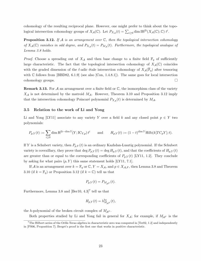
3.5 Relation to the work of Li and Yong

Li and Yong [LY11] associate to any variety Y over a field k and any closed point p ∈ Y two

polynomials:

Pp,Y (t) :=∑i≥0

dim H2i−dimY(Y ; ICY,p) ti and Hp,Y (t) := (1− t)dimY Hilb(k[TCpY ]; t).

If Y is a Schubert variety, then Pp,Y (t) is an ordinary Kazhdan-Lusztig polynomial. If the Schubert

variety is covexillary, they prove that degPp,Y (t) = degHp,Y (t), and that the coefficients of Hp,Y (t)

are greater than or equal to the corresponding coefficients of Pp,Y (t) [LY11, 1.2]. They conclude

by asking for what pairs (p, Y ) this same statement holds [LY11, 7.1].

If A is an arrangement over k = Fq or C, Y = XA, and p ∈ XA,F , then Lemma 3.8 and Theorem

3.10 (if k = Fq) or Proposition 3.12 (if k = C) tell us that

Pp,Y (t) = PMAF(t).

Furthermore, Lemma 3.8 and [Ber10, 4.3]7 tell us that

Hp,Y (t) = hbcMAF

(t),

the h-polynomial of the broken circuit complex of MAF .

Both properties studied by Li and Yong fail in general for XA; for example, if MAF is the

7The Hilbert series of the Orlik-Terao algebra in characteristic zero was computed in [Ter02, 1.2] and independentlyin [PS06, Proposition 7]; Berget’s proof is the first one that works in positive characteristic.

23

uniform matroid of rank d on a set of cardinality d+ 1, we have

hbcMAF

(t) = 1 + t+ t2 + · · ·+ td−1,

while PMAF(t) is a polynomial of degree less than d

2 with linear coefficient equal to(d+1

2

)− (d+ 1)

(Corollary 2.20). It would be interesting to determine whether there is a nice class of “covexillary

matroids” for which hbcM (t) dominates PM (t).

4 Algebra

In this section we define a q-deformation of the Mobius algebra of a matroid, use Kazhdan-Lusztig

polynomials to define a special basis for this algebra, and conjecture that the structure coefficients

for this basis are non-negative. We then verify the conjecture for Boolean matroids, and for uniform

matroids and braid matroids of rank at most 3.

4.1 The deformed Mobius algebra

Fix a matroid M . The Mobius algebra is defined to be the free abelian group

E(M) := Z{εF | F ∈ L(M)}

equipped with the multiplication εF · εG := εF∨G. We define a deformation

Eq(M) := Z[q, q−1]{εF | F ∈ L(M)}

with multiplication

εF · εG :=∑

H≥I≥F∨Gµ(I,H) qcrk I εH ,

where crk I := rkM − rk I is the corank of I. The fact that we recover our original multiplication

when q = 1 follows from the fact that∑

H≥I≥F∨G µ(I,H) = δ(H,F ∨G).

Proposition 4.1. The Z[q, q−1]-algebra Eq(M) is commutative, associative, and unital, with unit

equal to ∑F≤G

µ(F,G) q− crkF εG.

Proof. Commutativity is immediate from the definition. For associativity, we note that

εF · εG =∑

H≥I≥F∨Gµ(I,H) qcrk I εH

=∑H,I

ζ(F, I)ζ(G, I)µ(I,H) qcrk I εH ,

24

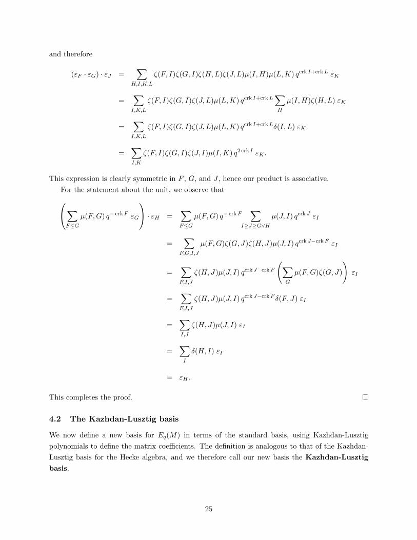
and therefore

(εF · εG) · εJ =∑

H,I,K,L

ζ(F, I)ζ(G, I)ζ(H,L)ζ(J, L)µ(I,H)µ(L,K) qcrk I+crkL εK

=∑I,K,L

ζ(F, I)ζ(G, I)ζ(J, L)µ(L,K) qcrk I+crkL∑H

µ(I,H)ζ(H,L) εK

=∑I,K,L

ζ(F, I)ζ(G, I)ζ(J, L)µ(L,K) qcrk I+crkLδ(I, L) εK

=∑I,K

ζ(F, I)ζ(G, I)ζ(J, I)µ(I,K) q2 crk I εK .

This expression is clearly symmetric in F , G, and J , hence our product is associative.

For the statement about the unit, we observe that∑F≤G

µ(F,G) q− crkF εG

· εH =∑F≤G

µ(F,G) q− crkF∑

I≥J≥G∨Hµ(J, I) qcrk J εI

=∑

F,G,I,J

µ(F,G)ζ(G, J)ζ(H,J)µ(J, I) qcrk J−crkF εI

=∑F,I,J

ζ(H,J)µ(J, I) qcrk J−crkF

(∑G

µ(F,G)ζ(G, J)

)εI

=∑F,I,J

ζ(H,J)µ(J, I) qcrk J−crkF δ(F, J) εI

=∑I,J

ζ(H,J)µ(J, I) εI

=∑I

δ(H, I) εI

= εH .

This completes the proof.

4.2 The Kazhdan-Lusztig basis

We now define a new basis for Eq(M) in terms of the standard basis, using Kazhdan-Lusztig

polynomials to define the matrix coefficients. The definition is analogous to that of the Kazhdan-

Lusztig basis for the Hecke algebra, and we therefore call our new basis the Kazhdan-Lusztig

basis.

25

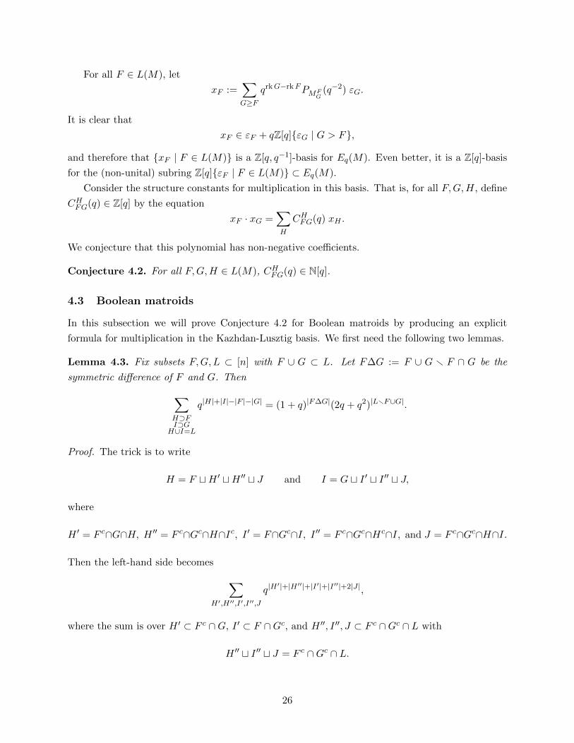
For all F ∈ L(M), let

xF :=∑G≥F

qrkG−rkFPMFG

(q−2) εG.

It is clear that

xF ∈ εF + qZ[q]{εG | G > F},

and therefore that {xF | F ∈ L(M)} is a Z[q, q−1]-basis for Eq(M). Even better, it is a Z[q]-basis

for the (non-unital) subring Z[q]{εF | F ∈ L(M)} ⊂ Eq(M).

Consider the structure constants for multiplication in this basis. That is, for all F,G,H, define

CHFG(q) ∈ Z[q] by the equation

xF · xG =∑H

CHFG(q) xH .

We conjecture that this polynomial has non-negative coefficients.

Conjecture 4.2. For all F,G,H ∈ L(M), CHFG(q) ∈ N[q].

4.3 Boolean matroids

In this subsection we will prove Conjecture 4.2 for Boolean matroids by producing an explicit

formula for multiplication in the Kazhdan-Lusztig basis. We first need the following two lemmas.

Lemma 4.3. Fix subsets F,G,L ⊂ [n] with F ∪ G ⊂ L. Let F∆G := F ∪ G r F ∩ G be the

symmetric difference of F and G. Then∑H⊃FI⊃G

H∪I=L

q|H|+|I|−|F |−|G| = (1 + q)|F∆G|(2q + q2)|LrF∪G|.

Proof. The trick is to write

H = F tH ′ tH ′′ t J and I = G t I ′ t I ′′ t J,

where

H ′ = F c∩G∩H, H ′′ = F c∩Gc∩H∩Ic, I ′ = F∩Gc∩I, I ′′ = F c∩Gc∩Hc∩I, and J = F c∩Gc∩H∩I.

Then the left-hand side becomes ∑H′,H′′,I′,I′′,J

q|H′|+|H′′|+|I′|+|I′′|+2|J |,

where the sum is over H ′ ⊂ F c ∩G, I ′ ⊂ F ∩Gc, and H ′′, I ′′, J ⊂ F c ∩Gc ∩ L with

H ′′ t I ′′ t J = F c ∩Gc ∩ L.

26

We have ∑H′,I′

q|H′|+|I′| = (1 + q)|F∆G|,

and, for each fixed J , ∑H′′,I′′

q|H′′|+|I′′| = (2q)|F

c∩Gc∩L∩Jc|.

Thus the left-hand side is equal to

(1 + q)|F∆G|∑

J⊂F c∩Gc∩Lq2|J |(2q)|F

c∩Gc∩L∩Jc| = (1 + q)|F∆G|(2q + q2)|Fc∩Gc∩L|,

where the last equality is an application of the binomial theorem.

Lemma 4.4. Fix subsets F ⊂ G ⊂ [n]. Then for any polynomials f(q) and g(q), we have

∑F⊂H⊂G

f(q)|GrH|g(q)|HrF | =(f(q) + g(q)

)|GrF |.

Proof. This is simply a reformulation of the binomial theorem.

Proposition 4.5. Let M be the Boolean matroid on the ground set [n]. Then for any subsets

F,G ⊂ [n], we have

xF · xG =∑

K⊃F∪Gqn−|K|(1 + q)|K|−|F∩G| xK .

Proof. For each F ⊂ G, MFG is again Boolean, so PMF

G(t) = 1 by Corollary 2.10. This means that

xF =∑G⊃F

q|GrF | εG,

and, by Mobius inversion,

εF =∑G⊃F

(−q)|GrF | xG.

We therefore have

xF · xG =

(∑H⊃F

q|HrF |εH

)·

(∑I⊃G

q|IrG|εI

)

=∑H⊃FI⊃G

q|H|+|I|−|F |−|G| εH · εI

=∑H⊃FI⊃G

q|H|+|I|−|F |−|G|∑

J⊃H∪Iqn−|J |(1− q)|JrH∪I| εJ

=∑H⊃FI⊃G

q|H|+|I|−|F |−|G|∑

J⊃H∪Iqn−|J |(1− q)|JrH∪I|

∑K⊃J

(−q)|KrJ | xK .

27

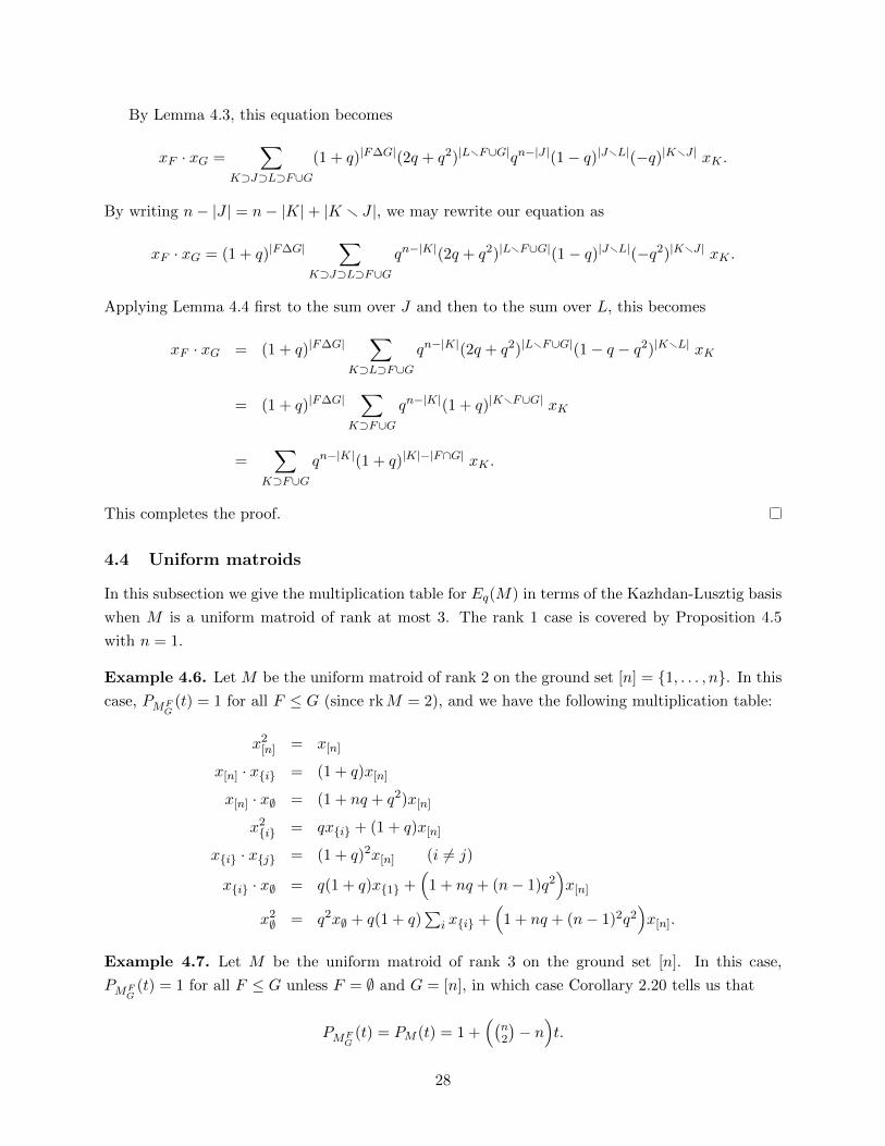
By Lemma 4.3, this equation becomes

xF · xG =∑

K⊃J⊃L⊃F∪G(1 + q)|F∆G|(2q + q2)|LrF∪G|qn−|J |(1− q)|JrL|(−q)|KrJ | xK .

By writing n− |J | = n− |K|+ |K r J |, we may rewrite our equation as

xF · xG = (1 + q)|F∆G|∑

K⊃J⊃L⊃F∪Gqn−|K|(2q + q2)|LrF∪G|(1− q)|JrL|(−q2)|KrJ | xK .

Applying Lemma 4.4 first to the sum over J and then to the sum over L, this becomes

xF · xG = (1 + q)|F∆G|∑

K⊃L⊃F∪Gqn−|K|(2q + q2)|LrF∪G|(1− q − q2)|KrL| xK

= (1 + q)|F∆G|∑

K⊃F∪Gqn−|K|(1 + q)|KrF∪G| xK

=∑

K⊃F∪Gqn−|K|(1 + q)|K|−|F∩G| xK .

This completes the proof.

4.4 Uniform matroids

In this subsection we give the multiplication table for Eq(M) in terms of the Kazhdan-Lusztig basis

when M is a uniform matroid of rank at most 3. The rank 1 case is covered by Proposition 4.5

with n = 1.

Example 4.6. Let M be the uniform matroid of rank 2 on the ground set [n] = {1, . . . , n}. In this

case, PMFG

(t) = 1 for all F ≤ G (since rkM = 2), and we have the following multiplication table:

x2[n] = x[n]

x[n] · x{i} = (1 + q)x[n]

x[n] · x∅ = (1 + nq + q2)x[n]

x2{i} = qx{i} + (1 + q)x[n]

x{i} · x{j} = (1 + q)2x[n] (i 6= j)

x{i} · x∅ = q(1 + q)x{1} +(

1 + nq + (n− 1)q2)x[n]

x2∅ = q2x∅ + q(1 + q)

∑i x{i} +

(1 + nq + (n− 1)2q2

)x[n].

Example 4.7. Let M be the uniform matroid of rank 3 on the ground set [n]. In this case,

PMFG

(t) = 1 for all F ≤ G unless F = ∅ and G = [n], in which case Corollary 2.20 tells us that

PMFG

(t) = PM (t) = 1 +((

n2

)− n

)t.

28

We have the following multiplication table:

x2[n] = x[n]

x[n] · x{i,j} = (1 + q)x[n]

x[n] · xi =(

1 + (n− 1)q + q2)x[n]

x[n] · x∅ =(

1 +(n2

)q +

(n2

)q2 + q3

)x[n]

x{i,j} · x{i,j} = qx{i,j} + (1 + q)x[n]

x{i,j} · x{i,k} = (1 + q)2x[n] (j 6= k)

x{i,j} · x{k,`} = (1 + q)2x[n] ({i, j} ∩ {k, `} = ∅)

x{i,j} · x{i} = q(1 + q)x{i,j} +(

1 + (n− 1)q + (n− 2)q2)x[n]

x{i,j} · xk = (1 + nq + nq2 + q3)x[n] (k /∈ {i, j})

x{i,j} · x∅ = q(1 + q)2x{i,j} +(

1 +(n2

)q + (n2 − n− 3)q2 +

((n2

)− 2)q3)x[n]

x2{i} = q2x{i} + q(1 + q)

∑j 6=i x{i,j} +

(1 + (n− 1)q + (n− 2)2q2

)x[n]

x{i}x{j} = q(1 + q)2x{i,j} +(

1 + (2n− 3)q + n(n− 2)q2 + (2n− 5)q3)x[n] (i 6= j)

x{i} · x∅ = q2(1 + q)xi + q(1 + q)2∑j 6=i x{i,j}

+(

1 +(n2

)q + 1

2(n− 1)(n2 − 6)q2 + 12(n− 1)(n2 − 8)q3 + 1

2n(n− 3)q4)x[n]

x2∅ = q3x∅ + q2(1 + q)

∑i x{i} + q(1 + q)2

∑i<j x{i,j}

+(

1 +(n2

)q + 1

4n(n3 − 2n2 − n− 2)q2 + 12(n− 1)(n3 − n2 − 5n− 2)q3

+14n

2(n+ 1)(n− 3)q4 + 12n(n− 3)q5

)x[n].

Note that each coefficient is non-negative for all n ≥ 3, and when n = 3, this multiplication table

agrees with Proposition 4.5.

Remark 4.8. It is reasonable to ask if Conjecture 4.2 would still hold if we were to redefine the

Kazhdan-Lusztig basis by putting xF :=∑

G≥F qrkG−rkF εG; that is, if we were to pretend that

all Kazhdan-Lusztig polynomials were equal to 1. If we did this, the linear term of C[n]∅∅ (q) in

Example 4.7 would be equal to 2n−(n2

), which is negative when n > 5. Thus the Kazhdan-Lusztig

polynomials truly play a necessary role in Conjecture 4.2.

4.5 Braid matroids

Finally, we consider braid matroids of small rank. The braid matroid M2 is isomorphic to the

Boolean matroid of rank 1. The braid matroid M3 is isomorphic to the uniform matroid of rank 2

on the ground set [3].

Example 4.9. Let M4 be the braid arrangement of rank 3. The ground set I has cardinality(42

)= 6, and PM4(t) = 1 + t (see appendix). Flats correspond to set theoretic partitions of [4].

29

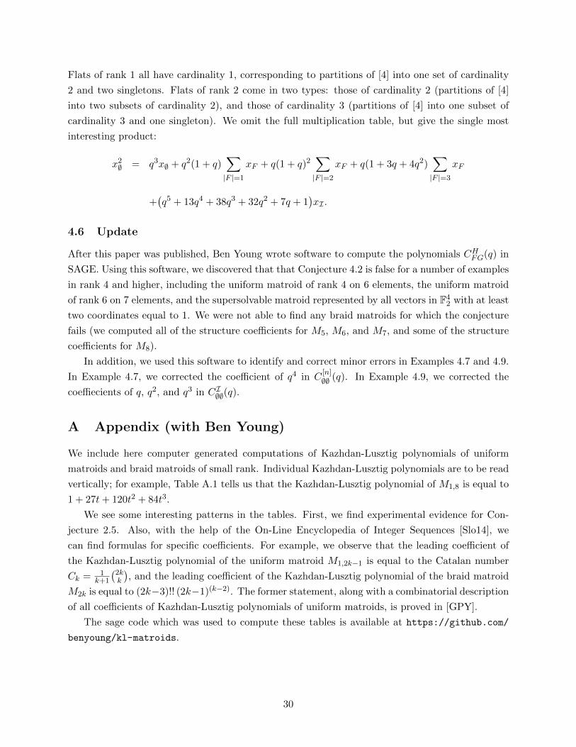
Flats of rank 1 all have cardinality 1, corresponding to partitions of [4] into one set of cardinality

2 and two singletons. Flats of rank 2 come in two types: those of cardinality 2 (partitions of [4]

into two subsets of cardinality 2), and those of cardinality 3 (partitions of [4] into one subset of

cardinality 3 and one singleton). We omit the full multiplication table, but give the single most

interesting product:

x2∅ = q3x∅ + q2(1 + q)

∑|F |=1

xF + q(1 + q)2∑|F |=2

xF + q(1 + 3q + 4q2)∑|F |=3

xF

+(q5 + 13q4 + 38q3 + 32q2 + 7q + 1

)xI .

4.6 Update

After this paper was published, Ben Young wrote software to compute the polynomials CHFG(q) in

SAGE. Using this software, we discovered that that Conjecture 4.2 is false for a number of examples

in rank 4 and higher, including the uniform matroid of rank 4 on 6 elements, the uniform matroid

of rank 6 on 7 elements, and the supersolvable matroid represented by all vectors in F42 with at least

two coordinates equal to 1. We were not able to find any braid matroids for which the conjecture

fails (we computed all of the structure coefficients for M5, M6, and M7, and some of the structure

coefficients for M8).

In addition, we used this software to identify and correct minor errors in Examples 4.7 and 4.9.

In Example 4.7, we corrected the coefficient of q4 in C[n]∅∅ (q). In Example 4.9, we corrected the

coeffiecients of q, q2, and q3 in CI∅∅(q).

A Appendix (with Ben Young)

We include here computer generated computations of Kazhdan-Lusztig polynomials of uniform

matroids and braid matroids of small rank. Individual Kazhdan-Lusztig polynomials are to be read

vertically; for example, Table A.1 tells us that the Kazhdan-Lusztig polynomial of M1,8 is equal to

1 + 27t+ 120t2 + 84t3.

We see some interesting patterns in the tables. First, we find experimental evidence for Con-

jecture 2.5. Also, with the help of the On-Line Encyclopedia of Integer Sequences [Slo14], we

can find formulas for specific coefficients. For example, we observe that the leading coefficient of

the Kazhdan-Lusztig polynomial of the uniform matroid M1,2k−1 is equal to the Catalan number

Ck = 1k+1

(2kk

), and the leading coefficient of the Kazhdan-Lusztig polynomial of the braid matroid

M2k is equal to (2k−3)!! (2k−1)(k−2). The former statement, along with a combinatorial description

of all coefficients of Kazhdan-Lusztig polynomials of uniform matroids, is proved in [GPY].

The sage code which was used to compute these tables is available at https://github.com/

benyoung/kl-matroids.

30

A.1 Uniform matroids

Table 1: Kazhdan-Lusztig polynomials for the uniform matroid M1,d

d = 1 2 3 4 5 6 7 8 9 10 11 12 13 14 15

1 1 1 1 1 1 1 1 1 1 1 1 1 1 1 1

t 2 5 9 14 20 27 35 44 54 65 77 90 104

t2 5 21 56 120 225 385 616 936 1365 1925 2640

t3 14 84 300 825 1925 4004 7644 13650 23100

t4 42 330 1485 5005 14014 34398 76440

t5 132 1287 7007 28028 91728

t6 429 5005 32032

t7 1430

Table 2: Kazhdan-Lusztig polynomials for the uniform matroid M2,d

d = 3 4 5 6 7 8 9 10 11 12 13 14 15

1 1 1 1 1 1 1 1 1 1 1 1 1 1

t 5 14 28 48 75 110 154 208 273 350 440 544 663

t2 21 98 288 675 1375 2541 4368 7098 11025 16500 23936

t3 84 552 2145 6380 16016 35672 72618 137760 246840

t4 330 2805 13585 49049 146510 382200 899640

t5 1287 13442 78078 331968 1150968

t6 5005 62062 420784

t7 19448

Table 3: Kazhdan-Lusztig polynomials for the uniform matroid M3,d

d = 3 4 5 6 7 8 9 10 11 12 13 14

1 1 1 1 1 1 1 1 1 1 1 1 1

t 9 28 62 117 200 319 483 702 987 1350 1804 2363

t2 56 288 927 2365 5214 10374 19110 33138 54720 86768

t3 300 2145 9020 28886 77714 184730 399840 803760

t4 1485 13585 70499 271635 862680 2384760

t5 7007 78078 482118 2171988

t6 32032 420784

31

A.2 Braid matroids

Table 4: Kazhdan-Lusztig polynomials for the braid matroid Mn

n = 1 2 3 4 5 6 7 8 9 10 11 12 13

1 1 1 1 1 1 1 1 1 1 1 1 1 1

t 1 5 16 42 99 219 466 968 1981 4017

t2 15 175 1225 6769 32830 147466 632434 2637206

t3 735 16065 204400 2001230 16813720 128172330

t4 76545 2747745 56143395 864418555

t5 13835745 746080335

n = 14 15 16 17

1 1 1 1 1

t 8100 16278 32647 65399

t2 10811801 43876001 176981207 711347303

t3 915590676 6252966720 41362602281 267347356003

t4 11200444255 129344350135 1377269949055 13819966094935

t5 22495833360 502627875750 9305666915545 151395489770525

t6 3859590735 293349030975 12290930276625 376566883537845

t7 1539272109375 157277996100225

n = 18 19 20

1 1 1 1

t 130918 261972 524097

t2 2853229952 11430715476 45762931992

t3 1698735206324 10656703437054 66208557177786

t4 132618161185510 1229703907984734 11100857399288280

t5 2242336712846230 30941776173508200 404180066561961690

t6 9443716601138820 205809448675350520 4042252614171772000

t7 8758018896026400 352844128436870070 11522756204094885750

t8 831766748637825 110176255068905025 7879824460254822075

t9 585243816844111425

References

[Aig87] Martin Aigner, Whitney numbers, Combinatorial geometries, Encyclopedia Math. Appl.,

vol. 29, Cambridge Univ. Press, Cambridge, 1987, pp. 139–160.

[Bac79] Kenneth Baclawski, The Mobius algebra as a Grothendieck ring, J. Algebra 57 (1979),

no. 1, 167–179.

32

[BB81] Alexandre Beılinson and Joseph Bernstein, Localisation de g-modules, C. R. Acad. Sci.

Paris Ser. I Math. 292 (1981), no. 1, 15–18.

[BB05] Anders Bjorner and Francesco Brenti, Combinatorics of Coxeter groups, Graduate Texts

in Mathematics, vol. 231, Springer, New York, 2005.

[BBD82] A. A. Beilinson, J. Bernstein, and P. Deligne, Faisceaux pervers, Analysis and topology

on singular spaces, I (Luminy, 1981), Asterisque, vol. 100, Soc. Math. France, Paris, 1982,

pp. 5–171.

[Ber10] Andrew Berget, Products of linear forms and Tutte polynomials, European J. Combin.

31 (2010), no. 7, 1924–1935.

[BJ04] Michel Brion and Roy Joshua, Intersection cohomology of reductive varieties, J. Eur.

Math. Soc. (JEMS) 6 (2004), no. 4, 465–481.

[BK81] J.-L. Brylinski and M. Kashiwara, Kazhdan-Lusztig conjecture and holonomic systems,

Invent. Math. 64 (1981), no. 3, 387–410.

[Con] Brian Conrad, Etale cohomology, lecture notes available online.

[dCM09] Mark Andrea A. de Cataldo and Luca Migliorini, The decomposition theorem, perverse

sheaves and the topology of algebraic maps, Bull. Amer. Math. Soc. (N.S.) 46 (2009),

no. 4, 535–633.

[DW75] Thomas A. Dowling and Richard M. Wilson, Whitney number inequalities for geometric

lattices, Proc. Amer. Math. Soc. 47 (1975), 504–512.

[EW14] Ben Elias and Geordie Williamson, The Hodge theory of Soergel bimodules, Ann. of Math.

(2) 180 (2014), no. 3, 1089–1136.

[GPY] Katie Gedeon, Nicholas Proudfoot, and Ben Young, The equivariant Kazhdan-Lusztig

polynomial of a matroid, preprint.

[GZ83] Curtis Greene and Thomas Zaslavsky, On the interpretation of Whitney numbers through

arrangements of hyperplanes, zonotopes, non-Radon partitions, and orientations of

graphs, Trans. Amer. Math. Soc. 280 (1983), no. 1, 97–126.

[HK12] June Huh and Eric Katz, Log-concavity of characteristic polynomials and the Bergman

fan of matroids, Math. Ann. 354 (2012), no. 3, 1103–1116.

[KL79] David Kazhdan and George Lusztig, Representations of Coxeter groups and Hecke alge-

bras, Invent. Math. 53 (1979), no. 2, 165–184.

[KL80] David Kazhdan and George Lusztig, Schubert varieties and Poincare duality, Geometry

of the Laplace operator (Proc. Sympos. Pure Math., Univ. Hawaii, Honolulu, Hawaii,

33

1979), Proc. Sympos. Pure Math., XXXVI, Amer. Math. Soc., Providence, R.I., 1980,

pp. 185–203.

[Koo06] Woong Kook, On the product of log-concave polynomials, Integers 6 (2006), A40, 4.

[Kun86] Joseph P. S. Kung, Radon transforms in combinatorics and lattice theory, Combinatorics

and ordered sets (Arcata, Calif., 1985), Contemp. Math., vol. 57, Amer. Math. Soc.,

Providence, RI, 1986, pp. 33–74.

[KW01] Reinhardt Kiehl and Rainer Weissauer, Weil conjectures, perverse sheaves and l’adic

Fourier transform, Ergebnisse der Mathematik und ihrer Grenzgebiete. 3. Folge. A Series

of Modern Surveys in Mathematics [Results in Mathematics and Related Areas. 3rd Series.

A Series of Modern Surveys in Mathematics], vol. 42, Springer-Verlag, Berlin, 2001.

[Let13] Emmanuel Letellier, Quiver varieties and the character ring of general linear groups over

finite fields, J. Eur. Math. Soc. (JEMS) 15 (2013), no. 4, 1375–1455.

[Lus83] G. Lusztig, Left cells in Weyl groups, Lie group representations, I (College Park, Md.,

1982/1983), Lecture Notes in Math., vol. 1024, Springer, Berlin, 1983, pp. 99–111.

[LY11] Li Li and Alexander Yong, Kazhdan-Lusztig polynomials and drift configurations, Algebra

Number Theory 5 (2011), no. 5, 595–626.

[OT92] Peter Orlik and Hiroaki Terao, Arrangements of hyperplanes, Grundlehren der Mathe-

matischen Wissenschaften [Fundamental Principles of Mathematical Sciences], vol. 300,

Springer-Verlag, Berlin, 1992.

[Pol99] Patrick Polo, Construction of arbitrary Kazhdan-Lusztig polynomials in symmetric

groups, Represent. Theory 3 (1999).

[PS06] Nicholas Proudfoot and David Speyer, A broken circuit ring, Beitrage Algebra Geom. 47

(2006), no. 1, 161–166.

[PW07] Nicholas Proudfoot and Ben Webster, Intersection cohomology of hypertoric varieties, J.

Algebraic Geom. 16 (2007), no. 1, 39–63.

[Rad57] R. Rado, Note on independence functions, Proc. London Math. Soc. (3) 7 (1957), 300–320.

[Slo14] N. J. A. Sloane, The On-Line Encyclopedia of Integer Sequences, 2014, http://oeis.org.

[Sol67] Louis Solomon, The Burnside algebra of a finite group, J. Combinatorial Theory 2 (1967),

603–615.

[Spr84] T. A. Springer, A purity result for fixed point varieties in flag manifolds, J. Fac. Sci. Univ.

Tokyo Sect. IA Math. 31 (1984), no. 2, 271–282.

34

[SSV13] Raman Sanyal, Bernd Sturmfels, and Cynthia Vinzant, The entropic discriminant, Adv.

Math. 244 (2013), 678–707.

[Ter02] Hiroaki Terao, Algebras generated by reciprocals of linear forms, J. Algebra 250 (2002),

no. 2, 549–558.

[Wak] Max Wakefield, Partial flag incidence algebras, preprint.

35