the joy of factorization at large n
TRANSCRIPT
Prepared for submission to JHEP
The joy of factorization at large N :
five-dimensional indices and AdS black holes
Seyed Morteza Hosseini,a,b Itamar Yaakovc and Alberto Zaffaronic,d
aDepartment of Physics, Imperial College London, London, SW7 2AZ, UKbKavli IPMU (WPI), UTIAS, The University of Tokyo, Kashiwa, Chiba 277-8583, JapancINFN, sezione di Milano-Bicocca, I-20126 Milano, ItalydDipartimento di Fisica, Universita di Milano-Bicocca, I-20126 Milano, Italy
E-mail: [email protected], [email protected],
Abstract: We discuss the large N factorization properties of five-dimensional super-
symmetric partition functions for CFT with a holographic dual. We consider partition
functions on manifolds of the form M = M3 × S2ε , where ε is an equivariant parameter
for rotation. We show that, when M3 is a squashed three-sphere, the large N partition
functions can be obtained by gluing elementary blocks associated with simple physical
quantities. The same is true for various observables of the theories on M3 = Σg × S1,
where Σg is a Riemann surface of genus g, and, with a natural assumption on the form of
the saddle point, also for the partition function, corresponding to either the topologically
twisted index or a mixed one. This generalizes results in three and four dimensions and
correctly reproduces the entropy of known black objects in AdS6 ×w S4 and AdS7 × S4.
We also provide the supersymmetric background and explicitly perform localization for
the mixed index on Σg × S1 × S2ε , filling a gap in the literature.ar
Xiv
:211
1.03
069v
1 [
hep-
th]
4 N
ov 2
021
Contents
1 Introduction 2
2 Generalities about factorization 5
2.1 The entropy functional 5
2.2 Factorization in field theory 8
3 Factorization of the S3b × S2
ε partition function 10
3.1 USp(2N) gauge theory with matter 12
3.2 N = 2 super Yang-Mills 15
4 Refined topologically twisted index 19
4.1 Alternative interpretations for W(S2ε×S1)×R2 21
4.2 W(S2ε×S1)×R2 and its factorization 24
4.3 Factorization of the index 31
5 A mixed index on (S2ε × S1)×Σg 37
5.1 Rigid supergravity background 37
5.2 Localization 40
5.3 Derivation of the partition function 45
5.4 W(S2ε×S1)×R2 and its factorization 52
5.5 Factorization of the index 57
6 An index theorem for the twisted and mixed matrix models 61
7 Discussion and outlook 64
A Refined S3b × S2
ε partition function 65
B Asymptotic behavior of q-functions 66
C Supersymmetry conventions 67
C.1 Spinor conventions 67
C.2 Rigid minimal 5d conformal supergravity 68
C.3 Matter multiplet transformations 70
– 1 –

1 Introduction
There has been recently a lot of progress in the microscopic derivation of the entropy of
anti de Sitter (AdS) black holes, starting with the magnetically charged and topologi-
cally twisted ones in AdS4×S7 [1] and followed by the Kerr-Newman (KN) black holes in
AdS5×S5 [2–4]. This analysis has been extended to many other black objects in AdSd, with
d = 4, 5, 6, 7 with different types of electromagnetic charges and rotations and with various
amounts of supersymmetry. For a (partial) review, see [5]. A general entropy functional
that captures the large N entropy of black holes and black strings in general AdS compact-
ifications with a holographic dual was written in [6]. In this picture, the entropy functional
is a sum of universal contributions called gravitational blocks, which can be related to some
simple field theory quantity, either the central charge or the sphere-partition function of
the dual conformal field theory (CFT). The proposal has been successfully tested for all
known examples in maximally supersymmetric compactifications and in many other cases
with less supersymmetry. The microscopic counting of states for black objects in AdS is
usually done by a large N saddle point analysis of a supersymmetric index in the dual
CFT. Black hole physics then suggests that, in the large N limit, the corresponding field
theory partition functions should factorize and the CFT free energy
FM ≡ − logZM , (1.1)
where M is the Euclidean boundary of the black object, should be the sum of universal
contributions associated to a geometric description ofM as the gluing of elementary pieces.
The form of the entropy functional in [6] was indeed suggested by the decomposition of the
supersymmetric partition functions in holomorphic blocks [7].1 In this paper, we call this
property large N factorization. For a more precise definition see below and the beginning
of section 2.
All recent field theory computations for black objects in AdS4 and AdS5 have confirmed
the above picture. The factorization properties are particularly nontrivial when magnetic
charges and rotation are simultaneously present, see for example [20] for rotating black
strings in AdS5 × S5, and [21] for a class of rotating black holes in AdS4.
In this paper we analyse the large N factorization properties of five-dimensional par-
tition functions on various manifolds of the formM =M3×S2ε , where ε is an equivariant
parameter for rotations along S2 and a chemical potential for the angular momentum of
the dual black hole. We will consider three examples. The first is the partition function on
S3b × S2
ε , with a squashing along S3 and a topological twist along S2 [22]. Although there
is no associated dual black object, we expect factorization to hold nevertheless. The other
two examples correspond to partition functions on (S2ε ×S1)×Σg, with a topological twist
along the genus g Riemann surface Σg, and a different type of supersymmetry. When
S2 is twisted this is the (partially) refined five-dimensional topologicallly twisted index
1The idea of “gluing” or “sewing” building blocks to compose field theory observables is old and it has
been successfully used in many different contexts. See [8–19] for developments related to our context.
– 2 –

discussed in [22, 23]. The case where S2 is not twisted corresponds to a mixed index, first
considered in [24].
All these partition functions can be written, for genus 0, by gluing copies of the
Nekrasov’s partition functions [25], in the spirit of [8]. Since a proper derivation of the
mixed index is lacking in the literature we provide it here, by identifying the supergravity
background the five-dimensional field theory should be coupled to in order to preserve
supersymmetry and by performing an explicit localization around this background.
For simplicity, we will focus on two specific field theories, the so-called ENf+1 Seiberg
theory, the UV fixed point of a N = 1 USp(2N) gauge theory coupled to Nf fundamental
hypermultiplets and an antisymmetric one [26], and the N = 2 SU(N) super Yang-Mills
(SYM) theory, which is supposed to flow at strong coupling to the six-dimensional N =
(2, 0) theory of type AN−1. The two theories are holographically dual to the warped
AdS6×w S4 solution in massive type IIA [27], and to AdS7×S4 in M-theory, respectively.
Black holes and black strings in these compactifications have been found in [28–34] and all
the corresponding entropy functionals satisfy factorization. In this paper we investigate
the factorization properties from the field theory point of view. We will verify that various
quantum field theory observables can be written as a sum over two contributions associated
with the two hemispheres of S2
2∑σ=1
B(∆(σ), ε(σ)) =F(∆i + ε
2ti)
ε±F(∆i − ε
2ti)
ε, (1.2)
where ∆i, i = 1, 2 are (constrained) chemical potentials for a U(1) flavor symmetry asso-
ciated with a rotation on S4, ti are the corresponding (constrained) flavor magnetic fluxes
on the sphere S2, and F has a natural interpretation in terms of the central charge/sphere
partition function of the dual CFT. Factorization takes the simple form (1.2) only when
written in terms of constrained variables. If there is a topological twist on S2, correspond-
ing to dual magnetically charged and twisted black holes, we need to use the minus sign
in (1.2) and the constraints2
∆1 +∆2 = 2π , t1 + t2 = 2 , (1.3)
while, if S2 is untwisted, corresponding to dyonic KN black holes, we need to use the plus
sign in (1.2) and the constraints
∆1 +∆2 = 2π + ε , t1 + t2 = 0 . (1.4)
The expression (1.2) is clearly reminiscent of an equivariant localization formula.
In the various examples F is proportional to3
2In some examples, S3b × S2
ε for instance, we will normalize the first constraint as ∆1 + ∆2 = 2 to
facilitate comparison with literature.3For the explicit formulae and normalization factors see (3.23) and (3.40), for S3
b ×S2ε , (4.74) and (4.89)
for the twisted index, and (5.101) and (5.117) for the mixed one.
– 3 –
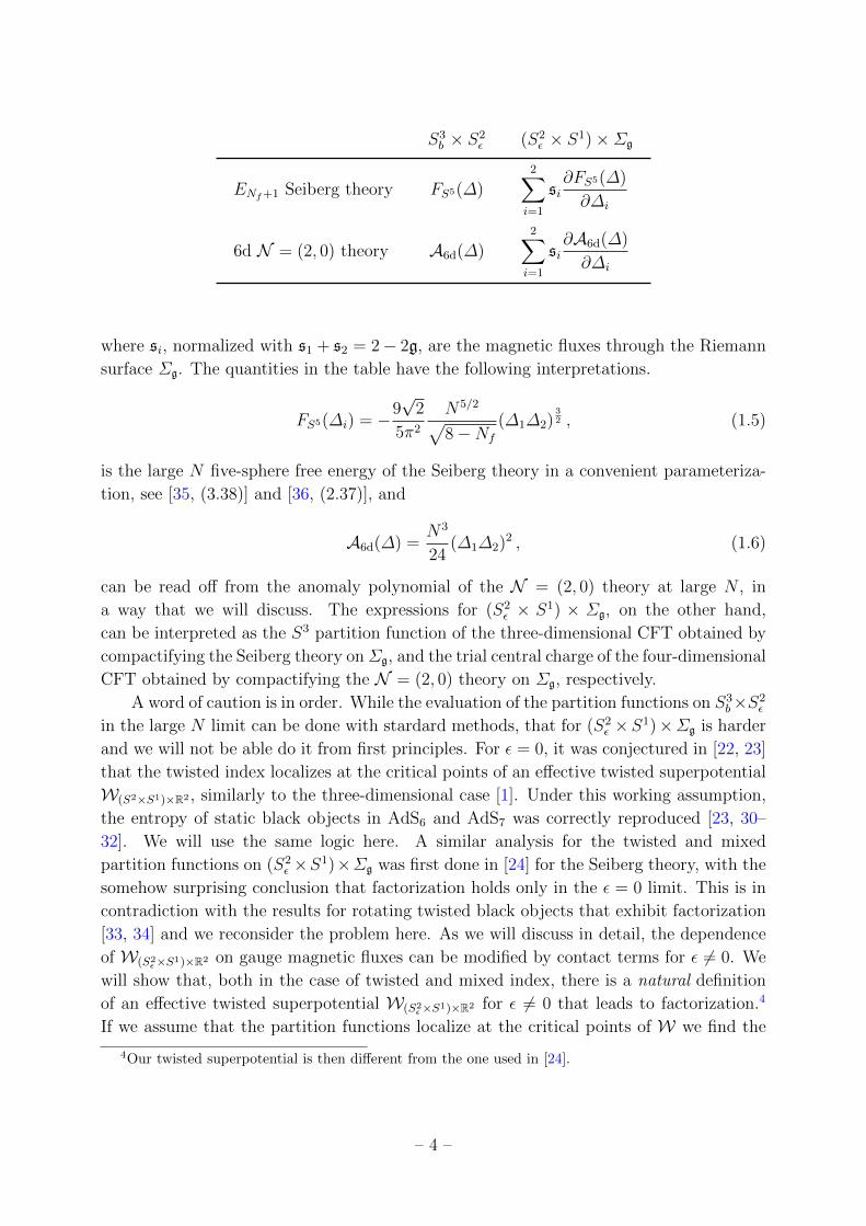
S3b × S2
ε (S2ε × S1)×Σg
ENf+1 Seiberg theory FS5(∆)2∑i=1
si∂FS5(∆)
∂∆i
6d N = (2, 0) theory A6d(∆)2∑i=1
si∂A6d(∆)
∂∆i
where si, normalized with s1 + s2 = 2− 2g, are the magnetic fluxes through the Riemann
surface Σg. The quantities in the table have the following interpretations.
FS5(∆i) = −9√
2
5π2
N5/2√8−Nf
(∆1∆2)32 , (1.5)
is the large N five-sphere free energy of the Seiberg theory in a convenient parameteriza-
tion, see [35, (3.38)] and [36, (2.37)], and
A6d(∆) =N3
24(∆1∆2)2 , (1.6)
can be read off from the anomaly polynomial of the N = (2, 0) theory at large N , in
a way that we will discuss. The expressions for (S2ε × S1) × Σg, on the other hand,
can be interpreted as the S3 partition function of the three-dimensional CFT obtained by
compactifying the Seiberg theory onΣg, and the trial central charge of the four-dimensional
CFT obtained by compactifying the N = (2, 0) theory on Σg, respectively.
A word of caution is in order. While the evaluation of the partition functions on S3b×S2
ε
in the large N limit can be done with stardard methods, that for (S2ε ×S1)×Σg is harder
and we will not be able do it from first principles. For ε = 0, it was conjectured in [22, 23]
that the twisted index localizes at the critical points of an effective twisted superpotential
W(S2×S1)×R2 , similarly to the three-dimensional case [1]. Under this working assumption,
the entropy of static black objects in AdS6 and AdS7 was correctly reproduced [23, 30–
32]. We will use the same logic here. A similar analysis for the twisted and mixed
partition functions on (S2ε ×S1)×Σg was first done in [24] for the Seiberg theory, with the
somehow surprising conclusion that factorization holds only in the ε = 0 limit. This is in
contradiction with the results for rotating twisted black objects that exhibit factorization
[33, 34] and we reconsider the problem here. As we will discuss in detail, the dependence
of W(S2ε×S1)×R2 on gauge magnetic fluxes can be modified by contact terms for ε 6= 0. We
will show that, both in the case of twisted and mixed index, there is a natural definition
of an effective twisted superpotential W(S2ε×S1)×R2 for ε 6= 0 that leads to factorization.4
If we assume that the partition functions localize at the critical points of W we find the
4Our twisted superpotential is then different from the one used in [24].
– 4 –
free energy quoted above. As we will show, this result correctly reproduces the entropy
of all known black objects in AdS6 and AdS7. It would be nice to have a first principle
derivation of logZM that does not involve the assumptions made in [22–24].
One other interesting result of our analysis is that the on-shell superpotentialW(S2ε×S1)×R2
itself factorizes with blocks given by (1.5) or (1.6).5 Indeed, we have the interesting relation
logZ(S2ε×S1)×Σg(∆, t, ε, s) = i
2∑i=1
si∂W(S2
ε×S1)×R2(∆, t, ε)
∂∆i
, (1.7)
which is the five-dimensional generalization of the index theorem proved in [37, 38].
The paper is organized as follows. In section 2, we will discuss general facts about
factorization and compare results in different dimensions. This will also serve to fix no-
tations and a common ground for the rest of the paper. In section 3, we discuss the
partition function on S3b × S2
ε and we show that it factorizes. In section 4 we discuss the
refined topologically twisted index. We introduce various equivalent definitions of the ef-
fective twisted superpotential W(S2ε×S1)×R2 , and discuss the ambiguity in these definitions.
We then show that, for a natural symmetric choice of W , its on-shell value is factorized.
Moreover, we will verify that, if the partition function localizes at the critical points ofW ,
it also has a factorized form. We will also show that this result correctly reproduces the
entropy of the known rotating twisted black holes in massive IIA [34] and the density of
states of black strings in AdS7×S4 [33]. In section 5, we first write the rigid supergravity
background for the mixed index, and then explicitly perform localization. Using the same
assumptions as in section 4, we show that both the on-shell twisted superpotential and
the partition function factorizes. We also verify that this result correctly reproduces the
entropy of a class of KN black holes in massive IIA [34]. In section 6 we shed light on
the relation between the on-shellW and logZ for the twisted and mixed index by proving
the generalization of the index theorem discussed in [37]. We conclude in section 7 with a
discussion and open problems.
2 Generalities about factorization
In this section we discuss some general facts about factorization in three dimensions, that
we will use also in five dimensions.
2.1 The entropy functional
In the recent and successful approach to microscopic counting, the entropy of supersym-
metric AdS black holes is obtained by extremizing the entropy functional
I(∆i, εa) ≡ logZM(∆i, εa)− i∑i
∆iQi − i∑a
εaJa , (2.1)
5See (4.48) and (4.65) for the twisted index, and (5.77) and (5.88) for the mixed one.
– 5 –

where Qi are the electric charges and Ja the angular momenta. Here, ZM(∆i, εa) is a
supersymmetric partition function on the compact manifold M that depends on a set
of chemical potentials ∆i and εa conjugate to Qi and Ja, respectively. Extra conserved
charges of the black hole, for example magnetic charges, are encoded in the explicit form of
the function ZM(∆i, εa). The entropy functional (2.1) should be extremized with respect
to ∆i and εa. This is the familiar fact that the entropy at zero temperature can be obtained
by taking the Legendre transform of the partition function.
For all known black holes in AdS, supersymmetry imposes a constraint among the
electric charges and the angular momenta. There is a similar linear constraint on the
magnetic charges, if present. It is however convenient to include all possible electric charges
and angular momenta in (2.1) and perform a constrained extremization. In this picture, the
variables ∆i and εa in (2.1) satisfy a linear constraint. This is consistent with the fact that
supersymmetric indices can be only refined with fugacities for symmetries that commute
with a particular supercharge and it allows for a complete field theory description. We
could obviously solve explicitly the constraint and write the entropy functional in terms
of independent variables. However, (2.1) takes a simple form only when written in terms
of constrained variables. In particular, in all known cases, it is a homogeneous function of
degree one of the constrained ∆i and εa.
For all known KN or topologically twisted black holes in maximally supersymmet-
ric AdS compactifications, with or without magnetic charges or rotation, the function
ZM(∆i, εa) in (2.1) can be written as a sum of contributions from the gravitational blocks
[6]
logZM(∆i, εa) =∑σ
B(∆(σ)i , ε(σ)
a ) , (2.2)
where
B(∆(σ)i , ε(σ)
a ) = −F(∆(σ)i )∏
a ε(σ)a
, (2.3)
and each ε(σ)a is a linear combination of the rotational chemical potentials εa while ∆
(σ)i =
∆i ± ipiε(σ), where pi are magnetic fluxes through M.6 Experimentally, σ runs over the
elementary pieces into which the boundary manifoldM is decomposed, in the factorization
of the partition function in holomorphic blocks [7, 16]. Each black hole corresponds to a
different gluing. The function F(∆i) is instead universal, related to the prepotential or
on-shell action of the relevant supergravity, or, more physically, to the large N limit of
the central charge of the dual field theory, in the case of even-dimensional CFTs, or of
the sphere free-energy for odd-dimensional ones, fully refined with respect to the global
symmetries. For the maximal supersymmetric compactifications, F(∆) is proportional to
the values given in table 1.
6One can verify that a straightforward generalization covers also spindle black objects [39–43], see [41]
for an explicit example.
– 6 –

AdS4 × S7 F(∆a) ∝ N3/2√∆1∆2∆3∆4
AdS5 × S5 F(∆a) ∝ N2∆1∆2∆3
AdS6 ×w S4 F(∆a) ∝ N5/3(∆1∆2)3/2
AdS7 × S4 F(∆a) ∝ N3(∆1∆2)2
Table 1: The structure of the block for the AdS backgrounds with maximal allowed
supersymmetry in each dimension. AdS6 ×w S4 is the background dual to the USp(2N)
five-dimensional theory considered in this paper [26, 27]. The chemical potentials ∆i are
associated with the Cartan of the internal sphere isometry in all dimensions.
Let us look at an example which will be also useful in the future. Consider rotating
four-dimensional black holes with a spherical horizon. We can decompose the sphere into
two hemispheres. We then use the A-gluing for topologically twisted black holes
∆(1)i = ∆i +
ε
2pi , ε(1) = ε ,
∆(2)i = ∆i −
ε
2pi , ε(2) = −ε ,
(2.4)
associated with constraints of the form
4∑i=1
∆i = 2 ,4∑i=1
pi = 2 , (2.5)
and the identity gluing (id -gluing)
∆(1)i = ∆i +
ε
2pi , ε(1) = ε ,
∆(2)i = ∆i −
ε
2pi , ε(2) = ε ,
(2.6)
associated with constraints of the form
4∑i=1
∆i − ε = 2π ,4∑i=1
pi = 0 , (2.7)
for KN ones, including dyonic ones. The chemical potentials ∆i are conjugate to the
U(1)4 ⊂ SO(8) isometry for AdS4 × S7 and to a basis of U(1) symmetries Ri in which we
can decompose the general R-symmetry of the model viewed as a generic N = 2 theory.
The constraints on magnetic charges are dictated by supersymmetry: the R-symmetry
magnetic flux must be 2 for the topological twist and zero for KN black holes.
There are two cases where the entropy functional simplifies. The first is the case of KN
black holes in AdSd, d = 4, 5, 6, 7 with no magnetic charges. The corresponding entropy
– 7 –

functional for the maximal supersymmetric compactifications has been written in [44–46].
With zero magnetic fluxes, the gluing formula degenerates and the entropy functional is
the sum of equal contributions, hiding the factorization properties. These become manifest
for dyonic black holes [6, 47].
The second is the case of black objects topologically twisted on S2 but with zero
angular momentum on the sphere. The solution depends on magnetic fluxes si on S2
normalized as∑
i si = 2. We assume that the boundary manifoldM = N × S2 factorizes
into two blocks of the form N×D2, where the disks D2 correspond to the two hemispheres.
Here, we have ε = 0. We can still use the A-gluing defined above, and send ε to zero at
the end of the computation. We obtain
logZM(∆) =∑i
si∂F(∆)
∂∆i
. (2.8)
This is indeed the general structure of the unrefined topologically twisted index at large
N in a variety of situations [1, 23, 37, 38]. The sphere S2 can be replaced with a Riemann
surface Σg of genus g with no major changes and the only difference that now integer
fluxes are normalized as ∑i
si = 2− 2g . (2.9)
In the interesting case where the compactification of the original CFT on the Riemann
surface Σg becomes conformal in the IR,7 (2.8) will express the large N sphere partition
function/central charge of the lower-dimensional CFT in terms of those of the higher-
dimensional one. This relation is for example satisfied for the large N sphere partition
function of the twisted compactification Σg of the ENf+1 Seiberg theory [23, 48]. It is
also a general relation between the large N central charges of theories related by twisted
compactifications, as it can be easily proved by integrating the anomaly polynomial on Σg
[23, 38, 49].
The factorization properties are really nontrivial when magnetic charges and rotation
are simultaneously present. We will focus on this case in the following and in the rest of
the paper.
2.2 Factorization in field theory
The gravitational block picture is expected to be a consequence of analogous factorization
properties of the quantum field theory observables. Let us consider first three dimensions.
Most of the three-dimensional supersymmetric partition functions, and in particular the
topologically twisted index and the superconformal one, can be written by gluing two
holomorphic blocks B(a,∆, ε) according to the formula [7]
Z(∆, ε) =
∫daB(a(1), ∆(1), ε(1))B(a(2), ∆(2), ε(2)) , (2.10)
7Holographically, there exists a domain wall interpolating between AdSp+1 and AdSp−1×Σg, where p
is the dimensionality of the original CFT.
– 8 –
where a(σ), σ = 1, 2, are gauge fugacities. Another useful expression is [7, 16]
Z(∆, ε) =∑α
Bα(∆(1), ε(1))Bα(∆(2), ε(2)) , (2.11)
where α labels a choice of Bethe vacuum for the two-dimensional theory obtained by
reducing the theory on a circle and Bα(∆, ε) =∮
daB(a,∆, ε) is a suitable contour integral
passing through the Bethe vacuum aα. In applications to holography, we typically work
in a saddle point approximation where one particular Bethe vacuum dominates the sum
(2.11) [1]. We then expect some form of factorization also at large N . In a slightly
different but equivalent context, the explicit analysis has been performed in [21] confirming
factorization in the form discussed in the previous section for the topologically twisted
index, the superconformal one, and the sphere partition function, and exploring various
relations among all these quantities.8
To understand the form of (2.3) for generic rotation and magnetic charges, it is con-
venient to expand the holomorphic blocks in the limit of small ε. In this limit, the holo-
morphic blocks are singular (see e.g. [7, (2.22)] and [18, (F.15)])
B(a,∆, ε) ∼ε→0
exp
(− 1
εW(a,∆) + . . .
),
Bα(∆, ε) ∼ε→0
exp
(− 1
εW(aα, ∆) + . . .
),
(2.12)
where W(a,∆) is the effective twisted superpotential of the two-dimensional theory and
the Bethe vacua aα are its critical points. An important point is that, at large N , the
on-shell twisted superpotentialW(aα, ∆) is related to the S3 free energy [21, 37, 38],9 and
the explicit form of the gravitational block (2.3) follows from (2.11). It might seem that
this argument holds only in the strict limit ε→ 0, while in reality (2.3) and the associated
factorization are valid also for ε 6= 0. However, a careful analysis shows that, at large N ,
the subleading terms in (2.12) vanish except for the first one, whose only role is to enforce
the form of the gluing and the constraint among chemical potentials. A similar situation
holds in other dimensions, including five, as we will see.
Analogous results hold for the refined topologically twisted index in four dimensions,
which can be obtained by gluing two copies of T 2 × D2. The index for N = 4 SYM
captures the density of states of rotating black strings in AdS5 × S5 and it has be shown
to factorize both in gravity and field theory in [6, 20]. The field theory computation has
been done by explicitly evaluating the partition function, but the same result would be
obtained using the arguments in [21]. For future reference, let us notice that computation
8The analysis in [21] has been only done, for simplicity, for the N = 8 theory coupled to a fundamental
hypermultiplet, which is supposed to flow to ABJM in the IR, but we might expect the results to hold in
general.9The on-shell twisted superpotential of many three-dimensional N = 2 Chern-Simons-matter gauge
theories with holographic duals were computed in [50–52].
– 9 –

for black strings are usually done in the Cardy limit where the modular parameter τ of the
torus T 2 is small. In this limit the on-shell twisted superpotential of the two-dimensional
theory becomes proportional to the trial central charge of the four-dimensional CFT [38],
W(∆) ∼ a(∆)
τ, (2.13)
in agreement with the general discussion. The Cardy limit on T 2 is appropriate for studying
the physics of the black holes obtained by compactifying the string on a circle, and leads
to the charged Cardy formula [33]. We will encounter a similar setting in section 4.3.2.
For recent results at finite τ see [53].
In five dimensions, the holomorphic blocks B(a,∆, ε1, ε2) are given by the K-theoretic
Nekrasov’s instanton partition function on R2ε1× R2
ε2× S1 [25, 54, 55]. The two chemical
potentials ε1 and ε2 are equivariant parameters for the rotations on R4 and are conjugate
to the two possibile angular momenta for black holes in AdS6 and black strings in AdS7.
All the partition functions we will consider can be written in a similar form to (2.10) by
gluing Nekrasov’s partition functions [19, 22–24]. There are many similarities with three
and four dimensions. The role of the twisted superpotential is played by the Seiberg-
Witten prepotential FSW(a,∆) and the expansion of the holomorphic block is given by
[25]
B(∆, ε1, ε2) ∼ε1,ε2→0
exp
(− 1
ε1ε2FSW(a,∆) + . . .
). (2.14)
Analogy with lower dimensions motivated the conjecture made in [22, 23] that the (un-
refined) five-dimensional partition functions localize at the critical point of FSW(a,∆).
The on-shell value of the Seiberg-Witten prepotential for both the Seiberg theory and the
N = (2, 0) theory has ben computed in [22, 23] and are proportional to the S5 free energy
(1.5) and the anomaly coefficient (1.6), respectively. All these analogies suggest that fac-
torization holds with the blocks given in table 1. Unfortunately, decompositions similar
to (2.11), which would help in setting these statements on a firmer ground, are not fully
understood in five dimensions. We will try to attack directly the five-dimensional matrix
models.
3 Factorization of the S3b × S2
ε partition function
We are interested in evaluating the partition function of five-dimensional N = 1 gauge
theories on S3b×S2
ε in the limits that are appropriate for holography. Here b is the squashing
parameter of the three-sphere and ε is an Ω-deformation on the twisted two-sphere. We
label the (gauge, flavor) fluxes on S2ε by (n, t), respectively. Following [22], for an N = 1
gauge theory with gauge group G, I hypermultiplets in a representation ⊕(RI⊕RI) of the
gauge group, and vanishing Chern-Simons contributions, we can write down the refined
– 10 –

perturbative part of the partition function as (see App.A)10
ZS3b×S2
ε(a, n;∆, t, ε|b) =
1
|W |∑n∈Γh
∮ rk(G)∏i=1
dxi2πixi
e−F
S3b×S2ε
(ai,ni;∆,t,ε|b), (3.1)
where the exponent FS3b×S2
εis given by
FS3b×S2
ε(ai, ni;∆, t, ε|b) =
16π2Q2
g2YM
TrF(na)
+∑α∈G
|Bα|−12∑
`=− |Bα|−12
sign(Bα) logS2
(− iQ (α(a)− 1 + `ε)
∣∣∣b)
−∑I
∑ρI∈RI
|BρI |−12∑
`=− |BρI |−12
sign(BρI ) logS2
(− iQ (ρI(a) + 1− νI(∆) + `ε)
∣∣∣b) .(3.2)
Here, α are the roots of the gauge group, ρ, ν denote the weights of the hypermultiplets
under the gauge and flavor symmetry groups, respectively, and |W | is the order of the
Weyl group of G. Moreover, gYM is the Yang-Mills coupling constant and x = eia. Finally,
S2(z|b) is the double sine function defined by
S2(z|b) ≡∏
m,n∈Z≥0
mb+ nb−1 +Q− iz
mb+ nb−1 +Q+ iz, Q ≡ 1
2
(b+ b−1
), (3.3)
and
Bρ ≡ ρ(n) + ν(t)− 1 Bα ≡ α(n) + 1 . (3.4)
Before moving forward, let us note the following asymptotic relation for the logarithm
of the double sine function, see [56, App. A],11
fb(z) ≡ logS2(z|b) ∼ iπ
(z2
2+Q2
6− 1
12
)sign [Re(z)] , as |Re(z)| → ∞ , (3.5)
that becomes useful when we study the large N limit of the S3b × S2
ε partition function.
Note also that, for a ∈ iR,
sign(B)
|B|−12∑
`=− |B|−12
fb (−iQ(a+ `ε)) = Bfb(−iQa)− iπ(Qε)2
24B(B2 − 1) sign(Im a) . (3.6)
The full partition function on S3b × S2
ε is a sum over instantonic contributions. In the
large N limit, instantons are suppressed and we can restrict to the perturbative part of
the partition function given above.
10One can switch between the conventions used here and those of [22] by setting gthere5 = 12gYM, gthere =
0, uthere = −iQa, νthere = −iQ(1−∆), and mthere − rthere + 1 = n + t− 1.11Recall that sign(0) = 0.
– 11 –
3.1 USp(2N) gauge theory with matter
Let us consider an N = 1 USp(2N) gauge theory coupled to Nf hypermultiplets in the
fundamental representation and one hypermultiplet A in the antisymmetric representation
of USp(2N) [26]. The global symmetry of the theory is SU(2)R×SU(2)A×SO(2Nf )×U(1)Iwhere the first factor is the R-symmetry while the other three factors are flavor symmetries:
SU(2)A acts on A as a doublet, SO(2Nf ) rotates the fundamental hypermultiplets, and
U(1)I is the topological symmetry associated to the conserved instanton number current
j = ∗Tr(F ∧ F ). The global symmetry is enhanced to SU(2)R × SU(2)A × ENf+1 at the
UV fixed point [26]. The theory arises on the intersection of N D4-branes and Nf D8-
branes and orientifold planes, and is holographically dual to the AdS6 ×w S4 background
of massive type IIA supergravity [27] (see also [57–59]).
The partition function on S3b × S2
ε=0 at large N was computed in [22] and scales as
O(N5/2). Here we are interested in the dependence on ε and the factorization properties.
Denote the Cartan elements of USp(2N) by ai, i = 1, . . . , N , and normalize the
weights of the fundamental representation of USp(2N) to be ±ei. The antisymmetric
representation then has weights ±ei ± ej with i > j and N − 1 zero weights, and the
roots are ±ei ± ej with i > j (V1) as well as ±2ei (V2). Vector and hypermultiplets then
contribute to the FS3b×S2
εfunctional
FS3b×S2
ε(ai, ni;∆K , tK , ε|b) = FA+V1(ai, ni;∆m, tm, ε|b) + FF+V2(ai, ni;∆f , tf , ε|b) , (3.7)
with
FA+V1 =N∑i>j
[F∆m, tm(±ai ± aj)−F∆K=2, tK=2(±ai ± aj)
]+ (N − 1)F∆m, tm(0) ,
FF+V2 =N∑i=1
[ Nf∑f=1
F∆f , tf (±ai)−F∆K=2, tK=2(±2ai)
],
(3.8)
where
F∆K , tK (a) ≡ − sign(BK)
|BK |−1
2∑`=− |BK |−1
2
logS2
(− iQ (a+ 1−∆K + `ε)
∣∣∣b) , (3.9)
with BK = n+ tK − 1. Here, the index K labels all the matter fields in the theory and we
introduced the notation
F∆K , tK (±ai) ≡ F∆K , tK (ai, ni) + F∆K , tK (−ai,−ni) . (3.10)
Notice that the vector multiplet contribution is equal to minus the contribution of a
hypermultiplet with ∆K = 2 and tK = 2.
As we will see, the dependence on ∆f is subleading at large N and we will be interested
in the chemical potential ∆m and the flux tm for the Cartan subgroup of SU(2)A. As
– 12 –
mentioned in the introduction, the free energy will take a nice form when written in terms
of constrained variables. We then define
t1 ≡ tm , t2 ≡ 2− tm , s.t.2∑i=1
ti = 2 ,
∆1 ≡ ∆m , ∆2 ≡ 2−∆m , s.t.2∑i=1
∆i = 2 .
(3.11)
Observe that the last term in FA+V1 is of orderO(N) in the large N limit and, given the
expected N5/2 scaling of the free energy, subleading. We will also make a few assumptions
regarding the gauge variables that are true for the solution at ε = 0 [22] and that we will
verify afterwards. Assuming that | Im ai| scales with some positive power of N , and using
(3.5) and (3.6), we obtain12
FA+V1 = iπQ2
N∑i>j
[(∆1t2 +∆2t1)aij −
1
4(4∆1∆2 + ε2t1t2)nij
]sign (Im aij)
+ iπQ2
N∑i>j
[(∆1t2 +∆2t1)a+
ij −1
4(4∆1∆2 + ε2t1t2)n+
ij
]sign
(Im a+
ij
).
(3.12)
For the ease of notation, we defined aij ≡ ai − aj, a+ij ≡ ai + aj and the same for the
gauge fluxes ni. Because of the Weyl reflections of the USp(2N) group, we restrict to
Im ai > 0. Assuming also that the eigenvalues are ordered by increasing imaginary part,
i.e. Im ai > Im aj for i > j, and using
N∑i,j=1
(ai − aj) sign(i− j) = 2N∑j=1
(2j − 1−N)aj ,
N∑i,j=1
(ai + aj) = 2NN∑j=1
aj ,
(3.13)
(3.12) is simplified to
FA+V1 = iπQ2
N∑k=1
(2k − 1)
[(∆1t2 +∆2t1)ak −
1
4(4∆1∆2 + ε2t1t2)nk
]. (3.14)
Similarly, the contribution of FF+V2 to the large N free energy can be computed using
(3.5) and (3.6). It is natural to assume that ai and ni scale with the same positive power
of N . Then, neglecting lower powers of ai and ni that are subleading, we find
FF+V2 = −iπQ2(8−Nf )N∑k=1
(a2k +
ε2
12n2k
)nk . (3.15)
12We do not include subleading terms in the rest of this calculation.
– 13 –

Under the same hypothesis also the classical term is subleading, see (3.2). Putting (3.14)
and (3.15) together we get the final expression for the FS3b×S2
εfunctional
FS3b×S2
ε(a, n;∆, t, ε|b) = −iπQ2(8−Nf )
N∑k=1
(a2k +
ε2
12n2k
)nk
+ iπQ2
N∑k=1
(2k − 1)
[(∆1t2 +∆2t1)ak −
1
4(4∆1∆2 + ε2t1t2)nk
],
(3.16)
that remarkably can be recast in the following form
FS3b×S2
ε(a, n;∆, t, ε|b) =
4iQ2
π
2∑σ=1
FSW
(a
(σ)k ;∆
(σ)i
)ε(σ)
, (3.17)
where we used the A-gluing parameterization
a(1)k ≡ ak −
ε
2nk , ∆
(1)i ≡ ∆i +
ε
2ti , ε(1) = ε ,
a(2)k ≡ ak +
ε
2nk , ∆
(2)i ≡ ∆i −
ε
2ti , ε(2) = −ε .
(3.18)
Here, FSW is the Seiberg-Witten prepotential of the four-dimensional theory obtained by
compactifying the five-dimensional N = 1 theory on S1 and it receives contributions from
all the Kaluza-Klein (KK) modes on S1 [60]. In the large N limit, it reads [23, (3.67)],
FSW(ak;∆i) =π2
4
N∑k=1
(8−Nf
3a3k + (2k − 1)∆1∆2ak
). (3.19)
Extremizing (3.16) over the gauge variables (ak, nk), we find the saddle point equations
∂FS3b×S2
ε(a, n)
∂ak
∣∣∣ak=ak
= 0 ⇒ aknk =2k − 1
2(8−Nf )(∆1t2 +∆2t1) , (3.20)
and
∂FS3b×S2
ε(a, n)
∂nk= 0∣∣∣ak=ak, nk=nk
⇒ nk = − i
ε
√2k − 1
8−Nf
(√(∆1 +
ε
2t1
)(∆2 +
ε
2t2
)−√(
∆1 −ε
2t1
)(∆2 −
ε
2t2
)).
(3.21)
Observe that (3.20) and (3.21) are equivalent to
∂FSW(a(σ)k ;∆
(σ)i )
∂a(σ)k
= 0 ⇒ a(σ)k =
i√8−Nf
√(2k − 1)∆
(σ)1 ∆
(σ)2 , (3.22)
– 14 –

for σ = 1, 2. We see that both ak and nk scale as N1/2 and are purely imaginary for
generic values of the parameters. Plugging the saddle points (ak, nk) back into the partition
function (3.1) we can write down the large N version of the S3b × S2
ε free energy as
FS3b×S2
ε(∆i, ti, ε|b) =
8
27
Q2
ε
[FS5
(∆i +
ε
2ti
)− FS5
(∆i −
ε
2ti
)], (3.23)
with FS5(∆i) being the free energy of the theory on S5,
FS5(∆i) = −9√
2 π
5
N5/2√8−Nf
(∆1∆2)32 ,
2∑ı=1
∆i = 2 . (3.24)
Note thatN∑k=1
(2k − 1)3/2 ∼ 4√
2
5N5/2 , for N 1 . (3.25)
In the limit ε→ 0, our expression for the refined free energy (3.23) reduces to
FS3b×S2(∆i, ti|b) = −4
√2πQ2N5/2
5√
8−Nf
(∆1∆1)1/2(∆1t2 +∆2t1) , (3.26)
which agrees with [22, (3.17)] upon the following change of variables
∆1 = 1 + νthere , ∆2 = 1− νthere , t1 = 1 + nthere , t2 = 1− nthere . (3.27)
3.2 N = 2 super Yang-Mills
Consider five-dimensional N = 2 super Yang-Mills with gauge group SU(N). In N = 1
notations, the theory contains one vector multiplet and one hypermultiplet transforming
in the adjoint representation of the gauge group. We introduce a fugacity ∆ and a flux t
associated with the flavor symmetry acting on the hypermultiplet. We are interested in
evaluating the S3b × S2
ε free energy in the ’t Hooft limit
N 1 with λ ≡ g2YMN = fixed . (3.28)
The FS3b×S2
εfunctional reads
FS3b×S2
ε(ai, ni;∆, t, ε|b) = FYM(ak, nk) + FH(ai, ni;∆, t, ε|b) + FV(ai, ni, ε|b) , (3.29)
with
FYM =
(4πQ
gYM
)2 N∑k=1
aknk ,
FH =N∑
i,j=1
F∆, t(aij) , FV = −N∑
i,j=1
F∆=2, t=2(aij) ,
(3.30)
– 15 –
where F(a) is given in (3.9) and aij ≡ ai−aj. As before, the vector multiplet contribution
is equal to minus the contribution of the hypermultiplet with ∆ = 2 and t = 2.
In the strong ’t Hooft coupling λ 1 the eigenvalues are pushed apart, i.e. | Im aij| →∞, and (3.29), using (3.5), can be approximated as
FS3b×S2
ε(ai, ni;∆, t, ε|b) =
(4πQ
gYM
)2 N∑k=1
aknk
+iπQ2
2
N∑i,j=1
[(∆1t2 +∆2t1)aij −
1
4(4∆1∆2 + ε2t1t2)nij
]sign(Im aij) ,
(3.31)
where we introduced, as before, a set of constrained variables
t1 ≡ t , t2 ≡ 2− t , s.t.2∑i=1
ti = 2 ,
∆1 ≡ ∆ , ∆2 ≡ 2−∆ , s.t.2∑i=1
∆i = 2 .
(3.32)
Assuming that the eigenvalues are ordered by increasing imaginary part, using (3.13),
we obtain
FS3b×S2
ε(ai, ni;∆, t, ε|b) =
(4πQ
gYM
)2 N∑k=1
aknk
+ iπQ2
N∑k=1
(2k − 1−N)
[(∆1t2 +∆2t1)ak −
1
4(4∆1∆2 + ε2t1t2)nk
].
(3.33)
Remarkably, this can be recast as
FS3b×S2
ε(ai, ni;∆, t, ε|b) =
4iQ2
π
2∑σ=1
FSW
(a
(σ)k ;∆
(σ)i
)ε(σ)
, (3.34)
where we used the A-gluing parameterization
a(1)k ≡ ak −
ε
2nk , ∆
(1)i ≡ ∆i +
ε
2ti , ε(1) = ε ,
a(2)k ≡ ak +
ε
2nk , ∆
(2)i ≡ ∆i −
ε
2ti , ε(2) = −ε .
(3.35)
and the effective Seiberg-Witten prepotential, in the strong ’t Hooft coupling limit, is given
by [23, (3.20)]
FSW(ak;∆i) =π2
4
N∑k=1
(8πi
g2YM
a2k + (2k − 1−N)∆1∆2ak
). (3.36)
– 16 –
Extremizing (3.33) over the gauge variables (ak, nk), we find the saddle points
ak =ig2
YM
64π(2k − 1−N)
(4∆1∆2 + ε2t1t2
),
nk = − ig2YM
16π(2k − 1−N)(∆1t2 +∆2t1) .
(3.37)
Notice that (3.37) is equivalent to
∂FSW(a(σ)k ;∆
(σ)i )
∂a(σ)k
= 0 ⇒ a(σ)k = i
g2YM
16π(2k − 1−N)∆
(σ)1 ∆
(σ)2 , (3.38)
for σ = 1, 2. Plugging (ak, nk) back into the partition function (3.1) we can write down
the S3b × S2
ε free energy as
FS3b×S2
ε(∆i, ti, ε|b) = −Q
2g2YM
192N(N2 − 1)(∆1t2 +∆2t1)(4∆1∆2 + ε2t1t2) , (3.39)
that can be more elegantly rewritten in the factorized form
FS3b×S2
ε(∆i, ti, ε|b) = −N(N2 − 1)
Q2g2YM
96ε
[(∆
(1)1 ∆
(1)2
)2 −(∆
(2)1 ∆
(2)2
)2], (3.40)
with blocks associated with the function (1.6). Note that
N∑k=1
(2k − 1−N)2 =1
3N(N2 − 1) . (3.41)
In the limit ε→ 0, our expression for the refined free energy agrees with [22, (4.74)].
Bethe approach. The S3b × S2
ε free energy (3.33) is linear in the gauge magnetic fluxes
nk so one can explicitly perform the sum∑
n∈Γhin (3.1),
ZS3b×S2
ε=∑n∈Γh
∮ N∏k=1
dxk2πixk
e−iπQ2(2k−1−N)(∆1t2+∆2t1)ake−π
4Q2
(64π
g2YM
ak−i(2k−1−N)(4∆1∆2+ε2t1t2)
)nk,
(3.42)
to obtain
ZS3b×S2
ε=∑a=a
e−iπQ2(2k−1−N)(∆1t2+∆2t1)ak , (3.43)
where the sum is over all solutions a to the Bethe ansatz equations (BAEs)13
1 = e−π
4Q2∑Nk=1
(64π
g2YM
ak−i(2k−1−N)(4∆1∆2+ε2t1t2)
)≡ exp
(i∂WS3
b×R2ε(ak;∆, ε|b)∂ak
). (3.44)
13In the large N limit only one Bethe solution dominates the partition function [1].
– 17 –

Here,WS3b×R2
ε(ak;∆, ε|b) is the “quantum corrected” effective twisted superpotential of the
theory on S3b × R2
ε and it reads
WS3b×R2
ε(ak;∆, ε|b) =
πQ2
4
N∑k=1
(32iπ
g2YM
ak + (2k − 1−N)(4∆1∆2 + ε2t1t2)
)ak . (3.45)
The solution to the BAEs (3.44) is simply given by
ak =ig2
YM
64π(2k − 1−N)
(4∆1∆2 + ε2t1t2
). (3.46)
Plugging the solution (3.46) back into the twisted superpotential (3.45) and the partition
function (3.43) we find, respectively,
WS3b×R2
ε(∆, ε|b) =
iQ2
96g2YM
N(N2 − 1)(4∆1∆2 + ε2t1t2)2 ,
FS3b×S2
ε(∆i, ti, ε|b) = i
2∑i=1
ti∂WS3
b×R2ε(∆, ε|b)
∂∆i
,
(3.47)
in agreement with (3.39).
FS3b×S2
ε(∆, t, ε|b) and the 4d central charge. The N = 2 SU(N) SYM theory is
supposed to flow at strong coupling to the six-dimensional N = (2, 0) theory of type
AN−1. The eight-form anomaly polynomial of the N = (2, 0) theory at large N is given
by
A6d =N3
24p2(R) , (3.48)
where p2(R) = e21e
22 is the second Pontryagin class of the SO(5) R-symmetry bundle,
with eσ, σ = 1, 2, being the Chern roots. Notice that the chemical potentials ∆1 and
∆2 are naturally associated with the Cartan of SO(5) and the block function (1.6) is
formally obtained by replacing e1 → ∆1 and e2 → ∆2 in the anomaly polynomial. The
compactification of the 6d (2, 0) theory on a topologically twisted S2 gives rise to a class
of four-dimensional N = 1 CFTs [61]. The theories are specified by the internal flux t and
have an additional global symmetry associated with the U(1) rotational isometry of S2
and conjugated to the equivariant parameter ε. We can read off the conformal anomaly
coefficient a(∆, t, ε) of the four-dimensional N = 1 theory by integrating A6d on an Ω-
deformed S2ε . The integration can be done most conveniently by the localization formula
[33, Sect.3.3.2] and it yields
A4d = −N3
48(∆1t2 +∆2t1)
(4∆1∆2 c1(F )2 + t1t2 c1(J)2
)c1(F ) , (3.49)
where c1(F ) is the first Chern class of the 4d R-symmetry bundle and c1(J) is the first
Chern class of the background U(1) gauge field coupled to the rotation of S2ε . Setting
c1(J) = εc1(F ) and comparing (3.49) with the six-form anomaly polynomial, at large N ,
A4d =16
27a(∆, t, ε)c1(F )3 , (3.50)
– 18 –

we find the trial a central charge of the 4d N = 1 theory
a(∆, t, ε) = −9N3
256(∆1t2 +∆2t1)(4∆1∆2 + ε2t1t2) . (3.51)
Remarkably, we observe the following large N relation between the S3b × S2
ε free energy
(3.39) and the a central charge (3.51)
FS3b×S2
ε(∆, t, ε|b) =
4
27(gYMQ)2a(∆, t, ε) . (3.52)
4 Refined topologically twisted index
We now consider the partition functions on (S2ε × S1)×Σg, with a topological twist both
along the genus g Riemann surface Σg and on S2. We also turn on an Ω-background
along S2 with equivariant parameter ε. This corresponds to the (partially) refined five-
dimensional topologically twisted index introduced in [22, 23]. The index depends on
fugacities y and fluxes (s, t) on (Σg, S2ε ) for the flavor symmetries. Setting the possible
Chern-Simons levels to zero, the perturbative part of the matrix model reads [23]
Z(m, n, a; s, t, ∆|ε) =1
|W |∑
m,n∈Γh
∮C
rk(G)∏i=1
dxi2πixi
(detij
∂2W(S2ε×S1)×R2(a, n;∆, t, ε)
∂ai∂aj
)g
× exp
(8π2
g2YM
TrF(mn)
)∏α∈G
|Bα2 |−1
2∏`=−
|Bα2 |−1
2
(1− xαζ2`
xα/2ζ`
)Bα1 sign(Bα2 )
×∏I
∏ρI∈RI
|BρI2 |−1
2∏`=−
|BρI2 |−1
2
(xρI/2yνI/2ζ`
1− xρIyνIζ2`
)BρI1 sign(BρI2 )
,
(4.1)
where (m, n) and (s, t) are the gauge and flavor magnetic fluxes on (Σg, S2ε ), respectively;
x = eia, y = ei∆, and ζ = eiε/2. We have also defined
Bρ1 ≡ ρ(m) + ν(s) + g− 1 , Bα
1 ≡ α(m)− g + 1 ,
Bρ2 ≡ ρ(n) + ν(t)− 1 , Bα
2 ≡ α(n) + 1 .(4.2)
Here, W(S2ε×S1)×R2 is the effective twisted superpotential of the two-dimensional theory
obtained by compactifying the 5d N = 1 theory on S2ε × S1 (with infinitely many KK
modes). In particular, the contribution of a hypermultiplet to the twisted superpotential
– 19 –
W(S2ε×S1)×R2 can be written as
WG(S2ε×S1)×R2(a, n;∆, t, ε) = −
|B2|−12∑
`=− |B2|−12
∑k∈Z
(a+∆+ k + `ε) [log(a+∆+ k + `ε)− 1] sign(B2)
= −
|B2|−12∑
`=− |B2|−12
Li2(ei(a+∆+`ε)
)sign(B2) ,
(4.3)
where, in the spirit of [62, 63], we have resummed the one-loop contribution of the KK
modes on S1 and included the |B2| zero-modes on S2, decomposed according to their
charges under the U(1) isometry of the sphere. In order to comply with the regularization
scheme used in (4.1), we add local parity terms [23], so that the total contribution of a
hypermultiplet to the twisted superpotential can be written as
WH(S2ε×S1)×R2(a, n;∆, t, ε) = −
|B2|−12∑
`=− |B2|−12
(Li2(ei(a+∆+`ε)
)− 1
2g2(a+∆+ `ε)
)sign(B2) ,
(4.4)
where the functions gs(a), s ∈ Z≥0, are related to the Bernoulli polynomials by
Lis(eia) + (−1)s Lis(e
−ia) = −(2πi)s
s!Bs
( a2π
)≡ is−2gs(a) , (4.5)
for 0 < Re(a) < 2π. In particular,
g2(a) =a2
2− πa+
π2
3, g3(a) =
a3
6− π
2a2 +
π2
3a . (4.6)
The right-hand side of (4.5) is extended by periodicity to arbitrary values of Re(a). In the
range −2π < Re(a) < 0, we need to use
gs(2π − a) = (−1)sgs(a) . (4.7)
The contribution of a vector multiplet can be obtained via
WV(S2ε×S1)×R2(a, n, ε) = −WH(S2
ε×S1)×R2(a, n; 2π, 2, ε) . (4.8)
– 20 –
Putting together WH and WV , and adding the classical Yang-Mills contribution, we can
write down the complete effective twisted superpotential as follows
W(S2ε×S1)×R2 = −8π2i
g2YM
TrF(na)
+∑α∈G
|Bα2 |−1
2∑`=−
|Bα2 |−1
2
(Li2(ei(α(a)+`ε)
)− 1
2g2(2π + α(a) + `ε)
)sign(Bα
2 )
−∑I
∑ρI∈RI
|BρI2 |−1
2∑`=−
|BρI2 |−1
2
(Li2(ei(ρI(a)+νI(∆)+`ε)
)− 1
2g2(ρI(a) + νI(∆) + `ε)
)sign(BρI
2 ) .
(4.9)
Finally, in studying the large N limit of the topologically twisted index (4.1) we shall
use the following formulae for the asymptotic behavior of the polylogarithms
Lis(ei(a+∆)) +
is
2gs(a+∆) ∼ is
2gs(a+∆) sign(Im a) , as | Im a| → ∞ , (4.10)
where 0 < Re(a+∆) < 2π,14 and
sign(B)
|B|−12∑
`=− |B|−12
g2(a+∆+ `ε) = Bg2(a+∆) +ε2
4π3g3(π(B + 1)) . (4.11)
4.1 Alternative interpretations for W(S2ε×S1)×R2
In the following, we will give two independent interpretations of the twisted superpotential
(4.9). They can be used as alternative definitions and we have checked that both yield
(4.9).
(i) Bethe approach. It is easy to see that the twisted superpotential (4.9) appears in
the partition function as15
Z(S2ε×S1)×Σg
=1
|W |∑
m,n∈Γh
∮C
rk(G)∏i=1
dxi2πixi
exp
(i∑k
mk
∂W(S2ε×S1)×R2(a, n; ε)
∂ak
)Zint
∣∣m=0
(a, n; ε) ,
(4.12)
where Zint is the integrand in (4.1).
Resumming the gauge magnetic fluxes m on the Riemann surface, we obtain a set of
poles at the Bethe vacua, the critical points a of the twisted superpotential. We still need
to perform a sum over the gauge fluxes on S2ε . It was conjectured in [23, 24] that the
14For other ranges of Re(a+∆), we need to shift the argument of gs by appropriate multiples of 2π.15We dropped the dependence on the flavor parameters (∆, s, t) to avoid clutter.
– 21 –

partition function localizes at the solutions to the generalized BAEs. In our case, these
take the form16
1 = exp
(∂W(S2
ε×S1)×R2(a, n; ε)
∂ak
)∣∣∣a=a, n=n
,
1 = exp
(∂W(S2
ε×S1)×R2(a, n; ε)
∂nk
)∣∣∣a=a, n=n
.
(4.13)
In comparison to the Bethe approach for the three- and four-dimensional indices, see for
example [1, 18, 38, 63–65], the equation in the second line of (4.13) is a new feature of the
five-dimensional indices, where we have two sets of physical gauge magnetic fluxes.
The relation (4.12) can be used as a working definition of W(S2ε×S1)×R2 . Notice, how-
ever, that this definition is inherently ambiguous. We can always add to W(S2ε×S1)×R2 a
function that depends on n but not on a and (4.12) would be still true. For example,
precisely for this reason, our twisted superpotential differs from the one used in [24] in a
similar context.
(ii) Gluing W(R2ε×S1)×R2. Consider a five-dimensional N = 1 gauge theory on (R2
ε1×
S1) × R2ε2
with ε1 = ε and ε2 = 0. The twisted superpotential of the two-dimensional
effective theory obtained by reducing the five-dimensional theory on the Ω-deformed copy
of R2 × S1 is then defined as [66]
W(R2ε×S1)×R2(a; ε) ≡ −i lim
ε2→0ε2 logZC2×S1(a; ε1, ε2)
∣∣ε1=ε
, (4.14)
where ZC2×S1(a; ε1, ε2) is the K-theoretic Nekrasov partition function
ZC2×S1(gYM, k, a;∆, ε1, ε2) = ZclC2×S1ZHC2×S1ZVC2×S1 , (4.15)
with [55, 67, 68]17
ZclC2×S1(gYM, k, a; ε1, ε2) = exp
(4π2
g2YMε1ε2
TrF(a)2 +ik
6ε1ε2TrF(a3)
),
ZVC2×S1(a, ε1, ε2) = ZPVC2×S1(a, ε1, ε2)∏α∈G
(xα; p, t)∞ ,
ZHC2×S1(a;∆, ε1, ε2) = ZPHC2×S1(a;∆, ε1, ε2)∏ρ∈R
(xρyν ; p, t)−1∞ ,
(4.16)
where, for completeness, we also included a Chern-Simon term with level k. Here, we
defined the double (p, t)-factorial as
(x; p, t)∞ =∞∏
i,j=0
(1− xpitj) , (4.17)
16The second equation is the natural generalization to ε 6= 0 of the condition ∂FSW
∂a = ∂W∂n used in [23].
17The partition function can be also derived using localization [22] and the result differs from the one
given here in the regularization scheme. Various parity prescriptions start differing at order O(ε2) with
constant terms or terms proportional to g1(a). In the theories considered in this paper these differences
cancel after gluing when you sum over positive and negative weights or lead to irrelevant constant terms.
– 22 –

where x = eia, y = ei∆, p = e−iε1 and t = e−iε2 . Moreover, ZPVC2×S1 and ZPHC2×S1 denote the
parity contributions
ZPVC2×S1(a; ε1, ε2) =∏α∈G
exp
[1
ε1ε2
(i
2g3 (−α(a))− i(ε1 + ε2)
4g2 (−α(a))
+i(ε1 + ε2)2
16g1 (−α(a))− i
96(ε1 + ε2)3 +
iπ
48
(ε21 + ε22
)− ζ(3)
)],
ZPHC2×S1(a;∆, ε1, ε2) =∏ρ∈R
exp
[1
ε1ε2
(i
2g3
(ρ(a) + ν(∆)
)+
i(ε1 + ε2)
4g2
(ρ(a) + ν(∆)
)+
i(ε1 + ε2)2
16g1
(ρ(a) + ν(∆)
)+
i
96(ε1 + ε2)3 +
iπ
48
(ε21 + ε22
)+ ζ(3)
)].
(4.18)
The classical contribution to the effective twisted superpotential (4.14), using (4.16),
thus reads
Wcl(R2ε×S1)×R2(gYM, k, a; ε) = − 4π2i
g2YMε
TrF(a)2 +k
6εTrF(a)3 . (4.19)
Next, we can write the following asymptotic expansion for the contribution of a vector
multiplet to the twisted superpotential (4.14)
WV(R2ε×S1)×R2(a; ε) =WPV(R2
ε×S1)×R2(a; ε)−∞∑s=0
(−iε)s−1Bs
s!
∑α∈G
Li3−s(eiα(a)) , as ε→ 0 ,
(4.20)
where
WPV(R2ε×S1)×R2(a; ε) =−
3∑s=0
(−iε)s−1Bs
s!
i3−s
2
∑α∈G
g3−s (α(a) + 2π)
−∑α∈G
[ε
48g1
(α(a) + π +
ε
2
)− i
εζ(3)
],
(4.21)
and Bs =
1,−12, 1
6, 0,− 1
30, 0, . . .
is the sth Bernoulli number. The contribution of a
hypermultiplet to the twisted superpotential (4.14), as ε→ 0, is similarly given by
WH(R2ε×S1)×R2(a;∆, ε) =WPH(R2
ε×S1)×R2(a; ε) +∞∑s=0
(−iε)s−1Bs
s!
∑ρI∈R
Li3−s(ei(ρI(a)+νI(∆))) ,
(4.22)
where
WPH(R2ε×S1)×R2(a;∆, ε) =
3∑s=0
(−iε)s−1Bs
s!
i3−s
2
∑ρI∈R
g3−s (ρI(a) + νI(∆))
+∑ρI∈R
[ε
48g1
(ρI(a) + νI(∆) + π +
ε
2
)− i
εζ(3)
].
(4.23)
– 23 –
Finally, the effective twisted superpotential of the two-dimensional theory obtained
by compactifying the five-dimensional N = 1 theory on S2ε × S1 is constructed via gluing
two copies of W(R2ε×S1)×R2(a;∆, ε) according to the A-gluing18
a(1)k = ak +
ε
2nk , ∆(1) = ∆+
ε
2(t− 2) , ε
(1)1 = ε ,
a(2)k = ak −
ε
2nk , ∆(2) = ∆− ε
2(t− 2) , ε
(2)1 = −ε .
(4.24)
Explicitly, up to irrelevant constant terms,
W(S2ε×S1)×R2(a, n;∆, t, ε) =
2∑l=1
W(R2ε×S1)×R2(a(l);∆(l), ε(l)) . (4.25)
One can check indeed that
(4.9)− (4.25) =ε2
48
(∑α∈G
Bα2 −
∑I
∑ρI∈RI
BρI2
), (4.26)
with Bα2 and Bρ
2 given in (4.2). In writing (4.26) we used that, as ε→ 0,
Li2(ei(a+∆+`ε)) =∞∑s=0
(i`ε)s
s!Li2−s(e
i(a+∆)) , (4.27)
and
sign(B)∞∑s=0
|B|−12∑
`=− |B|−12
(i`ε)s
s!Li2−s(e
i(a+∆)) = −∞∑s=0
(−iε)s−1Bs
s!
(Li3−s
(ei(a+∆+ 1
2(B−1)ε)
)−(−1)s Li3−s
(ei(a+∆− 1
2(B−1)ε)
)).
(4.28)
We thus find agreement between (4.9) and (4.25) up to an irrelevant constant term and
linear terms in n that cancel after summing over positive and negative roots and weights
for all the theories in this paper.
On a final note, we observe that the consistency between the gluing and the Bethe
approach to the definition of the twisted superpotential is a consequence of the fact that
the topologically twisted index itself can be obtained by gluing copies of the Nekrasov
partition function [23].
4.2 W(S2ε×S1)×R2 and its factorization
In this section, we consider the twisted superpotential W(S2ε×S1)×R2 as a function of both
the gauge variables a and the fluxes n, and study its critical points, or, in other words, the
18We refer the reader to [23, (2.138)] and the discussion around (2.115) therein, to understand the shift
in the chemical potential, i.e. ∆→ ∆− ε(σ), σ = 1, 2.
– 24 –

solutions to the generalized BAEs. We will show that the on-shell twisted superpotential
factorizes into contributions coming from the North pole and the South pole of the two-
sphere S2ε . The poles of the sphere are the two fixed points of the rotational symmetry
and we will see that to each fixed point we can associate a block B5(∆, ε). We consider
the usual two examples
(i) N = 1 USp(2N) gauge theory with matter. In this case, we find that
B5(∆i, ε) ≡4iπ2
27
FS5(∆i)
ε, (4.29)
where FS5(∆i) ∝ (∆1∆2)3/2 is the free energy of the theory on S5 that depends on
constrained parameters ∆1,2 for the SU(2)A × SU(2)R symmetry.
(ii) N = 2 SYM that decompactifies to the N = (2, 0) theory of type AN−1 in six
dimensions. The block in this case is given by
B5(∆i, ε) ≡ −iπ2g2
YM
8
A6d(∆i)
ε, (4.30)
with A6d(∆i) ∝ (∆1∆2)2 being the anomaly coefficient of the 6d (2, 0) theory that
depends on the constrained parameters ∆1,2 for the U(1)2 ⊂ SO(5) R-symmetry.
It is interesting to observe that a form of factorization holds for the off-shell twisted
superpotential, even before extremization.
4.2.1 USp(2N) gauge theory with matter
The effective twisted superpotential has the same structure as (3.7) and we only need to
replace F∆k, tK (a), see (3.9), with
W∆K , tK(S2ε×S1)×R2(a) = − sign(BK
2 )
|BK2 |−1
2∑`=−
|BK2 |−1
2
(Li2(ei(a+∆K+`ε)
)− 1
2g2(a+∆K + `ε)
). (4.31)
We refine the partition function with fugacities ∆m and fluxes (sm, tm) for the SU(2)Asymmetry acting on the antisymmetric hypermultiplet. Similarly to section 3.1, we assume
that | Im ai| and | Im ni| scale with some positive power of N and that the eigenvalues aiare ordered by increasing imaginary part. We also define
aij ≡ ai − aj , ni,j ≡ ni − nj ,
a+ij ≡ ai + aj , n+
i,j ≡ ni + nj ,
B2,ij ≡ ni − nj + 1 , Bm2,ij ≡ ni − nj + tm − 1 .
(4.32)
Consider first the following contribution
W−(S2ε×S1)×R2 ≡ −
N∑i>j
[W∆K=2, tK=2
(S2ε×S1)×R2 (±aij)−W∆m, tm
(S2ε×S1)×R2(±aij)
]. (4.33)
– 25 –

Using (4.10), we obtain
W−(S2ε×S1)×R2 = −1
2
N∑i>j
|B2,ij |−1
2∑`=−
|B2,ij |−1
2
g2(2π + aij + `ε) sign(Im aij) sign(B2,ij)
+1
2
N∑i>j
|Bm2,ij |−1
2∑`=−
|Bm2,ij|−1
2
g2(aij +∆m + `ε) sign(Im aij) sign(Bm2,ij)
− 1
2
N∑i>j
|B2,ji|−1
2∑`=−
|B2,ji|−1
2
g2(2π + aji + `ε) sign(Im aji) sign(B2,ji)
+1
2
N∑i>j
|Bm2,ij |−1
2∑`=−
|Bm2,ji|−1
2
g2(aji +∆m + `ε) sign(Im aji) sign(Bm2,ji) .
(4.34)
The above equation can be simplified further by performing the product over ` in (4.34),
using (4.11). Employing the constrained chemical potentials ∆i and fluxes ti, i = 1, 2 (we
also give the definition of the constrained fluxes si on Σg for future reference),
s1 ≡ sm , s2 ≡ 2(1− g)− sm , s.t.2∑i=1
si = 2− 2g ,
t1 ≡ tm , t2 ≡ 2− tm , s.t.2∑i=1
ti = 2 ,
∆1 ≡ ∆m , ∆2 ≡ 2π −∆m , s.t.2∑i=1
∆i = 2π ,
(4.35)
we can write
W−(S2ε×S1)×R2(ai, ni;∆, t, ε) = −1
2
N∑i>j
[(∆1t2 +∆2t1)aij +
1
4(4∆1∆2 + ε2t1t2)nij
]sign(Im aij) .
(4.36)
The contribution of
W+(S2ε×S1)×R2 ≡ −
N∑i>j
[W∆K=2, tK=2
(S2ε×S1)×R2 (±a+
ij)−W∆m, tm(S2ε×S1)×R2(±a+
ij)], (4.37)
can be found similarly. It reads
W+(S2ε×S1)×R2(ai, ni;∆, t, ε) = −1
2
N∑i>j
[(∆1t2 +∆2t1)a+
ij +1
4(4∆1∆2 + ε2t1t2)n+
ij
]sign(Im a+
ij) .
(4.38)
– 26 –

Combining (4.36) and (4.38), and using (3.13), we find
WA+V1(S2ε×S1)×R2 = −1
2
N∑k=1
(2k − 1)
[(∆1t2 +∆2t1)ak +
1
4(4∆1∆2 + ε2t1t2)nk
]. (4.39)
The contribution of WF+V2(S2ε×S1)×R2 to the large N twisted superpotential can be computed
similarly, using (4.10) and (4.11). Neglecting lower powers of ai and ni that are subleading,
we get
WF+V2(S2ε×S1)×R2 = −8−Nf
2
N∑k=1
(a2k +
ε2
12n2k
)nk . (4.40)
Under the same assumption also the classical term in (4.9) is subleading. Putting (4.39)
and (4.40) together we can finally write down the complete twisted superpotential
W(S2ε×S1)×R2(a, n;∆, t, ε) = −8−Nf
2
N∑k=1
(a2k +
ε2
12n2k
)nk
− 1
2
N∑k=1
(2k − 1)
[(∆1t2 +∆2t1)ak +
1
4(4∆1∆2 + ε2t1t2)nk
],
(4.41)
that can be more elegantly put in the form
W(S2ε×S1)×R2(a, n;∆, t, ε) = −2π
2∑σ=1
FSW
(a
(σ)k ;∆
(σ)i
)ε(σ)
, (4.42)
using the A-gluing parameterization
a(1)k ≡ ak +
ε
2nk , ∆
(1)i ≡ ∆i +
ε
2ti , ε(1) = ε ,
a(2)k ≡ ak −
ε
2nk , ∆
(2)i ≡ ∆i −
ε
2ti , ε(2) = −ε ,
(4.43)
with FSW(ak;∆i) being the effective Seiberg-Witten prepotential evaluated in the large N
limit [23, (3.67)]19
FSW(ak;∆i) =1
4π
N∑k=1
(8−Nf
3a3k + (2k − 1)∆1∆2ak
). (4.44)
Extremizing (4.41) over the gauge variables (ak, nk), we find the solution to the generalized
BAEs
∂W(S2ε×S1)×R2(a, n)
∂ak
∣∣∣ak=ak
= 0 ⇒ aknk = − 2k − 1
2(8−Nf )(∆1t2 +∆2t1) , (4.45)
19One needs to rescale (ak, ∆i) → π(ak, ∆i) to go back to the conventions of (3.19) and section 3.1.
The same remark applies to (4.49).
– 27 –

and
∂W(S2ε×S1)×R2(a, n)
∂nk= 0∣∣∣ak=ak, nk=nk
⇒ nk =i
ε
√2k − 1
8−Nf
(√(∆1 +
ε
2t1
)(∆2 +
ε
2t2
)−√(
∆1 −ε
2t1
)(∆2 −
ε
2t2
)).
(4.46)
Notice that (4.45) and (4.46) are equivalent to
∂FSW(a(σ)k ;∆
(σ)i )
∂a(σ)k
= 0 ⇒ a(σ)k =
i√8−Nf
√(2k − 1)∆
(σ)1 ∆
(σ)2 , (4.47)
for σ = 1, 2. Plugging the saddle points (ak, nk) back into the twisted superpotential (4.41)
we obtain
W(S2ε×S1)×R2(∆i, ti, ε) =
4π2i
27ε
[FS5
(∆i +
ε
2ti
)− FS5
(∆i −
ε
2ti
)], (4.48)
with FS5(∆i) being the free energy of the theory on S5,
FS5(∆i) = −9√
2
5π2
N5/2√8−Nf
(∆1∆2)32 ,
2∑i=1
∆i = 2π . (4.49)
In the limit ε→ 0, our expression for the refined twisted superpotential (4.48) reduces to
W(S2ε×S1)×R2(∆i, ti) = −4
√2 i
15
N5/2√8−Nf
2∑i=1
ti∂(∆1∆2)3/2
∂∆i
, (4.50)
which matches the expression in [23, (3.88)].
W(S2ε×S1)×R2 and the free energy on S3
b ×S2ε . Comparing (3.16) with (4.41) we find
the following remarkable relations
W(S2ε×S1)×R2(πa,−n; π∆i, ti, πε) =
iπ
2Q2FS3
b×S2ε(a, n;∆i, ti, ε|b) ,
W(S2ε×S1)×R2(π∆i, ti, πε)
∣∣∣ak=ak, nk=nk
=iπ
2Q2FS3
b×S2ε(∆i, ti, ε|b) .
(4.51)
4.2.2 N = 2 super Yang-Mills
The twisted superpotential of the theory reads
W(S2ε×S1)×R2 =WYM(ak, nk) +WH(ai, ni;∆, t, ε) +WV(ai, ni, ε) , (4.52)
with
WYM = −8π2i
g2YM
N∑k=1
aknk ,
WH =N∑
i,j=1
W∆, t(aij) , WV = −N∑i 6=j
W∆=2π, t=2(aij) ,
(4.53)
– 28 –

and W(a) given in (4.31). Note that
WV(ai, ni, ε) = −WH(ai, ni; 2π, 2, ε) . (4.54)
In the strong ’t Hooft coupling λ 1, (4.52) can be approximated as
W(S2ε×S1)×R2(ai, ni;∆, t, ε) = −8π2i
g2YM
N∑k=1
aknk
− 1
2
N∑i 6=j
|Bij |−1
2∑`=−
|Bij |−1
2
g2(2π + aij + `ε) sign(Im aij) sign(Bij)
+1
2
N∑i,j=1
|BFij |−1
2∑`=−
|BFij|−1
2
g2(aij +∆+ `ε) sign(Im aij) sign(BFij) ,
(4.55)
where we used (4.10) to substitute the Li2(ei(a+∆)) with g2(a + ∆) as | Im aij| → ∞ and
we defined
Bij ≡ ni − nj + 1 , BFij = ni − nj + t− 1 . (4.56)
Let us introduce the following democratic parameterization for the U(1)2 ⊂ SU(2)R ×SU(2)F symmetry
s1 ≡ s , s2 ≡ 2(1− g)− s , s.t.2∑i=1
si = 2− 2g ,
t1 ≡ t , t2 ≡ 2− t , s.t.2∑i=1
ti = 2 ,
∆1 ≡ ∆ , ∆2 ≡ 2π −∆ , s.t.2∑i=1
∆i = 2π .
(4.57)
Then, performing the product over ` in (4.64), using (4.11), we can simplify (4.64) to
W(S2ε×S1)×R2(ai, ni;∆, t, ε) = −8π2i
g2YM
N∑k=1
aknk
− 1
4
N∑i,j=1
[(∆1t2 +∆2t1)aij +
1
4(4∆1∆2 + ε2t1t2)nij
]sign(Im aij) .
(4.58)
– 29 –

Assuming that the eigenvalues are ordered by increasing imaginary part, using (3.13), we
obtain
W(S2ε×S1)×R2(ai, ni;∆, t, ε) = −8π2i
g2YM
N∑k=1
aknk
− 1
2
N∑k=1
(2k − 1−N)
[(∆1t2 +∆2t1)ak +
1
4(4∆1∆2 + ε2t1t2)nk
],
(4.59)
that, using the A-gluing parameterization (4.43), can be more elegantly put in the form
W(S2ε×S1)×R2(ai, ni;∆, t, ε) = −2π
2∑σ=1
FSW
(a
(σ)k ;∆
(σ)i
)ε(σ)
, (4.60)
where the effective Seiberg-Witten prepotential evaluated in the large N limit [23, (3.67)]
reads20
FSW(ak;∆i) =1
4π
N∑k=1
(8π2i
g2YM
a2k + (2k − 1−N)∆1∆2ak
). (4.61)
Extremizing (4.59) over the gauge variables (ak, nk), we find the solution to the generalized
BAEs
ak = ig2
YM
(8π)2(2k − 1−N)
(4∆1∆2 + ε2t1t2
),
nk = ig2
YM
(4π)2(2k − 1−N)(∆1t2 +∆2t1) .
(4.62)
Notice that (4.62) is equivalent to
∂FSW(a(σ)k ;∆
(σ)i )
∂a(σ)k
= 0 ⇒ a(σ)k = i
g2YM
16π2(2k − 1−N)∆
(σ)1 ∆
(σ)2 , (4.63)
for σ = 1, 2. Substituting (ak, nk) into the twisted superpotential (4.59) we find
W(S2ε×S1)×R2(∆, t, ε) = − ig2
YM
384π2N(N2 − 1)(∆1t2 +∆2t1)(4∆1∆2 + ε2t1t2) , (4.64)
that can be more elegantly recast in the factorized form
W(S2ε×S1)×R2(∆, t, ε) = −iN(N2 − 1)
g2YM
192π2ε
[(∆
(1)1 ∆
(1)2
)2 −(∆
(2)1 ∆
(2)2
)2]. (4.65)
In the ε→ 0 limit, (4.65) matches [23, (3.30)].
W(S2ε×S1)×R2(∆, t, ε) and the 4d central charge. Comparing (3.51) with (4.64), we
note the following large N relation
W(S2ε×S1)×R2(π∆, t, πε) =
2πi
27g2
YMa(∆, t, ε) , (4.66)
with a(∆, t, ε) given in (3.51).
20One needs to rescale (ak, ∆i)→ π(ak, ∆i) to go back to the conventions of (3.36).
– 30 –

4.3 Factorization of the index
In this section we discuss the factorization properties of the refined twisted index. As we
already discussed, we will make the assumption that the partition function localizes at the
solutions to the generalized BAEs given in (4.13)[23, 24]. We will see that this assumption
leads to the factorization of the index and the correct entropy for a class of dual black
holes and black strings.21
We want to factorize logZ(S2ε×S1)×Σg
into contributions coming from the North pole
and the South pole of the two-sphere S2ε . We will see that to each fixed point we can
associate a block B3(∆, s, ε). As before, we consider two theories,
i) N = 1 USp(2N) gauge theory for which we find
B3(∆, s, ε) ≡ −π2
FS3×Σg(∆, s)
ε. (4.67)
Here, FS3×Σg(∆, s), see (4.75), is the free energy of the theory on S3 × Σg that
depends on a set of twisted masses ∆ and background magnetic fluxes s for the
flavor symmetry.
ii) N = 2 SYM for which we find
B3(∆, s, ε) ≡ −2πg2YM
27
a(∆, s)
ε, (4.68)
where a(∆, s), see (4.90), is the trial central charge of the four-dimensional theory
obtained via compactifying the 6d (2, 0) theory on Σg with the mixing parameter ∆
and the flavor flux s.
The relation between the blocks for the index, (4.67) and (4.68), and the blocks for
the twisted superpotential, (4.29) and (4.30), is simply
B3(∆, s, ε) = i2∑i=1
si∂B5(∆i, ε)
∂∆i
, (4.69)
and consequently
logZ(S2ε×S1)×Σg = i
2∑i=1
si∂W(S2
ε×S1)×R2
∂∆i
. (4.70)
21Our results differ from those in [24], which do not factorize, due to a different twisted superpotential
used in the conjectured BAEs.
– 31 –

4.3.1 USp(2N) gauge theory with matter
The refined twisted index in the large N limit does not depend explicitly on the refinement
parameter ε since
logZ∆K ,sK , tK(S2ε×S1)×Σg
(a) = BK1 sign(BK
2 )
|BK2 |−1
2∑`=−
|BK2 |−1
2
(Li1(ei(a+∆K+`ε)
)+
i
2g1(a+∆K + `ε)
)
(4.10)=
i
2BK
1 sign(BK2 )
|BK2 |−1
2∑`=−
|BK2 |−1
2
g1(a+∆K + `ε)
=i
2BK
1 BK2 g1(a+∆K) ,
(4.71)
where recall that
BK1 = m + sK + g− 1 , BK
2 = n + tK − 1 , (4.72)
and it simply reads [23, (3.104)]
logZ(S2ε×S1)×Σg
= − i
2
N∑k=1
(2k − 1) [(s2t1 + s1t2)ak + (∆1s2 +∆2s1)nk] . (4.73)
Substituting the saddle points (ak, nk), see (4.45) and (4.46), into (4.73) we find
logZ(S2ε×S1)×Σg
(∆, s, t, ε) = − π2ε
[FS3×Σg
(∆i +
ε
2ti, si
)− FS3×Σg
(∆i −
ε
2ti, si
)],
(4.74)
with FS3×Σg(∆i, si) being the free energy of the theory on S3 ×Σg [22],22
FS3×Σg(∆i, si) = −8
√2
15π
N5/2√8−Ng
2∑i=1
si∂(∆1∆2)3/2
∂∆i
. (4.75)
Recall that2∑i=1
∆i = 2π ,2∑i=1
si = 2− 2g ,2∑i=1
ti = 2 . (4.76)
Black holes microstates in AdS2×S2ε ×Σg. The refined topologically twisted index
(4.74) is expected to reproduce the Bekenstein-Hawking entropy of a class of rotating
dyonic black holes in AdS6 in massive type IIA supergravity whose near horizon geometry
is a fibration of AdS2 over the twisted space S2ε × Σg. Unfortunately, the most general
22We can compare with (3.26), valid for genus zero. To have a round S3, we should set Q = 1. Recall
that the flavor flux through the Ω-deformed S2 was called ti in (3.26) and now, for the Riemann surface
Σg, should be renamed to si with∑2i=2 si = 2− 2g. Also, ∆i should be rescaled by a factor of π.
– 32 –

black holes are still to be constructed and the only known example [34, Sect. 6.3.1] was
found, using gauged supergravity of class F in four dimensions, when the fluxes through
the Riemann surface, using the notations of [34], are constrained as follows
s1 =2
3, s2 = 0 . (4.77)
The above choice leaves us with g > 1. In [34] the magnetic fluxes along the S2ε were
denoted by pi, i = 1, 2, satisfying the twisting condition
p1 + p2 = −2
3, (4.78)
and the angular momentum by J . Then, the Bekenstein-Hawking entropy reads
SBH =π
9√
2G(4)N
√1− 6p1(3p1 + 1)− sign(6p1 + 1)
√(2p1 + 1)(6p1 + 1)3 − 4× 35J 2 .
(4.79)
The above entropy can be obtained by extremizing the Legendre transform of the refined
index, i.e.
I(S2ε×S1)×Σg
(∆, ε) = logZ(S2ε×S1)×Σg
(∆, s, t, ε)− iεJ − Λ(∆1 +∆2 − 2π) , (4.80)
with respect to the chemical potentials (∆1, ∆2, ε) and the Lagrange multiplier Λ, that
enforces the constraint∑2
i=1∆i = 2π. Define
Π ≡
√√√√(2t1 − 3)−(
9π(g−1)FS5
J)2
(2t1 − 1)−3
3(2t1 − 1), (4.81)
with FS5 being the exact free energy of the N = 1 USp(2N) gauge theory on S5 [69]
FS5 = −9√
2π
5
N5/2
√8−Nf
. (4.82)
Then, the extrema of (4.80) are given by
∆1 =π
2(1 +Π−1) , ∆2 =
π
2(3−Π−1) ,
ε = i9√
2π2
(g− 1)FS5
J
Π(2t1 − 1)2√Π(2t1 − 1)2 − 2t1(t1 − 1) + 1
,
Λ = −(g− 1)
9√
2πFS5
×
√√√√36 (1− 2t1(t1 − 1)) + 6 sign(2t1 − 1)
√12(2t1 − 3)(2t1 − 1)3 − 35
(2πJ
(g− 1)FS5
)2
.
(4.83)
– 33 –

Plugging (4.83) back into the I-functional (4.80) we find
I(S2ε×S1)×Σg
∣∣∣(4.83)
(t1, J) = 2πΛ∣∣∣(4.83)
(t1, J) = SBH(p1,J ) , (4.84)
where we used the identification [34, (7.15)]
si = −3|1− g|si , ti = −3pi , i = 1, 2 ,
J =1
2G(4)N
J , (4.85)
along with the standard AdS6/CFT5 dictionary
1
G(6)N
= − 3
π2FS5 ⇒ 1
G(4)N
=vol(Σg)
G(6)N
= −12|1− g|π
FS5 . (4.86)
This is in complete agreement with [34, Sect. 7.1] upon identifying
ωthere ≡ −i
πε , χithere ≡
2
3π∆i , i = 1, 2 . (4.87)
4.3.2 N = 2 super Yang-Mills
The refined twisted index in the strong ’t Hooft coupling limit λ 1 does not depend
explicitly on the refinement parameter ε, see (4.71), and it is simply given by [23, (3.37)]
logZ(S2ε×S1)×Σg
= − i
2
N∑k=1
(2k − 1−N) [(s2t1 + s1t2)ak + (∆1s2 +∆2s1)nk] . (4.88)
Substituting the saddle points (ak, nk), see (4.62), in the above expression we obtain
logZ(S2ε×S1)×Σg
(∆, s, t, ε) = −2πg2YM
27ε
[a(∆i +
ε
2ti, si
)− a
(∆i −
ε
2ti, si
)], (4.89)
with a(∆i, si) being the trial central charge of the four-dimensional theory obtained by
compactifying the 6d (2, 0) theory of type AN−1 on Σg with a flavor flux s [61] (see also
[23, (C.7)])23
a(∆i, si) = −9N(N2 − 1)
128π3
2∑i=1
si∂(∆1∆2)2
∂∆i
. (4.90)
Recall that2∑i=1
∆i = 2π ,2∑i=1
si = 2− 2g ,2∑i=1
ti = 2 . (4.91)
23We can also compare with (3.51), valid for genus zero. We should set ε = 0 in (3.51), rename ti as siand enforce
∑2i=1 si = 2− 2g for a generic Riemann surface. Also, ∆i should be rescaled by a factor of π.
– 34 –

Charged Cardy formula. The refined topologically twisted index (4.89) is expected
to reproduce the density of states of a class of rotating dyonic black strings in AdS7 × S4
in M-theory whose near horizon geometry is a fibration of AdS3 over the twisted space
S2ε × Σg. A class of such strings have been constructed in [33] wherein it was also shown
that the gravitational density of states24 matches the charged Cardy formula for the dual
CFT2. We now show that the same result can be derived from (4.89).
We interpret our index as the partition function of the 6d N = (2, 0) AN−1 theory
on S2ε ×Σg × S1 × S1
(6), where S1(6) is the extra circle opening up at strong coupling. The
modulus τ of the torus T 2 = S1 × S1(6)
τ =4πi
g2YM
, (4.92)
is identified with the gauge coupling constant of the five-dimensional theory. The refined
topologically twisted index itself can then be identified with the elliptic genus of the two-
dimensional CFT obtained by compactifying the 6d (2, 0) theory on S2ε ×Σg.
The large N index (4.89) can be rewritten as
logZ(S2ε×S1)×Σg
(∆, s, t, ε) = − 8iπ2
27τε
[a(∆i +
ε
2ti, si
)− a
(∆i −
ε
2ti, si
)]. (4.93)
The number of supersymmetric ground states dmicro is thus given by the Fourier transform
of (4.93) with respect to (τ,∆, ε),
dmicro(s, t, e0, q, J) = − i
(2π)2
∫iR
dβ
∫ 2π
0
d∆Z(s, t, ∆)eβe0−i∆Q−iεJ , (4.94)
with β ≡ −2πiτ and the corresponding integration is over the imaginary axis. In a
saddle point approximation, the number of supersymmetric ground states can obtained by
extremizing
I(S2ε×S1)×Σg
(β,∆, ε) ≡ −16π3
27βε
[a(∆i +
ε
2ti, si
)− a
(∆i −
ε
2ti, si
)]+ βe0 − i∆1Q1 − i∆2Q2 − iεJ − Λ(∆1 +∆2 − 2π) ,
(4.95)
with respect to (β,∆1, ∆2, ε, Λ) and evaluating it at its extremum
log dmicro(s, t, e0, Q1, Q2, J) = I(S2ε×S1)×Σg
∣∣crit.
(s, t, e0, Q1, Q2, J)
= 2πΛ∣∣crit.
(s, t, e0, Q1, Q2, J) .(4.96)
Here, we introduced the complex Lagrange multiplier Λ that imposes the constraint (4.57)
among the chemical potentials and two independent electric charges. As mentioned in
section 2, BPS black objects in AdS have constraints among the charges. For all the
24The actual computation is done by compactifying the black string on a circle with non-zero momentum
and reading the entropy of the corresponding black hole, in the original spirit of [70].
– 35 –
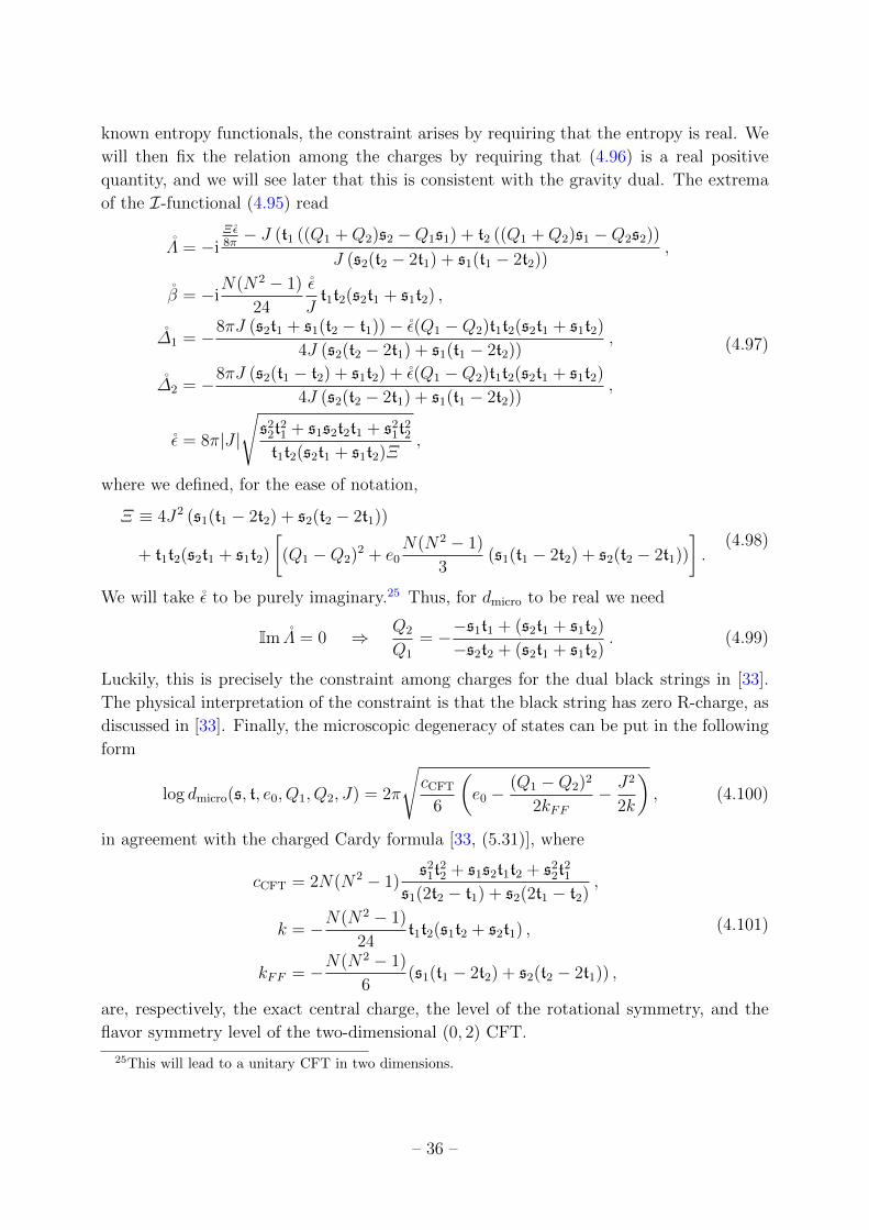
known entropy functionals, the constraint arises by requiring that the entropy is real. We
will then fix the relation among the charges by requiring that (4.96) is a real positive
quantity, and we will see later that this is consistent with the gravity dual. The extrema
of the I-functional (4.95) read
Λ = −iΞε8π− J (t1 ((Q1 +Q2)s2 −Q1s1) + t2 ((Q1 +Q2)s1 −Q2s2))
J (s2(t2 − 2t1) + s1(t1 − 2t2)),
β = −iN(N2 − 1)
24
ε
Jt1t2(s2t1 + s1t2) ,
∆1 = −8πJ (s2t1 + s1(t2 − t1))− ε(Q1 −Q2)t1t2(s2t1 + s1t2)
4J (s2(t2 − 2t1) + s1(t1 − 2t2)),
∆2 = −8πJ (s2(t1 − t2) + s1t2) + ε(Q1 −Q2)t1t2(s2t1 + s1t2)
4J (s2(t2 − 2t1) + s1(t1 − 2t2)),
ε = 8π|J |
√s2
2t21 + s1s2t2t1 + s2
1t22
t1t2(s2t1 + s1t2)Ξ,
(4.97)
where we defined, for the ease of notation,
Ξ ≡ 4J2 (s1(t1 − 2t2) + s2(t2 − 2t1))
+ t1t2(s2t1 + s1t2)
[(Q1 −Q2)2 + e0
N(N2 − 1)
3(s1(t1 − 2t2) + s2(t2 − 2t1))
].
(4.98)
We will take ε to be purely imaginary.25 Thus, for dmicro to be real we need
Im Λ = 0 ⇒ Q2
Q1
= −−s1t1 + (s2t1 + s1t2)
−s2t2 + (s2t1 + s1t2). (4.99)
Luckily, this is precisely the constraint among charges for the dual black strings in [33].
The physical interpretation of the constraint is that the black string has zero R-charge, as
discussed in [33]. Finally, the microscopic degeneracy of states can be put in the following
form
log dmicro(s, t, e0, Q1, Q2, J) = 2π
√cCFT
6
(e0 −
(Q1 −Q2)2
2kFF− J2
2k
), (4.100)
in agreement with the charged Cardy formula [33, (5.31)], where
cCFT = 2N(N2 − 1)s2
1t22 + s1s2t1t2 + s2
2t21
s1(2t2 − t1) + s2(2t1 − t2),
k = −N(N2 − 1)
24t1t2(s1t2 + s2t1) ,
kFF = −N(N2 − 1)
6(s1(t1 − 2t2) + s2(t2 − 2t1)) ,
(4.101)
are, respectively, the exact central charge, the level of the rotational symmetry, and the
flavor symmetry level of the two-dimensional (0, 2) CFT.
25This will lead to a unitary CFT in two dimensions.
– 36 –
5 A mixed index on (S2ε × S1)×Σg
The mixed index on (S2ε × S1) × Σg was first written down in [24] by gluing Nekrasov’s
partition functions. In this section, we describe the supersymmetric background for the
CFT partition function, and we recover the result using supersymmetric localization. We
begin by describing the rigid 5d N = 1 supergravity background, with topology S2×S1×Σg, on which the CFT lives. The metric on S2 × S1 will be such that the S2 is metrically
fibered over the S1, corresponding to angular momentum. The background is the same as
the 3d background which can be used to compute the three-dimensional superconformal
index. We will use a topological twist on Σg, so that the metric on Σg is irrelevant, except
for g = 0 where another angular momentum can be introduced when the metric admits a
continuous isometry. After reduction on the time circle, this type of angular momentum
is equivalent to an Ω-background. Our metric, spinor, and supergravity conventions are
mostly as in [23]. Spinor conventions are collected in appendix C.1, and supersymmetry
conventions in appendix C.2. Note that all of the spacetimes we consider are spin, and we
therefore do not need to introduce SpinC bundles.
The gravity side of the holography, in the case under consideration, consists of black
hole solutions of 6d matter coupled F (4) gauged supergravity. The ordinary F (4) gauged
supergravity, introduced by Romans in [71], was considered in the context of holography in
[72]. Therein, the boundary supergravity, which is coupled to a 5d N = 1 superconformal
theory, can be described using the ordinary Weyl multiplet of 5d superconformal tensor
calculus [73–76], described for instance in [77]. There are hardly any remnants, on the
boundary, of the complexities of the transformations in Romans supergravity. According
to [72], we can identify the boundary metric, SU(2)R gauge field, and antisymmetric tensor
directly with asymptotic values of the bulk supergravity. These are the fields which are
turned on for the simplest black hole solutions. More complicated solutions come from the
matter coupled supergravity. The boundary theory in that case is coupled to the Weyl
multiplet plus additional background vector multiplets. The conditions for preserving
supersymmetry in the boundary CFT are best derived by looking at the Weyl multiplet
first, and adding the matter multiplets on top.
5.1 Rigid supergravity background
A rigid bosonic supersymmetric background is a fixed point of the supersymmetry transfor-
mation of the Weyl multiplet [78–80]. We will follow the description of the Weyl multiplet
given in [77], translated into the notation of [23] using appendix C.2. The relevant super-
gravity fields are the vielbein eµa, the antisymmetric tensor Tab, and an SU(2) R-symmetry
gauge field A(R)µ .26
26The backgrounds we consider are very similar to those discussed in [81] in the context of four-
dimensional N = 2 supergravity. It seems likely that the background in [81] can be uplifted, and that the
analysis can be carried over to the five-dimensional case, although we were not able to verify this.
– 37 –

The supersymmetry transformation of the gravitino in the Weyl multiplet reads
δψµ = Dµξ +i
4Tab(3γabγµ − γµγab
)ξ − γµξ , (5.1)
where
Dµξ ≡ ∂µξ +1
4ωµ
abγabξ + ξ(A(R)µ
)T. (5.2)
Note thati
4Tνρ (3γνργµ − γµγνρ) =
i
2Tνρ (γµ
νρ − 4δµνγρ) , (5.3)
so that the antisymmetric tensor field of [72] can be identified with the one used in our
Weyl multiplet as
Bµν = −1
2Tµν . (5.4)
The identification of the other fields is equally straightforward.
We will describe in detail a solution to the equation δψµ = 0 corresponding to a
manifold with topology (S2 × S1) × S2, where a topological twist will be applied to the
second S2 factor. The solution is simple to derive by considering an ansatz whereby the
Killing spinor is the product of the ones for the 3d superconformal index, and a constant
spinor on the twisted S2. More general manifolds, with topology (S2×S1)×Σg for g ≥ 1,
can be included by simply changing the factor sin η in the metric, see (5.5), to 1, in the
case of g = 1, or to sinh η in the case of g ≥ 2. When g = 1, Σg is a torus, i.e. a quotient
of R2, and the supergravity fields and equations are independent of its coordinates. When
g ≥ 2, the Riemann surface Σg is a quotient of the hyperbolic plane, and we can solve the
gravitino equations by considering those on (S2 × S1) × H2 and noting that the Killing
spinor is independent of the coordinates of H2. The definition of the twisted fields, and
other aspects of localization considered below, are mostly independent of g. However, when
considering a compact Σg with g ≥ 1, one should turn off the Ω-deformation parameter
ε2, since such a manifold does not admit a continuous isometry with fixed points.
The background for g = 0. We choose the following vielbein on (S2θ,φ × S1
τ )× S2η,ϕ
e1 = rdθ , e2 = r sin θ (dφ− βε1dτ) , e5 = βdτ ,
e3 = r2dη , e4 = r2 sin η (dϕ− βε2dτ) .(5.5)
The real geometric parameters ε1,2 correspond to the real part of the angular momentum
fugacities when the partition function on this background is viewed as an index. We also
take an R-symmetry connection
A(R) = (−βε1dτ + cos η (βε2dτ − dϕ)) τ3 , (5.6)
corresponding to a partial twist on both the sphere and the part of the spin connection
related to the angular momentum on the twisted sphere, proportional to ε2. Lastly, we
turn on the antisymmetric tensor field T
T12 =1
6r. (5.7)
– 38 –

Observe that T is covariantly constant.
One may check that the Killing spinor equation δψµ = 0, see (5.1), is satisfied for ξ of
the form described below, and that the vanishing of the variation of the dilatino is likewise
guaranteed as long as one sets the supergravity field D to the value27
D =1
6r2+
1
16r22
. (5.8)
This background actually preserves 2 supercharges of the type covered by our ansatz.
In the limit ε1 → 0, the number of supercharges is further enhanced to 4. The same is
true for g ≥ 2 with the appropriate change of vielbein and with ε2 → 0. For g = 1, the
amount of supersymmetry is double that of g 6= 1 in every scenario.
The superalgebra. We choose a specific Killing spinor, which in the notation of ap-
pendix C.1 takes the form28
ξ =1
2
0 ie
iφ2 sin θ
2
−ie−iφ2 sin θ
20
e−iφ2 cos θ
20
0 eiφ2 cos θ
2
. (5.9)
We define δ to be the supersymmetry transformation associated with ξ. The superalgebra
generated by δ contains a number of bosonic transformations:
1. An infinitesimal diffeomorphism with parameter iv, where
v ≡ 1
β∂τ +
(ε1 +
i
r
)∂φ + ε2∂ϕ . (5.10)
2. An infinitesimal R-symmetry transformation given by the matrix
Λ = −1
2
(ε1 +
i
r
)σ3 , (5.11)
such that ξ transforms as
ξ → ξΛT . (5.12)
3. A gauge transformation which depends on the field realization.
One can explicitly check that there is no Weyl transformation, nor conformal isometries,
present in the square of the supersymmetry preserved on this background. This is a
necessary, but not sufficient, condition for using localization.
Note that the condition (C.14) cannot be solved for the pair ξ, ξ, hence the background
considered here is not reachable from the gauge fixed supergravity used in [82–85]. For
continuity with [23], we will nevertheless continue to use the notation from [82] for the
matter fields.27For g > 1 one should change the sign of the second term, while for g = 1 the second term is absent.28Note that ξ does not satisfy the symplectic Majorana reality condition (C.9). This is reminiscent of
the situation for the 3d superconformal index.
– 39 –

5.2 Localization
We would like to perform localization for an arbitrary N = 1 theory on the background
described above. We will describe first the moduli space arising from such localization.
This space is by definition the vanishing locus for the supersymmetry transformations of
all the fermions in the theory. However, the fields living in hypermultiplets, assuming that
they have generic masses coming from background flavor multiplets, will not contribute
any moduli. We therefore examine here the moduli coming from the vector multiplets,
which are the configurations for which the transformation of the gaugino vanishes.
The supersymmetry transformation of the gaugino reads
δλI = −1
2Γmn (Fmn − 4σTmn) ξI − iDmσΓ
mξI − iDIJξJ − 2iσξI . (5.13)
One can show that the following configuration solves the BPS equation δλ = 0
F (0) =n
2
(1
r2Vol(S2) + βε1 sin θdθ ∧ dτ
)+
m
2
(1
r22
Vol(Σg) + βε2 sin ηdη ∧ dτ
),
σ(0) =n
2r, D
(0)12 =
m
2r22
,(5.14)
where m and n are constants taking values in the magnetic weight lattice of G. They
correspond to fluxes for dynamical or background gauge fields. The BPS configuration
also implicitly includes a flat G connection commuting with m and n which, given the
topology of the space, can be taken to be a spacetime independent profile for Aτ .29 For
generic m, n, this flat connection is in the same Cartan subalgebra as m and n .
We henceforth work with the Cartan subalgebra defined by the above BPS config-
urations. These define the Coulomb branch of BPS pseudo-vacua. Due to large gauge
transformations wrapping the time circle, the Cartan elements of the flat connection, de-
noted by aflati , are compact
aflati ∼ aflat
i +2π
βn , n ∈ Z . (5.15)
Note also, that unlike the situation in [23] the Cartan elements of σ(0) are fixed by the
value of the fluxes, and do not define a separate non-compact direction of the Coulomb
branch moduli space.
The BPS configurations include D12 ∝ m, and therefore do not satisfy the original
reality conditions for the field DIJ . Instead, convergence of the path integral with a mea-
sure defined by the classical action of the gauge theory sets D12 to be purely imaginary,
or at least to have a bounded real part, if one makes the standard rotation from Lorentz
29When g ≥ 1, there exist additional factors of the moduli space of flat connections coming from the
holonomy on the non-contractible cycles of Σg. These do not appear as deformations of the superalgebra
and play no role in localization.
– 40 –

signature [23]. Configurations with auxiliary fields not satisfying the original reality condi-
tions are common in solutions to the BPS equations of twisted gauge theories [14, 23, 64].
One can try to explain their appearance by considering a δ-exact mixing term between an
auxiliary field and a dynamical scalar. Adding this term, and integrating over the orig-
inal contour, effectively sets the auxiliary field to a complex value in the BPS equation.
The need to add such a mixing term, in the context of localization, is usually attributed
to the existence of fermionic zero modes [86], or more generally to the need to lift some
of the moduli [87]. In some cases, they can also be understood from the point of view
of the effective low energy theory [88], where they represent a breakdown of localization
associated with contributions from the boundary of field space. We do not have a good
understanding of the arguments for the necessity of including these configurations as they
apply to the situation at hand. However, the consistency of the calculation implies that
they should be included.
5.2.1 Twisted fields
To examine the moduli space more closely, and to deduce the one loop exact effective
action, it is convenient to define twisted fields. Our definition of these fields is very similar
to the one given in [85], although the non-pseudo-Majorana nature of our Killing spinor
prevents us from using the expressions in that work directly.
Vector multiplets. We first define the spinor bilinears
κa ≡ ξγaξ , s ≡ ξξ . (5.16)
Note that the scalar s vanishes on a great circle in the untwisted S2, the equator with
respect to the fixed points of v, that κaκa = s2, and that at the poles s = ±1 and κa = δa5.
The vanishing of s means that the localization here is not of the type examined in [85] or
in [23].
We define the following operators acting on a 2-form Ξ
ΞV ≡ κ ∧ iκΞ , ΞH ≡ Ξ − ΞV ,
Ξ± ≡1
2
(ΞH ±
1
2siκ ? ΞH
).
(5.17)
Note that
Ξ = ΞV + Ξ+ + Ξ− , (5.18)
but that the decomposition is a complex one.
We now define the following twisted fields
Ψa ≡ ξIγaλI , χab ≡ sξIγabλ
I − (κaΨb − κbΨa) , Φ ≡ sσ − iiκA , (5.19)
and the auxiliary field
Hab ≡ 2s2F−ab +(s2 − 1
)FV ab + 2sξIγabξJD
IJ + 6si ¯ξIγabξIσ + iσ (κ ∧ ds)ab . (5.20)
– 41 –

One can show that the change of variables from λ to Ψa and χab is nonsingular, even at
the equator. One can also verify that the following projections hold
χV = χ+ = 0 , HV = H+ = 0 . (5.21)
There is a perhaps more natural change of variables, and definition of (anti)self-duality, for
the fermions which makes χ horizontal only at the poles and also either self-dual or anti-
self dual depending on which pole. In the end, it makes no difference for the localization
computation.
After the change of variables, we get the following supersymmetry transformations for
the twisted fields
δA = iΨ , δΨ = iκF − iD (sσ) = LκA− iDΦ ,
δχ = H , δH = Lκχ+ i [Φ, χ] , δΦ = 0 .(5.22)
We can compare these expressions to the ones for either the twisted backgrounds of [23],
or the contact type backgrounds of [85]. The only difference is the appearance of powers
of s. Had s been not just nowhere vanishing but actually constant, as was the case for
both [23] and [85], we would recover the full set of twisted fields defined in those papers.30
As in [23], we define
a ≡ −iΦ(0) = aflat . (5.23)
Hypermultiplets. The off-shell closed hypermultiplet introduced in appendix C.2 can
be twisted in the same manner as the vector multiplet. We define
q ≡ ξIqI , ψq ≡ −iδq , ψF ≡ PFψ , F ≡ δψF . (5.24)
The operator PF is a Hermitian spin projector which selects half of the components of the
spinor ψ. It is chosen so as to have rank 2, to annihilate ξI
PF ξI = 0 , for I = 1, 2 , (5.25)
and to be invariant under δ2, i.e.
LκPF = 0 .
The precise form of PF then determines the spinor F in terms of F I and some expression
linear in qI . In our chosen coordinates and vielbein, we can take
(PF )βα =
1
2
1− s 0 0 i
√1− s2
0 1− s −i√
1− s2 0
0 i√
1− s2 1 + s 0
−i√
1− s2 0 0 1 + s
. (5.26)
30Note that ξ, which is related to the field tIJ of [85], vanishes for the twisted backgrounds of [23].
– 42 –
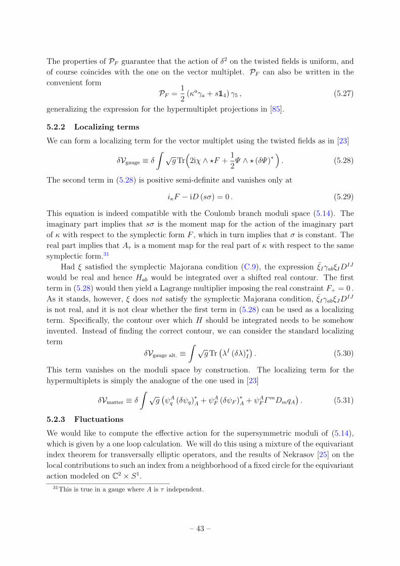
The properties of PF guarantee that the action of δ2 on the twisted fields is uniform, and
of course coincides with the one on the vector multiplet. PF can also be written in the
convenient form
PF =1
2(κaγa + s14) γ5 , (5.27)
generalizing the expression for the hypermultiplet projections in [85].
5.2.2 Localizing terms
We can form a localizing term for the vector multiplet using the twisted fields as in [23]
δVgauge ≡ δ
∫√gTr
(2iχ ∧ ?F +
1
2Ψ ∧ ? (δΨ)∗
). (5.28)
The second term in (5.28) is positive semi-definite and vanishes only at
iκF − iD (sσ) = 0 . (5.29)
This equation is indeed compatible with the Coulomb branch moduli space (5.14). The
imaginary part implies that sσ is the moment map for the action of the imaginary part
of κ with respect to the symplectic form F , which in turn implies that σ is constant. The
real part implies that Aτ is a moment map for the real part of κ with respect to the same
symplectic form.31
Had ξ satisfied the symplectic Majorana condition (C.9), the expression ξIγabξIDIJ
would be real and hence Hab would be integrated over a shifted real contour. The first
term in (5.28) would then yield a Lagrange multiplier imposing the real constraint F+ = 0 .
As it stands, however, ξ does not satisfy the symplectic Majorana condition, ξIγabξJDIJ
is not real, and it is not clear whether the first term in (5.28) can be used as a localizing
term. Specifically, the contour over which H should be integrated needs to be somehow
invented. Instead of finding the correct contour, we can consider the standard localizing
term
δVgauge alt. ≡∫√gTr
(λI (δλ)∗I
). (5.30)
This term vanishes on the moduli space by construction. The localizing term for the
hypermultiplets is simply the analogue of the one used in [23]
δVmatter ≡ δ
∫√g(ψAq (δψq)
∗A + ψAF (δψF )∗A + ψAFΓ
mDmqA). (5.31)
5.2.3 Fluctuations
We would like to compute the effective action for the supersymmetric moduli of (5.14),
which is given by a one loop calculation. We will do this using a mixture of the equivariant
index theorem for transversally elliptic operators, and the results of Nekrasov [25] on the
local contributions to such an index from a neighborhood of a fixed circle for the equivariant
action modeled on C2 × S1.
31This is true in a gauge where A is τ independent.
– 43 –

Vector multiplets. We will use the standard background gauge
D(0)µ aµ = 0 , (5.32)
where D(0)µ is the covariant derivative with respect to a background connection leading to
(5.14). Specifically, it is a connection which itself satisfies the gauge condition ∇µa(0)µ = 0 .
Such a representative is guaranteed to exist. We fix the gauge by adding a term to the
action given by
δBRST
∫√g cD(0)
µ aµ . (5.33)
We would like to verify that the relevant operator coming from V is transversally
elliptic. According to [89, 90], the relevant operator is Doe ⊂ V , which is defined as
the order zero term acting between the fields ϕe and ϕo. In our case ϕe = aµ, while
ϕo = χ, c, c, where c, c are the ghost and anti-ghost in the gauge fixing multiplet [89].
We find Doe by expressing λ in V as the unique linear combination of χ and Ψ derived
above. We then expand V around the forms in the non-coordinate basis: aa, χab, c, c. We
denote the corresponding momenta by pa. We find that the (leading) matrix symbol of
Doe is given by32
− p42s2
p32s
−p22s
p12s2
0
− p32s2
−p42s
p12s2
p22s
0
− p22s2
p12s2
p42s3
− p32s3
0p42s3
− p32s2
p22s2
− p12s3
0
− p32s3
− p42s2
p12s3
p22s2
0p22s
−p12s− p4
2s2p32s2
0
−p1p5 −p2p5 −p3p5 −p4p5 p21 + p2
2 + p23 + p2
4
p1 p2 p3 p4 p5
. (5.34)
The top 6 rows correspond to χab, row 7 to c, and row 8 to c. One can clearly see that
the rows 4, 5, 6 are multiples of the rows 1, 2, 3. This is the reflection of the fact that
χab is actually constrained, and has only 3 degrees of freedom. We choose to remove the
rows 4, 5, 6, and to call the remaining 5 × 5 matrix the matrix symbol of Doe, denoted
σ (Doe). We can now evaluate the determinant of σ (Doe). It is given by
detσ (Doe) = − 1
8s6~p 2(~p 2 − p2
5
) (p2
1 + p23 + p2
4 + s2p22
). (5.35)
Note that the singular factor of s−6 is an artifact of the coordinate system and our definition
of the twisted fermions and plays no physical role.
32We have ignored various numerical constants which multiply entire rows or columns, since these do
not affect the invertibility of the symbol.
– 44 –
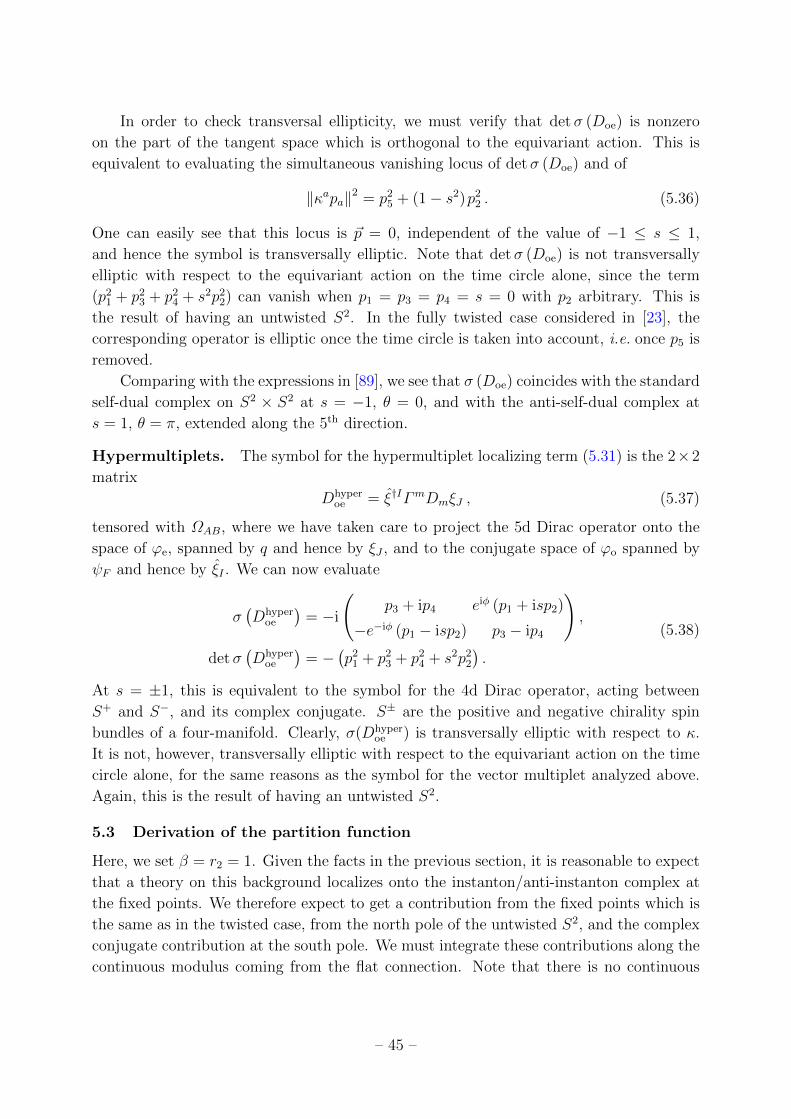
In order to check transversal ellipticity, we must verify that detσ (Doe) is nonzero
on the part of the tangent space which is orthogonal to the equivariant action. This is
equivalent to evaluating the simultaneous vanishing locus of detσ (Doe) and of
‖κapa‖2 = p25 + (1− s2)p2
2 . (5.36)
One can easily see that this locus is ~p = 0, independent of the value of −1 ≤ s ≤ 1,
and hence the symbol is transversally elliptic. Note that detσ (Doe) is not transversally
elliptic with respect to the equivariant action on the time circle alone, since the term
(p21 + p2
3 + p24 + s2p2
2) can vanish when p1 = p3 = p4 = s = 0 with p2 arbitrary. This is
the result of having an untwisted S2. In the fully twisted case considered in [23], the
corresponding operator is elliptic once the time circle is taken into account, i.e. once p5 is
removed.
Comparing with the expressions in [89], we see that σ (Doe) coincides with the standard
self-dual complex on S2 × S2 at s = −1, θ = 0, and with the anti-self-dual complex at
s = 1, θ = π, extended along the 5th direction.
Hypermultiplets. The symbol for the hypermultiplet localizing term (5.31) is the 2×2
matrix
Dhyperoe = ξ†IΓmDmξJ , (5.37)
tensored with ΩAB, where we have taken care to project the 5d Dirac operator onto the
space of ϕe, spanned by q and hence by ξJ , and to the conjugate space of ϕo spanned by
ψF and hence by ξI . We can now evaluate
σ(Dhyper
oe
)= −i
(p3 + ip4 eiφ (p1 + isp2)
−e−iφ (p1 − isp2) p3 − ip4
),
detσ(Dhyper
oe
)= −
(p2
1 + p23 + p2
4 + s2p22
).
(5.38)
At s = ±1, this is equivalent to the symbol for the 4d Dirac operator, acting between
S+ and S−, and its complex conjugate. S± are the positive and negative chirality spin
bundles of a four-manifold. Clearly, σ(Dhyperoe ) is transversally elliptic with respect to κ.
It is not, however, transversally elliptic with respect to the equivariant action on the time
circle alone, for the same reasons as the symbol for the vector multiplet analyzed above.
Again, this is the result of having an untwisted S2.
5.3 Derivation of the partition function
Here, we set β = r2 = 1. Given the facts in the previous section, it is reasonable to expect
that a theory on this background localizes onto the instanton/anti-instanton complex at
the fixed points. We therefore expect to get a contribution from the fixed points which is
the same as in the twisted case, from the north pole of the untwisted S2, and the complex
conjugate contribution at the south pole. We must integrate these contributions along the
continuous modulus coming from the flat connection. Note that there is no continuous
– 45 –

modulus coming from the vev of σ, since this is fixed by the moment map equation (5.29).
The modulus a is therefore integrated over a shifted real contour. We must also sum over
the localized instantons/anti-instantons and over the two sets of fluxes m, n.
When evaluating the partition function on our spaces, using either Nekrasov’s instan-
ton partition function or the equivariant index theorem, the effective values of the real
part of the angular momentum parameters at the north and south poles of the untwisted
two-sphere have a relative minus sign.33 Define the following complex angular momentum
parameter
εN/S1 = ε
N/S1 − sN/S i
r, (5.39)
where εN/S1 is the plus or minus real geometric parameter ε1, and sN/S takes the values ∓1
when the point in question is localized at the north and south poles of the untwisted sphere,
respectively. The linear combinations εN/S1 are all that ever appear in the calculation,
whether as parameters of the equivariant action, or as coefficients multiplying the flux n.
We henceforth work only with this combination, and denote
ε1 ≡ ε1 +i
r. (5.40)
There is no analogous shift for ε2, which we now rename to ε2.
For the case of g = 0, we can simply make use of the 5d Nekrasov partition function
to compute the partition function. The conjecture in [8] implies that the full result can
be written as a sum over equivariant fluxes and an integral over a of 4 copies of the 5d
Nekrasov partition function associated to the 4 fixed points. We have derived the fact that
the partition function actually depends on only two fluxes: m, n which correspond to the
homology two cycles of the spacetime manifold. We therefore write the result as
Z(S2ε1×S1)×S2
ε2=∑m,n
∮da
4∏l=1
ZC2×S1
(a(l); ε
(l)1 , ε
(l)2
). (5.41)
We choose a parametrization of these fluxes which is suited to the present context. In this
parametrization, the parameters a(l) in the fully twisted case would be given by34
a(l) = a− ε(l)1
n
2+ ε
(l)2
m
2.
The fixed point data is given in table table 2.35 The points 1, 2 lie at the north pole of the
untwisted sphere, and 3, 4 at the south pole.
33ε1 is the coefficient of the rotation with respect to φ, which rotates the local frame at the north and
south poles in opposite directions.34The factors of 1/2 have been inserted in order to match the quantization conditions on m, n with the
expression given in terms of the parameters pl (cf. [23, Sect. 2.7.2]).35The fixed point data given in [23] is adapted to a general toric geometry. We prefer to use a simpler
table for the specific manifold considered here.
– 46 –

l 1 2 3 4
ε(l)1 ε1 ε1 −ε1 −ε1ε
(l)2 ε2 −ε2 ε2 −ε2
Table 2: Values of the equivariant parameters for S2ε1× S2
ε2.
The perturbative part of the Nekrasov partition function can be calculated using
the equivariant index theorem for transversally elliptic operators. There is an important
subtlety in using the equivariant index theorem in the situation where the symbol is only
transversally elliptic and not elliptic. One must be careful about how to expand the
infinite sum in the index in order to translate it into a determinant [89]. A derivation
for the specific case of the superconformal index was performed in [91]. The prescription
used in [91], which recovers the result for the superconformal index computed by counting
operators, is that half of the effective a(l), associated to the south pole of the sphere, should
be multiplied by an overall −1 (cf. [91, (5.15)-(5.17)]). Adopting this approach, we change
the sign of a and ε(l)1 for points at the south pole, corresponding in our case to points 3, 4.
From the point of view of the full Nekrasov partition function, this prescription presumably
coincides with what one gets by including anti-instantons instead of instantons at one of
the poles. We have already seen that the symbols for the fluctuation operators imply that
this should be the case.
The relevant parameters are therefore
a(l) = a− ε(l)1
n
2+ ε
(l)2
m
2, north pole of S2
ε1,
a(l) = −a+ ε(l)1
n
2+ ε
(l)2
m
2, south pole of S2
ε1.
(5.42)
Taking the data from table 2, we get the following set of parameters
a(1) = a− ε1n
2+ ε2
m
2,
a(2) = a− ε1n
2− ε2
m
2,
a(3) = −a− ε1n
2+ ε2
m
2,
a(4) = −a− ε1n
2− ε2
m
2.
(5.43)
For hypermultiplets, we can introduce background holonomies corresponding to fu-
gacities ∆. In addition to the overall sign change noted above, there is a shift of the origin
of ∆ [23]. This shift was first discussed in [92]. The relevant shift in the purely twisted
case was a uniform shift, which with our conventions for εi is
∆→ ∆− 1
2
(ε
(l)1 − ε
(l)2
). (5.44)
– 47 –

In the case at hand, where the sign of ∆, like that of a, changes between the north and
south poles, it is better to think of the shift as a shift of the overall parameter. Combining
with the result for the vectors, we get the following
∆(l) = ∆− 1
2
(ε
(l)1 + ε
(l)2
)− ε(l)1
t
2+ ε
(l)2
s
2, north pole of S2
ε1,
∆(l) = −∆− 1
2
(ε
(l)1 + ε
(l)2
)+ ε
(l)1
t
2+ ε
(l)2
s
2, south pole of S2
ε1.
(5.45)
In standard conventions, the origin of flavor fluxes s, t would also be at 0. However,
we use conventions in which the background fluxes for the universal twist are at s = 1−g.
For g = 0 we therefore take s below to be the flavor flux on the twisted sphere plus one.
Taking the data from table 2, we get the following set of parameters
∆(1) = ∆− ε1t + 1
2+ ε2
s− 2
2,
∆(2) = ∆− ε1t + 1
2− ε2
s− 2
2,
∆(3) = −∆− ε1t− 1
2+ ε2
s− 2
2,
∆(4) = −∆− ε1t− 1
2− ε2
s− 2
2.
(5.46)
For the cases g ≥ 1 one does not have isolated fixed points. Instead, the fixed loci of
the action of v are copies of Σg. The partition function on these spaces can be computed
from the two different perspectives, leading to the same result. We consider the situation
with g arbitrary and therefore set ε2 to 0.
5.3.1 The perturbative partition function
We are interested primarily in determining the partition function in the large N limit,
hence we assume that we can safely ignore non-perturbative contributions. The remaining
elements of the localization calculation are the classical and one loop pieces.
The classical piece. The classical action on the current background is different from
the one indicated in [23]. As in [23], the part of the action containing hypermultiplets will
not contribute a classical term because there are no moduli in this sector of the theory. A
superconformal action for vector multiplets was constructed in [76]. The action depends
on a totally symmetric tensor CABC and vector multiplets VA. In order to construct a
Yang-Mills-like action for a dynamical vector multiplet, one of the VA should be taken
to be a background abelian multiplet fixed to a supersymmetric configuration. Such a
configuration necessarily breaks conformal symmetry.36 For the time being, we reinstate
β, r, r2.
36One may also construct topological Chern-Simons terms which preserve conformal symmetry.
– 48 –

The bosonic action for abelian VA, translated into our field variables and with an
overall normalization which matches that of [23], is given by [76]
S =
∫√g CABC Tr
[σA(
1
2FBµνF
µνC +DµσBDµσC +
1
2DIJ,ADB
IJ − 6σBFCµνT
µν
)
− i
12εµνρστAAµF
BνρF
Cνρ + σAσBσC
(− 1
12R +
8
3D + 13TµνT
µν
)].
(5.47)
We will choose the index A to run from 1 to 2, with V2 the dynamical vector multiplet
and V1 a background vector multiplet. We also choose the following symmetric tensor
CABC = CδA1δB
2δC2 + symmetrization . (5.48)
In order to get a Yang-Mills like term, we set the following background configuration for
V137
F 1 =1
2
[1
r2Vol(S2) + βε1 sin θdθ ∧ dτ
], σ1 =
1
2r, (5.49)
with all other fields vanishing. In order to get the normalization for the Yang-Mills term
used in [23], we will take C = 2r/g2YM.
It is now straightforward to evaluate the classical contribution to the partition func-
tion, by replacing both the supergravity fields and the dynamical vector multiplet fields
with their background values. The result is
Sclassical = −i16π2r
g2YM
Tr(ma) . (5.50)
There are various puzzling issues about this result. First, (5.50) is not holomorphic in
ε1 as we would expect from gluing the classical pieces of the Nekrasov partition function.
It actually coincides with the result of the gluing when ε1 is purely imaginary (see section
5.3.2). It would be interesting to understand if there exist some extra terms in the bosonic
action that could reproduce a manifestly holomorphic result.
Secondly, note that due to the periodicity of a, see (5.15), the classical term is not
gauge invariant under large gauge transformations. This is already apparent at the level
of the 5d Nekrasov partition function. The issue did not come up in the fully twisted case,
described in [23], because the classical contributions had a different structure. There are
at least two possibilities to avoid this. For theories with 5d fixed points, gYM must be
taken to∞ before evaluating the partition function in order to flow to the conformal fixed
point. The calculation at intermediate values of gYM is presumably ill defined. For theories
with a 6d fixed point, on the other hand, it is not completely clear what six-dimensional
observable we are computing, and other details of the 6d physics might come to rescue.
37In order to preserve the appropriate supersymmetries, the background configurations are restricted
to the ones that yield the dynamical moduli.
– 49 –

Another possibility is that the classical part of the action is always ambiguous because,
as is the case for non-conformal theories in 4d, its coefficient can be changed by changing
the scale which is introduced in computing the one-loop contribution.
The one loop piece. It should be the case that the one loop determinant can be
constructed from the determinants used in the superconformal index, i.e. the partition
function on S2 × S1, raised to an appropriate power, which stems from the degeneracy of
zero energy modes on Σg. An explanation for this assertion is as follows. The one loop
contribution can be computed using the equivariant index theorem. In the situation at
hand, where the fixed loci with respect to the action of the symmetry generator are not
points but copies of Σg, the relevant index theorem is a hybrid of the equivariant index
theorem for the case of discrete fixed points, and the usual Atiyah-Singer index theorem
applied to the fixed loci. The two contributions should be multiplied to get the result on
the product space.38 This applies directly to the index for the twisted Dirac operator,
while the index for the AHS (instanton) deformation complex reduces to the twisted de
Rahm complex at the fixed loci. The result of the calculation with the AS index theorem
is simply a number, which we associate with the degeneracy. Hence, the result of the one
loop calculation is the one stemming from the equivariant index theorem on S2×S1, raised
to the power of the degeneracy.
The relevant fluctuation operators for computing the degeneracy can be easily ex-
tracted by evaluating the symbols σ (Doe) and σ(Dhyperoe ) near the fixed points of the
untwisted sphere and restricting to momenta along the twisted directions only. The de-
generacy can then be computed using the ordinary index theorem for the relevant complex.
For a line bundle of degree d on a Riemann surface of genus g, the Atiyah-Singer index
theorem yields d+ 1− g for the twisted Dolbeault complex, which controls the hypermul-
tiplets. A hypermultiplet valued in a weight ρ of the dynamical gauge group and a weight
ν of the flavor symmetry group therefore has degeneracy (cf. [14])
− ρ(m)− ν(s) + g− 1 . (5.51)
The overall minus sign comes from the opposite grading of the Dirac and Dolbeault com-
plexes. The origin for the flavor fluxes is at 2g− 2, and the shifted expression is
− ρ(m)− ν(s)− g + 1 . (5.52)
The vector multiplet is controlled by a twisted version of the de Rahm complex, which
is again related to the Dolbeault complex and yields the same result (c.f. [14]). The
degeneracy for a mode proportional to a root α reads
α (m) + 1− g . (5.53)
38The validity of these assertions is most apparent in the delocalized approach of Berline and Vergne
to the equivariant index theorem, where the index is calculated using an integral over equivariant charac-
teristic classes [93].
– 50 –
We must also specify the R-charge of the chirals appearing in the superconformal
index. To do this, we compare the square of the supercharge used to localized the SCI
with th eone used here. The ratio of the ε1 dependent term between the derivative with
respect to φ and the R-symmetry transformation acting on q1 is −2. In the context of the
SCI, where the eigenvalue with respect to said derivative is usually denoted j3, the ratio
is −2/∆, where ∆ is both the R-charge and the Weyl weight of the bottom component
of a chiral superfield (cf. [91, (5.14)]). Evidently, we should set ∆ to 1. Vector multiplets
can also be treated as chiral multiplets for the purposes of constructing the partition
function. This is because a chiral multiplet of R-charge 0 can get a vev and Higgs a vector
multiplet, yielding an empty theory in the IR. It also holds that the product of the one
loop determinants of chiral multiplets with R-charges ∆ and 2 − ∆ is 1 [94]. the vector
multiplet may therefore be treated as a chiral multiplet with R-charge 2.
Fermionic zero modes. One must still deal with the fermion zero modes which are the
superpartners of the holonomies on Σg. This can presumably be done using the approach
described in e.g. [64], but the details are more complicated in the 5d context. We will rely
on the 2d result.
5.3.2 The final formula
We are ready to write the partition function. The result was first derived in [24] by gluing
Nekrasov partition functions. We set
ε1 = ε , ε2 = 0 , (5.54)
in the following. As already mentioned, in our conventions for the background fluxes, the
universal twist [29] corresponds to s = 1− g. One could also set the background fluxes on
the untwisted two-sphere to zero, t = 0, however, it is vital to keep ε nonzero. Finally, we
define
BρI ≡ ρI(m) + νI(s) + g− 1 , Bα ≡ α(m)− g + 1 . (5.55)
The mixed index can be written as [24]
Z(m, n, a; s, t, ∆, ε) =1
|W |∑
m,n∈Γh
∮C
rk(G)∏i=1
dxi2πixi
(detij
∂2W(S2ε×S1)×R2(a, n;∆, t, ε)
∂ai∂aj
)g
× exp
(16π2
g2YMε
TrF(ma)
)∏α∈G
[(x−αζ−α(n); ζ2)∞(xαζ2−α(n); ζ2)∞
(− ζxα
) 12α(n)]Bα
×∏I
∏ρI∈RI
[(xρIyνIζ1−ρI(n)−νI(t); ζ2)∞
(x−ρIy−νIζ1−ρI(n)−νI(t); ζ2)∞(−xρIyνI )−
12
(ρI(n)+νI(t))
]BρI,
(5.56)
with x = eia, y = ei∆, ζ = eiε/2, and W(S2ε×S1)×R2(a, n; ε) denoting the effective twisted
superpotential of the five-dimensional N = 1 theory on (S2ε × S1)×R2, whose expression
is the subject of the next section.
– 51 –

For g = 0, the partition function can be obtained by gluing the Nekrasov partition
function (4.15) using the rules discussed in section 5.3 and sending ε2 to zero [24]. The
appearance of the determinant of the effective twisted superpotential for g 6= 0 is dis-
cussed in section 5.4. As noticed in section 5.3.1, the one-loop contributions are obtained
by raising one-loop determinants of the partition function on S2ε × S1, the generalized
superconformal index, to integer powers, Bα and Bρ, counting the number of zero-modes
on the twisted Σg. The one-loop contribution of a chiral multiplet of R-charge rK to the
three-dimensional superconformal index reads [94, 95]
logZ∆K , tK , rKχ (a) =
(q
12
(1−rK)x−1y−1K
)− 12
(n+tK)
(x−1y−1
K q12
(2−rK−n−tK); q)∞(
xyKq12
(rK−n−tK); q)∞
, (5.57)
where yK = ei∆K and tK denote the flavor fugacity and magnetic flux, respectively. Setting
rK = 1 and yK = y, tK = t we recognize the contributions of the hypermultiplets in (5.56),
while setting rK = 2 and ∆K = 2π, tK = 0 we recognize the contributions of the vector
multiplets. Finally, the gluing procedure produces a classical term which is manifestly
holomorphic in ε1 and coincides with (5.50) when ε1 is purely imaginary. As already
discussed in section 5.3.1, the role of the classical term, which is not gauge invariant, is
not completely clear to us. In any event, it will only contribute to the partition function
of the N = 2 super Yang-Mills theory whose interpretation as a six-dimensional index has
yet to be clarified.
5.4 W(S2ε×S1)×R2 and its factorization
In this section we derive the effective twisted superpotential of the two-dimensional theory
obtained by compactifying a five-dimensional N = 1 theory on S2ε × S1.
(i) Gluing W(S2ε×S1)×R2. The two-sphere S2
ε is not twisted. We shall use the gluing
procedure that was detailed in section 4.1. For this purpose, we employ the identity gluing
that follows from the rules given in section 5.3 when ε2 = 0
a(1)k = ak −
ε
2nk , ∆(1) = ∆− ε
2(t + 1) , ε
(1)1 = ε ,
a(2)k = −ak −
ε
2nk , ∆(2) = −∆− ε
2(t− 1) , ε
(2)1 = −ε .
(5.58)
We can then write39
W(S2ε×S1)×R2(a, n;∆, t, ε) =W(R2
ε×S1)×R2(a(1);∆(1), ε(1))−W(R2ε×S1)×R2(a(2);∆(2), ε(2)) ,
(5.59)
where W(R2ε×S1)×R2 is given in (4.19)-(4.23).
39The relative minus follows from the relative minus for a in the identity gluing and the fact that Wappears with a derivative in the partition function, see (5.64).
– 52 –

Explicitly, the classical Yang-Mills contribution to the effective twisted superpotential
is given by
WYM(S2ε×S1)×R2(gYM, a, n; ε) = − 8iπ2
g2YMε
(TrF(a)2 +
ε2
4TrF(n)2
). (5.60)
Next, the contribution of a hypermultiplet to the twisted superpotential, in an expansion
around ε→ 0, reads
WH(S2ε×S1)×R2(a, n;∆, t, ε) = −
∑ρI∈R
∞∑s=0
(iε)s−1
(2π)sws (ρI(a), ρI(n); νI(∆), νI(t), 1) , (5.61)
where
ws(a, n;∆, t, r) ≡ gs (π(r − n− t)])
[Li3−s(e
i(a+∆)) +i3−s
2g3−s(a+∆)
]+ gs (π(2− r − n− t))
[Li3−s(e
−i(a+∆)) +i3−s
2g3−s(2π − a−∆)
],
(5.62)
with gs(a) defined in (4.5).40 Observe that gs(a) = 0 for s < 0. The contribution of a
vector multiplet is simply given by
WV(S2ε×S1)×R2(a, n; ε) =
∑α∈G
∞∑s=0
(iε)s−1
(2π)sws (α(a), α(n); 2π, 0, 2) . (5.63)
(ii) Bethe approach. Alternatively, the twisted superpotential appears in the mixed
index as41
Z(S2ε×S1)×Σg
=1
|W |∑
m,n∈Γh
∮C
rk(G)∏i=1
dxi2πixi
exp
(i
rk(G)∑k=1
mk
∂W(S2ε×S1)×R2(a, n; ε)
∂ak
)Zint
∣∣m=0
(a, n; ε) ,
(5.64)
where Zint is the integrand in (5.56), as a direct computation shows.
Performing the sum over the gauge magnetic fluxes m through the Riemann surface
in (5.64), we find a set of poles a at the Bethe vacua. It remains to evaluate the sum over
the gauge fluxes n on S2ε . At this stage, we assume that the mixed index localizes at the
solutions to the generalized BAEs
1 = exp
(∂W(S2
ε×S1)×R2(a, n; ε)
∂ak
)∣∣∣a=a, n=n
,
1 = exp
(∂W(S2
ε×S1)×R2(a, n; ε)
∂nk
)∣∣∣a=a, n=n
.
(5.65)
40Note that the sign of Re(a+∆) is opposite in the two terms in (5.59) and we need to shift accordingly
the functions gs(a) in (4.19)-(4.23).41We dropped the dependence on the flavor parameters (∆, s, t) to avoid clutter.
– 53 –

5.4.1 USp(2N) gauge theory with matter
We will now evaluate the effective twisted superpotential of the USp(2N) theory with
matter in the large N limit. The result will take a simple form using a democratic basis
for the flavor chemical potential ∆m and the fluxes (s, t)
s1 ≡ sm , s2 ≡ 2(1− g)− sm , s.t.2∑i=1
si = 2− 2g ,
t1 ≡ tm , t2 ≡ −tm , s.t.2∑i=1
ti = 0 ,
∆1 ≡ ∆m +ε
2, ∆2 ≡ 2π −∆m +
ε
2, s.t.
2∑i=1
∆i = 2π + ε .
(5.66)
The effective twisted superpotential has the same structure as (3.7) and we only need
to replace F∆k, tK (a), see (3.9), with
W∆K , tk, r(S2ε×S1)×R2(a) = −
∞∑s=0
(iε)s−1
(2π)sws(a, n;∆K , tK , r) , (5.67)
with ws(a, n;∆K , tK , r) given in (5.62). Let us start with the WA+V1(S2ε×S1)×R2 contribution.
Using (4.10), and assuming that | Im ai| → ∞, we obtain
WA+V1(S2ε×S1)×R2 = − 1
4ε
N∑i>j
[(4∆1∆2 + ε2t1t2)aij + ε2(∆1t2 +∆2t1)nij
]sign (Im aij)
− 1
4ε
N∑i>j
[(4∆1∆2 + ε2t1t2)a+
ij + ε2(∆1t2 +∆2t1)n+ij
]sign
(Im a+
ij
).
(5.68)
Assuming also that the eigenvalues are ordered by increasing imaginary part, i.e. ai > ajfor i > j, and using (3.13), we can simplify (5.68) further and write
WA+V1(S2ε×S1)×R2 = − 1
4ε
N∑k=1
(2k − 1)[(4∆1∆2 + ε2t1t2)ak + ε2(∆1t2 +∆2t1)nk
]. (5.69)
The contribution WF+V2(S2ε×S1)×R2 to the twisted superpotential at large N can be computed
similarly using (4.10) and it is given by
WF+V2(S2ε×S1)×R2 = −(8−Nf )
3ε
N∑k=1
(a2k +
3ε2
4n2k
)ak . (5.70)
– 54 –

Putting (5.69) and (5.70) together we obtain the final expression for the twisted superpo-
tential W(S2ε×S1)×R2 ,
W(S2ε×S1)×R2(a, n;∆, t, ε) = −(8−Nf )
3ε
N∑k=1
(a2k +
3ε2
4n2k
)ak
− 1
4ε
N∑k=1
(2k − 1)[(4∆1∆2 + ε2t1t2)ak + ε2(∆1t2 +∆2t1)nk
],
(5.71)
that can be recast in the following factorized form
W(S2ε×S1)×R2(a, n;∆, t, ε) = −2π
2∑σ=1
FSW
(a
(σ)k ;∆
(σ)i
)ε(σ)
, (5.72)
with FSW(ak;∆i) given in (4.44), using the identity gluing parameterization
a(1)k ≡ ak −
ε
2nk , ∆
(1)i ≡ ∆i −
ε
2ti , ε(1) = ε ,
a(2)k ≡ ak +
ε
2nk , ∆
(2)i ≡ ∆i +
ε
2ti , ε(2) = ε .
(5.73)
The Bethe solution can be obtained by extremizing (5.71) with respect to the gauge
variables (ak, nk). We find
∂W(S2ε×S1)×R2(a, n)
∂nk
∣∣∣nk=nk
= 0 ⇒ aknk = − (2k − 1)
2(8−Nf )(∆1t2 +∆2t1) , (5.74)
and
∂W(S2ε×S1)×R2(a, n)
∂ak= 0∣∣∣ak=ak, nk=nk
⇒ ak =i
2
√2k − 1
8−Nf
(√(∆1 +
ε
2t1
)(∆2 +
ε
2t2
)+
√(∆1 −
ε
2t1
)(∆2 −
ε
2t2
)).
(5.75)
Observe that (5.74) and (5.75) are equivalent to
∂FSW(a(σ)k ;∆
(σ)i )
∂a(σ)k
= 0 ⇒ a(σ)k =
i√8−Nf
√(2k − 1)∆
(σ)1 ∆
(σ)2 , (5.76)
for σ = 1, 2. Note that we use the determination 0 < ∆i ∓ ε2ti < 2π, i = 1, 2. Plugging
the saddle points (ak, nk) back into the twisted superpotential (5.71) we obtain
W(S2ε×S1)×R2(∆i, ti, ε) =
4π2i
27ε
[FS5
(∆i +
ε
2ti
)+ FS5
(∆i −
ε
2ti
)], (5.77)
with FS5(∆i) being, in form, the free energy of the theory on S5,
FS5(∆i) = −9√
2
5π2
N5/2√8−Nf
(∆1∆2)32 ,
2∑i=1
∆i = 2π + ε . (5.78)
– 55 –

5.4.2 N = 2 super Yang-Mills
ForN = 2 super Yang-Mills we find a dependence on the non-gauge invariant classical term
(5.50), whose interpretation is not clear. It is nevertheless instructive to check that the
twisted superpotential factorizes. Define the democratic basis for the chemical potential
∆i and the fluxes (si, ti), associated to the U(1)2 ⊂ SO(5) R-symmetry
s1 ≡ s , s2 ≡ 2(1− g)− s , s.t.2∑i=1
si = 2− 2g ,
t1 ≡ t , t2 ≡ −t , s.t.2∑i=1
ti = 0 ,
∆1 ≡ ∆+ε
2, ∆2 ≡ 2π −∆+
ε
2, s.t.
2∑i=1
∆i = 2π + ε .
(5.79)
The twisted superpotential of the theory reads
W(S2ε×S1)×R2 =WYM(ak, nk) +WH(ai, ni;∆, t, ε) +WV(ai, ni, ε) , (5.80)
with
WYM = − 8π2i
g2YMε
N∑k=1
(a2k +
ε2
4n2k
),
WH =N∑
i,j=1
W∆, t, r=1(aij) , WV = −N∑i 6=j
W∆=2π, t=0, r=2(aij) ,
(5.81)
and W∆, t, r(a) given in (5.67). In the strong ’t Hooft coupling λ 1, assuming that
| Im(ai − aj)| → ∞, (5.80) can be approximated as, using (4.10),
W(S2ε×S1)×R2(ai, ni;∆, t, ε) = − 8π2i
g2YMε
N∑k=1
(a2k +
ε2
4n2k
)
− 1
8ε
N∑i,j=1
[(4∆1∆2 + ε2t1t2)aij + ε2(∆1t2 +∆2t1)nij
]sign(Im aij) .
(5.82)
Assuming that the eigenvalues are ordered by increasing imaginary part, we can trade the∑Ni,j=1 with
∑Nk=1 using (3.13) to write
W(S2ε×S1)×R2(ai, ni;∆, t, ε) = − 8π2i
g2YMε
N∑k=1
(a2k +
ε2
4n2k
)
− 1
4ε
N∑k=1
(2k − 1−N)[(4∆1∆2 + ε2t1t2)ak + ε2(∆1t2 +∆2t1)nk
],
(5.83)
– 56 –

that, using the identity gluing parameterization (5.73), can be recast in the following
factorized form
W(S2ε×S1)×R2(a, n;∆, t, ε) = −2π
2∑σ=1
FSW
(a
(σ)k ;∆
(σ)i
)ε(σ)
, (5.84)
with FSW(ak;∆i) given in (4.61). We extremize (5.83) over the gauge variables (ak, nk) to
obtain the solution
ak = ig2
YM
64π2(2k − 1−N)(4∆1∆2 + ε2t1t2) ,
nk = ig2
YM
16π2(2k − 1−N)(∆1t2 +∆2t1) ,
(5.85)
to the generalized BAEs (5.65). Observe that (5.85) is equivalent to
∂FSW(a(σ)k ;∆
(σ)i )
∂a(σ)k
= 0 ⇒ a(σ)k = i
g2YM
16π2(2k − 1−N)∆
(σ)1 ∆
(σ)2 , (5.86)
for σ = 1, 2. Substituting these values into (5.83) we find
W(S2ε×S1)×R2(∆, t, ε) = − ig2
YM
3× 29π2ε
[(4∆1∆2 + ε2t1t2) + 2iε(∆1t2 +∆2t1)
]×[(4∆1∆2 + ε2t1t2)− 2iε(∆1t2 +∆2t1)
].
(5.87)
Remarkably, this can be recast in the following factorized form
W(S2ε×S1)×R2(∆, t, ε) = −iN(N2 − 1)
g2YM
192π2ε
[(∆
(1)1 ∆
(1)2
)2+(∆
(2)1 ∆
(2)2
)2]. (5.88)
5.5 Factorization of the index
In this section we will make the assumption that the mixed index localizes at the solutions
to the generalized BAEs (5.65). Given (5.64), up to subleading constant factors, the saddle
point contribution to the index is given by
Z(S2ε×S1)×Σg
= Zint
∣∣m=0
(a, n; ε)
∣∣∣∣n=n,a=a
. (5.89)
We will show that this expression factorizes,42 and leads to the correct entropy for a class
of dual black holes in massive type IIA. Moreover, as for the twisted index, we find
logZ(S2ε×S1)×Σg = i
2∑i=1
si∂W(S2
ε×S1)×R2
∂∆i
. (5.90)
While the mixed index for the Seiberg theory correctly reproduces the entropy of black
holes in massive type IIA, it is not clear what is the interpretation of the mixed index of
42Our results differ from those in [24], which do not factorize, due to a different twisted superpotential
used in the conjectured BAEs.
– 57 –

N = 2 super Yang-Mills in terms of the six-dimensional UV fixed point and we are not
aware of dual backgrounds where to test the large N result, which, as already mentioned,
explicitly depends on the existence of a non-gauge invariant classical term (5.50). It is
however interesting to observe that the result factorizes, as expected.
5.5.1 USp(2N) gauge theory with matter
We are interested in evaluating the mixed index (5.89) of the USp(2N) gauge theory in
the large N limit. To this aim, let us first consider the building block
Z(a,m, n;∆, s, t, ε) =
[(xyζr−n−t; ζ2)∞
(x−1y−1ζ2−r−n−t; ζ2)∞(−xy)−
12
(n+t)
]m+s+g−1
, (5.91)
where x = eia, y = ei∆, ζ = eiε/2. From (5.64) and the form of W in terms of (5.62), we
can immediately write down the following asymptotic expansion
logZ(a,m, n;∆, s, t, ε) = (m + s + g− 1)∞∑s=0
(iε)s−1
(2π)svs(a, n;∆, t, r) , as ε→ 0 , (5.92)
where
vs(a, n;∆, t, r) ≡ gs (π(r − n− t)])
[Li2−s(e
i(a+∆)) +i2−s
2g2−s(a+∆)
]− gs (π(2− r − n− t))
[Li2−s(e
−i(a+∆)) +i2−s
2g2−s(2π − a−∆)
],
(5.93)
with gs(a) defined in (4.5). Note that gs(a) = 0 for s < 0.
Then, Zint
∣∣m=0
(ai, ni;∆K , sK , tK , ε) in (5.89) can be written as
logZint
∣∣m=0
(ai, ni;∆K , sK , tK , ε) = logZA+V1(ai, ni;∆m, sm, tm, ε)
+ logZF+V2(ai, ni;∆f , sf , tf , ε) ,(5.94)
with
logZA+V1 =N∑i>j
[logZ∆m,sm, tm, r=1(±ai ± aj)− logZ∆K=2π,sK=2−2g, tK=0, r=2(±ai ± aj)
]+ (N − 1) logZ∆m,sm, tm, r=1(0) ,
logZF+V2 =N∑i=1
[ Nf∑f=1
logZ∆f ,sf , tf , r=1(±ai)− logZ∆K=2π,sK=2−2g, tK=0, r=2(±2ai)
],
(5.95)
Here, we introduced the function
logZ∆K ,sK , tK , r(a) = (sK + g− 1)∞∑s=0
(iε)s−1
(2π)svs(a, n;∆K , tK , r) , as ε→ 0 . (5.96)
– 58 –
Again, the index K labels all the matter fields in the theory and we used the notation
logZ∆K ,sK , tK , r(±ai) ≡ logZ∆K ,sK , tK , r(ai, ni) + logZ∆K ,sK , tK , r(−ai,−ni) . (5.97)
The only piece that survives the large N limit is given by
logZA+V1 = − i
ε
N∑i>j
[(∆1s2 +∆2s1)aij +
ε2
4(s2t1 + s1t2)nij
]sign(Im aij)
− i
ε
N∑i>j
[(∆1s2 +∆2s1)a+
ij +ε2
4(s2t1 + s1t2)n+
ij
]sign(Im a+
ij) .
(5.98)
Assuming that the eigenvalues are ordered by increasing imaginary part and using (3.13),
we can simplify (5.98) further and write
logZA+V1 = − i
ε
N∑k=1
(2k − 1)
[(∆1s2 +∆2s1)ak +
ε2
4(s2t1 + s1t2)nk
]. (5.99)
Finally, plugging the Bethe solutions (5.74) and (5.75) back into (5.89),
logZ(S2ε×S1)×Σg
N1= logZA+V1
∣∣∣n=n,a=a
, (5.100)
we can recast the final result in the following factorized form
logZ(S2ε×S1)×Σg
(∆, s, t, ε) = − π2ε
[FS3×Σg
(∆i +
ε
2ti, si
)+ FS3×Σg
(∆i −
ε
2ti, si
)],
(5.101)
where FS3×Σg(∆i, si) is the free energy of the theory on S3 ×Σg, see (4.75). Recall that
2∑i=1
∆i = 2π + ε ,
2∑i=1
si = 2− 2g ,2∑i=1
ti = 0 . (5.102)
Black holes microstates in AdS2 × S2ε × Σg. In the following we show that the
mixed index (5.101) gives a statistical derivation of the entropy of Kerr-Newman black
holes found in [34, Sect. 6.3.2 and 6.3.4]. The near horizon geometry is AdS2 × S2ε ×Σg.
The class of black holes we consider is a two-parameter family of solutions and was
found by specializing the magnetic fluxes along the Riemann surface to (in the notations
of [34])
s1 =2
3, s2 = 0 . (5.103)
This choice leads to a compact Riemann surface Σg>1 and vanishing magnetic charges
along the S2ε . The Bekenstein-Hawking entropy reads
SBH(q1, q2,J ) =π
3G(4)N
√108q2
2(q1 + q2) + Jq1 + 9q2
, (5.104)
– 59 –

with the following constraint among the conserved charges
J =(√
72q2 (q1 + 3q2) + 1− 1)2(
2(q1 + 3q2)√
72q2 (q1 + 3q2) + 1 + q1 − 3q2
)6(√
72q2 (q1 + 3q2) + 1− 1− 6(q1 + 3q2)(q1 + 9q2)) . (5.105)
Note that the limit J → 0 is singular and these black holes are always rotating. We shall
extremize the I-functional for t = 0
I(S2ε×S1)×Σg
(∆, ε) = logZ(S2ε×S1)×Σg
(∆, s, t = 0, ε)− iεJ− i2∑i=1
∆iQi−Λ(∆1 +∆2− ε−2π) ,
(5.106)
with respect to the chemical potentials (∆1, ∆2, ε) and the Lagrange multiplier Λ, enforcing
the constraint ∆1 +∆2 = 2π + ε, to obtain
I(S2ε×S1)×Σg
∣∣∣crit.
(Q1, Q2, J) = 2πΛ(Q1, Q2, J) , (5.107)
by Euler’s theorem, and
(Λ+ iQ1)(Λ+ iQ2)3 −(
2(g− 1)√3π
FS5
)2
(Λ− iJ)2 = 0 . (5.108)
Assuming that the charges and the entropy 2πΛ are real we can break (5.108) into two
equations
Im (5.108) = Λ2(Q1 + 3Q2)−Q22(3Q1 +Q2) +
(2√
2(g− 1)√3π
FS5
)2
J = 0 ,
Re (5.108) = Λ4 − 3Λ2Q2(Q1 +Q2) +
(2(g− 1)√
3πFS5
)2
(J + Λ)(J − Λ) +Q1Q32 = 0 .
(5.109)
Solving the first equation gives us, using (5.107),
I(S2ε×S1)×Σg
∣∣∣crit
(Q1, Q2, J) = 2π
√√√√−(2√
2(g−1)√3π
FS5
)2
J +Q22(3Q1 +Q2)
Q1 + 3Q2
, (5.110)
while the second equation leads to the constraint (5.105) among the conserved charges.
We see again, as in section 4.3.2, that the constraint among the conserved charges of BPS
black holes arises as a reality requirement for the entropy functional at the critical point.
To compare with (5.105), we used the identification [34, (7.15)]
Q1 =1
3GN
q1 , Q2 =1
GN
q2 , J = − 1
2G(4)N
J . (5.111)
Using also the standard AdS6/CFT5 dictionary (4.86) we find that
I(S2ε×S1)×Σg
∣∣∣crit.
(Q1, Q2, J) = SBH(q1, q2,J ) . (5.112)
– 60 –

Our result is in complete agreement with [34, Sect. 7.2] upon identifying
ωthere ≡ −i
πε , χithere ≡
2
3π∆i , i = 1, 2 . (5.113)
For completeness, we note that, in the special case t = 0, both our results and those
in [24], which uses a different twisted superpotential for the conjectured BAEs, coincide.
The differences show up for t 6= 0, where our expression for the index factorizes while
the one in [24] does not. To fully test holographically the two sets of different results we
would need a Kerr-Newman black hole solution in massive type IIA with non-vanishing
magnetic charges. We are not aware of any such solution in the literature and it would be
interesting to find one.
5.5.2 N = 2 super Yang-Mills
In the strong ’t Hooft coupling limit λ 1, we need to evaluate
logZint
∣∣m=0
(ai, ni;∆, s, t, ε) =N∑
i,j=1
logZ∆,s, t, r=1(aij)−N∑i 6=j
logZ∆=2π,s=2−2g, t=0, r=2(aij) ,
(5.114)
with logZ∆,s, t, r(a) given in (5.96). Employing the asymptotic formula (4.10) and assuming
that the eigenvalues are ordered by increasing imaginary part, using (3.13), we find
logZint
∣∣m=0
(ai, ni;∆, s, t, ε) = − i
ε
N∑k=1
(2k − 1−N)
[(∆1s2 +∆2s1) +
ε2
4(s2t1 + s1t2)nk
].
(5.115)
Plugging the Bethe solutions (5.85) back into (5.89),
logZ(S2ε×S1)×Σg
λ1= logZint
∣∣m=0
(ai, ni;∆, s, t, ε) , (5.116)
we can recast the final result in the following factorized form
logZ(S2ε×S1)×Σg
(∆, s, t, ε) = −2πg2YM
27ε
[a(∆i +
ε
2ti, si
)+ a
(∆i −
ε
2ti, si
)], (5.117)
where a(∆, s) is the trial central charge of the four-dimensional theory obtained by com-
pactifying the 6d (2, 0) theory of type AN−1 on Σg, and is given in (4.90). Recall that
2∑i=1
∆i = 2π + ε ,2∑i=1
si = 2− 2g ,2∑i=1
ti = 0 . (5.118)
6 An index theorem for the twisted and mixed matrix models
As we have seen in sections 4.3 and 5.5, the large N partition functions on (S2ε ×S1)×Σg
satisfy the relation
logZ(S2ε×S1)×Σg = i
2∑i=1
si∂W(S2
ε×S1)×R2
∂∆i
, (6.1)
– 61 –
where si, with∑2
i=1 si = 2 − 2g, are the magnetic fluxes on Σg and ∆i the chemical
potentials for global symmetries. This is a five-dimensional generalization of the index
theorem for the topologically twisted index discussed and proved for a large class of three-
and four-dimensional gauge theories in [37, 38].43
We have used constrained variables throughout this paper. This is convenient because
the entropy functional is then a homogeneous function of degree one in ∆i and ε. The
on-shell values of logZ(S2ε×S1)×Σg
and W are also homogeneous functions. When written
in terms of general chemical potentials and fluxes, (6.1) takes the form
logZ = i(1− g)
[2
πW +
∑i
(si
1− g− ∆i
π
)∂W∂∆i
− ε
π
∂W∂ε
], (6.2)
where, to avoid clutter in the notations, we have suppressed the reference to the manifold,
and we have generalized the formula to the case of an arbitrary number of global sym-
metries. This clearly reduces to (6.1) when W is a homogeneous function of ∆i and ε of
degree two, as it is the case in this paper.
It is worth noticing that, due to the particular form of the differential operator ap-
pearing on the right hand side, (6.2) is parameterization invariant and it can be used
both for constrained and unconstrained variables. Indeed, it is a very simple exercise to
check that, for the twisted index, we obtain the same result for (6.2) computed using
W(∆1, ∆2, ε) and constrained variables ∆1 + ∆2 = 2π and s1 + s2 = 2 − 2g or, solving
the constraint first, and using Wunc(∆, ε) ≡ W(∆, 2π − ∆, ε) and independent variables
∆ ≡ ∆1 and s ≡ s1. Similarly, for the mixed index, we could use W(∆1, ∆2, ε) and con-
strained variables ∆1 + ∆2 = 2π + ε and s1 + s2 = 2 − 2g or, by solving the constraint
first, Wunc(∆, ε) ≡ W(∆+ ε/2, 2π −∆+ ε/2, ε) and independent variables ∆ ≡ ∆1 − ε/2and s ≡ s1, with the same final result.
The relation (6.2) was found to hold also in [24], that uses a different W compared to
this paper and we expect it to hold in general. We now provide an alternative derivation
that can be generalized to other five-dimensional theories. We will prove (6.2) using only
a few facts about the general structure of the theories and of the large N saddle point. We
will assume that, in the large N limit, the gauge variables a and fluxes n scale with the
same positive power of N , and the eigenvalues are ordered by increasing imaginary part,
i.e. Im ai > Im aj for i > j. We also assume that
(i) The matter content of the theory is vector-like: if ρ(a) is a weight also −ρ(a) is.
(ii) There is long range forces cancellation between vectors and hypers, which, in practice,
translates into the requirement that∑
α∈G α(a) −∑
I
∑ρI∈R ρI(a), with α running
over the roots and ρ over the weights of the hypermultiplets, either cancels or it is
subleading in the large N limit. This condition is necessary to have a well-defined
saddle point.
43And verified in many other examples [50–52].
– 62 –

These conditions are satisfied by all the theories discussed in this paper and extend to a
larger class of quivers that are relevant to the study five- or six-dimensional fixed points.
For the twisted index, the contribution of a hypermultiplet to the twisted superpoten-
tial is given in (4.9), which, using (4.10) and (4.11), in the large N limit reads
W(a, n, ∆; t) = −3∑s=0
1− (−1)s
2
εs−1
(2π)sgs(π(2− n− t))g3−s(a+∆) sign (Im a) , (6.3)
while for a vector we should take the opposite sign and set ∆ = 2π and t = 2. To
avoid clutter, we omitted the gauge and flavor representation indices and we used a as
a shorthand for ρ(a) or α(a) (and similarly for n, ∆, and t). For the mixed index, the
contribution of a hypermultiplet to the twisted superpotential is given by (5.61) and (5.62),
which, using (4.10) and (4.7), can be written in the large N limit as
W(a, n, ∆; t) =3∑s=0
εs−1
2(2π)s
[gs(π(r − n− t))
+ (−1)sgs(π(2− r − n− t))
]g3−s(a+∆) sign (Im a) ,
(6.4)
with r = 1, while for a vector we should take the opposite sign and set ∆ = 2π, t = 0 and
r = 2.
Proof of (6.2): At large N there is no contribution to the index from classical pieces and
fundamental hypermultiplets. Using the notations of sections 4 and 5, the contribution of
a hypermultiplet to the logarithm of the partition function integrand is
im∂WH
∂a+ i(s− 1 + g)
∂WH
∂∆, (6.5)
where, in our notations s1 = s, we have suppressed the gauge indices in m and a and WHis one of the functions (6.3) or (6.4). The contribution of the vector multiplet is similarly
given by
im∂WV
∂a+ i(1− g)
∂WV
∂∆g
∣∣∣∆g=2π
, (6.6)
where, for convenience, we introduced a fake chemical potential ∆g for the vectors, which
has to be set to ∆ = 2π at the end of the computation. By setting m = 0, we obtain the
large N contribution to the index
i(s−1+g)∂WH
∂∆+i(1−g)
∂WV
∂∆g
∣∣∣∆g=2π
≡ is∂W∂∆
+i(1−g)
(−∂W
H
∂∆+∂WV
∂∆g
∣∣∣∆g=2π
), (6.7)
where W =WH+WV |∆g=2π. We now promote the number π to the independent variable
π, using the same trick as in [37], and we write the previous expression as
is∂W∂∆
+ i(1− g)∂W∂π
. (6.8)
– 63 –

Indeed, observing that
∂W∂π
=∂WH
∂π+∂WV
∂π+ 2
∂WV
∂∆g
∣∣∣∆g=2π
, (6.9)
the difference between (6.8) and (6.7), is given by(∂
∂∆+
∂
∂π
)WH +
(∂
∂∆g
+∂
∂π
)WV
∣∣∣∆g=2π
. (6.10)
All dependences on ∆ and π are in the functions g3−s(a + ∆) and the only potential
nonvanishing contributions in (6.10) come from s = 0 or s = 1(∂
∂∆+
∂
∂π
)g3−s(a+∆) =
π(π − a−∆)
3δs,0 −
π
3δs,1 . (6.11)
Multiplying by the corresponding polynomials of n in (6.3) and (6.4), we see that (6.10)
is a linear function of a and n, multiplied by sign(Im a). The constant pieces vanish when
summing over all gauge variables by assumption (i). It is also easy to see, by direct
inspection of (6.3) and (6.4), that the linear terms in a and n, either directly cancel or
vanish when summing over vectors and hypers by assumption (ii). Now we are ready
to complete the proof. Given the explicit form of (6.3) and (6.4), W is a homogeneous
function of a,∆, ε,π of degree two and therefore
2W = a∂W∂a
+∆∂W∂∆
+ ε∂W∂ε
+ π∂W∂π
. (6.12)
At the saddle point, ∂W∂a
= 0 and we can rewrite (6.8) as
i(1− g)
[2
πW +
(s
1− g− ∆
π
)∂W∂∆− ε
π
∂W∂ε
]. (6.13)
This completes the proof.
7 Discussion and outlook
In this paper we have demonstrated the large N factorization properties of a class of
five-dimensional supersymmetric partition functions with a view toward holographic ap-
plications to the microscopic counting for black holes in AdS.
There is by now compelling evidence that the large N saddle point of supersymmetric
indices that are holographically dual to free energies of AdS black objects can be obtained
by gluing elementary objects with the rules discussed in section 2. Black hole physics
suggests that this should be the case in general. There are many examples in three and
four dimensions and we have provided here other examples in five dimensions. In some
cases, this factorization can be proved by using the finite N decomposition in holomorphic
blocks, in other cases, as in this paper, a direct computation is needed.
– 64 –
We mostly focused on the Seiberg theory and the N = 2 super Yang-Mills theory in
five dimensions, which can be used to describe the physics of black objects in AdS6×w S4
and AdS7 × S4, but our results can be easily extended to other more complicated quiver
theories.
In this paper we considered the topologically twisted index for manifolds of the type
(S2ε ×S1)×Σg. In the special case g = 0, we could turn on a second refinement parameter
and consider the partition function on S2ε1× S2
ε2× S1. It would be interesting to analyse
whether this partition function factorizes or not. We expect that this is the case, but we
have no evidence from holography, since we are not aware of AdS black object solutions
with horizon S2 × S2 and two independent rotational parameters.
One main open problem remains to justify the assumptions about the saddle point
for the twisted and mixed index. Generalizing [22–24], we assumed that the two partition
functions localize at the solution of a set of Bethe ansatz equations, in analogy to similar
three- and four-dimensional indices. This assumption led us to the correct results for the
entropy of the known black objects in AdS6 ×w S4 and AdS7 × S4. However, a slightly
different assumption leads to a different result where factorization does not hold [24]. It
would be nice to have a first principle derivation of the large N limit of the twisted and
mixed index.
Acknowledgements
SMH is supported in part by the STFC Consolidated Grant ST/T000791/1, WPI Initia-
tive, MEXT, Japan at IPMU, the University of Tokyo and JSPS KAKENHI Grant-in-Aid
(Early-Career Scientists), No.20K14462. AZ is partially supported by the INFN, and the
MIUR-PRIN contract 2017CC72MK003. The work of IY was financially supported by
the European Union’s Horizon 2020 research and innovation programme under the Marie
Sklodowska-Curie grant agreement No. 754496 - FELLINI.
A Refined S3b × S2
ε partition function
In this appendix we derive the one-loop contribution of a hypermultiplet to the refined
S3b ×S2
ε partition function. The contribution of a vector multiplet, as discussed in the main
text, can be obtained by simply setting ∆K = 2 and tK = 2. Following [22], we uplift
on S1 the one-loop contribution of a hypermultiplet to the S2εb× S2
ε2partition function
incorporating one unit of flux for the U(1) principal bundle over S2εb
, which gives rise to
the Hopf fibration S1 → S3b → S2
εb, and write
logZ∆K ,tK (a) =∏n∈Z
|m1+n|−12∏
`1=− |m1+n|−12
|BK |−12∏
`2=− |BK |−12
(a+ 1−∆K + n+ `1εb + `2ε2)− sign(m1+n) sign(BK) ,
(A.1)
– 65 –

where BK = n + tK − 1. Using k ≡ |m1 + n|, (A.1) can be put in the form
logZ∆K ,tK (a) =∞∏k=1
k−12∏
`1=− k−12
|BK |−12∏
`2=− |BK |−12
(a+ 1−∆K − k −m1 + `1εb + `2ε2a+ 1−∆K + `−m1 + `1εb + `2ε2
)− sign(BK)
.
(A.2)
Upon the following change of variables
a ≡ a−m1 , εb ≡ −2b− b−1
b+ b−1,
i ≡ 1
2(k − 1− 2`1) , j ≡ 1
2(k − 1 + 2`1) ,
(A.3)
(A.4) can then be recast as
logZ∆K ,tK (a) =
|BK |−12∏
`2=− |BK |−12
∞∏i,j=0
(−jb
−1 + kb+Q+Q(a+ 1−∆K + `2ε2)
jb+ kb−1 +Q−Q(a+ 1−∆K + `2ε2)
)sign(BK)
=
|BK |−12∏
`2=− |BK |−12
S2 (−iQ(a+ 1−∆K + `2ε2)|b)sign(BK) .
(A.4)
This is exactly the contribution of a hypermultiplet to the refined S3b×S2
ε partition function
(3.2) after we identify `2 ≡ ` and ε2 ≡ ε.
B Asymptotic behavior of q-functions
The double (p, t)-factorial is defined as
(x; p, t)∞ =∞∏
i,j=0
(1− xpitj) , with |p|, |t| < 1 , (B.1)
where x = eia, p = e−iε1 and t = e−iε2 . Then, we can write
log(x; p, t)∞ =∞∑
i,j=0
log(1− xpitj) = −∞∑k=1
1
(1− pk)(1− tk)xk
k. (B.2)
As ε1,2 → 0, the double (p, t)-factorial has the following asymptotic expansion
log(x; p, t)∞ =∞∑
s,l=0
(−i)s+2lHs,l (ε1ε2)l−1(ε1 + ε2)s Li3−s−2l(x) , (B.3)
where the coefficients Hs,l can be determined by comparing (B.2) and (B.3), as p, t → 1
(ε1,2 → 0).
– 66 –
The q-Pochhammer is defined as
(x; q)∞ =∞∏i=0
(1− xqi) , with |q| < 1 , (B.4)
where x = eia and q = eiε. Then, we can write
log(x; q)∞ =∞∑i=0
log(1− xqi) = −∞∑k=1
1
(1− qk)xk
k. (B.5)
As ε→ 0, the q-Pochhammer symbol has the following asymptotic expansion
log(x; q)∞ =∞∑s=0
(iε)s−1Bs
s!Li2−s(x) , (B.6)
where Bs is the sth Bernoulli number.
C Supersymmetry conventions
In this appendix, we describe our conventions for spinors, supersymmetry transformations,
and rigid supergravity.
C.1 Spinor conventions
We describe N = 1 (minimal) Euclidean supersymmetry in five dimensions.44 The Eu-
clidean spin group is the compact symplectic group Spin (5) ' USp (4). The minimal
spinor has 4 complex, or 8 real, components and sits in the pseudo-real representation
4 of USp (4). A complex spinor ξ may be usefully represented by a 4 × 2 matrix ξαI ,
where α = 1, . . . , 4 and I = 1, 2. This presentation is useful because the action of the
SU(2) R-symmetry is manifest – it acts on the I index in the fundamental representation.
Such a spinor has twice the minimal number of components. It is a complexification of
the minimal spinor, which it is necessary to introduce in order to write the most general
transformations of the Euclidean superalgebra.
Define the usual Pauli matrices by
σ1 =
(0 1
1 0
), σ2 =
(0 −i
i 0
), σ3 =
(1 0
0 −1
). (C.1)
The 5d Euclidean Clifford algebra is generated by matrices (Γa)βα
Γ1 = σ2 ⊗ σ1 , Γ2 = σ2 ⊗ σ2 , Γ3 = σ2 ⊗ σ3 , Γ4 = σ1 ⊗ 12 ,
Γ5 = Γ1Γ2Γ3Γ4 = diag(1, 1,−1,−1) .(C.2)
44This is usually referred to as N = 2 supersymmetry in the supergravity literature.
– 67 –
We also define a charge conjugation matrix
C = −i12 ⊗ σ2 . (C.3)
These satisfy
Γa, Γb = 2δab , Γ †a = Γa ,
CΓaC−1 = ΓTa , C = C∗ = −CT , C∗C = −1 ,
(CΓa)T = −CΓa , (CΓab)T = CΓab ,
Γabc =1
2(ΓaΓbc + ΓbcΓa) .
(C.4)
Define the index raising operator εIJ = −εJI , such that εIJ = 1 and εIJεJK = δIKdefines the inverse. We define the Majorana conjugate spinor as
ξαI ≡ CαβξβJεIJ . (C.5)
In the action of the Euclidean supersymmetry algebra, one uses only the Majorana type
conjugate, in both the action and the supersymmetry transformations. We will also use
the following convention for spinor bilinears
ξ1ξ2 ≡(CξI1)Tξ2I = (ξ1I)
T CξI2 , ξ1γaξ2 ≡
(CξI1)Tγaξ2I = (ξ1I)
T CγaξI2 . (C.6)
We also have the Fierz identities
ξI1(ξ2Iψ
)= −ξI2
(ξ1Iψ
)+
1
2ψ(ξ2Iξ
I1
)+
1
2Γmψ
(ξ2IΓmξ
I1
),
ΓmξI1(ξ2Iψ
)= −ξI1
(ξ2IΓ
mψ)− ξI2
(ξ1IΓ
mψ)− ΓmξI2
(ξ1Iψ
)− Γmψ
(ξ1Iξ
I2
)− ψ
(ξ1IΓ
mξI2).
(C.7)
A complex spinor ξ may satisfy a symplectic Majorana condition: a reality condition,
compatible with the spin and R-symmetry groups, which eliminates half of the components.
Define the Dirac conjugate of a spinor to be(ξD)αI ≡ (ξ∗)αI . (C.8)
The symplectic Majorana condition is(ξD)αI
= ξαI , (C.9)
where the ξαI is the Majorana conjugate, see (C.5).
C.2 Rigid minimal 5d conformal supergravity
We will mostly follow the 5d conformal supergravity conventions of [77]. From this starting
point, one can derive by partial gauge fixing the 5d supergravity used in [82], which was
used to define the twisted backgrounds in [23]. The conformal supergravity offers a more
– 68 –

flexible framework for finding rigid backgrounds. The supergravity fields of conformal
supergravity are contained in the Weyl multiplet. We refer the reader to [77] for details
about the relevant Weyl multiplet and its supersymmetry transformations. We summarize
the aspects of the Weyl multiplet needed in order to construct rigid backgrounds below.
In the notation of [77], µ, ν, . . . are spacetime indices, a, b, . . . are tangent space indices,
and i, j, . . . are SU(2) R-symmetry indices.
We begin by simplifying the transformations of the Weyl multiplet by taking k-gauge,
setting the dilatational gauge field to zero
bµ → 0 . (C.10)
The remaining bosonic fields in the 5d Weyl multiplet are
eµa , Vµi
j , Tab , D . (C.11)
The independent fermionic fields are the gravitino ψiµ and the dilatino χi. In order to
bring the notation more in line with the one used in [23], we will rename Vµ to 2A(R)µ . We
will also replace the supersymmetry transformation parameters in [77] as follows
εthere = eπi/4ξ , ηthere = −2ieπi/4ξ , (C.12)
and rotate the gravitino
ψthereµ = 2eπi/4ψµ . (C.13)
We will also use I, J, . . . as R-symmetry indices. Note that the gauge fixed supergravity
used in e.g. [82] includes an extra symmetric bosonic field tIJ such that
ξI = tIJξJ . (C.14)
The gravitino variation, in the matrix spinor notation of the previous section, reads
δψµ = Dµξ +i
4Tab(3Γ abΓµ − ΓµΓ ab
)ξ − γµξ , (C.15)
where
Dµξ ≡ ∂µξ +1
4ωµ
abΓabξ + ξ(A(R)µ
)T. (C.16)
The variation of the dilatino can be found in [77]. A rigid background is a bosonic fixed
point of the supersymmetry transformations. Equivalently, it is a solution to the equations
δξ,ξψiµ = δξ,ξχ
i = 0 , (C.17)
for some spinors ξ, ξ and some configuration of the fields in (C.11). The spinor ξ can
always be solved for as
ξ =1
5Γ µ
(Dµξ +
i
4Tab(3Γ abΓµ − ΓµΓ ab
)ξ
). (C.18)
– 69 –

Note that other derivations of the 5d superconformal tensor calculus, such as [75]
and its followups or [73] and its followups, have a coupling to the antisymmetric tensor
field that is seemingly incompatible with the one used here. de Wit et al. explain that
this is due to different conventions for the F (4) algebra. Moreover, the various versions
apparently all produce the same Poincare supergravity when a vector multiplet is used
as a compensator. There is also an alternative Weyl multiplet called the dilaton Weyl
multiplet which is derived for instance in [75] and contains different auxiliary fields and
different transformations.
C.3 Matter multiplet transformations
The superalgebra generated by a single Killing spinor pair ξ, ξ includes the following
bosonic transformations
1. An infinitesimal diffeomorphism with parameter iv, where the vector vµ is given by
vµ ≡ ξγµξ . (C.19)
2. An infinitesimal R-symmetry transformation acting as the following matrix on fun-
damental SU(2)R indices
ΛIJ ≡ 6iξ(I ξJ) . (C.20)
3. A gauge transformation with parameter sσ − ivµAµ, where s ≡ ξξ .
4. A Weyl transformation with parameter ω ≡ −2iξξ.
We will continue using the notation for matter fields used in [23]. The matter fields in [77]
have therefore been renamed as follows
W thereM = Am , σthere = σ , Ωthere
i = eπi/4λI ,
Y thereij = − i
2DIJ , Athere
i = qI , ζthere = e3πi/4ψ ,(C.21)
which includes an obvious renaming of the spacetime and R-symmetry indices.
With these definitions, the transformations for vector multiplets in a rigid bosonic
background are
δAm = iξIΓmλI , δσ = −ξIλI ,
δλI = −1
2Γmn (Fmn − 4σTmn) ξI − iDmσΓ
mξI − iDIJξJ − 2iσξI ,
δDIJ = −2ξ(IγaDaλJ) − 2
[σ, ξ(IλJ)
]+ 2ξ(IλJ) + iξ(IΓ
abTabλJ) .
(C.22)
The vector multiplet is off-shell closed.
The transformations for hypermultiplets in a rigid bosonic background are
δqAI = −2iξIψA , δψA = ΓmξIDmq
AI + iξI (σq)AI + 3ξIqAI . (C.23)
– 70 –

Indices A,B, . . . denote the pseudo-real gauge/flavor symmetry representation to which
the hypermultiplets belong. The invariant antisymmetric form for this representation is
denoted ΩAB, with ΩABΩBC = δA
C . The reality condition on the squark is
(q∗)IA = εIJΩABqBJ . (C.24)
The transformations for the hypermultiplet are only closed on-shell. Off-shell closure
can be achieved, for a specific ξ, ξ pair by introducing an auxiliary field FAI , and a spinor
ξI such that
ξI ξJ = 0 , Lv ξ + ξΛT = 0 . (C.25)
One can check that the solution space for these equations is two-dimensional. Let
δξ,ξψA = δξ,ξψ
A + ξIFAI , (C.26)
and define
δ(ξIF
AI)
= δ2ξ,ξψA + i
(LvψA + ψAΛT
), (C.27)
then δξ,ξ is off-shell closed and satisfies the correct algebra.
References
[1] F. Benini, K. Hristov, and A. Zaffaroni, “Black hole microstates in AdS4 from
supersymmetric localization,” JHEP 05 (2016) 054, arXiv:1511.04085 [hep-th].
[2] S. Choi, J. Kim, S. Kim, and J. Nahmgoong, “Large AdS black holes from QFT,”
arXiv:1810.12067 [hep-th].
[3] A. Cabo-Bizet, D. Cassani, D. Martelli, and S. Murthy, “Microscopic origin of the
Bekenstein-Hawking entropy of supersymmetric AdS5 black holes,” JHEP 10 (2019) 062,
arXiv:1810.11442 [hep-th].
[4] F. Benini and P. Milan, “Black Holes in 4D N=4 Super-Yang-Mills Field Theory,” Phys.
Rev. X 10 no. 2, (2020) 021037, arXiv:1812.09613 [hep-th].
[5] A. Zaffaroni, “AdS black holes, holography and localization,” Living Rev. Rel. 23 no. 1,
(2020) 2, arXiv:1902.07176 [hep-th].
[6] S. M. Hosseini, K. Hristov, and A. Zaffaroni, “Gluing gravitational blocks for AdS black
holes,” JHEP 12 (2019) 168, arXiv:1909.10550 [hep-th].
[7] C. Beem, T. Dimofte, and S. Pasquetti, “Holomorphic Blocks in Three Dimensions,”
JHEP 12 (2014) 177, arXiv:1211.1986 [hep-th].
[8] N. A. Nekrasov, “Localizing gauge theories,” in Mathematical physics. Proceedings, 14th
International Congress, ICMP 2003, Lisbon, Portugal, July 28-August 2, 2003,
pp. 645–654. 2003.
[9] S. Pasquetti, “Factorisation of N = 2 Theories on the Squashed 3-Sphere,” JHEP 04
(2012) 120, arXiv:1111.6905 [hep-th].
– 71 –

[10] C. Hwang, H.-C. Kim, and J. Park, “Factorization of the 3d superconformal index,” JHEP
08 (2014) 018, arXiv:1211.6023 [hep-th].
[11] Y. Imamura, H. Matsuno, and D. Yokoyama, “Factorization of the S3/Zn partition
function,” Phys. Rev. D89 no. 8, (2014) 085003, arXiv:1311.2371 [hep-th].
[12] Y. Yoshida and K. Sugiyama, “Localization of 3d N = 2 Supersymmetric Theories on
S1 ×D2,” arXiv:1409.6713 [hep-th].
[13] C. Hwang and J. Park, “Factorization of the 3d superconformal index with an adjoint
matter,” JHEP 11 (2015) 028, arXiv:1506.03951 [hep-th].
[14] F. Benini and A. Zaffaroni, “A topologically twisted index for three-dimensional
supersymmetric theories,” JHEP 07 (2015) 127, arXiv:1504.03698 [hep-th].
[15] F. Nieri and S. Pasquetti, “Factorisation and holomorphic blocks in 4d,” JHEP 11 (2015)
155, arXiv:1507.00261 [hep-th].
[16] S. Pasquetti, “Holomorphic blocks and the 5d AGT correspondence,” J. Phys. A 50
no. 44, (2017) 443016, arXiv:1608.02968 [hep-th].
[17] S. Gukov, D. Pei, P. Putrov, and C. , “BPS spectra and 3-manifold invariants,”
arXiv:1701.06567 [hep-th].
[18] C. Closset, H. Kim, and B. Willett, “Seifert fibering operators in 3d N = 2 theories,”
JHEP 11 (2018) 004, arXiv:1807.02328 [hep-th].
[19] G. Festuccia, J. Qiu, J. Winding, and M. Zabzine, “Twisting with a Flip (the Art of
Pestunization),” Commun. Math. Phys. 377 no. 1, (2020) 341–385, arXiv:1812.06473
[hep-th].
[20] S. M. Hosseini, K. Hristov, and A. Zaffaroni, “Microstates of rotating AdS5 strings,”
JHEP 11 (2019) 090, arXiv:1909.08000 [hep-th].
[21] S. Choi and C. Hwang, “Universal 3d Cardy Block and Black Hole Entropy,” JHEP 03
(2020) 068, arXiv:1911.01448 [hep-th].
[22] P. M. Crichigno, D. Jain, and B. Willett, “5d Partition Functions with A Twist,” JHEP
11 (2018) 058, arXiv:1808.06744 [hep-th].
[23] S. M. Hosseini, I. Yaakov, and A. Zaffaroni, “Topologically twisted indices in five
dimensions and holography,” JHEP 11 (2018) 119, arXiv:1808.06626 [hep-th].
[24] D. Jain, “Notes on 5d Partition Functions,” arXiv:2106.15126 [hep-th].
[25] N. A. Nekrasov, “Seiberg-Witten prepotential from instanton counting,” Adv. Theor.
Math. Phys. 7 no. 5, (2003) 831–864, arXiv:hep-th/0206161.
[26] N. Seiberg, “Five-dimensional SUSY field theories, nontrivial fixed points and string
dynamics,” Phys. Lett. B 388 (1996) 753–760, arXiv:hep-th/9608111.
[27] A. Brandhuber and Y. Oz, “The D-4 - D-8 brane system and five-dimensional fixed
points,” Phys. Lett. B 460 (1999) 307–312, arXiv:hep-th/9905148.
– 72 –
[28] F. Benini and N. Bobev, “Two-dimensional SCFTs from wrapped branes and
c-extremization,” JHEP 06 (2013) 005, arXiv:1302.4451 [hep-th].
[29] F. Benini, N. Bobev, and P. M. Crichigno, “Two-dimensional SCFTs from D3-branes,”
JHEP 07 (2016) 020, arXiv:1511.09462 [hep-th].
[30] S. M. Hosseini, K. Hristov, A. Passias, and A. Zaffaroni, “6D attractors and black hole
microstates,” JHEP 12 (2018) 001, arXiv:1809.10685 [hep-th].
[31] M. Suh, “Supersymmetric AdS6 black holes from F(4) gauged supergravity,” JHEP 01
(2019) 035, arXiv:1809.03517 [hep-th].
[32] M. Suh, “Supersymmetric AdS6 black holes from matter coupled F (4) gauged
supergravity,” JHEP 02 (2019) 108, arXiv:1810.00675 [hep-th].
[33] S. M. Hosseini, K. Hristov, Y. Tachikawa, and A. Zaffaroni, “Anomalies, Black strings and
the charged Cardy formula,” JHEP 09 (2020) 167, arXiv:2006.08629 [hep-th].
[34] S. M. Hosseini and K. Hristov, “4d F(4) gauged supergravity and black holes of class F ,”
JHEP 02 (2021) 177, arXiv:2011.01943 [hep-th].
[35] C.-M. Chang, M. Fluder, Y.-H. Lin, and Y. Wang, “Romans Supergravity from
Five-Dimensional Holograms,” JHEP 05 (2018) 039, arXiv:1712.10313 [hep-th].
[36] S. M. Hosseini, C. Toldo, and I. Yaakov, “Supersymmetric Renyi entropy and charged
hyperbolic black holes,” JHEP 07 (2020) 131, arXiv:1912.04868 [hep-th].
[37] S. M. Hosseini and A. Zaffaroni, “Large N matrix models for 3d N = 2 theories: twisted
index, free energy and black holes,” JHEP 08 (2016) 064, arXiv:1604.03122 [hep-th].
[38] S. M. Hosseini, A. Nedelin, and A. Zaffaroni, “The Cardy limit of the topologically twisted
index and black strings in AdS5,” JHEP 04 (2017) 014, arXiv:1611.09374 [hep-th].
[39] P. Ferrero, J. P. Gauntlett, J. M. Perez Ipina, D. Martelli, and J. Sparks, “D3-Branes
Wrapped on a Spindle,” Phys. Rev. Lett. 126 no. 11, (2021) 111601, arXiv:2011.10579
[hep-th].
[40] P. Ferrero, J. P. Gauntlett, J. M. P. Ipina, D. Martelli, and J. Sparks, “Accelerating black
holes and spinning spindles,” Phys. Rev. D 104 no. 4, (2021) 046007, arXiv:2012.08530
[hep-th].
[41] S. M. Hosseini, K. Hristov, and A. Zaffaroni, “Rotating multi-charge spindles and their
microstates,” JHEP 07 (2021) 182, arXiv:2104.11249 [hep-th].
[42] A. Boido, J. M. P. Ipina, and J. Sparks, “Twisted D3-brane and M5-brane
compactifications from multi-charge spindles,” JHEP 07 (2021) 222, arXiv:2104.13287
[hep-th].
[43] P. Ferrero, J. P. Gauntlett, D. Martelli, and J. Sparks, “M5-branes wrapped on a spindle,”
arXiv:2105.13344 [hep-th].
[44] S. M. Hosseini, K. Hristov, and A. Zaffaroni, “An extremization principle for the entropy
of rotating BPS black holes in AdS5,” JHEP 07 (2017) 106, arXiv:1705.05383 [hep-th].
– 73 –

[45] S. M. Hosseini, K. Hristov, and A. Zaffaroni, “A note on the entropy of rotating BPS
AdS7 × S4 black holes,” JHEP 05 (2018) 121, arXiv:1803.07568 [hep-th].
[46] S. Choi, C. Hwang, S. Kim, and J. Nahmgoong, “Entropy Functions of BPS Black Holes
in AdS4 and AdS6,” J. Korean Phys. Soc. 76 no. 2, (2020) 101–108, arXiv:1811.02158
[hep-th].
[47] K. Hristov, S. Katmadas, and C. Toldo, “Matter-coupled supersymmetric
Kerr-Newman-AdS4 black holes,” Phys. Rev. D 100 no. 6, (2019) 066016,
arXiv:1907.05192 [hep-th].
[48] I. Bah, A. Passias, and P. Weck, “Holographic duals of five-dimensional SCFTs on a
Riemann surface,” JHEP 01 (2019) 058, arXiv:1807.06031 [hep-th].
[49] S. M. Hosseini and A. Zaffaroni, “Proving the equivalence of c-extremization and its
gravitational dual for all toric quivers,” JHEP 03 (2019) 108, arXiv:1901.05977
[hep-th].
[50] S. M. Hosseini and N. Mekareeya, “Large N topologically twisted index: necklace quivers,
dualities, and Sasaki-Einstein spaces,” JHEP 08 (2016) 089, arXiv:1604.03397
[hep-th].
[51] D. Jain, “Twisted Indices of more 3d Quivers,” arXiv:1908.03035 [hep-th].
[52] D. Jain and A. Ray, “3d N = 2 ADE Chern-Simons quivers,” Phys. Rev. D 100 no. 4,
(2019) 046007, arXiv:1902.10498 [hep-th].
[53] J. Hong, “The topologically twisted index of N = 4 SU(N) Super-Yang-Mills theory and a
black hole Farey tail,” arXiv:2108.02355 [hep-th].
[54] N. Nekrasov and A. Okounkov, “Seiberg-Witten theory and random partitions,” Prog.
Math. 244 (2006) 525–596, arXiv:hep-th/0306238 [hep-th].
[55] H. Nakajima and K. Yoshioka, “Instanton counting on blowup. II. K-theoretic partition
function,” arXiv:math/0505553 [math-ag].
[56] Y. Imamura and D. Yokoyama, “N=2 supersymmetric theories on squashed three-sphere,”
Phys. Rev. D 85 (2012) 025015, arXiv:1109.4734 [hep-th].
[57] K. A. Intriligator, D. R. Morrison, and N. Seiberg, “Five-dimensional supersymmetric
gauge theories and degenerations of Calabi-Yau spaces,” Nucl. Phys. B 497 (1997) 56–100,
arXiv:hep-th/9702198.
[58] O. Bergman and D. Rodriguez-Gomez, “5d quivers and their AdS(6) duals,” JHEP 07
(2012) 171, arXiv:1206.3503 [hep-th].
[59] D. R. Morrison and N. Seiberg, “Extremal transitions and five-dimensional
supersymmetric field theories,” Nucl. Phys. B 483 (1997) 229–247,
arXiv:hep-th/9609070.
[60] N. Nekrasov, “Five dimensional gauge theories and relativistic integrable systems,” Nucl.
Phys. B 531 (1998) 323–344, arXiv:hep-th/9609219.
– 74 –

[61] I. Bah, C. Beem, N. Bobev, and B. Wecht, “Four-Dimensional SCFTs from M5-Branes,”
JHEP 06 (2012) 005, arXiv:1203.0303 [hep-th].
[62] N. A. Nekrasov and S. L. Shatashvili, “Supersymmetric vacua and Bethe ansatz,” Nucl.
Phys. B Proc. Suppl. 192-193 91–112, arXiv:0901.4744 [hep-th].
[63] N. A. Nekrasov and S. L. Shatashvili, “Bethe/Gauge correspondence on curved spaces,”
JHEP 01 (2015) 100, arXiv:1405.6046 [hep-th].
[64] F. Benini and A. Zaffaroni, “Supersymmetric partition functions on Riemann surfaces,”
Proc. Symp. Pure Math. 96 (2017) 13–46, arXiv:1605.06120 [hep-th].
[65] F. Benini and P. Milan, “A Bethe Ansatz type formula for the superconformal index,”
Commun. Math. Phys. 376 no. 2, (2020) 1413–1440, arXiv:1811.04107 [hep-th].
[66] N. A. Nekrasov and S. L. Shatashvili, “Quantization of Integrable Systems and Four
Dimensional Gauge Theories,” in 16th International Congress on Mathematical Physics. 8,
2009. arXiv:0908.4052 [hep-th].
[67] L. Gottsche, H. Nakajima, and K. Yoshioka, “K-theoretic Donaldson invariants via
instanton counting,” Pure Appl. Math. Quart. 5 (2009) 1029–1111, arXiv:math/0611945.
[68] M. Bershtein, P. Gavrylenko, and A. Marshakov, “Cluster Toda chains and Nekrasov
functions,” Theor. Math. Phys. 198 no. 2, (2019) 157–188, arXiv:1804.10145 [math-ph].
[69] D. L. Jafferis and S. S. Pufu, “Exact results for five-dimensional superconformal field
theories with gravity duals,” JHEP 05 (2014) 032, arXiv:1207.4359 [hep-th].
[70] A. Strominger and C. Vafa, “Microscopic origin of the Bekenstein-Hawking entropy,”
Phys. Lett. B 379 (1996) 99–104, arXiv:hep-th/9601029.
[71] L. J. Romans, “Massive n=2a supergravity in ten-dimensions,” Phys. Lett. B 169 (1986)
374.
[72] M. Nishimura, “Conformal supergravity from the ads / cft correspondence,” Nucl. Phys. B
588 (2000) 471–482, arXiv:hep-th/0004179.
[73] T. Fujita and K. Ohashi, “Superconformal tensor calculus in five-dimensions,” Prog.
Theor. Phys. 106 (2001) 221–247, arXiv:hep-th/0104130 [hep-th].
[74] T. Kugo and K. Ohashi, “Supergravity tensor calculus in 5-D from 6-D,” Prog. Theor.
Phys. 104 (2000) 835–865, arXiv:hep-ph/0006231 [hep-ph].
[75] E. Bergshoeff, T. de Wit, R. Halbersma, S. Cucu, M. Derix, and A. Van Proeyen, “Weyl
multiplets of n=2 conformal supergravity in five-dimensions,” JHEP 06 (2001) 051,
arXiv:hep-th/0104113.
[76] B. de Wit and S. Katmadas, “Near-Horizon Analysis of D=5 BPS Black Holes and
Rings,” JHEP 02 (2010) 056, arXiv:0910.4907 [hep-th].
[77] B. de Wit and V. Reys, “Euclidean supergravity,” JHEP 12 (2017) 011,
arXiv:1706.04973 [hep-th].
[78] G. Festuccia and N. Seiberg, “Rigid Supersymmetric Theories in Curved Superspace,”
JHEP 1106 (2011) 114, arXiv:1105.0689 [hep-th].
– 75 –
[79] T. T. Dumitrescu and G. Festuccia, “Exploring Curved Superspace (II),” JHEP 1301
(2013) 072, arXiv:1209.5408 [hep-th].
[80] T. T. Dumitrescu, G. Festuccia, and N. Seiberg, “Exploring Curved Superspace,” JHEP
1208 (2012) 141, arXiv:1205.1115 [hep-th].
[81] G. Festuccia, J. Qiu, J. Winding, and M. Zabzine, “Twisting with a flip (the art of
pestunization),” Commun. Math. Phys. 377 no. 1, (2020) 341–385, arXiv:1812.06473
[hep-th].
[82] K. Hosomichi, R.-K. Seong, and S. Terashima, “Supersymmetric Gauge Theories on the
Five-Sphere,” Nucl. Phys. B865 (2012) 376–396, arXiv:1203.0371 [hep-th].
[83] J. Kallen and M. Zabzine, “Twisted supersymmetric 5D Yang-Mills theory and contact
geometry,” JHEP 05 (2012) 125, arXiv:1202.1956 [hep-th].
[84] J. Kallen, J. Qiu, and M. Zabzine, “The perturbative partition function of supersymmetric
5D Yang-Mills theory with matter on the five-sphere,” JHEP 08 (2012) 157,
arXiv:1206.6008 [hep-th].
[85] J. Qiu and M. Zabzine, “Review of localization for 5d supersymmetric gauge theories,” J.
Phys. A50 no. 44, (2017) 443014, arXiv:1608.02966 [hep-th].
[86] M. Bershtein, G. Bonelli, M. Ronzani, and A. Tanzini, “Exact results for N = 2
supersymmetric gauge theories on compact toric manifolds and equivariant Donaldson
invariants,” JHEP 07 (2016) 023, arXiv:1509.00267 [hep-th].
[87] E. Witten, “Two-dimensional gauge theories revisited,” J. Geom. Phys. 9 (1992) 303–368,
arXiv:hep-th/9204083 [hep-th].
[88] A. Dabholkar, P. Putrov, and E. Witten, “Duality and mock modularity,” SciPost Phys. 9
no. 5, (2020) 072, arXiv:2004.14387 [hep-th].
[89] V. Pestun, “Localization of gauge theory on a four-sphere and supersymmetric Wilson
loops,” arXiv:0712.2824 [hep-th].
[90] J. Gomis, T. Okuda, and V. Pestun, “Exact Results for ’t Hooft Loops in Gauge Theories
on S4,” JHEP 05 (2012) 141, arXiv:1105.2568 [hep-th].
[91] N. Drukker, T. Okuda, and F. Passerini, “Exact results for vortex loop operators in 3d
supersymmetric theories,” arXiv:1211.3409 [hep-th].
[92] T. Okuda and V. Pestun, “On the instantons and the hypermultiplet mass of N=2* super
Yang-Mills on S4,” JHEP 03 (2012) 017, arXiv:1004.1222 [hep-th].
[93] N. Berline and M. Vergne, “L’indice equivariant des operateurs transversalement
elliptiques,” Inventiones mathematicae 124 no. 1, (1996) 51–101.
[94] A. Kapustin and B. Willett, “Generalized Superconformal Index for Three Dimensional
Field Theories,” arXiv:1106.2484 [hep-th].
[95] Y. Imamura and S. Yokoyama, “Index for three dimensional superconformal field theories
with general R-charge assignments,” JHEP 04 (2011) 007, arXiv:1101.0557 [hep-th].
– 76 –