Article

The inverse solution of the atomic mixing equations by an operator­splitting method

Kirkup, S, Yazdani, J, Aspey, R and Badheka, R

Available at http://clok.uclan.ac.uk/13120/

Kirkup, S, Yazdani, J, Aspey, R and Badheka, R (2014) The inverse solution of the atomic mixing equations by an operator­splitting method. Applied Mathematical Modelling, 38 (7­8). pp. 2214­2223. ISSN 0307­904X  

It is advisable to refer to the publisher’s version if you intend to cite from the work.http://dx.doi.org/10.1016/j.apm.2013.10.034

For more information about UCLan’s research in this area go to http://www.uclan.ac.uk/researchgroups/ and search for <name of research Group>.

For information about Research generally at UCLan please go to http://www.uclan.ac.uk/research/

All outputs in CLoK are protected by Intellectual Property Rights law, includingCopyright law. Copyright, IPR and Moral Rights for the works on this site are retained by the individual authors and/or other copyright owners. Terms and conditions for use of this material are defined in the http://clok.uclan.ac.uk/policies/

CLoKCentral Lancashire online Knowledgewww.clok.uclan.ac.uk

Accepted Manuscript

The Inverse Solution of the Atomic Mixing Equations by an Operator-SplittingMethod

Stephen Kirkup, Javad Yazdani, Robin Aspey, Ranjan Badheka

To appear in: Appl. Math. Modelling

This is a PDF file of an unedited manuscript that has been accepted for publication. As a service to our customerswe are providing this early version of the manuscript. The manuscript will undergo copyediting, typesetting, andreview of the resulting proof before it is published in its final form. Please note that during the production processerrors may be discovered which could affect the content, and all legal disclaimers that apply to the journal pertain.

The Inverse Solution of the Atomic Mixing Equations

by an Operator-Splitting Method

Stephen Kirkup, Javad Yazdani, Robin Aspey and Ranjan Badheka S. M. Kirkup (Corresponding Author) School of Computing, Engineering and Physical Sciences University of Central Lancashire Preston Lancashire United Kingdom PR1 2HE smkirkup@uclan.ac.uk J. Yazdani School of Computing, Engineering and Physical Sciences University of Central Lancashire Preston Lancashire United Kingdom PR1 2HE jyazdani@uclan.ac.uk Robin Aspey Honorary Fellow Department of Electrical Engineering and Electronics Brownlow Hill, Liverpool L69 3GJ robinaspey@gmail.com Radjan Badheka Consultant Scientific Software Engineer Manchester ranjan@qdark.com Keywords SIMS, quantification, inverse problem, atomic mixing, inverse diffusion Abstract The quantification problem of recovering the original material distribution from secondary ion mass spectrometry (SIMS) data is considered in this paper. It is an inverse problem, is ill-posed and hence it requires a special technique for its solution. The quantification problem is essentially an inverse diffusion or (classically) a backward heat conduction problem. In this paper an operator-splitting method (that is proposed in a previous paper by the first author for the solution of inverse diffusion problems) is developed for the solution of the problem of recovering the original structure from the SIMS data. A detailed development of the quantification method is given and it is applied to typical data to demonstrate its effectiveness.

1. Introduction There is a growing demand in the semiconductor industry for a high depth resolution analysis of solid materials. The technique that will be focussed upon in this paper is secondary ion mass

spectrometry (SIMS), since this is now widely used for dopant depth profiling. In SIMS, the bombarding or primary particles are monoenergetic ions and the secondary particles that are emitted or sputtered are monitored as the surface erodes. In principle the original distribution of material can be related to the secondary particle profiles. For example, the calibrated yield versus depth of the sputtered particles can itself be taken to be an initial estimate of the original material structure. During the test, the deposition of bombarding particles and energy within the solid mixes the atomic constituents and the resulting particle yield can only provide a blurred and distorted image of the original material structure. Nevertheless, in many cases, particularly those in which very low concentration levels are involved, the sputter yield profiles arising from SIMS provide the most valuable information available on the structure of the original solid. The purpose of the work in this paper is to automate the data analysis of the output from the SIMS experiment in order to obtain a feasible estimate of the original material distribution; the quantification problem.

1.1 Statement of the quantification problem in operator notation The atomic mixing that occurs in SIMS is fundamentally a diffusion process. In general, a diffusion operator K can be said to be applied to an original structure f to return a sputter profile g: In this notation the operator K is equivalent to the effect of a SIMS experiment. The application of the operator K to a general function f* to return a function g* is termed the forward operation. The problem of simulating the forward operation has been of interest for some time [1-4]. A computational simulation based on this model, known as IMPETUS, has also been developed. The IMPETUS code is based on modelling the concentrations by a set of convection-diffusion partial differential equations and solving them by finite difference methods [5-7]. The problem we address in this paper is the backward operation; returning an original structure f from the given SIMS results g. The backward operation is known as an inverse

problem. The general problem of finding the inverse solution to diffusion operators has received some attention by researchers. Such problems are often classically referred to as backward heat conduction problems, as they are analogous to recovering the original temperature distribution in a material from its temperature distribution after an elapsed time interval (see Beck [8], for example). It is well known that such problems are ill-posed; there is not necessarily a solution f for a given g and, if there is one, it is usually non-unique. In general, methods for solving such

problems must augment the information given by g with some prior knowledge of the nature of the solution f . 1.2 Quantification Methods In general, the inverse problem of SIMS is too complex to invert empirically for any practical energy. Over recent years, work has been carried out on developing automatic methods of inverting SIMS profiles. A review of such methods is given in Zalm [9]. Perhaps the most well-known of such methods is the maximum entropy method (often shortened to MaxEnt). MaxEnt has been applied to many practical problems wherein the result of a process has been essentially a blurring of the information and the method is used to try to recover the original distribution. The method has been applied to the problem of inverting the sputter profiles resulting from SIMS (see, for example Allen et al [10]). The quantification of the SIMS profile is equivalent to an inverse diffusion problem. There has been considerable interest in methods for solving inverse diffusion problems in recent years [11-15]. The method that will be applied to the SIMS quantification problem in this paper is the

Operator-Splitting Method, developed for the inverse solution of general diffusion problems in Kirkup and Wadsworth [11]. In brief, the method is iterative with each step involving the formation of an estimate f(n) to the original structure f, applying the diffusion operator K to f(n) to obtain g(n) . Through comparing g(n) with g, an improved approximation f(n+1) to f is obtained. Typically we have to make assumptions about the solution f to augment the information that we have to be able to ‘solve’ the inverse problem. In Kirkup and Wadsworth [11] the term ‘bias’ is used since this is placing expectations on the solution that are not necessarily supported by the information presented in the inverse problem. For example we may expect f to be continuous or smooth. The term ‘regularisation’ is the most often used in the literature for this, except that in the case of regulation a solution is normally found by minimising the norm of an objective function that includes ( a measure of the difference between and using the notation introduced earlier) and penalty function that promotes the imposed properties on the solution. Since the operator-splitting method involves repeated application of the forward diffusion operator then the solution iterates all tend to be smooth, as of course does the final solution. Hence, unlike most other inversion methods, the operator-splitting method has a natural regularisation and does not therefore require any imposed regularisation techniqe. In Kirkup and Wadswoth [11], the operator splitting method was shown to be easy to apply, was shown to be robust in that it could appropriately deal with non-linear diffusion problem. This paper gives us to review the propoerties of the operator-splitting method in a practical scenario. Essentially because of the ill-posedness of the inverse diffusio problems, we have to be cautious about our expectations in the solution. Sine there is effectively insufficient information in the original problem to form a unique solution and further information has been implied in order to obtain a solution, then we are not normally expecting the original f to be recoverable, or to have a convergence towards it. The goal is rather to obtain the best estimate that we can to the original distribution f.

1.3 The operator-splitting method The main purpose of the work of this paper is to apply the method of Kirkup and Wadsworth [11] to the SIMS process in order to develop a technique of recovering an approximation to the original material structure from its sputter depth profile. The method requires a simulation of the SIMS operation K and for this the mathematical model and computational algorithm of IMPETUS is employed. In summary the method involves making an initial estimate of the original distribution that is based entirely on the output, with the presumption that no mixing has occurred; f(1) is equal to g (after re-calibration). The method then continues by making a repeated application of the forward operator K, followed by a correction to f(i) to give f(i+1), based on comparing K f(i) with g. Once the sequence f(1), f(2),… has converged, the final distribution is the method’s estimate of the original f. To test the inversion method the IMPETUS code is used to compute the sputter profiles of given material structure. The inversion method is then used to try to recover the original structure from the sputter profiles only. Other concerns such as the form and quality of the sputter profile data are also considered. The method is applied to a range of test problems and results are given.

2. The Forward Operation : SIMS Before going into the details of the modelling of the SIMS experiment and the development of methods for the recovery of the original structure, it is useful to take an overview of the forward operation and to consider the format and quality of the data that will be made available as input to the inversion method. These are important considerations if the ultimate aim is to produce a computational method that can work directly on the raw data output of a SIMS experiment. 2.1 Illustration of SIMS simulation using IMPETUS II An illustration of the effects of energy and material deposition on the mixing on a simple target material is shown in figures 1-3. The graphs are produced from the results of a IMPETUS run wherein a material structure of silicon (the substrate) and germanium is bombarded with oxygen ions at an energy of 5keV and at an angle of 45⁰. Further details on the material system can be found in Badheka [5]. The original distribution consists of a Gaussian volume concentration distribution of Germanium of apparent width of around 300 angstroms and centred at a depth of 400 Å. The original material structure is shown in figure 1 wherein the Gaussian is approximated by a piecewise linear function straight lines with each section of 20 Å width. At the beginning of the SIMS experiment the surface region consists only of silicon, so only silicon will be sputtered. As the experiment continues, oxygen ions will penetrate the surface and build up in the surface region. The yield will then consist of a mixture of silicon and an increasing proportion of oxygen as the surface concentration of this species increases. As the SIMS experiment progresses the surface erodes and the deposition of the primary ions and their energies cause the constituents of the solid to mix. In the test problem, this causes the Gaussian distribution to become flatter and wider. Once the surface has receded sufficiently, germanium will also be a constituent of the sputtered particles. Figure 2 shows the internal distribution once the crater depth has reached 300 Å. At this stage the surface region is made up of oxygen, silicon and germanium and the sputter yield will consist of all three components.

Once the surface has eroded through the germanium, the sputter yield will consist of oxygen and silicon only. The yield-dose concentrations for the constituent materials are given in figure 3. It demonstrates that an essentially diffusion process has occurred; the germanium profile in figure 3 is broader and flatter than the germanium distribution in the original structure (figure 1). Where the germanium concentration reaches 100% in the original structure, its maximum is at around 75% Ge to 25% Si in the yield curves. In the introduction, the terminology was used to represent the SIMS experiment, f the original material distribution and g the sputter yield. In this section the forms of the functions f and g are defined so that the inversion method can be developed. In general is a function of depth representing the concentration of one of the materials (other than the substrate or the primary species), the other material concentrations simply complement The function represents the concentration with respect to depth of the same material that is sputtered in the SIMS experiment. However in figure 3 the output is expressed in terms of yield versus dose and hence a recalibration of this to a concentration-depth profile is also an essential part of the method. 2.2 The mathematical and computational model for atomic mixing The forward operator K is modelled using a fluid flow-like model for the atom mixing [2-4], which is summarised in this section. Let the material system consist of n pure material species. The governing equations for the concentration of each i-material are as follows:

(2) for i=1,2,..,n, , where is the depth below the receding surface and φ is the dose. At any dose φ the material distribution is determined by the functions for i=1,2, ..,n, the fraction by volume of i-atoms at depth x. The functions satisfy the following constraints: , for all x, φ. The surface recession speed is denoted by . If denotes the depth of erosion at dose φ, it follows that . The relationship between the fixed and moving coordinate system is such that . For modelling purposes it is assumed that the material structure model has infinite depth. The scaled current of i-atoms crossing the point at depth x below the surface in the direction of increasing depth is denoted and the collective current by where

. The are given by the following equation (3) for i=2, 3,.., n and

(4)

in the domain where is the probability density functions (with respect to depth ) for the range of the individual primary particle in the material structure at dose , is the diffusivity of the i-atoms at depth and dose φ in the material structure and is the effective volume of a primary particle. The material distribution is given at so that and is known for . A boundary condition is given on by applying a conservation of material condition. The model relates the nuclear and inelastic energy functions and the range deposition functions of the primary particles to the composition of the material. The sputter yield and surface recession speed are determined by the surface concentrations and the experimental conditions. The given initial material structure and the conservation of material condition at the surface layer together determine the solution. The substitution of the expressions (3) and (4) into the last term of (2) gives the diffusion operator. The partial differential equations (2) are parabolic diffusion-convection equations. A detailed description of the methods employed to compute the energy and range functions, the sputter yield and the recession speed are given in references Badheka [5] and Kirkup et al [6-7]. In terms of the operator notation , typically if the original material is made up of two materials then the initial concentrations and . The yield relates to the concentration with respect to depth and dose, which determines the sputtering yield when the surface erodes to the point The recalibration of from yield-dose to concentration-depth is considered in section 3.3. 3. The Inversion Method and its Implementation In this section the quantification problem is reviewed. The nature of the data that is received from the SIMS experiment, its suitability for the inversion method and the methods used for processing the data for input to the inversion method are outlined.

3.1 The Operator-Splitting Method The most important part of the inversion or quantification algorithm is the Operator Splitting Method of Kirkup and Wadsworth [11]. In this subsection, the essential form of the method is outlined. The detailed description and practical application of the supporting methods is given in the following subsections. In order to describe the method, we return to the elementary description of the forward operator of equation (1); the overall effect of the SIMS process ‘K’ is that it acts on an initial material distribution ‘f’ with an output ‘g’, so we may write . For simplicity and illustration let it be assumed that both f and g are concentration functions with respect to depth. In its simplest form, the operator-splitting method arises through splitting the operator K in equation (1) so that we may write . (5) The rationale for this is that the output from SIMS in concentration-depth format ‘g’ is essentially the same as the original concentration-depth function ‘f’, except for the blurring or local mixing of the materials that occurs as a consequence of SIMS. The splitting of the operator

K into the two components I and K-I neatly shows this; the I refer to the extent to which g and f are the same and the K-I refers to the extent to which g differs from f. Given that it is expected that g is essentially a good approximation to f then identity operator part I is expected to be dominant over the residual operator K-I. As outlined in the introduction, the operator splitting method starts with an initial estimate of f , based on the output g; . A sequence of estimates to f , are then made until some criterion for convergence is reached. The method for determining the next from the existing estimate is found by applying the operator I to and the remaining operator K-I to . Replacing the ‘exact’ (but unknown) function f by the approximate functions and in equation (5) gives the following: . Hence given the approximation to f, we can obtain a ‘correction’, by applying the forward operator to as follows: . (6) Once the and are close enough, the method has ‘converged’, and we have an estimate of the original material distribution f.

3.2 Practical issues in the Quantification Problem In principle, the quantification problem is that of recovering the original structure (figure 1, for example) from the yield-dose profiles (figure 3). However, in practical circumstances, the information related in figure 3 will not be available in complete form, in the same format or to that degree of quality. For example, the measurement of the primary species will include particles that are reflected from the surface, as well as those that are sputtered. Hence an accurate measure of the sputter yield of the primary species will not be available. In the inversion methods considered in this paper, no knowledge of the primary ion yield will be assumed. Secondly, only a proportion of the secondary particles are detected in the experiment, known as the ionised fraction. This proportion may take very different values for different species and it may change significantly with variations in the compositions of the sputtered surface (matrix effects). Material conservation considerations and calibration can be used to help obtain realistic yields. A third consideration is that time is the quantity that is generally measured on the horizontal axis. Provided the dose rate is constant then it is satisfactory to assume that time and dose are inter-changeable on a linear scale. However, the erosion rate is found to depend on the composition of the surface material and hence dose and depth are cannot be generally related on a linear scale. Figure 4 illustrates this in the initial composition of figure 1; the erosion rate of germanium is roughly double that of silicon. In summary, the scaling of the particle detection count (the vertical axis) and time (the horizontal axis) will need to be considered before the inversion method can be applied. This can often be carried out by determining the time coordinate of depth markers and enforcing material conservation conditions on the results.

The final issue has to do with the quality of the yield data. Since SIMS experimental data is affected by noise. Hence we must consider the effect of noise on the quantification method, to see if it is sensitive to error typically resulting from the instruments and measurements. 3.3 Calibration of the inversion data Using information provided by IMPETUS, for example, alongside the depth-time marker and total amount of the implanted species the actual yields can be calibrated, provided (in this analysis) that matrix effects can be ignored. Let the material system consist of the primary species and the two materials of the original structure. The measured yields of the secondary species are assumed to be α2y2 and α3y3 where y2 and y3 are the actual yields that are functions of time (dose) and the α2 and α3 are scalars that represent the (as yet undetermined) proportions of the yields that are measured. Let X and T be the depth and time markers and that the volume of primary species present in the material at the depth marker is M1 (this may be known or computed through the IMPETUS model for example). Let Y3 be the total known amount of implanted species and hence the total yield of the third species. Let Y2 represent the total yield of the second species. It follows that and hence that can be computed from the other known quantities. If the total dose is Ф then , where γ is an (unknown) constant. The material totals are related to the yield by the following equations:

Assuming that the initial surface concentration is of the substrate species (species 2) then the initial true yield will be known and hence α2 can be evaluated. The substitution of into equation (2) gives

The integral in equation (4) can be determined and hence γ can be computed from the other known quantities. A similar substitution for the third species gives a similar equation to (4). In this case a value for can be obtained. Given and γ, the un-calibrated data can be re-scaled in yield-dose format. 3.4 Conversion between yield-dose to concentration-depth profiles For the purposes of quantification, we need to be able to re-write these profiles in terms of volume concentration versus depth. Let represent the concentration of the materials with respect to depth resulting from SIMS. The can be determined using the following method which is theoretically equivalent to capturing all the sputtered secondary particles, and using

them to re-build a structure. The technique involves setting the concentrations at x=0 and stepping forward in dose along the yield-dose profiles and in turn building up the concentration-depth profile. The yields of the secondary species are assumed to be tabulated as functions of dose: , Let us assume that the material is capped by the substrate material, hence can be determined from the initial yields. Over each dose interval the total material sputtered can be approximated by , thus we can progress the depth step The concentration of i-material at can then be approximated by equating the average concentration in the interval to the average yield divided by the total yield:

which can be used to obtain the concentration from the other known quantities. The resulting will generally need to be modified to ensure that any gain or loss of material resulting from this is carried forward to the next step to ensure that material is conserved. The raw result of the SIMS process and IMPETUS is to transform a concentration-depth profile into a yield-dose profile. The inversion method requires the output ‘g’ is mapped on the same axes as the input ‘f’. The result of applying the conversion method of section 3.3 to the yield-dose data of figure 3 is shown in figure 5. 3.5 Noise in the SIMS data In addition to this the data will be affected by measurement error. Noise takes the form of a point to point oscillation in the data and is thus a high frequency phenomenon. Since it is the nature of diffusion operators – the forward operator - to attach a high damping factor to high frequency data, in the true inversion of noisy data a high growth factor will dominate and highly varying and non-physical solution would be expected. In the next section an experiment is carried out to test the effect of noise on the Operator-Splitting method.

4. Profile Inversion by the Operator-Splitting Method In this section the operator-splitting method that is described in this paper is applied to simulated SIMS profiles obtained from IMPETUS. 4.1 Test on the Si and Ge profiles

The first test problem that will be considered in detail is that of recovering the original structure in figure 1 from the yield-dose curves (excluding the primary yield) in figure 3. The results for the iterates: f(1), f(4) are compared to the original f (the germanium concentration) in figure 6. After about four iterates there is little appreciable changes in the iterated solutions. 4.2 Test on the noisy data In the second test the noisy and uncalibrated yield-time curves of figure 5 are used as input to the inversion method. The markers are given in subsection 3.3 and they are used to re-calibrate the data using the method described in the same section. The successive approximate solutions are given in figure 7. 4.4 Test on more complicated profiles In these tests the inversion method is applied to test problems where the original material distribution contains two distinct structures that have merged in the yield data. The tests were carried out on the SiGe system and the GaAlAs system. Figure 8 shows the original structure, the yield concentration-crater depth profile and the recovered structure.

5. Concluding Discussion Any technique for recovering an estimate of the original structure consists of two distinct parts; a method for simulating the SIMS experiment and an inversion method. In this paper, the forward operation, the SIMS process, is represented by the IMPETUS model. The inversion method is the operator-splitting method, described in Kirkup and Wadsworth [11], wherein the method is shown to somewhat reverse the effects of diffusion. In this paper the exercise of recovering an approximation to the original structure from a SIMS profile has been regarded within the context of the classical backward heat or inverse diffusion problem. Employing the operator notation to describe the experiment expresses the effect of the SIMS process as an operator. Although, in the first instance, we would regard as a concentration-depth function and as a yield-dose or yield-time function, it has been shown how the yield-dose profile can be recalibrated to a concentration-depth profile so that effectively f and g can be compares on the same axes. Viewing both and as concentration-depth functions traces an elementary connection between them; a concentration of material in the original profile at a certain depth would not be expected to be greatly changed at the same depth in the recalibrated concentration-depth function . It is this approximation of to the identity operator that is exploited in the operator-splitting method. Writing , where the identity operator is dominant and the is applied as a correction, provides the basis of the iterative operator-splitting method that has been developed and demonstrated. In this paper the operator-splitting method has been applied to a number of profiles. Given that a spectrum of initial profiles can produce a similar result , it is impractical to expect the original to be recovered; the problem is ill-posed and the solution is non-unique. Even so, the recovered solution of the quantification problem will be a feasible solution; that is one that

returns the observed SIMS profile when the SIMS simulation method (IMPETUS) is applied to it. In general the method is biased so that it returns a smooth feasible solution. The results show that the recovered solution is closer to the original concentration profile than the recalibrated concentration-depth profile . The results are particularly promising when the original profile is smooth. Because of the 'smoothing' nature of the method, there is no particular limit to the noise level; noise affects the accuracy, but not the stability of the solution.

Acknowledgement The first author is grateful to his former colleagues M. Wadsworth, D. J. Armour, J. A. van den Berg and P.C. Zalm for their advice on the original conception of this work. The authors are grateful to A. Schwart for some useful comments. The authors would like to thank the anonymous reviewer for the assistance in bringing the paper to its final form.

References [1] R. Collins, T. Marsh and J. J. Jiminez-Rodrigues, Nucl. Instr. and Meth., 209/210, 147 (1983). [2] J. J. Jiminez-Rodrigues, N. P. Tognetti, T. Marsh and R. Collins, Nucl. Instr. and Meth., B2, 792 (1984). [3] R. Collins, J. J. Jiminez-Rodriguez, M. Wadsworth and R. Badheka, J. Appl. Phys., 64, 1120 (1988). [4] M. Wadsworth, D. G. Armour, R. Badheka and R. Collins, A Model for Atomic Mixing, International Journal of Numerical Modelling: Electronic Networks, Devices and Fields , 3, 157-169 (1990). [5] R. Badheka, Simulation of Depth Resolution Limitations in SIMS Depth Profiling, PhD thesis, University of Salford (1995). [6] S. M. Kirkup, M. Wadsworth,, D. G. Armour, R. Badheka, and J. A. Van Den Berg, Computational solution of the atomic mixing equations, International Journal of Numerical Modelling: Electronic Networks, Devices and Fields , 11(4), pp 189 - 205, 1998. [7] S. M. Kirkup, M. Wadsworth, Computational solution of the atomic mixing equation: special methods and algorithm of IMPETUS II, International Journal of Numerical Modelling: Electronic Networks, Devices and Fields , 11(4), pp 207 - 219, 1998. [8] J. V. Beck, Inverse Heat Conduction, John Wiley and Sons, Inc. (1985). [9] P. C. Zalm, Ultra shallow profiling with SIMS, Rep. Prog. Physics, 58, 1321-1374 (1995).

[10] P. N. Allen, M. G. Dowsett and R. Collins, SIMS Profile quantification by maximum entropy deconvolution. Surface and Interface Analysis, 20(8), pp696-702, 1993. [11] S. M. Kirkup, M. Wadsworth, Solution of inverse diffusion problems by operator-splitting methods, Applied Mathematical Modelling, 26(10), October 2002, pp1003-1018. [12] Young, D. L.; Tsai, C. C.; Murugesan, K.; Fan, C. M.; Chen, C. W. (2004): Time-dependent fundamental solutions for homogeneous diffusion problems. Eng. Anal. Bound. Elem., vol. 28, no. 12, pp. 1463-1473. [13] Hon, Y. C.; Wei, T. (2005): The method of fundamental solution for solving multidimensional inverse heat conduction problems. CMES: Computer Modeling in Engineering & Sciences, vol. 7, no. 2, pp. 119-132. [14] Tsai, C.H., Young, D.L., Kolibal, J. (2010): An analysis of backward heat conduction problems using the time-dependent method of fundamental solutions. CMES: Computer Modeling in Engineering & Sciences, vol. 66, no. 1, pp. 53-71. [15] Tsai, C.H., Young, D.L., Kolibal, J. (2011): Numerical solutions of three-dimensional backward heat conduction problems by the time evolution method of fundamental solutions, International Journal of Heat and Mass Transfer, Vol.54, pp. 2446-2458.

Figure Captions Figure 1. The original material structure. Figure 2. Simulated material distribution at a crated depth of 300 Å. Figure 3. Yield dose profiles resulting from passing the material structure in figure 1 through IMPETUS. Bombardment energy of 5 keV and angle of 45⁰. Figure 4. Erosion rate for the structure in figure 1, as simulated by IMPETUS. Bombardment energy of 5 keV and angle of 45⁰. Figure 5. The yield-dose profiles of figure 3, transformed into concentration-depth form. Figure 6. The first four iterations of the inversion method, giving the results of recovering the original structure in figure 1 from the yield-dose profile in figure 3, recalibrated as shown in figure 5 to give Figure 7. The application of the inversion method to the data affected by noise. Figure 8. Ge concentrations in the original structure, the recalibrated yield data and the recovered structure.

Fig. 1

Fig. 2

Fig. 3

Fig. 4

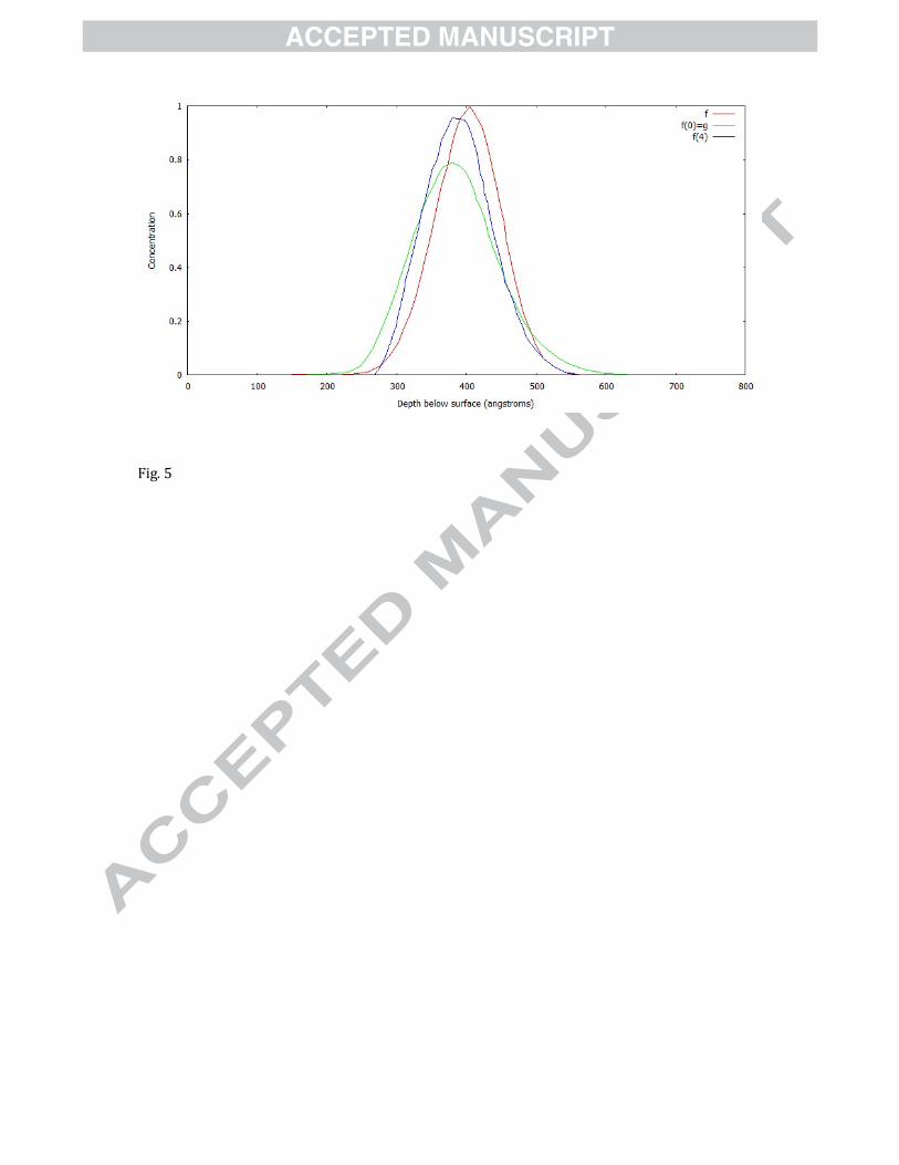
Fig. 5

Fig. 6

Fig. 7

Fig. 8