The Interplay Between Modulation

and Channel CodingMatthew C. Valenti∗ and Mohammad Fanaei†

∗Lane Department of Computer Science and Electrical Engineering,

West Virginia University, Morgantown, WV, USA.† Iron Range Engineering Program,

Minnesota State University at Mankato, Mankato, MN, USA.∗valenti@ieee.org, †mohammad.fanaei@ire.mnscu.edu

Abstract

Almost all modern communication systems employ some form of error-control coding. Oftentimes,

the coding is combined with high-order modulation, such as quadrature-amplitude modulation (QAM).

The question then becomes how best to combine coding and modulation. Such systems are typically

referred to as coded-modulation systems. This article investigates coded modulation systems with a

particular emphasis on the interface between the code and the modulation. As a pragmatic solution, bit-

interleaved coded modulation (BICM) is the main focus. With BICM, the output of a binary encoder is

passed through an interleaver, which permutes the ordering of the bits. The resulting permuted sequence

is then used to drive a standard M-ary modulator. A derivation of the receiver structure is provided, with

particular care being made in describing how the soft demapper (the device that reverses the modulation)

creates soft bit estimates that can then be used by a standard binary decoder. In addition to standard

BICM reception, the article also discusses BICM with iterative decoding (BICM-ID), which passes soft

outputs from the decoder back to the dempapper so that it can be used to iteratively refine the estimate

of the message.

Index Terms

Error-control coding, BICM, BICM-ID, High-order modulation, soft-decision decoding.

2

I. INTRODUCTION

The error rates achieved in standard uncoded digital modulation schemes are usually too

high to provide the quality of experience demanded by today’s applications. Almost all modern

communication systems use error-control coding to bring the error rate down to an acceptable

level. Error-control coding adds controlled redundancy to the transmission, and this redundancy

can be used to either correct or detect errors induced by the communication channel. While

correction of errors is preferred, even the detection of uncorrectable errors is useful insomuch

that can be used to automatically trigger a retransmission. Error detection is a critical ingredient

in any system that uses automatic repeat request (ARQ). Often, error correction and detection

are combined in hybrid-ARQ systems, which first attempt to correct errors, but request a

retransmission when uncorrectable errors are detected [1].

Particular care must be taken when a system uses both error-control coding and digital

modulation. Systems that combine the two are referred to as coded-modulation systems, though

often the term is reserved for systems that combine a code with a higher-order (non-binary)

modulation format such as QAM. In an uncoded system, modulation symbols are independently

selected one at a time, or from a limited memory of past symbols, as in continuous-phase

modulation (CPM). If the modulation constellation has M symbols, then each symbol is selected

using only m , log2(M) information bits. In contrast, a coded-modulation system groups

symbols together into modulated codewords that can be fairly long, with a typical codeword

containing hundreds or thousands of symbols, and a fairly long message is used to pick codewords

from a quite large codebook.

Let Ns denote the number of symbols in a modulated codeword and Nd denote the

dimensionality of each symbol. The encoded and modulated message can be represented by

a length-Ns vector x of symbols called a codeword.1 If vector modulation is used, then the ith

entry of x is in itself a length-Nd vector of real numbers, and it is convenient to arrange the

1Note that in this article, a codeword is a vector of modulated symbols rather than a vector of bits. In the case of binary

modulation, the two perspectives are equivalent.

3

codeword as an Nd-by-Ns matrix; i.e.,

x ,[x1 x2 . . . xNs

]=

x1,1 x1,2 . . . x1,Ns

x2,1 x2,2 . . . x2,Ns

...... . . . ...

xNd,1 xNd,2 . . . xNd,Ns

. (1)

Alternatively, xi, i = 1, 2, . . . , Ns, may be a real scalar if the modulation is one dimensional

(e.g., binary phase-shift keying (BPSK)) or a complex scalar if it is two dimensional (e.g.,

phase-shift keying (PSK) or QAM). Each symbol in x is drawn from the Nd-dimensional symbol

constellation X . Since each element of the codeword x must contain a symbol from X , it follows

that the codeword x must be drawn from the Cartesian product of Ns constellations X , and this

set is denoted by XNs . If the system were uncoded, then all MNs elements of XNs could be

used to convey mNs bits per codeword. However, this is an uninteresting usage case, as it is

the same thing as simply sending a sequence of Ns uncoded symbols, which will not provide

any coding gain.

In a coded-modulation system, each codeword must be drawn from a subset of XNs called

a codebook or simply a code. Here, we use Xc to denote the codebook, where Xc ⊂ XNs .

An encoder uses a vector of information bits u to select a codeword x ∈ Xc. Let Kb denote

the number of bits in u. As there is a one-to-one mapping between u and x, it follows that

Kb = log2 |Xc|, which is less than the number of bits that could be mapped when the system is

uncoded; i.e., log2MNs = mNs. The rate Rc = Kb/(mNs) of the code is the ratio of the number

of information bits actually conveyed by a codeword to the number of bits that could have been

sent had a code not been used (i.e., had the codeword been drawn from the full set XNs). Note that

Rc ≤ 1 since Xc ⊂ XNs , and hence Kb ≤ mNs. The rate quantifies the loss in spectral efficiency

due to the use of a code. A lower rate typically translates to a higher energy efficiency due to

the ability to correct more errors, though this comes at the cost of requiring more bandwidth for

a given data rate or a reduction in the data rate for a given bandwidth. The spectral efficiency

ηc of the coded modulation is the amount of information conveyed per transmitted symbol; i.e.,

ηc , mRc. Spectral efficiency is expressed in units of bits per channel use (bpcu). Often, the

loss in bandwidth efficiency due to using a lower-rate code can be compensated by simply using

a higher-order modulation. For instance, a system that uses 16-QAM modulation and half-rate

encoding (Rc = 1/2) might offer better energy efficiency than an uncoded quaternary phase-shift

4

keying (QPSK) system, even though the two systems have exactly the same bandwidth efficiency

(i.e., ηc = 2 bpcu).

The encoding operation is, therefore, characterized as a mapping of information bit sequences

of length Kb to modulation symbol sequences of length Ns. Conceptually, coded modulation

can be considered simply as a type of digital modulation with a very large signal set. Instead of

using m bits to select from among the M symbols in X , Kb bits are used to select modulated

codewords from Xc. Whereas the dimensionality of X is Nd, the set Xc has a dimensionality

of NdNs. The goal of the decoder is to determine the codeword in Xc that lies closest to the

received signal. In an additive white Gaussian noise (AWGN) channel, the measure of closeness

can be Euclidean distance, just as it is for uncoded modulation. The error performance for a

coded-modulation system in AWGN can be found from the standard Union bound, but with the

modulated codewords from Xc in used place of the symbols from X .

While considering a coded-modulation system as a vastly expanded constellation is simple

conceptually, there are several practical considerations that must be taken into account when

implementing coded modulation. One key issue is how to match the error-correction code with the

modulation. Some coded-modulation systems tightly integrate the two operations; for instance,

in a trellis-coded modulation (TCM) system [2], [3], a convolutional encoder is used, and the

branches of the encoder’s trellis are labelled with modulation symbols from X . TCM was widely

used for telephone-line modems in the late 1980’s and early 1990’s. However, as many powerful

codes are binary, the trend with modern systems is to combine a binary error-correction code

with a higher-order modulation. A pragmatic approach to coded modulation is to simply combine

an off-the-shelf binary code, such as a convolutional, turbo, or low-density parity-check (LDPC)

code, with a conventional non-binary modulation, such as QAM or PSK [4]. The output of the

binary encoder is fed into the input of the modulator. Often, for reasons that will be explained

later in the article, the bits output by the encoder are interleaved, i.e., their order is permuted,

before being fed into the modulator. Coded-modulation formats that are generated by placing an

interleaver between the output of a binary encoder and the input of a non-binary modulator are

called bit-interleaved coded modulation (BICM) [5], [6]. BICM is known to perform especially

well in fading environments [5], but is also often applied in AWGN environments due to its

convenience.

A key consideration in engineering coded-modulated systems is how to design the corre-

5

sponding receiver. If coded modulation is interpreted as an expansion of the signal set, then a

naıve brute-force decoder could operate by comparing the received signal against every candidate

codeword in Xc. While such a brute-force approach is reasonable for an uncoded system with

its M candidates, the number of candidates in a coded-modulation system grows exponentially

with the length of codeword. Clearly, such a decoder is not a viable choice except when the

codewords are extremely short. A more pragmatic approach is to perform demodulation and

decoding as two separate operations in the receiver. This is the approach taken in most coded-

modulation systems, especially BICM. For such receivers, the interface between the demodulator

and decoder is crucial. Here, we use the term channel decoder to describe the unit used to

decode just the binary channel code. On the one hand, the demodulator could provide hard

decisions of the individual coded bits to the channel decoder, and these hard decisions could

be processed by a hard-decision decoder. However, it is well known that soft-decision decoders

can significantly outperform hard-decision ones, and it is advantageous for the demodulator to

pass appropriately defined soft values to the channel decoder. A key aspect of this article is to

describe how to compute metrics suitable for soft-decision decoding. Moreover, performance in a

BICM system can often be improved by feeding back soft information from the channel decoder

to the demodulator and operating in an iterative mode called BICM with iterative decoding

(BICM-ID) [7].

This article is not meant to be a tutorial on error-control coding. There is by now a vast

literature on coding theory and practice; see, for instance, [8], [9], [10], [11], [12] and the

references therein. Rather than delving into the principles of code design, we consider a code

to merely be an arbitrary set of codewords without elaborating on how to design a good code.

Similarly, rather than describing the inner workings of the channel decoder, we consider it to

be a kind of black box that takes in appropriately defined soft-decision metrics and produces

estimates of the message. The main focus of the article is on the interfaces between modulation

and coding and in particular, the processing that must be done on the received signal to put

it into a format that can be used by an “off-the-shelf” channel decoder. To this end, the main

emphasis of the article is on the concepts of BICM and BICM-ID.

The remainder of this article is structured as follows. Section II presents a model of coded

modulation. Next, Section III derives the receiver for the case that the coded-modulation system

uses a binary modulation, such as BPSK. The receiver for the case that the modulation uses

6

non-binary constellations is considered in Section IV, and this includes receivers for both BICM

and BICM-ID architectures.

II. CODED MODULATION

A message vector is composed of Kb consecutive input information bits and denoted by u ,

[u1, u2, . . . , uKb], where each ui ∈ {0, 1}. As shown by the dashed box at the top of Figure 1,

the message vector is passed to a bit-to-symbol encoder that generates a length-Ns vector of

M -ary symbols denoted by x , [x1,x2, . . . ,xNs ]. Each component of x is a length-Nd column

vector of real numbers representing a single symbol drawn from the Nd-dimensional modulation

constellation X .

In general, the coded modulation can use any arbitrary one-to-one mapping from u to x.

However, for the remainder of this articlearticle, we will focus specifically on BICM, for which

the bit-to-symbol encoder comprises the three components shown inside the top dashed box of

Figure 1. In particular, the message vector u is passed to a binary channel encoder, which adds

controlled redundancy to it and produces a length-Kc binary codeword c , [c1, c2, . . . , cKc ],

where Kc ≥ Kb and each ci ∈ {0, 1}. The binary channel codebook is denoted by C, which is

the set of all valid binary codewords c, and the rate of the binary channel code is Rc = Kb/Kc

information bits per coded bit.

The binary codeword c can be directly fed to a bit-to-symbol mapper to generate the vector

of modulated symbols x. However, in a BICM system, each binary codeword is passed through

a pseudo-random, bit-wise interleaver Π that randomly permutes its input bits. The interleaver

essentially transforms the single channel with M -ary inputs into a set of m parallel binary

channels. Moreover, it is assumed that the interleaver arranges its output in the form of an

m-by-Ns matrix v as follows:

v ,[v1 v2 . . . vNs

]=

v1,1 v1,2 . . . v1,Ns

v2,1 v2,2 . . . v2,Ns

...... . . . ...

vm,1 vm,2 . . . vm,Ns

, (2)

where Ns , Kc/ log2M and v` is a (column) vector representing the `th column of the matrix.

Placing the interleaved bits into a matrix makes it clear that there is a one-to-one correspondence

7

Binary Encoder

Bit-wise Interleaver

Π

Bit-to-Symbol Mapper

µ

DecoderDeinterleaver

Π-1 Soft

Demapper

u c v

zlu

n

x

y

Symbol Encoder

Symbol Decoder

u

u

n

x

y

Binary

Encoder

BPSK

Mapper

µ

Binary

Decoder

Soft

Demapper

u c

z

n

x

yu

Bit-to-Symbol EncoderBICM Receiver

Bit-to-Symbol Encoder

Binary

Encoder

Bit-wise

Interleaver

Π

Bit-to-Symbol

Mapper

µ

Binary

Decoder

Deinterleaver

Π-1

Soft

Demapper

u c v

zl

n

x

y

Bit-wise

Interleaver

Π BICM-ID Receiver

u

λ

Fig. 1. Block diagram of a typical communication system with AWGN channel. The difference between BICM and BICM-ID

systems is that in a BICM system, there is no feedback information from the binary channel decoder to the demapper.

between columns of this matrix and the modulated symbols, and it also underscores the

perspective that the rows of the matrix correspond to the parallel binary channels created by

BICM.

The bit-to-symbol mapper function µ(·), defined as µ : {0, 1}m → X , converts each length-

m column of the matrix of interleaved coded bits v into an M -ary symbol drawn from a

constellation X , where x` , µ (v`), ` = 1, 2, . . . , Ns, is an Nd-dimensional column vector of real

numbers representing the M -ary modulated symbol associated with the `th column of matrix v.

Therefore, the final output of the mapper is an Nd-by-Ns matrix of modulated symbols x, as

defined in (1). The spectral efficiency of the system is ηc , Kb log2M/Kc = mRc bits per

channel use.

The vector of the modulated symbols x is assumed to be transmitted over an AWGN channel

and is received as

y = x + n, (3)

where y , [y1,y2, . . . ,yNs ] is the channel output and n , [n1,n2, . . . ,nNs ] is the uncorrelated,

8

identically distributed, zero-mean Gaussian channel noise, where the variance of each component

is σ2n , N0/2. The dimensionality of y` and n`, ` = 1, 2, . . . , Ns, equals to that of the modulation

scheme; i.e., y` and n` are Nd-dimensional column vectors.

Upon receiving the channel output y, the demapper calculates a metric for each interleaved

coded bit vi,`, i = 1, 2, . . . ,m and ` = 1, 2, . . . , Ns, which denotes the element in the ith row

and `th column of matrix v. In a BICM system, the metrics are de-interleaved and then fed to

the binary channel decoder. The channel decoder estimates the binary codeword from the set of

2Kb codewords based on the received metrics for coded bits from the demapper. Since there is

a one-to-one mapping between the vectors of information bits and binary codewords, deciding

on the most likely codeword is equivalent to the most likely vector of information bits, denoted

by u.

If the binary channel decoder is a soft-output decoder, it can produce a metric related to the

likelihood of each code bit. In a system with iterative decoding (ID), the soft output of the

channel decoder can be fed back to the demapper to improve its performance. In a BICM-ID

system, the soft information fed back from the channel decoder is interleaved before being fed

back to the demapper.

In the rest of this article, we analyze a generic BICM-ID system as shown in Figure 1. To

that end, we will first consider a coded-modulation system with binary signal constellation.

Following that, a BICM system is analyzed for the generic case of non-binary modulations.

Lastly, the receiver formulation is modified to consider the iterative decoding procedure.

III. RECEPTION OF CODED BINARY MODULATION

As a first step in analyzing the formulation of the receiver, consider a system with binary

channel coding and BPSK modulation over an AWGN channel. In this section, we study the

formulation of the demodulator and channel decoder for such a system. These formulations will

be generalized to an arbitrary, non-binary modulation scheme in the next sections. The coded-

modulation system under study is shown in Figure 2. Notice that the output of the binary encoder

is fed directly into a BPSK mapper. Since BPSK is binary, there is no need to use an interleaver

to partition the encoder output into parallel binary channels; thus, there is no interleaver in this

model.

BPSK is a one-dimensional modulation (i.e., Nd = 1) whose constellation contains M = 2

9

Binary Encoder

Bit-wise Interleaver

Π

Bit-to-Symbol Mapper

µ

DecoderDeinterleaver

Π-1 Soft

Demapper

u c v

zlu

n

x

y

Symbol Encoder

Symbol Decoder

u

u

n

x

y

Bit-to-Symbol EncoderBICM Receiver

Bit-to-Symbol Encoder

Binary

Encoder

Bit-wise

Interleaver

Π

Bit-to-Symbol

Mapper

µ

Binary

Decoder

Deinterleaver

Π-1

Soft

Demapper

u c v

zl

n

x

y

Bit-wise

Interleaver

Π BICM-ID Receiver

u

Binary

Encoder

BPSK

Mapper

µ

Binary

Decoder

Soft

Demapper

u c

z

n

x

yu

Fig. 2. Block diagram of a coded-modulation system with AWGN communication channel.

signal points with equal energy and opposite phase; i.e., X ={−√Es,√Es}

, where Es = |xi|2

is the energy per modulated symbol. Each symbol modulates only m = 1 bit; hence, Ns = Kc.

The elements of the vector of modulated symbols x are scalar and related to the corresponding

elements of binary codeword c by

xi =√Es(2ci − 1), i = 1, 2, . . . , Ns. (4)

The mapping given by (4) represents a code bit ci = 1 as a positive signal level xi = +√Es,

and a code bit ci = 0 as a negative signal level xi = −√Es.

A. Soft Demapping

Since BPSK modulation is memoryless, the demodulation of the received vector y can be

decomposed into the independent demodulation of its components. Upon reception of yi, i =

1, 2, . . . , Ns, the soft demapper calculates a metric for the coded bit associated with it. This

metric is defined to be in the form of a log-likelihood ratio (LLR), which is defined for the ith

coded bit as

zi , logP (ci = 1|yi)P (ci = 0|yi)

, i = 1, 2, . . . , Ns, (5)

where P (ci = b|yi), b = 0, 1, is the a priori conditional probability that ci = b, given that the

received symbol is yi, and the logarithm is usually assumed to be the natural logarithm (i.e.,

log ≡ ln). Note that the value of LLR is a function of the received symbol at the channel output.

10

Based on the relationship between coded bits and modulated symbols in (4), the above LLR can

be rewritten as

zi = logP(xi =

√Es|yi

)P(xi = −

√Es|yi

) . (6)

Using Bayes’ rule, P (xi|yi) can be written as

P (xi|yi) =fYi (yi|xi)P (xi)

fYi (yi), (7)

where fYi (yi|xi) denotes the conditional probability density function (pdf) of the received symbol

yi, given that the transmitted modulated symbol is xi. Substituting (7) into (6) and canceling

the common terms results in

zi = logfYi(yi|xi =

√Es)P(xi =

√Es)

fYi(yi|xi = −

√Es)P(xi = −

√Es) . (8)

Since the channel is assumed to be AWGN based on (3), yi conditioned on xi is a Gaussian

random variable with mean xi and variance N0/2; i.e., yi|xi ∼ N (xi, N0/2). Therefore,

fYi (yi|xi) =1√πN0

exp

(−(yi − xi)2

N0

). (9)

Substituting (9) in (8) and assuming equally likely coded bits, i.e., P(xi = −

√Es)

=

P(xi =

√Es), will result in the value of the LLR for BPSK modulation over an AWGN channel:

zi = ln

1√πN0

exp[− 1N0

(yi −√Es)2]

1√πN0

exp[− 1N0

(yi +√Es)2]

= − 1

N0

[(yi −

√Es)2−(yi +

√Es)2]

=4√Es

N0

yi.

(10)

The LLR values calculated by the demodulator will be used by the channel decoder to find the

most likely transmitted binary codeword c.

B. Channel Decoding

Now let’s consider how the channel decoder can use the bit LLRs from the demapper to

estimate the binary codeword from C. Given y, the maximum a posteriori probability (MAP)

decoding rule is

c = arg maxc∈C

P (c|y). (11)

11

Because the binary codeword c is mapped to the vector of modulated symbols x through the

one-to-one mapping x = µ(c), it can be replaced by the corresponding vector of modulated

symbols x in the above equation:

c = arg maxx∈Xc

P (x|y). (12)

where Xc is the set of modulated codewords; i.e., Xc , {x : c = µ−1(x) ∈ C}.

Since the components ni of the channel noise vector are independent, it follows that the set

of conditional probabilities P (xi|yi) are independent, and the above equation can be expressed

as

c = arg maxx∈Xc

Ns∏i=1

P (xi|yi). (13)

By dividing each term in the above multiplication by P (xi = −√Es|yi), the above equation can

be written as

c = arg maxx∈Xc

Ns∏i=1

P (xi|yi)P (xi = −

√Es|yi)

. (14)

Taking the logarithm, it can be rewritten as

c = arg maxx∈Xc

log

(Ns∏i=1

P (xi|yi)P (xi = −

√Es|yi)

)

= arg maxx∈Xc

Ns∑i=1

log

(P (xi|yi)

P (xi = −√Es|yi)

).

(15)

If the ith bit of the candidate codeword c is ci = 1, then xi =√Es, and the corresponding

term in (15) is

logP(xi =

√Es|yi

)P(xi = −

√Es|yi

) = zi. (16)

Notice that this is the LLR of xi given yi, as defined in (6). Similarly, if the ith bit of the

candidate codeword c is ci = 0, then xi = −√Es, and the corresponding term in (15) is

logP(xi = −

√Es|yi

)P(xi = −

√Es|yi

) = 0. (17)

Generalizing (16) and (17), the ith term of the sum in (15) is

log

(P (xi|yi)

P (xi = −√Es|yi)

)= cizi, (18)

12

and thus (15) may be written as

c = arg maxc∈C

Ns∑i=1

cizi. (19)

To summarize, decoding proceeds by first finding the LLR of each coded bit ci, which for

BPSK modulation over an AWGN channel is found using (10). For each one of the 2Kb candidate

codewords c ∈ C, the metric

Λ(c|y) ,Ns∑i=1

cizi (20)

is found. The most likely binary codeword is then the one with the largest metric given by (20).

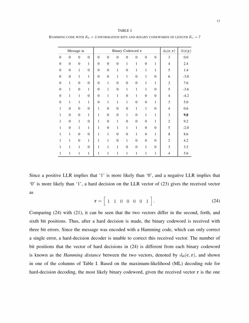
C. Example: Decoding of a Hamming Code

Let’s consider the decoding of a simple Hamming code with BPSK modulation over an AWGN

channel. Hamming codes are a class of single error-correction codes, characterized by having

codeword length Kc = 2q − 1 and message length Kb = 2q − 1− q for any integer q = Kc−Kb

[13]. A Hamming code with q = 3 is listed in Table I. For each codeword, a corresponding

message is shown. We note that the code is systematic since each message is disposed in the

first Kb bits of its corresponding binary codeword. The last two columns in the table will be

used in reference to the example decoding operation discussed below.

Suppose that the message vector of information bits is

u =[

1 0 0 1]

so that the corresponding binary codeword is

c =[

1 0 0 1 0 1 1]. (21)

Assume that the binary codeword is BPSK modulated based on (4) and sent over an AWGN

channel, where the variance of the additive channel noise is σ2n = N0/2 = 1 ≡ 0 dB. Let the

average energy per modulated symbol be Es = 1. Suppose that the received signal at the receiver

is

y =[

2.1 0.5 −0.9 −0.5 −1.7 −0.1 3.4]. (22)

Using (10), the vector of LLRs z , [z1, z2, . . . , zNs ] can be found for this example to be

z =4√Es

N0

y =[

4.2 1.0 −1.8 −1.0 −3.4 −0.2 6.8]. (23)

13

TABLE I

HAMMING CODE WITH Kb = 4 INFORMATION BITS AND BINARY CODEWORDS OF LENGTH Kc = 7

Message u Binary Codeword c dH(c, r) Λ(c|y)

0 0 0 0 0 0 0 0 0 0 0 3 0.0

0 0 0 1 0 0 0 1 1 0 1 4 2.4

0 0 1 0 0 0 1 0 1 1 1 5 1.4

0 0 1 1 0 0 1 1 0 1 0 6 -3.0

0 1 0 0 0 1 0 0 0 1 1 2 7.6

0 1 0 1 0 1 0 1 1 1 0 5 -3.6

0 1 1 0 0 1 1 0 1 0 0 4 -4.2

0 1 1 1 0 1 1 1 0 0 1 3 5.0

1 0 0 0 1 0 0 0 1 1 0 4 0.6

1 0 0 1 1 0 0 1 0 1 1 3 9.8

1 0 1 0 1 0 1 0 0 0 1 2 9.2

1 0 1 1 1 0 1 1 1 0 0 5 -2.0

1 1 0 0 1 1 0 0 1 0 1 1 8.6

1 1 0 1 1 1 0 1 0 0 0 2 4.2

1 1 1 0 1 1 1 0 0 1 0 3 3.2

1 1 1 1 1 1 1 1 1 1 1 4 5.6

Since a positive LLR implies that ‘1’ is more likely than ‘0’, and a negative LLR implies that

‘0’ is more likely than ‘1’, a hard decision on the LLR vector of (23) gives the received vector

as

r =[

1 1 0 0 0 0 1]. (24)

Comparing (24) with (21), it can be seen that the two vectors differ in the second, forth, and

sixth bit positions. Thus, after a hard decision is made, the binary codeword is received with

three bit errors. Since the message was encoded with a Hamming code, which can only correct

a single error, a hard-decision decoder is unable to correct this received vector. The number of

bit positions that the vector of hard decisions in (24) is different from each binary codeword

is known as the Hamming distance between the two vectors, denoted by dH(c, r), and shown

in one of the columns of Table I. Based on the maximum-likelihood (ML) decoding rule for

hard-decision decoding, the most likely binary codeword, given the received vector r is the one

14

with the least number of bit differences with r, which is

cHD =[

1 1 0 0 1 0 1], (25)

which is not the transmitted binary codeword.

Now consider the soft-decision decoder. For each binary codeword in C, the metric Λ(c|y)

is computed using (20), and the binary codeword with the highest metric is selected. For the

Hamming code shown in Table I and the LLR vector given by (23), the corresponding metric for

each one of the 2Kb = 16 binary codewords is given in the last column of Table I. The maximum

metric is Λ(c|y) = 9.8, which corresponds to the binary codeword cSD = [1 0 0 1 0 1 1]. This

is the transmitted binary codeword, as specified by (21). Thus, the soft-decision decoder has

successfully decoded the received vector, despite the fact that it contained three errors when

subjected to a hard decision.

IV. RECEPTION OF CODED NONBINARY MODULATION

In this section, we extend the formulation of the receiver in Section III to memoryless, non-

binary modulations to include bit-wise interleaver Π between the channel encoder and bit-to-

symbol mapper as well as iterative decoding at the receiver.

A. BICM Reception

Since the modulation scheme is assumed to be memoryless, the demodulation of the

received vector y can be decomposed into the independent demodulation of its symbols y`,

` = 1, 2, . . . , Ns. Upon reception of y`, the soft demapper calculates a metric for each one of

the m bits associated with the `th column of the transmitted matrix v. This metric is defined to

be in the form of an LLR, which is defined for the ith bit in the `th column of matrix v as

zi,` , logP (vi,` = 1|y`)P (vi,` = 0|y`)

, i = 1, 2, . . . ,m and ` = 1, 2, . . . , Ns. (26)

Note that the LLR value for each one of the m bits associated with the `th column of the

transmitted matrix of bits only depends on the `th column of the received matrix y. The above

LLR can be rewritten as

zi,` = log

∑s∈X 1

iP (s|y`)∑

s∈X 0iP (s|y`)

, i = 1, 2, . . . ,m and ` = 1, 2, . . . , Ns, (27)

15

where X bi is the set of the modulated symbols for which the ith bit in the mapped column v` to

the symbol s ∈ X is equal to b, where b = 0, 1. In other words,

X bi ,

{s∣∣v , µ−1 (s) and vi = b

}, b = 0, 1 and i = 1, 2, . . . ,m.

Using Bayes’ rule, P (s|y`) can be written as

P (s|y`) =fY`

(y`|s)P (s)

fY`(y`)

, (28)

where fY`(y`|s) denotes the conditional pdf of the received signal y`, given that the transmitted

modulated symbol is x` = s. Substituting (28) into (27) and canceling the common terms results

in

zi,` = log

∑s∈X 1

ifY`

(y`|s)P (s)∑s∈X 0

ifY`

(y`|s)P (s). (29)

Since the channel is assumed to be AWGN based on (3), Y`|s is a Gaussian random vector

with mean s and covariance matrix N0

2INd

, where INdis the Nd-by-Nd identity matrix; i.e.,

Y`|s ∼ N(s, N0

2INd

). Therefore,

fY`(y`|s) =

1

(πN0)Nd/2

exp

(−(y` − s) (y` − s)T

N0

)(a)∝ exp

(− 1

N0

‖y` − s‖2),

(30)

where ‘∝’ is read as “is proportional to”, ‖·‖ denotes the L2-norm of a vector, ‖y`− s‖ denotes

the Euclidean distance between vectors y` and s, and (a) is because the common terms in the

numerator and denominator of (29) can be canceled out. Substituting (30) in (29) results in

zi,` = log

∑s∈X 1

iexp

(− 1N0‖y` − s‖2

)P (s)∑

s∈X 0i

exp(− 1N0‖y` − s‖2

)P (s)

. (31)

Note that the bit LLR found in (31) is a function of the Euclidean distance between the received

signal y` and each one of the M = 2m modulated symbols in the constellation s ∈ X .

In a BICM system, all of the modulated symbols are assumed to be equally likely so that the

term P (s) cancels in the numerator and denominator of (31), and the MAP bit metric defined

in (26) is reduced to the ML bit metric. Therefore, the bit LLR defined in (26) can be found in

a BICM system as

zi,` = log

∑s∈X 1

iexp

(− 1N0‖y` − s‖2

)∑

s∈X 0i

exp(− 1N0‖y` − s‖2

) . (32)

16

The bit LLR can be computed using the Jacobian logarithm [14], [15], [16]

ln(eα + eβ

)= max (α, β) + ln

(1 + e−|α−β|

)= max (α, β) + γc (|α− β|) ,

(33)

where γc (·) is a one-dimensional correction function, which is a function of only the difference

between the two variables α and β. Based on this identity, the following operator is defined [16]:

max∗ (α, β) , ln(eα + eβ

). (34)

Similar to the property of the ‘max’ operator for which

max (α1, α2, α3) = max (max (α1, α2) , α3) ,

the ‘max∗’ operator can be extended to more than two variables as

max∗ (α1, α2, α3) = max∗(

max∗ (α1, α2) , α3

).

Therefore, the ‘max∗’ operator can in general be defined as

max∗α∈{α1,α2,...,αt}

g(α) , max∗ (g (α1) , g (α2) , . . . , g (αt)) = lnt∑

q=1

exp (g (αq)) , (35)

where g(·) is an arbitrary function.

Based on the definition of the ‘max∗’ operator, Equation (32) can be rewritten as

zi,` = max∗s∈X 1

i

(− 1

N0

‖y` − s‖2)−max∗

s∈X 0i

(− 1

N0

‖y` − s‖2). (36)

Thus, the BICM receiver computes the LLR of each interleaved code bit by using (36), de-

interleaves the resulting LLRs to put them into a row vector that has the same ordering as c,

and then passes the result to the binary channel decoder.

B. BICM-ID Reception

In contrast with BICM systems, which assume all of the modulated symbols to be equally

likely during the demapping operation (i.e., P (s) = 1/M for s ∈ X ), BICM-ID systems attempt

to estimate the a priori likelihood of the modulated symbols iteratively using information fed

back from the soft-output binary decoder to the soft demapper. The soft information fed back

17

from the binary decoder is called the extrinsic information. Prior to being fed into the soft

demapper, it is interleaved and placed into a matrix λ of the form

λ ,[λ1 λ2 . . . λNs

]=

λ1,1 λ1,2 . . . λ1,Ns

λ2,1 λ2,2 . . . λ2,Ns

...... . . . ...

λm,1 λm,2 . . . λm,Ns

. (37)

Rather than assuming equally likely symbols with equal P (s), the BICM-ID receiver uses λ

to produce an a priori estimate that is used in place of P (s) in (31). During the `th symbol

interval, the estimate of P (s) is denoted by P (s|λ`) to emphasize that the estimate of the symbol

probability is found by using the `th column of matrix λ, denoted by λ`. It follows that for the

BICM-ID receiver, (31) becomes

zi,` = log

∑s∈X 1

iexp

(− 1N0‖y` − s‖2

)P (s|λ`)∑

s∈X 0i

exp(− 1N0‖y` − s‖2

)P (s|λ`)

. (38)

Let w denote the length-m vector of bits associated with s; i.e., s = µ(w) and w = µ−1(s).

Since there is a one-to-one mapping between s and w, it follows that P (s|λ`) = P (w|λ`).

Note that if s ∈ X bi , then the ith bit in the corresponding w is fixed to wi = b, where b ∈ {0, 1}.

Therefore, for any s ∈ X bi

P (s|λ`) = P (w|λ`)∣∣∣wi=b

= P (w\wi|λ`) , (39)

where w\wi is the vector w excluding element wi and P (w\wi|λ`) represents the estimate of

the a priori probability of w excluding its ith bit wi, which is found by using λ`.

Since it is a LLR, λi,` , ln P [wi=1]P [wi=0]

for the `th symbol. It follows that

P [wi = 0] =1

1 + eλi,`(40a)

P [wi = 1] =eλi,`

1 + eλi,`. (40b)

Generalizing (40a) and (40b), the a priori probability of each transmitted bit can be written as

P [wi] =

(eλi,`

)wi

1 + eλi,`. (41)

18

If wi = 0, (41) reduces to (40a), whereas if wi = 1, (41) reduces to (40b). The a priori probability

P (w\wi|λ`) can be written as

P (w\wi|λ`) =m∏j=1j 6=i

P [wj](a)= exp

m∑j=1j 6=i

lnP [wj]

(b)= exp

m∑j=1j 6=i

[wj ln eλj,` − ln

(1 + eλj,`

)]

= exp

m∑j=1j 6=i

wj λj,`

× exp

− m∑j=1j 6=i

ln(1 + eλj,`

) ,

(42)

where (a) is based on the identity a = exp (ln a), and (b) replaces P [wj] with (41) and uses the

identities log(a/b) = log(a)− log(b) and log(ab) = b log(a). During each iteration, Equation (42)

can be used to estimate the a priori probability of the modulated symbol P (s|λ`) by using λ`.

The substitution of this a priori information into (38) and cancellation of the common terms

between the numerator and denominator result in

zi,` = log

∑s∈X 1

iexp

(− 1N0‖y` − s‖2 +

∑mj=1j 6=i

wjλj,`

)∑

s∈X 0i

exp

(− 1N0‖y` − s‖2 +

∑mj=1j 6=i

wjλj,`

) . (43)

Based on the definition of the ‘max∗’ operator, Equation (43) can be rewritten as

zi,` = max∗s∈X 1

i

− 1

N0

‖y` − s‖2 +m∑j=1j 6=i

wjλj,`

−max∗s∈X 0

i

− 1

N0

‖y` − s‖2 +m∑j=1j 6=i

wjλj,`

. (44)

where the reader is reminded that w , µ−1 (s). As explained before, the above bit LLR’s are

de-interleaved and fed to the soft-input channel decoder so that it can estimate the vector of the

transmitted information bits u. The operation of the channel decoder is beyond the scope of this

article and depends on the structure of the binary channel code.

19

u

c(0)

c(1)

DD D D D D

Fig. 3. A rate-1/2 convolutional encoder with a constraint length of seven.

C. Example: BICM vs. BICM-ID

As an example, we compare the performance of BICM with BICM-ID. Throughout this

example, we use the same binary code, which is a rate Rc = 1/2 convolutional code. The

code is generated using the structure shown in Figure 3. Data is fed sequentially through the

encoder, which contains a linear shift register. During each bit period, the next message bit is

fed into the shift register, and two output bits are determined from the depicted logic. The output

bits form the binary codeword. The encoder shown in Figure 3 is said to have a constraint length

of seven, because each output bit can depend on up to seven bits (the current bit plus the six bits

stored in the shift register). The convolutional code is decoded with the max-log-MAP algorithm

[17]. For more information about convolutional codes, the reader is referred to [8], [18].

The performance of BICM and BICM-ID depends on the function µ(·) used to map bits to

symbols. In this example, we consider 16-QAM modulation with the two mappings shown in

Figure 4: a Gray mapping and an anti-Gray mapping. In the Gray mapping, the bits labeling

neighboring bit positions differ in just one bit position, whereas in the anti-Gray mapping, the

bits labeling neighboring bit positions are common in just one bit position. For reasons discussed

in [19], the Gray labeling is optimal when BICM is used, while the anti-Gray labeling is optimal

when BICM-ID is used.

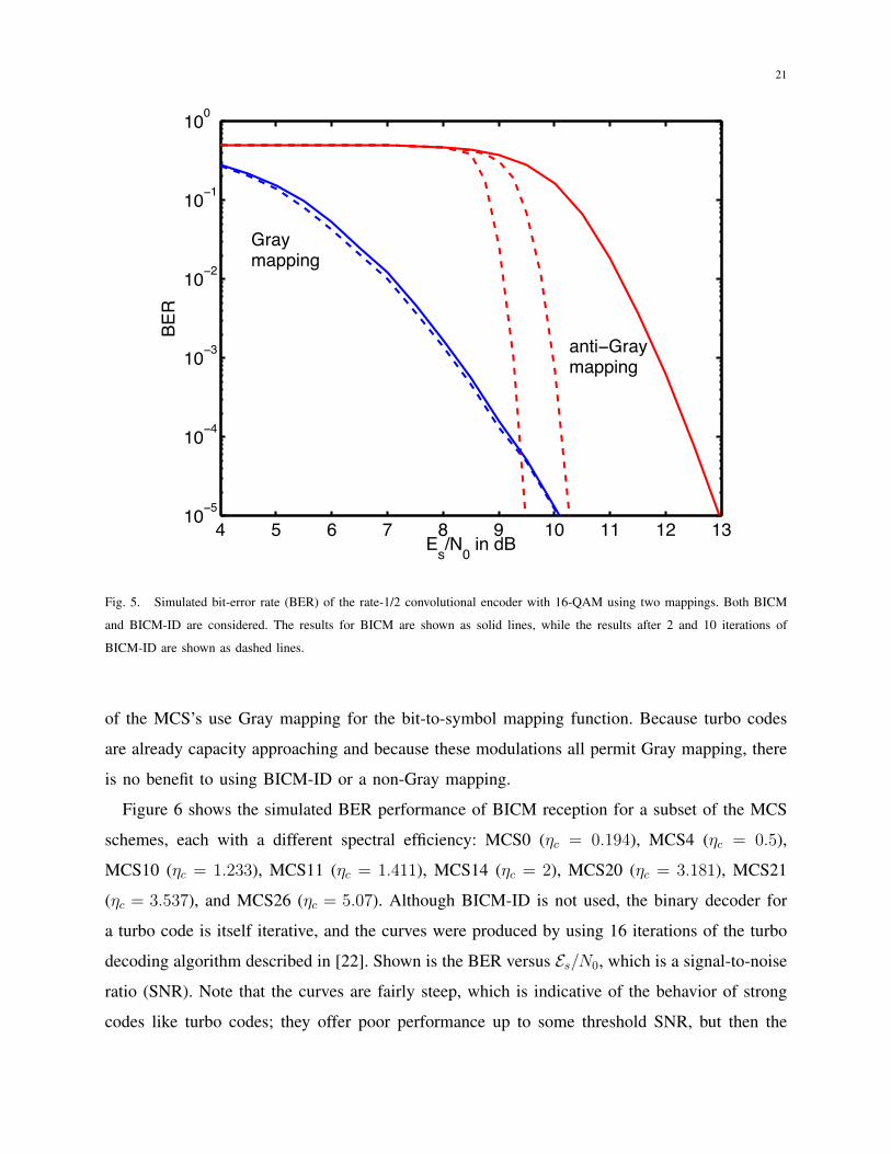
The results of a set of simulations using the binary code of Figure 3 and mappings of Figure 4

are shown in Figure 5. For each of the two mappings, both BICM and BICM-ID receivers are

considered. The results of BICM are shown as solid lines, while the results of BICM-ID are

shown as dashed lines. The curves show the bit error rate (BER) as a function of the ratio

of Es/N0, where N0 is the one-sided noise spectral density. An additive white Gaussian noise

20

1111 1011

1110 1010

0011 0111

0010 0110

1100 1000

1101 1001

0000 0100

0001 0101

0000 1101

0111 1010

0110 1011

0001 1100

1001 0100

1110 0011

1111 0010

1000 0101

Fig. 4. A Gray mapping (left subfigure) and an anti-Gray mapping (right subfigure).

(AWGN) channel is assumed.

If only BICM is used, then Gray mapping gives much better performance than anti-Gray

mapping. However, the opposite is true for BICM-ID. As shown in Fig. 5, the system with Gray

mapping shows only a negligible gain from BICM-ID — the figure shows results after 2 and

10 iterations, but there is no gain after the second iteration and hence, the two curves coincide.

However, the anti-Gray mapping shows a dramatic gain when BICM-ID is used. For bit-error

rates below 10−4, anti-Gray mapping with 10 iterations of decoding outperforms Gray mapping

(either with or without BICM-ID).

D. Example: LTE Turbo Codes

As another example of the bit-error performance of a coded-modulation system, we consider

the coded modulation used in the Long Term Evolution (LTE) 4G cellular system [20]. LTE

uses a combination of a turbo code [21], [22] and higher-order modulation, which may be

QPSK, 16-QAM, or 64-QAM. LTE is an adaptive system, where the modulation and coding

scheme (MCS) switches on timescales on the order of a millisecond. LTE supports 27 MCS

schemes, with each MCS scheme being embodied by a particular combination of code rate and

modulation type. The MCS index is proportional to the spectral efficiency ηc. The eleven lowest

MCS’s (called MCS0 through MCS10) use QPSK, the 10 intermediate MCS’s (MCS11 through

MCS20) use 16-QAM, and the 6 highest MCS’s (MCS21 through MCS26) use 64-QAM. All

21

4 5 6 7 8 9 10 11 12 1310−5

10−4

10−3

10−2

10−1

100

Es/N0 in dB

BER

Graymapping

anti−Graymapping

Fig. 5. Simulated bit-error rate (BER) of the rate-1/2 convolutional encoder with 16-QAM using two mappings. Both BICM

and BICM-ID are considered. The results for BICM are shown as solid lines, while the results after 2 and 10 iterations of

BICM-ID are shown as dashed lines.

of the MCS’s use Gray mapping for the bit-to-symbol mapping function. Because turbo codes

are already capacity approaching and because these modulations all permit Gray mapping, there

is no benefit to using BICM-ID or a non-Gray mapping.

Figure 6 shows the simulated BER performance of BICM reception for a subset of the MCS

schemes, each with a different spectral efficiency: MCS0 (ηc = 0.194), MCS4 (ηc = 0.5),

MCS10 (ηc = 1.233), MCS11 (ηc = 1.411), MCS14 (ηc = 2), MCS20 (ηc = 3.181), MCS21

(ηc = 3.537), and MCS26 (ηc = 5.07). Although BICM-ID is not used, the binary decoder for

a turbo code is itself iterative, and the curves were produced by using 16 iterations of the turbo

decoding algorithm described in [22]. Shown is the BER versus Es/N0, which is a signal-to-noise

ratio (SNR). Note that the curves are fairly steep, which is indicative of the behavior of strong

codes like turbo codes; they offer poor performance up to some threshold SNR, but then the

22

−10 −5 0 5 10 15 2010−6

10−5

10−4

10−3

10−2

10−1

100

Es/N0 in dB

BER

QPSK

16QAM

64QAM

MCS0

MCS4

MCS10

MCS11

MCS14

MCS20

MCS21

MCS26

Fig. 6. Simulated bit-error rate (BER) of the code-modulation used by LTE.

performance rapidly improves with increasing SNR. As can be seen, codes of lower spectral

efficiency can operate at lower SNR values.

REFERENCES

[1] G. Caire and D. Tuninetti, “The throughput of hybrid-ARQ protocols for the Gaussian collision channel,” IEEE Trans.

Inform. Theory, vol. 47, no. 5, pp. 1971–1988, July 2001.

[2] G. Ungerboeck, “Trellis-coded modulation with redundant signal sets – Part I: Introduction,” IEEE Communications

Magazine, vol. 25, no. 2, pp. 5–11, February 1987.

[3] ——, “Trellis-coded modulation with redundant signal sets – Part II: State of the art,” IEEE Communications Magazine,

vol. 25, no. 2, pp. 12–21, February 1987.

[4] A. Viterbi, J. Wolf, E. Zehavi, and R. Padovani, “A pragmatic approach to trellis-coded modulation,” IEEE Communications

Magazine, vol. 27, no. 7, pp. 11–19, July 1989.

[5] G. Caire, G. Taricco, and E. Biglieri, “Bit-interleaved coded modulation,” IEEE Transactions on Information Theory,

vol. 44, no. 3, pp. 927–946, May 1998.

23

[6] L. Szczecinski and A. Alvarado, Bit-interleaved coded modulation: Fundamentals, analysis and design. John Wiley &

Sons, 2015.

[7] X. Li and J. Ritcey, “Trellis-coded modulation with bit interleaving and iterative decoding,” IEEE Journal on Selected

Areas in Communications, vol. 17, no. 4, pp. 715–724, April 1999.

[8] S. Lin and D. Costello, Error control coding: Fundamentals and applications, 2nd ed. New Jersey: Prentice Hall, 2004.

[9] T. K. Moon, Error correction coding: Mathematical methods and algorithms. John Wiley & Sons, 2005.

[10] D. Declercq, M. Fossorier, and E. Biglieri, Channel coding: Theory, algorithms, and applications, 1st ed. Academic

Press, 2014.

[11] W. E. Ryan and S. Lin, Channel codes: Classical and modern. Cambridge University Press, 2009.

[12] S. B. Wicker, Error control systems for digital communication and storage. Upper Saddle River, NJ, USA: Prentice-Hall,

Inc., 1995.

[13] R. W. Hamming, “Error detecting and error correcting codes,” Bell System Technical Journal, vol. 29, pp. 147–160, April

1950.

[14] J. Erfanian, S. Pasupathy, and P. Gulak, “Reduced complexity symbol detectors with parallel structure for ISI channels,”

IEEE Transactions on Communications, vol. 42, no. 2/3/4, pp. 1661–1671, February/March/April 1994.

[15] S. Pietrobon, “Implementation and performance of a serial MAP decoder for use in an iterative turbo decoder,” in IEEE

International Symposium on Information Theory (ISIT’95), Whistler, BC, Canada, September 1995, p. 471.

[16] A. Viterbi, “An intuitive justification and a simplified implementation of the MAP decoder for convolutional codes,” IEEE

Journal on Selected Areas in Communications, vol. 16, no. 2, pp. 260–264, February 1998.

[17] P. Robertson, P. Hoeher, and E. Villebrun, “Optimal and sub-optimal maximum a posteriori algorithms suitable for turbo

decoding,” European Transactions on Telecommunications, vol. 8, no. 2, pp. 119–125, March/April 1997.

[18] J. G. Proakis and M. Salehi, Digital Communications, 5th ed. New York, NY: McGraw-Hill, Inc., 2008.

[19] D. Torrieri and M. C. Valenti, “Constellation labeling maps for low error floors,” IEEE Transactions on Wireless

Communications, vol. 7, no. 12, pp. 5401–5407, 2008.

[20] E. Dahlman, S. Parkvall, and J. Skold, 4G LTE/LTE–Advanced for Mobile Broadband. Academic Press, 2011.

[21] C. Berrou and A. Glavieux, “Near optimum error correcting coding and decoding: Turbo codes,” IEEE Transactions on

Communications, vol. 44, no. 10, pp. 1261–1271, October 1996.

[22] M. C. Valenti and J. Sun, “The UMTS turbo code and an efficient decoder implementation suitable for software defined

radios,” International Journal of Wireless Information Networks, vol. 8, no. 4, pp. 203–216, October 2001.