Saïd Business School

Research Papers

Saïd Business School RP 2014-11

The Saïd Business School’s working paper series aims to provide early access to high-quality and rigorous academic research. The Shool’s working papers reflect a commitment to excellence, and an interdisciplinary scope that is appropriate to a business school embedded in one of the world’s major research universities. This paper is authorised or co-authored by Saïd Business School faculty. It is circulated for comment and discussion only. Contents should be considered preliminary, and are not to be quoted or reproduced without the author’s permission.

The International CAPM Redux

Francesca Brusa Saïd Business School, University of Oxford; Oxford-Man Institute of Quantitative Finance, University of Oxford

Tarun Ramadorai Saïd Business School, University of Oxford; Oxford-Man Institute of Quantitative Finance, University of Oxford; Centre for Economic Policy Research (CEPR)

Adrien Verdelhan Sloan School of Management, Massachusets Institute of Technology (MIT); National Bureau of Economic Research (NBER)

July 2014

The International CAPM Redux

Francesca Brusa Tarun Ramadorai Adrien Verdelhan∗

Abstract

We provide evidence that international investors are compensated for bearing

currency risk using a new three-factor international capital asset pricing model,

comprising a global equity factor denominated in local currencies, and two cur-

rency factors, dollar and carry. The model explains a wide cross-section of equity

returns from 46 developed and emerging countries from 1976 to the present, is also

useful at explaining the risks of international mutual funds and hedge funds, and

outperforms standard international asset pricing models. We explain our findings

using a simple complete-markets model with endogenous exchange rate risk, and

additionally derive new results on optimal currency investment in international

portfolios.

∗Brusa: Saıd Business School and Oxford-Man Institute of Quantitative Finance, University of

Oxford, Park End Street, Oxford OX1 1HP, UK. Email: fra.brusa@sbs.ox.ac.uk. Ramadorai: Saıd

Business School, Oxford-Man Institute of Quantitative Finance, University of Oxford, Park End Street,

Oxford OX1 1HP, UK, and CEPR. Email: tarun.ramadorai@sbs.ox.ac.uk. Verdelhan: MIT Sloan and

NBER. 100 Main Street, Cambridge, MA 02142, USA. Email: adrienv@mit.edu.

1 Introduction

Are international equity investors compensated for bearing exchange rate risk? This

question is increasingly relevant in light of the rapid acceleration of international fi-

nancial integration over the past three decades. Figure 1 shows that aggregate foreign

equity holdings as a percentage of global gross domestic product have increased steadily

from roughly 3% in the 1980s to approximately 30% in 2011, alongside a steady dis-

mantling of de-jure cross-border capital flow restrictions. The magnitudes are large,

highlighting the importance of this issue – in the United States, for example, foreign

equity holdings are currently worth roughly US$ 6 trillion.

In theory, exchange rate risk should matter to the pricing of equities and other risky

assets in a world of real rigidities and deviations from purchasing power parity. These

deviations affect the consumption of international investors, who invest abroad, but

consume at home. In most plausible theoretical international asset pricing models, this

effect on consumption leads to equilibrium compensation for the risk of low returns on

foreign investments once these returns are expressed in real domestic terms. Reasonable

though this rationale is, empirical work in international asset pricing, with a few notable

exceptions, has not been able to provide convincing evidence that currency risk is priced

in international equity markets.

In this paper, we present a new three-factor model to capture the risks in interna-

tional equity portfolios. These three factors are the return on a world market portfolio

denominated in local currency terms, and two currency factors which effectively sum-

marize variation in a broad cross-section of bilateral exchange rates, namely, the dollar

1

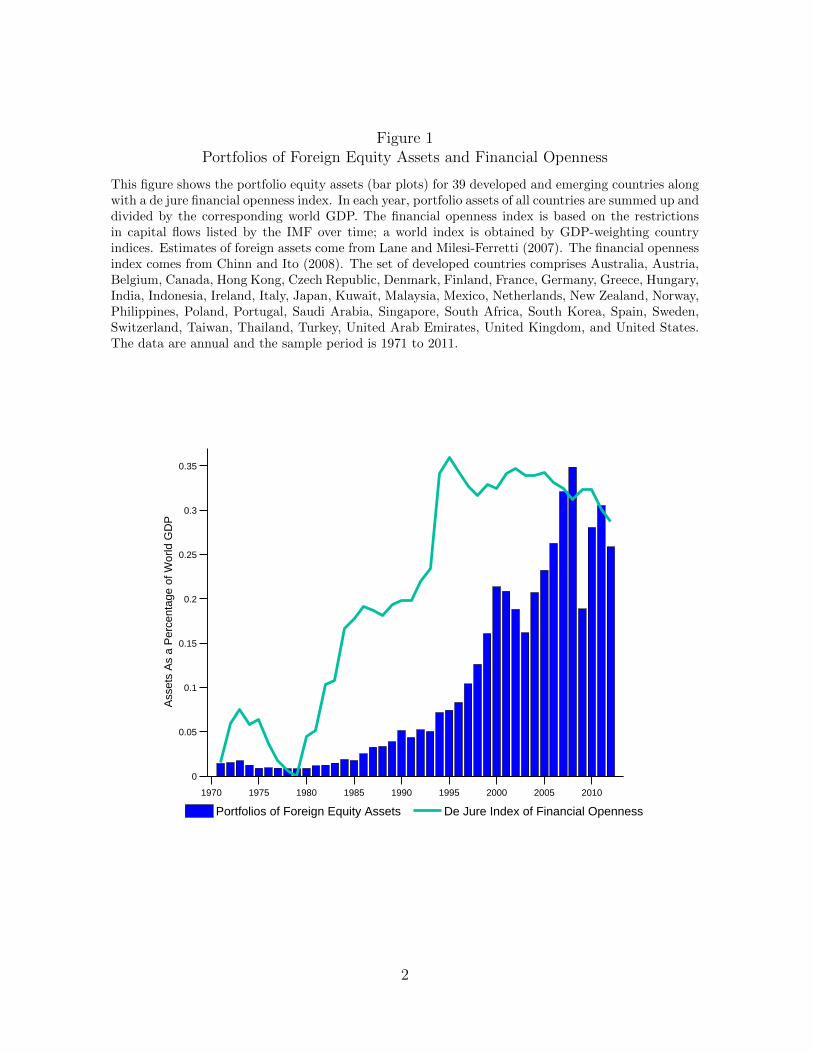
Figure 1Portfolios of Foreign Equity Assets and Financial Openness

This figure shows the portfolio equity assets (bar plots) for 39 developed and emerging countries alongwith a de jure financial openness index. In each year, portfolio assets of all countries are summed up anddivided by the corresponding world GDP. The financial openness index is based on the restrictionsin capital flows listed by the IMF over time; a world index is obtained by GDP-weighting countryindices. Estimates of foreign assets come from Lane and Milesi-Ferretti (2007). The financial opennessindex comes from Chinn and Ito (2008). The set of developed countries comprises Australia, Austria,Belgium, Canada, Hong Kong, Czech Republic, Denmark, Finland, France, Germany, Greece, Hungary,India, Indonesia, Ireland, Italy, Japan, Kuwait, Malaysia, Mexico, Netherlands, New Zealand, Norway,Philippines, Poland, Portugal, Saudi Arabia, Singapore, South Africa, South Korea, Spain, Sweden,Switzerland, Taiwan, Thailand, Turkey, United Arab Emirates, United Kingdom, and United States.The data are annual and the sample period is 1971 to 2011.

1970 1975 1980 1985 1990 1995 2000 2005 2010

0

0.05

0.1

0.15

0.2

0.25

0.3

0.35

Ass

ets

As

a P

erce

ntag

e of

Wor

ld G

DP

Portfolios of Foreign Equity Assets De Jure Index of Financial Openness

2

factor and the carry factor.1

To test the model, we compile a comprehensive dataset of equity returns spanning

value, size, and country aggregate portfolio returns from 25 developed markets and 21

emerging markets between February 1976 and April 2013. When estimated on these

data, the model delivers an important role for currency risk in the cross-section of equity

returns.

Importantly, in conditional asset pricing tests, our model outperforms the single-

global factor World CAPM as well as the International CAPM estimated by Dumas

and Solnik (1995), and delivers comparable performance to the global versions of the

popular Fama and French (2012) factors. We show that our model is also relevant

to those interested in delegated portfolios of international assets. It is often difficult

to infer the amount of currency risk taken on by international investment managers,

and our factors offer a simple metric of the extent of this issue, helping to explain a

significant fraction of the variation in international mutual and hedge fund returns.

To better understand the dynamics captured by the empirical risk factors, we build

a simple theoretical model in which exchange rates, currency risk factors, and equity

market returns are all precisely defined. In leading international equity asset pricing

models, exchange rate variation arises exogenously. In contrast exchange rates are

endogenous in our model, and to better explore the impacts of this important difference,

we simplify all other aspects of the model, assuming that financial markets are complete,

and writing down the law of motion of the lognormal stochastic discount factors (SDFs)

in all countries.

1Verdelhan (2014) shows that a substantial fraction of the variation in bilateral exchange rates canbe captured by these two factors. The dollar factor is the average excess return earned by an investorthat borrows in the U.S. and invests in a broad portfolio of foreign currencies. The carry factor is theaverage excess return earned by an investor that goes short (long) in a portfolio of low (high) interestrate currencies.

3

In our setup, country SDFs depend on country-specific shocks, as well as three global

shocks, and each country’s aggregate dividend growth rate also depends on the same set

of shocks. To create a role for a pure equity risk factor (which affects all countries in the

same way), we allow one of the global shocks to affect all SDFs similarly. Since changes

in exchange rates are differences in log SDFs, this global shock does not show up in

currency markets, resulting in a degree of segmentation between equity and currency

markets. This simple innovation to the basic complete markets model, namely, the

addition of the “equity” global shock, allows us to work in a very tractable framework

in which (realized and expected) equity and currency returns can be written down in

closed form.

The model reveals that the world aggregate equity return expressed in a common

currency actually does contain all relevant information necessary for pricing interna-

tional assets, meaning that there should be no role for bilateral exchange rates. The

twist is that time-variation in the prices of global shocks – necessary to account for

time-varying currency risk premia – confounds empirical estimation using a single-factor

model, especially when the relevant state variables are unknown to the econometrician.

We show that including the currency risk factors in our three-factor empirical model

arises as a natural solution to the challenges of empirical estimation in this framework.

We use the model to shed light on our main empirical results, calibrating it to match

a large set of equity and currency moments, and generating simulated data. We apply

exactly the same estimation procedure as we do on real data to these simulated data,

and replicate our empirical finding that the new “International CAPM Redux” outper-

forms both the World CAPM of Sharpe (1964) and Lintner (1965), and the “Classic”

International CAPM of Adler and Dumas (1983). We note that time-variation in the

prices of risk appears key to this result.

Finally, we use the model to revisit a longstanding and important issue in inter-

4

national finance, namely, optimal currency hedging in international portfolios.2 The

prevailing wisdom arises from the mean-variance efficient framework of Black (1989),

in which the optimal amount of currency hedging depends on the mean and standard

deviation of world market returns, as well as on exchange rate volatility. In other words,

Black (1989) shows that the optimal amount of currency hedging is constant through

time and across investor location. In contrast, in our model, in which exchange rates

are endogenous and driven by many of the same risks affecting equities, the optimal

amount of investment in currency portfolios such as carry and dollar is time-varying

and investor-location-specific, and depends on the prices of risk of both country-specific

and global shocks.

Our paper relates to two very large strands of literature on international equity

markets and on currency risk. A short paragraph in the introduction of this paper

would not do justice to this literature. Instead, we propose a four-page review of the

most relevant work. In the interest of space, the material is placed at the start of the

Appendix.

The paper is organized as follows. Section 2 shows the empirical specifications of the

various international asset pricing models that we test. Section 3 describes the data on

which we conduct these asset pricing tests, and Section 4 discusses the results. Section

5 presents our simple theoretical model which endogenizes exchange rates in complete

markets and gives rise to the empirical specification of the International CAPM Redux.

Section 6 shows how we can use the model to shed light on optimal hedging in a world

with endogenous exchange rates, and Section 7 concludes. All robustness checks and

2This continues to be a hot topic for both institutional and retail investors. For example, fourExchange-Traded Funds (ETFs) that seek to completely hedge the currency risk component of inter-national equity returns are among the ten fastest growing ETFs over the last six months, collectingmore than 30 billion dollars over this short period.

5

additional results that are mentioned but not reported in the paper are provided in the

Online Appendix.

2 Specifying and Testing International Asset Pric-

ing Models

We compare the performance of our three-factor model against a range of alternative

asset pricing models: the World CAPM, the International CAPM, and a global version

of the Fama-French-Carhart model. In this section, we briefly present the empirical

specifications of these leading international asset pricing models and contrast them with

our three-factor specification.

2.1 The World CAPM and the International CAPM

The World CAPM is a simple extension of the CAPM to global markets. The additional

assumption necessary in the global context is that PPP always holds, meaning that

currency risk is rendered irrelevant. In the World CAPM, global market risk is the

single source of systematic risk driving asset prices, and international investors should

only earn a premium for exposure to this source of risk. Empirically, the measure

of global market risk has generally been the excess return on the world equity market

portfolio, WMKT , denominated in a common currency, generally U.S. dollars. Writing

r$i,t+1−rf,t for the excess return of asset i at time t+1 expressed in dollars, the empirical

specification of this model is:

r$i,t+1 − rf,t = αiWCAPM + βiWMKTWMKTt+1 + εt+1. (1)

In the international CAPM of Adler and Dumas (1983), PPP does not hold instan-

taneously, and exchange rates are an additional source of exogenous risk. This model

6

is operationalized in the empirical work of Dumas and Solnik (1995). With the same

notation as before, and rGBPt+1 , rJPYt+1 , rDEMt+1 representing excess currency returns denom-

inated in Pound Sterling, Japanese Yen, and Euro/Deutsche Mark, respectively, the

(unconditional) model specification is:

r$i,t+1 − rf,t = αiICAPM + βiWMKTWMKTt+1

+ βiGBP rGBPt+1 + βiJPY r

JPYt+1 + βiDEMr

DEMt+1 + εt+1. (2)

2.2 Fama-French Global Factor Model

Since their discovery, the Fama and French (1993) three factors and the Carhart (1997)

four factors, although not based on a particular theoretical model, have become stan-

dard benchmarks in empirical asset pricing. These models ignore exchange rate risk,

and offer an explanation for patterns in international average stock returns based on

loadings on size, value, and momentum premia:

r$i,t+1 − rf,t = αiFF + βiWMKTWMKTt+1

+ βiSMBSMBt+1 + βiHMLHMLt+1 + βiWMLWMLt+1 + εt+1 (3)

where WMKT is defined as before, SMB is small minus big, capturing the size pre-

mium, HML is high minus low (book-to-market), capturing the value premium, and

WML is (short-term) winners minus losers, capturing the effect of momentum.

2.3 The International CAPM Redux

We present now intuitively our three-factor specification. A proper derivation is pre-

sented in Section 5.

The International CAPM read literally recommends the use of all bilateral exchange

7

rates as additional risk factors, which is somewhat cumbersome empirically. However,

we know from recent research in currency markets that a large set of bilateral exchange

rates can be summarized using carry and dollar factors, which are well able to capture

systematic variation in bilateral exchange rates. In addition to these currency factors,

one may need additional factors to summarize equity risk unrelated to currency risk.

This heuristic description is simply here to introduce our empirical model, and we

spend a great deal of time rationalizing the model, following the discussion of our

empirical results. For now, we describe our international CAPM Redux model simply

as:

r$i,t+1 − rf,t = αiCAPMredux + βiLWMKTLWMKTt+1

+ βiDollarDollart+1 + βiCarryCarryt+1 + εt+1, (4)

where LWMKTt+1 denotes the excess return on the world market portfolio denomi-

nated in local currencies, and the construction of Carryt+1 and Dollart+1 is described

below.

2.4 Time-varying Quantities and Risk Prices

While we write all these models in their unconditional form, we estimate all of them

conditionally, using rolling windows, to account for the possibility that betas and market

prices of risk vary over time. Time-variation in the models’ parameters is not a luxury,

but a key feature of any international asset pricing exercise. To see this point clearly,

let us assume that financial markets are complete.

When the law of one price holds on financial markets and investors can form portfo-

lios freely, there exists a SDFMt+1 that prices any returnRit+1 such that Et

(Mt+1R

it+1

)=

8

1.3 The same condition holds for the risk-free rate Rf . Assuming that the returns and

SDF are lognormal, the Euler equation implies:

Et

(rit+1 − rf,t +

1

2vart(r

it+1)

)= −

covt(mt+1, rit+1)

vart(mt+1)︸ ︷︷ ︸βit

vart(mt+1)︸ ︷︷ ︸Λt

(5)

where lower letters denote logs. Expected excess returns are the product of the quantity

of risk, βit , which is asset-specific, and the market price of risk, Λt.

It is well-known since Bekaert (1996) and Bansal (1997) that in a lognormal model

in complete markets, the log currency risk premium equals half the difference between

the conditional volatilities of the log domestic and foreign SDFs. Since currency risk

premia are time-varying (as shown by the large literature on uncovered interest rate

parity and the forward premium puzzle), log SDFs must be heteroskedastic.4 That is,

empirical estimation must (at least) account for time-varying market prices of risk (Λt).

With this set of empirical specifications in hand, we turn now to the data.

3 Data

This section describes our test assets and risk factors.

3The law of one price on financial markets implies that for any payoffs X and Y , their prices satisfyP (aX + bY ) = aP (X) + bP (Y ) for any real numbers a and b.

4When SDFs and returns are not lognormal, a similar result implies that the higher moments of theSDF must be time-varying. Lustig and Verdelhan (2015) extend the Bekaert (1996) and Bansal (1997)result to incomplete markets: in the case of lognormal shocks, the expected currency risk premiumdepends additionally on the conditional volatility of the incomplete market wedge.

9

3.1 International Equity Returns

Our equity return data span 46 countries, comprising 225 different indices, over the

period from January 1976 to April 2013. The coverage of countries follows the con-

stituents of the 2011 Morgan Stanley Capital International (MSCI) Global Investable

Market Indices. Following MSCI’s approach, countries are classified into two categories,

namely, 25 developed markets and 21 emerging markets. For each of these countries,

Datastream reports daily total return series denominated in U.S. dollars for five differ-

ent MSCI indices, namely, (i) the aggregate market, (ii) an index of growth stocks, (iii)

an index of value stocks, (iv) an index of large market-capitalization stocks, and (v),

an index of small market-capitalization stocks. Monthly returns are obtained from end-

month to end-month. The risk-free rate is the U.S. 30-day Treasury bill rate, obtained

from Kenneth French’s website. Countries and asset types enter the equity data set at

different points in time, depending on data availability. There are 54 test assets at the

beginning of the sample in 1976, covering 18 developed markets and three asset types,

namely, aggregate market, value, and growth. The size of the cross-section progressively

increases from 1986 onwards.

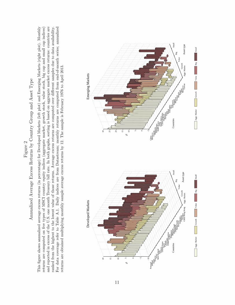
The MSCI portfolios offer a challenging cross-section of returns to explain. Figure 2

provides a pictorial description of this fact – in the figure, for each asset type, countries

are sorted according to their average market excess returns. The figure shows that

these test assets exhibit large cross-sectional variation in average aggregate equity excess

returns, across both developed and emerging countries, and across the different types

of indices.

Our two global equity factors, WMKTt+1 in U.S. dollars and LWMKTt+1 in local

currencies are monthly series, and we construct them using the daily MSCI World

Index series denominated either in U.S. dollars or in local currrencies, obtained from

Datastream. Monthly returns are computed from end-month to end-month; excess

10

Fig

ure

2A

nnual

ized

Ave

rage

Exce

ssR

eturn

sby

Cou

ntr

yG

roup

and

Ass

etT

yp

e

Th

isfi

gure

show

san

nu

aliz

edav

erag

eex

cess

retu

rns

(in

per

centa

ge)

for

Dev

elop

edM

ark

ets

(lef

tp

lot)

an

dE

mer

gin

gM

ark

ets

(rig

ht

plo

t).

Month

lyre

turn

sar

eco

mp

ute

don

five

typ

esof

MS

CI

cou

ntr

yeq

uit

yin

dic

es(a

ggre

gate

mark

et,

gro

wth

stock

,va

lue

stock

,b

igca

pan

dsm

all

cap

ind

ices

)an

dre

por

ted

inex

cess

ofth

eU

.S.

one

mon

thT

reasu

ryb

ill

rate

.In

both

gra

ph

s,so

rtin

gis

base

don

aggre

gate

mark

etex

cess

retu

rns:

cou

ntr

ies

are

ran

ked

from

the

hig

hes

tto

the

low

est

valu

eof

those

retu

rns.

Ave

rage

exce

ssre

turn

sare

com

pu

ted

over

diff

eren

tsa

mp

les

du

eto

data

avail

ab

ilit

y.F

ord

ata

cove

rage

refe

rto

Tab

leA

.1.

Dai

lyin

dic

esare

from

Data

stre

am

;m

onth

lyre

turn

sare

com

pu

ted

from

end

-of-

month

seri

es;

an

nu

ali

zed

retu

rns

are

obta

ined

mu

ltip

lyin

gm

onth

lysa

mp

leav

erage

exce

ssre

turn

sby

12.

Th

esa

mp

leis

Feb

ruary

1976

toA

pri

l2013.

Agg

r. M

arke

tG

row

th

Val

ue

Big

Sm

all

Por

tuga

l

Ir

elan

d

Japa

n

Aus

tria

Is

rael

N

ew Z

eala

nd

Ita

ly

G

reec

e

Uni

ted

Sta

tes

S

pain

Can

ada

G

erm

any

U

nite

d K

ingd

om

Fra

nce

S

inga

pore

Bel

gium

S

witz

erla

nd

D

enm

ark

N

ethe

rland

s

Nor

way

A

ustr

alia

Fin

land

S

wed

en

Chi

na H

ong

Kon

g

−10−

505

101520

Ass

et ty

pe

Dev

elop

ed M

arke

ts

Cou

ntrie

s

%

Agg

r. M

arke

tG

row

thV

alue

Big

Sm

all

Agg

r. M

arke

tG

row

th

Val

ue

Big

Sm

all

Chi

na

Mor

occo

T

aiw

an

Mal

aysi

a

P

hilip

pine

s

Sou

th K

orea

In

dia

S

outh

Afr

ica

C

zech

Rep

ublic

Tha

iland

Hun

gary

C

hile

E

gypt

C

olom

bia

Per

u

Indo

nesi

a

P

olan

d

Mex

ico

T

urke

y

Rus

sia

B

razi

l

C

hina

M

oroc

co

Tai

wan

−505

1015202530

Ass

et ty

pe

Em

ergi

ng M

arke

ts

Cou

ntrie

s

%

Agg

r. M

arke

tG

row

thV

alue

Big

Sm

all

11

returns simply subtract off the U.S. 30-day Treasury bill rate. The size, value, and

momentum international Fama and French (2012) factors and the U.S. size, value and

momentum Fama and French factors are obtained from Kenneth French’s website. All

these series are denominated in U.S. dollars. International series are available from July

1990, except for the momentum series that start in November 1990.

Our use of a world equity index built without any exchange rate data is to avoid any

misattribution of currency risk to equities and vice versa. This “synthetic” local factor

may be raise concerns about real-world implementability of our model. To address such

concerns, we show that this factor can easily be replicated using existing mutual fund

returns. The Appendix presents details about the construction of a factor mimicking

portfolio (FMP) for LWMKT , and shows that this FMP is highly correlated with

LWMKT , and delivers virtually identical returns. The Appendix also shows that the

pricing errors from estimating the model using the FMP rather than LWMKT are

virtually identical to the ones we obtain in our benchmark results.

We turn next to describing our exchange rate data.

3.2 Exchange Rates, Carry, and Dollar

We obtain daily spot and one-month forward exchange rate series (midpoint quotes)

quoted in British pounds for the same set of countries as above by merging data from

Datastream, Reuters, Barclays, and additional sources. The Online Appendix describes

these series in detail.

Assuming that the covered interest parity condition (CIP) holds, the difference

between the (log) forward and spot exchange rates (i.e., the forward discount) is equal

to the interest rate differential (in log-form) between the foreign and domestic nominal

one-month risk-free rates. Countries enter the currency data set at different points in

time according to the availability of their forward rate series. There are 15 currencies

12

at the beginning of the sample in 1976 and 28 at the end. The maximum monthly

coverage is 34, as the Euro replaces national Euro area currencies from January 1999

onwards.

Following Lustig and Verdelhan (2005, 2007), at each time t, we create six currency

portfolios by sorting all available currencies in our data set by their forward discounts.

These portfolios are rebalanced at the end of each month. The excess returns on the

carry factor in each month t, denoted Carryt, are constructed as the difference between

the returns on the top portfolio minus the return on the bottom portfolio constructed

in this fashion. The average excess return earned by a U.S. investor on the carry trade

strategy is 7.65%.

To construct the dollar excess return, we assume that in each period an investor

borrows in the U.S. and invests in all other currencies in our data set. The excess returns

on this strategy in each month are denoted by Dollart. The correlation between the

dollar factor and the carry factor has historically been low – in our data set, it is 0.18

over the full sample period, but rises to 0.40 in the post-1990 period, driven primarily

by the incidence of currency and financial crises in this latter period.

We also expand our set of test assets beyond equity markets by adding two sets of

six currency portfolios, either sorting countries by their short-term interest rates (i.e.,

Carry portfolios) or by their dollar betas (i.e., Dollar portfolios). The construction of

these portfolios is described in greater detail in Verdelhan (2014).

3.3 Mutual Fund and Hedge Fund Returns

In our empirical work, we also use our model to evaluate the exposure of international

mutual funds and hedge funds to currency risk.

Monthly mutual fund data are from CRSP. The sample includes all funds classified

as “Foreign Equity Funds” according to the CRSP fund style code. The sample period

13

is 11/1990–4/2013, that is the horizon over which the Fama-French global factors are

constructed. This choice ensures a large cross-section of mutual fund returns. At each

time t we compute returns only if CRSP provides the corresponding total net asset

value (NAV) under management.5 There are 74 funds with 5 years of past returns as

of October 1995, but up to 1148 funds by the end of the sample, which collectively

manage roughly US$ 800 billion.

Monthly hedge fund data are from the updated version of the consolidated hedge

fund database built by Ramadorai (2013) and Patton, Ramadorai and Streatfield (2013).6

The sample period for these data is 1/1994–4/2013. From this universe, we select funds

with self-reported strategies falling into “Macro” or “Emerging” categories, and we do

not select any funds-of-funds. The database includes fund returns net of management

and incentive fees, and fund assets under management (AUM).7 All series are denomi-

nated in U.S. dollars. The number of hedge funds varies over time – with 85 funds at

the beginning of the sample and 362 towards the end of the sample, which collectively

manage roughly US$ 149 billion.

We now turn to the results of our asset pricing tests.

5In the Online Appendix we compare equally-weighted and value-weighted statistics. When NAVare annual or quarterly, we linearly interpolate monthly values. We adopt the same procedure forsingle missing observations, which we interpolate using the two adjacent values. We do not interpolatereturns.

6Ramadorai (2013) and Patton, Ramadorai and Streatfield (2013) consolidate data from the TASS,HFR, CISDM, Morningstar, and BarclayHedge databases.

7In the Online Appendix we compare equally-weighted and value-weighted statistics. Single missingobservations of the AUM are linearly interpolate. We do not use interpolation for returns.

14

4 Time-series and Cross-sectional Asset Pricing Tests

4.1 Time-series Tests

As described above, there are numerous reasons to expect that capturing the role of

currency risk will require allowing for time-variation in the prices and quantities of risk.

This importance of using a conditional model is also consistent with the findings of

Dumas and Solnik (1995) when testing international asset pricing models.

Harvey (1991) and Dumas and Solnik (1995) capture time-variation in factor risk

premia by conditioning on a set of instruments. As Cochrane (2001) notes, since the

econometrician does not know the true set of state variables, conditional asset pricing

tests are joint tests of the set of variables employed as conditioning information and

whether the asset pricing model minimizes pricing errors.

Our principal approach in our asset pricing tests, therefore, is to estimate time-

variation in factor loadings using simple rolling window regressions in the spirit of

Lewellen and Nagel (2006). Following their implementation, we use 60-month rolling

windows for our regressions. This choice means that the maximum number of rolling

regressions we run for a single country is 388, and the minimum is 161 – this variation

is a result of country-specific data availability. In the Online Appendix, we verify

that our results are robust to the use of other window sizes (namely, 48- and 72-month

windows).8

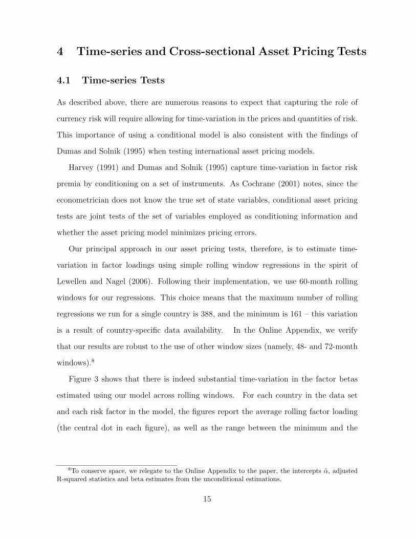
Figure 3 shows that there is indeed substantial time-variation in the factor betas

estimated using our model across rolling windows. For each country in the data set

and each risk factor in the model, the figures report the average rolling factor loading

(the central dot in each figure), as well as the range between the minimum and the

8To conserve space, we relegate to the Online Appendix to the paper, the intercepts α, adjustedR-squared statistics and beta estimates from the unconditional estimations.

15

maximum estimated rolling factor loadings (the two ends of the line in each figure).9

Across countries, especially for the currency factors, there are significant differences

both in the magnitude of the risk exposures, and the degree to which they vary over

time. While these features are evident in both sets of markets, they are more pronounced

in emerging markets.

With few exceptions (primarily in developed countries), estimated carry loadings

switch sign over time, and dollar betas are more volatile than carry betas. Extreme

examples of time variation include the dollar loadings of Indonesia, and the carry load-

ings of Turkey. The Netherlands and the United States show the most stable exposures

to currency risk. The heterogeneity across countries is so pronounced that it is difficult

to identify common patterns. For example, while Japan and Switzerland are typical

carry-trade funding countries, the carry factor loadings of their equity returns often

move in opposite directions.

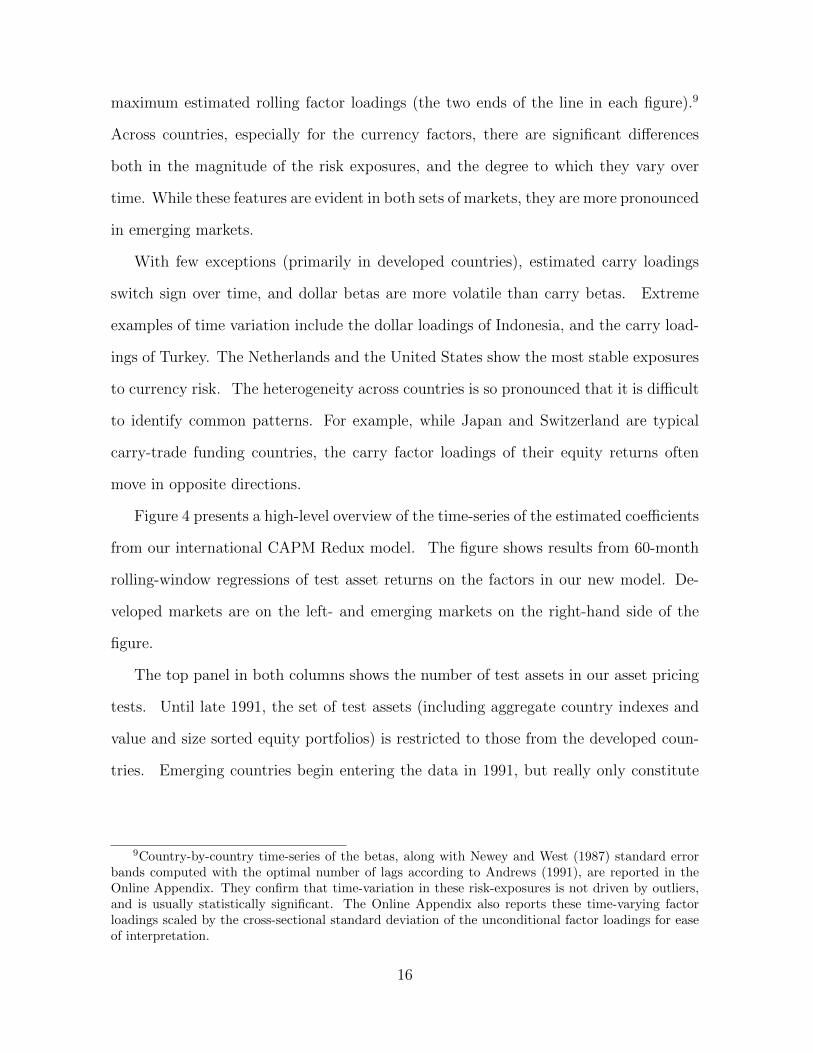
Figure 4 presents a high-level overview of the time-series of the estimated coefficients

from our international CAPM Redux model. The figure shows results from 60-month

rolling-window regressions of test asset returns on the factors in our new model. De-

veloped markets are on the left- and emerging markets on the right-hand side of the

figure.

The top panel in both columns shows the number of test assets in our asset pricing

tests. Until late 1991, the set of test assets (including aggregate country indexes and

value and size sorted equity portfolios) is restricted to those from the developed coun-

tries. Emerging countries begin entering the data in 1991, but really only constitute

9Country-by-country time-series of the betas, along with Newey and West (1987) standard errorbands computed with the optimal number of lags according to Andrews (1991), are reported in theOnline Appendix. They confirm that time-variation in these risk-exposures is not driven by outliers,and is usually statistically significant. The Online Appendix also reports these time-varying factorloadings scaled by the cross-sectional standard deviation of the unconditional factor loadings for easeof interpretation.

16

Fig

ure

3T

ime-

Var

yin

gF

acto

rB

etas

Th

isfigu

resh

ows,

for

each

cou

ntr

yin

the

data

set,

the

inte

rval

bet

wee

nth

em

inim

um

an

dth

em

axim

um

valu

e(b

lack

arr

ow)

of

ati

me-

seri

esof

60-m

onth

roll

ing

fact

orb

etas

alon

gw

ith

thei

rav

erage

valu

es(w

hit

ed

ot)

.M

onth

lyeq

uit

yex

cess

retu

rns

are

regre

ssed

on

aco

nst

ant,

the

glo

bal

equ

ity

fact

or(L

WM

KT

)an

dth

ed

olla

ran

dca

rry

fact

or

over

60-m

onth

roll

ing

win

dow

s.T

est

ass

ets

are

exce

ssre

turn

son

MS

CI

aggre

gate

mark

etin

dic

esd

enom

inat

edin

U.S

.d

olla

rs.

The

sam

ple

per

iod

isF

ebru

ary

1976

toA

pri

l2013.

−4

−2

02

46

Tur

key

Tha

iland

Tai

wan

Sou

th K

orea

Sou

th A

fric

aR

ussi

aP

olan

dP

hilip

pine

sP

eru

Mor

occo

Mex

ico

Mal

aysi

aIn

done

sia

Indi

aH

unga

ryE

gypt

Cze

ch R

epub

licC

olom

bia

Chi

naC

hile

Bra

zil

Uni

ted

Sta

tes

Uni

ted

Kin

gdom

Sw

itzer

land

Sw

eden

Spa

inS

inga

pore

Por

tuga

lN

orw

ayN

ew Z

eala

ndN

ethe

rland

sJa

pan

Italy

Isra

elIr

elan

dH

ong

Kon

gG

reec

eG

erm

any

Fra

nce

Fin

land

Den

mar

kC

anad

aB

elgi

umA

ustr

iaA

ustr

alia

β LWM

KT

Exp

osur

e to

LW

MK

T

−4

−2

02

46

β Dol

lar

Exp

osur

e to

Dol

lar

Ave

rage

−4

−2

02

46

β Car

ry

Exp

osur

e to

Car

ry

Min

/Max

17

Figure 4CAPM Redux: Significant Time-Varying Exposure to Global Factors

This figure reports the time-series of the share of test assets with significant exposure to the globalequity and currency factors (β∗∗t ). Monthly equity excess returns are regressed on a constant and theglobal equity, dollar and carry factor over 60-month rolling windows. The size of the cross-sectionvaries across time according to data coverage (# Test Assets). Test assets are equity excess returns onMSCI aggregate market, value, growth, small cap and big cap indices for developed (left graphs) andemerging (right graphs) markets. Standard errors are Newey-West. Statistical significance is tested atthe 5% level. The sample period is February 1976 to April 2013.

Developed Markets Emerging Markets

Jan81 May86 Sep91 Feb97 Jul02 Nov07 Apr130

40

80

120 # Test Assets

Jan81 May86 Sep91 Feb97 Jul02 Nov07 Apr130

40

80

120 # Test Assets

Jan81 May86 Sep91 Feb97 Jul02 Nov07 Apr130

25

50

75

100

%

βt, LWMKT**

Jan81 May86 Sep91 Feb97 Jul02 Nov07 Apr130

25

50

75

100

%

βt, LWMKT**

Jan81 May86 Sep91 Feb97 Jul02 Nov07 Apr130

25

50

75

100

%

βt, Dollar**

Jan81 May86 Sep91 Feb97 Jul02 Nov07 Apr130

25

50

75

100

%

βt, Dollar**

Jan81 May86 Sep91 Feb97 Jul02 Nov07 Apr130

25

50

75

100

%

βt, Carry**

Jan81 May86 Sep91 Feb97 Jul02 Nov07 Apr130

25

50

75

100

%

βt, Carry**

18

a significant fraction of the data from the late 1990s onwards. The set of assets con-

tinues expanding well into the 2000s, posing some challenges for time-series tests, since

we suffer from large N , small T problems in our unbalanced panel. We explain how

we conduct GRS tests in this setting below.

The panels below show the percentage of betas from the model that are statistically

significant in each rolling window. Despite the overlap between these windows and the

mechanical persistence of these estimates over shorter periods, it is clear that there is

considerable time-variation in the statistical significance of these beta estimates. The

equity factor, LWMKT is virtually always significant for the developed markets, and

by the end of the sample period, for the emerging markets as well. The Dollar factor

also shows considerable statistical significance for the developed markets, with over

50% of the set of test assets having statistically significant loadings on this factor,

and has increasing significance as an explanatory variable for emerging market assets,

reaching statistical significance in 75% of test asset regressions by the end of the sample.

Finally, the Carry factor shows substantial time variation in its statistical significance,

peaking after crises, with statistical significance seen for between 10% and 50% of test

assets depending on the rolling window. The fact that these factors are statistically

significant is important, especially in light of recent literature in asset pricing which

casts doubt on second-stage results from standard two-pass cross-sectional asset pricing

tests when first-stage betas are statistically insignificant (see, for example, Bryzgalova,

2015).

Table 1 shows the first comparison between our model and the competitor inter-

national asset pricing models, using the usual “GRS” F -test of Gibbons, Ross,and

Shanken (1989) on each model to test whether all test-asset intercepts are jointly zero.

The table compares the models by reporting the share of rolling windows in which the

GRS test rejects the null hypothesis that rolling alphas implied by a given asset pricing

model are jointly zero, at the 5% level. To combat the “large N , small T” issue, we re-

19

Table 1Horse-Race: % Of Rolling GRS Tests Rejecting The Null

This table compares the World CAPM, the International CAPM, the Fama-French four-factor model(4FF) and the CAPM Redux by reporting the share of rolling windows in which the GRS test rejects thenull hypothesis that rolling alphas implied by a given asset pricing model are jointly zero at the 5% level.Intercepts are estimated by regressing country-i equity excess returns on a constant and the appropriateset of factors over rolling-windows of 60 months. Under the assumption of normality, the GRS test

statistic is F-distributed and defined as T−N−KN

(1 + ET (f)′Ω−1ET (f)

)−1

α′Σ−1α ∼ F(N,T−N−K),

where T, N and K denote the sample size, the number of test assets, and the number of factors,respectively, Ω is the variance-covariance matrix of the factors f and Σ is the variance-covariancematrix of the estimated residuals. Five sets of test assets are considered (i.e., excess returns onMSCI aggregate market/value/growth indices and small/large capitalization indices). Developed andemerging markets are treated separately in Panel I and II and jointly in Panel III. Fama-French factorsare obtained by combining U.S. factors with their global counterparts. The sample period is February1976 to April 2013.

Model Test assets

Aggr. Market Value Growth Small Big

I: Developed Markets

World CAPM 28.68 3.62 1.29 4.91 1.81

Int. CAPM 29.72 4.91 0.26 4.91 1.03

4FF 6.20 2.07 4.65 0.00 4.13

CAPM Redux 8.01 2.58 1.81 2.84 2.33

II: Emerging Markets

World CAPM 10.59 3.88 5.17 3.36 3.10

Int. CAPM 10.34 0.78 2.84 5.43 3.10

4FF 3.88 2.58 0.00 2.07 3.10

CAPM Redux 6.72 0.00 0.26 1.03 5.68

III: All Markets

World CAPM 11.89 1.03 2.07 6.46 3.62

Int. CAPM 17.31 2.84 1.81 6.72 2.33

4FF 2.07 2.07 2.84 3.10 4.39

CAPM Redux 5.43 0.00 2.58 5.17 1.29

20

port this fraction separately for each category of test assets, i.e., the country indexes, as

well as all value, growth, small, and big stock portfolios across developed and emerging

markets, as well as for all markets together.

The table shows that our model exhibits far lower fractions of rejections of the GRS

null than the World CAPM and the International CAPM, especially when applied

to the country indexes. Interestingly, this outperformance of our model in the time

series domain is particularly pronounced for the developed markets rather than for

the emerging markets. The Fama-French-Carhart four factor model has performance

comparable to that of our model across both emerging and developed markets, but for

the set of Value test assets, our model generally beats even this model, despite the

fact that the Fama-French model was first constructed to explain the value and size

premiums.

Using the time-series estimates of factor betas, we turn to the factor risk premiums

in the cross-section of test asset returns.

4.2 Cross-sectional Tests

As a preliminary exercise, Figure 5 provides a pictorial representation of the relative

performance of the models in the cross-section. The vertical axis in these plots is

common to all models, and reports the realized average excess returns (in percentage)

of our entire cross-section of test assets over the full sample period. The horizontal

axis reports the average excess returns of the same test assets as predicted by each

model, and varies across the four models we inspect. For the purposes of these plots,

we compute predicted returns by using the factor loadings for each asset estimated using

the 60-month rolling windows described above. We then multiply these estimated factor

loadings by factor means computed over the same time window, and average these

conditional predictions across all periods. As usual, better performing models will

21

generate points which lie close to the 45line, and deviations from this line indicate

pricing errors.

The figure shows that the World CAPM and the International CAPM underestimate

realized average excess returns: the large cross-sectional variation observed in the data

is not matched because there is little cross-sectional variation in the predictions of these

models, leading to a more vertical line. From the figure it is apparent that this poor

performance is not driven by a particular type of equity asset; the differences between

predictions and realizations are similar for the various different types of assets. The

Fama-French-Carhart four-factor model does do substantially better than the more

theoretically grounded models, but there is still significant deviation from the 45line.

Our model significantly improves the visual relationship between predicted and real-

ized average returns. These improvements come from two sources. First, we explicitly

model the currency component embedded in foreign equity market returns. Second,

we reduce the noise in measured currency risks by relying on two global currency risk

factors rather than a selected few currency excess returns.

We confirm this result in a number of ways in the Online Appendix. First, we

find that the cross-sectional average R2 from these time-series regressions is generally

higher for our model than for the competition. At each date in the sample, the

global equity, dollar, and carry factors explain a larger share of the time-series variation

in international equity returns than the world CAPM. We also find that our model

outperforms the International CAPM as we move from the distant past towards the

recent past. This latter finding suggests that the increasing integration of global markets

might account for the increasing explanatory power of global currency factors.

Next, we relax the no-arbitrage condition that pins down the market prices of risk

and estimate them using the cross-section of excess returns. We conduct our cross-

sectional tests using the standard two-pass cross-sectional approach of Fama and Mac-

Beth (1973, henceforth FMB). For each of the models in our comparisons, we run FMB

22

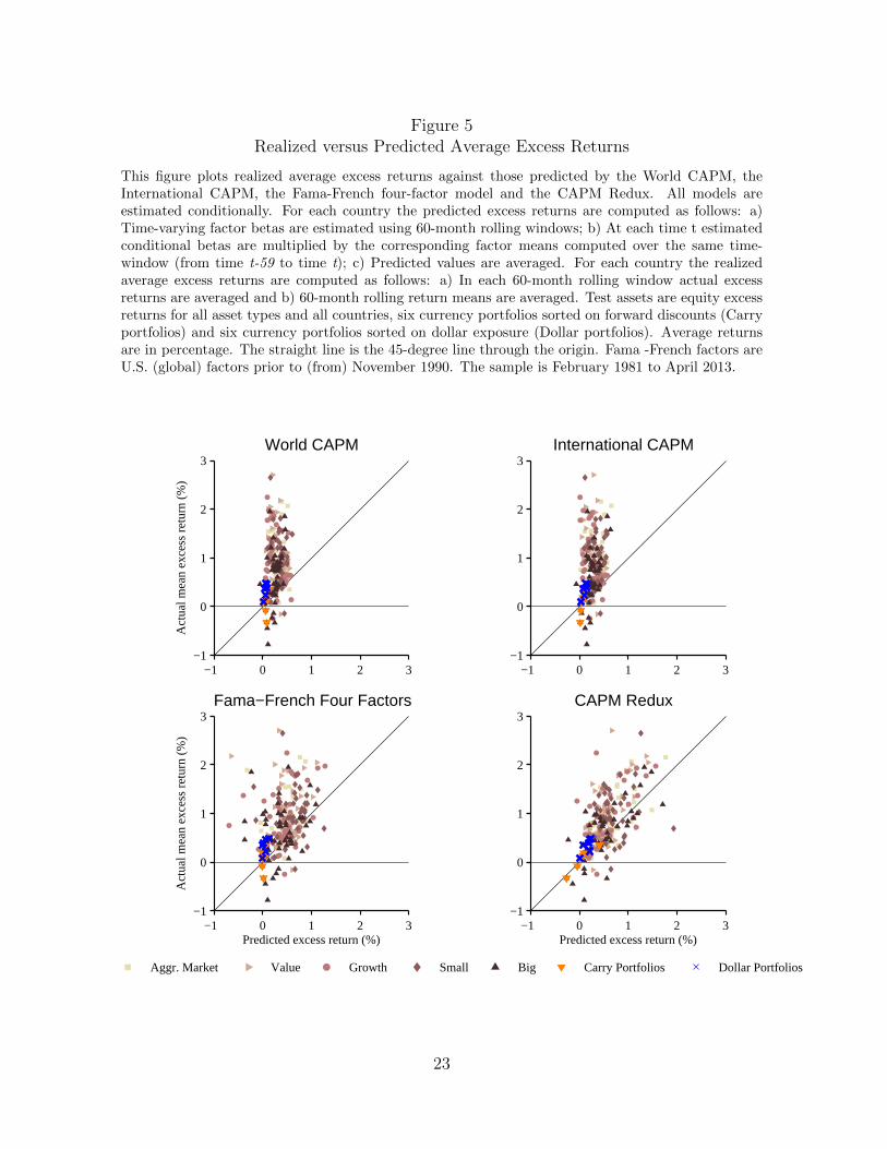
Figure 5Realized versus Predicted Average Excess Returns

This figure plots realized average excess returns against those predicted by the World CAPM, theInternational CAPM, the Fama-French four-factor model and the CAPM Redux. All models areestimated conditionally. For each country the predicted excess returns are computed as follows: a)Time-varying factor betas are estimated using 60-month rolling windows; b) At each time t estimatedconditional betas are multiplied by the corresponding factor means computed over the same time-window (from time t-59 to time t); c) Predicted values are averaged. For each country the realizedaverage excess returns are computed as follows: a) In each 60-month rolling window actual excessreturns are averaged and b) 60-month rolling return means are averaged. Test assets are equity excessreturns for all asset types and all countries, six currency portfolios sorted on forward discounts (Carryportfolios) and six currency portfolios sorted on dollar exposure (Dollar portfolios). Average returnsare in percentage. The straight line is the 45-degree line through the origin. Fama -French factors areU.S. (global) factors prior to (from) November 1990. The sample is February 1981 to April 2013.

−1 0 1 2 3−1

0

1

2

3 World CAPM

Act

ual m

ean

exce

ss r

etur

n (%

)

−1 0 1 2 3−1

0

1

2

3 International CAPM

−1 0 1 2 3−1

0

1

2

3Fama−French Four Factors

Act

ual m

ean

exce

ss r

etur

n (%

)

Predicted excess return (%)−1 0 1 2 3

−1

0

1

2

3 CAPM Redux

Predicted excess return (%)

Aggr. Market Value Growth Small Big Carry Portfolios Dollar Portfolios

23

tests in three different ways. In the first variant of these FMB tests (which we denote as

FMB1), we estimate the factor loadings using unconditional time-series regressions over

the full sample. We then compute market prices of risk (λ) via a cross-sectional regres-

sion of average excess returns of the test assets on these unconditional factor loadings.

In the second variant (which we denote FMB2), first-stage betas continue to be obtained

using unconditional time-series regressions over the full sample as in FMB1. However,

in the second stage, we run T cross-sectional regressions, one for each time period, of

country excess returns on these estimated factor loadings. The average market prices of

risk are then computed as simple averages of the slope coefficients obtained from these

T cross-sectional regressions. In the third variant (denoted FMBTV ), we obtain time-

varying factor loadings using our rolling regressions over 60-month windows. In each

period t+ 1, we estimate market prices of risk λt+1 using cross-sectional regressions of

test asset returns on these time-varying factor loadings estimated using windows ending

in period t. Average market prices of risk are once again simple averages of λt+1 over

all periods T . In all three variants of these tests, we omit constants in the second

stage of the FMB procedure. To ensure that the three tests are comparable, the FMB1

and FMB2 tests are carried out on the second-stage estimation sample of the FMBTV

procedure.

Table 2 reports the estimates of the average market prices of risk along with Shanken

(1992)-corrected standard errors (in parentheses) from these tests across models which

are in blocks of rows. The columns identify the set of test assets on which we run these

tests. The first set of test assets includes aggregate market excess returns, and value

and size-sorted portfolios for the developed markets in the sample (120 assets), as well

as 12 currency portfolios. The second set of test assets expands the equity cross-section

to include assets from emerging markets, leading to a total of 225 equity assets plus 12

currency portfolios.

The table shows that across all model specifications, cross-sections of test assets,

24

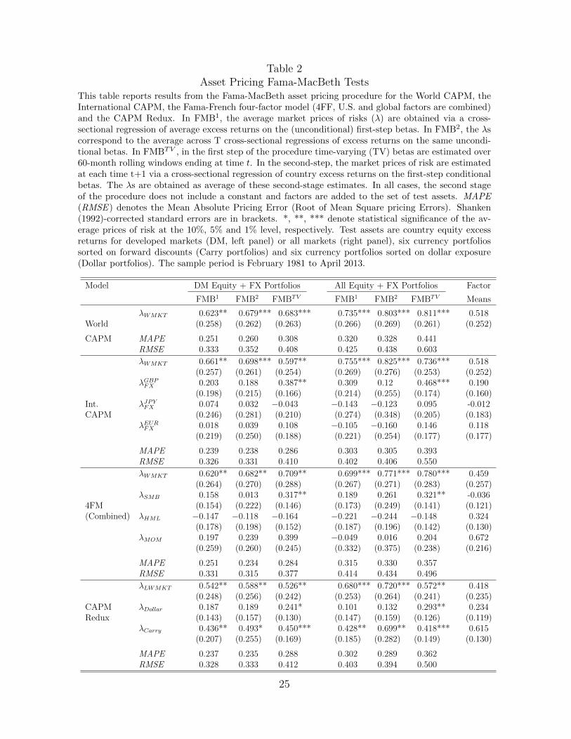
Table 2Asset Pricing Fama-MacBeth Tests

This table reports results from the Fama-MacBeth asset pricing procedure for the World CAPM, theInternational CAPM, the Fama-French four-factor model (4FF, U.S. and global factors are combined)and the CAPM Redux. In FMB1, the average market prices of risks (λ) are obtained via a cross-sectional regression of average excess returns on the (unconditional) first-step betas. In FMB2, the λscorrespond to the average across T cross-sectional regressions of excess returns on the same uncondi-tional betas. In FMBTV , in the first step of the procedure time-varying (TV) betas are estimated over60-month rolling windows ending at time t. In the second-step, the market prices of risk are estimatedat each time t+1 via a cross-sectional regression of country excess returns on the first-step conditionalbetas. The λs are obtained as average of these second-stage estimates. In all cases, the second stageof the procedure does not include a constant and factors are added to the set of test assets. MAPE(RMSE ) denotes the Mean Absolute Pricing Error (Root of Mean Square pricing Errors). Shanken(1992)-corrected standard errors are in brackets. *, **, *** denote statistical significance of the av-erage prices of risk at the 10%, 5% and 1% level, respectively. Test assets are country equity excessreturns for developed markets (DM, left panel) or all markets (right panel), six currency portfoliossorted on forward discounts (Carry portfolios) and six currency portfolios sorted on dollar exposure(Dollar portfolios). The sample period is February 1981 to April 2013.

Model DM Equity + FX Portfolios All Equity + FX Portfolios Factor

FMB1 FMB2 FMBTV FMB1 FMB2 FMBTV Means

λWMKT 0.623** 0.679*** 0.683*** 0.735*** 0.803*** 0.811*** 0.518World (0.258) (0.262) (0.263) (0.266) (0.269) (0.261) (0.252)

CAPM MAPE 0.251 0.260 0.308 0.320 0.328 0.441RMSE 0.333 0.352 0.408 0.425 0.438 0.603

λWMKT 0.661** 0.698*** 0.597** 0.755*** 0.825*** 0.736*** 0.518(0.257) (0.261) (0.254) (0.269) (0.276) (0.253) (0.252)

λGBPFX 0.203 0.188 0.387** 0.309 0.12 0.468*** 0.190(0.198) (0.215) (0.166) (0.214) (0.255) (0.174) (0.160)

Int. λJPYFX 0.074 0.032 −0.043 −0.143 −0.123 0.095 -0.012CAPM (0.246) (0.281) (0.210) (0.274) (0.348) (0.205) (0.183)

λEURFX 0.018 0.039 0.108 −0.105 −0.160 0.146 0.118(0.219) (0.250) (0.188) (0.221) (0.254) (0.177) (0.177)

MAPE 0.239 0.238 0.286 0.303 0.305 0.393RMSE 0.326 0.331 0.410 0.402 0.406 0.550

λWMKT 0.620** 0.682** 0.709** 0.699*** 0.771*** 0.780*** 0.459(0.264) (0.270) (0.288) (0.267) (0.271) (0.283) (0.257)

λSMB 0.158 0.013 0.317** 0.189 0.261 0.321** -0.0364FM (0.154) (0.222) (0.146) (0.173) (0.249) (0.141) (0.121)(Combined) λHML −0.147 −0.118 −0.164 −0.221 −0.244 −0.148 0.324

(0.178) (0.198) (0.152) (0.187) (0.196) (0.142) (0.130)λMOM 0.197 0.239 0.399 −0.049 0.016 0.204 0.672

(0.259) (0.260) (0.245) (0.332) (0.375) (0.238) (0.216)

MAPE 0.251 0.234 0.284 0.315 0.330 0.357RMSE 0.331 0.315 0.377 0.414 0.434 0.496

λLWMKT 0.542** 0.588** 0.526** 0.680*** 0.720*** 0.572** 0.418(0.248) (0.256) (0.242) (0.253) (0.264) (0.241) (0.235)

CAPM λDollar 0.187 0.189 0.241* 0.101 0.132 0.293** 0.234Redux (0.143) (0.157) (0.130) (0.147) (0.159) (0.126) (0.119)

λCarry 0.436** 0.493* 0.450*** 0.428** 0.699** 0.418*** 0.615(0.207) (0.255) (0.169) (0.185) (0.282) (0.149) (0.130)

MAPE 0.237 0.235 0.288 0.302 0.289 0.362RMSE 0.328 0.333 0.412 0.403 0.394 0.500

25

and testing approaches, the world equity factor is priced, whether it is measured in local

currency or U.S. dollar terms. The statistical significance of this result holds at the five

percent level or better. This finding supports the early evidence in the international

finance literature that international investors are compensated for taking on risk that

is correlated with returns on the world equity market portfolio.

In contrast, there is little evidence to support the pricing of currency risk in models

other than our own. Looking across the three currencies included in the International

CAPM, only the British pound appears to carry a significant currency premium in our

sample. Moreover, this result holds only when time-variation is taken into account

(FMBTV ). The importance of using a conditional model is consistent with the findings

of Dumas and Solnik (1995), however even allowing for time-variation in factor loadings

and risk premia, the German mark/Euro and Japanese Yen are not priced over the

sample period for the wider cross-section of assets. This result is potentially attributable

to the longer sample period, the larger cross-section of test assets, and our use of a

methodology based on rolling windows instead of instrumental variables to model time-

variation.

The table also shows that there is no statistical evidence for a value or momentum

premium in the cross-section of test assets, either conditionally or unconditionally.

However there is some evidence to support the existence of a size premium, especially

when we evaluate the Fama-French model allowing for time-variation in factor loadings.

In contrast with these results, we find evidence to support the pricing of currency

risk when we measure this risk using the dollar and carry factors. This is even true to

some extent unconditionally, in the sense that the carry factor is priced using FMB1

across developed and developed plus emerging cross-sections, and using FMB2 in the

broader developed plus emerging cross-section.

The results supporting our model become substantially stronger when we account

for time-variation in factor loadings as well as in risk premia, using FMBTV . The prices

26

of dollar and carry risk are all significantly different from zero at the 5% level or better,

in both cross-sections.

Additional evidence on the models is provided when we inspect the prices of risk of

the equity, dollar, and carry factors and compare them with the average excess returns

of those factors which are provided in the final column of Table 2. The no-arbitrage

condition implies, since the beta of each factor on itself is obviously one, that the

market price of risk of each factor should be equal to the average of the factor. While

the sample is short, leading to difficulties in estimating this relationship precisely, we

do see that these factor means are relatively close to the estimated factor risk premia.

For the other models, the price of equity risk is much higher, further removed from its

sample mean. As noted, however, the sample is indeed short, leading to substantial

imprecision, and susceptibility to Daniel and Titman’s (1997) critique. We cannot

of course rule out a characteristics-based behavioral explanation of the cross-sectional

variation in test asset returns.

For each model, Table 2 also reports the cross-sectional Mean Absolute Pricing Error

(MAPE) and the cross-sectional Root Mean Square Error (RMSE). Consistent with the

evidence discussed above, our factor model delivers relatively smaller RMSEs than the

competition, although these differences are not substantial.

The Online Appendix reports a number of additional robustness checks including

re-estimating the model on samples of expanding sizes, either moving forwards in time,

beginning in 2/1976 or moving backwards in time, beginning in 12/2013. The dollar

and carry factors appear priced even in samples that exclude the recent financial crisis

(i.e., before 2007). Small perturbations in the estimation sample do not imply abrupt

changes in the estimates. The magnitude of these currency premia vary smoothly over

time suggesting that the price of risk (not merely risk exposure) is time-varying. We

also find that the significance of the pricing results for the model increases over time.

This pattern is certainly related to the increase in power arising from a broader cross-

27

section of asset returns available to test the model, as well as the increasing global

capital market integration over time.

One obvious question is whether our strong results are simply a consequence of the

currency return component embedded in dollar-denominated test asset returns, and the

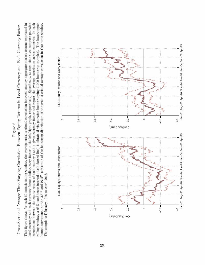
pricing of these currency components by the carry and dollar factors. Figure 6 shows

that a simple story of this nature would be insufficient to explain the somewhat involved

dynamics of equity and currency risk.

28

Fig

ure

6C

ross

-Sec

tion

alA

vera

geT

ime-

Var

yin

gC

orre

lati

onB

etw

een

Equit

yR

eturn

sin

Loca

lC

urr

ency

and

Eac

hC

urr

ency

Fac

tor

Th

isfi

gure

show

s,fo

rea

ch60

-mon

thro

llin

gw

ind

ow,

the

aver

age

cross

-sec

tion

al

corr

elati

on

bet

wee

nco

untr

yaggre

gate

mark

etre

turn

sex

pre

ssed

inlo

cal

curr

ency

and

each

curr

ency

fact

or(d

olla

r/ca

rry

fact

or

inth

ele

ft/ri

ght

gra

ph

,re

spec

tive

ly).

Sp

ecifi

call

y,at

each

tim

et

we

com

pu

tep

air

wis

eco

rrel

atio

ns

bet

wee

nth

eeq

uit

yre

turn

ofea

chco

untr

y-i

an

da

giv

encu

rren

cyfa

ctor

an

dre

port

the

aver

age

corr

elati

on

acr

oss

cou

ntr

ies.

Inea

chro

llin

gw

ind

ow,

a95

%co

nfi

den

cein

terv

al(d

ash

-dott

edli

ne)

isob

tain

edvia

pair

wis

eb

oots

trap

pin

g(1

000

boots

trap

sam

ple

s).

Th

elo

wer

/u

pp

erb

oun

dco

rres

pon

ds

toth

e2.

5th

and

97.5

thp

erce

nti

leof

the

boots

trap

dis

trib

uti

on

of

the

cross

-sec

tion

al

aver

age

corr

elati

on

inth

at

tim

e-w

ind

ow.

Th

esa

mp

leis

Feb

ruar

y19

76to

Ap

ril

2013

.

Jan−

81A

ug−

85A

pr−

90N

ov−

94Ju

n−99

Jan−

04S

ep−

08A

pr−

13

−0.

4

−0.

20

0.2

0.4

0.6

0.81

LOC

Equ

ity R

etur

ns a

nd D

olla

r fa

ctor

Corr(Ret, Dollar)t

Jan−

81A

ug−

85A

pr−

90N

ov−

94Ju

n−99

Jan−

04S

ep−

08A

pr−

13

−0.

4

−0.

20

0.2

0.4

0.6

0.81

LOC

Equ

ity R

etur

ns a

nd C

arry

fact

or

Corr(Ret, Carry)t

29

The figure reports the cross-sectional average correlation coefficient between coun-

try aggregate market equity returns expressed in local currency and the dollar factor

(left panel) and the carry factor (right panel). Clearly, equity and currency risk are

not orthogonal to one another, and demonstrate significant time-variation in their rela-

tionship. Particularly over the second half of the sample period that we consider, these

correlations are significant and increasing, sometimes non-linearly. These correlations

reach 60% (50%) at the end of our sample period for the dollar (carry) factor. We

discuss this issue in more detail when we present the model in the next section.

Next, we show that a large proportion of mutual and hedge funds investing inter-

nationally are also exposed to currency risk, which we are well able to detect using our

model.

4.3 Global Risk in Mutual and Hedge Fund Returns

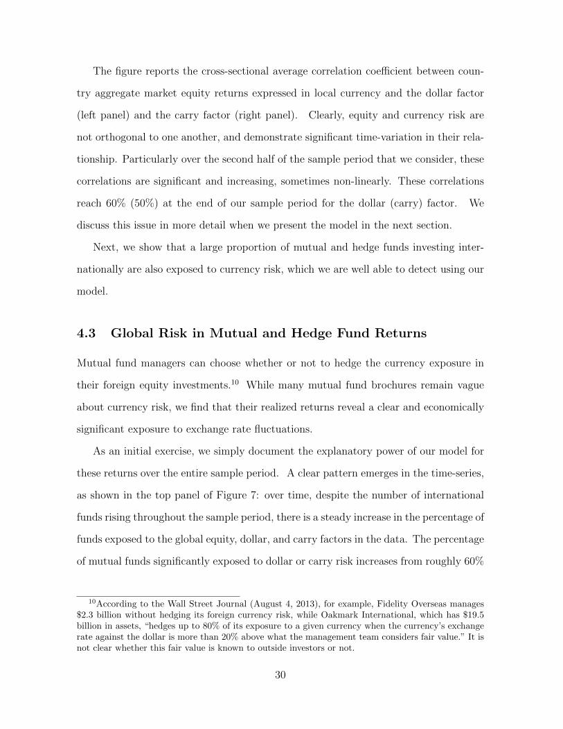
Mutual fund managers can choose whether or not to hedge the currency exposure in

their foreign equity investments.10 While many mutual fund brochures remain vague

about currency risk, we find that their realized returns reveal a clear and economically

significant exposure to exchange rate fluctuations.

As an initial exercise, we simply document the explanatory power of our model for

these returns over the entire sample period. A clear pattern emerges in the time-series,

as shown in the top panel of Figure 7: over time, despite the number of international

funds rising throughout the sample period, there is a steady increase in the percentage of

funds exposed to the global equity, dollar, and carry factors in the data. The percentage

of mutual funds significantly exposed to dollar or carry risk increases from roughly 60%

10According to the Wall Street Journal (August 4, 2013), for example, Fidelity Overseas manages$2.3 billion without hedging its foreign currency risk, while Oakmark International, which has $19.5billion in assets, “hedges up to 80% of its exposure to a given currency when the currency’s exchangerate against the dollar is more than 20% above what the management team considers fair value.” It isnot clear whether this fair value is known to outside investors or not.

30

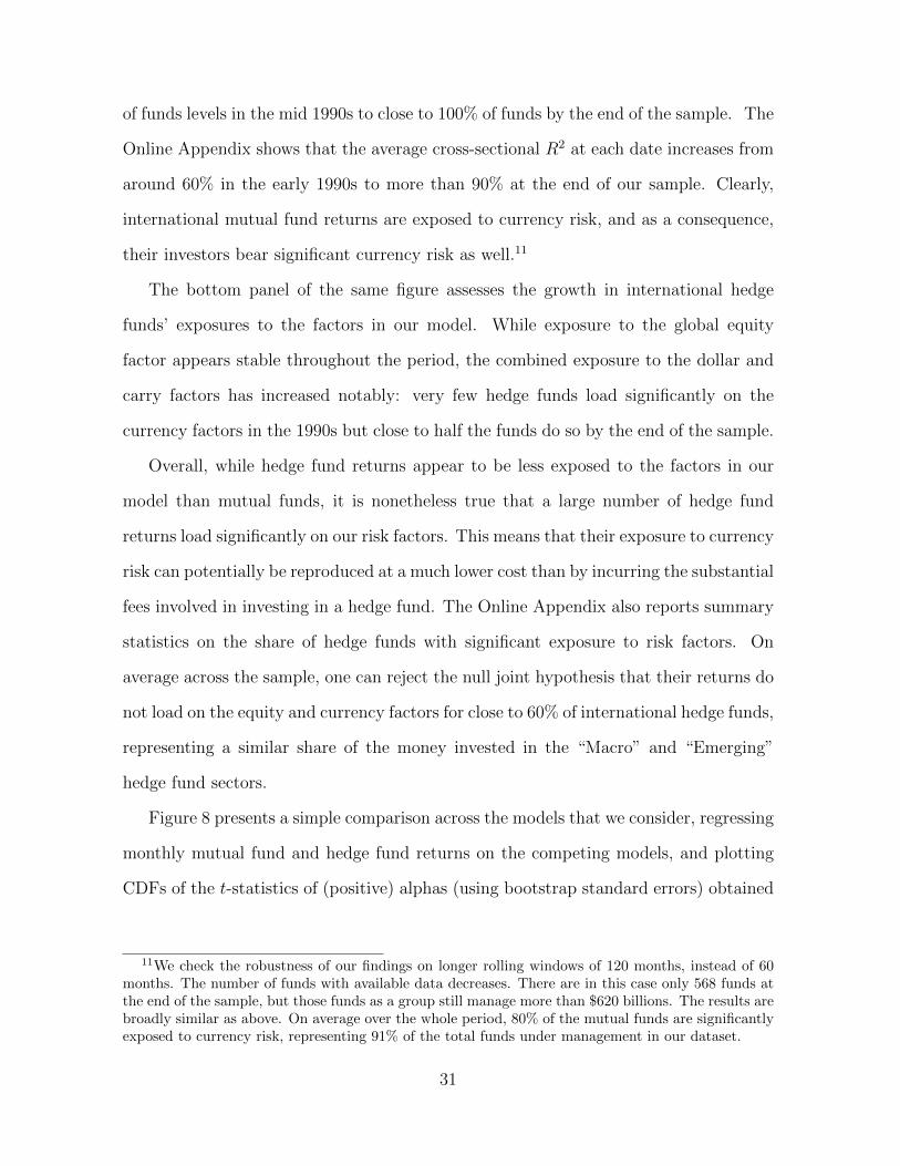
of funds levels in the mid 1990s to close to 100% of funds by the end of the sample. The

Online Appendix shows that the average cross-sectional R2 at each date increases from

around 60% in the early 1990s to more than 90% at the end of our sample. Clearly,

international mutual fund returns are exposed to currency risk, and as a consequence,

their investors bear significant currency risk as well.11

The bottom panel of the same figure assesses the growth in international hedge

funds’ exposures to the factors in our model. While exposure to the global equity

factor appears stable throughout the period, the combined exposure to the dollar and

carry factors has increased notably: very few hedge funds load significantly on the

currency factors in the 1990s but close to half the funds do so by the end of the sample.

Overall, while hedge fund returns appear to be less exposed to the factors in our

model than mutual funds, it is nonetheless true that a large number of hedge fund

returns load significantly on our risk factors. This means that their exposure to currency

risk can potentially be reproduced at a much lower cost than by incurring the substantial

fees involved in investing in a hedge fund. The Online Appendix also reports summary

statistics on the share of hedge funds with significant exposure to risk factors. On

average across the sample, one can reject the null joint hypothesis that their returns do

not load on the equity and currency factors for close to 60% of international hedge funds,

representing a similar share of the money invested in the “Macro” and “Emerging”

hedge fund sectors.

Figure 8 presents a simple comparison across the models that we consider, regressing

monthly mutual fund and hedge fund returns on the competing models, and plotting

CDFs of the t-statistics of (positive) alphas (using bootstrap standard errors) obtained

11We check the robustness of our findings on longer rolling windows of 120 months, instead of 60months. The number of funds with available data decreases. There are in this case only 568 funds atthe end of the sample, but those funds as a group still manage more than $620 billions. The results arebroadly similar as above. On average over the whole period, 80% of the mutual funds are significantlyexposed to currency risk, representing 91% of the total funds under management in our dataset.

31

Figure 7Mutual Funds’ and Hedge Funds’ Significant Exposure to Global Factors

This figure plots the time-series of the share of hedge funds (top three graphs) and mutual funds(bottom three graphs) with significant exposure to the CAPM Redux factors (LWMKT, Dollar andCarry). At each point in time monthly hedge fund/mutual fund returns are regressed on a constantand the three global factors over rolling-windows of 60 months. The first and fourth panels report thenumber of funds with available data. The second and fifth panels report the percentage of funds withsignificance exposure to LWMKT at the 5% significance level (i.e., t-statistic on the equity factor above1.96 in absolute value). Standard errors are obtained via bootstrapping (1000 bootstrap samples). Thethird and last panel report the percentage of funds with significance exposure to both the dollar and thecarry factor at the 5% significance level (i.e. p-value of the F -test below 5% under the null hypothesisthat both FX loadings are zero). Funds are equally-weighted. Hedge fund data are from the updatedversion of the consolidated hedge fund database by Ramadorai (2013) and Patton, Ramadorai andStreatfield (2013). The sample includes all funds classified as “Macro” or “Emerging” according to thestrategy code. The sample period is January 1994 to April 2013. The mutual fund sample includes allfunds classified as “Foreign Equity Funds” according to the CRSP fund style code. The sample periodis November 1990 to April 2013. All data are monthly.

1996 1998 2000 2002 2004 2006 2008 2010 2012

0

600

1200

Num

ber

of fu

nds

Mutual Funds

1996 1998 2000 2002 2004 2006 2008 2010 2012

0

0.5

1

Equ

ityF

acto

r

1996 1998 2000 2002 2004 2006 2008 2010 2012

0

0.5

1

Cur

renc

yF

acto

rs

1996 1998 2000 2002 2004 2006 2008 2010 2012

0

200

400

Num

ber

of fu

nds

Hedge Funds

1996 1998 2000 2002 2004 2006 2008 2010 2012

0

0.5

1

Equ

ityF

acto

r

1996 1998 2000 2002 2004 2006 2008 2010 2012

0

0.5

1

Cur

renc

yF

acto

rs

32

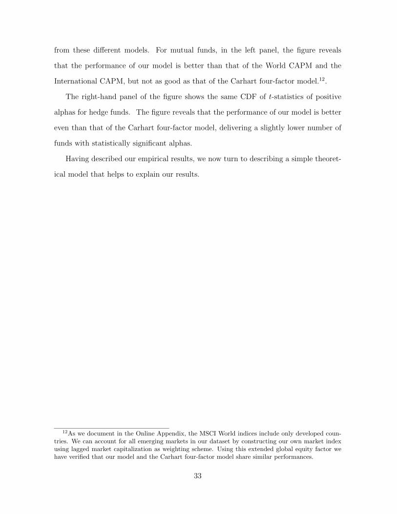
from these different models. For mutual funds, in the left panel, the figure reveals

that the performance of our model is better than that of the World CAPM and the

International CAPM, but not as good as that of the Carhart four-factor model.12.

The right-hand panel of the figure shows the same CDF of t-statistics of positive

alphas for hedge funds. The figure reveals that the performance of our model is better

even than that of the Carhart four-factor model, delivering a slightly lower number of

funds with statistically significant alphas.

Having described our empirical results, we now turn to describing a simple theoret-

ical model that helps to explain our results.

12As we document in the Online Appendix, the MSCI World indices include only developed coun-tries. We can account for all emerging markets in our dataset by constructing our own market indexusing lagged market capitalization as weighting scheme. Using this extended global equity factor wehave verified that our model and the Carhart four-factor model share similar performances.

33

Fig

ure

8Sta

tist

ical

Sig

nifi

cance

ofM

utu

alF

unds’

and

Hed

geF

unds’

Alp

has

Th

isfi

gure

show

sth

eem

pir

ical

cum

ula

tive

dis

trib

uti

on

fun

ctio

n(E

CD

F)

of

t-st

ati

stic

sof

posi

tive

hed

ge

fun

ds’

(lef

tgra

ph

)an

dm

utu

alfu

nd

s’(r

ight

grap

h)

roll

ing

alp

has

.A

lph

asar

eob

tain

edby

esti

mati

ng

the

Worl

dC

AP

M,

the

Inte

rnati

on

al

CA

PM

,th

eF

am

a-F

ren

chfo

ur-

glo

bal

fact

or

mod

el(4

FF

)an

dth

eC

AP

MR

edu

xov

erro

llin

g-w

ind

ows

of

60

month

s.S

tand

ard

erro

rsare

ob

tain

edvia

boots

trap

pin

g(1

000

boots

trap

sam

ple

s).

Hed

ge

fun

dd

ata

are

from

the

up

dat

edver

sion

ofth

eco

nso

lid

ate

dh

edge

fun

dd

ata

base

by

Ram

ad

ora

i(2

013)

an

dP

att

on

,R

am

ad

ora

ian

dStr

eatfi

eld

(201

3).

Th

esa

mp

lein

clu

des

all

fun

ds

clas

sifi

edas

“M

acr

o”

or

“E

mer

gin

g”

acc

ord

ing

toth

est

rate

gy

cod

e.T

he

sam

ple

per

iod

isJanu

ary

1994

toA

pri

l20

13.

Th

em

utu

alfu

nd

sam

ple

incl

ud

esal

lfu

nd

scl

ass

ified

as

“F

ore

ign

Equ

ity

Fu

nd

s”acc

ord

ing

toth

eC

RS

Pfu

nd

style

cod

e.T

he

sam

ple

per

iod

isN

ovem

ber

1990

toA

pri

l20

13.

All

dat

aare

month

ly.

01

23

45

0

0.1

0.2

0.3

0.4

0.5

0.6

0.7

0.8

0.91

Mut

ual F

unds

t(α>

0)

ECDF

Wor

ld C

AP

MIn

t. C

AP

M4F

FC

AP

M R

edux

01

23

45

0

0.1

0.2

0.3

0.4

0.5

0.6

0.7

0.8

0.91

Hed

ge F

unds

t(α>

0)

ECDF

34

5 The International CAPM Redux Model

We begin by discussing the theoretical literature on international asset pricing, to pro-

vide context about how our simple model fits in to the broader asset pricing literature.

We then move to a formal presentation of the model.

The International CAPM is very general, but with this strength comes some costs.

The most important one is that exchange rate shocks, while priced, are exogenous to

the model, despite potentially being linked to world market returns. This can be seen

clearly in Adler and Dumas (1983), which forms the basis of the empirical work of

Dumas and Solnik (1995).

Our simple International CAPM Redux model is a modest attempt to plug this gap

in the literature. In our model, exchange rates, currency risk factors, and equity market

returns are all precisely defined, and exchange rates are endogenous. Our focus is to

explore what this change buys us in a relatively stripped-down setting. In our model,

financial markets are complete, and we specify the law of motion of the lognormal

stochastic discount factors (SDFs) in all countries. The SDFs are posited to depend on

country-specific shocks, as well as three global shocks. We assume that each country’s

aggregate dividend growth rate depends on the same shocks as the country-specific

SDF. In order to specify a role for a pure equity risk factor affecting all countries in

the same way, we posit that one global shock affects all SDFs in the same way.

To preview the main insight obtained from the model, we find that the world stock

market return in U.S. dollars depends on all global shocks, meaning that there should be

no role for bilateral exchange rates, i.e., the World CAPM should work. Yet the model

shows that the world equity return expressed in U.S. dollars bundles state variables

with different time-dynamics together. This makes it difficult to use this single factor

to uncover risk exposures in international asset pricing since the state variables are

unknown to the econometrician. We find in this setting that our three factor empirical

35

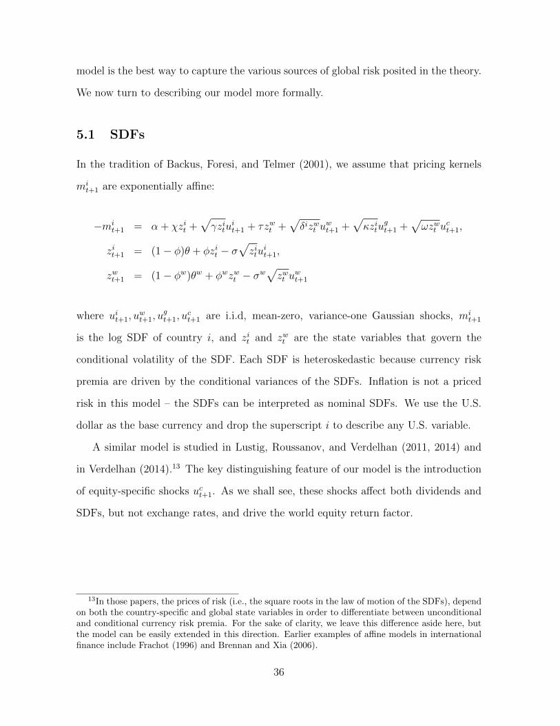
model is the best way to capture the various sources of global risk posited in the theory.

We now turn to describing our model more formally.

5.1 SDFs

In the tradition of Backus, Foresi, and Telmer (2001), we assume that pricing kernels

mit+1 are exponentially affine:

−mit+1 = α + χzit +

√γzitu

it+1 + τzwt +

√δizwt u

wt+1 +

√κzitu

gt+1 +

√ωzwt u

ct+1,

zit+1 = (1− φ)θ + φzit − σ√zitu

it+1,

zwt+1 = (1− φw)θw + φwzwt − σw√zwt u

wt+1

where uit+1, uwt+1, u

gt+1, u

ct+1 are i.i.d, mean-zero, variance-one Gaussian shocks, mi

t+1

is the log SDF of country i, and zit and zwt are the state variables that govern the

conditional volatility of the SDF. Each SDF is heteroskedastic because currency risk

premia are driven by the conditional variances of the SDFs. Inflation is not a priced

risk in this model – the SDFs can be interpreted as nominal SDFs. We use the U.S.

dollar as the base currency and drop the superscript i to describe any U.S. variable.

A similar model is studied in Lustig, Roussanov, and Verdelhan (2011, 2014) and

in Verdelhan (2014).13 The key distinguishing feature of our model is the introduction

of equity-specific shocks uct+1. As we shall see, these shocks affect both dividends and

SDFs, but not exchange rates, and drive the world equity return factor.

13In those papers, the prices of risk (i.e., the square roots in the law of motion of the SDFs), dependon both the country-specific and global state variables in order to differentiate between unconditionaland conditional currency risk premia. For the sake of clarity, we leave this difference aside here, butthe model can be easily extended in this direction. Earlier examples of affine models in internationalfinance include Frachot (1996) and Brennan and Xia (2006).

36

The SDFs depend on country-specific shocks, uit+1, and three global shocks, uwt+1,

ugt+1, and uct+1. We refer to the volatilities of the SDF related to these three shocks

(namely,√δizwt ,

√κzit, and

√ωzwt ) as the market prices of risk of these shocks.

The first shock uwt+1 is priced similarly in each country up to a scaling factor, denoted

δi. Examples of such a shock might be a global financial crisis which affects prices in

all countries in a perfectly correlated fashion, but with differential intensity. To be

parsimonious, we model differences in exposure δi as the only source of heterogeneity

in countries’ SDFs, and fix all the other parameters of the SDFs to be the same across

countries. Countries also differ in their aggregate dividend growth rates.

The model thus features two sources of heterogeneity: one in the SDF and one in

the dividend growth rates. The first source of heterogeneity is necessary to account for

the cross-section of interest rates and currency excess returns. As Lustig, Roussanov,

and Verdelhan (2011) show, high interest rate countries must be characterized by low

exposure (δi) to world shocks for the high interest rate currency to depreciate in bad

times — the key mechanism of any risk-based explanation of carry trade profits. This

first source of heterogeneity entails differences in global equity betas, but if it were

not for the differences in dividend growth rates, the equity betas would line up with

the carry betas. In the data, they do not, consistent with our modeling choice of two

sources of cross-country differences.

The second shock ugt+1 is priced differently across countries, even if countries share

the same exposure κ. An example of this might be a productivity shock that affects

some economies more than others. Finally, as described earlier, the third shock uct+1 is

priced in exactly the same way in all countries.

37

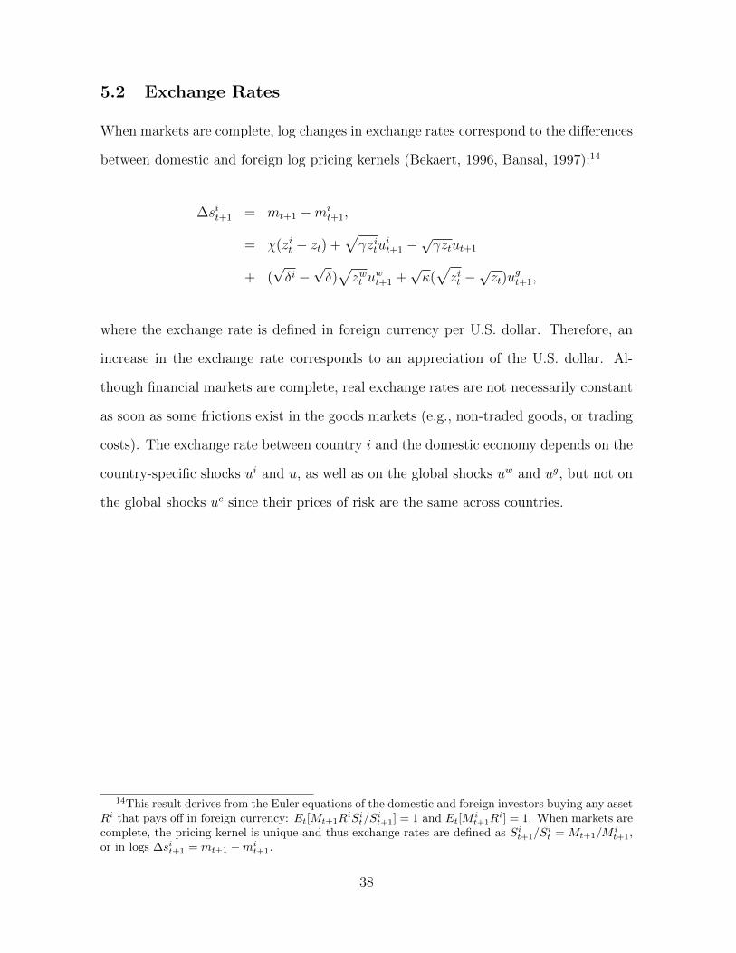
5.2 Exchange Rates

When markets are complete, log changes in exchange rates correspond to the differences

between domestic and foreign log pricing kernels (Bekaert, 1996, Bansal, 1997):14

∆sit+1 = mt+1 −mit+1,

= χ(zit − zt) +√γzitu

it+1 −

√γztut+1

+ (√δi −√δ)√zwt u

wt+1 +

√κ(√zit −

√zt)u

gt+1,

where the exchange rate is defined in foreign currency per U.S. dollar. Therefore, an

increase in the exchange rate corresponds to an appreciation of the U.S. dollar. Al-

though financial markets are complete, real exchange rates are not necessarily constant

as soon as some frictions exist in the goods markets (e.g., non-traded goods, or trading

costs). The exchange rate between country i and the domestic economy depends on the

country-specific shocks ui and u, as well as on the global shocks uw and ug, but not on

the global shocks uc since their prices of risk are the same across countries.

14This result derives from the Euler equations of the domestic and foreign investors buying any assetRi that pays off in foreign currency: Et[Mt+1R

iSit/S

it+1] = 1 and Et[M

it+1R

i] = 1. When markets arecomplete, the pricing kernel is unique and thus exchange rates are defined as Si

t+1/Sit = Mt+1/M

it+1,

or in logs ∆sit+1 = mt+1 −mit+1.

38

5.3 Equity Returns

In order to define equity returns, the model posits a dividend growth process in each

country i:

∆dit+1 = µD + ψzit + ψwzwt + σD

√zitu

it+1 + σwD

√zwt u

wt+1 + σgD

√zitu

gt+1 + σc,iD

√zwt u

ct+1,

where the innovations are the same as those described above. Dividend growth rates re-

spond to both country-specific and global shocks. The only systematic difference across

countries comes from the impact of global shocks uct+1 on dividend growth, governed by

the parameters σc,iD . This source of heterogeneity drives the differences in global equity

market betas.

Innovations to the log gross equity excess return are then:15

re,it+1 − Et(re,it+1) = (σD − k1B

ipdσ)

√zitu

it+1

+ (σwD − k1Cipdσ

w)√zwt u

wt+1 + σgD

√zitu

gt+1 + σc,iD

√zwt u

ct+1,

15In this model, the log price-dividend ratio is affine in the state variables, zit and zwt :

pdit = Aipd +Bi

pdzit + Ci

pdzwt ,

where the constants Aipd, Bi

pd, and Cipd are defined as function of the SDF and dividend growth

parameters. The model is solved in closed form using the standard log-linear approximation for thelog gross return on the aggregate dividend claim:

re,it+1 ≈ k0 + k1pdit+1 − pdit + ∆dit+1,

where k0 and k1 are defined by the Taylor approximation of the log price-dividend ratio pdit aroundits mean. More precisely, the Euler equation applied to the stock market return implies that thecoefficients Ai

pd, Bipd and Ci

pd are defined by:

Aipd = −α+ k0 + k1A

ipd + k1B

ipd(1− φ)θ + k1C

ipd(1− φw)θw + µD,

Bipd = k1B

ipdφ+ ψ − χ+

1

2(√γ + k1B

ipdσ − σD)2 +

1

2(σg

D −√κ)2,

Cipd = k1C

ipdφ

w + ψw − τ +1

2(√δi + k1C

ipdσ

w − σwD)2 +

1

2(√ω − σc,i

D )2.

39

where re,it+1 is the logarithmic gross rate of return on each country’s stock market index

denominated in that country’s currency.

5.4 International CAPM Redux

The equity return of country i expressed in U.S. dollars, denoted re,i,$t+1 , is simply derived

from the equity return of country i in local currency and the change in the exchange

rate:

re,i,$t+1 − Et(re,i,$t+1

)=√γztut+1 +

(σD − k1B

ipdσ −

√γ)√

zituit+1

+(σwD − k1C

ipdσ

w −√δi +√δ)√

zwt uwt+1 + σc,iD

√zwt u

ct+1

+(

(σgD −√κ)√zit +√κzt

)ugt+1.

The foreign equity return expressed in U.S. dollars therefore depends on the foreign

and U.S. specific shocks (ui and u), as well as the global shock captured by the carry

and dollar factors (uw) and (ug) and the world equity shock (uc).

The expected equity excess return from the perspective of a U.S. investor is:

Etre,i,$t+1 − rf,t +

1

2V art

[re,i,$t+1

]= −Covt

[mt+1, r

e,i,$t+1

]= γzt +

(σwD − k1C

ipdσ

w −√δi +√δ)√

δzwt + σc,iD√ωzwt

−(

(σgD −√κ)√zit +√κzt

)√κzt (6)

Note that our assumption of complete markets implies that we only need to verify the

Euler condition for one country’s investor. As soon as the Euler equation is satisfied for

the U.S. investor, for example, it implies that the Euler condition for any foreign investor

is also satisfied. To see this point, recall that the Euler condition for the U.S. investor is

Et[Mt+1R

it+1S

it/S

it+1

]= 1, which implies Et

[M i

t+1Rit+1

]= 1 — the Euler condition of

the representative investor in country i— as well as Et[M j

t+1Rit+1(Sit/S

it+1)(Sjt+1/S

jt )]

=

40

1, the Euler condition of the representative investor in country j.

In order to better understand our empirical approach, next, we express various

factors in the language of the model, namely, the world equity return in U.S. dollars

WMKTt+1, the world equity return in local currencies LWMKTt+1, and the carry and

dollar factors.

5.5 Equity Factors

The innovations to the average world equity market return in local currency terms,

which we define for ease of exposition as the simple average of local equity returns, are:

LWMKTt+1 = re,it+1−Et(re,it+1) = (σwD−k1Ci

pdσw)√zwt u

wt+1 +σgD

√zitu

gt+1 +σc,iD

√zwt u

ct+1,

where x denotes the cross-country average of a variable x.

Country-specific shocks average out, and the world equity market return is only

driven by the global shocks uwt+1, ugt+1, and uct+1. If the law of large numbers applies,

the cross-sectional mean of zit is constant (and equal to θ). The world equity return in

U.S. dollars is:

WMKTt+1 = re,i,$t+1 − Et(re,i,$t+1

)=√γztut+1 +

(σwD − k1Ci

pdσw −√δi +√δ)√

zwt uwt+1

+ σc,iD√zwt u

ct+1 +

((σgD −

√κ)√zit +√κzt

)ugt+1.

5.6 Currency Factors

We first express currency excess returns, which are returns on the following strategy:

the investor borrows at the domestic risk-free rate, converts the amount into foreign

currency and lends at the foreign risk-free rate, converting back the proceeds at the end

of the investment period and paying back the debt. The log currency excess return is

41

thus:16

rxit+1 = rif,t − rf,t −∆sit+1.

The systematic components of currency excess returns are driven by at least two risk

factors (Lustig, Roussanov, and Verdelhan, 2011, 2014, and Verdelhan, 2014), i.e., carry

and dollar factors.

The carry factor is the excess returns of a strategy that invests in high- and borrows

in low-interest rate currencies:

Carryt+1 =1

NH

∑i∈H

rxit+1 −1

NL

∑i∈L

rxit+1,

where NH (NL) denotes the number of high (low) interest rate currencies in the sample.

For the sake of exposition, assume that most of the cross-country difference in inter-

est rates is due to their exposure (δi) to the world state variable. In this case, baskets

of high and low interest rate currencies will exhibit the same level of country-specific

16The risk-free rate in country i, denoted rif,t, is given by:

rif,t = −Et [mit+1]− 1

2V art[m

it+1] = α+

(χ− 1

2(γ + κ)

)zit +

(τ − 1

2(δi + ω)

)zwt .

The interest rate difference, or forward discount, between country i and the U.S is therefore equal to:

rif,t − rf,t =

(χ− 1

2(γ + κ)

)(zit − zt)−

1

2

(δi − δ

)zwt .

The expected currency excess return is therefore:

Et

(rxit+1

)= rif,t − rf,t − Et

(∆sit+1

)=

1

2V art(mt+1)− 1

2V art(m

it+1)

=1

2(γ + κ)(zt − zit) +

1

2(δ − δi)zwt .

If the SDFs were not hetereoscedastic, the expected currency excess returns would be constant and theuncovered interest rate parity, which is strongly rejected in the data, would be satisfied in the model.

42

volatility, assuming that the law of large numbers holds.17 Under this assumption,

innovations to the carry factor only depend on shocks uw, not on shocks ug.

Carryt+1 − Et (Carryt+1) =

(√δiL

−√δiH)√

zwt uwt+1,

where xiH

and xiL

denote the cross-sectional average of the variable x across countries

in the high- and low-interest rate portfolios: xiH

= 1NH

∑i∈H x

i, xiL

= 1NL

∑i∈L x

i.

The dollar risk factor is the average of all currency excess returns defined in U.S.

dollars:

Dollart+1 =1

N

∑i

rxit+1,

where N denotes the number of currencies in the sample. In large baskets of currencies,

foreign country-specific shocks average out (again assuming that there are enough cur-

rencies in the baskets for the law of large numbers to apply). As a result, innovations

to the dollar risk factor depend on both U.S.-specific and world shocks, but not on

country-specific shocks:

Dollart+1 − Et (Dollart+1) =√γztut+1

+(√

δ −√δi)√

zwt uwt+1 +

√κ(√

zt −√zit

)ugt+1.

If the U.S. SDF exhibits the average exposure to shocks uw (i.e., δi = δ), the

dollar factor is orthogonal to the carry factor. Under that assumption, the dollar factor

captures shocks ug, while the carry factor captures shocks uw.

17In practice of course, the number of currencies is small (the dataset used in this paper containsat most 39 currencies). As a result, the law of large numbers is only an approximation used here toprovide intuition.

43

5.7 Connecting the Model to the Empirics

The world equity return, LWMKTt+1, built from returns in local currencies, does

not span all systematic shocks: it depends on shocks uw, ug, and uc, but not on the

U.S. shocks u. These shocks u are systematic from the perspective of the U.S. investor,

although not from the perspective of other investors. They appear in the cross-section of

equity excess returns because the returns need to be expressed in one common currency

(e.g., the U.S. dollar).

In contrast, the world equity return in U.S. dollars WMKTt+1 contains all the

systematic shocks that drive foreign equity returns. At first sight, it appears as a

sufficient tool to measure aggregate risk, without the need to add any bilateral exchange

rates. This result contrasts with the findings of Adler and Dumas (1983) because the

exchange rate is endogenous in our setup. In practice, however, even in this simple

model, the world equity return in U.S. dollars is an imperfect measure of risk in the

(obviously general) case when the econometrician does not know the country-specific

and global state variables.

To see this point, consider the time-variation in the quantity and market price of

aggregate risk, starting with the betas. The betas on the global shocks uw and uc are

constant, while the betas on the global shocks ug are not. The total beta on the world

equity return in U.S. dollars WMKTt+1 is time-varying, following the dynamics of the

country-specific state variables z and zi:

βiWMKT,t = 1 +σwD − k1C

ipdσ

w −√δi +√δ

σwD − k1Cipdσ

w −√δi +√δ

+σc,iD

σc,iD

+(σgD −

√κ)√zit +√κzt

(σgD −√κ)√zit +√κzt

(7)

In our simple setup, all country-specific state variables zi are characterized by the

same persistence and volatility. However, in actual data, country-specific state variables

seem very likely to evolve at different frequencies, confounding estimation.

Market prices of risk are also time-varying in our simple model. Expected excess

44

returns are the product of betas and market prices of risk, i.e., the market price of

world equity risk is the ratio of the expected excess return, defined in Equation (6), to

the beta in Equation (7). The price of risk thus also varies with the country-specific

and global state variables (z, zi, and zw). If those state variables were known to the

econometrician, a conditional asset pricing experiment could recover the time-variation

in the quantities and prices of risk. In practice however, the state variables are not

known, forcing reliance on rolling windows or other such empirical approaches.

The issue becomes even more acute if the heteroskedasticity of the uw or uc shocks

were to depend on both global and country-specific state variables.18 In that case, the

aggregate market beta βiWMKT,t also depends on the global state variable zw. The criti-

cal issue here is that if the local and global state variables evolve at different frequencies,

it becomes impossible to use a single beta to perfectly summarize the time-variation in

two state variables.

Taken together, the world equity return expressed in U.S. dollars bundles variables

with different time-dynamics together. This makes it difficult to use this single factor

to uncover risk exposures in international asset pricing. While our simple model with

endogenous exchange rates suggests that we should go back to the World CAPM, the

heteroskedasticity of the SDF implies that this single-factor model would struggle to

accurately capture the risk-return tradeoff in practice.

This motivates our choice of a multiple-factor model. With LWMKT , Carry, and

Dollar, we can summarize all the shocks in the system, and we can allow all quantities

18Lustig, Roussanov, and Verdelhan (2011, 2014) and Verdelhan (2014) consider this variation inorder to reproduce some features of the currency markets. In the context of our model, the law ofmotion of the log SDF would be:

−mit+1 = α+ χzit +

√γzitu

it+1 + τzwt +

√δizwt + λzitu

wt+1 +

√κzitu

gt+1 +

√ωzwt u

ct+1

We do not consider that variation here as it does not admit a closed-form solution for equity returnsand betas.

45

and prices of risk to have their own time-dynamics. When we empirically implement

the model in the data, the only difference lies in the approach to aggregation, i.e., we

weight countries and currencies by stock market capitalizations, instead of the equal

weights that we employ in the model for ease of exposition.

The model has three additional implications that we check in the data. First, the

carry and dollar factors should matter even for equity excess returns expressed in local

currency. Likewise, the equity factor LWMKTt+1, built without introducing exchange

rates, should be correlated with the carry and dollar factors. Second, despite exchange

rates being endogenous, exchange rate shocks in this model do not span equity returns.

Shocks uc affect equity returns but do not affect exchange rates, because their impact

is exactly the same across countries. Equity and currency markets therefore appear

segmented to an extent. Third, while using bilateral exchange rates as risk factors

directly is consistent with the model, they are also driven by country-specific shocks

that are irrelevant to asset pricing and thus weaken the identification of aggregate risk.

5.8 Shortcomings of the Model

The model is parsimonious and can be solved in closed form. But its simplicity entails

some shortcomings when compared to the data. The main weakness of the model lies

in its implied betas.

In the data, global equity and currency betas are clearly time-varying. Moreover, the

global equity, carry, and dollar betas are not highly correlated. The time-series correla-

tions (obtained country-by-country) range from −0.7 to 0.7 for the LWMKT −Dollar,

LWMKT −Carry, and Dollar−Carry pairs. Across countries, these correlations are

close to zero. Our asset pricing estimates allow for these factor-specific dynamics in the

quantities of risk.

But in the model, betas are either constant or too smooth. A univariate regression

46

of equity excess returns in U.S. dollars on the carry factor, for example, delivers a

constant beta; the data suggest otherwise. Time-variation in all betas can be obtained

in the model by assuming that the market prices of risk (i.e., the square roots in the

SDFs) depend not only on one but on two state variables. In this case, however, the

model does not admit a closed-form. For the sake of clarity, we choose to focus on a

model that delivers all objects of interest in closed-form.

5.9 Simulating the Model

We simulate the model in order to better understand the drivers of our empirical results.

We begin by calibrating key parameters of the model, and present these calibration

parameters in Table 3.

The boundaries of the parameter δ (i.e., δl and δh) are determined to match the mean

interest-rate differential of the Japanese yen and the Australian dollar against the U.S.

dollar over the period January 1976 to April 2013 (-3.18 % and 3.27 %, respectively).

All parameters governing the state variable dynamics and the parameters τ , χ and

γ governing the stochastic discount factor are from Lustig, Roussanov, and Verdelhan

(2014).

The parameter α is calibrated to match an average annualized nominal risk-free rate

of 4.5% given the parameter values for χ, γ, κ, τ , ω and the average δ.

The remaining parameters are set to match the empirical pairwise correlations be-

tween the equity and currency factors (reported in the Online Appendix).

The model delivers reasonable interest rates, exchange rates, equity, and currency

excess returns as can be seen in Table 4 below.

Figure 9 shows what happens when we estimate our empirical specifications on these

simulated data from the model – it is the counterpart to Figure 5, but estimated using

simulated data from the model. The vertical axis corresponds to average excess returns

47

Table 3Parameter Values

This table reports the parameter values used to simulate the model. The boundaries of the parameterδ (i.e., δl and δh) are determined to match the mean interest-rate differential of the Japanese yen andthe Australian dollar against the U.S. dollar over the period January 1976 to April 2013 (-3.18 % and3.27 %, respectively). All parameters governing the state variable dynamics and the parameters τ ,χ and γ governing the stochastic discount factor are from Lustig, Roussanov and Verdelhan (2014).The parameter α is calibrated to match an average annualized nominal risk-free rate of 4.5% giventhe parameter values for χ, γ, κ, τ , ω and the average δ. The remaining parameters are set to matchthe empirical pairwise correlations between the equity and currency factors. The law of motion of thestochastic discount factor (Panel A), the state variable dynamics (Panel B) and the dividend growthprocess (Panel C) are reported at the top of each panel.

Panel A: Stochastic discount factor

−mit+1 = α+ χzit +

√γzitu

it+1 + τzwt +

√δizwt u

wt+1 +

√κzitu

gt+1 +

√ωzwt u

ct+1

SDF Heterogeneity

α (%) χ γ κ τ ω δHC δL δH

4.5 0.89 0.04 2.2 0.06 2.2 0.36 0.10 0.61

Panel B: State variable dynamics

zit+1 = (1− φ)θ + φzit − σ√zitu

it+1 zwt+1 = (1− φw)θw + φwzwt − σw

√zwt u

wt+1

φ θ (%) σ (%) φw θw (%) σw (%)

0.91 0.77 0.68 0.99 2.09 0.28

Panel C: Dividend growth rate

∆dit+1 = µD + ψzit + ψwzwt + σD

√zitu

it+1 + σgD

√zitu

gt+1 + σwD

√zwt u

wt+1 + σc,iD

√zwt u

ct+1

Dividends Heterogeneity

µD (%) ψ ψw σD σgD σwD σcD σc,LD σc,HD

2.71 0 -1.1 0.12 0.05 0.01 0.19 0.16 0.23

48

Table 4Descriptive Statistics of Simulated Equity and Foreign Exchange Series

This table compares cross-sectional moments of simulated equity and foreign exchange series (PanelA) with their empirical counterparts (Panel B). Moments are defined as the cross-sectional meanand standard deviation of the time-series mean, standard deviation, and first-order autocorrelation(AC1) of the following variables: country equity returns denominated in either local currency (rei)or U.S. Dollars (re$), the price-dividend ratio in log-form (p − d), the dividend growth rate (∆d),the country risk-free rates (rif ), the log changes in bilateral exchange rates (∆s) and the interest ratedifferences between a foreign and the domestic currency (i∗ − i). The last column reports time-seriesmoments for the United States. The model is calibrated using parameter values reported in Table 3.It is simulated for a population of 45 countries and one million periods. Empirical moments refer todeveloped countries. Except for the price-dividend ratio, means and standard deviations are annualizedand reported in percentage terms.

Moments A: Simulation B: Data

Mean Std Mean Std US

E(rei) 10.39 1.83 10.05 2.43 10.29σ(rei) 9.93 0.84 20.38 3.73 15.23AC1(rei) 0.02 0.00 0.11 0.06 0.06

E(re$) 10.36 1.83 10.34 1.75 10.29σ(re$) 14.88 2.37 22.84 3.83 15.23AC1(re$) 0.00 0.00 0.07 0.05 0.06

E(p− d) 5.46 0.37 3.53 0.36 3.60σ(p− d) 0.03 0.01 0.40 0.11 0.47AC1(p− d) 0.99 0.01 0.98 0.01 0.99

E(∆d) 4.95 0.01 7.65 2.60 6.02σ(∆d) 9.96 0.81 14.79 5.18 7.18AC1(∆d) 0.02 0.00 0.20 0.17 0.46

E(rif ) 4.50 1.93 5.10 2.17 5.03σ(rif ) 1.64 0.10 1.33 0.50 0.97AC1(rif ) 0.99 0.00 0.84 0.15 0.97

σ(∆s) 12.48 1.82 10.15 2.91 -AC1(∆s) -0.01 0.00 0.00 0.09 -

E(i∗ − i) 0.00 1.93 0.93 2.82 -σ(i∗ − i) 0.19 0.04 1.03 0.37 -AC1(i∗ − i) 0.93 0.01 0.73 0.24 -

49

from simulated data. The horizontal axis corresponds to predicted excess returns from

the World CAPM, the International CAPM, and our three-factor model all estimated

using the simulated data, using rolling-windows in order to capture time-variation in

quantities and prices of risk. The figure presents a striking demonstration of the dif-

ference: the World CAPM and the International CAPM both fit the simulated data

rather poorly, while our model accurately describes the cross-section of returns.

Our next step is to attempt to use our model framework to explore the portfolio

choice and hedging strategy of global investors.

6 Optimal Currency Hedging

Black (1989) derives a striking result: the optimal amount of currency hedging is the

same for every investor in the world. It depends on only three variables: the average

world market portfolio expected excess return (µm), the average world market portfolio

excess return variance (σ2m), and the average exchange rate variance (σ2

e).

Black (1989) shows that the fraction of exchange risk hedged should be equal to:

µm − σ2m

µm − 12σ2e

.

This striking result continues to serve as something of a benchmark to this day. But it

is derived in a mean-variance efficient world that does not encompass our model. We

thus revisit the issue in our framework, by solving for the optimal portfolio and then

inspecting the optimal currency portfolio investment strategy of an atomistic interna-

tional investor.

50

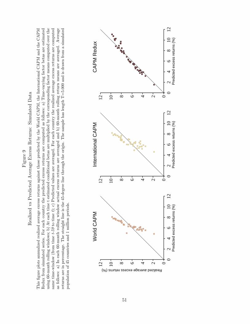
Fig

ure

9R

ealize

dvs

Pre

dic

ted

Ave

rage

Exce

ssR

eturn

s:Sim

ula

ted

Dat

a

Th

isfi

gure

plo

tsan

nu

aliz

edre

aliz

edav

erag

eex

cess

retu

rns

again

stth

ose

pre

dic

ted

by

the

Worl

dC

AP

M,

the

Inte

rnati

on

al

CA

PM

an

dth

eC

AP

MR

edu

xfr

omsi

mu

late

dse

ries

.F

orea

chco

untr

yth

ep

red

icte

dex

cess

retu

rns

are

com

pu

ted

as

foll

ows:

a)

Tim

e-va

ryin

gfa

ctor

bet

as

are

esti

mate

du

sin

g60

-mon

thro

llin

gw

ind

ows;

b)

At

each

tim

et

esti

mate

dco

nd

itio

nal

bet

as

are

mu

ltip

lied

by

the

corr

esp

on

din

gfa

ctor

mea

ns

com

pu

ted

over

the

sam

eti

me-

win

dow

(fro

mti

met-59

toti

met)

;c)

Pre

dic

ted

valu

esare

aver

aged

.F

or

each

cou

ntr

yth

ere

ali

zed

aver

age

exce

ssre

turn

sare

com

pu

ted

asfo

llow

s:a)

Inea

ch60

-mon

thro

llin

gw

ind

owact

ual

exce

ssre

turn

sare

aver

aged

an

db

)60-m

onth

roll

ing

retu

rnm

ean

sare

aver

aged

.A

vera

ge

retu

rns

are

inp

erce

nta

ge.

Th

est

raig

ht

lin

eis

the

45-d

egre

eli

ne

thro

ugh

the

ori

gin

.T

he

sam

ple

has

len

gth

T=

5.0

00

an

dis

dra

wn

from

asi

mu

late

dp

opu

lati

onof

45co

untr

ies

and

1m

illi

onp

erio

ds.

02

46

810

12024681012

W

orld

CA

PM

Realized average excess returns (%)

Pre

dict

ed e

xces

s re

turn

s (%

)0

24

68

1012

024681012In

tern

atio

nal C

AP

M

Pre

dict

ed e

xces

s re

turn

s (%

)0

24

68

1012

024681012

C

AP

M R

edux

Pre

dict

ed e

xces

s re

turn

s (%

)

51

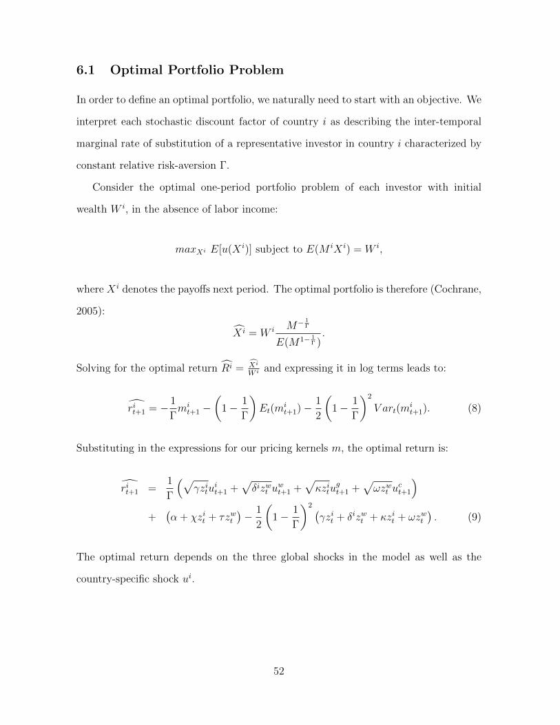
6.1 Optimal Portfolio Problem

In order to define an optimal portfolio, we naturally need to start with an objective. We

interpret each stochastic discount factor of country i as describing the inter-temporal

marginal rate of substitution of a representative investor in country i characterized by

constant relative risk-aversion Γ.

Consider the optimal one-period portfolio problem of each investor with initial

wealth W i, in the absence of labor income:

maxXi E[u(X i)] subject to E(M iX i) = W i,

where X i denotes the payoffs next period. The optimal portfolio is therefore (Cochrane,

2005):

X i = W i M− 1Γ

E(M1− 1Γ ).

Solving for the optimal return Ri = Xi

W i and expressing it in log terms leads to:

rit+1 = − 1

Γmit+1 −

(1− 1

Γ

)Et(m

it+1)− 1

2

(1− 1

Γ

)2

V art(mit+1). (8)

Substituting in the expressions for our pricing kernels m, the optimal return is:

rit+1 =1

Γ

(√γzitu

it+1 +

√δizwt u

wt+1 +

√κzitu

gt+1 +

√ωzwt u

ct+1

)+

(α + χzit + τzwt

)− 1

2

(1− 1

Γ

)2 (γzit + δizwt + κzit + ωzwt

). (9)

The optimal return depends on the three global shocks in the model as well as the

country-specific shock ui.

52

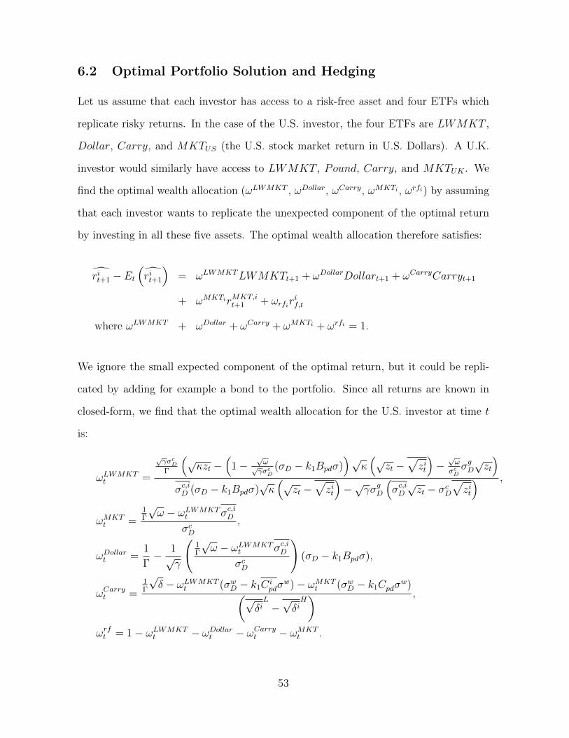
6.2 Optimal Portfolio Solution and Hedging

Let us assume that each investor has access to a risk-free asset and four ETFs which

replicate risky returns. In the case of the U.S. investor, the four ETFs are LWMKT ,

Dollar, Carry, and MKTUS (the U.S. stock market return in U.S. Dollars). A U.K.

investor would similarly have access to LWMKT , Pound, Carry, and MKTUK . We

find the optimal wealth allocation (ωLWMKT , ωDollar, ωCarry, ωMKTi , ωrfi) by assuming

that each investor wants to replicate the unexpected component of the optimal return

by investing in all these five assets. The optimal wealth allocation therefore satisfies:

rit+1 − Et(rit+1

)= ωLWMKTLWMKTt+1 + ωDollarDollart+1 + ωCarryCarryt+1

+ ωMKTirMKT,it+1 + ωrfir

if,t

where ωLWMKT + ωDollar + ωCarry + ωMKTi + ωrfi = 1.

We ignore the small expected component of the optimal return, but it could be repli-

cated by adding for example a bond to the portfolio. Since all returns are known in

closed-form, we find that the optimal wealth allocation for the U.S. investor at time t

is:

ωLWMKTt =

√γσc

D

Γ

(√κzt −

(1−

√ω√γσc

D(σD − k1Bpdσ)

)√κ(√

zt −√zit

)−√ω

σcDσgD√zt

)σc,iD (σD − k1Bpdσ)

√κ(√

zt −√zit

)−√γσgD

(σc,iD√zt − σcD

√zit

) ,

ωMKTt =

1Γ

√ω − ωLWMKT

t σc,iDσcD

,

ωDollart =1

Γ− 1√γ

(1Γ

√ω − ωLWMKT

t σc,iDσcD

)(σD − k1Bpdσ),

ωCarryt =1Γ

√δ − ωLWMKT

t (σwD − k1Cipdσ

w)− ωMKTt (σwD − k1Cpdσ

w)(√δiL

−√δiH) ,

ωrft = 1− ωLWMKTt − ωDollart − ωCarryt − ωMKT

t .

53

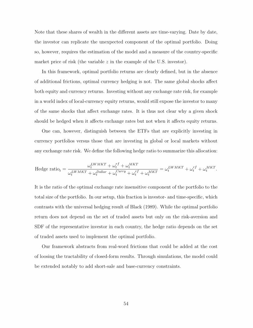
Note that these shares of wealth in the different assets are time-varying. Date by date,

the investor can replicate the unexpected component of the optimal portfolio. Doing

so, however, requires the estimation of the model and a measure of the country-specific

market price of risk (the variable z in the example of the U.S. investor).

In this framework, optimal portfolio returns are clearly defined, but in the absence

of additional frictions, optimal currency hedging is not. The same global shocks affect

both equity and currency returns. Investing without any exchange rate risk, for example

in a world index of local-currency equity returns, would still expose the investor to many

of the same shocks that affect exchange rates. It is thus not clear why a given shock

should be hedged when it affects exchange rates but not when it affects equity returns.

One can, however, distinguish between the ETFs that are explicitly investing in

currency portfolios versus those that are investing in global or local markets without

any exchange rate risk. We define the following hedge ratio to summarize this allocation:

Hedge ratiot =ωLWMKTt + ωrft + ωMKT

t

ωLWMKTt + ωDollart + ωCarryt + ωrft + ωMKT

t

= ωLWMKTt + ωrft + ωMKT

t .

It is the ratio of the optimal exchange rate insensitive component of the portfolio to the

total size of the portfolio. In our setup, this fraction is investor- and time-specific, which

contrasts with the universal hedging result of Black (1989). While the optimal portfolio

return does not depend on the set of traded assets but only on the risk-aversion and

SDF of the representative investor in each country, the hedge ratio depends on the set

of traded assets used to implement the optimal portfolio.

Our framework abstracts from real-word frictions that could be added at the cost

of loosing the tractability of closed-form results. Through simulations, the model could

be extended notably to add short-sale and base-currency constraints.

54

7 Conclusion

In this paper, we show that currency risk is priced in international equity portfolios.

We do so using a new set of three factors, namely, a global equity factor denominated in

local currencies, and two currency factors, dollar and carry, which are constructed from

the space of global currency excess returns. Our results on the pricing of currency risk

using this model are obtained from a comprehensive set of equities from 46 developed

and emerging countries spanning value, growth, and country index returns from 1976

to the present. We also find that our model outperforms the World and International

CAPM, as well as the Fama-French three and four factor models in our sample, and find

evidence of substantial exposure to currency risk in the universe of global mutual funds

and hedge funds, suggesting that whether exposure to international markets is direct

or indirect, currency risk is a significant factor affecting the returns of international

investors.

We set up a simple complete-markets model of international equities with endoge-

nous exchange rates, and show that this model is well able to replicate our key empirical

findings. The model also enables us to derive the optimal asset portfolio weights for an

atomistic international investor. In our framework, the optimal investment in currency

assets for such an investor varies over time and across investor locations, contrary to

the famous result of Black (1989) who operates in a simpler mean-variance preference

setting.

References

Adler, Michael and Bernard Dumas, “International Portfolio Choice and Corpo-

ration Finance: A Synthesis,” The Journal of Finance, 1983, 38 (3), 925–984.

55

Andrews, Donald W.K., “Heteroskedasticity and Autocorrelation Consistent Co-

variance Matrix Estimation,” Econometrica, 1991, 59 (1), 817–858.

Asness, Clifford S., Tobias J. Moskowitz, and Lasse Heje Pedersen, “Value

and Momentum Everywhere,” The Journal of Finance, 2013, 68 (3), 929–985.

Backus, David, Silverio Foresi, and Chris Telmer, “Affine Term Structure Models

and the Forward Premium Anomaly,” Journal of Finance, 2001, 56 (1), 279–304.

Bansal, Ravi, “An Exploration of the Forward Premium Puzzle in Currency Markets,”

Review of Financial Studies, 1997, 10, 369–403.

Banz, Rolf W., “The Relationship Between Return and Market Value of Common

Stocks,” Journal of Financial Economics, 1981, 9 (1), 3–18.

Bekaert, Geert, “The Time Variation of Expected Returns and Volatility in Foreign-

Exchange Markets,” Journal of Business and Economic Statistics, 1995, 13 (4),

397–408.

, “The Time Variation of Risk and Return in Foreign Exchange Markets: A General

Equilibrium Perspective,” The Review of Financial Studies, 1996, 9 (2), 427–470.

and Campbell R. Harvey, “Time-Varying World Market Integration,” The

Journal of Finance, 1995, 50 (2), 403–444.

and , “Foreign Speculators and Emerging Equity Markets,” Journal of Fi-

nance, 2000, 55 (2), 565 – 613.

and , “Emerging Equity Markets in a Globalizing World,” Working Paper

Duke University, 2014.

56

and Robert J. Hodrick, “Characterizing Predictable Components in Excess

Returns on Equity and Foreign Exchange Markets,” The Journal of Finance, 1992,

47, 467–509.

and Xiaozheng Sandra Wang, “Globalization and Asset Prices,” Working

Paper Columbia University, 2009.

, Campbell R. Harvey, and Christian Lundblad, “Equity Market Liberal-

ization in Emerging Markets,” Journal of Financial Research, 2003, 26, 275–299.

, , and , “Liquidity and Expected Returns: Lessons from Emerging

Markets,” Review of Financial Studies, 2007, 20 (6), 1783–1831.

, , , and Stephan Siegel, “Global Growth Opportunities and Market

Integration,” The Journal of Finance, 2007, 62 (3), 1081–1137.

, , Christian T. Lundblad, and Stephan Siegel, “What Segments Equity

Markets?,” Review of Financial Studies, 2011, 24 (12), 3847–3890.

, Robert J. Hodrick, and Xiaoyan Zhang, “International Stock Return Co-

movements,” Journal of Finance, 2009, 64, 2591–2626.

Brennan, Michael J and Yihong Xia, “International Capital Markets and Foreign

Exchange Risk,” Review of Financial Studies, 2006, 19 (3), 753–795.

Bryzgalova, Svetlana, “Spurious Factors In Linear Asset Pricing Models,” 2015.

Working Paper.

Campbell, John Y., Karine Serfaty De Medeiros, and Luis M. Viceira,

“Global Currency Hedging,” The Journal of Finance, 2010, 65 (1), 87–121.

Carhart, Mark M., “On Persistence in Mutual Fund Performance,” The Journal of

Finance, 1997, 52 (1), 57–82.

57

Chaieb, Ines and Vihang Errunza, “International Asset Pricing Under Segmenta-

tion and PPP Deviations,” Journal of Financial Economics, November 2007, 86

(2), 543–578.

Chan, Kakeung C., Andrew G. Karolyi, and Rene M. Stulz, “Global Financial

Markets and the Risk Premium on U.S. Equity,” Journal of Financial Economics,

October 1992, 32 (2), 137–167.

Chan, Louis KC, Yasushi Hamao, and Josef Lakonishok, “Fundamentals and

Stock Returns in Japan.,” The Journal of Finance, 1991, 46 (5), 1739–1764.

Chinn, Menzie D and Hiro Ito, “A New Measure of Financial Openness,” Journal

of Comparative Policy Analysis, 2008, 10 (3), 309–322.

Chui, Andy C.W., Sheridan Titman, and K.C. John Wei, “Individualism and

Momentum Around the World,” The Journal of Finance, 2010, 65 (1), 361–392.

Cochrane, John H., Asset Pricing, Princeton University Press, Princeton, 2005.

Daniel, Kent and Sheridan Titman, “Evidence on the Characteristics of Cross

Sectional Variation in Stock Returns,” The Journal of Finance, 1997, 52 (1), 1–33.

De Santis, Giorgio and Bruno Gerard, “How Big is the Premium for Currency

Risk ?,” Journal of Financial Economics, 1998, 49, 375–412.

Dumas, Bernard and Bruno Solnik, “The World Price of Foreign Exchange Risk,”

Journal of Finance, 1995, 50 (2), 445–479.

Evans, Martin DD and Richard K Lyons, “Order Flow and Exchange Rate Dy-

namics,” The Journal of Political Economy, 2002, 110 (1), 170–180.

Fama, Eugene F. and James D. MacBeth, “Risk, Return, and Equilibrium: Em-

pirical Tests,” The Journal of Political Economy, 1973, 81 (3), 607–636.

58

and Kenneth R. French, “Common Risk Factors in the Returns on Stocks and

Bonds,” Journal of Financial Economics, February 1993, 33 (1), 3–56.

and , “Size, Value, and Momentum in International Stock Returns,” Journal

of Financial Economics, September 2012, 105 (3), 457–472.

Ferson, Wayne E. and Campbell R. Harvey, “The Risk and Predictability of

International Equity Returns,” Review of Financial Studies, 1993, 6 (3), 527–566.

and , “Sources of Risk and Expected Returns in Global Equity Markets,”

Journal of Banking & Finance, September 1994, 18 (4), 775–803.

Frachot, Antoine, “A Reexamination of the Uncovered Interest Rate Parity Hypoth-

esis,” Journal of International Money and Finance, 1996, 15 (3), 419–437.

Froot, Kenneth A. and Kenneth Rogoff, “Perspectives on PPP and Long-Run

Real Exchange Rates,” Handbook of International Economics, 1995, p. 1.

and Tarun Ramadorai, “Currency Returns, Intrinsic Value, and Institutional

Investor Flows,” The Journal of Finance, 2005, 60 (3), 1535–1566.

Gibbons, Michael R., Stephen A. Ross, and Jay Shanken, “A Test of the

Efficiency of a Given Portfolio,” Econometrica, 1989, 57, 1121–1152.

Glen, Jack and Philippe Jorion, “Currency Hedging for International Portfolios,”

The Journal of Finance, 1993, 48 (5), 1865–1886.

Griffin, John M., “International Competition and Exchange Rate Shocks: A Cross-

Country Industry Analysis of Stock Returns,” Review of Financial Studies, March

2001, 14 (1), 215–241.

59

, Xiuqing Ji, and J. Spencer Martin, “Momentum Investing and Business

Cycle Risk: Evidence from Pole to Pole,” The Journal of Finance, 2003, 58 (6),

2515–2547.

Harvey, Campbell R., “The World price of Covariance Risk,” Journal of Finance,

1991.

, Bruno Solnik, and Guofu Zhou, “What Determines Expected International

Asset Returns?,” Annals of Economics and Finance, 2002, 3 (2), 249–98.

Hou, Kewei, Andrew G. Karolyi, and Bong-Chan Kho, “What Factors Drive

Global Stock Returns?,” Review of Financial Studies, May 2011, 24 (8), 2527–2574.

Karolyi, Andrew G. and Rene M. Stulz, “Why Do Markets Move Together? An

Investigation of US-Japan Stock Return Comovements,” The Journal of Finance,

1996, 51 (3), 951–986.

and Ying Wu, “The Role of Investability Restrictions on Size, Value, and Mo-

mentum in International Stock Returns,” Working Paper Cornell University, 2014.

, Kuan-Hui Lee, and Mathijs A. van Dijk, “Understanding Commonality in

Liquidity Around the World,” Journal of Financial Economics, 2012, 105 (1), 82

– 112.

Korajczyk, Robert and Claude Viallet, “An Empirical Investigation of Interna-

tional Asset Pricing,” Review of Financial Studies, 1989, 2 (4), 553–585.

Kroencke, Tim A, Felix Schindler, and Andreas Schrimpf, “International Diver-

sification Benefits with Foreign Exchange Investment Styles*,” Review of Finance,

2013, p. rft047.

60

Lane, Philip R. and Gian Maria Milesi-Ferretti, “The External Wealth of Nations

Mark II: Revised and Extended Estimates of Foreign Assets and Liabilities, 1970–

2004,” Journal of International Economics, 2007, 73, 223–250.

Lettau, Martin, Matteo Maggiori, and Michael Weber, “Conditional Risk Pre-

mia in Currency Markets and Other Asset Classes,” Journal of Financial Eco-

nomics, forthcoming, 2013.

Lewellen, Jonathan and Stefan Nagel, “The Conditional CAPM Does Not Explain

Asset-Pricing Anomalies,” Journal of Financial Economics, November 2006, 82

(2), 289–314.

Lewis, Karen K, “Global Asset Pricing,” Annual Review of Financial Economics,

2011, 3, 435–466.

Lintner, John, “The Valuation of Risk Assets and the Selection of Risky Investments

in Stock Portfolios and Capital Budgets,” The Review of Economics and Statistics,

1965, 47 (1), 13–37.

Lo, Andrew W. and A. Craig MacKinlay, “Data-Snooping Biases in Tests of

Financial Asset Pricing Models,” Review of Financial studies, 1990, 3 (3), 431–

467.

Lustig, Hanno and Adrien Verdelhan, “The Cross-Section of Currency Risk Pre-

mia and US Consumption Growth Risk,” Working Paper, NBER, 2005, 11104.

and , “The Cross-Section of Foreign Currency Risk Premia and Consumption

Growth Risk,” American Economic Review, 2008, 97, 89–117.

and , “Does Market Incompleteness Help to Explain Exchange Rates? A

Quantitative Assessment,” 2015. MIT Sloan Working Paper.

61

, Nikolai Roussanov, and Adrien Verdelhan, “Common Risk Factors in Cur-

rency Markets,” Review of Financial Studies, August 2011, 24 (11), 3731–3777.

, , and , “Countercyclical Currency Risk Premia,” Journal of Financial

Economics, 2014, 111 (3), 527–553.

Maggiori, Matteo, “The U.S. Dollar Safety Premium,” 2012. NYU Working Paper.

Malkhozov, Aytek, Philippe Mueller, Andrea Vedolin, and Gyuri Venter,

“Funding Liquidity CAPM: International Evidence,” Working Paper, 2014.

Meese, Richard A. and Kenneth Rogoff, “Empirical Exchange Rate Models Of

The Seventies: Do They Fit Out Of Sample?,” Journal of International Economics,

1983, 14 (1), 3–24.

Menkhoff, Lukas, Lucio Sarno, Maik Schmeling, and Andreas Schrimpf,

“Carry Trades and Global Foreign Exchange Rate Volatility,” Journal of Finance,

2012, 67 (2), 681–718.

Newey, Whitney K. and Kenneth D. West, “A Simple, Positive Semi-Definite,

Heteroskedasticity and Autocorrelation Consistent Covariance Matrix,” Economet-

rica, 1987, 55 (3), 703–708.

Patton, Andrew J, Tarun Ramadorai, and Michael Streatfield, “Change You

Can Believe In? Hedge Fund Data Revisions,” Journal of Finance, Forthcoming,

2013.

Ramadorai, Tarun, “Capacity Constraints, Investor Information, and Hedge Fund

Returns,” Journal of Financial Economics, 2013, 107, 401–416.

Roll, Richard, “A Critique of the Asset Pricing Theory’s Tests Part I: On Past and

Potential Testability of the Theory,” Journal of Financial Economics, 1977, 4 (2),

129–176.

62

Ross, Stephen, “The Arbitrage Theory of Capital Asset Pricing,” Journal of Eco-

nomic Theory, 1976, 13 (3), 341–360.

Sercu, Piet, “A Generalisation of the International Asset Pricing Model,” Revue de

l’Association Francaise de Finance, 1980, 1 (1), 91–135.

Shanken, Jay, “On the Estimation of Beta-Pricing Models,” Review of Financial

Studies, 1992, 5 (1), 1–55.

Sharpe, William F, “Capital Asset Prices: A Theory of Market Equilibrium under

Conditions of Risk*,” The Journal of Finance, 1964, 19 (3), 425–442.

Solnik, Bruno H, “An Equilibrium Model of the International Capital Market,” Jour-

nal of Economic Theory, 1974, 8, 500–524.

Stehle Richard, “An Empirical Test of the Alternative Hypotheses of National and

International Pricing of Risky Assets,” The Journal of Finance, 1977, 32 (2), 493–

502.

Stehle, Richard, “An Empirical Test of the Alternative Hypotheses of National and

International Pricing of Risky Assets,” The Journal of Finance, 1977, 32 (2), 493–

502.

Stulz, Rene M., “A Model of International Asset Pricing,” Journal of Financial

Economics, 1981, 9, 383–406.

, “International Portfolio Choice and Asset Pricing: An Integrative Survey,” The

Handbook of Modern Finance. North-Holland, Amsterdam, February 1995.

Verdelhan, Adrien, “The Share of Systematic Variation in Bilateral Exchange Rates,”

MIT Sloan Working Paper, 2014.

63

Appendix

A A Brief Review of the Literature on International

Asset Pricing

Early theoretical work in international asset pricing generally assumed that consump-tion and investment opportunity sets do not differ across countries. This restrictiveassumption was relaxed in later work, which eliminated the assumption of investor in-difference between domestic and foreign markets.19 With country-specific investor het-erogeneity in preferences, or homogenous preferences but differences in relative pricesfaced by investors in different countries, currency risk matters for asset pricing. Suchrelative price differences naturally arise in a world in which there are deviations frompurchasing power parity (PPP); moreover in such a world, investing in foreign currenciesis risky, since adverse exchange rate movements imply low income from foreign invest-ment expressed in domestic currency terms.20 In this context, Solnik (1974), Sercu(1980), Stulz (1981), and Adler and Dumas (1983) incorporated currency risk into the-oretical asset pricing models, allowing for differences across countries in consumptionopportunity sets.

Specifically, Solnik (1974) modeled exchange rates as cross-country relative pricesof consumption baskets, and Sercu (1980) generalized the approach, allowing stockreturns expressed in local currencies to be correlated with exchange rates (we refer to

19See Glen and Jorion (1993) and Stulz (1995) for a comprehensive survey of the theoretical andempirical literature on international portfolio choice and asset pricing. More recently, Campbell, deMedeiros, and Viceira (2010) consider optimal currency hedging in international equity investment,while Kroencke, Schindler and Schrimpf (2013) study the optimal portfolio allocation across equityand exchange rate investment styles.

20Empirical work suggests that PPP holds only in the long run. See Froot and Rogoff (1995) for acomprehensive survey of the early literature on PPP.

64

this henceforth as the Solnik-Sercu model). Stulz (1981) and Adler and Dumas (1983)assumed stochastic country-specific inflation in addition to deviations from PPP.21

Early empirical work in international asset pricing generally extended the standardCapital Asset Pricing Model (CAPM) (Sharpe, 1964 and Lintner, 1965) to global mar-kets, or simply augmented the domestic CAPM with the addition of a few internationalfactors. In this early literature, unconditional tests of these models generally provedinconclusive (see, for example, Stehle, 1977, Solnik, 1974 and Korajczyk and Viallet,1989).

Later conditional studies yielded more promising results: for example, Bekaert andHarvey (1995) provided evidence that countries’ capital markets become increasinglyglobally integrated over time, Chan, Karolyi and Stulz (1992) identified a time-varyingglobal market premium in U.S. equity markets, and Karolyi and Stulz (1996) studiedco-movement in Japanese and U.S. stock markets.22 Ferson and Harvey (1993) studiedthe predictability of foreign equity returns and showed that most of it is related to time-variation in global risk premia, and Bekaert and Hodrick (1992), and Bekaert (1995,1996) studied the predictability of equity and currency returns.

Harvey (1991) introduced a novel approach to the literature, modelling time-variationin both the exposure and the price of risk by conditioning on common and country-specific set of instruments, and finding that time-variation reveals differences acrosscountries, but fails to fully predict conditional expected returns. Implementing a varia-tion on this methodology, and incorporating currency risk explicitly, Dumas and Solnik(1995) found that an exchange rate risk model outperforms a simple “World CAPM”with global market equity returns but no explicit role for currency risk. In their em-pirical work, Dumas and Solnik (1995) assumed that currency risk for a U.S. investoris well captured by three major currencies: the Japanese Yen, the British Pound, andthe German Mark. Providing evidence that currency risk is priced in global capitalmarkets, they attributed the widespread failure of the World CAPM to a misspecifica-tion problem. These findings were subsequently corroborated by De Santis and Gerard

21In the model of Adler and Dumas (1983), there are L+ 1 countries, and a set of m = n+ L+ 1assets – other than the base-currency deposit – comprised of n portfolios of equities, L foreign currencydeposits, and the world market portfolio. In that model, the expected return on asset j is:

Et (rj,t+1 − rf,t) =

L∑i=1

λi,tcovt(rj,t+1, rn+i,t+1) + λm,tcovt(rj,t+1, rm,t+1) (10)

where rj,t+1−rf,t is the nominal return on the equity portfolio j in excess of the risk-free rate (denotedrf,t) of the currency in which returns are measured, and rm,t+1 is the excess return on the world marketportfolio. The covariance terms covt(rj,t+1, rn+i,t+1) measure the quantity of exchange rate risk. Thetime-varying coefficients λi,t are the world prices of exchange rate risk. The time-varying coefficientλm,t is the world price of market risk. The unconditional version of this model is presented later inthis section.

22A large related literature studies the integration of emerging and developed equity markets [see,e.g., Bekaert and Harvey (2000), Bekaert, Harvey and Lundblad (2003), Bekaert, Harvey, Lundblad,and Siegel (2007), Bekaert, Hodrick and Zhang (2009), Bekaert, Harvey, Lundblad and Siegel (2011),and Bekaert and Harvey (2014)].

65

(1998), who extended the analysis to account for volatility dynamics. Harvey, Solnikand Zhou (2002) also provided support for currency risk in international equity returns.Using latent factors, they find that their first factor premium resembles the expectedreturn on the world market portfolio, while their second factor premium is related toforeign exchange risk. These studies provided strong empirical support for the predic-tions of international asset pricing theory, but were generally implemented on a smallsample of assets from developed countries, over relatively short sample periods.23

More recently, a variety of alternate explanations have been proposed for differencesin international average equity returns (see Lewis (2011) for the most complete and re-cent survey of international asset pricing). These explanations include global economicrisks (Ferson and Harvey, 1994); inflation risk (Chaieb and Errunza, 2007); liquidityrisk (Karolyi, Lee, and van Dijk, 2012, Bekaert, Harvey, and Lundblad, 2007, Malkho-zov, Mueller, Vedolin, and Venter, 2014) factors including momentum and a globalcash-flow-to-price factor (Hou, Karolyi, and Kho, 2011); and investability restrictions(Karolyi and Wu, 2014). These specifications do not account for currency risk; nev-ertheless they significantly outperform the World CAPM. This is also a feature of thework of Fama and French (2012), who present international versions of both the Famaand French (1993) three-factor model, and the Carhart (1997) four-factor model. Famaand French (2012) find that their global models perform reasonably well in uncondi-tional time-series tests on global size and book-to-market sorted portfolios as well assize and momentum sorted portfolios, but perform worse when the same portfolios areconstructed at a regional level (i.e., North America, Japan, Asia Pacific, and Europe).

It is worth mentioning here that our work has close links with recent advancesin research on currencies. It is well-known (see Meese and Rogoff, 1983) that eco-nomic models of exchange rate determination generally lack empirical support in theshort-run, with few identifiable links between nominal exchange rates and economicfundamentals.24 However, a related literature has attempted to explain returns onportfolios of currencies as compensation for risk. Lustig, Roussanov, and Verdelhan(2011) show that the cross-section of currency portfolios sorted by interest rates canbe well-explained by a “slope” factor – which corresponds to the “carry” factor thatwe employ in this paper. Lustig, Roussanov, and Verdelhan (2011), Menkhoff, Sarno,Schmeling and Schrimpf (2012), Maggiori (2012), and Lettau, Maggiori and Weber(2013) link the currency factors to measures of volatility and downside risk in equityand currency markets. Verdelhan (2014) shows that the carry factor and the “dollar”factor together account for a large share of the variation in bilateral exchange rates,and provides evidence that dollar risk is priced in the cross-section of currencies. These

23Dumas and Solnik (1995) considered a set of four countries (United Kingdom, Germany, Japanand the United States) from March 1970 to December 1991. De Santis and Gerard (1998) take intoaccount the same countries from June 1973 to December 1994.

24At high frequencies, a number of papers, including Evans and Lyons (2002), and Froot andRamadorai (2005) show that order flow in exchange rate markets is helpful at predicting and explainingexchange rate movements, but there is considerable debate about the source of this explanatory power,with both rational and behavioral explanations rationalizing these findings.

66

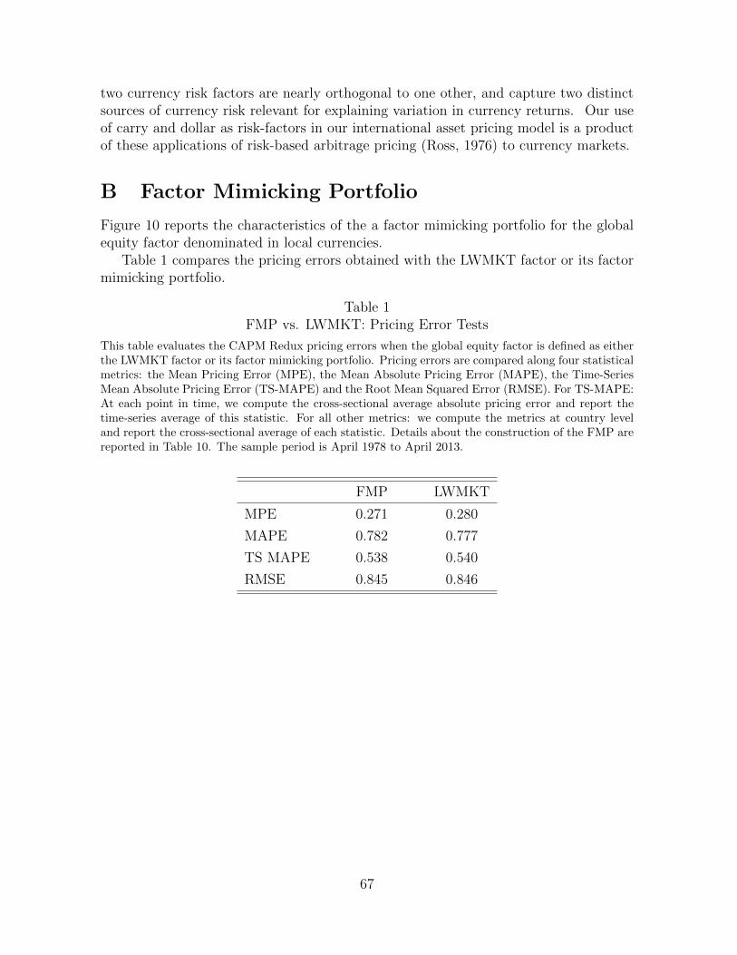
two currency risk factors are nearly orthogonal to one other, and capture two distinctsources of currency risk relevant for explaining variation in currency returns. Our useof carry and dollar as risk-factors in our international asset pricing model is a productof these applications of risk-based arbitrage pricing (Ross, 1976) to currency markets.

B Factor Mimicking Portfolio

Figure 10 reports the characteristics of the a factor mimicking portfolio for the globalequity factor denominated in local currencies.

Table 1 compares the pricing errors obtained with the LWMKT factor or its factormimicking portfolio.

Table 1FMP vs. LWMKT: Pricing Error Tests

This table evaluates the CAPM Redux pricing errors when the global equity factor is defined as eitherthe LWMKT factor or its factor mimicking portfolio. Pricing errors are compared along four statisticalmetrics: the Mean Pricing Error (MPE), the Mean Absolute Pricing Error (MAPE), the Time-SeriesMean Absolute Pricing Error (TS-MAPE) and the Root Mean Squared Error (RMSE). For TS-MAPE:At each point in time, we compute the cross-sectional average absolute pricing error and report thetime-series average of this statistic. For all other metrics: we compute the metrics at country leveland report the cross-sectional average of each statistic. Details about the construction of the FMP arereported in Table 10. The sample period is April 1978 to April 2013.

FMP LWMKT

MPE 0.271 0.280

MAPE 0.782 0.777

TS MAPE 0.538 0.540

RMSE 0.845 0.846

67

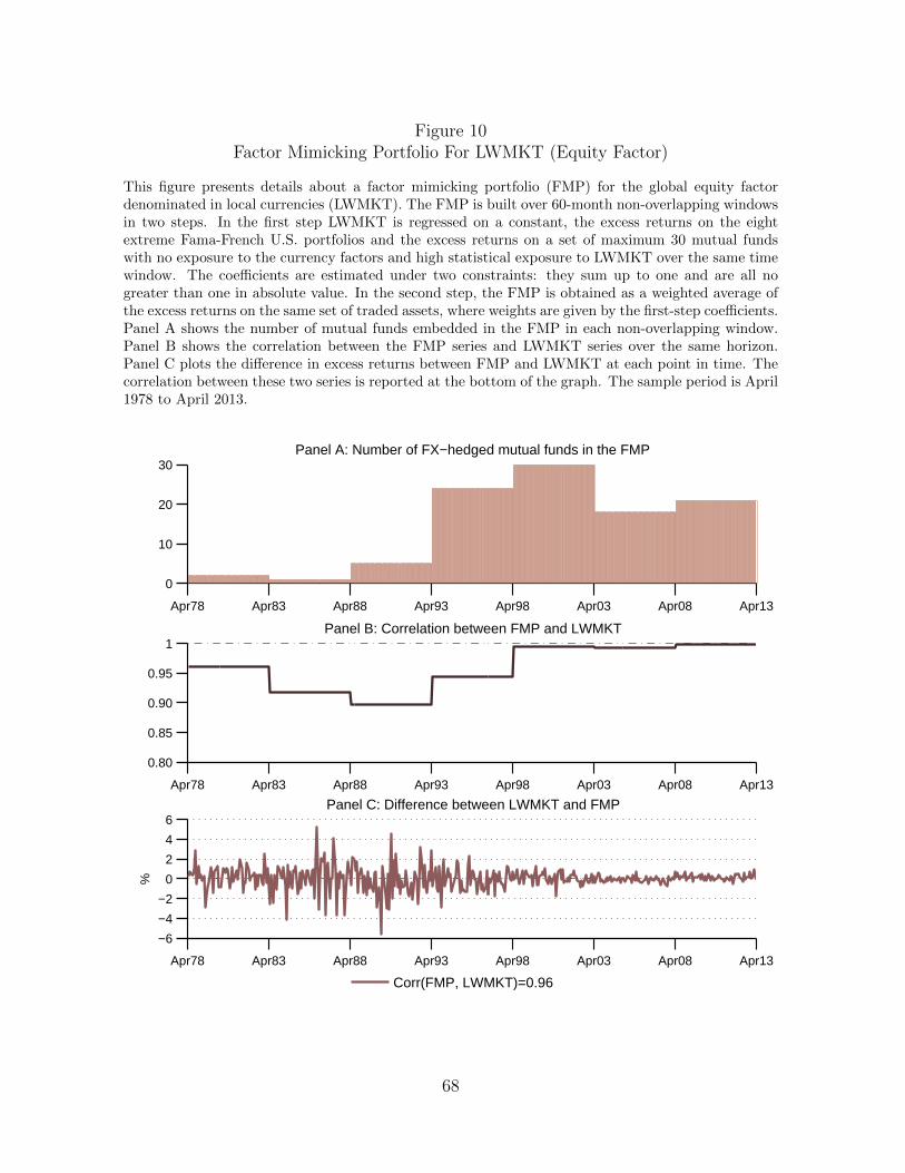
Figure 10Factor Mimicking Portfolio For LWMKT (Equity Factor)

This figure presents details about a factor mimicking portfolio (FMP) for the global equity factordenominated in local currencies (LWMKT). The FMP is built over 60-month non-overlapping windowsin two steps. In the first step LWMKT is regressed on a constant, the excess returns on the eightextreme Fama-French U.S. portfolios and the excess returns on a set of maximum 30 mutual fundswith no exposure to the currency factors and high statistical exposure to LWMKT over the same timewindow. The coefficients are estimated under two constraints: they sum up to one and are all nogreater than one in absolute value. In the second step, the FMP is obtained as a weighted average ofthe excess returns on the same set of traded assets, where weights are given by the first-step coefficients.Panel A shows the number of mutual funds embedded in the FMP in each non-overlapping window.Panel B shows the correlation between the FMP series and LWMKT series over the same horizon.Panel C plots the difference in excess returns between FMP and LWMKT at each point in time. Thecorrelation between these two series is reported at the bottom of the graph. The sample period is April1978 to April 2013.

Apr78 Apr83 Apr88 Apr93 Apr98 Apr03 Apr08 Apr13

0

10

20

30Panel A: Number of FX−hedged mutual funds in the FMP

Apr78 Apr83 Apr88 Apr93 Apr98 Apr03 Apr08 Apr13

0.80

0.85

0.90

0.95

1Panel B: Correlation between FMP and LWMKT

Apr78 Apr83 Apr88 Apr93 Apr98 Apr03 Apr08 Apr13

−6

−4

−2

0

2

4

6Panel C: Difference between LWMKT and FMP

%

Corr(FMP, LWMKT)=0.96

68

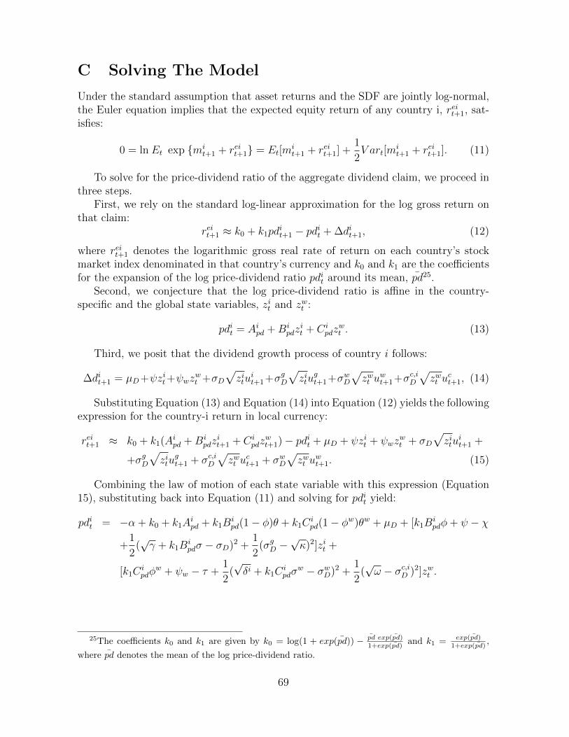
C Solving The Model

Under the standard assumption that asset returns and the SDF are jointly log-normal,the Euler equation implies that the expected equity return of any country i, reit+1, sat-isfies:

0 = ln Et exp mit+1 + reit+1 = Et[m

it+1 + reit+1] +

1

2V art[m

it+1 + reit+1]. (11)

To solve for the price-dividend ratio of the aggregate dividend claim, we proceed inthree steps.

First, we rely on the standard log-linear approximation for the log gross return onthat claim:

reit+1 ≈ k0 + k1pdit+1 − pdit + ∆dit+1, (12)

where reit+1 denotes the logarithmic gross real rate of return on each country’s stockmarket index denominated in that country’s currency and k0 and k1 are the coefficientsfor the expansion of the log price-dividend ratio pdit around its mean, pd25.

Second, we conjecture that the log price-dividend ratio is affine in the country-specific and the global state variables, zit and zwt :

pdit = Aipd +Bipdz

it + Ci

pdzwt . (13)

Third, we posit that the dividend growth process of country i follows:

∆dit+1 = µD+ψzit+ψwzwt +σD

√zitu

it+1+σgD

√zitu

gt+1+σwD

√zwt u

wt+1+σc,iD

√zwt u

ct+1, (14)

Substituting Equation (13) and Equation (14) into Equation (12) yields the followingexpression for the country-i return in local currency:

reit+1 ≈ k0 + k1(Aipd +Bipdz

it+1 + Ci

pdzwt+1)− pdit + µD + ψzit + ψwz

wt + σD

√zitu

it+1 +

+σgD√zitu

gt+1 + σc,iD

√zwt u

ct+1 + σwD

√zwt u

wt+1. (15)

Combining the law of motion of each state variable with this expression (Equation15), substituting back into Equation (11) and solving for pdit yield:

pdit = −α + k0 + k1Aipd + k1B

ipd(1− φ)θ + k1C

ipd(1− φw)θw + µD + [k1B

ipdφ+ ψ − χ

+1

2(√γ + k1B

ipdσ − σD)2 +

1

2(σgD −

√κ)2]zit +

[k1Cipdφ

w + ψw − τ +1

2(√δi + k1C

ipdσ

w − σwD)2 +1

2(√ω − σc,iD )2]zwt .

25The coefficients k0 and k1 are given by k0 = log(1 + exp(pd)) − pd exp(pd)

1+exp(pd)and k1 = exp(pd)

1+exp(pd),

where pd denotes the mean of the log price-dividend ratio.

69

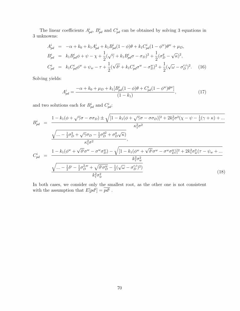
The linear coefficients Aipd, Bipd and Ci

pd can be obtained by solving 3 equations in3 unknowns:

Aipd = −α + k0 + k1Aipd + k1B

ipd(1− φ)θ + k1C

ipd(1− φw)θw + µD,

Bipd = k1B

ipdφ+ ψ − χ+

1

2(√γ + k1B

ipdσ − σD)2 +

1

2(σgD −

√κ)2,

Cipd = k1C

ipdφ

w + ψw − τ +1

2(√δi + k1C

ipdσ

w − σwD)2 +1

2(√ω − σc,iD )2. (16)

Solving yields:

Aipd =−α + k0 + µD + k1[Bi

pd(1− φ)θ + Cipd(1− φw)θw]

(1− k1), (17)

and two solutions each for Bipd and Ci

pd:

Bipd =

1− k1(φ+√γσ − σσD)±

√[1− k1(φ+

√γσ − σσD)]2 + 2k2

1σ2(χ− ψ − 1

2(γ + κ) + ...

κ21σ

2√...− 1

2σ2D +√γσD − 1

2σg2D + σgD

√κ)

κ21σ

2,

Cipd =

1− k1(φw +√δiσw − σwσwD)−

√[1− k1(φw +

√δiσw − σwσwD)]2 + 2k2

1σ2w(τ − ψw + ...

k21σ

2w√

...− 12δi − 1

2σ2,wD +

√δiσwD − 1

2(√ω − σc,iD )2)

k21σ

2w

(18)

In both cases, we consider only the smallest root, as the other one is not consistentwith the assumption that E[pdi] = pdi .

70

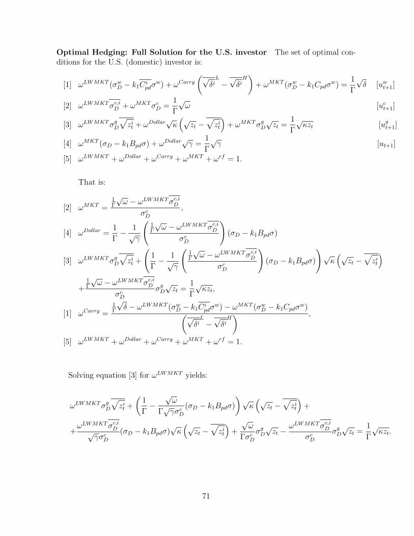
Optimal Hedging: Full Solution for the U.S. investor The set of optimal con-ditions for the U.S. (domestic) investor is:

[1] ωLWMKT (σwD − k1Cipdσ

w) + ωCarry(√

δiL

−√δiH)

+ ωMKT (σwD − k1Cpdσw) =

1

Γ

√δ [uwt+1]

[2] ωLWMKTσc,iD + ωMKTσcD =1

Γ

√ω [uct+1]

[3] ωLWMKTσgD√zit + ωDollar

√κ(√

zt −√zit

)+ ωMKTσgD

√zt =

1

Γ

√κzt [ugt+1]

[4] ωMKT (σD − k1Bpdσ) + ωDollar√γ =

1

Γ

√γ [ut+1]

[5] ωLWMKT + ωDollar + ωCarry + ωMKT + ωrf = 1.

That is:

[2] ωMKT =1Γ

√ω − ωLWMKTσc,iD

σcD,

[4] ωDollar =1

Γ− 1√γ

(1Γ

√ω − ωLWMKTσc,iD

σcD

)(σD − k1Bpdσ)

[3] ωLWMKTσgD√zit +

(1

Γ− 1√γ

(1Γ

√ω − ωLWMKTσc,iD

σcD

)(σD − k1Bpdσ)

)√κ(√

zt −√zit

)+

1Γ

√ω − ωLWMKTσc,iD

σcDσgD√zt =

1

Γ

√κzt,

[1] ωCarry =1Γ

√δ − ωLWMKT (σwD − k1Ci

pdσw)− ωMKT (σwD − k1Cpdσ

w)(√δiL

−√δiH) ,

[5] ωLWMKT + ωDollar + ωCarry + ωMKT + ωrf = 1.

Solving equation [3] for ωLWMKT yields:

ωLWMKTσgD√zit +

(1

Γ−√ω

Γ√γσcD

(σD − k1Bpdσ)

)√κ(√

zt −√zit

)+

+ωLWMKTσc,iD√

γσcD(σD − k1Bpdσ)

√κ(√

zt −√zit

)+

√ω

ΓσcDσgD√zt −

ωLWMKTσc,iDσcD

σgD√zt =

1

Γ

√κzt.

71

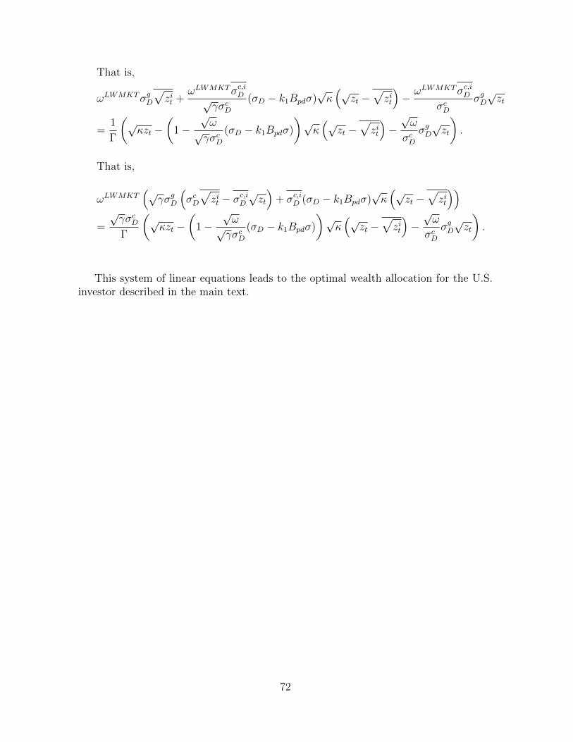
That is,

ωLWMKTσgD√zit +

ωLWMKTσc,iD√γσcD

(σD − k1Bpdσ)√κ(√

zt −√zit

)− ωLWMKTσc,iD

σcDσgD√zt

=1

Γ

(√κzt −

(1−

√ω

√γσcD

(σD − k1Bpdσ)

)√κ(√

zt −√zit

)−√ω

σcDσgD√zt

).

That is,

ωLWMKT(√

γσgD

(σcD√zit − σ

c,iD

√zt

)+ σc,iD (σD − k1Bpdσ)

√κ(√

zt −√zit

))=

√γσcDΓ

(√κzt −

(1−

√ω

√γσcD

(σD − k1Bpdσ)

)√κ(√

zt −√zit

)−√ω

σcDσgD√zt

).

This system of linear equations leads to the optimal wealth allocation for the U.S.investor described in the main text.

72