NBER WORKING PAPER SERIES

THE INTEREST RATE EFFECT ON PRIVATE SAVING:ALTERNATIVE PERSPECTIVES

Joshua AizenmanYin-Wong Cheung

Hiro Ito

Working Paper 22872http://www.nber.org/papers/w22872

NATIONAL BUREAU OF ECONOMIC RESEARCH1050 Massachusetts Avenue

Cambridge, MA 02138November 2016

Aizenman and Ito gratefully acknowledge the financial support of faculty research funds of University of Southern California and Portland State University. Cheung gratefully acknowledges the Hung Hing Ying and Leung Hau Ling Charitable Foundation (孔慶熒及梁巧玲慈善基金)for their support through the Hung Hing Ying Chair Professorship of International Economics (孔慶熒講座教授(國際經濟)). The views expressed herein are those of the authors and do notnecessarily reflect the views of the National Bureau of Economic Research.

NBER working papers are circulated for discussion and comment purposes. They have not been peer-reviewed or been subject to the review by the NBER Board of Directors that accompanies official NBER publications.

© 2016 by Joshua Aizenman, Yin-Wong Cheung, and Hiro Ito. All rights reserved. Short sections of text, not to exceed two paragraphs, may be quoted without explicit permission provided that full credit, including © notice, is given to the source.

The Interest Rate Effect on Private Saving: Alternative PerspectivesJoshua Aizenman, Yin-Wong Cheung, and Hiro ItoNBER Working Paper No. 22872November 2016JEL No. F3,F41,F42

ABSTRACT

Using an uneven panel of 135 countries from 1995 to 2014, we investigate the link between interest rates and private saving, and focus on whether the interest rate effect is dominated by the income (i.e., negative) or the substitution (i.e., positive) effect. With the baseline estimation, we find that the real interest rate has the substitution effect on private saving only for a full-country sample and a group of Asian economies. We also examine if low real - or nominal - interest rates have any impact on the link between the real interest rate and the private saving rate. We find that among developing countries, when the nominal interest rate is not too low, we detect the substitution effect of the real interest rate on private saving. However, among industrial and emerging economies, the substitution effect is detected only when the nominal interest rate is lower than 2.5%. In contrast, emerging-market Asian countries are found to have the income effect when the nominal interest rate is below 2.5%. When we examine the interactive effects between the real interest rate and the variables for economic conditions and policies, we find that the real interest rate has a negative impact - i.e., income effect - on private saving if any output volatility, old dependency, or financial development is above a certain threshold. Further, when the real interest rate is below 1.5%, greater output volatility would lead to higher private saving in developing countries. Lastly, we find that old dependency ratios, public healthcare expenditure, and financial development have negative impacts on private saving, but such impacts in absolute values tend to become smaller as the real interest rate becomes lower.

Joshua AizenmanEconomics and SIRUSCUniversity ParkLos Angeles, CA 90089-0043and NBERaizenman@usc.edu

Yin-Wong CheungDepartment of Economics and FinanceCity University of Hong KongHong Kongyicheung@cityu.edu.hk

Hiro ItoPortland State University1721 SW Broadway, Suite 241Portland, Oregon 97201ito@pdx.edu

2

1. Introduction

In the summer of 2014, when the European Central Bank changed its interest rate on

excess bank reserves to -0.1%—a negative policy interest rate for the first time in not only its own

history but also in the history of major central banks—advanced economies implementing

unconventional monetary policies entered a new phase.1 Eighteen months later, this action was

followed by the Bank of Japan’s decision to adopt negative interest rates. As of the fall 2016, 19

euro countries, plus Japan, Denmark, Sweden, and Switzerland, have adopted negative policy

interest rates.

As unconventional actions often face opposition in general, negative interest-rate policies

have also faced challenges against their effectiveness. Conventionally speaking, lower interest-

rate monetary policy is supposed to encourage present-day consumption (as opposed to future

consumption), by lowering the rewards for postponing consumption. More simply, lowering the

policy interest rate is expected to stimulate consumption and investment while discouraging people

to save. Expected as a further drastic action, negative interest rates would not just discourage, but

also penalize people if they postpone consumption. Hence, conceptually, negative interest rates

may lead people to spend now rather than later and therefore discourage saving.

Recently, debates have proliferated regarding the effectiveness of negative interest-rate

policy. Some people have argued that negative interest rates may not work as central bankers

expect.

As for the link between the interest rate and saving, the argument is as follows: lower or

negative interest rates may contribute to higher, not lower, saving rates because the rate of return

per financial instrument is so low that people may try to compensate by increasing their aggregate

1 As an exception, Denmark had lowered its benchmark rate to a negative figure in mid-2012. Another exception is Switzerland, which levied negative interest rates on CHF deposits from non-residents in 1972 to curb rapid capital inflows. This policy lasted until 1978.

3

amount of saving. This scenario can be especially true in an economy with an aging population, as

people might want to target their saving to be better prepared for retirement. Such a tendency can

also be strong in an economy in which sufficient social protections such as social securities and

unemployment benefits are not available. Generally, people may want to increase their aggregate

amount of saving in response to lower interest rates if they face a gloomy and more volatile

economic outlook. Thus, the behavior of precautionary saving may change depending on economic

or policy conditions.

This is not just an issue for advanced economies with low or negative interest rates, but

for developing economies as well. In fact, in a developing economy with financial repression,

nominal interest rates tend to be artificially repressed and therefore the real rates of return tend to

be low. This situation can be exacerbated if the economy of concern experiences high inflation. If

such an economy is also coupled with underdeveloped public social-protection programs, people

have reason to increase the aggregate amount of saving for precautionary purposes.

While the interest rate effect on private saving is commonly perceived to be positive,

Nabar (2011) notes that China experienced a combination of rising household saving and declining

real interest rates during the 2000s. Using province-level data over the 1996–2009 period, Nabar

empirically shows that when the return to saving declines, household saving rises.

Is China’s documented interest-rate-saving link an isolated instance or an example of the

negative income effect of the interest rate? To shed some light on this question, we employ a panel

of countries to conduct an extensive empirical study on the link between interest rates and private

saving. At the outset, we recognize that the interest rate effect on private saving can be ambiguous.

As noted earlier, low interest rates can discourage saving because of the substitution effect, or

conversely, encourage saving via the income effect to achieve, say, a targeted saving goal.

Because of the conflicting channels, the observed or final effect of the interest rate on

4

saving can depend upon the level of the interest rate itself as well as on other contributing factors.

In an environment in which the interest rate is extremely low, the income effect may, for example,

outweigh the substitution effect. In other words, in such an environment, agents may be worried

about the possibility of not meeting financial investment objectives such as retirement, and

therefore try to overcome the low return by increasing the aggregate volume of saving. In this case,

lower interest-rate levels would lead to higher levels of saving. Or, the effect of the interest rate on

saving may differ depending on macroeconomic or demographical conditions or policy

environment.

Examining the link between the interest rate and saving is important. In the short term,

whether policy interest rates and saving rates have a positive or negative relationship also refers to

the kind of impact a monetary policy would have on consumption and is therefore related to the

question of stabilization measures.

Furthermore, this issue is also important in the context of the global imbalance debate. In

the years leading up to the Global Financial Crisis of 2008, many emerging market economies in

East Asia (most notably China) and oil exporters persistently ran current-account surpluses during

the global trend of lower real interest rates. Some economists argue that high savings in rapidly

growing emerging markets are responsible for such current account surpluses and thus contributing

to global economic instability (Greenspan, 2005a, b, and Bernanke, 2005). Hence, investigating

how an ultra-low-interest rate environment would contribute to saving on a global scale is

important.

In the long term, the impact of the interest rate on saving is related to the question of

capital accumulation, which would determine future income level and thereby present-day

consumption and saving. Thus, the nature of the interest-rate-saving link can be an important

determinant for the sustainability of long-term economic development.

5

Therefore, we investigate whether the interest rate has the income (i.e., negative) effect or

the substitution (i.e., positive) effect on private saving by using panel data of 135 countries over

the 1995–2014 period while controlling for other factors that can affect the behavior of private

saving. Furthermore, we will empirically examine whether and how the impact of the interest rate

on saving can be affected by economic, demographical, and policy conditions.

In the next section, we introduce potential determinants of private saving and discuss their

impacts. In the same section, we present some stylized facts of private saving and the real interest

rates to show general trends of these variables. In Section 3, we introduce our estimation model

and discuss the results from the baseline estimations. We extend our analysis and examine whether

any interactive effects exist between the real interest rate and other macroeconomic and structural

conditions in Section 4. In this section, we also discuss the implications of our estimation results

for Asian economies and several advanced economies. In Section 5, we offer concluding remarks.

2. Theory and Evidence about Private Saving

2.1 What Kind of Saving Do We Focus On?

A large number of studies have investigated the determinants of saving; a sample of these

studies include Masson et al. (1998), Loayza et al. (2000a, 2000b), Aizenman et al. (2015), and

Aizenman and Noy (2013). Since these studies have provided comprehensive reviews on theory

and empirical evidence pertaining to the determinants of saving, we focus on the theoretical

predictions of the factors relevant to our empirical analysis.

Before introducing potential determinants of saving, we need to clarify the kind of saving

we are referring to. In this paper, we consider private saving, which we define as the difference

between domestic saving and public saving. Considering that our interest is to assess the relative

importance of income and substitution effects on shaping the interest-rate impact on saving, it

6

would have been ideal if we had been able to focus on household saving.

However, we have two reasons for avoiding using household saving data—one conceptual

and the other practical. First, in a practical sense, household saving data are extremely limited.

One reason for this scarcity is that household saving data are typically derived from government

surveys that could be based on a wide variety of methods across countries (and over time). Even

if we had a uniform survey method, disagreements could arise over what to include in consumption,

saving, or disposable income when calculating the saving rate. For example, the question exists

whether capital gains from financial investments should be included in saving or disposal income,

or both. Similar concerns arise for social security payments, or depreciation of household assets in

saving or income. Depending on the methodologies of data construction, there can be a wide

variety of household saving.2 Different types of household saving data exist for different countries.

Also, the type of items that should be included in saving and income to compute the saving rate

depends on the aspect of saving behavior a researcher chooses to study. Hence, a data set of

household saving rate that is consistently compiled is hard to obtain. Although the OECD publishes

consistent household saving data for 33 countries, the data are mostly composed from advanced

economies.

There is also a conceptual reason that makes it difficult to use household saving data. The

line between household and corporate saving, which sum up to define private saving, can be blurry.

This issue is prevalent among developing countries because of the existence of vast informal labor

markets that make it difficult to separate corporate income from household income and vice versa.

To a certain extent, there are also difficulties in disentangling household, corporate income, and

consumption in advanced economies.

2 There can also be gross or net household saving. See Audenis et al. (2004) for details.

7

Hence, we focus on private saving as a share of GDP, in which we obtain the amount of

private saving by subtracting the general government-budget balance from domestic saving while

assuming the latter equals the sum of household, corporate, and public savings.

2.2 Theoretical Predictions of the Determinants of Private Saving

We now discuss the theories underlying the determinants of private saving and, hence, the

expected signs of estimated coefficients in the following empirical analysis.

Persistence: Considering that economic agents usually try to smooth their consumption,

private saving should also be smoothed out, and therefore, it tends to be serially correlated. Also,

the determinants of private saving can have impact with some time lags; thus, private saving tends

to show inertia. A number of empirical studies include the lagged dependent variable as one of the

explanatory variables, and the lagged dependent variable tends to be highly significant with

relatively large magnitudes.

Public saving: The theory of Ricardian equivalence predicts that, in a world where tax

policy creates no distortion, any change in public saving can be offset exactly by the same but

opposite change in private saving, which makes its estimate negative with a magnitude of one.

However, empirical studies usually show that a full offset is not existent, but that a partial offset is

often prevalent, with the average absolute estimate ranging 0.25–0.60.3

Credit growth: If credit constraint is mitigated by credit growth, agents would increase

their consumption, and hence, decrease saving (Loayza et al., 2000a, 2000b). Therefore, we can

expect the estimate on credit growth to be negative. We include the growth rate of private credit

creation (as a share of GDP) as a proxy for credit growth or credit availability.

3 See de Mello et al. (2004).

8

Financial development: Further financial development or deepening could induce more

saving through increased depth and sophistication of the financial system. As a contrasting view,

more developed financial markets lessen the need for precautionary saving and thereby lower the

saving rate. Thus, the predicted sign of the estimate for the financial development variable is

ambiguous. We use private credit creation (as a share of GDP) as a proxy for financial development.

Financial openness: The impact of financial openness on saving behavior can also be

explained similarly to that of financial development. To measure the extent of financial openness,

we use the Chinn-Ito index (2006, 2008) of capital account openness.4

Both financial development and financial openness could affect the level of private saving

through the price channel. That is, financial development and liberalization usually mitigates

financial repression, in which the interest rate tends to be artificially depressed due to regulatory

controls and lack of competition. Once financial repression is mitigated, higher interest rates can

prevail and affect private saving, although the effect of interest rates on saving can be ambiguous.

We can expect, at the very least, to see interactive effects between financial development or

openness and the interest rate.

Output volatility: Risk-averse consumers who face more volatile income flows might set

resources aside for precautionary reasons in order to mitigate unexpected future income shocks

and smooth their consumption streams.5 Hence, generally, we can expect private saving to be

positively correlated with output volatility.6

Income growth: Based on the permanent income hypothesis (Friedman, 1957), higher

income growth, which may represent higher future growth, should lead to higher saving. The life-

4 For both financial development and financial openness, Chinn et al. (2014) find negative effects on national saving. 5 See Skinner (1998), Zeldes (1989), and Hansen and Sargent (2010). 6 Aizenman et al. (2015) focus on empirical evidence that saving rates and output volatility are negatively correlated and provide theoretical explanations.

9

cycle hypothesis (Modigliani and Brumberg, 1954) is vague on such a link, making it conditional

on other factors including credit constraint. Vast empirical literature has shown that income levels

are positively correlated with saving.

Demography: The life-cycle hypothesis (Friedman, 1957) shows that demographical

distribution of the population affects saving behavior. Both young and old populations tend to

dissave while the working population tends to save to both pay off past debt and prepare for

retirement life.

Per capita income level (in PPP): The stage of development, as well as demographic

characteristics, should also affect saving behavior. Highly developed economies may live on

savings from periods when they were high-growth economies and thus the impact of economic

development can be negative. However, both the permanent income hypothesis (Friedman, 1957)

and the lifetime-cycle hypothesis (Modigliani and Brumberg, 1954) predict that the impact of

income shocks on consumption—i.e., saving—depends on whether the shocks are temporary or

permanent. Although temporary positive shocks to income would lead merely to an increase in

saving but no change in consumption, permanent shocks might lead to an increase in consumption,

that is, a decrease in saving.7 In either case, per capita income should lead positively to saving

based on these hypotheses. Furthermore, more practically, a measure of per capita income can be

highly correlated with the level of institutional or legal development. Economies with more

developed institutions or legal systems can provide a friendly environment for saving, which also

suggests a positive impact of income level. Thus, the predicted sign of a measure of economic

development should be ambiguous.

Interest rates: The effect of the interest rate on saving is equivocal. Theoretically, although

7 Obstfeld and Rogoff (1996) formalized the prediction in a simple intertemporal trade setting.

10

the interest rate means the real interest rate, the nominal interest rate has tended to be in the

spotlight in recent years.8 On the one hand, changes in the interest rate could have a substitution

effect on saving; for example, the lower the interest rate, the higher the level of consumption—i.e.,

leading to a lower level of saving. On the other hand, changes in the interest rate could have an

income effect. In other words, the lower the interest rate, the higher the expected level of saving,

because the lower rate of return from investment must be compensated by a higher saving rate.

Hence, the predictive power of the interest rate and its sign depends on the relative magnitude of

income and substitution effects.

Masson et al. (1998) find a positive effect of interest rates on saving while Loayza et al.

(2000b) find a negative effect. Nabar (2011) uses provincial data in which an increase in urban

saving rates in China is negatively associated with a decline in real interest rates in the 1996– 2009

period.

2.3 Stylized Facts

Before formally investigating the impact of candidate determinants on private saving, we

would like to grasp the general trends of private saving and the real interest rate.

Figure 1 illustrates the development of private saving (as a share of GDP) over the last

two decades for several country groups and selected individual countries. In Panel (a), country

grouping is based on income levels while Panel (b) compares the group of emerging market

economies in Asia excluding China (ex-China EMG Asia) and Latin American economies with the

U.S., the euro area, China, and Japan.

Interestingly, the private saving rates are comparable between the groups of industrialized

8 We use the real interest rate that is calculated as: ln . See the data appendix for details.

11

countries (IDC) and the emerging market economies (EMG), while the group of developing

countries excluding EMG (Non-EMG LDC) has much lower saving rates. In the 1995–2005 period,

the saving rates of both EMG and non-EMG LDC appear relatively stable, while IDCs’ saving rate

falls in the late 1990s and rebounds in the early 2000s. IDCs’ private saving rates start rising again

in 2007, followed by EMG in 2008, with both peaking in 2010. Considering the mortgage crisis in

the U.S. and Europe in 2007 and the 2008 GFC, one interpretation is that people increased their

savings in response to heightened economic uncertainty, which was accompanied with falls in

interest rates.

When we compare individual economies and regional groups of economies (Panel (b)),

China, with high saving rates, appears as an outlier—a fact that has been documented by many

observers. China is followed, with some gaps, by other emerging Asian market economies. The

U.S. also appears distinct with its low saving rates, whereas Japan’s saving rate has been declining

over the last two decades. All individual economies or country groups appear to have experienced

a discrete rise in saving rates in 2009, followed by a moderate fall in the last five years of the

sample.

We illustrate the evolution of the real interest rate along with the nominal interest rate and

the inflation rate in Figure 2.

From the late 1990s through the mid-2000s, many countries have experienced persistent

declines in the real interest rates. Both panels on the top row show that the real interest rates have

been converging throughout that period. At the same time, the nominal interest rate has continued

to fall while the inflation rate has remained stable. All of these factors point to characteristics of a

Great Moderation. In 2008, the real interest rates fell sharply, which reflected a sharp rise in

inflation mostly due to high energy prices, as well as sharp drops in the nominal interest rates that

were implemented as stabilization measures in response to the GFC. In the post-GFC period,

12

advanced economies implemented the zero interest-rate policy, which was followed by declines in

the nominal interest rates of developing countries and in EMG. During this period, while the

nominal interest rates remained relatively constant (i.e., constantly low or constantly zero),

inflation rates continuously fell after 2011. All of these factors contributed to a continuous rise in

the real interest rates.

In Figure 3, we compare the correlations of private saving and the real interest rates

between the first five years (i.e., 1995–1999) of the sample period—when the real interest rates

were generally high—and the last five years (i.e., 2010–2015)—when the real interest rates were

generally low.9 The correlation for the full sample is significantly negative for the last five years,

suggesting that the interest rate has had an income effect on private saving, while it is only

insignificantly negative in the first five years. The slopes in the two periods are significantly

different. When we look at the subgroups, the correlation is significantly positive for the EMG

countries in both periods with no significant change in the slope between the two periods. The non-

EMG LDC group has a significantly negative slope only in the last five-year period, which is

significantly different from the first five years. For the IDC group, interestingly, the correlation

becomes positive in the last five-year period, although it is significantly negative in the first period.

Lastly, for the Asian EMG subgroup, the correlation is more significantly negative with a larger

magnitude in the last five years compared to the first period. Overall, there is evidence that the

nature of the correlation has changed over the two periods, and that the correlation becomes more

significantly negative with a larger magnitude for developing countries.

Naturally, there are limits to this kind of exercise with unconditional correlations. Hence,

we implement a more formal empirical analysis in the next section.

9 To exclude outliers, we remove the 2.5 and 97.5 percentiles of private saving and real interest rate observations for each sample. We also remove country years for which the rate of inflation is greater than 40%.

13

3. Baseline Estimation

3.1 Estimation Model

With the above theoretical discussions and stylized facts in mind, we estimate the

determinants of private saving using the empirical specification:

, (1)

where yit is private saving (normalized by GDP); X is a vector of endogenous variables; Z is a

vector of exogenous variables; and rit is the real interest rate. ui refers to unobserved, time-invariant,

country-specific effects, whereas is a time-specific effect variable. is the i.i.d. error term.

Equation (1) entails a few possible technical issues. First, as we have already discussed,

private saving can involve inertia. To allow for persistency in private-saving data, we need to

estimate a dynamic specification that can address both short- and long-term effects of explanatory

variables. Second, some of the explanatory variables can be jointly determined with the saving

rate. Hence, we have to account for joint endogeneity of the explanatory variables. Last, we need

to control for unobserved country-specific effects correlated with the regressors. The system

generalized method of moments (GMM) estimation method, which can consistently estimate a

dynamic panel while allowing for joint endogeneity and controlling for potential biases arising

from country-specific effects, is therefore adopted for our empirical exercise (Arellano and Bond,

1991; Arellano and Bover, 1995; Blundell and Bond, 1998).

In the vector X of endogenous variables, we include public saving (i.e., the general

government budget balance normalized by GDP); financial development that is measured by

private credit creation as a share of GDP; credit growth that is measured by the growth rate of

ittiititititit uZXryy ''110

t it

14

private credit creation; and per capita income. These variables are treated as “internal instruments”

in the GMM estimation. As exogenous variables, vector Z includes young and old dependency

ratios, public healthcare expenditure (as a share of GDP), financial openness, output volatility, and

per capita income growth.

The variable of our focus is the real interest rate r. If the substitution effect outweighs the

income effect, the estimate of β1 is expected to be positive. That is, the higher the interest rate, the

more the country would save. On the other hand, if the income effect outweighs the income effect,

β1 would be negative; that is, the higher the interest rate, the less private saving.

3.2 Estimation Results

Table 1 reports the results of the estimations for the full sample and the subsamples of

industrialized countries (IDC), less developing countries (LDC), emerging market countries

(EMG), Latin American EMG (LATAM EMG), Asian economies, (Asia), and the emerging market

countries in Asia (Asian-EMG).

Before discussing the system GMM estimates, we conduct diagnostic tests for the

validity of the instruments and serial correlation in estimated residuals. For the former, we conduct

the Hansen-J test against the null hypothesis that the instrumental variables are uncorrelated with

the residuals. If the test fails to reject the null hypothesis, the specification is free of the issue of

over-identification. As for serial correlation, we conduct an AR(2) test with the null hypothesis

that the errors in the differenced equation exhibit no second-order correlation. This is because the

system GMM method involves a first-difference transformation of the original estimation model

to eliminate the unobserved country-specific effect.

The estimated system GMM model specification is supported if no evidence exists of

second-order autocorrelation (even there is first-order autocorrelation) and the over-identifying

15

restrictions are not rejected at conventional levels of confidence.

In Table 1 and the other tables, the reported diagnostic test results—both the Hansen-J

and AR(2) test results—support the use of the system GMM model specification for all of these

samples. That is, the Hansen test fails to reject the null hypothesis of over-identifying restrictions,

and the AR(2) test confirms that the estimated errors in the differenced equation exhibit no second-

order correlation.10

Generally, the estimation results are consistent with our theoretical discussions.

First, the real interest rate, the variable of our focus, enters the estimation significantly

for the full sample and the subsample of Asian economies group with a positive sign. This means

we detect that the substitution effect outweighs the income effect for these groups of countries. For

the other samples, the estimates are positive, except in the cases of LATAM and Asian EMG, which

are not significant.

The behavior of private saving is found to be somewhat persistent. The degree of

persistency is 0.390 for the full sample, although this varies across different subsamples. The

groups of Asian economies and Asian EMG have higher degrees of persistency, which is consistent

with the prevailing observation that Asian economies’ saving rates are consistently high.

We can observe evidence for the partial Ricardian offset. The results of the full sample

indicate that about 44% of an improvement in public saving would be offset by a worsening of

private saving. The size of the offset is much larger among industrialized countries than in

10 However, Roodman (2006) argues that including too many instruments cannot only overly fit endogenous variables, but also weaken the power of the Hansen test to detect over-identification. He suggests that high p-values (such as “1.00”) for the Hansen test may signal that the test wrongly failed to detect over-identification. In fact, in Table 1 and others, we see that the smaller the sample (such as IDC, EMG, and regional country groups), the more tendency for the Hansen test’s p-value to take the value of “1.00.” This can be related to the fact that in a smaller sample, N (= the number of countries) tends to be small relatively to T (= the number of years)—the GMM estimation is more suitable for a data set with the dimension of large N and small T. However, when we apply the random effect model (not reported), the estimation results are qualitatively intact; in fact, they tend to become more robust. Hence, we focus on discussing the results from the GMM estimations.

16

developing economies, which may be because the tax system in the former is less distortive than

in the latter.

While the level of financial development only matters for industrialized economies,

credit growth is found to be a negative contributor for developing economies. Once credit

conditions improve, a developing country tends to experience growth in its consumption—that is,

a fall in its saving rate.

Financial openness, in contrast, is a positive contributor, although only for the IDC and

the LATAM EMG. For these economies, financial openness helps increase private saving through

increasing investment opportunities.

Although both the level and the growth of per capita income are found to positively

contribute to private saving, output volatility has opposing effects for developed countries and the

group of Asian-EMG economies.

The higher the country’s level of old dependency, the lower the rate of private saving it

tends to experience. Although the estimate on the old dependency variable is not significant for

the LDC or EMG group, the estimates for the subgroups of LATAM, Asia, and Asian-EMG are

significant and their magnitudes tend to be large. However, smaller numbers of countries are

included in each of the estimations, which indicate that demographical change happened rather

drastically in the sample period and had significant impact on private saving for the countries in

these subsamples.

Healthcare expenditure, which we measure by public health expenditure as a share of

GDP, has a negative impact on private saving. That is, if healthcare is more readily available with

the support of the public sector, people reduce saving because they would not have to save for

precautionary reasons. The estimate is robust across the different country groups based on income

levels (i.e., full, IDC, LDC, and EMG). Also, when we use social expenditure as a share of GDP

17

that is available in the OECD database, the results are essentially unchanged.11

We also test property prices and net (foreign) investment as potential determinants of

private savings.

A rise in house prices could create a “wealth effect” on consumption while

simultaneously mitigating credit constraint. Either way, we expect property prices to have a

negative impact on saving. We find such a negative impact only for EMG (Appendix 3, Table

A1).12 However, when we test the growth-rate impact of property prices, we find that its estimate

is significantly negative for the full sample and the LDC subgroup (Table A2). In these samples,

what matters is not so much the level of property prices as its growth rate. A rapid rise in property

prices may signal an increase in future or permanent income flows.

Another determinant of our concern is net investment position. Foreign saving can either

complement domestic private saving or crowd out domestic private saving. Facing credit constraint

domestically, developing countries often try to import foreign saving. However, they also have to

face external borrowing constraints, such as difficulties in borrowing in their own currencies or

for the long terms (i.e., the “original sin” argument). In fact, Aizenman et al. (2007) estimate that

only 10% of the capital stock in developing countries is funded with foreign saving, which means

that 90% is self-financed.13

We test whether net investment positions affect the private saving rate by including a

dummy for country-years in which the net position is negative.14 The estimation results (Table

11 The data are available only for OECD countries as well as for 1980, 1985, 1990, 1995, 2000, 2005, and 2009–2014. 12 Nabar (2011) and Geerolf and Grjebine (2013) find similar results. 13 They also show that countries with higher self-financing ratios grew significantly faster than countries with low self-financing ratios. 14 For the dummy variable, we use the data of external assets and liabilities from the Lane-Ferretti data set (2001, 2007, updates). We use this data set because we find that the net investment position as a share of GDP does not have a significant impact for all the samples. This insignificant result is not surprising given that the data for financial center countries (e.g., Ireland, Hong Kong, Singapore) and heavily indebted countries can be outliers affecting the estimation results.

18

3A) show that the saving rate tends to be lower for net debt countries, which means foreign saving

complements domestic saving.

3.2.1 Level Impacts of the Interest Rates

The weak evidence of the real interest-rate effect in Table 1 is likely to be attributable to

its dependency on other economic conditions affecting the saving decision. Our sample period, for

instance, includes the GFC and consequential implementations of unconventional monetary policy

by advanced economies, such as quantitative easing and negative interest-rate policies. These

unconventional monetary policies were implemented primarily in response to financial instabilities

experienced by the U.S. and several euro member countries. However, these policies also created

repercussions among emerging market economies through surges of capital flows triggered by

extremely low rate of returns in advanced economies and now possible retrenchment of such flows

due to U.S. monetary contraction, which began in late 2015. Thus, spillovers of the GFC and

unconventional monetary policy heightened the level of uncertainty among advanced economies

as well as emerging market economies, which may have impacted saving behavior. More

specifically, low interest rates may signal future monetary uncertainty or financial condition

uncertainty and thereby encourage people toward precautionary saving.

Against this backdrop, we examine whether low real- or nominal-interest rates have any

impact on the link between the real interest rate and the private saving rate.

The estimation model shown below includes the interaction between the real interest rate

and the dummy for a certain threshold of the real or nominal interest rate. In the following

regression equation, D takes a value of one when the interest rate of concern is below a certain

threshold; that is D = I (interest rate < threshold value),

19

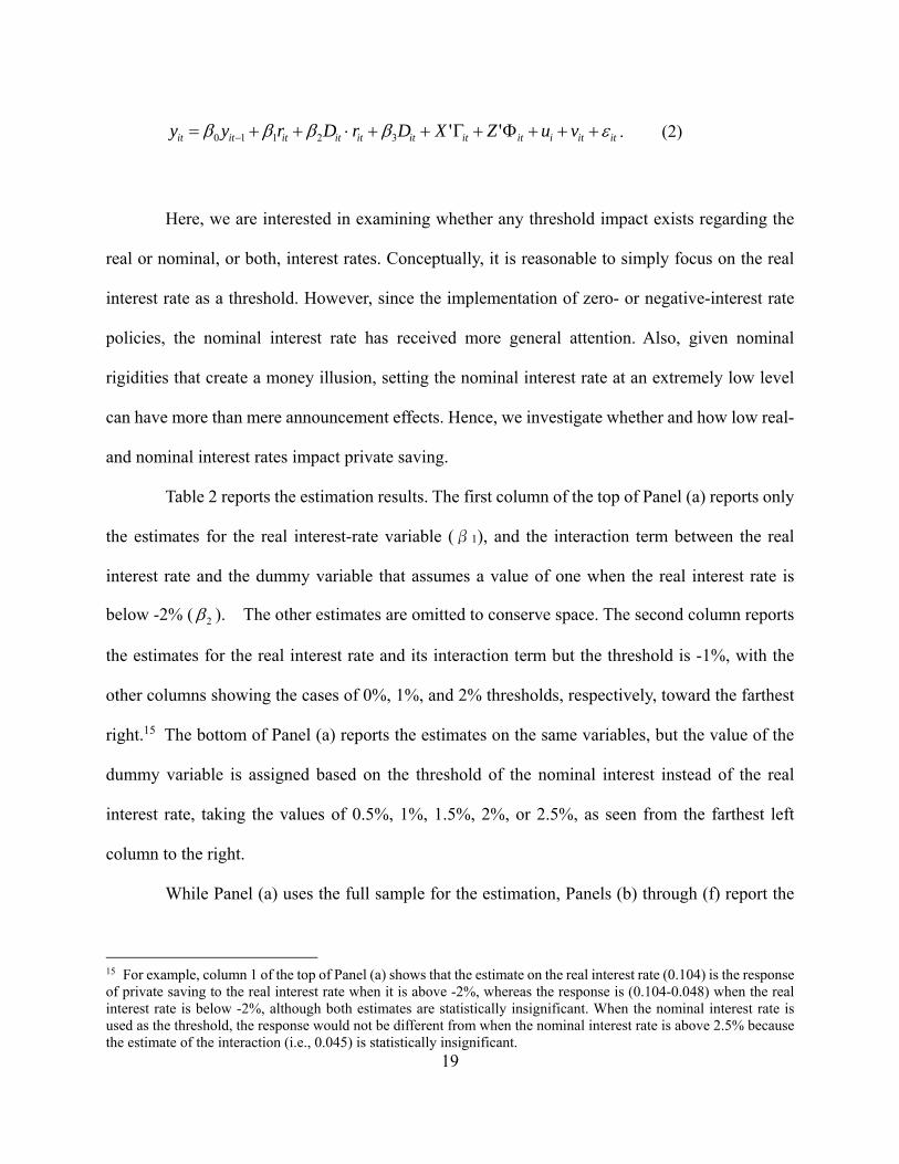
ititiitititititititit vuZXDrDryy ''32110 . (2)

Here, we are interested in examining whether any threshold impact exists regarding the

real or nominal, or both, interest rates. Conceptually, it is reasonable to simply focus on the real

interest rate as a threshold. However, since the implementation of zero- or negative-interest rate

policies, the nominal interest rate has received more general attention. Also, given nominal

rigidities that create a money illusion, setting the nominal interest rate at an extremely low level

can have more than mere announcement effects. Hence, we investigate whether and how low real-

and nominal interest rates impact private saving.

Table 2 reports the estimation results. The first column of the top of Panel (a) reports only

the estimates for the real interest-rate variable (β1), and the interaction term between the real

interest rate and the dummy variable that assumes a value of one when the real interest rate is

below -2% ( 2 ). The other estimates are omitted to conserve space. The second column reports

the estimates for the real interest rate and its interaction term but the threshold is -1%, with the

other columns showing the cases of 0%, 1%, and 2% thresholds, respectively, toward the farthest

right.15 The bottom of Panel (a) reports the estimates on the same variables, but the value of the

dummy variable is assigned based on the threshold of the nominal interest instead of the real

interest rate, taking the values of 0.5%, 1%, 1.5%, 2%, or 2.5%, as seen from the farthest left

column to the right.

While Panel (a) uses the full sample for the estimation, Panels (b) through (f) report the

15 For example, column 1 of the top of Panel (a) shows that the estimate on the real interest rate (0.104) is the response of private saving to the real interest rate when it is above -2%, whereas the response is (0.104-0.048) when the real interest rate is below -2%, although both estimates are statistically insignificant. When the nominal interest rate is used as the threshold, the response would not be different from when the nominal interest rate is above 2.5% because the estimate of the interaction (i.e., 0.045) is statistically insignificant.

20

results for IDC, LDC, EMG, Asia, and Asian EMG, respectively.

When the estimate ( 2 ) is found to be significant, it would mean that the impact of the

real interest rate on private saving changes when the real or nominal interest rate is below a certain

level.

In Panel (a), in the presence of real interest rate regime variables, there is no evidence of

significant the real interest rate effect ( 1 ). However, when we control for low nominal interest

rate regime, the real interest rate effect becomes significantly positive – the estimated substitution

effect is in accordance with the full sample result in Table 1.16 As far as the full sample is

concerned, low nominal interest rates affect the way the real interest rate affects private saving.

For the subsample of industrialized countries (Panel (b)), the real interest rate has the

substitution effect when the real interest rate is lower than -1% or the nominal interest rate is lower

than 2.5%. In fact, when we test the threshold of 3%, the interaction term is still significant, and it

becomes insignificant at the 3.5% threshold (not reported). For this group of countries, the

substitution effect is dominant but only when the real or nominal interest rate is low.

Results in Panel (c) are quite similar to the results of the full sample. According to the

panel, when the nominal interest rate is above 0.5%, the real interest rate has the substitution effect

on private saving whereas countries with nominal interest rates below 0.5% have stronger

substitution effects.17 These results indicate that, overall, the positive real interest rate effect is the

norm, and the threshold of the nominal interest rate is more relevant than that of the real interest

rate.

16 The dummy for the 0.5% threshold is also significant, but it can be considered as reflecting a “subset” of the dummy for 2.0%. 17 The countries which have the nominal interest rates below 0.5% in this sample include Panama, The Bahamas,

Belize, Trinidad and Tobago, Bahrain, Cyprus, Oman, Qatar, Nepal, Singapore, Algeria, Bulgaria, Czech Republic,

Slovak Republic, Estonia, Latvia, Lithuania, Croatia, and Slovenia in years after the Global Financial Crisis of 2008.

21

When we look at the EMG group, the significant real interest effect appears when the

nominal interest rate is below 2.5%, indicating that when the nominal interest rate is below 2.5%,

the real interest rate has the positive effect on private saving among these economies.18 Also, it is

noted that the magnitude of the effect is quite large.

When we restrict our sample to Asian economies (Panel (e)), we only find that the real

interest rate generally has a substitution effect on private saving. The group of Asian EMG

economies, however, displays a different pattern of real interest rate effects. In Panel (f), the

estimated 2 is now significantly negative for the threshold of 2.5%.19 That is, when the nominal

interest rate is below 2.5%, private saving for Asian EMG would negatively respond to the real

interest rate movement. That is, the income effect outweighs the substitution effect.

4. Interactive Effects

4.1 Empirical Findings

Results in the previous section show that the real interest-rate effect, if significant, tends

to be positive; the substitution effect tends to dominate the income effect. The effect varies across

different country groups, and its magnitude can be influenced by the level of nominal interest rate.

In the case of the Asian EMG group, the real interest-rate effect has become negative when the

nominal interest rate is lower than 2.5%. Overall, these results suggest that the effect of the real

interest rate on private saving can depend on the economic environment at large.

In this section, we use interaction variables to explore the real interest-rate effect under

alternative economic conditions. For example, when an economy experiences a high level of

18 The threshold of 3% is found to be insignificant (not reported).

19 The threshold of 3% is found to be insignificant (not reported).

22

output volatility, a low interest rate can be interpreted as a sign of economic weakness and thus,

can strengthen the saving incentive. Alternatively, for an economy in which old dependency is

increasing, a lowering of the interest rate might encourage people to increase their rates of saving

to reach pre-determined target levels of retirement saving.

In the following, we investigate influences of the economic environment that are captured

by output volatility, old dependency, healthcare expenditure, financial development, and financial

openness on real interest-rate effects. Specifically, we include the term , where is the

economic environment variable under consideration to examine the interactive effect in the

modified saving regression equation:

. (3)

Table 3 presents the effect of the real interest rate under alternative output-volatility

scenarios.20 We also test the significance of the marginal effect of the real interest rate on saving

interacted with output volatility (i.e., )), as well as on the marginal effect of output

volatility interacted with the real interest rate (i.e., ).

The real interest-rate variable has a positive coefficient estimate for the full-country

sample and the three subsamples, but it is only statistically significant for the full sample and the

subsample of LDC. The output volatility is insignificant in the four cases under consideration. The

interaction term between output volatility and real interest rate is positive and statistically

significant in the case of the IDC subsample and negative in the other three cases. Possibly, the

20 To ensure a wider variation in the variables, we report results only for the full, IDC, LDC, and EMG samples. Also, because the estimations with the interaction terms between the real interest rate and healthcare expenditure or financial openness turn out to be consistently insignificant, we only discuss the results from the estimations with interaction terms of output volatility, old dependency ratios, and financial development.

it itr W itW

ititiititititititit vuZXWWrryy ''32110

1 2W

r23

23

significant negative effect of the interaction term found in the full sample is driven by the LDC

subsample, as the IDC subsample has a significant positive coefficient estimate.

Results in Table 3 indicate the possibility that, when output volatility increases, the real

interest-rate effect can change from positive to negative in the cases of the full-country sample and

the LDC sample. For instance, the estimates from the full sample suggest that when the output

volatility is less than 9.24%, the marginal real interest-rate effect is positive, and when it is larger

that amount, the marginal effect will be negative.21 The threshold is found to be 9.68% for the

LDC subsample, which is driving the results of the full sample. When output volatility is higher

than the threshold, the income effect tends to strengthen and dominate the substitution effect. This

interpretation is in accordance with the notion that a high level of output volatility and a low level

of the real interest rate signal uncertainty and encourage people to increase precautionary saving

to meet pre-determined saving targets. However, the level of output volatility greater than the

threshold only happens in 3.2% of the LDC sample, which indicates that the interest rate effect is

negative only when output volatility is fairly high.

This interactive effect is depicted graphically in the left panel of Figure 4. Because the

results of the full sample seem to be driven by developing countries, the figure is created using the

estimates from the LDC group. The linear line in the figure represents the effect of real interest

rates conditional upon the level of output volatility; the higher the level of output volatility, the

weaker or more negative the impact of the real interest rate. The dots in the figure show the

interactive effects for selected Asian developing economies using the observed data of the real

interest rate and W as of 2014. In the figure, we can see that Asian developing economies are

21 For the full sample, the estimate of is found to be . Thus, the output volatility threshold

of the marginal real interest-rate effect is given .

1 2W 0.209 2.262 itW

0.209 / 2.262 0.0924itW

24

generally clustered at lower levels of output volatility, far from the threshold of 9.68% (shown

with the dotted vertical line). Hence, for these economies, the real interest-rate movement would

have a positive effect on private saving.

When we focus on , we can see that the results for the full sample and LDC

indicate that output volatility would increase private saving if the real interest rate is lower than a

certain level. Based on these estimation results, the threshold is 0.93% for the full sample and 1.5%

for the LDC sample. These results suggest that when output movements become volatile in a very

low-interest rate environment, agents would respond to such an environment by increasing saving.

The right panel of Figure 4 show that for many Asian developing economies, the real interest rates

are lower than the threshold, which indicates that higher output volatility could lead to higher

private saving.

Table 4 reports the estimation results when we include the interaction term between the

real interest rate and the old dependency ratio. The estimate on the interaction term is found to be

negative for the full sample and the LDC subsample. The estimation results indicate that the real

interest rate has a negative impact (income effect) on private saving if the economy of concern has

a higher ratio of old dependency than 15.3% for the full sample and 16.1% for the LDC subsample.

In the full sample, 34.2% of the countries have higher old-dependency ratios than the threshold,

while 18% of the sample has higher ratios than the threshold among developing countries.

Thus, an aging economy would tend to have higher saving when the real interest falls.

Moreover, based on the estimates for the old dependency ratio and its interaction term with the

real interest rate, an economy with a higher level of old dependency tends to have lower private

saving, as predicted by the lifetime income hypothesis. However, the negative impact on private

saving tends to be smaller when its real interest rate is lower, suggesting that lower real-interest

rates would give people in aging populations less incentives to dissave. Thus, based on these results,

WrW 23

25

an economy such as Hong Kong, which has both a low real-interest rate and a high old- dependency

ratio, tend to experience higher private saving.

In Table 5, while the real interest rate has a positive impact (substitution effect) on private

saving, its impact can become negative (income effect) if the economy of concern is equipped with

more developed financial markets. The thresholds in terms of private credit creation (as a share of

GDP) are 31.5% for the full sample and 27.9% for the LDC sample, accounting for 56.3% and

49.1% of each respective sample. At the same time, an economy with highly developed financial

markets tends to have lower private saving (as there is less need for precautionary saving). The

level of financial development alone contributes negatively to private saving, although the estimate

of the level term for financial development is not significant. The negative effect, however,

becomes weaker as the real interest rate falls, because agents would need to save more to

compensate for the low real-interest rate.

Our analysis yields interesting results.

First, the positive effect of the real interest rate on saving appears to be the common

wisdom, which tends to be supported by many empirical studies, only a few of which have reported

a negative effect. Our baseline estimations affirm the positive effect.

However, we are able to reveal that an economic environment in which an interest rate

policy is implemented can mask negative interest-rate effects.

The marginal negative effect is likely to occur among LDC when certain economic

conditions are met. Extremely high levels of output volatility could make the interest rate effect

negative. In economies with high levels of old dependency, lower interest rates are associated with

higher saving (i.e., the income effect of the lower interest rate dominates), and thus in countries

with more developed financial markets.

A low nominal-interest rate policy can yield different effects across country groups under

26

different economic environments. This means that low-interest rate policies adopted by advanced

countries to stimulate their economies could yield contractionary effects on developing countries,

leading them to increase saving while reducing consumption.

4.2 Implications for the World and Asia

In the previous subsection, we showed that the impact of the real interest rate on private

saving depends on several macroeconomic or demographical conditions and economic policies.

Let us now look into these conditions as they apply to several selected countries and country groups.

The triangle charts in Figure 7 are helpful for tracing the patterns of output volatility, old

dependency, and financial development, all of which were found to have interactive effects with

the real interest rate. Each of these variables are normalized as:

, (3)

where is the average of W over the 2011–2014 period and W refers to output volatility, old

dependency, and financial development. In each triangle, three vertices measure the three variables

with the origin normalized so as to represent zero (i.e., the minimal value) level. The observed

(and normalized) values of the three variables shown in solid lines are also compared with the

normalized thresholds based on the estimation models for the LDC sample shown in Tables 3

through 5.22 The thresholds are illustrated with dotted lines in each figure—the shape of the dotted

lines is the same in each triangle. The figure illustrates the triangles for the groups of EMG, non-

EMG LDC, Latin American EMG, and ex-China Asian EMG, as well as China and Korea.

Based on the results of Tables 3 through 5 and their illustrations in Figures 4 through 6,

22 While we found significant results for the full sample, we conclude that the estimation results for the full sample are primarily driven by developing countries. Hence, we focus our discussions on the LDC estimation results.

)(min)(max

)(min

142011142011

142011

WW

WWW n

W

27

the real interest rate has a negative impact—i.e., income effect—on private saving if any output

volatility, old dependency, or financial development is above the threshold.

We can see that on average, EMG countries have an average level of financial

development above the threshold. However, the other conditions are below the threshold, which

applies to the group of ex-China Asian EMG, and, to a lesser extent, Latin American EMG, and

non-EMG LDC.

Both China and Hong Kong stand out from the EMG group with their high levels of

financial development, which contribute to these two countries facing the negative impact of the

real interest rate. Furthermore, Hong Kong has an average old dependency ratio above the

threshold, providing an example in which the real interest rate can have an income effect on an

aging-population economy.

Table 3 and Figure 4 show that when the real interest rate is below 1.5%, greater output

volatility would lead to higher private saving. Tables 4 and 5 (and Figures 5 and 6) show that the

old dependency ratio and financial development can have negative impacts on private saving, but

such negative impacts in absolute values tend to become smaller as the real interest rate falls. Thus,

under low real interest rates, output volatility tends to increase private saving, and old dependency

ratio and the stage of financial development display a reduced negative impact on private saving.

Figure 10 illustrates the ratios of private saving in GDP and the real interest rates, but only

for selected Asian economies, EMG, non-EMG LDC, and Latin American EMG. The dotted line

depicts the threshold of 1.5% for the impact of output volatility for developing countries.

In this figure, we can see that Asian developing economies are distributed at lower levels

of the interest rate, with all of them, except for Sri Lanka, below the 1.5% threshold. Thus, these

economies tend to respond negatively to output volatility and less negatively to shocks to old

dependency, thus, to financial development.

28

5. Conclusion

In the aftermath of the GFC, unconventional monetary policies, such as quantitative easing

and negative interest-rate policies were implemented by advanced economies. While such policies

may have contributed to jumpstarting these economies, their implementation also created

uncertainty over the future direction of the economies and the financial systems. In particular, the

effectiveness of interest rate policies such as zero or negative interest-rate policies have been

questioned, along with implications for the financial sector. One frequently asked question is

whether an extremely low or negative interest-rate policy would lead to lower or higher

consumption or saving. In this paper, we focus on this question and empirically investigate the link

between the interest rate and private saving. Our primary focus is whether the interest rate effect

is dominated by the income (i.e., negative) or the substitution (i.e., positive) effect.

First, our baseline estimations generally affirm the positive effect of the real interest rate

on private saving, although its estimate is significant only for the full sample and marginal for the

subsample of Asian economies.

Given the weakly positive estimates, we suspect that if the interest rate has any impact on

private saving, its effect can be masked by uncertain economic environment. Our motive for this

investigation is that recent low interest rates may be coupled with greater uncertainty of future

monetary or financial conditions and thereby encourage people to engage in precautionary saving

when interest rates become very low.

When we investigate whether the real interest rate affects private saving differently

depending on whether the real, or nominal, interest rate is below a certain threshold, we find some

evidence that the impact of the real interest rate on private saving changes when the nominal

interest rate is below a relatively low level. This finding may indicate that certain economic

29

environments affect the way interest rate policy is conducted and can impact interest rate effects.

Therefore, we examine the impact of the real interest rate conditional upon economic

circumstances such as output volatility, old dependency ratio, and financial development. From

this investigation, we find that these conditions matter. Extremely high levels of output volatility

could make the interest rate effect negative. In economies with high levels of old dependency, the

income effect associated with a low interest rate dominates, and a similar observation applies to

countries with well-developed financial markets.

We also find that the impacts of such economic factors could also be affected by the real

interest rate. The impact of output volatility is found to be conditional upon the real interest rate,

especially when it is at a low level. That is, when the real interest rate is below 1.5%, greater output

volatility would lead to higher private saving in developing countries. Lastly, we find that an old

dependency ratio and financial development have negative impacts on private saving, but that

negative impacts in absolute values tend to become smaller as the real interest rate falls.

Thus, a low-interest rate environment can yield different effects on private saving across

country groups under different economic environments. This means that low-interest rate policies

adopted by advanced countries to stimulus their economies can yield contractionary effects on

developing countries through encouraging saving and reducing consumption.

Such findings are relevant to Asian economies. Many of them are characterized by

relatively well-developed financial markets. Some of these economies are also experiencing

rapidly aging populations. Our empirical findings suggest that these factors are associated with the

dominance of the income effect on private saving.

It has been documented that advanced economies’ monetary or financial conditions can

have spillover effects on emerging market economies (e.g., Aizenman et al., 2016a and 2016b).

This means that, in emerging market economies, unconventional monetary policies can guide

30

interest rates to lower levels. Low interest rates could then contribute to higher private saving. All

of these findings suggest that an active low-interest rate policy in advanced economies can

contribute to keeping global imbalances perennial.

31

Appendix 1: Sample Country List Industrialized countries Australia Austria Belgium Canada Denmark Finland France Germany Greece Iceland Ireland Italy Japan Malta Netherlands New Zealand Norway Portugal Spain Sweden Switzerland United Kingdom United States Developing countries Albania Algeria Angola Antigua and Barbuda Argentina (LE) Armenia Azerbaijan Bahamas, The Bahrain Bangladesh (AE) Barbados Belarus Belize Benin Bolivia Botswana Brazil (LE) Bulgaria Burkina Faso Burundi Cote d'Ivoire

Cameroon Central African Republic Chad Chile (LE) China (AE) Colombia (LE) Comoros Congo, Dem. Rep. Congo, Rep. Costa Rica Croatia Cyprus Czech Rep. Dominican Rep. Ecuador (LE) Egypt El Salvador Estonia Fiji Gabon Gambia, The Georgia Ghana Grenada Guinea-Bissau Hungary India (AE) Indonesia (AE) Israel Jamaica (LE) Jordan Kazakhstan Kenya Korea (AE) Kuwait Kyrgyz Rep. Lao Latvia Lebanon Lithuania Madagascar Malawi Malaysia (AE) Maldives Mali Mauritius Mexico (LE) Moldova Mongolia Morocco

Mozambique Myanmar Namibia Nepal Niger Nigeria Oman Pakistan (AE) Panama Paraguay Peru (LE) Philippines (AE) Poland Qatar Romania Russia Rwanda Senegal Seychelles Sierra Leone Singapore (AE) Slovak Rep. Slovenia South Africa Sri Lanka (AE) St. Lucia St. Vincent and the Grenadine Swaziland Tajikistan Tanzania Thailand (AE) Togo Trinidad & Tobago (LE) Tunisia (AE) refers to Asian emerging market economies. (LE) refers to Latin American emerging market economies.

32

Appendix 2: Data Descriptions

Private saving (as a share of GDP): Private saving is obtained by subtracting subtract public

saving, which we measure by general budget balance (as a share of GDP), from domestic saving

(as a share of GDP). The domestic saving data are obtained from the World Development

Indicator (WDI) database.

Public saving (as a share of GDP) is measured by general government budget balance whose data

are extracted from the International Monetary Fund’s World Economic Outlook database.

Credit growth: It is measured by the growth rate of private credit creation (as a share of GDP), is

included as a proxy for credit growth or credit availability.

Financial development: Private credit creation (as a share of GDP) is used as a proxy for financial

development. The data are extracted from the Global Financial Development Database (GFDD).

Financial openness: To measure the extent of financial openness, we use the Chinn-Ito index (2006,

2008) of capital account openness.

Output volatility: Agents in economies who face more volatile income flows might save more for

precautionary reasons so that they can smooth their consumption streams. At the

Income growth: Income growth is measured by the growth rate of per capital income in local

currency, which is available from the WDI database.

Demography: The dependency ratios are calculated by dividing the young (less than 24 years old)

population and old populations (older than 64 years old) by the working population (between

24 and 64 years old). The population data for the demographical groups are obtained from the

WDI.

Per capita income level (in PPP): The data of per capita income in PPP are available from the

Penn World Table 9.0.

Real interest rate: It is calculated as: ln . The nominal interest rates are mainly policy

interest rates or money market rates, and the rate of inflation is calculated as the growth rate of

consumer price index, both of which are extracted from the International Monetary Fund’s

International Financial Statistics.

Health expenditure: It is measured as “total health expenditure as a share of GDP.” “Public health

expenditure as a share of GDP” is also used in a robustness check. Both data series are available

in the WDI database.

33

Social expenditure: It is aggregate expenditure for social protection as a share of GDP, available

in the OECD database.

Property price changes: It is the percentage growth of the property price index. The property price

index is drawn from the Bank for International Settlements’ Residential Property Price

Statistics database, complemented by the CEIC, OECD, and Haver databases.

Net investment positions: It is external assets minus external liabilities divided by GDP. The data

of external assets and external liabilities are extracted from Lane and Milesi-Ferretti (2000,

2007, updates).

34

Appendix 3 – Additional Estimation Results

Table A1: Determinants of Private Saving, 1995 – 2014 with Property Price Level

FULL IDC LDC EMG (1) (2) (3) (4)

Private saving (t – 1) 0.545 0.335 0.734 0.757 (0.096)*** (0.086)*** (0.079)*** (0.062)***

Public saving -0.677 -0.643 -0.775 -0.777 (0.120)*** (0.125)*** (0.137)*** (0.147)***

Credit growth -0.021 -0.013 -0.026 -0.012 (0.015) (0.022) (0.020) (0.017)

Fin. development, HP-filtered -0.057 -0.021 -0.047 0.005 (0.016)*** (0.014) (0.013)*** (0.015)

Income/capita level (log, PPP) 0.048 0.174 0.043 0.019 (0.017)*** (0.043)*** (0.012)*** (0.010)*

Real Interest Rate -0.167 0.142 -0.271 -0.212 (0.149) (0.196) (0.125)** (0.099)**

Property price level -0.008 -0.007 -0.010 -0.027 (0.014) (0.018) (0.013) (0.010)***

Dependency, old -0.492 -0.215 -0.374 -0.417 (0.185)*** (0.182) (0.157)** (0.123)***

Dependency, young -0.199 -0.265 -0.195 -0.237 (0.138) (0.226) (0.119) (0.074)***

Health expenditure, public -0.279 -0.263 -1.434 -1.212 (% of GDP) (0.378) (0.473) (0.365)*** (0.357)***

Financial openness 0.005 0.011 0.002 0.033 (0.018) (0.030) (0.014) (0.011)***

Output volatility 0.027 0.777 -0.032 -0.213 (0.219) (0.530) (0.161) (0.121)*

Income/capita growth 0.189 0.369 0.107 0.108 (0.105)* (0.127)*** (0.078) (0.059)*

N 713 345 368 305 # of countries 53 23 30 24

Hansen test (p-value) 1.00 1.00 1.00 1.00 AR(1) test (p-value) 0.00 0.02 0.00 0.00 AR(2) test (p-value) 0.50 0.65 0.94 0.12

Notes: * p<0.1; ** p<0.05; *** p<0.01. The dependent variable is private saving as a share of GDP. The system GMM estimation method is employed. Although the constant term is estimated, it is omitted from presentation.

Table A2: Determinants of Private Saving, 1995 – 2014 with Property Price Change

FULL IDC LDC EMG (1) (2) (3) (4)

Private saving (t – 1) 0.610 0.310 0.743 0.738 (0.096)*** (0.090)*** (0.067)*** (0.058)***

Public saving -0.595 -0.606 -0.733 -0.697 (0.131)*** (0.135)*** (0.110)*** (0.132)***

Credit growth -0.015 -0.013 -0.019 -0.009 (0.014) (0.021) (0.015) (0.013)

Fin. development, HP-filtered -0.044 -0.021 -0.040 0.007 (0.013)*** (0.016) (0.012)*** (0.016)

Income/capita level (log, PPP) 0.021 0.180 0.031 0.011 (0.018) (0.049)*** (0.010)*** (0.010)

Real Interest Rate -0.071 0.238 -0.199 -0.125 (0.122) (0.196) (0.104)* (0.113)

Property Price Increase (%) -0.054 -0.039 -0.028 -0.018 (0.019)*** (0.029) (0.016)* (0.019)

Dependency, old -0.478 -0.210 -0.353 -0.401 (0.171)*** (0.185) (0.117)*** (0.113)***

Dependency, young -0.248 -0.269 -0.205 -0.251 (0.125)** (0.237) (0.087)** (0.060)***

Health expenditure, public 0.005 -0.295 -1.285 -1.133 (% of GDP) (0.335) (0.513) (0.340)*** (0.306)***

Financial openness 0.022 0.010 0.008 0.035 (0.025) (0.031) (0.015) (0.010)***

Output volatility -0.069 0.829 -0.013 -0.150 (0.181) (0.617) (0.159) (0.122)

Income/capita growth 0.256 0.389 0.170 0.145 (0.089)*** (0.138)*** (0.085)** (0.075)*

N 688 334 354 294 # of countries 55 23 32 25

Hansen test (p-value) 1.00 1.00 1.00 1.00 AR(1) test (p-value) 0.00 0.01 0.00 0.00 AR(2) test (p-value) 0.63 0.60 0.56 0.19

Notes: * p<0.1; ** p<0.05; *** p<0.01. The dependent variable is private saving as a share of GDP. The system GMM estimation method is employed. Although the constant term is estimated, it is omitted from presentation.

35

Table A3: Determinants of Private Saving, 1995 – 2014 with Net Investment Position Dummy

FULL IDC LDC EMG (1) (2) (3) (4)

Private saving (t – 1) 0.366 0.219 0.318 0.484 (0.089)*** (0.062)*** (0.097)*** (0.088)***

Public saving -0.420 -0.730 -0.291 -0.640 (0.177)** (0.132)*** (0.210) (0.098)***

Credit growth -0.037 -0.010 -0.034 -0.031 (0.013)*** (0.021) (0.014)** (0.017)*

Fin. development, HP-filtered -0.030 -0.017 -0.019 0.008 (0.022) (0.010)* (0.041) (0.047)

Income/capita level (log, PPP) 0.108 0.197 0.123 0.040 (0.035)*** (0.040)*** (0.038)*** (0.021)**

Real Interest Rate 0.066 0.016 0.058 0.028 (0.045) (0.195) (0.045) (0.057)

Net debtor dummy -0.031 -0.021 -0.032 -0.020 (0.014)** (0.009)** (0.020)* (0.010)**

Dependency, old -0.054 -0.244 0.025 -0.260 (0.144) (0.188) (0.211) (0.174)

Dependency, young 0.165 -0.291 0.213 -0.147 (0.122) (0.247) (0.141) (0.105)

Health expenditure, public -1.693 -0.553 -1.865 -1.678 (% of GDP) (0.589)*** (0.499) (0.570)*** (0.498)***

Financial openness -0.040 0.024 -0.049 -0.010 (0.027) (0.036) (0.027)* (0.017)

Output volatility -0.037 0.857 -0.088 0.211 (0.112) (0.515)* (0.125) (0.165)

Income/capita growth 0.179 0.337 0.190 0.176 (0.061)*** (0.129)*** (0.068)*** (0.078)**

N 2,169 431 1,738 747 # of countries 130 23 107 42

Hansen test (p-value) 0.60 1.00 1.00 1.00 AR(1) test (p-value) 0.00 0.03 0.01 0.01 AR(2) test (p-value) 0.48 0.84 0.51 0.95

Notes: * p<0.1; ** p<0.05; *** p<0.01. The dependent variable is private saving as a share of GDP. The system GMM estimation method is employed. Although the constant term is estimated, it is omitted from presentation.

36

References

Aizenman, J., E. Cavallo, and I. Noy. 2015. “Precautionary Strategies and Household Saving,”

Open Economies Review, 26. 911-939.

Aizenman, J., M. Chinn, and H. Ito. 2016a. “Monetary Policy Spillovers and the Trilemma in the

New Normal: Periphery Country Sensitivity to Core Country Conditions,” Journal of

International Money and Finance, Volume 68, November 2016, Pages 298–330. Also

available as NBER Working Paper #21128.

Aizenman, J., M. Chinn, and H. Ito. 2016b. “Balance Sheet Effects on Monetary and Financial

Spillovers: The East Asian Crisis Plus 20,” NBER Working Paper #22737 (October).

Aizenman, J., and I. Noy. 2013. “Public and Private Saving and the Long Shadow of

Macroeconomic Shocks.” NBER Working Paper 19067. Cambridge, United States:

National Bureau of Economic Research.

Aizenman J., B. Pinto and A. Radziwill. 2007. “Sources for Financing Domestic Capital: Is

Foreign Saving a Viable Option for Developing Countries?” Journal of International

Money and Finance 26(5): 682-702.

Arellano, M., and S. Bond. 1991. “Some Tests of Specification for Panel Data: Monte Carlo

Evidence and an Application to Employment Equations.” Review of Economic Studies

58(2): 277-297.

Arellano, M., and O. Bover. 1995. “Another Look at the Instrumental Variable Estimation of

Error-Components Models.” Journal of Econometrics 68(1): 29-51.

Ayyagari, M., A. Demirgüç-Kunt and A. Maksimovic. 2010. “Formal versus Informal Finance:

Evidence from China.” Review of Financial Studies 23(8): 3048-3097.

Beck, T. 2007. “Financing Constraints of SMEs in Developing Countries: Evidence,

Determinants and Solutions.” Washington, DC, United States: World Bank.

Mimeographed document.

Beck, T. 2011. “SME Finance: What Do We Know and What Do We Need to Know?” Tilburg,

The Netherlands: Tilburg University. Mimeographed document.

Bernanke, B., 2005. “The Global Saving Glut and the U.S. Current Account.” Remarks at the Sandridge Lecture, Virginia Association of Economics, Richmond, VA, March 10.

Blanchard, O., and S. Fischer. 1989. Lectures on Macroeconomics. Cambridge, United States:

MIT Press.

37

Buera, F., J. Kaboski and Y. Shin. 2011. “Finance and Development: A Tale of Two Sectors.”

American Economic Review 101(5): 1964-2002.

Caballero R., T. Hoshi and A. Kashyap. 2008. “Zombie Lending and Depressed Restructuring in

Japan.” American Economic Review 98(5): 1943-77. 30

Chinn, M., B. Eichengreen, and H. Ito. 2014. Oxford Economic Papers 66 (2): 465-490, also

available as NBER Working Paper Series, #17513 (October 2011).

de Mello, L. P. M. Kongsrud, and R. Price. 2004. “Saving Behavior and the Effectiveness of

Fiscal Policy,” OECD Economics Department Working Papers. No. 397.

Feldstein, M., and C. Horioka. 1980. “Domestic Saving and International Capital Flows.”

Economic Journal 90(358): 314–329 31

Friedman, Milton. 1957. “The Permanent Income Hypothesis,” A Theory of the Consumption

Function. Princeton University Press. ISBN 0-691-04182-2.

Geerolf, F. and T. Grjebine. 2013. “House Prices Drive Current Accounts: Evidence from

Property Tax Variations,” CEPII Working Paper No.2013-18. Greenspan, A., 2005a. “Current Account.” At Advancing Enterprise 2005 Conference, London,

England, February 4.

Greenspan, A., 2005b. “Mortgage Banking.” At American Bankers Association Annual Convention, Palm Desert, California, September 26.

Hansen, L. P., and T. J. Sargent. 2010. Wanting Robustness in Macroeconomics. Handbook of

Monetary Economics 3: 1097-57.

Horioka, C.Y., and J. Wan. 2006. “The Determinants of Household Saving in China: A Dynamic

Panel Analysis of Provincial Data.” NBER Working Paper 12723. Cambridge, United

States: National Bureau of Economic Research.

Huang, Y. 2011. “Can the Precautionary Motive Explain the Chinese Business Savings Puzzle?

Evidence for the Liquid Assets Perspective.” Washington, DC, United States:

International Monetary Fund. Mimeographed document.

Lane, P., and G. M. Milesi-Ferretti. 2001. The External Wealth of Nations: Measures of Foreign

Assets and Liabilities for Industrial and Developing Countries. Journal of International

Economics 55: 263–294.

Lane, P., and G. M. Milesi-Ferretti. 2007. The External Wealth of Nations Mark II: Revised and

Extended Estimates of Foreign Assets and Liabilities, 1970–2004. Journal of International

Economics 73(2): 223−250.

38

Loayza, N., K. Schmidt-Hebbel, and L. Servén. 2000a. “Saving in Developing Countries: An

Overview,” The World Bank Economic Review, Vol. 14, No. 3: 393–414

Loayza, N., K. Schmidt-Hebbel and L. Servén. 2000b. “What Drives Private Saving across the

World.” Review of Economics and Statistics 82(2): 165-181.

Masson, P.R., T. Bayoumi and H. Samiei. 1998. “International evidence on the determinants of

private saving,” The World Bank Economic Review, Vol. 12.

McKinnon, R. 1973. Money and Capital in Economic Development. Washington, DC, United

States: Brookings Institution.

Midrigan, V., and D.Y. Xu. 2014. “Finance and Misallocation: Evidence from Plant-Level

Data.” American Economic Review 104(2): 422-58. DOI: 10.1257/aer.104.2.422 .

Modigliani, F. and R. Brumberg. 1954. “Utility Analysis and the Consumption Function.” In K.

K. Kurihara, ed., Post-Keynesian Economics. New Brunswick, N.J.: Rutgers University

Press.

Mody, A., F. Ohnsorge and D. Sandri. 2012. “Precautionary Saving in the Great Recession.”

IMF Working Paper 12/42. Washington, DC, United States: FMI.

Nabar, Malhar. 2011. “Targets, Interest Rates, and Household Saving in Urban China,” IMF

Working Paper. Washington, D.C.: International Monetary Fund.

Obstfeld, M. and K. Rogoff. 1996. Foundations of International Macroeconomics. Cambridge,

MA: The MIT Press.

Röhn, O. 2010. “New Evidence on the Private Saving Offset and Ricardian Equivalence.” OECD

Economics Department Working Paper 762. Paris, France: OECD Publishing.

http://dx.doi.org/10.1787/5kmft7qb5kq3-en

Roodman, D. 2006. “How to Do xtabond2: An Introduction to ‘Difference’ and ‘System’ GMM

in Stata.” Center for Global Development Working Paper 103. Washington, DC, United

States: Center for Global Development.

Skinner, Jonathan. 1988. “Risky Income, Life-Cycle Consumption, and Precautionary Savings.”

Journal of Monetary Economics 22(2):237–55.

Zeldes, S. P. 1989. “Consumption and Liquidity Constraints: An Empirical Investigation.”

Journal of Political Economy 97(2):305–46.

39

Table 1: Determinants of Private saving – System-GMM, 1995-2014 FULL IDC LDC EMG LATAM Asia Asia EMG (1) (2) (3) (4) (5) (6) (7)

Private saving (t–1) 0.390 0.250 0.360 0.484 0.366 0.704 0.672 (0.080)*** (0.078)*** (0.088)*** (0.094)*** (0.076)*** (0.088)*** (0.064)***

Public saving -0.443 -0.715 -0.317 -0.651 -0.634 -0.458 -0.364 (0.150)*** (0.130)*** (0.167)* (0.102)*** (0.125)*** (0.140)*** (0.137)***

Credit growth -0.041 -0.020 -0.034 -0.026 -0.012 -0.005 0.015 (0.012)*** (0.024) (0.014)** (0.017) (0.024) (0.017) (0.024)

Fin. development, -0.040 -0.022 -0.013 0.016 -0.085 0.014 0.140 HP-filtered (0.023)* (0.013)* (0.038) (0.047) (0.055) (0.033) (0.032)***

Income/capita level 0.091 0.205 0.103 0.041 0.066 0.024 0.006 (log, PPP) (0.028)*** (0.042)*** (0.031)*** (0.026) (0.036)* (0.018) (0.015)

Real interest rate 0.075 0.048 0.070 0.020 -0.054 0.080 -0.002 (0.045)* (0.193) (0.044) (0.052) (0.047) (0.040)** (0.058)

Old dependency -0.172 -0.206 -0.156 -0.268 -0.538 -0.259 0.136 (0.130) (0.191) (0.182) (0.199) (0.159)*** (0.122)** (0.334)

Young dependency 0.099 -0.348 0.147 -0.147 0.023 -0.092 -0.057 (0.098) (0.235) (0.119) (0.136) (0.177) (0.100) (0.076)

Health expenditure -1.321 -0.400 -1.748 -1.749 -0.206 -0.904 -3.592 (% of GDP) (0.486)*** (0.482) (0.488)*** (0.534)*** (0.493) (0.289)*** (0.903)***

Financial openness -0.009 0.017 -0.020 -0.007 0.059 0.012 -0.008 (0.021) (0.034) (0.022) (0.020) (0.016)*** (0.029) (0.024)

Output volatility -0.009 0.870 0.001 0.271 0.376 -0.150 -0.357 (0.109) (0.519)* (0.119) (0.198) (0.311) (0.294) (0.165)**

Income/capita growth 0.173 0.326 0.198 0.192 0.125 0.209 0.001 (0.058)*** (0.137)** (0.062)*** (0.081)** (0.068)* (0.091)** (0.081)

N 2,313 431 1,882 755 436 364 218 # of countries 135 23 112 42 24 21 11

Hansen test (p-value) 0.08 1.00 0.58 1.00 1.00 1.00 1.00 AR(1) test (p-value) 0.00 0.03 0.00 0.01 0.06 0.00 0.02 AR(2) test (p-value) 0.47 0.80 0.40 0.85 0.33 0.93 0.87

Notes: * p<0.1; ** p<0.05; *** p<0.01. The dependent variable is private saving as a share of GDP. The system GMM estimation method is employed. Although the constant term is estimated, it is omitted from presentation. The subsample “Asia” includes Japan and East and South Asian economies.

40

Table 2: Impacts of Extremely Low Interest Rates

(a) Full Sample (1) (2) (3) (4) (5) Threshold: real interest rate -2% -1% 0% 1% 2% β1: Real interest rate 0.092 0.091 0.096 0.103 0.098 (0.078) (0.078) (0.084) (0.083) (0.084) β2:Real interest rate x D(real) -0.027 -0.034 -0.041 -0.046 -0.041 (0.078) (0.076) (0.081) (0.079) (0.079) Threshold: nominal interest rate 0.5% 1% 1.5% 2% 2.5% β1: Real interest rate 0.074 0.077 0.078 0.074 0.079 (0.044)* (0.044)* (0.042)* (0.040)* (0.041)* β2:Real interest rate x D(nominal) 0.440 0.107 0.054 0.253 0.164 (0.230)* (0.163) (0.149) (0.128)** (0.127) (b) Industrial (IDC) (1) (2) (3) (4) (5) Threshold: real interest rate -2% -1% 0% 1% 2% β1: Real interest rate 0.084 -0.051 0.071 -0.030 0.115 (0.205) (0.154) (0.201) (0.190) (0.265) β2:Real interest rate x D(real) 1.392 0.981 0.532 0.390 0.139 (1.082) (0.289)*** (0.349) (0.286) (0.289) Threshold: nominal interest rate 0.5% 1% 1.5% 2% 2.5% β1: Real interest rate 0.134 0.070 0.073 0.044 0.071 (0.185) (0.225) (0.204) (0.204) (0.208) β2:Real interest rate x D(nominal) 0.420 0.421 0.400 0.434 0.492 (0.282) (0.234)* (0.221)* (0.231)* (0.237)** (c) Developing (LDC) (1) (2) (3) (4) (5) Threshold: real interest rate -2% -1% 0% 1% 2% β1: Real interest rate 0.078 0.076 0.076 0.084 0.078 (0.082) (0.081) (0.087) (0.088) (0.089) β2:Real interest rate x D(real) -0.008 -0.014 -0.018 -0.025 -0.019 (0.081) (0.080) (0.083) (0.082) (0.083) Threshold: nominal interest rate 0.5% 1% 1.5% 2% 2.5% β1: Real interest rate 0.069 0.073 0.074 0.069 0.074 (0.042) (0.043)* (0.041)* (0.040)* (0.040)* β2:Real interest rate x D(nominal) 0.503 0.060 0.017 0.205 0.160 (0.294)* (0.204) (0.172) (0.131) (0.123) (d) Emerging (EMG) (1) (2) (3) (4) (5) Threshold: real interest rate -2% -1% 0% 1% 2% β1: Real interest rate 0.023 0.043 0.046 0.009 -0.041 (0.082) (0.082) (0.087) (0.081) (0.081) β2:Real interest rate x D(real) 0.017 -0.008 -0.038 -0.013 0.044 (0.097) (0.093) (0.102) (0.091) (0.088) Threshold: nominal interest rate 0.5% 1% 1.5% 2% 2.5% β1: Real interest rate 0.018 0.022 0.020 0.006 0.014 (0.052) (0.053) (0.053) (0.045) (0.046) β2:Real interest rate x D(nominal) 0.741 0.236 0.103 0.285 0.250 (0.403)* (0.174) (0.150) (0.120)** (0.130)*

41

Table 2, continued (e) Asia (1) (2) (3) (4) (5)

Threshold: real interest rate -2% -1% 0% 1% 2%

β1: Real interest rate -0.023 -0.063 -0.050 -0.065 -0.057 (0.101) (0.107) (0.115) (0.111) (0.124)

β2:Real interest rate x D(real) 0.288 0.282 0.238 0.269 0.227 (0.235) (0.237) (0.231) (0.217) (0.213)

Threshold: nominal interest rate 0.5% 1% 1.5% 2% 2.5%

β1: Real interest rate 0.064 0.053 0.063 0.066 0.071 (0.038)* (0.037) (0.038)* (0.038)* (0.036)*

β2:Real interest rate x D(nominal) -0.253 0.246 0.154 0.265 0.111 (0.458) (0.342) (0.317) (0.357) (0.285)

(f) Asian EMG (1) (2) (3) (4) (5) Threshold: real interest rate

-2% -1% 0% 1% 2% β1: Real interest rate 0.037 0.030 0.021 -0.005 -0.046

(0.091) (0.100) (0.076) (0.079) (0.099) β2:Real interest rate x D(real) 0.053 -0.090 -0.106 0.034 0.069

(0.247) (0.321) (0.246) (0.156) (0.134) Threshold: nominal interest rate

0.5% 1% 1.5% 2% 2.5% β1: Real interest rate 0.007 0.031 0.048 0.024 0.034

(0.058) (0.058) (0.053) (0.046) (0.048) β2: Real interest rate x D(nominal) 0.956 -0.134 -0.297 -0.541 -0.464

(0.247)*** (0.190) (0.159)* (0.123)*** (0.109)***

42

Table 3: Determinants of Private Saving, Interacting w/ Output Volatility FULL IDC LDC EMG (1) (2) (3) (4)

Private saving (t–1) 0.367 0.264 0.339 0.506 (0.077)*** (0.063)*** (0.085)*** (0.081)***

Public saving -0.466 -0.688 -0.335 -0.625 (0.155)*** (0.125)*** (0.175)* (0.107)***

Credit growth -0.046 -0.019 -0.040 -0.029 (0.016)*** (0.024) (0.017)** (0.016)*

Fin. development, HP-filtered -0.041 -0.022 -0.014 0.021 (0.023)* (0.013)* (0.038) (0.047)

Income/capita level 0.095 0.200 0.104 0.038 (log, PPP) (0.023)*** (0.039)*** (0.026)*** (0.027)

Real interest rate 0.209 -0.373 0.193 0.116 (0.047)*** (0.290) (0.048)*** (0.125)

Old dependency -0.158 -0.175 -0.153 -0.241 (0.128) (0.185) (0.170) (0.185)

Young dependency 0.105 -0.314 0.145 -0.138 (0.083) (0.220) (0.098) (0.132)

Health expenditure -1.397 -0.448 -1.811 -1.677 (% of GDP) (0.432)*** (0.463) (0.471)*** (0.515)***

Financial openness -0.011 0.016 -0.021 -0.006 (0.019) (0.033) (0.020) (0.021)

Output volatility 0.021 0.539 0.030 0.269 (0.103) (0.479) (0.113) (0.176)

Output volatility x -2.262 21.430 -1.993 -3.012 Real interest rate (0.618)*** (7.094)*** (0.635)*** (3.089)

Income/capita growth 0.179 0.274 0.202 0.174 (0.060)*** (0.136)** (0.063)*** (0.081)**

N 2,313 431 1,882 755 # of countries 135 23 112 42

Hansen test (p-value) 0.07 1.00 0.60 1.00 AR(1) test (p-value) 0.00 0.02 0.00 0.01 AR(2) test (p-value) 0.46 0.99 0.42 0.83

Notes: * p<0.1; ** p<0.05; *** p<0.01. The dependent variable is private saving as a share of GDP. The system GMM estimation method is employed. Although the constant term is estimated, it is omitted from presentation.

43

Table 4: Determinants of Private Saving, Interacting w/ Old Dependency FULL IDC LDC EMG (1) (2) (3) (4)

Private saving (t–1) 0.407 0.238 0.372 0.511 (0.081)*** (0.077)*** (0.088)*** (0.077)***

Public saving -0.449 -0.718 -0.328 -0.643 (0.147)*** (0.133)*** (0.168)* (0.104)***

Credit growth -0.035 -0.019 -0.031 -0.026 (0.012)*** (0.023) (0.013)** (0.017)

Fin. development, HP-filtered -0.037 -0.023 -0.014 0.017 (0.022)* (0.014)* (0.038) (0.046)

Income/capita level 0.098 0.205 0.106 0.039 (log, PPP) (0.028)*** (0.041)*** (0.030)*** (0.026)

Real interest rate 0.220 -0.232 0.179 0.110 (0.064)*** (0.742) (0.057)*** (0.121)

Old dependency -0.117 -0.218 -0.112 -0.259 (0.123) (0.179) (0.173) (0.193)

Old dependency x -1.441 1.187 -1.110 -1.078 Real interest rate (0.531)*** (2.993) (0.467)** (1.074)

Young dependency 0.134 -0.344 0.168 -0.140 (0.095) (0.240) (0.113) (0.133)

Health expenditure -1.461 -0.400 -1.814 -1.658 (% of GDP) (0.473)*** (0.476) (0.480)*** (0.516)***

Financial openness -0.014 0.018 -0.023 -0.006 (0.021) (0.035) (0.022) (0.020)

Output volatility -0.024 0.892 -0.013 0.251 (0.107) (0.500)* (0.118) (0.191)

Income/capita growth 0.174 0.318 0.194 0.179 (0.058)*** (0.146)** (0.063)*** (0.080)**

N 2,313 431 1,882 755 # of countries 135 23 112 42

Hansen test (p-value) 0.12 1.00 0.73 1.00 AR(1) test (p-value) 0.00 0.03 0.00 0.01 AR(2) test (p-value) 0.37 0.56 0.33 0.83

Notes: * p<0.1; ** p<0.05; *** p<0.01. The dependent variable is private saving as a share of GDP. The system GMM estimation method is employed. Although the constant term is estimated, it is omitted from presentation.

44

Table 5: Determinants of Private Saving, Interacting w/ Financial Development FULL IDC LDC EMG (1) (2) (3) (4)

Private saving (t–1) 0.386 0.254 0.366 0.497 (0.081)*** (0.081)*** (0.087)*** (0.085)***

Public saving -0.418 -0.719 -0.300 -0.654 (0.148)*** (0.126)*** (0.163)* (0.105)***

Credit growth -0.040 -0.020 -0.033 -0.026 (0.012)*** (0.025) (0.014)** (0.017)

Fin. development, HP-filtered -0.035 -0.024 -0.011 0.012 (0.022) (0.016) (0.038) (0.048)

Financial Development x -0.314 0.101 -0.315 0.136 Real interest rate (0.120)*** (0.323) (0.161)** (0.301)

Income/capita level 0.092 0.204 0.103 0.035 (log, PPP) (0.028)*** (0.043)*** (0.031)*** (0.024)

Real interest rate 0.099 -0.085 0.088 -0.022 (0.041)** (0.314) (0.044)** (0.085)

Old dependency -0.186 -0.206 -0.156 -0.282 (0.129) (0.189) (0.178) (0.192)

Young dependency 0.100 -0.341 0.150 -0.165 (0.097) (0.228) (0.118) (0.132)

Health expenditure -1.305 -0.392 -1.696 -1.657 (% of GDP) (0.488)*** (0.490) (0.492)*** (0.486)***

Financial openness -0.011 0.017 -0.021 -0.003 (0.021) (0.035) (0.022) (0.020)

Output volatility -0.015 0.853 -0.010 0.282 (0.108) (0.519) (0.117) (0.197)

Income/capita growth 0.169 0.320 0.192 0.187 (0.059)*** (0.139)** (0.063)*** (0.080)**

N 2,313 431 1,882 755 # of countries 135 23 112 42

Hansen test (p-value) 0.07 1.00 0.63 1.00 AR(1) test (p-value) 0.00 0.03 0.00 0.01 AR(2) test (p-value) 0.47 0.80 0.36 0.82

Notes: * p<0.1; ** p<0.05; *** p<0.01. The dependent variable is private saving as a share of GDP. The system GMM estimation method is employed. Although the constant term is estimated, it is omitted from presentation.

45

Figure 1: Stylized Facts: Private Saving, 1995-2015 (a) Country groups by income level

(b) Country group by region

.1.2

.3.4

.5P

riv. S

avin

g/G

DP

1995 2000 2005 2010 2015year

U.S. Japan Euro area China ex-China EMG Asia EMG Latin Ame.

46

Figure 2: Real and Nominal Interest Rates and Inflation Rate, 1995-2015 (a) Real interest rate

(b) Nominal interest rate

(c) Inflation rate

Note: For all the figures, country-year’s with the inflation rate greater than 40% are removed from the samples

-.02

0.0

2.0

4.0

6R

eal i

nter

est r

ate

1995 2000 2005 2010 2015year

IDC LDC EMG

-.06

-.04

-.02

0.0

2.0

4.0

6.0

8.1

Rea

l int

eres

t rat

e

1995 2000 2005 2010 2015year

U.S. Japan Euro area China ex-China EMG Asia EMG Latin Ame.

0.0

5.1

.15

Nom

inal

inte

rest

rat

e

1995 2000 2005 2010 2015year

IDC LDC EMG

0.0

5.1

.15

.2.2

5N

omin

al in

tere

st r

ate

1995 2000 2005 2010 2015year

U.S. Japan Euro area China ex-China EMG Asia EMG Latin Ame.

0.0

2.0

4.0

6.0

8.1

.12

CP

I inf

latio

n ra

te

1995 2000 2005 2010 2015year

IDC LDC EMG

0.0

5.1

.15

CP

I inf

latio

n ra

te

1995 2000 2005 2010 2015year

U.S. Japan Euro area China ex-China EMG Asia EMG Latin Ame.

47

Figure 3: Correlations between Private Saving and the Real Interest Rates, 1995-1999 vs. 2011-2015

y = 0 .219-0.121x y =0 .229-0.674x

(0.007) (0.131) (0.005) (0.158)

y = 0 .299-0.968x y = 0 .258+0.534x (0.007) (0.195) (0.005) (0.311)

y = 0 .271-0.370x y = 0 .262-0.523x (0.011) (0.218) (0.006) (0.237)

0.1

.2.3

.4.5

Priv

. Sa

vin

g a

s %

of G

DP

-.1 -.05 0 .05 .1 .15Real Interest Rates

Full sample: 1995-1999

0.1

.2.3

.4.5

Priv

. Sa

vin

g a

s %

of G

DP

-.1 -.05 0 .05 .1Real Interest Rates

Full sample: 2011-2015

0.1

.2.3

.4.5

Priv

. S

avin

g as

% o

f G

DP

-.02 0 .02 .04 .06 .08Real Interest Rates

IDC sample: 1995-1999

0.1

.2.3

.4.5

Priv

. S

avin

g as

% o

f G

DP

-.04 -.02 0 .02 .04Real Interest Rates

IDC sample: 2011-2015

0.1

.2.3

.4.5

Priv

. Sa

vin

g a

s %

of G

DP

-.1 -.05 0 .05 .1Real Interest Rates

EMG sample: 1995-1999

0.1

.2.3

.4.5

Priv

. Sa

vin

g a

s %

of G

DP

-.1 -.05 0 .05 .1Real Interest Rates

EMG sample: 2011-2015

48

Figure 3, continued

y =0 .161-0.047x y = 0 .193-0.510 (0.010) (0.160) (0.009) (0.229)

y =0 .324-0.507 y = 0 .320-1.123x (0.022) (0.486) (0.015) (0.789)

0.1

.2.3

.4.5

Priv

. Sa

vin

g a

s %

of G

DP

-.2 -.1 0 .1 .2Real Interest Rates

Non-EMG LDC sample: 1995-1999

0.1

.2.3

.4.5

Priv

. Sa

vin

g a

s %

of G

DP

-.1 -.05 0 .05 .1 .15Real Interest Rates

Non-EMG LDC sample: 2011-20150

.1.2

.3.4

.5P

riv. S

avi

ng

as

% o

f GD

P

-.05 0 .05 .1Real Interest Rates

Asian EMG: 1995-1999

0.1

.2.3

.4.5

Priv

. Sa

vin

g a

s %

of G

DP

-.05 0 .05Real Interest Rates

Asian EMG: 2011-2015

49

Figure 4: Interactive Effects – Real Interest Rate and Output Volatility

Figure 5: Interactive Effects – Real Interest Rate and Old Dependency

Figure 6: Interactive Effects – Real Interest Rate and Financial Development

BGDLKA

PAKPHLH.K.India

Indonesia

KoreaMalaysia

Singapore

Thailand

China

0.0

5.1

.15

.2

0 .02 .04 .06 .08 .1Output volatility

Impact of the Real Interest Rate

BGD

LKA

PAK

PHL

H.K.

India

Indonesia

Korea

MalaysiaSingapore

Thailand

China

-.05

0.0

5.1

.15

-.05 -.04 -.03 -.02 -.01 0 .01 .02 .03 .04 .05real interest rate

Impact of Output Volatility

BGD

LKA

PAKPHL

H.K.

IndiaIndonesia

Korea

Malaysia

SingaporeThailand

China

-.1

0.1

.2

0 .05 .1 .15 .2 .25Old dependency

Impact of the Real Interest Rate

BGD

LKA

PAK

PHL

H.K.

India

Indonesia

Korea

Malaysia

Singapore

Thailand

China

-.16

-.14

-.12

-.1

-.08

-.06

-.05 -.04 -.03 -.02 -.01 0 .01 .02 .03 .04 .05real interest rate

Impact of Old dependency

BGDLKA

PAKPHL

H.K.

India

Indonesia

KoreaMalaysiaSingapore

ThailandChina

-.6

-.4

-.2

0.2

0 .5 1 1.5 2Financial development

Impact of the Real Interest Rate

BGD

LKA

PAK

PHL

H.K.

India

Indonesia

Korea

MalaysiaSingapore

Thailand

China

-.01

0.0

1.0

2.0

3

-.05 -.04 -.03 -.02 -.01 0 .01 .02 .03 .04 .05real interest rate

Impact of Financial Develop.

50

Figure 7: Triangle Charts (a) Emerging markets (b) Non-EMG LDC (c) LATAM EMG

(d) ex-China Asian EMG (e) China (f) Hong Kong

51

Figure 8: Private Saving and the Real Interest Rate for Asia and Others

Bangladesh

Sri Lanka

H.K.

India

Indonesia

Korea

Malaysia

PakistanPhilippines

Singapore

Thailand

China

EMG

Non-EMG LDC

LATAM EMG

10

20

30

40

50

Pri

vate

sav

ing

(%

of G

DP

)

-4 -3 -2 -1 0 1 2 3Real interest rate (%)