Adrian Buss - Bernard Dumas - Raman Uppal - Grigory Vilkov

The Intended and Unintended Consequences of Financial-Market Regulations: A General Equilibrium Analysis SAFE Working Paper No. 124

Non-Technical Summary

Financial markets have historically been regulated. This regulation is motivated by the desire to rule out anti-competitive behavior, to prevent agency problems that arise in the presence of asymmetric information, and to limit negative externalities, where the behavior of an individual investor or institution can affect the entire financial system. The recent financial crisis, which has highlighted the negative feedback from financial markets to the real sector, has intensified the debate about the ability of financial-market regulations to stabilize these markets and improve macroeconomic outcomes. We study the intended and unintended consequences of various regulatory measures used to reduce fluctuations in financial and real markets and to improve welfare. The measures we study are the ones that have been proposed by regulators in response to the financial crisis: the Tobin financial-transactions tax, portfolio (short-sale) constraints, and borrowing (leverage) constraints. For example, on 1 August 2012, France introduced a financial transaction tax of 0.20%; on 25 July 2012, Spain’s Comision Nacional del Mercado de Valores (CNMV) imposed a three-month ban on short-selling stocks, while Italy’s Consob prohibited short-selling of stocks of 29 banks and insurance companies; and, tighter leverage constraints have been proposed following the subprime crisis: for instance, on 17 October 2008 the European Commissioner, Joaquin Almunia, said: “Regulation is going to have to be thoroughly anti-cyclical, which is going to reduce leverage levels from what we’ve seen up to now.” Our objective is to evaluate these three regulatory measures within the same dynamic, stochastic general equilibrium model of a production economy, and to compare within a single economic setting, both the intended and unintended effects of these different measures on the financial and real sectors. The kind of questions we address are the following: Of the three regulatory measures we consider, which is most effective in stabilizing financial markets? What exactly is the channel through which each measure works? What will be the impact, intended or unintended, of this measure on other financial variables and the spillover effects on real variables? Would more tightly regulated markets be more stable and increase productivity and welfare? We have undertaken a general-equilibrium analysis of a production economy with investors who are uncertain about the current state of the economy and disagree in a time-varying way about its expected growth rate. Trading in financial markets allows investors to share labor-income risks. But, financial markets also provide an arena for speculative trading amongst investors who disagree. This speculative trading increases volatility of bond and stock returns and also the volatility of investment growth, increases the equity risk premium, and reduces welfare. The main finding of our paper is that all three regulatory measures we consider have similar effects on financial and macroeconomic variables: they reduce stock and bond turnovers, reduce the risk-free rate, increase the equity risk premium and stock-return volatility, while

changing capital investment and output growth. However, because the importance of the bond and stock markets for risk sharing and speculation is different, only those regulatory measures that are able to reduce speculation without hurting risk sharing substantially improve welfare. For example, the borrowing constraint improves welfare because it limits speculation by restricting access to funds needed to implement speculative trading strategies, but has only a marginal effect on risk sharing because borrowing plays a minor role for risk sharing. Similarly, a transaction tax improves welfare because, while it allows for small frequent trades to hedge labor-income risks, it makes large and erratic speculative trades less profitable. In contrast, a limit on stock holdings, such as a short-sale ban, leads to a decrease in welfare because it limits risk sharing severely, while reducing only partially speculative trading.

The Intended and Unintended Consequences of

Financial-Market Regulations: A General Equilibrium Analysis∗

Adrian Buss Bernard Dumas Raman Uppal Grigory Vilkov

January 25, 2016

Abstract

In a production economy with trade in financial markets motivated by the de-sire to share labor-income risk and to speculate, we show that speculation increasesvolatility of asset returns and investment growth, increases the equity risk pre-mium, and reduces welfare. Regulatory measures, such as constraints on stockpositions, borrowing constraints, and the Tobin tax have similar effects on finan-cial and macroeconomic variables. Borrowing limits and a financial transactiontax improve welfare because they substantially reduce speculative trading withoutimpairing excessively risk-sharing trades.

Keywords: Tobin tax, borrowing constraints, short-sale constraints, stock marketvolatility, incomplete markets, differences of opinion.

JEL: G01, G18, G12, E44

∗Buss is affiliated with INSEAD and can be contacted at Adrian.Buss@insead.edu. Dumas is affiliated with INSEAD,University of Torino, NBER and CEPR and can be contacted at Bernard.Dumas@insead.edu. Uppal is affiliated withEdhec Business School and CEPR and can be contacted at Raman.Uppal@edhec.edu. Grigory Vilkov is affiliated withSAFE and Frankfurt School of Finance & Management and can be contacted at vilkov@vilkov.net. We appreciatecomments and discussions at the November 2015 Carnegie Rochester NYU Conference on Public Policy. We are particularlygrateful to our discussant Johan Walden and the editors Marvin Goodfriend and Burton Hollifield. This research benefitedfrom the support of the French Banking Federation Chair on “Banking regulation and innovation” under the aegis ofLouis Bachelier laboratory in collaboration with the Fondation Institut Europlace de Finance (IEF) and EDHEC. Itbenefited also from the support of the AXA Chair in Socioeconomic Risks at the University of Torino. We gratefullyacknowledge financial support from the Fondation Banque de France; however, the work in this paper does not necessarilyrepresent the views of the Banque de France. We also gratefully acknowledge research and financial support from theCenter of Excellence SAFE, funded by the State of Hessen initiative for research LOEWE. We received helpful commentson this and earlier versions of the manuscript circulated under the title “Comparing Different Regulatory Measures toControl Stock Market Volatility: A General Equilibrium Analysis” from seminar participants at the Bank of England,Bocconi University, Collegio Carlo Alberto, Conference on Behavioral Aspects in Macroeconomics and Finance, DuisenbergSchool of Finance and Tinbergen Institute, European Finance Association Meetings, European Summer Symposium onFinancial Markets, Federation Bancaire Francaise, Financial Intermediation Research Society (FIRS) Conference, FourthIndia Finance Conference, Ideas Lab Forum at Deutsche Bank, Tenth Journees of the Banque de France Foundation,London Financial Regulation Seminar Series, Sixth Paul Woolley Conference, Rotterdam School of Management, SIFRConference, University of British Columbia Finance Summer Conference, University of Mannheim, University of Oxfordand Oxford-Man Institute, Vienna University of Economics and Business, Western Finance Association Meetings, and theWorld Finance Conference.

1 Introduction

Financial markets have historically been regulated. This regulation is motivated by the

desire to rule out anti-competitive behavior, to prevent agency problems that arise in

the presence of asymmetric information, and to limit negative externalities, where the

behavior of an individual investor or institution can affect the entire financial system.

The recent financial crisis, which has highlighted the negative feedback from financial

markets to the real sector, has intensified the debate about the ability of financial-market

regulations to stabilize these markets and improve macroeconomic outcomes. In this

paper, we study the intended and unintended consequences of various regulatory measures

used to reduce fluctuations in financial and real markets and to improve welfare. The

measures we study are the ones that have been proposed by regulators in response to the

financial crisis: the Tobin financial-transactions tax, portfolio (short-sale) constraints,

and borrowing (leverage) constraints.1

Our objective is to evaluate these three regulatory measures within the same dynamic,

stochastic general equilibrium model of a production economy, and to compare within

a single economic setting, both the intended and unintended effects of these different

measures on the financial and real sectors.2 The kind of questions we address are the

following: Of the three regulatory measures we consider, which is most effective in stabi-

lizing financial markets? What exactly is the channel through which each measure works?

What will be the impact, intended or unintended, of this measure on other financial vari-

ables and the spillover effects on real variables? Would more tightly regulated markets

be more stable and increase output growth or welfare?

1For example, on 1 August 2012, France introduced a financial transaction tax of 0.20%; on 25 July2012, Spain’s Comision Nacional del Mercado de Valores (CNMV) imposed a three-month ban on short-selling stocks, while Italy’s Consob prohibited shortselling of stocks of 29 banks and insurance companies;and, tighter leverage constraints have been proposed following the subprime crisis: for instance, on 17October 2008 the European Commissioner, Joaquin Almunia, said: “Regulation is going to have to bethoroughly anti-cyclical, which is going to reduce leverage levels from what we’ve seen up to now.”Fora review of research on the Tobin tax, see Anthony, Bijlsma, Elbourne, Lever, and Zwart (2012) andMcCulloch and Pacillo (2011); for a review of the literature on shortsale constraints, see Beber andPagano (2013); and, for a review of studies on regulatory constraints on leverage, see Crawford, Graham,and Bordeleau (2009).

2The importance of relying on a general equilibrium analysis is highlighted in Loewenstein and Willard(2006) and Coen-Pirani (2005), who show that partial-equilibrium analysis can lead to incorrect infer-ences.

1

The model we develop to address these questions has two central features. The first is

the presence of two distinct motives for trading in financial markets: (i) labor income that

is risky, so investors use financial markets for risk sharing; in this case, financial markets

improve welfare; (ii) investors disagree about the state of the economy, so investors use

financial markets to speculate, which generates “excess volatility” in asset prices that has

negative feedback effects on the real sector and reduces welfare.3

Second, we study a production economy with endogenous growth, but with an addi-

tional risk that originates in financial markets itself, over and above the risk originating

in the production system. This additional risk arises from the disagreement amongst

investors: because in the eyes of each investor the behavior of the other investor(s) seems

fickle, it is seen as a source of risk. It is only in a setting with endogenous production

that one can analyze the feedback from this financial-market risk to the real sector, and

hence, the impact of financial-market regulation on the real sector. The presence of these

regulatory measures implies that in our model financial markets are incomplete.

These features of the model allow us to meet the twin challenge set by Eichenbaum

(2010): to model simultaneously (i) heterogeneity in beliefs and persistent disagreement

between investors and (ii) financial-market frictions, with risk residing internally in the

financial system, rather than externally in the production system. The twin challenges

are met here with one stroke because the heterogeneity of investor beliefs we model is a

fluctuating, stochastic one so that it constitutes, indeed, an internal source of risk.4

The main finding of our paper is that all three regulatory measures we consider have

similar effects on financial and macroeconomic variables: they reduce stock and bond

turnovers, reduce the risk-free rate, increase the equity risk premium and stock-return

volatility, while changing capital investment and output growth. However, because the

3Both policymakers and academics have recognized the importance of studying models with hetero-geneous investors with different beliefs, among others, Hansen (2007), Sargent (2008), Stiglitz (2010),and Hansen (2010), who discuss the implications of the common beliefs assumption (for policy) and theintriguing possibilities of heterogeneous beliefs.

4It constitutes, in fact, two internal sources of risk, which are correlated with each other: the extentdisagreement is stochastic and the volatility of disagreement is also stochastic (with serial correlation),so that periods of quiescence in the financial market are followed by periods of agitation.

2

importance of the bond and stock markets for risk sharing and speculation is different,

only those regulatory measures that are able to reduce speculation without hurting risk

sharing substantially improve welfare. For example, the borrowing constraint improves

welfare because it limits speculation by restricting access to funds needed to implement

speculative trading strategies, but has only a marginal effect on risk sharing because

borrowing plays a minor role for risk sharing. Similarly, a transaction tax improves

welfare because, while it allows for small frequent trades to hedge labor-income risks, it

makes large and erratic speculative trades less profitable. In contrast, a limit on stock

holdings, such as a short-sale ban, can lead to a decrease in welfare because it limits risk

sharing severely, while reducing only partially speculative trading.

Our work is related to several strands of the literature. The literature that is closest

is the work on the remedies to the recent financial crisis and on regulation of financial

markets in general. For example, Geanakoplos and Fostel (2008) and Geanakoplos (2009)

study the effect of exogenous collateral restrictions on the supply of liquidity, while Kr-

ishnamurthy (2003) studies the way credit constraints can lead to amplification of shocks

in the economy.5 Ashcraft, Garleanu, and Pedersen (2010) compare the effectiveness

of different monetary tools. Our analysis is related also to the historic debate on the

stabilizing or destabilizing effects of speculation (Alchian (1950) and Friedman (1953)).

Our model is closely related to the literature on economies with disagreement and

learning, including the literature on “behavioral equilibrium theory”, in the sense of

Barberis, Shleifer, and Vishny (1998), Daniel, Hirshleifer, and Subrahmanyam (1998),

and Hong and Stein (1999). Our paper is linked to the work by Scheinkman and Xiong

(2003), who study whether disagreement can explain overvaluation in asset markets for an

exchange economy with risk-neutral agents; Panageas (2005) who studies the implications

of this model for physical investment; and, Dumas, Kurshev, and Uppal (2009), who have

a similar setting, except that all investors are risk-averse. While in these three papers,

the stochastic growth rate is unobservable, we use a Hidden Markov model in which the

5See also Chabakauri (2013a,b), who studies the effect of portfolio constraints in an exchange economywhere agents are heterogeneous with respect to their preferences but have the same beliefs.

3

state of the economy is unobservable. As in our paper, investors use publicly observable

variables to update their beliefs and disagreement stems from the use of a public signal.

That is, investors disagree because they steadfastly believe that the correlation between

the signal and the fundamental is non-zero when, in fact, it is zero, and, accordingly,

update their beliefs differently. Ours is the first paper that models jointly heterogeneous

beliefs, production, stochastic labor income and, most importantly, financial regulation.

In addition, because of perfect symmetry across investors, in our model both investors

survive in the long-run and so we get a non-degenerate long-run wealth distribution.

Having a model with both production and disagreement is important for evaluating

the real effects of disagreement and of the imposed regulatory measures, and in this re-

spect our work is similar to Baker, Hollifield, and Osambela (2016). Their paper shows

theoretically that static disagreement impacts a number of real variables such as aggre-

gate investment, consumption, and output, which is consistent with our results; however,

the disagreement process in our model is dynamic so that we do not have an a priori opti-

mistic or pessimistic trader, and in addition we also study the effects of imposing various

regulatory measures. Li and Loewenstein (2015) also study production and disagreement,

showing that extraneous risk can affect productive decisions, leading to a decrease or an

increase in real investment and asset prices. Arif and Lee (2014) show empirically that

real variables such as corporate investments are affected by beliefs not justified by fun-

damentals. An earlier study by Detemple and Murthy (1994) also analyzes a production

economy with disagreement, but with log utility and without capital adjustment costs;

because of these assumptions, disagreement has no effect on many variables of interest.

In our model, differences in beliefs and market incompleteness complicate the evalua-

tion of the welfare effects of regulatory measures. There are several papers in the recent

literature that discuss the challenges that arise in evaluating welfare in such settings and

propose various solutions. These papers include: Fedyk, Heyerdahl-Larsen, and Walden

(2013), Brunnermeier, Simsek, and Xiong (2014), Heyerdahl-Larsen and Walden (2014),

and Blume, Cogley, Easley, Sargent, and Tsyrennikov (2015).

4

The rest of the paper is organized as follows. In Section 2, we describe our modeling

choices for the real and financial sectors, and the preferences and beliefs of investors. In

Section 3, we characterize equilibrium in our economy. In Section 4, we calibrate the

model and explain the effects of disagreement. The implications of financial regulation

are described in Section 5. Various robustness experiments are discussed in Section 6

and we conclude in Section 7. Technical results and details of the solution method are

relegated to the online appendix.

2 The Model

In this section, we describe the features of the model we study as well as the imple-

mentation of the regulatory measures. The economy is a simple production economy

with endogenous growth. Investors in the economy receive wages, subject to idiosyn-

cratic shocks, and use a bond as well as a stock to hedge their income risk, creating

a risk-sharing motive for trade. At the aggregate level, there are two sources of risk:

a productivity shock and a public signal that is possibly interpreted differently by the

investors, leading to disagreement, which generates a speculative motive for trade in the

two financial assets. In the rest of this section, we give the details of the model.

2.1 Basic Model

Time is assumed to be discrete, denoted by t, ranging from t = 1 to the terminal date

t = T . At each point in time t, there exist J possible future states. There exists a single

consumption and investment good that is produced by a representative firm. The firm

employs an ‘ZK’-production technology. Accordingly, the economy is growing through

capital accumulation at an endogenous growth rate. Specifically, output Yt is given by

Yt = Zt ×Kt × L1−αt , (1)

where Zt denotes stochastic productivity, as specified below, Kt denotes the capital stock,

and Lt denotes the labor employed by the firm. As investors do not derive utility from

5

leisure, in equilibrium they provide on aggregate one unit of labor: Lt = 1. The firm can

accumulate capital through investment It, subject to quadratic adjustment costs:

Kt+1 = (1− δ)Kt + It −ξ

2

(ItKt

)2

Kt, (2)

where δ denotes the rate of depreciation and ξ > 0 is the adjustment cost parameter.

Denoting by Wt the wages paid to the workers and by qt+1,j the state price of the firm’s

owners for state j, which is given by the ownership-weighted state prices of the individual

investors, managers of the firm choose investment It and labor Lt to maximize the value

Pt(Kt) of the firm to its owners, given by the present value of dividendsDt = Yt−It−LtWt:

Pt(Kt) = maxIt,Lt

(Yt − It − LtWt) +J∑j=1

qt+1,j Pt+1,j(Kt+1), (3)

subject to the law-of-motion of capital in (2).

There exist two groups of investors, i = {1, 2}, that derive utility from consumption

ci,t. The investors receive stochastic wages by supplying labor to the firm. Specifically,

the first investor can supply e1,t ∈ {e1,u, e1,d} units of labor with e1,t following a simple

Markov chain with transition matrix E. The second investor can supply e2,t = 1 − e1,t

units so that, on aggregate, investors always supply one unit of labor to the firm.

The investors can invest in a risk-free one-period bond, which is in zero net supply

and pays one unit of the consumption good, as well as in a stock, which is available in

unit supply and that represents a claim to the dividends Dt of the representative firm.

We denote the time-t price of the bond by Bt and of the stock by St and assume that

investors are initially endowed with half a share of the stock and have no debt.

While our main analysis focuses on the case of time-separable (CRRA) preferences,

in the robustness section we study non-separable (recursive) preferences. We, therefore,

specify preferences directly in the general Epstein and Zin (1989) and Weil (1990) form,

which nests time-separable utility, but allows one to separate risk aversion, which drives

the desire to smooth consumption across states, from elasticity of intertemporal substi-

6

tution, which drives the desire to smooth consumption over time. We assume that the

investors have identical preference parameters, but potentially disagree about the likeli-

hood of future states. They choose consumption ci,t, investment in the bond θBi,t and in

the stock θSi,t, both denoted in number of shares, to maximize their lifetime utility

Vi,t =

[(1− β) c

1− 1ψ

i,t + βEit[V 1−γi,t+1

] 1φ

] φ1−γ

, (4)

where Eit is the conditional expectation at time t under the investor’s subjective prob-

ability measure, β is the factor of time preference, γ > 0 is the coefficient of relative

risk aversion, ψ > 0 is the elasticity of intertemporal substitution, and φ = 1−γ1−1/ψ

. This

optimization is subject to a flow budget equation

ci,t + θBi,tBt + θSi,t St = θBi,t−1 + θSi,t−1 (Dt + St) + ei,tWt, (5)

where the left-hand side gives the uses of funds and the right-hand side gives the sources

of funds—the payout received from holding the bond, the stock, and from wages.

Uncertainty in the economy is generated by a Hidden Markov model.6 Specifically,

we assume that there exist two hidden (unobservable) states in the economy, xt ∈ {1, 2},

conveniently called “expansion” and “recession”. Transitions between the hidden states

are governed by a Markov process with row-stochastic 2×2 transition matrix A. Initially,

i.e., at time 1, the economy is equally likely to start in either of the two hidden states.

While the hidden state is not observable, investors observe stochastic technology

growth zt = ZtZt−1−1. We assume that there are two stochastic growth rates: zt ∈ {u(Zt),

d(Zt)} with u(Zt) > d(Zt).7 To ensure a stationary distribution for productivity, the

productivity growth rates depend on the current level of productivity Zt. Specifically, we

assume that they depend on the current level of productivity in the following way:

u(Zt) = u+ (Z − Zt)× ν, and d(Zt) = d+ (Z − Zt)× ν, (6)

6For a detailed tutorial on Hidden Markov models, see Rabiner (1989).7For simplicity of notation, the dependency on Zt is typically not written explicitly.

7

where u > 0 and d < 0 denote the growth rates if Zt is equal to the mean level of

productivity Z. The term (Z −Zt)× ν shifts both growth rates upwards (downwards) if

Zt is below (above) the mean, reverting productivity back towards the mean.8

In addition, investors observe a binary signal st ∈ {s1, s2}. In total, this implies four

possible future observations ot ∈ {(u, s1), (u, s2), (d, s1), (d, s2)} which we conveniently

denote as ot ∈ {1, ..., 4}. A 2 × 4 row-stochastic observation matrix O with elements

Ox,o = P (ot = o |xt = x) describes the probability of observing o if the economy is

currently in the hidden state x.

Given this probabilistic relation between the observations and the hidden states, in-

vestors can use the time series of observable variables Ot = (o1, . . . , ot) to infer the prob-

ability pt,x = P (xt = x |Ot) for being currently in hidden state x. Specifically, given last

period’s perceived state probabilities pt−1,x,9 applying Bayes’ rule shows that investors

recursively update their beliefs about the state of the economy as follows:10

αt,x =

( 2∑n=1

pt−1,xAn,x

)Ox,ot , and pt,x = αt,x

( 2∑n=1

αt,n

)−1

. (7)

Intuitively, given a new observation ot investors first compute for each state the joint

likelihood αt,x of currently being in state x and observing ot. For this, investors compute

the likelihood of transitioning into state x at t, taking as given last period’s state prob-

abilities pt−1,· and the transition probabilities in A. Based on the likelihood of a state

x, one can then compute the joint likelihood of the state and of observing ot using the

probabilistic relation encoded in O. Secondly, investors normalize the joint likelihoods

for all states to arrive at the probability pt,x.

For our model, we specify a specific structure for the observation matrix O: we assume

that it is more likely to observe high productivity growth u than low productivity growth

8This implies a minimum level of productivity of Z + dν , as for this level of productivity both growth

rates u(Zt) and d(Zt) would be greater or equal to zero. Similarly, it implies a maximum level ofproductivity of Z + u

ν .9We assume that investors’ priors πx = p0,x, coincide with the initial distribution of the states.

10Technically, this “forward algorithm” is the nonlinear analog for discrete-time discrete-state Markovchains, of the Kalman filter, which is applicable to linear stochastic processes. See Baum, Petrie, Soules,and Weiss (1970) and Rabiner (1989).

8

d if the economy is in the first hidden state, i.e., p = P (zt = u|xt = 1) > P (zt =

d|xt = 1), leading to the notion of an expansionary state, and vice versa for the recession

state. Accordingly, the realizations of productivity growth provide the investors with

valuable information about the current hidden state of the economy, with the parameter

p describing the ‘accuracy’ with which high growth is related to the expansionary state,

e.g., for p = 1, the investors could perfectly infer the hidden state from the observed

productivity growth.

In contrast, we assume that the signal realization is unrelated to the hidden state, i.e.,

P (st = s1|xt = 1) = P (st = s2|xt = 1) = P (st = s1|xt = 2) = P (st = s2|xt = 2) = 1/2.

Accordingly, the realization of the signal does not provide any information about the

current hidden state of the economy.

Putting these assumptions together and imposing symmetry, the matrix O that gov-

erns the probabilities of the realizations conditional on the hidden states is given by:

O =

[p/2 p/2 (1− p)/2 (1− p)/2

(1− p)/2 (1− p)/2 p/2 p/2

](8)

Investors might disagree about the information contained in the signal. Specifically, we

assume that investors make inferences about the hidden states using the common Markov

transition matrix A, but an investor-specific observation matrix Oi, implying different

Bayesian updating rules, so that they will agree to disagree, and will not converge to some

common beliefs. The observation matrix Oi is modeled as a combination of the ‘true’

observation matrix O, given in equation (8) and of an observation matrix, Osig,i, that

delivers a perfect correlation between the signal and the hidden state:

Oi = (1− w)×O + w ×Osig,i, (9)

where w denotes the weight that the investors puts on the signal, i.e., differs from the

true matrix O. The investor-specific observation matrices are given by:

Osig,1 =

[1/2 0 1/2 00 1/2 0 1/2

]and Osig,2 =

[0 1/2 0 1/2

1/2 0 1/2 0

]. (10)

9

That is, if the first investor were to put all his weight on his signal matrix Osig,1, he would

believe that a realization of signal s1 (s2) would imply that the economy could only be

in hidden state 1 (2), independent of the technology growth realization. Similarly for

investor 2, but interchanging the roles played by the signals, i.e., signal s1 (s2) would imply

hidden state 2 (1). Accordingly, the more weight the investors put on their individual

observation matrices, the more they disagree.

2.2 Regulatory Measures

We now describe the regulatory measures we study. First, we consider a portfolio con-

straint for the investors’ stock holdings:

θSi,t ≥ ρ; ∀i. (11)

This regulatory measure places a lower limit on each investor’s stock holdings. The higher

is ρ, with ρ ≤ 0.5, the more stringent is the constraint. Short-sale constraints are a special

case of this portfolio constraint for ρ = 0.

Secondly, we study a borrowing constraint that limits the amount of borrowing:

θBi,t ×Bt ≥ κ× Yt ∀i. (12)

This regulatory measure limits the investors’ ability to take on leverage, measured relative

to total output in the economy. As both output and the stock market are homogeneous in

capital Kt, this regulatory measure implicitly limits borrowing also relative to the value

of the stock market. A higher κ (with the restriction that κ ≤ 0) reduces the amount of

leverage possible, making the constraint more stringent.

Finally, we analyze a Tobin tax, implemented as a transaction tax proportional to the

value of a trade in the stock market. To remove income effects of this tax, we assume

that the taxes paid by the investors are redistributed in a lump-sum fashion after the

investors have made their optimization decisions for that date. The implementation of

the Tobin tax results in the following flow budget equation for each investor i:

ci,t + θBi,tBt + θSi,t St + τ × |θSi,t − θSi,t−1|St = θBi,t−1 + θSi,t−1 (Dt + St) + ei,tWt + χi,t, (13)

10

where τ denotes the rate of the transaction tax and χi,t captures the lump-sum redistri-

bution. As the rate τ increases (with the restriction that τ ≥ 0), the cost for trading the

stock increases, making the constraint more stringent.

3 Equilibrium

In this section, we define the equilibrium in our economy. We then describe the first-order

conditions that characterize equilibrium in the basic (unregulated) economy. Next, we

discuss the changes to the first-order conditions introduced by the different regulatory

measures. We conclude with a short description of the solution method.11

3.1 Definition of Equilibrium

Equilibrium in the economy is defined as a set of consumption policies ci,t and portfolio

policies θ{B,S}i,t of the two investors, and investment and labor policies, It, Lt, of the rep-

resentative firm, along with the resulting price processes for the two financial assets, Bt,

St, such that the consumption policy of each investor maximizes her lifetime utility; that

this consumption policy is financed by the portfolio policy; the portfolio policy satisfies

potential constraints imposed by regulation; that the investment policies maximize firm

value; and that the bond, stock, and goods market clear in each state across all dates.

3.2 Equilibrium in the Unregulated Economy

We now describe the system of first-order conditions that characterizes the equilibrium

in the economy without financial regulation. The objective of the firm is to choose

investment It and labor Lt to maximize its value, given in equation (3), subject to the

law-of-motion of capital, as outlined in equation (2). The first-order condition with

respect to Lt together with the fact that in equilibrium investors will, on aggregate,

always supply one unit of labor, results in Wt × Lt = (1 − α)Yt. That is, a constant

11Detailed derivations along with details of the numerical procedure are provided in an online appendix.

11

fraction (1− α) of output is paid as wages, so that we can rewrite the dividends paid by

the firm as Dt = αYt− It. The first-order condition with respect to investment It is then

given by:

(1− ξ It

Kt

)×

J∑j=1

qt+1,j

(α× Zt+1,j +

1− δ + ξ2

(It+1,j

Kt+1

)2

1− ξ It+1,j

Kt+1

)= 1, (14)

where qt+1,j denotes the firms’ owners’ state prices, as described in the model section,

and the capital accumulation equation is given by: Kt+1 = (1− δ)Kt + It − ξ2( ItKt

)2Kt.

The objective of each investor i is to maximize lifetime utility given in (4), subject

to the flow budget equation (5), by choosing consumption, ci,t, and the portfolio position

θ{B,S}i,t in each of the two financial assets. The first-order conditions that characterize this

optimization problem are given by the usual flow budget equation in (5) and the ‘kernel

conditions’ that equate the prices of the discount Bt and the stock St across investors:

E1t

[M1,t+1

M1,t

]= E2

t

[M2,t+1

M2,t

], (15)

E1t

[M1,t+1

M1,t

× (St+1 +Dt+1)

]= E2

t

[M2,t+1

M2,t

× (St+1 +Dt+1)

], (16)

whereMi,t+1

Mi,tdenotes the investors’ pricing kernel for Epstein-Zin-Weil utility:

Mi,t+1

Mi,t

= β

(V 1−γi,t+1

Eit[V 1−γi,t+1

])1ψ

−γ1−γ (

ci,t+1

ci,t

)− 1ψ

. (17)

Finally, for financial markets and the commodity market to clear, we need that supply

should equal demand for the bond and the stock, and that aggregate consumption and

capital expenditures equal the firm’s output:12

θB1,t + θB2,t = 0; θS1,t + θS2,t = 1; and Yt = c1,t + c2,t + It. (18)

12By Walras’s law financial-market clearing implies goods market clearing, rendering the last equationredundant.

12

One can show that the solution of this system of equations is homogenous of degree

one in the level of capital, so that one needs to solve only the equation system for Kt = 1,

with the solutions for other levels of capital following from this.

3.3 Equilibrium with Regulatory Measures

In this section, we discuss the changes to the characterization of equilibrium when regu-

latory measures are introduced.13 First, note that financial regulation does not affect the

optimization problem of the firm directly, i.e., the first-order condition (14) is unchanged.

However, because financial regulation will affect the investors’ stock holdings, it will im-

plicitly affect the optimization problem of the firm through changes in the state prices

of the firms’ owners. In contrast, the first-order conditions for each individual investor’s

optimization problem will be affected by the regulatory measures, as we explain below.

For the portfolio constraint on the stock, described in equation (11), the kernel con-

dition of the stock changes to:

1

1−RS1,t

E1t

[M1,t+1

M1,t

(St+1 +Dt+1)

]=

1

1−RS2,t

E2t

[M2,t+1

M2,t

(St+1 +Dt+1)

], (19)

where RSi,t denotes the investors’ shadow price associated with the constraint. In addition,

we get the complementary slackness conditions, and associated inequality conditions:

RSi,t × (θSi,t − ρ) = 0; RS

i,t ≥ 0; θSi,t ≥ ρ. (20)

In the case of the borrowing constraint in (12), the bond’s kernel condition becomes:

1

1−RB1,t

× E1t

[M1,t+1

M1,t

]=

1

1−RB2,t

× E2t

[M2,t+1

M2,t

], (21)

where RBi,t denotes the shadow price associated with the constraint for each investor.

Moreover, we get the complementary slackness, and associated inequality conditions:

RBi,t × (θBi,tBt − κYt) = 0; RS

i,t ≥ 0; θBi,tBt ≥ κYt. (22)

13In all three cases the homogeneity of degree one in capital is preserved, simplifying the solution.

13

Finally, the Tobin tax changes the budget equations and the stock’s pricing kernel:

ci,t + θBi,tBt + θSi,t St + τ ×(θSi,t + θSi,t

)St = θBi,t−1 + θSi,t−1 (Dt + St) + ei,tWt + χi,t, (23)

1

RTT1,t

E1t

[M1,t+1

M1,t

(RTT1,t+1St+1 +Dt+1)

]=

1

RTT2,t

E2t

[M2,t+1

M2,t

(RTT2,t+1St+1 +Dt+1)

], (24)

where RTTi,t denotes the shadow price associated with stock transactions and θSi,t ≥ 0 as

well as θSi,t ≥ 0 denote the number of shares sold and bought, respectively, which are

linked to the investors’ stock holdings through θSi,t = θSi,t−1 − θSi,t + θSi,t.14 The associated

complementary slackness and inequality conditions are given by:

(−RTTi,t + 1 + τ)× θSi,t = 0; (−RTT

i,t + 1− τ)× θSi,t = 0; (25)

(1− τ) ≤ RTTi,t ≤ (1 + τ); θSi,t ≥ 0; θSi,t ≥ 0. (26)

3.4 Numerical Algorithm

We solve for the equilibrium in the economy using an extension of the algorithm presented

in Dumas and Lyasoff (2012), who show how one can identify the equilibrium in a recursive

fashion for a frictionless exchange economy with incomplete financial markets.

Specifically, when markets are incomplete, one must solve for consumption and port-

folio policies simultaneously, e.g., by solving simultaneously the entire set of equilibrium

conditions for all states across all dates, in which case the number of equations grows

exponentially with the number of periods, so that a recursive approach is preferable. How-

ever, the problem in solving this system of equations recursively in a general-equilibrium

setting is that the current consumption and portfolio choices depend on the prices of

assets, which depend on future consumption. Thus, to solve these equations, one would

need to iterate backward and forward until the equations for all the nodes on the tree

are satisfied. Dumas and Lyasoff (2012) address this problem by proposing a “time-shift”

whereby at date t one solves for the optimal portfolio for date t but the optimal con-

sumption for date t+ 1, instead of the optimal consumption for date t. Using this insight

14Using the number of shares bought and sold allows one to replace the absolute value operator, makingthe problem more suitable for numerical optimization.

14

allows one to write the system of equations so that it is recursive and backward only.

After solving the dynamic program recursively up to the initial date, one can undertake

a simple single “forward step” for each simulated path of the underlying processes to

determine the equilibrium quantities.

In this paper, we extend the algorithm to a production economy, where output in the

economy is endogenous. This adds the optimality condition of the firm. In addition, we

extend the algorithm to handle learning given by a Hidden Markov model, which requires

one to keep track of each investor’s inferred probabilities for the hidden states, for which

we create an endogenous state variable on a grid.15 In the economy with regulations, one

needs to make the additional changes to the system of equations and choice variables.

These changes are explained in the online appendix and in Buss and Dumas (2015).

4 Analysis of the Unregulated Economy

In this section, we discuss the unregulated economy. First, we explain how we calibrate

the model. Next, we investigate how fundamental trading, motivated by the desire to

share labor-income risk, and speculative trading, driven by disagreement between in-

vestors, influence financial markets, the real economy, and welfare.

4.1 Calibration

For the quantitative analysis, we calibrate the model at an annual frequency to match

several stylized facts of the U.S. economy. For this, we approximate the infinite-horizon

solution of the economy by increasing the horizon T until the interpolated functions

that are carried backwards are no longer changing. We then simulate 25, 000 paths

of the economy for 200 years. Given the perfect symmetry between the two investors

(described below), the distribution of the endogenous state variables—the first investor’s

consumption share—converges to a steady-state after about 150 years. Specifically, both

15These state variables take a discrete, recurrent set of numerical values.

15

investors survive in the long-run and the distribution of the consumption share of the

first investor is nicely distributed around the mean of 50%. The results presented below

are based on the remaining 50 years, i.e., drawing from the stationary distribution.16

In the base case, we assume that investors have identical preferences of the CRRA

type, i.e., we restrict the parameter for elasticity of intertemporal substitution to equal

the inverse of the parameter for relative risk aversion. We specify a time-preference

factor of 0.96, a common choice in the literature. In addition, we assume that the

first investor supplies e1,t ∈ {0.77, 0.23} units of labor, with e1,t following a first-order

persistent Markov chain with a symmetric transition matrix: E1,1 = E2,2 = 0.75. The

second investor’s supply is e2,t = 1 − e1,t. Note, this choice implies high fluctuations in

wages; however, because we have only two investors rather than millions, we need the

high volatility to generate a sufficiently strong risk-sharing motive for trade.

We then choose the remaining 10 parameters of the model, discussed in detail below,

to closely match financial market and business cycle moments. The results are shown in

Table 2 along with their empirical counterparts reported by Guvenen (2009). The risk-free

rate as well as its volatility, which are 2.31% and 4.89% in the model with disagreement,

are close to their empirical counterparts of 1.94% and 5.44%. For the equity market,

note that in reality most firms use debt to finance their assets. Accordingly, instead of

reporting moments for the consumption claim, we report moments for levered equity,

using a leverage factor of 1.75, as in Abel (1999), resulting in an equity premium of

6.97%, slightly higher than the 6.17% in the data, and a volatility that is lower than that

observed empirically (17.19% vs. 19.30%). Finally, the model’s log price-dividend ratio

(3.06) fits very well the data (3.10), but with a volatility that is lower than that in the

data (19.6% vs. 26.3%).

While the mean long-run growth rate of 0.91% is lower than the growth rate of

1.60% typically used in the real-business-cycle literature, the volatility of output (3.93%)

matches the data (3.78%) fairly well. Similarly, the investment-growth volatility is

16A detailed description of the stationarity distributions is available in the online appendix.

16

matched reasonably well, with a volatility, normalized by the volatility of output, of

2.04 in the model compared to 2.39 in the data. In contrast, the model’s aggregate

consumption volatility, normalized by output volatility, is quite a bit higher than em-

pirically observed (0.71 vs. 0.40). The model shares this problem with a large set of

macroeconomic models, such as Danthine and Donaldson (2002) and Guvenen (2009).

The parameters underlying this calibration are the following. A relative risk aversion

of 8.5, lying within the range of 3 to 10 often employed in the literature and an elasticity

of substitution of 1/8.5. The wage share (1 − α) is equal to 0.50, which is in line with

research by the U.S. Bureau of Economic Analysis that puts the share of employees

compensation in the range of 0.50 to 0.60. The rate of depreciation is 0.045, slightly

below the usual rate of 0.08, and the capital adjustment cost parameter is 7.25. The

mean of productivity Z is 0.325 with mean growth rates of u = 0.041 = −d and mean-

reversion parameter ν = 4/6. The parameters of the Hidden Markov model, describing

aggregate uncertainty, are given by: A1,1 = A2,2 = 0.90, making the hidden states quite

persistent; and p = 0.80, implying a moderate probabilistic relation between the hidden

states and observed productivity growth. This implies that productivity growth is quite

persistent, consistent with empirical research that finds a high auto-correlation of the

Solow residuals. Finally, the parameter governing the degree of disagreement between the

two agents is w = 0.60. This results in an average cross-agent dispersion of their output

growth forecasts of 0.59%, comparable to the findings of Andrade, Crump, Eusepi, and

Moench (2014) and Paloviita and Viren (2012), who document a cross-sectional dispersion

of forecasts of about 0.60% at the one-year horizon.

4.2 Effects of Disagreement

We now study the impact of the investors’ disagreement on financial markets and the

real economy. As a comparison, the last column of Table 2 shows also the results for

an economy without disagreement (w = 0) in which both agents always agree on the

expected future growth rate.

17

As shown by Dumas, Kurshev, and Uppal (2009) for an exchange economy, the in-

vestors’ fluctuating beliefs add new sources of risk. Specifically, the investors’ beliefs

are described by a stochastic process with stochastic volatility. As a reaction to these

additional sources of risk, investors exhibit a precautionary-savings motive, leading to a

considerably lower interest rate in the economy with disagreement: (2.31% vs. to 3.36%).

With this comes an increase in interest-rate volatility from 2.30% to 4.89%.

Due to the stock’s exposure to these additional sources of risk, its volatility increases

from 13.29% in the economy without disagreement to 17.19% in the presence of dis-

agreement, a relative increase of about 30%. The equity risk premium itself increases, in

tango with the stock’s volatility, from 4.50% to 6.97%, a relative increase of more than

50%. These results imply an increase in the expected stock return, i.e., the firm’s cost

of capital, as well as an increase in the Sharpe ratio. These changes go along with very

strong increases in the per annum turnover of the bond, normalized by capital (because

it is homogenous in capital), from 0.013 to 0.203 shares—a fifteen-fold increase, and of

the stock, from 0.027 to 0.139 shares—a five-fold increase. This indicates that the two

financial assets are used to implement speculative trading strategies resulting from the

disagreement, which then has a direct effect on the prices and returns of the two as-

sets. Note that for speculation the bond plays a very important role; this will have an

important bearing in interpreting the effects of different regulatory measures.

Focusing on the real side of the economy, we find that the higher cost of capital in

the financial market directly translates into a lower rate of investment, i.e., while in the

economy without disagreement 23.8% of output is reinvested, this rate drops to 22.7% in

the model with disagreement. As the endogenous growth rate of the economy is driven

by the firm’s capital accumulation, this reduction in real investment implies a long-run

rate of output growth that is 17 basis points lower per year, or, equivalently, about 15%

lower in relative terms. Similarly, the higher volatility of the stock return, leads to a

relative increase of almost 40% for the volatility of investment growth.

18

Finally, we also study welfare. With heterogeneous beliefs and an incomplete market,

welfare could be measured in many ways. At one extreme, one could measure welfare

under the objective probability measure (sometimes called “ex post welfare”). But this

would require that the regulator, in setting his policy, has extraordinary information

abilities (to know the hidden state) not available even to fully rational human beings.

Since the goal of the regulator is to mitigate the risk arising from disagreement while

doing as little damage as possible to the real economy, it is logical to assume that he is

himself aware that the public signal is noise. Otherwise, he would have no raison d’etre.

It follows from this observation that welfare should be calculated under the measure of

the econometrician who has access to no more information than ordinary humans. He

processes the information everyone has, but in a correct, Bayesian manner. That is, we

evaluate the investors’ welfare under the probability measure of an econometrician who

uses the true observation matrix O to infer the probabilities for the hidden states of the

economy. Our measure of welfare is an ex ante one, as is suitable for a regulator whose

intervention can only have effects in the future. In line with this principle, we measure

welfare per unit of capital stock. Ex post, the various regulatory measures will produce

different probability distributions for the level of capital stock that is achieved. But ex

ante, the economy as a whole, and the regulator in particular, have at their disposal a

given amount of physical capital for which the best use is to be found. That is why we

measure welfare ex ante per unit of available capital stock.

Under our measure of welfare, Table 2 documents that the welfare of investors in the

presence of disagreement is considerably lower than in the economy without disagree-

ment, by about 4% in relative terms, which is equivalent to a reduction of the same

magnitude in initial capital and output.17 The reduction is quite sizable; for example,

Barro (2009, Table 3) documents losses of 1.65% in initial output for introducing ‘normal’

macroeconomic uncertainty, though for a lower risk aversion of 4.

17Obviously, in the economy without disagreement, welfare under the investors’ subjective beliefscoincides with the welfare under the econometrician’s measure because both use the same observationmatrix O.

19

One could also consider the continuum of subjective welfare measures proposed by

Blume, Cogley, Easley, Sargent, and Tsyrennikov (2015) and Heyerdahl-Larsen and

Walden (2014); specifically, they suggest evaluating welfare under convex combinations

of the individual investors’ beliefs. Each investors’ welfare using just their own subjective

measure, i.e., the case in which the weight assigned to the other agent’s beliefs is zero, is

higher in the economy with disagreement—see the last row of Table 2. This is because

investors falsely believe that they can exploit their counterpart’s mistakes. However, our

computations show that as soon as the minimum weight assigned to either investor’s

beliefs exceeds 5%, then welfare in the economy with disagreement is lower compared to

that without disagreement.

4.3 Benefits of Risk-Sharing

We now briefly describe the benefits that arise from the risk-sharing between investors.

For this, we compare the economy in the absence of disagreement, i.e., an economy in

which the only motive to trade stems from sharing labor-income risk, to economies which

are also free of disagreement but in which trading in the bond and/or trading in the stock

is prohibited, so that investors cannot change their initial holdings in the asset.

Prohibiting trading in both financial assets leads to tremendous welfare losses, because

this increases the investors’ consumption growth volatility considerably, as they cannot

share their labor-income risk and have to consume exactly their wages and share of

dividends. This increase in individual consumption volatilities creates a demand for

precautionary savings. As trading in the financial assets is prohibited, the investors’

only means to save are by increasing investment in the firm, so output in the restricted

economy grows at a rate that is 140 basis points higher (2.48% vs. 1.08%). However,

this higher growth rate is dominated by the increase in consumption volatility, leading

to welfare losses.

Limiting trading in a single market—either the bond or the stock—has substantially

smaller effects. For example, prohibiting trading in the bond market leads to a reduction

20

in welfare of only 0.08% (in relative terms). All other quantities are also virtually un-

changed. Prohibiting trading in the stock market has stronger effects, leading to welfare

losses of about 0.79% because of investors’ limited ability to share labor-income risk.

In summary, while the bond seems to play only a minor role in optimal risk-sharing,

the stock market is essential for risk sharing. The above analysis suggests that regulation

that targets borrowing might be successful, because it does not harm risk-sharing but

can potentially mitigate the negative effects of speculation.

4.4 Effective Channels of Regulatory Measures

Each of the regulatory measures that we study is intended to influence the economy

through a particular channel. In order to appreciate the potential restrictiveness of each of

these measures, and the way the severity of each constraint depends on the disagreement

between investors, we plot in Figure 1 the distribution of stock holdings, borrowing and

stock turnover before any regulation is imposed, for the economies with disagreement

(left-hand column) and without disagreement (right-hand column).

We observe from the first row of Figure 1 that the density of the stock holdings of

Investor 1 has a slightly wider support in the case of the model with disagreement com-

pared to the model without disagreement, and that the probability mass for negative

stock holdings is generally higher for the same holding threshold in the model with dis-

agreement. Consequently, a constraint on stock-portfolio holdings will be more severe

and will bind at a lower constraint level in the model with disagreement.

In the second row of Figure 1, we display the distribution of borrowing (relative to

output). Comparing the left-hand side plot for the economy with disagreement to the plot

on the right for economy without disagreement, we see that the effect of disagreement is

larger on borrowing than on investment in the stock. The third row of Figure 1 shows a

similar result for stock turnover, which is much greater in the presence of disagreement.

21

We also depict, in the first row of Figure 2, the dynamics of the first investor’s stock

(left-hand plot) and bond (right-hand plot) holdings in the base-case economy without

any financial regulations for fifteen years of a sample path. The solid lines, showing the

holdings for the economy in the absence of disagreement, are relatively smooth, with

the investor trading frequently but in small amounts. In contrast, in the presence of

disagreement, the investor trades substantially more in the stock market (dashed line),

as he reacts to the public signal. Importantly, to finance this additional trading in the

stock, the investor relies heavily on borrowing because, compared to the economy without

disagreement, his labor income is basically unchanged and so the only source of funding

the additional trading in the stock is via additional trading in the bond (dashed line in

right-hand plot). The trading in the stock and bond is also more erratic because of the

transitory nature of the signal.

5 Analysis of Regulatory Measures

In this section, we examine closely the changes that occur when we apply a particu-

lar regulatory measure to our calibrated economy in Section 4. Specifically, we study

the way the introduction of (i) portfolio (short-sale) constraints, (ii) borrowing (lever-

age) constraints, or (iii) Tobin tax on stock transactions, influences various financial and

macroeconomic quantities, including welfare. To understand and illustrate the effects of

the regulatory measure on optimal risk-sharing we also consider the economy, in which

agents always agree on expected future growth, i.e., where the degree of disagreement is

set to w = 0, so that all trading is motivated by risk-sharing rather than speculation.

5.1 Stock-Portfolio Constraints

In this section, we study the effect of a regulatory measure that constrains the stock-

portfolio positions of investors. Typically, this constraint is used to restrict short-selling,

which in equation (11) corresponds to setting ρ = 0. In Table 2, we have already reported

the levels of various financial and macroeconomic variables in the presence of disagree-

22

ment. In Figure 3 we plot the changes in these variables relative to the case without the

regulatory measure for values of ρ ranging from −0.50 (which limits shorting to half a

share of stock) to 0.25 (which restricts investors to be long one quarter of a share).18

The direct impact of this constraint can be seen in Plot (e), where the stock turnover

decreases with ρ. For example, when short-selling is prohibited (ρ = 0), stock turnover

declines by about 8%. Because the bond is used to finance trading in the stock, the

decline in stock turnover is accompanied by a decline in bond turnover, as shown in Plot

(d), whereas for the model without disagreement, when ρ > 0 trading the bond is a

substitute for trading the stock, and hence, bond turnover might increase.

The stock-portfolio constraint, by limiting risk-sharing, makes investors’ consump-

tion growth more volatile (not shown). This leads to an increase in investors’ desire for

precautionary savings, leading to a reduction in the interest rate, shown in Plot (a). In

addition, because both financial assets are in limited supply, and in equilibrium both

investors cannot increase their holdings in the financial assets, investors save by invest-

ment more physical capital in the firm, which increases the endogenous output growth

rate (Plot (g)). The increase in consumption volatility increases the equity premium—

Plot (b)—and stock-return volatility—Plot (c).

As one would expect, the welfare implications of introducing the portfolio constraint

are negative for the economy without disagreement (Plot (h)), as the constraint harms risk

sharing. But, even in the economy with disagreement, the introduction of the constraint

leads to welfare losses. The reason for this is that the stock holdings in the presence

of the constraint deviate substantially from the optimal holdings causing the investor to

consume suboptimal amounts, which leads to welfare losses. This is illustrated in the

second row of Figure 2: the investor holds substantially more of the stock (thick dotted

line) relative to the holdings in the economy without disagreement (solid line) because

of the floor imposed by the portfolio constraint. In addition, the constraint can only

partially restrict speculative trading, because investors’ stock holdings can still change

18The online appendix also contains a figure in which, instead of changes, we plot the levels of thesevariables for different values of ρ.

23

frequently and by large amounts, as illustrated in the second row of Figure 2. Thus, the

welfare gains from limiting speculation are rather small, while the welfare losses from the

restricted risk-sharing are large. On balance, this leads to the welfare losses shown in

Plot (h) for the economy with disagreement. These results are similar to the empirical

findings of Beber and Pagano (2013) and the views of at least some regulators: For

instance, Christopher Cox, SEC Chairman, on 31 December 2008 states that: “The costs

(of the short-selling ban on financial assets) appear to outweigh the benefits.”

5.2 Borrowing Constraints

We now study the effects of a regulatory measure that constrains borrowing, measured

relative to total output, and thereby limits investors’ ability to take on leverage. Figure 4

shows how various financial and macroeconomic variables change as one reduces the

amount of leverage possible, that is, as the borrowing constraint becomes more stringent.

As in the case of the constraint on stock-portfolio positions, the direct impact of the

limit on borrowing is to reduce bond and stock turnovers, as shown in Plots (d) and (e)

of Figure 4, respectively. And, just as in the case for the stock-portfolio constraint, the

constraint on borrowing, by limiting risk-sharing, makes investors’ consumption growth

more volatile (not shown). This increases investors’ precautionary-savings motive, leading

to a reduction in the interest rate—Plot (a) and also to a higher output growth rate

(Plot (g)) The increase in consumption volatility increases also the equity premium—

Plot (b)—and stock-return volatility—Plot (c). All these effects are more striking in the

economy with disagreement, where trading is driven also by speculation and not just by

the desire to share labor-income risk.

In contrast to the case of regulating stock-portfolio positions, limiting borrowing has a

positive welfare effect in the economy with disagreement, (Plot (h)). The intuition behind

this result is as follows: As discussed in Section 4.3 and confirmed by the dashed graph in

Figure 4 (h), limiting borrowing in the economy without disagreement has only a small

effect on risk sharing, and hence, leads to minuscule welfare losses. In contrast, in the

24

economy with disagreement, introducing a borrowing (leverage) constraint substantially

impairs the investors’ speculative activities, because to implement speculative trades they

need access to the bond market. This is illustrated in the third row of Figure 2, which

shows that, because the investor’s borrowing is constrained, he can trade only small

amounts in the stock market in reaction to the signal. Thus, the holdings (dotted line)

are very close to the holdings in the economy without disagreement (solid line), and do

not show the erratic behavior associated with trading on disagreement. The welfare gains

from imposing limits on borrowing substantially offsets the negative welfare effects from

impaired risk sharing, and hence, lead to an improvement in welfare.

5.3 Tobin Financial-Transactions Tax

The Tobin financial-transactions tax that we study is imposed on trading of the stock,

and thus, it has a substantial effect on stock turnover, as can be seen from Plot (e) in

Figure 5. We now explain the different roles played by the bond. In the economy without

disagreement, trading in the bond is a substitute for trading the stock, and hence, as the

stock turnover decreases with the Tobin tax (Plot (e)), the turnover in the bond increases

(dash-dotted line in Plot (d)). On the other hand, in the economy with disagreement,

trading in the bond is used also to finance the trading in the stock; thus, on balance, the

bond is a complementary asset; therefore, as the Tobin tax increases, the turnover of the

bond and stock decrease together (dotted lines in Plots (d) and (e)).

As in the case for the stock-portfolio constraint, the Tobin tax worsens risk-sharing.

Comparable to the other measures, this, in turn, increases investors’ consumption growth

volatilities which then strengthens their precautionary savings motive. Accordingly, we

observe a reduction in the interest rate (Plot (a)), and a higher growth rate of output

(Plot (g)), as investors use both, the investments into the bond and investments on the

firm level, to save. The increase in consumption volatility also implies an increase in the

equity premium (Plot (b)) and an increase in stock-return volatility (Plot (c)).

25

Focusing on the welfare implications, we can see that, as expected, welfare is re-

duced in the economy without disagreement as the tax limits risk sharing. Interestingly,

the introduction of the Tobin tax improves welfare in the economy with disagreement

(Plot (h)), even though it applies to trades in the stock market which is essential for risk

sharing. This positive effect on welfare can be attributed to the fact that the transaction

tax does not prevent investors from making frequent, but smooth adjustments to hedge

their labor risk—it only makes those adjustment costly. Importantly, and in contrast

to the portfolio constraint, the Tobin tax imposes no limits on stock positions, so the

stock holdings in the economy with the transaction tax are relatively close to the optimal

holdings in the economy without disagreement—even if those are relatively high or low.

The smaller deviations from the optimal holdings in the absence of disagreement, can

be seen when comparing the stock holdings (thick dotted line) shown in the last row of

Figure 2 to the holdings for the case of the stock portfolio constraints—each relative to

the optimal holdings in the absence of disagreement (solid line). Accordingly, the tax

causes relatively small welfare losses by reducing risk sharing.

On the other hand, the Tobin tax substantially reduces speculative trading. Specifi-

cally, because the public signal that investors receive is not persistent, speculative trading,

in the absence of trading costs, leads to frequent and big changes in stock holdings. How-

ever, in the presence of the tax these frequent and erratic changes are costly. In response

to the Tobin tax, investors smooth their stock holdings, and thus, reduce their speculative

trades—the last row of Figure 2 shows that the holdings in the presence of the tax (thick

dotted line) are much smoother than in the unregulated economy with disagreement

(dashed line). The reduction in speculative trades leads to welfare improvements.

6 Robustness and Extensions of Results

We now discuss how our conclusions are affected by changes in various model parameters.

The results for the various robustness experiments we consider, and for comparison the

results for our base-case model, are collected in Table 3.

26

First, we report the case in which there is no disagreement (titled “w = 0”). In this

case, the changes in welfare from shutting down one of the market are the same as for

the base case. The first panel, which reports the change in results with respect to the

economy without disagreement, is exactly this case itself, so financial and real quantities

do not change. When evaluating the effects of introducing the stock constraint, we see

that the results for the case without disagreement (w = 0) have the same sign as the

results for the base case. Mostly, the magnitudes are smaller because the absence of

disagreement reduces the need to trade stock and to borrow, because in the absence of

disagreement there is no speculative trading. As one would expect, all three regulatory

measures have a negative effect on welfare, because there is no speculative trading and

so the measures only impair risk sharing.

Second, we consider the case of an economy where labor income is not risky, i.e., an

economy in which both investors always receive half of the wages paid, which is reported

in the column titled “e1,· = 0.5”. In this case, there is no risk to be shared, so shutting

down either the stock or the bonds market in the economy without disagreement causes

no welfare losses. The implications of introducing disagreement between investors in this

setting (first panel) are qualitatively and quantitatively comparable to our base case.

Focusing on the effects of financial regulation (the bottom three panels), one can see that

all three measures have a positive effect on welfare, because they limit speculative trading

without affecting risk sharing (which is not needed in the absence of risky labor income).

Third, we study an economy with a risk aversion of γ = 4 instead of 8.5 in the

base case. The results for this experiment are reported in the second-last column of

Table 3, titled “γ = 4”. Because of the lower risk aversion, shutting down either the

stock or the bonds market in the economy leads to welfare losses that are about a tenth

of the losses in the base case. When we incorporate disagreement into this economy (first

panel), the effects are qualitatively the same as in our base case, but we can see some

quantitative differences. Importantly, we still observe a substantial loss in welfare. This

can be explained by two opposing effects: because of their lower risk aversion, investors

27

are better able to bear the additional risk created by disagreement, but at the same

time investors are willing to take more risks (more extreme positions) in reaction to the

signal they receive. While welfare losses in this setup are comparable to the base case,

financial markets are less important for risk sharing, and therefore all three regulatory

measures, by limiting speculation, improve welfare. The effects on the other variables are

qualitatively the same as for the special case without risk sharing (in the column titled

“e1,· = 0.5”) that is discussed above.

Finally, we consider the case where the intertemporal elasticity of substitution is above

one (ψ = 1.50, instead of ψ = 1/8.5 in the base case), i.e., investors have a preference

for the early resolution of uncertainty. These results are reported in the last column of

Table 3. We find that in the absence of disagreement, shutting down trading in either

the stock or the bond leads to welfare losses that are smaller than those in our base case.

Similarly, even with disagreement, we see from the first panel that the welfare losses are

smaller than in the base case. All other quantities reported in the first panel change in

the opposite direction to that for the base case. The reason is that with a preference for

early resolution of uncertainty, investors react to changes in expectations of future growth

by consuming more and investing less, increasing the interest rate and reducing the cost

of capital, which leads to more investment by the firm and a higher growth rate. These

results are in line with the findings of Heyerdahl-Larsen and Walden (2014) and Baker,

Hollifield, and Osambela (2016) .19 Focusing on the regulatory measures (bottom three

panels), we can see that again, all three measures lead to welfare improvements because

financial markets in general, and the stock market in particular, are less important for

risk sharing. Accordingly, the other quantities change similarly to the two cases discussed

above, in the columns titled “e1,· = 0.5” and “γ = 4”, where the desire for risk sharing is

smaller than that in the base case.

19Li and Loewenstein (2015) find similar results for CRRA utility with a risk aversion below one, i.e.,intertemporal elasticity of substitution above one.

28

7 Conclusion

We have undertaken a general-equilibrium analysis of a production economy with in-

vestors who are uncertain about the current state of the economy and disagree in a

time-varying way about its expected growth rate. Trading in financial markets allows

investors to share labor-income risks. But, financial markets also provide an arena for

speculative trading amongst investors who disagree. This speculative trading increases

volatility of bond and stock returns and also the volatility of investment growth, increases

the equity risk premium, and reduces welfare.

We analyze three regulatory measures intended to reduce the harmful effects of spec-

ulative trading. Our analysis shows that all three measures have similar effects on fi-

nancial and macroeconomic variables, such as stock and bond turnovers, the risk-free

rate, the equity risk premium, stock-return volatility, capital investment, and output

growth. However, the regulatory measures have very different implications for welfare.

Specifically, only measures that limit speculative activities without impairing risk-sharing

substantially, improve welfare. In our calibrated model, this is the case for the borrowing

constraint and the transaction tax. In contrast, the constraint on stock positions (a spe-

cial case of which is a ban on short sales) reduces welfare because, even though it reduces

speculation, it hurts risk sharing. Thus, to effectively regulate financial markets, it is

important to identify the roles played by different markets in risk sharing and specula-

tive activities of investors. Also, it is important to recognize that even though financial

regulation may increase volatility in financial and real markets, this increase in volatility

could still be associated with an improvement in welfare.

29

References

Abel, A. B., 1999, “Risk Premia and Term Premia in General Equilibrium,” Journal of

Monetary Economics, 43, 3–33.

Alchian, A., 1950, “Uncertainty, Evolution and Economic Theory,” Journal of Political

Economy, 58(3), 211–221.

Andrade, P., R. K. Crump, S. Eusepi, and E. Moench, 2014, “Fundamental Disagree-

ment,” Federal Reserve Bank of New York Staff Report No. 655.

Anthony, J., M. Bijlsma, A. Elbourne, M. Lever, and G. Zwart, 2012, “Financial Trans-

action Tax: Review and Assessment,” CPB Discussion Paper 202.

Arif, S., and C. M. C. Lee, 2014, “Aggregate Investment and Investor Sentiment,” Review

of Financial Studies, 27(11), 3241–3279.

Armand, P., J. Benoist, and D. Orban, 2008, “Dynamic updates of the barrier parameter

in primal-dual methods for nonlinear programming,” Computational Optimization

and Applications, 41, 1–25.

Ashcraft, A., N. Garleanu, and L. H. Pedersen, 2010, “Two Monetary Tools: Interest

Rates and Haircuts,” NBER Macroeconomics Annual, 25, 143–180.

Baker, S. D., B. Hollifield, and E. Osambela, 2016, “Disagreement, speculation, and

aggregate investment,” Journal of Financial Economics, 119(1), 210 – 225.

Barberis, N., A. Shleifer, and R. Vishny, 1998, “A Model of Investor Sentiment,” Journal

of Financial Economics, 49(3), 307–343.

Barro, R. J., 2009, “Rare Disasters, Asset Prices, and Welfare Costs,” American Eco-

nomic Review, 99(1), 243–264.

Baum, L. E., T. Petrie, G. Soules, and N. Weiss, 1970, “A Maximization Technique

Occurring in the Statistical Analysis of Probabilistic Functions of Markov Chains,”

Annals of Mathematical Statistics, 41(1), 164–171.

Beber, A., and M. Pagano, 2013, “Short-Selling Bans Around the World: Evidence from

the 2007-09 Crisis,” The Journal of Finance, 68(1), 343–381.

Blume, L. E., T. Cogley, D. A. Easley, T. J. Sargent, and V. Tsyrennikov, 2015, “A Case

for Incomplete Markets,” Institute for Advanced Studies Working Paper No. 313.

Brunnermeier, M. K., A. Simsek, and W. Xiong, 2014, “A Welfare Criterion for Models

with Distorted Beliefs,” The Quarterly Journal of Economics, 129(4), 1753–1797.

Buss, A., and B. Dumas, 2015, “Trading Fees and Slow-Moving Capital,” Working Paper,

INSEAD.

30

Chabakauri, G., 2013a, “Asset Pricing with Heterogeneous Investors and Portfolio Con-

straints,” Working Paper, London School of Economics.

, 2013b, “Dynamic Equilibrium with Two Stocks, Heterogeneous Investors, and

Portfolio Constraints,” forthcoming in The Review of Financial Studies.

Coen-Pirani, D., 2005, “Margin Requirements and Equilibrium Asset Prices,” Journal of

Monetary Economics, 52(2), 449–475.

Crawford, A., C. Graham, and E. Bordeleau, 2009, “Regulatory Constraints on Leverage:

The Canadian Experience,” Financial system review, Bank of Canada.

Daniel, K., D. Hirshleifer, and A. Subrahmanyam, 1998, “Investor Psychology and Secu-

rity Market Under- and Overreactions,” The Journal of Finance, 53(6), 1839–1885.

Danthine, J.-P., and J. B. Donaldson, 2002, “Labour Relations and Asset Returns,” The

Review of Economic Studies, 69(1), 41–64.

Detemple, J. B., and S. Murthy, 1994, “Intertemporal Asset Pricing with Heterogeneous

Beliefs,” Journal of Economic Theory, 62, 294–320.

Dumas, B., A. Kurshev, and R. Uppal, 2009, “Equilibrium Portfolio Strategies in the

Presence of Sentiment Risk and Excess Volatility,” The Journal of Finance, 64(2),

579–629.

Dumas, B., and A. Lyasoff, 2012, “Incomplete-Market Equilibria Solved Recursively on

an Event Tree,” The Journal of Finance, 67(5), 1897–1941.

Eichenbaum, M., 2010, “What Shortcomings in Macroeconomic Theory

and Modelling have been Revealed by the Financial Crisis and how

should they be Addressed in the Future?,” Comments from an ECB

panel,http://faculty.wcas.northwestern.edu/ yona/research.html.

Epstein, L. G., and S. Zin, 1989, “Substitution, Risk Aversion and the Temporal Behavior

of Consumption and Asset Returns: A Theoretical Framework,” Econometrica, 57,

937–969.

Fedyk, Y., C. Heyerdahl-Larsen, and J. Walden, 2013, “Market Selection and Welfare in

a Multi-asset Economy,” Review of Finance, 17(3), 1179–1237.

Friedman, M., 1953, Essays in Positive Economics. University of Chicago Press, Chicago,

IL.

Geanakoplos, J., 2009, “The Leverage Cycle,” in NBER Macroeconomic Annual, ed. by

Acemoglu, D., K. Rogoff, and M. Woodford, vol. 24, pp. 1–65. University of Chicago

Press.

Geanakoplos, J., and A. Fostel, 2008, “Collateral Restrictions and Liquidity Under-

Supply: A Simple Model,” Economic Theory, 35, 441–467.

31

Guvenen, F., 2009, “A Parsimonious Macroeconomic Model for Asset Pricing,” Econo-

metrica, 77(6), 1711–1750.

Hansen, L. P., 2007, “Beliefs, Doubts and Learning: Valuing Macroeconomic Risk,”

American Economic Review, 97(2), 1–30.

, 2010, “Calibration, Empirical Evidence, and Stochastic Equilibrium Models,”

Slides for presentation at Cambridge INET Conference.

Heyerdahl-Larsen, C., and J. Walden, 2014, “Efficiency and Distortions in a Production

Economy with Heterogeneous Beliefs,” Working Paper LBS.

Hong, H., and J. C. Stein, 1999, “A Unified Theory of Underreaction, Momentum Trad-

ing, and Overreaction in Asset Markets,” The Journal of Finance, 54(6), 2143–2184.

Krishnamurthy, A., 2003, “Collateral Constraints and the Amplification Mechanism,”

Journal of Economic Theory, 111(2), 277–292.

Li, T., and M. Loewenstein, 2015, “Does Speculative Activity Have Real Effects?,” Work-

ing paper, University of Maryland.

Loewenstein, M., and G. A. Willard, 2006, “The Limits of Investor Behavior,” The Jour-

nal of Finance, 61(1), 231–258.

McCulloch, N., and G. Pacillo, 2011, “The Tobin Tax: A Review of the Evidence,”

Institute of Development Studies Research Report 68, University of Sussex.

Paloviita, M., and M. Viren, 2012, “Inflation and output growth uncertainty in individual

survey expectations,” Bank of Finland Research Discussion Papers 37.

Panageas, S., 2005, “The Neoclassical Theory of Investment in Speculative Markets,”

Working Paper, University of Pennsylvania.

Rabiner, L. R., 1989, “A Tutorial on Hidden Markov Models and Selected Applications

in Speech Recognition,” Proceedings of the IEEE, 77, 257–285.

Sargent, T. J., 2008, “Evolution and Intelligent Design,” American Economic Review,

98(1), 5–37.

Scheinkman, J. A., and W. Xiong, 2003, “Overconfidence and Speculative Bubbles,”

Journal of Political Economy, 111, 1183–1219.

Stiglitz, J. E., 2010, “An Agenda for Reforming Economic Theory,” Slides for presentation

at Cambridge INET Conference.

Weil, P., 1990, “Nonexpected Utility in Macroeconomics,” Quarterly Journal of Eco-

nomics, 105, 29–42.

32

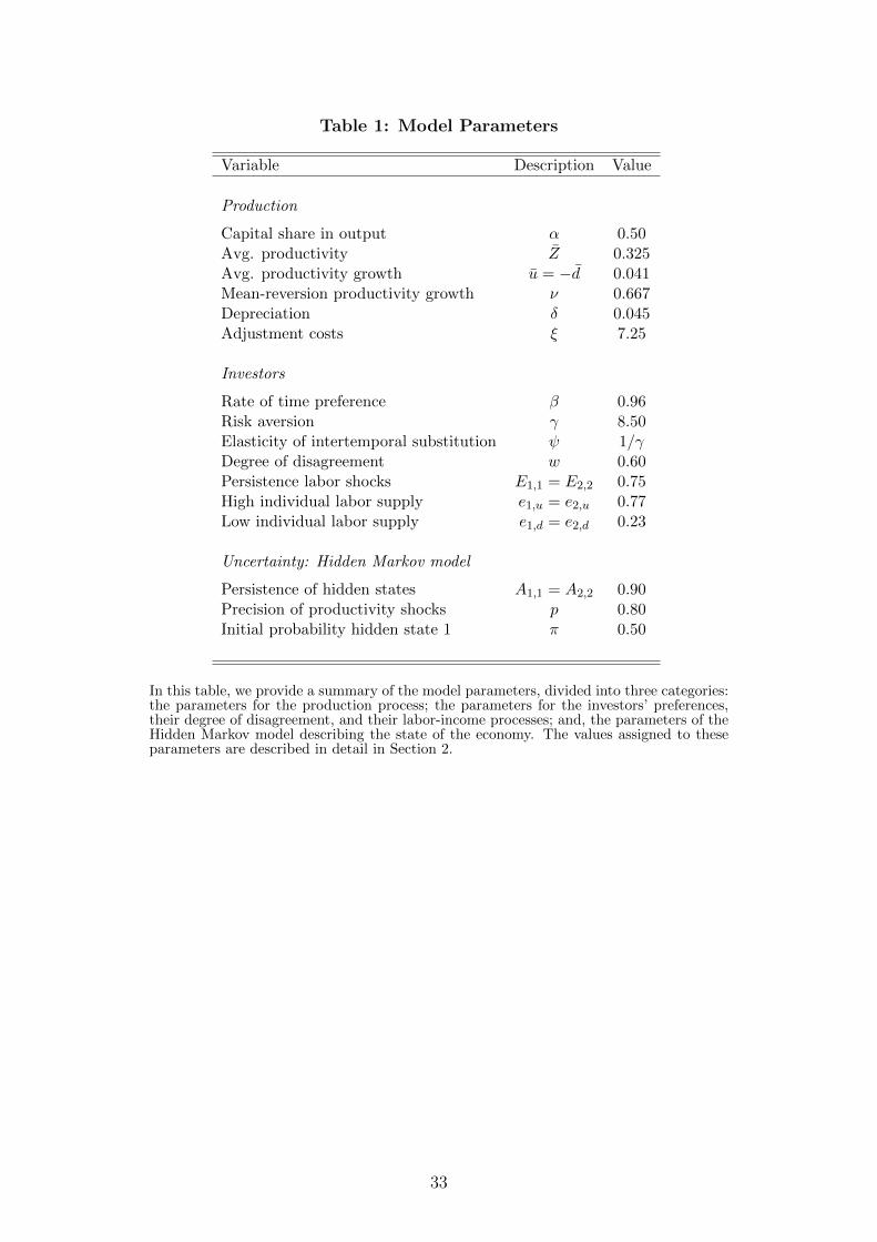
Table 1: Model Parameters

Variable Description Value

Production

Capital share in output α 0.50Avg. productivity Z 0.325Avg. productivity growth u = −d 0.041Mean-reversion productivity growth ν 0.667Depreciation δ 0.045Adjustment costs ξ 7.25

Investors

Rate of time preference β 0.96Risk aversion γ 8.50Elasticity of intertemporal substitution ψ 1/γDegree of disagreement w 0.60Persistence labor shocks E1,1 = E2,2 0.75High individual labor supply e1,u = e2,u 0.77Low individual labor supply e1,d = e2,d 0.23

Uncertainty: Hidden Markov model

Persistence of hidden states A1,1 = A2,2 0.90Precision of productivity shocks p 0.80Initial probability hidden state 1 π 0.50

In this table, we provide a summary of the model parameters, divided into three categories:the parameters for the production process; the parameters for the investors’ preferences,their degree of disagreement, and their labor-income processes; and, the parameters of theHidden Markov model describing the state of the economy. The values assigned to theseparameters are described in detail in Section 2.

33

Table 2: Financial and Business Cycle Statistics

Disagreement

Description Variable U.S. Data Yes No

Financial markets

Interest rate rf 1.94% 2.31% 3.36%Interest rate volatility σ(rf ) 5.44% 4.89% 2.30%Levered equity premium E[Rep] 6.17% 6.97% 4.50%Levered stock return volatility σ(R) 19.30% 17.19% 13.29%Log price-dividend ratio log(S/D) 3.10 3.06 3.11Volatility price-dividend ratio σ(log(S/D)) 26.30% 19.60% 13.40%

Real economy

Output growth E[Y ] 1.60% 0.91% 1.08%Output growth volatility σ(Y ) 3.78% 3.93% 3.94%Norm. investment growth volatility σ(I)/σ(Y ) 2.39 2.04 1.46Norm. consumption growth volatility σ(C)/σ(Y ) 0.40 0.71 0.87

Turnover

Bond market - 0.203 0.013Stock market - 0.139 0.027

Welfare (certainty consumption)

Econometrician’s measure - 0.1238 0.1289Subjective measure - 0.1312 0.1288

In this table, we provide a summary of various moments in the data and in the calibratedmodel for financial markets and macroeconomic variables. The calibration of the model is

described in Section 4.1, and the moments for the data are taken from Guvenen (2009). Notethat normalized investment-growth volatility is the ratio of investment growth volatilityto output volatility and normalized consumption volatility is the ratio of consumptionvolatility to output volatility. All model moments are computed using data from the last 50years of the 25, 000 simulations when the economy has reached its steady-state distribution.

34

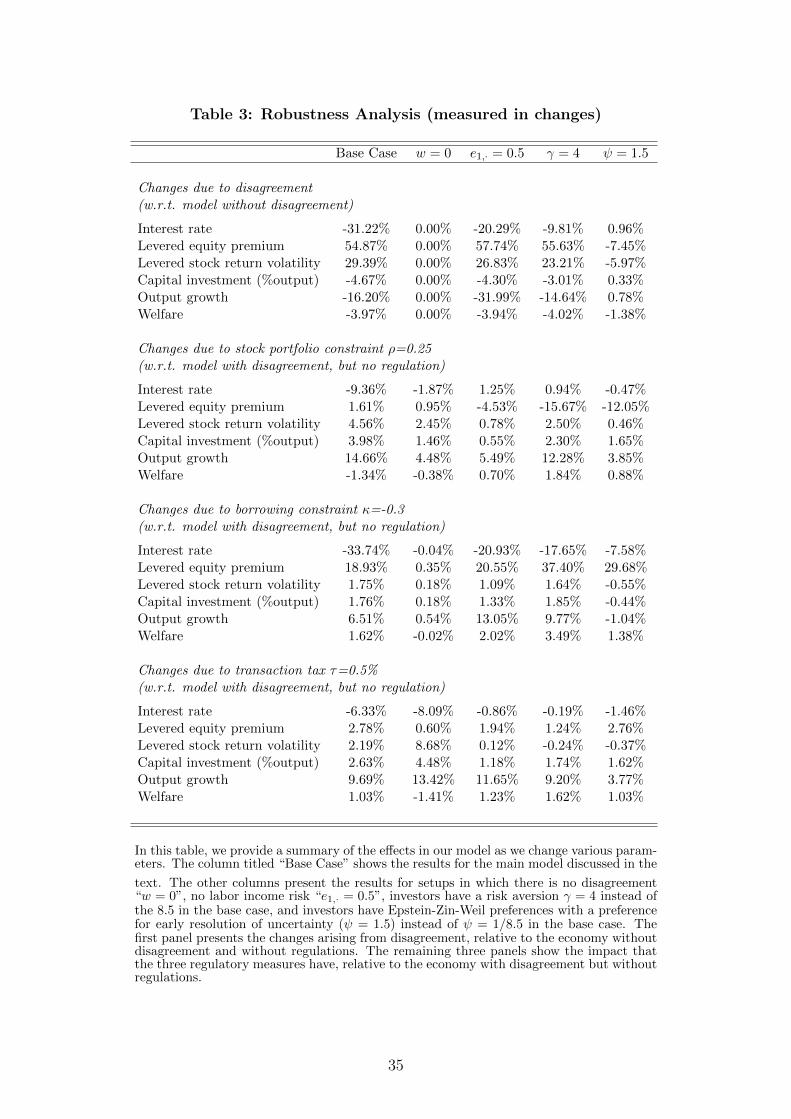
Table 3: Robustness Analysis (measured in changes)

Base Case w = 0 e1,· = 0.5 γ = 4 ψ = 1.5

Changes due to disagreement(w.r.t. model without disagreement)

Interest rate -31.22% 0.00% -20.29% -9.81% 0.96%Levered equity premium 54.87% 0.00% 57.74% 55.63% -7.45%Levered stock return volatility 29.39% 0.00% 26.83% 23.21% -5.97%Capital investment (%output) -4.67% 0.00% -4.30% -3.01% 0.33%Output growth -16.20% 0.00% -31.99% -14.64% 0.78%Welfare -3.97% 0.00% -3.94% -4.02% -1.38%

Changes due to stock portfolio constraint ρ=0.25(w.r.t. model with disagreement, but no regulation)

Interest rate -9.36% -1.87% 1.25% 0.94% -0.47%Levered equity premium 1.61% 0.95% -4.53% -15.67% -12.05%Levered stock return volatility 4.56% 2.45% 0.78% 2.50% 0.46%Capital investment (%output) 3.98% 1.46% 0.55% 2.30% 1.65%Output growth 14.66% 4.48% 5.49% 12.28% 3.85%Welfare -1.34% -0.38% 0.70% 1.84% 0.88%

Changes due to borrowing constraint κ=-0.3(w.r.t. model with disagreement, but no regulation)

Interest rate -33.74% -0.04% -20.93% -17.65% -7.58%Levered equity premium 18.93% 0.35% 20.55% 37.40% 29.68%Levered stock return volatility 1.75% 0.18% 1.09% 1.64% -0.55%Capital investment (%output) 1.76% 0.18% 1.33% 1.85% -0.44%Output growth 6.51% 0.54% 13.05% 9.77% -1.04%Welfare 1.62% -0.02% 2.02% 3.49% 1.38%

Changes due to transaction tax τ=0.5%(w.r.t. model with disagreement, but no regulation)

Interest rate -6.33% -8.09% -0.86% -0.19% -1.46%Levered equity premium 2.78% 0.60% 1.94% 1.24% 2.76%Levered stock return volatility 2.19% 8.68% 0.12% -0.24% -0.37%Capital investment (%output) 2.63% 4.48% 1.18% 1.74% 1.62%Output growth 9.69% 13.42% 11.65% 9.20% 3.77%Welfare 1.03% -1.41% 1.23% 1.62% 1.03%

In this table, we provide a summary of the effects in our model as we change various param-eters. The column titled “Base Case” shows the results for the main model discussed in the

text. The other columns present the results for setups in which there is no disagreement“w = 0”, no labor income risk “e1,· = 0.5”, investors have a risk aversion γ = 4 instead ofthe 8.5 in the base case, and investors have Epstein-Zin-Weil preferences with a preferencefor early resolution of uncertainty (ψ = 1.5) instead of ψ = 1/8.5 in the base case. Thefirst panel presents the changes arising from disagreement, relative to the economy withoutdisagreement and without regulations. The remaining three panels show the impact thatthe three regulatory measures have, relative to the economy with disagreement but withoutregulations.

35

Figure 1: Histograms

Stock Holdings Investor 10 0.5 1

0

0.5

1

1.5

Stock Holdings Investor 10 0.5 1

0

0.5

1

1.5

Borrowing Investor 1 (%output)-1.5 -1 -0.5 0 0.5 1 1.5

0

0.5

1

1.5

2

2.5

3

Borrowing Investor 1 (%output)-1.5 -1 -0.5 0 0.5 1 1.5

0

0.5

1

1.5

2

2.5

3

Stock Turnover0.1 0.2 0.3 0.4 0.5 0.6

0

5

10

15

20

25

30

Stock Turnover0.1 0.2 0.3 0.4 0.5 0.6

0

5

10

15

20

25

30

With Disagreement Without Disagreement

This figure depicts the simulated distribution of three variables: the first row shows the stock holdingsof Investor 1, the second row shows the first investor’s borrowing as a share of total output, andthe third row shows stock turnover. The figures on the left-hand side column are for the economy“with disagreement” in which investors disagree about the state of the economy, and the figures inthe right-hand side column are for the economy “without disagreement.” The histogram shows thequantities at the end of the horizon of a 200 year simulation with 25,000 paths. The histograms arenormalized to integrate to one.

36

Figure 2: Simulated path of the economy

180 182 184 186 188 190 192 194

Sto

ck H

oldi

ngs

-0.2

0

0.2

0.4

0.6

180 182 184 186 188 190 192 194

Bon

d H

oldi

ngs

-2

0

2

180 182 184 186 188 190 192 194

Sto

ck H

oldi

ngs

-0.2

0

0.2

0.4

0.6

180 182 184 186 188 190 192 194

Bon

d H

oldi

ngs

-2

0

2

180 182 184 186 188 190 192 194

Sto

ck H

oldi

ngs

-0.2

0

0.2

0.4

0.6

180 182 184 186 188 190 192 194

Bon

d H

oldi

ngs

-2

0

2

180 182 184 186 188 190 192 194

Sto

ck H

oldi

ngs

-0.2

0

0.2

0.4

0.6

180 182 184 186 188 190 192 194

Bon

d H

oldi

ngs

-2

0

2

Without disagreement With disagreement With disagreement and regulation

Basic Model

Stock portfolio constraint ; = 0.25

Borrowing constraint 5 = 0.1

Transaction tax = = 1%

The figure shows a simulated path of the economy for years 180 to 194. The first row depicts theevolution of the first investor’s stock holdings (number of shares) and bond holdings (% output) inthe basic (unregulated) economy in the absence (solid line) as well as in the presence of disagreement(dashed line); the second to fourth rows show the evolution of the holdings in the presence of differentregulatory measures (thick dotted line) and, for comparison, also their evolution in the absence ofregulation.

37

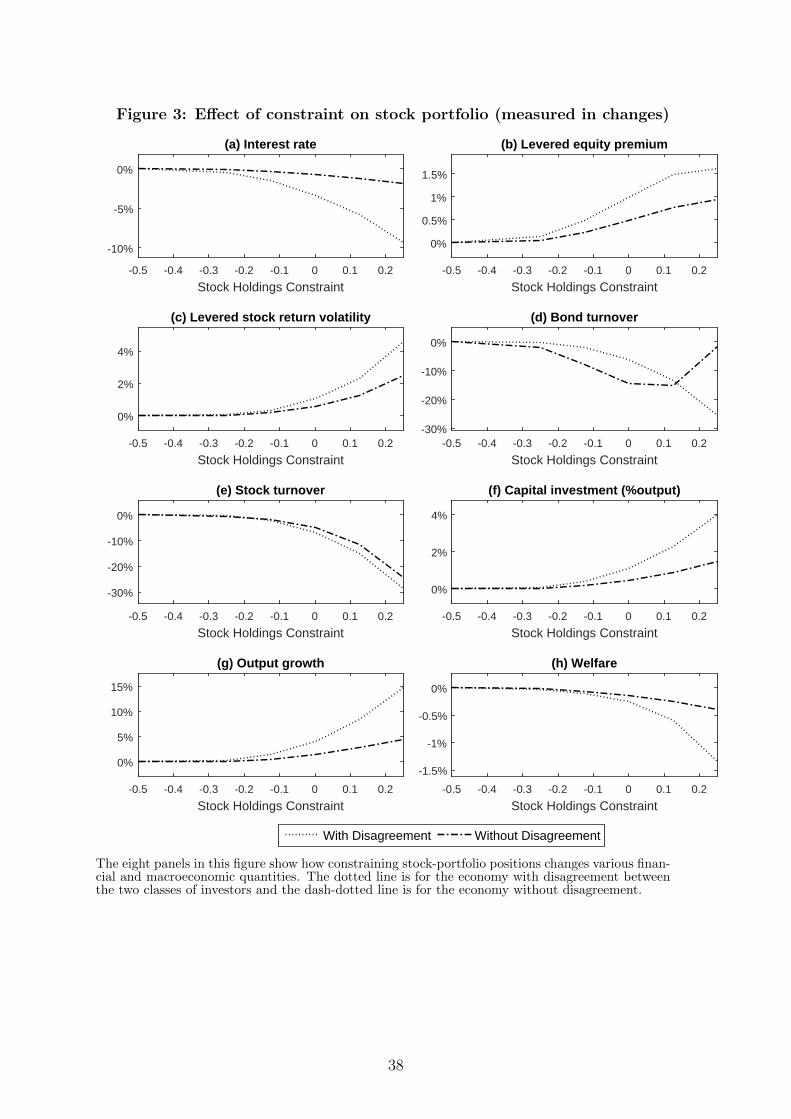
Figure 3: Effect of constraint on stock portfolio (measured in changes)

Stock Holdings Constraint-0.5 -0.4 -0.3 -0.2 -0.1 0 0.1 0.2

-10%

-5%

0%

(a) Interest rate

Stock Holdings Constraint-0.5 -0.4 -0.3 -0.2 -0.1 0 0.1 0.2

0%

0.5%

1%

1.5%

(b) Levered equity premium

Stock Holdings Constraint-0.5 -0.4 -0.3 -0.2 -0.1 0 0.1 0.2

0%

2%

4%

(c) Levered stock return volatility

Stock Holdings Constraint-0.5 -0.4 -0.3 -0.2 -0.1 0 0.1 0.2

-30%

-20%

-10%

0%

(d) Bond turnover

Stock Holdings Constraint-0.5 -0.4 -0.3 -0.2 -0.1 0 0.1 0.2

-30%

-20%

-10%

0%

(e) Stock turnover

Stock Holdings Constraint-0.5 -0.4 -0.3 -0.2 -0.1 0 0.1 0.2

0%

2%

4%

(f) Capital investment (%output)

Stock Holdings Constraint-0.5 -0.4 -0.3 -0.2 -0.1 0 0.1 0.2

0%

5%

10%

15%

(g) Output growth

Stock Holdings Constraint-0.5 -0.4 -0.3 -0.2 -0.1 0 0.1 0.2

-1.5%

-1%

-0.5%

0%

(h) Welfare

With Disagreement Without Disagreement

The eight panels in this figure show how constraining stock-portfolio positions changes various finan-cial and macroeconomic quantities. The dotted line is for the economy with disagreement betweenthe two classes of investors and the dash-dotted line is for the economy without disagreement.

38

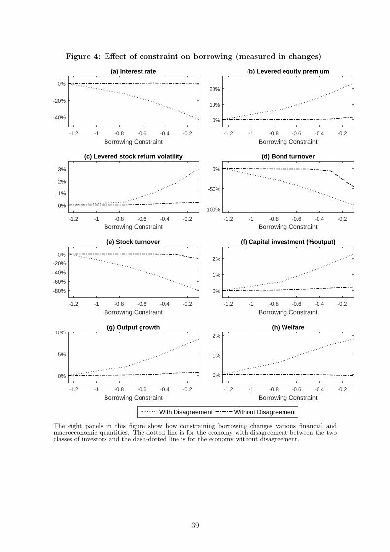
Figure 4: Effect of constraint on borrowing (measured in changes)

Borrowing Constraint-1.2 -1 -0.8 -0.6 -0.4 -0.2

-40%

-20%

0%

(a) Interest rate

Borrowing Constraint-1.2 -1 -0.8 -0.6 -0.4 -0.2

0%

10%

20%

(b) Levered equity premium

Borrowing Constraint-1.2 -1 -0.8 -0.6 -0.4 -0.2

0%

1%

2%

3%

(c) Levered stock return volatility

Borrowing Constraint-1.2 -1 -0.8 -0.6 -0.4 -0.2

-100%

-50%

0%

(d) Bond turnover

Borrowing Constraint-1.2 -1 -0.8 -0.6 -0.4 -0.2

-80%

-60%

-40%

-20%

0%

(e) Stock turnover

Borrowing Constraint-1.2 -1 -0.8 -0.6 -0.4 -0.2

0%

1%

2%

(f) Capital investment (%output)

Borrowing Constraint-1.2 -1 -0.8 -0.6 -0.4 -0.2

0%

5%

10%(g) Output growth

Borrowing Constraint-1.2 -1 -0.8 -0.6 -0.4 -0.2

0%

1%

2%

(h) Welfare

With Disagreement Without Disagreement

The eight panels in this figure show how constraining borrowing changes various financial andmacroeconomic quantities. The dotted line is for the economy with disagreement between the twoclasses of investors and the dash-dotted line is for the economy without disagreement.

39

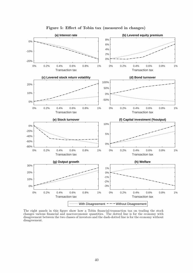
Figure 5: Effect of Tobin tax (measured in changes)

Transaction tax 0% 0.2% 0.4% 0.6% 0.8% 1%

-20%

-10%

0%

(a) Interest rate

Transaction tax 0% 0.2% 0.4% 0.6% 0.8% 1%

0%

2%

4%

6%

8%

(b) Levered equity premium

Transaction tax 0% 0.2% 0.4% 0.6% 0.8% 1%

0%

10%

20%

(c) Levered stock return volatility

Transaction tax 0% 0.2% 0.4% 0.6% 0.8% 1%

-50%

0%

50%

100%

(d) Bond turnover

Transaction tax 0% 0.2% 0.4% 0.6% 0.8% 1%

-80%

-60%

-40%

-20%

0%

(e) Stock turnover

Transaction tax 0% 0.2% 0.4% 0.6% 0.8% 1%

0%

5%

10%

(f) Capital investment (%output)

Transaction tax 0% 0.2% 0.4% 0.6% 0.8% 1%

0%

10%

20%

30%(g) Output growth

Transaction tax 0% 0.2% 0.4% 0.6% 0.8% 1%

-3%

-2%

-1%

0%

1%

(h) Welfare

With Disagreement Without Disagreement

The eight panels in this figure show how a Tobin financial-transaction tax on trading the stockchanges various financial and macroeconomic quantities. The dotted line is for the economy withdisagreement between the two classes of investors and the dash-dotted line is for the economy withoutdisagreement.

40

Online Appendix

In this appendix, we first provide the derivations for the characterization of equilib-

rium. Next, we present the steady-state distributions of productivity as well as the first

investor’s consumption share. Finally, the appendix contains the figures presented in the

paper, but with the relevant quantities shown in levels instead of changes.

A Characterization of equilibrium

We first discuss the firm’s optimization problem and then the investors’ optimization

problem without and with financial regulation. At the end of the section, we describe

the numerical algorithm used to solve the model.

A.1 Derivations of Optimality Conditions

A.1.1 Optimality Conditions: Representative Firm

The objective of the firm is to choose investment It and labor Lt to maximize its value,

given in equation (3), subject to the law-of-motion of capital, as outlined in equation (2).

Computing the first-order condition with respect to labor Lt results in

∂Pt∂Lt

=∂Yt∂Lt−Wt = (1− α)ZtKtL

−αt −Wt = 0 (A1)

Using the result that, on aggregate, investors always provide one unit of labor, we get

Wt = (1− α)ZtKt = (1− α)Yt, (A2)

so that dividends of the firm can be rewritten as: Dt = αYt − It. Plugging this into the

optimization problem of the firm and maximizing with respect to It gives:

∂Pt∂It

= −1 +J∑j=1

qt+1,j∂Pt+1,j

∂Kt+1,j

(1− ξ It

Kt

)= 0, (A3)

A1

Invoking the envelope condition, we get:

∂Pt∂Kt

=

(αZt −

∂It∂Kt

)+

(J∑j=1

qt+1,j∂Pt+1,j

∂Kt+1,j

)∂Kt+1

∂Kt

(A4)

= αZt −∂It∂Kt

+1

1− ξ ItKt

∂Kt+1

∂Kt

(A5)

= αZt −∂It∂Kt

+1

1− ξ ItKt

((1− δ) +

∂It∂Kt

− ξ

2

(ItKt

)2

− ξ ItKt

(∂It∂Kt

− ItKt

))(A6)

= αZt +1− δ + ξ It

Kt

1− ξ ItKt

, (A7)

where we used equation (A3) in the second step to substitute the expectation. Plugging

(A7), for time t+ 1, into (A3), we get equation (14) in the paper:

(1− ξ It

Kt

)×

J∑j=1

qt+1,j

(αZt+1,j +

1− δ + ξ2

(It+1,j

Kt+1

)2

1− ξ It+1,j

Kt+1

)= 1. (A8)

A.1.2 Optimality Conditions: Investors in Absence of Regulatory Measures

The objective of each investor i is to maximize lifetime utility given in (4), subject to the

flow budget equation (5), by choosing consumption, ci,t, and the portfolio position θ{B,S}i,t

in each of the two financial assets. The Lagrangian associated with this problem is given

by:

Li,t = supci,t,θ

Si,t,θ

Bi,t

infRBCi,t

[(1− β) c

1− 1ψ

i,t + βEit[V 1−γi,t+1

] 1φ

] φ1−γ

+RBCi,t

[ei,tWt + θBi,t−1 + θSi,t−1

(St +Dt

)− ci,t − θSi,tSt − θBi,tBt

], (A9)

where RBCi,t denotes the Lagrange multiplier associated with the budget equation.

A2

The first-order condition of (A9) with respect to consumption ci,t is given by:

∂Li,t∂ci,t

=1

1− 1ψ

{(1− β) c

1− 1ψ

i,t + βEit[V 1−γi,t+1

] 1− 1ψ

1−γ

} 1

1− 1ψ

−1

(1− β)

(1− 1

ψ

)c

1− 1ψ−1

i,t −RBCi,t

= (1− β) c− 1ψ

i,t

{(1− β) c1− 1

ψ

i,t + βEit[V 1−γi,t+1

] 1− 1ψ

1−γ

} 1

1− 1ψ

1ψ

−RBCi,t

= (1− β) c− 1ψ

i,t V1ψ

i,t −RBCi,t ≡ 0. (A10)

Second, the first-order condition of (A9) with respect to the Lagrange multiplier RBCi,t :

∂Li,t∂RBC

i,t

=[ei,tWt + θBi,t−1 + θSi,t−1

(St +Dt

)− θBt Bt − θSi,tSt − ci,t

]≡ 0. (A11)

Third, the first-order condition of (A9) with respect to the bond holdings θBi,t:

∂Li,t∂θBi,t

=1

1− 1ψ

{(1− β) c

1− 1ψ

i,t + βEit[V 1−γi,t+1

] 1− 1ψ

1−γ

} 1

1− 1ψ

−1

×

β1− 1

ψ

1− γEit[V 1−γi,t+1

] 1− 1ψ

1−γ −1(1− γ)Eit

[V −γi,t+1

∂Vi,t+1

∂θBi,t

]−RBC

i,t Bt

= βV1ψ

i,tEit[V 1−γi,t+1

] 1− 1ψ

1−γ −1 Eit

[V −γi,t+1

∂Vi,t+1

∂θBi,t

]−RBC

i,t Bt ≡ 0, (A12)

and the first-order condition with respect to the stock holdings θSi,t:

∂Li,t∂θSi,t

=1

1− 1ψ

{(1− β) c

1− 1ψ

i,t + βEit[V 1−γi,t+1

] 1− 1ψ

1−γ

} 1

1− 1ψ

−1

×

β1− 1

ψ

1− γEit[V 1−γi,t+1

] 1− 1ψ

1−γ −1(1− γ)Eit

[V −γi,t+1

∂Vi,t+1

∂θSi,t

]−RBC

i,t St

= βV1ψ

i,tEit[V 1−γi,t+1

] 1− 1ψ

1−γ −1 Eit

[V −γi,t+1

∂Vi,t+1

∂θSi,t

]−RBC

i,t St ≡ 0. (A13)

Invoking the envelope theorem, we can replace the derivative of the value function

with the partial derivative of the Lagrangian, assuming that the decision variables are

A3

at their optimum, and hence, the first-order conditions with respect to decision variables

are satisfied. Differentiating the original Lagrangian (A9) with respect to past holdings,

we get:

∂Vi,t

∂θBi,t−1

=∂Li,t∂θBi,t−1

= RBCi,t , (A14)

∂Vi,t

∂θSi,t−1

=∂Li,t∂θSi,t−1

= RBCi,t ×

(Si,t +Dt

). (A15)

To summarize, the first-order conditions that characterize the investors’ optimization

problem are given by:

ci,t + θBi,tBt + θSi,t St = θBi,t−1 + θSi,t−1 (Dt + St) + ei,tWt, (A16)

Bt = Eit[Mi,t+1

Mi,t

], (A17)

St = Eit[Mi,t+1

Mi,t

× (St+1 +Dt+1)

], (A18)

whereMi,t+1

Mi,tdenotes the investors’ pricing kernel for Epstein-Zin-Weil utility:

Mi,t+1

Mi,t

= β

(V 1−γi,t+1

Eit[V 1−γi,t+1

])1ψ

−γ1−γ (

ci,t+1

ci,t

)− 1ψ

. (A19)

Equation (A16) is the budget constraint that the consumption and portfolio policies must

satisfy. Intuitively, equations (A17) and (A18) equate the benefit from holding an asset

to the benefit from selling it.

A.1.3 Optimality Conditions: Investors in Presence of Regulatory Measures

We now derive the optimality conditions for the setups with a constraint on stock holdings,

a borrowing constraint, and the Tobin tax on stock transactions.

Portfolio Constraint

The Lagrangian associated with lifetime utility (4), the budget constraint (5), and the

A4

portfolio constraint (11) is given by:

Li,t = supci,t,θ

Si,t

infRBCi,t ,R

Si,t

[(1− β) c

1− 1ψ

i,t + βEit[V 1−γi,t+1

] 1φ

] φ1−γ

+RBCi,t

[ei,tWt + θBi,t−1 + θSi,t−1

(St +Dt

)− ci,t − θSi,tSt − θBi,tBt

]+RBC

i,t RSi,tSt × (θSi,t − ρ), (A20)

where RBCi,t and RBC

i,t RSi,tSt denote the Lagrange multipliers associated with the budget

constraint and the portfolio constraint, respectively.

The derivations are similar to the derivations for the economy without regulation

discussed above. Only the first-order condition with respect to the stock holdings changes

to:

∂Li,t∂θSi,t

= βV1ψ

i,tEit[V 1−γi,t+1

] 1− 1ψ

1−γ −1 Eit

[V −γi,t+1

∂Vi,t+1

∂θSi,t

]−RBC

i,t St +RBCi,t R

Si,tSt ≡ 0, (A21)

such that the kernel condition of the stock becomes

Si,t =1

1−RSi,t

× Eit

[Mi,t+1

Mi,t

(Si,t+1 +Dt+1

)]. (A22)

In addition, we get the following complimentary slackness and inequality conditions:

RSi,t × (θSi,t − ρ) = 0; RS

i,t ≥ 0; θSi,t ≥ ρ. (A23)

Borrowing Constraint

The Lagrangian associated with lifetime utility (4), the budget constraint (5), and the

borrowing constraint (12), is:

Li,t = supci,t,θ

Si,t,θ

Bi,t

infRBCi,t ,R

Bi,t

[(1− β) c

1− 1ψ

i,t + βEit[V 1−γi,t+1

] 1φ

] φ1−γ

+RBCi,t

[ei,tWt + θBi,t−1 + θSi,t−1

(St +Dt

)− ci,t − θSi,tSt − θBi,tBt

]+RBC

i,t RBi,t × (θBi,tBt − κYt), (A24)

A5

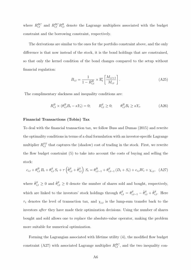
where RBCi,t and RBC

i,t RBi,t denote the Lagrange multipliers associated with the budget

constraint and the borrowing constraint, respectively.

The derivations are similar to the ones for the portfolio constraint above, and the only

difference is that now instead of the stock, it is the bond holdings that are constrained,

so that only the kernel condition of the bond changes compared to the setup without

financial regulation:

Bi,t =1

1−RBi,t

× Eit[Mi,t+1

Mi,t

]. (A25)

The complimentary slackness and inequality conditions are:

RBi,t × (θBi,tBt − κYt) = 0; RS

i,t ≥ 0; θBi,tBt ≥ κYt. (A26)

Financial Transactions (Tobin) Tax

To deal with the financial transaction tax, we follow Buss and Dumas (2015) and rewrite

the optimality conditions in terms of a dual formulation with an investor-specific Lagrange

multiplier RTTi,t that captures the (shadow) cost of trading in the stock. First, we rewrite

the flow budget constraint (5) to take into account the costs of buying and selling the

stock:

ci,t + θBi,tBt + θSi,t St + τ(θSi,t + θSi,t

)St = θBi,t−1 + θSi,t−1 (Dt + St) + ei,tWt + χi,t, (A27)

where θSi,t ≥ 0 and θSi,t ≥ 0 denote the number of shares sold and bought, respectively,

which are linked to the investors’ stock holdings through θSi,t = θSi,t−1 − θSi,t + θSi,t. Here

τ t denotes the level of transaction tax, and χi,t is the lump-sum transfer back to the

investors after they have made their optimization decisions. Using the number of shares

bought and sold allows one to replace the absolute-value operator, making the problem

more suitable for numerical optimization.

Forming the Lagrangian associated with lifetime utility (4), the modified flow budget

constraint (A27) with associated Lagrange multiplier RBCi,t , and the two inequality con-

A6

ditions (θSi,t ≥ 0 and θSi,t ≥ 0) with multipliers µ1,i,t and µ2,i,t for the selling and buying

decision, we get:

Li,t = supci,t,θ

Bi,t,θ

Si,t,θ

Si,t

infRBCi,t ,µ1,i,t,µ2,i,t

[(1− β) c

1− 1ψ

i,t + βEit[V 1−γi,t+1

] 1φ

] φ1−γ

(A28)

+RBCi,t

[ei,tWt + ξi,tθ

Bi,t−1 + θSi,t−1

(St +Dt

)− ci,t − θSi,t St + τ

(θSi,t + θSi,t

)St − θBi,tBt

]+ µ1,i,t × θSi,t + µ2,i,t × θSi,t,

with θSi,t = θSi,t−1 − θSi,t + θSi,t.

Differentiating the resulting Lagrangian with respect to current consumption ci,t, with

respect to bond holdings, and with respect to the new variables θSi,t and θSi,t for the stock,

we obtain the following first-order conditions:

(1− β) c− 1ψ

i,t V1ψ

i,t = RBCi,t (A29)

βV1ψ

i,tEit[V 1−γi,t+1

] 1− 1ψ

1−γ −1 Eit

[V −γi,t+1

∂Vi,t+1

∂θSi,t

]= −RBC

i,t (1 + τ)Si,t + µ1,i,t (A30)

βV1ψ

i,tEit[V 1−γi,t+1

] 1− 1ψ

1−γ −1 Eit

[V −γi,t+1

∂Vi,t+1

∂θSi,t

]= RBC

i,t (1− τ)Si,t + µ2,i,t (A31)

βV1ψ

i,tEit[V 1−γi,t+1

] 1− 1ψ

1−γ −1 Eit

[V −γi,t+1

∂Vi,t+1

∂θBi,t

]= RBC

i,t Bt (A32)

ci,t + θBi,tBt + θSi,t St + τ(θSi,t + θSi,t

)St = θBi,t−1 + θSi,t−1 (Dt + St) + ei,tWt + χi,t, (A33)

µ1,i,tθSi,t = 0, µ2,i,tθ

Si,t = 0, µ{1,2},i,t ≥ 0, θSi,t ≥ 0, θSi,t ≥ 0. (A34)

Note that equations (A30) and (A31) imply

−RBCi,t (1 + τ)Si,t + µ1,i,t = RBC

i,t (1− τ)Si,t + µ2,i,t, (A35)

so that we can replace the two multipliers µ{1,2},k,t with one multiplier RTTi,t , defined as:

RBCi,t R

TTi,t Si,t

def= −RBC

i,t (1 + τ)Si,t + µ1,i,t = RBCi,t (1− τ)Si,t + µ2,i,t. (A36)

A7

From (A36), it follows that

µ1,i,t = RBCi,t Si,t(R

TTi,t + 1 + τ), (A37)

µ2,i,t = RBCi,t Si,t(R

TTi,t − 1 + τ), (A38)

so that we can rewrite the slackness conditions respectively:

(RTTi,t + 1 + τ)θSi,t = 0, (A39)

(RTTi,t − 1 + τ)θSi,t = 0. (A40)

Using the slackness conditions, we can rewrite the flow budget equation as follows:

ei,tWt + χi,t + θSk,t−1Dt − ci,t + θBk,t−1 − θBk,tBi,t − (θSk,t − θSk,t−1)Si,tRTTi,t = 0. (A41)

Now, apply the Envelope Theorem to get rid of the value function in the first-order

conditions:

∂Vk,t+1

∂θBk,t= RBC

i,t+1Bk,t+1, (A42)

∂Vk,t+1

∂θSk,t= RBC

i,t+1(RTTi,t+1St+1 +Dt+1), (A43)

and finally get the following system:

St =1

RTTi,t

× Eit[Mi,t+1

Mi,t

(RTTi,t+1St+1 +Dt+1

)], (A44)

Bt = Eit[Mi,t+1

Mi,t

], (A45)

ci,t +(θSi,t − θSi,t−1

)Si,tR

TTi,t + θBk,tBi,t = θSk,t−1Dt + θBk,t−1 + χi,t + ei,tWt, (A46)

(RTTi,t + 1 + τ)θSi,t = 0, (RTT

i,t − 1 + τ)θSi,t = 0, (A47)

1− τ ≤ RTTi,t ≤ 1 + τ ; θSi,t ≥ 0; θSi,t ≥ 0. (A48)

A8

A.2 Equilibrium: Numerical Solution Method

The numerical method we use is not based on an approximation of any sort;20 it is exact

(except for local interpolation and, of course, numerical truncation error), which is a

distinct advantage considering the non linearities involved.

We wish to obtain the equilibrium in a numerical form by backward-induction. For

reasons explained in Dumas and Lyasoff (2012), the system of first-order conditions writ-

ten in the previous appendixes cannot be solved by backward induction. However, it

is possible to solve the equations by backward induction if one changes the sequence in

which the equations are solved, performing a re-grouping of equations in such a way that,

at a node of time t, one solves the equations yielding not consumption at time t and the

portfolio chosen at time t but, instead, consumption at the various successor nodes at

time t+ 1 and the portfolio at time t.

In this case, the first investor’s share of output c1,tYt

serves as an endogeneous state

variable. The capital stock Kt is an endogenous state variable as well but, under our

assumptions, a scale-invariance property holds so that it is only a scale variable, which

can be factored out of all the equations.

In the same way, that is, on a grid, we treat a variable, which is, in fact, exogenous and

which is imbedded in the conditional expected value operators Ei,t. Beliefs differ; hence

the subscript i on these operators. The way in which beliefs differ has been explained

in Section 2. Recall that we consider two hidden states and four observable states of a

Markov chain. Investors have immutable beliefs about the transition probabilities from

the two time-t hidden states to the two time-t+1 hidden states and, from there, to the four

time-t+1 observable states. But each of the two investors has to estimate the probability

of being at time t in one of the two hidden states. These estimated probabilities change

20Approximation methods commonly used are: Taylor series (the “perturbation” method) and linearcombinations of polynomials (the “projection” method).

A9

over time in response to the observations made in the past. By means of simulations of

the hidden Markov chain (the workings of which are exogenous to our model), we identify

the full, discrete list of pairs of these estimated probabilities that can occur at any time

and we place these on a grid.

In case of financial regulation, the complementary slackness conditions cause the sys-

tem to be ill-defined. As in Buss and Dumas (2015), we replace them with the following:

(1 + τ −Ri,t)θi,t = ε, (A49)

(−1 + τ +Ri,t)θi,t = ε, (A50)

and, as we approach the final solution, we let ε approach zero. That is called the “Interior-

Point Algorithm” (see Armand, Benoist, and Orban (2008)).

Moreover, in the case of the Tobin tax, the ratio of the investors’ shadow pricesRTT1,t

RTT2,t

is needed as another endogenous state variable.

B Steady state distributions

As discussed in the paper, our model of productivity growth implies a steady-state distri-

bution for productivity, as the growth rate is mean-reverting. Figure A1, first row, shows

the dynamics of the steady-state distribution of productivity over time, based on the pa-

rameters used in the paper. It also shows the standard deviation of productivity across

paths which indicates that the distribution quickly (after about 25 years) approaches it

steady state.

The second row of Figure A1 depicts the steady-state distribution of the first investor’s

consumption share which is nicely centered around 0.5 as both investors are perfectly

symmetric. It also shows the dynamics of the standard deviation of the consumption

share across paths over time, indicating that the distribution converges to its steady

state after about 150 years.

A10

Figure A1: Steady-state distributions

0.26 0.28 0.3 0.32 0.34 0.36 0.38 0.40

100

200

300

400

500

600

700Productivity

Time0 50 100 150 200

0

0.005

0.01

0.015

0.02

0.025

0.03

0.035Standard Deviation Productivity

0 0.2 0.4 0.6 0.8 10

200

400

600

800

1000

1200

1400Consumption Share Investor 1

Time0 50 100 150 200

0.01

0.02

0.03

0.04

0.05

0.06

0.07

0.08

0.09

0.1Standard Deviation Consumption Share Investor 1

The figure shows the steady-state distributions for productivity and the first investor’sconsumption share (left side), together with the dynamics of the standard deviation of thevariable across paths over time (right side).

A11

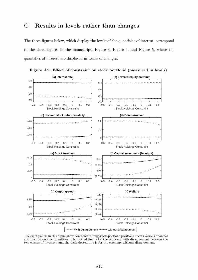
C Results in levels rather than changes

The three figures below, which display the levels of the quantities of interest, correspond

to the three figures in the manuscript, Figure 3, Figure 4, and Figure 5, where the

quantities of interest are displayed in terms of changes.

Figure A2: Effect of constraint on stock portfolio (measured in levels)

Stock Holdings Constraint-0.5 -0.4 -0.3 -0.2 -0.1 0 0.1 0.2

2%

3%

2%

3%

(a) Interest rate

Stock Holdings Constraint-0.5 -0.4 -0.3 -0.2 -0.1 0 0.1 0.2

4%

6%

4%

6%

(b) Levered equity premium

Stock Holdings Constraint-0.5 -0.4 -0.3 -0.2 -0.1 0 0.1 0.2

14%

16%

18%

(c) Levered stock return volatility

Stock Holdings Constraint-0.5 -0.4 -0.3 -0.2 -0.1 0 0.1 0.2

0

0.1

0.2

(d) Bond turnover

Stock Holdings Constraint-0.5 -0.4 -0.3 -0.2 -0.1 0 0.1 0.20

0.05

0.1

0.15

(e) Stock turnover

Stock Holdings Constraint-0.5 -0.4 -0.3 -0.2 -0.1 0 0.1 0.2

22.5%

23%

23.5%

24%

(f) Capital investment (%output)

Stock Holdings Constraint-0.5 -0.4 -0.3 -0.2 -0.1 0 0.1 0.2

0.9%

1%

1.1%

(g) Output growth

Stock Holdings Constraint-0.5 -0.4 -0.3 -0.2 -0.1 0 0.1 0.2

0.122

0.124

0.126

0.128

0.13(h) Welfare

With Disagreement Without Disagreement

The eight panels in this figure show how constraining stock-portfolio positions affects various financialand macroeconomic quantities. The dotted line is for the economy with disagreement between thetwo classes of investors and the dash-dotted line is for the economy without disagreement.

A12

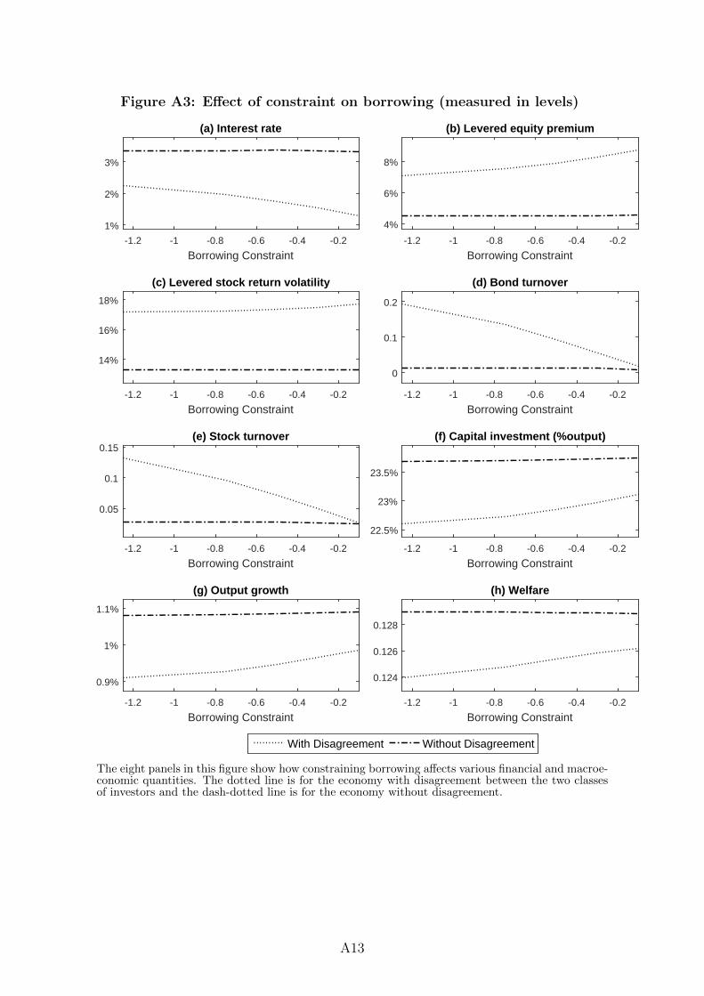
Figure A3: Effect of constraint on borrowing (measured in levels)

Borrowing Constraint-1.2 -1 -0.8 -0.6 -0.4 -0.2

1%

2%

3%

(a) Interest rate

Borrowing Constraint-1.2 -1 -0.8 -0.6 -0.4 -0.2

4%

6%

8%

(b) Levered equity premium

Borrowing Constraint-1.2 -1 -0.8 -0.6 -0.4 -0.2

14%

16%

18%

(c) Levered stock return volatility

Borrowing Constraint-1.2 -1 -0.8 -0.6 -0.4 -0.2

0

0.1

0.2

(d) Bond turnover

Borrowing Constraint-1.2 -1 -0.8 -0.6 -0.4 -0.2

0.05

0.1

0.15(e) Stock turnover

Borrowing Constraint-1.2 -1 -0.8 -0.6 -0.4 -0.2

22.5%

23%

23.5%

(f) Capital investment (%output)

Borrowing Constraint-1.2 -1 -0.8 -0.6 -0.4 -0.2

0.9%

1%

1.1%

(g) Output growth

Borrowing Constraint-1.2 -1 -0.8 -0.6 -0.4 -0.2

0.124

0.126

0.128

(h) Welfare

With Disagreement Without Disagreement

The eight panels in this figure show how constraining borrowing affects various financial and macroe-conomic quantities. The dotted line is for the economy with disagreement between the two classesof investors and the dash-dotted line is for the economy without disagreement.

A13

Figure A4: Effect of Tobin tax (measured in levels)

Transaction tax 0% 0.2% 0.4% 0.6% 0.8% 1%

2%

2.5%

3%

3.5%

(a) Interest rate

Transaction tax 0% 0.2% 0.4% 0.6% 0.8% 1%

4%

6%

8%(b) Levered equity premium

Transaction tax 0% 0.2% 0.4% 0.6% 0.8% 1%

14%

16%

18%

(c) Levered stock return volatility

Transaction tax 0% 0.2% 0.4% 0.6% 0.8% 1%

0

0.1

0.2

(d) Bond turnover

Transaction tax 0% 0.2% 0.4% 0.6% 0.8% 1%

0

0.05

0.1

0.15

(e) Stock turnover

Transaction tax 0% 0.2% 0.4% 0.6% 0.8% 1%

22%

24%

26%

(f) Capital investment (%output)

Transaction tax 0% 0.2% 0.4% 0.6% 0.8% 1%

1%

1.2%

1.4%

(g) Output growth

Transaction tax 0% 0.2% 0.4% 0.6% 0.8% 1%

0.124

0.126

0.128

(h) Welfare

With Disagreement Without Disagreement

The eight panels in this figure show how a Tobin financial-transaction tax on trading the stockaffects various financial and macroeconomic quantities. The dotted line is for the economy withdisagreement between the two classes of investors and the dash-dotted line is for the economywithout disagreement.

A14

SAFE | Ho

Recen

No. 123

No. 122

No. 121 No. 120 No. 119

No. 118

No. 117

No. 116 No. 115

No. 114

No. 113

No. 112

No. 111

No. 110 No. 109

ouse of Finan

nt Issues

Marie L

Dougla

Jochen

Elia Ber

Matthi

Michae

Michae

Paradis

Marcel

Charles

Andrea

Luigi G

Nicole Wu

Bettina

Shafik

Weiche

Alfons Xu

Dirk Kr

Tobias

nce | Goethe

s

Lalanne, Pau

as Cumming Werth

rdin, Matteo

as Heinz, H

el Brennan,

el Donadelliso, Max Ried

Bluhm

s Gottlieb

as Fagereng,uiso

Branger, Ch

a Brüggema

Hebous, Alfenrieder

J. Weichenr

ueger, Alexa

Tröger

University Fr

ul Seabright

g, Uwe Walz

o Sottocorno

einer Schum

Holger Kraft

, Antonio del

, Charles Go

hristian Schl

nn, Jinhyuk

fons J.

rieder, Fangy

ander Ludw

rankfurt | ww

t TPE

z, THa

ola I

macher S

ft Lt

AI

I(

O

ottlieb, AC

ag, Lue 'SD

k Yoo AI

O

ying AC

wig O

Rt

ww.safe-frank

The Old BoyProfessionaExecutive Jo

The DynamiHigh-Tech Vand Exit

nsurance A

Signaling Co

Leaning Agathe Face of A

A Quasi Reandustrial Pr

nterbank Fu(Persistent)

On the Distr

Asset MarkeChoice over

Nobody is PSurvival WhDifferent Ki

Aggregate ancreasing T

On Deficits a

Are Tax HavCrackdown

On the Opti

Regulatory Ithe Banking

kfurt.de | info

y Network: Tl Networks o

obs

ics of EntrepVentures: Ex

ctivities and

ooperation

ainst the WiAdversity

l-Time Leadroduction

unding as InLiquidity Sh

ributive Effe

et Participatthe Life-Cyc

Perfect': Assehen Heterognds of Filter

and DistribuTaxes on Top

and Symme

vens Good? Ion Secrecy

mal Provisio

Influence ong Union

o@safe.uni-f

The Impact oon Remune

preneurial Cxperience, Ed

d Systemic R

ind: Debt Fin

ding Indicato

nsurance Mehocks

ects of Inflat

tion and Porcle

et Pricing ageneous Invering Errors

utional Effecp Income Ea

etries in a Fis

Implication

on of Social

n Market Co

rankfurt.de

of ration in To

Careers in ducation,

Risk

nancing in

or for the EU

echanism fo

tion

rtfolio

nd Long-Ruestors Exhib

cts of arners

scal Capacit

s of the

Insurance

onditions in

 

op

U

or

n bit

ty