the initial impact of the crisis on emerging market …...market countries, we explore the role of...

263

HAMID FARUQEEInternational Monetary Fund

The Initial Impact of the Crisis onEmerging Market Countries

ABSTRACT To understand the diverse impact of the crisis across emergingmarket countries, we explore the role of two shocks—the collapse in trade andthe sharp decline in financial flows—in the transmission of the crisis from theadvanced economies. We first develop a simple open economy model, whichallows for imperfect capital mobility and potentially contractionary effects ofcurrency depreciation due to foreign debt exposure. We then look at the cross-country evidence. The data suggest a strong role for both trade and financialshocks. Perhaps surprisingly, the data give little econometric support for a cen-tral role of either reserves or exchange rate regimes. We end by presenting casestudies for Latvia, Russia, and Chile.

One of the striking characteristics of the financial crisis that originatedin the United States is how quickly and how broadly it spread to the

rest of the world. When the crisis intensified, first in the United States andthen in Europe, in the fall of 2008, emerging market countries thought theymight escape more or less unharmed. There was talk of decoupling. Thiswas not to be.

Figure 1 shows growth rates of GDP for a group of advanced economiesand a group of emerging market countries from the first quarter of 2006through 2009. The two series have moved largely in tandem. In the fourthquarter of 2008 and the first quarter of 2009, economic growth in theadvanced group averaged −7.2 percent and −8.3 percent, respectively (atannual rates). In the same two quarters, growth in the emerging marketcountries was −1.9 percent and −3.2 percent, respectively. As the figureshows, the better numbers for the emerging market countries reflect their

OLIVIER J. BLANCHARDInternational Monetary FundMassachusetts Institute of Technology

MITALI DASInternational Monetary Fund

12178-05a_Blanchard_rev1.qxd 8/11/10 12:16 PM Page 263

264 Brookings Papers on Economic Activity, Spring 2010

1. The countries and their abbreviations are as follows: Argentina (ARG), Brazil (BRA),Chile (CHL), China (CHN), Colombia (COL), Croatia (HRV), Czech Republic (CZE), Esto-nia (EST), Hungary (HUN), India (IND), Indonesia (IDN), Israel (ISR), Republic of Korea(KOR), Latvia (LVA), Lithuania (LTU), Malaysia (MYS), Mexico (MEX), Peru (PER),Poland (POL), Philippines (PHL), Russia (RUS), Republic of Serbia (SER), Slovak Republic(SVK), Slovenia (SVN), South Africa (ZAF), Taiwan Province of China (TWN), Thailand(THA), Turkey (TUR), and Venezuela (VEN). In figure 1, the series for emerging marketcountries includes Bulgaria, Pakistan, Romania, and Ukraine (not in our sample) but excludesHRV, CZE, ISR, SER, SVK, SVN, and TWN. Some of the emerging market countries listedhere are classified as “advanced economies” in the IMF’s World Economic Outlook.

Figure 1. Growth in GDP in Advanced and Emerging Market Economies, 2006–09

Percent per yeara

Sources: IMF, Global Data Source, and IMF staff estimates.a. Quarter over quarter at an annual rate. Series are averages weighted by GDP at purchasing power parity

(PPP). b. The figure is based on 17 advanced economies (including the euro area as a single economy) and 25 emerging

market countries. See footnote 1 for the list of emerging market countries.

–5

0

5

10

World

Emergingb

Advancedb

09Q108Q107Q1

higher underlying average growth rate. Growth rates for both groupsduring those two quarters were roughly 10 percentage points below their2007 value.

The parallel performance of the two groups in figure 1 hides substantialheterogeneity within each group. Figure 2 shows, for a sample of 29 emerg-ing market countries, the actual growth rate for the semester composed ofthe two quarters with large negative growth, 2008Q4 and 2009Q1, minusthe April 2008 International Monetary Fund (IMF) forecast growth rateover the corresponding period—“unexpected growth” in what follows.1

All the countries in the sample had negative unexpected growth, but with

12178-05a_Blanchard_rev1.qxd 8/11/10 12:16 PM 64

considerable variation across them. In seven countries, including some asdiverse as Latvia and Turkey, growth was lower than forecast by morethan 20 percentage points (again at an annual rate); at the same time, infive countries, China and India most notable among them, the unexpectedgrowth shortfall was smaller than 5 percentage points. (Looking at growthrates themselves, or at deviations of growth rates from trend, gives a verysimilar ordering.)

Figure 2 motivates the question we take up in this paper, namely,whether one can explain the diverse pattern of growth across emerging mar-ket countries during the crisis. The larger goal is an obvious one: to betterunderstand the role and the nature of trade and financial channels in thetransmission of shocks in the global economy.

We focus on emerging market countries. We leave out low-incomecountries, not on the basis of their economic characteristics, but becausethey typically lack the quarterly data we think are needed for an informedanalysis of the impact effects of the crisis. We focus only on the acute phaseof the crisis, namely, 2008Q4 and 2009Q1. Looking at later quarters, which

OLIVIER J. BLANCHARD, MITALI DAS, and HAMID FARUQEE 265

Figure 2. Unexpected Growth in GDP in Emerging Market Countries, 2008Q3–2009Q1

Percent per yeara

Sources: IMF, Global Data Source and World Economic Outlook; Eurostat.a. Actual growth in GDP over the two quarters 2008Q4 and 2009Q1, seasonally adjusted at an annual rate,

minus April 2008 IMF forecast for the same period.

–25

–20

–15

–10

–5

0

Chi

naV

enez

uela

Pola

ndIn

dia

Indo

nesi

aC

olom

bia

Arg

entin

aIs

rael

Peru

Sout

h A

fric

aPh

ilipp

ines

Bra

zil

Hun

gary

Chi

le

Average

Cro

atia

Kor

eaM

alay

sia

Rep

. of

Serb

iaC

zech

Rep

.M

exic

oT

haila

ndSl

ovak

Rep

.Sl

oven

iaTa

iwan

Tur

key

Rus

sia

Est

onia

Lat

via

Lith

uani

a


in most countries are characterized by positive growth and recovery,would be useful, including for understanding what happened in the acutephase. But for reasons of data and scope, we leave this to further research.2

We start in section I by presenting a simple model. It is clear that emerg-ing market countries were affected primarily by external shocks, mainlythrough two channels. The first was a sharp decrease in their exports and,in the case of commodity producers, a sharp drop in their terms of trade.The second was a sharp decrease in net capital flows. Countries wereexposed in various ways: some were very open to trade, others not; somehad large short-term external debts or large current account deficits, or both,others not; some had large foreign currency debts, others not. They alsoreacted in different ways, most relying on some fiscal expansion and somemonetary easing, some using reserves to maintain the exchange rate, othersinstead letting it adjust. The model we provide is little more than a place-holder, but it offers a useful framework for discussing the various channelsand the potential role of policy, and for organizing the empirical work.

We then turn to the empirical evidence, which we analyze througheconometrics, in section II, as well as case studies. We start with simplecross-country specifications, linking unexpected growth over the two quar-ters to various trade and financial variables. With at most 29 observationsin each regression, econometrics can tell us only so much. But the roleof both channels, trade and financial, comes out clearly. The most signifi-cantly robust variable is short-term external debt, suggesting a central rolefor the financial channel. Trade variables also clearly matter, although therelationship is not as tight as one might have expected. Starting from thissimple specification, we explore a number of issues, such as the role ofreserves. Surprisingly, we find little econometric evidence in support ofthe hypothesis that high reserves limited the decline in output in the crisis.

We turn finally in section III to case studies, looking at Latvia, Russia,and Chile. Latvia was primarily affected by a financial shock, Chile mostlyby a sharp decrease in the terms of trade, and Russia by both strong finan-cial and terms of trade shocks. Latvia and Russia suffered large declines in


2. Other studies that attempt to explain differences across countries in the impact of thecrisis include Lane and Milesi-Ferretti (2009), Giannone and others (2009), Berkmen andothers (2009), and Rose and Spiegel (2009a, 2009b). These studies typically use annual data,either for 2008 alone or for 2008 and 2009, and a larger sample of countries than we do. Fordifferences across emerging European countries, see Bakker and Gulde (2009) and Berglof,Korniyenko, and Zettlemeyer (2009). A parallel and larger effort within the IMF (2010),with more of a focus on policy implications, is currently being conducted. We relate ourresults to the various published studies below.


output. The effect on Chile was milder. Together, the country studies pro-vide a better understanding of the ways in which initial conditions, togetherwith the specific structure of the domestic financial sector, the specific natureof the capital flows, and the specific policy actions, shaped the effects ofthe crisis in each country.

I. A Model

To organize our thoughts, we start with a standard short-run, open econ-omy model, modified, however, in two important ways. First, to capturethe effects of shifts in capital flows, we allow for imperfect capital mobil-ity. Second, we allow for potentially contractionary effects of a deprecia-tion stemming from exposure to foreign currency debt.

The model is shamelessly ad hoc, static, and with little role for expecta-tions.3 Our excuse for its ad hoc nature is that the micro foundations forall the complex mechanisms we want to capture are not yet available, andeven if available would make for a complicated model. Our excuse for thelack of dynamics is that we focus on the effects of the shocks immediatelyupon impact, rather than on their dynamic effects. Our excuse for ignoringexpectations is that the direct effect of lower exports and lower capitalflows probably dominated expectational effects, but this excuse is admit-tedly poor; as we will show, an initial quasi peg on the exchange rate, cou-pled with anticipations of a future depreciation, initially aggravated capitaloutflows in Russia in the fall of 2008, making the crisis worse.

The model is composed of two relationships, one characterizing balanceof payments equilibrium, and the other goods market equilibrium.

I.A. Balance of Payments Equilibrium

Balance of payments equilibrium requires that the trade deficit befinanced either by net capital flows or by a change in reserves. Takingcapital flows first, we consider three different interest rates:

—the policy (riskless) interest rate, denoted by r (given our focus onthe short run, we assume constant domestic and foreign price levels, andthus zero domestic and foreign inflation, and so we make no distinctionbetween nominal and real interest rates)

—the interest rate at which domestic borrowers (firms, people, andthe government; we make no distinction among them in the model) can


3. A model in the same spirit as ours, but with more explicit micro foundations and anarrower scope, is developed in Céspedes, Chang, and Velasco (2004).


borrow, denoted by r̂. Assume that r̂ = r + x, where x is the risk premiumrequired by domestic lenders. Think of the United States as the foreigncountry, and thus of the dollar as the foreign currency. We assume that theexchange rate is expected to be constant, so r̂ is also the domestic dollarinterest rate.4

—the U.S. dollar interest rate, that is, the rate at which foreign investorscan lend to foreign borrowers abroad, denoted r*. r̂ − r* is usually referredto as the EMBI (emerging markets bond index) spread.Assume that all foreign borrowing is in dollars, so that foreign investorscan choose between foreign and domestic dollar-denominated assets. LetD be debt vis-à-vis the rest of the world, expressed in dollars. Assume thenthat net capital inflows (capital inflows minus capital outflows and interestpayments on the debt), expressed in dollars and denoted by F, are given by

Net capital inflows thus depend on the EMBI spread, adjusted for a riskpremium. The assumption that θ is positive captures the home bias of for-eign investors, who are assumed to be the marginal investors.5 When riskincreases, foreign investors, if they are to maintain the same level of capi-tal flows, require a larger increase in the premium than domestic investors.

Net capital inflows also depend, negatively, on foreign debt. To thinkabout the dependence of F on D, assume, for example, that a proportion aof the debt is short-term debt (that is, debt due this period) and that therollover rate is given by b. Then, in the absence of other inflows, net capi-tal flows are given by −[a(1 − b) + r̂ ]D. Thus the higher the debt, or thehigher the proportion of short-term debt, or the lower the rollover rate, thelarger net capital outflows will be.

F F r r x D F r r x

F

= − − +( )[ ] − − +( )[ ] >ˆ * , , ˆ * ,1 1 0θ δ δ θ

δ δDD < >0 0, .θ


4. If the exchange rate were expected to change, then the domestic dollar rate would begiven by r̂ plus expected depreciation. This, in turn, would introduce a dependence of netflows, considered below, on the expected change in the exchange rate.

5. As the country studies will show, the increase in capital outflows by foreigners wassometimes offset by a symmetric increase in capital inflows by domestic residents (such asin Chile), and sometimes instead reinforced by an increase in capital outflows by domesticresidents (such as in Russia). The case where the increase in capital outflows was more thanoffset by the increase in capital inflows can be captured in our model by assuming a negativevalue for θ. A more thorough analysis would require explicitly introducing gross flows bydomestic and foreign investors separately, each group with its own perception of risks athome and abroad.


Using the relationship between r̂ and r, net capital flows are given by

For a given policy rate and a given dollar interest rate, an increase in per-ceived risk or an increase in home bias reduces net capital flows.

We turn next to net exports. We normalize both the domestic and theforeign price levels, which we have assumed to be constant, to equal 1. Lete be the nominal exchange rate, defined as the price of domestic currency indollars or, equivalently, given our normalization, the price of domesticgoods in terms of U.S. goods. An increase in e then represents a (nominaland real) appreciation. Assume that net exports, in terms of domestic goods,are given by

A decrease in domestic economic activity leads to a decrease in importsand an improvement in net exports; a decrease in foreign activity leads toa decrease in exports and thus a decrease in net exports. Although theMarshall-Lerner (ML) condition is likely to hold over the medium run, itmay well not hold over the short run (again, we are looking at the quarterof the shock and the quarter just following the shock)6; thus we do notassign either a positive or a negative sign to the effect of a depreciation onnet exports.

In a number of commodity-exporting countries, the adverse trade effectsof the crisis took the form of a large decrease in commodity prices ratherthan a sharp decrease in exports; for our purposes, these shocks have simi-lar effects. Thus we do not introduce terms of trade shocks formally in themodel.

Let R be the level of foreign reserves, expressed in dollars, or equiva-lently, in terms of foreign goods. The balance of payments equilibriumcondition is thus given by

( ) * , , , * .2 F r r x D eNX e Y Y R− −( ) + ( ) =θ Δ

NX NX e Y Y NX Y NX Y= ( ) < >, , * , , * .δ δ δ δ0 0

( ) * , .1 F F r r x D= − −( )θ


6. The Marshall-Lerner condition holds that, given domestic and foreign output, a depre-ciation improves the trade balance. Some analytical results on the short-run effects of anexchange rate change on the trade balance are given in von Furstenberg (2003).


This implies that a trade deficit must be financed either through net capitalinflows or through a decrease in reserves.

I.B. Goods Market Equilibrium

Assume that equilibrium in the goods market is given by

where A is domestic private demand and G is government spending. Adepends positively on income Y, negatively on the domestic borrowing rater + x, and negatively on foreign debt expressed in terms of domestic goodsD/e. This last term captures foreign currency exposure and balance sheeteffects: the higher the foreign debt (which we have assumed to be dollardebt), the larger the increase in the real value of debt from a depreciation,and the stronger the adverse effect on output.

Note that the net effect of the exchange rate on demand is ambiguous.A depreciation may or may not increase net exports, depending on whetherthe ML condition holds. A depreciation decreases domestic demand,through balance sheet effects. If the ML condition holds and the balancesheet effect is weak, the net effect of a depreciation is to increase demand.But if the ML condition fails, or if it holds but is dominated by the balancesheet effect, the net effect of a depreciation is to decrease demand. A depre-ciation is then contractionary.

I.C. Equilibrium and the Effects of Adverse Financial and Trade Shocks

It is easiest to characterize the equilibrium graphically in the exchangerate–output space (figure 3). There are three possible configurations,depending on whether the ML condition is satisfied (this determines theslope of the balance of payments curve, BP), and whether, even if the MLcondition is satisfied, the net effect of a depreciation is expansionary orcontractionary (this determines the slope of the goods market curve, IS).We draw the BP and IS curves in figure 3 under the assumptions that theML condition is satisfied but that the net effect of a depreciation is con-tractionary. We discuss the implications of the other cases below.

For given exogenous variables, the balance of payments equationimplies a negative relationship between the exchange rate e and output Y.As capital flows depend neither on e nor on Y, for unchanged reserves (ΔR= 0) the BP relationship implies that the trade balance must remain con-stant. Under the assumption that the ML condition is satisfied, the BPcurve is downward sloping: an increase in output, which leads to a deterio-

( ) , , , , * ,3 Y A Y r x D e G NX e Y Y= +( ) + + ( )




7. Differentiation is carried out around a zero initial trade balance.

Figure 3. Output and the Exchange Rate in Equilibrium

Source: Authors’ model described in the text.

IS (strongerbalance sheet)

e

Y

BP

IS

A

ration of the trade balance, must be offset by a depreciation, which improvesthe trade balance.7

For given exogenous variables, the goods market equilibrium equationimplies a positive relationship between the exchange rate e and output Y.Under our assumption that the positive effect of a depreciation on netexports is dominated by the adverse balance sheet effect on private domes-tic demand, a depreciation leads to a decrease in output. The IS curve isthus upward sloping. The larger the foreign debt, the stronger the balancesheet effect and the stronger the adverse effect of a depreciation on output,and thus the flatter the IS curve.

Equilibrium is given by point A in figure 3. Having characterized theequilibrium, we can now look at the effects of different shocks and the roleof policy.

One can think of countries during the crisis as being affected throughtwo main channels: a financial channel, either through an increase in thefinancial home bias of foreign investors θ, or through an increase in per-ceived risk x, or both; and a trade channel, through a sharp decrease inforeign output Y*, and thus a decrease in exports. We consider each of thesein turn.



8. See, for example, Kannan and Köhler-Geib (2009).

Figure 4. Effects of Financial Shocks on Output and the Exchange Rate


e

Y

BP

BP'

BP"IS

IS"

AA'

A"

Consider first an increase in home bias. This was clearly a central fac-tor in the crisis, as the need for liquidity led many investors and financialinstitutions in advanced economies to reduce their foreign lending. Theeffect of an increase in θ is shown in figure 4. For a given policy rate andunchanged reserves, net capital flows decrease, and so must the tradebalance. This requires a decrease in output at a given exchange rate, andso the BP curve shifts to the left. The IS curve remains unchanged, andso the new equilibrium is at point A′. The currency depreciates (theexchange rate, as we have defined it, falls), and output decreases. Thestronger the balance sheet effect, the flatter the IS curve, and thus the largerthe decrease in output.

Consider next an increase in perceived risk, surely another importantfactor in the crisis.8 Indeed, in many cases it is difficult to distinguish howmuch of the outflow was due to increased home bias and how much wasdue to an increase in perceived risk. The analysis is very similar in eithercase, with one difference: whereas an increase in home bias directly affectsonly net capital flows, an increase in perceived risk directly affects bothnet capital flows and domestic demand. A higher risk premium increasesthe domestic borrowing rate, leading to a decrease in domestic demandand, through that channel, a decrease in output. Thus both the IS and the


BP curves shift to the left, and the equilibrium moves from point A to pointA″. Output unambiguously decreases, and the exchange rate may rise orfall. The higher the level of debt, the flatter the IS curve, and the larger thedecrease in output.

Finally, consider an adverse trade shock, in the form of a decrease inforeign output. Again, sharp decreases in exports (and, for commodity pro-ducers, large adverse terms of trade shocks) were a central factor in thecrisis. Under our stark assumption that net capital flows do not dependon the exchange rate and, at this stage, the maintained assumption ofunchanged policy settings, the BP relationship implies that net capitalflows must remain the same, and so, by implication, must net exports. Ata given exchange rate, this requires a decrease in imports, and thus adecrease in output. The BP curve shifts to the left. The IS curve also shifts,and it is easy to verify that, for a given exchange rate, it shifts by less thanthe BP curve. In figure 5 the equilibrium moves from point A to point A′.Output is lower, and the exchange rate falls. Here again, the higher thedebt level, the flatter the IS curve, and the larger the adverse effect of thetrade shock on output.

Note that in this model both types of financial shock—an increase inhome bias and an increase in risk or uncertainty—force an improvement inthe trade balance. Under our assumptions and in the absence of any policyreaction, our model implies that trade shocks have no effect on the trade


Figure 5. Effects of a Trade Shock on Output and the Exchange Rate


e

Y

BP

BP'IS

IS'

A

A'



Figure 6. Change in the Trade Balance and Unexpected GDP Growth in EmergingMarket Countries

balance. More realistically, if we think that part of the trade deficit isfinanced through reserve decumulation, trade shocks do lead to a dete-rioration of the trade balance. This suggests a simple examination of thedata, looking at the distribution of trade balance changes across coun-tries. This is done in figure 6, which plots unexpected GDP growth over2008Q3–2009Q1 against the change in the trade balance as a percentage of2007 GDP. As crude as it is, the figure suggests a dominant role for finan-cial shocks in most countries, in particular in some of the Baltic countries,with trade shocks playing an important role in Venezuela and Russia (inboth cases more through terms of trade effects than through a sharp drop innet exports).

We have so far looked at only one of the equilibrium configurations.Next we briefly describe the other two.

Consider the case where the ML condition holds, so that a depreciationimproves the trade balance, and the balance sheet effects are weak, so that a

Sources: IMF, Global Data Source and World Economic Outlook; Eurostat. a. Defined as in figure 2.b. Seasonally adjusted, annualized change.

–40 –30

VENCHN POL

INDIDN

ARGZAFBRA HUN

CHLHRVKOR

SERCZE MEX

THASVKSVN

TWNTUR

ESTLVA

LTU

RUS

MYS

COLISR PERPHL

–20

Change in trade balance, 2008Q3–2009Q1b

(percent of 2007 GDP)

–10 0 10 20 30

–25

–20

–15

–10

–5

Unexpected GDP growth, 2008Q3–2009Q1a

(percent per year)

Trade shock Financial shock


depreciation is expansionary.9 In this case an increase in home bias actuallyincreases output. The reason is simple: absent a policy reaction, lower cap-ital flows force a depreciation, and the depreciation increases demand andoutput. This is a very standard result, but one that seems at odds with real-ity, probably because lower capital flows affect demand through channelsother than the exchange rate. Indeed, if the adverse capital flows also reflectin part an increase in perceived risk, the effect on output becomes ambigu-ous: the favorable effects of the depreciation may be more than offset bythe adverse effect of higher borrowing rates on domestic demand. Tradeshocks, just as in the case examined above, lead to a decrease in output.

Consider finally the case where the ML condition does not hold, so thata devaluation leads to a deterioration of the trade balance, and the balancesheet effects are strong, so that a devaluation is contractionary.10 In thiscase all the previous results hold, but the decrease in output and the depre-ciation effects are even stronger. Adverse shocks can lead to very largeadverse effects on output, and very large depreciations. Indeed, a furthercondition, one that puts bounds on the size of the balance sheet effect andthe violation of the ML condition, is needed to get reasonable compara-tive statics.11

I.D. The Role and the Complexity of Policies

The analysis so far has assumed unchanged policies. In reality, one of thecharacteristics of this crisis was the active use of monetary and fiscal poli-cies. Our model allows us to think about the effects of interest rate andexchange rate policies—that is, of using the policy interest rate, or reservedecumulation, or both—and of fiscal policy. A full taxonomy of the effectsof each policy in each of the configurations is beyond the scope of thispaper. The main insights, and in particular a sense of the complexity of thesituation confronting policymakers in this environment, can, however, begiven easily.12


9. In this case both the IS curve and the BP curve are downward sloping. The IS curve isnecessarily the steeper of the two.

10. In this case both the IS curve and the BP curve slope upward.11. That condition (which is always satisfied if the ML condition holds) is the following:

NXe < [(ADD/e2)NXY]/(1 − AY), where A is domestic private demand and NX is net exports.Graphically, with the exchange rate plotted on the vertical axis and output on the horizontalaxis, this requires that the slope of the (upward-sloping) IS curve be less than that of the(upward-sloping) BP curve.

12. Much of this complexity will not surprise those familiar with the earlier Latin Amer-ican and Asian crises.


Return to the case of an increase in perceived risk, which, in the absenceof a policy response, leads to a decrease in net capital flows, a depreciation,and, we shall assume, a decrease in output (which we argued is the mostlikely outcome). One policy option is to increase the policy interest rate, thusreducing capital outflows but also adversely affecting domestic demand. Ifthe elasticity of flows to the domestic dollar interest rate is small, whichappears to be the case in financial crises, the net effect is likely to decreaserather than increase output. If reserves are available, using them to offsetthe decrease in capital flows, while sterilizing so as to leave the policy rateunchanged, can avoid the depreciation. If a depreciation would be contrac-tionary, this is a good thing. But the direct effect of higher perceived riskon the domestic borrowing rate, and thus on domestic demand, remains,and so output still declines. Thus, to maintain output, sterilized interven-tion must be combined with expansionary fiscal policy.

Consider next a decrease in foreign output, which, in the absence of apolicy response, leads to a depreciation at home and a decrease in domes-tic output. An increase in the policy rate, to the extent that it increases netcapital flows, allows for a smaller depreciation and thus less adversebalance sheet effects. But a smaller depreciation also leads to lower netexports, and a higher policy rate leads to lower domestic demand. Thenet effect of these three forces may well be a larger decrease in output.To the extent that reserves are available, sterilized intervention avoidsthe adverse effect of a higher policy rate on output, but the lower netexports may still lead to a decrease in output. In that case, to maintainoutput, sterilized intervention needs again to be used in conjunction withfiscal policy.

If the policy implications seem complicated, it is because they are.Whether, when faced with a given shock, a country is better off maintain-ing its exchange rate depends, among other factors, on the tools it uses—the policy rate or reserve decumulation—and the strength of the balancesheet effects it is trying to avoid, and thus the level of dollar-denominatedliabilities.

In this context it is useful to note that foreign debt affects the adjustmentin two ways. We have focused so far on the first, through balance sheeteffects on spending. What matters there is the total amount of foreigncurrency–denominated debt. The second is through the effects of the for-eign debt on the change in capital flows. What matters here is the amountof debt that needs to be refinanced in the short run. The effect then dependson whether, for a given financial shock—be it an increase in home bias oran increase in uncertainty—a higher initial debt leads to a larger decrease



in capital flows. Such a second, cross-derivative effect is indeed likely.Recall our earlier example, which showed how debt is likely to affect cap-ital flows, and suppose that an increase in home bias leads investors todecrease the rollover rate. In this case the larger the debt, the larger will bethe decrease in capital flows, and the more drastic the required trade bal-ance adjustment. By a similar argument, the larger the current accountdeficit, and thus the larger the capital flows before the crisis, the larger therequired trade balance adjustment.

To summarize: The model has shown how adverse financial and tradeshocks are all likely to decrease output, while having different effectson the current account balance. Combinations of reserve decumulation andfiscal expansion can help reduce the decrease in output, but to what extentthey can be used clearly depends on the initial level of reserves and onthe fiscal room for maneuver. The model also suggests a number of inter-actions between initial conditions and the effects of the shocks on output.Larger foreign debt, in particular, both through its implications for net cap-ital flows and through balance sheet effects, is likely to amplify the effectsof the shocks. With the model and its implications as a rough guide, wenow turn to the empirical evidence.

II. Econometric Evidence

The evidence points to two main shocks, to trade and to financial flows.Although our focus is on whether we can explain differences across coun-tries, it is useful to start by looking at the global picture.

II.A. The Collapse of Global Trade and Capital Flows

Figure 7 plots growth in the volume of world exports alongside growthin world output from 1996Q1 to 2009Q2. It reveals in striking fashion theparallel collapse of both output and trade during the crisis, but also thattheir co-movement in the crisis is not unusual. This second observation hasalready been the subject of much controversy and substantial research. Forthe two quarters we are focusing on, growth of world output was −6 per-cent, and growth of world exports was −30 percent (both at annual rates),implying an elasticity of around 5. The question is whether this elasticity isunusually large, and if so, why. Historical evidence suggests that this elas-ticity has been increasing over time, from around 2 in the 1960s to close to4 in the 2000s (using data up to 2005; Freund 2009, World Economic Out-look 2009). This suggests that the response of trade to output in this crisiswas larger than expected, but not much larger.




13. On trade finance see Auboin (2009). On composition effects see Levchenko, Lewis,and Tesar (2009), Anderton and Tewolde (2010), and Yi, Bems, and Johnson (2009). Oninventory adjustment see Alessandria, Kabosky, and Midrigan (2009).

Figure 7. Growth in World Output and World Trade, 1996–2009

Sources: Netherlands CPB Trade Monitor; IMF, Global Data Source.a. Quarter over quarter, at an annual rate.

Percent per yeara Percent per yeara

–30

–20

–10

0

10

20

World exports, by volume(left scale)

–6

–4

–2

0

2

4

6World GDP (right scale)

2008200720062005200420032002200120001999199819971996

Three main hypotheses for why the response was larger have beenexplored. The first invokes constraints on trade finance. The secondinvolves composition effects: the large increase in uncertainty that charac-terized the crisis may have led to a larger decrease in durables consump-tion and in investment than in typical recessions. Because both of thesecomponents have a high import content, the effect on imports was largerfor a given decrease in GDP. The third hypothesis relates to the presenceof international production chains and the behavior of inventories. Highuncertainty led firms to cut production and rely more on inventories ofintermediate goods than in other recent recessions, leading to a largerdecrease in imports.13 We read the evidence as mostly supportive of thelast two explanations.

The top panel of figure 8 plots net private capital flows, and the bottompanel the change in cross-border bank liabilities, for various regional sub-groupings of emerging market countries, from 2006Q1 to 2009Q2. Thefigure documents the sharp downturn of net flows, from large and positivebefore the crisis to large and negative during the period we are focusing



Figure 8. Capital Flows to Emerging Market Countries, 2006–09a

Sources: IMF, Balance of Payments Statistics; Bank for International Settlements.a. Excludes changes in reserves and IMF lending.

Billions of dollarsNet flows

Billions of dollarsChange in cross-border bank claims

–200

–150

–100

–50

0

50

100

150

200

2006 2007 2008 2009

Latin AmericaEmerging EuropeEmerging AsiaOtherTotal

Latin AmericaEmerging EuropeEmerging AsiaOtherTotal

–300

–200

–100

0

100

200

2006 2007 2008 2009


on. It also shows the sharp differences across regions, with the brunt of thedecrease affecting emerging Europe, and to a lesser extent emerging Asia.

II.B. A Benchmark Specification: Growth, Trade, and Debt

Having documented the global pattern, we now turn to the heterogene-ity of country outcomes. We focus on the same 29 emerging market coun-tries as before. The sample is geographically diverse, covering parts ofCentral and Eastern Europe, emerging Asia, Latin America, and Africa.14

Our benchmark specification focuses on the relationship of unexpectedgrowth (the forecast error for output growth during the semester composedof 2008Q4 and 2009Q1) to a simple trade variable and a simple financialvariable. Using the unexpected component of growth allows us to separateout the impact of the crisis from domestic trends that were already in placeleading up to 2008Q4.15

We consider two trade variables. The first captures trade exposure,defined as the export share of GDP (in percent) in 2007. More openeconomies are likely to be exposed to a larger trade shock. The secondis unexpected partner growth, defined as the export-weighted average ofactual growth in the country’s trading partners, minus the correspondingforecast, scaled by the export share in GDP. For a given export share, theworse the output performance of the countries to which a country exports,the worse the trade shock.16

Figure 9 shows scatterplots of unexpected GDP growth against the exportshare (top panel) and against unexpected partner growth (bottom panel).


14. The sample is the union of all countries classified as “emerging and developing” inthe World Economic Outlook (WEO) and those classified as either emerging markets orfrontier markets in Standard & Poor’s Emerging Markets Database (EMDB) for which wehave quarterly GDP data and quarterly IMF forecasts of GDP.

15. We have also explored the relationship using two larger datasets. The first is a set of33 emerging market countries for which quarterly data on GDP are available but forecastsare missing in some cases; in that exercise we used de-meaned growth as the dependent vari-able, constructed as growth minus mean growth over 1995–2007. The second is a set of 36emerging market countries for which quarterly data on industrial production can be used tocreate an interpolated series for quarterly GDP. The results, available in an online appendix(www.brookings.edu/economics/bpea, under “Conferences and Papers”), are largely similarto those presented here.

16. A caveat: if exports to another country are part of a value chain, and thus later reex-ported, what matters is not so much the growth rate of the first importing country, but thegrowth rate of the eventual country of destination. That this is relevant is illustrated by thecase of Taiwan, whose exports to China are largely reexported to other markets. Thedecrease in Taiwan’s exports to China in 2008Q4 was 50 percent (at an annual rate), muchlarger than can be explained by the mild slowdown in growth in China during that quarter.



Figure 9. Unexpected GDP Growth, Export Share, and Unexpected Partner Growth inEmerging Market Countries, 2008Q3–2009Q1a

Sources: IMF, Global Data Source and World Economic Outlook; Eurostat. and authors’ calculations.a. Unexpected growth is defined as in figure 2.b. Scaled by the export share of 2007 GDP; data are seasonally adjusted at an annual rate.


(percent per year)

Export share and GDP growth

Export share of GDP, 2007 (percent)

y = –0.1355x – 8.6426R2 = 0.1286

–25

–20

–15

–10

–5


(percent per year)

Unexpected partner growth and GDP growth

Unexpected partner GDP growth, 2008Q3–2009Q1b

y = 1.443x – 7.7559R2 = 0.2205

–15 –10 –5 0

–25

–20

–15

–10

–5 ARG

BRACHL

CHN

HRV

EST

HUN

INDIDN

LVALTU

MYS

MEX

PERPHL

RUS

SER

ZAF

THA

TUR

VEN

CZE

POL

SVKSVN

ISR

KOR

TWN

COL

0 10 20 30 40 50 60 70 80 90 100

ARG

BRA

CHL

CHN

COL

HRV

EST

HUN

INDIDN

LVALTU

MYSMEX

PER PHL

RUS

SER

ZAF

THA

TUR

VEN

CZE

POL

SVKSVN

ISR

KOR

TWN


The fit with the export share is poor, but that with unexpected partnergrowth is stronger. A cross-country regression of the latter delivers an R2

of 0.22 and implies that a decrease in unexpected partner growth by 1 per-centage point is associated with a decrease in domestic unexpected growthof about 1.4 percentage points.17

We consider two financial variables, both of which aim at capturingfinancial exposure. The first is the ratio of short-term foreign debt to GDP in2007. Short-term debt is defined as liabilities coming due in the following12 months, including long-term debt with a remaining maturity of 1 year orless. The second is the ratio of the current account deficit to GDP for 2007.The rationale, from our model, is that the larger the initial short-term debt,or the larger the initial current account deficit, the larger the likely adverseeffects of a financial shock.18

Figure 10 shows scatterplots of unexpected growth over 2008Q4–2009Q1 against short-term debt (top panel) and against the current accountdeficit (bottom panel), both in 2007. The relationship between short-termdebt and unexpected growth is strong. A cross-country regression yields anR2 of 0.41 and implies that an increase of 10 percentage points in the initialratio of short-term debt to GDP decreases unexpected growth by 3.3 per-centage points (at an annual rate; the relationship remains when the Balticstates are removed from the sample). There is also a relationship betweenunexpected growth and the initial current account deficit, but it is muchweaker than that for short-term debt.

Bivariate scatterplots take us only so far. Table 1 shows the results ofsimple cross-country multivariate regressions in which unexpected growthis the dependent variable and one of the trade and one of the financial mea-sures are independent variables. The export share, when included in theregression with short-term external debt (column 1-1), is signed as pre-dicted but only weakly significant. Unexpected partner growth is alsosigned as predicted and significant in all regressions where it is included.Short-term debt is always strongly significant. When the current accountdeficit is introduced as the only “financial” variable, it has the predictedsign and is significant. When introduced in addition to short-term debt,


17. In our sample the means of unexpected growth, short-term debt to GDP, and unex-pected partner growth, respectively, are −13.5 percent, 18 percent, and −4.2 percent, and therespective standard deviations are 7.8, 15, and 2.6.

18. Ideally, one would want to construct a variable conceptually symmetrical to thatused for trade, namely, a weighted average of financial inflows into partner countries, usingrelative bilateral debt positions as weights and scaling by the ratio of foreign liabilities toGDP. Data on relative bilateral debt positions are not available, however.



Figure 10. Unexpected GDP Growth, Short-Term Debt, and the Current AccountDeficit in Emerging Market Countries, 2008Q3–2009Q1

Sources: IMF, Global Data Source and World Economic Outlook; Eurostat; and authors’ regressions.a. Defined as in figure 2.


(percent per year)

Short-term external debt and GDP growth

Short-term external debt, 2007 (percent of nominal GDP)

y = –0.3325x – 7.4154R2 = 0.4101

–25

–20

–15

–10

–5


(percent per year)

Current account deficit and GDP growth

Current account deficit, 2007 (percent of nominal GDP)

y = –0.3972x – 12.899R2 = 0.1984

–25

–20

–15

–10

–5

0 10 20 30 40 50 60 70 80 90 100

ARG

BRACHL

CHN

COL

HRV

EST

HUN

INDIDN

LVALTU

MYS

MEX

PERPHL

RUS

SER

ZAF

THA

TUR

VEN

CZE

POL

SVKSVN

ISR

KOR

TWN

-15 -10 -5 0 5 10 15 20

ARG

BRA

CHL

CHN

COL

HRV

EST

HUN

INDIDN

LVALTU

MYS

MEX

PERPHL

RUS

SER

ZAF

THA

TUR

VEN

CZE

POL

SVKSVN

ISR

KOR

TWN


however, it is no longer significant. When the financial variable is the sumof short-term debt and the current account deficit (that is, the short-termfinancing requirement), the coefficient is less negative than that on short-term debt alone. The estimated constant (which should be zero if we assumethat a country with no trade and no foreign debt would have been immuneto the crisis) is negative and significant in all regressions. This suggests thatsome of the average unexpected output decline during the crisis is notexplained by the right-hand-side variables.

Nevertheless, these baseline regressions suggest that trade and finan-cial shocks can explain a good part of the heterogeneity in country out-comes. Using results from column 1-2 of table 1, figure 11 decomposesthe variation across countries in unexpected growth (relative to the sampleaverage)—similar to what is shown in figure 2—into variation explained byunexpected partner growth, variation explained by short-term debt, and the


Table 1. Regressions Explaining Unexpected GDP Growth with Trade and Short-Term Debta

Regression

Independent variable 1-1 1-2 1-3 1-4 1-5

Export shareb −0.09*(0.04)

Unexpected trading-partner 0.73* 1.35*** 0.84* 0.93**growthc (0.38) (0.40) (0.42) (0.37)

Short-term external debtd −0.31*** −0.28*** −0.23**(0.05) (0.04) (0.10)

Current account deficite −0.37*** −0.11(0.12) (0.19)

Short-term external debt + −0.18***current account deficite (0.03)

Constant −4.67* −5.46** −7.51*** −5.82** −6.13***(2.47) (2.16) (1.97) (2.18) (2.04)

No. of observations 29 29 29 29 29Adjusted R2 0.46 0.46 0.39 0.46 0.46

Source: Authors’ regressions.a. The dependent variable is GDP growth over 2008Q4 and 2009Q1, seasonally adjusted at an annual

rate (SAAR), minus the April 2008 IMF forecast of GDP growth over the same period. Robust standarderrors, corrected for heteroskedasticity, are in parentheses. Asterisks indicate statistical significance atthe ***0.01, **0.05, or *0.1 level.

b. Nominal exports as a percent of nominal GDP in 2007.c. Trade-weighted average of actual growth in trading partners over 2008Q4 and 2009Q1 minus cor-

responding forecast growth, SAAR, multiplied by the partner’s export share of nominal 2007 GDP.d. Debt with remaining maturity of less than 1 year in 2007, as a percent of 2007 nominal GDP.e. As a percent of 2007 nominal GDP.



19. See, for example, Patillo, Poirson, and Ricci (2002). Their results are for the ratio oftotal debt, rather than just short-term debt, to GDP, and for actual rather than unexpectedgrowth.

Figure 11. Decomposition of GDP Growth in Emerging Market Countries,2008Q3–2009Q1a

Sources: IMF, Global Data Source and World Economic Outlook; Eurostat; and authors’ calculationsa. GDP semester growth is seasonally adjusted at an annual rate.

Percent

–15

–10

–5

0

5

10

Lith

uani

aL

atvi

aE

ston

iaR

ussi

aT

urke

yTa

iwan

Slov

enia

Slov

ak R

ep.

Tha

iland

Mex

ico

Cze

ch R

ep.

Rep

. of

Serb

iaM

alay

sia

Kor

eaC

roat

iaC

hile

Hun

gary

Bra

zil

Phili

ppin

esSo

uth

Afr

ica

Peru

Isra

elA

rgen

tina

Col

ombi

aIn

done

sia

Indi

aPo

land

Ven

ezue

laC

hina

ResidualUnexpected partner growthShort-term debt

residual. Although, in general, countries with worse outcomes had largerdebt (this is especially true of the Baltic states) and a larger decline inexports, it is clear that this regression leaves the outcome in some countries(Turkey and Russia, for example) largely unexplained.

In what follows we use the regression reported in column 1-2 of table 1,with unexpected partner growth and short-term debt as the explanatoryvariables, as our baseline. These results imply that an increase in the ratioof short-term debt to GDP of 10 percentage points leads to a decrease inunexpected GDP growth of 2.8 percentage points, and a decrease in unex-pected partner growth of 1 percentage point leads to a decrease in unex-pected GDP growth of 0.7 percentage point (much smaller than in thebivariate regression). The magnitude of the short-term debt effect appearsto be consistent with that found in other studies.19


Next we explore alternative measures for both trade and financial vari-ables, as well as the effects of institutions and policies. Given the smallnumber of observations, one should be realistic about what can be learned.But as we shall show, some results are suggestive and interesting.

II.C. Alternative Trade Measures

We explored a number of alternative or additional trade measures. Noneemerges as strongly significant, and no specification obviously dominatesour baseline regression.20

The trade variable we use in the baseline does not capture changes inthe terms of trade. In many countries, however, the crisis was associatedwith a dramatic decline in the terms of trade. Oil prices, for example,dropped by 60 percent during the crisis semester relative to the previoussemester. Thus we constructed a commodity terms of trade variable foreach country, defined as the rate of change in the country’s export-weightedcommodity prices times the 2007 commodity export share in GDP, minusthe rate of change in the country’s import-weighted commodity pricestimes 2007 commodity imports as a percent of GDP. The variable rangesfrom −26 percent for Venezuela to +8 percent for Thailand; 11 countriesexperience a deterioration of their terms of trade by this measure, and 18see an improvement.21 When we add the variable to the baseline regres-sion, its coefficient is close to zero and is not significant, and the coeffi-cients on unexpected partner growth and on short-term debt are roughlyunchanged.

The earlier discussion of the response of global trade to output suggeststhat the composition of exports may be relevant. And indeed, other work(Sommer 2009) has documented a striking relationship among a sample ofadvanced economies between the share of high- and medium-technologymanufacturing in GDP and growth during the crisis. To test whether thiswas the case for our sample of emerging market countries, we constructedsuch a share for each country, relying on disaggregated data from the UNIndustrial Development Organization. Again the coefficient is close to zeroand not significant, and the other coefficients are little affected.


20. The full results from the set of alternative regressions described in this and the nextsubsection are available in the online appendix.

21. A better variable would be the unexpected change in the terms of trade. Unfortu-nately, forecasts of prices for all relevant commodities are not available. Given that mostcommodity prices follow a random walk, the use of the actual rather than the unexpectedchange in the terms of trade is unlikely to be a major issue.


Using the share of exports in GDP overstates the effect of the partnergrowth variable on demand if exports are part of a value chain, that is, ifthey are partly produced using imports as intermediate goods. One wouldlike to measure the share of exports by the ratio of value added in exportsto GDP, but the data are not available. Instead we constructed a proxy forthis share by relying on the import content of exports for the 10 largestexport industries (ranked by gross value) for each country, from the GlobalTrade Analysis Project. The adjustment is typically largest for the smallcountries of emerging Europe: for example, the export share is reducedby roughly half for Hungary.22 The results of using this adjusted partnergrowth measure are similar to those in the baseline. As expected, the coef-ficient is somewhat larger than that obtained using the original share, but itis not significant, and the other coefficients are roughly unchanged.

The unexpected change in real exports is clearly the most direct measureof the trade shock. The reason for not using it in the baseline is that it isalso likely to be partly endogenous, and thus subject to potential bias. Wenevertheless ran a regression using the change in real exports (export fore-casts do not exist, and therefore we used the actual change rather thanthe unexpected change). The results are largely similar to those usingunexpected partner growth.23

II.D. Alternative Financial Measures

Our model suggests that both total foreign debt (through balancesheet effects) and short-term debt (through capital flows) should matter.We therefore explored a number of alternative measures for the finan-cial variable.

We included total foreign liabilities as a percentage of GDP in 2007 asan additional explanatory variable in the baseline regression. This “finan-cial openness” measure is not significant, and the coefficients on both short-term debt and trade are roughly unaffected. These results are consistentwith those of Philip Lane and Gian Maria Milesi-Ferretti (2010).


22. This approach does not address another problem raised by value chains and dis-cussed earlier in the context of Taiwan, namely, the fact that exports to another country maythen be reexported and thus depend on growth in the ultimate rather than the initial importercountry.

23. Taken literally, the coefficient on real exports, 0.43, can be interpreted as the domes-tic multiplier associated with real exports, whereas the coefficient on partner growth, 0.73,can be interpreted as the multiplier for real exports times the partner countries’ average elas-ticity of imports to GDP.


A question that has been raised, in the context of emerging Europe inparticular, is whether the composition of short-term debt, and especially therelative importance of bank debt, was an important factor in determiningthe effects of the crisis on output. Some have argued that given their prob-lems at home, foreign banks were often one of the main sources of capitaloutflows. Others have argued that, to the contrary, banks played a stabiliz-ing role in many countries. They point, for example, to the Vienna Initia-tive, in which a number of major Western banks have agreed to roll overtheir debt to a number of Central European economies. To explore thisquestion, we decomposed short-term debt into that owed to foreign banks(that is, banks reporting to the Bank for International Settlements) and thatowed to foreign nonbanks, both expressed as a ratio to GDP in 2007.24 Thecoefficients on both types of debt are negative and significant. The coeffi-cient on bank debt is less negative, suggesting that, other things equal, itwas indeed an advantage to have a higher proportion of bank debt.

One might argue from the U.S. experience that the effects of the finan-cial shock on other countries depended on the degree of regulation of theirfinancial system. In a provocative paper, Domenico Giannone, MicheleLenza, and Lucrezia Reichlin (2009) have argued that, controlling for otherfactors, the “better” the regulation, at least as assessed by the Fraser Insti-tute, the worse the output decline during the crisis.25 Their result suggeststhat what was thought by some to be light, and thus good, regulation beforethe crisis turned out to make things worse doing the crisis. When we intro-duce this index as an additional regressor, it has the same sign as that foundby Giannone and others but is not significant.

Finally, we explored the role of net capital (both bank and nonbank)flows directly as right-hand-side variables (instead of short-term debt).These are natural variables to use, but they cannot be taken as exogenous:worse shocks or worse institutions probably triggered larger net capital out-flows. We therefore took an instrumental variables approach, using indexes


24. The decomposition is not clean. The numbers for total short-term debt include notonly short-term debt instruments, but also longer-term debt maturing within the year. How-ever, the numbers for foreign bank debt, which come from the Bank for International Settle-ments rather than the World Economic Outlook database, include only short-term debtinstruments but not longer-term debt maturing within the year that is owed to foreign banks.

25. The index, which is part of an Index of Economic Freedom, is constructed frommeasures of the ownership of banks (the percentage of deposits held in privately ownedbanks), competition (the extent to which domestic banks face competition from foreignbanks), extension of credit (the percentage of credit extended to the private sector), and thepresence of interest rate controls. The highest value of the index for the countries in our sam-ple is 9.6 for Lithuania, and the lowest is 6.1 for Brazil.


of foreign bank access and of capital account convertibility (both indexesagain from the Fraser Institute) as instruments, in addition to unexpectedpartner growth and short-term external debt. These plausibly affectedgrowth during the crisis only through their effects on capital flows. Thefirst-stage regressions suggest a strong negative effect of capital accountconvertibility on net flows: countries that were more open financially hadlarger net outflows. The second-stage regressions suggest that declines innet capital flows were indeed harmful to growth, more so for changes inbank flows. But these regressions were not robust to the specific choice ofinstruments.

II.E. The Role of Reserves

Many countries accumulated large reserves before the crisis, and one ofthe lessons many countries appear to have drawn from the crisis is thatthey may need even more. Our model indeed suggests that reserve decu-mulation can play a useful role in limiting the effects of trade and financialshocks on output.

Column 2-1 of table 2 shows that when unexpected partner growth iscontrolled for, the ratio of reserves to short-term debt is statistically and


Table 2. Regressions Explaining Unexpected Growth with Reservesa

Regression

Independent variable 2-1 2-2

Unexpected trading-partner growthb 1.22*** 0.53(0.43) (0.44)

Ratio of reserves to short-term external debt, 2007c 2.68**(1.15)

Short-term external debt, as a percent of GDP, 2007c −6.35***(1.62)

Reserves as a percent of GDP, 2007c −0.24(1.51)

Constant −21.61*** 6.23(6.27) (7.02)

No. of observations 29 29Adjusted R2 0.33 0.44



b. Trade-weighted average for the country’s trading partners of projected GDP growth over 2008Q4and 2009Q1 minus actual growth over the same period, SAAR, multiplied by the partner’s export shareof nominal 2007 GDP.

c. In logarithms.


economically significant. (For reasons that will be made clear below, thereserves variable is entered in logarithmic form.) The coefficient impliesthat a 50 percent increase in the ratio increases unexpected growth by1.3 percentage points. This would suggest a relevant role for reserves. Thequestion is, however, whether this effect comes from the denominator orthe numerator, or both. To answer it, column 2-2 enters the log of the ratioof short-term debt to GDP and the log of the ratio of reserves to GDP sep-arately. The results are reasonably clear: the coefficient on short-term debtis large and significant, and the coefficient on reserves is incorrectly signedand insignificant.

We have explored this result at some length, using different controls andconditioning or not on the exchange rate regime, and found it to be robust.Although in some specifications the coefficient has the predicted sign, it istypically insignificant and much smaller in absolute value than the coeffi-cient on short-term debt. The econometric evidence is obviously crudeand is not the last word, but it should force a reexamination of the issue.26

Anecdotal evidence suggests that even when reserves were high, countrieswere reluctant to use them, for fear of using them too early, or that the useof reserves would be perceived as a signal of weakness, or that financialmarkets would consider the lower reserve levels inadequate.27

II.F. The Role of the Exchange Rate Regime

The question of whether, other things equal, countries with fixedexchange rates did better or worse in the crisis is clearly also an importantone. Our model has shown that the theoretical answer is ambiguous,depending, for given shocks, on whether the ML condition is satisfied orviolated, on the strength of balance sheet effects, and on the policies usedto maintain the peg, namely, the combination of policy rate increases andreserve decumulation.

We look at the evidence by dividing countries into two groups accordingto whether they had a fixed or a more flexible exchange rate regime in 2008.We adopt the classification system used at the IMF, which is based on anassessment of de facto rather than de jure arrangements. Thus the defini-


26. The result is consistent with other studies such as Berkmen and others (2009).Trivedi and Ahmed (2010) also find that the level of reserves did not directly affect output,although larger reserves buffers resulted in a lower rise in country risk premiums and asmaller fall in exchange rates.

27. For more on the “fear of losing international reserves,” see Aizenman (2009) andAizenman and Sun (2009).


tion of fixed-rate regimes we use covers countries with no separate legaltender (including members of currency unions), currency boards, narrowhorizontal bands, and de facto pegs. Russia’s exchange rate regime, forexample, was reclassified from a managed float to a (de facto) fixed rate in2008, as it tried to stabilize the value of its currency through heavy inter-vention and use of its ample foreign exchange reserves. We constructed adummy variable equal to 1 if the country had a fixed exchange rate regimein 2008, and zero otherwise.

Under this classification, countries with fixed exchange rates saw unex-pected declines in real output by an average of 18.6 percent (14.6 percentif one excludes the Baltic states) during the crisis semester, compared with11.3 percent for the group with more flexible exchange rates. Althoughthis appears to be evidence against fixed rates, it does not control for thesize of the shock. This is what we do in table 3, starting from our baselinespecification. Column 3-1 adds the exchange rate regime as a regressor.The resulting coefficient is negative and insignificant. Its value impliesthat, controlling for trade and short-term debt, a country with a fixed-rate


Table 3. Regressions Explaining Unexpected Growth with the Exchange Rate Regimea

Regression

Independent variable 3-1 3-2

Unexpected trading-partner growthb 0.83** 0.91**(0.38) (0.38)

Short-term external debtc −0.22** −0.10(0.08) (0.24)

Exchange rate regime dummyd −2.72 −0.56(3.50) (5.38)

Exchange rate regime dummy × short-term external debt −0.14(0.26)

Constant −5.29** −6.56*(2.26) (3.23)

No. of observations 29 29Adjusted R2 0.47 0.48



b. Trade-weighted average for the country’s trading partners of projected GDP growth over 2008Q4and 2009Q1 minus actual growth over the same period, SAAR, multiplied by the partner’s export shareof nominal 2007 GDP.

c. Debt with remaining maturity of less than 1 year in 2007, as a percent of 2007 nominal GDP.d. Equals 1 if the country had a fixed exchange rate regime in 2008, and zero otherwise.

12178-05a_Blanchard_rev1.qxd 8/11/10 12:16 PM 1

regime had 2.7 percentage points lower growth. Our model also suggestsadding an interaction term between foreign currency debt and the exchangerate. Although exploring the presence of interactions in samples of 29 observations is surely overambitious, column 3-2 introduces an inter-action between the exchange rate and the ratio of short-term debt to GDP.The resulting coefficient is negative but insignificant. Taken at face value,it suggests that the adverse effects of short-term debt may have beenstronger in countries with a fixed exchange rate.

We also explored the role of fiscal policy. Many countries, for example,India, reacted to the crisis with large fiscal stimuli. In most cases, how-ever, given the decision and spending lags involved, their implementationstarted either at or after the end of the crisis semester. Nevertheless, weconstructed a variable capturing the change in the cyclically adjusted pri-mary fiscal balance from 2008 to 2009 as a ratio to GDP.28 When added tothe baseline regression, this variable was statistically insignificant over theinitial period of the crisis. We leave it to further work to examine the effec-tiveness of fiscal stimulus over a longer period.

In summary, despite the limitations of a small sample, the economet-rics suggest a number of conclusions. The most statistically and econom-ically significant variable on a consistent basis is short-term foreign debt.There is some evidence that bank debt had less of an adverse effect thannonbank debt. Short-term debt does not appear to proxy for other vari-ables. Trade, measured by trade-weighted growth in partner countries,also matters; its effect is economically but not always statistically signifi-cant. Alternative measures of trade, focusing on composition effects, donot appear to do better. Of the policy dimensions, the most interestingresult is the weak role of reserves. Although the ratio of reserves to short-term debt is significant, its effect comes mostly from short-term debtrather than from reserves.

III. Country Studies

Econometrics cannot capture the richness and the complexity of the crisisin each country. Only studies of specific countries can give a sense of howthe trade and the financial channels actually operated. For this reason, weturn next to case studies of three countries, Latvia, Russia, and Chile.


28. The use of an annual change is clearly not ideal. Quarterly data are available, how-ever, for only a small number of countries in our sample.


III.A. Latvia and the Role of Banks

No other country may be as emblematic of this crisis as Latvia. Outputthere declined at an annual rate of 181⁄2 percent in 2008Q4 and of 38 per-cent in 2009Q1. (Table 4 provides some basic macroeconomic statistics forLatvia.) In contrast to most other countries, growth in Latvia is forecast toremain negative in 2010. The obvious question is why the output declinewas so large.

In the case of Latvia, the right starting point is not the start of the crisisitself, but the boom that the economy experienced in the 2000s—before andafter its accession to the European Union in 2004. GDP growth exceeded6 percent each year from 2000 to 2007, reaching or exceeding 10 percenteach year from 2005 to 2007. Inflation, low and stable until 2005, increasedto 7 percent by 2006 and to 14 percent in 2007. Asset prices boomed. Stockmarket capitalization increased by 32 percent a year in nominal terms from2005 to 2007. The evidence also suggests very large increases in housingprices: in Riga, housing prices increased by 367 percent from 2005 to 2007.The domestic currency, the lat, was pegged to the euro in 2005 (it had beenpegged to the SDR previously), so that higher inflation led to a steady realappreciation.

The main cause of the boom was wider access to credit, largely throughlocal subsidiaries of foreign banks, leading to very rapid domestic creditgrowth. From 2005 to 2007, annual domestic credit growth exceeded


Table 4. Latvia: Selected Macroeconomic Indicators, 2005–09

Average, 2008 2008 2008 2008 2009Indicator 2005–07 Q1 Q2 Q3 Q4 Q1

GDP growtha 10.7 −10.2 −7.4 −6.1 −18.5 −38.4Current accountb −19.0 −17.1 −15.6 −11.5 −7.4 −1.4Consumer price 7.8 16.3 17.6 15.8 12.2 9.2

inflationc

Real effective 94.8 109.2 112.8 112.4 113.8 120.3exchange rated

Stock market 1,829.0 1,814.2 1,828.4 1,480.0 1,166.4 1,051.6capitalizatione

Change in stock market 32.3 9.5 −16.6 −38.4 −44.4 −40.3capitalizationc

Sources: IMF, Global Data Source and International Financial Statistics; Riga Stock Exchange.a. Quarter over quarter, seasonally adjusted at an annual rate, percent.b. Percent of GDP.c. Year over year, percent.d. CPI-based, 2000 = 100.e. Millions of euros.


50 percent, leading to high consumption and high investment, in particu-lar residential investment. One result was steadily larger current accountdeficits, which in 2007 reached an astounding 24 percent of GDP. Capi-tal inflows increasingly took the form of bank flows, from foreign parentbanks to domestic subsidiaries. By the end of 2007, gross external debthad reached almost 135 percent of GDP, and short-term external debt was58 percent of GDP. Foreign ownership of Latvia’s banks, primarily byNordic banks, was 60 percent. Foreign currency debt was 86 percent ofthe total. More than two-thirds of the loans were backed by real estate.Reserves were only 20 percent of GDP.

In short, Latvia was very much exposed to foreign financial shocks. Aslowdown, however, preceded the crisis. By early 2007, signs of over-heating and of an impending bust were starting to become apparent.House prices peaked in early 2007 and then started to decline sharply. InFebruary, Standard & Poor’s changed its outlook on Latvia from stable tonegative. Growth decreased throughout the year and turned sharply nega-tive in each of the first three quarters of 2008. Forecast growth for 2008Q4and 2009Q1, from the April 2008 World Economic Outlook, was −1.5 per-cent at an annual rate. For the most part, it was the (un)natural end of aboom. Financial factors also played a role. Worried about the decrease inthe value of real estate collateral and the likely increase in nonperform-ing loans, Swedish banks instructed their subsidiaries to decrease creditgrowth. The (reported) average rate charged by banks to domestic borrow-ers remained stable, however, until September 2008, suggesting that credittightening played a limited role in the initial slowdown.

Until September, it appeared that Latvia was headed for a long period ofstagnation, perhaps similar to that of Portugal after euro entry. The crisis,however, led to a dramatic decrease in output. Part of this was due to trade.But as figure 9 shows, the decline in GDP was much larger than could beexplained by trade. The rest must be attributed to a combination of finan-cial factors.

Despite problems at home, Nordic banks, for the most part, maintainedtheir credit lines to their subsidiaries—but with a sharp deceleration fromearlier high rates of credit growth. The reduced level of credit provedinsufficient to finance Latvia’s large current account deficit. Broad com-mitments by foreign banks to maintain credit lines were part of the IMF-supported program in December 2008.29 But the same was not true of


29. These commitments were made more explicit later, in September 2009, through theso-called Vienna Initiative.


domestic banks. One of them in particular, Parex, with assets equal to20 percent of GDP and relying heavily on foreign depositors, suffered arun by foreign and then by domestic depositors. In November the Latviantreasury and the central bank stepped in, both to guarantee some of thedebt and to provide liquidity. In the second semester, liquidity provisionoperations associated with Parex alone amounted to $1.1 billion, or morethan 3 percent of GDP. Finally, worry about a possible devaluation led toa large-scale shift from lat to euro deposits by domestic residents.

The strategy of the central bank in reaction to these shocks was twofold:first, to avoid balance sheet effects and maintain the peg using reserves,and second, to provide liquidity to the financial system and maintain a lowpolicy interest rate. The result was a large decrease in reserves. Table 5reports Latvia’s current account, financial account, and reserves during thisperiod. (To keep these numbers in perspective, note that Latvian GDP was$33 billion in 2008.) Large net outflows from domestic banks led to largedecreases in reserves, only partly compensated through exceptional financ-ing from the European Union and the IMF. In the second half of 2008, thecentral bank lost roughly one-fourth of its initial reserves. However, the


Table 5. Latvia: Current Account, Capital Flows, and Reserves, 2005–09Millions of dollars


Exports of goods 10,524.9 3,843.4 4,265.1 4,341.7 3,507.5 2,816.6and servicesa

Imports of goods −15,322.7 −5,313.4 −5,954.9 −5,745.2 −4,205.3 −2,853.9and servicesa

Current account −4,312.8 −1,336.3 −1,397.7 −1,147.3 −610.7 77.1balanceb

Net bank flows 3,891.8 707.9 1,207.7 1,245.7 −1,230.4 −1,486.1Net nonbank 1,369.0 1,276.2 4.1 −116.8 160.8 600.5

financial flowsFinancial account 5,260.8 1,984.1 1,211.8 1,128.9 −1,069.6 −885.6

balancec

Exceptional financ- 814.2ing from IMF and European Union

Change in reservesd 966.8 446.3 110.9 −64.7 −979.2 −639.7

Source: IMF, International Financial Statistics.a. Includes factor income flows.b. Includes transfers.c. Excludes changes in reserves and official (IMF) financing.d. Differs from the sum of the current account balance, the financial account balance, and official

financing due to errors and omissions (not shown).


current account achieved a sharp turnaround, from a deficit of $1.3 billionin 2008Q1 to a small surplus in 2009Q1, which limited further losses inreserves. This turnaround came from a sharp drop in imports, itself reflect-ing the sharp drop in domestic demand.

This drop in domestic demand raises an important puzzle. Given thatthe central bank was willing both to use reserves to maintain the exchangerate and to provide liquidity and maintain a low policy rate, why was thedecrease in demand so dramatic? Why didn’t the banks, which had reliedon foreign credit, fully maintain credit by turning to the central bank forliquidity and to the foreign exchange market if they needed foreign cur-rency? In other words, why wasn’t sterilized intervention enough to pre-vent major effects on real activity? The answer is probably twofold.

First, as already noted, foreign banks gave instructions to their sub-sidiaries to reduce their domestic credit exposure. To the extent that the sub-sidiaries were limited in the amount of loans they could extend, they had noincentive to borrow at the policy (or at the interbank) rate. In other words,even generous liquidity provision by the central bank would not have led togreater extension of credit by the subsidiaries. In terms of our model, theshadow borrowing rate went up as credit was rationed. Second, doubtsabout the banks’ solvency, coming from the initial shocks, the decrease inhousing prices, and the associated decrease in the value of collateral, led,just as in the advanced economies, to a higher interbank rate and, in turn, tohigher borrowing rates. The Rigibor, the Latvian equivalent of the LIBOR(London interbank offered rate), went up from 6 percent in August to 14 per-cent in December. The average rate on lat-denominated loans by bankswent up from about 10 percent in August to almost 16 percent in December.In terms of our model, the crisis clearly increased x and thus r + x.

We draw two main lessons from the Latvian experience. The first con-cerns the complex role of banks in the transmission of financial shocks. Onthe one hand, foreign banks largely maintained their exposure, more sothan other foreign investors and depositors. On the other, direct restrictionson credit limited the usefulness of liquidity provision by the central bank.The second, related, and more general lesson is that even when centralbanks are willing to use reserves and provide liquidity, the adverse outputeffects of capital outflows on credit and, in turn, on economic activity canstill be very large.

III.B. Russia and the Role of Reserves

Aside from the Baltics, Russia is the country in our sample that sufferedthe largest output decline during the crisis. Although output declined by



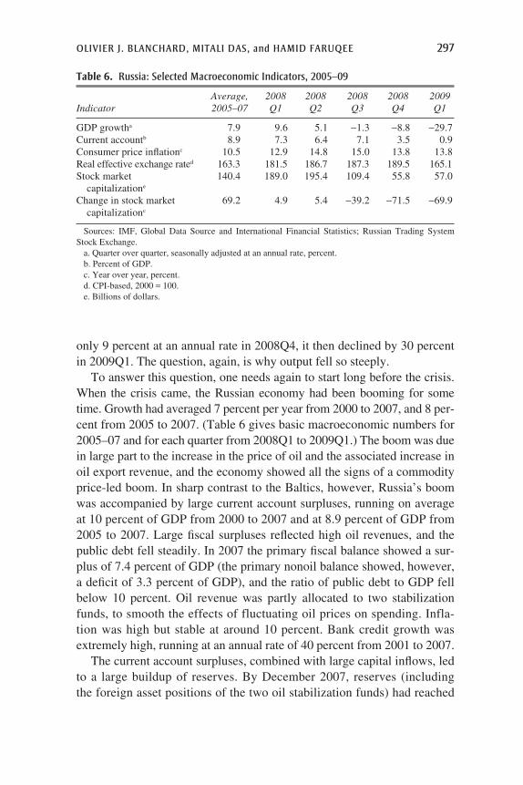
only 9 percent at an annual rate in 2008Q4, it then declined by 30 percentin 2009Q1. The question, again, is why output fell so steeply.

To answer this question, one needs again to start long before the crisis.When the crisis came, the Russian economy had been booming for sometime. Growth had averaged 7 percent per year from 2000 to 2007, and 8 per-cent from 2005 to 2007. (Table 6 gives basic macroeconomic numbers for2005–07 and for each quarter from 2008Q1 to 2009Q1.) The boom was duein large part to the increase in the price of oil and the associated increase inoil export revenue, and the economy showed all the signs of a commodityprice-led boom. In sharp contrast to the Baltics, however, Russia’s boomwas accompanied by large current account surpluses, running on averageat 10 percent of GDP from 2000 to 2007 and at 8.9 percent of GDP from2005 to 2007. Large fiscal surpluses reflected high oil revenues, and thepublic debt fell steadily. In 2007 the primary fiscal balance showed a sur-plus of 7.4 percent of GDP (the primary nonoil balance showed, however,a deficit of 3.3 percent of GDP), and the ratio of public debt to GDP fellbelow 10 percent. Oil revenue was partly allocated to two stabilizationfunds, to smooth the effects of fluctuating oil prices on spending. Infla-tion was high but stable at around 10 percent. Bank credit growth wasextremely high, running at an annual rate of 40 percent from 2001 to 2007.

The current account surpluses, combined with large capital inflows, ledto a large buildup of reserves. By December 2007, reserves (includingthe foreign asset positions of the two oil stabilization funds) had reached


Table 6. Russia: Selected Macroeconomic Indicators, 2005–09


GDP growtha 7.9 9.6 5.1 −1.3 −8.8 −29.7Current accountb 8.9 7.3 6.4 7.1 3.5 0.9Consumer price inflationc 10.5 12.9 14.8 15.0 13.8 13.8Real effective exchange rated 163.3 181.5 186.7 187.3 189.5 165.1Stock market 140.4 189.0 195.4 109.4 55.8 57.0

capitalizatione

Change in stock market 69.2 4.9 5.4 −39.2 −71.5 −69.9capitalizationc

Sources: IMF, Global Data Source and International Financial Statistics; Russian Trading SystemStock Exchange.

a. Quarter over quarter, seasonally adjusted at an annual rate, percent.b. Percent of GDP.c. Year over year, percent.d. CPI-based, 2000 = 100.e. Billions of dollars.


$480 billion, equivalent to 36 percent of GDP. Total foreign debt was$464 billion, of which $114 billion reflected loans to banks, $42.6 billionforeign deposits in banks, and $210 billion loans to households and firms.Of this debt, $361 billion was denominated in foreign currency, and$100 billion was short-term debt.

With a large current account surplus, a large fiscal surplus, a smoothingmechanism against oil price fluctuations, nearly no public debt, and a ratioof reserves to short-term debt equal to over 480 percent, one would haveexpected Russia to manage the crisis well. This was not the case.

The trade shock was severe. The dominant channel was not so much thedecrease in export volumes as the decrease in oil prices, which fell from$138 per barrel in July 2008 to $44 per barrel in early 2009. The terms oftrade for Russia’s overall commodity exports, which accounted for a verylarge 22 percent of GDP, fell 36 percent during the crisis semester relativeto the previous semester. The decline in our terms of trade variable was thethird largest in our sample, exceeded by only Venezuela and Chile. Theinteresting question is whether, given the presence of stabilization funds,the terms of trade decrease had a large adverse effect on demand. Putanother way, given that most of Russia’s oil revenue goes to the state, wasthe decline in revenue reflected in fiscal tightening? The answer is not obvi-ous. The increase in the fiscal deficit in 2008Q4 far exceeded the decreasein oil revenue. But this increase was followed by a sharp decrease in thedeficit in 2009Q1, while oil revenue was decreasing further. This wouldsuggest a positive effect on demand in 2008Q4 but a strongly adverseeffect in 2009Q1, which could help explain the large decline in output inthat quarter. What complicates the matter is that Russia typically experi-ences large fiscal deficits in the fourth quarter for seasonal reasons. Thus,the relevant question is whether the deficit was larger than expected, andthis we cannot answer. A strong fiscal stimulus program was put in placein April 2009, too late to have an effect on the period under consideration.

The post-Lehman financial shock was not the first such shock experi-enced by Russia in 2008. The first, triggered by the war with Georgia,came in August: large portfolio withdrawals led to a 22 percent decline inthe stock market from the start of the war in early August to just beforethe collapse of Lehman and gross outflows of $20 billion. The same hap-pened after Lehman: the stock market declined by 17 percent in two days,after which the Russian authorities closed it for two days.

The initial reaction of the Russian central bank was twofold. First, itsought to use reserves to limit the size of the depreciation and avoid balancesheet effects. (Figure 12 shows the path of reserves and of the exchange



rate from December 2007 to June 2009.) The second was to provide rubleliquidity to banks, through a decrease in reserve requirements, the provi-sion of uncollateralized loans to a larger set of banks, and the provision of$50 billion to the large state bank, VEB, to help firms repay their externaldebt. More exotic measures were taken as well, such as the allocation ofroughly $5 billion from the National Reserve Fund to buy shares, in order toincrease the value of the collateral (often their own shares) posted by firms.

Despite these measures, outflows continued at a rapid pace, and theRussian central bank steadily lost reserves: $25 billion in September,$72 billion in October, $29 billion in November, and $29 billion inDecember. (Table 7 reports the current account, the financial account, andreserves as averages for 2005–07 and for each quarter from 2008Q1 to2009Q1.) Why were outflows so large? For the most part, because investorsperceived that the rate of loss in reserves was too high to be sustained, andthus anticipated a larger depreciation to come. Domestic firms repaid theirdollar loans. Domestic depositors shifted from ruble to dollar accounts;the share of foreign currency–denominated bank deposits increased from14 percent in September to 27 percent in December. Domestic banksshifted from making domestic loans to buying dollar assets, in amountsbeyond what was needed to hedge the change in the currency structure of


Figure 12. Russia: Reserves and the Exchange Rate

Sources: IMF, International Financial Statistics; Bloomberg L.P.a. Daily data, inverted scale.

Billions of dollars Rubles per dollar

100

200

300

400

500

600

700

MayJan MarNovSepMay2008

Oil price peak

Reserves (left scale)

Exchange ratea

(right scale)

2009JulMarJan

25

30

35

40

Lehmancollapse

“Controlled”devaluation


their liabilities. (In view of the expected depreciation, the demand for dol-lar loans was obviously low.) By mid-November the Russian central bankdecided to widen the exchange rate band and allow for a faster deprecia-tion. The ruble was devalued by about 20 percent in January 2009, largelyending the net outflows and reserve losses.

By then, however, it was too late to avoid an output decline. Despite theprovision of liquidity, doubts about solvency had increased the interbankrate from 4 percent in July 2008 to 16 percent in January 2009. Over thesame period, the shift by banks from domestic loans to dollar assets wasreflected in an increase in the average interest rate charged to firms from11 percent in July 2008 to 17 percent. Credit to households, which hadgrown by 3 percent monthly from January to September 2008, remainedflat for the rest of the year and then decreased by 1 percent monthly fromJanuary 2009 on. Credit to firms, which had grown by 2.6 percent monthlyfrom January to September 2008, actually increased further to 3.5 percentmonthly from October to January, in some measure because of govern-ment pressure on state banks to increase credit, as well as a strong desire offirms to replace dollar debt with ruble debt. It then remained flat from Jan-uary on, in part because firms began to repay debt they had assumed duringthe crisis, as the ruble began to appreciate.

In short, Russia was affected by two shocks, a terms of trade shock anda financial shock. One might have hoped that the existence of the stabiliza-tion funds for oil would limit the adverse effects on demand of the decrease


Table 7. Russia: Current Account, Capital Flows, and Reserves, 2005–09Billions of dollars


Exports of goods and servicesa 364.0 136.0 156.9 167.2 121.9 74.4Imports of goods and servicesa −276.5 −97.2 −130.6 −136.5 −112.2 −64.7Current account balanceb 85.4 38.0 26.2 29.7 8.5 9.3Net bank flows 20.5 −11.3 22.1 −13.2 −51.4 0.5Net nonbank financial flows 12.5 −14.2 12.8 3.5 −84.4 −32.7Financial account balancec 33.0 −25.6 34.9 −9.8 −135.9 −32.2Exceptional financing from −1.2

IMFChange in reservesd 71.4 6.4 64.2 15.0 −131.1 −30.5

Source: IMF, International Financial Statistics.a. Includes factor income flows.b. Includes transfers.c. Excludes changes in reserves and official (IMF) financing.d. Differs from the sum of the current account balance, the financial account balance, and official

financing due to errors and omissions (not shown).


in oil prices. One might also have hoped that the initial high reserves andlow debt positions would limit the effects of the financial shocks. This wasnot the case, and the story has an interesting twist: the problems did notcome so much from capital outflows by foreign investors as from a shiftby domestic residents—households, firms, and banks—out of ruble andinto dollar assets. In this sense Russia may be the country that most corre-sponds to the case considered by Maurice Obstfeld, Alan Taylor, and JayShambaugh (2010), who argue that the variable to which reserves shouldbe compared is not short-term debt, but rather total liquid assets held bydomestic residents. At the start of the crisis, short-term debt in Russia wasabout $100 billion, but M2 was about $430 billion, much closer to thenumber for reserves. Given the ease with which domestic residents couldshift into dollar assets, this may be why it was rational to expect a depreci-ation, and the equilibrium was self-fulfilling.

Russia’s experience also exemplifies the dangers of pegging (or, moreaccurately, of sharply limiting the decline in the currency) when otheractors expect the policy to come to an end and the currency to depreciate.One can question whether, ex ante, Russia’s policy was mistaken. Ex ante,it was plausible that the crisis would come to an end sooner, that oil priceswould recover, and that reserves would prove more than sufficient. Also(and this is the other side of the same coin), the controlled depreciationallowed firms to decrease their foreign currency exposure and thus suffersmaller balance sheet effects when the depreciation actually came. Onecan also ask whether a Federal Reserve swap line like those extended toMexico, Korea, and Brazil would have allowed Russia to credibly main-tain its exchange rate and reduce its capital outflows.

III.C. Chile and the Role of Institutions

Like Russia, Chile depends very much on commodity exports—inChile’s case, copper—and is financially open. Yet it suffered a relativelysmall decline in output: −10 percent in 2008Q4 and −4 percent in 2009Q1(again at annual rates). The question this time is why the decline was somodest.

Chile entered the crisis in strong macroeconomic shape. From 2005 to2007 growth was steady, averaging 4.5 percent per year. This performancereflected in part Chile’s strong dependence on copper—copper exportswere 23 percent of GDP in 2007—and the doubling of the price of copperbetween 2005 and 2007. Strong copper exports led to large trade and cur-rent account surpluses. Inflation was stable, at least until 2008 when itstarted to increase, leading to a steady increase in the policy interest rate



from 5 percent in January to 8.15 percent in September. (Table 8 givessome basic macroeconomic numbers for Chile.)

The country’s balance sheets, both public and private, were strong. Theeffects of copper prices on the fiscal balance, and thus on aggregatedemand, were smoothed by a fiscal rule setting annual spending in line withmedium-term revenue, including copper revenue, under a conservative cop-per price assumption. The surplus was accumulated in a stabilization fund,which by 2007 had accumulated $15 billion. (GDP that year was $164 bil-lion.) Public debt, including debt of public enterprises, was a low 24 per-cent of GDP. For 2007 the primary balance showed a surplus of 8.8 percentof GDP, 0.2 percent excluding mining. Private foreign debt, owed mostlyby individuals and firms rather than banks, was $56 billion. The bankingsector was heavily regulated and strong, reflecting lessons learned in ear-lier banking crises. Subsidiaries of foreign banks accounted for roughlyhalf of total bank assets. Central bank reserves were $24 billion, roughly75 percent of the country’s short-term debt. (Beginning in April 2008, inthe face of higher global risk, the central bank had started a reserve accu-mulation program. By the time the program ended in September, it hadaccumulated $5.75 billion.)

The main effect of the crisis was through the trade channel. The crisiswas associated with a decrease in exports but also, and more important,with a sharp decline in the price of copper. The decline in our terms oftrade measure for Chile was the second largest of the countries in our sam-ple (after Venezuela), and only marginally larger than Russia’s. Given thecountry’s fiscal rule, the effect on disposable income and demand was lim-


Table 8. Chile: Selected Macroeconomic Indicators, 2005–09


GDP growtha 4.5 6.7 6.5 −1.4 −9.8 −4.3Current accountb 3.5 0.5 0.4 −4.5 −5.7 0.0Consumer price inflationc 3.6 8.0 9.0 9.3 8.5 5.9Real effective exchange rated 93.8 102.9 100.3 94.0 85.2 91.4Stock market capitalizatione 178.0 241.4 200.8 177.7 132.7 149.7Change in stock market 21.1 15.1 −15.7 −22.8 −41.3 −38.0

capitalizationc

Sources: IMF, Global Data Source and International Financial Statistics; Santiago Stock Exchange.a. Quarter over quarter, seasonally adjusted at an annual rate, percent.b. Percent of GDP.c. Year over year, percent.d. CPI-based, 2000 = 100.e. Billions of dollars.


ited, however; instead the decrease showed up in a sharp decline in accu-mulations of the stabilization fund, from $3 billion in 2008Q1 to $1 billionin 2008Q4. In 2009Q1 the government put in place an additional fiscalstimulus program of $4 billion; financing needs increased further later inthe year by another $4 billion.

On the financial side, what is most striking is that net capital flowsactually remained positive in both 2008Q4 and 2009Q1. (Table 9 reportsthe current account, the financial account, and reserves as averages for2005–07 and for each quarter from 2008Q1 to 2009Q1.) Thus, despite asharp decrease in the current account balance, the decrease in reserves wassmall—$1 billion in 2008Q4, followed by an increase of $0.5 billion in2009Q1—and associated with a moderate depreciation: the real exchangerate index fell from 100 in 2008Q2 to 85 in 2008Q4 and then recovered to91 in 2009Q1.

This behavior of reserves and the exchange rate was probably due totwo main factors. The first was the central bank’s decision to allow theexchange rate to adjust rather than to use the policy interest rate or to relyon reserve decumulation. Only in January 2009, after inflation had sub-stantially declined, was the policy rate lowered, by almost 500 basis pointsbetween January and March 2009. Starting at the end of September, thecentral bank made some dollar liquidity available to banks, but at a fairlylarge spread (300 basis points initially) over LIBOR.

The second factor was the behavior of gross capital flows. Gross out-flows were only marginally higher during the two quarters of the crisis


Table 9. Chile: Current Account, Capital Flows, and Reserves, 2005–09Billions of dollars


Exports of goods and servicesa 67.9 23.5 22.7 20.7 16.4 15.1Imports of goods and servicesa −65.4 −22.6 −23.9 −24.3 −19.0 −14.5Current account balanceb 5.3 1.5 0.1 −2.9 −2.1 0.9Net bank flows 0.2 1.6 1.2 0.1 −1.1 −2.1Net nonbank financial flows −4.1 −1.1 1.0 7.5 2.8 2.9Financial account balancec −3.9 0.5 2.2 7.6 1.7 0.8Change in reservesd 1.2 0.4 2.4 4.6 −0.9 0.5

Sources: IMF, International Financial Statistics.a. Includes factor income flows.b. Includes transfers.c. Excludes changes in reserves and official (IMF) financing.d. Differs from the sum of the current account balance, the financial account balance, and official financ-

ing due to errors and omissions (not shown).


than before. Interestingly, gross inflows increased even more. These inflowscame not only from the repatriation of funds by pension funds but also,indeed to a larger extent, from domestic firms and households. This is insharp contrast to what happened, for example, in Russia, where capital out-flows by foreign investors led to capital outflows by domestic residents.How much was due to the decision to let the peso depreciate (in contrastwith Russia, which tried to maintain a peg despite the anticipation byinvestors of a future devaluation) and how much was due to the perceptionof Chile as a relatively safe financial haven is difficult to assess. The result,in any case, was only a small loss in reserves and a moderate depreciation.

Nevertheless, the trade shocks and the financial crisis had some effecton the real economy. The stock market fell by almost 15 percent from Sep-tember to December, a small decrease relative to other emerging marketcountries. And although the interbank rate rose little relative to the policyrate, there was an increase in lending rates of roughly 4 percentage pointsfrom September to December, at a time when, in addition, inflation wasfalling, implying a larger increase in real interest rates.

The overall result was a decrease in demand and in output, but on a morelimited scale than in many other countries. The fiscal rule, the frameworkfor smoothing the effect of copper revenue, a strong financial sector, lim-ited foreign currency exposure, and the decision early on to let the pesodepreciate probably all played a role in the outcome.

IV. Conclusions

One can read the three preceding sections as first building the bone structureand progressively adding the flesh. The model presented in section I hasallowed us to identify and analyze the effects of the main two shocks thataffected emerging market countries during the crisis: a sharp decrease inexports (together with a sharp decrease in the terms of trade for commod-ity producers), and a sharp increase in capital outflows. It showed thedependence of the unexpected output losses on initial conditions, in partic-ular on foreign debt. It showed the complexity of the decisions policymak-ers faced in this environment, and the effects of using the policy interestrate, the exchange rate, reserve decumulation, and fiscal policy.

The econometrics in section II provided a first pass at the data. Despitethe limitations inherent in using a cross-sectional dataset with only 29observations, our empirical analysis yielded strong evidence that both thetrade and the financial channel played important roles. The differing effectsof the shocks across countries, coming from different trade and financial



exposures and the differing growth performances of countries’ tradingpartners, explain much of the heterogeneity of growth performances dur-ing the crisis. When it comes to policy, our most interesting findings aretwo “nonresults.” Countries with fixed exchange rate regimes fared, onaverage, much worse. However, when we control for other factors, in par-ticular short-term debt, the direct effect of fixed exchange rates largely dis-appears. This finding is consistent with the ambiguous effect of exchangerates in our model: the outcome depends on the strength of expenditureswitching and balance sheet effects. We did not find compelling economet-ric evidence that international reserves were important buffers in the crisis.

The case studies give a better sense of the many factors that shaped theeffects of the crisis in each country, which cannot be captured by econo-metrics alone. The comparison between Russia and Chile is perhaps themost interesting. Both countries are large commodity producers, and bothwere hit by a large adverse trade shock. Both were financially open. Russiahad larger reserves relative to its short-term debt than Chile. Yet Chile wasmuch less affected by the crisis than Russia. The proximate reasons forChile’s relative success are probably twofold. First, Chile used its fiscal sta-bilization mechanisms more effectively than Russia did. Second, whereasChile experienced small capital outflows by foreigners and more than off-setting capital inflows by domestic residents, Russia suffered large capitaloutflows by both foreigners and domestic residents. The deeper reasons forthese differences in capital flows are probably the greater confidence in themacrofinancial structure in Chile than in Russia, and Chile’s decision earlyon to let its currency depreciate, which compares favorably with Russia’sinitial decision, eventually abandoned, to maintain the parity, giving rise tospeculative outflows.

ACKNOWLEDGMENTS We are indebted to Nese Erbil and DavidReichsfeld for superb research assistance. We thank Brian Pinto, Irineu deCarvalho, Jorg Decressin, Kristin Forbes, Ayhan Kose, Hélène Rey, MatthewShapiro, Linda Tesar, and the editors for comments, and Chris Rosenberg,Pablo García, Julie Kozack, and Bas Bakker for very useful information anddiscussions. The views expressed in this paper are those of the authors and donot necessarily represent those of the International Monetary Fund.



References

Aizenman, Joshua. 2009. “Reserves and the Crisis: A Reassessment.” CentralBanking 19, no. 3: 21–26.

Aizenman, Joshua, and Yi Sun. 2009. “The Financial Crisis and Sizable Interna-tional Reserves Depletion: From ‘Fear of Floating’ to the ‘Fear of Losing Inter-national Reserves’?” Working Paper no. 15308. Cambridge, Mass.: NationalBureau of Economic Research (October).

Alessandria, George, Joseph P. Kaboski, and Virgiliu Midrigan. 2009. “The GreatTrade Collapse of 2008–09: An Inventory Adjustment?” Working Paperno. 10-18. Federal Reserve Bank of Philadelphia.

Anderton, Robert, and Tadios Tewolde. 2010. “Financial Turmoil, the GlobalTrade Downturn, and Global Production Chains.” Frankfurt: European CentralBank.

Auboin, Marc. 2009. “Restoring Trade Finance during a Period of Financial Cri-sis: Stock-Taking of Recent Initiatives.” Staff Working Paper ERSD-2009-16.Geneva: World Trade Organization (December).

Bakker, Bas, and Anne Marie Gulde. 2009. “The Credit Boom in EU New Mem-ber States: Bad Luck or Bad Policies?” IMF Working Paper 130. Washington:International Monetary Fund.

Berglof, Erik, Yevgeniya Korniyenko, and Jeromin Zettlemeyer. 2009. “Under-standing the Crisis in Emerging Europe.” EBRD Working Paper no. 109. Lon-don: European Bank for Reconstruction and Development (November).

Berkmen, Pelin, Gaston Gelos, Robert Rennhack, and James P. Walsh. 2009. “TheGlobal Financial Crisis: Explaining Cross-Country Differences in the OutputImpact.” IMF Working Paper 280. Washington: International Monetary Fund(December).

Céspedes, Luis Felipe, Roberto Chang, and Andrés Velasco. 2004. “Balance Sheetsand Exchange Rate Policy.” American Economic Review 94, no. 4: 1183–93.

Freund, Caroline. 2009. “The Trade Response to Global Downturns: HistoricalEvidence.” World Bank Policy Research Working Paper no. 5015. Washing-ton: World Bank.

Ghosh, Atish R., Jonathan David Ostry, and Chanalambos G. Tsangarides. 2010.“Exchange Rate Regimes and the Stability of the International Monetary Sys-tem.” IMF Occasional Paper 270. Washington: International Monetary Fund.

Giannone, Domenico, Michele Lenza, and Lucrezia Reichlin. 2009. “Market Free-dom and the Global Recession.” Paper presented at a conference on EconomicLinkages, Spillovers and the Financial Crisis, organized by the InternationalMonetary Fund and the Banque de France chair of the Paris School of Econom-ics, Paris, January 29. www.imf.org/external/np/res/seminars/2010/paris/.

IMF. 2010. “How Have Emerging Markets Coped with the Crisis?” Strategy,Policy, and Review Department (forthcoming).

Kannan, Prakash, and Fritzi Köhler-Geib. 2009. “The Uncertainty Channel ofContagion.” IMF Working Paper 219. Washington: International MonetaryFund.



Lane, Philip R., and Gian Maria Milesi-Ferretti. 2010. “The Cross-CountryIncidence of the Global Crisis.” Washington: International Monetary Fund(January).

Levchenko, Andrei A., Logan T. Lewis, and Linda L. Tesar. 2009. “The Collapseof International Trade during the 2008–2009 Crisis: In Search of the SmokingGun.” Working Paper no. 16006. Cambridge, Mass.: National Bureau of Eco-nomic Research.

Obstfeld, Maurice, Alan M. Taylor, and Jay C. Shambaugh. 2010. “Financial Sta-bility, the Trilemma, and International Reserves.” AEJ Macro 2, no.2: 57–94.

Patillo, Catherine, Hélène Poirson, and Luca Ricci. 2002. “External Debt andGrowth.” IMF Working Paper 69. Washington: International Monetary Fund.

Rose, Andrew, and Mark Spiegel. 2009a. “Cross-Country Causes and Conse-quences of the 2008 Crisis: Early Warning,” NBER Working Paper no. 15357.Cambridge, Mass.: National Bureau of Economic Research.

———. 2009b. “Cross-Country Causes and Consequences of the 2008 Crisis:International Linkages and American Exposure.” Working Paper no. 2009-18.Federal Reserve Bank of San Francisco.

Sommer, Martin. 2009. “Why Has Japan Been Hit So Hard by the Global Reces-sion?” IMF Staff Position Note SPN/09/05. Washington: International MonetaryFund.

Trivedi, Kamakshya, and Swarnali Ahmed. 2010. “Reserves and the EM CrisisExperiences—A Mixed Blessing.” Global Economics Weekly (March 10).

Von Furstenberg, George M. 2003. “Price Insurance Aspects of Monetary Union.”Journal of Common Market Studies 41, no. 3: 519–39.

Yi, Kei-Mu, Rudolfs Bems, and Robert C. Johnson. 2009. “The Role of VerticalLinkages in the Propagation of the Global Downturn of 2008.” Paper presentedat a conference on Economic Linkages, Spillovers and the Financial Crisis,organized by the International Monetary Fund and the Banque de France chairof the Paris School of Economics, Paris, January 29. www.imf.org/external/np/res/seminars/2010/paris/.



308

Comments and Discussion

COMMENT BYKRISTIN J. FORBES This paper by Olivier Blanchard, Mitali Das, andHamid Faruqee asks a well-defined and extremely important question: howdid the recent crisis affect emerging markets in late 2008 and early 2009?The answer has critical policy implications both for emerging marketsand for the international financial institutions. To answer this question, thepaper begins with an intuitive model that clearly lays out the main chan-nels by which the crisis could affect emerging markets, and the effects ofdifferent policy responses. Then it reports a series of regressions to testthe role of various channels in explaining the spread of the crisis, focusingon the role of trade versus that of finance and the impact of macroeconomicpolicies. The paper closes with several case studies, which provide impor-tant detail on the cross-country regression results—and show the challengesin generalizing about emerging market experiences during the crisis.

This paper should be required reading for anyone attempting to under-stand how emerging markets were affected during the peak of the crisis. Itis straightforward to read and understand and does an excellent job ofarticulating a model to frame the issues and then evaluating the predictionsof the model through cross-country analysis and more in-depth countrystudies. Both approaches clearly benefit from the authors’ mix of academicknowledge and real-world experience. The regression analysis carefullytests a variety of alternative hypotheses and measures, and the resultsare surprisingly strong given the limited degrees of freedom available. Themost robust findings are that the crisis spread to emerging markets throughboth the trade and the financial channels, but with a more important rolefor finance, as measured by countries’ exposure to short-term external debt.This result is logical and supports anecdotal evidence gathered during thecrisis as well as the more detailed analysis in the case studies. The results

12178-05b_Blanchard comments_rev1.qxd 8/11/10 12:17 PM Page 308

also suggest that neither exchange rates nor reserve accumulation had muchof a direct effect in determining how the crisis affected emerging markets.These results have important policy implications.

The authors have also done an impressive job in addressing many ofthe concerns that were raised when they presented a draft of this paper at the Brookings Papers conference. My comments will therefore focuson only four issues: the dependent variable, the sample size, omitted vari-ables, and the assumptions about capital flows. These issues are not newto the authors—indeed, they are very candid about the limitations of theirdata and analysis.

Let me begin by highlighting one important innovation that was alreadypresent in the conference version and has been further improved in thisversion. The earlier version did not focus on explaining growth in emerg-ing markets during the whole of 2008 or 2009, although this is the standardmeasure used in other, related papers and would have been straightforwardto measure. Instead it attempted to explain the difference between growthduring the peak semester of the crisis (2008Q4 and 2009Q1) and trendgrowth (average growth from 1995 through 2007).

This measure of the dependent variable was better than that used inother work, not only because it focused on the change in growth versus thetrend, but also because it focused on growth during the peak of the crisisrather than over an entire year. Growth in many countries was strong bothat the start of 2008 and at the end of 2009, so that focusing on annualgrowth could have missed the full impact of the crisis. This measure, how-ever, still had the shortcoming of overstating the impact of the crisis oncountries that were already expected to have slower growth in 2008Q4 or2009Q1 for reasons unrelated to the crisis. (For example, annual growth inLatvia was already expected to slow from a trend rate of 8.8 percent from2000 to 2007 to 3.6 percent in 2008, before any effect of the crisis, accord-ing to IMF data.) The published version of the paper adjusts for this byfocusing on “unexpected growth”—the forecast error for output growthduring the 2008Q4–2009Q1 semester—instead of growth versus trend.This choice of measure should more accurately capture how the crisischanged growth in these countries, which is the key variable of interest.

One challenge resulting from this choice of measure of the growthshock, however, is that the available data are limited. Quarterly growthdata are not available for many emerging markets and other developingcountries, and several of the remaining countries lack the necessary fore-cast data, so the main regressions have a maximum of 29 observations.Many emerging markets are omitted from the sample, such as Bahrain,

COMMENTS and DISCUSSION 309


Bangladesh, Bolivia, Botswana, the Dominican Republic, Ecuador, Egypt,El Salvador, Jamaica, Jordan, Kazakhstan, Kuwait, Morocco, Pakistan,Romania, Singapore, Uruguay, and Vietnam. Moreover, the sample isdominated by countries in Eastern Europe—just over one-third of the sam-ple is from this region. In comparison, more traditional emerging marketsamples that do not rely on quarterly data generally have less than 20 per-cent of the sample from Eastern Europe. Moreover, this unbalanced sampleis not random, because the overrepresentation of Eastern Europe resultsfrom requirements on EU members to report quarterly data.

The authors are candid about this shortcoming with the sample size andcareful not to ask too much of the data, given the limited degrees of free-dom. Nonetheless, the small sample raises questions about whether theresults are driven by outliers or by patterns in Eastern Europe or othersmall groups of countries that may not apply to the full set of countries.My table 1 reports several tests to see whether this is important. I focus onthe main regression results in column 1-2 of the authors’ table 1, in whichthe trade channel is measured by unexpected growth in trading partnersand the financial channel by short-term external debt. The first columnin my table replicates the results in the paper. The second column clusterserrors by region—which, one could argue, is the preferred method of esti-mation. This increases the significance of the trade variable, and the finan-cial variable remains significant. The next column then drops Eastern


Table 1. Regressions Explaining GDP Growth in Emerging Market Countriesa

Full sampleSample Sample

Errors Errors omits omits Estonia,not clustered by Eastern Latvia, and

Independent variable clustered regionb Europec Lithuania

Unexpected growth in 0.732* 0.732** 0.783 0.659*partner countries (0.374) (0.184) (0.454) (0.371)

Short-term external debt −0.279** −0.279** −0.463 −0.265* (0.044) (0.041) (0.322) (0.135)

No. of observations 29 29 19 26Adjusted R2 0.46 0.46 0.24 0.21

Source: Author’s regressions.a. The dependent variable is unexpected GDP growth in 2008Q4 and 2009Q1, defined as the difference

between actual growth and the International Monetary Fund’s April 2008 forecast; all growth rates areannualized. Except where stated otherwise, the sample consists of the 29 countries included in the mainregressions in Blanchard, Das, and Faruqee (this volume). Numbers in parentheses are standard errors.Asterisks indicate statistical significance at the *10 percent and the **5 percent level.

b. Regions are Eastern Europe, Asia, Latin America, and other.c. The omitted countries are Croatia, Czech Republic, Estonia, Hungary, Latvia, Lithuania, Poland,

Serbia, Slovak Republic, and Slovenia.


Europe from the sample. The coefficients on both the trade and the finan-cial variables are now insignificant. This suggests that patterns in EasternEurope may be driving the results, but because the sample size is now sosmall, it may be too much to expect statistically significant results. Tomaintain a larger sample and some representation of Eastern Europe, thelast column drops just three countries—Estonia, Latvia, and Lithuania—that appear to be outliers when residuals are plotted. Now the coefficientson partner growth and short-term debt are both borderline significant (at the10 percent level), suggesting that these three countries in Eastern Europemay be important in driving the results.

This series of results suggests that it may be worth expanding the sam-ple size to ensure that the results are not driven by a small subset of coun-tries or by the specific characteristics of Eastern Europe. Of course, thisis much easier said than done. One solution would be to continue usingquarterly growth data, but to add countries that are traditionally classi-fied as developed even though they share some characteristics withcountries in the emerging market sample. For example, why not includeGreece, Iceland, Italy, Portugal, and Spain? Income per capita in each ofthese countries is about the same as in Israel, Slovenia, or Taiwan—all ofwhich are in the sample and are generally classified as emerging mar-kets. The challenge in including these Western European countries maybe political, in the sense that they might not appreciate being classifiedas “emerging markets”—especially by a group of authors from the Inter-national Monetary Fund.

A related issue to consider when interpreting the results is the possibil-ity of omitted variables. The literature on contagion suggests a number ofother mechanisms by which the crisis could have affected emerging mar-kets (see Claessens, Dornbusch, and Park 2001). For example, the paperinterprets the significant negative coefficient on short-term debt as show-ing the importance of the financial channel in spreading the crisis. But isthere an omitted variable, correlated with short-term debt, that actually drives this relationship? For example, are countries that are riskier andmore vulnerable more likely to have higher short-term debt ratios? Proba-bly. And wouldn’t these more risky and vulnerable countries be morelikely to experience a large growth slowdown during the crisis as risk aver-sion increases—independent of their share of short-term debt? Similarly,other work on contagion has discussed how trade can spread crises throughdifferent effects, for example by affecting import demand and competitive-ness (see Forbes 2004). The paper tests its measures of the trade channelindividually, but it should test them simultaneously along with the various



financial measures. Of course, the challenge in controlling for many ofthese factors simultaneously is again the small sample size, which againunderscores the importance of extending the sample to more countries.

My final comment relates to the authors’ model and its relationship tothe empirical results. In the model, net capital inflows depend on the EMBIspread adjusted for a risk premium and home bias. A key assumption isthat an increase in perceived risk or an increase in home bias causesinvestors and financial institutions in developed countries to reduce theirforeign lending and thereby reduce net capital flows to emerging markets.This assumption is critical for the analysis. The reduction in net capitalflows that results from an increase in home bias (assuming a given policyrate and unchanged reserves) reduces the trade balance, causes the homecurrency to depreciate, and lowers output. The model yields similar resultsif there is an increase in risk aversion: net capital flows and output againdecline, although the effect on the exchange rate is ambiguous.

But how valid is the assumption that when the crisis hits, the result is necessarily to reduce net capital flows? This has been the standardassumption in a large literature on “sudden stops,” which argues that dur-ing crises, capital flows to emerging markets suddenly cease (see Calvo1998). But there has been little formal testing of this hypothesis. Theauthors deserve credit for at least mentioning that this assumption maynot hold in all cases, although they leave exploring the ramifications forthe model and the empirical analysis for future work. Moreover, the casestudy on Chile provides a clear example of an emerging market wherethis assumption does not hold—a great example of the benefits of doingdetailed case studies.

But is this pattern of increasing rather than decreasing net capitalinflows unique to the Chilean experience, or is it a broader phenomenon?My figure 1 shows gross capital inflows and outflows and the resulting netcapital flows for the United States during the crisis. (I focus on the UnitedStates because data distinguishing gross flows by domestic from those byforeign investors are readily available.) The figure shows that gross capitalinflows from foreigners fell in late 2008. At the same time, however, grosscapital outflows by domestic investors were negative, suggesting that theybrought home large amounts of capital previously invested abroad. As aresult, net capital flows into the United States actually increased duringthis period. Granted, the United States is not an ideal comparator, as it is adeveloped country with large and liquid capital markets, which may havebecome relatively more attractive to investors during the crisis. The exam-ple does show, however, that changes in investment by domestic residents



can easily overwhelm changes by foreigners and lead to a net increaseinstead of a net decrease in capital flows during a crisis.

Do any countries other than the United States and Chile exhibit this pat-tern? As a rough test, I examine a group of 101 countries to see whether netcapital flows in 2008Q4 were larger or smaller than in 2007Q4.1 Table 2shows that in the full sample, net capital flows increased in 45 countries butdecreased in 56. Many of the countries in which capital inflows increased,however, are developed countries. The last row of the table therefore looksat the patterns for emerging markets only; it shows that emerging marketswere more likely to see a decrease in net capital flows than an increase dur-ing the crisis. This “sudden stop” is apparent in many of the major emergingmarkets, including Argentina, Brazil, Peru, Poland, Russia, South Africa,and Turkey. But the table also shows that the pattern of increasing insteadof decreasing net capital inflows is not unique to Chile among developingcountries. In fact, even many countries in the authors’ sample—includingColombia, the Czech Republic, Israel, Mexico, and Thailand—experienceda net increase in net capital flows in 2008Q4 over 2007Q4, contradictingtheir model’s key assumption.


1. The sample includes all countries for which data were available. I focus only on thefourth quarter because, as of this writing, data for 2009Q1 are not as widely available, andonly by comparing similar quarters can one control for seasonal effects that can significantlyaffect capital flows.

Figure 1. United States: Capital Inflows and Outflows, 1970–2008

Trillions of dollars

Source: Bureau of Economic Analysis.

–1.5

–1.0

–0.5

0

0.5

1.0

1.5

2.0

20052000199519901985198019751970

U.S. purchases of foreign assets

Net capital flows

Foreign purchases of U.S. assets


Given that this key assumption of the model does not appear to holdfor a number of countries, many of its key predictions might not applyto this subset of countries. For example, for countries with net capitalinflows during the peak of the crisis, the financial channel would not beexpected to have as large an effect. To test this, it would be straightfor-ward to repeat the main regression analysis but split the sample into twogroups: those with net capital inflows (or at least not large outflows),and those with large net capital outflows. Given the small sample size,this would certainly be pushing the degrees of freedom, but it couldshow very different effects of the crisis for these two subsamples ofemerging markets.

To conclude, this paper addresses a very important question: how didthe crisis spread to emerging markets? It does an excellent job of layingout the key issues and testing several different hypotheses. It takes painsto evaluate several different theories but is challenged by the very starklimitations of the data—especially the small sample size, which makes itdifficult to control for various effects and relationships simultaneously.Nonetheless, the empirical results seem fairly robust, especially giventhe limitations of the exercise, suggesting that financial mechanismswere likely the most important factor in transmitting the crisis to emerg-ing markets during late 2008 and early 2009. Although this paper maynot be the last word on the issue, it presents convincing evidence onhow the crisis spread and should provide an excellent resource for any-one seeking to understand why a crisis that started in the U.S. subprimehousing market had such virulent effects in emerging markets aroundthe world.

REFERENCES FOR THE FORBES COMMENT

Calvo, Guillermo A. 1998. “Capital Flows and Capital-Market Crises: The Sim-ple Economics of Sudden Stops.” Journal of Applied Economics 1, no. 1(November): 35–54.


Table 2. Countries in Which Net Capital Flows Increased or Decreased from 2007Q4to 2008Q4

No. of countries

Sample Increase Decrease

Full sample 45 56Developed countries 14 7Emerging markets 31 49

Source: International Monetary Fund, International Financial Statistics.


Claessens, Stijn, Rudiger Dornbusch, and Yung Chul Park. 2001. “Contagion:Why Crises Spread and How This Can Be Stopped.” In International Finan-cial Contagion, edited by Stijn Claessens and Kristin J. Forbes. Norwell,Mass.: Kluwer Academic Publishers.

Forbes, Kristin J. 2004. “The Asian Flu and Russian Virus: The InternationalTransmission of Crises in Firm-Level Data.” Journal of International Econom-ics 63, no. 1: 59–92.

COMMENT BYLINDA L. TESAR1 The U.S. recession that began in late 2007 hadsignificant spillover effects on the rest of the globe. This paper by OlivierBlanchard, Mitali Das, and Hamid Faruqee studies the impact of the U.S.financial crisis and the accompanying economic contraction on 29 emerg-ing market countries in South America, the Middle East, Eastern Europe,and Asia. As figure 2 of the paper shows, the contraction experienced byemerging markets over the interval 2008Q4–2009Q1 was far from uniform.Lithuania, Latvia, Estonia, and Russia experienced “unexpected” economicgrowth rates (the difference between actual growth and the April 2008 IMFforecast) on the order of negative 25 percent, while Poland, Venezuela,and China experienced only mild declines. The objective of this paper is toexplain the heterogeneity in these negative growth rates. In particular, thepaper seeks to isolate which of two channels of transmission—openness totrade and openness to capital flows—is the more significant in accountingfor cross-country differences in growth rates during the crisis.

This is a thought-provoking paper on an important and timely issue. Itis well written and clear in its objective and in presenting its findings.The paper begins with a simple model of a small, open economy thattrades with the rest of the world and has access to international creditmarkets. The model is a highly stylized IS-LM framework—one thatabstracts from dynamics, expectations, and uncertainty—that the authorsuse to perform simple comparative static exercises. In this framework, adecrease in demand for a country’s exports or a shift away from its assetswill contract the aggregate budget constraint and, conditional on endoge-nous shifts in the exchange rate or adjustments in fiscal policy, will leadto a contraction in output.

The model motivates the regressions that are the core of the paper. Inessence, the authors run a horserace between various measures of openness


1. I thank the authors for making the data used in their paper readily available, and mystudent Logan Lewis for his help in analyzing the data.


in the current and the capital accounts on the cross section of unexpectedGDP growth rates in emerging markets during the two quarters of interest.The overall conclusion is that both channels played a role in global trans-mission, although the financial channel dominates in terms of statisticalsignificance and magnitude. Using the authors’ data, I was able to verifythat the core results are robust to changes in the specification of right-hand-side variables, sample selection, and other factors. My comments thereforefocus largely on the interpretation of the results and whether the takeawayfrom this paper is really as straightforward as the authors suggest.

THE THOUGHT EXPERIMENT. The premise of the paper is that emergingmarkets were the victims of a collapse in global demand for their goods andfor their financial assets. The shock that hit emerging markets is assumed tobe both external to the countries in the sample and common to all of them.The baseline regression implied by this thought experiment is a simpleone: the dependent variable is unexpected growth in GDP in each country,and the independent variables include measures of each country’s “expo-sure” to the shock: for example, trade as a share of GDP as a measure ofthe trade channel, and exposure to short-term debt for the financial chan-nel. Other right-hand-side variables are tested, and in general, the financialvariables come in significant and dominate the trade variables.

Of course, to conclude that the financial channel beats the trade channel,or even that the financial channel results are economically meaningful, onehas to impose the all-else-equal assumption. As is clear even in this simpleopen economy model, the transformation of a fall in foreign demand for acountry’s exports or its assets into a contraction in output depends on anumber of auxiliary assumptions about the structure of the economy. Ifcountries differ in the strength of their financial institutions, in the degreeof adjustment in goods prices or the exchange rate, or in elasticities ofsubstitution between home and foreign goods and between home and for-eign assets, to list just a few possibilities, the coefficients on the “trade”and the “finance” effects will differ across countries. In addition, there maybe endogenous policy responses to the shock, which would mitigate itseffects. Indeed, the bigger the exposure to the shock, the more likely othervariables such as prices will adjust, and the more likely governments willreact. What is effectively being estimated is the net effect of the shock onoutput, which results from a complicated mix of structural differencesacross countries and heterogeneous policy responses to shocks.

One could, in principle, control for some of these differences in order toisolate the “pure” trade and finance channels. The authors are well awareof the nature of the problem, and in a sense the model itself exposes the



various pitfalls in the regression analysis. Some controls are added to theregressions to try to address the issue, but one can only do so much in aregression with 29 observations. Therefore, the results should be viewed asa set of correlations between changes in output and external balances andnot as a set of causal relationships.

AN ALTERNATIVE INTERPRETATION. An alternative to the emerging-markets-as-victims scenario is that emerging markets, to a greater or lesser degree,rode the same credit boom that fueled the U.S. crisis. Low global inter-est rates, innovations in the banking sector, and rising real estate pricesresulted in an easing of credit and a boom in both private and public expen-diture in many countries. In this scenario the contraction in the second halfof 2008 was triggered not so much by a collapse in global demand as bythe global realization that the party was coming to an end.

The paper’s description of the sequence of events in Latvia in 2007and 2008 casts doubt on the emerging-markets-as-victims hypothesis.The case study of the Latvian crisis notes that “the right starting point isnot the start of the crisis itself, but the boom that the economy experi-enced in the 2000s.” Stock prices and real estate prices in Latvia soared inthe mid-2000s, and despite rising domestic goods and services prices,the country maintained its peg to the euro. Access to credit, with realestate as collateral, resulted in high rates of consumption and invest-ment growth. By early 2007, the paper notes, “signs of overheating and ofan impending bust were starting to become apparent.” In early 2008 GDPgrowth turned negative and asset prices began to fall—all of this wellbefore the external shocks of mid-2008.

Perhaps not surprisingly, the Latvian financial sector increasingly had toshift to shorter lines of credit. Figure 10 of the paper shows that Latvia hadthe highest ratio of short-term external debt to GDP of any emerging marketin the sample in 2007. This raises an important issue for the regressionanalysis. It is well known that as credit conditions tighten and risk assess-ments deteriorate, countries may become unable to borrow at long maturi-ties. Short-term debt is then no longer an exogenous variable revealing acountry’s exposure to external credit market conditions, but an endogenousmeasure of its own creditworthiness. It is not clear then whether the correctspecification is a regression of output growth on short-term debt or the otherway around. Again, absent a more complete structural model and the impo-sition of plausible identifying assumptions, the best one can do is concludethat the two variables are correlated.

The Latvian case also suggests that in order to separate the “victim ofexternal shocks” scenario from the “we got into the same trouble ourselves”



scenario, one can either use more country-specific information about thedynamics leading up to the contraction, or look carefully at the timing of theoutput collapse, or both. The collection of more country-specific informa-tion is beyond the scope of this paper, and certainly beyond the scope of thisdiscussion. However, it is fairly easy to look at the patterns in output in theperiod preceding that studied in the paper.

I show in figure 1 GDP growth rates for 27 emerging market countriesover two intervals: 2007Q4–2008Q1 and 2008Q4–2009Q1, the formerbeing the semester one year before that on which the paper focuses,


Figure 1. GDP Growth in 27 Emerging Market Countries, 2007Q4–2008Q1 and2008Q4–2009Q1

Source: Author’s calculations using International Monetary Fund data.

–25 –20 –15 –10

Percent

–5 0 5

2008Q4–2009Q12007Q4–2008Q1

ChileColombiaThailandIsraelIndonesiaSouth AfricaPolandPeruIndiaTaiwanKorea, Rep. ofArgentinaBrazilCzech Rep.MalaysiaMexicoSloveniaCroatiaHungaryEstoniaSlovak Rep.BelarusRussiaTurkeyLithuaniaLatviaBulgaria


and the latter the crisis semester itself. The countries are ranked by theirgrowth in GDP in the latter period, calculated using GDP volume datafrom the IMF. This differs a little from the dependent variable in the paper,which is the estimated deviation from the April 2008 IMF forecast. How-ever, the variable used in the regressions and the GDP growth rates calcu-lated here have a correlation coefficient of 0.73, so the message hereshould not be affected by the use of slightly different data. (The results ofthe basic regressions in the paper can also be replicated quite closely usingGDP volume data rather than the deviations-from-forecast series.)

The figure suggests that the cross section of growth rates in the secondsemester of 2007 is highly correlated with the cross section of growth ratesin 2008. In fact, the two sets of growth rates have a correlation coefficientof 0.93. This means that the countries with weak economic performance inthe last half of 2008, after experiencing the “external shock,” were thesame set of countries with weak performance in the last half of 2007,before the shock. Growth rates across the board were certainly lower in thelatter half of 2008 than in the latter half of 2007. But what the paper seeksto explain is the cross-sectional distribution of GDP growth—why somecountries fared so much worse than others—not why some countries havepersistently low growth rates. If this distribution is the same before andafter the shock, then it appears that one should be looking for longer-runreasons for differences in growth rates across countries and not the dif-ferential impact of a shock specific to the end of 2008.

Indeed, when the baseline regression is run including the growth ratefor the second semester of 2007 as a control, both the trade and the finan-cial variables lose their significance. Depending on the specification, someappear with the opposite sign. I am not suggesting that this is the mostappropriate test—a test symmetric to those in the paper would use the devia-tion of growth in 2007 from the forecast, and there are serious problems ofendogeneity in my regression. However, the fact that the regression is notrobust to including growth in 2007, together with the very high persistenceof growth rates, casts doubt on the empirical evidence that either the tradeor the financial channel is the primary explanation for the cross-sectionaldistribution of growth in emerging markets in the latter half of 2008.

Now, setting the empirical evidence in this paper aside, do I believethat emerging markets were affected by their openness to global markets?Absolutely. But I also believe that those economies benefited from access tothose markets in the period leading up to the crisis. The challenge remainswhat it was in the aftermath of previous emerging market crises: to developmodels capable of explaining the dynamics before, during, and after the



crisis, and then, through the lens of those models, propose policy tools thatcan help countries manage their exposure, in good times and in bad.

GENERAL DISCUSSION George von Furstenberg raised three points.First, with respect to the specification of the risk premium, severe posi-tive shocks to that premium were experienced by essentially all countrieswhether or not they had a collapsing housing bubble. Second, he was sur-prised that the authors were agnostic about whether the Marshall-Lernercondition holds in the long term for developing countries that generallyare obliged to price their exports to market. Third, he thought the paperneeded a better proxy for indebtedness effects.

Richard Cooper was troubled that the authors’ sample was too smallto allow for some necessary distinctions. He suggested thinking moreaggressively about expanding the list of countries, to include, for exam-ple, smaller countries like Costa Rica. Given the constraint imposed bythe need for quarterly GDP figures, he wondered whether the list couldbe enlarged by looking at industrial production for those countries thattypically report monthly or quarterly industrial production data. Fromthe estimated relationship between GDP and industrial production forthe countries that have both sets of data, one could then simulate quarterlyGDP data for those that do not.

Cooper also would have liked to see the paper distinguish between theimpact of trade shocks that initially fall on the government—the case formost oil-exporting countries, as well as Russia and Chile, two of the threecountries examined in the case studies—and that of shocks that initiallyfall on the private sector. He agreed with the authors’ position on theMarshall-Lerner condition. Although von Furstenberg’s point was valid, ifa country has a large external debt denominated in foreign currency, then,starting from a current account deficit, it is very easy to imagine circum-stances in which the Marshall-Lerner condition would not be met. Hence,the authors’ agnosticism is warranted.

Susan Collins agreed with Cooper that there are often situations, espe-cially in the short run, in which the prerequisites for the Marshall-Lernercondition are not satisfied. She encouraged the authors to devote moreattention to the extent to which having accumulated reserves helped,given that their usefulness is currently such a huge issue in the literatureand the policy debate. She also noted that for a variety of reasons it isimportant to think about the role of domestic investors. In the paper’s case



studies, domestic investors obviously mattered in both Russia and Chile,but in different ways. In the older literature on capital flight from devel-oping countries, before there was a lot of investment by the foreign pri-vate sector, domestic investors were seen as the main source of net capitaloutflows. Not only are domestic investors important, but their role candiffer across countries. Because they know the domestic economy better,foreign investors may look to their behavior when deciding whether toenter, stay, or leave.

Kathryn Dominguez agreed with Kristin Forbes that the paper neededto do more to take initial conditions into account. One way to do thismight be to examine what the model would have expected for the emerg-ing market countries in the sample when the financial crisis initially hitthe developed countries. In the authors’ regressions, both initial condi-tions and the crisis show up as significant factors in the results. As a con-sequence, countries whose initial conditions were poor and made worseby the crisis are indistinguishable from other countries that were doingwell before the crisis but were hit particularly hard by it. These effectsshould be separated out.

Gregory Mankiw agreed with Forbes that the dataset ought to beexpanded to include some developed countries whose income per capita iscomparable to those of the richer emerging markets. Beyond that, he sug-gested including France, Italy, and some other higher-income countries aswell. The important question is why the developed countries fared differ-ently in the crisis from emerging market countries, and it seemed natural toat least make the comparison. Indeed, a future Brookings Paper might takethe methodology one step further and apply it to U.S. states, whose perfor-mance in the crisis was also heterogeneous.

Alan Blinder noted that both discussants had raised the issue of timing,as had Dominguez. He thought it would be interesting to know whether thecountries in the authors’ sample had already decoupled before the fourthquarter of 2008. The paper gave the impression that there was decoupling,but that it ended with the shock; it would be interesting to see to whatextent there was actually “coupling” before the shock. He also suggestedexploring whether countries’ level of external debt interacted with—andwhether their outcomes differed depending on—the nature of the exchangerate regime. Finally, it would also be interesting to know whether the for-eign currency composition of countries’ debt on the eve of the crisis lookeddifferent than it had several years before, and whether countries differedin this respect. This might show to what extent countries had learned the



lesson of 1997, which demonstrated the horrific wealth effects possiblefrom issuing debt denominated in foreign currencies.

David Romer noted that although the case studies were interesting inthemselves, they lacked a strong link to the rest of the paper. They pro-vided interesting detail on the mechanism by which the shock was trans-mitted, and they suggested potentially important variables that had notbeen considered previously and for which good measures were lacking.The case studies might also provide evidence about whether the relation-ships found in the paper’s regressions reflected omitted variables or causaleffects. For example, Latvia is an influential observation in the short-termdebt analysis, but the case study of that country suggested that its highshort-term debt was really a symptom of an unsustainable boom. If Latvia’sshort-term debt had been lower while everything else remained the same, itsoutcome might have been closer to what the regression predicted. To someextent, short-term debt seemed to be proxying for other things.

Robert Gordon endorsed Richard Cooper’s suggestion of expanding thesample by using quarterly interpolations for countries that publish onlyannual data. He recalled that his own very first paper had used quarterlydata generated using the Chow-Lin method of interpolation, which is stillthe best technique available and automatically aligns quarterly estimateswith annual figures. But any number of methods for interpolating monthlyor quarterly data could be used, and indeed one could use different inter-polators for different countries.

Valerie Ramey added that in the early postwar period the Economicsand Statistics Administration, the predecessor agency of the Bureau ofEconomic Analysis, had published quarterly nominal GDP data goingback to 1939, whereas the currently available data go back only to 1947.She had come across the earlier data and figured out how to create defla-tors to link them with a plausible series of quarterly real GDP. Her resultslined up almost exactly with Gordon’s interpolated quarterly real GDPseries, especially at the important turning points around the beginning ofWorld War II. If one could successfully do interpolations for the UnitedStates going back that far, it should also be possible for more recentlow-frequency data from other countries, and the sample could probablybe doubled.

Justin Wolfers asked Kristin Forbes whether her discussion implied thatshe thought that the paper’s findings were not very robust. After all, theauthors had rerun the regressions in different ways, testing for robustnessand stability, and the coefficients had rarely moved by more than half of astandard error. What did change was their statistical significance. Forbes



responded that the sample was so small that significance does vary depend-ing on whether one includes or excludes one or two countries, or whetherone includes or excludes an additional control, but she thought that with theaddition of more countries, the robustness and the results would probablyhold up.

Christopher Sims was skeptical of the short-term debt variable, whichhe saw as basically an endogenous variable that may not be that useful.Both short-term debt and reserves ought to be thought of as endogenous,and the authors’ case study of Chile showed that what really matters isthe credibility of monetary and fiscal policy. A country with a crediblemonetary and fiscal regime can borrow if it runs out of reserves; less cred-ible countries cannot. He read the regression results as showing that theregression coefficient on the short-term debt variable did fall when Latviawas taken out of the sample, demonstrating that it was not just the statisti-cal significance that changed.



the initial impact of the crisis on emerging market …...market countries, we explore the role of...

Documents