the infrared massive stellar content of m83 - arxiv · williams et al.: massive stellar content of...

Astronomy & Astrophysics manuscript no. aa c© ESO 2018April 17, 2018

The Infrared Massive Stellar Content of M83 ?, ??

S. J. Williams1, A. Z. Bonanos1, B. C. Whitmore2, J. L. Prieto3,4, and W. P. Blair5

1 IAASARS, National Observatory of Athens, GR-15236 Penteli, Greece e-mail: [email protected] Space Telescope Science Institute, 3700 San Martin Drive, Baltimore, MD 21218, USA3 Nucleo de Astronomıa de la Facultad de Ingenierıa, Universidad Diego Portales, Av. Ejercito 441, Santiago, Chile4 Millennium Institute of Astrophysics, Santiago, Chile5 The Henry A. Rowland Department of Physics and Astronomy, Johns Hopkins University, 3400 N. Charles Street, Baltimore, MD

21218, USA

Received ; accepted

ABSTRACT

Aims. We present an analysis of archival Spitzer images and new ground-based and Hubble Space Telescope (HST) near-infrared (IR)and optical images of the field of M83 with the goal of identifying rare, dusty, evolved massive stars.Methods. We present point source catalogs consisting of 3778 objects from Spitzer Infrared Array Camera (IRAC) Band 1 (3.6µm) and Band 2 (4.5 µm), and 975 objects identified in Magellan 6.5m FourStar near-IR J and Ks images. A combined catalog ofcoordinate matched near- and mid-IR point sources yields 221 objects in the field of M83.Results. We find 49 strong candidates for massive stars which are very promising objects for spectroscopic follow-up. Based on theirlocation in a B − V versus V − I diagram, we expect at least 24, or roughly 50%, to be confirmed as red supergiants.

Key words. catalogs – galaxies: individual (M83), stellar content – stars: massive, evolution

1. Introduction

Massive stars are of prime importance in astrophysics. The con-sequences of their birth and evolution have profound ramifica-tions for galaxy evolution. Throughout their lives, their physicalcharacteristics shape and mold their immediate environment viaintense radiation fields and strong winds. Many massive starsexpire as supernovae (SNe), thus affecting subsequent star for-mation and the chemical enrichment of galaxies, their interstellarmedia, and the intergalactic medium. Predicting the evolution ofa massive star relies heavily upon the mass loss experienced bya star over the course of its life.

Mass loss in massive stars (M & 8M�), particularly in thelate stages of evolution, is poorly understood (see the recent re-view by Smith 2014). Wind mass loss rates of massive stars onthe main sequence, once thought to be a major contributor tomassive star mass loss, are now being revised to be 2 to 3 timeslower than previous estimates based on observations in the ultra-violet and optical (see Crowther et al. 2002; Repolust et al. 2004;Puls et al. 2006, for example) as well as in the X-ray (Cohen et al.2011). Episodic and eruptive mass loss in evolved massive starsmust therefore be more important than previously thought.

Understanding mass loss via observations of Galactic mas-sive stars is difficult. Massive stars are rare and are formed inregions along the Galactic plane where extinction can be patchyand very high. For example, Ramırez Alegrıa et al. (2012) esti-mate visual extinctions up to 21.5 mag for members of the youngmassive stellar cluster Masgomas-1 at a distance of ∼3.5 kpc. In

? This paper includes data gathered with the 6.5 meter MagellanTelescopes located at Las Campanas Observatory, Chile.?? Based on observations with the NASA/ESA Hubble SpaceTelescope, obtained at the Space Telescope Science Institute, which isoperated by the Association of Universities for Research in Astronomy,Inc., under NASA contract NAS5-26555.

order to observe massive stars at large distances in the MilkyWay, it becomes necessary to observe them in the infrared (IR).By far the best efforts to discover new Galactic massive stars ex-hibiting heavy mass loss have been most successful using Spitzer24 µm observations that revealed circumstellar shells of ejectedmaterial surrounding massive evolved stars (e.g. Gvaramadzeet al. 2010; Wachter et al. 2010). In order to form a more com-plete census, however, we must look outside our own Galaxy.

The consequences of late evolutionary stage mass loss forlower mass stars may be seen in the progenitors of some super-novae. One specific example is SN 2012aw, a type IIP event inthe galaxy M95 (Fagotti et al. 2012). Pre-explosion mass lossis likely responsible for the dusty circumstellar material (CSM)seen as a significant visual extinction around the red supergiant(RSG) progenitor that has a mass at the high end of the rangefor type IIP SN progenitors (Fraser et al. 2012; Van Dyk et al.2012).

The situation concerning mass loss in more massive starsis uncertain. SN 2009ip was initially mistakenly identified asa SN (Maza et al. 2009) based on its initial rise in brightness.However, it never reached typical SNe magnitudes, and waseventually understood to be an object undergoing a luminousblue variable (LBV) eruption (Berger et al. 2009; Miller et al.2009). SN 2009ip also experienced a similar outburst in 2010,followed by a brighter event in 2012. The jury is still out con-cerning whether SN 2009ip is a true SN (Mauerhan et al. 2013;Smith 2014; Mauerhan et al. 2014; Graham et al. 2014) or animposter (Pastorello et al. 2013; Margutti et al. 2014; Fraseret al. 2015), but poorly understood mass loss events have clearlyplayed a vital role in shaping the late stages of evolution for this50− 80M� star. The specifics of episodic and eruptive mass lossmechanisms in both the higher mass (& 30M�, Humphreys &Davidson 1994; Humphreys et al. 2014) and lower mass regimes(RSGs with masses . 30M�, Smith 2014) remain unknown.

1

arX

iv:1

503.

0594

2v1

[as

tro-

ph.S

R]

19

Mar

201

5

Williams et al.: Massive Stellar Content of M83

While the case of SN 2009ip is rare, discovering and catalogingall massive stars with mass loss is a tractable investigation.

Mass loss in massive stars can reveal itself via an IR excessin different ways depending on the type and mass of the star. Ina recent study of luminous and variable stars in M31 and M33,Humphreys et al. (2014) found that LBVs had no hot or warmdust evident in the IR. Fe ii emission stars have an IR excessattributed to circumstellar dust and nebulosity, both of whichare indicative of mass loss. Meanwhile, only some A-F spectraltype supergiants show IR evidence of mass loss, possibly be-cause some are post-RSG objects, while others are still evolvingto the red on the Hertzsprung-Russel (HR) diagram. For redderobjects (RSGs), mass loss is seen as thermal-IR excess from hotdust and molecular emission (Smith 2014), and masers in theextreme cases (Habing 1996).

Work categorizing the massive stellar content of nearbygalaxies in the IR with Spitzer began with the Large MagellanicCloud (LMC; Blum et al. 2006; Bonanos et al. 2009), SmallMagellanic Cloud (SMC; Bonanos et al. 2010) and M33(Thompson et al. 2009). Bonanos et al. (2009, 2010) laid thefoundation for differentiating the types of massive stars by look-ing at objects with previously known spectral classifications inthe LMC and SMC. Thompson et al. (2009) focused on thedust-enshrouded massive stars in M33 identifying several can-didates as extreme asymptotic giant branch (EAGB) stars thatexhibited very red colors from Spitzer InfraRed Array Camera(IRAC) Band 1 3.6 µm and Band 2 4.5 µm observations, andare likely similar to the progenitor of transients like SN 2008S(Prieto et al. 2008). Khan et al. (2010) extended this effort to thenearby galaxies NGC 6946, M33, NGC 300, and M81. Of partic-ular interest was the identification of the brightest mid-IR pointsource in M33, dubbed Object X (Khan et al. 2011), a likely bi-nary system composed of a massive O star and a dust enshroudedred supergiant (Mikołajewska et al. 2015). A similar search wasalso applied to look for η Car-like objects in NGC 6822, M33,NGC 300, NGC 2403, M81, NGC 247 and NGC 7793 (Khanet al. 2013). Britavskiy et al. (2014) used Spitzer photometry toselect bright candidates in the Local Group dIrr galaxies IC 1613and Sextans A, and their follow-up spectroscopy discovered fivenew RSGs and one yellow hypergiant candidate.

We aim to continue to characterize the massive stellar con-tent of nearby galaxies with high star formation rates startingwith M83. M83 lies outside of the Local Group at a distanceof ∼4.8 Mpc (µ ∼ 28.4 mag, Herrmann et al. 2008; Radburn-Smith et al. 2011). It is a face-on galaxy classified as SAB(s)c(de Vaucouleurs et al. 1991) with the fifth-highest Hα luminosityin the local 11 Mpc3 volume (log LHα = 41.25, Kennicutt et al.2008). The star formation rate for a galaxy is directly propor-tional to its Hα luminosity (Murphy et al. 2011). M83 has alsobeen host to six historical SNe, five of which have been identi-fied as massive star or core-collapse: the Type IIP SN 1923A(Lampland 1923; Rosa & Richter 1988), the unclassified SN1945B (Liller 1990), the Type II SN 1950B (Haro & Shapley1950; Weiler et al. 1986), another Type II SN1957D (Kowal& Sargent 1971; Weiler et al. 1986), the Type IIP SN 1968L(Bennett 1968; Barbon et al. 1979), and the Type Ib SN 1983N(Thompson et al. 1983; Porter & Filippenko 1987). The high Hαluminosity coupled with the copious amount of historical SNeand SN remnants (Blair et al. 2012, 2014) imply that M83 hasa large population of massive young stars. These stars evolverelatively quickly, meaning there may also be a large numberof dusty evolved massive stars that are prominent in the high-quality Spitzer archival images. We also supplement Spitzer datawith ground-based near-IR and Hubble Space Telescope (HST)

Wide Field Camera 3 (WFC3) observations in order to investi-gate the massive stellar content of M83.

Kim et al. (2012) studied the stellar content of select regionsof M83 with a subset of the WFC3 data used here and cameto the conclusion that young stars are more likely to be foundin concentrated aggregates along spiral arms. Larsen (1999)reached a similar conclusion, noting that highly crowded clus-ters are less than 10 Myr old, roughly the expected age for RSGsof masses similar to that of the progenitor of SN 2012aw. Also,Chandar et al. (2010), using HST observations, noted that M83contained a large number of clusters with M > 103M� andτ < 107 yr. We therefore focus on methods attempting to findmassive star candidates that are demonstrably separate in thedata from cluster candidates. We also target the spiral arm re-gions of M83, in order to investigate the youngest stellar popu-lations.

Section 2 describes the observations and data reduction, withsome initial analysis. Section 3 describes the combined catalogbetween data sets from section 2, and our methods for select-ing massive stars from the data. In section 4, we compare ourmethod of selecting evolved massive stars to other methods ofphotometric selection and present conclusions in section 5.

2. Observations and Data Reduction

2.1. Spitzer Observations

We extracted the mosaic image of M83 from the Local VolumeLegacy Survey (LVL, Dale et al. 2009) in all four of the IRACbands. The final image analyzed here covers an area of 15′ × 15′with a pixel scale of 0.′′75 pix−1 centered on the nucleus of M83(J2000.0: α =13:37:00.9, δ = −29:51:56).

Initial point source lists in Spitzer IRAC 3.6 µm (Band 1)and 4.5 µm (Band 2) bands were extracted using the IRAF1

implementations of the DAOPHOT (Stetson 1987, 1992) suiteof programs. A point-spread function (PSF) was built for eachbandpass from bright, isolated stars. Aperture photometry ofthe PSF stars was converted to the Vega system using theaperture corrections and zero-point fluxes given in the IRACInstrument Handbook2. PSF magnitudes for the entire set ofpoint sources were then calibrated by applying the offset be-tween PSF magnitudes and corrected aperture magnitudes forthe PSF stars. The coordinates for point sources in the 3.6 µmlist were checked against those in the 4.5 µm list using J. D.Smith’s IDL code match 2d.pro 3 with a half pixel searchradius (0.′′375). Positional coordinates were derived from theWorld Coordinate System (WCS) information contained in theheader of the archival LVL image for the 3.6 µm frame.

To eliminate the possibility of including foreground or otherpreviously identified objects, we checked the positions of candi-dates in our list against a number of catalogs. Mimicking themethod used to match sources between the 3.6 µm and 4.5µm bands, we compared our candidate positions to those inthe PPMXL catalog (Roeser et al. 2010), discarding 73 can-didates having both a position match, and a proper motion ineither right ascension or declination of > 15 mas yr−1 (un-certainties in proper motion measurements were on the orderof 10 mas). Larsen (1999) studied young massive star clusters

1 IRAF is distributed by the National Optical AstronomyObservatory, which is operated by the Association of Universitiesfor Research in Astronomy (AURA) Inc., under cooperative agreementwith the National Science Foundation.

2 http://irsa.ipac.caltech.edu/data/SPITZER/docs/irac/iracinstrumenthandbook/3 http://tir.astro.utoledo.edu/jdsmith/code/idl.php

2

http://irsa.ipac.caltech.edu/data/SPITZER/docs/irac/iracinstrumenthandbook/

http://tir.astro.utoledo.edu/jdsmith/code/idl.php


in M83, publishing a catalog of 149 clusters. Using the samehalf pixel search criteria, we found matches to 5 of the Larsen(1999) clusters, and removed them from further analysis. Wealso checked the cluster list from a study of the central regionof M83 by Harris et al. (2001), but found no matches. Herrmann& Ciardullo (2009) list 241 photometrically identified plane-tary nebulae in M83 from their investigation into the mass-to-light ratio of spiral galaxy disks. A coordinate check againstthis list resulted in no matches with our candidates. In a re-analysis of European Southern Observatory (ESO) Very LargeTelescope (VLT) imaging data covering one 6.′8 × 6.′8 field inM83, Bonanos & Stanek (2003) discovered 112 Cepheid vari-ables, none of which matched the coordinates of any of ourcandidates. The supernova remnant population of M83 has beenstudied in some detail. We compared Spitzer candidates againstthe object lists in Blair et al. (2012), rejecting 3 objects, and thelist of new objects in Blair et al. (2014), finding no matches.

The final 3778 objects in M83 are included in Table 1. Thepositions of sources in RA and Dec are given in degrees in thefirst two columns of the table. Based on comparison with posi-tions of 2MASS stars in the observed field, we estimate the as-trometry to be accurate to about 0.′′3. The remaining columns aremade of pairs: the source’s photometry in a bandpass followedby the uncertainty in the measurement. The columns start at thelowest wavelength, with J, and continue with Ks (described in§2.2 for the near-IR), 3.6 µm, 4.5 µm, 5.8 µm, and 8.0 µm (de-scribed in §3.1). Sources with no detection in a particular band-pass are left with a blank entry. Some sources were only detectedin the near-IR or mid-IR and thus only have measurements in Jand Ks or 3.6 µm and 4.5 µm.

We estimated the photometric completeness of the list in amethod similar to Bibby & Crowther (2012). We placed detectedsources in 0.25 mag bins and fit a power law to the bright end ofthis distribution. A completeness level limit of 100% is assumedto be where this distribution begins to drop from this power law.The 100% completeness magnitudes are therefore estimated tobe [3.6] ≈ 18.3 mag and [4.5] ≈ 17.5 mag. These limits corre-spond to absolute magnitudes of M[3.6] ≈ –10.1 mag and M[4.5] ≈

–10.9 mag using our assumed distance modulus of µ ≈ 28.4mag. Therefore, we are only able to completely sample the mostluminous massive stars in these bands.

2.2. FourStar Observations

Observations of M83 were made in J and Ks with the FourStarinstrument (Persson et al. 2013) attached to the 6.5m BaadeMagellan Telescope at Las Campanas Observatory, on UT date2014 Jan 2. Data reduction was performed with the FSREDpackage4 courtesy of A. Monson. The resulting J-band mosaic(MJD=56659.31938) was constructed from 7 dithered exposuresyielding a maximum exposure time of 335 seconds, while thecorresponding Ks mosaic (MJD=56659.33165) was the combi-nation of 10 frames giving a maximum exposure time of 582seconds. Astrometric calibration employed SWarp (Bertin et al.2002) software and stars from the 2MASS (Skrutskie et al. 2006)catalog. The final images have a field of view of 11′ × 11′ cen-tered on the nucleus of M83 with a pixel scale of 0.′′16 pix−1.

Photometry for the J and Ks bands was conducted in thesame fashion as for the Spitzer data. The PSF varied across thefour CCDs making up the FourStar instrument, so several PSFstars in each quadrant of the final mosaic were selected. ThePSF stars were chosen from the 2MASS catalog and used for

4 http://instrumentation.obs.carnegiescience.edu/FourStar/SOFTWARE/reduction.html

both aperture correction and photometric calibration. Becausethe photometric standard stars were on the same frame as thecandidate objects, the transformation equations simplified to azero-point for each band and color term between the two bands.The computation of transformed magnitudes thus required asource to have a measurement in both the J and Ks bands withina matching radius of 2 pixels corresponding to ∼ 0.′′32. The2MASS stars in each bandpass were also subjected to the sametransformation, and the comparison of our measured values andthose published in the 2MASS catalog are shown in Table 2. Theaverage difference in the J-band is 0.047± 0.039 mag, while theaverage difference for the (J − Ks) color is 0.056 ± 0.045 mag.The average difference in J is nearly insignificant, however, thesimilar difference in the (J − Ks) color may indicate some sys-tematics with the J-band measurements.

Artificial star tests were used to estimate the photometric un-certainty of a measurement similar to the method employed byGrammer & Humphreys (2013). Using the PSF constructed foreach bandpass image, we added one thousand artificial stars (anumber roughly equal to the total number of point source detec-tions matched between bands) to each frame via the ADDSTARroutine in the DAOPHOT package. We then performed photome-try on these targets in the same manner used on the point sourcecandidate list and repeated this process three times. We com-puted the root-mean-square (rms) of the differences between in-put and output magnitudes for 0.2 mag bins. This rms differencewas then added in quadrature with measurement uncertaintiesfrom ALLSTAR falling into that particular bin, to make the fi-nal estimate of measurement uncertainty. It should be noted thatthis rms difference was typically very close in value to the uncer-tainty estimates from ALLSTAR. The final point source list of975 objects are included in Table 1. Sources detected in the near-IR are sorted by RA in column 1, with column 2 listing the dec-lination, both in degrees. Again, from comparison with 2MASSsources, we estimate that the FourStar astrometry is accurate toroughly 0.′′3. Columns 4 through 7 correspond to J magnitudeand measurement uncertainty, and Ks magnitude and measure-ment uncertainty for sources detected in the near-IR. For sourceswith no J and Ks measurements these columns are left blank.We did not correct the point source photometry for foregroundGalactic extinction. However, for completeness, the current bestestimate using the Schlafly & Finkbeiner (2011) infrared-baseddust map gives 0.047 and 0.020 mag in J and Ks, respectively.

Using the same method as described in §2.1, we found the100% completeness levels to be 18.0 mag (MJ ≈ –10.4) in J and16.6 mag (MKs ≈ –11.8) in Ks.

2.3. HS T WFC3 Observations

Blair et al. (2014) studied supernova remnants in M83 withseven fields of Hubble Space Telescope (HST) Wide FieldCamera 3 (WFC3) observations in multiple bandpasses. Twofields come from the Early Release Science Program (ID 11360;R. O’Connell, PI) with the remaining five coming from the cy-cle 19 HST General Observer program 12513 (W. Blair, PI).These seven fields cover the majority of the bright disk regionof M83. For the reduction and discussions concerning the pho-tometry of these data, we direct the reader to Blair et al. (2014,and references therein). We specifically used the imaging andphotometry in the F336W (Johnson U), F438W (Johnson B),F555W (Johnson V) or F547M (Stromgren y, easily convertedto Johnson V), and F814W (Johnson I) bands. The quality ofthe astrometry for the HS T data are better than 0.′′1 (Blair et al.2014).

3

http://instrumentation.obs.carnegiescience.edu/FourStar/SOFTWARE/reduction.html


3. Results

3.1. Combined Catalog of Point Sources

In order to characterize the point sources, sources detected inboth the near-IR and mid-IR were matched by position as de-scribed above. Final coordinates were adopted from the shortestwavelength, J, owing to the band having the better spatial res-olution compared to longer wavelength bands. To supplementthese measurements, aperture photometry using the IRAF taskAPPHOT/PHOT was performed on the remaining IRAC bands,5.8 µm and 8.0 µm at the pixel positions of sources having J,Ks, 3.6 µm and 4.5 µm photometry. The aperture photometry inthese two bands was calibrated in the same way as describedfor the PSF stars in the 3.6 µm and 4.5 µm bands in the previ-ous section, with appropriate constants applied from the IRACinstrument handbook.

This near- and mid-IR combined catalog of 221 point sourcesin M83 is presented in Table 1.

3.2. Candidate Massive Star Collection

Identifying massive star candidates among our point sourcecatalog presents several challenges. For example, the averageFWHM of objects in the 3.6 µm band is ∼ 1.′′7, which corre-sponds to 40 pc at the 4.8 Mpc distance to M83. Thus, virtuallyall the clusters identified in Larsen (1999) will be unresolved onground-based images, leaving open the possibility of confusingmassive stars with compact clusters or unresolved associations.We also expect contamination from foreground Milky Way haloobjects like M-dwarfs, and background galaxies. One way toovercome this limitation is to compare the location of objectson various color-magnitude diagrams (CMDs) and other photo-metric diagnostic plots. Another way to address this issue is touse higher resolution Hubble images, as employed in the currentpaper.

3.2.1. Mid-IR Selection Criteria

We applied mid-IR criteria to select massive stars from our sam-ple following the Spitzer Space Telescope Legacy Survey knownas “Surveying the Agents of a Galaxy’s Evolution” (SAGE) stud-ied both the LMC (Meixner et al. 2006) and SMC (SAGE-SMC;Gordon et al. 2011) allowing a characterization of the IR prop-erties of the massive stellar content of both galaxies (Bonanoset al. 2009, 2010). In both the LMC (Bonanos et al. 2009) andSMC (Bonanos et al. 2010), massive, evolved stars with previ-ously known spectral types were shown to group in certain re-gions of the [3.6] versus [3.6]–[4.5] CMD, thanks to the well-studied nature of the brightest stars of these nearby galaxies.Specifically, looking at Figure 2 of both Bonanos et al. (2009)and Bonanos et al. (2010), RSGs are clumped in a region where−0.3 < [3.6]−[4.5] < 0.0 and −13.0 < M[3.6] < −9, while super-giant Be (sgB[e]) stars are located in a band further to the red,with [3.6]−[4.5] between 0.6 and 0.9 and −13 < M[3.6] < −9.RSGs appear “blue” owing to the suppression of flux in [4.5]from the CO and CO2 molecular bandheads (Verhoelst et al.2009). LBVs occupy the [3.6]−[4.5] color space between thesetwo groups. There are always exceptions to these generaliza-tions, and one concern may be that the cuts for RSGs maynot include stars with dusty envelopes. There is evidence thatthese photometric cuts are leaving out RSG. For example, inBritavskiy et al. (2014), the RSG IC 1613 1 was originallythought to be an LBV based on its color: [3.6]−[4.5]= 0.67.

Follow up spectroscopy, however, revealed it to be an early Msupergiant.

Figure 2 shows the [3.6] versus [3.6]−[4.5] CMD of pointsources from Table 1. Sources are plotted as black dots exceptfor the two regions empirically shown to contain RSGs andsgB[e] stars as discussed above. The RSG region is outlined ina red box, and point sources are shown with red dots, while thesgB[e] region follows the same prescription, but with the colorblue. Applying these regional criteria for massive star candidatesyields 638 RSGs and 363 sgB[e] candidate stars. Also plotted inFigure 2 are prominent massive stars from the literature: η Car(Humphreys & Davidson 1994), M33 Variable A (Humphreyset al. 2006), and Object X (Khan et al. 2011). To represent theaccuracy of the photometry, we have plotted ellipses on the leftside showing the typical uncertainties in [3.6] and [3.6]−[4.5]for each one magnitude bin.

One major difference between the LMC and SMC versusM83 is that background extragalactic sources become more nu-merous in the mid-IR CMD at the distance of M83. Ashby et al.(2009) showed that for the Spitzer Deep, Wide-Field Survey(SDWFS), galaxies make up most of their detections. This isespecially true past [3.6] > 16 mag, where many of our massivestar candidates exist. We determined the approximate contam-ination by extracting 42,465 sources from the final version ofthe SDWFS catalog (Kozłowski et al. 2010) from a randomlyselected one square degree area. These are plotted in Figure 3as small grey dots. Figure 3 is the same as Figure 2 except italso shows the possible regions of contamination by backgroundsources from the SDWFS catalog. This is not entirely represen-tative of the expected contamination in the field of M83, as itcontains all objects within a one square degree region while theanalyzed M83 Spitzer image covers only 15′ × 15′.

To further explore the background contamination, the sameselection criteria used to find massive star candidates in M83were applied to the sample from the SDWFS, yielding 4309 ob-jects in the RSG area and 5348 objects in the sgB[e] region. Wethen scaled these numbers for the area encompassed by the ex-tracted Spitzer image of M83, 15′ × 15′ or 0.0625 square de-grees. The final estimates for contamination are 270 (42%) in theRSG region, leaving 368 RSG candidates and 335 (92%) in thesgB[e] region, with only 28 objects not likely to be backgroundcontaminants. Khan et al. (2013) used similar methods to esti-mate their contamination, finding it to be much less for galax-ies closer to the Milky Way. In a study of the asymptotic giantbranch (AGB) and super-AGB (SAGB) population of the LMC,Dell’Agli et al. (2014) showed that the most massive (6 − 8M�)AGBs, the OH/IR stars, exist at luminosities above the classiclimit for AGBs of L ∼ 5× 104L� or Mbol = −7.1 mag. The AGBregion outlined in Khan et al. (2010) lies in a slightly reddenedpart of the CMD, redward of [3.6]−[4.5]=0.1 mag and whereM[3.6] < −10 mag. However, given the photometric uncertain-ties at the distance of M83, there is the possibility that somephotometrically identified evolved massive star candidates mayactually be the most massive and most luminous AGB/SAGBstars.

The strongest massive star candidates from the Spitzer pho-tometry are those objects that lie outside the background con-taminated region shown in Figure 3. These include a numberof objects that may be very red objects [3.6]−[4.5] > 1.5 magor objects with colors bluer than RSGs. The strongest RSGcandidates lie in the region bounded by −0.3 < [3.6]−[4.5]< −0.1 mag for 15.4 < [3.6] < 16.5 mag and in the boundingbox above the line connecting the two points of [3.6] = 16.5mag and [3.6]−[4.5]= −0.1 mag with [3.6] = 18.0 mag and

4


[3.6]−[4.5]= −0.3 mag. It should be noted that photometric un-certainties may shift some candidates into and other objects outof this region. Regardless, these criteria resulted in the identifica-tion of 118 candidates from the Spitzer photometry. Further re-finement was made via plotting the positions of these candidatesover an image of the galaxy. The extent of the images used inthis analysis (15′ × 15′) goes well beyond the disk light of M83.While massive stars exist in the outer regions of M83, they willbe more numerous particularly compared to background galax-ies in the regions of disk light of M83. Because we want to maxi-mize our potential for selecting massive star candidates for spec-troscopic follow-up, we therefore removed detected sources ly-ing outside of a square region centered on the nucleus of M83of 800 pixels or 10′. This region is selected based on the extentof the disk of M83 as seen in the 3.6 µm image. The remainingRSG candidates within this region are 68 point sources selectedonly from Spitzer 3.6 µm and 4.5 µm observations and denotedby “Spitzer RSG Candidate” in column 15 of Table 1.

3.2.2. Near-IR Selection Criteria

In order to expand the massive evolved candidate star list, weused the FourStar data in J-band along with the Spitzer 3.6 µmmeasurements to construct a plot of [3.6] versus J−[3.6] similarto Figure 3 in Bonanos et al. (2009). Figure 6 shows our ver-sion of the plot. We have regions of interest outlined in red forthe location of spectroscopically known red supergiants in theLMC (Bonanos et al. 2009), 1.0 < J−[3.6] < 2.0 and fainter thanM[3.6] = −12, while the blue outline shows the location of knownsgB[e] stars, 2.0 < J−[3.6] < 4.5 and fainter than M[3.6] = −12. Atotal of 148 candidates were found in these regions. At the riskof removing possible interesting massive star candidates (mas-sive stars outside of this region due to binary interactions or SNkicks), but increasing our chances of selecting individual mas-sive stars, we again chose to exclude any objects lying outsidea box of 10′ centered on the nucleus of M83. When combinedwith those selected from our analysis of Spitzer observations 31sources were selected using both sets of criteria, leaving 185massive star candidates.

3.2.3. High Angular Resolution HST /WFC3 Optical SelectionCriteria

Cross referencing coordinates of the 185 candidates selectedfrom near- and mid-IR photometric criteria with positions in theWFC3 images, we visually inspected the area surrounding eachcandidate and classified it based on its appearance. We rankedeach candidate based on the probability of confirming their mas-sive nature via spectroscopic follow up of the target. Rank 1is used for objects that are the most isolated, with few nearbystars of comparable brightness. Those objects with slightly morecrowded fields, but maintaining the appearance of a single starare put into rank 2. In rank 3, fields get more crowded, makingidentification of the individual objects more difficult. Some ob-jects classified as rank 3 show a diffuse nature. For objects inrank 4, crowding was worse than in rank 3 or objects are evenmore difficult to recover. Rank 5 is reserved for the worst casesof crowding, diffuse nature of the primary candidate, or a com-plete lack of recovered object at the position.

The WFC3 fields do not cover all of the disk of M83.Because of this only 112 of the 185 massive star candidates maybe checked by visual inspection. This resulted in the identifica-

tion of 55 (49%) candidates with ranks 1 and 2 for best suitedfor spectroscopic follow-up observations.

Figure 7 shows examples of each rank, 1 through 5, whilethe online figure set shows a postage stamp for each of the 112candidates grouped by rank. These ranks, as well as a short com-ment to explain the rank for each candidate, are given in Table 3for all 185 candidates selected from IR data. Objects not in theHST field of view have a comment stating as much. Also listedare broadband photometric measurements and uncertainties inJohnson U, B,V and I as well as the available near- and mid-IRphotometric measurements. The uncertainties of the HST opti-cal measurements are merely the output from DAOPHOT andhave not been more closely checked. They are listed here to givethe reader a general idea of the accuracy of the HST photome-try. The magnitudes listed in Table 3 are not corrected for eitherGalactic extinction, nor reddening internal to M83. However,for reference, Galactic extinction is AU = 0.288, AB = 0.241,AV = 0.182, AI = 0.1 mag from the Schlafly & Finkbeiner(2011) IR-based dust map, and the average M83 internal ex-tinctions from Kim et al. (2012) based on HST observations ofthe central region are AU = 0.696, AB = 0.559, AV = 0.441,AI = 0.256 mag. To illustrate the locations of these candidateRSGs, Figure 8 shows the greyscale IRAC Band 1 3.6 µm im-age used in the analysis with the sky positions of the candidatesoverplotted. Candidates of the best rank (ranks 1 and 2) are plot-ted as red circles, while those of lower quality (ranks 3 through5) are represented by blue circles.

4. Discussion

There have been several surveys for massive stars that have usedbroadband optical photometry (e.g. Massey 1998; Levesque &Massey 2012; Grammer & Humphreys 2013) as a principalmeans to find red, blue, and yellow supergiants. Thus, a com-parison of optical versus IR selection techniques is worthy of abrief discussion.

The primary reason to utilize mid-IR observations to ex-plore the massive stellar content of a galaxy is that evolved mas-sive stars, with substantial dust or circumstellar material, will bemore easily detectable in the IR as opposed to the optical. Deepoptical photometry of galaxies has not been conducted in a sys-tematic fashion beyond the Local Group Galaxy Survey effort ofMassey et al. (2006). Plus, mid-IR selection criteria have beenshown successful in the Local Group after spectroscopic followup (Britavskiy et al. 2014).

One drawback with the current mid-IR surveys is the dif-ference in resolution compared to near-IR and optical images.Massive stars are born, and mostly die, in clusters or associ-ations, meaning spatial resolution at the distance of M83 is aprominent concern. The PSF of the near-IR observations is justbelow 1′′ corresponding to a size of 23 pc at M83’s distance.This size is smaller than the 40 pc size of the Spitzer PSF, butmay still easily include clusters, associations or several stars. OBassociations can have half-light radii of a few parsecs and extendover several tens of parsecs, while young massive clusters canexist in a volume less than one cubic parsec (Clark et al. 2005).One such example is the cluster Stephenson 2, which containsroughly 30 RSGs in a radius between 3.2 and 4.2 pc (Negueruelaet al. 2012). The regions of M83 covered by the seven HST fieldshave an order of magnitude better resolution than the FourStarobservations. This PSF corresponds to ∼0.′′1 or just over 2 pc.While some objects may still be compact clusters, we can elim-inate many objects that are larger than 2 pc in size, increasing

5


our odds of observing only individual stars with follow-up spec-troscopy.

The second issue with using mid-IR data concerns the lim-iting magnitude attainable. We found absolute magnitude limitsof M[3.6] ' −10.1 mag for the completeness of the survey, mean-ing we are completely sensitive to only the brightest RSGs atthe distance of M83. Similarly, Khan et al. (2010) noted that forNGC 6946 at a distance of 5.6 Mpc, the 3σ detection limit inthe 4.5 µm band corresponded to an absolute magnitude of closeto −10. Therefore, given the limits in both photometry and res-olution, mid-IR studies intended to study the stellar content ofgalaxies beyond ∼5 Mpc with current archival data from Spitzerwill be severely limited.

Ideal candidates are those that are isolated and meet photo-metric criteria in the IR that have been previously successfullyused to identify massive stars. Because we have deep opticalphotometry (from the HST images) for our IR selected candi-dates, we can explore the differences and similarities in select-ing candidates using IR photometry versus selecting candidatesusing optical photometry.

In pioneering the effort to find red supergiants in nearbygalaxies, Massey (1998) showed that while both the V − R andB − V photometric colors change with effective temperature,B − V also changes with surface gravity, and can therefore beused to uniquely identify RSGs from foreground, Milky Way redhalo stars. A similar approach was implemented by Grammer &Humphreys (2013) with B − V and V − I colors. Grammer &Humphreys (2013) extracted a theoretical supergiant sequencefrom the stellar models of Bertelli et al. (1994) to further illus-trate the usefulness of such a color-color diagram in selectingmassive star candidates. Ten of the 112 candidates visually in-spected in the HST images were not recovered in one or more ofthe filters needed for plotting on this color-color diagram. Figure9 shows the 102 (of 112) candidates listed in Table 3 with B,V , and I magnitudes on a color-color diagram of B − V versusV − I. In total, there are 49 candidates with rank 2 or lower plot-ted in red in Figure 9 and 53 candidates with a rank higher than2 plotted in black. Of the 49 highly ranked visually inspectedcandidates, 24 (49%) lie in the region of the color-color dia-gram similar to the RSG candidates of Grammer & Humphreys(2013). Within uncertainties, another four strong candidates alsolie within this region. Based on the location of our candidates onthe similar plot of B − V versus V − I, we expect that ∼50% ofthe strong (49 red points in Figure 9) candidates we selectedvia near- and mid-IR photometry are truly RSGs. To be cer-tain, we need follow-up spectroscopy to confirm this hypothesis.For comparison, Massey (1998) applied a photometric cutoff inthe B − V versus V − R colors, then performed spectroscopicfollow-up observations in order to confirm the objects as RSGsand found that for the faintest candidates, the success rate ofthe optical photometric criteria in selecting RSGs was 82%. Tocompare our expected success rate of recovering RSGs with thatfrom optical surveys, we must note a few caveats. First, the op-tical photometry used by Massey et al. (2009), for example, ismuch more accurate than the photometry from the HST data.This is simply due to the much greater distance to the stars inM83 than to the studied stars in Local Group galaxies. The sec-ond caveat relates also to the accuracy of the photometry, thistime from Spitzer. Selection criteria are only as good as the ac-curacy of the photometry, and as can be seen in Figures 2 and 3,within uncertainties, some RSG candidates may move in and outof the region encompassed by our selection criteria. Because ofthese caveats, our predicted RSG success rate is lower than thatfrom optical observations.

To aid in illustrating where confirmed RSGs reside, in Figure9 we have plotted spectroscopically confirmed RSGs (grey dots)from the Local Group that have B, V , and I-band measurements:119 from M31 that are not labeled as “crowded” objects (Masseyet al. 2009), 46 from M33 that are not “multiple” (Massey et al.2006), 73 from the Milky Way (Ducati 2002; Levesque et al.2005, and references therein), 41 from the LMC (Bonanos et al.2009), 19 from the SMC (Bonanos et al. 2010), and 30 from theDwarf Irregular galaxies (dIrrs) in the Local Group (Levesque &Massey 2012; Britavskiy et al. 2014; Britavskiy et al. in prep.).The box outlines the region described in Grammer & Humphreys(2013) where Barmby et al. (2006) show that cluster candidatesexist. Interestingly, this region also is predominantly the locusof the massive stars such as sgB[e] from Bonanos et al. (2009,2010) (blue dots), and the list of LBVs, LBV candidates, Fe iiemission line stars, and other (blue) supergiants in M31 and M33from Humphreys et al. (2014) shown as green dots. Comparingour candidates with the locations of the spectroscopically classi-fied massive stars from the literature, objects in the upper rightof the plot are most likely RSGs, while those in the lower leftare their bluer massive star counterparts. The average reddening(Kim et al. 2012) is shown as an arrow, meaning some candidatesoutside the described regions are simply reddened RSGs in theupper part of the plot, or reddened sgB[e] stars (for example)in the lower central part of the plot. The strong candidates (reddots) in the lower right part of the plot are not very red in B − Vwhile being quite red in V − I. Grammer & Humphreys (2013)put forth the explanation that objects in the bottom right of thecolor-color diagram may contain blended objects or compact H iiregions. Indeed, at the limit of the HST resolution, ultra compactH ii regions, which are typically connected to small clusters ofstars (Conti et al. 2008), may be contaminants. In a study of theclusters in the central fields of the HST data for M83, Chandaret al. (2010) show that reddening may cause the V − I values ofcandidate LBVs to move out of where they are expected in thesame way as seen in our plot. Whitmore & the WFC3 ScienceOversight Committee (2011) and Kim et al. (2012) bring up thepossibility that these objects may be the chance superposition ofa red and a blue star. Spectroscopic follow-up is the only way todefinitively determine the nature of these objects as either red-dened LBVs, a superposition of two different kinds of stars orsimply clusters of stars. It should also be mentioned that Masseyet al. (2009) discussed that 5 of 19 spectroscopically confirmedRSGs in M31 from Massey (1998) would not have met theirphotometric criteria. They stressed that RSGs may exist in otherregions of the color-color diagram, but reiterated the point thattheir optically photometric criteria have a superb success rate of> 82% (Massey 1998) at selecting RSGs based on confirmationfrom follow-up spectroscopy. Again, this is higher than our ex-pected ∼50% success rate based on IR photometry.

How does selecting evolved massive stars via IR photome-try compare with the Massey (1998) optical selection method?Plotted in Figure 10 by color and galaxy are the spectroscopi-cally confirmed RSGs shown in grey in Figure 9. Also plottedis the supergiant sequence from Grammer & Humphreys (2013)and Bertelli et al. (1994) for reference. Because optical surveyswere performed first and are thus more numerous and typicallyhave better resolution, a very small number of confirmed RSGscome from the IR-selected candidates in dIrrs (Britavskiy et al.2014; Britavskiy et al. in prep.), which are shown as red trianglesoutlined in black. The spectroscopically confirmed IR-selectedcandidates in the dIrrs in the Local Group lie in exactly the sameregion as those spectroscopically confirmed RSGs selected viaoptical photometry, and are represented by downward pointing

6


red triangles that are not outlined in black. Clearly, there are toofew RSGs selected via the IR to draw strong conclusions, butthese first few attest to the usefulness of selecting RSGs from IRobservations. Looking further at the plot, there are a few inter-esting possibilities that will be confirmed or rejected with moreobservations. For the confirmed RSGs in the SMC in Figure 10,are the six RSGs with lower B−V representative of a metallicityeffect? These RSGs are all K-type, and the trend of earlier aver-age spectral type of RSGs with decreasing metallicity of the hostgalaxy has been shown by Levesque & Massey (2012). More ob-servations of RSGs in metal-poor galaxies are needed to confirmor refute this possible trend. The Local Group dIrr RSGs do notyet have deep enough photometry to indicate if this trend is real.Another question raised by this plot is why do the LMC RSGs,Milky Way RSGs, and M83 RSGs suffer from so much scatteron this plot?

In Figure 11 we plot RSGs grouped by four spectral types:early K, late K, early M, and late M. The K spectral type RSGsappear less reddened, and show less scatter. This follows fromthe intrinsic bluer colors of K-type RSGs compared to M-types.However, K-type RSGs also appear to have less reddening thantheir later-type companions. This is likely due to the fact theycome from, on average, lower metallicity galaxies. One interest-ing possibility for this scatter for the later-type RSGs may berelated to the behavior of HV 11423 in the SMC. Massey et al.(2007) tracked HV 11423 through changes in its spectral typefrom K0 I to M5 I. The star changed by 2 mag in V , with changesin spectral type attributed to both the change in effective tem-perature, and the creation and dissipation of dust (Massey et al.2007). HV 11423 is an exceptional case, but it would be interest-ing to investigate via long term observations whether the scatterof later spectral types in Figure 11 is connected with a cycle ofproduction and destruction of dust.

What kind of RSGs do we expect to find in M83? The aver-age spectral type for RSGs in the Milky Way is M2 (Levesque& Massey 2012). The disk metallicity of M83 was shown to be1.9× Solar by Gazak et al. (2014). Thus, we may expect the aver-age spectral type of an M83 disk RSG to be M2 or later. In addi-tion, we may expect the typical M83 RSG to experience greatermass loss rates, as mass loss rates tend to increase with laterspectral type.

5. Conclusions

We present point source catalogs for a 15′ × 15′ region centeredon M83 based on Spitzer mid-IR and near-IR photometry. Fromthese catalogs, we have selected candidate massive stars basedon their mid- and near-IR photometric properties. These candi-dates have been culled by checking against catalogs of knownobjects, and also by inspection on high resolution HST images.The remaining 49 objects are strong candidates for evolved mas-sive stars, and await follow-up spectroscopy to further determinetheir nature and quantify the success rate of this technique in de-tecting evolved massive stars.

We make the full catalog of point sources available to thecommunity in order, for example, for future researchers to char-acterize the progenitors of core-collapse SNe. The methodologyused in this paper may be readily applied to other nearby (≤ 5Mpc) galaxies to investigate their evolved massive stellar popu-lations. High quality archival Spitzer images exist for all nearby(≤ 10 Mpc) galaxies courtesy of the SINGS and LVL surveys(Kennicutt et al. 2003; Dale et al. 2009). Archival HST imagesalso exist for many of the nearby galaxies. Analysis of follow-up spectroscopy of candidates discussed here for M83 will be

needed to further test this methodology. However, studies start-ing merely with Spitzer photometry have already proved to besuccessful in discovering evolved massive stars (Britavskiy et al.2014; Britavskiy et al. in prep.). The validation of the useful-ness of this IR method of determining massive star candidates isimportant, especially because in many cases, deep optical pho-tometry simply does not exist. This method may also provide analternative to the previously employed optical methods to inves-tigate the massive stellar content of the Local Universe.

Acknowledgements. We thank the referee, I. Negueruela for comments, sug-gestions, and a keen eye that helped improve the content, flow and presenta-tion of the paper. We also thank the editor, Rubina Kotak for further commentsand suggestions that have helped to clarify the discussion in the introduction.SJW and AZB acknowledge funding by the European Union (European SocialFund) and National Resources under the “ARISTEIA” action of the OperationalProgramme “Education and Lifelong Learning” in Greece. Support for JLP isprovided in part by the Ministry of Economy, Development, and Tourism’sMillennium Science Initiative through grant IC120009, and awarded to theMillennium Institute of Astrophysics, MAS. We wish to thank Rubab Khan andKris Stanek for discussions and guidance concerning Spitzer photometry. Wealso thank Andy Monson for helping with FourStar data reduction. We extendour gratitude to the LVL Survey for making their data publicly available. Thispublication makes use of data products from the Two Micron All Sky Survey,which is a joint project of the University of Massachusetts and the InfraredProcessing and Analysis Center/California Institute of Technology, funded bythe National Aeronautics and Space Administration and the National ScienceFoundation. This research has made use of the VizieR catalogue access tool,CDS, Strasbourg, France. This work is based [in part] on observations made withthe Spitzer Space Telescope, which is operated by the Jet Propulsion Laboratory,California Institute of Technology, under a contract with NASA.

ReferencesAshby, M. L. N., Stern, D., Brodwin, M., et al. 2009, ApJ, 701, 428Barbon, R., Ciatti, F., & Rosino, L. 1979, A&A, 72, 287Barmby, P., Kuntz, K. D., Huchra, J. P., & Brodie, J. P. 2006, AJ, 132, 883Bennett, J. C. 1968, Monthly Notes of the Astronomical Society of South Africa,

27, 95Berger, E., Foley, R., & Ivans, I. 2009, The Astronomer’s Telegram, 2184, 1Bertelli, G., Bressan, A., Chiosi, C., Fagotto, F., & Nasi, E. 1994, A&AS, 106,

275Bertin, E., Mellier, Y., Radovich, M., et al. 2002, in Astronomical Society of the

Pacific Conference Series, Vol. 281, Astronomical Data Analysis Softwareand Systems XI, ed. D. A. Bohlender, D. Durand, & T. H. Handley, 228

Bibby, J. L. & Crowther, P. A. 2012, MNRAS, 420, 3091Blair, W. P., Chandar, R., Dopita, M. A., et al. 2014, ApJ, 788, 55Blair, W. P., Winkler, P. F., & Long, K. S. 2012, ApJS, 203, 8Blum, R. D., Mould, J. R., Olsen, K. A., et al. 2006, AJ, 132, 2034Bonanos, A. Z., Lennon, D. J., Kohlinger, F., et al. 2010, AJ, 140, 416Bonanos, A. Z., Massa, D. L., Sewilo, M., et al. 2009, AJ, 138, 1003Bonanos, A. Z. & Stanek, K. Z. 2003, ApJ, 591, L111Britavskiy, N. E., Bonanos, A. Z., Mehner, A., et al. 2014, A&A, 562, A75Chandar, R., Whitmore, B. C., Kim, H., et al. 2010, ApJ, 719, 966Clark, J. S., Negueruela, I., Crowther, P. A., & Goodwin, S. P. 2005, A&A, 434,

949Cohen, D. H., Gagne, M., Leutenegger, M. A., et al. 2011, MNRAS, 415, 3354Conti, P. S., Rho, J., Furness, J., & Crowther, P. A. 2008, in IAU Symposium,

Vol. 250, IAU Symposium, ed. F. Bresolin, P. A. Crowther, & J. Puls, 285–292

Crowther, P. A., Hillier, D. J., Evans, C. J., et al. 2002, ApJ, 579, 774Dale, D. A., Cohen, S. A., Johnson, L. C., et al. 2009, ApJ, 703, 517de Vaucouleurs, G., de Vaucouleurs, A., Corwin, Jr., H. G., et al. 1991, Third

Reference Catalogue of Bright Galaxies. Volume I: Explanations and refer-ences. Volume II: Data for galaxies between 0h and 12h. Volume III: Data forgalaxies between 12h and 24h. (Springer, New York, NY (USA))

Dell’Agli, F., Ventura, P., Garcıa Hernandez, D. A., et al. 2014, MNRAS, 442,L38

Ducati, J. R. 2002, VizieR Online Data Catalog, 2237, 0Fagotti, P., Dimai, A., Quadri, U., et al. 2012, Central Bureau Electronic

Telegrams, 3054, 1Fraser, M., Kotak, R., Pastorello, A., et al. 2015, ArXiv e-printsFraser, M., Maund, J. R., Smartt, S. J., et al. 2012, ApJ, 759, L13Gazak, J. Z., Davies, B., Bastian, N., et al. 2014, ApJ, 787, 142Gordon, K. D., Meixner, M., Meade, M. R., et al. 2011, AJ, 142, 102

7


Graham, M. L., Sand, D. J., Valenti, S., et al. 2014, ApJ, 787, 163Grammer, S. & Humphreys, R. M. 2013, AJ, 146, 114Gvaramadze, V. V., Kniazev, A. Y., & Fabrika, S. 2010, MNRAS, 405, 1047Habing, H. J. 1996, A&A Rev., 7, 97Haro, G. & Shapley, H. 1950, Harvard College Observatory Announcement

Card, 1074, 1Harris, J., Calzetti, D., Gallagher, III, J. S., Conselice, C. J., & Smith, D. A. 2001,

AJ, 122, 3046Herrmann, K. A. & Ciardullo, R. 2009, ApJ, 703, 894Herrmann, K. A., Ciardullo, R., Feldmeier, J. J., & Vinciguerra, M. 2008, ApJ,

683, 630Humphreys, R. M. & Davidson, K. 1994, PASP, 106, 1025Humphreys, R. M., Jones, T. J., Polomski, E., et al. 2006, AJ, 131, 2105Humphreys, R. M., Weis, K., Davidson, K., Bomans, D. J., & Burggraf, B. 2014,

ApJ, 790, 48Kennicutt, Jr., R. C., Armus, L., Bendo, G., et al. 2003, PASP, 115, 928Kennicutt, Jr., R. C., Lee, J. C., Funes, Jose G., S. J., Sakai, S., & Akiyama, S.

2008, ApJS, 178, 247Khan, R., Stanek, K. Z., & Kochanek, C. S. 2013, ApJ, 767, 52Khan, R., Stanek, K. Z., Kochanek, C. S., & Bonanos, A. Z. 2011, ApJ, 732, 43Khan, R., Stanek, K. Z., Prieto, J. L., et al. 2010, ApJ, 715, 1094Kim, H., Whitmore, B. C., Chandar, R., et al. 2012, ApJ, 753, 26Kowal, C. T. & Sargent, W. L. W. 1971, AJ, 76, 756Kozłowski, S., Kochanek, C. S., Stern, D., et al. 2010, ApJ, 716, 530Lampland, C. O. 1923, PASP, 35, 166Larsen, S. S. 1999, A&AS, 139, 393Levesque, E. M. & Massey, P. 2012, AJ, 144, 2Levesque, E. M., Massey, P., Olsen, K. A. G., et al. 2005, ApJ, 628, 973Liller, W. 1990, Information Bulletin on Variable Stars, 3497, 1Margutti, R., Milisavljevic, D., Soderberg, A. M., et al. 2014, ApJ, 780, 21Massey, P. 1998, ApJ, 501, 153Massey, P., Levesque, E. M., Olsen, K. A. G., Plez, B., & Skiff, B. A. 2007, ApJ,

660, 301Massey, P., Olsen, K. A. G., Hodge, P. W., et al. 2006, AJ, 131, 2478Massey, P., Silva, D. R., Levesque, E. M., et al. 2009, ApJ, 703, 420Mauerhan, J., Williams, G. G., Smith, N., et al. 2014, MNRAS, 442, 1166Mauerhan, J. C., Smith, N., Filippenko, A. V., et al. 2013, MNRAS, 430, 1801Maza, J., Hamuy, M., Antezana, R., et al. 2009, Central Bureau Electronic

Telegrams, 1928, 1Meixner, M., Gordon, K. D., Indebetouw, R., et al. 2006, AJ, 132, 2268Mikołajewska, J., Caldwell, N., Shara, M., & Iłkiewicz, K. 2015,

arXiv:1412.6120v2Miller, A. A., Li, W., Nugent, P. E., et al. 2009, The Astronomer’s Telegram,

2183, 1Murphy, E. J., Condon, J. J., Schinnerer, E., et al. 2011, ApJ, 737, 67Negueruela, I., Marco, A., Gonzalez-Fernandez, C., et al. 2012, A&A, 547, A15Pastorello, A., Cappellaro, E., Inserra, C., et al. 2013, ApJ, 767, 1Persson, S. E., Murphy, D. C., Smee, S., et al. 2013, PASP, 125, 654Porter, A. C. & Filippenko, A. V. 1987, AJ, 93, 1372Prieto, J. L., Kistler, M. D., Thompson, T. A., et al. 2008, ApJ, 681, L9Puls, J., Markova, N., Scuderi, S., et al. 2006, A&A, 454, 625Radburn-Smith, D. J., de Jong, R. S., Seth, A. C., et al. 2011, ApJS, 195, 18Ramırez Alegrıa, S., Marın-Franch, A., & Herrero, A. 2012, A&A, 541, A75Repolust, T., Puls, J., & Herrero, A. 2004, A&A, 415, 349Roeser, S., Demleitner, M., & Schilbach, E. 2010, AJ, 139, 2440Rosa, M. & Richter, O.-G. 1988, A&A, 192, 57Schlafly, E. F. & Finkbeiner, D. P. 2011, ApJ, 737, 103Skrutskie, M. F., Cutri, R. M., Stiening, R., et al. 2006, AJ, 131, 1163Smith, N. 2014, ARA&A, 52, 487Stetson, P. B. 1987, PASP, 99, 191Stetson, P. B. 1992, in Astronomical Society of the Pacific Conference Series,

Vol. 25, Astronomical Data Analysis Software and Systems I, ed. D. M.Worrall, C. Biemesderfer, & J. Barnes, 297

Thompson, G. D., Evans, R. O., Hers, J., et al. 1983, IAU Circ., 3835, 1Thompson, T. A., Prieto, J. L., Stanek, K. Z., et al. 2009, ApJ, 705, 1364Van Dyk, S. D., Cenko, S. B., Poznanski, D., et al. 2012, ApJ, 756, 131Verhoelst, T., van der Zypen, N., Hony, S., et al. 2009, A&A, 498, 127Wachter, S., Mauerhan, J. C., Van Dyk, S. D., et al. 2010, AJ, 139, 2330Weiler, K. W., Sramek, R. A., Panagia, N., van der Hulst, J. M., & Salvati, M.

1986, ApJ, 301, 790Whitmore, B. C. & the WFC3 Science Oversight Committee. 2011, in

Astronomical Society of the Pacific Conference Series, Vol. 440, UP2010:Have Observations Revealed a Variable Upper End of the Initial MassFunction?, ed. M. Treyer, T. Wyder, J. Neill, M. Seibert, & J. Lee, 161

8


Table 1: Infrared Photometry of 4528 Point Sources in the field of M83

RA(J2000) Dec(J2000) J σJ Ks σKs [3.6] σ3.6 [4.5] σ4.5 [5.8] σ5.8 ...(deg) (deg) (mag) (mag) (mag) (mag) (mag) (mag) (mag) (mag) (mag) (mag) ...

204.16129 –29.85840 16.40 0.02 16.01 0.03 15.91 0.03 16.03 0.07 14.90 0.07 ...204.16831 –29.90027 17.42 0.03 16.52 0.03 17.02 0.04 17.27 0.11 17.09 0.28 ...204.17050 –29.81191 16.64 0.02 16.27 0.05 16.47 0.05 16.60 0.06 16.21 0.11 ...204.17440 –29.86086 18.31 0.05 16.65 0.06 16.73 0.06 16.99 0.08 13.31 0.01 ...204.18935 –29.91848 16.28 0.01 15.86 0.02 15.91 0.04 16.07 0.05 15.01 0.04 ...204.20567 –29.92462 17.81 0.04 16.80 0.05 16.77 0.05 17.01 0.07 16.31 0.25 ...204.21006 –29.91604 18.40 0.05 16.71 0.05 16.85 0.05 17.08 0.07 13.79 0.03 ...204.21704 –29.83906 17.41 0.03 16.40 0.04 16.70 0.05 16.84 0.05 13.46 0.17 ...204.22253 –29.82444 17.43 0.05 15.97 0.06 15.55 0.04 15.66 0.06 15.92 0.76 ...204.23417 –29.94974 19.66 0.15 16.94 0.10 16.37 0.03 16.50 0.06 15.82 0.11 ...

This table is available in its entirety in a machine-readable form in the online journal. A portion is shown here for guidance regarding its form andcontent.

Table 2: FourStar Photometry Compared to 2MASS Photometry

2MASS ID JPSF J2MASS Difference (J − Ks)FourStar (J − Ks)2MASS Difference(mag) (mag) (mag) (mag) (mag) (mag)

13372193–2947529 15.761(10) 15.694(58) 0.067 0.889(23) 0.888(141) 0.00113371693–2947174 16.105(8) 16.067(88) 0.038 0.896(21) 0.850(188) 0.04613371216–2948184 16.235(15) 16.192(99) 0.043 1.027(37) 0.923(195) 0.10413364314–2947289 15.781(12) 15.872(77) –0.091 0.981(46) 0.947(145) 0.03413364385–2949437 15.427(11) 15.448(63) –0.020 0.767(42) 0.634(130) 0.13313363909–2949390 15.696(7) 15.729(77) –0.033 0.284(28) 0.242(226) 0.04213363400–2949388 16.011(12) 16.000(82) 0.011 0.708(41) 0.852(164) –0.14413363098–2950437 15.155(10) 15.194(48) –0.039 0.850(36) 0.806(91) 0.04413363542–2953303 16.219(10) 16.366(130) –0.147 0.993(24) 0.950(250) 0.04313370045–2957177 15.670(7) 15.712(65) –0.042 0.487(25) 0.463(178) 0.02413370527–2956231 15.962(10) 15.939(80) 0.023 1.076(26) 1.057(146) 0.01913372091–2949532 15.234(9) 15.249(47) –0.015 0.844(19) 0.884(89) –0.040

Table 3: Massive Evolved Star Candidates in M83 from HS T , Near-IR, and S pitzer Photometry

RA(J2000) Dec(J2000) U σU B σB V σV I σI J ...(deg) (deg) (mag) (mag) (mag) (mag) (mag) (mag) (mag) (mag) (mag) ...

204.27068 –29.78285 . . . . . . . . . . . . . . . . . . . . . . . . 18.07 ...204.27253 –29.78501 . . . . . . . . . . . . . . . . . . . . . . . . . . . ...204.17782 –29.78529 . . . . . . . . . . . . . . . . . . . . . . . . . . . ...204.33232 –29.78565 . . . . . . . . . . . . . . . . . . . . . . . . . . . ...204.25152 –29.80064 26.67 0.37 26.56 0.18 24.08 0.07 20.78 0.03 18.74 ...204.24779 –29.80129 26.90 0.42 25.79 0.13 23.43 0.05 20.68 0.03 18.46 ...204.27008 –29.80718 25.25 0.19 24.72 0.08 22.35 0.04 20.21 0.03 18.28 ...204.31808 –29.80785 . . . . . . . . . . . . . . . . . . . . . . . . . . . ...204.27208 –29.80829 . . . . . . 29.69 0.90 26.68 0.22 22.04 0.04 18.94 ...204.23951 –29.80921 26.16 0.30 27.44 0.27 25.65 0.13 21.79 0.04 18.66 ...

This table is available in its entirety in a machine-readable form in the online journal. A portion is shown here for guidance regarding its form andcontent.

9


8 10 12 14 16 18 20

0.0

0.1

0.2

0.3

0.4

0.5

0.6

8 10 12 14 16 18 20Magnitude

0.0

0.1

0.2

0.3

0.4

0.5

0.6−20 −18 −16 −14 −12 −10 −8

Absolute Magnitude

[3.6][4.5]

Fig. 1: Magnitude versus uncertainty for the Spitzer [3.6] and [4.5] point sources. The [4.5] values are in red and show both thehigher uncertainties and brighter limiting magnitude limit for this bandpass.

10


−1.0 −0.5 0.0 0.5 1.0 1.5 2.0

20

18

16

14

12

−1.0 −0.5 0.0 0.5 1.0 1.5 2.0[3.6]−[4.5]

20

18

16

14

12

−10

−12

−14

−16

M[3

.6]

M33 Var A

Object X

η Car

Fig. 2: Color-magnitude diagram (CMD) for M83 based on Spitzer IRAC Bands 1 and 2 photometry. Regions empirically knownto contain red supergiants (RSGs) and supergiant Be stars (sgB[e]) in Bonanos et al. (2009, 2010) are outlined with red and blueboxes, respectively. Objects that lie within those regions are plotted with red and blue points. On the left side of the plot are shownthe average 1σ uncertainty ellipses for stars in 1 mag bins for the [3.6] photometry and the [3.6]–[4.5] color. For reference, alsoplotted are the locations of the prominent evolved massive stars η Car (Humphreys & Davidson 1994), M33 Variable A (Humphreyset al. 2006), and Object X (Khan et al. 2010) when placed at the distance (∼4.8 Mpc) of M83.

11


Fig. 3: This figure is the same as Figure 2 but includes grey points from the Spitzer Deep Wide Field Survey representing the expectedregions of contamination from non-M83 sources. Note that only the more luminous and bluer RSG candidates lie distinctly outsidethe contaminated region. For reference, also plotted are the locations of the prominent evolved massive stars η Car (Humphreys &Davidson 1994), M33 Variable A (Humphreys et al. 2006), Object X (Khan et al. 2011), when placed at the distance (∼4.8 Mpc) ofM83.

12


15.0 15.5 16.0 16.5

15.0

15.5

16.0

16.5

15.0 15.5 16.0 16.5

JFourStar

15.0

15.5

16.0

16.5

Fig. 4: Comparison of the J magnitude from FourStar PSF measurements to the J magnitude from 2MASS. Note the much smalleruncertainties for data from FourStar as compared to data from 2MASS.

13


0.0 0.2 0.4 0.6 0.8 1.0 1.2

0.0

0.2

0.4

0.6

0.8

1.0

1.2

0.0 0.2 0.4 0.6 0.8 1.0 1.2(J-KS)FourStar

0.0

0.2

0.4

0.6

0.8

1.0

1.2

Fig. 5: Comparison of the (J − Ks) from FourStar PSF measurements to the (J − Ks) from 2MASS. Again, FourStar measurementshave much smaller uncertainties.

14


-1 0 1 2 3 4 5

19

18

17

16

15

14

13

-1 0 1 2 3 4 5J-[3.6]

19

18

17

16

15

14

13

-10

-11

-12

-13

-14

-15

M[3

.6]

Fig. 6: Color-magnitude diagram of [3.6] vs. J−[3.6] for targets in the Spitzer and near IR combined catalog. Regions of specificclasses of stars as seen in Figure 3 of Bonanos et al. (2009, 2010) are outlined by a red box for RSGs, and a blue box for sgB[e]stars.

15


(a) Quality Rank 1 (b) Quality Rank 2

(c) Quality Rank 3 (d) Quality Rank 4

(e) Quality Rank 5

Fig. 7: Composite HST images (from F336W U, F438W B, F547M y, F555W V , F657N Hα, F814W I) of objects from Table 3demonstrating the “Quality” ranks listed in column 15. Both the F336W and F438W filter images make up the blue colors, F547Mor F555W images are shown as green, while red colors are from F657N Hα and F814W. Each image is 10′′ on a side. Over-plottedis the 1.′′7 Spitzer point spread function. The quality ranks are: (a) an isolated, excellent red candidate, rank 1, (b) an extremelyred candidate, rank 2, (c) an unresolved cluster or other non-point source, rank 3, (d) a compact association, rank 4, (e) a likelybackground galaxy, rank 5. In these images, North is up and East is left.

16


204.35 204.30 204.25 204.20 204.15

-29

.75

-29

.80

-29

.85

-29

.90

-29

.95

RA (J2000) (Degrees)

Dec

(J2

00

0)

(Deg

rees

)

Fig. 8: A 15′ × 15′ Spitzer 3.6 µm Band 1 image of M83, depicting objects with rank 1 and 2 as red circles, and rank 3 and highershown as blue circles. All candidates lie within the HST coverage and are in the spiral arms, where massive star candidates are mostlikely to reside.

17


-1 0 1 2 3 4 5

-1

0

1

2

3

4

-1 0 1 2 3 4 5

V-I

-1

0

1

2

3

4

B-V

AV=0.44

Fig. 9: Color-color diagram for M83 stars with HST photometry. Objects determined to be good candidates for follow-up spec-troscopy with rank 1 and 2 are shown in red, while objects with ranks 3 and higher are shown in black. Also plotted is a “typical”V-band reddening for stars in M83’s central region as reported by Kim et al. (2012). Spectroscopically confirmed RSGs in the LocalGroup are collectively shown as grey points. The dashed line represents the theoretical supergiant sequence from Bertelli et al.(1994) as used in Grammer & Humphreys (2013). The box outlines the region where cluster candidates are known to exist (Barmbyet al. 2006). The blue points are sgB[e] stars from the LMC and SMC (Bonanos et al. 2009, 2010), while the green points are bluesupergiants from M31 and M33 (Humphreys et al. 2014).

18


1 2 3 4 5

0.5

1.0

1.5

2.0

2.5

3.0

3.5

4.0

1 2 3 4 5V-I

0.5

1.0

1.5

2.0

2.5

3.0

3.5

4.0

AV=0.44

M31Milky WayM33LMCSMCdIrrs

Fig. 10: A color-color diagram showing the locations of spectroscopically confirmed RSGs broken down by galaxy in the LocalGroup. Over-plotted is the theoretical supergiant sequence from Grammer & Humphreys (2013) and Bertelli et al. (1994), as wellas an arrow showing the typical reddening in M83 as determined by Kim et al. (2012).

19


1 2 3 4 5

0.5

1.0

1.5

2.0

2.5

3.0

3.5

4.0

1 2 3 4 5

V-I

0.5

1.0

1.5

2.0

2.5

3.0

3.5

4.0

K0-4

K5-7

M0-2

M2.5-5

AV=0.44

Fig. 11: A color-color diagram showing the locations of spectroscopically confirmed RSGs in the Local Group broken down byspectral type. Over-plotted is the theoretical supergiant sequence from Grammer & Humphreys (2013) and Bertelli et al. (1994).

20


(a) 204.21721−29.82567 (b) 204.29392−29.83436 (c) 204.25825−29.83997

(d) 204.31148−29.84119 (e) 204.22728−29.86241 (f) 204.33467−29.86917

(g) 204.33385−29.87635 (h) 204.2828−29.89583 (i) 204.24671−29.90021

(j) 204.30452−29.90964 (k) 204.30305−29.91371 (l) 204.25023−29.91497

Fig. 12: Objects from Table 3 with a rank of 1, thus excellent candidates for a massive star. The color scheme for these images is thesame as for Figure 7. Each image is 10′′ on a side, with the Spitzer point spread function of 1.′′7 shown as a white circle. North isup and East is left.

21


(a) 204.21006−29.91601 (b) 204.22586−29.91788 (c) 204.21403−29.9242

(d) 204.2643−29.92477 (e) 204.21807−29.92822 (f) 204.25152−29.80064

(g) 204.23951−29.80921 (h) 204.26044−29.81253 (i) 204.26763−29.81998

(j) 204.26145−29.82107 (k) 204.25092−29.82219 (l) 204.2508−29.8277

Fig. 13: More objects from Table 3 with a rank of 1, thus excellent candidates for a massive star. The color scheme for these imagesis the same as for Figure 7. Each image is 10′′ on a side, with the Spitzer point spread function of 1.′′7 shown as a white circle. Northis up and East is left.22


(a) 204.2628−29.83529 (b) 204.28305−29.84155 (c) 204.29062−29.84425

(d) 204.28372−29.84638 (e) 204.33106−29.85492 (f) 204.29217−29.87845

(g) 204.25766−29.87868 (h) 204.26906−29.88573 (i) 204.25522−29.88789

(j) 204.21221−29.90251 (k) 204.27102−29.90557 (l) 204.28463−29.91002

Fig. 14: More objects from Table 3 with a rank of 1, thus excellent candidates for a massive star. The color scheme for these imagesis the same as for Figure 7. Each image is 10′′ on a side, with the Spitzer point spread function of 1.′′7 shown as a white circle. Northis up and East is left.

23


(a) 204.2317−29.9148 (b) 204.21299−29.91749 (c) 204.22553−29.92313

(d) 204.24474−29.92718

Fig. 15: More objects from Table 3 with a rank of 1, thus excellent candidates for a massive star. The color scheme for these imagesis the same as for Figure 7. Each image is 10′′ on a side, with the Spitzer point spread function of 1.′′7 shown as a white circle. Northis up and East is left.

24


(a) 204.24779−29.80129 (b) 204.27008−29.80718 (c) 204.27208−29.80829

(d) 204.26209−29.81663 (e) 204.26922−29.81975 (f) 204.23924−29.84713

(g) 204.21703−29.87143 (h) 204.31479−29.8783 (i) 204.26852−29.89639

(j) 204.25377−29.90135 (k) 204.22208−29.90175 (l) 204.29688−29.90267

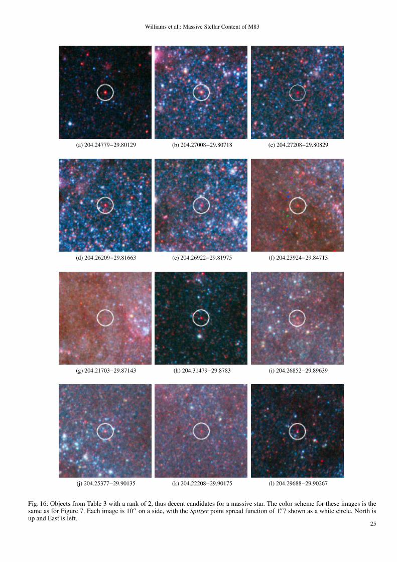
Fig. 16: Objects from Table 3 with a rank of 2, thus decent candidates for a massive star. The color scheme for these images is thesame as for Figure 7. Each image is 10′′ on a side, with the Spitzer point spread function of 1.′′7 shown as a white circle. North isup and East is left.

25


(a) 204.23015−29.91522 (b) 204.23495−29.9153 (c) 204.21763−29.92694

(d) 204.28307−29.84473 (e) 204.30836−29.84737 (f) 204.25821−29.85125

(g) 204.31955−29.85543 (h) 204.31419−29.85995 (i) 204.23301−29.87065

(j) 204.20346−29.87159

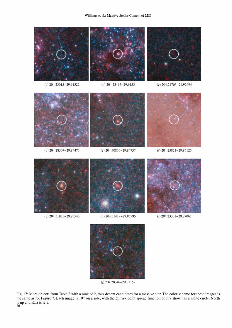
Fig. 17: More objects from Table 3 with a rank of 2, thus decent candidates for a massive star. The color scheme for these images isthe same as for Figure 7. Each image is 10′′ on a side, with the Spitzer point spread function of 1.′′7 shown as a white circle. Northis up and East is left.26


(a) 204.28665−29.81637 (b) 204.28041−29.81667 (c) 204.28956−29.81703

(d) 204.25643−29.81915 (e) 204.26219−29.81984 (f) 204.26318−29.81985

(g) 204.27432−29.82038 (h) 204.24071−29.83772 (i) 204.26684−29.84411

(j) 204.29662−29.85237 (k) 204.23938−29.86178 (l) 204.27568−29.87186

Fig. 18: Objects from Table 3 with a rank of 3, thus not good candidates for a massive star. The color scheme for these images is thesame as for Figure 7. Each image is 10′′ on a side, with the Spitzer point spread function of 1.′′7 shown as a white circle. North isup and East is left.

27


(a) 204.30318−29.87883 (b) 204.27873−29.88957 (c) 204.22592−29.89037

(d) 204.24112−29.89317 (e) 204.24035−29.89695 (f) 204.25784−29.89818

(g) 204.20358−29.89852 (h) 204.28941−29.9027 (i) 204.27719−29.91304

(j) 204.29721−29.91526 (k) 204.29463−29.91608 (l) 204.27929−29.91728

Fig. 19: More objects from Table 3 with a rank of 3, thus not good candidates for a massive star. The color scheme for these imagesis the same as for Figure 7. Each image is 10′′ on a side, with the Spitzer point spread function of 1.′′7 shown as a white circle. Northis up and East is left.28


(a) 204.26318−29.92358 (b) 204.26171−29.9246 (c) 204.24593−29.92507

(d) 204.23161−29.89652

Fig. 20: More objects from Table 3 with a rank of 3, thus not good candidates for a massive star. The color scheme for these imagesis the same as for Figure 7. Each image is 10′′ on a side, with the Spitzer point spread function of 1.′′7 shown as a white circle. Northis up and East is left.

29


(a) 204.26152−29.81385 (b) 204.22893−29.8338 (c) 204.23292−29.83584

(d) 204.24608−29.83645 (e) 204.24191−29.83685 (f) 204.30085−29.85674

(g) 204.24128−29.87485 (h) 204.20519−29.89473 (i) 204.3009−29.90026

(j) 204.28363−29.90948 (k) 204.23725−29.9241 (l) 204.23186−29.92541

Fig. 21: Objects from Table 3 with a rank of 4, thus very poor candidates for a massive star. The color scheme for these images isthe same as for Figure 7. Each image is 10′′ on a side, with the Spitzer point spread function of 1.′′7 shown as a white circle. Northis up and East is left.30


(a) 204.2652−29.81649 (b) 204.23216−29.84833 (c) 204.21583−29.85924

(d) 204.27851−29.8657 (e) 204.20375−29.89278 (f) 204.25955−29.92432

Fig. 22: More objects from Table 3 with a rank of 4, thus very poor candidates for a massive star. The color scheme for these imagesis the same as for Figure 7. Each image is 10′′ on a side, with the Spitzer point spread function of 1.′′7 shown as a white circle. Northis up and East is left.

31


(a) 204.25765−29.81874 (b) 204.27278−29.86357 (c) 204.29479−29.90216

(d) 204.22135−29.90849

Fig. 23: Objects from Table 3 with a rank of 5, thus extremely poor candidates for a massive star. The color scheme for these imagesis the same as for Figure 7. Each image is 10′′ on a side, with the Spitzer point spread function of 1.′′7 shown as a white circle. Northis up and East is left.

32

the infrared massive stellar content of m83 - arxiv · williams et al.: massive stellar content of...

Documents