the influence of thermal evolution in the magnetic protection of terrestrial planets
TRANSCRIPT

The Astrophysical Journal, 770:23 (23pp), 2013 June 10 doi:10.1088/0004-637X/770/1/23C© 2013. The American Astronomical Society. All rights reserved. Printed in the U.S.A.
THE INFLUENCE OF THERMAL EVOLUTION IN THE MAGNETIC PROTECTIONOF TERRESTRIAL PLANETS
Jorge I. Zuluaga1, Sebastian Bustamante1, Pablo A. Cuartas1, and Jaime H. Hoyos21 Instituto de Fısica-FCEN, Universidad de Antioquia, Calle 67 No. 53-108, Medellın, Colombia; [email protected],
[email protected], [email protected] Departamento de Ciencias Basicas, Universidad de Medellın, Carrera 87 No. 30-65, Medellın, Colombia; [email protected]
Received 2012 March 20; accepted 2013 April 10; published 2013 May 21
ABSTRACT
Magnetic protection of potentially habitable planets plays a central role in determining their actual habitability and/or the chances of detecting atmospheric biosignatures. Here we develop a thermal evolution model of potentiallyhabitable Earth-like planets and super-Earths (SEs). Using up-to-date dynamo-scaling laws, we predict the propertiesof core dynamo magnetic fields and study the influence of thermal evolution on their properties. The level ofmagnetic protection of tidally locked and unlocked planets is estimated by combining simplified models of theplanetary magnetosphere and a phenomenological description of the stellar wind. Thermal evolution introduces astrong dependence of magnetic protection on planetary mass and rotation rate. Tidally locked terrestrial planetswith an Earth-like composition would have early dayside magnetopause distances between 1.5 and 4.0 Rp, largerthan previously estimated. Unlocked planets with periods of rotation ∼1 day are protected by magnetospheresextending between 3 and 8 Rp. Our results are robust in comparison with variations in planetary bulk compositionand uncertainties in other critical model parameters. For illustration purposes, the thermal evolution and magneticprotection of the potentially habitable SEs GL 581d, GJ 667Cc, and HD 40307g were also studied. Assuming anEarth-like composition, we found that the dynamos of these planets are already extinct or close to being shut down.While GL 581d is the best protected, the protection of HD 40307g cannot be reliably estimated. GJ 667Cc, evenunder optimistic conditions, seems to be severely exposed to the stellar wind, and, under the conditions of ourmodel, has probably suffered massive atmospheric losses.
Key words: planetary systems – planets and satellites: magnetic fields – planets and satellites: physical evolution –planet–star interactions
Online-only material: color figures
1. INTRODUCTION
The discovery of extrasolar habitable planets is one of themost ambitious challenges in exoplanetary research. At thetime of writing, there are almost 861 confirmed exoplanets3
including 61 classified as Earth-like planets (EPs, M ∼ 1 M⊕)and super-Earths (SEs, M ∼ 1–10 M⊕; Valencia et al. 2006,hereafter VAL06). Among these low-mass planets, there arethree confirmed SEs, GJ 667Cc (Bonfils et al. 2011), GL 581d(Udry et al. 2007; Mayor et al. 2009), and HD 40307g (Tuomiet al. 2012), and tens of Kepler candidates (Borucki et al. 2011;Batalha et al. 2012) that are close to or inside the habitable zone(HZ) of their host stars (see, e.g., Selsis et al. 2007; Pepe et al.2011; Kaltenegger et al. 2011). If we include the possibilitythat giant exoplanets could harbor habitable exomoons, thenumber of the potentially habitable planetary environmentsalready discovered beyond the solar system could be raisedto several tens (Underwood et al. 2003; Kaltenegger 2010).Moreover, the existence of a plethora of other terrestrial planets(TPs) and exomoons in the Galaxy is rapidly gaining evidence(Borucki et al. 2011; Catanzarite & Shao 2011; Bonfils et al.2011; Kipping et al. 2012), and the chances that a large numberof potentially habitable extrasolar bodies could be discovered inthe near future are very large.
The question of which properties a planetary environmentneed in order to allow the appearance, evolution, and diversifi-cation of life has been extensively studied (for recent reviews,
3 For updates, please refer to http://exoplanet.eu
see Lammer et al. 2009 and Kasting 2010). Two basic and com-plementary physical conditions must be fulfilled: the presence ofan atmosphere and the existence of liquid water on the surface(Kasting et al. 1993). However, the fulfillment of these basicconditions depends on many complex and diverse endogenousand exogenous factors (for a comprehensive enumeration ofthese factors, see, e.g., Ward & Brownlee 2000 or Lammer et al.2010).
The existence and long-term stability of an intense planetarymagnetic field (PMF) is one of these relevant factors (see, e.g.,Grießmeier et al. 2010 and references therein). It has beenshown that a strong enough PMF could protect the atmosphereof potentially habitable planets, especially its valuable contentof water and other volatiles, against the erosive action of thestellar wind (Lammer et al. 2003, 2007; Khodachenko et al.2007; Chaufray et al. 2007). Planetary magnetospheres also actas shields against the potentially harmful effects that the stellarhigh energy particles and galactic cosmic rays (CR) producein the life forms evolving on the planetary surface (see, e.g.,Grießmeier et al. 2005). Even in the case that life could arise andevolve on unmagnetized planets, the detection of atmosphericbiosignatures would also be affected by a higher flux of highenergy particles including CR, especially if the planet is closeto very active M-dwarfs (dM; Grenfell et al. 2007; Segura et al.2010).
It has recently been predicted that most of the TPs in ourGalaxy could be found around dM stars (Boss 2006; Mayor &Udry 2008; Scalo et al. 2007; Rauer et al. 2011; Bonfils et al.2011). Actually, ∼20% of the presently confirmed SEs belong
1

The Astrophysical Journal, 770:23 (23pp), 2013 June 10 Zuluaga et al.
to planetary systems around stars of this type. Planets in the HZof low-mass stars (M� � 0.6 M�) would be tidally locked (Joshiet al. 1997; Heller et al. 2011), a condition that poses seriouslimitations to their potential habitability (see, e.g., Kite et al.2011 and references therein). Tidally locked planets inside theHZ of dMs have periods in the range of 5–100 days, a conditionthat has commonly been associated with the almost completelack of a protective magnetic field (Grießmeier et al. 2004).However, the relation between rotation and PMF properties,which is critical at assessing the magnetic protection of slowlyrotating planets, is more complex than previously thought. Inparticular, a detailed knowledge of the thermal evolution of theplanet is required to predict not only the intensity but also theregime (dipolar or multipolar) of the PMF for a given planetarymass and rotation rate (Zuluaga & Cuartas 2012).
Although several authors have extensively studied the pro-tection that intrinsic PMF would provide to extrasolar planets(Grießmeier et al. 2005; Khodachenko et al. 2007; Lammer et al.2007; Grießmeier et al. 2009, 2010), all have disregarded theinfluence that thermal evolution has in the evolution of planetarymagnetic properties. They have also used outdated dynamo scal-ing laws that have been recently revised (see Christensen 2010and references therein). The role of rotation in determining thePMF properties that is critical in assessing the case of tidallylocked planets has also been overlooked (Zuluaga & Cuartas2012).
We develop a comprehensive model for the evolution ofthe magnetic protection of potentially habitable TPs aroundGKM main-sequence stars. To achieve this goal, we integratein a single framework a parameterized thermal evolution modelbased on the most recent advances in the field (Gaidos et al.2010; Tachinami et al. 2011; Stamenkovic et al. 2012), up-to-date dynamo scaling laws (Christensen 2010; Zuluaga & Cuartas2012), and phenomenological models for the evolution of thestellar wind and planet–star magnetic interaction (Grießmeieret al. 2010). Our model is aimed at (1) understanding theinfluence of thermal evolution in the magnetic protection ofTPs, (2) assessing the role of low rotation periods in theevolution of the magnetic protection of tidally locked habitableplanets, (3) placing more realistic constraints on the magneticproperties of potentially habitable TPs suitable for future studiesof atmospheric mass loss or the CR effect on the atmosphericchemistry or on life itself, and (4) estimating by the first timethe magnetic properties of SEs already discovered in the HZ oftheir host stars.
Our work is a step forward in the understanding of planetarymagnetic protection because it combines in a single model theevolution of the magnetic properties of the planet and hence itsdependence on planetary mass and composition and the roleof the planet–star interaction into determining the resultinglevel of magnetic protection. Previous models of the former(thermal evolution and intrinsic magnetic properties) did notconsider the interaction of the PMF with the evolving stellarwind which is finally the factor that determines the actual levelof planetary magnetic protection. On the other hand, previousattempts to study the planet–star interaction overlooked the non-trivial dependence of intrinsic magnetic properties on planetarythermal evolution and hence on planetary mass and rotation rate.Additionally, and for the first time, we are attempting here tocalculate the magnetic properties of the potentially habitableSEs already discovered, GJ 667Cc, Gl 581d, and HD 40307g.
This paper is organized as follows. Section 2 is aimed atintroducing the properties of planetary magnetospheres we
should estimate in order to evaluate the level of magneticprotection of a potentially habitable TP. Once those propertiesare expressed in terms of two basic physical quantities, theplanetary magnetic dipole moment and the pressure of thestellar wind, we proceed to describe how those quantities canbe estimated by modeling the thermal evolution of the planet(Section 3), scaling the dynamo properties from the planetarythermal and rotational properties (Section 4), and modelingthe interaction between the star and the planet (Section 5). InSection 6, we apply our model to evaluate the level of magneticprotection of hypothetical potentially habitable TPs as well asthe habitable SEs already discovered. We also present the resultsof a numerical analysis aimed at evaluating the sensitivity of ourmodel to uncertainties in the composition of the planet and toother critical parameters of the model. In Section 7, we discussthe limitations of our model, present an example of the way inwhich our results could be applied to estimate the mass-loss ratefrom already and yet to be discovered potentially habitable TPs,and discuss the observational prospects to validate or improvethe model. Finally, a summary and several conclusions drawnfrom this research are presented in Section 8.
2. CRITICAL PROPERTIES OF AN EVOLVINGMAGNETOSPHERE
The interaction between the PMF, the interplanetary mag-netic field (IMF), and the stellar wind creates a magnetic cavityaround the planet known as the magnetosphere. Although mag-netospheres are very complex systems, their global propertiesare continuous functions of only two physical variables (Siscoe& Christopher 1975): the magnetic dipole moment of the planet,M, and the dynamic pressure of the stellar wind, Psw. Dipolemoment is defined in the multipolar expansion of the magneticfield strength:
Bp(r) = μ0M4πr3
+ O(
1
r4
), (1)
where Bp(r) is the angular-averaged PMF strength measured ata distance r from the planet center and μ0 = 4π × 10−7 H m−1
is the vacuum permeability. In the rest of the paper, we will dropoff the higher order terms in 1/r (multipolar terms) and focuson the dipolar component of the field B
dipp which is explicitly
given by the first term of the right side in Equation (1).The dynamic pressure of the stellar wind is given by
Psw = mnv2eff + 2nkBT . (2)
where m and n are the typical mass of a wind particle (mostlyprotons) and its number density, respectively. Here, veff =(v2
sw + v2p)1/2 is the effective velocity of the stellar wind as
measured in the reference frame of the planet whose orbitalvelocity is vp. T is the local temperature of the wind plasma andkB = 1.38 × 10⁻²³ J K−1 is the Boltzmann constant.
There are three basic properties of planetary magnetosphereswe are interested in: (1) the maximum magnetopause field in-tensity Bmp, which is a proxy of the flux of high energy par-ticles entering into the magnetospheric cavity; (2) the standoffor stagnation radius, RS, a measure of the size of the daysidemagnetosphere; and (3) the area of the polar cap Apc that mea-sures the total area of the planetary atmosphere exposed to openfield lines through which particles can escape to interplanetaryspace. The value of these quantities provides information about
2

The Astrophysical Journal, 770:23 (23pp), 2013 June 10 Zuluaga et al.
the level of exposure that a habitable planet has to the erosiveeffects of stellar wind and the potentially harmful effects ofthe CR.
The maximum value of the magnetopause field intensity Bmpis estimated from the balance between the magnetic pressurePmp = B2
mp/(2μ0) and the dynamic stellar wind pressure Psw(Equation (2)),
Bmp = (2μ0)1/2P 1/2sw . (3)
Here, we are assuming that the pressure exerted by theplasma inside the magnetospheric cavity is negligible (see thediscussion below).
Although magnetopause fields arise from very complexprocesses (Chapman–Ferraro and other complex currents at themagnetosphere boundary), in simplified models Bmp is assumedto be proportional to the PMF intensity Bp as measured at thesubstellar point r = RS (Mead 1964; Voigt 1995),
Bmp = 2f0Bp(r = RS) ≈(
f0μ0
2π
) √2MR−3
S . (4)
f0 is a numerical enhancement factor of the order of one that canbe estimated numerically. We are assuming here that the dipolarcomponent of the intrinsic field (the first term on the right-handside of Equation (1)) dominates at magnetopause distances evenin slightly dipolar PMF.
Combining Equations (3) and (4) we estimate the standoffdistance:
RS =(
μ0f20
8π2
)1/6
M1/3P −1/6sw
which can be expressed in terms of the present dipole momentof the Earth M⊕ = 7.768×10²² A m2 and the average dynamicpressure of the solar wind as measured at the orbit of our planetPsw� = 2.24 × 10⁻⁹ Pa (Stacey 1992; Grießmeier et al. 2005):
RS
R⊕= 9.75
(MM⊕
)1/3 (Psw
Psw�
)−1/6
. (5)
It is important to stress that the value of RS estimated withEquation (5) assumes a negligible value of the plasma pressureinside the magnetospheric cavity. This approximation is valid ifat least one of these conditions is fulfilled: (1) the PMF is veryintense, (2) the dynamic pressure of the stellar wind is small,or (3) the planetary atmosphere is not too bloated by the XUVradiation. In the case when any of these conditions are fulfilled,we will refer to RS as given by Equation (5) as the magneticstandoff distance which is an underestimation of the actual sizeof the magnetosphere.
Last, but not least, we are interested in evaluating the areaof the polar cap. This is the region in the magnetosphere wheremagnetic field lines could be open into the interplanetary spaceor to the magnetotail region. Siscoe & Chen (1975) have shownthat the area of the polar cap Apc scales with dipole moment anddynamic pressure as
Apc
4πR2p
= 4.63%
(MM⊕
)−1/3 (Psw
Psw�
)1/6
. (6)
Here, we have normalized the polar cap area with the totalarea of the atmosphere 4πR2
p, and assumed the atmosphere hasa scale height much smaller than planetary radius Rp.
In order to model the evolution of these three key magneto-sphere properties we need to estimate the surface dipolar compo-nent of the PMF B
dipp (Rp) (from which we can obtain the dipole
moment M), the average number density n, velocity veff , andtemperature T of the stellar wind (which are required to predictthe dynamic pressure Psw). These quantities depend in generalon time and also on different planetary and stellar properties. Inthe following sections, we describe our model for the calculationof the evolving values of these fundamental quantities.
3. THERMAL AND DYNAMO EVOLUTION
We assume here that the main source of a global PMF inTPs is the action of a dynamo powered by convection in aliquid metallic core (Stevenson 1983, 2003). This assumptionis reasonable since the Moon and all rocky planets in the solarsystem, regardless of their different origins and compositions,seem to presently have, or to previously had, an iron coredynamo (see, e.g., Stevenson 2010). Other potential sourcesof PMFs, such as body currents induced by the stellar magneticfield or dynamo action in a mantle of ice, water, or magma, arenot considered here but left for future research.
The properties and evolution of a core dynamo will depend onthe internal structure and thermal history of the planet. Thermalevolution of TPs, specially the Earth itself, has been studied fordecades (for a recent review, see Nimmo 2009). A diversity ofthermal evolution models for planets larger than the Earth haverecently appeared in literature (Papuc & Davies 2008; Gaidoset al. 2010; Tachinami et al. 2011; Driscoll & Olson 2011;Stamenkovic et al. 2011). But the lack of observational evidenceagainst which we can compare the predictions of these modelshas left too much room for uncertainties, especially regardingmantle rheology, core composition, and thermodynamic prop-erties. Albeit these fundamental limitations, a global picture ofthe thermal history of SEs has started to arise. Here, we followthe lines of Labrosse (2003) and Gaidos et al. (2010) develop-ing a parameterized thermal evolution model which combinesa simplified model of the interior structure and a parameterizeddescription of the core and mantle rheology.
Our model includes several distinctive characteristics incomparison to previous ones. The most important one is an up-to-date treatment of mantle rheology. For that purpose, we usetwo different formulae to compute the viscosity of the upper andlower mantles. By lower mantle, we understand here the regionof the mantle close to the core–mantle boundary (CMB). Thisis the hottest part of the mantle. The upper mantle is the outercold part of this layer. It is customary to describe both regionswith the same rheology albeit their very different mineralogicalcompositions. Additionally, thermal and density profiles in themantle follow the same prescription as in the core. We alsouse a different ansatz to assign initial values to lower mantletemperature and to the temperature contrast across the CMB,two of the most uncertain quantities in thermal evolution models.Using our ansatz, we avoid assigning arbitrary initial values tothese critical parameters but more importantly we are able tofind a unified method to set the value of these temperatures inplanets with very different masses. It is also important to notethat in other models these temperatures were set by hand or weretreated as free parameters in the model.
Four key properties should be predicted by any thermalevolution model in order to calculate the magnetic properties of aplanet: (1) the total available convective power Qconv, providingthe energy required for magnetic field amplification through
3

The Astrophysical Journal, 770:23 (23pp), 2013 June 10 Zuluaga et al.
dynamo action; (2) the radius of the solid inner core Ric andfrom there the height D ≈ Rc − Ric of the convecting shellwhere the dynamo action takes place (Rc is the radius of thecore); (3) the time of inner core formation tic; and (4) the totaldynamo lifetime tdyn.
In order to calculate these quantities, we solve simply pa-rameterized energy and entropy equations of balance describingthe flux of heat and entropy in the planetary core and mantle.As stated before, our model is based on the interior structuremodel by VAL06 and in thermal evolution models previouslydeveloped by Schubert et al. (1979), Stevenson (1983), Nimmo& Stevenson (2000), Labrosse et al. (2001), Labrosse (2003),Gubbins et al. (2003, 2004), Aubert et al. (2009), Gaidos et al.(2010), and Stamenkovic et al. (2011). For a detailed descriptionof the fundamental physics behind the thermal evolution modeldeveloped here, please refer to these earlier studies.
3.1. Interior Structure
Our one-dimensional model for the interior assumes a planetmade by two well-differentiated chemically and mineralogicallyhomogeneous shells: a rocky mantle made out of olivine andperovskite and a core made by iron plus other light elements.
The mechanical conditions inside the planet (pressure P,density ρ, and gravitational field g) are computed by simul-taneously solving the continuity, Adams–Williamson, and hy-drostatic equilibrium equations (Equations (1)–(4) in VAL06).For all planetary masses, we assume boundary conditions,ρ(r = Rp) = 4000 kg m−3 and P (r = Rp) = 0 Pa. Foreach planetary mass and core mass fraction CMF = Mcore/Mp,we use an RK4 integrator and a shooting method to consistentlycompute the core Rc and planetary radius Rp.
For the sake of simplicity, we do not include in the in-terior model the two- or even three-layered structure of themantle. Instead, we assume a mantle completely made ofperovskite–postperovskite (ppv). This is the reason why we takeρ(r = Rp) = 4000 kg m−3 instead of the more realistic value of3000 kg m−3. With a single layer and a realistic surface density,our model is able to reproduce the present interior properties ofthe Earth.
In all cases, we use the Vinet equation of state instead of thecommonly used third-order Birch–Murnaghan equation (BM3).It is well known that the BM3 follows from a finite strain expan-sion and does not accurately predict the properties of the materialfor the typical pressures found in SEs, i.e., 100–1000 GPa forMp = 1–10 M⊕ (VAL06; Tachinami et al. 2011). We have ig-nored thermal corrections to the adiabatic compressibility, i.e.,KS(ρ, T ) ≈ KS(ρ, 300 K)+ΔKs(T ) (VAL06). This assumptionallows us to decouple at runtime the CPU intensive calculationof the thermal profile from the mechanical structure at each timestep in the thermal evolution integration.
Although we have ignored the “first-order” effect of the tem-perature in the mechanical structure, we have taken into account“second-order” effects produced by phase transitions inside themantle and core. Using the initial temperature profile insidethe mantle, we calculate the radius of transition from olivine toperovskite (neglecting the effect of an intermediate layer of wad-sleyite). For that purpose, we use the reduced pressure functionΠ (Christensen 1985; Weinstein 1992; Valencia et al. 2007). Forsimplicity, the position of the transition layer is assumed to beconstant during the whole thermal evolution of the planet. Wehave verified that this assumption does not significantly changethe mechanical properties inside the planet, at least not at a levelaffecting the thermal evolution itself.
Inside the core, we continuously update the radius of thetransition from solid to liquid iron (see below). For that purpose,we use the thermal profile computed at the previous time step.To avoid a continuous update of the mechanical structure, weassume in all the cases that during the transition from solidto liquid the density of iron changes by a constant factorΔρ = (ρs − ρl)/ρl . Here, the reference density of the solid ρs
(when applied) is computed using the Vinet equation evaluatedat a point in the very center of the planet.
Table 1 enumerates the relevant physical parameters of theinterior structure and thermal evolution model.
3.2. Core Thermal Evolution
In order to compute the thermal evolution of the core, wesolve the equations of energy and entropy balance (Labrosseet al. 2001; Nimmo 2009):
Qc = Qs + fi(Qg + Ql) (7)
Φ = El + fi(Es + Eg) − Ek. (8)
Here, Qc is the total heat flowing through the CMB and Φis the total entropy dissipated in the core. Es and Qs are theentropy and heat released by the secular cooling, Eg and Qg arethe contribution to entropy and heat due to the redistribution ofgravitational potential when light elements are released at theliquid–solid interface (buoyant energy), El and Ql are the entropyand heat released by the phase transition (latent heat), and Ek isa term accounting for the sink of entropy due to the conductionof heat along the core. We have avoided the terms coming fromradioactive and pressure heating because their contribution isnegligible at the typical conditions inside SEs (Nimmo 2009).As long as the buoyant and latent entropy and heat are onlypresent when a solid inner core exists, we have introduced aboolean variable fi that turns on these terms when the conditionfor the solidification of the inner core arises.
The terms in the energy and entropy balance are a functionof the time derivative of the temperature profile ∂T (r, t)/∂t (fordetailed expressions of these terms, see Table 1 in Nimmo 2009).As an example, the secular heat and entropy are given by
Qs = −∫
ρcp
∂T (r, t)
∂tdV,
Es = −∫
ρcp
[1
Tc(t)− 1
T (r, t)
]∂T (r, t)
∂tdV . (9)
Here, cp is the specific heat of the core alloy and Tc is thetemperature at the CMB. If we assume that the temperatureprofile of the core does not change during the thermal evolution,we can write temperature as T (r, t) = fc(r)Tc(t). Here, fc(r) isthe core temperature radial profile that we will assume adiabatic(see below). It should be noted again that Tc(t) = T (r = Rc, t).
With this assumption the energy balance equation (7) can bewritten as a first-order differential equation on Tc:
Qc = Mc[Cs + fi(Cg + Cl)]dTc
dt, (10)
where Mc is the total mass of the core and Cs, Cg, and Cl arecore bulk heat capacities which can be expressed as volumetricintegrals of the radial profile fc(r). In this equation, the totalheat Qc is intrinsically a function of Tc and should be computedindependently (see below).
4
The Astrophysical Journal, 770:23 (23pp), 2013 June 10 Zuluaga et al.
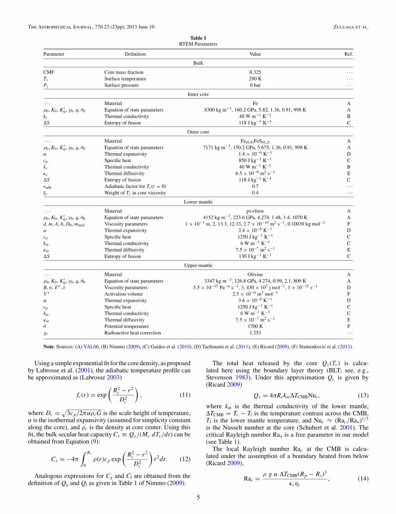
Table 1RTEM Parameters
Parameter Definition Value Ref.
Bulk
CMF Core mass fraction 0.325 · · ·Ts Surface temperature 290 K · · ·Ps Surface pressure 0 bar · · ·
Inner core
· · · Material Fe Aρ0, K0, K ′
0, γ0, q, θ0 Equation of state parameters 8300 kg m−3, 160.2 GPa, 5.82, 1.36, 0.91, 998 K Akc Thermal conductivity 40 W m−1 K−1 BΔS Entropy of fusion 118 J kg−1 K−1 C
Outer core
· · · Material Fe(0,8)FeS(0,2) Aρ0, K0, K ′
0, γ0, q, θ0 Equation of state parameters 7171 kg m−3, 150.2 GPa, 5.675, 1.36, 0.91, 998 K Aα Thermal expansivity 1.4 × 10⁻⁶ K−1 Dcp Specific heat 850 J kg−1 K−1 Ckc Thermal conductivity 40 W m−1 K−1 Bκc Thermal diffusivity 6.5 × 10⁻⁶ m2 s−1 EΔS Entropy of fusion 118 J kg−1 K−1 Cεadb Adiabatic factor for Tc(t = 0) 0.7 · · ·ξc Weight of Tc in core viscosity 0.4 · · ·
Lower mantle
· · · Material pv+fmw Aρ0, K0, K ′
0, γ0, q, θ0 Equation of state parameters 4152 kg m−3, 223.6 GPa, 4.274, 1.48, 1.4, 1070 K Ad, m, A, b, D0, mmol Viscosity parameters 1 × 10⁻³ m, 2, 13.3, 12.33, 2.7 × 10⁻¹⁰ m2 s−1, 0.10039 kg mol−1 Fα Thermal expansivity 2.4 × 10⁻⁶ K−1 Dcp Specific heat 1250 J kg−1 K−1 Ckm Thermal conductivity 6 W m−1 K−1 Cκm Thermal diffusivity 7.5 × 10⁻⁷ m2 s−1 EΔS Entropy of fusion 130 J kg−1 K−1 C
Upper mantle
· · · Material Olivine Aρ0, K0, K ′
0, γ0, q, θ0 Equation of state parameters 3347 kg m−3, 126.8 GPa, 4.274, 0.99, 2.1, 809 K AB, n, E∗, ε Viscosity parameters 3.5 × 10⁻¹⁵ Pa−n s−1, 3, 430 × 103 j mol−1, 1 × 10⁻¹⁵ s−1 DV ∗ Activation volume 2.5 × 10⁻⁶ m3 mol−1 Fα Thermal expansivity 3.6 × 10⁻⁶ K−1 Dcp Specific heat 1250 J kg−1 K−1 Ckm Thermal conductivity 6 W m−1 K−1 Cκm Thermal diffusivity 7.5 × 10⁻⁷ m2 s−1 Eθ Potential temperature 1700 K Fχr Radioactive heat correction 1.253 · · ·
Note. Sources: (A) VAL06, (B) Nimmo (2009), (C) Gaidos et al. (2010), (D) Tachinami et al. (2011), (E) Ricard (2009), (F) Stamenkovic et al. (2011).
Using a simple exponential fit for the core density, as proposedby Labrosse et al. (2001), the adiabatic temperature profile canbe approximated as (Labrosse 2003)
fc(r) = exp
(R2
c − r2
D2c
), (11)
where Dc = √3cp/2παρcG is the scale height of temperature,
α is the isothermal expansivity (assumed for simplicity constantalong the core), and ρc is the density at core center. Using thisfit, the bulk secular heat capacity Cs ≡ Qs/(Mc dTc/dt) can beobtained from Equation (9):
Cs = −4π
∫ Rc
0ρ(r)cp exp
(R2
c − r2
D2c
)r2dr. (12)
Analogous expressions for Cg and Cl are obtained from thedefinition of Qg and Ql as given in Table 1 of Nimmo (2009).
The total heat released by the core Qc(Tc) is calcu-lated here using the boundary layer theory (BLT; see, e.g.,Stevenson 1983). Under this approximation Qc is given by(Ricard 2009)
Qc = 4πRckmΔTCMBNuc, (13)
where km is the thermal conductivity of the lower mantle,ΔTCMB = Tc − Tl is the temperature contrast across the CMB,Tl is the lower mantle temperature, and Nuc ≈ (Rac/Ra∗)1/3
is the Nusselt number at the core (Schubert et al. 2001). Thecritical Rayleigh number Ra∗ is a free parameter in our model(see Table 1).
The local Rayleigh number Rac at the CMB is calcu-lated under the assumption of a boundary heated from below(Ricard 2009),
Rac = ρ g α ΔTCMB(Rp − Rc)3
κcηc
, (14)
5

The Astrophysical Journal, 770:23 (23pp), 2013 June 10 Zuluaga et al.
where g is the gravitational field and κc the thermal diffusivityat the CMB. The value of the dynamic viscosity ηc, which isstrongly dependent on temperature, could be suitably computedusing the so-called film temperature (see Manga et al. 2001and references therein). This temperature could be computedin general as a weighted average of the temperatures at theboundaries,
Tηc = ξcTc + (1 − ξc)Tl, (15)
where the weighting coefficient ξc is a free parameter whosevalue is chosen in order to reproduce the thermal properties ofthe Earth (see Table 1).
To model the formation and evolution of the solid inner core,we need to compare at each time the temperature profile with theiron solidus. We use here the Lindemann law as parameterizedby VAL06:
∂ log τ
∂ log ρ= 2 [γ − δ(ρ)] . (16)
Here, δ(ρ) ≈ 1/3 and γ is an effective Gruneisen parameterthat, for simplicity, is assumed to be constant. To integrate thisequation, we use the numerical density profile provided by theinterior model and the reference values ρ0 = 8300 kg m−3 (pureiron) and τ0 = 1808 K.
The central temperature T (r = 0, t) and the solidus atthat point τ (r = 0) are compared at each time step. WhenT (0, tic) ≈ τ (0) (tic is the time of inner core formation) we turnon the buoyant and latent heat terms in Equations (7) and (8),i.e., set fi = 1, and continue the integration including theseterms. The radius of the inner core at times t > tic is obtainedby solving the equation proposed by Nimmo (2009) and furtherdeveloped by Gaidos et al. (2010),
dRic
dt= − D2
c
2Ric(Δ − 1)
1
Tc
dTc
dt. (17)
Here, Δ is the ratio between the gradient of the solidus(Equation (16)) and the actual temperature gradient Tc(t)fc(r)as measured at Ric(t).
When the core cools down below a given level the outer layersstart to stratificate. Here, we model the effect of stratificationby correcting the radius and temperature of the core followingthe prescription by Gaidos et al. (2010). When stratified theeffective radius of the core is reduced to R� (Equation (27)in Gaidos et al. 2010) and the temperature at the core surfaceis increase to T� (Equation (28) in Gaidos et al. 2010). Thestratification of the core reduces the height of the convectiveshell which leads to a reduction of the Coriolis force potentiallyenhancing the intensity of the dynamo-generated magnetic field.
The estimation of the dynamo properties requires the compu-tation of the available convective power Qconv. Qconv is calculatedhere assuming that most of the dissipation occurs at the top ofthe core. Under this assumption,
Qconv(t) ≈ Φ(t)Tc(t), (18)
where the total entropy Φ is computed from the entropy balance(Equation (8)) using the solution for the temperature profileTc(t)fc(r).
When Φ(t) becomes negative, i.e., El + Es + Eg < Ek inEquation (8), Qconv also becomes negative and convection is nolonger efficient to transport energy across the outer core. Underthis condition, the dynamo is shut down. The integration stopswhen this condition is fulfilled at a time we label as the dynamolifetime tdyn.
3.3. Mantle Thermal Evolution
One of the novel features of our thermal evolution model isthat we treat mantle thermal evolution with a similar formalismas that described before for the metallic core.
The energy balance in the mantle can be written as
Qm = χrQr + Qs + Qc. (19)
Here, Qm is the total heat flowing out through the surfaceboundary (SB), Qr is the heat produced in the decay ofradioactive nuclides inside the mantle, Qs is the secular heat,and Qc is the heat coming from the core (Equation (13)).
We use here the standard expressions and parameters forthe radioactive energy production as given by Kite et al.(2009). However, in order to correct for the non-homogeneousdistribution of radioactive elements in the mantle, we introduce amultiplicative correction factor χr . Here, we adopt χr = 1.253that fits the Earth properties well. We have verified that thethermal evolution is not too sensitive to χr and have assumedthe same value for all planetary masses.
The secular heat in the mantle is computed using an expres-sion analogous to Equation (9). As in the case of the core, we as-sume that the temperature radial profile does not change duringthe thermal evolution. Under this assumption, the temperatureprofile in the mantle can be also written as T (r, t) = Tm(t)fm(r).In this case, Tm(t) = T (r = Rp, t) is the temperature just belowthe SB layer (see Figure 1).
Assuming an adiabatical temperature profile in the mantle,we can also write:
fm(r) = exp
(R2
p − r2
D2m
),
in analogy to the core temperature profile (Equation (11)).In this expression, Dm is the temperature scale height for themantle which is related to the density scale height Lm throughD2
m = L2m/γ (Labrosse 2003). In our simplified model, we take
the values of the density at the boundaries of the mantle andanalytically obtain an estimate for Lm and hence for Dm.
The energy balance in the mantle is balanced when weindependently calculate the heat Qm at the SB as a functionof Tm. In this case, whether or not mobile lids are present playsan important role in determining the efficiency with which theplanet gets rid of the heat coming from the mantle. In the mobilelid regime, we assume that the outer layer is fully convectiveand use the BLT approximation to calculate Qm,
QMLm = 4πR2
pkmΔTmNum
Rp − Rc
, (20)
where ΔTm = Tm − Ts is the temperature contrast across theSB and Ts is the surface temperature. Since we are studying thethermal evolution of habitable planets, in all cases we assumeTs = 290 K. Planetary interior structures and thermal evolutionare not too sensitive to surface temperature. We have verifiedthat the results are nearly the same for the surface temperaturein the range of 250–370 K. In the mobile lid regime, Num obeys
6

The Astrophysical Journal, 770:23 (23pp), 2013 June 10 Zuluaga et al.
Figure 1. Schematic representation of the planetary interior. In the schematic slice, we depict the main quantities used here to describe the thermal evolution of theplanets. The temperature profile depicted below the slice does not use real data. Distances and sizes are not represented with the right scale.
(A color version of this figure is available in the online journal.)
the same relationship with the critical Rayleigh number as inthe core. In this case, however, we compute the local Rayleighnumber under the assumption of material heated from inside(Gaidos et al. 2010),
Ram = αgρ2H (Rp − Rc)5
kmκmηm
, (21)
where H = (Qr + Qc)/Mm is the density of heat inside themantle, km and κm are the thermal conductivity and diffusivity,respectively, and ηm is the upper mantle viscosity.
In the stagnant lid regime, the SB provides a rigid boundaryfor the heat flux. In this case, we adopt the approximation usedby Nimmo & Stevenson (2000):
QSLm = 4πR2
p
km
2
(ρgα
κmηm
)1/3
Γ−4/3. (22)
Here, Γ ≡ −∂ ln ηm/∂Tm measures the viscosity dependenceon temperature evaluated at the average mantle pressure.
With all these elements at hand the energy balance atEquation (19) is finally transformed into an ordinary differentialequation for the upper mantle temperature Tm(t),
Qm = χrQr + Qc + Cm
dTm
dt, (23)
where Cm is the bulk heat capacity of the upper mantle which iscalculated with an expression analogous to Equation (12).
3.4. Initial Conditions
In order to solve the coupled differential equations (10), (17),and (23), we need to choose a proper set of initial conditions.
The initial value of the upper mantle temperature is chosenusing the prescription by Stamenkovic et al. (2011). Accordingto this prescription, Tm(t = 0) is computed by integrating
the pressure-dependent adiabatic equation up to the averagepressure inside the mantle 〈Pm〉,
Tm(t = 0) = θ exp
(∫ 〈Pm〉
0
γ0
Ks(P ′)dP′
). (24)
Here, θ = 1700 K is a potential temperature which is assumed tobe the same for all planetary masses (Stamenkovic et al. 2011).Using Tm(t = 0) and the adiabatic temperature profile, we canobtain the initial lower mantle temperature Tl(t = 0).
The initial value of the core temperature Tc(t = 0) is oneof the most uncertain parameters in thermal evolution models.Although its actual value or its dependence on the formationhistory and planetary mass is not known, it is reasonable to startthe integration of a simplified thermal evolution model whenthe core temperature is of the same order as the melting pointfor MgSiO3 at the lower mantle pressure. A small arbitrarytemperature contrast against this reference value (Gaidos et al.2010; Tachinami et al. 2011) or more complicated mass-dependent assumptions (Papuc & Davies 2008) have been usedin previous models to set the initial core temperature. We usehere a simple prescription that agrees reasonably well withprevious attempts and provides a unified expression that couldbe used consistently for all planetary masses.
According to our prescription, the temperature contrast acrossthe CMB is assumed to be proportional to the temperaturecontrast across the whole mantle, i.e., ΔTCMB = εadbΔTadb =εadb(Tm − Tl). We have found that the thermal evolution prop-erties of Earth are reproduced when we set εadb = 0.7.
Using this prescription, the initial core temperature is finallycalculated using
Tc(t = 0) = Tl + εadbΔTadb. (25)
We have observed that the value of the Tc(t = 0) obtainedwith this prescription is very close to the perovskite melt-ing temperature at the CMB for all the planetary masses
7

The Astrophysical Journal, 770:23 (23pp), 2013 June 10 Zuluaga et al.
studied here. This result shows that although our criterion isnot particularly better physically rooted than those used in pre-vious models, it still relies in just one free parameter, i.e., theratio of mantle and CMB contrasts εadb.
3.5. Rheological Model
One of the most controversial aspects and probably thelargest source of uncertainties in thermal evolution models isthe calculation of the rheological properties of silicates and ironat high pressures and temperatures. A detailed discussion onthis important topic is beyond the scope of this paper. An up-to-date discussion and analysis of the dependence on pressureand temperature of viscosity in SEs and its influence in thermalevolution can be found in the recent works by Tachinami et al.(2011) and Stamenkovic et al. (2011).
We use here two different models to calculate viscosityunder different ranges of temperatures and pressures. For thehigh pressures and temperatures of the lower mantle, we use aNabarro–Herring model (Yamazaki & Karato 2001),
ηNH(P, T ) = Rgdm
D0AmmolTρ(P, T ) exp
(b Tmelt(P )
T
). (26)
Here, Rg = 8.31 J mol−1 K−1 is the gas constant, d is the grainsize, m is the growing exponent, A and b are free parameters,D0 is the pre-exponential diffusion coefficient, mmol is the molardensity of perovskite, and Tmelt(P ) is the melting temperatureof perovskite that can be computed with the empirical fit:
Tmelt(P ) =4∑
i=0
ai · P i.
All the parameters used in the viscosity model, including theexpansion coefficients ai in the melting temperature formula,were taken from the recent work by Stamenkovic et al. (2011).The Nabarro–Herring formula allows us to compute ηc =ηNH(Tηc), where Tηc is the film temperature computed usingthe average in Equation (15).
The upper mantle has a completely different mineralogy andit is under the influence of lower pressures and temperatures.Although previous works have used the same model and parame-ters to calculate viscosity across the whole mantle (Stamenkovicet al. 2011, for example, use the perovskite viscosity parame-ters also in the olivine upper mantle), we have found here thatusing a different rheological model in the upper and lower man-tles avoids under- and overestimation, respectively, of the valueof viscosity that could have a significant effect on the thermalevolution.
In the upper mantle, we find that using an Arrhenius-typemodel leads to better estimates of viscosity than that obtainedusing the Nabarro–Herring model. In the upper mantle, theNabarro–Herring formula (which is best suited to describe thedependence on viscosity at high pressures and temperatures)leads to huge underestimations of viscosity in that region. In thecase of the Earth, this underestimation produces values of thetotal mantle too high compared to that observed in our planetmaking impossible to fit the thermal evolution of a simulatedEarth.
For the Arrhenius-type formula, we use the same parameter-ization given by Tachinami et al. (2011):
ηA(P, T ) = 1
2
[1
B1/nexp
(E∗ + PV ∗
nRgT
)]ε(1−n)/n, (27)
Figure 2. Thermal evolution of TPs with an Earth-like composition (CMF =0.325) using the RTEM (see Table 1). Upper panel: convective power flux Qconv(see Equation (18)). Middle panel: radius of the inner core Ric. Lower panel:time of inner core formation (blue squares) and dynamo lifetime (red circles).In the RTEM, the metallic core is liquid at t = 0 for all planetary masses.Planets with a mass Mp < Mcrit = 2.0 M⊕ develop a solid inner core beforethe shutdown of the dynamo while the core of more massive planets remainsliquid at least until the dynamo shutdown.
(A color version of this figure is available in the online journal.)
where ε is the strain rate, n is the creep index, B is theBarger coefficient, and E∗ and V ∗ are the activation energyand volume. The values assumed here for these parameters arethe same as that given in Table 4 of Tachinami et al. (2011)except for the activation volume whose value we assume hereV ∗ = 2.5×10⁻⁶ m3 mol−1. Using the formula in Equation (27),the upper mantle viscosity is computed as ηm = ηA(〈Pm〉, Tm).
A summary of the parameters used by our interior and thermalevolution models is presented in Table 1. The values listedin Column 3 define what we will call the reference thermalevolution model (RTEM). These reference values have beenmostly obtained by fitting the present interior properties ofthe Earth and the global features of its thermal, dynamo, andmagnetic field evolution (time of inner core formation andpresent values of Ric, Qm and surface magnetic field intensity).For the stagnant lid case, we use, as suggested by Gaidos et al.(2010), the values of the parameters that globally reproduce thepresent thermal and magnetic properties of Venus.
Figure 2 shows the results of applying the RTEM to a set ofhypothetical TPs in the mass range Mp = 0.5–6 M⊕.
8

The Astrophysical Journal, 770:23 (23pp), 2013 June 10 Zuluaga et al.
4. PLANETARY MAGNETIC FIELD
In recent years, improved numerical experiments have con-strained the full set of possible scaling laws used to predict theproperties of planetary and stellar convection-driven dynamos(see Christensen 2010 and references therein). It has been foundin a wide range of physical conditions that the global proper-ties of a planetary dynamo can be expressed in terms of simplepower-law functions of the total convective power Qconv and thesize of the convective region.
One of the most important results of power-based scalinglaws is the fact that the volume-averaged magnetic field intensityB2
rms = (1/V )∫
B2dV does not depend on the rotation rate ofthe planet (Equation (6) in Zuluaga & Cuartas 2012),
Brms ≈ CBrms μ1/20 ρc
1/6(D/V )1/3Q1/3conv. (28)
Here, CBrms is a fitting constant obtained from numericaldynamo experiments and its value is different in the case ofdipolar-dominated dynamos, C
dipBrms = 0.24, and multipolar
dynamos, CmulBrms = 0.18. ρc, D = R� − Ric, and V =
4π (R3� − R3
ic)/3 are the average density, height, and volumeof the convective shell.
The dipolar field intensity at the planetary surface, andhence the dipole moment of the PMF, can be estimated if wehave information about the power spectrum of the magneticfield at the core surface. Although we cannot predict therelative contribution of each mode to the total core fieldstrength, numerical dynamos exhibit an interesting property:there is a scalable dimensionless quantity, the local Rossbynumber Ro∗
l , that could be used to distinguish dipolar-dominatedfrom multipolar dynamos. The scaling relation for Ro∗
l is(Equation (5) in Zuluaga & Cuartas 2012)
Ro∗l = CRol
ρc−1/6R−2/3
c D−1/3V −1/2Q1/2convP
7/6. (29)
Here, CRol= 0.67 is a fitting constant and P is the period of
rotation. It has been found that dipolar-dominated fields arisesystematically when dynamos have Ro∗
l < 0.1. Multipolar fieldsarise in dynamos with values of the local Rossby number closeto and larger than this critical value. From Equation (29), wesee that in general fast rotating dynamos (low P) have dipolar-dominated core fields while slowly rotating ones (large P)produce multipolar fields and hence fields with a much lowerdipole moment.
It is important to stress that the almost independence of Brmson rotation rate, together with the role that rotation has in thedetermination of the core field regime, implies that even veryslowly rotating planets could have a magnetic energy budget ofcomparable sized than rapidly rotating planets with similar sizeand thermal histories. In the former case, the magnetic energywill be redistributed among other multipolar modes renderingthe core field more complex in space and probably also in time.Together all these facts introduce a non-trivial dependence ofdipole moment on rotation rate very different from that obtainedwith the traditional scaling laws used in previous works (see,e.g., Grießmeier et al. 2004; Khodachenko et al. 2007). Here,we emphasize a property that was also previously overlooked.Multipolar-dominated dynamos produce magnetic fields thatdecay more rapidly with distance than dipolar fields and so it isexpected that a planet with a multipolar magnetic field will beless protected than those having strongly dipolar fields.
Using the value of Brms and Ro∗l , we can compute the
maximum dipolar component of the field at the core surface.
For this purpose, we use an upper bound to the dipolarityfraction fdip (the ratio of the dipolar component to the totalfield strength at core surface). Dipolar-dominated dynamos bydefinition have fdip � f max
dip = 1.0. The case of reversing dipolarand multipolar dynamos is more complex. Numerical dynamoexperiments show that multipolar dynamos have Ro∗
l � 0.1and fdip � f max
dip = 0.35. However, to avoid inhomogeneitiesin the transition region around Ro∗
l ≈ 0.1, we calculate amaximum dipolarity fraction through a “soft step function,”f max
dip = α+β/{exp[(Ro∗l −0.1)/δ]+1} with α, β, and δ numerical
constants that fit the envelope of the numerical dynamo data (seethe upper panel of Figure 1 in Zuluaga & Cuartas 2012).
To connect this ratio to the volumetric-averaged magneticfield Brms, we use the volumetric dipolarity fraction bdip that isfound, as shown by numerical experiments, conveniently relatedto the maximum value of fdip through Equation (12) in Zuluaga& Cuartas (2012),
bmindip = cbdipf
maxdip
−11/10, (30)
where cbdip ≈ 2.5 is again a fitting constant. It is important tonotice here that the exponent 11/10 is the ratio of the smallestintegers close to the numerical value of the fitting exponent (seeFigure 1 in Zuluaga & Cuartas 2012). We use this conventionfollowing Olson & Christensen (2006).
Finally by combining Equations (28)–(30), we can computean upper bound to the dipolar component of the field at theCMB:
Bdipc � 1
bmindip
Brms = f maxdip
11/10
cbdipBrms. (31)
The surface dipolar field strength is estimated using
Bdipp (Rp) = Bdip
c
(Rp
Rc
)3
(32)
and finally the total dipole moment is calculated usingEquation (1) for r = Rp.
It should be emphasized that the surface magnetic fieldintensity determined using Equation (32) overestimates thePMF dipolar component. The actual field could be much morecomplex spatially and the dipolar component could be lower. Asa consequence, our model can only predict the maximum levelof protection that a given planet could have from a dynamo-generated intrinsic PMF.
The results of applying the RTEM to calculate the propertiesof the magnetic field of TPs in the mass range 0.5–4.0 M⊕using the scaling laws in Equations (28), (29), and (31) aresummarized in Figures 3 and 4. In Figure 3, we show the localRossby number, the maximum dipolar field intensity, and thedipole moment as a function of time computed for planetswith different masses and two different periods of rotation(P = 1 day and P = 2 days). This figure shows the effect thatrotation has on the evolution of dynamo geometry and hence inthe maximum attainable dipolar field intensity at the planetarysurface. In Figure 4, we have summarized in mass–period (M–P)diagrams (Zuluaga & Cuartas 2012) the evolution of the dipolemoment for planets with long-lived dynamos. We see that forperiods lower than one day and larger than five to seven daysthe dipole moment is nearly independent of rotation. Slowlyrotating planets have a non-negligible dipole moment that issystematically larger for more massive planets.
9

The Astrophysical Journal, 770:23 (23pp), 2013 June 10 Zuluaga et al.
Figure 3. PMF properties predicted using the RTEM and Equations (28), (29),and (31) for TPs 0.5–4.0 M⊕. We plot the local Rossby number (lower panel),the maximum surface dipole field (middle panel), and the maximum dipolemoment (upper panel). We included the present values of the geodynamo (“⊕”symbol) and three measurements of paleomagnetic intensities (error bars) at 3.2and 3.4 Gyr ago (Tarduno et al. 2010). We compare the magnetic properties fortwo periods of rotation, one day (solid curves), and two days (dashed curves).The effect of a larger period of rotation is more significant at early times in thecase of massive planets (Mp � 2 M⊕) and at late times for lower mass planets.
(A color version of this figure is available in the online journal.)
5. PLANET–STAR INTERACTION
The PMF properties constrained using the thermal evolutionmodel and the dynamo-scaling laws are not enough to evaluatethe level of magnetic protection of a potentially habitable TP. Wealso need to estimate the magnetosphere and stellar properties(stellar wind and luminosity) as a function of time in order toproperly assess the level of star–planet interaction.
Since the model developed in previous sections providesonly the maximum intensity of the PMF, we will be interestedhere in constraining the magnetosphere and stellar propertiesfrom below, i.e., to find the lower level of “stellar aggression”for a given star–planet configuration. Combining the upperbounds of PMF properties and the lower bounds for thestar–planet interaction will produce an overestimation of theoverall magnetic protection of a planet. If, using this model, agiven star–planet configuration is not suitable to provide enoughmagnetic protection to the planet, the actual case should be muchworse. If, on the other hand, our upper limit approach predicts ahigh level of magnetic protection, the actual case could still bethat of an unprotected planet. Therefore, our model is capableof predicting which planets will be unprotected but less able topredict which ones will actually be protected.
5.1. The Habitable Zone (HZ) and Tidally Locking Limits
The surface temperature and hence “first-order” habitabilityof a planet depends on three basic factors: (1) the fundamental
Figure 4. Mass–period (M–P) diagrams of the dipole moment for long-livedplanetary dynamos using the RTEM. Three regimes are identified (Zuluaga& Cuartas 2012): rapid rotating planets (P � 1 day), dipole moments arelarge and almost independent of rotation rate; slowly rotating planets (1 day �P � 5 day), dipole moments are intermediate in value and highly dependenton rotation rate; and very slowly rotating planets (P � 5–10 days), small butnon-negligible rotation-independent dipole moments. For (Mp < 2 M⊕), theshape of the dipole-moment contours is determined by tic.
(A color version of this figure is available in the online journal.)
properties of the star (luminosity L�, effective temperature T�,and radius R�), (2) the average star–planet distance (distanceto the HZ), and (3) the commensurability of planetary rotationand orbital period (tidal locking). These properties should beproperly modeled in order to assess the degree of star–planetinteraction which is critical for determining the magneticprotection.
The basic properties of main-sequence stars of differentmasses and metallicities have been studied for decades andare becoming critical for assessing the actual properties ofnewly discovered exoplanets. The case of low-mass main-sequence stars (GKM) are particularly important for providingthe properties of the stars with the highest potential to harborhabitable planets with evolved and diverse biospheres.
In this work, we will use the theoretical results of Baraffe et al.(1998, hereafter BAR98) that predict the evolution of different
10

The Astrophysical Journal, 770:23 (23pp), 2013 June 10 Zuluaga et al.
Figure 5. HZ limits corresponding to the conservative criteria of recent Venus and early Mars according to the updated limits estimated by Kopparapu et al. (2013).Stellar properties are computed at τ = 3 Gyr using the models by Baraffe et al. (1998). Planets at distances below the dashed line would be tidally locked before0.7 Gyr (Peale 1977). The location of Earth, Venus, and the potentially habitable extrasolar system planets GL 581d, GJ 667Cc, and HD 40307g are also included.
(A color version of this figure is available in the online journal.)
Table 2Properties of the SEs Already Discovered Inside the HZ of Their Host Stars
Planet Mp Rp a Po e S-type M� Age Tid. Locked Refs.(M⊕) (R⊕) (AU) (days) (M�) (Gyr)
Earth 1.0 1.0 1.0 365.25 0.016 G2V 1.0 4.56 No · · ·Venus 0.814 0.949 0.723 224.7 0.007 G2V 1.0 4.56 Probably · · ·GJ 667Cc 4.545 1.5∗ 0.123 28.155 <0.27 M1.25V 0.37 >2.0 Yes (1)GL 581d 6.038 1.6∗ 0.22 66.64 0.25 M3V 0.31 4.3–8.0 Yes (2), (3)HD 40307g 7.1 1.7∗ 0.6 197.8 0.29 K2.5V 0.77 4.5 No (4)
Notes. For reference purposes, the properties of Venus and the Earth are also included. Values of radii marked with an “∗” are unknown andwere estimated using the mass–radius relation for planets with the same composition as the Earth, i.e., Rp = R⊕(Mp/M⊕)0.27 (VAL06).References. (1) Bonfils et al. 2011; (2) Udry et al. 2007; (3) Mayor et al. 2009; (4) Tuomi et al. 2012.
metallicities main-sequence GKM stars. We have chosen fromthat model those results corresponding to the case of solarmetallicity stars. We have disregarded the fact that the basicstellar properties actually evolve during the critical period wheremagnetic protection will be evaluated, i.e., t = 0.5–3 Gyr. Tobe consistent with the purpose of estimating upper limits ofmagnetic protection, we took the stellar properties as providedby the model at the highest end of the time interval, i.e.,t = 3 Gyr. Since luminosity increases with time in GKM stars,this assumption guarantees the largest distance of the HZ andhence the lowest effects of the stellar insolation and the stellarwind.
In order to estimate the HZ limits, we use the recently updatedvalues calculated by Kopparapu et al. (2013). In particular, weuse the interpolation formula in Equation (2) and coefficients inTable (2) to compute the most conservative limits of recentVenus and early Mars. The limits calculated for the stellarproperties assumed here are depicted in Figure 5.
The orbital and rotational properties of planets at close-inorbits are strongly affected by gravitational and tidal interactionswith the host star. Tidal torque dampens the primordial rotationand axis tilt leaving the planet in a final resonant equilibriumwhere the period of rotation P becomes commensurable with
the orbital period Po,
P : Po = n : 2. (33)
Here, n is an integer larger than or equal to 2. The value of nis determined by multiple dynamic factors, the most importantbeing the orbital planetary eccentricity (Leconte et al. 2010;Ferraz-Mello et al. 2008; Heller et al. 2011). In the solar system,the tidal interaction between the Sun and Mercury has trappedthe planet in a 3:2 resonance. In the case of GL 581d, detaileddynamic models predict a resonant 2:1 equilibrium state (Helleret al. 2011), i.e., the rotation period of the planet is a half of itsorbital period.
Although in general estimating the time required for the“tidal erosion” is very hard given the large uncertainties in thekey physical parameters involved (see Heller et al. 2011 for adetailed discussion), the maximum distance atid at which a solidplanet in a circular orbit becomes tidally locked before a giventime t can be roughly estimated by (Peale 1977)
atid(t) = 0.5 AU
[(M�/M�)2Pprim
Q
]1/6
t1/6. (34)
11

The Astrophysical Journal, 770:23 (23pp), 2013 June 10 Zuluaga et al.
Here, the primordial period of rotation Pprim should beexpressed in hours, t in Gyr, and Q is the dimensionlessdissipation function. For the purposes of this work, we assumea primordial period of rotation Pprim = 17 hr (Varga et al. 1998;Denis et al. 2011) and a dissipation function Q ≈ 100 (Henninget al. 2009; Heller et al. 2011).
In Figure 5, we summarize the properties of solar metallicityGKM main-sequence stars provided by the BAR98 model andthe corresponding limits of the HZ and tidal locking maximumdistance. The properties of the host stars of the potentiallyhabitable SEs already discovered, GL 581d, GJ 667Cc, andHD 40307g, are also highlighted in this figure.
5.2. Stellar Wind
The stellar wind and CRs pose the highest risks for amagnetically unprotected potentially habitable TP. The dynamicpressure of the wind is able to obliterate an exposed atmosphere,especially during the early phase of stellar evolution (Lammeret al. 2003), and energetic stellar CRs could pose a serious riskto any form of surface life directly exposed to them (Grießmeieret al. 2005).
The last step in order to estimate the magnetospheric prop-erties and hence the level of magnetic protection is predictingthe stellar wind properties for different stellar masses and as afunction of planetary distance and time.
There are two simple models used to describe the spatial struc-ture and dynamics of the stellar wind: the pure hydrodynamicalmodel originally developed by Parker (1958) that describes thewind as a non-magnetized, isothermal, and axially symmetricflux of particles (hereafter Parker’s model), and the more de-tailed albeit simpler magneto-hydrodynamic model originallydeveloped by Weber & Davis (1967) that takes into account theeffects of stellar rotation and treats the wind as a magnetizedplasma.
It has been shown that Parker’s model reliably describes theproperties of the stellar winds in the case of stars with periodsof rotation of the same order as the present solar value, i.e.,P ∼ 30 days (Preusse et al. 2005). However, for rapidly rotatingstars, i.e., young stars and/or active dM stars, the isothermalmodel underestimates the stellar wind properties by almost afactor of two (Preusse et al. 2005). For the purposes of scaling theproperties of the planetary magnetospheres (Equations (3)–(6)),an underestimation of the stellar wind dynamic pressure of thatsize will give us values of the key magnetospheric properties thatwill be off by 10%–40% of the values given by more detailedmodels. Magnetopause fields that have the largest uncertaintieswill be underestimated by ∼40%, while standoff distances andpolar cap areas will be, respectively, under- and overestimatedby just ∼10%.
According to Parker’s model, the stellar wind average particlevelocity v at distance d from the host star is obtained by solvingParker’s wind equation (Parker 1958):
u2 − log u = 4 log ρ +4
ρ− 3, (35)
where u = v/vc and ρ = d/dc are the velocity and dis-tance normalized with respect to vc = √
kBT /m and dc =GM�m/(4kBT ) which are, respectively, the local sound velocityand the critical distance where the stellar wind becomes sub-sonic. T is the temperature of the plasma which, in the isothermalcase, is assumed to be constant at all distances and equal to thetemperature of the stellar corona. T is the only free parametercontrolling the velocity profile of the stellar wind.
The number density n(d) is calculated from the velocity usingthe continuity equation:
n(d) = M�
4πd2v(d)m. (36)
Here, M� is the stellar mass-loss rate, which is a freeparameter in the model.
To calculate the evolution of the stellar wind, we need a wayto estimate the evolution of the coronal temperature T and themass-loss rate M�.
Using observational estimates of the stellar mass-loss rate(Wood et al. 2002) and theoretical models for the evolution of thestellar wind velocity (Newkirk 1980), Grießmeier et al. (2004)and Lammer et al. (2004) developed semiempirical formulaeto calculate the evolution of the long-term-averaged numberdensity and velocity of the stellar wind for main-sequence starsat a given reference distance (1 AU):
v1 AU(t) = v0
(1 +
t
τ
)αv
(37)
n1 AU(t) = n0
(1 +
t
τ
)αn
. (38)
Here, αv = −0.43, αn = −1.86 ± 0.6, and τ = 25.6 Myr(Grießmeier et al. 2009). The parameters v0 = 3971 km s−1
and n0 = 1.04 × 10¹¹ m−3 are estimated from the present long-term averages of the solar wind as measured at the distanceof the Earth n(4.6 Gyr, 1 AU, 1 M�) = 6.59 × 10⁶ m−3 andv(4.6 Gyr, 1 AU, 1 M�) = 425 km s−1 (Schwenn 1990).
Using these formulae, Grießmeier et al. (2007a) devised aclever way to estimate consistently T (t) and M�(t) in Parker’smodel and hence we are able predict the stellar wind propertiesas a function of d and t. For the sake of completeness, wesummarize this procedure here. For further details, see Section2.4 in Grießmeier et al. (2007a).
For a stellar mass M� and time t, the velocity of the stellarwind at d = 1 AU, v1 AU, is calculated using Equation (37).Replacing this velocity in Parker’s wind equation for d = 1 AU,we numerically find the temperature of the corona T (t). Thisparameter is enough to provide the whole velocity profilev(t, d,M�) at time t. To compute the number density, we needthe mass-loss rate for this particular star and at this time. Usingthe velocity and number density calculated from Equations (37)and (38), the mass-loss rate for the Sun M� at time t andd = 1 AU can be obtained:
M�(t) = 4π (1 AU)2 m n1 AU(t)v1 AU(t). (39)
Assuming that the mass-loss rate scales simply with the stellarsurface area, i.e., M�(t) = M�(t)(R�/R�)2, the value of M� canfinally be estimated. Using v(t, d,M�) and M� in the continuityequation (36), the number density of the stellar wind n(t, d,M�)is finally obtained.
The value of the stellar wind dynamic pressurePdyn(t, d,M�) = m n(t, d,M�) v(t, d,M�)2 inside the HZ offour different stars as computed using the procedure describedpreviously is plotted in Figure 6.
It is important to stress here that for stellar ages t � 0.7 Gyrthe semiempirical formulae in Equations (37) and (38) arenot longer reliable (Grießmeier et al. 2007a). These equationsare based on the empirical relationship observed between theX-ray surface flux and the mass-loss rate M� (Wood et al.
12

The Astrophysical Journal, 770:23 (23pp), 2013 June 10 Zuluaga et al.
Figure 6. Evolution of the stellar wind dynamic pressure at the center of the HZ for a selected set of stellar masses. The reference average solar wind pressure isPSW� = 1.86 nPa. The dashed curves indicate the value of the stellar wind pressure at the inner and outer edges of the HZ around stars with 0.2 M� and 1.0 M�,respectively. The HZ limits where the pressure was calculated are assumed to be static and equal to those at τ = 3 Gyr. Stellar wind pressure at t < 0.7 Gyr computedwith the semiempirical model used in this work is too uncertain and was not plotted.
(A color version of this figure is available in the online journal.)
2002, 2005) which has been reliably obtained only for agest � 0.7 Gyr. However, Wood et al. (2005) have shown thatan extrapolation of the empirical relationship to earlier timesoverestimates the mass-loss rate by a factor of 10–100. Attimes t � 0.7 Gyr and over a given magnetic activity threshold,the stellar wind of main-sequence stars seems to be inhibited(Wood et al. 2005). Therefore, the limit placed by observationsat t ≈ 0.7 Gyr is not simply an observational constraint butcould mark the time where the early stellar wind also reachesa maximum (J. L. Linsky 2012, private communication). Thisfact suggests that at early times the effect of the stellar windon the planetary magnetosphere is much lower than normallyassumed. Hereafter, we will assume that intrinsic PMF is strongenough to protect the planet, at least until the maximum of thestellar wind is reached at t ≈ 0.7 Gyr, and focus on the stellarwind and magnetosphere properties for times larger than this.
6. RESULTS
Using the results of our RTEM, the power-based scaling lawsfor dynamo properties, and the properties of the stellar insolationand stellar wind pressure, we have calculated the magnetosphereproperties of EPs and SEs in the HZ of different main-sequencestars. We have performed these calculations for hypothetical TPsin the mass range 0.5–6 M⊕ and for the potentially habitableplanets already discovered GL 581d, GJ 667Cc, and HD 40307g(see Table 2). The case of the Earth and a habitable Venus havealso been studied for references purposes.
To include the effect of rotation in the properties of the PMF,we have assumed that planets in the HZ of late K and dM stars
(M < 0.7 M�) are tidally locked at times t < 0.7 Gyr (n =2 in Equation (33), see Figure 5). Planets around G and earlyK stars (M � 0.7 M�) will be assumed to have primordialperiods of rotation that we chose in the range 1–100 days aspredicted by models of planetary formation (Miguel & Brunini2010).
Figures 7 and 8 show the evolution of magnetosphere proper-ties for tidally locked and unlocked potentially habitable planets,respectively. In all cases, we have assumed that the planets arein the middle of the HZ of their host stars.
Even at early times, tidally locked planets of arbitrary masseshave non-negligible magnetosphere radii RS > 1.5 Rp. Previousestimates of the standoff distances for tidally locked planetsare much lower than the values reported here. As an example,Khodachenko et al. (2007) place the standoff distances wellbelow 2 Rp, even under mild stellar wind conditions (seeFigure 4 in their work) and independent of planetary mass andage. In contrast, our model predicts standoff distances for tidallylocked planets in the range of 2–6 Rp depending on planetarymass and stellar age. The differences between both predictionsarise mainly from the underestimation of the dipole moment forslowly rotating planets found in these works. Thermal evolutionand the dependency on planetary mass of the PMF properties areresponsible for the rest of the discrepancies in previous estimatesof the magnetosphere properties.
Though tidally locked planets seem to have larger magneto-spheres than previously expected, they still have large polar caps,a feature that was previously overlooked. As a consequence ofthis fact, well protected atmospheres, i.e., atmospheres that liewell inside of the magnetosphere cavity (hereafter magnetized
13

The Astrophysical Journal, 770:23 (23pp), 2013 June 10 Zuluaga et al.
Figure 7. Evolution of the magnetopause field (upper row), standoff distance (middle row), and polar cap area (lower row) of tidally locked (slow rotating) planetsaround late dK and dM stars. The rotation of each planet is assumed to be equal to the orbital period at the middle of the HZ (see the values in the rightmost verticalaxes). The value of the magnetosphere properties returned by the contour lines in these plots could be an under- or an overestimation of these properties according tothe position of a planet inside the HZ. In the case of GL 581d (GJ 667Cc), which is located in the outer (inner) edge of the HZ, the magnetopause field and polar caparea are overestimated (underestimated) while the standoff distance is underestimated (overestimated).
(A color version of this figure is available in the online journal.)
planets), could have more than 15% of their surface area ex-posed to open field lines where thermal and non-thermal pro-cesses could efficiently remove atmospheric gases. Moreover,our model predicts that these planets would have multipolarPMF which contributes to an increase of the atmospheric areaopen to the interplanetary and magnetotail regions (Siscoe &Crooker 1976). Then the exposition of magnetized planets toharmful external effects would be a complex function of thestandoff distance and the polar cap area.
Overall, magnetic protection improves with time. As the starevolves, the dynamic pressure of the stellar wind decreases morerapidly than the dipole moment (see Figures 4 and 6). As aconsequence, the standoff distance grows in time and the polarcap shrinks. However, with the reduction in time of the stellar
wind pressure, the magnetopause field is also reduced, whichcan affect the incoming flux of CR at late times.
The sinuous shape of the contour lines in the middle andlower rows is a byproduct of the inner core solidification inplanets with Mp < 2 M⊕. Critical boundaries between regionswith very different behaviors in the magnetosphere propertiesare observed at Mp ∼ 1.0 M⊕ and Mp ∼ 1.8 M⊕ in the middleand rightmost panels of the standoff radius and polar cap areacontours. Planets to the right of these boundaries still have acompletely liquid core and therefore produce weaker PMFs(lower standoff radius and larger polar cap areas). On the otherhand, the inner cores in planets to the left of the these boundarieshave already started to grow and therefore their PMFs arestronger.
14

The Astrophysical Journal, 770:23 (23pp), 2013 June 10 Zuluaga et al.
Figure 8. Same as Figure 7 but for unlocked (fast rotating) planets around early K and G stars (M� � 0.7). For all planets, we have assumed a constant period ofrotation P = 1 day.
(A color version of this figure is available in the online journal.)
Unlocked planets (Figure 8) are better protected than slowlyrotating tidally locked planets by developing extended magne-tospheres RS � 4 Rp and lower polar cap areas Apc � 10%. Itis interesting to note that in both cases and at times t ∼ 1 Gyr asmaller planetary mass implies a lower level of magnetic protec-tion (lower standoff distances and larger polar caps). This resultseems to contradict the idea that low-mass planets (Mp � 2) arebetter suited to develop intense and protective PMFs (Gaidoset al. 2010; Tachinami et al. 2011; Zuluaga & Cuartas 2012).To explain this contradiction, one should take into accountthat magnetic protection as defined in this work depends ondipole moment instead of surface magnetic field strength. Sincedipole moment scales as M ∼ BdipR
3p, more massive planets
will have a better chance of having large and protective dipolemoments.
It is interesting to compare the predicted values of themaximum dipole moment calculated here with the valuesroughly estimated in previous attempts (Grießmeier et al. 2005;Khodachenko et al. 2007; Lopez-Morales et al. 2011). On onehand, Khodachenko et al. (2007) estimate dipole moments fortidally locked planets in the range 0.022–0.15M⊕. These valueshave been systematically used in the literature to study differentaspects of planetary magnetic protection (see, e.g., Lammer et al.2010 and references therein). For the same type of planets, ourmodel predicts maximum dipole moments almost one order ofmagnitude larger (0.15–0.60 M⊕) with the largest differencesfound for the most massive planets (M � 4 M⊕). Thesedifferences arise from the fact that none of the scaling laws usedby Khodachenko et al. (2007) depend on the convective power.In our results, the dependency on power explains the differences
15
The Astrophysical Journal, 770:23 (23pp), 2013 June 10 Zuluaga et al.
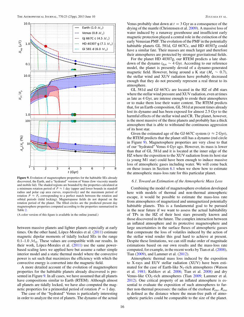
Figure 9. Evolution of magnetosphere properties for the habitable SEs alreadydiscovered, the Earth, and a “hydrated” version of Venus (low viscosity mantleand mobile lid). The shaded regions are bounded by the properties calculated ata minimum rotation period of P ≈ 1 day (upper and lower bounds in standoffradius and polar cap area curves, respectively) and the maximum period ofrotation P ≈ Po corresponding to a perfect match between the rotation andorbital periods (tidal locking). Magnetopause fields do not depend on therotation period of the planet. The filled circles are the predicted present daymagnetosphere properties computed according to the properties summarized inTable 2.
(A color version of this figure is available in the online journal.)
between massive planets and lighter planets especially at earlytimes. On the other hand, Lopez-Morales et al. (2011) estimatemagnetic dipolar moments of tidally locked SEs in the range0.1–1.0 M⊕. These values are compatible with our results. Intheir work, Lopez-Morales et al. (2011) use the same power-based scaling laws we applied here but assume a rather simpleinterior model and a static thermal model where the convectivepower is set such that maximizes the efficiency with which theconvective energy is converted into the magnetic field.
A more detailed account of the evolution of magnetosphereproperties for the habitable planets already discovered is pre-sented in Figure 9. In all cases, we have assumed that all planetshave compositions similar to Earth (RTEM). Although almostall planets are tidally locked, we have also computed the mag-netic properties for a primordial period of rotation P = 1 day.
The case of the “hydrated” Venus is particularly interestingin order to analyze the rest of planets. The dynamo of the actual
Venus probably shut down at t = 3 Gyr as a consequence of thedrying of the mantle (Christensen et al. 2009). A massive loss ofwater induced by a runaway greenhouse and insufficient earlymagnetic protection played a central role in the extinction of theearly Venusian PMF. The evolution of the PMF in the potentiallyhabitable planets GL 581d, GJ 667Cc, and HD 40307g couldhave a similar fate. Their masses are much larger and thereforetheir atmospheres are protected by stronger gravitational fields.
For the planet HD 40307g, our RTEM predicts a late shut-down of the dynamo tdyn ∼ 4 Gyr. According to our referencemodel, the planet is presently devoid of a dynamo-generatedmagnetic field. However, being around a K star (M� ∼ 0.7),the stellar wind and XUV radiation have probably decreasedenough that they do not presently represent a real threat to itsatmosphere.
GL 581d and GJ 667Cc are located in the HZ of dM starswhere the stellar wind pressure and XUV radiation, even at timesas late as 4 Gyr, are intense enough to erode their atmospheresor to make them lose their water content. The RTEM predictsthat, for an Earth-composition, GL 581d at present times alreadylost its dynamo and has been exposed for almost 2.5 Gyr to theharmful effects of the stellar wind and CR. The planet, however,is the most massive of the three planets and probably has a thickatmosphere that is able to withstand the continuous aggressionof its host star.
Given the estimated age of the GJ 667C system (t ≈ 2 Gyr),the RTEM predicts that the planet still has a dynamo (red circlein Figure 9). Magnetosphere properties are very close to thatof our “hydrated” Venus 4 Gyr ago. However, its mass is lowerthan that of GL 581d and it is located at the inner edge of theHZ where the exposition to the XUV radiation from its host star(a young M1 star) could have been enough to induce massiveloss of atmospheric gases including water. We will come backon these issues in Section 6.1 when we show how to estimatethe atmospheric mass-loss rate for this particular planet.
6.1. Toward an Estimation of the Atmospheric Mass Loss
Combining the model of magnetosphere evolution developedhere with models of thermal and non-thermal atmosphericescape, it would be possible to estimate the mass-loss ratefrom atmospheres of magnetized and unmagnetized potentiallyhabitable planets. This is a fundamental goal to be pursuedin the near future if we want to assess the actual habitabilityof TPs in the HZ of their host stars presently known andthose discovered in the future. The complex interaction betweenan inflated atmosphere and its protective magnetosphere andlarge uncertainties in the surface fluxes of atmospheric gassesthat compensate the loss of volatiles induced by the action ofthe stellar wind render this goal hard to achieve at present.Despite these limitations, we can still make order of magnitudeestimations based on our own results and the mass-loss ratecomputed, for example, in the recent works by Tian et al. (2008),Tian (2009), and Lammer et al. (2012).
Atmospheric thermal mass loss induced by the expositionto X-rays and EUV stellar radiation (XUV) have been esti-mated for the case of Earth-like N2-rich atmospheres (Watsonet al. 1981; Kulikov et al. 2006; Tian et al. 2008) and dryVenus-like CO2-rich atmospheres (Tian 2009; Lammer et al.2012). One critical property of an inflated atmosphere is es-sential to evaluate the exposition of such atmospheres to fur-ther non-thermal processes: the radius of the exobase Rexo. Rexois defined as the distance where the mean-free path of atmo-spheric particles could be comparable to the size of the planet.
16

The Astrophysical Journal, 770:23 (23pp), 2013 June 10 Zuluaga et al.
When the radius of the exobase is comparable to or larger thanthe magnetic standoff distance RS, we will say that the planet isunmagnetized. Under these conditions, the gases escaping fromthe exosphere will be picked up by the stellar wind and lostto the interplanetary space. On the other hand, if the exobase iswell inside the magnetosphere (which is the case of the Earth to-day) atmospheric gasses escaping thermally from the exospherecould stay trapped by the magnetic field forming a plasmas-phere. Planets under this condition will be magnetically pro-tected and the mass-loss rate is expected to be much lower thanfor unmagnetized planets.
Using the conservative estimation of the X and EUV lumi-nosities of main-sequence stars given by Garces et al. (2011),we have estimated the XUV flux at the top of the atmospheresof GL 581d, GJ 667Cc, and HD 40307g during the first crit-ical gigayear of planetary evolution. The planet that receivedthe minimum amount of XUV radiation is HD 40307g withFXUV = 10–35 PEL (1 PEL = 0.64 erg cm−2 s−1 is the presentEarth value; Judge et al. 2003; Guinan et al. 2009). GL 581d wasexposed in the first gigayear to a flux of FXUV = 150–250 PELwhile GJ 667Cc received the maximum amount of XUV radia-tion among them, FXUV = 450–800 PEL.
Using the recent results by Tian (2009) that computed theexosphere properties of massive SEs, i.e., Mp � 6 M⊕, subjectto different XUV fluxes, we can estimate the exosphere radiusand mass-loss rate for our three habitable SEs. Actually, sincethe Tian (2009) results are only available for planets with aminimum mass of Mp = 6 M⊕, a qualitative extrapolation ofthe results for 10, 7, and 6 M⊕ (see Figures 4 and 6 in his paper)shows that exobase radius and mass-loss rates are larger for lessmassive planets. This is particularly useful for trying to applythe Tian’s results to GJ 667Cc Mp ≈ 4.5 M⊕ and other lessmassive potentially habitable planets. In these cases, we willuse the results by Tian (2009) to calculate a lower bound of theexobase radius and mass-loss rates.
Using the estimated XUV flux for HD 40307g (Mp ≈ 7 M⊕)and assuming an initial CO2-rich atmosphere, Tian’s resultspredict that the exosphere of the planet and hence its mass-lossrate was low enough to avoid a significant early erosion of itsatmosphere (see Figures 4 and 6 in his paper). This is true at leastduring the first 1–2 Gyr during which our magnetic protectionmodel predicts that the planet was enshrouded by a protectivemagnetosphere (see Figure 9). After dynamo shutdown, theatmosphere of HD 40307g has been exposed to the direct actionof the stellar wind. Assuming a stellar age of 4.5 Gyr (Tuomiet al. 2012), this effect has eroded the atmosphere for 3–4 Gyr.During this unmagnetized phase, the atmospheric mass-loss ratecan be simply estimated as M ≈ αmnveff (Zendejas et al. 2010)where α is the so-called entrainment efficiency and m, n, andveff are the mass, number density, and effective velocity of thestellar wind as measured at planetary distance (see Equation (2)).Using a entrainment efficiency α ∼ 0.3 (which is appropriate,for example, to describe the mass loss of the Venus atmosphere),we find that the total mass loss during the unmagnetized phaseis less than 1% of a conservative estimate of the total volatilecontent of the planet (Tian 2009). Although our model providesonly upper limits to magnetic protection and the planet couldhave, for example, a lighter nitrogen-rich atmosphere which ismore prone to XUV-induced mass losses (Watson et al. 1981;Kulikov et al. 2006; Tian et al. 2008), this preliminary estimationsuggests that HD 40307g probably still preserves a dense enoughatmosphere that is able to sustain surface liquid water and henceto be actually habitable.
The case of GL 581d (Mp ≈ 6 M⊕) is quite different.Assuming that our estimations of the XUV flux are correct, theexosphere radius predicted by Tian (2009) should be close to theactual one. In this case at times t ∼ 1 Gyr, Rexo = 1.8–2.3 Rp.However, our reference magnetosphere model predicts for thisplanet magnetic standoff distances RS > 2.7 at all times. Weconclude that by using our estimations GL 581d could havebeen protected by its intrinsic magnetic field during the criticalearly phases of planetary evolution and probably has preservedthe critical volatiles in its atmosphere. Still, the uncertaintiesin the exosphere model or in the atmospheric composition andof course in the magnetic model developed here should leadto a different conclusion and further theoretical and probablyobservational investigation are required.
The most interesting case is that of GJ 667Cc (Mp ≈ 4.5 M⊕).The minimum exosphere radius predicted for this planet att ∼ 1 Gyr lies between 3.0 and 4.5 Rp while, according toour magnetosphere model, the magnetic standoff distance isRS < 3 Rp up to 2 Gyr. Since the exosphere radius shouldactually be larger than that predicted with the Tian (2009) modeland our magnetic model is actually optimistic, the chances thatthis planet was unprotected by its magnetic field in the criticalfirst gigayear are high. But exposition does not necessarily meana complete obliteration of the atmosphere (see, for example,the case of Venus). To evaluate the level of thermal and non-thermal obliteration of the atmosphere, we need to estimate theactual mass-loss rate. At the XUV fluxes estimated at the topof the atmosphere of this planet during the first gigayear, theminimum thermal mass-loss rate of carbon atoms from a CO2-rich atmosphere will be larger than 2–4 × 10¹⁰ atoms cm−2 s−1
(see Figure 6 in Tian 2009). We should recall that this is actuallythe value for a 6 M⊕ SE. For the actual mass of the planet,4.5 M⊕, the mass-loss rate could be even larger. Moreover, if, aspredicted here, the exosphere is directly exposed to the stellarwind, non-thermal processes can contribute to a larger increasein the mass loss from the planetary atmosphere. At the minimummass-loss rate, the exposed GJ 667Cc atmosphere could havelost more than ∼1046 atoms of carbon in just ∼100 Myr and inthe first gigayear the amount of carbon thermally lost to spacecould rise to ∼1047 atoms. If we scale up linearly with planetarymass, the total inventory of CO2 in the atmosphere, crust, andmantle of Venus, which is 2–3 × 1046 molecules (see Tian2009 and references therein), a 4.5 M⊕ planet will have a totalbudget of ∼1047 CO2 molecules. In summary, at the minimummass-loss rate and assuming a relatively rapid degassing of theplanet, Gj 667Cc could have lost its total inventory of carbonto interplanetary space in the first couple of gigayears. Evenassuming that large amounts of CO2 are still trapped in themantle and crust of the planet, its atmosphere should be rapidlyobliterated by the stellar wind. We speculate that GJ 667Cc is asort of “Venus-like” planet. Regardless the fact that the planetis inside the radiative HZ, it has lost its capacity to support lifevia a massive stellar-wind-induced loss of volatiles.
7. DISCUSSION
Applying simplified thermal evolution model and dynamoscaling laws to planets whose bulk properties are barely knownor even hypothetical, it is challenging and probably raises morequestions than it attempts to solve. Further observations of thepotentially habitable planets should be required to present theirprecise physical properties and to reliably model its interior andthermal evolution. Moreover, continued observational efforts
17
The Astrophysical Journal, 770:23 (23pp), 2013 June 10 Zuluaga et al.
to look for direct evidence or proxies of planetary magneto-spheres and any other signatures of magnetic protection, thoughchallenging, should also be attempted. Here, we discuss the as-sumptions on which our global model relies, its uncertaintiesas measured by the sensitivity of the model to changes in keyphysical parameters, and the missing pieces of information andpresent observational limitations to confirm or improve this andother models of planetary magnetic protection.
7.1. Model Assumptions
The strength of a physical model depends on the hypothesisand assumptions on which it relies. Apart from numerousalbeit very common assumptions, the magnetic protection modelpresented here depends on three major assumptions which wediscuss in the following paragraphs.
We have assumed that TPs always develop an initially metallicliquid core, irrespective of their composition and early formationhistory. This is not necessarily true. The formation of a metallicliquid core would depend on very complex processes and otherbarely known physical factors. It has been shown, for example,that under extreme water oxidation of iron the formation of ametallic core will be avoided (Elkins-Tanton & Seager 2008).In this case, silicate coreless planets will be formed. On theother hand, even if a planet is well differentiated the core couldbe solid from the beginning (see, e.g., VAL06). However, itshould be emphasized here that our model provides only thebest-case scenario of magnetic protection. Therefore, if, underthe assumption of having a liquid metallic core, a planet isfound to be lacking enough magnetic protection, the case whenthe planet is not well differentiated or when it never develops aliquid core will be even worse. In these cases, the conclusionsdrawn from our model will be unchanged.
The calculation of key magnetosphere properties relies onvery simplistic assumptions about the complex physics behindthe interaction between planetary and interplanetary magneticfields and stellar wind. In particular, standoff distances calcu-lated with Equation (5) assume a negligible plasma pressureinside the magnetosphere. This condition could be violated inplanets with very inflated atmospheres and/or at close-in or-bits. Under these extreme conditions, the magnetic standoffdistance given by Equation (5) could be a poor underestima-tion of the actual magnetopause distance. However, the weakdependence of standoff distances and polar cap areas of thestellar wind dynamic pressure offers some idea as to the actualrole that magnetospheric plasma pressure may pay in determin-ing the size of the magnetosphere. Adding a plasma pressureterm Ppl to the magnetic pressure Pmp in the left-hand side ofEquation (3) is equivalent to subtracting it from the stellar winddynamic pressure Psw in the right-hand side. An effective stellarwind pressure P ′
sw = Psw(1−Ppl/Psw) would replace the stellarwind term in the standoff distance definition (Equation (5)). As aresult a plasma pressure correcting factor (1−Ppl/Psw)−1/6 willmodify our estimated purely magnetic standoff distance. Evenin a case where the plasma was able to exert a pressure 50% ofthat of the stellar wind, the standoff distance will increase byonly 10%. On the other hand, in order to have a standoff distanceone order of magnitude larger than that estimated using Equa-tion (5), the plasma pressure inside the magnetosphere shouldamount to 99.999% of the total pressure. This is precisely whatan unmagnetized planet would look like. In summary, includingmore realistic condition in the definition of the magnetosphereboundary will not greatly modify our results.
A final but no less important assumption in our model is that ofquiet stellar wind conditions. We have only taken into accountaverage or quiet stellar wind conditions. We have completelyneglected the effects of large but transient conditions suchas those produced during coronal mass ejections (CMEs). Tomodel the effect that a steady flux/influx of CME plasma couldhave on close-in planets, we can modify the stellar wind pressureby maintaining the nominal velocity of the plasma but increasingthe number density of wind particles by a factor of two.4 Takinginto account that RS ∼ P
−1/6SW , we found that under the harsher
conditions the magnetosphere radius and polar cap areas willbe modified only by 10%–30% with respect to the nominal orquiet values computed here. This simplified estimation showsthat our results seem to be robust in relation to uncertaintiesin the stellar wind pressure. However, given the complexity ofthe interaction between the magnetosphere and the stellar windunder active phases, a further examination of this case is requiredand is left to future research.
7.2. Sensitivity Analysis
In order to study the effect that uncertainties in severalcritical thermal evolution parameters have in the prediction ofthe overall magnetic protection of potentially habitable TPs,we performed a sensitivity analysis of our model. For thispurpose, we independently varied the value of six carefullychosen parameters of the model (see below) and compared thepredicted dipole moment, the time of inner core formation, andthe dynamo lifetime with the same values obtained using theRTEM.
We performed these comparisons for planets with five differ-ent masses: 0.7, 1.0, 3.5, 4.5, and 6.0 M⊕ (see Figure 10). Thesemasses correspond approximately with those of the habitableplanets already discovered (see Table 2) including a hydratedVenus and present Earth. In all cases, for simplicity we assumea primordial period of rotation of P = 1 day.
Since the dipole moment is an evolving quantity, in Figure 10we plotted the average value of this quantity as calculated inthe interval 0.7–2.0 Gyr. For times earlier than 0.7 Gyr, thestellar wind pressure is uncertain and the magnetic protectioncannot be estimated (as discussed in Section 5.2, observationssuggest lower stellar wind pressures at times earlier than this).For times larger than 2.0 Gyr, the flux of XUV radiationand the stellar wind pressure have decreased below the initialhigh levels. Although an average of the dipole moment is notphenomenologically relevant, it could be used as a proxy of theoverall magnetic shielding of the planet during the harsh earlyphases of stellar and planetary evolution.
After studying the full set of physical parameters involvedin our interior structure and thermal evolution models (seeTable 1), we identified six critical parameters whose valuescould have noticeable effects on the results or are subject tolarge uncertainties. We performed an analysis of the sensitivitythat the model has to the variation of the following physicalparameters:
1. The core mass fraction, CMF. This is the fraction of theplanetary mass represented by the metallic core. Thisparameter is determined by the Fe/Si ratio of the planetthat it is fixed at planetary formation or could be alteredby exogenous processes (e.g., late large planetary impacts).
4 Under typical conditions of solar CME, the velocity of the wind is notgreatly modified but the plasma densities increase by up to 5–6 times over theaverage particle density.
18
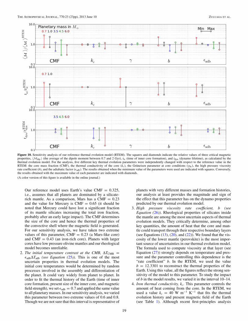
The Astrophysical Journal, 770:23 (23pp), 2013 June 10 Zuluaga et al.
Figure 10. Sensitivity analysis of our reference thermal evolution model (RTEM). The squares and diamonds indicate the relative values of three critical magneticproperties, 〈Mdip 〉 (the average of the dipole moment between 0.7 and 2 Gyr), tic (time of inner core formation), and tdyn (dynamo lifetime), as calculated by thethermal evolution model. For the analysis, five different key thermal evolution parameters were independently changed with respect to the reference value in theRTEM: the core mass fraction (CMF), the thermal conductivity of the core (kc), the Gruneisen parameter at core conditions (γ0c), the high pressure viscosityrate coefficient (b), and the adiabatic factor (εadb). The results obtained when the minimum value of the parameters were used are indicated with squares. Conversely,the results obtained with the maximum value of each parameter are indicated with diamonds.
(A color version of this figure is available in the online journal.)
Our reference model uses Earth’s value CMF = 0.325,i.e., assumes that all planets are dominated by a silicate-rich mantle. As a comparison, Mars has a CMF = 0.23and the value for Mercury is CMF = 0.65 (it should benoted that Mercury could have lost a significant fractionof its mantle silicates increasing the total iron fraction,probably after an early large impact). The CMF determinesthe size of the core and hence the thermal properties ofthe convective shell where the magnetic field is generated.For our sensitivity analysis, we have taken two extremevalues of this parameter, CMF = 0.23 (a Mars-like core)and CMF = 0.43 (an iron-rich core). Planets with largercores have low pressure olivine mantles and our rheologicalmodel becomes unreliable.
2. The initial temperature contrast at the CMB, ΔTCMB =εadbΔTadb (see Equation (25)). This is one of the mostuncertain properties in thermal evolution models. Theinitial core temperatures would be determined by randomprocesses involved in the assembly and differentiation ofthe planet. It could vary widely from planet to planet. Inorder to fit the thermal history of the Earth (time of innercore formation, present size of the inner core, and magneticfield strength), we set εadb = 0.7 and applied the same valueto all planetary masses. In our sensitivity analysis, we variedthis parameter between two extreme values of 0.6 and 0.8.Though we are not sure that this interval is representative of
planets with very different masses and formation histories,our analysis at least provides the magnitude and sign ofthe effect that this parameter has on the dynamo propertiespredicted by our thermal evolution model.
3. High pressure viscosity rate coefficient, b (seeEquation (26)). Rheological properties of silicates insidethe mantle are among the most uncertain aspects of thermalevolution models. They critically determine, among otherkey quantities, the amount of heat that the core and man-tle could transport through their respective boundary layers(see Equations (13), (20), and (22)). We found that the vis-cosity of the lower mantle (perovskite) is the most impor-tant source of uncertainties in our thermal evolution model.The formula used to compute viscosity at that layer (seeEquation (27)) strongly depends on temperature and pres-sure and the parameter controlling this dependence is the“rate coefficient” b. In the RTEM, we used the valueb = 12.3301 to reconstruct the thermal properties of theEarth. Using this value, all the figures reflect the strong sen-sitivity of the model to this parameter. To study the impactof b in the model results, we varied it in the interval 10–14.
4. Iron thermal conductivity, kc. This parameter controls theamount of heat coming from the core. In the RTEM, weused a value kc = 40 W m−1 K−1 that fits the thermalevolution history and present magnetic field of the Earth(see Table 1). Although recent first-principles analysis
19

The Astrophysical Journal, 770:23 (23pp), 2013 June 10 Zuluaga et al.
suggests that values as large as 150–250 W m−1 K−1
could be common at Earth’s core conditions (Pozzo et al.2012), we conform here to the standard values of thisparameter. Further investigations to explore values as largeas those found by Pozzo et al. (2012) should be attempted.For our sensitivity analysis, we varied kc between 35 and70 W m−1 K−1, two values which are inside the typicaluncertainty assumed for this property.
5. Gruneisen parameter for iron, γ0c. This is one of the mostcritical parameters of the equation of state, especially atcore conditions. It strongly affects the mechanical structure,temperature profile, and phase of iron in the metallic core(for a detailed discussion on the sensitivity of interiorstructure models to this parameter, see, e.g., VAL06). Inthe RTEM, we used the reference value γ0c = 1.36 that fitsthe thermal evolution history and present magnetic field ofthe Earth (see Table 1). Assuming different kinds of corealloys, a relatively large range of values of this parameterhave been used in literature (see VAL06 and referencestherein). The Gruneisen parameter values have been foundin the range of 1.36–2.338. Since our RTEM value is at thelower end of this range, for our sensitivity analysis we haverecalculated the model for a larger value of 2.06.
Other uncertain parameters, such as the critical Rayleighnumber at the CMB, Rac, which is also varied to study thesensitivity of thermal evolution models (E. Gaidos 2011, privatecommunication), were also studied. We did not find significantsensitivity of our model to the variation of those parameters.
In Figure 10 we depict the relative variation in the aforemen-tioned magnetosphere and dynamo properties when each of thepreviously described parameters were varied independently.
We found that planetary composition (CMF) and mantleviscosity are responsible for the largest uncertainties in thepredicted magnetic properties of the planet. Planets with smallmetallic cores have on average low magnetic dipole moments(squares in the first column of the upper panel). This is mainlydue to a geometrical effect. The total heat produced by the coreand hence the magnetic field strength at the core surface is ofthe same order as Fe-poor and Fe-rich planets. However, a smallcore also means a lower magnetic dipole moment, i.e.,M ∼ R3
c .Planets with lower iron contents also have small and hot coresand therefore the solid inner core formation and shutting downthe dynamo are slightly delayed (squares in the middle andlowest panel of Figure 10).
Viscosity dependence on pressure and temperature, as quan-tified by the parameter b, has the opposite effect on planetarymagnetic properties than CMF at least for EPs. A low viscosity,lower mantle will favor the extraction of heat from the metalliccore increasing the available convective energy for dynamo ac-tion. On the other hand, a viscous lower mantle will delay theformation of a solid inner core and extend the lifetime of thedynamo (middle and lowest panel in Figure 10).
The effect of the Gruneisen parameter at core conditions isnegligible, at least in respect to the magnetic field strength andlifetime (upper and lower panels) which are the most criticalproperties affecting planetary magnetic protection. Only thetime of the inner core formation is strongly affected by changesin this parameter. In planets smaller than Earth, inner coresolidification can be delayed up to three times the referencevalue. On the other hand, with a larger Gruneisen parameter, theinner cores of EPs could become solid very early in their thermalhistories, even almost from the beginning. This is a result of the
interplay between the resulting evolution of the thermal profileand the solidus.
The effect of the initial temperature contrast across the CMB,quantified by the parameter εadb, goes in the same directionas viscosity. The reasons for this behavior are, however, farmore complex. A larger initial temperature contrast acrossthe CMB also implies a larger initial temperature at the corecenter. Although a hotter core also produces a larger amountof available convective energy, the time required for iron toreach the solidification temperature is also larger. The dynamoof planets with Mp < 2 M⊕ and hot cores (large εadb) is weakerthan that of more massive planets during the critical first coupleof gigayears where the average is calculated. Planets with coldercores develop solid inner cores almost from the beginning andthe release of latent and gravitational energy feeds strongerdynamos.
The case of more massive planets, Mp > 2 M⊕, where thecondition for an inner core formation is never reached during thedynamo lifetime, is different. In this case, planets with hot cores(large lower mantle viscosities or high temperature contrastsalong the CMB) produce large amounts of available convectiveenergy. A larger convective power will produce a larger value ofthe local Rossby number. Thus, massive planets with hot coresalso have multipolar dynamos and hence lower dipole magneticmoments and a reduced magnetic protection.
Thermal conductivity affects the results of the thermal evo-lution model less. Besides the case of massive planets wheredifferences on the order of 10%–30% in the magnetic proper-ties are observed when kc varies between its extremes, the mag-netic properties calculated with our RTEM seem very robust incomparison with variations of these two properties. However, itshould be mentioned that this result applies only when a stan-dard value of kc is assumed. Further investigations to explorethe recent findings (Pozzo et al. 2012) concerning the possibil-ity that kc could be larger by factors as large as 2–3 should beattempted.
In summary, despite the existence of a natural sensitivityof our simplified thermal evolution model to uncertainties ontheir free parameters, the results presented in this paper seem tobe correct at least on the order of magnitude. Moreover, sincethe standoff distance and polar cap areas, which are the actualproxies to magnetic protection, goes as M1/3, a one order ofmagnitude estimation of M will give us an estimation of thelevel of magnetic protection by a factor of around two.
To clarify this point, let us consider the case of GL 581d. If weassume, for example, that its iron content is much less than thatof the Earth (as was assumed in the RTEM model), but the rest ofcritical thermal properties are essentially the same, the averagestandoff distance (polar cap area) at the critical first gigayear willbe off by only ∼30% with respect to the prediction depicted inFigure 9. More interesting is to note that the uncertainties due tothe unknown period of rotation (shaded area in Figure 9) seemto be much larger than those coming from the uncertainties inthe thermal evolution model.
7.3. Observational Support
Validating or improving thermal evolution models and dy-namo scaling laws for the case of SEs presently representsa huge observational challenge. The available sensitivity ofour best instruments on Earth and in space is rather insuf-ficient. New and/or improved instruments and observationaltechniques will be required to detect, catalog, and comparethe thermal and magnetic properties of low-mass planets in
20

The Astrophysical Journal, 770:23 (23pp), 2013 June 10 Zuluaga et al.
the future. However, the importance that the detection andcharacterization of the magnetic properties of potentially habit-able planets discovered in the future in order to assess their truehabitability clearly justifies the effort.
The first goal seems to be the direct or indirect detection ofSE magnetospheres. Four methods, some of which are alreadyused in our own solar system, could be devised to achieve thisgoal: (1) the detection of radio waves coming from synchrotronand cyclotron radiation produced by plasma trapped in the mag-netosphere, (2) the detection of a bow shock or a tail of ions pro-duced by the interaction of the planetary atmosphere and mag-netosphere with the stellar wind or the interplanetary plasma,(3) the detection of planetary auroras, and (4) spectroscopic ob-servations of a non-equilibrium atmospheric chemistry inducedby a high flux of CR (this is actually a negative detection of amagnetosphere).
The first (radio emission) and second methods (bow shockor tail) have already been studied in detail (Bastian et al. 2000;Farrell et al. 2004; Grießmeier et al. 2007b; Lazio et al. 2009;Vidotto et al. 2010, 2011). Its reliability, at least for the case ofplanets with intense magnetic fields or placed very close to theirhost star, has been already tested.
If synchrotron or cyclotron radiation coming from the magne-tosphere of TPs could be detected, the power and spectra of theradiation could be used to measure the magnetic field strength.However, even with the most sensitive instruments, e.g., the LowFrequency Array or the Long Wavelength Array, the expectedpower and spectra are several orders of magnitude below thethreshold of detection. Powers as large as 103–105 times theJupiter radio emission and frequencies in the range of tens ofMHz are required for the present detection of synchrotron ra-dio emission in planetary magnetospheres (see, e.g., Grießmeieret al. 2007b). The magnetic field intensities and expected fre-quencies produced in SEs magnetospheres are several orders ofmagnitude lower than these thresholds and are not likely to bedetected in the near future.
It has been shown recently that measurements of the asym-metry in the ingress and egress of transiting planets can be usedto detect the presence of a bow shock or a tail of plasma aroundthe planet. Vidotto et al. (2010, 2011) used this phenomenon toconstrain the magnetic properties of Wasp-12b. The formationof a detectable bow shock depends, among other factors, on therelative velocity between the planet and the shocked plasma.Close-in planets with strong enough magnetic fields (this is pre-cisely the case of Wasp-12b) can easily develop UV-opaque bowshocks and allow reliable detection. However, low-mass planetswith relatively weak magnetic fields, such as those predictedwith our models, hardly produce a detectable bow shock. It hasbeen estimated that magnetopause fields in the range of sev-eral gauss (among other important factors such as large enoughprojected magnetospheric size) should be required to have a de-tectable signal of a bow shock (A. A. Vidotto 2012, private com-munication). Our habitable SEs have magnetopause fields of theorder of a few microgauss (see Figure 7). The case of an ion tailcoming from a weakly magnetized planet has received less atten-tion and probably could offer better chances for a future indirectdetection of the magnetic environment of low-mass planets.
Finally, the detection of far-UV (FUV) or X-ray emissionfrom planetary auroras can also be used as a tool to directly andindirectly study planetary magnetospheres. Planetary auroraswith intensities as high as 102–103 times larger than that of theEarth are expected in close-in giant planets subject to the effectsof CMEs from its host star (Cohen et al. 2011). If we estimate
that a typical Earth aurora has an intensity of 1 kR (Neudegg et al.2001; being 1 R ∼ 10−11 photons m−2 s−1 sr−1) and assumingthat 10% of a close-in Jupiter-like planet is covered by aurorasproducing FUV photons around 130 nm, the total emitted powerfrom these planets will be ∼1013 W. If we assume that this is thepresent threshold for exoplanetary aurora detection, even understrong stellar wind conditions and distances typical of the HZ,the total FUV power produced by auroras in the polar cap ofEPs could be only 105 W, which is eight orders of magnitudeless than the present detection threshold. In addition, the FUVradiation should be detected against an intense UV backgroundlikely coming from a young and active low-mass star. If wecan find ways to overpass these difficulties, the observation ofthe FUV and X-ray emission and its variability from auroras inpotentially habitable SEs could be used as powerful probes ofthe magnetic environment around the planet.
8. SUMMARY AND CONCLUSIONS
We studied the influence that the thermal evolution of po-tentially habitable TPs has in the protection that an evolvingplanetary magnetosphere could provide against the atmosphericerosion caused by the stellar wind.
We developed a simple parameterized thermal evolutionmodel able to reproduce the global thermal history and magneticproperties of the past and present Earth. We applied this model topredict the thermal histories of planets with masses in the rangeof 0.5–6.0 M⊕ and with chemical compositions similar to Earth.Using these results and applying up-to-date dynamo scalinglaws, we predicted the magnetic properties of TPs in the HZ asa function of time, planetary mass, and rotation rate. A simplemodel of the evolution and interaction of the stellar wind withthe PMF, which has been adapted from previous works, allowedus to compute the global properties of the magnetosphere inorder to assess the level of magnetic protection that potentiallyhabitable EPs could actually have.
We applied our model to the case of potentially habitable TPsalready known (GL 581d, HD 40307g, and GJ 667Cc), to theEarth itself, and to the case of a hydrated Venus. In the case of theEarth, our model reproduces fairly well the early and presentthermal and magnetic properties of our planet. In the case ofthe hydrated Venus, the model predicts low values the standoffdistance and large polar cap areas in the first critical gigayear ofplanetary and thermal evolution, which are compatible with theidea that the planet lacked magnetic protection strong enoughto avoid a massive loss of water and volatiles that finally lead tothe shutdown of its dynamo ∼3 Gyr ago.
Compelling results were found in the case of the three extraso-lar system potentially habitable planets already discovered. As-suming an Earth-like composition and thermal evolution param-eters similar to those used in the case of the Earth (RTEM), ourmodel predicted that the dynamos of GL 581d and HD 40307ghave been already shut down. A younger GJ 667Cc seems tostill have an active dynamo.
A non-trivial dependence of the magnetic properties onplanetary age, planetary mass, and period of rotation has beenfound in general for terrestrial planets inside the HZ of theirhost stars. Thermal evolution is responsible for the non-trivialrelationship among all these properties. Contrary to that found inprevious works, tidally locked planets could develop relativelyintense magnetic fields and extended magnetospheres. However,they also have extended polar caps and likely multipolarmagnetic fields where field lines open to the interplanetary space
21

The Astrophysical Journal, 770:23 (23pp), 2013 June 10 Zuluaga et al.
and magnetotail regions, likely increasing the non-thermal masslosses.
Using recent results for the relationship between the exposi-tion to XUV radiation, the exobase radius, and mass-loss ratefrom massive SEs, we estimated the level of exposure and masslosses for the three potentially habitable SEs already discovered.With the information available little could be said about themagnetic protection of HD 40307g. Further theoretical investi-gations are required to evaluate this case. Our model predictsa magnetosphere large enough to protect GL 581d against theerosive action of the stellar wind during the first critical phasesof planetary evolution. However, since our model is still opti-mistic, further theoretical and observational analyses should beperformed to establish the magnetic protection of this planeton a more solid basis. Our upper limit to the standoff distanceand the most optimistic estimation of exobase radius and mass-loss rate from the atmosphere of GJ 667Cc point out the factthat this planet has already lost a large fraction of its inven-tory of volatiles. All the evidence compiled in this work makesGJ 667Cc a sort of “Venus analog.” Although further theoreticalanalyses are required, our best guess is that, despite the fact thatit is inside the radiative HZ of its host star, the planet is presentlyuninhabitable.
Last, but not least, we tested the robustness of our conclusionsby changing several of the most sensitive input parameters ofour thermal evolution model. We found that even under thepresent uncertainties the predicted properties of planetary mag-netospheres are rather robust. We calculated that introducinglarge variations in the composition of the planets and the rheo-logical and thermal properties of their interiors with respect tothe RTEM, the critical magnetic properties, such as the standoffradius and the area of the polar cap, change only by a factor oftwo. The results are also robust in comparison with uncertaintiesin the stellar wind properties that could be very important in thecase of close-in habitable planets around active and young dMstars.
The problem of evaluating the magnetic protection of poten-tially habitable planets is far from being settled. Other sources ofintrinsic magnetic fields, thermal evolution, and interior struc-ture of planets with “exotic” compositions, improved theoreti-cal models, and new experimental evidence of the behavior ofiron at high pressures and temperatures, improved and validatedmodels of the evolution and spatial structure of stellar windsand of course more and better observational data coming fromthe already discovered habitable SEs and future discovered po-tentially habitable exoplanets will allow us to assess the actualmagnetic protection of potentially habitable environments.
We appreciate the useful discussion and comments of Mer-cedes Lopez-Morales and other colleagues participating in theExploring Strange New Worlds 2011 Conference (Arizona, U.S.)and in the VI Taller de Ciencias Planetarias 2012 (Montevideo,Uruguay). Special thanks to Ignacio Ferrin who, with his cleverquestions and suggestions, originally motivated us to pursuesome of the goals of this work. We also thank Lisa Kalteneggerand Jeffrey Linsky for their insightful comments on preliminaryversions of this manuscript. We give special thanks to all our fel-low colleagues abroad who provided us with some key pieces ofliterature unobtainable in our country. We are grateful to AaronWest and Luke Webb for their careful revision of the English inthe manuscript. The remnant errors are all ours. An anonymousreferee is acknowledged for contributing significantly not onlyto the improvement of the manuscript but also to the quality of
the research conclusions. P.C. is supported by the Vicerrectoriade Docencia of the University of Antioquia. This work has beencompleted with the financial support of the CODI-UdeA underthe grant IN591CE and by the University of Medellin under thegrant number 530.
REFERENCES
Aubert, J., Labrosse, S., & Poitou, C. 2009, GeoJI, 179, 1414Baraffe, I., Chabrier, G., Allard, F., & Hauschildt, P. H. 1998, A&A, 337, 403Bastian, T. S., Dulk, G. A., & Leblanc, Y. 2000, ApJ, 545, 1058Batalha, N. M., Rowe, J. F., Bryson, S. T., et al. 2012, ApJS, 204, 24Bonfils, X., Delfosse, X., Udry, S., et al. 2011, arXiv:1111.5019BBorucki, W. J., Koch, D. G., Basri, G., et al. 2011, ApJ, 728, 117Boss, A. P. 2006, ApJL, 644, L79Catanzarite, J., & Shao, M. 2011, ApJ, 738, 151Chaufray, J. Y., Modolo, R., Leblanc, F., et al. 2007, JGRE, 112, 9009Christensen, U., Balogh, A., Breuer, D., & Glaßmeier, K. 2009, Planetary
Magnetism, Space Sciences Series of ISSI (New York: Springer)Christensen, U. R. 1985, JGR, 90, 2995Christensen, U. R. 2010, SSRv, 152, 565Cohen, O., Kashyap, V. L., Drake, J. J., Sokolov, I. V., & Gombosi, T. I.
2011, ApJ, 738, 166Denis, C., Rybicki, K. R., Schreider, A. A., Tomecka-Suchon, S., & Varga, P.
2011, AN, 332, 24Driscoll, P., & Olson, P. 2011, Icar, 213, 12Elkins-Tanton, L. T., & Seager, S. 2008, ApJ, 688, 628Farrell, W. M., Lazio, T. J. W., Desch, M. D., Bastian, T. S., & Zarka, P. 2004,
in IAU Symp. 213, Bioastronomy 2002: Life Among the Stars, ed. R. Norris& F. Stootman (San Francisco, CA: ASP), 73
Ferraz-Mello, S., Rodrıguez, A., & Hussmann, H. 2008, CeMDA, 101, 171Gaidos, E., Conrad, C. P., Manga, M., & Hernlund, J. 2010, ApJ, 718, 596Garces, A., Catalan, S., & Ribas, I. 2011, A&A, 531, A7Grenfell, J. L., Stracke, B., von Paris, P., et al. 2007, P&SS, 55, 661Grießmeier, J.-M., Khodachenko, M., Lammer, H., et al. 2010, in IAU Symp.
264, Solar and Stellar Variability: Impact on Earth and Planets, ed. A. G.Kosovichev, A. H. Andrei, & J.-P. Rozelot (Cambridge: Cambridge Univ.Press), 385
Grießmeier, J.-M., Preusse, S., Khodachenko, M., et al. 2007a, P&SS, 55, 618Grießmeier, J.-M., Stadelmann, A., Grenfell, J. L., Lammer, H., & Motschmann,
U. 2009, Icar, 199, 526Grießmeier, J.-M., Stadelmann, A., Motschmann, U., et al. 2005, AsBio, 5, 587Grießmeier, J.-M., Stadelmann, A., Penz, T., et al. 2004, A&A, 425, 753Grießmeier, J.-M., Zarka, P., & Spreeuw, H. 2007b, A&A, 475, 359Gubbins, D., Alfe, D., Masters, G., Price, G. D., & Gillan, M. 2004, GeoJI,
157, 1407Gubbins, D., Alfe, D., Masters, G., Price, G. D., & Gillan, M. J. 2003, GeoJI,
155, 609Guinan, E. F., Engle, S. G., & Dewarf, L. E. 2009, in AIP Conf. Ser. 1135, ed.
M. E. van Steenberg, G. Sonneborn, H. W. Moos, & W. P. Blair (Melville,NY: AIP), 244
Heller, R., Barnes, R., & Leconte, J. 2011, OLEB, 41, 539Henning, W. G., O’Connell, R. J., & Sasselov, D. D. 2009, ApJ, 707, 1000Joshi, M. M., Haberle, R. M., & Reynolds, R. T. 1997, Icar, 129, 450Judge, P. G., Solomon, S. C., & Ayres, T. R. 2003, ApJ, 593, 534Kaltenegger, L. 2010, ApJL, 712, L125Kaltenegger, L., Udry, S., & Pepe, F. 2011, arXiv:1108.3561Kasting, J. 2010, How to Find a Habitable Planet (Princeton, NJ: Princeton
Univ. Press)Kasting, J. F., Whitmire, D. P., & Reynolds, R. T. 1993, Icar, 101, 108Khodachenko, M. L., Ribas, I., Lammer, H., et al. 2007, AsBio, 7, 167Kipping, D. M., Bakos, G. A., Buchhave, L., Nesvorny, D., & Schmitt, A.
2012, ApJ, 750, 115Kite, E. S., Gaidos, E., & Manga, M. 2011, ApJ, 743, 41Kite, E. S., Manga, M., & Gaidos, E. 2009, ApJ, 700, 1732Kopparapu, R. K., Ramirez, R., Kasting, J. F., et al. 2013, ApJ, 765, 131Kulikov, Y. N., Lammer, H., Lichtenegger, H. I. M., et al. 2006, P&SS, 54, 1425Labrosse, S. 2003, PEPI, 140, 127Labrosse, S., Poirier, J.-P., & Le Mouel, J.-L. 2001, E&PSL, 190, 111Lammer, H., Bredehoft, J. H., Coustenis, A., et al. 2009, A&ARv, 17, 181Lammer, H., Lichtenegger, H. I. M., Khodachenko, M. L., Kulikov, Y. N., &
Griessmeier, J. 2012, in ASP Conf. Ser. 450, The Loss of Nitrogen-richAtmospheres from Earth-Like Exoplanets within M-star Habitable Zones,ed. J. P. Beaulieu, S. Dieters, & G. Tinetti (San Francisco, CA: ASP), 139
Lammer, H., Lichtenegger, H. I. M., Kulikov, Y. N., et al. 2007, AsBio, 7, 185Lammer, H., Ribas, I., Grießmeier, J.-M., et al. 2004, HvaOB, 28, 139
22

The Astrophysical Journal, 770:23 (23pp), 2013 June 10 Zuluaga et al.
Lammer, H., Selsis, F., Chassefiere, E., et al. 2010, AsBio, 10, 45Lammer, H., Selsis, F., Ribas, I., et al. 2003, ApJL, 598, L121Lazio, J., Bastian, T., Bryden, G., et al. 2009, Astronomy, Vol. 2010, Astro2010:
The Astronomy and Astrophysics Decadal Survey, Science White Papers,No. 177
Leconte, J., Chabrier, G., Baraffe, I., & Levrard, B. 2010, A&A, 516, A64Lopez-Morales, M., Gomez-Perez, N., & Ruedas, T. 2011, OLEB, 41, 533Manga, M., Weeraratne, D., & Morris, S. J. S. 2001, PhFl, 13, 802Mayor, M., Bonfils, X., Forveille, T., et al. 2009, A&A, 507, 487Mayor, M., & Udry, S. 2008, PhST, 130, 014010Mead, G. D. 1964, JGR, 69, 1181Miguel, Y., & Brunini, A. 2010, MNRAS, 406, 1935Neudegg, D. A., Cowley, S. W. H., McWilliams, K. A., et al. 2001, AnGeo,
19, 179Newkirk, G., Jr. 1980, in The Ancient Sun: Fossil Record in the Earth, Moon
and Meteorites, ed. R. O. Pepin, J. A. Eddy, & R. B. Merrill (New York:Pergamon), 293
Nimmo, F. 2009, Treatise on Geophysics, Vol. 8 (Amsterdam: Elsevier), 31Nimmo, F., & Stevenson, D. J. 2000, JGR, 105, 11969Olson, P., & Christensen, U. R. 2006, E&PSL, 250, 561Papuc, A. M., & Davies, G. F. 2008, Icar, 195, 447Parker, E. N. 1958, ApJ, 128, 664Peale, S. J. 1977, in IAU Colloq. 28: Planetary Satellites, ed. J. A. Burns (Tucson,
AZ: Univ. Arizona Press), 87Pepe, F., Lovis, C., Segransan, D., et al. 2011, A&A, 534, A58Pozzo, M., Davies, C., Gubbins, D., & Alfe, D. 2012, Natur, 485, 355Preusse, S., Kopp, A., Buchner, J., & Motschmann, U. 2005, A&A, 434, 1191Rauer, H., Gebauer, S., Paris, P. V., et al. 2011, A&A, 529, A8Ricard, Y. 2009, Treatise on Geophysics, Vol. 7 (Amsterdam: Elsevier), 6054Scalo, J., Kaltenegger, L., Segura, A. G., et al. 2007, AsBio, 7, 85Schubert, G., Cassen, P., & Young, R. E. 1979, Icar, 38, 192Schubert, G., Turcotte, D. L., & Olson, P. 2001, Mantle Convection in the Earth
and Planets (Cambridge: Cambridge Univ. Press)Schwenn, R. 1990, Large-Scale Structure of the Interplanetary Medium (Berlin:
Springer), 99Segura, A., Walkowicz, L. M., Meadows, V., Kasting, J., & Hawley, S. 2010,
AsBio, 10, 751
Selsis, F., Kasting, J. F., Levrard, B., et al. 2007, A&A, 476, 1373Siscoe, G., & Christopher, L. 1975, GeoRL, 2, 158Siscoe, G., & Crooker, N. 1976, JGG, 28, 1Siscoe, G. L., & Chen, C.-K. 1975, JGR, 80, 4675Stacey, F. D. 1992, Physics of the Earth (Brisbane: Brookfield Press)Stamenkovic, V., Breuer, D., & Spohn, T. 2011, Icar, 216, 572Stamenkovic, V., Noack, L., Breuer, D., & Spohn, T. 2012, ApJ,
748, 41Stevenson, D. J. 1983, RPPh, 46, 555Stevenson, D. J. 2003, E&PSL, 208, 1Stevenson, D. J. 2010, SSRv, 152, 651Tachinami, C., Senshu, H., & Ida, S. 2011, ApJ, 726, 70Tarduno, J. A., Cottrell, R. D., Watkeys, M. K., et al. 2010, Sci, 327, 1238Tian, F. 2009, ApJ, 703, 905Tian, F., Kasting, J. F., Liu, H.-L., & Roble, R. G. 2008, JGRE, 113, 5008Tuomi, M., Anglada-Escude, G., Gerlach, E., et al. 2012, A&A, 549, A48Udry, S., Bonfils, X., Delfosse, X., et al. 2007, A&A, 469, L43Underwood, D. R., Jones, B. W., & Sleep, P. N. 2003, IJAsB, 2, 289Valencia, D., O’Connell, R. J., & Sasselov, D. 2006, Icar, 181, 545Valencia, D., Sasselov, D. D., & O’Connell, R. J. 2007, ApJ, 665, 1413Varga, P., Denis, C., & Varga, T. 1998, JGeod, 25, 61Vidotto, A. A., Jardine, M., & Helling, C. 2010, ApJL, 722, L168Vidotto, A. A., Jardine, M., & Helling, C. 2011, MNRAS, 411, L46Voigt, G. 1995, Handbook of Atmospheric Electrodynamics, Vol. 2 (Boca Raton,
FL: CRC Press), 333Ward, P., & Brownlee, D. 2000, Rare Earth: Why Complex Life is Uncommon
in the Universe (New Yokr: Copernicus Books)Watson, A. J., Donahue, T. M., & Walker, J. C. G. 1981, Icar, 48, 150Weber, E. J., & Davis, L., Jr. 1967, ApJ, 148, 217Weinstein, S. A. 1992, E&PSL, 113, 23Wood, B. E., Muller, H.-R., Zank, G. P., & Linsky, J. L. 2002, ApJ,
574, 412Wood, B. E., Muller, H.-R., Zank, G. P., Linsky, J. L., & Redfield, S. 2005, ApJL,
628, L143Yamazaki, D., & Karato, S. 2001, AmMin, 86, 385Zendejas, J., Segura, A., & Raga, A. C. 2010, Icar, 210, 539Zuluaga, J. I., & Cuartas, P. A. 2012, Icar, 217, 88
23