the influence of operating cycle, cash flow volatility

SIJDEB, 4(1), 2020, 1-20 p-ISSN: 2581-2904, e-ISSN: 2581-2912 DOI: https://doi.org/10.29259/sijdeb.v4i1.1-20 Received: 11 January 2020; Accepted: 30 May 2020

SRIWIJAYA INTERNATIONAL JOURNAL OF DYNAMIC ECONOMICS AND BUSINESS

The Influence of Operating Cycle, Cash Flow Volatility, and Audit Fee on Earnings Persistence (The Indonesian

Cases)

Douglas 1, I Gusti Ketut Agung Ulupui2, and Hafifah Nasution3 1,2,3 Jakarta State University

[email protected] Abstract: Research is aiming at analyzing the influence of operating cycle, cash flow volatility, and audit fee on earnings persistence by studying manufacturing companies listed on Indonesia Stock Exchange (IDX). This research studied secondary data from documents in the forms of annual reports and financial reports of the companies taken from IDX website. After conducting a purposive sampling method, 12 companies were chosen to be the samples with 60 total observations. The data were analyzed by using descriptive statistics and panel data regression using Common Effect Model (CEM) processed by Eviews 10. Earnings persistence as the dependent variable was proxied by the regression coefficient from the regression model of previous year earnings towards the current earnings. The independent variable operating cycle was proxied by the means of accounts receivable turnovers and the means of the inventory turnovers. The cash flow volatility was proxied by the standard deviation of the cash flow operation divided by the total assets. The audit fee was proxied by the natural logarithm of the amount of audit fee. The panel data regression analysis showed that operating cycle has significant influence on earnings persistence. The results explain that companies with shorter operating cycle have high earnings persistence. The results also showed that cash flow volatility and audit fee have no influence on earnings persistence. A short operating cycle can make a company’s earnings persistence higher. The implication of this research is a shorter operating cycle can increase the earnings persistence of a company and can increase the interests of investors towards the company. Keywords: earnings persistence; operating cycle; cash flow volatility; audit fee;

manufacturing sector.

1Corresponding author

Douglas, Ulupui and Nasution/ SIJDEB, 4(1), 2020, 1-20

2

Introduction Stock Echange in Indonesia experienced an improvement in 2018 shown by a significant growth of Single Investor Identification (SID). Investors obtained SID to simplify the identification process and to serve as the basis for various future improvements in stock exchange. A press release from Kustodian Sentral Efek Indonesia (KSEI) issued in its website on 27 December 2018 stated that the number of SID had increased by 44% to 1.613.165 SID since the end of December 2017 until 26 December 2018. Investors must be familiar with the companies they want to invest in before making investment decisions. This is crucial as they do not want to suffer losses from their investment. This is why investors should get to know the prospective companies they want to invest in by looking at their field of business, the companies’ management, and their performance. A company’s performance can be seen from its financial statements showing the balance sheet, income statement, and statement of cash flow which are useful for the financial statements users when making economic decisions (PSAK No. 1, 2018). The financial statement shows the management’s accountability of the company’s resources they use. A big profit made by a company indicates a good performance. A company can obtain a profit or suffer a decrease in profit in an instant. For example, PT Semen Indonesia TbK (SMGR) booked a net profit of Rp412 billion during Q1 2018. This amount is a significant decrease by 44% from that of Q1 2017 which had reached Rp747 billion. PT Tirta Mahakam Resources Tbk (TIRT) had a net profit of Rp1,16 billion in Q1 2018 which is a significant drop by 76,93% of the net profit in Q1 2017 which had reached Rp5,06 billion. An even higher percentage of decrease was suffered by PT KMI Wire and Cable Tbk (KBLI). Having booked a profit of Rp222,5 billion in the first semester of 2017, KLBI suffered a dramatic fall by 82,78% in the first semester of 2018 when it booked a profit of Rp38,3 billion. The three companies are manufacturing companies. In Indonesia Economic Outlook 2019 discussion (8/1/2019), the Minister of Industry, Airlangga Hartanto, said that the manufacturing sector contributes to GDP by 20%, to tax by around 30%, and to export by 74% (www.ekbis.sindonews.com). The figures show that manufacturing sector is important for the economy of Indonesia. Earnings persistence is one of the indicators to assess the quality of a company’s profit. Fanani (2010) asserted that earnings persistence refers to expected accounting profit or expected future earnings which can be reflected from the current earnings. Earning persistence is related to the overall performance of a company as indicated by the company’s profit. High earnings persistence is indicated by profits generated continuously in a relatively long period. In addition, earnings persistence is also related to the performance of stock prices in stock markets which produces yields. This strengthens the relation between the company’s profits and the yields obtained by investors in high stock return. When a company can sustain current earnings which can serve as a good indicator of future earnings, the company has earnings persistence (Annisa & Kurniasih, 2017).


3

Operating cycle of a company is one of the factors which can be used to measure earnings persistence of the company. Operating cycle is the average period of time spent by a company to obtain inventories and sell the inventories to its customers to get cash income (Fanani, 2010). In other words, operating cycle is a sequence of activities done by a company starting from the procurement of supplies to be sold to the customers to the collection of payment from the customers to the company as revenues. The company’s earnings can be predicted from the operating cycle as it includes the selling factor which can be used to calculate earnings. Fauzia, rahmadani, & Nurhayati (2016) confirmed that the operating cycle influences the earnings persistence. A shorter period of operating cycle can ensure the company obtains payment faster and gets some revenues. The payment obtained from the operating cycle is the current earnings which can be an indicator for the future earnings. This means the shorter the life cycle period is, the higher the earnings persistence of a company is. Fanani (2010) has a different opinion on the matter by concluding that the operating cycle does not influence the earnings persistence. This is because a longer operating cycle does not trigger significant uncertainty which affects accruals, and it barely helps in predicting future cash flows. In a nutshell, a longer operating cycle does not make the earnings persistence of a company lower. Cash flows of a company is one of the information needed by investors to assess the capability of the company to generate cash on hand and cash equivalent; and the company’s necessities to use them. To measure the earnings persistence of a company, an information of a relatively stable cash flow, which has lower volatility, is needed. When the cash flows of a company fluctuate dramatically, the high volatility makes it difficult to predict the future cash flows, and it also indicates uncertainty in operating cycle because the current earnings cannot be used to predict the future earnings (Fanani, 2010). Rahmadani (2016) concluded that cash flow volatility affects earnings persistence. Lower cash flow fluctuation means lower volatility, and this can also indicates higher earnings persistence because the current earnings information can be used to predict future earnings. On the other hands, Kasiono & Fachrurrozie (2016) are of the opinion that there is no relation between volatility level and earnings persistence because cash flow fluctuation cannokasiot be used to predict future earnings and earnings persistence. Another factor which can affect earnings persistence is audit fee. Audit fee is the amount of fees charged by auditors for conducting audit services on a company by considering engagement risk, given task complexities, the necessary expertise to perform the task, the cost structures of the public accounting firm (KAP) in question, and other professional considerations (Agoes, 2012, p.18). Nuraeni, Mulyati, & Putri (2018) confirmed that audit fee affects earnings persistence. The higher the audit fee is paid, the higher the earnings persistence increases. This is because a substantial amount of audit fee can support the audit firm to be more independent, and the fee can be used to prepare a more extensive and meticulous research and auditing procedures which result in higher quality of audit results. By hiring an external independent auditor, the management is compelled to boost the company’s performance, two of which is to report earnings quality or earnings persistence and to reduce earnings management practices. Whether or not operating cycle and cash flow volatility variables affect earnings persistence are still debatable. This is why the present research steps in to confirm the results of the previous research by adding audit fee variable, which still attracts less attention in research


4

on earnings persistence. The present research, thus, wants to study “the influence of operating cycle, cash flow volatility, and audit fee on earnings persistence.” The research problems of the present study is as follows: Does the operating cycle, cash flow volatility, audit fee affect earnings persistence? Research Objectives of this study to provide empirical evidence on the influence of operating cycle, cash flow volatility, audit fee on earnings persistence. Literature Review Signal ing Theory Signaling Theory was first introduced by Spence (1973) when he proposed that senders (information source) attempt to send a ‘signal’, i.e. pieces of relevant information, which are useful for the receivers who will adjust their behavior according to their interpretation of the signal. Management of a company send ‘signals’ to stock markets by publishing information about the company to public. This signaling from the management reduces information asymmetry for the investors who may respond differently depending on their interpretation of the signal which can serve as the basis of consideration for the investors to make investment decisions. Earning persistence is one of the signals needed by investors to make decisions. Investors can conclude that a company with earnings persistence is able to maintain the sustainability of its business, and, in turn, earnings persistence can attract the investors to invest capital in the company. A company with highly fluctuated and uncontrollable earnings attracts less investors because they will conclude the company is not able to maintain its sustainability. Thus, earnings persistence is a signal or information which needs to be reported to the the financial statements users or market participants to make decisions. Earnings Pers is t ence Earnings persistence refers to expected accounting profit or expected future earnings which can be reflected from the current earnings (Yao et.al, 2018).Earnings persistence is a type of earnings which is able to serve as an indicator of future earnings generated repetitively by a company for a long period (sustainable). Earning persistence is related to the overall performance of a company as indicated by the company’s profits. High earnings persistence is indicated by profits generated sustainably in a relatively long period. In addition, earnings persistence is also related to the performance of stock prices in stock markets which produces yields. This strengthens the relation between the company’s profits and the yields obtained by investors in high stock return. When a company can sustain current earnings which can serve as a good indicator of future earnings, the company has earnings persistence (Annisa & Kurniasih, 2017). Earnings persistence can be considered as an indicator that a company has been successful in running its business within certain periods of time. In other words, when a company’s earnings are persistence, the company is running its business sustainably well, whereas when the earnings of a company fluctuate significantly and uncontrollably, the company is considered as unable to maintain the sustainability of the company’s business.


5

The Inf luence o f Operat ing Cyc le on Earnings Pers is t ence Operating cycle is a business cycle starting from the initial outlay of cash to the time when cash is received as revenues (Prihadi, 2012, p.32). Operating cycle is the total days needed to convert the inventory and accounts receivable into cash. Operating cycle depends on the company policy on: a. Inventory: how long it stays in storage. A longer time extends the cycle. b. Sales: cash or credit. If a company sells in cash, it incurs no business debt. However, if

the company sells on credit, it incurs accounts receivable. A long collection period of debt will extend the operating cyle.

c. Purchase: cash or credit. Credit purchase reduce the length of operating cycle. Operating cycle is the average period of time spent by a company to obtain supplies and sell the supplies to its customers to get cash income (Fanani, 2010). In other words, operating cycle is a sequence of activities done by a company starting from the procurement of inventory to be sold to the customers to the collection of payment from the customers to the company as revenues. The company’s earnings can be predicted from the operating cycle as it includes the selling factor which can be used to calculate earnings. Fauzia, Sukarmanto, & Nurhayati (2016) did a study on mining companies listed on Indonesia Stock Exchange (IDX) within 2012–2014 and confirmed that the operating cycle influences the earnings persistence. A shorter period of operating cycle can ensure the company obtains payment faster and gets some revenues. The payment obtained from the operating cycle is the current earnings which can be an indicator for the future earnings. This means the shorter the life cycle period is, the higher the earnings persistence of a company is. Similar results are also found in Lee, Panjaitan, & Hasibuan (2018) and Susilo & Anggraeni (2016). On the other hand, Fanani (2010) who did a study on manucturing companies listed on IDX within 2001–2006 concluded that the operating cycle does not influence the earnings persistence. This is because a longer operating cycle does not trigger significant uncertainty which affects accruals, and it barely helps in predicting future cash flows. In a nutshell, a longer operating cycle in a budget year does not make the earnings persistence of a company lower. Proposed hypothesis: Operating cycle affects earnings persistence. The Inf luence o f Cash Flow Volat i l i ty on Earnings Pers is tenc e Cash flow of a company is the company’s means to generate and spend their cash fund. Cash flow provides historical information on the changes in cash on hand and cash equivalent. The Great Dictionary of Indonesian Language (KBBI) defines cash flow as company’s cash on hand expenditure and income measured daily, weekly, or other time period. There are two types of cash flow in a company: a. Cash inflow, generated from external sources (e.g. from the owner, capital investment,

equity sales, and bank loans) and internal sources (utilization of fixed assets, inventory, and others).


6

b. Cash outflow, external use (liability payment) and internal use (cash used to obtain fixed assets, inventory, investments, and business expansion).

Dechow & Dichev (as cited in Fanani, 2010) defines cash flow volatility as the degree of cash flow distribution or the company’s cash flow distribution index. Investors need cash flow information to assess the capability of a business entity to generate cash and cash equivalent and to utilize them. To measure the earnings persistence of a company, an information of a relatively stable cash flow, which has lower volatility, is needed. When the cash flows of a company fluctuate dramatically, the high volatility makes it difficult to predict the future cash flows, and it also indicates uncertainty in operating cycle because the current earnings cannot be used to predict the future earnings (Fanani, 2010) Rahmadani (2016) who did a research on companies from various industries listed on IDX within 2010–2014 concluded that cash flow volatility affects earnings persistence. Lower cash flow fluctuation means lower volatility, and this can also indicate higher earnings persistence because the current earnings information can be used to predict future earnings. Similar results are also reported by Nuzula (2017), Indra (2014), and Hayati (2014). Kasiono & Fachrurrozie (2016) who did a research on manufacturing companies listed on IDX within 2011–2013 are of the opinion that there is no relation between volatility level and earnings persistence because cash flow fluctuation cannot be used to predict future earnings and earnings persistence. Similar results are found in Sutisna & Ekawati (2016). Proposed hypothesis: cash flow volatility affects earnings persistence. The Inf luence o f Audit Fee on Earnings Pers is tence Audit fee is the amount of fees charged by auditors for conducting audit services on a company by considering engagement risk, given task complexities, the necessary expertise to perform the task, the cost structures of the public accounting firm (KAP) in question, and other professional considerations (Agoes, 2012, p.18). Audit fee is a cost which must be covered by a company to get external auditor services. A substantial amount of audit fee can support the public accounting firm to be more independent, and the fee can be used to prepare a more extensive and meticulous research and auditing procedures which result in higher quality of audit results (Nuraeni, Mulyati, & Putri, 2018). In 2016, Indonesian Public Accounting Institute (IAPI) issued Management Regulation No.2 on The Pricing of Financial Report Audit Service used as a guideline for public accounting professions, public accounting firms, and IAPI members to set the audit fees for their professional services as public accountants. Nuraeni, Mulyati, & Putri (2018) who did a research on property and real estate companies listed on IDX within 2013–2015 confirmed that audit fee affects earnings persistence. The higher the audit fee is paid, the higher the earnings persistence increases. This is because a substantial amount of audit fee can support the audit firm to be more independent, and the fee can be used to prepare a more extensive and meticulous research and auditing procedures which result in higher quality of audit results. This research supports the results of a research done by El-Gammal (2012) which concluded that multinational companies and banks in Lebanon prefers to pay higher audit fee because they want to hire auditors who can produce high quality financial reports and


7

who can increase the credibility of their annual financial reports which can help them compete globally. By hiring external independent auditors, the management is compelled to boost the company’s performance, two of which is to report earnings quality or earnings persistence and to reduce earnings management practices. The fluctuation of company’s earnings with significant changes has resulted in the doubts about its earnings persistence. As a matter of fact, earnings persistence is one of the important elements need to be considered by investors. A significant drop of earnings can be responded negatively by investors based on Signaling Theory. Proposed hypothesis: Audit fee affects earnings persistence. Methods Research Objec ts and Scope The research objects are manufacturing companies listed on Indonesia Stock Exchange (IDX) 2013–2017. The scope of this research involves earnings persistence variable which is limited based on the regression coefficient values of their after-tax annual earnings, operating cycle variable which is limited based on the total of accounts receivable turnovers which are added to the inventory turnovers, cash flow volatility variable which is limited based on the standard deviation of operational cash flow divided by the total assets, and audit fee variable which is limited based on the cost of audit paid by the companies to the public accounting firms as stated in their annual reports.

Research Method

Populat ion and Sampling The research population is a group of manufacturing companies listed on IDX within 2013–2017. The samples of data were taken by purposive sampling techniques. A set of criteria were formulated to be in line with the research objectives. The criteria of the companies are as follows. 1. Manufacturing companies listed on IDX within the period of 2013–2017. 2. The companies have consistently published their annual reports after being audited by

December 31st every year. 3. The companies gained earnings during the period of 2013–2017. 4. The companies used Indonesian Rupiah (IDR) as the presentation currency in their

annual reports. 5. The companies have complete data related to the three variables used in this research:

after-tax annual earnings, accounts receivable turnovers and inventory turnovers, comparison of the operational cash flow with the total assets and audit fee in their annual reports.

Operat ional Variables This research analyzed the influence of the independent variables, i.e. operating cycle, cash flow volatility, and audit fee, on the dependent variable, i.e. earnings persistence. The next section elaborates the operational variables.

1. Dependent Variables


8

Dependent variables are those which are influenced or which become affected by the independent variables. In this research, earnings persistence is the dependent variable. Conceptual Definition: Earnings persistence is the expected accounting profit or expected future earnings which can be reflected from the current earnings (Fanani, 2010). Operational Definition: Earnings persistence variable is measured by calculating the after-tax earnings regression by using an equation from Nuraeni, Mulyati, & Putri (2018):

Notes: Eit = Company’s earnings i year t �0 = Constant variable �1 = Regression coefficient Eit-1 = Company’s earnings i year t-1 �it = Error 2. Independent Variables The three independent variables in this research are operating cycle, cash flow volatility, and audit fee. The three variables are defined briefly in the following conceptual definition and operational definition.

a. Operating Cycle

Conceptual Definition: Operating cycle is a business cycle starting from the initial outlay of cash to the time when cash is received as revenues (Prihadi, 2012, p.32). Operating cycle is the total days needed to convert the inventory and accounts receivable into cash.

Operational Definition: The operating cycle variable is measured by adding the average of accounts receivabe turnovers to the average of inventory turnovers. This formula is also used by Fanani (2010), Susilo & Anggraeni (2016), and Lee, Panjaitan, & Hasibuan (2018).

Notes: 𝑂𝐶 = Operating Cycle (ARt+ARt-1) = Average of Account Receivables of Company i Year t Sales t = Sales (Invent+Invent-1) = Average of Inventory of Company i Year t COGS t = Cost of Goods Sold b. Cash Flow Volatility

Eit= β0+β1Eit-1+εit

𝑂𝐶 =(ARt+ARt-1)/2

Sales t/360+(Invent+Invent-1)/2

COGS t/360


9

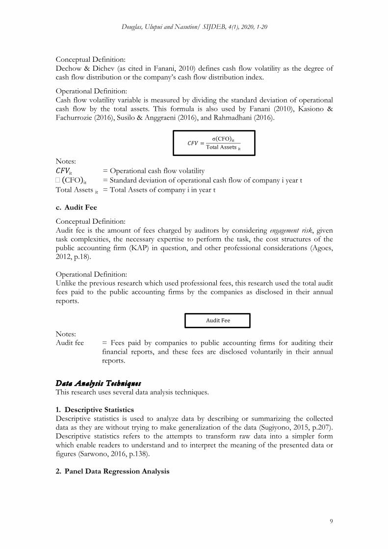
Conceptual Definition: Dechow & Dichev (as cited in Fanani, 2010) defines cash flow volatility as the degree of cash flow distribution or the company’s cash flow distribution index.

Operational Definition: Cash flow volatility variable is measured by dividing the standard deviation of operational cash flow by the total assets. This formula is also used by Fanani (2010), Kasiono & Fachurrozie (2016), Susilo & Anggraeni (2016), and Rahmadhani (2016).

Notes: 𝐶𝐹𝑉it = Operational cash flow volatility � CFO it = Standard deviation of operational cash flow of company i year t Total Assets it = Total Assets of company i in year t c. Audit Fee

Conceptual Definition: Audit fee is the amount of fees charged by auditors by considering engagement risk, given task complexities, the necessary expertise to perform the task, the cost structures of the public accounting firm (KAP) in question, and other professional considerations (Agoes, 2012, p.18).

Operational Definition: Unlike the previous research which used professional fees, this research used the total audit fees paid to the public accounting firms by the companies as disclosed in their annual reports.

Notes: Audit fee = Fees paid by companies to public accounting firms for auditing their

financial reports, and these fees are disclosed voluntarily in their annual reports.

Data Analys is Techniques This research uses several data analysis techniques. 1. Descriptive Statistics Descriptive statistics is used to analyze data by describing or summarizing the collected data as they are without trying to make generalization of the data (Sugiyono, 2015, p.207). Descriptive statistics refers to the attempts to transform raw data into a simpler form which enable readers to understand and to interpret the meaning of the presented data or figures (Sarwono, 2016, p.138).

2. Panel Data Regression Analysis

𝐶𝐹𝑉 =σ(CFO)it

Total Assets it

Audit Fee


10

This research has cross-sectional data and time series data; thus, the data are known as pooled data or panel data (Ghozali & Ratmono, 2017, p.195) Cross sectional data are the data from one or more objects gathered within a particular time, whereas time series data are those which are observed and taken from different time periods. There are two types of panel data regression: balanced panel data and unbalanced panel data. The panel data which are observed at the same period are balanced panel data. When the panel data are not observed at the same period or when some panel data are missing, the panel data are unbalanced. This research uses balanced panel data by observing the data within the same period. Any data which do not comply with purposive sampling criteria are discarded.

a. Regresion Equation Model The regression equation for panel data used in this research is as follows.

𝑬𝑷𝒊𝒕 = 𝜶𝟎𝒊𝒕 + 𝜷𝟏𝑶𝑪𝒊𝒕 + 𝜷𝟐𝑪𝑭𝑽𝒊𝒕 + 𝜷𝟑𝑭𝑬𝑬𝒊𝒕 + 𝒆𝒊𝒕

Notes: 𝛼! = Constant 𝛽!, 𝛽!, 𝛽! = Regression Coefficient EP = Earnings Persistence OC = Operating Cycle CFV = Cash Flow Volatility FEE = Audit Fee 𝑒 = Regression Error it = Object number –i and time –t

b. Classical Assumption Test

The classical assumption test includes normality test, multicollinearity test, autocorrelation test, and heteroscedasticity test. Hypothes i s Tes t ing a. T-Statistic Test A t-test is used to compare the means of two population of interval scale data (Sarwono, 2006, p.154). A t-test basically shows the influence degree of an independent variable to explain the variance of a dependent variable. The null hypothesis is a joint hypothesis that �1, �2..... �k are simultaneously equal to zero.

H0: �1 = �2 = ............= �k = 0

This joint hypothesis testing is also referred to as a test of the overall significance of the regression line which is aimed at testing whether Y has linear relation with both A1 and X2. A joint hypothesis can be tested by using Anova. If tcal > ttab t�(n-k), H0 is rejected, and X1 affects Y, Alpha (�) is the significance level and (n-k) is the degree of freedom taken from total n observation is substracted by the total of independent variables in the model (Ghozali & Ratmono, 2017, p.58).


11

If the significance level is higher than 0,05, the independent variables has no partial influence on the dependent variables. However, if the significance level is lower than 0,05, the independent variables has partial influence on the dependent variables.

b. F-Statistic Test F-test basically shows whether all independent variables put in a model has a simultaneous influence on the dependent variables. The F-test uses the following hypotheses: H0: Independent variables have simultaneous influence Ha: Independent variables have no simultaneous influence

If the test result is <0,05, H0 is accepted, and independent variables have simultaneous influence. However, if the result is >0,05, H0 is rejected and Ha is accepted, i.e. independent variables have no simultaneous influence.

c. Coefficient of Determination The coefficient of determination (R2) basically shows the capability of a model to interpret the variance in the dependent variables. The R2 value is between zero and one. The shortcoming of R2 is its bias towards the number of independent variables put in the model. This is why many experts suggest the use of adjusted R2 to assess the best regression model. Unlike R2, adjusted R2 can go up or down if an independent variable is added to the model (Ghozali & Ratmono, 2017, p.56). Mathematically, if R2 = 1, then adjusted R2 = 1, whereas if R2 = 0, then the adjusted R2= (1-k)/(n-k). If k>1, then the adjusted R2 will have negative value (Ghozali & Ratmono, 2017, p.56). A lower R2 value means that the capability of the independent variables to predict the dependent variables is limited. This also means that the variables of this research do not influence earnings persistence. If R2 value is almost one, it means that the independent variables provide almost all information needed to predict the dependent variables. This means the variables of this research influence earnings persistence.

Result and Discussion Descr ipt ion o f Data Description of data is divided into two: the results of sampling selection and the results of descriptive statistics: 1. Results of Sampling Selection

Table 1. Sampling Selection No. Description Total

1 Manufacturing companies listed on IDX within the period of 2013–2017. 159

2 The companies which had not consistently published their annual reports after being audited by December 31st every year of observation. (25)

3 The companies which had not used Indonesian Rupiah (IDR) as the presentation currency in their annual reports. (29)

4 The companies which had not gained earnings during the observation period. (44)

5 The companies which had not disclosed the amount of audit fees in their annual reports. (49)


12

Source: Data processed by the researchers (2019).

2. Analysis of Descriptive Statistics Table 2. Descriptive Statistics

EP OC CFV FEE Maximum 2,0399 307,339 0,17661 22,6293 Minimum -0,760 68,994 0,01788 19,0084

Mean 0,5368 146,920 0,05901 20,5234 Std. Dev. 0,6279 56,5642 0,03400 1,15138

N 60 60 60 60 Source: Data processed by the researchers (2019) Hypothes is Test ing The hypothesis testing consists of three parts: panel data regression test, classical assumption test, and the panel data regression test results. 1. Panel Data Regression Tests a. Chow Test Chow test is used to decide which model, between the common effect model or the fixed effect model, can be used to process the data more properly. The hypotheses in this Chow test:

H0 : Common Effect Model Ha : Fixed Effect Model

Based on the Chow test, the probability value of cross-section F is 0,4927 or higher than 0,05. This means H0 is accepted, and the common effect model is used.

b. Lagrange Multiplier Test Lagrange Multipler test is used to to decide which model, between the common effect model or the random effect model, can be used to process the data more properly. The proposed hypothese are:

H0: Common Effect Model Ha: Random Effect Model

Based on the Lagrange Multipler test, the probability values is 0,8312, or > 0,05. This means H0 is accepted, and the common effect model is used.

2. Classical Asumption Test a. Normality Test Normality test is aimed at testing whether the error variables or residuals have normally distributed in the regression model (Ghozali & Ratmono, 2017, p.145). The normality level of the distributed data becomes the initial reference to decide whether the research can be conducted or not.

Table 3. Normality Test

Total sample 12 Total observation in 5 years (2013-2017) 60


13

Source: Output Eviews 10 results (2019)

Based on the normality test, the Jarque-Bera probability value is 0,767027 or higher than 0,05. This means that the data in this research have normal distribution. b. Multicollinearity Test Multicollinearity test is aiming at assessing whether in the regression there is a high correlation among the independent variables (Ghozali & Ratmono, 2017, p.71).

Table 4. Multicollinearity Test

OC CFV FEEOC 1.000000 0.355207 -0.173619CFV 0.355207 1.000000 -0.514366FEE -0.173619 -0.514366 1.000000


Based on the multicollinearity test, there are no correlations among variables which exceed 0,8. Thus, it can be concluded that the independent variables in this research show no multicollinearity. c. Autocorellation Test Autocorrelation test is aimed at testing whether in the linear regression model there is a correlation between residuals in t-period and residuals in t-1 (previous year).

Table 5. Autocorrelation Test LM/BG Test


Based on the autocorrelation test, the probability Obs*R-squared is 0,0541 or higher than 0,05. Thus, it can be concluded that there is no correlation in the regression model. d. Heteroscedasticity Test Heteroscedasticity test is used to determine whether in the regression model there are variance inequalities from residuals of one observation to another.

Table 6. Heteroscedasticity Test


14

Variable Coefficient Std.Error t-Statistic Prob.

C 1.4172851 1.013702 1.393754 0.1689OC -0.000745 0.000872 -0.854937 0.3962CFV -1.318566 1.664906 -0.791976 0.4317FEE -0.039338 0.046674 -0.842841 0.4029


Based on the heteroscedasticity test by using glejser test, it is found that each independent variable has probability value higher than 0,05. Thus, it can be concluded that the data in this research is free from heteroscedasticity test.

3. Panel Data Regression Test Results After the data are tested by data panel regression model test and classical assumption test, the results of panel data regression test are presented here.

Table 7. Panel Data Regression Tests with Common Effec t Model

Dependent Variable: PL Method: Panel Least Squares Date: 06/13/19 Time: 18:42 Sample:2013 2017 Periods included: 5 Cross-sections included: 12 Total Panel (balanced) observations: 60

Variable Coefficient Std. Error t-Statistic Prob. C 0.262288 1.613267 0.162582 0.8714

OC -0.003503 0.001387 -2.525674 0.0144 CFV -4.054089 2.649633 -1.530057 0.1316 FEE 0.050115 0.074279 0.674689 0.5026

R-Squared 0.236243 Mean dependent var 0.536849 Adjusted R-Squared 0.195327 S.D dependent var 0.627983 S.E. of regression 0.563323 Akaike info criterion 1.754415 Sum squared resid 17.77066 Schwarz criterion 1.894038 Log likelihood -48.63244 Hannan-Quinn criter 1.809029 F-Statistic 5.773905 Durbin-Watson stat 1.515788 Prob(F-statistic) 0.001636


Based on the panel data regression test results shown in the table, the panel data regression equation is as follows.

EP = 0,2622 – 0,0035OC – 4,0540CFV + 0,0501FEE

Notes: EP = Earnings Persistence OC = Operating Cycle CFV = Cash Flow Volatility FEE = Natural Logarithm of Audit Fee a. Coefficient of Determination


15

Based on the panel data regression tests, the coefficient of determination value calculated by adjusted R2 is 0,1953 or 19,53%. This means the independent variables in the regression model can predict the dependent variables of earnings persistence by 19,53%, and the remaining 80,47% is explained by factors which are not included in the model.

b. F-Statistic Test F-test basically shows whether all independent variables put in a model has a simultaneous influence on the dependent variables. Based on the F-statistics tests, Fcal > Ftab isc5,7739 > 2,77, and the probability value is 0,0016 or lower than 0,05. Thus, it can be concluded that the three independent variables, i.e. operating cycle, cash flow volatility, and audit fee, simultaneously have significant influences on earnings persistence.

c. T-Statistic Test A t-test is done to identify the relation of an independent variable individually when predicting the variance of dependent variables. With df value at 57, which is obtained by subtracting the total samples (n) 60 with the independent variable (k) 3, the ttab is 2,00247. The t-test result is shown in Table IV.7.

From t-test table, the results of hypothesis testings can be obtained partially with regard of the influence of operating cycle, cash flow volatility, and audit fee on earnings persistence. 1) Hypotheses Testing 1 From the t-test, operating cycle has tcal of -2,5256 with probability value of 0,0144. This shows that tcal > ttab (-2,5256 > 2,00247), and p value is 0,0144 < 0,05. Thus, hypothesis 1 is accepted, and this means operating cycle variable has significant influence on earnings persistence.

2) Hypothesis Testing 2 From the t-test, cash flow volatility has tcal of -1,5300 with probability value of 0,1316. This shows that tcal < ttab (-1,5300 < 2,00247), and p value is 0,1316 > 0,05. Thus, hypothesis 2 is accepted, and this means that cash flow volatility variable has no influence on earnings persistence.

3) Hypothesis Testing 3 From the t-test, audit fee has tcal of r 0,6746 with probability value of 0,5026. This shows that tcal < ttab (0,5026 < 2,00247), and p value is 0,5026 > 0,05. Thus, hypothesis 3 is rejected. This means audit fee variable has no influence on earnings persistence. Discuss ion From the data testing and analyses, the next section briefly discusses the test results of the relations between each independent variable and the dependent variable.

1. Operating Cycle on Earning Persistence Based on t-test, this present research confirms that operating cycle has significant influence on earnings persistence. Based on signaling theory, investors look at the operating cycle of a company as a source of information on the duration of time used by the company to generate cash from the company’s main operations. The faster the operating cycle of a company is, the faster the company generates cash from its main operations, and this also


16

means that the company’s earnings can be predicted. If the operating cycle is slow, it gives signal that the company will also be slow in generating cash from its main companies, and this means the company’s earnings cannot be be predicted. Fauzia, Sukarmanto, & Nurhayati (2016) is of the opinin that a faster operating cycle, i.e. from the time cash is spent to buy inventories to the time when the inventories are sold, means a faster time. The income accepted within the operating cycle is the current earnings which can reflect future earnings (for the next period). A shorter time used to generate cash means a higher earnings persistence. Similar results were reported by Lee, Panjaitan, & Hasibuan (2018) and Susilo & Anggraeni (2016) who proved that operating cycle has a significant influence on earnings persistence. In other words, operating cycle is directly related to earnings persistence which can predict the future cash flows.

2. Cash Flow Volatility on Earnings Persistence Based on t-test, this present research also confirms that cash flow volatility has no influence on earnings persistence. Based on Signaling Theory, cash flow volatility can provide investors with information about a company’s cash flow fluctuation in certain periods. However, the facts showed that fluctuation in a company’s cash flow has no influence on the company’s earnings persistence. This result is in line with that of Kasiono & Fachrurrozie (2016) which also confirmed that cash flow volatility has no influence of earnings persistence. This is mainly because of an implicit assumption which becomes the basis of cash flow quality. The assumption is that there are cross-sectional variations in the capabilities of managers to manipulate the cash flow volatility report; thus, investors do not really take cash flow volatility into considerations when determining the earnings persistence level (Kasiono & Fachrurrozie, 2016).

3. Audit Fee on Earnings Persistence Based on t-test, the present research confirms that audit fee has no influence on earnings persistence. Based on Signaling Theory, audit fee is an information provided for the investors about the amount of fee paid by a company to guarantee the quality of its financial reports. The amount of audit fee can be set by looking at several aspects, one of which is the size of the company. A big company giving high audit fee may make the auditing processes have high engagement risk, tasks complexities, and high expertise level needed to complete the audit. In reality, a bigger audit fee does not automatically make the earnings persistence high; on the other hand, a low audit fee does not guarantee a low earnings persistence. This results is different from that of Nuraeni, Mulyati, & Putri (2018) which stated that audit fee has significance influence on earnings persistence. Their research confirmed that a bigger amount of audit fee can motivate the public auditing firm to be more independent. In addition, the audit processes, can be implemented in more extensive and thorough ways. The firm can do it because they have the funds (from the audit fee). In general, they believe that these things can motivate a company to generate earnings persistence. Conclusion


17

This research is aiming at proving whether or not operating cycle, cash flow volatility, and audit fee has an influence on earnings persistence. The populations are manufacturing companies listed on Indonesia Stock Exchange (IDX) within the period of 2013–2017. The data are secondary data in the forms of annual reports taken from IDX websites www.idx.com. The samples are taken by purposive sampling with 12 companies. The research studied the data within 5 years period; thus, the total number of observations in this research is 60 observations. There are three conclusions drawn from the results of the tests. 1. Operating cycle variable which is proxied by the means of accounts receivable turnovers

and the means of the inventory turnovers is confirmed to have significant influence on earnings persistence. This means the pace of operating cycle affects the value of earnings persistence of a company.

2. Cash flow volatility variable which is proxied by the standard deviation cash flow operations divided by the total assets is confirmed to have no influence on earnings persistence. This means the fluctuation of cash flow volatility does not affect the value of earnings persistence.

3. Audit fee variable which is proxied by the natural logarithm of the amount of audit fee is confirmed to have no influence on earnings persistence. This means the amounts of audit fee does not affect the earnings persistence.

Impli cat ion The results of this present research might have several implications. 1. A short operating cycle can make a company’s earnings persistence higher. A longer

operating cycle may involve risks for the company itself because it creates uncertainty and disturbs the accruals. A shorter operating cycle can increase the earnings persistence of a company and can increase the interests of investors towards the company because they consider the company with earnings persistence as the company which can maintain its business sustainability.

2. A company’s cash flow does not show its earnings persistence. In reality, investors often assume the cash flow reports as insignificant because the quality of cash flow reports depend on the ability of the managers to manipulate the cash flow volatility reports (i.e. cross sectional variations).

3. The amount of audit fee does not reflect the earnings persistence. In reality, the basic factor which influence the amount of audit fee is the size of the company as reflected in its revenues, sales, or total assets. However, a big company does not guarantee high earnings persistence. On the other hand, a small company which pays relatively smaller amount of audit fee might show high earnings persistence.

Suggest ions This present research has some shortcomings. In this parts, suggestions for future research in this topic are given to respond to these shortcomings and create a better research. 1. This present research only use three variables (operating cycle, cash flow volatility, and

audit fee) in its attempt to predict their correlation with earnings persistence. The future research should add more independent variables, such as the size of the company, audit opinion, audit committee, and others.


18

2. This present research uses population of manufacturing companies listed on IDX. For a better research, the future research should add other business sectors which can give more comprehensive and extensive conclusions.

3. For investors, this present research can give them more insights on how to determine a company which is worthy to be invested. Earnings persistence is one of the important factors as it guarantees the company can sustain its operations. Thus, the investors’ capital invested in the company can grow safely.

4. For companies, this present research may give them awareness of how to shorten the operating cyce in the companies because a shorter operating cycle can increase earnings persistence. A shorter operating cycle can also avoid the companies from future business risks.

References Annisa, R., & Kurniasih, L. (2017). Analisis pengaruh perbedaan laba akuntansi dengan

laba fiskal dan komponen laba terhadap persistensi laba. Jurnal Akuntansi dan Bisnis, 17(1), 61–75.

Agoes, S. (2012). Auditing: Petunjuk praktis pemeriksaan akuntan oleh akuntan publik (4th ed.). Jakarta: Salemba Empat.

Dechow, P. M., & Dichev, I. D. (2002). The quality of accruals and earnings: The role of accrual estimation errors. The Accounting Review, 77(Suppl.), 35–59.

El-Gammal, W. (2012). Determinants of audit fees: Evidence from Lebanon. International Business Research, 5(11). 136–145.

Fauzia, E., Sukarmanto, E., & Nurhayati, N. (2016). Pengaruh keandalan akrual dan siklus operasi terhadap persistensi laba pada perusahaan retail trade yang terdaftar di Bursa Efek Indonesia. Kajian Akuntansi, 16(1).

Fanani, Z. (2010). Analisis faktor-faktor penentu persistensi laba. Jurnal Akuntansi dan Keuangan Indonesia, 7(1), 109–123.

Ghozali, I., & Ratmono, D. (2017). Analisis multivariat dan ekonometrika dengan Eviews 10. Semarang: Badan Penerbit Universitas Diponegoro.

Hayati, O. S. (2014). Pengaruh volatilitas arus kas dan tingkat hutang terhadap persistensi laba. Jurnal Akuntansi, 2(1).

Ikatan Akuntan Indonesia. (2018). Pernyataan standar akuntansi keuangan. Jakarta: Salemba Empat.

Indra, C. (2014). Pengaruh volatilitas arus kas, besaran akrual, dan volatilitas penjualan terhadap persistensi laba. Jurnal Akuntansi, 2(3).

Kasiono, D., & Fachrurrozie, F. (2016). Determinan persistensi laba pada perusahaan manufaktur yang terdaftar di BEI. Accounting Analysis Journal, 5(1), 1–8.

Lee, R.M., Panjaitan, F., & Hasibuan, R. (2018). Analisis volatilitas arus kas, tingkat hutang dan siklus operasi terhadap persistensi laba. Jurnal Ilmiah Akuntansi Bisnis & Keuangan, 13(1).

Nuraeni, R., Mulyati, S., & Putri, T. E. (2018). Faktor-faktor yang mempengaruhi persistensi laba. Accounting Research Journal of Sutaatmadja, 1(1), 82–112.

Nuzula, F. (2017). Analisis faktor-faktor yang mempengaruhi persistensi laba. Jurnal Akuntansi Unesa, 5(3).

Tim Penulis KSEI. (2018, December 27). 21 tahun KSEI: Inovasi untuk kenyamanan transaksi di pasar modal. Press Release KSEI. Retrieved 20 Februari 2019, from http://www.ksei.co.id/files/uploads/press_releases/


19

press_file/idid/156_berita_pers_21_tahun_ksei_inovasi_untuk_kenyamanan_transaksi_di_pasar_modal_20190111170001.pdf.

Prihadi, T. (2012). Memahami laporan keuangan sesuai IFRS dan PSAK. Jakarta: PPM. Rahmadhani, A. (2016). Pengaruh book-tax differences, volatilitas arus kas, volatilitas

penjualan, besaran akrual, dan tingkat utang terhadap persistensi laba. JOM Fekon, 3(1), 2163–2176.

Rina, A. (2019, January 8). Peran penting industri manufaktur genjot investasi dan ekspor. Sindonews.com. Retrieved February 22, 2019, from https://ekbis.sindonews.com/read/1368867/34/peran-penting-industri-manufaktur-genjot-investasi-dan-ekspor-1546952802.

Sarwono, J. (2006). Metode penelitian kuantitatif dan kualitatif. Yogyakarta: Graha Ilmu. Sugiyono, S. (2015). Metode penelitian pendidikan: Pendekatan kuantitatif, kualitatif, dan R&D.

Bandung: Alfabeta. Susilo, T. P., & Anggraeni, B. M. (2016). Analisis pengaruh volatilitas arus kas, tingkat

utang, siklus operasi, dan ukuran perusahaan terhadap persistensi laba. Media Riset Akuntansi, 6(1), 4–21.

Sutisna, H., & Ekawati, E. (2016). Persistensi laba pada level perusahaan dan industri dalam kaitannya dengan volatilitas arus kas dan akrual. Simposium Nasional Akuntansi XIX, Lampung.

Yao, D.T., Percy, M., Stewart, J. and Hu, F. (2018),“Fair value accounting and earnings persistence:evidence from international banks”,Journal of International Accounting Research, Vol. 17 No. 1,pp. 47-68, available at: https://doi.org/10.2308/jiar-51983


20

the influence of operating cycle, cash flow volatility

Documents