THE INFLUENCE OF NONLINEARITIES ON THE SYMMETRIC HYDRODYNAMIC RESPONSE OF A 10,000 TEU CONTAINER SHIP SE Hirdaris(1) Y Lee(2) G Mortola(3) A Incecik

(4), O. Turan

(4)

SY Hong(5), BW Kim(5) and KH Kim(5)

S Bennett(6), SH Miao(6) and P Temarel(6)

(1) Lloyd’s Register Asia, Technology Group, South Korea (2) Lloyd's Register Group Ltd., Global Technology Centre, Southampton Bolderwood Innovation

Campus, UK (3) Global Maritime Consultancy Ltd., UK (4) University of Strathclyde, Department of Naval Architecture, Ocean and Marine Engineering, Glasgow, UK (5) Korean Research Institute of Ships and Ocean Engineering (KRISO), South Korea (6) Fluid Structures Interaction Research Group, Faculty of Engineering and the Environment, Southampton Bolderwood Innovation Campus, University of Southampton, UK

(¥) Corresponding author, Lloyd's Register Asia, Busan Technical Support Office, 11th Floor, CJ Korea Express Bldg., 119, Daegyo-ro,Junggu (2,6-ga,Jungang-dong),Busan 600-700, Republic of Korea,Email: spyros.hirdaris@lr.org, Tel: +82(0)516405063. Abstract The prediction of wave-induced motions and loads is of great importance for the design of marine structures. Linear potential flow hydrodynamic models are already used in different parts of the ship design development and appraisal process. However, the industry demands for design innovation and the possibilities offered by modern technology imply the need to also understand the modelling assumptions and associated influences of nonlinear hydrodynamic actions on ship response. At first instance, this paper presents the taxonomy of fluid structure interaction methods of increasing level of sophistication that may be used for the assessment of ship motions and loads. Consequently, it documents in a practical way the effects of weakly nonlinear hydrodynamics on the symmetric wave-induced responses for a 10,000 TEU Container ship. It is shown that weakly nonlinear fluid structure interaction models may be useful for the prediction of symmetric wave-induced loads and responses of such ship not only in way of amidships but also at the extremities of the hull. It is concluded that validation of hydrodynamic radiation and diffraction forces and their respective influence on ship response should be especially considered for those cases where the variations of the hull wetted surface in time may be noticeable. Keywords: Container ships, hydrodynamics, nonlinearities, ship motions, wave loads. Abbreviations AP Aft Perpendicular BC Boundary Conditions BEM Boundary Element Method DES Detached Eddy Simulations

DNS Detached Navier Stokes RANS Reynolds Averaged Navier Stokes equations FD Frequency Domain methods FEA Finite Element Analysis GFM Green Function Methods IRF Impulse Response Fuctions LCG Longitudinal Centre of Gravity from AP (m) LOA Length overall LBP Length between perpendiculars MEL Mixed Euler-Lagrange method NL Non Linear methods RAO Response Amplitude Operator TD Time Domain methods URANS Unsteady RANS VBM Vertical Bending Moment VSF Vertical Shear Force 2D Two dimensional 3D Three dimensional 2D HYEL 2D Linear Hydroelasticity method 2D LAMP 2D Large Amplitude Motion method 3D LINEAR 3D Linear Hydrodynamic method 3D PNL 3D Partly Nonlinear method 1.Introduction The successful prediction of wave-induced motions and loads for the design of ships and offshore structures is an important aspect of engineering for the marine environment. In principle, motion and load computations should be unified and entail all the complexities of wave resistance or manoeuvring problems with the addition of unsteadiness due to the incident wave potential (Bailey et al 1997). Over the years, computational challenges and technical difficulties associated with the solution of complex flow physics implied the need to use parameter decomposition rather than unified approaches. Consequently, seakeeping, manoeuvring and resistance problems have been solved in the frequency or time-domains as independent variables. Focusing on the seakeeping problem, today ship motions and loads analysis can, in theory, be carried out using a wide variety of techniques ranging from simple strip theory to extremely complex fully nonlinear unsteady Reynolds Averaged Navier Stokes (RANS) computations (Hirdaris, 2014). Whereas strip theory models of variable configuration and complexity have been used for a long time and are considered mature, with the advent of ship design innovation and computational technology over the last few years three-dimensional potential flow approaches incorporating the effects of hull flexibility also started becoming part of the design assessment tools and procedures developed by Classification Societies (e.g. Hirdaris and Temarel, 2009, Hirdaris et al 2009 and Lee et al 2012). Although the nonlinear effects on ship motions and loads are generally recognised and there have been substantial advances in the development of nonlinear free surface computational hydrodynamics, the influence of nonlinear hydrodynamic actions on design variables are not well documented in literature. Accordingly, the purpose of this paper is to systematically examine where linear and weakly nonlinear hydrodynamic methods fit within the range of taxonomy of fluid structure interaction methods and to assess the influence of nonlinearity on the ship motions

and wave loads of a typical 10,000 TEU modern container ship. Different numerical methods ‘‘namely’’ (a) three-dimensional linear frequency domain hydrodynamic – 3D LINEAR (Inglis and Price, 1981), (b) two dimensional linear hydroelastic – 2D HYEL, (Bishop and Price, 1979), (c) two-dimensional large amplitude hydrodynamic – 2D LAMP (Mortola et al, 2011a,b), and (d) three-dimensional body nonlinear hydrodynamic – 3D PNL (Bailey et al, 2002a and Ballard et al, 2003) are assessed and compared against available experimental results from the WILS II joint industry project (Hong et al, 2010 and Lee et al, 2012). This paper focuses on assessing the accuracy of numerical results when using methods with increasing sophistication in approximating nonlinear effects and their importance in predicting motions and loads. Accordingly, heave and pitch motion RAOs, VBMs and VSFs at various positions along the container ship are calculated at various forward speeds in regular head- and quartering-waves with the aim to identify the influence of nonlinear effects in terms of speed and heading. 2. Qualitative review of nonlinear ship hydrodynamics Technical difficulties in the computations of modern hull ship motions are mainly related with understanding, simulating and validating the effects of nonlinearities. There are nonlinear phenomena associated with the fluid in the form of viscosity and the velocity squared terms in the pressure equation. The so-called free surface effect also causes nonlinear behaviour due to the nature of corresponding boundary conditions (e.g. Bailey et al, 1997) and the nonlinear behaviour of large amplitude incident waves (e.g. Mortola et al 2011a). Forward speed effects and the body geometry often cause nonlinear restoring forces and nonlinear behaviour in way of the intersection between the body and the free surface (e.g. Chapchap et al, 2011). Aspects of violent fluid motions (e.g. extreme motions, slamming etc.), the idealisation of the medium (e.g. water compressibility and density variability) and hull flexibility especially for slender vessels with large bow flare or beam can also be important factors in whipping, springing, impact problems and underwater explosions (Hirdaris and Temarel, 2009 and Rathje, 2011). For practical applications the governing equations for 3D incompressible, constant density fluid flow problem are the continuity equation and the Navier-Stokes equations. Unique solutions require the application of boundary conditions on all surfaces surrounding the fluid domain. These are: (a) the wetted surface of the body (b) the free surface (c) the seabed and (d) the remaining surfaces bounding the fluid domain, ideally at infinity. On solid surfaces, such as the wetted body surface, there are two boundary conditions ‘‘namely’’: (a) the kinematic condition of no flow through the surface and (b) the no slip condition on the tangential velocity On the free surface there is a kinematic condition and a dynamic condition of constant pressure with no shear stress. The free-surface boundary conditions should be applied on the unknown free-surface elevation, which must also be determined as part of the solution. On the bottom boundary, for finite depth, there is a kinematic condition, or (in infinitely deep waters) the disturbance velocities must approach to zero. At infinity, incident waves are prescribed and there is a radiation condition on the ship-generated outgoing waves. This general problem is highly nonlinear and so are the resultant response of the ship motions and the radiated-diffracted waves (e.g. bow

accelerations, green water on deck, slamming, loads, added resistance in waves etc.). Linear theories, by their nature, predict that hogging and sagging bending moments acting on a ship's structure are identical. Experiments and full-scale measurements have shown that in fact the sagging moment tends to be larger than the hogging moment (e.g. Fonseca and Guedes Soares, 2002). A large variety of different nonlinear methods have been presented in the past three decades (Hirdaris et al 2014 and ISSC, 2009). Clearly, as techniques become more sophisticated assumptions become more complex. Computational time and complexity may be an issue in the process of understanding, simplifying or validating the modelling assumptions. In this sense the accuracy of the solution must be balanced against the computational effort. Figure 1 and Table 1, summarise the taxonomy and some key qualitative features of the methods available. From an overall perspective one may distinguish between methods based on linear potential theory (Level 1 methods) and those solving the Reynolds-Averaged-Navier-Stokes (RANS) equations (Level 6 methods). The majority of methods currently used in practise are based on linear potential flow theory assumptions and account for some empirical forward speed corrections (Chapchap et al., 2011). Within the group of weakly nonlinear potential flow methods (Levels 2 – 5) there is a large variety of partially nonlinear, or blended, methods, which attempt to include some of the most important nonlinear effects. For example, Level 2 methods present the simplest nonlinear approach where hydrodynamic forces are linear and all nonlinear effects are associated with the restoring and the Froude – Krylov forces. On the other hand, Level 3 and 4 methods refer to the so called ''body nonlinear'' and ''body exact'' methods. In these methods the radiation problem is treated as nonlinear and is solved partially in the time and frequency domains using a retardation function and a convolution integral. The difference between these two levels is that the ''body nonlinear'' approach (Level 3) solves the radiation problem using the calm water surface and the ''body exact method'' (Level 4) uses the incoming wave pattern as in way of the free-surface for the solution of the radiation problem. Level 5 methods are highly complex and computationally intensive. They have no linear simplifications and the solution of the equations of motion is carried out directly in the time domain. The hydrodynamic problem is solved using an MEL (Mixed Euler-Lagrange) approach. They are usually based on the assumption of ''smooth waves''. Therefore, wave breaking phenomena that may, for example, be associated with large amplitude motions in irregular seaways cannot be modelled. Large advances in reducing computer processing times resulted in making basic RANS methods, excluding DES (Detached Eddy Simulations), URANS (Unsteady RANS) and DNS (Detached Navier Stokes), attractive for 3D fluid-structure interaction problems and hence for the prediction of wave-induced motions and loads. Implementation of potential flow hydroelastic methods in the ''Frequency Domain (FD)'' or ''Time Domain (TD)'' may be possible irrespective to the type of hydrodynamic idealisation (e.g. see Temarel and Hirdaris, 2009, Hirdaris and Temarel, 2009, Chapchap et al, 2011, Mortola, 2013). More recent developments enabling full coupling between RANS with FEA software, may ensure the inclusion of hydroelasticity also within this more advanced CFD framework (e.g. Lakshmynarayanana et al 2015 and Hanninen et al 2012). Nevertheless, there are quite a few issues to resolve even for the application of RANS methods to the conventional, rigid body, seakeeping problem. For example, these include issues with the time efficiency for computations, the efficient and convergent meshing of the fluid

domain associated with the movement of the body and the deforming free surface, as well as the influence of turbulence modelling (e.g. Querard et al. 2010 and Hirdaris and Temarel, 2009).

Figure 1. Level of idealisation for forward speed hydrodynamic solutions (Numbers 1 – 6 refer to Levels 1 – 6 of idealisation according to ISSC, 2009).

Figure 2. 3D hull panels idealisation to mean water surface of WILS II 10,000 TEU Container Ship at 15 m draft.

Level Description Key features Additional comments 1 Linear • The wetted body surface is defined by the mean position of the hull

under the free surface • The free surface BC are applied in way of the internment wetted body

surface • Hydrodynamics are solved in FD by strip theory or BEM using a range

of GFM

• Computations are fast • Viscous forces are not part of the solution and must be

obtained by other methods, if important or required • The boundary integral methods cannot handle breaking

waves, spray and water flowing onto and off the ship’s deck.

2 Froude-Krylov NL • The disturbance potential is determined as in Level 1 • Incident wave forces evaluated by integrating incident wave and

hydrostatic pressures over the wetted hull surface • The wetted hull surface is defined by the instantaneous position of the

hull under the incident wave surface • Hydrodynamics are solved in FD or TD by GFM and convolution

integrals are used for memory effects

• Computations are moderately fast • NL modification forces can be included in addition to

Froude-Krylov and restoring forces to account for slamming and green water

3 Body NL • The disturbance potential is calculated for the wetted hull surface defined by the instantaneous position of the hull under the mean position of the free surface.

• Computations are slow since re-gridding and re-calculation of the disturbance potential for each time step is required.

4 Body exact • The disturbance potential is calculated for the wetted hull surface defined by the instantaneous position of the hull under the incident wave surface

• The disturbed, or scattered waves, caused by the ship are disregarded when the hydrodynamic boundary value problem is set up

• The scattered waves are considered small compared to the incident waves and the steady waves

• Computations are mathematically complex and slow. This is because common GFM satisfies the free surface condition on the mean free surface and not on the incident wave surface.

5 Smooth waves • Scattered waves are no longer assumed to be small, and they are included when the boundary value problem is set up.

• In MEL methods the Eulerian solution of a linear boundary value problem and the Lagrangian time integration of the nonlinear free surface boundary condition is required at each time step.

• Wave breaking or fragmentation of the fluid domain is ignored.

• Computations are typically forced to stop based on a wave breaking criterion.

• The stability of the free surface time-stepping can cause numerical problems

6 Fully NL • The water/air volume is normally discretised, and a finite difference, finite volume or a finite element technique is used to establish the equation system.

• Particle methods, where no grid is used, can be applied to solve the Navier-Stokes equations. Examples are the Smoothed Particle Hydrodynamics (SPH), the Moving Particle Semi-implicit (MPS) and the Constrained Interpolation Profile (CIP) methods, with the latter believed to be more suitable for violent flows.

• Mathematics and computations are complex • There is no unification in the approaches used to solve sea-

keeping problems, hence extensive efforts for validation of solution and the benefits of practical implementation are necessary.

Table 1. Taxonomy of hydrodynamic solution methods (ISSC 2009 and Hirdaris et al. 2014)

3. Numerical methods The numerical models used in this paper are Level 1, 2 and 3 hydrodynamic methods developed and published by the authors or their associates (e.g. Bishop and Price 1979, Inglis and Price, 1981, Bailey et al, 2002a and Ballard et al, 2003 and Mortola et al, 2011a). Table 2 summarises some of the key hydrodynamic assumptions. These are further elaborated on in sections 3.1 to 3.4 as background to the numerical comparisons presented in section 4.

Method Level Fluid Structure Interaction idealisations Dynamics Theory Hydrodynamic modelling

2D hydroelasticity 2D HYEL

1 • 5 dof, flexible body, FD method • Symmetric & anti-symmetric

motions uncoupled

• Bishop and Price (1979) • 20 strips of equal length

3D Hydrodynamics 3D LINEAR

1 • 6 dof, rigid body, FD method • Symmetric & anti-symmetric

motions uncoupled

• Inglis and Price (1981)

• 2530 panels to mean waterline

• 1552 panels to deck 3D partly nonlinear

3D PNL 2 • 6 dof, rigid body, blended

method • Linear radiation & diffraction

forces solved in FD, to generate relevant Impulse Response Functions

• NL Froude-Krylov and restring forces obtained on actual wetted surface in TD

• Motions solved in TD by 4th order Runge-Kutta method

• Bailey et al (2002a) • Ballard et al (2003)

• 2016 panels to mean waterline

• 2592 panels to deck

2D large amplitude 2D LAMP

3 • 2 dof, rigid body, blended method

• NL restoring and exciting (Froude Krylov & diffraction) forces solved in TD

• Velocity potential solved in FD by BEM

• Hydrodynamic coefficients solved in FD

• Large amplitude motions solved in TD by 4th order Runge-Kutta method

• Mortola (2011a,b) • 40 strips of equal length

Table 2. Potential flow fluid structure idealisations for 10,000 TEU Container Ship.

3.1 Two-dimensional hydroelasticity analysis The theoretical background to two-dimensional hydroelasticity theory is well known (Bishop and Price 1979); hence, only a brief overview is provided here. The equations of motion for the ship travelling with a forward speed U in regular waves of amplitude a and frequency ω, encountered at any heading, are given by: [ ] [ ] [ ] )ωexp()ω ,(ω)()()(ω)()(ω eeee tittt −=+++++ ΞpcCpbBpaA (1) where ωe denotes the encounter frequency. In this equation a, b and c represent the (N+1)×(N+1) generalised mass, structural damping and stiffness matrices; a and c are diagonal and are obtained from the dry hull analysis using a Timoshenko beam theory to idealize the hull and b is assumed to be diagonal, such that brr=2 νr ωr arr, for r>1, where ωr is the dry hull natural frequency and νr is

the structural damping factor. For the symmetric response, r=0 and 1 denote heave and pitch and r=2, 3….N, denote the symmetric principal mode shapes. A, B and C are the (N+1)×(N+1) generalised added mass, hydrodynamic damping and restoring matrices. The first two are dependent on the encounter frequency ωe. Ξ is the (N+1)×1 excitation vector and is a function of both wave (ω) and encounter frequency; it contains both Froude-Krylov and diffraction contributions. The two-dimensional added mass and damping coefficients, required in A, B and Ξ (diffraction component), are evaluated, in this paper, using Lewis forms. The influence of forward speed is based on the formulation by Salvesen et al (1970). The (N+1)×1 principal coordinate vector p(t) is of the form pr(t)=pr exp(-iωet, pr denoting the (complex) amplitude of the rth principal coordinate. Global wave-induced loads, such as the vertical bending moment at a longitudinal position x (measured from AP) along the ship are obtained using modal summation; e.g. the vertical bending moment is defined as:

(2) (x)Mpt)exp(t)M(x, r

N

2rre ∑

=−= ωi

where Mr denotes the modal vertical bending moment. It should be noted that the bending moments and shear forces in this paper are predicted in relatively long waves; hence will not be influenced by the value of νr used. 3.2 Three-dimensional frequency domain rigid body analysis This frequency domain potential flow method is based on the mean wetted surface and referenced to an equilibrium axis system OXYZ which moves with the ship but remains unaffected by its parasitic motions. The wetted surface of the ship is panelled up to the mean waterline to enable a pulsating source distribution and the source strengths are assumed to be uniformly distributed over each panel (Inglis and Price, 1981). The equations of motion for a ship travelling in regular waves are similar to Eq. (1), ‘‘namely’’ [ ] )ωexp()ω ,(ω)()()(ω)()(ω eeee tittt −=+++ ΞηCηBηmA (3) where A, B and C denote the added mass, hydrodynamic damping and restoring matrices, m is the inertia matrix, Ξ is the excitation vector, comprising Froude-Krylov and diffraction components, and η represents the six rigid body motions (i.e. r=1, surge; r=2, sway; r=3, heave; r=4, roll; r=5, pitch and r=6, yaw). It should be noted that as this is linear theory there is no coupling between the symmetric motions (surge, heave and pitch) and antisymmetric motions (sway, roll and yaw) for the ship travelling at any heading. The exact forward speed Green function is difficult to integrate numerically since the contour integral along the paths has singularities. The problem is solved using the numerical approach of Delhommeau introduced by Ba and Guilbaud (1995). This approach solves the approximated forward speed (U) by implementing an approximated formulation based on the linearised pressure (P) time derivatives (x,y,z,t) in way of the hull surface. The latter is obtained by applying Bernoulli’s equation and disregarding higher order velocity potential terms as well as terms involving cross products of the steady and the unsteady potential from the time dependent terms.

( ) tiezyxx

UitzyxP ωφωρ −

∂∂

−−−= ,,),,,( (4)

In Eq. (4) the velocity potential is a zero forward speed solution, but the x-derivative is multiplied with the exact forward speed as a result of the linearised steady velocity potential. 3.3 Three dimensional weakly nonlinear hydrodynamic analysis The numerical model originates from the work of Bailey et al. (2002a, 2002b) and Ballard et al. (2003). The ship is considered to be a rigid body that is allowed parasitic motion or responses to wave disturbances in way of six degrees of freedom. Motions are referenced to a right-handed body fixed axis system Cxyz with the origin (C) positioned at the centre of mass of the vessel, axis Cx lying in the longitudinal plane of symmetry pointing towards the bow and Cz axis perpendicular to Cx and pointing upwards. Although the method is capable of 6 degrees of freedom, only 2 degrees of freedom (‘‘namely’’ heave - w and pitch - q) heave been used in the current predictions, allowing parity with the other methods used. The method is discussed in detail by Ballard et al (2003); hence, only a short summary is provided here. In this method the incident wave and restoring terms are treated as nonlinear, using the instantaneous wetted surface of the hull. On the other hand, radiation and diffraction actions are evaluated in the frequency domain using the mean wetted surface of the hull, ‘‘namely’’ the aforementioned 3D linear rigid body analysis, in this case using pulsating source distribution. The transfer of hydrodynamic actions between equilibrium and body fixed axes systems follows the transformation discussed by Bailey et al (2002a). The radiation and diffraction forces/moments are represented in the equations of motion using convolution integrals, which allow for the - so called - “memory effect” to be accounted for. This requires the calculation of Impulse Response Functions (IRF). The equations of motion for the two degrees-of-freedom ship travelling in regular waves can be put into the following form:

=

−

q

w

ff

tqtw 1

)()(

M

. (5)

In this equation M is a 2x2 mass or inertia matrix, including contributions from infinite frequency values of added mass or inertia, in the form of the corresponding oscillatory coefficients (Ballard et al 2003) and the force vector components are:

qMwMMMMf

mqUqZwZZZZf

qwDIq

qwDIw

)(~)(~)(~)(~

∞+∞+++=

+∞+∞+++=

αατ

αατ (6)

In this equation Zτ and Mτ denote the radiation actions evaluated. For example, for pitch:

ττ−τ+ττ−τ= ∫∫τ dtqmdtwmMt

q

t

w )()()()(0

*

0

* (7)

where mw*(t) and mq*(t) are the IRFs obtained from the velocity oscillatory coefficients )(~eωwM

and )(~eωqM through Fourier transforms, excluding the asymptotic values. These in turn are

obtained from the equilibrium axes hydrodynamic damping coefficients using coordinate transformation; ZαD and MαD are the diffraction forces/moments contribution to the equation of motion, calculated in a similar manner to the radiation forces/moments contribution. Hence, with reference to a body fixed axis system, the wave diffraction impulse response function can be expressed as, taking pitch as an example (Bailey et al, 2002a):

eeeI

eeR dMMm ωτωω−τωω

π=τ ∫

∞

α )}sin()()cos()({1)(0

for all τ (8)

where, MR(ωe) and MI(ωe) are the real and imaginary parts, respectively, of the frequency domain complex wave diffraction component for a unit wave amplitude, transformed from the equilibrium axis wave diffraction pitch components. Again, taking pitch as an example, the diffraction moment may be expressed as:

ττ−ατ= ∫∞−

αα dtmMt

D )()( (9)

where α(t) is the wave elevation. The nonlinear incident wave (Froude-Krylov) excitation and restoring force/moment contributions, ZαI and MαI, are determined by integration of the incident wave pressure over the instantaneous underwater part of the hull together with the corresponding weight contributions. A simple vertical extrapolation (or simple stretching) of the linear wave is used to obtain the dynamic pressure using a linear free surface boundary condition. At a crest the dynamic pressure cancels the hydrostatic pressure exactly, whereas at a trough there is a small error. This approach is quite accurate as shown by Du et al. (2009). The entire surface of the ship hull (up to deck line) is discretised with quadrilateral panels and the instantaneous part of the mesh which is below the free surface is extracted at every time step. Panels which are entirely above the free surface are ignored. For panels which cross the free surface, the points at which the panel crosses the free surface are determined and smaller panels are formed (Bailey et al., 2002b). The pressure P acting on each panel is assumed uniform and equal to the pressure acting at the centroid of the panel, which is an acceptable approximation provided that a sufficient number of panels is used. For example and at any time step, the total pitch moment (MαI) – incident and restoring – obtained by summing up contributions from K number of panels defining the instantaneous underwater surface at that time step can be expressed as (Bailey et al., 2002a):

xnnnnn

K

nnznnnnn

K

nnI nzyxPAznzyxPAxM ),,(),,( ***

1

***

1∑∑==

+−=α (10)

where, An is area of the panel, nn = (nxn, nyn, nzn) is the unit normal vector and rn = (xn, yn, zn) and r*

n = (x*n, y*

n, z*n) are the centroid co-ordinates referenced to a body fixed and spatial axes systems,

respectively. Finally, the time-domain simulation of the vessel’s motions is carried out using a fourth order Runge - Kutta method in which the motions’ velocities are calculated for a set of time steps of a fixed increment. At the start of a simulation, the calm water equilibrium position of the vessel is determined by an iterative method. The subsequent motions are then calculated with reference to this initial position. At each time step, the convolution integrals for both, radiation and wave diffraction contributions are evaluated using a numerical convolution method. The velocity and impulse response functions are represented using a series of discrete points (Ballard et al., 2003).

3.4 2D body nonlinear large amplitude motion analyses This section presents the numerical model of Mortola et al. (2011a). In this body nonlinear (Level 3) approach the ship is modelled as a two degree of freedom rigid body system comprising of 40 strip like cylindrical sections heaving and pitching. Incident wave and restoring terms are nonlinear. Hydrodynamic forces are constant. The approach uses conformal mapping and the direct integration method introduced by Sclavounos and Lee (1985). The sections which are wetted over the mean water line level are not accounted for in the calculation. The radiation and diffraction forces do not consider the sections which are wetted in way of the exact vessel draft (z = 0). Nonlinear hydrodynamic forces are calculated for each time step in a way of the actual wetted hull surface and the linearised free surface and then integrated along the ship body. The sectional hydrodynamic forces are formulated by assuming that the rate of change of momentum with time inside the fluid volume is equal and opposite to the sum of the external forces acting on the fluid volume (Xia et al, 1998). Accordingly, the internal fluid momentum ( )tM is expressed as a function of the velocity potential along the boundary surface (S) of the fluid domain:

( ) ( )∫∫=S

dsntzytM ;,ρϕ (11)

where ρ represents the water density; φ is the velocity potential and η is the normal vector on the body boundary surface (S). By combining the fluid momentum and its time derivative the pressure variations are integrated along the boundary of the fluid domain surface as:

dsUVgzpdsdtd

SS ∫∫∫∫

−

∂∂

+

+−= ηη

ϕϕηρ

ρηρϕ (12)

where Uη represents the normal component of the ship forward speed and V the velocity inside the fluid. In simplified form the fluid force acting on each strip section and along the hull surface of the fluid pressure is expressed as:

∫∫ ∫∫ ∫∫−

∂∂

−−=H

HHS

SS

dsgzdsx

Udtddsp ηρηϕρη (13)

where SH is the body part of the boundary surface; ∫∫

∂∂

−−HS

dsx

Udtd ηϕρ and ∫∫−

HSdsgzηρ

represent the hydrostatic and hydrodynamic actions respectively. In the time domain the total velocity potential (φj) is decomposed in (a) the instant impulse of displacement ψ− and (b) the fluid velocity due to wave radiation χ− and hence is defined as:

( ) ( ) ( ) ( ) ( )∫ ∞−−+=

t

jjjj dxVtzyxtxVtzyxtzyx τττχψϕ ,;,,,;,,;,, for j = 3,5 (14)

for sectional vertical velocity 533 ηη xV −= The solution of the velocity potential components is not obtained directly in the time domain, but it is related to some well-known frequency domain approaches. The impulsive problem with its boundary condition is the same as the one corresponding to a floating body oscillating at an infinite frequency and hence is solved in the same fashion (Cummins, 1962). The impulsive part

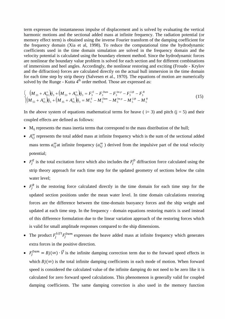
term expresses the instantaneous impulse of displacement and is solved by evaluating the vertical harmonic motions and the sectional added mass at infinite frequency. The radiation potential (or memory effect term) is obtained using the inverse Fourier transform of the damping coefficient for the frequency domain (Xia et al, 1998). To reduce the computational time the hydrodynamic coefficients used in the time domain simulation are solved in the frequency domain and the velocity potential is calculated using the boundary element method. Since the hydrodynamic forces are nonlinear the boundary value problem is solved for each section and for different combinations of immersions and heel angles. Accordingly, the nonlinear restoring and exciting (Froude - Krylov and the diffraction) forces are calculated directly on the actual hull immersion in the time domain for each time step by strip theory (Salvesen et al., 1970). The equations of motion are numerically solved by the Runge - Kutta 4th order method. Those are expressed as:

( ) ( )( ) ( )

−−−−=+++−−−−=+++

∞∞

∞∞

RLiftpDamE

RLiftpDamE

MMMMMAMAMFFFFFAMAM

55Im5553353555555

33Im

3335535333333

ηηηη

(15)

In the above system of equations mathematical terms for heave ( i= 3) and pitch (j = 5) and their

coupled effects are defined as follows:

• Mij represents the mass inertia terms that correspond to the mass distribution of the hull;

• 𝐴𝑖𝑖∞ represents the total added mass at infinite frequency which is the sum of the sectional added

mass terms 𝑎𝑖𝑖∞at infinite frequency (𝑎𝑖𝑖∞ ) derived from the impulsive part of the total velocity

potential;

• 𝐹𝑖𝐸 is the total excitation force which also includes the 𝐹𝑖𝐷 diffraction force calculated using the

strip theory approach for each time step for the updated geometry of sections below the calm

water level;

• 𝐹𝑖𝑅 is the restoring force calculated directly in the time domain for each time step for the

updated section positions under the mean water level. In time domain calculations restoring

forces are the difference between the time-domain buoyancy forces and the ship weight and

updated at each time step. In the frequency - domain equations restoring matrix is used instead

of this difference formulation due to the linear variation approach of the restoring forces which

is valid for small amplitude responses compared to the ship dimensions.

• The product 𝐹𝑖𝐿𝑖𝐿𝐿𝐹𝑖𝐷𝐷𝐷 expresses the heave added mass at infinite frequency which generates

extra forces in the positive direction.

• 𝐹𝑖𝐷𝐷𝐷 = 𝐵𝐵(∞) ∙ 𝑉�⃗ is the infinite damping correction term due to the forward speed effects in

which 𝐵𝐵(∞) is the total infinite damping coefficients in each mode of motion. When forward

speed is considered the calculated value of the infinite damping do not need to be zero like it is

calculated for zero forward speed calculations. This phenomenon is generally valid for coupled

damping coefficients. The same damping correction is also used in the memory function

derivation in order to be sure the infinite value of the corrected damping curve approaches to

zero.

• 𝐹𝑖𝐼𝐷𝐼 = ∬ �∫ 𝜒𝑖(𝑥,𝑦, 𝑧; 𝑡 − 𝜏)𝑉𝑖(𝑥, 𝜏)𝑑𝜏𝐿

−∞ � 𝑑𝑑 = ∫ 𝐾𝑖𝑖(𝑥; 𝑡 − 𝜏)𝑉𝑖(𝑥, 𝜏)𝑑𝜏𝐿−∞𝑆𝐻

for 𝐾𝑖𝑖(𝑡) = 2𝜋 ∫ �𝐵𝑖𝑖(𝜔) − 𝐵𝑖𝑖(∞)� cos (𝜔𝑡)𝑑𝜔∞

0

where 𝐵𝑖𝑖(𝜔) is the sectional frequency domain damping coefficient and V represents the forward

speed.

• 𝐹𝑖𝑅 is the restoring force calculated directly in the time domain for each time step for the updated section positions under the mean water level. In time domain calculations restoring forces are the difference between the time-domain buoyancy forces and the ship weight and updated at each time step. In the frequency-domain equations restoring matrix is used instead of this difference formulation due to the linear variation approach of the restoring forces which is valid for small amplitude responses compared to the ship dimensions.

The hydrodynamic forces are related to the frequency domain using an inverse direct Fourier transform for the actual hull shape and for the calm water level at each time step. Forward speed is modelled with using the approximated forward speed formulations introduced by Mortola et al (2011a). 4. Description of reference conditions Key information on the 10,000 TEU Container Ship used for the current study is given on Figure 3. The experimental results used to benchmark against the methods described in section 3 resulted from the WILS II JIP (Wave Induced Loads on Ships Joint Industry Project II) carried out by the Korean Maritime Research Institute of Ships and Ocean Engineering (KRISO), Lloyd's Register and other major Classification Societies (e.g. see Hong et al., 2010 and Lee at al., 2012). In this paper symmetric motion amplitude operators and corresponding dynamic loads were compared in way of 0.2 rad/s and 1.2 rad/sec for 5 knots and 20 knots forward speed in head (χ = 1800) and quartering (χ = 1500) regular waves of unit amplitude. A summary of the specifics of numerical idealisations is provided in Table 2. It is noted that for the PNL weakly nonlinear idealisation simulations were run for at least 25 periods (see Ballard et al., 2003). On the other hand, for LAMP simulations were run for 20 wave periods until steady state and repeatable responses were obtained (see Mortola et al., 2011). This approach ensured a sufficient length of steady state responses and hence consistency and accuracy in the evaluation of the RAOs.

(a) (b)

LOA (m) 336.64 LBP (m) 321 Breadth (m) 48.4 Height (m) 27.2 Draft (m) 15 Displacement (t) 143741.92 LCG from AP (m) 152.495

(c)

Segment Mass (t) LCG (m) from AP

LCG (x/L) From AP

KG (m) kxx kyy kzz

1 14608.59 26.750 0.08 21.295 17.700 20.000 20.000 2 27488.58 80.250 0.25 21.295 19.800 21.450 21.450 3 36075.10 133.750 0.42 21.295 20.720 23.500 23.500 4 31367.02 185.250 0.58 21.295 19.690 21.200 21.200 5 22386.58 236.550 0.74 21.295 17.510 19.000 19.000 6 11816.03 287.050 0.89 21.295 14.320 18.000 18.000

(d) (e)

Figure 3. Key information for WILS II 10,000 TEU Container Ship (a) general particulars (b) body plan (c) mass distribution of segmented model (d) configuration of model ship setup and locations of sensors – 1/60 scale (e) hydrodynamic testing (NB : kxx, kyy and kzz represent the radii of gyration of roll, pitch and yaw).

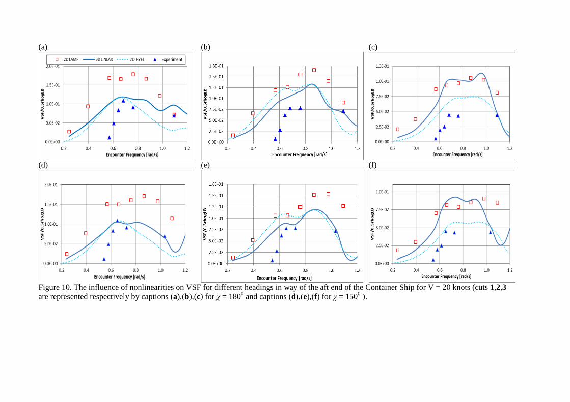
5. Results and discussion The heave and pitch (rad/m) RAOs are shown in Figs. 4 and 5 for 0, 5 and 20 knots forward speeds and headings of 180O and 150O, respectively. Although experimental measurements are only available for 5 and 20 knots, the predictions for zero forward speed are included to compare the predictions only. Predictions are provided by the two-dimensional linear hydroelasticity (2D HYEL), the two-dimensional large amplitude motion (2D LAMP), the three-dimensional linear (3D LINEAR) and the three-dimensional weakly nonlinear (3D PNL) methods. The vertical bending moment (VBM) RAOs for 5 and 20 knots forward speeds and 150O heading are shown in Figs. 6 and 7. The VBM RAOs for 20 knots and headings of 150O and 180O are shown in Figs. 8 and 9. The vertical shear force (VSF) RAOs for 20 knots and headings of 150O and 180O are shown in Figs. 10 and 11. All these figures contain predictions and experimental measurements at

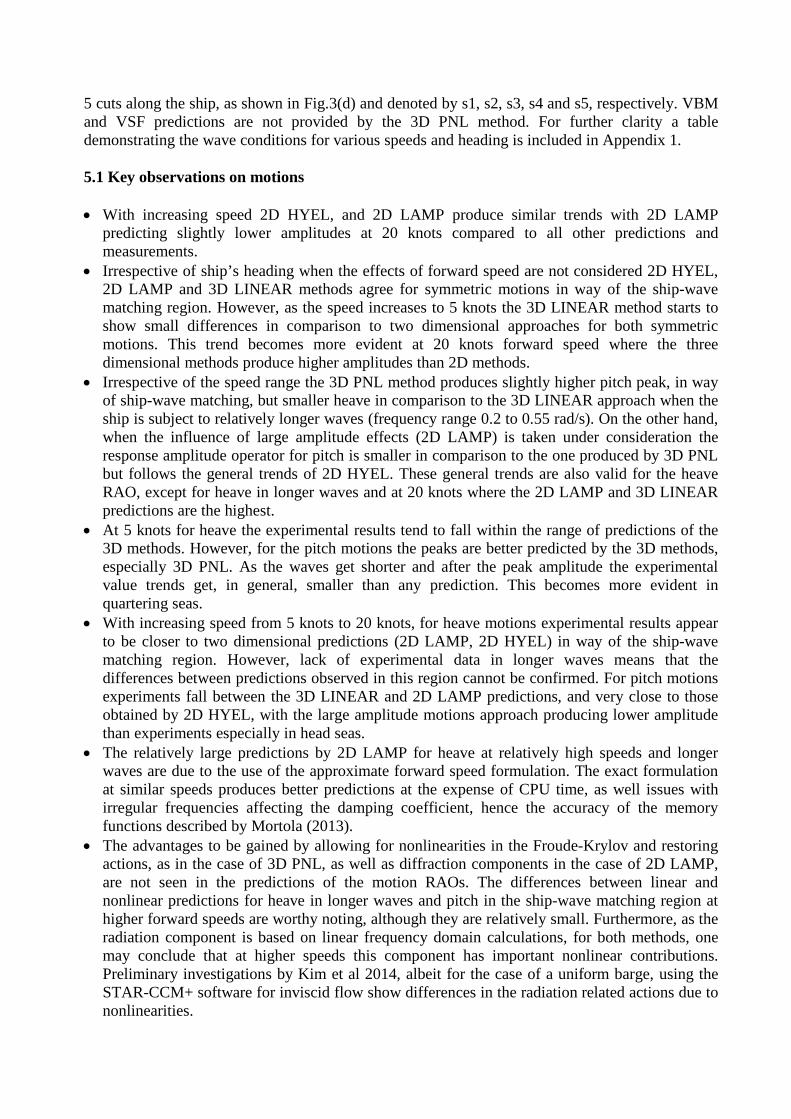
5 cuts along the ship, as shown in Fig.3(d) and denoted by s1, s2, s3, s4 and s5, respectively. VBM and VSF predictions are not provided by the 3D PNL method. For further clarity a table demonstrating the wave conditions for various speeds and heading is included in Appendix 1. 5.1 Key observations on motions • With increasing speed 2D HYEL, and 2D LAMP produce similar trends with 2D LAMP

predicting slightly lower amplitudes at 20 knots compared to all other predictions and measurements.

• Irrespective of ship’s heading when the effects of forward speed are not considered 2D HYEL, 2D LAMP and 3D LINEAR methods agree for symmetric motions in way of the ship-wave matching region. However, as the speed increases to 5 knots the 3D LINEAR method starts to show small differences in comparison to two dimensional approaches for both symmetric motions. This trend becomes more evident at 20 knots forward speed where the three dimensional methods produce higher amplitudes than 2D methods.

• Irrespective of the speed range the 3D PNL method produces slightly higher pitch peak, in way of ship-wave matching, but smaller heave in comparison to the 3D LINEAR approach when the ship is subject to relatively longer waves (frequency range 0.2 to 0.55 rad/s). On the other hand, when the influence of large amplitude effects (2D LAMP) is taken under consideration the response amplitude operator for pitch is smaller in comparison to the one produced by 3D PNL but follows the general trends of 2D HYEL. These general trends are also valid for the heave RAO, except for heave in longer waves and at 20 knots where the 2D LAMP and 3D LINEAR predictions are the highest.

• At 5 knots for heave the experimental results tend to fall within the range of predictions of the 3D methods. However, for the pitch motions the peaks are better predicted by the 3D methods, especially 3D PNL. As the waves get shorter and after the peak amplitude the experimental value trends get, in general, smaller than any prediction. This becomes more evident in quartering seas.

• With increasing speed from 5 knots to 20 knots, for heave motions experimental results appear to be closer to two dimensional predictions (2D LAMP, 2D HYEL) in way of the ship-wave matching region. However, lack of experimental data in longer waves means that the differences between predictions observed in this region cannot be confirmed. For pitch motions experiments fall between the 3D LINEAR and 2D LAMP predictions, and very close to those obtained by 2D HYEL, with the large amplitude motions approach producing lower amplitude than experiments especially in head seas.

• The relatively large predictions by 2D LAMP for heave at relatively high speeds and longer waves are due to the use of the approximate forward speed formulation. The exact formulation at similar speeds produces better predictions at the expense of CPU time, as well issues with irregular frequencies affecting the damping coefficient, hence the accuracy of the memory functions described by Mortola (2013).

• The advantages to be gained by allowing for nonlinearities in the Froude-Krylov and restoring actions, as in the case of 3D PNL, as well as diffraction components in the case of 2D LAMP, are not seen in the predictions of the motion RAOs. The differences between linear and nonlinear predictions for heave in longer waves and pitch in the ship-wave matching region at higher forward speeds are worthy noting, although they are relatively small. Furthermore, as the radiation component is based on linear frequency domain calculations, for both methods, one may conclude that at higher speeds this component has important nonlinear contributions. Preliminary investigations by Kim et al 2014, albeit for the case of a uniform barge, using the STAR-CCM+ software for inviscid flow show differences in the radiation related actions due to nonlinearities.

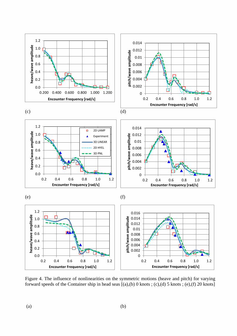
5.2 Key observations on Vertical Bending Moments & Shear forces • By examining Figs.6 and 7, for 5 knots, it can be seen that, by and large, VBM predictions by

2D HYEL and 3D LINEAR methods are close, and lower than the 2D LAMP results in way of the after half of the ship (cuts 1 and 2). On the other hand in way of the forward half of the ship 2D LAMP and 2D HYEL predictions become closer and, in general, higher than 3D LINEAR. All three predictions are close in the vicinity of amidships (cut 3). The same trends are also valid for the predictions at the higher speed of 20 knots, also shown in Figs. 6 and 7. These trends are also valid for the predictions shown in Figs. 8 and 9, for the ship travelling at 20 knots in regular head waves.

• For 150O heading, experimental VBMs are, in general, lower than those produced by 2D LAMP in way of the aft half of the ship (cuts 1 and 2). The convergence between 2D LAMP and experimental measurements is improving from amidships (cut 3) and toward forward quarter of the hull (cut 4). In general the predictions by 2D HYEL are closer to the experimental measurements. The foremost position (cut 5) shows the largest difference between experiments and predictions, with the latter smaller than the measured loads.

• When considering the VBM RAOs in head waves (see Figs. 8a,b,c and 9a,b), the experimental measurements display a trend with frequency which is different than all predictions. Experimentally derived loads reduce in magnitude around 0.6 rad/s, and for all cuts are lower than any predicted VBM. The linear predictions, especially 3D LINEAR provide the best agreement with the experimental bending moment, except for that in way of cut 5.

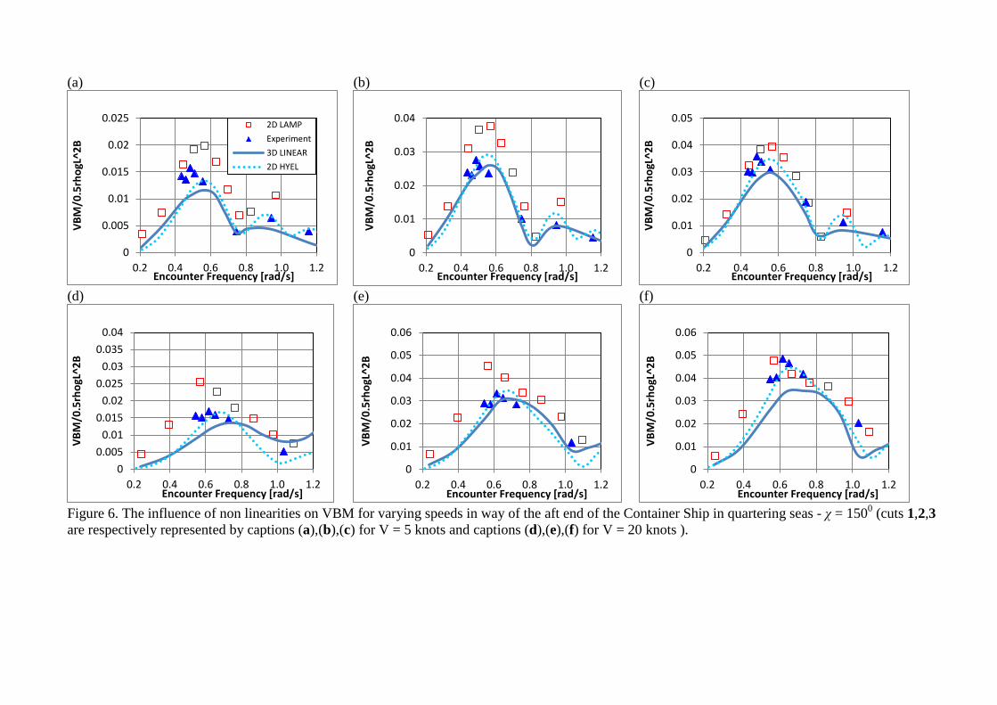
• It is difficult to identify specific trends for the VSF RAOs at 20 knots (see Figs. 10 and 11). The linear predictions, 2D HYEL and 3D LINEAR, are close in cuts 1,2 and 4, but 3D LINEAR predictions are larger than 2D HYEL in cuts 3 and 5. On the other hand, 2D LAMP predictions are achieve their largest peak in way of the aft part of the hull and appear to be equally as large as those provided by 3D LINEAR in way of amidships. In the forward part (cuts 4,5) 2D LAMP predictions are close to those by 2D HYEL. These observations are valid for both headings shown in Figs. 10 and 11. Bennett et al (2013 and 2014) also noted similar type of large differences between experimental VBM RAOs and predictions at the fore and aft quarter lengths compared to amidships for the case of a typical naval frigate.

• When comparing experimental and predicted VSF RAOs one notes, again, the lack of trends. In general, the experimental VSF are lower or close to 2D HYEL, except in way of cut 4 where 2D LAMP seems to provide the closest matching.

• Troughout the benchmark it becomes evident that the relative differences between different prediction methods, in general, do not appear to be significantly affected by forward speed. This is also confirmed by the zero speed predictions for VBM and VSF, which are not shown here.

(a) (b)

(c) (d)

(e) (f)

Figure 4. The influence of nonlinearities on the symmetric motions (heave and pitch) for varying forward speeds of the Container ship in head seas [(a),(b) 0 knots ; (c),(d) 5 knots ; (e),(f) 20 knots] (a) (b)

0.0

0.2

0.4

0.6

0.8

1.0

1.2

0.200 0.400 0.600 0.800 1.000 1.200

heav

e/w

ave

ampl

itude

Encounter Frequency [rad/s] 0

0.002

0.004

0.006

0.008

0.01

0.012

0.014

0.2 0.4 0.6 0.8 1.0 1.2

pitc

h/w

ave

ampl

itude

Encounter Frequency [rad/s]

0.0

0.2

0.4

0.6

0.8

1.0

1.2

0.2 0.4 0.6 0.8 1.0 1.2

heav

e/w

ave

ampl

itude

Encounter Frequency [rad/s]

2D LAMP

Experiment

3D LINEAR

2D HYEL

3D PNL

0

0.002

0.004

0.006

0.008

0.01

0.012

0.014

0.2 0.4 0.6 0.8 1.0 1.2

pitc

h/w

ave

ampl

itude

Encounter Frequency [rad/s]

0.0

0.2

0.4

0.6

0.8

1.0

1.2

0.2 0.4 0.6 0.8 1.0 1.2

heav

e/w

ave

ampl

itude

Encounter Frequency [rad/s]

00.0020.0040.0060.008

0.010.0120.0140.016

0.2 0.4 0.6 0.8 1.0 1.2

pitc

h/w

ave

ampl

itude

Encounter Frequency [rad/s]

(c) (d)

(e) (f)

Figure 5. The influence of nonlinearities on the symmetric motions (heave and pitch) for varying speeds of the Container ship in oblique seas (χ = 1500) [(a),(b) 0 knots ; (c),(d) 5 knots ; (e),(f) 20 knots]

0.0

0.2

0.4

0.6

0.8

1.0

1.2

0.2 0.4 0.6 0.8 1.0 1.2

heav

e/w

ave

ampl

itude

Encounter Frequency [rad/s]

0

0.002

0.004

0.006

0.008

0.01

0.012

0.014

0.2 0.4 0.6 0.8 1.0 1.2

pitc

h/w

ave

ampl

itude

Encounter Frequency [rad/s]

0.0

0.2

0.4

0.6

0.8

1.0

1.2

0.2 0.4 0.6 0.8 1.0 1.2

heav

e/w

ave

ampl

itude

Encounter Frequency [rad/s]

2D LAMP

Experiment

3D LINEAR

2D HYEL

3D PNL

00.0020.0040.0060.008

0.010.0120.014

0.2 0.4 0.6 0.8 1.0 1.2

pitc

h/w

ave

ampl

itude

Encounter Frequency [rad/s]

0.0

0.2

0.4

0.6

0.8

1.0

1.2

0.2 0.4 0.6 0.8 1.0 1.2

heav

e/w

ave

ampl

itude

Encounter Frequency [rad/s] 0

0.005

0.01

0.015

0.02

0.2 0.4 0.6 0.8 1.0 1.2

pitc

h/w

ave

ampl

itude

Encounter Frequency [rad/s]

(a) (b) (c)

(d) (e) (f)

Figure 6. The influence of non linearities on VBM for varying speeds in way of the aft end of the Container Ship in quartering seas - χ = 1500 (cuts 1,2,3 are respectively represented by captions (a),(b),(c) for V = 5 knots and captions (d),(e),(f) for V = 20 knots ).

0

0.005

0.01

0.015

0.02

0.025

0.2 0.4 0.6 0.8 1.0 1.2

VBM

/0.5

rhog

L^2B

Encounter Frequency [rad/s]

2D LAMPExperiment3D LINEAR2D HYEL

0

0.01

0.02

0.03

0.04

0.2 0.4 0.6 0.8 1.0 1.2

VBM

/0.5

rhog

L^2B

Encounter Frequency [rad/s]

0

0.01

0.02

0.03

0.04

0.05

0.2 0.4 0.6 0.8 1.0 1.2

VBM

/0.5

rhog

L^2B

Encounter Frequency [rad/s]

00.005

0.010.015

0.020.025

0.030.035

0.04

0.2 0.4 0.6 0.8 1.0 1.2

VBM

/0.5

rhog

L^2B

Encounter Frequency [rad/s]

0

0.01

0.02

0.03

0.04

0.05

0.06

0.2 0.4 0.6 0.8 1.0 1.2

VBM

/0.5

rhog

L^2B

Encounter Frequency [rad/s]

0

0.01

0.02

0.03

0.04

0.05

0.06

0.2 0.4 0.6 0.8 1.0 1.2

VBM

/0.5

rhog

L^2B

Encounter Frequency [rad/s]

(a) (b)

(c) (d)

Figure 7. The influence of nonlinearities on VBM for varying forward speeds in way of the forward end of the Container Ship in quartering seas - χ = 1500 (cuts 4,5 are respectively represented by captions (a),(b) for V = 5 knots and captions (c),(d) for V = 20 knots ).

0

0.005

0.01

0.015

0.02

0.025

0.2 0.4 0.6 0.8 1.0 1.2

VBM

/0.5

rhog

L^2B

Encounter Frequency [rad/s]

2D LAMPExperiment3D LINEAR2D HYEL

0

0.001

0.002

0.003

0.004

0.005

0.006

0.2 0.4 0.6 0.8 1.0 1.2

VBM

/0.5

rhog

L^2B

Encounter Frequency [rad/s]

0

0.005

0.01

0.015

0.02

0.025

0.03

0.035

0.2 0.4 0.6 0.8 1.0 1.2

VBM

/0.5

rhog

L^2B

Encounter Frequency [rad/s]

00.0010.0020.0030.0040.0050.0060.0070.0080.009

0.010.011

0.2 0.4 0.6 0.8 1.0 1.2

VBM

/0.5

rhog

L^2B

Encounter Frequency [rad/s]

(a) (b) (c)

(d) (e) (f)

Figure 8. The influence of nonlinearities on VBM for varying headings in way of the aft end of the Container Ship for V = 20 knots (cuts 1,2,3 are represented respectively by captions (a),(b),(c) for χ = 1800 and captions (d),(e),(f) for χ = 1500 ).

0.0E+00

5.0E-03

1.0E-02

1.5E-02

2.0E-02

2.5E-02

3.0E-02

0.20 0.40 0.60 0.80 1.00 1.20

VBM

/0.5

rhog

L^2B

Encounter Frequency [rad/s]

3D LINEAR2D HYEL2D LAMPExperiment

(a) (b)

(c) (d)

Figure 9. The influence of nonlinearities on VBM for varying headings in way of the forward end of the Container Ship for V = 20 knots (cuts 4,5 are represented respectively by captions (a),(b) for χ = 1800 and captions (c),(d) for χ = 1500 ).

0.0E+00

5.0E-03

1.0E-02

1.5E-02

2.0E-02

2.5E-02

3.0E-02

3.5E-02

0.200 0.400 0.600 0.800 1.000 1.200

VBM

/0.5

rhog

L^2B

Encounter Frequency [rad/s]

0.0E+001.0E-032.0E-033.0E-034.0E-035.0E-036.0E-037.0E-038.0E-039.0E-031.0E-021.1E-02

0.200 0.400 0.600 0.800 1.000 1.200

VBM

/0.5

rhog

L^2B

Encounter Frequency [rad/s]

(a) (b) (c)

(d) (e) (f)

Figure 10. The influence of nonlinearities on VSF for different headings in way of the aft end of the Container Ship for V = 20 knots (cuts 1,2,3 are represented respectively by captions (a),(b),(c) for χ = 1800 and captions (d),(e),(f) for χ = 1500 ).

(a) (b)

(c) (d)

Figure 11. The influence of nonlinearities on VSF for different headings in way of the forward end of the Container Ship for V = 20 Knots (cuts 4,5 are represented respectively by captions (a),(b) for χ = 1800 and captions (c),(d) for χ = 1500 ).

6. Conclusions

In this paper fluid structure interaction models with varying degrees of complexity were assessed against available experimental results for a 10,000 TEU container ship. Comparisons focused on symmetric motions and loads in regular waves for two different speeds and headings. It was shown that both linear and partly nonlinear methods provide practically good predictions for pitch and with a few exceptions, e.g. longer waves, for heave. However, it is difficult to identify one method, and one set of assumptions, providing equally good predictions for all of the operational conditions considered. For the VBMs differences between predictions and measurements vary depending mainly, on position, but also heading. Notwithstanding for the case of the VBM in way of amidships the agreement between predictions and experiments is practically good, except for head waves. The majority of experimental, and indeed full-scale measurements, tend to focus on amidships (e.g. Hirdaris et al, 2011 and Bennett, 2014). In furthering this work our investigations indicate that one is likely to come across interesting differences at locations away from amidships; hence, it is recommended that segmented model experiments should be designed so as to be suitable for measurements between 0.2 and 0.8 of the ships' length (for example see Peng et al., 2014). Future research may consider the effects of nonlinear waves and associated model tests for validation. The apparent difficulties in providing accurate load predictions towards the fore and aft ends of the hull are also confirmed by the VSF results. This work indicates that accounting for nonlinear effects is important, but accounting only for some nonlinear influences may not necessarily improve the accuracy of the prediction. Accordingly, weakly non-linear methods may, yet, be proved reliable tools for predicting the wave-induced loads and responses of a ship in waves provided that hydrodynamic assumptions and their respective influence on wave induced motions and loads are well understood and validated. Furthermore, the validity of modelling assumptions related with linear radiation and diffraction forces, particularly when there are noticeable variations of the hull wetted surface in time, should be carefully considered when using weakly nonlinear hydrodynamic approaches for predicting ship response. 6. Acknowledgements The results and opinions presented in this publication do not necessary express the views of the corporate organisations represented by the authors. Individual authors acknowledge the support from technical colleagues within their own organisations and funding provided via the Lloyd's Register Strategic Research programme on Ship Hydrodynamics. Special thanks of appreciation go to the Korean Research Institute of Ships and Ocean Engineering (KRISO) and WILS II Joint Industry Project partners for the use of the experimental results presented in this paper. Dr. G. Mortola acknowledges that the results on large amplitude motions presented in this paper originate from his PhD work at the University of Strathclyde, Glasgow (UK). Dr. Spyros Hirdaris completed this paper while working at Lloyd’s Register’s Marine New Construction Offices at Hyundai Heavy Industries (Ulsan, South Korea). He therefore acknowledges the support received by the Lloyd’s Register Asia local management team. ''Lloyd’s Register, its affiliates and subsidiaries and their respective officers, employees or agents are, individually and collectively, referred to in this clause as the ‘‘Lloyd’s Register Group Ltd’’. The Lloyd’s Register Group Ltd. assumes no responsibility and shall not be liable to any person for any loss, damage or expense caused by reliance on the information or advice in this document or howsoever provided, unless that person has signed a contract with the relevant Lloyd’s Register Group Ltd. entity for the provision of this information or advice and that in this case any responsibility or liability is exclusively on the terms and conditions set out in that contract.'' 7. References

Ba, M., Guilband, M. (1995). A fast method of evaluation for the transient and pulsating Green’s function. Schiffstechnik – Ship Technology Research, 42:68-80. Ballard, E.J., Hudson, D.A., Price, W.G., and Temarel, P. (2003). Time Domain Simulation of Symmetric Ship Motions in Waves. Transactions of the Royal Institution of Naval Architects, 145:1-20. Bailey, P.A., Price, W.G., and Temarel, P. (1997). A Unified Mathematical Model Describing the Manoeuvring of a Ship Travelling in a Seaway. Transactions of the Royal Institution of Naval Architects, 139:131-149. Bailey, P.A., Hudson, D.A., Price, W.G., and Temarel, P. (2002a). Time Simulation of Manoeuvring and Seakeeping Assessments Using a Unified Mathematical Model. Transactions of the Royal Institution of Naval Architects, 144:57-78. Bailey, P.A., Hudson, D.A., Price, W.G., and Temarel, P. (2002b). A Simple yet Rational Approach to Panelling of Hull Surfaces. Transactions of the Royal Institution of Naval Architects, 144:79-91. Bennett, S.S, Hudson, D.A., Temarel, P. (2013). The influence of forward speed on ship motions in abnormal waves: Experimental measurements and numerical predictions. Journal of Fluids and Structures, 39:154-172. Bennett, S.S, Hudson, D.A., Temarel, P. (2014). Global wave-induced loads in abnormal waves: Comparison between Experimental Results and Classification Society Rules. Journal of Fluids and Structures, 49:498-515. Bishop, R.E.D. and Price, W.G. (1979). Hydroelasticity of Ships, ISBN 0-521-22328-8, Published in the UK by Cambridge University Press. Chapchap, A., Hudson, D.A., Temarel, P., Ahmed, T.M., Hirdaris, S.E. (2011). The influence of forward speed and nonlinearities on the dynamic behaviour of a container ship in regular waves. Transactions of the Royal Institution of Naval Architects Part A: International Journal of Maritime Engineering, 153(2)137-148. Cummins, W.E. (1962). The Impulse Response Function and Ship Motions, Schiffstechnik, 9: 101-109. Du, S.X., Hudson, D.A., Price, W.G., and Temarel, P. (2009). Implicit Expressions of Static and Incident Wave Pressures over the Instantaneous Wetted Surface of Ships, Proceedings of the Institution of Mechanical Engineers Part M: Journal of Engineering for the Maritime Environment, 223 (3):239-256. Fonseca, N and Guedes Soares, C. (2002). Comparison of Numerical and Experimental Results of Nonlinear Wave-induced Vertical Ship Motions and Loads. Journal of Marine Science and Technology 6(4):193-204.

Hanninen, S.K., Mikkola, T. & Matusiak, J. (2012). On the numerical accuracy of the wave load distribution on a ship advancing in short and steep waves. Journal of Marine Science and Technology 17(2): 125-138.

Hirdaris, S.E. Bai, W., Dessi, D., Ergin, A., Gu, X., Hermundstad, O.A., Huijsmans, R., Iijima, K., Nielsen, U.D., Parunov, J., Fonseca, N., Papanikolaou, A., Argyriadis, K., Incecik, A. (2014). Loads for use in the design of ships and offshore structures. Ocean Engineering, 78:131-174. Hirdaris, S.E., White, N., Angoshtari, N., Johnson, M.C., Lee, Y.N. Bakkers, N. (2011). Wave Loads and Flexible Fluid Structure Interactions - Present Developments and Future Directions. Ships and Offshore Structures, 5(4):307-325.

Hirdaris, S.E. and Temarel, P. (2009). Hydroelasticity of Ships: Recent Advances and Future trends. Proceedings of the Institution of Mechanical Engineers Part M: Journal of Engineering for the Maritime Environment, Special Issue on Fluid Structure Interactions in Honour of W.G. Price, 223(3):305-330. Hong, S.Y., Kim, B.W., Kim, J.H., Sung, H.G., Kim, Y.S., Cho, S.K., Nam, B.W., Choi, S.K., Lee, C.Y., Lim, D.W., and Kwon, M.K. (2010). Wave Induced Loads on Ships 2nd Joint Industry Project (WILS II JIP) Final Report, MOERI Tech Report No. BSPIS503A-2207-2. Inglis, R.B., and Price, W.G. (1981). Calculation of the Velocity Potential of a Translating- Pulsating Source. Transactions of the Royal Institution of Naval Architects, 123:163-175. Kim, J.H., Lakshmynarayanana, P.A. and Temarel, P. (2014). Added Mass and Damping Coefficients for a Uniform Flexible Barge Using VOF, In Proceedings of the 11th International Conference on Hydrodynamics (ICHD 2014), 19th to 24th October 2014, Singapore, ISBN 978-981-09-2175-0. Lakshmynarayanana, P.A., Temarel, P. and Chen, Z. (2015). Hydroelastic Analysis of a Flexible Barge in Regular Waves Using Coupled CFD-FEM Modelling, In Proceedings of the 5th International Conference on Marine Structures, MARSTRUCT '15, Southampton, UK (in press). Lee, Y., White, N., Wang, Z., Hirdaris, S.E. and Zhang, S. (2012). Comparison of Springing and Whipping Responses of Model Tests with Predicted Nonlinear Hydroelastic Analyses. The International Journal of Offshore and Polar Engineering IJOPE, 22 (3):1-8, ISSN 1053-5381. Mortola, G. (2013). Nonlinear Analysis of Waves Induced Motions and Loads in Large Amplitude Waves, PhD Thesis, pp. 167, Department of Naval Architecture and Marine Engineering, The University of Strathclyde, Glasgow, UK. Mortola, G., Incecik, A., Turan, O., and Hirdaris, S.E. (2011a). Nonlinear Analysis of Ship Motions and Loads in Large Amplitude Waves. Transactions of the Royal Institution of Naval Architects, 153(2):81-87. Mortola, G., Incecik, A., Turan O., and Hirdaris, S. (2011b). A Nonlinear Approach to the Calculation of Large Amplitude Motions and Wave Loads, Proceedings of the XIV Congress of the International Maritime Association of the Mediterranean, Genoa, Italy 12-16 September 2011. Oberhagemann, J., Shigunov, V. and El Moctar, O. (2012). Application of CFD in Long-term Extreme Value Analyses of Wave Loads. Schiffstechnik – Ship Technology Research, 59(3): 4-22. Peng, S., Temarel, P., Bennett, S.S., Wu, W., Lin, Z., Wang, Y. (2014). Symmetric response of a hydroelastic scaled container ship model in regular and irregular waves. Proceedings of the ASME

33rd International Conference on Ocean, Offshore and Arctic Engineering OMAE2014-23860, June 8 – 13, San Fransisco, California, USA. Rathje, H., Schellin, T.E. and Brehm, A. (2011). Speed Loss in Waves and Wave-Induced Torsion of a Wide-breadth Containership. Proceedings of the Institution of Mechanical Engineers, Part M: Journal of Engineering for the Maritime Environment, 225:387-401. Sclavounos, P.D. and Lee, C.H. (1985). Topics on Boundary Element Solutions of Wave Radiation Diffraction Problems. Proceedings of the 4th International Conference on Numerical Ship Hydrodynamics, Edited by Justin H. McCarthy – National Academy of Sciences, Washington D.C, USA. ISSC (2009). Report of the ISSC Technical Committee I.2 on Loads, 1:127-210. 17th International Ship and offshore Structures Congress (ISSC), ISBN: 9788995 473016, Seoul, South Korea. Quérard, A.B.G., Temarel, P. and Turnock, S.R. (2010). Application of RANS to hydrodynamics of Bilge Keels and Baffles. In Proceedings of the William Froude Conference on Advances in Theoretical and Applied Hydrodynamics – Past and Future, Portsmouth, UK. Salvesen, N., Tuck, E.O. and Faltisen, O. (1970). Ship Motions and Sea Loads. Transactions of the Society of Naval Architects and Marine Engineers, 78:250-287. Temarel, P. and Hirdaris S.E. Eds. (2009). Proceedings of the 5th International Conference on Hydroelasticity in Marine Technology (HYELAS '09), Published by the University of Southampton, HIghfiled, Southampton, UK, ISBN: 9780854329045. Xia, J., Wang, Z. and Jensen, J.J. (1998). Nonlinear Wave Loads and Ship Responses by a Time Domain Strip Theory, Marine Structures, 11:101-123.

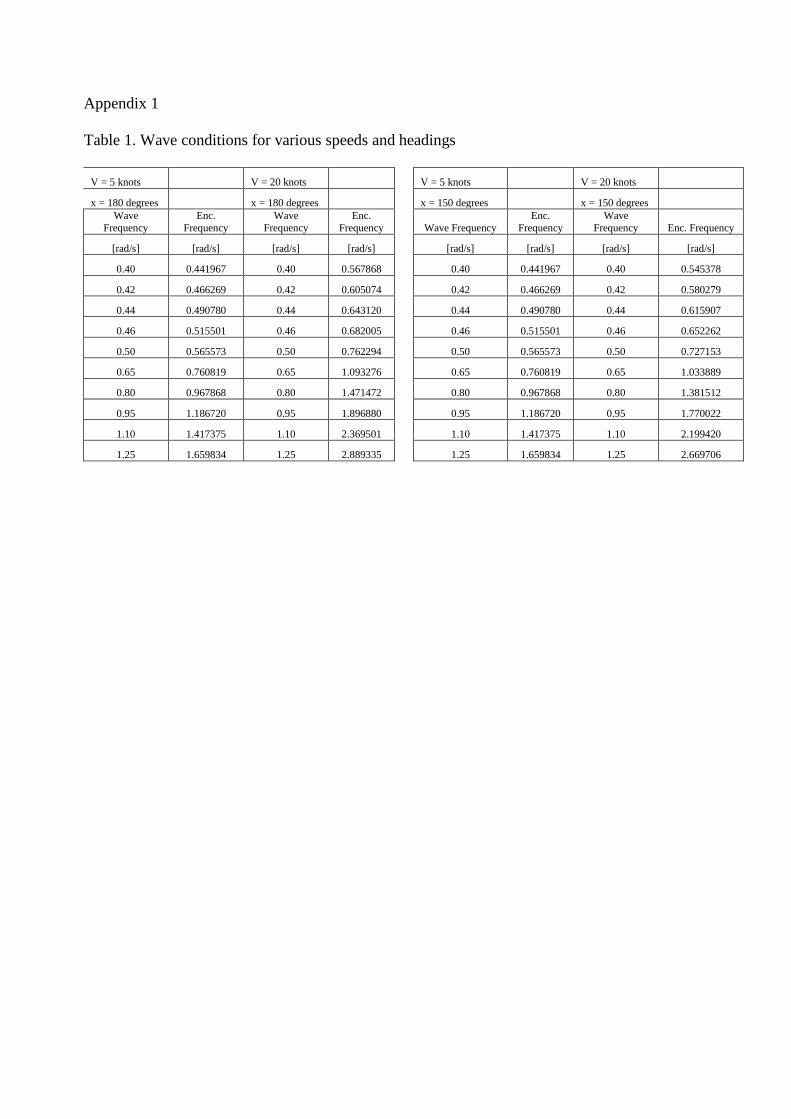
Appendix 1 Table 1. Wave conditions for various speeds and headings

V = 5 knots V = 20 knots

V = 5 knots V = 20 knots

x = 180 degrees x = 180 degrees

x = 150 degrees x = 150 degrees

Wave Frequency

Enc. Frequency

Wave Frequency

Enc. Frequency

Wave Frequency

Enc. Frequency

Wave Frequency Enc. Frequency

[rad/s] [rad/s] [rad/s] [rad/s]

[rad/s] [rad/s] [rad/s] [rad/s]

0.40 0.441967 0.40 0.567868

0.40 0.441967 0.40 0.545378

0.42 0.466269 0.42 0.605074

0.42 0.466269 0.42 0.580279

0.44 0.490780 0.44 0.643120

0.44 0.490780 0.44 0.615907

0.46 0.515501 0.46 0.682005

0.46 0.515501 0.46 0.652262

0.50 0.565573 0.50 0.762294

0.50 0.565573 0.50 0.727153

0.65 0.760819 0.65 1.093276

0.65 0.760819 0.65 1.033889

0.80 0.967868 0.80 1.471472

0.80 0.967868 0.80 1.381512

0.95 1.186720 0.95 1.896880

0.95 1.186720 0.95 1.770022

1.10 1.417375 1.10 2.369501

1.10 1.417375 1.10 2.199420

1.25 1.659834 1.25 2.889335

1.25 1.659834 1.25 2.669706