the influence of mean stress in the design with hfmi-treated
TRANSCRIPT
DEPARTMENT OF ARCHITECTURE AND CIVIL ENGINEERING DIVISION OF STRUCTURAL ENGINEERING
CHALMERS UNIVERSITY OF TECHNOLOGY Gothenburg, Sweden 2020
www.chalmers.se
The influence of mean stress in the design with HFMI-treated welds Investigation of design models to the Eurocode Master’s Thesis in the Masters’s Programme Structural Engineering and Building Technology
JOHAN NILSSON

DEPARTMENT OF ARCHITECHTURE AND CIVIL ENGINEERING
DIVISION OF STRUCTURAL ENGINEERING CHALMERS UNIVERSITY OF THNOLOGY
Gothenburg, Sweden
www.clmers.se
MASTER’S THESIS ACEX30
The influence of mean stress in the design of bridges with
HFMI-treated welds
Investigation of design models to the Eurocode
Master’s Thesis in the Master’s Programme Structural Engineering and Building Technology
JOHAN NILSSON
Department of Architecture and Civil Engineering
Division of Structural Engineering
Lightweight Structures
CHALMERS UNIVERSITY OF TECHNOLOGY
Göteborg, Sweden 2020


I
The influence of mean stress in the design of bridges with HFMI-treated welds
Investigation of design models to the Eurocode
Master’s Thesis in the Master’s Programme Structural Engineering and Building
Technology
JOHAN NILSSON
© JOHAN NILSSON, 2020
Examensarbete ACEX30
Institutionen för arkitektur och samhällsbyggnadsteknik
Chalmers tekniska högskola, 2020
Department of Architecture and Civil Engineering
Division of Division Name
Research Group Name
Chalmers University of Technology
SE-412 96 Göteborg
Sweden
Telephone: + 46 (0)31-772 1000
Chalmers Reproservice / Department of Architecture and Civil Engineering
Göteborg, Sweden, 2020


I
The influence of mean stress in the design of bridges with HFMI-treated welds
Investigation of design models to the Eurocode
Master’s thesis in the Master’s Programme Master’s Structural Engineering and
Building Technology
JOHAN NILSSON
Department of Architecture and Civil Engineering
Division of Structural Engineering
Lightweight Structures
Chalmers University of Technology
ABSTRACT
High-frequency mechanical impact (HFMI) is a post-weld treatment method to increase
the fatigue strength of welded components. Most of the research on the performance of
HFMI-treated joints has been carried out on structures subjected to constant amplitude
loading. However, traffic loads on bridges can generate high and varying mean stresses,
which are effects that are not covered by any design recommendations based on these
earlier researches. A recent published report suggests a design framework that allows
bridge designers to include the effect of mean stress under variable amplitude loading,
without information about the stress range spectrum. In this work, traffic simulations
are performed to investigate the validity of the suggested design framework, showing
that the same results are obtained even for an increased traffic data pool. The same
simulations are carried out on Dutch traffic, revealing that the design framework is
applicable to traffic situations in other countries than Sweden. Finally, an alternative
design framework is developed and presented.
Key words: fatigue; bridge; HFMI, variable amplitude; mean stress; design

CHALMERS, Architecture and Civil Engineering, Master’s Thesis ACEX30 II
Contents
ABSTRACT I
CONTENTS II
PREFACE V
NOTATIONS VI
1 INTRODUCTION 1
1.1 Background 1
1.2 Aim and objectives 1
1.3 Methodology 2
1.4 Limitations 3
2 FATIGUE DESIGN OF STEEL AND COMPOSITE BRIDGES 4
2.1 Fatigue load models in Eurocode 4 2.1.1 Fatigue load model 1 4
2.1.2 Fatigue load model 2 5 2.1.3 Fatigue load model 3 6
2.1.4 Fatigue load model 4 6 2.1.5 Fatigue load model 5 7
2.2 Fatigue verification methods 7 2.2.1 The λ-coefficient method 8
2.2.2 Palmgren-Miner’s damage accumulation method 8
3 POST WELD TREATMENT (PWT) METHODS 11
3.1 Classification of PWT methods 11 3.1.1 Weld geometry improvement methods 11
3.1.2 Residual stress methods 12
3.2 High Frequency Mechanical Impact (HFMI) 13
3.2.1 Description of the process 13 3.2.2 Influence of loading 13
3.2.3 Design framework 14
4 VALIDITY OF THE TRAFFIC DATA 17
4.1 Increased traffic data pool 17 4.1.1 The Swedish traffic data pool 17
4.1.2 Result 17
4.2 Comparison with Dutch traffic data 18
4.2.1 The Dutch traffic data pool 18 4.2.2 Result 18 4.2.3 Sensitivity of the method to maximum stress range 19
5 IMPROVEMENTS OF THE METHOD 21

CHALMERS Architecture and Civil Engineering, Master’s Thesis ACEX30 III
5.1 New definition of Φ 21
5.1.1 Design framework 22
6 PREDICTION OF 𝜆HFMI USING FATIGUE LOAD MODELS 24
6.1 Results 25
6.1.1 FLM3 25 6.1.2 FLM4 25
7 𝜆HFMI IN CASE-STUDY BRIDGES 29
8 DISCUSSION 32
8.1 Chapter 4 – Validity of the data 32
8.2 Chapter 5 – Improvements of the method 32
8.3 Chapter 6 – Prediction of λHFMI using fatigue load models 32
8.4 Chapter 7 - λHFMI in case-study bridges 34
9 CONCLUSIONS 35
9.1 Suggestions for further research 35
10 REFERENCES 36
APPENDIX A 38

CHALMERS, Architecture and Civil Engineering, Master’s Thesis ACEX30 IV

CHALMERS Architecture and Civil Engineering, Master’s Thesis ACEX30 V
Preface
The work in this Master’s Thesis has been carried out between January and June 2020
at the Division of Structural Engineering at Chalmers University of Technology,
Gothenburg, Sweden.
I would like to express my gratitude to my supervisor Doctor Poja Shams-Hakimi. His
guidelines and supervision have been of great importance to the development of this
thesis. I would also like to thank my examiner Professor Mohammad Al-Emrani for his
professional input and many ideas.
Gothenburg, June 2020
Johan Nilsson

CHALMERS, Architecture and Civil Engineering, Master’s Thesis ACEX30 VI
Notations
AW as-welded
CA constant amplitude
FAT fatigue strength at 2∙106 cycles
HFMI high-frequency mechanical impact
IIW International Institute of Welding
VA variable amplitude
D damage factor
f mean stress correction factor
L span length
m slope of SN curve
N number of cycles to failure
R stress ratio
S nominal stress
Ssw self-weight stress
Δ𝑆𝑒𝑞 Palmgren-Miner’s equivalent stress range
Δ𝑆𝑒𝑞𝑅 equivalent stress range accounting for stress ratio
Δ𝑆𝑚𝑎𝑥 maximum nominal stress range from traffic
Δ𝑆𝑚𝑖𝑛 minimum nominal stress range from traffic
Δ𝑆𝑝 nominal stress range from FLM3
𝜆𝐻𝐹𝑀𝐼 ratio of Δ𝑆𝑒𝑞𝑅 and Δ𝑆𝑒𝑞
Φ ratio of self-weight stress to maximum stress range from traffic
𝜉 ratio of Δ𝑆𝑒𝑞 and Δ𝑆𝑝

CHALMERS Architecture and Civil Engineering, Master’s Thesis ACEX30 VII


CHALMERS Architecture and Civil Engineering, Master’s Thesis ACEX30 1
1 Introduction
1.1 Background
Steel structures exposed to cyclic loading can be expected to end up in a failure which
is caused by initiation and growth of cracks at sensitive locations which over time can
lead to structural failure. This is known as fatigue failure and can take place at
weldments for load levels below the elastic limit of the material. In addition, fatigue
failure can be of brittle nature which can pose a potentially dangerous failure mode in
structures exposed to cyclic loading [1].
In the end of 2010, Sweden devolved from designing bridges according to the national
design codes, i.e. Bro 2004 and BSK 07, to the new European standards Eurocode. The
transition resulted in that fatigue, which according to the old standards rarely ended up
as the decisive failure mode, to instead became a criterion that could dominate the
design of bridge structures. This has caused new steel bridges to require more material
than before, leading to loss of competitiveness compared with other materials [2].
Since the fatigue limit state (FLS) more often governs the design, alternatives to
conventional bridge designs become relevant. Studies have shown that the combination
of high strength steel and post weld treatment can save around 20 % material [3][4].
One of the most efficient post weld treatment techniques is High-Frequency Mechanical
Impact (HFMI) treatment. This treatment improves the fatigue strength at the weld toe
through high-frequency impacts which introduce compressive residual stresses in
fatigue-sensitive locations through plastic deformations. Moreover, the local stress
concentration is reduced due to a smoother transition at the weld toe and minor weld
defects are eliminated [5].
The International Institute of Welding (IIW) [5] provides design guidelines for the
HFMI technique. However, the part of the recommendations concerning the treatment
of the mean stress effect is not applicable for bridges, which are subjected to variable
amplitude (VA) loading. Shams-Hakimi and Al-Emrani [3][6] therefore proposed an
alternative method to account for the mean stress effect which is more suitable for VA
loads. Commonly, during the design of bridges, the designer has no information about
the detailed traffic data and can therefore not predict the characteristics of the VA load.
In order to obtain a usable method for bridge designers, Shams-Hakimi and Al-Emrani
also developed a design framework based on measurements of 55,000 Swedish trucks.
This design framework will be referred to as the λHFMI-method in the followings.
1.2 Aim and objectives
The aim of this thesis is to study realistic load effects in bridges and investigate the
impact of the mean stresses on the performance of HFMI-treated welds. The following
questions defines the objectives of this project.
• To investigate if the 55,000 vehicles, used in the design framework (the λHFMI-
method) by Shams-Hakimi and Al-Emrani, is enough to represent Swedish road
traffic in terms of the mean stress effect.

CHALMERS, Architecture and Civil Engineering, Master’s Thesis ACEX30 2
• To investigate the validity and identify potential improvements of the λHFMI-
method.
• To study if the the λHFMI-method is applicable to traffic in other European
countries.
• To study whether the Eurocodes fatigue load models can be used to predict the
actual mean stress effect in HFMI-treated bridges.
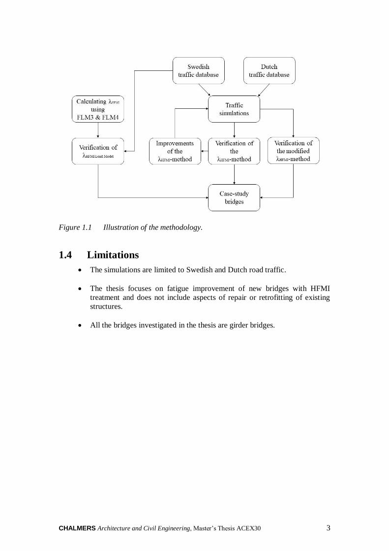
1.3 Methodology
The first step towards fulfilment of the presented aim and objectives consisted of a
literature study. The goal was to provide information about different post weld
treatment techniques, in particular the HFMI technique, and also about the effects that
VA loading has on HFMI-treated welds. The purpose of the literature study was also to
provide information about the design process and fatigue design verification of steel
and composite steel/concrete bridges.
With this background, various bridges and bridge models were studied to evaluate the
validity of the the λHFMI-method proposed by Shams-Hakimi and Al-Emrani [3][6]. The
programming language Python was used to build functions that can simulate traffic on
bridges. The functions retrieved information about the vehicles from a data base and by
running these vehicles over bridge influence lines, the response and load effects could
be obtained.
The response and load effects were then used to quantify the mean stress effect from
the VA spectrum and compare it with the λHFMI-method and with a modified version of
the λHFMI-method.
Lastly, the load effects caused by Eurocode’s fatigue load models 3 and 4 were analysed
to investigate the usability of the fatigue load models in predicting the mean stress effect
CHALMERS Architecture and Civil Engineering, Master’s Thesis ACEX30 3
Figure 1.1 Illustration of the methodology.
1.4 Limitations
• The simulations are limited to Swedish and Dutch road traffic.
• The thesis focuses on fatigue improvement of new bridges with HFMI
treatment and does not include aspects of repair or retrofitting of existing
structures.
• All the bridges investigated in the thesis are girder bridges.
CHALMERS, Architecture and Civil Engineering, Master’s Thesis ACEX30 4
2 Fatigue design of steel and composite bridges
2.1 Fatigue load models in Eurocode
Traffic on bridges generates a stress range spectrum, which may result in fatigue failure.
The spectrum is dependent of the geometry of the vehicles, the axle loads, the distance
between the vehicles, the composition of the traffic and its dynamic effects. In order to
represent the complex load effects generated by traffic load, Eurocode defines five
fatigue load models.
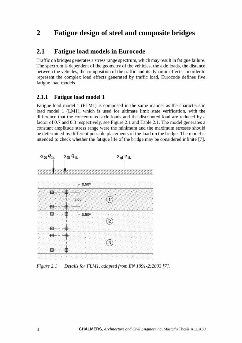
2.1.1 Fatigue load model 1
Fatigue load model 1 (FLM1) is composed in the same manner as the characteristic
load model 1 (LM1), which is used for ultimate limit state verification, with the
difference that the concentrated axle loads and the distributed load are reduced by a
factor of 0.7 and 0.3 respectively, see Figure 2.1 and Table 2.1. The model generates a
constant amplitude stress range were the minimum and the maximum stresses should
be determined by different possible placements of the load on the bridge. The model is
intended to check whether the fatigue life of the bridge may be considered infinite [7].
Figure 2.1 Details for FLM1, adapted from EN 1991-2:2003 [7].
CHALMERS Architecture and Civil Engineering, Master’s Thesis ACEX30 5
Table 2.1 Concentrated axle loads and distributed loads for FLM1, according to
EN 1991-2:2003 [7].
Lane Number 𝑸𝒊𝒌
[kN]
𝒒𝒊𝒌
[kN/m2]
1 210 2.7
2 140 0.75
3 70 0.75
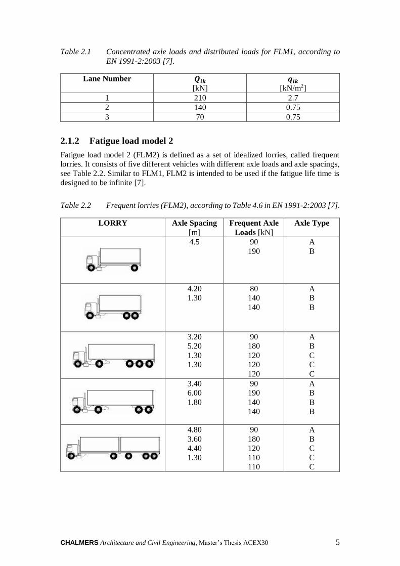
2.1.2 Fatigue load model 2
Fatigue load model 2 (FLM2) is defined as a set of idealized lorries, called frequent
lorries. It consists of five different vehicles with different axle loads and axle spacings,
see Table 2.2. Similar to FLM1, FLM2 is intended to be used if the fatigue life time is
designed to be infinite [7].
Table 2.2 Frequent lorries (FLM2), according to Table 4.6 in EN 1991-2:2003 [7].
LORRY Axle Spacing
[m]
Frequent Axle
Loads [kN]
Axle Type
4.5 90
190
A
B
4.20
1.30
80
140
140
A
B
B
3.20
5.20
1.30
1.30
90
180
120
120
120
A
B
C
C
C
3.40
6.00
1.80
90
190
140
140
A
B
B
B
4.80
3.60
4.40
1.30
90
180
120
110
110
A
B
C
C
C

CHALMERS, Architecture and Civil Engineering, Master’s Thesis ACEX30 6
2.1.3 Fatigue load model 3
Fatigue load model 3 (FLM3) consists of one vehicle with four axles, see Figure 2.2.
The force of each axle is 120 kN and each tire has a contact surface represented by a
square with a length of 0.40 m [7]. FLM3 is intendent to be used with the simplified λ-
method, see Section 2.2, where the calculated stress range should be less than or equal
to the fatigue strength of the investigated weld detail [8]
Figure 2.2 Geometry of fatigue load model 3, adapted from [7].
2.1.4 Fatigue load model 4
Fatigue load model 4 (FLM4) consists of a set of five standardized vehicles, which are
consistent with the most common heavy vehicles on European roadways [8]. In
addition, FLM4 includes three different traffic types where the proportion of the lorries
vary, representing local traffic, medium distance traffic and long-distance traffic, see
Table 2.3. Similar to FLM3, FLM4 is intended to be used for verification for finite
fatigue life [7].

CHALMERS Architecture and Civil Engineering, Master’s Thesis ACEX30 7
Table 2.3 Geometry and distribution of the lorries in FLM4, according to Table 4.7
in EN 1991-2:2003 [7].
VEHICLE TYPE TRAFFIC TYPE
Long
distance Medium
distance
Local
traffic
LORRY
Axle
Spacing
[m]
Equivalent
Axle Loads
[kN]
Lorry percentage Axle
Type
4.5 90
190
20.0 40.0 80.0 A
B
4.20
1.30
80
140
140
5.0 10.0 5.0 A
B
B
3.20
5.20
1.30
1.30
90
180
120
120
120
50.0 30.0 5.0 A
B
C
C
C
3.40
6.00
1.80
90
190
140
140
15.0 15.0 5.0 A
B
B
B
4.80
3.60
4.40
1.30
90
180
120
110
110
10.0 5.0 5.0 A
B
C
C
C
2.1.5 Fatigue load model 5
Fatigue load model 5 (FLM5) is based on measured traffic data. The data is
supplemented with statistical extrapolations to accommodate future traffic increases
[7]. FLM5 is intended to be used to verify the fatigue strength of complex bridges or
bridges with unusual traffic [8].
2.2 Fatigue verification methods
Eurocode defines two methods for fatigue verification in bridges.

CHALMERS, Architecture and Civil Engineering, Master’s Thesis ACEX30 8
2.2.1 The λ-coefficient method
The equivalent damage method, also known as the λ-coefficient method, is a simplified
method. The idea is that the fatigue damage caused by the actual stress range spectrum
from traffic can be described by one equivalent stress range which is obtained with a
damage equivalent factor [8]. The largest stress range generated by fatigue load model
3, ∆𝑆𝑝, is multiplied by a factor λ in order to represent the equivalent stress range from
real traffic 2∙106 stress cycles, see Equation (2.1).
∆SE,2 = λ ∙ ϕ2 ∙ ∆Sp (2.1)
Where;
𝜆 is the fatigue damage equivalent factor related to 2∙106 cycles;
Φ2 is the damage equivalent dynamic factor.
The fatigue damage equivalent factor, for road bridges, is obtained by Equation (2.2).
The λ-coefficients are presented in EN 1993-2 Section 9.5.2.
λ = λ1 ∙ λ2 ∙ λ3 ∙ λ4 ≤ λmax (2.2)
Where;
λ1 is the span factor, considering the length of the critical influence line;
λ2 is the factor considering the traffic volume;
λ3 is the factor considering the design life of the bridge;
λ4 is the factor considering traffic in additional lanes;
λmax is maximum λ-value considering the fatigue limit.
The equivalent stress range should be verified against the fatigue strength of the studied
detail category, according to Equation (2.3).
γFf ∙ ΔSE2 ≤ ∆Sc
γMf (2.3)
Where;
γFf is the partial safety factor for fatigue loading;
γMf is the partial factor for fatigue resistance.
2.2.2 Palmgren-Miner’s damage accumulation method
A stress range spectrum generated by traffic loads can be very complex, with varying
magnitude and frequency. A stress range spectrum such as in Figure 2.3 should be
transformed into one or more equivalent constant amplitudes that generate an
equivalent fatigue damage as the real loading situation. This can be done by first
transforming the variable amplitude load history into individual load cycles using cyclic
count methods such as the rainflow- or the reservoir counting method [1].

CHALMERS Architecture and Civil Engineering, Master’s Thesis ACEX30 9
Figure 2.3 To the left: Stress range spectrum with variable amplitude. To the right:
The resulting histogram using a cyclic counting method, adapted from
[1].
Performing the fatigue design can be done by applying the Palmgren-Miner damage
accumulation rule to the obtained stress ranges from the cycle counting. The method is
based on the assumption that the fatigue damage is cumulative and irreversible. In other
words, the fatigue life, represented by an S-N curve, for a certain detail is consumed
after N cycles of a certain stress range [1]. If the number of stress cycles n < N, the
accumulated damage can be calculated as:
𝐷 =𝑛
𝑁 (2.4)
With a spectrum as shown in Figure 2.3, with a number i loading blocks with a certain
stress range, Δ𝜎𝑖, and corresponding number of cycles, ni, the total accumulated fatigue
damage is obtained by the sum of the fatigue damage caused by each individual loading
block, see Equation (2.5).
𝐷 = ∑ 𝐷𝑖 = ∑𝑛𝑖
𝑁𝑖𝑖𝑖 (2.5)
Where Ni is the number of cycles that would cause damage for a certain stress range,
Δ𝜎𝑖, see Equation (2.6).
𝑁𝑖 = 5∙106 (
Δ𝜎𝐷𝛾𝑀𝑓
𝛾𝐹𝑓 . Δ𝜎𝑖)
𝑚
(2.6)
For a design curve with a constant slope, m, the same damage, D, is caused by the
equivalent stress range, Δ𝜎𝐸, after the same total number of cycles, i.e.
𝐷𝐸 =∑ 𝑛𝑖
𝑛𝑖=1
𝑁=
Δσ𝐸𝑚
5∙106∙Δσ𝐷
𝑚 ∙ ∑ 𝑛𝑖𝑛𝑖=1 (2.7)
Which also can be expressed in terms of equivalent stress:

CHALMERS, Architecture and Civil Engineering, Master’s Thesis ACEX30 10
Δ𝜎𝐸 = √∑ 𝑛𝑖
𝑛𝑖=1 ∙Δσ𝑖
𝑚
∑ 𝑛𝑖𝑛𝑖=1
𝑚 (2.8)
For a histogram composed of several stress blocks with different stress ranges, the
equivalent stress range can be expressed as:
Δ𝜎𝐸 = √∑ 𝑛𝑖Δσ
𝑖
𝑚𝑖+∑ 𝑛𝑗Δσ𝑗
𝑚𝑖(Δ𝜎𝑗
Δ𝜎𝐷)
𝑚𝑗−𝑚𝑖
∑ 𝑛𝑖+ ∑ 𝑛𝑗
𝑚𝑖
(2.9)
Where;
i is the index of stress ranges larger than Δ𝜎𝐷, j is the index of stress ranges smaller than Δ𝜎𝐷,
mi is the slope of the tri-linear S-N curve above the knee point,
mj is the slope of the tri-linear S-N curve below the knee point.

CHALMERS Architecture and Civil Engineering, Master’s Thesis ACEX30 11
3 Post Weld Treatment (PWT) methods
In order to enhance the fatigue life of a welded structure it is important to apply good
design practice. However, in situations where critical detailing cannot be avoided post
weld improvements techniques can be used [5].
3.1 Classification of PWT methods
Post weld treatment (PWT) techniques generally either modify the weld geometry or
alter the residual stress state to become more beneficial in terms of fatigue. The aim
with the modification of the weld geometry is to reduce local stress peaks by creating a
smoother transition between the weld and the base plate, and improve the surface
quality by eliminating weld defects such as undercuts [5].
3.1.1 Weld geometry improvement methods
Weld geometry improvement methods can further be divided into two sub-categories
as shown in Figure 3.1.
Figure 3.1 Classification of weld geometry improvement methods. Adopted from
[9].
3.1.1.1 Grinding methods
The aim of grinding is to reduce stress concentrations by creating a smoother transition
between the weld toe and the base metal and by removing weld defects and undercuts
at the weld toe. The largest improvements of the fatigue strength is obtained for high
strength steel [9]. Grinding improves the fatigue life with a factor of 1.3 compared with
the as-welded state [10].
3.1.1.2 Re-melting methods
These techniques result in a re-melted area at the weld toe region. This creates a
smoother transition between the weld toe and the base metal without undercuts and slag
inclusions [9]. Tungsten Inert Gas (TIG) dressing can improve the fatigue strength by
a factor of 1.3 [10]. Re-melting methods are suitable for automation. However, it is

CHALMERS, Architecture and Civil Engineering, Master’s Thesis ACEX30 12
difficult to ensure that the result of the re-melting has been accomplished appropriately
[9].
3.1.2 Residual stress methods
Residual stress methods can further be divided into three sub-categories, peening-,
overloading- and thermal methods, as shown in Figure 3.2.
Figure 3.2 Classification of residual stress methods. Adapted from [9].
3.1.2.1 Peening methods
Peening is a cold working technique which plastically deforms the welded region
through impacts. This replaces the tensile residual stresses from the welding process
with favorable compressive residual stresses. The magnitude of the compressive
stresses is of the order of the yield stress of the material. The fatigue strength
improvement becomes greater the higher the strength steel. In addition to the induced
compressive residual stresses, the transition and weld undercuts at the weld toe are
smoothened out [9]. Both hammer- and needle peening improves the fatigue strength
by a factor of 1.3 for fy < 355 MPa and a factor of 1.5 for fy ≥ 355 MPa [10].
3.1.2.2 Overloading methods
Overloading methods is classified as mechanical methods, just as peening. Prior to
fatigue loading, static overloading can introduce compressive residual stresses at the
weld toe by local yielding in the range of 50 % to 90 % of the yield stress [9].

CHALMERS Architecture and Civil Engineering, Master’s Thesis ACEX30 13
3.1.2.3 Thermal methods
The primary aim of thermal methods is to remove tensile residual stresses by
introducing heat to the welded region [9]. When using thermal stress relief, the material
is heated to a temperature between 550 ℃ to 650 ℃. After a specified amount of time,
the material is cooled down in a controlled manner in order to not create new tensile
residual stresses [11].
3.2 High Frequency Mechanical Impact (HFMI)
In 2010, Commission XIII of the IIW [5] introduced the term high frequency
mechanical impact (HFMI) as a generic term to describe several related peening
technologies developed by different equipment manufacturers. The devices operate
similar to the older hammer- and needle peening tools but in general, the impact
frequencies are higher. The IIW defines the HFMI technologies to have impact
frequencies greater than 90 Hz.
This thesis focuses on the HFMI treatment. All results in Chapter 4, 5, 6 & 7 are related
to this technique.
3.2.1 Description of the process
Similar to hammer and needle peening, the HFMI equipment accelerates single or
multiple indenters against the weld toe region. The indenters cause plastic deformation
in the material which results in a change in geometry as well as compressive residual
stresses in the impacted area. The higher impact frequency of the HFMI treatment leads
to a greater treatment quality compared with the older methods since smaller spacing
between the indentations are generated which gives a smoother surface [12].
3.2.2 Influence of loading
Since high tensile residual stresses already exists at the weld toe of as-welded (AW)
joints, the fatigue strength is considered to be independent of load conditions, such as
high mean stress or maximum loads. The tensile residual stresses, which are of the order
of the yield stress, makes the local mean stress insensitive to changes in the subjected
load. The maximum loads can even result in a beneficial effect of the AW joint. Due to
the high stress concentrations at the weld toe, the overload events in VA loading can
cause local yielding and relax the existing residual stresses [3].
On the other hand, one of the mechanisms that improves the fatigue life of HFMI-
treated joints is the induced compressive residual stresses. When the tensile mean stress
increase, the compressive residual stresses reduces which making the following load
cycles more damaging. Overloads in VA-loading, e.g. due to high dead load or
individual large stresses, may result in that the structure yield locally and release the
compressive residual stresses permanently [13].
CHALMERS, Architecture and Civil Engineering, Master’s Thesis ACEX30 14
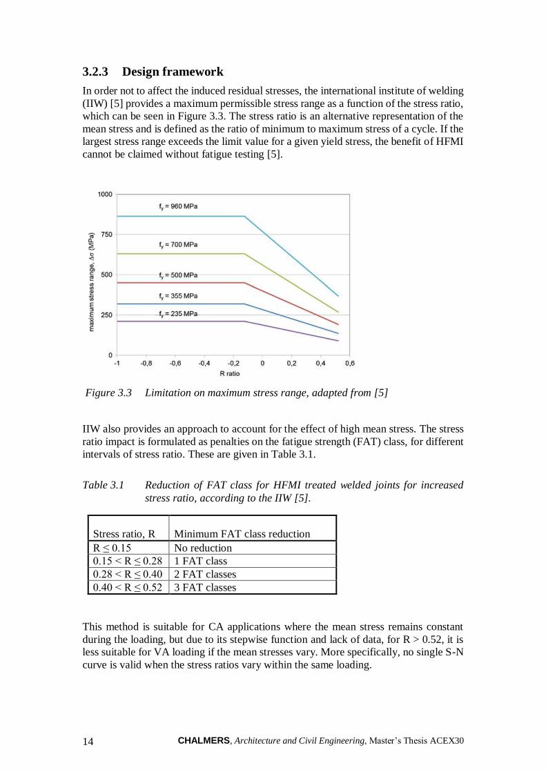
3.2.3 Design framework
In order not to affect the induced residual stresses, the international institute of welding
(IIW) [5] provides a maximum permissible stress range as a function of the stress ratio,
which can be seen in Figure 3.3. The stress ratio is an alternative representation of the
mean stress and is defined as the ratio of minimum to maximum stress of a cycle. If the
largest stress range exceeds the limit value for a given yield stress, the benefit of HFMI
cannot be claimed without fatigue testing [5].
Figure 3.3 Limitation on maximum stress range, adapted from [5]
IIW also provides an approach to account for the effect of high mean stress. The stress
ratio impact is formulated as penalties on the fatigue strength (FAT) class, for different
intervals of stress ratio. These are given in Table 3.1.
Table 3.1 Reduction of FAT class for HFMI treated welded joints for increased
stress ratio, according to the IIW [5].
Stress ratio, R Minimum FAT class reduction
R ≤ 0.15 No reduction
0.15 < R ≤ 0.28 1 FAT class
0.28 < R ≤ 0.40 2 FAT classes
0.40 < R ≤ 0.52 3 FAT classes
This method is suitable for CA applications where the mean stress remains constant
during the loading, but due to its stepwise function and lack of data, for R > 0.52, it is
less suitable for VA loading if the mean stresses vary. More specifically, no single S-N
curve is valid when the stress ratios vary within the same loading.

CHALMERS Architecture and Civil Engineering, Master’s Thesis ACEX30 15
Shams-Hakimi and Al-Emrani [3][6] suggested a modification of the IIW stress ratio
correction in order to make it suitable for VA applications in bridges, which were found
to include varying stress ratios for different cycles. Instead of reducing the fatigue
strength for every individual cycle, the strength was kept constant as the CA R=0.1
strength. The stress ranges were then magnified with a correction factor of
approximately 1.125 for every FAT class that would be reduced according to the IIW
method, see Figure 3.4. In addition, they also extrapolated the method to R=1.0 and a
polynomial fit was performed to generate a continuous expression, see Equation 3.1.
The continuous expression allows the Palmgren-Miner’s equivalent stress range,
Equation (3.2), to be modified to include the stress ratio effect, see Equation (3.3).
Figure 3.4 The IIW stepwise method together with Shams-Hakimi and Al-Emrani’s
[3][6] suggested mean stress correction, adapted from [6].
𝑓𝑖 = 0.5𝑅𝑖2 + 0.95𝑅𝑖 + 0.9 (3.1)
Δ𝑆𝑒𝑞 = √∑(𝑛𝑖∙Δ𝑆𝑖
𝑚)
∑ 𝑛𝑖
𝑚 (3.2)
Δ𝑆𝑒𝑞𝑅 = √∑(𝑛𝑖∙(Δ𝑆𝑖 ∙𝑓𝑖)𝑚)
∑ 𝑛𝑖
𝑚 (3.3)
3.2.3.1 Design framework for bridges
At present, there are no design methods for HFMI-treated joints included in the
Eurocodes. The most common fatigue verification of AW joints, in the Eurocodes is
the lambda method. As mentioned in the previous chapter, in Section 2.2.1, the lambda
method is carried out by calculating the stress range, ∆𝑆𝑝, generated by the fatigue load
model 3 (FLM3) [14]. To obtain the equivalent stress range from the real traffic, ∆𝑆𝑝
is multiplied with a set of 𝜆 factors that include the span length factor, the volume of
the traffic, the intended service life of the bridge and a factor for traffic in more than
one lane.
CHALMERS, Architecture and Civil Engineering, Master’s Thesis ACEX30 16
To cover HFMI-treated joints, Shams-Hakimi and Al-Emrani [3][6] suggests an
extension of the method, by adding a new factor 𝜆𝐻𝐹𝑀𝐼 . The factor needs to include the
stress ratio variation of the real traffic and the effect of self-weight as well as the
relationship of the fatigue strength to the mean stress or stress ratio. The suggested
𝜆𝐻𝐹𝑀𝐼 factor is the ratio of the modified equivalent stress range, ∆𝑆𝑒𝑞𝑅 , and the
equivalent stress range ∆𝑆𝑒𝑞 , see Equation (3.4).
𝜆𝐻𝐹𝑀𝐼 =∆𝑆𝑒𝑞𝑅
∆𝑆𝑒𝑞 (3.4)
The VA load is not known by the designer and thereby, neither is the modified
equivalent stress range, ∆𝑆𝑒𝑞𝑅 . To be able to predict 𝜆𝐻𝐹𝑀𝐼 , Shams-Hakimi and Al-
Emrani [3][6] used 55,000 measured Swedish vehicles to calculate the factor for
different spans, support conditions and self-weights. The results were simplified into
two different equations, one for span sections, Equation (3.5), and one for support
sections, Equation (3.6). 𝜆𝐻𝐹𝑀𝐼 varies with a factor 𝜙, which is the ratio of the stress
caused by the self-weight, 𝑆𝑆𝑊, and the largest stress range caused by the real traffic,
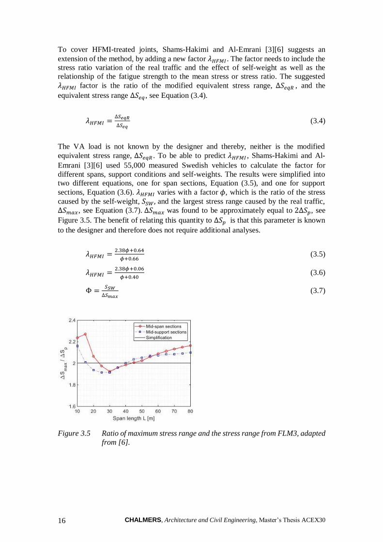
∆𝑆𝑚𝑎𝑥, see Equation (3.7). ∆𝑆𝑚𝑎𝑥 was found to be approximately equal to 2∆𝑆𝑝, see
Figure 3.5. The benefit of relating this quantity to ∆𝑆𝑝 is that this parameter is known
to the designer and therefore does not require additional analyses.
𝜆𝐻𝐹𝑀𝐼 =2.38𝜙+0.64
𝜙+0.66 (3.5)
𝜆𝐻𝐹𝑀𝐼 =2.38𝜙+0.06
𝜙+0.40 (3.6)
Φ =𝑆𝑆𝑊
∆𝑆𝑚𝑎𝑥 (3.7)
Figure 3.5 Ratio of maximum stress range and the stress range from FLM3, adapted
from [6].
CHALMERS Architecture and Civil Engineering, Master’s Thesis ACEX30 17
4 Validity of the traffic data
The 𝜆𝐻𝐹𝑀𝐼 -method, proposed by Shams-Hakimi and Al-Emrani [3][6], is limited to
Swedish road traffic. 55,000 Swedish vehicles were used as a representation for the real
traffic.
In this chapter, it is investigated whether the traffic data pool, used by Shams-Hakimi
and Al-Emrani [3][6], is large enough to represent Swedish road traffic. In addition, a
comparison with traffic data from the Netherlands was made in order to consider if the
Swedish traffic data is representative for other European countries.
4.1 Increased traffic data pool
To ensure that the traffic data of 55,000 vehicles is enough to represent Swedish road
traffic, the same methodology to derive 𝜆𝐻𝐹𝑀𝐼 was performed with a larger traffic pool.
4.1.1 The Swedish traffic data pool
The calculations are based on traffic measurements performed by The Swedish Road
Administration during the years 2005 to 2009. The sorted and processed traffic data has
been obtained from Prof. John Leander and previous work related to this data was
published by Leander [15]. The measurements are performed by the technique Bridge
Weight in Motion (BWIM), where a bridge together with strain gauges are used as a
scale to characterize the vehicles when they pass by. The traffic data contains 872,090
vehicles, measured at different locations distributed over the whole country.
4.1.2 Result
The vehicles were driven over a 10 meter simply supported bridge and a continuous
two span bridge with equal span lengths of 10 meter. Shams-Hakimi and Al-Emrani
[3][6] made simulations on various span lengths and conclude that the most
conservative result was obtained for the shortest spans. This is since a short span bridge
can generate additional secondary cycles while a longer bridge mainly generates one
cycle per vehicle. The additional cycles tend to have a higher minimum stress compared
with the main cycles and therefore contribute to a higher mean stress effect. As
mentioned in Chapter 3, the expression of 𝜆𝐻𝐹𝑀𝐼 was simplified to one equation for
span sections and one equation for mid-support sections. The locations that were found
to represent the two different sections were in 0.50L of a simply supported bridge and
0.85L of a symmetric double-span bridge. An S-N slope of 𝑚 = 5 was used to calculate
both the Palmgren-Miner’s equivalent stress range, ∆𝑆𝑒𝑞 , and the modified equivalent
stress range, ∆𝑆𝑒𝑞𝑅 , according to Equation (3.3) [3][6].
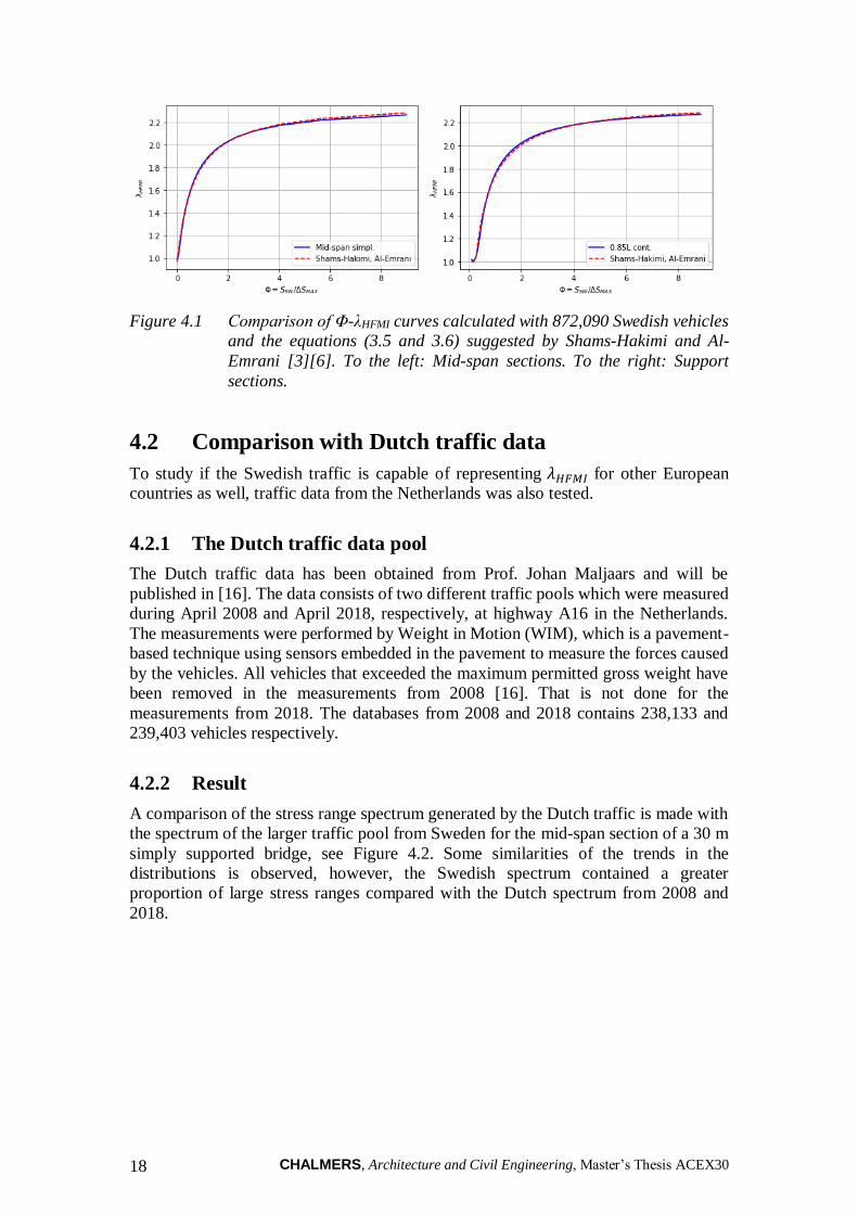
Figure 4.1 shows a comparison of the generated Φ-λHFMI curves for the larger Swedish
data pool with the expressions for 𝜆𝐻𝐹𝑀𝐼 according to equation (3.5) and (3.6). The
equations purposed by Shams-Hakimi and Al-Emrani [3][6] produce equal or
conservative 𝜆𝐻𝐹𝑀𝐼-values for all Φ except for Φ ≈ 2 in the support section, where the
real traffic of the larger Swedish data pool generated a maximum difference of 1.03 %.
CHALMERS, Architecture and Civil Engineering, Master’s Thesis ACEX30 18
Figure 4.1 Comparison of Φ-λHFMI curves calculated with 872,090 Swedish vehicles
and the equations (3.5 and 3.6) suggested by Shams-Hakimi and Al-
Emrani [3][6]. To the left: Mid-span sections. To the right: Support
sections.
4.2 Comparison with Dutch traffic data
To study if the Swedish traffic is capable of representing 𝜆𝐻𝐹𝑀𝐼 for other European
countries as well, traffic data from the Netherlands was also tested.
4.2.1 The Dutch traffic data pool
The Dutch traffic data has been obtained from Prof. Johan Maljaars and will be
published in [16]. The data consists of two different traffic pools which were measured
during April 2008 and April 2018, respectively, at highway A16 in the Netherlands.
The measurements were performed by Weight in Motion (WIM), which is a pavement-
based technique using sensors embedded in the pavement to measure the forces caused
by the vehicles. All vehicles that exceeded the maximum permitted gross weight have
been removed in the measurements from 2008 [16]. That is not done for the
measurements from 2018. The databases from 2008 and 2018 contains 238,133 and
239,403 vehicles respectively.
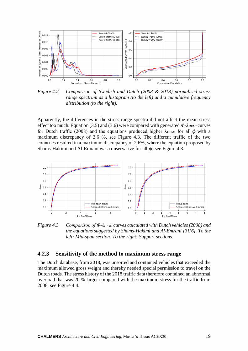
4.2.2 Result
A comparison of the stress range spectrum generated by the Dutch traffic is made with
the spectrum of the larger traffic pool from Sweden for the mid-span section of a 30 m
simply supported bridge, see Figure 4.2. Some similarities of the trends in the
distributions is observed, however, the Swedish spectrum contained a greater
proportion of large stress ranges compared with the Dutch spectrum from 2008 and
2018.
CHALMERS Architecture and Civil Engineering, Master’s Thesis ACEX30 19
Figure 4.2 Comparison of Swedish and Dutch (2008 & 2018) normalised stress
range spectrum as a histogram (to the left) and a cumulative frequency
distribution (to the right).
Apparently, the differences in the stress range spectra did not affect the mean stress
effect too much. Equation (3.5) and (3.6) were compared with generated Φ-λHFMI curves
for Dutch traffic (2008) and the equations produced higher λHFMI for all 𝜙 with a
maximum discrepancy of 2.6 %, see Figure 4.3. The different traffic of the two
countries resulted in a maximum discrepancy of 2.6%, where the equation proposed by
Shams-Hakimi and Al-Emrani was conservative for all 𝜙, see Figure 4.3.
Figure 4.3 Comparison of Φ-λHFMI curves calculated with Dutch vehicles (2008) and
the equations suggested by Shams-Hakimi and Al-Emrani [3][6]. To the
left: Mid-span section. To the right: Support sections.
4.2.3 Sensitivity of the method to maximum stress range
The Dutch database, from 2018, was unsorted and contained vehicles that exceeded the
maximum allowed gross weight and thereby needed special permission to travel on the
Dutch roads. The stress history of the 2018 traffic data therefore contained an abnormal
overload that was 20 % larger compared with the maximum stress for the traffic from
2008, see Figure 4.4.

CHALMERS, Architecture and Civil Engineering, Master’s Thesis ACEX30 20
Figure 4.4 Normalised stress history generated by the database from 2018 (to the
left) and by the database from 2008 (to the right).
Figure 4.5 reveals that the Dutch traffic from 2018 produces higher Φ-λHFMI curves
compared with equations (3.5) and (3.6) due to the abnormally large ∆𝑆𝑚𝑎𝑥 . This
reveals a sensitivity of this method of representing λHFMI and justifies a redefinition of
Φ in order to compare the different databases in a representative manner. Of course, a
better way of comparing the 2018 database to the proposed equations by Shams-Hakimi
and Al-Emrani [3][6] would be to exclude the extreme vehicles since this would make
a negligible difference in the actual mean stress effect. The simulation of the Dutch
traffic data from 2018 generated a maximum difference of 𝜆𝐻𝐹𝑀𝐼 that was 9 % higher
than predicted with Equation (3.5) and (3.6).
Figure 4.5 Comparison of Φ-λHFMI curves calculated with Dutch vehicles, measured
during April 2018, and the equation suggested by Shams-Hakimi and Al-
Emrani [3][6]. To the left: Mid-span section. To the right: Support
sections.

CHALMERS Architecture and Civil Engineering, Master’s Thesis ACEX30 21
5 Improvements of the Method
The results obtained in Chapter 4 have shown that the 55,000 vehicles that Shams-
Hakimi and Al-Emrani [3][6] used was enough to represent Swedish road traffic in a
satisfactory manner. It was also shown that the method was applicable to Dutch traffic
data from 2008 as well. On the other hand, the results showed that the method was
sensitive to abnormal overloads, therefore, a good comparison to the 2018 Dutch traffic
data could not be made.
In this chapter the same methodology will be performed, with the aim of altering the
method to become less sensitive to changes of the maximum stress range.
5.1 New definition of Φ
𝜆𝐻𝐹𝑀𝐼 depends on the factor 𝜙 which is the ratio of the stress caused by the self-weight
and the maximum stress range produced by the traffic, see Equation (3.7). To make the
method less sensitive to the stress range of a single vehicle, Φ needs to be redefined.
Palmgren-Miner’s equivalent stress range, ∆𝑆𝑒𝑞 , is a factor that represents all the
vehicles in the stress range spectrum and is therefore insensitive to the stress range
generated by a single vehicle. By redefining Φ as the ratio of the stress caused by the
self-weight and Palmgren-Miner’s equivalent stress range, see Equation (5.1), the
aforementioned sensitivity of 𝜆𝐻𝐹𝑀𝐼 to ∆𝑆𝑚𝑎𝑥 is eliminated.
Φ =𝑆𝑆𝑊
∆𝑆𝑒𝑞 (5.1)
In the followings, Φ-λHFMI curves are produced with the new definition of Φ for the
different traffic databases. The Swedish traffic generated the highest 𝜆𝐻𝐹𝑀𝐼 for all Φ
with a maximum difference of 1.9 % compared with the Dutch traffic from 2008, see
Figure 5.1.
Figure 5.1 Comparison of Φ-λHFMI curves calculated for real Swedish and Dutch
traffic (2008). To the left: Mid-span section. To the right: Support
sections.

CHALMERS, Architecture and Civil Engineering, Master’s Thesis ACEX30 22
It can also be noted that the abnormal overload, in the database from 2018, does not
affect the result in the same manner as before, see Figure 5.2. The Swedish traffic
produced the highest 𝜆𝐻𝐹𝑀𝐼 with the largest difference of 2.4 % which was found in the
support section.
Figure 5.2 Comparison of Φ-λHFMI curves calculated for real Swedish and Dutch
traffic (2018). To the left: Mid-span section. To the right: Support
sections.
5.1.1 Design framework
The Swedish traffic generated the highest 𝜆𝐻𝐹𝑀𝐼 in all cases. Therefore, it can be stated
that the expressions for 𝜆𝐻𝐹𝑀𝐼 in Equation (3.5) and (3.6) would also be valid for Dutch
traffic. However, in this section, new expressions are derived for 𝜆𝐻𝐹𝑀𝐼 for
compatibility with the new definition of Φ. The expressions should be based on the
results from the Swedish traffic data since it produced the highest 𝜆𝐻𝐹𝑀𝐼 . A curve fit of
the Φ-λHFMI curves, see Figure 5.3, resulted in one equation for mid-span sections, see
Equation (5.2), and one equation for mid-support sections, see Equation (5.3).
𝜆𝐻𝐹𝑀𝐼 =2.36𝜙+2.00
𝜙+2.15 (5.2)
𝜆𝐻𝐹𝑀𝐼 =2.36𝜙−0.42
𝜙+1.26 (5.3)
Figure 5.3 Φ-λHFMI curves proposed for use in the design of mid-span and mid-
support section.
CHALMERS Architecture and Civil Engineering, Master’s Thesis ACEX30 23
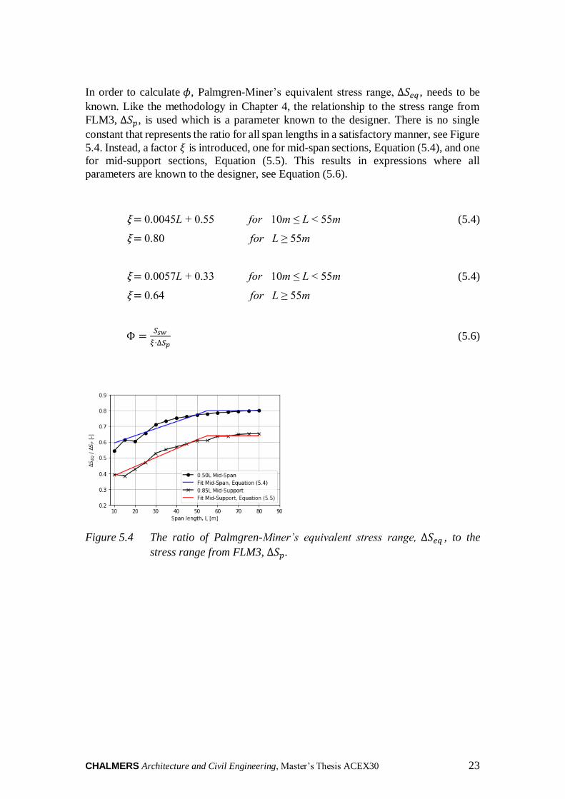
In order to calculate 𝜙, Palmgren-Miner’s equivalent stress range, ∆𝑆𝑒𝑞 , needs to be
known. Like the methodology in Chapter 4, the relationship to the stress range from
FLM3, ∆𝑆𝑝, is used which is a parameter known to the designer. There is no single
constant that represents the ratio for all span lengths in a satisfactory manner, see Figure
5.4. Instead, a factor 𝜉 is introduced, one for mid-span sections, Equation (5.4), and one
for mid-support sections, Equation (5.5). This results in expressions where all
parameters are known to the designer, see Equation (5.6).
ξ = 0.0045L + 0.55 for 10m ≤ L < 55m (5.4)
ξ = 0.80 for L ≥ 55m
ξ = 0.0057L + 0.33 for 10m ≤ L < 55m (5.4)
ξ = 0.64 for L ≥ 55m
Φ =𝑆𝑠𝑤
𝜉∙∆𝑆𝑝 (5.6)
Figure 5.4 The ratio of Palmgren-Miner’s equivalent stress range, ∆𝑆𝑒𝑞 , to the
stress range from FLM3, ∆𝑆𝑝.
CHALMERS, Architecture and Civil Engineering, Master’s Thesis ACEX30 24
6 Prediction of λHFMI using fatigue load models
The results obtained in Chapter 4 and Chapter 5 have confirmed that the mean stress
effect of HFMI-treated welds subjected to variable amplitude loading with varying
mean stress can be predicted using the method proposed by Shams-Hakimi and Al-
Emrani even for traffic from the Netherlands.
In this chapter, the Eurocode’s [17] fatigue load model 3 and 4 were studied in terms
of the mean stress effect. The aim was to investigate whether a fatigue load model can
be used to obtain the factor λHFMI directly, without using Equation (3.5) and Equation
(3.6).
For each load model, stress ranges were generated in the same manner as in Chapter 4
and 5 for span and support sections, however, in addition, a range of span lengths
between 10 and 80 meters were investigated instead of only 10 meters. In order to obtain
λHFMI, different approaches were needed for the two different load models.
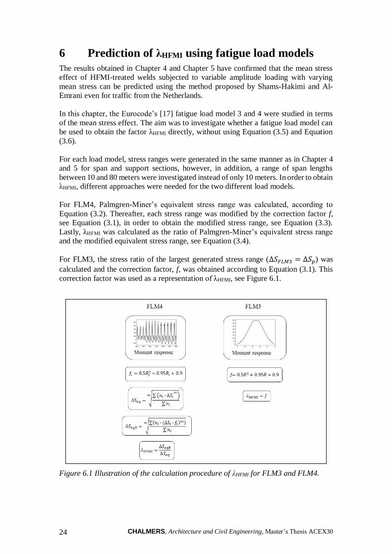
For FLM4, Palmgren-Miner’s equivalent stress range was calculated, according to
Equation (3.2). Thereafter, each stress range was modified by the correction factor f,
see Equation (3.1), in order to obtain the modified stress range, see Equation (3.3).
Lastly, λHFMI was calculated as the ratio of Palmgren-Miner’s equivalent stress range
and the modified equivalent stress range, see Equation (3.4).
For FLM3, the stress ratio of the largest generated stress range (∆𝑆𝐹𝐿𝑀3 = ∆𝑆𝑝) was
calculated and the correction factor, f, was obtained according to Equation (3.1). This
correction factor was used as a representation of λHFMI, see Figure 6.1.
Figure 6.1 Illustration of the calculation procedure of λHFMI for FLM3 and FLM4.
CHALMERS Architecture and Civil Engineering, Master’s Thesis ACEX30 25
6.1 Results
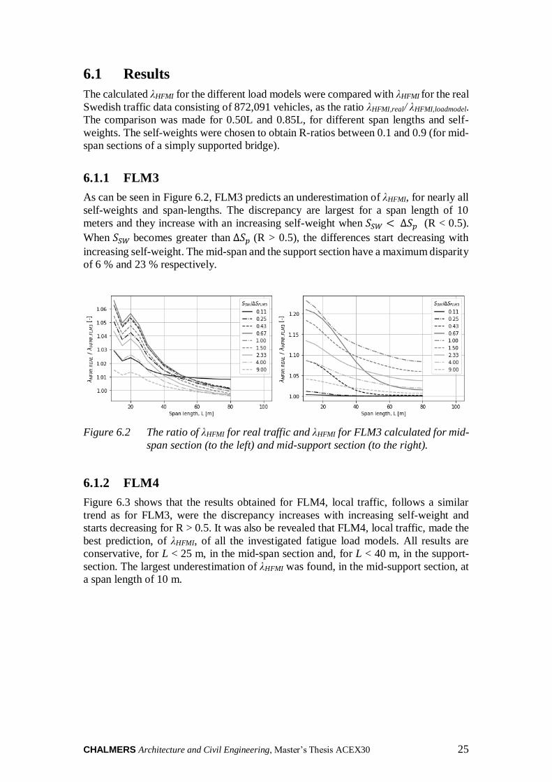
The calculated λHFMI for the different load models were compared with λHFMI for the real
Swedish traffic data consisting of 872,091 vehicles, as the ratio λHFMI,real/ λHFMI,loadmodel.
The comparison was made for 0.50L and 0.85L, for different span lengths and self-
weights. The self-weights were chosen to obtain R-ratios between 0.1 and 0.9 (for mid-
span sections of a simply supported bridge).
6.1.1 FLM3
As can be seen in Figure 6.2, FLM3 predicts an underestimation of λHFMI, for nearly all
self-weights and span-lengths. The discrepancy are largest for a span length of 10
meters and they increase with an increasing self-weight when 𝑆𝑆𝑊 < ∆𝑆𝑝 (R < 0.5).
When 𝑆𝑆𝑊 becomes greater than ∆𝑆𝑝 (R > 0.5), the differences start decreasing with
increasing self-weight. The mid-span and the support section have a maximum disparity
of 6 % and 23 % respectively.
Figure 6.2 The ratio of λHFMI for real traffic and λHFMI for FLM3 calculated for mid-
span section (to the left) and mid-support section (to the right).
6.1.2 FLM4
Figure 6.3 shows that the results obtained for FLM4, local traffic, follows a similar
trend as for FLM3, were the discrepancy increases with increasing self-weight and
starts decreasing for R > 0.5. It was also be revealed that FLM4, local traffic, made the
best prediction, of λHFMI, of all the investigated fatigue load models. All results are
conservative, for L < 25 m, in the mid-span section and, for L < 40 m, in the support-
section. The largest underestimation of λHFMI was found, in the mid-support section, at
a span length of 10 m.

CHALMERS, Architecture and Civil Engineering, Master’s Thesis ACEX30 26
Figure 6.3 The ratio of λHFMI for real traffic and λHFMI for FLM4 (local traffic)
calculated for mid-span section (to the left) and mid-support section (to
the right).
As can be seen in Figure 6.4 and Figure 6.5, FLM4 medium distance and long distance
obtained liberal results, for almost all cross-sections and span lengths. The largest
discrepancy was found to be 10 %, in the mid-support section, for short span bridges.
Figure 6.4 The ratio of λHFMI for real traffic and λHFMI for FLM4 (medium distance)
calculated for mid-span section (to the left) and mid-support section (to
the right).
Figure 6.5 The ratio of λHFMI for real traffic and λHFMI for FLM4 (long distance)
calculated for mid-span section (to the left) and mid-support section (to
the right).

CHALMERS Architecture and Civil Engineering, Master’s Thesis ACEX30 27
Figure 6.3 showed that FLM4, local traffic, obtained the best prediction of λHFMI.
Therefore, further studies were performed for this fatigue load model. The ratios of
λHFMI for real traffic and λHFMI for FLM4 (local traffic) were calculated for two types of
continuous bridges with unequal span lengths to investigate a wider variety of bridge
geometries. The first type was a three-span bridge with a middle span of L2 = 0.7L1, see
Figure 6.6, whereas the second type was a three-span bridge with a middle span of L2
= 1.3L1, as can be seen in Figure 6.9.
Figure 6.7 and Figure 6.8 shows the prediction of λHFMI was more liberal compared with
the results in Figure 6.3. The largest underestimation of λHFMI was found to be 10 %
and was obtained for short span bridges, in the mid-span section of the middle span.
Figure 6.6 Geometry and investigated locations of the asymmetric bridge, with a
shorter mid-span.
Figure 6.7 The ratio of λHFMI for real traffic and λHFMI for FLM4 (local traffic)
calculated for 0.50L1 (to the left) and 0.85L1 (to the right).
Figure 6.8 The ratio of λHFMI for real traffic and λHFMI for FLM4 (local traffic)
calculated for 0.50L2 (to the left) and 0.15L2 (to the right).

CHALMERS, Architecture and Civil Engineering, Master’s Thesis ACEX30 28
Figure 6.10 and Figure 6.11 shows that the bridge with a longer mid-span obtained
similar results as the symmetric two-span bridge, see Figure 6.3. The largest
underestimation was 6 % and was found at 0.15L2.
Figure 6.9 Geometry and investigated locations of the asymmetric bridge, with a
longer mid-span.
Figure 6.10 The ratio of λHFMI for real traffic and λHFMI for FLM4 (local traffic)
calculated for 0.50L1 (to the left) and 0.85L1 (to the right).
Figure 6.11 The ratio of λHFMI for real traffic and λHFMI for FLM4 (local traffic)
calculated for 0.50L2 (to the left) and 0.15L2 (to the right).

CHALMERS Architecture and Civil Engineering, Master’s Thesis ACEX30 29
7 λHFMI in case-study bridges
Previous chapters have studied the variation of λHFMI, in mid-span and mid-support
sections for fictitious bridges. In this chapter, all the earlier investigated methods will
be performed, in all cross-sections, on three different girder bridges that have been built
in Sweden.
All the bridges, see Figure 7.1, are composite steel and concrete bridges which gives
unfavorable conditions for HFMI-treated welds due to the high mean stresses from the
self-weight. The bridges are adopted from Dr. Shams-Hakimi’s Phd. thesis where more
detailed information on the bridges has been published [3].
Figure 7.1 Span lengths for investigated bridges.
The calculations were carried out by only considering the moment variation along the
bridges. The magnitude of λHFMI will, therefore, differ from the actual λHFMI-values,
calculated with the real stress of the studied detail. However, the purpose of this study
was to compare the relationship between all the earlier investigated methods and real
traffic, which will remain the same. Bending moment influence lines were generated
for all sections with a spacing of 1 meter. Variation in bending stiffness, due to cracking
of the concrete deck and variations in the girder sections, were taken into account. The
self-weight of the bridges was defined by the steel girders, concrete deck and paving to
obtain realistic self-weights. The parameters used for the calculations is provided in
Appendix A.
Bridge 1 is a 32 meter simply supported bridge. FLM4 and the design framework
proposed by Shams-Hakimi and Al-Emrani [3][6] predict conservative λHFMI values for
all cross-sections along the bottom flange of the bridge, see Figure 7.2. The modified
design framework, presented in Section 5.1.1, generates a λHFMI that is equal or
conservative to the real traffic. FLM3 predicts liberal λHFMI values along the whole
beam. The top flange of the girder is in compression and all methods results in λHFMI =
1.0, see Figure 7.3.

CHALMERS, Architecture and Civil Engineering, Master’s Thesis ACEX30 30
Figure 7.2 λHFMI calculated in the bottom flange of Bridge 1.
Figure 7.3 λHFMI calculated in the top flange of Bridge 1.
Bridge 2 is a symmetric two-span bridge with span lengths of 28.3 meters. All methods
predict conservative λHFMI values, for the bottom flange, except from fatigue load model
3, see Figure 7.4. The same results are obtained for the top flange, see Figure 7.5.
Figure 7.4 λHFMI calculated in the bottom flange of Bridge 2.

CHALMERS Architecture and Civil Engineering, Master’s Thesis ACEX30 31
Figure 7.5 λHFMI calculated in the top flange of Bridge 2.
Bridge 3 consists of three continuous spans with a total length of 39.2 meters. The
design framework proposed by Shams-Hakimi and Al-Emrani [3][6] and the modified
method, presented in Section 5.1.1, give conservative results in both the bottom and top
flanges, see Figure 7.6 and Figure 7.7. In contrast, FLM3 and FLM4 underestimate
λHFMI in all cross-sections of the bottom flange. The largest difference is obtained in the
middle-span where the fatigue load models obtain a constant value of λHFMI = 1.0.
Figure 7.6 λHFMI calculated in the bottom flange of Bridge 3.
Figure 7.8 λHFMI calculated in the top flange of Bridge 3.

CHALMERS, Architecture and Civil Engineering, Master’s Thesis ACEX30 32
8 Discussion
The discussion is divided in to four parts, one for each Chapter 4, 5, 6 and 7.
8.1 Chapter 4 – Validity of the data
The traffic data base used by Shams-Hakimi and Al-Emrani [3][6], containing 55,000
Swedish trucks was shown to be enough to represent the traffic on Swedish roads in
terms of the mean stress effect. The maximum discrepancy of 1.03 % compared with
the larger data base of Swedish traffic is considered unimportant in this context.
Chapter 4 also showed that the method is applicable on Dutch road traffic. The Swedish
traffic generated larger λHFMI for all Φ and is thereby conservative. This makes the
Swedish traffic suitable as the basis for derivation of expressions for λHFMI. The
similarities of the λHFMI-Φ curves for the two countries (Figure 4.3) can be explained
by studying the stress range spectra, in Figure 4.2. The two spectra are relatively close
to each other were the distribution of the stress ranges follow the same trends. However,
it can be seen that the Swedish database contains a greater proportion of larger stress
ranges compared with the Dutch traffic database. That could be explained by the fact
that Sweden is one of the countries in Europe that allows the highest maximum weight
of lorries [18] and this could be the reason why Swedish traffic produced a greater mean
stress effect (2.6% higher lambda at most). The maximum permitted gross weight on
Swedish and Dutch roads is 60 ton and 50 ton respectively.
Since the method is dependent on the maximum stress range, the comparison of
different traffic pools will vary depending on the stress range produced by a single
vehicle, which is not appropriate. The abnormal stress range in Figure 4.4 affected the
λHFMI-Φ curves too much to give representative comparisons.
8.2 Chapter 5 – Improvements of the method
By redefining Φ as the ratio of the stress caused by the self-weight and Palmgren-
Miner’s equivalent stress range, the λHFMI-Φ curves are no longer dependent of only
one vehicle and the problem of comparing different traffic pools can be overcome. The
results in Figure 5.2 show that the maximum stress range does not affect λHFMI in the
same manner. A comparison of Figure 5.1 and Figure 5.2 shows that the traffic data
from 2018 generated lower λHFMI than the traffic data from 2008. This can be explained
by the fact that the traffic data from 2018 had a lower equivalent stress range, even if it
contained a larger maximum stress range.
The Swedish traffic data base generated larger λHFMI compared with the Dutch traffic
data base, in both sections and for all Φ.
8.3 Chapter 6 – Prediction of λHFMI using fatigue load
models
It was investigated whether Eurocode’s fatigue load models 3 and 4 could be used as
an alternative to the approaches in the previous chapters to account for the mean stress
effect directly. An obvious benefit of this approach would be that no distinction

CHALMERS Architecture and Civil Engineering, Master’s Thesis ACEX30 33
between span and support section would be required which could hopefully result in
less conservative predictions of the mean stress effect.
FLM3 resulted in a maximum discrepancy of 6 % in mid-span sections compared with
real traffic, which may considered to be acceptable. On the other hand, FLM3 gave a
λHFMI that was up to 23 % smaller than λHFMI for real traffic. This gives a large
underestimation of λHFMI. The greatest discrepancy was obtained, in support sections,
for low self-weights. This is since a lower self-weight stress makes the R-ratio more
sensitive to changes in the applied load. However, when the self-weight stress is low,
the detailed geometry of the vehicles becomes more important, i.e. axle loads and axle
distance. FLM3 is represented by only one vehicle which is not enough to represent
real traffic in mid-support sections.
FLM4, which contains five different vehicles, represented the real traffic in a better
manner than FLM3. FLM4, local traffic, was the fatigue load model that resulted in the
best agreement with the real traffic. The maximum discrepancy was, for all three traffic
types, found in the mid-support section. In Figure 6.3, it can be seen that the largest
disparity was obtained for Ssw/ΔSFLM4 = 0.43. Why the discrepancy was smaller for
lower self-weight proportions can be explained by the R-ratio limit of 0.1. SSW < 0.43
caused the majority of the stress cycles to have an R-ratio < 0.1, resulting in a correction
factor f =1.0 for these cycles for both the fatigue load model as well as the real traffic.
FLM3 and FLM4 medium- and long-distance traffic underestimated λHFMI in all
sections and for almost every span length. That results in a prediction of the mean stress
effect that is unsafe. In contrast, FLM4 local traffic resulted in conservative predictions
of λHFMI for all span lengths of L > 20 m in mid-span sections and all L > 40m in mid-
support sections. Anyhow, there is a maximum underestimation of 4 %, found in the
mid-support section with a span length of 10 meter. The discrepancy is small could be
considered acceptable.
In order to cover a greater verity of bridge geometries, two different, asymmetric, three-
span bridges were investigated. It could be seen, in Figure 6.8, that the largest
underestimation of λHFMI increased to 10 %. The most considerable discrepancy was
found in the mid-span section of the middle support. Again, the smaller middle support
results in lower self-weight stress, compared with the earlier studied bridges, which
makes the R-ratio more sensitive for changes in the applied load.
Figure 7.1 shows a comparison of the normalized stress range spectrum of the larger
Swedish traffic pool, as a cumulative frequency distribution, compared with the
different traffic types of FLM4. It can be seen that the local traffic generates the stress
range spectrum with a distribution closest to the Swedish traffic. This is suspected to
be the reason why the local traffic is the traffic type that predicts λHFMI best.

CHALMERS, Architecture and Civil Engineering, Master’s Thesis ACEX30 34
Figure 7.1 Normalised stress range spectrum as a cumulative frequency
distribution.
8.4 Chapter 7 - λHFMI in case-study bridges
In Chapter 7, all methods presented in this thesis were used to predict λHFMI for three
different case-study bridges. The results were compared with the real λHFMI values
coming from the larger Swedish traffic pool/data base.
It could be seen that FLM3 obtained liberal λHFMI values, in all cross-sections, for all
bridges. However, it should be noticed that the predicted values were still close to the
real λHFMI values, in most of the cross-sections, for all bridges. FLM4, local traffic,
obtained an even closer prediction. The results from bridge 1 and 2, see Figure 7.2-7.5,
showed that FLM4 generates conservative or equal λHFMI values in all cross-sections.
On the other hand, for Bridge 3, were liberal results obtained. The prediction gave an
underestimation, in all cross-sections, along the bottom flange of the beam. The most
inadequate estimation was found in the second span where the estimated values
deviated from the trend of the real values. This corresponds well with the study of the
three-span bridge, with a smaller middle span, presented in Chapter 6 (Figure 6.6), were
the most considerable prediction was obtained in the mid-span section of the middle
span, see Figure 6.8.
The method suggested by Shams-Hakimi and Al-Emrani [3][6], presented in Section
3.2.3.1, and the modified method, from Section 5.1.1, gave a good estimation of λHFMI
for all the three case-study bridges. The results are conservative or equal to the real
λHFMI, in all sections along the bridges. The modified equation obtains values that are
closer to the real λHFMI. This is since the stress range from FLM3 is multiplied by the
factor 𝜉, which varies with the span length, see Figure 5.4. In contrast, the method, from
Section 3.2.3.1, is using a constant factor of 2.0, independently of the span-length, see
Figure 3.5. This results in a more considerable discrepancy when the ratio between
∆𝑆𝑚𝑎𝑥 and ∆𝑆𝑝 increases.

CHALMERS Architecture and Civil Engineering, Master’s Thesis ACEX30 35
9 Conclusions
This thesis aimed to study realistic load effects on HFMI-treated bridges and to
investigate different methods to predict the impact of the mean stresses on the
performance of HFMI-treated welds. 1) Studies were conducted on the validity of
Shams-Hakimi and Al-Emrani’s [6][3] method for prediction of the mean stress effect
of HFMI-treated joints in bridges and 2) the applicability of the method on Dutch traffic
data was investigated. Alternative design frameworks for HFMI-treated joints were
investigated, 3), one method based on a modification of the proposal by Shams-Hakimi
and Al-Emrani [6][3] and, 4), one method based on the direct use of Eurocode’s fatigue
load models. Based on these outcomes, 5), the validity of all the methods was studied
on case-study bridges. Based on work in this thesis, the following conclusions can be
drawn.
• It was shown that the traffic data pool, used by Shams-Hakimi and Al-Emrani
in order to predict the mean stress effect for HFMI-treated joints in bridges, is
representative for Swedish road traffic. An increase of the traffic data pool by
1500% did not affect the results.
• The method suggested by Shams-Hakimi and Al-Emrani is also applicable for
Dutch traffic. The results obtained from the Swedish traffic showed a small
conservativity to the Dutch results, which together with the fact that Sweden is
one of the countries that allows the highest maximum gross-weight, strengthen
the procedure of basing the method on Swedish traffic data.
• In this thesis, a modified version of the original design framework is proposed.
The modification resulted in less conservative and more accurate predictions of
the mean stress effect.
• An investigation of the Eurocode’s fatigue load model 3 and 4 showed that
FLM4 local traffic is the fatigue load model that gives the best prediction of the
mean stress effect of HFMI-treated joints in bridges.
• A verification of all the methods was performed on three case-study bridges.
Both the method proposed by Shams-Hakimi and Al-Emrani and the modified
version obtained conservative and reasonable results for all three bridges. It was
shown that the modified method predicts values closer to real traffic.
9.1 Suggestions for further research
For future work, the following subjects are suggested.
• Using the modified design framework on real in-service measurements from
bridges to investigate the validity of the method.
• Using the proposed design framework to develop expressions to consider the
mean stress effect in railway bridges.

CHALMERS, Architecture and Civil Engineering, Master’s Thesis ACEX30 36
10 References
[1] Al-Emrani, M., Åkeström, B. (2013): Steel Structures. Report 2013:10,
Department of Civil and Environmental Engineering, Chalmers University of
Technology, Gothenburg, Sweden, 2013.
[2] Dahlvik, M., Eriksson, J. (2014): Load Effect Modelling in Fatigue Design of
Composite Bridges. Master’s Thesis, Royal Institute of Technology (KTH),
Stockholm, Sweden, 2014.
[3] Shams-Hakimi, P. (2020): Fatigue improvement of steel bridges with high-
frequency mechanical impact treatment. Ph.D. Thesis, Chalmers University of
Technology, Gothenburg, Sweden, 2020.
[4] Mosiello, A., Kostakakis, K. (2013): The benefits of Post Weld Treatment for
cost efficient and sustainable bridge design. Master’s Thesis, Chalmers
University of Technology, Gothenburg, Sweden, 2013.
[5] Marquis, G. B., Barsoum, Z. (2016): IIW Recommendations for HFMI
Treatment - For Improving the Fatigue Strength of Welded Joints.
Singapore: Springer Singapore, 2016.
[6] Shams-Hakimi, P., Al-Emrani, M. (2020): High-cycle variable amplitude
experiments and a design framework for bridge welds treated by high-frequency
mechanical impact. Submitted to Engineering Structures, 2020.
[7] Eurocode 1, Actions on structures – Part 2: Traffic loads on bridges. European
Committee for Standardization, 2003.
[8] Al-Emrani, M., Aygül, M. (2014): Fatigue design of steel and composite
bridges. Report 2014:10, Chalmers University of Technology, Gothenburg,
Sweden, 2014.
[9] Kirkhope, K. J., Bell, R., Caron, L. and Basu, R. I. (1996): Weld Detail Fatigue
Life Improvement Techniques (No. SR-1379). MIL Systems Engineering,
Ottawa, Canada, SR-1379, 1996.
[10] Hobbacher, A. (2008): Recommendations for Fatigue Design of Welded joints
and Components. International Institute of Welding, doc. XIII-2151r4-07/XV-
1254r4-07, Paris, France, 2008.
[11] Lindqvist, S., Holmgren, J. (2007): Alternative Methods for Heat Stress Relief.
Master’s Thesis, Luleå University of Technology, Luleå, 2007.
[12] Marquis, G. B., Mikkola, E., Yildirim, H. C., Barsoum, Z. (2013): Fatigue
strength improvement of steel structures by high-frequency mechanical impact:
proposed fatigue assessment guidelines, Weld World, vol. 57, no. 6, pp. 803-
822, Nov. 2013.
[13] Mikkola, E., Dore, M., Khurshiad, M. (2013): Fatigue strength of HFMI treated
structures under high R-ratio and variable amplitude loading. Procedia
Engineering, vol. 66, pp. 161-170, 2013, doi: 10.1016/j.proeng.2013.12.071.
[14] Eurocode 3, Design of steel structures – Part 2: Steel bridges. European
Committee for Standardization, 2006.

CHALMERS Architecture and Civil Engineering, Master’s Thesis ACEX30 37
[15] Leander, J. (2017): Kalibrering av lambda-metoden för dimensionering av stål-
och samverkansbroar I Sverige – en förstudie. KTH Royal Institute of
Technology, Stockholm, 2017.
[16] Maljaars, J. (2019): Evaluation of traffic load models for fatigue verification of
European road bridges. Submitted for publication in ENG Struct, 2019.
[17] Eurocode 1, Actions on structures – Part 2: Traffic loads on bridges. European
Committee for Standardization, 2003.
[18] Sundquist, H. Laster och lasteffekter av trafik på broar – Litteraturstudie.
Technichal Report nr. 98:66, KTH Royal Institute of Technology, Stockholm.

CHALMERS, Architecture and Civil Engineering, Master’s Thesis ACEX30 38
Appendix A
Properties of the case-study bridges All values are adopted from Dr. Shams-Hakimi’s Phd. thesis [3].
Loads
Self-weight loads per I-beam.
Bridge Steel [kN/m] Concrete [kN/m] Pavement [kN/m]
1 3.7 22 6.15
2 4.4 43 10.1
3 2.8 26 8.9
Proportion of traffic load in the investigated beam.
Bridge LDF
1 0.833
2 1.140
3 1.106
Cross section constants
Bridge 1:
Moment of inertia (short-term)
Coordinate [m] 0-9 9-23 23-32
I [m4] 0.0427 0.0495 0.0427
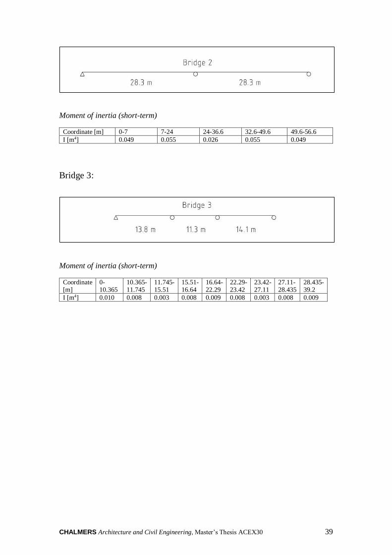
Bridge 2:
CHALMERS Architecture and Civil Engineering, Master’s Thesis ACEX30 39
Moment of inertia (short-term)
Coordinate [m] 0-7 7-24 24-36.6 32.6-49.6 49.6-56.6
I [m4] 0.049 0.055 0.026 0.055 0.049
Bridge 3:
Moment of inertia (short-term)
Coordinate [m]
0-10.365
10.365-11.745
11.745-15.51
15.51-16.64
16.64-22.29
22.29-23.42
23.42-27.11
27.11-28.435
28.435-39.2
I [m4] 0.010 0.008 0.003 0.008 0.009 0.008 0.003 0.008 0.009


DEPARTMENT OF ARCHITECHTURE AND CIVIL ENGINEERING
DIVISION OF STRUCTURAL ENGINEERING CHALMERS UNIVERSITY OF TECHNOLOGY
Gothenburg, Sweden
www.chalmers.se