the influence of economics and politics on the structure ... · the influence of economics and...
TRANSCRIPT
The influence of economics and politics on the structure of world trade and
investment flows
Shiro Armstrong and Peter Drysdale
Crawford School of Economics and Government
Australian National University
Abstract
The Asia Pacific region, and especially East Asia, has experienced rapid economic integration
without the ‘hard politics’ of legally binding economic and political treaties, unlike Europe
where integration has been institution-led. The ‘soft politics’ and market-led integration in
East Asia set against a background of political tensions and rivalries in key relationships in
the region. The paper measures trade and investment performance in the world economy.
This allows comparison of bilateral and regional trade and investment flows. A measure of
the effect of political distance on both trade and investment flows is also defined. The
growth of China-Japan trade and investment, despite political distance between the two
countries is discussed to highlight and elaborate on key findings. The analysis leads to five
conclusions. Multilateral institutions are important in reducing economic and political
distance between trading partners. While political relations do affect economic relations,
their effect is not important across the vast majority of trading relationships. The important
effects of political relations on economic relations come in today’s world via international
investment rather than through international trade. East Asian economies are leading trade
and economic integration, measured in terms of their trade and investment performance
and their impact on global trade and investment frontiers. Finally, of all the major regional
groupings, APEC and ASEAN stand out as arrangements in which there has been no trade
diversion, unlike the other formal regional groupings such as NAFTA and the EU in which
trade diversion is measurable. The paper finds an ‘APEC effect’, explains how economics can
dominate politics in international economic relations and recommends priority to
strengthening regional and international investment regimes to help ameliorate the likely
effects of politics on economic integration in the future.
Paper for presentation to 33rd Pacific Trade and Development Conference, The Politics and
the Economics of Integration in Asia and the Pacific, 6-8 October 2009, Taipei, Taiwan.

CONTENTS
Background ................................................................................................................................ 1
Measuring trade and investment performance ......................................................................... 2
Trade and FDI frontiers .............................................................................................................. 3
Trade performance ................................................................................................................ 3
FDI performance..................................................................................................................... 9
Explaining trade and investment performance ....................................................................... 14
The case of Japan and China .................................................................................................... 20
Conclusions ............................................................................................................................... 22
References ................................................................................................................................ 25
Data Annex ............................................................................................................................... 27

1
Background
The Asia Pacific region, and in particular the East Asia region, have seen rapid growth and
economic integration at an unprecedented speed and depth. The only other region with
comparably deep links is Europe. Asia is characterised by market-driven integration and
regionalisation, whereas in Europe integration was institution-led (Drysdale, 1988; ADB,
2008). In Europe economic integration followed political cooperation. This contrasts starkly
with East Asia where economic integration was the product of market forces, despite
political tensions and often absent the facilitation of formal diplomatic ties.
Market-led integration in Asia and the Pacific has been well documented with APEC coming
to play a significant role in trade and investment liberalisation and facilitation.
The regional rivalries and political competition have meant that the development, and the
robustness of, regional institutions have lagged and economic cooperation institutions have
been limited. Despite this, falling border barriers to trade and increasingly open investment
regimes have led to high trade shares and, in recent decades, the formation of production
networks and deep specialisation in regional production. The influence of political distance
on the structure and scale of bilateral and regional trade relationships and FDI over time is
of particular interest in the context of these developments.
This paper has two aims. First, it looks at the role of political distance, or the political
closeness between countries, on trade and investment worldwide and assesses whether
East Asian integration has been hampered by political distance among economies in the
region. The paper also compares the performance of trade and investment between
different regions. In doing so, special attention is played to the role of APEC. APEC is not a
trade or economic arrangement of the traditional kind among the economies in the Asia
Pacific region: thus far it has involved no preferential trade or other measures among its
members but has been ordered around the idea of ‘open regionalism’ and the principles of
non-discrimination in international economic dealings. APEC is built on the ‘soft politics’ of
regional economic cooperation not the ‘hard politics’ of legally binding economic and
political treaties. An important question is whether this mode of economic cooperation has
had any effect in boosting regional trade and economic integration and whether that effect
differs from the effect of other types of regional arrangement on international economic
integration. That is why measuring the impact that APEC has had on increasing trade and
investment in the region and also between the Asia Pacific region and the rest of the world
is of special interest in this analysis.
The next section sets out the concept of trade and investment frontiers as a means by which
to assess the influence of political and other factors on the realisation on trade potential.
Then the models and data that are used to assess trade and investment performance are
introduced, along with results of the analysis. After estimating performance, the following

2
section explains the performance around discussion of the important resistances to
international economic integration. The case of the Japan-China bilateral relationship is then
introduced to illustrate some of the findings and to show how political distance has been
overcome in East Asia. The conclusion draws out the five main findings and remarks on their
implications for policy.
Measuring trade and investment performance
In order to assess the performance of trade and FDI between regions, performance is
benchmarked by estimating trade and investment frontiers. Using a gravity model of trade
and a spatial FDI model, and applying stochastic frontier analysis, frontiers based on the
determinants of trade and FDI are estimated. Those frontiers are defined by the best trade
and FDI ‘technologies’ worldwide (Drysdale, Kalirajan and Huang, 2000; Armstrong, 2007;
Armstrong, 2009).
The performance of trade and FDI relationships can also be thought of as a measure of
economic distance where, since geographic distance is already controlled for, high
performance shows low resistance to goods or capital flows between countries. The most
liberal and free flowing trade and investment relationships are characterised by low
economic distance.
Both the trade frontier and the FDI frontier are estimated using the core variables of scale
(the GDPs of partner economies), distance, complementarity and multilateral resistances.
Unlike other gravity models of trade and FDI models, variables such as free trade
agreements (FTAs) or regional trade agreements (RTAs), measures of risk, tariff and other
non tariff barrier (NTB) variables, and language are not included in the model to estimate
the frontier and hence trade and investment performance, but are used to explain that
performance. The logic is that if a trade flow is high relative to its potential, as defined by
the frontier, its performance is high given the size of the trading countries, the distance they
are apart, the complementarities of their economic structures and controlling for the
influence of third countries. What explains the high levels of trade and investment
performance, then, may be similarity of language, membership of the same FTA or RTA, low
border barriers, and other factors.
To that list of possible explanatory variables of performance, the role of political distance is
added. Political distance is a measure of how ‘close’ two countries are politically, or
geopolitically, and how well they get along. Two countries which are political and security
allies can be described as being close in terms of political distance whereas two nations that
are political rivals, can be described as politically distant. Between these two extremes there
is a wide range of degrees of closeness and distance in the relationships between countries.
That will constrain or encourage interaction between their traders and investors. There is an
established literature that examines how politics affects trade (see Hirschman, 1945 and
3
Polacheck, 1980). A widening of political distance can increase uncertainty and lower
economic exchange between a pair of countries.
There is ample evidence of the link between the political relationships and trade (Mansfield
and Pollins, 2001; Mansfield and Pollins, 2003) and recognition that the direction of
causality and the lag times of the effect of political events on economic relations depend on
the character of the bilateral relationship. There is no comparable literature for FDI, but it
can be presumed that causality will run both ways and there will be lag length issues that
depend on the particular investment partners in analysing the effect of political factors on
investment flows in the same way as there is in analysing trade flows. Country pairs will not
necessarily hold a linear relationship over time in any analysis on FDI or trade.
In analysing resistances to FDI, the literature has included measures of host country
domestic political risk in studies, such as in done in Baltagi et al. (2007). The multinational
enterprise (MNE) international business literature focuses on differences between countries
and the implications for the modes of entry into markets by MNEs. Resistances have a
significant impact on the scale and structure of FDI (Ghemawat, 2007).
Trust and measures of cultural similarity, determined by religion, history of conflict and
ethnic similarities, are all factors that have been identified as having an effect on economic
linkages, including FDI (Guiso et al., 2004; Ghemawat, 2007). These resistances have also
been termed cultural distance in the FDI literature and used to describe the uncertainty that
a firm faces in investing in another country (Erramilli and D’Souza, 1995).
Fewer resources are likely to be committed in a trading relationship than are involved in
directly setting up a plant in a foreign country, such as is involved in an investment
relationship. Trade is therefore hypothesised to be less sensitive to increases in political
uncertainty than investment. In general it would be reasonable to assume FDI is more
affected by political developments than trade which is conducted more at arms-length. A
widening of political distance between two countries would be expected to affect FDI more
than trade.
Trade and FDI frontiers
Trade performance
The trade frontier is estimated using the following model.
(1) ijtijtijtijijjtitijt uvCOMPBorderrDistyyx 543210 lnlnlnlnln
Table 1 includes detail about these variables and the sources of data for their measurement.

4
Table 1 Variable description and data sources
Variable Description Data source Notes
xijt trade from i to j at time t
IMF’s Direction of Trade
Statistics (various years) and
gaps in the data are filled in
from the International Economic
Databank (IEDB)
Calculated from imports
instead of exports for
accuracy*.
yit Country i’s size (GDP) at
time t
World Development Indicators
(WDI) and at current prices
rDistij Relative distance from i to
j
Great circle distance between
capital cities of each country
was collected from the Chemical
Ecology of Insects website:
http://www.chemical-
ecology.net/
ik
jk
jk
ik
ij
ij
DistDist
DistrDist
Borderij Variable that takes on the
value of one if i and j
share a common land
border, zero otherwise.
COMPijt Complementarity index of
i’s trade with j at time t.
International Economic
Databank (IEDB), Australian
National University
k j
k
j
k
i
k
w
iw
i
k
i
ijM
M
MM
MM
X
XC
[see below]
Notes: * Importers have less incentive to under-report and imports are a more accurate reflection of trade flow values than reported
exports. The exception is European trade where there is tax incentive to under report imports due to the value added tax structure but import flows were used for consistency. This is common practice.
The complementarity index used here is from Drysdale (1967) and Drysdale and Garnaut
(1982):
k j
k
j
k
i
k
w
iw
i
k
i
ijM
M
MM
MM
X
XC
where X is exports, M is imports, subscripts denote country (i, j and world) and superscript k
implies commodity k. The index is calculated at the three digit level from the Australian
National University’s International Economic Databank1 for all combinations of countries
and years. The index captures the complementarity of trade structures between countries
and the higher the index implies a higher degree of complementarity.
vijt is an independently and identically distributed normal variable with mean zero and
variance σv2 and uijt is an independent and identically distributed non-negative variable
which usually has a half normal, truncated normal or exponential distribution (Kumbhakar
and Lovell, 2000).
The disturbance term vijt accounts for random variation in trade similar to the disturbance
term in the standard OLS model. The non-negative (or one sided) disturbance term, uijt,
1 http://iedb.anu.edu.au/

5
measures the difference between potential trade and actual trade. More precisely, it is the
amount of trade that falls short of the frontier for trade from country i to j at time t.2
The trade model is estimated for an unbalanced panel between 1980 and 2006. The data
includes a representative sample of world trade with the bilateral trade flows of 65
countries by 65 countries. The countries are listed in the Appendix. Some bilateral flows are
missing for some years due to data availability but given the large numbers of observations,
the data represent a relatively complete and balanced panel.
Table 1 shows results for ordinary least squares estimation in column (1). Column (2) is the
model estimated over the time-invariant country pair dimension and Column (3) is the same
model as Column (2) with additional time dummy variables which are not presented in the
results (to save space).
All coefficients are statistically significant at the 1 per cent level and the signs are as would
be expected. The larger two countries are, the more they trade and the further they are
apart, the less they trade. A complementary trade structure with a partner helps explain an
increase in trade as does sharing a border. The OLS coefficients on the GDP variables are
unity which is a result consistent with the gravity model literature.
2 For a detailed technical description of the estimation procedure see Coelli (1996) and Kumbhakar and Lovell (2000).

6
Table 2 OLS and MLE stochastic frontier estimation results
(1) (2) (3)
OLS
Frontier country
pair
Frontier w country pair & time dummies
Constant -33.37*** -18.49*** -20.39*** (0.2303) (0.1423) (0.1552)
lnGDPit 0.99*** 0.70*** 0.74*** (0.0066) (0.0041) (0.0049)
lnGDPjt 1.00*** 0.78*** 0.80*** (0.0061) (0.0038) (0.0039)
rDistij -3.59*** -2.28*** -2.28*** (0.0486) (0.0278) (0.0444)
Compijt 2.48*** 2.10*** 2.06***
(0.0265) (0.0210) (0.0331)
Borderij 0.92*** 0.98*** 0.98*** (0.0669) (0.0403) (0.0373)
sigma-squared 11.04 52.04*** 49.01*** (0.298) (0.3795)
Gamma 0.976*** 0.98***
Mu -14.26 -13.85
log likelihood function -244612 -212727
-211240
Number of observations 93382 93382
93382
Standard errors in parentheses;
* p < 0.05,
** p < 0.01,
*** p < 0.001
Table 3 presents trade performance results, or actual trade as a ratio of potential trade.
High trade performance (a high ratio of actual to potential trade) is associated with low
trade resistances. Conversely, low trade performance reveals high resistances to trade.

7
Table 3 Trade performance results, selected countries and years
Exporter Importer 1980 1985 1990 1995 2000 2006
EU EU 0.41 0.45 0.38 0.35 0.38 0.31
EU World 0.38 0.39 0.31 0.30 0.30 0.27
World EU 0.41 0.40 0.33 0.29 0.30 0.26
ASEAN ASEAN 0.49 0.36 0.49 0.50 0.49 0.51
ASEAN World 0.41 0.34 0.32 0.34 0.39 0.38
World ASEAN 0.38 0.35 0.36 0.36 0.35 0.32
APEC APEC 0.48 0.45 0.42 0.41
APEC World 0.32 0.31 0.33 0.32
World APEC 0.33 0.30 0.28 0.27
NAFTA NAFTA 0.39 0.41 0.37
NAFTA World 0.30 0.28 0.26
World NAFTA 0.30 0.32 0.33
South Asia South Asia 0.22 0.12 0.11 0.15 0.09 0.12
South Asia World 0.26 0.23 0.22 0.22 0.23 0.21
World South Asia 0.37 0.33 0.30 0.25 0.23 0.25
World World 0.37 0.34 0.30 0.28 0.30 0.28
other
China USA 0.29 0.42 0.48 0.53 0.55 0.58
China World 0.32 0.30 0.32 0.34 0.38 0.45
USA China 0.33 0.39 0.39 0.42 0.39 0.40
World China 0.27 0.36 0.27 0.28 0.28 0.32
Japan World 0.44 0.44 0.37 0.32 0.34 0.34
World Japan 0.41 0.35 0.26 0.22 0.23 0.23
China Taiwan 0 0 0 0.05 0.22 0.45
Taiwan China 0 0 0.01 0.45 0.47 0.55
China Japan 0.43 0.46 0.34 0.34 0.40 0.44
Japan China 0.36 0.36 0.30 0.37 0.38 0.42
Singapore Hong Kong 0.72 0.71 0.67 0.68 0.64 0.65
Singapore USA 0.63 0.64 0.64 0.61 0.62 0.58
United States Singapore 0.73 0.69 0.68 0.67 0.65 0.63
United States Hong Kong 0.64 0.61 0.62 0.62 0.58 0.55
United States World 0.45 0.37 0.36 0.36 0.34 0.30 World USA 0.41 0.39 0.35 0.33 0.35 0.34
Open economies that are close to large markets, such as are Singapore and Hong Kong,
perform better as expected and it is their trade characteristics, or trade technologies, that
define the frontier. The world average trade performance is declining over time. Given the
reductions in transportation and communications costs and the reduction of barriers to

8
trade, both at the border and beyond the border, reflected in rapidly increasing world trade
values, one might expect mean trade performance (realisation of potential) to be increasing.
The nature of stochastic frontier analysis means that the more variation there is in trade
performance, given the core determinants of trade, the lower the average performance is
likely to be. The best performers push the elasticities higher and the frontier shifts outwards
(an improvement in ‘trade technology’) meaning the average trade relationship has to keep
up with the best performers for average to grow. This observation is consistent with the
findings of Dowrick and DeLong (2003) who show that in the second half of the 20th century
there has been divergence in growth between those countries that have been at the global
table and those that have not, and that there has been convergence among those
economies that have opened their economies.
The increased variation in the sample over time and the outlier bilateral trade flows that
push the frontier outward means that most countries see performance fall over time as the
increased trade does not keep up with the frontier. There are, however, countries with
average performance increasing over time. For average export performance, China, Costa
Rica, India, Indonesia, Malaysia, Malta, Thailand and Vietnam all show a positive trend. For
imports, Chile, Ghana, Hong Kong, Hungary, Malaysia, Mexico, Turkey and Vietnam show a
positive trend. Half of these are found in East Asia with no other regional clustering.
Intra-ASEAN trade is consistently at around 50 per cent of potential trade, and appears to be
the most trade integrated region, consistent with findings by Armstrong, Drysdale and
Kalirajan (2008). ASEAN’s trade with the rest of the world (both imports at around 35 per
cent and exports at around 37 per cent) realise more of their trade potential with the rest of
the world than any other region. APEC and ASEAN members show less resistance to trade
than EU, North American and especially South Asian countries, both in their inter-regional as
well as their intra-regional trade.
A case of interest in this setting is China-Taiwan trade. Taiwan’s exports to China perform
remarkably well throughout the entire period under study, despite the absence of
diplomatic and direct trade links but China’s exports to Taiwan were severely repressed until
both economies’ accession to the WTO (Table 3). Taiwan’s imports from China still under-
perform compared with Taiwan’s exports to China. This is importantly because of the
Taiwanese embargoes that remain on imports from the mainland for political reasons, even
after accession to the WTO.
East Asian trade, it emerges, has been at the forefront of gains increased trade efficiency
through better utilisation of trade potential and, by implication, pushing out the global trade
frontier.
9
FDI performance
FDI models commonly use gravity model variables to explain FDI since both trade and FDI
have similar determinants. The latest models have succeeded in explaining FDI better by
recognising that FDI decisions are made differently from decisions to trade. Some MNEs use
FDI to avoid trade barriers and sell to the market in the host nation (horizontal FDI) while
others take advantage of cheaper factor prices to produce in a host nation and then export
that good (vertical FDI). There is also a more complex form of FDI where a source country
manages the knowledge-intensive input in production and uses a number of FDI
destinations in which there are different relative factor prices to produce parts and
components which are then traded to a third country (knowledge capital or complex vertical
FDI). Conventional gravity models cannot capture these different forms of FDI.
A MNE’s decision to invest in one country is dependent on the endowments in its country of
origin, factors in the potential host country and also neighbouring countries that could act
as both a substitute or complement for FDI. Multilateral resistances, in models such as that
of Baltaig et al. (2007), are captured differently in investment models from the case of trade
gravity models and include inverse distance weighted averages of all third country effects
for all determinants. Baltagi et al. and other FDI models of MNE behaviour3 have shown the
importance of including scale, distance, relative factor endowments and multilateral effects
in explaining FDI. Those determinants are chosen from models derived from firm level
behaviour and confirmed through empirical results that out-perform studies using only
gravity model variables.
Many studies model a two factor world, some with skilled and unskilled labour (see for
example Davis (2008)) and others with capital and labour. Results in studies such as Egger
and Pfaffermayer (2004), Baltagi et al. (2007) and Dee (2007) show that a three factor world
with skilled labour (or human capital), unskilled labour and physical capital, gives a better
explanation of FDI flows. This study builds on the models of Baltagi et al. (2007) and Dee
(2007). The model used here to estimate an investment frontier differs from Baltagi et al. in
two important ways. First, Baltagi et al. do not include a measure of distance as they
implicitly control for distance in the spatially correlated error term. They do this by using the
Gauss-Markov estimator to control for spatially correlated error terms. Spatially correlated
error terms capture the fact that a shock to one country affects other countries, and affects
countries which are closest the most.
This study follows Dee (2007) in its treatment of potentially spatially correlated error terms
deterministically with the inclusion of an FTA variable and a weighted FTA variable. The FTA
variable would usually be included in the second stage of explaining the performance results
but is used in the first stage where performance is estimated in order to control for spatially
correlated error terms. Relative distance and the FTA variables are used in this study to
3 See Blonigen (2005) for a review.

10
estimate the frontier and deterministically account for spatially correlated error terms. The
different nature of trade and FDI, with different modes of FDI entry into a country or
market, has meant different modelling derivations and therefore different approaches to
controlling for multilateral resistances.
Following both Dee and Baltagi et al., the model can account for different modes of FDI as
well as FDI determined by different factors. The difference from Dee’s model here is that it
does not include a risk variable and that a non-negative disturbance term is included that
makes it a stochastic frontier model.
2) Ft = β0 + β1dist + β2Gt + β3St + β4kt + β5ht + β6lt + β7Γt + β8Θt + β9FTAt
+ β10WGt + β11WSt + β12Wkt + β13Wht + β14Wlt + β15WΓt + β16WΘt
+ β17WRt + β18WFTAt + vt + ut
Where
Ft is the log of FDI (for FDI stock – FDI flows are also tested)
dist is the log of the great circle distance between capital cities of d and i.
Gt is the log of the sum of country d and country i GDPs: ln(GDPd + GDPi)
St is a measure of GDP similarity: (1 – sd2 – si
2)
where sd = GDPd /(GDPd + GDPi) and si = GDPi /(GDPd + GDPi)
kt is the log of the ratio of source country to destination country capital stock: ln(Kd/Ki)
ht is the log of the ratio of source country to destination country human capital: ln(Hd/Hi)
lt is the log of the ratio of source country to destination country unskilled labour: ln(Ld/Li)
Γt is an interaction term between Gt and kt: Gt kt
Θt is an interaction term between distance and the difference in capital and labour ratios:
dis(kt – lt)
FTAt is a variable that takes the value of one if country d and i have a free trade agreement
in force in year t.
W is a measure of multilateral effects interacted with each term. WGt, for example, is the
inverse distance weighted average of Gt between the source country and all third country
markets.

11
vt is an independently and identically distributed normal residual term that captures the
usual model disturbance from measurement error and other shocks that are no associated
with resistances to FDI.
ut is an independently and identically distributed non-negative variable that captures the
resistances to FDI.
FDI source countries in this analysis are the United States, Japan, Canada, Germany, France,
the United Kingdom and the Netherlands comprising seven of the largest eight FDI sources
globally4. The share of world FDI covered by this set of countries ranges from half to 70 per
cent depending on the year5. These source countries were chosen to minimise the missing
data problems and to make the panel as balanced as possible. There are ninety recipient
countries and they are listed in the Appendix. FDI stocks are used as is common practice and
FDI data are drawn from the OECD which has FDI data reported by OECD countries to OECD
and non-OECD member countries. The panel is highly unbalanced from 1982 to 2006.
Dummy variables for time are included and results for OLS and the frontier using maximum
likelihood estimation are presented.
GDP at purchasing power parity is used and is from the World Development Indicators along
with labour force and gross fixed capital formation data. Capital stock is calculated from the
perpetual inventory method from Leamer (1984) and explained in the Appendix. The human
capital data, from the International Labour Organisation and various national statistical
agencies, is the absolute number of graduates from tertiary institutions, such as universities,
in that country. The sum of the unskilled labour population and the population with a
tertiary qualification is equal to the total labour force.
Both trade and FDI frontier models can be estimated using any one of the following
programs: GAUSS, STATA, LIMDEP, and FRONTIER 4.1.
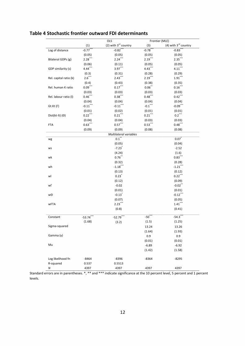
Most variables are statistically significant at a high degree of significance in explaining the
stock of FDI. All bilateral variables are statistically significant. The similar Baltagi et al. (2007)
specification and even closer specification of Dee (2007) did not have as many variables with
statistical significance as do the results in Table 4. As was the case in Baltagi et al. (2007) the
multilateral variables (those weighted by inverse distance) are jointly significant, confirming
their importance in explaining FDI. A simple F test on the multilateral variables in the OLS
model confirms joint statistical significance and a likelihood ratio test comes to the same
conclusion. The signs and the magnitudes of the coefficient estimates are all expected from
previous studies such as Dee (2007).
4 Switzerland ranks higher than the Netherlands but is not used as the coverage of recipient countries was not as
wide ranging as Dutch FDI. 5 Source: OECD Stata and UNCTAD FDI data.
12
Table 4 Stochastic frontier outward FDI determinants
OLS Frontier (MLE)
(1) (2) with 3rd country (3) (4) with 3rd country
Log of distance -0.77*** -0.82*** -0.78*** -0.83***
(0.05) (0.05) (0.05) (0.05)
Bilateral GDPs (g) 2.28*** 2.24*** 2.19*** 2.35***
(0.06) (0.11) (0.05) (0.05)
GDP similarity (s) 4.44*** 3.97*** 4.43*** 4.11***
(0.3) (0.31) (0.28) (0.29)
Rel. capital ratio (k) 2.6*** 2.43*** 2.19*** 1.91***
(0.4) (0.43) (0.38) (0.35)
Rel. human K ratio
(h)
0.09*** 0.17*** 0.06** 0.16***
(0.03) (0.03) (0.03) (0.03)
Rel. labour ratio (l) 0.46*** 0.38*** 0.48*** 0.42***
(0.04) (0.04) (0.04) (0.04)
Gt.Kt (Γ) -0.11*** -0.11*** -0.1*** -0.09***
(0.01) (0.02) (0.01) (0.01)
Dist(kt-lt) (Θ)
0.22*** 0.21*** 0.21*** 0.2***
(0.04) (0.04) (0.03) (0.03)
FTA 0.63*** 0.57*** 0.53*** 0.48***
(0.09) (0.09) (0.08) (0.08)
Multilateral variables
wg 0.1** 0.07*
(0.05) (0.04)
ws -7.23* -2.52
(4.24) (1.6)
wk 0.76** 0.83***
(0.32) (0.28)
wh -1.18*** -1.21***
(0.13) (0.12)
wl 0.23* 0.22***
(0.12) (0.09)
wΓ -0.02 -0.02**
(0.01) (0.01)
wΘ -0.13* -0.12***
(0.07) (0.05)
wFTA 2.23*** 1.41***
(0.8) (0.41)
Constant
-53.74*** -52.79*** -50*** -54.3***
(1.68) (3.2) (1.5) (1.25)
Sigma-squared 13.24 13.26
(1.64) (1.93)
Gamma (γ) 0.9 0.9
(0.01) (0.01)
Mu -6.89 -6.92
(1.42) (1.58)
Log likelihood fn
-8464
-8396
-8364
-8295
R-squared 0.537
0.5513
N 4397 4397 4397 4397
Standard errors are in parentheses. *, ** and *** indicate significance at the 10 percent level, 5 percent and 1 percent
levels.

13
Table 5 FDI performance results, 1982-2006
1982-
86
1987-
91
1992-
96
1997-
01
2002-
06
FDI source country
Canada 0.36 0.37 0.36 0.37 0.41
France 0.36 0.36 0.40 0.43
Germany 0.40 0.44 0.45 0.44 0.45
Japan 0.44 0.52 0.44 0.43 0.46
Netherlands 0.61 0.55 0.39 0.47 0.47
UK 0.42 0.47 0.38 0.47 0.46
USA 0.24 0.36 0.40 0.42 0.41
Selected FDI destinations
Australia 0.59 0.61 0.62 0.60 0.62
Brazil 0.48 0.50 0.53 0.52 0.52
China 0.13 0.26 0.29 0.34 0.32
France 0.22 0.38 0.38 0.28 0.48
Hong Kong 0.57 0.61 0.63 0.57 0.56
Mexico 0.30 0.35 0.39 0.39 0.39
Russia 0.03 0.27 0.41 0.45
Singapore 0.68 0.66 0.63
South Korea 0.43 0.40 0.32 0.34 0.40
Taiwan 0.38 0.40 0.40 0.40 0.46
Thailand 0.52 0.53 0.54 0.57
UK 0.49 0.52 0.53 0.57
USA 0.62 0.57 0.50 0.51 0.49
Selected FDI destination regions
APEC 0.52 0.48 0.48 0.49
ASEAN 0.59 0.54 0.54 0.56 0.57
EU 0.36 0.46 0.48 0.43 0.51
NAFTA 0.43 0.43 0.45
East Asia 0.42 0.46 0.47 0.50 0.51
South Asia 0.18 0.26 0.31 0.33 0.36
World 0.40 0.44 0.40 0.42 0.44
Table 5 shows a roughly stable world average over the 25 year time period. ASEAN has been
the most open region towards FDI, with the EU and APEC economies (which include ASEAN
members) also showing low resistance to inward FDI. North America is close to the world
average while South Asia is significantly lower, confirming high barriers to inward FDI in that
region. East Asia has consistently improved over the period with FDI facing less resistance
over time and with FDI performance comparable to that of EU countries. As was the case

14
with trade performance, Hong Kong and Singapore are two high performers as FDI
recipients. Other consistently high recipients among those presented in Table 5 are
Australia, the United States and United Kingdom.
Explaining trade and investment performance
The trade and investment performance can be explained by variables that reflect trade
policy, domestic and partner economic and political conditions, as well as institutional
factors. This section indentifies a number of variables that proxy these determinants of
trade and investment performance and allow a measure of whether certain trade policy
variables such as FTA membership, or membership in regional groupings, as well as political
distance between countries, affect the results for trade and FDI performance detailed
above.
Regional trade agreements or regional groupings are captured using two types of dummy
variables. One takes the value of one for when both countries are in the some grouping and
zero otherwise. The other takes the value of one when only one of the countries is in that
region and zero otherwise. This is a method that is commonly used for capturing and
measuring the effects of trade diversion (Adams et al., 2003). If both dummy variables are
positive, then the net effect of an RTA is always positive. If the RTA is shown to decrease
trade between members and non-members of the RTA, that is evidence of trade diversion.
Political distance between countries causes uncertainty to increase and acts as a resistance
to trade or investment. Consider the case of Japanese investment in China. Although there
are no extreme events in the time period analysed such as war or the establishment of a
security alliance, there were significant and prolonged low intensity conflicts as well as
positive political developments fostering cooperation in the relationship that affected the
economic relationship (Armstrong, 2009).
The political distance variable is shown in Figure 1 and shows Japanese ‘sentiment’ towards,
separated into both positive and negative elements, based on event coding from newspaper
articles. The data are from King (2003) and are updated to 2004 data in the new IDEA
dataset. The scale on the vertical axis is an index (and a relative measure of conflict and
cooperation in political relations). There is an established literature which employs, tests
and develops such event data (Mansfield and Pollins, 2003).
The net effect of the political positives and negatives are difficult to determine from Figure 1
alone. As in many conflict and cooperation event data, which provide a measure of political
distance, events are weighted according to a scale to reflect severity and significance of
events. Using the Goldstein (1992) weighting of events, in these data from King (2003), for
example, Figure 1 shows China’s WTO accession in 2002 offsetting rising negative political
sentiment with positive economic sentiment. The positive news dominates negative political
events in the period following WTO accession.

15
Figure 1 Japanese political distance towards China, 1990-2004
Note: Measurements of political distance are from King (2003). Negative events are a 6 month moving average and positive events are a 12 month moving average. Source: King (2003)
The negative events are subtracted from the positive events to obtain a measure of net
political closeness. As in utility theory the assumption here is that positive events cancel out
negative events. Therefore a positive value for the political variable indicates political
closeness and a negative value indicates widening political distance. A movement in a
positive direction implies a narrowing political distance. The variable used will be based on
the FDI source country reporting news events towards the FDI host country for the FDI case
and event reporting in both directions for trade. For FDI, event data based on news reported
in the source country vis-à-vis the destination country reflects the sentiment and political
distance faced by a parent firm in choosing to invest in the host nation.
The effect of political distance on explaining performance is measured beside other
variables that can be easily measured or quantified. The other variables that are included in
explaining both trade and FDI performance are regional and multilateral grouping variables,
the Economic Freedom Index of the Fraser Institute6, language similarity and tariff levels.
6 The risk variable used by Baltagi et al. and Dee had a negative coefficient. Sensitivity tests are conducted for
both trade and FDI using the Transparency International Corruption Perceptions Index and the World Bank
Worldwide Governance Indicators with the assumption that all three variables are correlated indicators of
country risk.
16
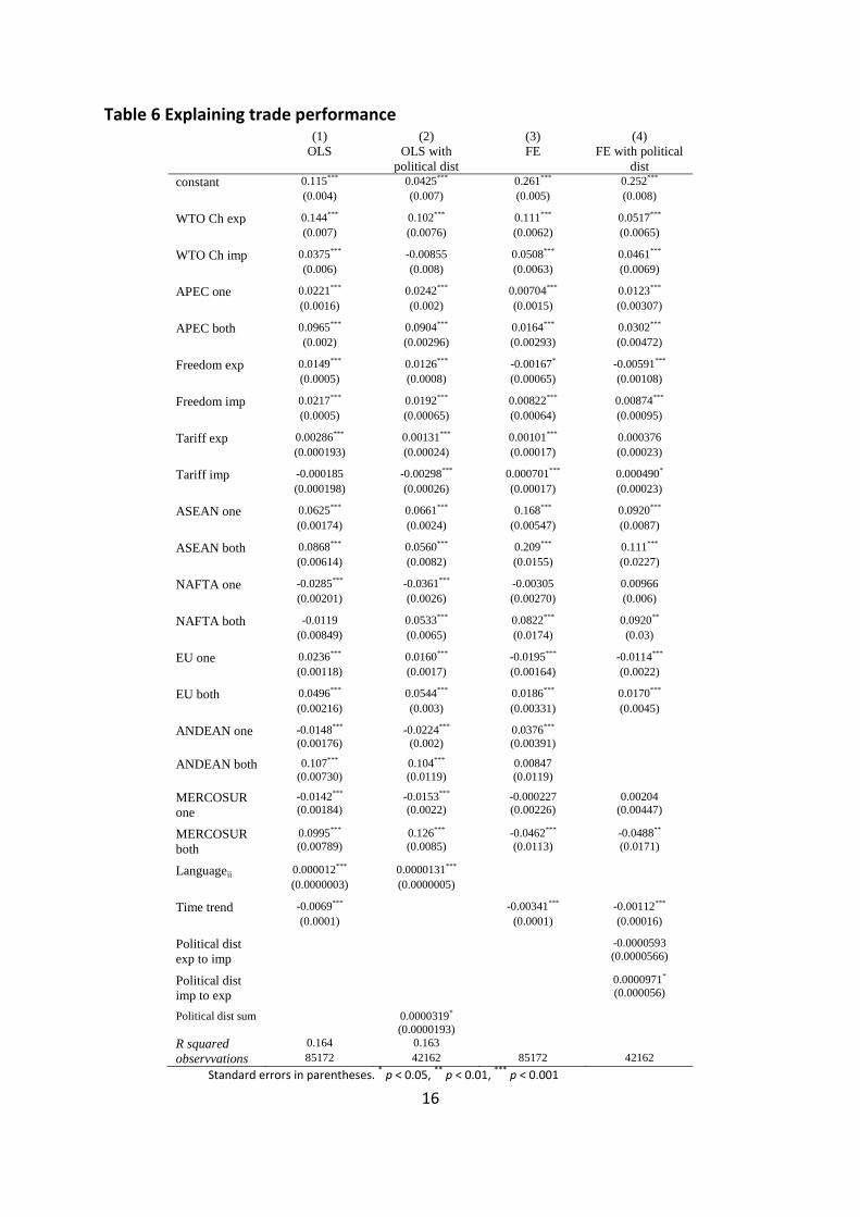
Table 6 Explaining trade performance (1) (2) (3) (4)
OLS OLS with
political dist
FE FE with political
dist
constant 0.115*** 0.0425*** 0.261*** 0.252***
(0.004) (0.007) (0.005) (0.008)
WTO Ch exp 0.144*** 0.102*** 0.111*** 0.0517***
(0.007) (0.0076) (0.0062) (0.0065)
WTO Ch imp 0.0375*** -0.00855 0.0508*** 0.0461***
(0.006) (0.008) (0.0063) (0.0069)
APEC one 0.0221*** 0.0242*** 0.00704*** 0.0123***
(0.0016) (0.002) (0.0015) (0.00307)
APEC both 0.0965*** 0.0904*** 0.0164*** 0.0302***
(0.002) (0.00296) (0.00293) (0.00472)
Freedom exp 0.0149*** 0.0126*** -0.00167* -0.00591***
(0.0005) (0.0008) (0.00065) (0.00108)
Freedom imp 0.0217*** 0.0192*** 0.00822*** 0.00874***
(0.0005) (0.00065) (0.00064) (0.00095)
Tariff exp 0.00286*** 0.00131*** 0.00101*** 0.000376
(0.000193) (0.00024) (0.00017) (0.00023)
Tariff imp -0.000185 -0.00298*** 0.000701*** 0.000490*
(0.000198) (0.00026) (0.00017) (0.00023)
ASEAN one 0.0625*** 0.0661*** 0.168*** 0.0920***
(0.00174) (0.0024) (0.00547) (0.0087)
ASEAN both 0.0868*** 0.0560*** 0.209*** 0.111***
(0.00614) (0.0082) (0.0155) (0.0227)
NAFTA one -0.0285*** -0.0361*** -0.00305 0.00966
(0.00201) (0.0026) (0.00270) (0.006)
NAFTA both -0.0119 0.0533*** 0.0822*** 0.0920**
(0.00849) (0.0065) (0.0174) (0.03)
EU one 0.0236*** 0.0160*** -0.0195*** -0.0114***
(0.00118) (0.0017) (0.00164) (0.0022)
EU both 0.0496*** 0.0544*** 0.0186*** 0.0170***
(0.00216) (0.003) (0.00331) (0.0045)
ANDEAN one -0.0148*** -0.0224*** 0.0376***
(0.00176) (0.002) (0.00391)
ANDEAN both 0.107*** 0.104*** 0.00847
(0.00730) (0.0119) (0.0119)
MERCOSUR
one
-0.0142*** -0.0153*** -0.000227 0.00204 (0.00184) (0.0022) (0.00226) (0.00447)
MERCOSUR
both
0.0995*** 0.126*** -0.0462*** -0.0488**
(0.00789) (0.0085) (0.0113) (0.0171)
Languageij 0.000012*** 0.0000131***
(0.0000003) (0.0000005)
Time trend -0.0069*** -0.00341*** -0.00112***
(0.0001) (0.0001) (0.00016)
Political dist
exp to imp
-0.0000593
(0.0000566)
Political dist
imp to exp
0.0000971* (0.000056)
Political dist sum 0.0000319*
(0.0000193)
R squared 0.164 0.163
observvations 85172 42162 85172 42162
Standard errors in parentheses. * p < 0.05,
** p < 0.01,
*** p < 0.001

17
The results in Table 6 explain trade performance and show that regional grouping variables,
language similarity and economic freedom help explain trade performance and trade
resistances. The variables of particular interest here are RTA and regional and multilateral
trade grouping variables.
Take the case of China’s accession to the WTO. China’s entry to the WTO increased both its
export and import performance by reducing resistances (except for imports in column (2) of
Table 6). These two variables have the largest estimated parameters and their effects on
trade performance are the largest among the trade policy related variables.
All regional groupings or RTA variables have a positive coefficient when both countries are
members, showing, as would be expected, that an RTA increases trade (and trade
performance) between members holding all else (such as distance, for example) constant.
The story diverges for regions when looking at the variables estimating the effect on trade
of an RTA or region when one county is a member and the other is not. The negative
coefficients on ‘NAFTA one’, ‘EU one’, ‘ANDEAN one’ and ‘MERCOSUR one’ mean that the
RTA membership or formation is trade diversionary.
A positive coefficient on the variables ‘ASEAN one’ and ‘APEC one’ means, for example, that
trade between an APEC member and a non-APEC country increased following the formation
of APEC or its membership of APEC.
The results show there is trade diversion from discriminatory regional trade blocs such as
NAFTA, MERCOSUR, ANDEAN, and the EU. APEC and ASEAN, on the other hand, show
increased trade among members as well as between members and non-members. There is
no evidence of trade diversion in the latter arrangements (Table 6).
There is also evidence that political distance affects trade. Model (2) does not have a time
trend as the inclusion of a time trend causes the political distance variable to be statistically
insignificant. In this model, the sum of directional political distance is statistically significant
at the 5 per cent level. Political distance from the importer’s perspective (events reported in
the importing country which are related to the exporting country) is also statistically
significant while political distance from the perspective of an exporter is not.
This asymmetry in the impact of political distance on trade is interesting and plausible. More
policy and political control is likely to be exercised over import activities than the activities
of exporters. A good example is the case of China-Taiwan trade where politically-driven
intervention that limits Chinese imports into Taiwan has persisted. On average it appears
that political distance does not matter for an exporter and increased uncertainty in dealing
with a buyer in another country does not affect the volume of trade. Trade seems to be
affected by how the importing country perceives the source country of the goods. These
results do not hold up when time trends are included or with other model specifications, for

18
example, using random effects instead of fixed effects estimation. While the evidence is not
so robust, however, political distance appears to affect trade.
The low R-squared of 16 per cent for these estimates confirms the consensus in the trade
literature that most of the frictions that limit the realisation of trade potential cannot be
easily measured. The trade performance results from Table 3 are a measure of all
resistances that limit the achievement of trade potential. The resistances identified in the
analysis here quantify roughly 16 per cent of their effect.
Language similarity, economic freedom, APEC membership and political distance are also
used to explain FDI performance. The choice of these variables is common in the literature
on trade and FDI models. The small number of dominant FDI source countries (especially
over the long time period under review) limits the number variables that can be included
and variables that might tell us whether there is investment diversion from RTAs cannot be
included. The OLS estimation results are presented in Table 7. The dependent variable is FDI
performance, found earlier and presented in Table 5. As in the case of the trade model, the
two stages (estimating performance and explaining performance) were estimated
separately with the performance results of Equation 2 being the dependent variable. The
binding constraint of data availability in the second stage was more restrictive in the FDI
case, compared to the case of trade, with the number of observations used in estimating
the frontier being 4,397 (Table 4) and the number for explaining the performance ranging
from 2,441 to 2,643 observations (Table 7).
The low R-squared is similar to that of the case of trade. The low R-squared is a reflection of
the significant proportion of resistances that are difficult to measure or even unobservable.
The low R-squared is also an indication of the difficulties that a simultaneous estimation of
the two stages might face7. The inclusion of a set of time dummy variables or a time trend
does not change the results in any significant way except to nullify the effect of host country
tariff level – not surprisingly confirming a linear trend in tariff reductions over time. The
economic freedom of the host country has a positive and significant effect, as would be
expected.
7 It is common to estimate the two stages of estimating and explaining the frontier simultaneously in stochastic
frontier analysis. If done separately, as in this study, a statistical distribution has to be chosen (with some
statistical tests) for the one sided residual term, u. If estimated simultaneously, the distribution is determined by
the variables in the second stage.

19
Table 7 Explaining FDI performance
Dependent variable: actual/potential FDI (1) (2)
Host freedom 0.0370*** 0.0355*** (0.00267) (0.00303) Languageij 0.0000156*** 0.0000149*** (0.00000211) (0.00000211) Host tariff 0.00242* 0.00179 (0.00112) (0.00118) Host APEC 0.0596*** 0.0444*** (0.00746) (0.00743) Political dist 0.000176*** (0.0000381) Lagged Political dist
0.000160*** (0.0000395)
Constant 0.131*** 0.159*** (0.0173) (0.0203) R-squared 0.1607
0.1252
N 2643 2441 Standard errors in parentheses
* p < 0.05,
** p < 0.01,
*** p < 0.001
Unlike the case for trade where a lot of trade is conducted on relatively short contracts, FDI
projects are a priori expected to be affected with a lag due to the inability to cancel
committed capital. Start-ups may be delayed or cancelled due to a worsening of political
climate. A lagged political distance variable is therefore included, with a one year lag
consistent with other findings. A one year lag is considered more appropriate than a two
year lag (Reuveny and Kang, 2003). This formulation has the added benefit of avoiding
causality running from economic distance to political distance8. There is evidence that
changes in economic relations influence political relations (Polachek, 1980; Mansfield and
Pollins, 2003). Improvements in a political relationship would not be expected to impact on
the economic relationship, and vice versa, immediately, but there is likely to be an effect
after a lag, as economic agents and foreign policy stances adjust. The results with a lagged
8 Other studies estimate simultaneous equations or use Granger causality type tests that account for, and often
find evidence of bi-directional causality (Reuveny and Kang, 2003; Mansfield and Pollins, 2003; Armstrong,
2009).

20
political distance variable are shown in Column 2 and these results do not vary significantly
from including political distance without a lag.
A measure of improving political relations helps explain an improvement in FDI performance
and hence an increase in FDI. This result is more robust than the case of the effect of politics
on trade (both in terms of statistical significance and sensitivity to different model
specifications). This finding can be explained by the fact that trade does not commit as
much in the way of resources as does the undertaking of FDI. Investing in another country
and building a plant or factory, often employing and procuring locally, is more sensitive to
political relations than arms length trade.
The analysis so far raises the question of how, on average, political distance has not had
significant effects on trade. This finding is for the average of the world sample and there are
obvious examples where political distance has dominated economic relations, such as
between India-Pakistan, the United States and North Korea and United States-Cuba. Why is
it that the economic interests seem to dominate political difficulties, despite these notable
exceptions? The following section revisits the Japan-China case mentioned above as it is an
example of how two major economic powers with episodes of rising political tensions in the
period under study, unresolved historical issues and regional rivalry, have nonetheless been
managed and it is a relationship that has seen the economic relationship flourish and
dominate.
The case of Japan and China
The relationship between Japan and China is a case in which there has been substantial
political distance from time to time (see Figure 1) yet the economic relationship, trade in
both directions and FDI from Japan, has seen consistently rapid growth.
Since normalisation of diplomatic relations in 1972 and the start of the economic
relationship in the modern era in 1978, political tensions have surfaced around disputed
territory in the South China Sea, Yasukuni shrine visits by Japanese political leaders, and
friction surrounding a rapidly rising China and the adjustments that both countries have to
make towards each other in this process, felt not only because of their respective economic
sizes but their proximity to each other.
With the backdrop of political tensions, the economic relationship boomed. Starting from a
very low base in 1978, in 2007 trade between Japan and China was the third largest bilateral
merchandise trade relationship in the world, in terms of exports and imports together,
behind the United States-Canada and United States-China trade relationships. Their
economies depend greatly on each other and China is Japan’s largest trading partner overall
and Japan is China’s second largest trading partner after the United States and the third
largest if the European Union (EU) is taken as a whole. Japan is the second largest source of
FDI into China after Hong Kong At the end of 2007 Japanese FDI stock in China was

21
approximately US$37 billion and FDI flows had averaged 37.8 per cent growth, year on year,
since 19859. This included average growth in the first half of the 1990s of almost 54 per cent
annually and 25 per cent from 2000 to 200410.
The trade performance results reported in this study and in Armstrong (2009) show that
Japanese trade with China generally performed above the world average between 1980 and
1990 and consistently above world average trade performance from 1990 to 2006. In 2006,
Japanese trade to China was achieving 42 per cent of its potential while trade from China to
Japan was achieving 44 per cent of its potential. This compares to the world average of 28
per cent at this time.
While adverse politics may have affected the economic relationships of other countries
significantly, for Japan and China the market dominated politics in the development of their
economic relationship.
There is no bilateral agreement between China and Japan that has underpinned the
development of their economic relationship in recent times. The Long Term Trade
Agreement of 1978 was directed to another purpose in another era before China had fully
committed to marketisation. Nor has the Bilateral Investment Treaty (BIT) of 1988 been the
main driver on the recent surge of Japanese FDI into China.
Rather, it is both countries commitment to the rules and norms of the international
institutional system embodied in the WTO that constrains the effects of bilateral political
tensions and has provided the foundations for the huge growth of their bilateral
relationship within the multilateral trading system.
China’s accession to the WTO in 2001 after 15 years of negotiation was a policy initiative
unlikely to be matched in the foreseeable future in terms of gains in international trade
(Drysdale and Song, 2000). The effect on Japanese trade with, and investment in, China was
profound as Japanese investors and business saw China as a real market for the first time
(Armstrong, 2009). Table 6 shows how large the impact of WTO accession was on Chinese
trade. But it was not only the event in 2001 that was important. The lead up to accession
shaped the way in which Japanese business dealt with China. In the lead up to accession,
China’s commitment to the global trading system and ultimately to a rules based institution
was the significant factor. Unilateral trade liberalisation and market oriented reforms from
1986 and throughout the 1990s, well documented in many studies such as Lardy (2002) and
Lin et al. (2003), meant that Japanese traders and investors could engage China confidently
and significantly ameliorate the effects of bad political relations.
9 Source: Japanese Ministry of Finance and OECD.Stat.
10 Source: Author’s calculations from Japanese Ministry of Finance FDI data.
http://www.mof.go.jp/english/files.htm

22
Chinese pro-reform leaders used the external institution of the WTO to increase the pace of,
and lock in, reforms. The reforms were wide-ranging and importantly secured financial, legal
and economic institution reform. In fact, no other member joining the WTO has given so
many concessions on the way to accession (Drysdale, 2000; Brandt et al., 2007). The
comprehensive reforms towards a more market-oriented system and commitments to
transparency constrained Chinese policy makers from political intervention in international
commerce across a very wide range of business activity (Garnaut and Huang, 2000).
Armstrong (2009) found that China’s commitment to the global trading system was the
reason that the political distance did not significantly affect the economic relationship
between Japan and China. In fact, he also finds evidence that the economic relationship,
with commitment to GATT, and later WTO entry, not only helped to insulate against the
political tensions, but allowed the economic relationship to constrain and shape the political
relationship.
The China-Japan political relationship is now underpinned by the large and significant
economic relationship. The scale and significance of the economic relationship is due to the
proximity of the two countries, their scales, complementarity in economic structures and
integration of both into the East Asia region (Armstrong, 2009). While the vagaries of
political distance have an effect on trade and FDI at the margins, the economic factors
dominate.
Conclusions
The analysis and argument in this paper suggest five important conclusions about
international trade and investment performance and international political relations.
The first is that multilateral institutions are very important in reducing economic and
political distance between trading partners. The impact of WTO membership on the
realisation of trade and investment potential is clear and measurable in the experience of
China’s accession to the WTO which lowered economic and political distance between China
and its economic partners. Specifically, the Japan-China example shows that, despite
recurring political tensions between these two important East Asian partners, China’s
accession to the WTO constrained their impact on bilateral trade and investment relations.
There is independent evidence that the circumstance of common membership of the WTO
has promoted the economic relationship between China and Japan to a point where that
relationship has impacted favourably on their political relationship.
The second is that while political relations do affect economic relations, their effect is not
important across the vast majority of trading relationships, especially for export activities
although less so for import activities. Generally politics affects trade at the margins beyond
the markets where governments have discretion in economic decision-making not subject to
international rules. Again, the presumption is that common membership of the multilateral
23
international institutions is an important element that constrains the impact of politics on
trade. Where the disciplines of the WTO do not apply and in cases where political behaviour
is not constrained by its rules and norms, politics are more likely to dominate economics.
The third is that the important effects of political relations on economic relations come in
today’s world via international investment rather than through international trade. The
nature of FDI, with its long lead-time, commitments in a domestic political setting and the
absence of a global regime that constrains political behaviour towards foreign investors
would appear to account for these differences between trade and investment relations. This
is an important conclusion for two reasons. FDI is now a very important element shaping
international economic integration. China and other emerging economies have recently
joined the industrial country investors abroad and the political problems associated with the
surge of Chinese investment abroad could complicate the international integration of what
is now one of the largest economies in the world (Drysdale and Findlay, 2009).
The fourth is that East Asian economies are leading trade and economic integration,
measured in terms of their trade and investment performance and their impact on global
trade and investment frontiers. East Asian economies, including ASEAN, have less resistance
to trade than the EU, North American and especially South Asian countries, in respect of
both inter-regional and intra-regional trade (Table 3). This is interesting and important in
the present context because trade and investment integration in East has taken place
without the framework of formal political ties or tight institutional arrangements between
the whole range of economies involved – absent ‘hard’ political associations – unlike in
Europe or North America.
Finally, of all the major regional groupings, APEC and ASEAN stand out as arrangements in
which there has been no trade diversion, unlike the other formal regional groupings of
NAFTA, EU, ANDEAM and MERCOSUR in which trade diversion is measurable (Table 6).
ASEAN and APEC are the most trade integrated regional groupings worldwide while ASEAN
is the most open FDI recipient, followed by the EU and APEC. ASEAN and APEC are also more
open to the rest of the world and not inward looking as evidenced by the trade diversion
found in other regional blocs. This may be no surprise as the design of both APEC and ASEAN
has been outward-looking. The story of APEC in particular is well known with policies of
liberalisation and reform, organised around the principle of open regionalism (a strategy
well-suited to the development, objectives and diversity of the Asia Pacific region). But
what may be more surprising is that, despite its ‘soft politics’ there is a measurable and
positive ‘APEC effect’ on members’ trade and investment with each other as well as on their
and investment globally.
24
Trade in the Asia Pacific is underpinned by open trading and investment regimes and low
border barriers to trade all encouraged by APEC members’ independent but collectively
endorsed commitments to these policy strategies.
This study highlights the priority that now needs to be given in this region to the regional
and international investment regime that comprehends regulatory and institutional issues
beyond the border if there is to be political security for the next phase of regional and
international economic integration. While the question is not addressed explicitly this paper
and it is a subject for another day, the evidence here does suggest that traditional regional
trade arrangements may not be the most efficacious instrument whereby to achieve these
objectives. What is clear is that, in future, economic flashpoint of political tension is more
likely to surround matters of investment than it is matters of trade.

25
References
Adams, R., Dee, P., Gali, J. and McGuire, G., 2003. 'The trade and investment effects of preferential trading arrangements - old and new evidence', Productivity Commission Staff Working Paper.
ADB, 2008. Emerging Asian Regionalism: A partnership for shared prosperity, Asia Development Bank, Philippines.
Anderson, J.E. and van Wincoop, E., 2003. 'Gravity with gravitas: a solution to the border puzzle', American Economic Review, 93(1):170–92.
Armstrong, Shiro, Peter Drysdale and Kaliappa Kalirajan, 2008. ‘Asian trade structures and trade potential: an initial analysis of South and East Asian trade’, EABER Working Paper, No. 28.
Armstrong, Shiro, 2007. ‘Measuring trade and trade performance: a survey’, Asia Pacific Economic Papers, No. 368.
— —, 2009. The Japan-China economic relationship: distance, institutions and politics, Canberra, Australian National University, Ph D thesis.
Baltagi, B., Egger, P. and Pfaffermayr, M., 2007, ‘Estimating models of complex FDI: are there third-country effects?’, Journal of Econometrics 140(1):260-281.
Blonigen, B.A., 2005. ‘A review of the empirical literature on FDI determinants’, NBER Working Paper No. 11299, National Bureau of Economic Research, May.
Brandt, L., Rawski, T. and Zhu, X., 2007. ‘International dimensions of China’s long boom: trends, prospects and implications, in China and the Balance of Influence in Asia, in W. Keller and T. Rawski (eds), University of Pittsburgh Press, Pittsburgh.
Coelli, T.J., 1996. 'A guide to FRONTIER Version 4.1: a computer program for stochastic frontier production and cost function estimation', CEPA Working Paper 96/07, University of New England.
Davies, R.B., 2008. ‘Hunting high and low for vertical FDI’, Review of International Economics, 16(2):250-67.
Dee, Philippa, 2007. ‘Multinational corporations and pacific regionalism’, in J.J. Palacios (ed.), Multinational Corporations and the Emerging Network Economy in Asia and the Pacific, Routledge.
Dowrick, S. and J. DeLong, B., 2003. ‘Globalisation and convergence’, in M.D. Bordo, A.M. Taylor and J.G. Williamson (eds), Globalization in Historical Perspective, University of Chicago Press, Chicago.
Drysdale, Peter, 1967. Australian-Japanese trade, Canberra, Australian National University. Ph D. thesis.
— —, 1988. International Economic Pluralism: Economic Policy in East Asia and the Pacific, Allen & Unwin, Sydney.
— —, 2000. ‘The implications of China’s membership of the WTO for industrial transformation’, in P.D. Drysdale and L. Song (eds), China's Entry to the WTO: Strategic Issues and Quantitative Assessments, Routledge, London.
Drysdale, Peter and Christopher Findlay, 2009. ‘Chinese Foreign Direct Investment in Australia: Policy Issues for the Resource Sector’, China Economic Journal, June and available at http://www.eastasiaforum.org/2008/09/04/chinese-investment-in-australian-resources/

26
Drysdale, Peter and Ross Garnaut, 1982. ‘Trade intensities and the analysis of bilateral trade flows in a many-country world: a survey’, Hitotsubashi Journal of Economics, 22(2):62-84.
Drysdale, Peter, Huang Yiping and Kaliappa Kalirajan, 2000. 'China's trade efficiency: measurement and determinants', in P. Drysdale, Y. Zhang and L. Song (eds), APEC and liberalisation of the Chinese economy, Asia Pacific Press, Canberra.
Drysdale, P.D. and Song, L., 2000. China's Entry to the WTO: Strategic Issues and Quantitative Assessments, Routledge, London.
Egger, P. and Pfaffermayr, M., 2004. ‘Distance, trade and FDI: a Hausman-Taylor SUR approach’, Journal of Applied Econometrics, 19(2):227-24.
Erramilli M.K. and D'Souza, D.E., 1995. ‘Uncertainty and foreign direct investment: the role of moderators’, International Marketing Review, 12(3):47- 60.
Garnaut, R. and Huang, Y., 2000. ‘China and the future of the international trading system’, in P.D. Drysdale and L. Song (eds), China's Entry to the WTO: Strategic Issues and Quantitative Assessments, Routledge, London.
Ghemawat, P, 2007, Redefining Global Strategy: Crossing Borders in a World Where Differences Still Matter, Harvard Business School Press, Boston MA.
Goldstein, J. S. 1992. ‘A conflict-cooperation scale for WEIS event data’, Journal of Conflict Resolution, 36:369-85.
Guiso, L., Sapienza, P. and Zingales, L., 2004. ‘Cultural biases in economic exchange’, NBER Working Paper No. 11005, National Bureau of Economic Research.
King, G., 2003. ‘10 million international dyadic events’, hdl:1902.1/FYXLAWZRIA UNF:3:um06qkr/1tAwpS4roUqAiw== Murray Research Archive [Distributor] http://gking.harvard.edu/homepage.html
Kumbhakar, S.C. and Knox-Lovell, C.A., 2000. Stochastic Frontier Analysis, Cambridge University Press, New York and Melbourne.
Lardy, N., 2002. Integrating China into the Global Economy, Brookings Institution Press, Washington DC.
Lin , Justin Yifu, F. Cai, Z. Li, 2003. The China miracle: development strategy and economic reform, Chinese University Press, Hong Kong.
Leamer, E., 1984. Sources of international comparative advantage MIT Press, Cambridge. Mansfield, E.D. and Pollins, B.M., 2001. ‘The study of interdependence and
conflict: recent advances, open questions, and directions for future research’. Journal of Conflict Resolution, 45:834-59.
— —, 2003. Economic Interdependence and International Conflict: New Perspectives on an Enduring Debate (eds), University of Michigan Press, Michigan.
Polachek, S. W. 1980. ‘Conflict and trade’, Journal of Conflict Resolution, 24:55-78. Reuveny, R. and H. Kang, 2003. ‘A simultaneous-equations model of trade, conflict, and
cooperation’, Review of International Economics, 11:279-95.

27
Data Annex
Capital stock
Following Leamer (1984) and common practice (see Dee, 2007 and Baltagi et al. 2007) the
capital stock is calculated using the perpetual inventory method. This is calculated using
gross fixed capital formation, K, at time t with the formula Kt = 2∑t+2t-2 It , where I is
investment with t sufficiently less than 1982, the period under study.
Trade frontier countries
Argentina, Australia, Austria, Bangladesh, Belgium and Luxemburg, Brazil, Bulgaria, Canada,
Chile, China, Colombia, Costa Rica, Cyprus, Denmark, Ecuador, Egypt, Finland, France,
Germany, Ghana, Greece, Honduras, Hong Kong, Hungary, India, Indonesia, Ireland, Israel,
Italy, Jamaica, Japan, Jordan, South Korea, Malaysia, Malta, Mauritius, Mexico, Netherlands,
New Zealand, Nicaragua, Nigeria, Norway, Pakistan, Panama, Paraguay, Peru, Philippines,
Poland, Portugal, Russia, Singapore, Slovakia, South Africa, Spain, Sri Lanka, Sweden,
Switzerland, Taiwan11, Thailand, Turkey, United Kingdom, United States, Uruguay,
Venezuela, an Vietnam.
FDI destination (or host) countries
Albania, Algeria, Argentina, Australia, Austria, Azerbaijan, Belgium, Belize, Benin, Bolivia,
Brazil, Bulgaria, Canada, Central African Republic, Chad, Chile, China, Costa Rica, Croatia,
Czech Republic, Denmark, Dominican Republic, Ecuador, El Salvador, Estonia, Finland,
France, Gabon, Gambia, Georgia, Germany, Ghana, Greece, Guatemala, Guinea, Hong Kong,
Hungary, Iceland, India, Indonesia, Iran, Ireland, Italy, Japan, Jordan, Latvia, Lithuania,
Luxembourg, Macau, Malaysia, Mauritius, Mexico, Morocco, Namibia, Netherlands, New
Zealand, Nicaragua, Norway, Pakistan, Panama, Papua New Guinea, Paraguay, Peru,
Philippines, Poland, Portugal, Romania, Russia, Singapore, Slovakia, Slovenia, South Africa,
South Korea, Spain, Sri Lanka, Sweden, Switzerland, Syria, Taiwan, Tanzania, Thailand,
Trinidad and Tobago, Tunisia, Turkey, UAE, UK, Ukraine, Uruguay, USA.
11
Trade and GDP data for Taiwan are from the International Economic Databank (IEDB), Australian National University, http://iedb.anu.edu.au/