the influence of attitudes and expectations on purchases · to purchase consumer durable...

This PDF is a selection from an out-of-print volume from the NationalBureau of Economic Research

Volume Title: Anticipations and Purchases: An Analysis of ConsumerBehavior

Volume Author/Editor: F. Thomas Juster

Volume Publisher: Princeton University Press

Volume ISBN: 0-87014-079-5

Volume URL: http://www.nber.org/books/just64-1

Publication Date: 1964

Chapter Title: The Influence of Attitudes and Expectations on Purchases

Chapter Author: F. Thomas Juster

Chapter URL: http://www.nber.org/chapters/c1034

Chapter pages in book: ( 140 - 165 )

CHAPTER 6

The Influence of Attitudes and Expectationson Purchases

Introduction

A MAJOR part of the existing research using consumer survey data has beenconcerned with relating attitudes and expectations to purchase behavior,both in time series and in cross sections. It is here that one finds thesharpest difference of opinion among researchers, both as to the interpre-tation of empirical results and the related question of usefulness inprediction.'PREVAILING HYPOTHESES

One view is that consumer attitudes (thought of as generalized feelings ofwell-being reflecting relative optimism or pessimism) are fundamentaldeterminants of spending and saving behavior and that both expectations(judgments about the course of events external to the household) andintentions (judgments about events internal to the household) are basicallyattitudes carrying a time dimension. Under this interpretation an appro-priate measure of consumer sentiment blends all three kinds of variables inthe same way as the characterization of a voter as prospectively Demo-cratic or Republican combines his opinions on philosophical questions, hisactual voting record in the past, his economic self-interest as reflected byincome status, etc.

1 On the one side are the works of Katona and Mueller: George Katona and EvaMueller, Consumer Attitudes and Demand, 1950—1952, Ann Arbor, Michigan UniversitySurvey Research Center, nd., pp. 51—61; Katona and Mueller, Consumer Expectations,1953—1955, Ann Arbor, Michigan University Survey Research Center, n.d.; Katona,"Business Expectations in the Framework of Psychological Economics," Expectations,Uncertainty, and Business Behavior, ed. M. J. Bowman, Ann Arbor, Michigan UniversitySurvey Research Center, 1958; Mueller, "Effects of Consumer Attitudes on Purchases,"American Economic Review, December 1957; Mueller, "Consumer Attitudes—TheirInfluence and Forecasting Value," The Quality and Economic SiJn(ficance of AnticipationsData, Princeton for NBER, 1960; and, most recently, Katona, The Powerful Consumer,New York, McGraw-Hill, 1960. Compare the foregoing with James Tobin, "Onthe Predictive Value of Consumer Intentions and Attitudes," in Review of Economics andStatistics, February 1959; Arthur Okun, "The Value of Anticipations Data in Fore-casting National Product," in Anticipations Data; Reports of Federal Reserve ConsultantCommittees on Economic Statistics, Joint Committee on the Economic Report, 84th Cong.,1st sess., 1955; F. Thomas Juster, Consumer Expectations, Plans, and Purchases: A ProgressReport, Occasional Paper 70, New York, NBER, 1959; Juster, "Prediction and Con-sumer Buying Intentions," American Economic Review, May 1960; and Juster, "ThePredictive Value of Consumers Union Spending-Intentions Data," in Anticipations Data.See also Peter De Janosi, "Factors Influencing the Demand for New Automobiles,"Journal of Marketing, April 1959; Lawrence R. Klein and John B. Lansing, "Decisionto Purchase Consumer Durable Goods," Journal of Marketing, October 1955; andLansing and Stephen B. Withey, "Consumer Anticipations: Their Use in ForecastingConsumer Behavior," Short- Term Economic Forecasting, Princeton for NBER, 1955.

140

INFLUENCE OF ATTITUDES AND EXPECTATIONS

Thus any factor reflecting greater (lesser) optimism will tend to increase(decrease) an individual's optimism index. Holding other attitudesconstant, households that report buying intentions or expect increasedincomes, ceteris paribus, will have higher index scores and should purchasemore than if they reported no buying intentions or expected decreasedincomes. Similarly, households with the same expectations and inten-tions but feeling "better off than last year" will have higher scores thanthose feeling "worse off," and will make more purchases. In a previouspublication I have labeled this viewpoint the "additivity" hypothesis, onthe grounds that its proponents argue that any attitude, expectation, orintention reflecting optimism will, ceteris paribus, result in a more favorabledisposition towards durable goods purchases, hence be associated with agreater amount of purchases.2

An alternative viewpoint is that attitudes, expectations, and intentionsshould be taken at face value. That is to say, expectations reflect thehousehold's judgment about the future course of events external to thehousehold; intentions, on the other hand, reflect tentative plans to under-take specified actions in the light of these judgments. Attitudes influenceboth expectations and the relation between expectations and intentions.In this view, purchases (actions) .are directly related to (or predicted by)intentions, modified by the incidence of unforeseen developments. Ihave previously labeled this viewpoint the "contingent-action" hypothesis.

Both of these views relate to the interpretation of responses to surveyquestions about attitudes, expectations, or intentions. Proponents ofboth views would agree that these responses are more than a simpleextrapolation of the respondent's experience. For if buying intentions orexpectations could themselves be predicted from the underlying "real"factors—data on stocks of goods, income, income change, occupation,etc.—measurement of consumer anticipations would be unnecessary.Indeed, many economists regard anticipatory variables as essentiallyepiphenomena, in that they contain no useful information over and abovethat provided by knowledge of the household's real situation—its leveland rate of change in income, demographic composition, and so forth.However, these economists would probably agree that the availabilityand timeliness of anticipatory data may well make them of considerable

2 See Consumer Expectations and "Prediction and Consumer Buying Intentions."The terminology is not intended to convey the impression that any or all possiblemeasures of sentiment carry equal weight or that none interact with others; it isdesigned to indicate that all measures of consumer sentiment that reflect optimismincrease index scores and, hence, are associated with higher rates of purchase, whileall measures that reflect pessimism have the reverse effect.

141

INFLUENCE OF ATTITUDES AND EXPECTATiONS

value in forecasting, even though they may be of no help in understandingor explaining behavior.

The test of these alternative viewpoints is clearly their ability to predictempirically observable phenomena. Appropriate tests are neither simpleto construct nor straightforward in interpretation. Take the relationbetween expected change in income, actual change in income, intentionsto buy durables, and actual purchases of durables. The additivityhypothesis predicts that expected change in income will be positivelyassociated with purchases, holding buying intentions and actual incomechange constant, since the larger the expected income increase the moreoptimistic the household; hence, the greater the amount of purchases. Onthe other hand, the contingent-action hypothesis predicts a negativeassociation between expected change in income and purchases, holdingintentions and actual income change constant; the larger the expectedincome increase the less agreeably surprised the household and, hence,the smaller the amount of purchases relative to buying intentions. Thethird possibility is that no association exists between expected incomechange and purchases, holding actual income change and past incomechanges constant, because expected change is nothing more than somekind of weighted average of past changes.

EXISTING EVIDENCE

These hypotheses can be tested with data from the CU surveys. Therelevant test indicates no statistically significant association between(expected change in income) and P (purchases of durable goods), holdingP (buying intentions) and iY (actual change in income) constant. Thisconclusion may be correct; but it is quite possible that the observed rela-tion is not significant because the actual relation is more complicated.For example, it is doubtful whether a single-valued estimate of expectedchange in income is an adequate measure of income expectations. If thestructure of such expectations is best described by a probability distribu-tion of the possible outcomes, both the mean and the dispersion of thedistribution are surely relevant. A single-valued response is presumablyto be interpreted as an estimate of the mean; but we obviously cannot besure of this. Further, no good measure of dispersion is available.3 As aconsequence, the difference between actual change in income and my

8 The basic data contain an estimate of the range of income changes regarded as"at all likely" by the respondent, but this estimate is not available for the time periodon which I have concentrated in this monograph.

142


single-valued measure of expected change may not be an accurate andunbiased measure of income surprise; and if it is not, the data cannotdiscriminate among the alternative hypotheses.

Previous investigations into the relation between durable goods pur-chases and anticipatory variables have generally provided support for theproposition that at least some anticipatory variables are associated withpurchases. In particular, buying intentions have always shown a strongstatistical relation to purchases in reinterview studies. On the other hand,a relatively weak or nil association has generally been found betweenattitudes or expectations and purchases.4 Tobin's results showed nosignificant net association between purchases and a number of variablesrepresenting attitudes and expectations; buying intentions were signifi-cantly related to purchases—actually, to the ratio of durables' purchasesto income. A study of the attitude index constructed by Katona andMueller showed a positive relation between attitudes and purchases net ofintentions, income, and age for the second half of 1954, but no significantrelation in the first half of 1955. In an earlier multivariate study, usingdichotomous variables for purchases and intentions to buy, Klein andLansing could find no important behavioral association between theattitude-expectation variables and purchases; buying intentions, as iscustomarily the case, were significantly related to purchases. In anotherearlier study, Lansing and Withey found significant associations betweenvarious attitudes or expectations and purchases, but the empirical testsgenerally involved little netting out of the effects of other variables.Lansing and Withey also found that the difference between expected andactual income change (income surprise) was significantly related topurchases of automobiles, net of intentions to buy.

The findings discussed here relate entirely to studies of behavioral differences amonga cross section of households. Studies of time series relationships between purchases ofdurables and expectational variables have been based on relatively few observations;more important for my purposes, the time series studies have not generally attemptedto test anticipatory variables net of a sophisticated (objective) model, largely becauseof the limited number of observations.

The available time series results are relatively more favorable to the hypothesis thatattitudes and expectations, as distinct from intentions to buy, arc related to purchasebehavior. Both intentions (P) and an index of attitudes (A) show significant relationsto purchases in some of these studies. Depending on the time period and the par-ticular choice of variables, it has been found that P is more important than A or viceversa (see Okun; and Mueller, "Consumer Attitudes—Their Influence and Fore-casting Value").

5 Mueller, "Effects of Consumer Attitudes on Purchases." In this study both pur-chases and intentions are modified yes-no constructs rather than dollar amounts, whichmay tend to weaken all the relationships somewhat.

143


SOME EXPLORATORY HYPOTHESES AND INVESTIGATIONS

In my judgment, existing studies of cross-section data have failed toprovide convincing evidence in support of any of the hypotheses describedabove. On the whole, I read the evidence as suggesting that both atti-tudes and expectations are essentially unrelated to purchase behavior,while buying intentions are strongly related. It is also possible, however,that these studies have failed to uncover relationships that really exist.Research on these problems has been handicapped to some degree by therelatively small sample sizes available. It is true that six or seven hundredcases are ample for multivariate analysis involving a large number ofexplanatory factors. But this sample size becomes less satisfactory if someof the variables are important for the young but not for the old, or forhouseholds with buying intentions but not for nonintenders, or if com-binations of extreme expectations or attitudes are much more importantthan moderate ones, etc.

On a priori grounds, there is some reason to suppose that the influenceof anticipatory variables on purchase behavior is not the same for allsubgroups in the population, that the effect of expectations and attitudesis not independent of buying intentions or other attitudes and expecta-tions, and so on. My object in the next two chapters is to explore some ofthese possibilities at greater length. In the balance of this chapter Ianalyze the interrelationships among a number of measures bearing onattitudes or expectations, aggregate buying intentions, and aggregatepurchases of durable goods. In the next chapter I summarize the resultsof an extensive multivariate regression analysis.

Purchases and Expectations

My first concern is with the relation between purchases and a cluster ofvariables that may be construed as either attitudes or expectations. Therelation between purchases and an index of attitudes has been examinedin a number of publications by Katona and Mueller.6 The componentparts of their attitude index have included variables such as expected andpast change in financial well being, expectations about general businessconditions, opinions about market conditions for durables (good-bad timeto buy durables), expectations about price changes plus an evaluation ofwhether these changes are "to the good" or "to the bad," and buyingintentions for durable goods. The index in their cross-section tests is

6 For example, see Consumer Attitudes and Demand, pp. 51—61; and Consumer Expecta-tions, p. 10.

144


essentially a scale of unweighted scores obtained from a trichotomousdistribution of respondents by each of the component variables.7 Thatis to say, respondents are assigned scores of 2, 1, or 0, depending onwhether they expect to be "better off," "the same," or "worse off" inthe future. If six such questions are included in the attitude index, scoresmay range from 12, corresponding to the maximum degree of optimism,to zero, the maximum degree of pessimism.

Two kinds of problems are involved in the construction of such indexes.First, at face value, some of the components are statements of expectations,i.e., they represent judgments about future events that may or may nothappen. The relation between optimistic expectations and purchasesmay or may not involve a positive association, since, as pointed out above,the net correlation between the two may depend on the difference betweenexpectations and outcomes. If so, optimistic expectations cannot beassigned a score until the corresponding outcome is known, although onthe average the appropriate score for a household with optimistic expecta-tions would be lower than that for a household with pessimistic expecta-tions if buying intentions are held constant. On the other hand, state-ments that seem to represent judgments about future events may reallybe nothing more than a general indicator of optimism, in which case theKatona-Muefler procedure is the appropriate one.8

The second is the problem of weighting, both within and between thevariables that constitute the index. A trichotomous (2,1,0) scale forbetter-same-worse or up-no change-down supposes that the differencebetween better-worse is just twice as large as that between better-same orworse-same, and that households reporting "better" are distributed at theupper end of the true optimism scale in the same way as those reporting"same" are distributed in the middle part of the scale and those reporting"worse" at the lower end of the scale. Similar assumptions must hold forcomparisons across the variables that are index components.

For the most part the CU data do not lend themselves to a thoroughexamination of this range of problems, since the surveys were not designedfor exhaustive tests of this nature. However, enough information isavailable to explore the question of whether the relation between attitudes(or expectations) and subsequent purchases is suitably described by atrichotomous classification of the sort just discussed.

7 The rationale for the procedure is described in Katona and Mueller, ConsumerExpectations.

8 In practice this difficulty only arises when both buying intentions and expectationsare components of the index, since the possible negative association between expecta-tions and purchases would be observed only when intentions are held constant.

145


EMPIRICAL RESULTS

To examine the question of appropriate weighting I use responses to threevariables that relate to household attitudes9 These questions concern(1) actual change in family income over the past year; (2) expected changein family income during the next year; (3) expected change in generalbusiness conditions during the next year. All three questions wereaccompanied by a five-point scale: large increase (improvement), smallincrease (improvement), no change, and small or large decreases (deteri-oration). In addition, respondents could check categories labeled"don't know," "too uncertain to guess," or "other," depending on theparticular question.

Alternative methods of scoring these responses were utilized. In thefirst, 1 = increase (large or small) 2 = no change, and 3 = decrease

(large or small); households with any other responses were excluded fromthe sample. Hence, the index scores range from a maximum of 9 (themost pessimistic group) to a minimum of 3 (the most optimistic group).For husband-wile households with heads between twenty-five and thirty-four years of age, the weighted average number of durable goods pur-chased by each index score group is shown in Table 27.

This index, composed of three trichotomous classifications within eachof three variables, has a highly significant relation to purchases. A one-way analysis of variance on the cell means yields an F ratio of 3.49,significantly different from unity at the 0.01 level. The pattern of the cellaverages is consistent—except for the group with an attitude score of 7—with the proposition that favorable or optimistic attitudes are associatedwith relatively high purchases; pessimistic attitudes, with relatively lowpurchases. While it is true that those with optimistic attitudes tend tohave relatively higher incomes than those with pessimistic attitudes,adjusting for the influence of family income weakens but does not alterthe above relationship; differences in purchases among: attitude classes arestill significant at the 0.01 level, holding family income constant. The

For present purposes I bypass two problems of considerable importance. First,are these questions really about attitudes, or about expectations, or about simple fact?Secondly, are these the appropriate questions to use in order to construct thc bestpossible index of attitudes? Both are obviously significant questions. I put them asidenow because the question of appropriate weighting is important regardless of whetherthe index really measures fact, diffuse attitudes, or expectations, and regardless ofwhether the best index should include more or different components. These par-ticular questions happen to be available, and I do not claim that they constitute anoptimal combination of variables that relate to (or measure) household optimism orpessimism.

146

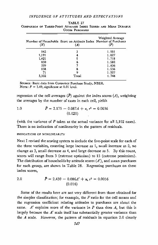
INFLUENCE OF ATTITUDES AND EXPECTATIONSTABLE 27

COMPARISON or THREE-POINT ATTITUDE INDEX SCORES AND MEAN DURABLEGOODS PURCHASES

Weighted AverageNumber of Households Score on Attitude Index Number of Purchases

(N) (A) (P)

942 3 1.951

1,191 4 1.8271,421 5 1.718

830 6 1.582

509 7 1.636

138 8 1.536

71 9 1.507

5,102 Total 1.748

SOURCE: Basic data from Consumer Purchase Study, NBER.NOTE: F = 3.49, significant at 0.01 level.

regression of the cell averages (P) against the index scores (A), weightingthe averages by the number of cases in each cell, yields

1.0 P = 2.175 — 0.087A + u, r2 = 0.0036

(0.020)

(with the variance of P taken as the actual variance for all 5,102 cases).There is no indication of nonlinearity in the pattern of residuals.

INDICATIONS OF NONLINEARITY

Next I revised the scoring system to include the five-point scale for each ofthe three variables, counting large increase as 1, small increase as 2, nochange as 3, small decrease as 4, and large decrease as 5. By this count,scores will range from 3 (extreme optimism) to 15 (extreme pessimism).The distribution of households by attitude scores (A'), and mean purchasesfor each group, are shown in Table 28. Regressing purchases on theseindex scores,

2.0 P = 2.439 — 0.086A' + u, r2 = 0.0056

(0.016)

Some of the results here are not very different from those obtained forthe simpler classification; for example, the F ratio for the cell means andthe regression coefficient relating attitudes to purchases are about thesame. A' explains more of the variance in P than does A, but this islargely because the A' scale itself has substantially greater variance thanthe A scale. However, the pattern of residuals in equation 2.0 clearly

147

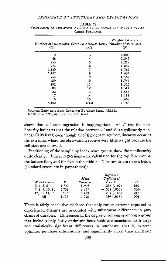
INFLUENCE OF ATTITUDES AND EXPECTATIONSTABLE 28

COMPARISON OF FIVE-POINT ATTITUDE INDEX SCORES AND MEAN DURABLEGOODS PURCHASES


(N) (A') ()2 3 4.000

48 4 2.542

253 5 2.217924 6 1.887

1,130 7 1.762

1,162 8 1.669

764 9 1.569

489 10 1.744

192 11 1.526

88 12 1.511

22 13 1.545

17 14 1.118

6 15 0.667

5,102 Total 1.748

SOURCE: Basic data from Consumer Purchase Study, NBER.NOTE: F = 3.95, significant at 0.01 level.

shows that a linear regression is inappropriate. An F test for non-linearity indicates that the relation between A' and P is significantly non-linear (0.05 level) even though all of the departures from linearity occur atthe extremes, where the observations receive very little weight because thecell sizes are so small.

Partitioning of the sample by index score groups show the nonlinearityquite clearly. Linear regressions were calculated for the top four groups,the bottom four, and the five in the middle. The results are shown below(standard errors are in parentheses):

RegressionMean Coefficient of

A' Index Scores N Purchases P on A' r23,4,5,6 1,232 1.993 —.386 (.107) .0107,8, 9, 10, 11 3,737 1.679 — .038 (.030) .0004

12,13,14,15 133 1.429 —.209 (.166) .012All 5,102 1.748 —.089 (.016) .006

There is fairly conclusive evidence that only rather extreme expected orexperienced changes are associated with subsequent differences in pur-chases of durables. Differences in the degree of optimism among a groupthat includes only fairly optimistic households are associated with largeand statistically significant differences in purchases; that is, extremeoptimists purchase substantially and significantly more than moderate

148


optimists. The same is true of the association between differences in thedegree of pessimism among pessimists and differences in purchases,although these differences are not statistically significant partly becausethe sample contains relatively few pessimistic households. On the otherhand, equally wide (index score) differences in the degree of optimism orpessimism among those who are moderately one or the other (or completelyneutral) are not associated with significant differences in purchasesdespite the very large sample of households in this category; for themoderate group, differences in purchases per scale unit are onlyabout one-tenth as large as for either of the other two groups. Thus, all of theobserved significant relationship between index scores and purchases isapparently due to the behavior of households at the extremes of the indexscore range.

SOME NONLINEAR FUNCTIONS

Further experiments involved fitting some nonlinear functions to thesedata. Nonlinear scores were introduced by assigning values of 1, 4, 5,6, and 9 in place of the 1, 2, 3, 4, 5 weighting underlying the Table 28classification. The resulting scores range from 3 to 27. I then estimatedthe three regressions shown below:

3.0 P=bo+bjT+u,where T is the rescaled A' index.

4.0 P=bo+biT'+u,/1 1where T T30— T

5.0 P = b0 + b1T + b2T2 + b3T3 + .

Since equation 3.0 is simply a linear version of the nonlinear scale(1,4,5,6,9) described above, it is a moderately nonlinear regression.Differences in behavior among those expecting or experiencing largechanges, small changes, no change, etc., are presumed to be adequatelyreflected by the ratios of 1:4: 5: 6: 9; that is, those anticipating largeincreases are expected to show three times as much of a difference inpurchases, relative to those anticipating small increases, as those antici-pating small increases relative to those anticipating no change or no changerelative to small decreases. Regressions 4.0 and 5.0 reflect the generalrelationship shown above—that the larger and more consistent are anti-

149


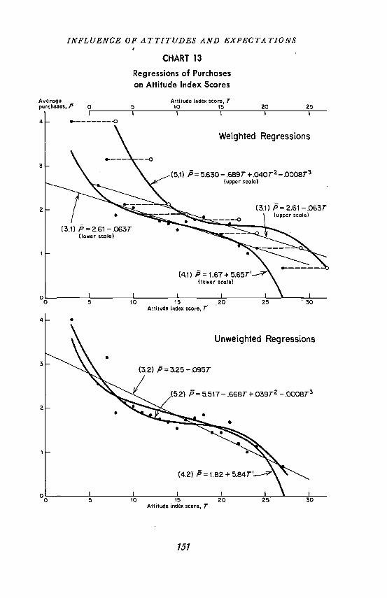
cipated changes the greater wili'be the difference in purchases. Equation4.0 imposes symmetry, in that the shape of the curve from 0 to 15 (thescale midpoint) must be a reversed (mirror) image of the shape in the15-to-30 range; equation 4.0 also imposes a slope of infinity at scale valuesof 0 or 30. Equation 5.0 does not contain any of these constraints; itcould show that optimism and purchases are positively related in severalsegments of the scale and negatively related or unrelated elsewhere. Thecomputed regressions, weighted by cell frequencies, are plotted in the toppanel of Chart 13 and summarized below.

3.1 P = 2.608 — 0.0632T + u,r2 = 0.0067

(0.011)4.1 P = 1.670 + 5.6467T' + u, r2 = 0.0075

(0.910)5.1 P = 5.630 — 0.689T + 0.040T2 — 0.0008T3 + R2 = 0.0093

(0.191) (0.013) (0.0003)

Unweighted regressions based entirely on the cell means, shown below,are plotted in the lower panel of Chart 13.

3.2 P = 3.25 — 0.095T+ u, r2 = 0.746

(0.012)4.2 P = 1.818 + 5.845T' + u, r2 = 0.840

(0.557)5.2 P = 5.517 — 0.668 + 0.039T2 — 0.0008T3 ± u, R2 — 0.850

(0.330) (0.024) (0.0005)

Chart 13 shows the computed regressions; the observed points areshown as heavy dots. The top panel (with the weighted regressions)shows the linear 3.1 equation and equation 4.1 plotted against the lowerscale for attitude scores. The linear regression and equation 5.1 areplotted against the upper scale for attitude scores, and several of theobserved points are redrawn as hollow dots. The two nonlinear functionsare so close together in the middle range that it would be hard to tell themapart if both were shown on the same scale.

These results are quite interesting in several respects. First, bothequations 4.1 and 5.1 constitute a significant improvement over equation3.1; allowing for the loss of additional degrees of freedom, the F ratio forthe additional explained variance is significant (0.05 level) for bothweighted and unweighted versions of 4.0 and 5.0. Secondly, the differ-ences between the weighted and unweighted regressions are rather striking.

150


CHART 13

Regressions of Purchaseson Attitude Index Scores

151

Average —

purchases, PAltitude Index score, r

tO 15T T

Weighted Regressions

P= 5.630 - .689T +.040T2—.0008T3(upper scale)

Attitude index score, T

.

4

3

2

(3.2) P=3.25—.095T

Unweighted Regressions

(5.2) P= 5.517 — .668T +.039T2 — .0008T3

S

Attitude index score, T


Regression 3.2 (unweighted) has .a much larger (absolute) slope than 3.1(weighted) because the extreme observations, which are well above theregression line at the optimism end of the scale and well below at thepessimism end, are given equal weight instead of a weight proportional tocell size. But the apparent fit of the 4.0 and 5.0 regressions is practicallythe same in both weighted and unweighted versions. Since the weightsare arbitrary in the sense that they reflect the particular sample beingsurveyed, the unweighted regressions may be more meaningful as ameasure of behavior for households with different characteristics providedthat sampling errors in the cell means can be neglected. The fact thatthese regressions show the same results either weighted or unweightedindicates to me that they probably constitute a substantially accuratedescription of the true relationship between these variables.

Finally, equation 5.0 turns out to have a slope of close to zero in themiddle range of attitude scores in both weighted and unweighted versions.As noted before, this regression is not constrained at all. But it is almostsymmetrical about the scale midpoint, with a slope that indicates verylittle difference in purchases over the range of attitude scores from about12 to 20—out of a total range of scores from 3 to 27. Both nonlinearfunctions have flatter slopes than the linear function in the middle of thescale, indicating that differences in moderate attitudes are not as useful indiscriminating between households with relatively high or low purchaserates as are differences in extreme attitudes.

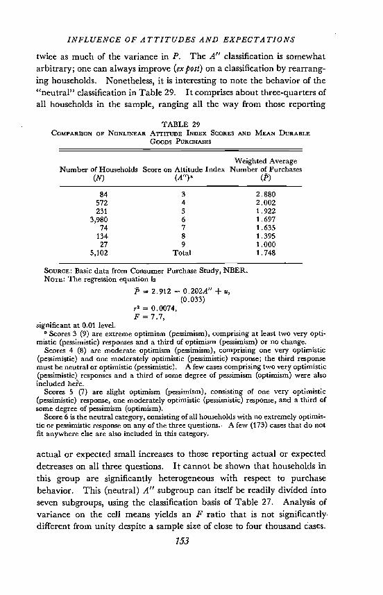
The above results suggest that differences in purchase behavior aredominated by the behavior of households expecting or experiencing largechanges. Further tests of this hypothesis can be constructed. I dividedthe sample into the same number of groups as in the A index (Table 27),but defined the groups on the assumption that expecting or experiencinglarge changes is the dominant cause of differences in purchases. Thus Ilumped together all households that did not report any large actual orexpected change on all three questions, and defined this group as havingneutral attitudes. The remaining households were divided into threegroups of optimists and three of pessimists,'° depending on the relativebalance of optimistic and pessimistic replies on the three questions; thecell averages resulting from this classification (A") are shown in Table 29.The same tests were then run on this as on the Table 27 classification.

The classification in Table 29 is clearly superior to that in Table 27;the F ratio is about twice as high, and the A" index scores explain about

"A small residual group that had a pattern of optimism-pessimism-no change wasalso included in the neutral group.

152


twice as much of the variance in P. The A" classification is somewhatarbitrary; one can always improve (expos€) on a classification by rearrang-ing households. Nonetheless, it is interesting to note the behavior of the"neutral" classification in Table 29. It comprises about three-quarters ofall households in the sample, ranging all the way from those reporting

TABLE 29COMPARISON OF NONLINEAR ATTITUDE INDEX SCORES AND MEAN DURABLE

GooDs PURCHASES


(N) (A")a (P)

84 3 2.880572 4 2.002231 5 1.922

3,980 6 169774 7 1.635

134 8 1.39527 9 1.000

5,102 Total 1.748

SOURCE: Basic data from Consumer Purchase Study, NBER.Nora: The regression equation is

P = 2.912 — 0.202A" + u,(0.033)

= 0.0074,F = 7.7,

significant at 0.01 level.R Scores 3 (9) are extreme optimism (pessimism), comprising at least two very opti-

mistic (pessimistic) responses and a third of optimism (pessimism) or no change.Scores 4 (8) are moderate optimism (pessimism), comprising one very optimistic

(pessimistic) and one moderately optimistic (pessimistic) response; the third responsemust be neutral or optimistic (pessimistic). A few cases comprising two very optimistic(pessimistic) responses and a third of some degree of pessimism (optimism) were alsoincluded he?e.

Scores 5 (7) are slight optimism (pessimism), consisting of one very optimistic(pessimistic) response, one moderately optimistic (pessimistic) response, and a third ofsome degree of pessimism (optimism).

Score 6 is the neutral category, consisting of all households with no extremely optimis-tic or pessimistic response on any of the three questions. A few (173) cases that do notfit anywhere else are also included in this category.

actual or expected small increases to those reporting actual or expecteddecreases on all three questions. It cannot be shown that households inthis group are significantly heterogeneous with respect to purchasebehavior. This (neutral) A" subgroup can itself be readily divided intoseven subgroups, using the classification basis of Table 27. Analysis ofvariance on the cell means yields an F ratio that is not significantlydifferent from unity despite a sample size of close to four thousand cases.

153


CONCLUSIONS

On the whole, the evidence strongly suggests that extreme combinationsof attitudes or expectations are significantly related to purchase behavior,while moderate ones are apparently either unrelated or quite weaklyrelated. These relationships hold for a sample of relatively young familieswith the head of household between twenty-five and thirty-four years ofage. It should be noted, however, that the same pattern was not foundamong older families with heads between forty-five and sixty-four. Herethe data show that the relation between purchases and attitudes is rela-tively weak in general, although it is statistically significant for a linearclassification like that in Table 28. Further, there is no evidence at allthat a nonlinear classification such as A" is an improvement. On theother hand, there is no indication that the neutral group in the A" classi-fication for these older families, comprising close to three thousand cases,is significantly heterogeneous, even though the range of (linear) attitudescores covers fully half the range of the entire classification. In sum, Iwould regard the evidence on the importance of extreme and the unim-portance of moderate attitudes and expectations as strongly suggestivethough not wholly conclusive.

Purchases, Buying Intentions, and "Surprises"

I turn now to the relation among expectations, outcomes, intentions, andpurchases to find out whether surprises or whether expectations themselvesseem to be associated with purchases net of intentions to buy. The rele-vant classifications can readily be constructed, since data are available onboth expected and actual income change on a five-point scale ranging fromlarge increase to large decrease. Thus, income surprise can be defined asactual change minus expected change (Y — i2), where both Y and

range from 5 (large increase) to I (large decrease).According to the contingent-action hypothesis, discussed earlier in this

chapter, LsY — should be positively correlated with purchases, holdingbuying intentions constant; groups of households with relatively large(algebraic) values of Y — I' should buy more, relative to intentions,than those with relatively small values of the surprise variable. Aspointed out earlier, this measure of income surprise may be seriouslydeficient, because it depends wholly on a single-valued estimate of II anddoes not take any account of dispersion. According to the additivityhypothesis, also discussed earlier, optimistic expectations should beassociated with relatively heavy purchases net of buying intentions.

154


Since increases in income would also tend tobe associated with relativelyheavy purchases, the additivity hypothesis can be interpreted as sayingthat iY + ? should be positively correlated with P net of intentionsbecause both components have a positive association.11

SOME PREVIOUS EVIDENCE RE-EXAMINED

Extensive tests of the relation between purchases (F), buying intentions(P), and expected and actual change in income (? and EsY, respectively)failed to uncover any systematic net relation between P and the incomeexpectation variable. Some of my investigations in earlier stages of thisproject'2 had indicated that, using grouped data, an equation of the form

6.0 P/P= bo+biLY+b2L?+uyielded negative coefficients for ? and positive ones for iY that werestatistically significant. Thus, favorable income surprises appeared to beassociated with high purchases relative to intentions, as predicted by thecontingent-action hypothesis, while expectations themselves were asso-ciated with low purchases relative to intentions, contradicting the addi-tivity hypothesis. The same paper also reported that an equation of theform

6.1 P = b, + b,P + b2Y + b3? + uyielded nonsignificant coefficients for both expected and actual change inincome. The negative results of equation 6.1 were attributed to thedifferential impact of expected income change on purchases by intendersand nonintenders. The argument essentially is that expectations aboutincome change may be acting as a probability-scaling device for thosereporting zero buying intentions, while for those reporting nonzerointentions probability-scaling is dominated by the income-surprise role ofincome expectations. Hence, the net relation between purchases andexpectations is positive for nonintenders, negative for intenders, and maynot show up at all if both groups are averaged.

This explanation for the negative results of equation 6.1 may well becorrect. However, the results of equation 6.0 clearly do not support thecontingent-action hypothesis, since they are largely, if not entirely, dueto a spurious correlation between expected change in income and the

11 Blending both hypotheses, one could argue that all three variables—Y, Y, andY — Y—ought to have a positive association with purchases net of buying intentions.

In this case the relation between Y and P becomes impossible to predict, since itdepends on whether the optimism or the surprise effect of i V predominates.

"See "Prediction and Consumer Buying Intentions," pp. 604—617.

155


ratio of purchases to intentions.'3 The spurious element in the correlationdisappears if purchases and intentions are introduced as separate varia-bles.'4 Hence, the empirical tests that use group averages do not showany relation at all between the income change variables and purchases,net of buying intentions.

SOME EXPERIMENTAL RESULTS

The apparent lack of association between purchases and either expecta-tions or surprises net of buying intentions is also shown by the results of an

I am indebted to George Katona for calling my attention to the spurious relationbetween income surprise and the ratio of aggregate purchases to aggregate intentions.

14 explanation is as follows: We are interested only in whether households withpessimistic (optimistic) income expectations, holding income change constant, tend tobuy more (less) relative to intentions than those with optimistic (pessimistic) expecta-tions. If this turns out to be the case, it follows that agreeable or favorable surprisesare positively correlated with purchases, given intentions. Let us take a group ofhouseholds with varying expectations about income change, all of whom experiencedno change in income. Some fraction of each income expectation class will reportbuying intentions for each of the commodities on the list, and another fraction willreport that they have purchased; the dependent variable in equation 6.0 is the ratio ofthese two fractions, summed across commodities. That is,

P = Ex, andP = Ep; hence

P/P = Ex/Ip.But it has been shown above that, using the notation of Chapters 2 and 3, x =

pr + (1 —p)s;hence— E[pr + (1 — p)s] — Epr Es(l — p)

I—

Suppose, for the sake of argument, that income surprise is completely unrelated tobehavior, i.e., that the contingent-action hypothesis has no empirical content. Itfollows that r (the fraction of intenders who buy) and s (the fraction of nonintenderswho buy) will be the same for each of the income-surprise classifications; for if incomesurprise has no relation to behavior, it clearly will not influence either r or s. Butfrom the formulation above it is apparent that even if both r and s are invariant withrespect to income surprise, P/P will be related to surprise provided that p (the fractionof the group reporting intentions) happens to be related. It is known (empirically)that p is correlated with income expectations; the more optimistic are expectations, thegreater the fraction of households that report intentions. But holding actual change inincome constant, expectations must be inversely correlated with income surprise;hence, a group of households with unfavorable income surprises (i.e., optimisticexpectations) will have a higher value of p than a group with favorable surprises (i.e.,pessimistic expectations). The higher the value of p, holding r and s constant, thelower the ratio of P to P. As a consequence, households with unfavorable incomesurprises will show relatively low ratios of P to P because of differences in p, even thoughr and s may be identical for all groups.

This spurious element is powerful enough to force a statistically significant negativecorrelation between £Y and P/P. Suppose, for example, that r = 0.5 and s = 0.2,and that both r and s are the same for all commodities and also for optimists andpessimists. Suppose further that p is 0.3 for optimists, 0.2 for pessimists. Then P/Pfor optimists is 0.5 + [0.2(0.7/0.3)] = 0.97; for pessimists, P/P equals

0.5 + [0.2(0.8/0.2)] = 1.30.

155


extensive multiple correlation analysis, using individual households asthe unit of observation. The sample was stratified into relatively homoge-neous life-cycle groups, since it seemed likely that these variables mighthave differential effects on behavior for young-old, married-unmarried,etc. The following regressions were computed for different life-cyclegroups and for several of the intentions questions.

7.0 P = b0 + b1P+ b2Y+ b3?+ + u8.0 P = b0 + b1P+ b2(iY— J) + . + u

7.1 P=bo+b1P+b2Y+b3+b4ZM++u8.1 P+bo+biP+bs(LY—i+baZ(Y—i1')++uIn 7.1 and 8.1, Z = 1 when P 0; otherwise 2' = 0.

On the whole, the results were discouraging. Significant positivecoefficients for income surprise or significant negative coefficients forincome expectations appeared on occasion; but so did significant coeffi-cients with the opposite sign; and the bulk of the and Y —coefficients were ionsignificant despite sample sizes of typically over sevenhundred cases. If any systematic pattern was present in these coefficients,it was not readily apparent.

The lack of positive results could be due to several factors. First,either expectations, or surprises, or both may in fact be unrelated tobehavior. Secondly, a relation between expectations and purchases mayactually exist but cannot be observed unless a good measure of the dis-persion of expectations can be included in the analysis; as pointed outbefore, my data do not have such a measure. Finally, it is possiblethat the relation among expectations, outcomes, purchases, and buyingintentions depends on the level of purchase probability associated withintentions.

As regards the second point, correspondence between analytical con-cepts and the survey variables used to represent them is not necessarilyclose. For example, we speak of testing to determine whether or not sub-jectively held expectations about income are related to purchase behavior.But we are not really testing income expectations per Se; rather, the testvariable consists of responses to a particular question bearing on incomeprospects. If the empirical results indicate that subjective income expec-tations are unrelated to purchases, it may mean only that the particularquestion is an unsatisfactory representation of expectations. Incomeexpectations (properly measured) undoubtedly have a bearing on decisionsto buy durable goods, although subjective statements concerning incomeprospects may not be useful.

157

INFLUENCE OF ATTITUDES AND EXPECTA TIONS

In a way, empirical analysis of survey data is an attempt to find particu-lar questions that are capable of being used as proxies for analyticallyrelevant variables. In some cases it is known from theory that a factoris related to behavior in a particular way, and it is required to find outif the relationship is strong or weak, or whether it has the same influencein all groups. If survey responses that purport to represent this factor aretested and no relationship is found, the presumption is that the particularquestion is poorly suited. In other cases it may not be known whetherthe measuring rod is faulty or whether there simply is no importantbehavioral relationship present.

As regards the third point, let us now take a closer look at the relationbetween purchases, intentions to buy, and deviations between expectedand actual income changes (surprises). It was argued above that thosewith favorable or agreeable surprises ought to purchase more, relativeto intentions, than those with no surprises; by the same token, those withunfavorable or disagreeable surprises ought to purchase less, relative tointentions, than those with no surprises. The empirical evidence didnot support the existence of such a relation, either because the relation infact does not exist or because the measure of surprise is deficient.

But it can also be plausibly argued that these relations depend on thespecification of a "buying intention," in particular, on the purchaseprobability associated with a statement of intention to buy. Supposethat two kinds of intentions are reported by households—those vith'avery high purchase probability and those with a probability that is rela-tively low but significantly higher than zero. Let us designate high-probability buying intentions as "standard" (P), low-probability intentionsas "contingent" (P).'5 It could be argued that favorable surprises willhave comparatively little influence on the ex post probability of purchaseby households with standard (P) intentions because ex ante purchaseprobability is already very high;" unfavorable surprises, on the otherhand, might have a relatively strong effect on ex post purchase probabilityfor these households. High ex ante purchase probability must have beenpredicated on a set of expectations, at least one of which (income expecta-

1 designation is the same as that used in Chapter 5 for a similar purpose.cx ante purchase probability I have in mind the respondent's subjective purchase

probability as of the survey date; by cx post purchase probability, his subjective proba-bility as of the survey date if he had known with certainty the actual course of externalevents during the forecast period. Thus, cx ante and expost purchase probability are thesame for a respondent with perfectly certain expectations about external events all ofwhich occur. Ex ante probability is greater than cx post probability for a respondent whoexperiences unfavorable (and unforeseen) changes; and the reverse is true for a respond-ent who experiences favorable (and unforeseen) changes during the forecast period.

158


tions) has resulted in disappointment for the group experiencing unfavora-ble or disagreeable surprises. As a consequence, some households in thisgroup may be unable or unwilling to purchase in accordance with theirex ante probabilities.

A similar dichotomy may be present with respect to the relation amongpurchases, contingent intentions (Ps), and surprises. Favorable surpriseswould be expected to have an especially strong influence on the purchasesof households with contingent intentions, since the intentions themselvesmay have been contingent (ex ante) precisely because income had not beenexpected to change in as favorable a way as it actually did. On theother hand, the groups with no surprises or with unfavorable ones mightbe expected to show the normally weak relation between P and P; sincethe relation is weak to begin with, those with unfavorable surprises mayact in much the same way as those with no surprises.

In sum, the association between purchases and standard intentions maybe significantly weaker for the unfavorably surprised than for others, andmay be somewhat stronger for the favorably surprised than for the no-sur-prise group. The relation between purchases and contingent intentionsmay be especially strong for the favorably surprised, perhaps somewhatweaker for the unfavorably surprised than for the no-surprise group.

It must be remembered that these analytical concepts are very imper-fectly represented by the data. In particular, lacking a measure of thedispersion of expectations, the surprise variable is suspect. As notedbefore, mean expected change, which is to be compared with reportedchange, is hardly an adequate description of expectations. Further, aclean distinction between standard and contingent plans, as these termsare used above, is lacking.

As a first step, I separated out households with agreeable or disagreeableincome surprises and estimated regression coefficients for purchases onstandard and contingent intentions. The results were more consistentthan those found in previous tests, but the differences were rather smalland hardly ever significant. Next, I adopted a more rigorous definitionof surprise, requiring that households report unexpectedly favorable orunfavorable developments with respect to both income and general busi-ness conditions. The rationale is simply that one can be more confidentthat a given household actually received a pleasant surprise if it receivedmore income than its (mean) expectation and also thought that businessconditions had developed more favorably than anticipated at the surveydate. Similarly, I felt more confident that a given household had beenunpleasantly surprised if it received less income than expected and also

159


thought that business conditions had developed less favorably thananticipated.

This redefinition of income surprise, and the hypotheses discussed above,were tested on two of the variant groups—the A sample, where P repre-sents definite intentions to buy within a year and P,, probable-possibleintentions to buy within a year; and the C sample, where P representsintentions to buy within a year, and P intentions to buy within a year ifincome were to be 10 to 15 per cent higher than expected. At firstglance it looks as if the intentions questions asked of the C sample areideally suited for this test because one of the intentions questions is specifi-cally contingent on unexpectedly favorable income developments. How-ever, the analysis suggests that the dichotomy between purchases and theeffect of surprises for those with standard or contingent intentions shouldbe most evident when P includes only those intentions with very highpurchase probabilities and P includes only intentions with probabilitiessignificantly higher than zero and lower than P. As I have shown inChapter 3, the purchase probabilities associated with P and P0 for theA group come much closer to this analytical definition than do the proba-bilities associated with P and P0 for the C group.

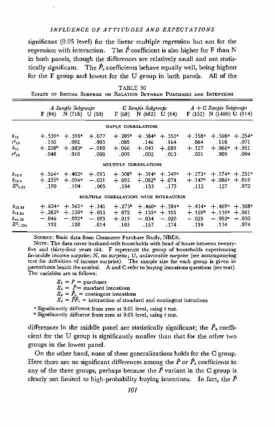
Table 30 summarizes correlations for husband-wife households withthe head between twenty-five and thirty-four years of age. The toppanel shows simple correlation and regression coefficients for the A and Csamples and for the two samples combined. The middle panel hascoefficients for a multiple regression in which P and P are assumed to belinearly related to P. Results of a multiple regression that allows forinteraction between P and P0 (along the lines discussed in Chapter 5) aresummarized in the bottom panel.

The data in Table 30 are rather encouraging, considering the hodge-podge of coefficients in the regression analysis described earlier. Thelinear multiple regressions are apt to be the most reliable, since the inter-action term in the bottom panel tends to make the regression coefficientsquite sensitive to sampling variations; because of the way in which surpriseis defined, both the favorably surprised group (F) and the unfavorablysurprised group (U) are quite small. The A sample shows results thatare almost wholly in accord with the proposition that P is less closelyassociated with P for those with unfavorable surprises than for either ofthe other two groups, and that PC is more closely associated with P forthose with favorable surprises than for either of the other groups. Thenet regression coefficient of P in the two lower panels is substantially lowerfor the U group than for either of the other two groups; the differences are

150


significant (0.05 level) for the linear multiple regression but not for theregression with interaction. The P coefficient is also higher for F than Nin both panels, though the differences are relatively small and not statis-tically significant. The P> coefficients behave equally well, being highestfor the F group and lowest for the U group in both panels. All of the

TABLE 30EFFECT OF INCOME SURPRISE ON RELATION BETWEEN PURCHASES AND INTENTIONS

A Sa

F (84)mple Subgroups C Sample Subgroups

N (718) U (50) F (68) N (682) U (64)A + C

F (152)Sample Subgroups

N (1400) U (114)

SIMPLE CORRELATIONS

b12

r2ss

b1,

2is

+.539a.130

+228'>.048

+396> +077 +.289b +.384> +.353a.092 .003 .085 .146 .164

+083> —.010 +.066 +043 +.089.010 .000 .009 .002 .013

+.358a.084

+127.021

+368> +.254>.118 .071

+066> +.051.005 .004

MULTIPLE CORRELATIONS

b,2,,

b,3.5

R21.2,

+564>+255'>

.190

+.402a +093 +308'> +394> +.349a+094> — .031 +095 +.082' +074

.104 .005 .104 .153 .173

+373>+.147b

.112

+,374a +251>+086> +019

.127 .072

MULTIPLE CORRELATIONS WITH INTERACTION

b11.,4

b,3.24

b142,

R11.234

+634>+282'>—.046

.192

+561> +341 +.273' +.460> +.384>+150> +055 +.072 +.135> +.105— .092> — .093 +.019 — .034 — .020

.120 .014 .105 .157 .174

+414>+169'>— .025

.114

+469> +308>+139> +061— .052> — .030

.134 .074

SOURCE: Basic data from Consumer Purchase Study, NBER.NOTE: The data cover husband-wife households with head of house between twenty-

five and thirty-four years old. F represents the group of households experiencingfavorable income surprise; N, no surprise; U, unfavorable surprise (see accompanyingtext for definition of income surprise). The sample size for each group is given inparentheses beside the symbol. A and C refer to buying intentions questions (see text).The variables are as follows:

Xs = P = purchases

= P = standard intentions= = contingent intentions= PP = interaction of standard and contingent intentions

Significantly different from zero at 0.01 level, using t test.b Significantly different from zero at 0.05 level, using t test.

differences in the middle panel are statistically significant; the P coeffi-cient for the U group is significantly smaller than that for the other twogroups in the lowest panel.

On the other hand, none of these generalizations holds for the C group.Here there are no significant differences among the P or P2 coefficients inany of the three groups, perhaps because the P variant in the C group isclearly not limited to high-probability buying intentions. In fact, the P

161


variable for group C is not very different from the algebraic sum of P andPC in group A, judging from data in Chapter 2.

When the two groups are combined, the pattern shown by the A groupis somewhat diluted but still clearly apparent. The reliability of thecombined results is greater because the sample sizes for the F and U groupsare about twice as large as before; but the reliability is presumably reducedby the difference in the meaning of standard and contingent intentionsin the two groups. In the bottom panel the U group;has a lower P coef-ficient than either F or N, and the P coefficient is not significantly differentfor F and N. The F group has the highest P coefficient; the U group,the lowest.

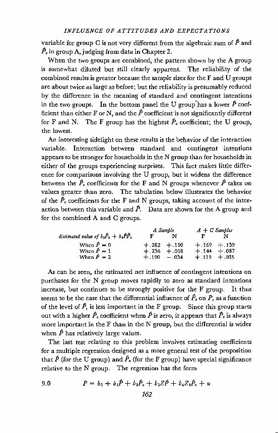
An interesting sidelight on these results is the behavior of the interactionvariable. Interaction between standard and contingent intentionsappears to be stronger for households in the N group than for households ineither of the groups experiencing surprises. This fact makes little differ-ence for comparisons involving the U group, but it widens the differencebetween the A coefficients for the F and N groups whenever P takes onvalues greater than zero. The tabulation below illustrates the behaviorof the P coefficients for the F and N groups, taking account of the inter-action between this variable and P. Data are shown for the A group andfor the combined A and C groups.

A Sample A + C SamplesEstimated value of b,P + b4PP F N F N

WhenP=0 +282 +.150 +.169 +.139When P = 1 +.236 +.058 +.144 +.087When P = 2 +.190 —.034 +119 +.035

As can be seen, the estimated net influence of contingent intentions onpurchases for the N group moves rapidly to zero as standard intentionsincrease, but continues to be strongly positive for the F group. It thusseems to be the case that the differential influence of P, on F, as a functionof the level of P, is less important in the F group. Since this group startsout with a higher P coefficient when P is zero, it appears that PC is alwaysmore important in the F than in the N group, but the differential is widerwhen P has relatively large values.

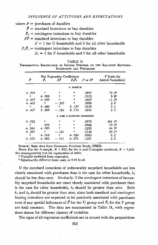
The last test relating to this problem involves estimating coefficientsfor a multiple regression designed as a more general test of the propositionthat P (for the U group) and P (for the F group) have special significancerelative to the N group. The regression has the form

9.0 P=bo+b1P+b2P0+b3ZP+b4Z1P+u162

iNFLUENCE OF ATTITUDES AND EXPECTATIONS

where P purchases of durablesP standard intentions to buy durablesA, contingent intentions to buy durables

zP standard intentions to buy durablesZ = 1 for U households and 0 for all other householdscontingent intentions to buy durables

= 1 for F households and 0 for all other households

TABLE 31DIFFERENTIAL IMPORTANCE OF INCOME SURPRISE ON THE RELATION BETWEEN

INTENTIONS AND PURCHASES

PNet ReP

gression CoefficientsZP Z1P, r2 or R2

F Ratio forAdded Variable(s)

A SAMPLE

+394

+.397+405

+407

a

+088+095

a

+080+089

a a .0887a a .0103a a .1007

— .245 a .0908a +.137 .0139

—.186 +.116 .1056

754b8.8b

1l.2b

2.0

3.1

2.3A AND C SAMPLES COMBINED

+.312a

+364+.367

a

+.373

.070

+085a

+068+085

a a .0970a a .0062a a .1210

— .121 a .1128a +.024 .0063

— .111 +.071 .1231

161.4b

lO.3b443b

29.1"

0.2

2.0

SOURCE: Basic data from Consumer Purchase Study, NBER.NOTE: For the A sample, N = 852; for the A and C samples combined, N = 1,666.

See accompanying text for explanation of table.a Variable excluded from regression.b Significantly different from unity at 0.01 level.

If the standard intentions of unfavorably surprised households are lessclosely associated with purchases than is the case for other households, b3'should be less than zero. Similarly, if the contingent intentions of favora-bly surprised households are more closely associated with purchases thanis the case for other households, b4 should be greater than zero. Bothb1 and b2 should be greater than zero, since both standard and contingentbuying intentions are expected to be positively associated with purchaseseven if any special influences of P for the U group and P5 for the F groupare held constant. The data are summarized in Table 31, with regres-sions shown for different clusters of variables.

The signs of all regression coefficients are in accord with the propositions163


advanced above, although the Z and Z1 terms generally do not make astatistically significant contribution to explained variance. The mostappropriate test of the two interaction variables consists of comparingthe results for the last equation in each panel with those for the third.The difference between these two equations is that both interactionvariables have been added to a regression including P and P; in neitherpanel does the combined influence of the additional variables add sig-nificantly to the explanation of purchases. On the other hand, ZP makesa significant contribution to the explanation of P in the lower panel(compare the first and fourth equations), and some of the other variablesinvolving Z or are significant at the 0.10 level, though not at 0.05.17

Tests similar to those summarized in Table 31 were run on differentsubgroups with results that were not as consistent. In other subsamplesone of the interactions generaLly had the expected sign while the otherbehaved erratically. For example, in the subsample composed ofhusband-wife households with the head between thirty-five and forty-fouryears old, the U group had a smaller coefficient for standard intentionsthan either the F or N group, as predicted. But this same group alsohad a larger coefficient for contingent intentions than either the F or Ngroup, which makes no particular sense. The contingent-plan coefficientfor F was in turn higher than that for N, in accordance with expectations.None of the differences in regression coefficients were large enough to bestatistically significant.

Summary

The results of this investigation into the relation among durable goodspurchases, buying intentions, expectations, and/or surprises can best becategorized as suggestive of possible relationships but inconclusive as towhether expectations and/or surprises are actually related to purchasesnet of buying intentions. A nonlinear relation between expectations andpurchases seems quite probable, because extremely optimistic (pessimistic)expectations are associated with relatively high (low) purchases, whilemoderate optimism (pessimism) appears to be unrelated to purchases.Whether this relation continues to exist net of buying intentions has notbeen examined above, but evidence to be presented later suggests that

17 These interaction terms do not show significance partly because each is relevantfor only a small proportion of the total cases and, hence, each makes a relatively smallcontribution to total explained variance for all cases taken together. This seems to bethe reason why the ZP term in the top panel increases explained variance by a triflingamount (compare the first and fourth equations) despite its very large absolute size.The ZP term is relevant in only 50 (of 852) cases. Although these cases fit considerablybetter when ZP is included along with P, the remaining cases are affected only veryslightly. The net improvement is not statistically significant.

164


some net relation between a nonlinear index of expectations and pur-chases may well be present. Still, even the best fit obtained (betweenpurchases and a cubic equation involving expectations) was able toexplain less than 1 per cent of the variance in purchases. This perform-ance stands in sharp contrast to the 10 to 20 per cent of the variance inpurchases typically explained by intentions to buy.

Similarly, I was unable to find any simple relation between surprisesand purchases net of buying intentions. Experiments with a morestringent definition of favorable and unfavorable surprise suggested thepossibility that favorable surprises, in interaction with contingent buyingintentions, may be positively related to purchases; unfavorable surprises ininteraction with standard buying intentions may be negatively related topurchases. The evidence in support of these propositions is a long wayfrom being convincing. While the data generally yield regression coeffi-cients with the appropriate signs, many of the coefficients are not sig-nificantly different from zero; the contribution to explained variance isgenerally very small; and in some cases, the data yield coefficients withinappropriate signs. Still, the results are sufficiently promising to suggestthat these relations are worth further investigation and are potentiallyvaluable in explaining consumer behavior.

Finally, the results in this chapter suggest that only rather large devia-tions from average experience are of much value in explaining the relationof expectations and/or surprises to purchase behavior. In effect, theseresults seem to indicate that households with very optimistic expectationsor very favorable surprises are likely to buy considerably more durablegoods, other things being equal; those with very pessimistic expectations orvery unfavorable surprises, considerably fewer. These extreme cases areof little quantitative importance to the sort of data I have been using.The vast bulk of households in a cross section do not fall into either ofthese categories, and the evidence suggests that the necessarily modestdifferences in expectations or surprises among households in the middlegroup are not related to differences in behavior. But it does not followthat these variables play an equally minor role in the explanation ofdifferences in purchase behavior over time. Although only a small(absolute) number of households experience either extreme expectationsor surprises during any one period, the time series variance in the numberof such households is likely to be considerable. This fact, coupled withthe possibility of a quantitatively important association between extremeexpectations or surprises and purchases, may mean that an importantpart of the time series variation in purchases is associated with changes inthe proportion or number of households in these extreme categories.

7ö5

the influence of attitudes and expectations on purchases · to purchase consumer durable...

Documents