The Incidence of Local Labor Demand Shocks

Matthew J. Notowidigdo∗

University of Chicago Booth School of Business and NBER

First Version: November 2009This Version: March 2013

Abstract

Low-skill workers are comparatively immobile: when labor demand slumps in a city,low-skill workers are disproportionately likely to remain to face declining wages and employ-ment. This paper estimates the extent to which (falling) housing prices and (rising) socialtransfers can account for this fact using a spatial equilibrium model. Nonlinear reducedform estimates of the model using U.S. Census data document that positive labor demandshocks increase population more than negative shocks reduce population, this asymmetryis larger for low-skill workers, and such an asymmetry is absent for wages, housing values,and rental prices. GMM estimates of the full model suggest that the comparative immo-bility of low-skill workers is not due to higher mobility costs per se, but rather a lowerincidence of adverse labor demand shocks.

Keywords: local labor markets, mobility costs, durable housing supply, social trans-fers.

JEL Classification: J01, R31, H53.

∗This is a revised version of the first chapter of my dissertation. I am grateful to Daron Acemoglu, David Autor,and Amy Finkelstein for their guidance and support. I also thank Leila Agha, Josh Angrist, Fernando Duarte,Tal Gross, Erik Hurst, Cynthia Kinnan, Jean-Paul L’Huillier, Amanda Pallais, Jim Poterba, Michael Powell,Nirupama Rao, Bill Wheaton, and seminar participants at MIT, Northwestern, Berkeley, Harvard KennedySchool, University of Chicago, Wharton, Stanford, Yale School of Management, Brown, and the 2011 SEDAnnual Meeting for helpful comments. I gratefully acknowledge the National Institute of Aging (NIA grantnumber T32-AG000186) and the MIT Shultz Fund for financial support.

1 Introduction

When a city experiences an adverse labor demand shock, the share of the adult population with

a college degree tends to decline (Glaeser and Gyourko, 2005). A standard explanation for this

pattern is that barriers to mobility are greater for low-skill workers (Topel, 1986; Bound and

Holzer, 2000).1

This paper proposes and tests an alternative explanation which focuses on why low-skill

workers may be disproportionately compensated during adverse labor demand shocks, rather

than why it may be disproportionately costly for them to out-migrate. This explanation has

two components. First, as documented below, adverse shocks substantially reduce the cost of

housing. This fact and the existing evidence that the expenditure share on housing declines

with income imply that low-skill workers are disproportionately compensated by housing price

declines.2 Second, means-tested public assistance programs disproportionately compensate low-

skill workers during adverse shocks. I document below that, not surprisingly, aggregate transfer

program expenditures are highly responsive to local labor market conditions.

These two different types of explanations —one based on mobility costs and one based on

compensating factors — are not incompatible; however, their relative importance ultimately

determines the actual incidence of local labor demand shocks. If out-migration of workers is

low primarily because of mobility costs, then the incidence of local labor demand shocks will be

primarily borne by workers; additionally, to the extent that mobility costs are greater for low-skill

workers, they may disproportionately bear the incidence of the adverse shock. Alternatively, if

the incidence of adverse local labor demand shocks is primarily borne by immobile housing and

social insurance programs, then low-skill workers will be disproportionately compensated and,

1The existence of greater barriers to mobility for low-skill workers is consistent with a large empirical literaturethat has documented that the local labor supply elasticity is larger for high-skill workers than for low-skill workers.For example, Bound and Holzer (2000) find that the elasticity of local labor supply with respect to wages issignificantly higher for college-educated workers than for workers with no more than a high school education.Similarly, Topel (1986) finds that local labor demand shifts generate much smaller wage differentials among moreeducated workers. Topel writes “consistent with the greater geographic mobility of more educated workers, theirwages are less sensitive to both current and future changes in relative employment.”

2Of course, if low-skill workers are homeowners and not renters, then there is a negative wealth effect inaddition to the decline in the user cost of housing following a negative local labor demand shock. Consistentwith much of the recent urban economics literature (e.g., Glaeser and Gyourko (2005) and Moretti (2009)), Iassume in the model below that everyone is a renter. I also explore alternative specifications which assume thatthe demand for housing is homothetic, so that the expenditure share on housing is assumed to be the same forhigh-skill and low-skill workers.

1

consequently, less likely to out-migrate.

In this paper, I develop and estimate a spatial equilibrium model which captures how wages,

population, housing prices, and transfer payments re-equilibrate following a shift in local labor

demand. The model is based on the spatial equilibrium model in Roback (1982). Following

Glaeser and Gyourko (2005), the model in this paper allows for a concave local housing supply

curve, arising from the durability of the local housing stock.3 While the Glaeser and Gyourko

model assumes perfect mobility, I allow for heterogeneous mobility costs which limit spatial

arbitrage, as in Topel (1986). Unlike the preceding models, I explicitly model local labor

demand.

To give the basic intuition of the model, consider the following simplified version.4 The main

conceptual experiment in the model is that a single city experiences a (positive or negative)

labor demand shock while a large number of other cities remain unchanged. Figures 1 and 2

provide graphical representations of the different equilibrium responses of wages, population and

housing prices for four scenarios, depending on whether housing supply is constant elasticity or

asymmetric and whether workers are perfectly mobile or face mobility costs when out-migrating.

Figure 1 depicts the equilibrium response when the elasticity of supply of housing is constant.5

The figure shows a positive shift in the labor demand curve which raises wages by ∆. This

increase in wages causes in-migration, which bids up housing prices until the increase in housing

costs exactly offsets the wage increase (thus restoring the equilibrium no-arbitrage condition for

workers). If workers are perfectly mobile, then the figure shows that the effect of a negative shock

(−∆) is symmetric; i.e., wages, housing prices, and population adjust by equal and opposite

magnitudes (as shown by LA− in the figure). This symmetry comes from the log-linearity of the

housing supply curve and the perfect mobility of workers. If, alternatively, workers face non-

negligible mobility costs, then there will be less out-migration following a negative shock. With

3Throughout the paper I use the term “concave housing supply curve”to imply that positive housing demandshocks increase housing prices less than equal-sized negative shocks reduce housing prices. More formally, aconcave housing supply curve implies that ∂2(housing price)/∂(housing supply)2 < 0.

4In this simplified version of the model, workers in a city inelastically supply labor so that net migration fullydetermines local labor supply. Workers also do not differ in productivity, and there are no transfer payments.The full model below introduces high-skill and low-skill workers as well as transfer payments. Firms are perfectlymobile so that labor demand is perfectly elastic. Homogeneous housing units are supplied by absentee landlordswho live in other cities, and workers consume a fixed expenditure share of housing (sh).

5This is equivalent to assuming that the housing supply curve is log-linear.

2

non-negligible mobility costs, the no-arbitrage condition is now that the marginal worker must be

indifferent between staying and paying c to out-migrate. In this case, both the population and

housing price responses are asymmetric: positive shocks increase population and housing prices

more than negative shocks reduce them (see LB− in the figure). Intuitively, while mobility costs

constrain out-migration, they do not similarly constrain in-migration because there are a large

number of potential in-migrants with negligible mobility costs (since the single city is assumed

to be small relative to the rest of the world). Therefore, the increase in population following

a positive shock is the same whether or not workers face heterogeneous costs of out-migration

(see L+− in the figure)

In Figure 2, the housing supply elasticity is no longer constant. Specifically, housing is more

elastically supplied following an increase in housing demand than a decrease in demand. As

discussed in greater detail in the main text below and in Online Appendix Section A.2, this

asymmetric housing supply curve is consistent with a simple model of durable housing where

housing units are not destroyed once created (Glaeser and Gyourko, 2005). When workers are

perfectly mobile, housing prices respond symmetrically (despite the asymmetry in the housing

supply curve). Intuitively, housing costs still must adjust to exactly offset the wage changes.

Only population responds asymmetrically (as shown by LC− in the figure). However, if workers

have heterogeneous mobility costs to out-migrate as described above, then in this case the

asymmetry of the population response is even greater (see LD− in the figure), and housing prices

also respond asymmetrically.

These scenarios give the intuition for the following two implications of the full model derived

below: (1) if positive labor demand shocks increase population more than negative shocks reduce

population, this suggests the existence of a concave housing supply curve and/or heterogeneous

mobility costs, and (2) if positive shocks increase housing prices more than negative shocks

reduce housing prices, that is consistent with the existence of heterogeneous mobility costs. The

full model below shows that these implications continue to hold in a richer setting with transfer

payments and two types of workers.

The model guides the empirical strategy, which consists of two steps. In the first step, I test

for asymmetric responses of wages, employment, population, and housing prices to symmetric

labor demand shocks. The validity of this exercise requires constructing plausibly exogenous

3

positive and negative shifts in local labor demand of equal magnitude. This paper follows Bar-

tik (1991) in constructing an instrumental variable for local labor demand shocks by interacting

cross-sectional differences in industrial composition with national changes in industry employ-

ment shares. I find robust evidence using U.S. Census data that positive local labor demand

shocks increase population (and employment) more than negative shocks reduce population (and

employment) and that this asymmetry is greater for low-skill workers. These robust asymmet-

ric relationships for local population and employment contrast sharply with the absence of any

evidence of a similar asymmetric relationship for (any measure of) wages, housing values, and

rental prices, though all of these other variables respond strongly to local labor demand.6 As the

spatial equilibrium model makes clear, these results are consistent with a concave local housing

supply curve and limited mobility costs. While the Bartik (1991) procedure has been widely

used in labor economics and urban economics, to my knowledge this is the first paper which uses

this procedure to explicitly test for asymmetric responses of wages, employment, and population

to local labor demand shocks.

To quantitatively estimate the magnitude of mobility costs by skill and the shape of the

housing supply curve, in the second step of the empirical analysis, I estimate the full spatial

equilibrium model using a nonlinear, simultaneous equations GMM estimator. The GMM es-

timates suggest that the housing supply curve is concave and that mobility costs (defined as

a fraction of income) are at most modest and are comparable for both high-skill and low-skill

workers. The GMM results reveal several other important findings. First, the observed asym-

metric population responses are primarily accounted for by an asymmetric housing supply curve

rather than due to substantial barriers to mobility. Second, the results suggest that the ob-

served difference in out-migration by skill is primarily accounted for by transfer payments rather

6The model in Glaeser and Gyourko (2005) predicts a concave relationship between housing prices and theexogenous labor demand, and these authors find supportive evidence of this prediction using an exogenousshock based on climate. As discussed in more detail in the Online Appendix Section A.4, the key differencebetween the model in this paper and the model in Glaeser and Gyourko (2005) is that the model in this paperassumes that housing units are homogeneous, while in the Glaeser and Gyourko model housing units haveheterogeneous, location-specific amenities. In other words, in the Glaeser and Gyourko model, exogenous shocksinduce compositional changes in the distribution of location-specific amenities in the housing stock, and thesecompositional changes affect the (unconditional) average housing price. The difference in empirical results comesfrom the fact that Glaeser and Gyourko (2005) use mean temperature to construct local amenity shocks basedon a dummy variable for whether or not the January mean temperature is greater than 29.1 degrees whereas Iuse variation in local labor demand.

4

than to differences by skill in housing expenditure shares. Third, the results suggest that the

primary explanation for the comparative immobility of low-skill workers is not higher mobility

costs per se, but rather a lower incidence of adverse local labor demand shocks. Consequently,

much of the incidence of adverse labor demand shocks is diffused to homeowners, landlords, and

public assistance programs.

Finally, I use the GMM estimates to construct counterfactual estimates of how local labor

markets would adjust to shocks if the system of means-tested transfer payments was replaced

with a system of mobility subsidies for both high-skill and low-skill workers. In this alternative

system, the skill composition of the local labor force is much less responsive to shifts in local labor

demand, but population continues to respond strongly asymmetrically due to the asymmetric

housing supply curve. The estimation of the full model necessarily requires stronger assumptions

than were needed to test for asymmetric responses to shocks. In order to be able to consistently

estimate the relative magnitude of mobility costs by skill, I must assume that unobserved changes

in local amenities induced by local labor demand shocks are not differentially valued by high-

skill and low-skill workers. To be able to consistently estimate the absolute magnitude of

mobility costs, however, a stronger assumption is needed; namely, that unobserved changes in

local amenities are uncorrelated with local labor demand shocks. Because of this, the analysis

of the absolute magnitudes of mobility costs should be interpreted more cautiously.

This paper is broadly related to recent empirical work which acknolwedges the importance of

migration costs in determining spatial equilibrium. This work has emphasized the importance

of imperfect mobility in determining the effi ciency of place-based policies (Busso, Gregory, and

Kline 2012) and in determining the marginal willingness to pay for environmental amenities

(Bayer, Keohane, and Timmins 2008). This paper is also related to recent work on the effects of

wage income and welfare income on the individual migration decision (Kennan and Walker 2010,

2011); this paper is highly complementary to these two papers, which employ a very different

empirical approach by estimating a rich structural model of individual migration decisions.7

The rest of the paper proceeds as follows. Section 2 presents the theoretical framework.

Section 3 discusses the empirical strategy and the data. Section 4 presents the reduced form

7Also related to this paper is the recent literature on the causal effect of education and geographic mobility(Wozniak, 2006; Malamud and Wozniak, 2008).

5

empirical results. Section 5 investigates the robustness of these results. Section 6 presents

GMM estimates of the full model. Section 7 concludes.

2 Theoretical Framework

This section presents a simple spatial equilibrium model of a local labor market that captures

how wages, population, housing prices, and transfer payments re-equilibrate following a local

labor demand shock.8 The heart of the model is a no-arbitrage condition in which the marginal

worker is indifferent between remaining in the city receiving the shock and moving away (Roback,

1982). This condition implicitly defines a local labor supply curve which determines the amount

of migration in response to a labor demand shock. The model below allows for mobility costs,

which limit spatial arbitrage and cause the incidence of the labor demand shock to fall at least

partially on workers (Topel, 1986).9 Additionally, the model admits two types of workers

(high-skill and low-skill) who differ in productivity, imperfectly substitute in production, and

may potentially differ in their housing expenditure shares, eligibility for transfer payments, and

mobility costs. If an adverse labor demand shock causes relatively greater out-migration of

high-skill labor, the model clarifies when this is because the incidence of the shock is borne

by other factors that disproportionately compensate low-skill workers and when this is due to

greater barriers to mobility for low-skill workers.

The conceptual experiment is that a single city (out of a large universe of cities) experiences a

labor demand shock between the first and second period. For simplicity, the model is presented

as a two-period model in order to rule out the effects of long-run expectations, the differences

between temporary and permanent shocks, the option value from moving, and other issues

arising in dynamic spatial equilibrium models. I focus on decadal changes in the empirical

analyses below in order to minimize the influence of these other factors, and I leave a rigorous

treatment of these dynamics for future work.

To give the general intuition of the model, consider an adverse local labor demand shock in

8The model is a “local general equilibrium”model in the sense that labor demand shocks affect non-labormarkets within the city; however, it is not a full general equilibrium model because when the single city isshocked, the (minimal) effects on the rest of the universe are ignored.

9Topel (1986) is primarily concerned with understanding differences between permanent and transitory shocks;in the simple two-period model in this paper, all shocks are necessarily permanent.

6

a city. This shock will reduce wages, which encourages out-migration and, ultimately, lowers

housing prices until the no-arbitrage condition is restored for the marginal worker. The amount

of out-migration is determined by the magnitude of mobility costs, the generosity of transfer

payments, and the elasticity of supply of housing in response to a decline in housing demand.

The four main components of the model (labor demand, transfer payments, housing market,

and labor supply) are now discussed in detail.

2.1 Labor Demand

Assume a large number of cities indexed by i, and define the (large) number of high-skill and

low-skill workers in city i and time t as Hit and Lit. Production of the homogeneous tradable

good y is given by the following CES aggregate production function:10

yit = θit((1− λ)Lρit + λ(ζHit)ρ)α/ρ

where λ is a share parameter, α measures the returns to scale of the labor aggregate, ζ is the

relative effi ciency of high-skill labor and ρ is related to the elasticity of substitution between

high-skill and low-skill labor by σH,L ≡ 1/(1− ρ).11 The θit term is a city-specific index of local

labor demand. In the empirical section below, I argue that my instrumental variable for local

labor demand is a plausibly exogenous source of variation in θit.

Assuming wages are set on the demand curve, then they are given by the following marginal

productivity conditions:

wHit = αθit((1− λ)Lρit + λ(ζHit)ρ)(α−ρ)/ρλζ(ζHit)

ρ−1

wLit = αθit((1− λ)Lρit + λ(ζHit)ρ)(α−ρ)/ρ(1− λ)(Lit)

ρ−1

Totally differentiating the above wage expressions results in the following conditions for

the evolution of wages in terms of exogenous labor demand shock (∆θit) and the endogenous

10For simplicity, capital is not included in the model. This could be important if part of the incidence of labordemand shocks falls on owners of capital. Since the empirical results are based on decadal changes, it seemsreasonable to assume that the elasticity of supply of capital over this time period is fairly large.11Let µ be the share of high-skill workers in the labor market. Then if λ = (1−µ)ρ−1/((ζµ)ρ−1 + (1−µ)ρ−1),

ζ will give the equilibrium wage premium.

7

migration responses (∆Hit and ∆Lit):

∆wHit = ∆θit + ((ρ− 1) + (α− ρ)(π)) ∆Hit + (α− ρ)(1− π)∆Lit (1)

∆wLit = ∆θit + ((ρ− 1) + (α− ρ)(1− π)) ∆Lit + (α− ρ)(π)∆Hit (2)

where π = λ(ζH)ρ/((1− λ)Lρ + λ(ζH)ρ), and the ∆ operator represents the percentage change

over time.

2.2 Transfer Payments

Means-tested public assistance programs are available only to low-skill workers and are modeled

as a constant elasticity function of wages:12

bit = B · (wLit)Ψ

where bit is the transfer income (social assistance benefits) for the representative low-skill worker,

B is a constant, andΨ is the elasticity of public assistance income with respect to low-skill wages.

The constant elasticity assumption is a simplification; empirically, I do not find robust evidence

of a nonlinear or asymmetric effect of labor demand shocks on aggregate expenditures on transfer

programs, so this assumption appears to be a reasonable approximation. The equations above

imply the following expression for the evolution of transfer income in response to changes in

low-skill wages:

∆bit = Ψ∆wLit (3)

I assume Ψ < 0, which implies that transfer programs provide wage insurance, and I define sLb

as the share of total income that comes from transfer program benefits for low-skill workers; for

high-skill workers, sHb = 0.

12Using PSID data from 1990, I calculate that 0.5% of households receiving AFDC income during the pastyear had a household head with at least a college degree. Among households receiving food stamps during thepast year, the fraction is 0.7%. By contrast, among households receiving AFDC income, 79.1% had a householdhead with a high school education or less; for food stamps, the fraction is 82.6%. Therefore, means-tested publicassistance program benefits are primarily used by households with low-skill household heads.

8

2.3 Housing Market

A homogeneous housing stock is supplied by absentee landlords, and the aggregate housing

supply curve is given by HS(pHit ), where pHit is the price of housing. Workers have identical

preferences over housing and the homogeneous tradable consumption good. Existing empiri-

cal estimates suggest that housing consumption is a normal good with an income elasticity of

demand less than one; for example, Polinsky and Ellwood (1979), find a (permanent) income

elasticity of 0.80 − 0.87. These results imply that the demand for housing is non-homothetic

and suggest that the expenditure share of housing should be lower for high-skill workers. Using

data from the Consumer Expenditure Survey, this is evident in the cross-section: in 1995, the

housing expenditure share declines by more than 8 percentage points going from bottom 20% in

income to top 20% in income distribution, declining from 38.5% to 30.0%.13 Defining sHH and

sLH as the housing expenditure shares for high-skill and low-skill workers, respectively, then these

facts indicate that sLH > sHH. In the GMM estimates below, I report results assuming sLH > sHH

and results which assume sLH = sHH.

Insetad of assuming a specific utility function to derive the demand for housing, I instead

approximate aggregate demand for housing as follows

HD(pHit ) =sHHw

HitHit + sLH(bLit + wLit)Lit

pHit

This expression is an approximation since I am implicitly assuming that any changes in income

induced by a shift in labor demand are small so that income effects can be ignored. Empirically,

the changes in wages within skill groups are small relative to the differences in wages across skill

groups, so this assumption is sensible.

The initial supply-demand equilibrium in housing market in the first period is given by

HS(pHit ) = HD(pHit ). Totally differentiating this equilibrium condition gives the following ex-

pression for the housing market response:

∆pHit + ∆HS(∆pHit ) = ν(∆yHit + ∆Hit) + (1− ν)(∆yLit + ∆Lit) (4)

13Expenditure share by quintile (going from lowest to highest income quintile) is the following: 38.5%, 32.9%,31.8%, 30.0%, and 30.0%.

9

where ν is the high-skill share of aggregate housing demand and ∆yjit gives the change in total

income for skill group j (∈ {H,L}); i.e., ∆yjit = sjb∆bjit+(1−sjb)∆w

jit. If the housing supply curve

has constant elasticity, then ∆HS(pHit ) = σ · ∆pHit . Since housing is a durable good, however,

the housing supply elasticity is not likely to be constant. Instead, the housing supply elasticity

will be larger for increases in housing demand than for decreases in housing demand due to

the durability of the housing stock (Glaeser and Gyourko, 2005). Formally, durable housing

implies that ∆HS(∆pHit ) is increasing in ∆pHit . The Online Appendix Section A.4 presents a

simple model which provides microfoundations for a concave housing supply curve based on slow

depreciation of the housing stock and a heterogeneous distribution of costs of supplying housing.

2.4 Labor Supply

For simplicity, I assume that workers inelastically supply labor to their local labor market, so

that all variation in local employment comes only from migration decisions. The local labor

supply curve is then implicitly defined by a mobility condition which states that the marginal

migrant must be indifferent between remaining in city i and moving to any other city.

I introduce costly spatial arbitrage by assuming that workers have heterogeneous mobility

costs. I construe mobility costs broadly to encompass both financial and psychic barriers to

out-migration as well as heterogeneous tastes and distastes for a given location. Thus unlike

Topel (1986), I allow mobility costs to take on positive and negative values. Positive values

encompass both actual moving costs as well as preferences for the current city, while negative

values represent distaste of potential in-migrants for a given area. Formally, I model this by

assuming that mobility costs for workers in city i are independently drawn from distributions

MHi (m) and ML

i (m) (with support [0,∞)), while the mobility costs of in-migrating into city

i for the workers living in all of the other cities are drawn from the distributions MH−i(m) and

ML−i(m) (with support (−∞, 0]). Mobility costs are defined as a fraction of total income, so

that the marginal migrant receiving (w + b) in city i will pay (w + b)m to out-migrate. These

mobility cost distributions imply mobility cost functions cH(∆Hit) and cL(∆Lit), which return

the mobility cost of the marginal migrant given the change in population between the first and

second period. For a smooth distribution of mobility costs, the mobility cost function will be

10

strictly decreasing, so that the mobility cost of the marginal migrant increases as more workers

out-migrate.14

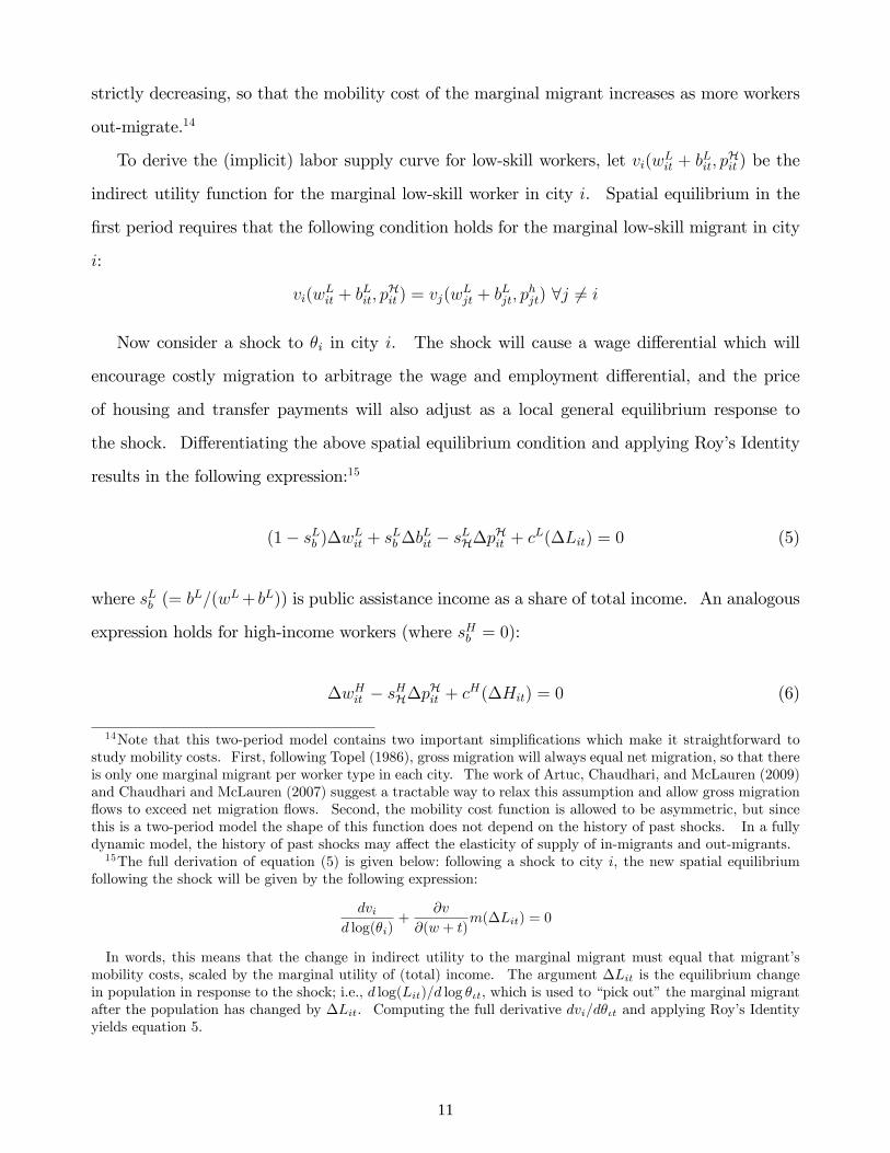
To derive the (implicit) labor supply curve for low-skill workers, let vi(wLit + bLit, pHit ) be the

indirect utility function for the marginal low-skill worker in city i. Spatial equilibrium in the

first period requires that the following condition holds for the marginal low-skill migrant in city

i:

vi(wLit + bLit, p

Hit ) = vj(w

Ljt + bLjt, p

hjt) ∀j 6= i

Now consider a shock to θi in city i. The shock will cause a wage differential which will

encourage costly migration to arbitrage the wage and employment differential, and the price

of housing and transfer payments will also adjust as a local general equilibrium response to

the shock. Differentiating the above spatial equilibrium condition and applying Roy’s Identity

results in the following expression:15

(1− sLb )∆wLit + sLb ∆bLit − sLH∆pHit + cL(∆Lit) = 0 (5)

where sLb (= bL/(wL+ bL)) is public assistance income as a share of total income. An analogous

expression holds for high-income workers (where sHb = 0):

∆wHit − sHH∆pHit + cH(∆Hit) = 0 (6)

14Note that this two-period model contains two important simplifications which make it straightforward tostudy mobility costs. First, following Topel (1986), gross migration will always equal net migration, so that thereis only one marginal migrant per worker type in each city. The work of Artuc, Chaudhari, and McLauren (2009)and Chaudhari and McLauren (2007) suggest a tractable way to relax this assumption and allow gross migrationflows to exceed net migration flows. Second, the mobility cost function is allowed to be asymmetric, but sincethis is a two-period model the shape of this function does not depend on the history of past shocks. In a fullydynamic model, the history of past shocks may affect the elasticity of supply of in-migrants and out-migrants.15The full derivation of equation (5) is given below: following a shock to city i, the new spatial equilibrium

following the shock will be given by the following expression:

dvid log(θi)

+∂v

∂(w + t)m(∆Lit) = 0

In words, this means that the change in indirect utility to the marginal migrant must equal that migrant’smobility costs, scaled by the marginal utility of (total) income. The argument ∆Lit is the equilibrium changein population in response to the shock; i.e., d log(Lit)/d log θιt, which is used to “pick out”the marginal migrantafter the population has changed by ∆Lit. Computing the full derivative dvi/dθιt and applying Roy’s Identityyields equation 5.

11

Equations (5) and (6) are implicit labor supply curves because net migration is determined

by the spatial equilibrium condition for the marginal migrant. In words, the conditions above

state that the change in indirect utility in response to changes in wages, transfer payments, and

housing prices must equal the mobility costs of the marginal migrants. The ∆Lit and ∆Hit

terms represent the amount of net migration that needs to occur to make these two equations

hold.

These two equations highlight the three reasons discussed in the introduction why net mi-

gration rates may differ by skill. First, public assistance program benefits are means-tested, so

that sLb > sHb . Second, low-skill workers consume a larger fraction of their income on housing

sLH > sHH, meaning that housing price declines disproportionately compensate low-skill workers.

Finally, the mobility cost functions may differ by skill. If low-skill workers typically face higher

mobility costs following a negative shock, then cL(x) > cH(x) ∀x < 0.

2.5 Equilibrium

Following an exogenous shock to local labor demand (∆θit), the new equilibrium of the model

is defined by the following conditions:

• Labor demand adjusts so that high-skill and low-skill wages equal marginal products (equa-

tions (1) and (2)).

• Transfer payments adjust according to changes in low-skill wages (equation (3)).

• Housing prices adjust so that the change in housing demand equals the change in housing

supply (equation (4)).

• Population adjusts so that the marginal high-skill and low-skill migrant is indifferent be-

tween staying and leaving (equations (5) and (6)).

Although the nonlinearities in the housing supply curve (∆HS(∆pHit )) and the mobility cost

functions (cH(∆Hit) and cL(∆Lit)) preclude analytical solutions without particular functional

form assumptions, Section A.2 in the Online Appendix derives comparative statics for specific

scenarios under the special case of constant returns to scale of production (α = 1).

12

Figure 3 reports results from simulating the model.16 The figure shows that if population

responds asymmetrically, it suggests the existence of a concave housing supply curve and/or

the existence of heterogeneous mobility costs. The responsiveness of housing prices isolates the

importance of heterogeneous mobility costs, since mobility costs cause immobile workers to bid

up the price of housing during negative shocks, causing housing prices to respond asymmetrically.

Therefore, the model suggests that it is possible to identify both mobility costs and the shape

of the housing supply curve by using information on the joint responses of wages, population,

housing prices, and transfer payments to exogenous labor demand shocks.

These simulations motivate the two-part empirical strategy below. First, I will estimate

nonlinear reduced form regressions to test for asymmetric responses to labor demand shocks.

Second, I will carry out a full estimation of the model to recover the parameters which govern

the distribution of mobility costs and the shape of the housing supply curve.

3 Empirical Strategy and Data

As the model makes clear, the reduced form relationships between each of the endogenous

variables (∆wH , ∆wL, ∆H, ∆L, ∆ph, ∆tL) and the labor demand shock ∆θ are informative

about the shape of housing supply curve and the presence of heterogeneous mobility costs. This

motivates the following reduced form estimating equation:

∆xit = gx(∆θit) + αt + ∆εit

where i indexes cities, t indexes time periods, x is one of the endogenous variables above, αt

captures proportional shocks to all cities in a given time period, εit is an error term, and g() is

a function to be estimated. Nonparametric estimates of g() are reported graphically below. In

addition to the nonparametric estimates, I also parameterize gx(∆θ) as β(∆θ) + δ(∆θ)2 which

leads to the following baseline reduced form empirical specification that is reported in the tables:

∆xit = β ×∆θit + δ × (∆θit)2 + αt + εit (7)

16The details of the simulation are given in Section A.3 in the Online Appendix.

13

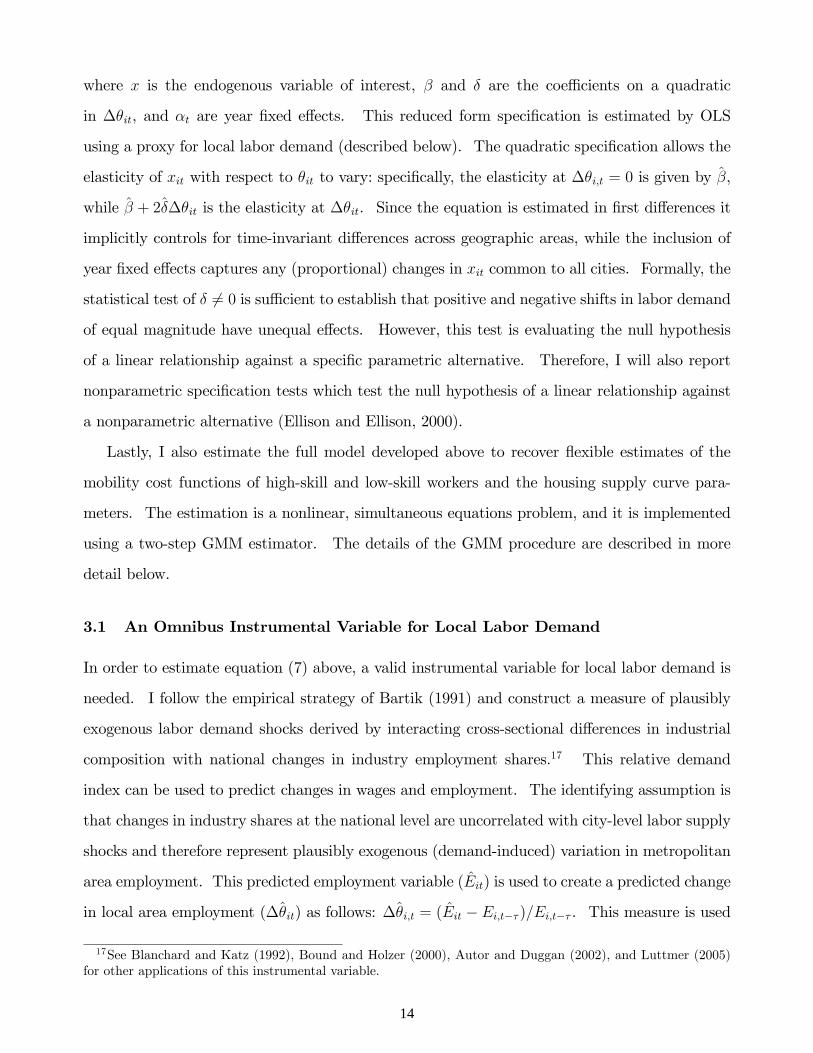
where x is the endogenous variable of interest, β and δ are the coeffi cients on a quadratic

in ∆θit, and αt are year fixed effects. This reduced form specification is estimated by OLS

using a proxy for local labor demand (described below). The quadratic specification allows the

elasticity of xit with respect to θit to vary: specifically, the elasticity at ∆θi,t = 0 is given by β,

while β + 2δ∆θit is the elasticity at ∆θit. Since the equation is estimated in first differences it

implicitly controls for time-invariant differences across geographic areas, while the inclusion of

year fixed effects captures any (proportional) changes in xit common to all cities. Formally, the

statistical test of δ 6= 0 is suffi cient to establish that positive and negative shifts in labor demand

of equal magnitude have unequal effects. However, this test is evaluating the null hypothesis

of a linear relationship against a specific parametric alternative. Therefore, I will also report

nonparametric specification tests which test the null hypothesis of a linear relationship against

a nonparametric alternative (Ellison and Ellison, 2000).

Lastly, I also estimate the full model developed above to recover flexible estimates of the

mobility cost functions of high-skill and low-skill workers and the housing supply curve para-

meters. The estimation is a nonlinear, simultaneous equations problem, and it is implemented

using a two-step GMM estimator. The details of the GMM procedure are described in more

detail below.

3.1 An Omnibus Instrumental Variable for Local Labor Demand

In order to estimate equation (7) above, a valid instrumental variable for local labor demand is

needed. I follow the empirical strategy of Bartik (1991) and construct a measure of plausibly

exogenous labor demand shocks derived by interacting cross-sectional differences in industrial

composition with national changes in industry employment shares.17 This relative demand

index can be used to predict changes in wages and employment. The identifying assumption is

that changes in industry shares at the national level are uncorrelated with city-level labor supply

shocks and therefore represent plausibly exogenous (demand-induced) variation in metropolitan

area employment. This predicted employment variable (Eit) is used to create a predicted change

in local area employment (∆θit) as follows: ∆θi,t = (Eit − Ei,t−τ )/Ei,t−τ . This measure is used

17See Blanchard and Katz (1992), Bound and Holzer (2000), Autor and Duggan (2002), and Luttmer (2005)for other applications of this instrumental variable.

14

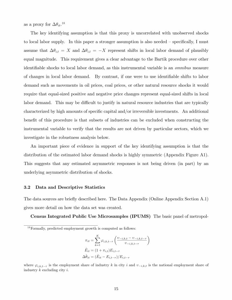
as a proxy for ∆θit.18

The key identifying assumption is that this proxy is uncorrelated with unobserved shocks

to local labor supply. In this paper a stronger assumption is also needed —specifically, I must

assume that ∆θi,t = X and ∆θi,t = −X represent shifts in local labor demand of plausibly

equal magnitude. This requirement gives a clear advantage to the Bartik procedure over other

identifiable shocks to local labor demand, as this instrumental variable is an omnibus measure

of changes in local labor demand. By contrast, if one were to use identifiable shifts to labor

demand such as movements in oil prices, coal prices, or other natural resource shocks it would

require that equal-sized positive and negative price changes represent equal-sized shifts in local

labor demand. This may be diffi cult to justify in natural resource industries that are typically

characterized by high amounts of specific capital and/or irreversible investments. An additional

benefit of this procedure is that subsets of industries can be excluded when constructing the

instrumental variable to verify that the results are not driven by particular sectors, which we

investigate in the robustness analysis below.

An important piece of evidence in support of the key identifying assumption is that the

distribution of the estimated labor demand shocks is highly symmetric (Appendix Figure A1).

This suggests that any estimated asymmetric responses is not being driven (in part) by an

underlying asymmetric distribution of shocks.

3.2 Data and Descriptive Statistics

The data sources are briefly described here. The Data Appendix (Online Appendix Section A.1)

gives more detail on how the data set was created.

Census Integrated Public Use Microsamples (IPUMS) The basic panel of metropol-

18Formally, predicted employment growth is computed as follows:

πit =K∑k=1

ϕi,k,t−τ

(υ−i,k,t − υ−i,k,t−τ

υ−i,k,t−τ

)Eit = (1 + πi,t)Ei,t−τ

∆θit = (Eit − Ei,t−τ )/Ei,t−τ

where ϕi,k,t−τ is the employment share of industry k in city i and υ−i,k,t is the national employment share ofindustry k excluding city i.

15

itan area data comes from the 1980, 1990, and 2000 Census individual-level and household-level

extracts from the IPUMS database (Ruggles et al., 2004).19 The baseline data are limited to

individuals and households living in metropolitan areas. The IPUMS data are used to construct

estimates of local area wages, employment, population, housing prices, and rental prices in each

metropolitan area. The primary advantage of the Census data is the ability to construct city-

level measures disaggregated by skill. These data are also used to construct the predicted labor

demand instrumental variable by using the industry categories of the individuals in the labor

force. See the Data Appendix for remaining details.

Regional Economic Information System (REIS) The metropolitan-area measures

of expenditures on public assistance programs are computed by aggregating the county-level

aggregate data in the REIS. The REIS contains annual county-level data on total expenditures

broken down by transfer program (e.g., food stamps, income maintenance programs, public

medical benefits, veterans benefits, SSI benefits). Counties are aggregated into metropolitan

areas using the 1990 Metropolitan Statistical Area (MSA) definitions. Because of the diffi culty

in aggregating counties into MSAs within Alaska and Virginia during this time period, MSAs

in these states are dropped from the baseline sample. Though the data are not disaggregated

below the county-level, the data are based on government agency reports and are therefore quite

reliable. According to recent work by Meyer, Mok, and Sullivan (2009), aggregate expenditure

data may be sometimes preferable to individual or household survey data due to substantial

underreporting in the latter.20 All transfer program measures are adjusted per low-skill capita

based on the non-college adult population.

Table 1 reports descriptive statistics for the final data set.

19The 2007 American Community Survey (ACS) is included as a robustness check. The 1970 Census is notused at all because it identifies only a small subset of the MSAs that appear in later years.20Meyer, Mok, and Sullivan (2009) find substantial underreporting of benefit receipt in a wide range of data sets,

including the CPS, PSID, SIPP, and the Consumer Expenditure Survey for a wide range of transfer programs.They also document that the under-reporting is not consistent over time.

16

4 Results

4.1 Graphical Evidence

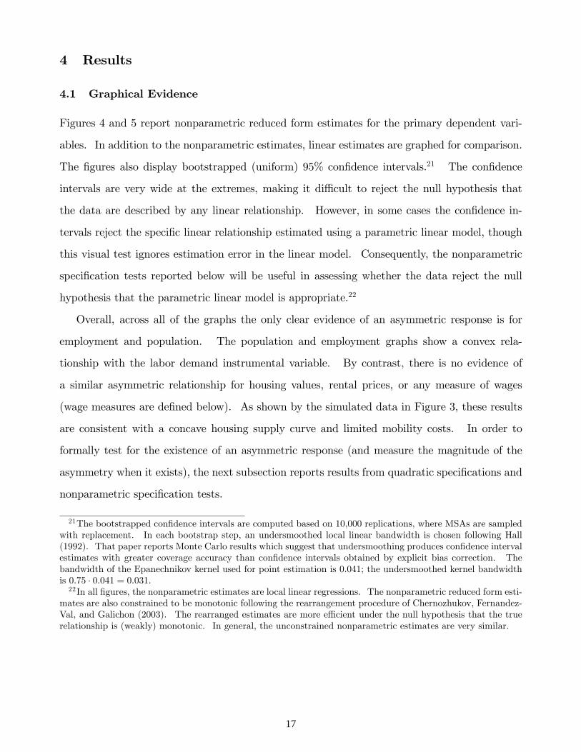
Figures 4 and 5 report nonparametric reduced form estimates for the primary dependent vari-

ables. In addition to the nonparametric estimates, linear estimates are graphed for comparison.

The figures also display bootstrapped (uniform) 95% confidence intervals.21 The confidence

intervals are very wide at the extremes, making it diffi cult to reject the null hypothesis that

the data are described by any linear relationship. However, in some cases the confidence in-

tervals reject the specific linear relationship estimated using a parametric linear model, though

this visual test ignores estimation error in the linear model. Consequently, the nonparametric

specification tests reported below will be useful in assessing whether the data reject the null

hypothesis that the parametric linear model is appropriate.22

Overall, across all of the graphs the only clear evidence of an asymmetric response is for

employment and population. The population and employment graphs show a convex rela-

tionship with the labor demand instrumental variable. By contrast, there is no evidence of

a similar asymmetric relationship for housing values, rental prices, or any measure of wages

(wage measures are defined below). As shown by the simulated data in Figure 3, these results

are consistent with a concave housing supply curve and limited mobility costs. In order to

formally test for the existence of an asymmetric response (and measure the magnitude of the

asymmetry when it exists), the next subsection reports results from quadratic specifications and

nonparametric specification tests.

21The bootstrapped confidence intervals are computed based on 10,000 replications, where MSAs are sampledwith replacement. In each bootstrap step, an undersmoothed local linear bandwidth is chosen following Hall(1992). That paper reports Monte Carlo results which suggest that undersmoothing produces confidence intervalestimates with greater coverage accuracy than confidence intervals obtained by explicit bias correction. Thebandwidth of the Epanechnikov kernel used for point estimation is 0.041; the undersmoothed kernel bandwidthis 0.75 · 0.041 = 0.031.22In all figures, the nonparametric estimates are local linear regressions. The nonparametric reduced form esti-

mates are also constrained to be monotonic following the rearrangement procedure of Chernozhukov, Fernandez-Val, and Galichon (2003). The rearranged estimates are more effi cient under the null hypothesis that the truerelationship is (weakly) monotonic. In general, the unconstrained nonparametric estimates are very similar.

17

4.2 Reduced Form Results

This section reports estimates of equation (7) above to investigate the responsiveness of wages,

employment, and population to changes in local labor demand. The baseline reduced form

estimating equation is reproduced below:

∆xit = β ×∆θit + δ × (∆θit)2 + αt + ∆εi,t

The baseline results are reported in Tables 2 through 4. Table 2 presents results for overall

population, employment, and wages. Column (1) shows the results for the total population

between the ages of 18 and 64.23 The estimate of β is precise and strongly statistically sig-

nificant (p < 0.001), which verifies that the measure of predicted employment changes strongly

predicts actual shifts in local population. The estimate of δ is also economically and statisti-

cally significant (δ = 28.010, s.e. 7.905). One way to interpret the magnitude of this estimate

is to calculate the marginal effect at one standard deviation greater than zero and one standard

deviation less than zero; these estimates are −0.152 and 3.757, respectively, and the difference

between these estimates is strongly statistically significant (p < 0.001).24 Additionally, a non-

parametric specification test strongly rejects the null hypothesis that the relationship is linear

in favor of a nonparametric alternative (p < 0.001).25 In other words, the results in this column

suggest that positive changes in local labor demand increase population more than negative

changes reduce population. The results for employment in column (2) show evidence of a sim-

ilar convex relationship. The results in column (3) using the percentage point change in the

employment-to-population ratio show that not all of the reduction in local employment from an

adverse shock comes from net out-migration; there is also a decline in labor force participation.

23Results using the population between the ages of 25 and 54 are very similar.24Note that the p-value for the test of whether the marginal effects are the same at one standard deviation

above and below zero is exactly the same as the p-value for the test of whether the quadratic term is statisticallysignificantly different from zero.25I use the nonparametric specification test procedure suggested by Ellison and Ellison (2000), which groups

the data into “bins”and creates a test statistic that is asymptotically distributed as a standard normal randomvariable. To my knowledge, there is a not a data-driven procedure to select the proper bin width; therefore, I viewthe nonparametric specification test as complementary to the quadratic specification. While the nonparametricspecification test does not rely on a specific parametric alternative, it is not possible to ensure that I have theright size and power in constructing my statistical tests. In almost all of the results that follow, inference basedon the quadratic specification and the nonparametric specification test is similar.

18

The remaining columns of Table 2 explore the consequences of local labor demand shifts

on wages. There are (at least) two diffi culties in constructing an appropriate wage measure.

The first diffi culty is that the labor demand shock may induce compositional changes in the

population, so that the change in the average wage will be confounded by composition effects.

The second diffi culty is that changes in labor force participation reduce income per adult, but

would be excluded using a measure of average wages based only on employed workers.

I approach these problems by first presenting two measures of changes in wage income which

should represent upper and lower bounds of the true change in income holding characteristics

of the workers fixed. The first measure (following Bound and Holzer (2000)) is the total wage

income per 18-64 adult. This measure will account for demand-induced changes in labor force

participation but will also include compositional changes. The results are in column (4) and

show a large effect of local labor demand on wages (β = 0.959, s.e. 0.137). The second measure

(following Shapiro (2003) and Albouy (2009a, 2009b)) uses the individual-level census data

and regresses log wages of employed workers on a large set of controls and MSA fixed effects

(see Data Appendix for details). The MSA fixed effect estimated from this regression is a

composition-adjusted measure of the wage premium which I define as the “residualized wage”.26

The results in column (5) using this measure show a much smaller wage response (β = 0.353, s.e.

0.086). However, this second measure does not account for changes in labor force participation.

Assuming that at least some of the observed change in labor force participation is involuntary,

then this measure will understate the total effect of the demand shock. To address this concern,

I take the residualized wage measure and multiply it by the observed labor force participation

rate.27 I call this the “adjusted wage”and use this as the preferred wage measure. This measure

accounts for both compositional changes in the labor force in response to the shock as well as

changes in labor force participation, and therefore essentially assumes that reservation wages

are negligible. Consequently, I expect this measure to provide an overestimate of mobility costs

when I ultimately estimate the full model via GMM. As a way of bounding the estimated

26This measure is similar to the local wage premiums calculated in Shapiro (2003) and Albouy (2009a, 2009b).This measure does not control for unobservable changes in the composition of labor force. If unobservablechanges in composition of labor force move in the same direction as observable changes, then the measuredresponse of wages will be upward biased, and estimates of mobility costs will be conservative.27Note that when I present results by skill below, I use the labor force participation rate in the given skill

group to adjust the residualized wage measure.

19

magnitude of mobility costs, I also report GMM estimates which use the residualized wage

instead of the adjusted wage. The residualized wage will give a lower bound on the estimated

magnitude of mobility costs, as it assumes reservation wages are approximately equal to accepted

wages for all employed workers.

As expected, the magnitude of the effect of local labor demand for adjusted wages lies in

between the other two wage measures (β = 0.520, s.e. 0.109). Since the magnitude of changes in

labor force participation is modest, the estimates for adjusted wages are closer to the estimates

for residualized wages than the estimates using the per capita income measure. Regardless of

the measure of wages used, however, the important conclusion that emerges from columns (4)

through (6) is that there is no evidence of an asymmetric response of wages to shifts in local

labor demand in any of the wage measures. It is only population and local employment which

respond asymmetrically.

Table 3 reports results on population, employment and wages separately for high-skill and

low-skill workers. I define low-skill workers as those without a college degree, and high-skill

workers as those with at least a college degree. The patterns in Table 2 are reproduced when

looking separately within each skill group: population and employment respond asymmetrically,

and there is no evidence of a similar asymmetric response for either high-skill or low-skill wages.

Furthermore, the magnitude of the wage effects are similar across high-skill and low-skill workers,

consistent with the assumption that the labor demand shifts are factor-neutral.28 Additionally,

columns (5) and (6) show suggestive evidence that the skill composition of the adult population

and labor force also responds asymmetrically. In other words, negative shocks reduce college

share of adult population more than positive shocks increase college share. I emphasize that

this asymmetric response is not as robust as the estimated asymmetric responses for population

and employment for each skill group. As the simulations in Figure 3 makes clear, when an

asymmetric population responses arises from either a concave housing supply curve or hetero-

geneous costs of out-migration, there is (at most) a small asymmetric responses in the high-skill

population share.

Next, Table 4 looks at three important non-labor outcomes: real estate rental prices, housing

28Results from stacked regressions do not reject the null hypothesis that the average wage response for high-skillworkers is the same as the average wage response for low-skill workers (p = 0.523).

20

values, and aggregate expenditures on public assistance programs. The measures of average

rental prices and housing values are purged of observable changes in the quality of the housing

stock following a similar procedure to the one used to create the residualized wage measure

(see Data Appendix for details). Column (1) in Table 4 reports results for rental prices, which

respond strongly to local labor demand. The results for housing values in column (2) are similar

in magnitude, though somewhat less precise. As with the wage results, there is no evidence

of an asymmetric response in either column; the estimates of δ are statistically insignificant

and at most modest in magnitude, and the nonparametric specification tests fail to reject the

parametric (linear) model in both columns.29 Appendix Table A2 reports similar results using

the unconditional average rental prices and average housing values, as well as results using the

repeated-sales housing price index (HPI) published by the Federal Housing Finance Agency

(FHFA), formerly the Offi ce of Federal Housing Enterprise Oversight (OFHEO). Consistent

with the results in Table 4, there is no evidence of an asymmetric response in any of these

alternative specifications.

Lastly, column (3) reports estimates using aggregate expenditures on Food Stamps and

Income Maintenance Programs. The results show that expenditures on these programs respond

strongly to local labor market conditions. The estimated magnitude of the response is large (β =

−2.367) and implies that a 1% decline in local labor demand increases aggregate expenditures on

these two programs by 2.4%. Though the quadratic term is marginally significant (p = 0.074),

the nonparametric test does not reject the linear model (p = 0.241), suggesting that the nonlinear

relationship estimated in the quadratic specification is not robust.30

A setting in which population and employment respond asymmetrically to positive and neg-

ative labor demand shocks while wages, rental prices, and housing values respond symmetrically

is consistent with the model simulation where mobility costs are limited and the housing supply

curve is concave. Before moving beyond this qualitative conclusion to quantitative estimates

of mobility costs and housing supply curve parameters, I next document that these reduced

29Additionally, results from stacked regressions reject that the quadratic terms are the same for populationand rental prices (p = 0.0004) and reject that the quadratic terms are the same for population and housing values(p = 0.001).30Appendix Table A3 reports estimates for various other transfer programs, including Medicare, Disability

Benefits, SSI, and Veterans Benefits, and the results are qualitatively similar. I focus on Food Stamps andIncome Maintenance income because these programs are explicitly designed to smooth consumption.

21

form results are not driven by unobserved trends, outliers, sample selection, or heterogeneous

industry-specific effects. After that, I conclude by estimating the full model above using a

nonlinear GMM estimator.

5 Robustness

5.1 Industry Trends

The main results in Table 2 emphasize the importance of asymmetric employment and popula-

tion responses to local labor demand shocks, and the absence of a similar asymmetric response

for wages, housing prices, and transfer payments. The key identifying assumption in interpreting

these results is that equally-sized positive and negative predicted changes in local employment

represent shifts in local labor demand of plausibly equal magnitude. Because the predicted

changes are formed by interacting cross-sectional variation in industrial composition with na-

tional changes in industry shares, an obvious concern is that qualitatively different industries are

declining and expanding. If these industries would not be expected to have otherwise identical

responses to shifts in local labor demand (perhaps because of differences in relative demand for

high-skill labor, the amount of specific human capital in the industry, or the ability of firms in

the industry to respond and adjust to shocks), then this would cast doubt on the interpretation

of the results as tracing out an asymmetric local labor supply curve.

To investigate this concern, I categorize industries based on their decadal changes in total

national employment. Industries are grouped into one of four categories:

1. Persistently expanding/declining industries. Industries where employment either increased

in every decade or decreased in every decade.

2. Stable industries. Industries where employment did not increase or decrease more than

20% in any of the decades.31

3. Volatile industries. Industries that experienced employment growth of more than 20%

and decreases of more than 20% during the sample period.

31If industries are classified as both persistently expanding/declining and stable, I categorize the industry asstable. This definition and the cutoff of 20% were chosen to give roughly equal-sized categories. Results aresimilar with nearby cutoffs.

22

4. Other industries. Industries not otherwise categorized.

The top twenty industries according to average national employment share in each of these

categories are listed in Appendix Table A1. The industries in each of the categories conform to

expectations given the secular industry trends during this time period. Persistently expanding

industries are concentrated in services, health care, data processing, and leisure goods, while per-

sistently contracting industries are in apparel, publishing, manufacturing, and tobacco. Volatile

industries include natural resource industries such as oil and gas extraction as well as defense

industries. I begin by constructing predicted employment excluding variation in national em-

ployment shares for industries that are persistently expanding or persistently declining.32 The

resulting relative demand index is purged of any variation caused by secular trends in health

care, services, and manufacturing. Table 5 reports results from estimating equation (7) using

this alternative measure of predicted employment as an instrumental variable for local labor de-

mand. Panel A reports results with the change in adult population as the dependent variable.

Column (1) reproduces the results from column (1) in Table 2 for comparison. Column (2)

reports results using the predicted employment measure that does not use any variation from

industries which are persistently expanding or persistently declining. The point estimates in

column (2) are fairly similar to the baseline estimates reproduced in column (1). Columns (3)

through (5) report results excluding each of the other industry categories when constructing

predicted employment, and the results are also quite similar to the baseline results in column

(1). The correlation between the labor demand instrument used in columns (2) and (5) is 0.48,

suggesting that the similarity across columns is not simply a mechanical consequence of the

different instruments exploiting similar sources of variation. Moreover, while previous research

has highlighted the high correlation between this labor demand instrument and the share of em-

ployment in manufacturing (Bound and Holzer 2000), the correlation between the instrument in

column (2) and the share of adult population employed in manufacturing is only 0.16. There-

fore, I interpret these results as suggesting that the estimated asymmetric population response

32Formally, predicted employment growth is computed by using only the subset of industries which pass agiven filter:

π′i,t =∑

k∈K′⊂Kϕi,k,t−τ

(υ−i,k,t − υ−i,k,t−τ

υ−i,k,t−τ

)where K is the set of all industries and K ′ is the set of industries which pass the filter.

23

is not primarily due to unobserved, heterogeneous, industry-specific trends or effects.

A related concern is that because of the way that the IPUMS creates consistent industry

codes across time, there are “catch-all” industry codes that collect industries which are not

otherwise categorized. I label an industry code a catch-all industry code if it contains the word

“miscellaneous” or contains the suffi x “not elsewhere categorized.” These catch-all industry

codes make up roughly 10% of the industry codes. These catch-all categories may represent

different collections of industries in different decades, which may bias the main estimates. To

investigate this concern, I create an alternative measure of predicted employment which does

not use any variation in national employment shares of these industries. The estimates using

this predicted employment measure are reported in column (6) and are similar to the results in

column (1), suggesting that there is no significant bias from including these catch-all categories.

Panels B and C of Table 5 report results which repeat this exercise using adjusted wages

and rental prices as the dependent variables, respectively. Consistent with the baseline results

in Tables 2 and 4, none of the estimates in any of the columns show evidence of an asymmetric

relationship between adjusted wages or rental prices and labor demand.33

5.2 Alternative Specifications

I next turn to an investigation of the robustness of the main results by reporting alternative

specifications which vary the sample definition and the set of time-varying controls used. The

purpose of these specifications is primarily to investigate the possibility of sample selection bias

and the potential bias from unobserved trends that are correlated with shifts in local labor

demand. As with Table 5, Table 6 reports results using population, adjusted wages, and rental

prices (respectively) as the dependent variables in each of the panels. All columns report results

from estimating variants of equation (7). In all panels, column (1) reports the baseline results for

comparison. Column (2) reports results from adding data on the 2000-2007 changes.34 Column

(3) creates “pseudo-MSAs”by grouping together all individuals in a state who are not in anMSA.

33Interestingly, the magnitude of the (linear) response of adjusted wages and rental prices to local labor demandvaries somewhat depending on the industries used to generate predicted changes in employment, suggesting thatthe strength of the proxy for local labor demand may vary depending on the set of industries used to generatethe proxy.34The 2000-2007 changes are translated into implied decadal changes by first calculating annual percentage

changes.

24

Column (4) reports long-difference results (using the 1980-2000 change) rather than the stacked

decadal changes as in the baseline specification. Columns (5) and (6) report results including

alternative sets of geographic and time fixed effects. Column (5) includes region fixed effects for

each of the nine census regions which control for region-specific linear time trends, while column

(6) includes controls for MSA-specific linear time trends. Column (7) reports results which test

for the importance of outliers. This column drops the 5% of the data with the largest magnitude

changes in local labor demand. Finally, column (8) uses the County Business Patterns (CBP)

data set to construct the local labor demand instrument rather than using Census data (see

Data Appendix for details). The CBP data contain finer industry categories, which in principle

could reduce measurement error, but there are two primary drawbacks: first, there is a high rate

of suppressed data at the county-by-industry level, and, second, the county-level data must be

aggregated.

Panel A of Table 6 reports results using population as the dependent variable. Across all

of the columns, the point estimates are very similar to the baseline specification in column (1).

The results in column (6) which include MSA-specific linear time trends show a substantial loss

of precision, but the point estimates remain stable. The results in column (7) show that the

estimated asymmetric response is robust to dropping outlying observations, suggesting that the

convex population response is not primarily driven by outliers. The results in column (8) show

the results are similar using CBP data to construct the labor demand instrument.

Panels B and C of Table 6 report results using adjusted wages and rental prices (respectively)

as the dependent variables. The estimates of δ are never statistically significant at conventional

levels, nor are even consistently the same sign across columns. In other words, there is no

consistent evidence of an asymmetric response of adjusted wages or rental prices to local labor

demand shocks.

Lastly, Appendix Table A4 reports specifications which drop each one (of nine) census regions.

This table confirms that the results do not appear to be driven by any particular region.

In summary, the reduced form patterns of a significant asymmetric response of population

and employment to changes in local labor demand appear robust and contrast sharply with a

lack of similar asymmetric responses for wages, housing values, and rental prices.

25

6 GMM Estimates

The reduced form results presented above directly test for the existence of asymmetric responses

of wages, population, employment, and housing prices to symmetric labor demand shocks. While

revealing, these results do not estimate any of the economic parameters in the theoretical model

and are therefore not quantitatively informative about the distribution of mobility costs by skill

and the actual incidence of labor demand shocks. This section reports results from a joint

estimation of the full model using a nonlinear, simultaneous equations GMM estimator. The

econometric setup follows from the theoretical model presented above and imposes moment

conditions which can be used to identify the parameters of interest. In particular, the GMM

estimator can recover flexible estimates of the housing supply curve and mobility cost functions

for high-skill and low-skill workers. These estimates can be used to assess the relative impor-

tance of housing expenditures, transfer payments, and mobility costs in generating the observed

migration patterns in the data. Additionally, because I parameterize the model so that there are

more moment conditions than (remaining) parameters to estimate, the GMM estimator admits

a chi-squared overidentification test of the full model.

To implement the GMM estimator, the following equations (derived from equations (1)

through (6) in the model above) are used:

∆ewHit = ∆wHit − (∆θit + ((ρ− 1) + (α− ρ)(π)) ∆Hit + (α− ρ)(1− π)∆Lit)

∆ewLit = ∆wLit − (∆θit + ((ρ− 1) + (α− ρ)(1− π))∆Lit + (α− ρ)(π)∆Hit)

∆etit = ∆tLit −Ψ∆wLit

∆ehit = ∆pHit + ∆Hs(∆pHit )− (ν(∆wHit + ∆Hit) + (1− ν)((1− sLb )∆wLit + sLb ∆tLit + ∆Lit))

∆eHit = ∆wHit − sHH∆pHit + cH(∆Hit)

∆eLit = (1− sLb )∆wLit + sLb ∆tLit − sLH∆pHit + cL(∆Lit)

where i indexes cities, t indexes time, and ∆ejit represent error terms uncorrelated with shifts

in labor demand.35 These equations jointly solve the local general equilibrium problem of

35Each of these equations can be derived formally by including error terms which proportionally shift pro-duction, housing demand, housing supply, transfer payments, and indirect utility. For example, re-define the

26

how wages, employment, housing prices, and transfer payments respond to an exogenous labor

demand shift ∆θit. The six endogenous variables are the following: ∆pHit , ∆wHit , ∆wLit, ∆Hit,

∆Lit, and ∆bLit. Note that the error terms are allowed to be freely correlated with each other,

which gives rise to simultaneity bias that the GMM estimator is intended to address. The

unknowns in the model are the following parameters and functions:

• Transfer income and housing expenditure shares (sLb , sLH, sHH)

• Aggregate share parameters (µ, ν)

• Labor demand parameters (α, ρ, π, ζ)

• Transfer payment elasticity (Ψ)

• Mobility cost functions (cL(·) and cH(·))

• Housing supply function (∆Hs(·))

In order to reduce the number of parameters to estimate, I first impose values of sLb , sLH,

sHH based on external information. I compute sLb = 0.05 by dividing aggregate expenditures

on Food Stamps and Income Maintenance Programs by the sum of these expenditures and

aggregate low-skill wage income. For the housing expenditure shares, I use sLH = 0.34 for non-

college households and sHH = 0.30 for college-educated households based on the data presented

in Section 2.36

For the labor demand curve, I compute π = 0.37 based on average wages for high-skill and

low-skill workers and average share of high-skill workers in the adult population. I compute

the wage premium (ζ) as 1.75, which is the average wages of college-educated workers divided

by the average wages of non-college workers. I next compute the average share (over this time

period) of college-educated workers in the labor force (µ) as 0.25. Using the formula for π

equilibrium condition for transfer payments as follows: tLit = etit · TL(wLit)ΨL

, where etit is a random variablewhich represents unobservable shocks to transfer payment expenditures (and E[et] = 1). Totally differentiatingthis condition gives the following expression: ∆tLit = ΨL

(∆wLit

)+ ∆etit, which is the equation used in the GMM

estimation.36Average household income is $82,439 for high-skill households in the baseline sample and is $48,456 for

low-skill households. Assuming sHH = 0.30 for high-skill households and income elasticity of 0.8, then sLH = 0.34for low-skill households.

27

in Section 2, this gives π = 0.37. I compute ν = 0.34 based on the average wages, the skill

share, and the housing expenditure shares from above.37 I choose ρ = 0.29 based on Katz and

Murphy (1992).38 This leaves the returns to scale parameter (α) to be estimated. Although

this parameter will be estimated from functional form assumptions, it is still useful to include

the two moments of the labor demand curve to check the overall fit of the model.39 This means

that misspecification in the functional form of labor demand equation will caused bias estimates

in all of the parameters when estimating the entire system of equations. Therefore, I also report

results below which drop the labor demand moments.40

Finally, I choose the following functional forms for the mobility cost functions and housing

supply elasticity:

cj(x) =σj(exp(βjx)− 1)

βjj ∈ {L,H}

∆Hs(x) =σh(exp(βhx)− 1)

βh

These functions are the exponential transformations suggested by Manly (1976), which repre-

sent Box-Cox transformations of exponentiated variables and are defined so that if βj = 0, then

the functions simplify to σjx. These functions are flexible enough to accommodate interesting

curvature with only two parameters, and they are everywhere monotonic and have continuous

first derivatives, which greatly simplifies the computation. Ultimately, there are eight remaining

parameters to estimate {σh, βh, σL, βL, σH , βH , Ψ, α}: two housing supply curve parameters

(σh, βh), two low-skill mobility cost parameters (σL, βL), two high-skill mobility cost parameters

37The aggregate housing demand share parameter is computed using given by ν = µζsHH/(µζsHH + (1− µ)sLH).

38Katz and Murphy (1992) estimate the elasticity of substitution between high-skill and low-skill labor (σH,L)to be 1.4. This gives ρ = 1− 1/σH,L = 0.29.39Since the instrumental variable shifts the labor demand curve, parameters of the labor demand curve itself

are identified from functional form assumptions.40Because the labor demand instrument is measured with error, when using it in the GMM estimation, I

rescale it by regressing adjusted wages on the instrument and scale the instrument so that this regression withthe rescaled instrument would give a coeffi cient of 1.0. A more rigorous alternative is to modify the labordemand moments to include an additional parameter (κ) as follows:

∆ewHit = ∆wHit − (κ∆θit + ((ρ− 1) + (α− ρ)(π)) ∆Hit + (α− ρ)(1− π)∆Lit)

∆ewLit = ∆wLit − (κ∆θit + ((ρ− 1) + (α− ρ)(1− π))∆Lit + (α− ρ)(π)∆Hit)

This procedure yields very similar results.

28

(σH , βH), the responsiveness of transfer payments to low-skill wages (Ψ), and the returns to

scale parameter (α).

The resulting GMM estimator solves a nonlinear, simultaneous equations problem, so in or-

der to estimate the nonlinear parameters I need to take nonlinear functions of the instrumental

variable (∆θ) to achieve identification. I use ∆θ, (∆θ)2, (∆θ)3, (∆θ)4, and (∆θ)5 as instru-

mental variables.41 This results in 30 moment conditions (the five polynomial functions of the

instrument × the six error terms). The full model is estimated using a standard two-step GMM

procedure (see Section A.5 of the Online Appendix for details of this procedure).

The GMM estimates are presented in Table 7. The first row presents the preferred spec-

ification using the external estimates discussed above. Columns (1) and (2) report estimates

of the housing supply curve. The estimates suggest that the housing supply curve is concave

(βh = 6.306, s.e. 1.774). One way to interpret the housing supply coeffi cients is to compute the

increase in housing supply when housing prices exogenously rise by 20% (24.1%) and compare

it to the decrease in housing supply when housing prices decline by 20% (−6.8%). In other

words, the magnitude of housing supply response is about four times larger for an increase in

housing prices than for an equal-sized decrease in housing prices.

The estimates of the mobility cost function parameters (columns (3) through (6)) give no

evidence of an asymmetric mobility cost function for either high-skill or low-skill workers; the

estimates suggest that the mobility cost functions are approximately linear. The point estimates

for σL and σH are precisely estimated and statistically significantly different from zero, suggesting

the existence of non-negligible mobility costs. To get a sense of the magnitudes, the point

estimates imply that the 10th percentile of mobility costs in a city (i.e., the marginal migrant

after 10% of the population has out-migrated following a negative shock) is roughly 17.4% of

annual income for high-skill workers and 17.0% of annual income for low-skill workers.42 In

other words, despite the fact that low-skill workers are disproportionately likely to remain in

41In principle, only the quadratic term is needed ot identify the parameters of the model. Adding additionalpolynomial terms increases statistic power at the cost of introducing bias (either because the orthogonalityassumption is not satisfied at higher moments or the additional polynomial introduces a weak instrumentsproblem). In the absence of a principled procedure to select instruments, I added additional polynomial termsas long as they gave substantial additional statistical precision.42I assume the marginal migrant has 25 years of working life remaining and thus must trade off remaining

to face permanently lower wage and employment opportunities against paying the one-time mobility cost toout-migrate and avoid the adverse wage and employment consequences.

29

declining cities following negative shocks, the point estimates imply that high-skill workers have

very similar mobility costs as a fraction of income (and therefore that low-skill workers have

lower absolute mobility costs on average). Column (7) reports the estimated transfer payment

elasticity, which is quantitatively large and precisely estimated; the coeffi cient implies that a 1%

decline in low-skill wages increases transfer payment expenditures by 3.8% (s.e. 0.5%). Column

(8) reports estimates of the returns to scale parameter (α = 1.038, s.e. 0.025), which suggests

that returns to scale are approximately constant and is consistent with the reduced form results,

which found no evidence of an asymmetric response of wages.43 This is important because

increasing returns to scale are not consistent with the equilibrium conditions of the model. The

p-value in column (8) reports results of testing α = 1; in our baseline model, we are not able

to reject the null of constant returns to scale (p = 0.129). Finally, the results in column (10)

show that the overidentification test does not reject the null hypothesis that the deviations of

the empirical moments from the model are due to chance (p = 0.515).

The remainder of Table 7 reports estimates of the full model under alternative economic

assumptions. The second row reports estimates assuming that both housing expenditure share

and public assistance expenditures do not differ by skill and are negligible (i.e., sHH = sLH = 10−6

and sHb = sLb = 10−6). These estimates verify that ignoring the welfare effects of housing price

adjustments and changes in expenditures on public assistance programs results in much larger

estimates of mobility costs for both high-skill and low-skill workers. In this scenario, the mobility

cost estimates for low-skill workers are significantly larger in magnitude (σL = −0.201 versus

σH = −0.107). Also, the difference between these coeffi cients is highly significant (p < 0.001).

To compare to the baseline estimates, the mobility costs are roughly three times larger for low-

skill workers and two times larger for high-skill workers when ignoring housing costs and transfer

payments.44

The third and fourth rows report model estimates when only housing and only transfers are

“shut down”, respectively. The estimated mobility cost functions from these rows and the first

43Wages did not respond asymmetrically but population and employment did, which suggests constant returnsto scale. If there were decreasing returns to scale, then the asymmetric response of employment to the locallabor demand shock would imply an asymmetric wage response, as well.44The estimated mobility cost functions are also statistically significantly convex, implying that the mobility

cost of the marginal out-migrant rises faster than the marginal in-migrant, although the magnitude of theconvexity is not large.

30

two rows are graphed in Figure 6. Both the figure and the model estimates (see column (9))

suggest that transfer payments are responsible for a majority of the relative difference in mobility

by skill. However, the magnitudes of mobility cost estimates are much larger for both types

of workers when housing expenditures are ignored. In other words, the asymmetric population

response for both high-skill and low-skill workers is primarily due to the asymmetric housing

supply curve, while the differential response by skill is primarily due to transfer payments.

The fifth row assumes the demand for housing is homothetic so that the housing expenditure

shares are the same across the two skill groups. I choose sLH = sHH = 0.33 to match the average

housing expenditure share across the entire population. The results are fairly similar to the

baseline results in the first row, implying that the non-homotheticity assumed in the baseline

model does not substantially account for the differential out-migration rates by skill.

Rows 6 and 7 in Table 7 report estimates which impose alternative values of σH,L. First, I

impose σH,L = 20, which corresponds to the two types of labor being close to perfect substitutes,

and the results are fairly similar. The next row imposes σH,L = 0.1, which corresponds to the

two types being close to perfect complements, and the housing supply curve estimates are much

noisier. Interestingly, the fit of the model is best when using σH,L = 1.4 (row 1) following Katz

and Murphy (1992), as opposed using either of the two extreme values of σH,L.

The next row of Table 7 (row 8) uses an alternative measure of wages. As discussed above,

the preferred measure of wages (“adjusted wages”) assumes that most of the observed change in

labor force participation is involuntary. This measure was chosen to provide an upper bound of

estimated mobility costs. As an alternative, row 7 reports results using the “residualized wage”

measure (see Section 4 for definition). Since residualized wages do not account for changes in

labor force participation, the estimated mobility cost parameters are much lower. In fact, using

this alternative wage measure, I cannot reject the null hypothesis that mobility costs are zero

for low-skill workers. Overall, I conclude that these results suggest that mobility costs for both

high-skill and low-skill workers are at most modest. Even under the extreme assumption that

reservation wages are negligible, the estimated mobility costs are still much lower than would

be implied by focusing solely on wages.45

45The final row reports estimates which drop the labor demand curve moments. The reason why alternativeassumptions on the elasticity of substitution did not substantially affect the estimated mobility cost functions is

31

One use of the GMM estimates is to construct out-of-sample counterfactual simulations of

alternative policies regarding social transfers. Figure 7 reports results from one such simulation.

In this simulation, the system of means-tested transfers (summarized by the parameter Ψ) has

been replaced by a system of mobility subsidies which reduces the mobility costs of all workers

by 50%.46 Each panel in the figure shows the response of a different endogenous variable. The

figure shows that the mobility subsidies increase magnitude of low-skill out-migration following

adverse shocks relative to the system of means-tested transfer payments. Therefore, the high-

skill population share is much less responsive to shifts in local labor demand with mobility

subsidies. One motivation for such a policy would be if there exist strong negative externalities

from increasing the concentration of low-skill workers in a particular area; in this case, mobility

subsidies appear to provide wage insurance to low-skill workers without differentially reducing

their incentive to out-migrate.

7 Conclusion

Low-skill workers are comparatively immobile. When labor demand slumps in a city, college-

educated workers tend to relocate whereas non-college workers are disproportionately likely to

remain to face declining wages and employment. These facts may indicate that mobility is

disproportionately costly for low-skill workers. This paper proposes and tests an alternative

explanation, which is that the incidence of adverse labor demand shocks is borne in large part

by (falling) real estate rental prices and (rising) social transfers. The spatial equilibrium model

developed in this paper illustrates how wages, employment, population, housing prices, and

transfer payments re-equilibrate after a local labor demand shock. Appropriately parameterized,

this model identifies both the magnitude of unobserved mobility costs by skill and the shape of

the local housing supply curve.

Using U.S. Census data, nonlinear reduced form estimates of the effect of plausibly exogenous

that the labor demand moments contribute to identification only indirectly through the optimal GMM weightingmatrix estimated in the first step of the two-step procedure. Therefore, it is not surprising that dropping thelabor demand moments entirely does not significantly affect the estimates of the mobility cost functions (Table7, row 8).46Although this is an obviously stylized form of mobility subsidies, it is not an unrealistic approximation if the

policy took the form of a tax credit that was indexed to income. Recall that mobility costs in the model aredefined as a fraction of annual income.

32

labor demand shocks document that positive labor demand shocks increase population more than

negative shocks reduce population, that this asymmetry is larger for low-skill workers, and that

such an asymmetry is absent for wages, housing values, and rental prices.

These facts are consistent with the presence of limited mobility costs for high-skill and

low-skill workers and a concave housing supply curve (most likely due to a durable housing

stock). Estimates of a full spatial equilibrium model using a nonlinear, simultaneous equations

GMM estimator are consistent with the reduced form evidence and suggest that the primary

explanation for the comparative immobility of low-skilled workers is not higher mobility costs

per se, but rather a lower incidence of adverse local demand shocks.

The finding that mobility costs are limited for both high-skill and low-skill workers is a

necessary condition to be able to properly interpret changes in housing values due to changes

in observed local amenities as a valid marginal willingness to pay for the amenity (see, for

example, Chay and Greenstone (2003)). The results in this paper suggest that the assumption

of perfect mobility may be a valid approximation in some of these hedonic studies, especially

when evaluating changes in local amenities over decadal time horizons. It is worth stressing,

however, that even over decadal time horizons the assumption of perfect mobility is only an

approximation. The preferred GMM estimates in this paper imply non-negligible magnitudes of

mobility costs for both high-skill and low-skill workers following large negative shocks, suggesting

that it may be appropriate to also consider hedonic models which explicitly incorporate barriers

to migration when the underlying changes in local amenities are large, as in Bayer et al. (2008).

One important area of future work is how the incidence of local labor market shocks is

shared between homeowners and renters. On the one hand, homeowners’“user cost”of housing

has declined following a negative labor demand shock; on the other hand, however, declines in

housing values have a negative wealth effect which may affect how responsive the household is to

local labor demand shocks. A full assessment of the incidence of local labor market shocks thus

awaits further study. Another important area of future work is looking at individual transfer

programs. For example, the federal disability insurance program rules suggest that the take-up

decision is generally a once-and-for-all choice, so that disability insurance receipt is an absorbing

state (Autor and Duggan, 2003). The econometric setup in this paper could be used to test

whether positive shifts in local labor demand decrease DI takeup by less than negative shifts

33

increase DI takeup.

Lastly, the finding that mobility costs are limited suggests that transfer payments may be

significantly crowding out the individual migration decision for low-skill workers, which is con-

sistent with the results in the recent “welfare magnetism”literature (see, for example, Gelbach

(2004)). This implies that the social effi ciency of public insurance programs may depend on

the geographic breadth of an adverse labor demand shock, since when a shock is geographically

broad (as during a recession), the gains to relocation are small and there is less scope for transfer

payments to crowd out migration.

34

References

Abraham, Katherine and John C. Haltiwanger. 1995. “Real Wages and the Business Cycle.”Journal of Economic Literature, 33(3): 1215-1264.Albouy, David. 2009a. “The Unequal Geographic Burden of Federal Taxation.” Journal of

Political Economy, 117(4): 635-667.Albouy, David. 2009b. “What are Cities Worth? Land Rents, Local Productivity, and the

Capitalization of Amenity Values.” NBER Working Paper #14981.Artuc, Erhan, Shubham Chaudhuri, and John McLaren. 2010. “Trade Shocks and Labor

Adjustment: A Structural Empirical Approach.” American Economic Review, 100(3): 1008-1045.Autor, David and David Dorn. 2009. “Inequality and Specialization: The Growth of

Low-Skill Service Jobs in the United States,”NBER Working Paper #15150.Autor, David and Mark Duggan. 2006. “The Rise in Disability Rolls and the Decline in

Unemployment.” Quarterly Journal of Economics, 118(1): 157-205.Bayer, Patrick, Nathanial Keohane, and Christopher Timmins. 2008. “Migration and Hedo-

nic Valuation: The Case of Air Quality.” Journal of Environmental Economics and Management,58(1): 1-14.Bartik, Timothy J. 1991. “Who Benefits From State and Local Economic Development

Policies.” W.E. Upjohn Institute for Employment Research: Kalamazoo, Mich.Blanchard, Olivier Jean and Larry Katz. 1992. “Regional Evolutions.” Brookings Papers

on Economic Activity, 1-75.Bound, John and Harry J. Holzer. 2000. “Demand Shifts, Population Adjustments, and

Labor Market Outcomes during the 1980s.” Journal of Labor Economics, 18(1): 20-54.Busso, Matias, Jesse Gregory, and Patrick Kline. 2012. “Assessing the Incidence and

Effi ciency of a Prominent Place Based Policy.” American Economic Review, forthcoming.Chaudhuri, Shubham and John McLaren. 2007. “Some Simple Analytics of Trade and

Labor Mobility.”NBER Working Paper #13464.Chay, Kenneth Y. and Michael Greenstone. 2005.. “Does Air Quality Matter? Evidence

from the Housing Market.” Journal of Political Economy, 113(2): 376-424.Chernozhukov, Victor, Ivan Fernandez-Val and Alfred Galichon. 2009. “Improving Esti-

mators of Monotone Functions by Rearrangement.” Biometrika, 96(3): 559-575.Ellison, Glenn and Sara Fisher Ellison. 2000. “A simple framework for nonparametric

specification testing.”Journal of Econometrics, 96(1): 1-23.Gallin, Josh. 2004. “Net Migration and Labor Market Dynamics.” Journal of Labor

Economics, 22: 1-21.Gelbach, Jonah. 2004. “Migration, the Lifecycle, and State Benefits: How Low is the

Bottom?” Journal of Political Economy. 112(5), 1091-1130.Glaeser, Edward L. and Joseph Gyourko. 2005. “Urban Decline and Durable Housing.”

Journal of Political Economy, 113(2): 345-375.Greene, William H. 2003. Econometric Analysis. Fifth Edition, Prentice Hall: New Jersey.Gould, Eric, David B. Mustard, and Bruce Weinberg. 2002. “Crime Rates and Local Labor

Market Opportunities in the United States: 1979-1997.”Review of Economics and Statistics.84(1): 45-61.Hall, Peter. 1992. “Effect of Bias Estimation on Coverage Accuracy of Bootstrap Confidence

Intervals for a Probability Density.” Annals of Statistics, 20(2): 675-694.

35

Hansen, Lars. 1982. “Large Sample Properties of Generalized Method of Moments Estima-tors.” Econometrica, 50: 1029-1054.Horowitz, Joel. 2001. “The Bootstrap.” Handbook of Econometrics, Volume 5.Hoynes, Hillary. 1999. “The Employment, Earnings, and Income of Less-Skilled Workers

over the Business Cycle.” Institute for Research on Poverty Discussion Paper, no. 1199-99.Jayachandran, Seema. 2006. “Selling Labor Low: Wage Responses to Productivity Shocks

in Developing Countries.” Journal of Political Economy, 114(3): 2006.Katz, Larry and Kevin M. Murphy. 1992. “Changes in Relative Wages, 1963-1987: Supply

and Demand Factors.” Quarterly Journal of Economics, 102(1): 35-78.Kennan, John and James R. Walker. 2011. “The Effect of Expected Income on Individual

Migration Decisions,”Econometrica, 79(1): 211-251.Kennan, John and James R. Walker. 2010. “Wages, Welfare Benefits and Migration,”

Journal of Econometrics, 156(1): 229-238.Luttmer, Erzo. 2005. “Neighbors as Negatives: Relative Earnings and Well-Being.” Quar-

terly Journal of Economics, 120(3): 963-1002.Malamud, Ofer and Abigail Wozniak. 2008. “The Impact of College Graduation on Geo-

graphic Mobility: Identifying Education Using Multiple Components of Vietnam Draft Risk.”NBER Working Paper #16463.Manly, B. F. J. 1976. “Exponential data transformations.” Journal of the Royal Statistical

Society, Series D (The Statistician). 25(1), 37-42.Meyer, Bruce, Wallace K. C. Mok, and James X. Sullivan. 2009. “The Under-Reporting of

Transfers in Household Surveys: Its Nature and Consequences.” Harris School Working Paper#09.03.Morretti, Enrico. 2004. “Estimating the Social Return to Higher Education: Evidence From

Longitudinal and Repeated Cross-Sectional Data.”Journal of Econometrics. 121(1-2).Morretti, Enrico. 2011. “Real Wage Inequality”, mimeo.Polinsky, A. Mitchell and David T. Ellwood. 1979. “An Empirical Reconciliation of Micro

and Macro Grouped Estimates of the Demand for Housing.” The Review of Economics andStatistics, 61(2): 199-205.Roback, Jennifer. 1982. “Wages, Rents, and the Quality of Life.” Journal of Political

Economy, 90(6): 1257-1278.Ruggles, Steven, Matthew Sobek, Trent Alexander, Catherine A. Fitch, Ronald Goeken,

Patricia Kelly Hall, Miriam King, and Chad Ronnander. 2004. Integrated Public Use MicrodataSeries: Version 3.0 [Machine-readable database]. Minneapolis, MN: Minnesota PopulationCenter [producer and distributor].Saiz, Albert. 2010. “The Geographic Determinants of Housing Supply.” Quarterly Journal

of Economics, 125(3): 1253-1296.Saks, Raven. 2005. “Job Creation and Housing Construction: Constraints on Metropolitan

Area Employment Growth.” Finance and Economics Discussion Series 2005-49. Washington:Board of Governors of the Federal Reserve System.Shapiro, Jesse. 2006. “Quality of life, productivity, and the growth effects of human capital.”

Review of Economics and Statistics, 88(2): 324-335.Topel, Robert H. 1986. “Local Labor Markets.” Journal of Political Economy, 94(3):

S111-S143.Wozniak, Abigail. 2010. “Are College Graduates More Responsive to Distant Labor Market

Opportunities?” Journal of Human Resources, 45(4).

36

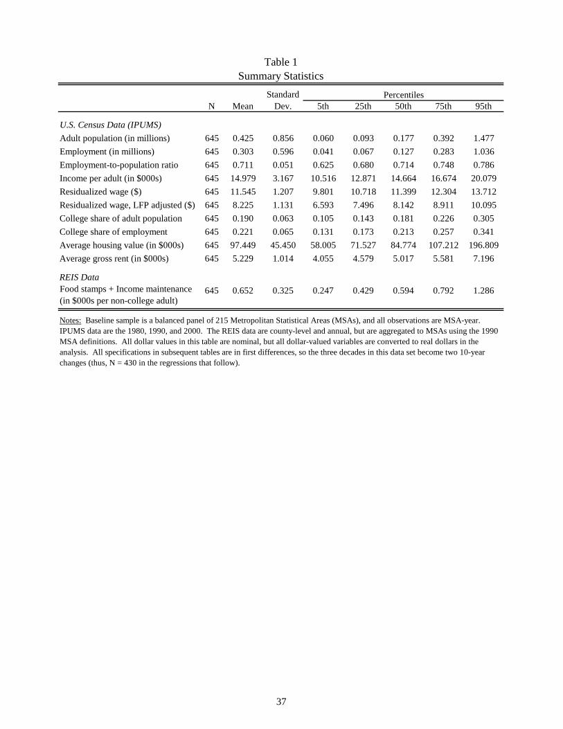
N Mean 5th 25th 50th 75th 95th

U.S. Census Data (IPUMS)Adult population (in millions) 645 0.425 0.856 0.060 0.093 0.177 0.392 1.477Employment (in millions) 645 0.303 0.596 0.041 0.067 0.127 0.283 1.036Employment-to-population ratio 645 0.711 0.051 0.625 0.680 0.714 0.748 0.786Income per adult (in $000s) 645 14.979 3.167 10.516 12.871 14.664 16.674 20.079Residualized wage ($) 645 11.545 1.207 9.801 10.718 11.399 12.304 13.712Residualized wage, LFP adjusted ($) 645 8.225 1.131 6.593 7.496 8.142 8.911 10.095College share of adult population 645 0.190 0.063 0.105 0.143 0.181 0.226 0.305College share of employment 645 0.221 0.065 0.131 0.173 0.213 0.257 0.341Average housing value (in $000s) 645 97.449 45.450 58.005 71.527 84.774 107.212 196.809Average gross rent (in $000s) 645 5.229 1.014 4.055 4.579 5.017 5.581 7.196

REIS Data645 0.652 0.325 0.247 0.429 0.594 0.792 1.286

Table 1Summary Statistics

Notes: Baseline sample is a balanced panel of 215 Metropolitan Statistical Areas (MSAs), and all observations are MSA-year. IPUMS data are the 1980, 1990, and 2000. The REIS data are county-level and annual, but are aggregated to MSAs using the 1990 MSA definitions. All dollar values in this table are nominal, but all dollar-valued variables are converted to real dollars in the analysis. All specifications in subsequent tables are in first differences, so the three decades in this data set become two 10-year changes (thus, N = 430 in the regressions that follow).

StandardDev.

Percentiles

Food stamps + Income maintenance(in $000s per non-college adult)

37

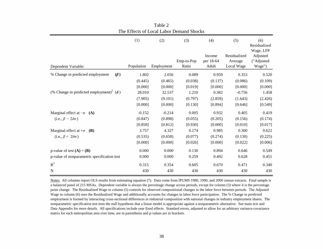
(1) (2) (3) (4) (5) (6)

Dependent Variable: Population EmploymentEmp-to-Pop

Ratio

Income per 18-64

Adult

Residualized Average

Local Wage

Residualized Wage, LFP Adjusted

("Adjusted Wage")

% Change in predicted employment (β ) 1.802 2.056 0.089 0.959 0.353 0.520(0.445) (0.465) (0.038) (0.137) (0.086) (0.109)

[0.000] [0.000] [0.019] [0.000] [0.000] [0.000](% Change in predicted employment)2 (δ ) 28.010 32.537 1.210 0.382 -0.756 1.458

(7.905) (9.101) (0.797) (2.859) (1.643) (2.426) [0.000] [0.000] [0.130] [0.894] [0.646] [0.549]

Marginal effect at −σ (A) -0.152 -0.214 0.005 0.932 0.405 0.419 (i.e., β − 2δσ ) (0.847) (0.898) (0.055) (0.205) (0.156) (0.174)

[0.858] [0.812] [0.930] [0.000] [0.010] [0.017]Marginal effect at +σ (B) 3.757 4.327 0.174 0.985 0.300 0.622 (i.e., β + 2δσ ) (0.535) (0.658) (0.077) (0.274) (0.130) (0.225)

[0.000] [0.000] [0.026] [0.000] [0.022] [0.006]

p-value of test (A) = (B) 0.000 0.000 0.130 0.894 0.646 0.549p-value of nonparametric specification test 0.000 0.000 0.259 0.492 0.628 0.451

R2 0.315 0.354 0.605 0.670 0.471 0.340N 430 430 430 430 430 430

Table 2The Effects of Local Labor Demand Shocks

Notes: All columns report OLS results from estimating equation (7). Data come from IPUMS 1980, 1990, and 2000 census extracts. Final sample is a balanced panel of 215 MSAs. Dependent variable is always the percentage change across periods, except for column (3) where it is the percentage point change. The Residualized Wage in column (5) controls for observed compositional changes in the labor force between periods. The Adjusted Wage in column (6) uses the Residualized Wage and additionally accounts for changes in labor force participation. The % Change in predicted employment is formed by interacting cross-sectional differences in industrial composition with national changes in industry employment shares. The nonparametric specification test tests the null hypothesis that a linear model is appropriate against a nonparametric alternative. See main text and Data Appendix for more details. All specifications include year fixed effects. Standard errors, adjusted to allow for an arbitrary variance-covariance matrix for each metropolitan area over time, are in parenthesis and p-values are in brackets.

38

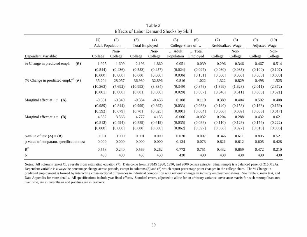
(1) (2) (3) (4) (5) (6) (7) (8) (9) (10)

Dependent Variable: CollegeNon-

College CollegeNon-

College… Adult

Population… Total

Employed CollegeNon-

College CollegeNon-

College

% Change in predicted empl. (β ) 1.925 1.609 2.196 1.860 0.051 0.039 0.296 0.346 0.467 0.514(0.544) (0.436) (0.553) (0.457) (0.024) (0.027) (0.080) (0.085) (0.100) (0.107)

[0.000] [0.000] [0.000] [0.000] [0.036] [0.151] [0.000] [0.000] [0.000] [0.000](% Change in predicted empl.)2 (δ ) 35.204 28.057 36.980 32.896 -0.816 -1.022 -1.322 -0.829 -0.498 1.525

(10.363) (7.692) (10.993) (8.834) (0.349) (0.376) (1.399) (1.628) (2.011) (2.372) [0.001] [0.000] [0.001] [0.000] [0.020] [0.007] [0.346] [0.611] [0.805] [0.521]

Marginal effect at −σ (A) -0.531 -0.349 -0.384 -0.436 0.108 0.110 0.389 0.404 0.502 0.408(0.989) (0.844) (0.999) (0.892) (0.033) (0.038) (0.140) (0.153) (0.168) (0.169)[0.592] [0.679] [0.701] [0.625] [0.001] [0.004] [0.006] [0.009] [0.003] [0.017]

Marginal effect at +σ (B) 4.382 3.566 4.777 4.155 -0.006 -0.032 0.204 0.288 0.432 0.621(0.812) (0.494) (0.889) (0.619) (0.035) (0.038) (0.110) (0.129) (0.176) (0.222)[0.000] [0.000] [0.000] [0.000] [0.862] [0.397] [0.066] [0.027] [0.015] [0.006]

p-value of test (A) = (B) 0.001 0.000 0.001 0.000 0.020 0.007 0.346 0.611 0.805 0.521p-value of nonparam. specification test 0.000 0.000 0.000 0.000 0.134 0.073 0.621 0.612 0.605 0.428

R2 0.558 0.240 0.569 0.262 0.772 0.751 0.432 0.659 0.472 0.210N 430 430 430 430 430 430 430 430 430 430

Table 3Effects of Labor Demand Shocks by Skill

Notes: All columns report OLS results from estimating equation (7). Data come from IPUMS 1980, 1990, and 2000 census extracts. Final sample is a balanced panel of 215 MSAs. Dependent variable is always the percentage change across periods, except in columns (5) and (6) which report percentage point changes in the college share. The % Change in predicted employment is formed by interacting cross-sectional differences in industrial composition with national changes in industry employment shares. See Table 2, main text, and Data Appendix for more details. All specifications include year fixed effects. Standard errors, adjusted to allow for an arbitrary variance-covariance matrix for each metropolitan area over time, are in parenthesis and p-values are in brackets.

Adult Population Total Employed Residualized Wage Adjusted WageCollege Share of …

39

(1) (2) (3)

Dependent Variable:

Residualized Rental Prices

Residualized Housing Values

Food Stamps + Income

Maintenance Expenditures

% Change in predicted employment (β ) 0.842 0.714 -2.367(0.151) (0.360) (0.615)

[0.000] [0.048] [0.000](% Change in predicted employment)2 (δ ) -0.999 -2.765 -21.779

(2.758) (6.310) (12.139) [0.717] [0.662] [0.074]

Marginal effect at −σ (A) 0.912 0.907 -0.847(0.243) (0.580) (1.030)[0.000] [0.119] [0.412]

Marginal effect at +σ (B) 0.773 0.521 -3.887(0.247) (0.558) (1.064)[0.002] [0.351] [0.000]

p-value of test (A) = (B) 0.717 0.662 0.074p-value of nonparametric specification test 0.596 0.295 0.241

R2 0.099 0.144 0.403N 430 430 430

Table 4Effects of Labor Demand Shocks on Housing Market

and Public Assistance Expenditures

Notes: All columns report OLS results from estimating equation (7). Data come from IPUMS 1980, 1990, and 2000 census extracts and the REIS database. The REIS database contains total county-level expenditures on Food Stamps and Income Maintenance programs. These data are aggregated to MSAs using 1990 MSA definition and adjusted per non-college capita using MSA population estimates from the Census. Final sample is a balanced panel of 215 MSAs. Dependent variable is always the percentage change across periods. The % Change in predicted employment is formed by interacting cross-sectional differences in industrial composition with national changes in industry employment shares. See Table 2, main text, and Data Appendix for more details. All specifications include year fixed effects. Standard errors, adjusted to allow for an arbitrary variance-covariance matrix for each metropolitan area over time, are in parenthesis and p-values are in brackets.

40

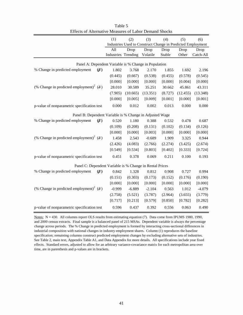
(1) (2) (3) (4) (5) (6)

All Industries

Drop Trending

Drop Volatile

Drop Stable

Drop Other

Drop Catch-All

% Change in predicted employment (β ) 1.802 3.768 2.170 1.855 1.692 2.196(0.445) (0.667) (0.538) (0.455) (0.578) (0.545)

[0.000] [0.000] [0.000] [0.000] [0.004] [0.000](% Change in predicted employment)2 (δ ) 28.010 30.589 35.251 30.662 45.861 43.311

(7.905) (10.665) (13.351) (8.727) (12.455) (13.348) [0.000] [0.005] [0.009] [0.001] [0.000] [0.001]

p-value of nonparametric specification test 0.000 0.012 0.002 0.013 0.000 0.000

% Change in predicted employment (β ) 0.520 1.180 0.388 0.532 0.478 0.687(0.109) (0.208) (0.131) (0.102) (0.134) (0.126)

[0.000] [0.000] [0.003] [0.000] [0.000] [0.000](% Change in predicted employment)2 (δ ) 1.458 2.543 -0.689 1.909 3.325 0.944

(2.426) (4.083) (2.766) (2.274) (3.425) (2.674) [0.549] [0.534] [0.803] [0.402] [0.333] [0.724]

p-value of nonparametric specification test 0.451 0.378 0.069 0.211 0.100 0.193

% Change in predicted employment (β ) 0.842 1.328 0.812 0.908 0.727 0.994(0.151) (0.303) (0.173) (0.152) (0.176) (0.190)

[0.000] [0.000] [0.000] [0.000] [0.000] [0.000](% Change in predicted employment)2 (δ ) -0.999 -6.889 -2.104 0.563 1.012 -4.079

(2.758) (5.521) (3.787) (2.964) (3.655) (3.779) [0.717] [0.213] [0.579] [0.850] [0.782] [0.282]

p-value of nonparametric specification test 0.596 0.437 0.392 0.556 0.063 0.490

Table 5Effects of Alternative Measures of Labor Demand Shocks

Panel A: Dependent Variable is % Change in Population

Panel B: Dependent Variable is % Change in Adjusted Wage

Panel C: Dependent Variable is % Change in Rental Prices

Notes: N = 430. All columns report OLS results from estimating equation (7). Data come from IPUMS 1980, 1990, and 2000 census extracts. Final sample is a balanced panel of 215 MSAs. Dependent variable is always the percentage change across periods. The % Change in predicted employment is formed by interacting cross-sectional differences in industrial composition with national changes in industry employment shares. Column (1) reproduces the baseline specification; remaining columns construct predicted employment changes by excluding alternative sets of industries. See Table 2, main text, Appendix Table A1, and Data Appendix for more details. All specifications include year fixed effects. Standard errors, adjusted to allow for an arbitrary variance-covariance matrix for each metropolitan area over time, are in parenthesis and p-values are in brackets.

Industries Used to Construct Change in Predicted Employment

41

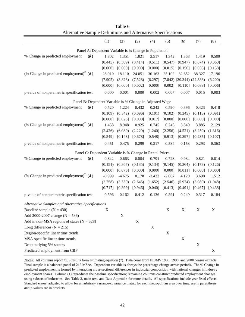
(1) (2) (3) (4) (5) (6) (7) (8)

% Change in predicted employment (β ) 1.802 1.351 1.821 2.517 1.342 1.368 1.419 0.509(0.445) (0.309) (0.414) (0.511) (0.547) (0.947) (0.674) (0.360)

[0.000] [0.000] [0.000] [0.000] [0.015] [0.150] [0.036] [0.158](% Change in predicted employment)2 (δ ) 28.010 18.110 24.051 30.163 25.102 32.652 38.327 17.196

(7.905) (3.823) (7.528) (6.297) (7.842) (20.344) (22.388) (6.200) [0.000] [0.000] [0.002] [0.000] [0.002] [0.110] [0.088] [0.006]

p-value of nonparametric specification test 0.000 0.001 0.000 0.002 0.007 0.007 0.015 0.003

% Change in predicted employment (β ) 0.520 1.224 0.432 0.242 0.590 0.896 0.423 0.418(0.109) (0.542) (0.096) (0.101) (0.102) (0.245) (0.115) (0.091)

[0.000] [0.025] [0.000] [0.017] [0.000] [0.000] [0.000] [0.000](% Change in predicted employment)2 (δ ) 1.458 8.948 0.925 0.745 0.246 3.840 3.885 2.129

(2.426) (6.080) (2.229) (1.240) (2.256) (4.521) (3.259) (1.316) [0.549] [0.143] [0.678] [0.548] [0.913] [0.397] [0.235] [0.107]

p-value of nonparametric specification test 0.451 0.475 0.299 0.217 0.584 0.153 0.293 0.363

% Change in predicted employment (β ) 0.842 0.663 0.804 0.791 0.728 0.934 0.821 0.814(0.151) (0.367) (0.135) (0.134) (0.145) (0.364) (0.173) (0.126)

[0.000] [0.073] [0.000] [0.000] [0.000] [0.011] [0.000] [0.000](% Change in predicted employment)2 (δ ) -0.999 -4.675 0.178 -3.422 -2.087 4.120 3.698 1.512

(2.758) (5.530) (2.645) (1.652) (2.546) (5.974) (5.080) (1.948) [0.717] [0.399] [0.946] [0.040] [0.413] [0.491] [0.467] [0.438]

p-value of nonparametric specification test 0.596 0.162 0.412 0.136 0.591 0.240 0.317 0.184

Alternative Samples and Alternative SpecificationsBaseline sample (N = 430) X X X X XAdd 2000-2007 change (N = 586) XAdd in non-MSA regions of states (N = 528) XLong differences (N = 215) XRegion-specific linear time trends XMSA-specific linear time trends XDrop outlying 5% shocks XPredicted employment from CBP X

Table 6Alternative Sample Definitions and Alternative Specifications

Panel A: Dependent Variable is % Change in Population

Panel B: Dependent Variable is % Change in Adjusted Wage

Panel C: Dependent Variable is % Change in Rental Prices

Notes: All columns report OLS results from estimating equation (7). Data come from IPUMS 1980, 1990, and 2000 census extracts. Final sample is a balanced panel of 215 MSAs. Dependent variable is always the percentage change across periods. The % Change in predicted employment is formed by interacting cross-sectional differences in industrial composition with national changes in industry employment shares. Column (1) reproduces the baseline specification; remaining columns construct predicted employment changes using subsets of industries. See Table 2, main text, and Data Appendix for more details. All specifications include year fixed effects. Standard errors, adjusted to allow for an arbitrary variance-covariance matrix for each metropolitan area over time, are in parenthesis and p-values are in brackets.

42

(1) (2) (3) (4) (5) (6) (7) (8) (9) (10)Transfer Payment Elasticity

Returns to Scale

H0: σ L = σ H

Row Model σ h β h σ H β H σ L β L ψ α σ L – σ H

(1) Baseline Model 1.201 6.306 -0.066 -1.044 -0.065 -0.861 -3.838 1.038 -0.001 21.088(0.407) (1.774) (0.016) (0.766) (0.019) (0.738) (0.447) (0.025) (0.015) [0.515][0.003] [0.000] [0.000] [0.174] [0.001] [0.244] [0.000] [0.129] [0.951]

(2) No Housing; No Transfers 1.009 6.472 -0.107 -0.495 -0.201 -0.900 -4.341 1.020 0.093 25.262(0.432) (2.685) (0.017) (0.408) (0.024) (0.276) (0.577) (0.021) (0.016) [0.285][0.020] [0.016] [0.000] [0.226] [0.000] [0.001] [0.000] [0.336] [0.000]

(3) No Transfers 0.872 5.604 -0.060 -1.060 -0.119 -0.938 -4.256 1.030 0.059 18.881(0.399) (2.517) (0.016) (0.839) (0.022) (0.484) (0.572) (0.023) (0.016) [0.653][0.030] [0.027] [0.000] [0.207] [0.000] [0.053] [0.000] [0.192] [0.000]

(4) No Housing 1.060 6.436 -0.106 -0.504 -0.135 -0.775 -4.225 1.020 0.029 25.593(0.413) (2.478) (0.015) (0.410) (0.019) (0.286) (0.509) (0.020) (0.014) [0.270][0.011] [0.010] [0.000] [0.220] [0.000] [0.007] [0.000] [0.316] [0.042]

(5) s H = s L = 0.33 1.151 6.318 -0.059 -1.141 -0.067 -1.005 -3.889 1.035 0.007 20.406(0.413) (1.875) (0.016) (0.875) (0.019) (0.739) (0.450) (0.024) (0.015) [0.558][0.006] [0.001] [0.000] [0.193] [0.000] [0.174] [0.000] [0.145] [0.611]

(6) σ H,L = 20 2.019 5.844 -0.033 0.847 -0.038 0.495 -3.626 0.994 0.005 25.320(0.654) (1.539) (0.013) (0.443) (0.015) (0.541) (0.455) (0.030) (0.005) [0.282][0.002] [0.000] [0.015] [0.057] [0.016] [0.361] [0.000] [0.849] [0.360]

(7) σ H,L = 0.1 0.601 10.748 -0.065 -1.954 -0.066 -1.334 -3.695 1.236 0.001 38.345(0.221) (2.128) (0.013) (0.810) (0.016) (0.667) (0.410) (0.020) (0.014) [0.017][0.007] [0.000] [0.000] [0.016] [0.000] [0.046] [0.000] [0.000] [0.939]

(8) Alternative Wage Measure 0.662 8.611 -0.032 -3.011 -0.007 -10.391 -3.315 1.062 -0.025 26.389 (Residualized Wages) (0.363) (2.806) (0.010) (1.304) (0.006) (2.715) (0.497) (0.011) (0.011) [0.235]

[0.069] [0.002] [0.003] [0.021] [0.286] [0.000] [0.000] [0.000] [0.026]

(9) Drop Labor Demand Moments 1.209 5.305 -0.085 -0.604 -0.079 -0.089 -4.270 -0.006 11.892(0.700) (3.291) (0.022) (0.692) (0.023) (0.626) (0.448) N/A (0.015) [0.537][0.085] [0.108] [0.000] [0.383] [0.001] [0.887] [0.000] [0.677]

Table 7GMM Estimates of Full Model

Notes: All rows report estimates of the full model using a nonlinear, simultaneous equations GMM estimator. Alternate specifications are presented in each row; parameter estimates are listed in the columns. See Section 6 of main text and Section A.5 of the Online Appendix for more details. Asymptotic standard errors are in parenthesis and p-values are in brackets. In column (8), the p-value reported is for the test of whether the point estimate is statistically significantly different from 1.

Housing Supply Curve

High-Skill Mobility Cost Function

Low-Skill Mobility Cost Function χ 2 test

statistic

43

0L L

w

hspw 00 =

hspw ++ =

BL−

LS

=−w

+L

c

Δ+Δ−

LD

Figure 1: Constant Housing Supply Elasticity

AL−

csp

sp

hB

hA

−−

−

Notes: This figure displays the equilibrium response when the housing supply elasticity is constant. The initialequilibrium wages, labor supply, and housing prices are given by the dot in the center of the figure. An exogenousincrease in wages encourages in-migration until labor supply rises to L+. At this point, housing prices haverisen to completely offset the increase in wages, restoring the no-arbitrage condition for workers. If there areno mobility costs, then the equilibrium response of an equal-sized exogenous decrease in wages is symmetric,as shown by LA

−. If out-migration is costly, however, then following a negative shock, the marginal out-migrantmust be indifferent between staying and paying c to out-migrate. These mobility costs cause both populationand housing prices to respond asymmetrically : positive shocks increase population and housing prices morethan negative shocks reduce them.

44

w

LS

Δ+Δ−

LD

c

Figure 2: Concave Housing Supply Curve

hspw 00 =

hspw ++ =

=−w csp

sp

hD

hC

−−

−

0L LDL− +LCL−

Notes: This figure displays the equilibrium response when the housing supply curve is concave. As the maintext and Appendix describe in more detail, a concave housing supply curve is consistent with a durable housingstock that is not destroyed once created. As in figure 1, the initial equilibrium wages, labor supply, and housingprices are given by the dot in the center of the figure. An exogenous increase in wages encourages in-migrationuntil labor supply rises to L+. At this point, housing prices have risen to completely offset the increase inwages, restoring the no-arbitrage condition for workers. If there are no mobility costs, then housing prices stillrespond symmetrically (pC

−). Intuitively, housing costs still must adjust to exactly offset the wage changes. Onlypopulation responds asymmetrically (as shown by LC

−). If workers have mobility costs, then the asymmetry ofthe population response is even greater (see LD

−), and in this case housing prices also respond asymmetrically.

45

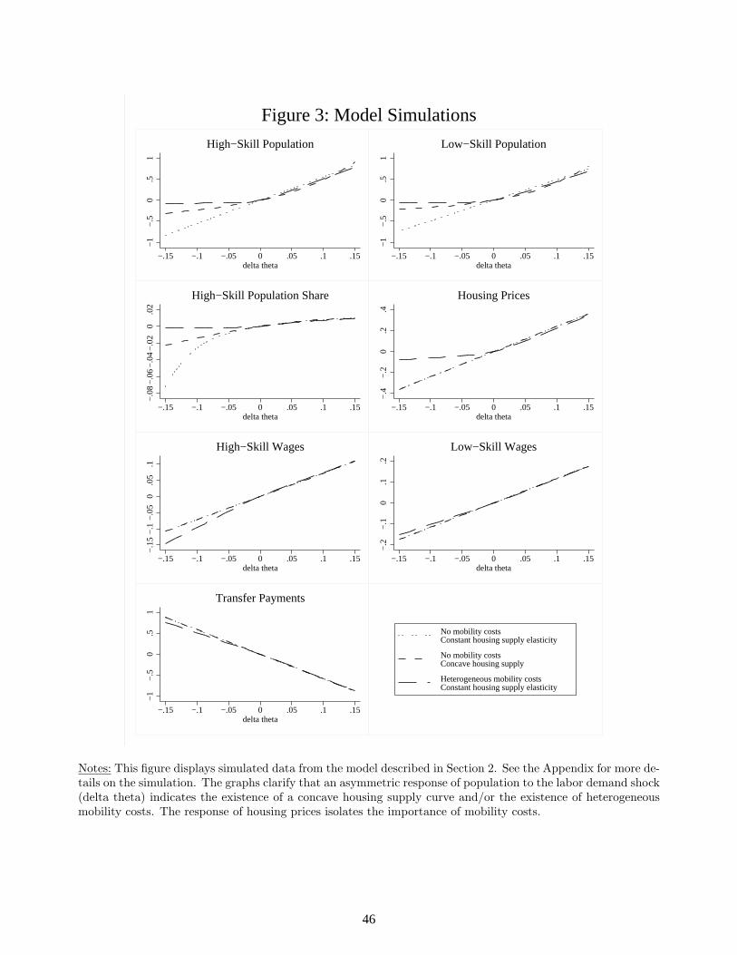
−1

−.5

0.5

1

−.15 −.1 −.05 0 .05 .1 .15delta theta

High−Skill Population

−1

−.5

0.5

1

−.15 −.1 −.05 0 .05 .1 .15delta theta

Low−Skill Population−

.08

−.0

6−

.04

−.0

20

.02

−.15 −.1 −.05 0 .05 .1 .15delta theta

High−Skill Population Share

−.4

−.2

0.2

.4

−.15 −.1 −.05 0 .05 .1 .15delta theta

Housing Prices

−.1

5−

.1−

.05

0.0

5.1

−.15 −.1 −.05 0 .05 .1 .15delta theta

High−Skill Wages

−.2

−.1

0.1

.2

−.15 −.1 −.05 0 .05 .1 .15delta theta

Low−Skill Wages

−1

−.5

0.5

1

−.15 −.1 −.05 0 .05 .1 .15delta theta

Transfer Payments

No mobility costsConstant housing supply elasticity

No mobility costsConcave housing supply

Heterogeneous mobility costsConstant housing supply elasticity

Figure 3: Model Simulations

Notes: This figure displays simulated data from the model described in Section 2. See the Appendix for more de-tails on the simulation. The graphs clarify that an asymmetric response of population to the labor demand shock(delta theta) indicates the existence of a concave housing supply curve and/or the existence of heterogeneousmobility costs. The response of housing prices isolates the importance of mobility costs.

46

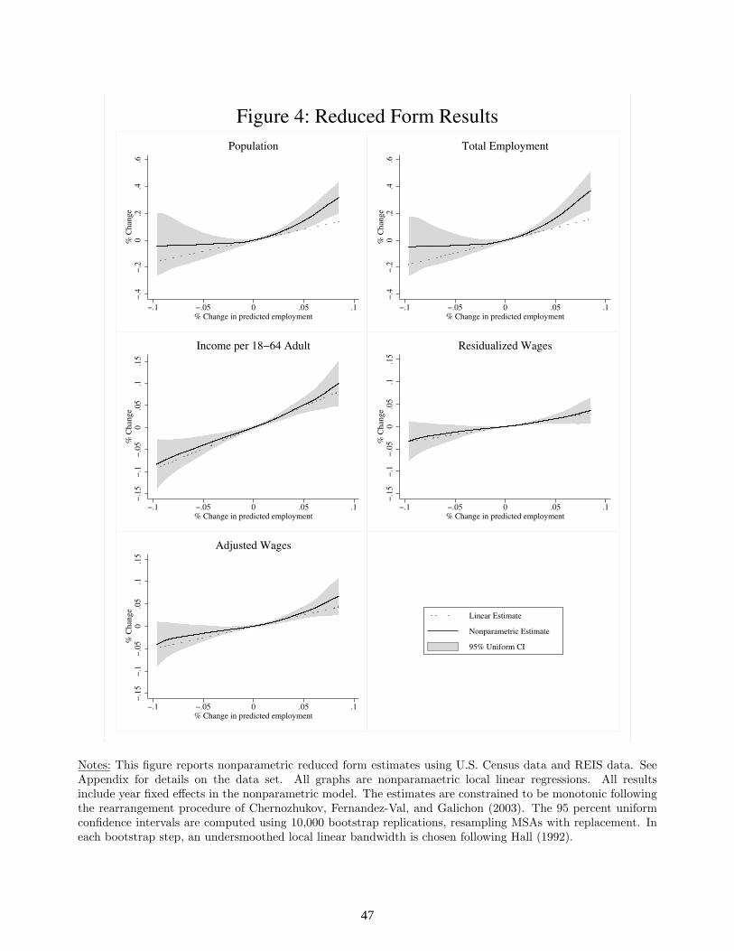
−.4

−.2

0.2

.4.6

% C

hang

e

−.1 −.05 0 .05 .1% Change in predicted employment

Population

−.4

−.2

0.2

.4.6

% C

hang

e

−.1 −.05 0 .05 .1% Change in predicted employment

Total Employment−.

15−.

1−.

050

.05

.1.1

5%

Cha

nge

−.1 −.05 0 .05 .1% Change in predicted employment

Income per 18−64 Adult

−.15

−.1

−.05

0.0

5.1

.15

% C

hang

e

−.1 −.05 0 .05 .1% Change in predicted employment

Residualized Wages

−.15

−.1

−.05

0.0

5.1

.15

% C

hang

e

−.1 −.05 0 .05 .1% Change in predicted employment

Adjusted Wages

Linear Estimate

Nonparametric Estimate

95% Uniform CI

Figure 4: Reduced Form Results

Notes: This figure reports nonparametric reduced form estimates using U.S. Census data and REIS data. SeeAppendix for details on the data set. All graphs are nonparamaetric local linear regressions. All resultsinclude year fixed effects in the nonparametric model. The estimates are constrained to be monotonic followingthe rearrangement procedure of Chernozhukov, Fernandez-Val, and Galichon (2003). The 95 percent uniformconfidence intervals are computed using 10,000 bootstrap replications, resampling MSAs with replacement. Ineach bootstrap step, an undersmoothed local linear bandwidth is chosen following Hall (1992).

47

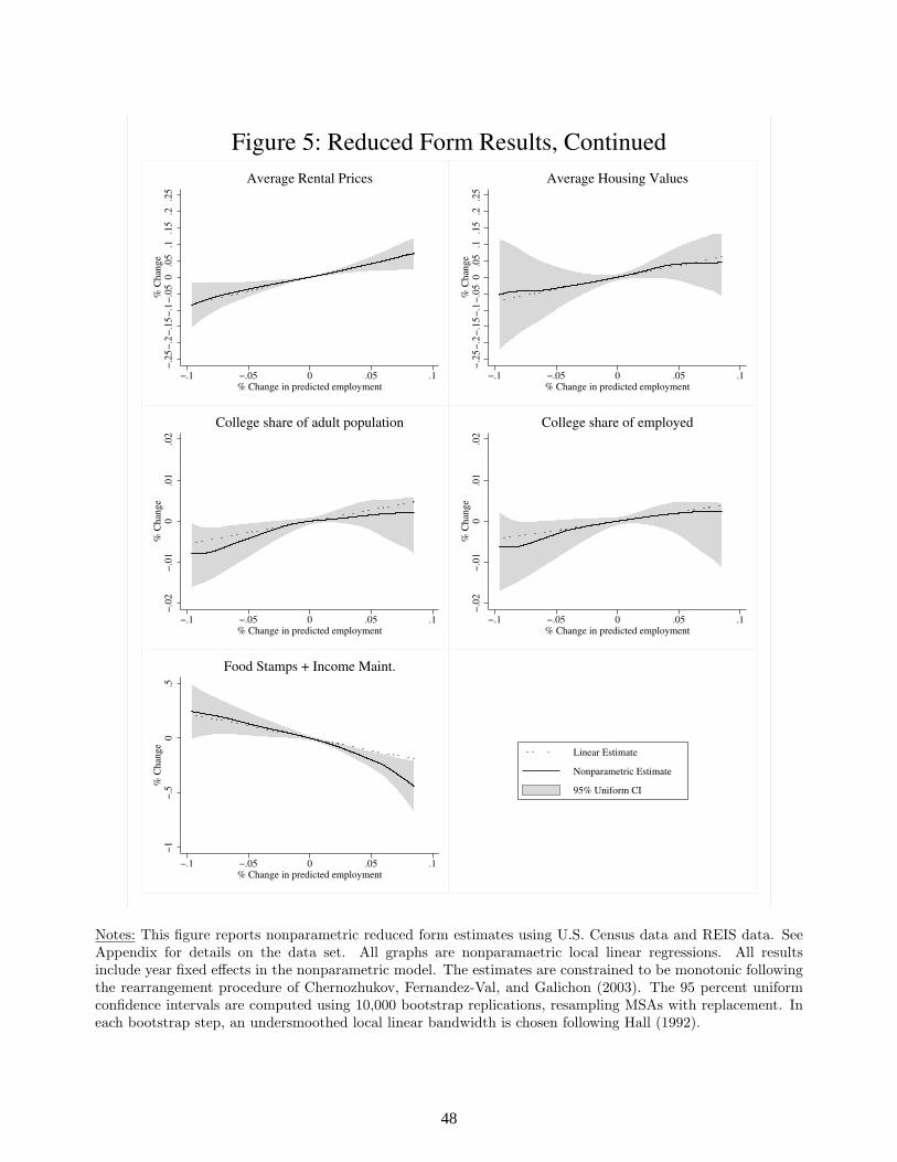
−.25

−.2−

.15−

.1−.

050

.05

.1.1

5.2

.25

% C

hang

e

−.1 −.05 0 .05 .1% Change in predicted employment

Average Rental Prices

−.25

−.2−

.15−

.1−.

050

.05

.1.1

5.2

.25

% C

hang

e

−.1 −.05 0 .05 .1% Change in predicted employment

Average Housing Values−.

02−.

010

.01

.02

% C

hang

e

−.1 −.05 0 .05 .1% Change in predicted employment

College share of adult population

−.02

−.01

0.0

1.0

2%

Cha

nge

−.1 −.05 0 .05 .1% Change in predicted employment

College share of employed

−1−.

50

.5%

Cha

nge

−.1 −.05 0 .05 .1% Change in predicted employment

Food Stamps + Income Maint.

Linear Estimate

Nonparametric Estimate

95% Uniform CI

Figure 5: Reduced Form Results, Continued

Notes: This figure reports nonparametric reduced form estimates using U.S. Census data and REIS data. SeeAppendix for details on the data set. All graphs are nonparamaetric local linear regressions. All resultsinclude year fixed effects in the nonparametric model. The estimates are constrained to be monotonic followingthe rearrangement procedure of Chernozhukov, Fernandez-Val, and Galichon (2003). The 95 percent uniformconfidence intervals are computed using 10,000 bootstrap replications, resampling MSAs with replacement. Ineach bootstrap step, an undersmoothed local linear bandwidth is chosen following Hall (1992).

48

−.4

−.3

−.2

−.1

0.1

.2.3

.4%

Cha

nge

in H

ousi

ng P

rice

−.2 0 .2 .4 .6 .8 1 1.2 1.4% Change in Housing Quantity

Estimated Housing Supply Curve

−.0

8−

.04

0.0

4.0

8M

obili

ty C

ost

−.2 −.1 0 .1 .2% Change in High−Skill Population

Preferred Specification Ignore Transfers

Ignore Housing Ignore Housing, Transfers

High−Skill WorkersEstimated Mobility Cost Function

−.0

8−

.04

0.0

4.0

8M

obili

ty C

ost

−.2 −.1 0 .1 .2% Change in Low−Skill Population

Preferred Specification Ignore Transfers

Ignore Housing Ignore Housing, Transfers

Low−Skill Workers

Estimated Mobility Cost Function

Figure 6: GMM Estimates

Notes: This figure reports GMM estimates of the full model. The top figure presents the housing supply curvethat is estimated in the baseline model (Table 7, row 1). The middle and bottom figures report estimatedmobility functions under various assumptions about housing expenditure shares and transfer payments. SeeSection 6 and the Appendix for more details on the GMM estimation.

49

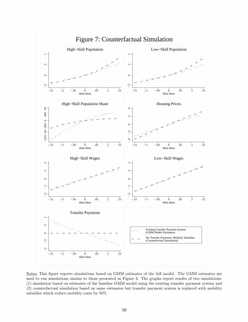
−.5

0.5

1

−.15 −.1 −.05 0 .05 .1 .15delta theta

High−Skill Population

−.5

0.5

1

−.15 −.1 −.05 0 .05 .1 .15delta theta

Low−Skill Population−

.015

−.0

1−.0

050

.005

.01

−.15 −.1 −.05 0 .05 .1 .15delta theta

High−Skill Population Share

−.4

−.2

0.2

.4

−.15 −.1 −.05 0 .05 .1 .15delta theta

Housing Prices

−.2

−.1

0.1

.2

−.15 −.1 −.05 0 .05 .1 .15delta theta

High−Skill Wages

−.2

−.1

0.1

.2

−.15 −.1 −.05 0 .05 .1 .15delta theta

Low−Skill Wages

−1

−.5

0.5

1

−.15 −.1 −.05 0 .05 .1 .15delta theta

Transfer Payments

Existing Transfer Payment System(GMM Model Estimates)

No Transfer Payments, Mobility Subsidies(Counterfactual Simulation)

Figure 7: Counterfactual Simulation

Notes: This figure reports simulations based on GMM estimates of the full model. The GMM estimates areused to run simulations similar to those presented in Figure 3. The graphs report results of two simulations:(1) simulation based on estimates of the baseline GMM model using the existing transfer payment system and(2) counterfactual simulation based on same estimates but transfer payment system is replaced with mobilitysubsidies which reduce mobility costs by 50%.

50

0.0

5.1

.15

Sha

re o

f sam

ple

−.16 −.12 −.08 −.04 0 .04 .08 .12 .16% Change in predicted employment

Appendix Figure A1: Symmetry of Predicted Employment Shock

Notes: This figure displays a histogram of the local labor demand shock used throughout the paper. Thesymmetry of the distribution of the shock implies that the estimated asymmetric responses are not due (inpart) to underlying asymmetries in the shock itself.

51