Munich Personal RePEc Archive

The Implication of Monetary and Fiscal

Policy Interactions for the Price Levels:

the Fiscal Theory of the Price Level

Revisited

Assadi, Marzieh

1 October 2017

Online at https://mpra.ub.uni-muenchen.de/84851/

MPRA Paper No. 84851, posted 02 Mar 2018 17:46 UTC

1

The Implication of Monetary and Fiscal Policy Interactions for the

Price Levels: The Fiscal Theory of the Price Level Revisited

Marzieh Assadi 1 Faculty of Social Science, the University of Golestan

This Version: October 2017

Abstract

This paper contributes to the empirical literature on the interaction between monetary and fiscal

policy. We consider the impact of monetary and fiscal policy shocks on inflation and output

dynamics using a Time-Varying Parameter Factor-Augmented VAR (TVP-FAVAR) method. In

baseline results from a linear model, including fiscal policy in the factors has implications for the

impact of monetary policy shocks on inflation. This can be explained by wealth effects. The

wealth effect is the change in spending that accompanies a change in perceived wealth. Hence,

increases in interest rates increase the wealth of bondholders. Moreover, results from our TVP-

FAVAR indicate that price puzzles from monetary policy shocks are more accentuated during

particular regimes. For example, under an active fiscal policy and passive monetary policy,

inflation rose in response to a contractionary monetary policy shock. The underlying mechanism

can be explained through the wealth channel. Finally, the results of a fiscal expansion provide

support for the non-Ricardian view on fiscal policy within both the linear and non-linear FAVAR

model. That is, inflation and output both responded to the fiscal shock.

Keywords: Monetary and Fiscal Policy Interaction, Ricardian Equivalence, Fiscal Theory of the Price Level, Price Puzzle, Time-Varying Parameter Factor-Augmented VAR (TVP-FAVAR). JEL Classification Codes: E52; E62; E63; E65.

Acknowledgment: I would like to thank Ben S. Bernanke, Jean Boivin, Piotr Eliasz, Gary Koop,

and Dimitris Korobilis for making available their FAVAR and TVP-FAVAR Matlab code.

1 Corresponding Author; E-mail address: asaadi.m@gmail.com

2

1.1 Introduction

This paper studies the interactions between monetary and fiscal policy in the United States.

Before the Global Financial Crisis of 2008, the consensus view of mainstream macroeconomics

was that monetary policy should actively respond to inflation using the nominal interest rate. In

contrast fiscal policy should have a less activist role and passively respond to the business cycle

using automatic stabilisers, while focusing upon balancing the government budget, see Walsh

(2010). During the Great Recession however, the United States actively responded to the

economic downturn using both monetary and fiscal policy. Consequently, the mainstream view

was called into question and the interactions between monetary and fiscal policy became much

more important. Moreover, sovereign debt levels have grown significantly after the Great

Recession. For example, US Central Government Debt as a percentage of GDP has grown from

just over 50% at the start of the millennium to over 100% recently, see Figure 3.1. Consequently,

this debt build up may present substantial challenges for the conduct of monetary policy in more

normal times, see Reinhart and Rogoff (2010) for a detailed discussions. In addition, fiscal policy

is potentially important in influencing aggregate demand and inflation. This has recently been

argued in Chung et al. (2007), Davig and Leeper (2007, 2011), and Sims (2011) that monetary

policy should not be examined in isolation from fiscal policy.

As discussed in Paper 2, the standard theoretical view is that monetary policy affects

aggregate demand, and hence output and inflation in the short-run. According to Keynesian,

Monetarist, and New Keynesian models changes in Central Bank nominal interest rate may lead

to changes in real rates and therefore economic activity.1 The latter emphasizes the importance

of interest rate rules as a way of controlling inflation. Central Banks operating with discretion

have a tendency to deviate from low inflation leading to an inflation bias in policy. Kydland and

Prescott (1982) outline these incentives and emphasize the role of Central Bank credibility and

1 According to monetarists view monetary aggregates is the main determinant of inflation. The monetarists view is synthesized by Milton Friedmanˈs famous dictum that "inflation is always and everywhere a monetary phenomenon", see Leeper and Walker (2012).

3

pre-commitment in resolving the bias of policy. Ultimately, Rogoff (1985) emphasised monetary

policy should be implemented by an independent Central Bank which would in turn separate

monetary and fiscal policy.

In contrast, fiscal policy must reliably adjust surpluses to ensure that government debt is

stable and fiscal policy should not seek to actively influence aggregate demand, see Walsh

(2010), and Canzoneri et al. (2011). Ricardian Equivalence between debt and taxes suggests

fiscal policy does not influence consumption. In the case that fiscal policy generates government

debt, the issuance of new bonds to finance the incurred debt would imply additional taxes in the

future; hence, bonds do not represent net wealth. However, we can also contrast this position

with the non-Ricardian view: the fiscal authority sets the government budget regardless of

intertemporal budget constraint. It implies that the monetary authority is forced to fully

accommodate a fiscal deficit by financing the incurred debt with current and future money

creation. Thus, any change in the current stock of debt indicates future money growth, see

Aiyagari and Gertler (1985), Woodford (1996, 1998), Christiano and Fitzgerald (2000),

Canzoneri et al. (2011), and Sims (1994, 2013).

An alternative approach to understand why fiscal policy can be important for inflation

dynamics is the Fiscal Theory of the Price Level (FTPL). As discussed in Paper 2, the FTPL was

introduced by Sargent and Wallace (1981) in their famous paper on Unpleasant Monetarist

Arithmetic, and developed further by Cochrane (1999, 2001, 2009), Leeper (1991, 2013), Sims

(1994, 1997, 2011), and Woodford (1996, 1998). The FTPL points to the possibility of an

independent role for the fiscal stance in determining and controlling inflation. While the

monetary-focused literature deems that fiscal policy must reliably adjust to ensure governmentˈs

debt sustainability, the FTPL counter argues that there are situations when the Central Bank does

not target inflation due to other concerns, such as output stabilization or a financial crisis. In these

circumstances, monetary policy may lose its credibility to control inflation and influence the real

4

economy in the conventional way, see Chung et al. (2007), Davig and Leeper (2007), Sims

(2011), Leeper and Walker (2012), and Leeper (2013).

Moreover, it is important to consider that monetary and fiscal policy interactions may

change over time depending upon the macroeconomic framework. We can contrast two different

regimes in particular in which monetary and fiscal policy interacts, see Leeper (1991) and

Woodford (1996). Firstly, an active monetary policy and a passive fiscal policy, when the Central

Bank responds to inflation and the fiscal authority satisfies the budget constraint. Secondly, a

passive monetary policy and an active fiscal policy, when the fiscal authority independently

determines its budget while the Central Bank is required to adjust monetary policy in order to

satisfy the government budget constraint.2,3,4

Much of the monetary-focused literature considers the fiscal stance irrelevant for achieving price

stability, as long as the governmentˈs intertemporal budget constraint is satisfied. However, the

fiscal authority’s decision can influence the impact of monetary policy. Bradley (1984), Sims

(1994), Cochrane (1999), Canzoneri et al. (2011), Davig and Leeper (2011), Sims (2011), and

Leeper and Walker (2012) discuss that the omission of the fiscal stance from models intended to

evaluate monetary policy may produce inferior results, i.e. omitted variable bias. The reason is

that fiscal variables can be a key source for changes in inflation, see Sims (2011).5 To illustrate

the important implication of fiscal and monetary policy interactions for the determination of the

2 As discussed in Paper 2, Woodford (1996) describes active monetary and passive fiscal policy case as the Ricardian because monetary shocks can change the price levels without involving the fiscal stance. This is generally considered as the conventional outcome. In contrast, the second case of passive monetary and active fiscal policy is the Non-Ricardian as the fiscal stance does impact the price levels by encouraging private expenditure. 3 The importance of government liabilitiesˈ finance-source for the analysis of the inflation is first initiated by Sargent and Wallace (1981), and Sargent (1982). 4 According to Sargent and Wallace (1981) when government deficits are considered as exogenous, monetary

policy loses its ability to control inflation when the deficits reach the fiscal limit. It puts pressure on the monetary authority to generate seigniorage revenues for government to ensure the interest payments on the debt. In contrast to the idea that fiscal inflation is caused by monetizing deficits in Sargent and Wallace (1981), the FTPL relates the nominal bond to a nominal payoff in which the real value of the payoff depends on the price level. When the nominal debt is fully financed by real resources, i.e. real primary surplus and seigniorage, fiscal policy is inflationary only if the Central Bank monetizes deficits. However, when the government does not increase the real resources to finance the debt, the FTPL creates a direct link between current and expected deficits and inflation, see Leeper (2013). 5 Sims (2011) provides a theoretical discussion of the way that fiscal authorities decisionˈs may impact the monetary transmission mechanism. He concludes that if a Central Bank aims to consider all the factors that impact inflation and output growth, they should not ignore the fiscal stance.

5

price level, Leeper (1991, 2013) argues that to ensure the uniqueness of equilibrium, either

monetary or fiscal policy must be active and the other one passive.

This paper studies the impact of monetary policy on output growth and inflation, whilst

accounting for the potential role for the governmentˈs fiscal stance. Earlier empirical evidence on

monetary and fiscal policy interactions comes from either the VAR models or Structural Policy

Rules approach, see Favero and Monacelli (2003), Davig and Leeper (2007), and Canzoneri et al.

(2011) among others. As mentioned in Paper 2, VAR models have been developed as one of the

key empirical tools for analysing policy and evaluating theory.6 One major problem concerns

VAR models, however, is the occurrence of the puzzling behaviour of some Impulse Response

Functions (IRF), with the price puzzle as the most common one. The price puzzle is an increase

in the price level in response to a contractionary monetary policy shock. The dominant view in

the literature relates the puzzle to the curse of dimensionality concerns VAR models to maintain

the degree of freedom.7,8 The curse of dimensionality is that as the dimension of the system

increases the number of parameters to be estimated grows. This exhausts the available degree of

freedom even for large datasets, see Sims (1980).

Several studies attempt to resolve the puzzle by changing the identification assumptions or by

expanding the information set on which policy choices are based.9 However, Hanson (2004)

argues that the price puzzle was more pronounced in the 1960s and the 1970s, which is considered

to be a period of active fiscal policy and passive monetary policy. This implies that the price

puzzle may be explained through the way in which monetary and fiscal policy interacts and

influences inflation rather than adding extra information to the model.10 Chung et al. (2007) argue

6 See, Bernanke and Blinder (1992), Bernanke and Boivin (2003), Bernanke et al. (2005), Del Negro and Schorfheide (2010), and Koop and Korobilis (2010). 7Sims (1992) first commented on the price puzzle as an unconventional response of the price level to a monetary contraction. The "price puzzle" was named by Eichenbaum (1992). Sims (1992) explains that the price puzzle occurs as a result of imperfect information that the Central Bank may use to predict the future inflation. 8 Hanson (2004) provides a comprehensive survey on the price puzzle literature. One most common interpretation for the price puzzle relates it to the VAR misspecification which would be either disappear or lessen by adding further information to the estimated VAR. 9 See Bernanke et al. (2005) for a detailed discussion. 10 Another explanation for the price puzzle relates the counterintuitive reaction of prices to a monetary contraction to the cost channel of monetary transmission which impacts the supply-side of the economy as opposed to the

6

that the price puzzle that emerges in monetary VARs can be a natural outcome of periods when

an active fiscal policy coordinates with a passive monetary policy, rather than the identification

problems.

Recently, Factor-Augmented VAR models appear to help deal with the counter-intuitive price

puzzle to some extent by incorporating additional information into the VAR, see Bernanke and

Boivin (2003), Bernanke et al. (2005), and Stock and Watson (2005). However, FAVAR models

are typically linear and it is difficult to justify this approach in the presence of changes in

macroeconomic policy regimes. For example, there exists evidence of substantial fiscal regime

instability, see Favero and Monacelli (2003), Chung et al. (2007), and Davig and Leeper (2007,

2011). Favero and Monacelli (2003) argue that the constant-parameter analysis of fiscal policy

studies would be misleading in that it would predict a stabilizing fiscal regime throughout the

sample. These arguments motivate us to employ a non-linear Time Varying Parameter approach

to study the macroeconomic impact of monetary and fiscal policy interactions.

The non-linear analysis of VAR models first proposed by Primiceri (2005), namely TVP-VAR,

to consider monetary shocks at different points in time. Another alternative to TVP-VAR method

is the Regime-Switching models as proposed by Sims and Zha (2006). These models are

developed to capture a determinant finite number of breaks representing rapid shifts in the

policy.11 One clear advantage of TVP models over the Regime-Switching approaches is that TVP

models capture smooth changes of the coefficients over time, see Primiceri, (2005).

The idea of combining the FAVAR models with TVP was developed by Koop and Korobilis

(2010), and Korobilis (2013). This has proved successful in addressing the problems associated

with standard VAR models. That is low dimensionality and non-linear regimes. Comparing the

results obtained from a Constant-Parameter FAVAR model in Bernanke et al. (2005) with those

demand-side, see Barth and Ramey (2002). The cost channel explains that to the extent that firms must borrow to finance the cost of production and new investment, higher interest rates increase the unit cost that induces an increase in the price level at least for some periods, see Barth and Ramey (2002), and Christiano et al. (2005). 11 As explained in Primiceri (2005), the learning dynamics of the agents and the monetary authority can be better captured by a model with smooth and continuous drifting coefficients rather than a model with discrete breaks.

7

presented in Korobilis (2013) from a TVP-FAVAR model, it is clear that the latter approach

corrects the price puzzle to a greater extent.

However, despite the promising results obtained from different combination of TVP and FAVAR

methods to address the price puzzle, the potential impact of the fiscal stance on the economy has

been ignored, see Bernanke et al. (2005), Primeciri (2005), Sims and Zha (2006), Koop and

Korobilis (2010), and Korobilis (2013) among others. Table 3.1 presents a summary of the related

literature in which this Paper is closely related with. It shows that the empirical literature on the

monetary transmission mechanism mainly relies on a Ricardian interpretation of the fiscal

policy.12

We identify a gap in the literature on both the monetary transmission mechanism, and monetary

and fiscal policy interactions. While the former studies the impact of monetary policy on the real

activity measures isolated from fiscal policy, the latter one provide evidence on the

macroeconomic policy interactions within small VAR models. Thus, this Paper contributes to the

empirical literature on monetary and fiscal policy interactions in the following ways. Firstly, we

examine monetary-fiscal policy interactions by examining the responses to a monetary shock in

a FAVAR model including fiscal policy variables. Secondly, we compare whether monetary

policy interactions change over time. We do so by using a TVP-FAVAR model, which accounts

for different periods of monetary and fiscal dominance. Thirdly, we examine the macroeconomic

impact of fiscal policy shock within both a linear and non-linear FAVAR model.

To preview our results, firstly we find that including fiscal variables in the baseline linear

FAVAR causes an increase in inflation in response to a contractionary monetary policy shock.

This response can be explained through a wealth effect. In the presence of government debt, a

higher interest rate can stimulate private expenditure, as agents may perceive an increase in their

12 The monetary-focused literature on the transmission mechanism of monetary policy ignores the impact of the fiscal stance on the economy and implicitly assumes that fiscal policy can only change the composition of GDP rather than its level, see Table 3.1.

8

wealth, i.e. the issuance of new bonds or an increase in their disposable income. This in turns can

encourage private consumption leading to an increase in aggregate demand and inflation.

Second, the results from the TVP-FAVAR model suggest that the fiscal-augmented model

produce price puzzles. The mechanism works as follows. Higher interest rates induce

bondholders to consume more in periods when fiscal policy is active. As defined in Paper 2, an

active fiscal policy means that the fiscal authority determines taxes and government expenditure

independent of inter-temporal budget constraint. This finding provides evidence for the role of

fiscal policy on the price determinations. The influence tends to be more accentuated in the case

of an active fiscal and passive monetary policy as higher interest rates can lead to the issuance of

more government bonds. This would increase government debt given that an active fiscal policy

is in place. Thus, the outcome of a monetary contraction can be an increase in private

consumption through a positive wealth effect. Third, the non-Ricardian view on the fiscal policy

can find empirical support within both Constant and TVP-FAVAR models as both inflation and

output increase in response to the fiscal shock.

Thus, the main contribution of this paper is to empirically validate the alternative interpretation

of the price puzzle explained in Chung et al. (2007). This fiscal interpretation differs from the

Cost-Channel explanation of the price puzzle initiated by Barth and Ramey (2002), and

Christiano, Eichenbaum, and Evans (2005). Our study, also, confirms the empirical inference

drawn by Favero and Monacelli (2003), Davig and Leeper (2007, 2011), and Leeper and Walker

(2012), Leeper (2013) on the non-Ricardian view of fiscal policy in the United States. Finally, as

regards the outcome of monetary contractionary policy shock within a fiscal-excluded TVP-

FAVAR model, our results are consistent with those presented in Korobilis (2013) in mitigating

the price puzzle. The paper is organised as follows. Section 3.2 is a brief review of the related

literature. In section 3.3, the econometric methodology is explained. Section 3.4 presents model

specifications and the empirical results. A brief summary of results is provided in section 3.5.

Section 3.6 concludes the study.

9

Table 3.1. Key Literature on Monetary and Fiscal Policy Study Methodology Monetary-Fiscal

Policy Interactions

Main Contribution

Bernanke, Boivin, and Elliasz (2005)

FAVAR Monetary-Focused The appearance of the price puzzle is due to the lack of information. Their results show that adding extra information can reduce the price puzzle.

Primiceri (2005) TVP-VAR Monetary-Focused Non-Systematic shocks may better explain the peaks in inflation over the 1970s and 1980s rather than weaker interest rate responses to inflation and real activity.

Korobilis (2013) TVP-FAVAR Monetary-Focused Firstly, the responses of output, investment, and quantity of money to monetary shocks have been changed over the time. Secondly, the constructed TVP-FAVAR can correct the price puzzle to a great extent compared with those of Bernanke et al. (2005).

Favero and Monacelli (2003)

Markov-Switching VAR-Augmented Policy Rules

Monetary-Fiscal Policy does interacts

Monetary and fiscal policy interactions have inflationary effects. In addition, fiscal policy appears to perform as the non-Ricardian before 1987, while it turns to be Ricardian after 1987.

Chung, Davig, and Leeper (2007)

Markov-Switching Policy Rules

Monetary-Fiscal Policy does interacts

The price puzzle can be a natural outcome of an active fiscal policy and a passive monetary policy. In addition, under this macroeconomic policy coordination, the Ricardian view on policy interactions appears to be implusible.

Davig and Leeper (2007,2011)

Markov-Switching Policy Rules

Monetary-Fiscal Policy does interacts

The outcome of an active fiscal policy and a passive monetary policy is the non-Ricardian. That is inflation and output increase in response to a fiscal expansion by generating a positive wealth effect which encourage private consumption.

Note: This Table summarizes the related literature that the paper is constructed upon it.

10

1.2 Review of the Literature on Monetary and Fiscal Policy Interactions

The general consensus on the dominant role of monetary policy has recently been subject to

critique. Indeed, monetary and fiscal policy do interact through the intertemporal government

budget. However, the government budget can be considered either as a constraint or as an

equilibrium condition upon different monetary and fiscal policy coordination, see Favero and

Monacelli (2003), Walsh (2010), Leeper and Walker (2011), Sims (2011), and Leeper (2013)

among others. This suggests that the Ricardian view on fiscal policy, which assumes fiscal policy

is ineffective and the government budget is a constraint, is difficult to justify as a fact that can be

held under all circumstances.

Despite the existence of a vast literature on the impact of monetary policy on the economy,

monetary studies often neglect to consider the potential role for fiscal policy in their analysis.13

The empirical literature on the transmission of monetary policy shocks is mainly studied through

VAR modelling.14 This literature mainly studies the effect of unanticipated monetary policy

shocks that are constructed using VAR models, assuming that the specified VAR models contain

the present and past information of the agents. For example, much research attempts to investigate

the cause of the US inflation in the 1970s, concludes that it can be explained by misconduct of

monetary policy and that inflation is induced by a rapid growth of the money supply. Christiano

et al. (1999) provide a comprehensive survey of the literature.

In contrast, Sims (1994, 2011) argues that in a fiat-money economy, inflation appears to be more

a fiscal phenomenon rather than a monetary one, given that the value of fiat money always

depends on public beliefs about future fiscal policy. Furthermore, when there is uncertainty about

future fiscal policy, a monetary policy instrument may lose its influence on the economy, or

produces unconventional effects such as the price puzzle.

13 The exceptions are noted in Paper 2. 14 Another alternative approach to study the monetary transmission mechanism is Structural Policy Rules approach. The literature in this area is built and developed mainly based on Taylor (1993) in a way that the policy rules reflects systematic response of monetary policy to exogenous shocks. These studies focus on examining monetary policy as systematic response to variation in observable variables within the estimated Structural Policy Equations, see for example Clarida et al. (2000).

11

Sims (2011) explains that a debt-financed fiscal expansion, can account for volatility in US

inflation over the sample 1960-2010.15 He shows that an expansionary fiscal policy shock under

an active fiscal policy and a passive monetary policy induces inflation and consumption to

increase.16 Accordingly, Sims (2011) suggests that the econometric models intended to analyse

monetary policy should explicitly involve the fiscal stance, as this may be a primary cause of

inflation.

Having said that fiscal policy is an important factor for the determination of inflation, the literature

on the macroeconomic impact of fiscal policy is divided between two views, namely the

Ricardian, and non-Ricardian. The empirical literature on the impact of fiscal policy supports the

both views.17 Examples for the Ricardian view include Barro (1979), Evans (1985,1987), Plosser

(1987), Bohn (1998), and Canzoneri et al. (2001, 2011).18 In an empirical study, Bohn (1998)

examined the US fiscal policy and concluded that a rise in the debt-to-GDP ratio leads to an

increase in the primary surplus and taxes respond to ensure that the intertemporal budget

constraint is satisfied. According to his findings, fiscal policy appears to act in a Ricardian way.

In another study, Canzoneri et al. (2011) examine the response of US liabilities to a positive shock

to the primary surplus within a VAR model. They argue that a positive shock to the primary

surplus can reduce real liabilities without negative correlation. Thus, they provide evidence

supporting a Ricardian interpretation for fiscal policy in the sense that output and inflation is

unresponsive to fiscal policy shocks. In contrast, a monetary contraction causes output and

15 The results presented in Sims (2011) come from a structural VAR consists of real GDP, the personal consumption expenditure, price deflator, one-year US treasury rate, the 10-year treasury rate, the ratio of the primary deficit to the market value of privately held US government debt, the market value of privately held US government debt divided by nominal GDP, and interest expenses as a fraction of total receipts in the US federal budget. 16 As explained in Paper 2, an active fiscal policy refers to the situation in which the fiscal authority sets its expenditure without taking into account the governmentˈs intertemporal budget equation. It implies that tax revenues are not sufficient to finance the expenditure. A passive monetary policy implies that the monetary authority weakly adjusts the nominal interest rates in response to inflation. 17 As explained in Paper 2, the Ricardian view on fiscal policy states that an expansionary fiscal policy which generate debt implies higher taxes in the future to finance debt. Given that this policy only postpones the tax burdent and does not remove it, the outcome would be an increase in private saving rather than private expenditure. Thus, the policy cannot stimulate the economy. In contrast, a non-Ricardian fiscal policy holds that fiscal policy can effectively stimulate the economy by encouraging private expenditure, see Elmendorf and Mankiw (1999), and Christiano and Fitzgerald (2000). 18 Bernheim (1987) provides a critical survey of the empirical literature on the non-Ricardian view to support the Ricardian view on fiscal policy.

12

inflation to fall as higher interest rate would lower aggregate demand through a reduction in

private expenditure.

In contrast, several other studies show that a debt-financed fiscal expansion can be an effective

policy to increase inflation and output that is a non-Ricardian view on fiscal policy. For example,

Cochrane (2001, 2009) provide a non-Ricardian explanation for government debt dynamics in the

post-war US data. Reade (2011) offers a non-Ricardian interpretation for fiscal policy in response

to the 2008 financial crisis. Sims (2011) argues that the non-Ricardian view on fiscal policy can

explain the high inflation of the 1970s and the early 1980s in the US economy. Davig and Leeper

(2007) find that a monetary contraction combined with a fiscal expansion in which taxes do not

respond sufficiently to debt, can induce a positive wealth effect leading to an increase in private

consumption. This, in turns, would increase inflation and output. Note that the increase in interest

rate induced by the monetary contraction may cause the incurred deficit more expensive to

finance, thus more government liabilities needs to be issued. Until the price levels start to increase,

the new issued bonds would create a positive wealth effect. Moreover, with sticky prices the

wealth effect would stay for some time to affect householdsˈ consumption.

As another example from the literature that accounts for the role of fiscal policy in the monetary

transmission, we can refer to Bradly (1984). He estimates two semi-structural equations

representing the demand and supply equations for reserves to examine the influences of fiscal

policy on monetary policy.19 Bradly (1984) finds that during 1970s-1980s monetary policy does

react to fiscal policy both directly, i.e. through changing the reserves, and indirectly, i.e. through

changing the nominal interest rates. He concludes that the government deficits induce an increase

in money demand due to increasing the public demand for bonds. Consequently, the monetary

authority would be forced to accommodate the growth in money demand.

19 The demand representative equation relates the Fed funds rate to non-borrowed reserves, government debt, and other demand determining variables. The supply equation is a Federal Reserve reaction function which determines the supply of reserves.

13

Given that the outcome of fiscal policy depends on the way that the governmentˈs intertemporal

budget constraint is satisfied, i.e. the Ricardian and non-Ricardian views, different monetary and

fiscal policy regimes also contribute to the outcome. In a seminal paper, Leeper (1991) argues

that under an active monetary policy and a passive fiscal policy regimes, the monetary authority

targets nominal interest rate and does not respond to the governmentˈs debt. In this case, the fiscal

authority would adjust taxes to ensure the governmentˈs intertemporal budget requirements. In

contrast, an active fiscal policy and a passive monetary policy suggests that the monetary

authority adjusts seigniorage revenues to satisfy the governmentˈs budget balance while the fiscal

authority remains unresponsive to the debt.20

Having said that different monetary and fiscal policy regimes may substantially change the policy

outcome, it is also crucial that macroeconomic policy analysis accounts for the potential policy

changes. The literature on monetary and fiscal policy interaction provides evidence for monetary

and fiscal policy regime changes. For example, Favero and Monacelli (2003) estimate fiscal

policy regime changes, using a Markov-switching VAR model, to illustrate the post-war US

inflation and output dynamics. They find that fiscal policy has been active before 1987 and then

switched to passive until 2001.21 They also find that the behaviour of fiscal policy has changed

over the time: after a prolonged period of fiscal policy instability, it switches to a stable period in

1986:Q3 with a Ricardian feature coupled with an active monetary policy. In addition, they

provide evidence that fiscal policy significantly influences the price level when fiscal policy is

active and monetary policy is passive, exactly as it was before 1987. Their finding support the

hypothesis that an active monetary policy may not have been a sufficient condition to stabilize

20 As discussed in Leeper (1991) a combination of active monetary policy and active fiscal policy would generate unstable inflation. Also, the price levels would be undetermined if both policies performs passively. 21 Favero and Monacelli (2003) report active episode for fiscal policy in periods 1965:Q3-1968:Q1; 1974:Q2-

1986:Q2, and passive fiscal policy in periods 1960:Q4-1965:Q2; 1968:Q2-1974:Q1; 1986:Q3-2000:Q4. As regards monetary policy regime changes, Davig and Leeper (2007,2011) find that monetary policy has been active in 1980:Q3-1990:Q4 and 1995:Q1-2000:Q2; and passive in 1950:Q3-1980:Q2, 1991:Q1-1994:Q4, and 2000:Q3-until recently. Note that they define an active monetary policy when interest rates respond aggressively to inflation while a passive monetary policy refers to a weak response of interest rates to inflation when the monetary authority sets

interest rates to accommodate fiscal policy. In addition, an active fiscal policy means that the fiscal authority sets

its budget regardless of intertemporal budget constraint while the opposite is considered as passive fiscal policy.

14

inflation. They explain that under a constant fiscal regime assumption, the policy-generated

inflation switches to a divergent path even if the monetary authority continue to respond

aggressively to any rise in inflation expectations. They argue that a more accurate description of

the US macroeconomic policy outcome for the post-1987 can be obtained using monetary and

fiscal policy interactions, rather than solely relying on a Taylor Rule-based monetary policy.22

Favero and Monacelli (2003) conclude that neglecting the monetary and fiscal policy interactions

can lead to an imprecise assessment of the macroeconomic policy outcome.

Woodford (1998), Favero and Monacelli (2003), Muscatelli et al. (2004), Chung et al. (2007),

and Davig and Leeper (2007, 2011) argue that active fiscal policy and passive monetary policy

during 1960s and 1970s may explain the inflation dynamics better than monetary factors.23 As

discussed in Chung et al. (2007) and the references therein, there is evidence that over the 1960s

and 1970s the Federal Reserve followed an interest rate rule that weakly responded to inflation,

failing to satisfy the Taylor principle.24 Then, from the mid-1980s, it appears that the Taylor

principle has been satisfied again.

As another evidence for monetary and fiscal policy regime changes, we can refer to Davig and

Leeper (2007, 2011). They provide evidence for substantial regime changes in macroeconomic

policy during the 1970s and 1980s, see Figure 3.B.1. Their finding, within a Markov-Switching

model, suggests that the Federal Reserve has switched from a passive monetary policy to an active

one, with an opposite shift for fiscal policy. They explain that with an active fiscal policy in place,

any increase in government expenditure is not expected to be financed with higher taxes.

Therefore, an increase in government debt would induce an increase in aggregate demand, prices,

and output.

22 This issue also is noted in Primiceri (2005). 23 Muscatelli et al. (2004), within a NK model, find evidence suggesting that over the 1980s the US monetary and

fiscal policies were as substitute, and then turned to be complementary since the 1990s. They show that the linkage between fiscal and monetary policy has shifted post-1980. Monetary and fiscal policies are called as complements if a fiscal expansion is jointed with monetary expansion, and vice versa. In the case of substitute policy coordination, a fiscal expansion is jointed with a monetary contraction and vice versa. 24 As explained in Taylor (1993), Taylor principle indicates that for each one percent increase in inflation, the Central Bank should raise the nominal interest rate by more than one percent.

15

Furthermore, Davig and Leeper (2007, 2011) discuss that when agents expect that the fiscal

authority would switch to an active fiscal policy regime, their spending decisions in response to

a monetary contraction can generate a positive wealth effect. This in turns can stimulate the

aggregate economy. They find that the price puzzle in response to monetary contraction is more

severe when the monetary regime is passive and fiscal policy is active. According to this finding,

with a passive monetary policy, nominal interest rates do not respond sufficiently to inflation, so

the real rates declines. The lower real rates reduces saving that causes an increase in current

consumption. On the other hand, an active fiscal policy can indicate that the government

expenditure would not be financed with higher tax revenues. This can be perceived as an increase

in wealth by agents leading to a further increase in private expenditure and inflation. Thus, an

active fiscal policy can contradict the effect of monetary contraction.

The potential role of different monetary and fiscal policy regimes in the appearance of the price

puzzle is also investigated in Chung et al. (2007). They provide an alternative explanation for the

appearance of the price puzzle following a contractionary monetary policy shock. They comment

on the potential rule of the fiscal stance in generating the price puzzle as monetary and fiscal

policy interactions have substantial implications for prices. They argue that when an active fiscal

policy and a passive monetary policy are in place, the price puzzle can be explained as a normal

response of prices rather than a puzzle. As discussed in Paper 2, if agents anticipate that the

monetary and fiscal authoritiesˈ decisions would have debt implication, it can generate a positive

wealth effect. This in turns can increase private expenditure leading to an increase in prices and

output. Thus, it is possible that inflation increases in the short-run in response to a monetary

contraction.25 Thus, as Christiano and Fitzgerald (2000), and Sims (2011) argue understanding

the price puzzle is a prerequisite for measuring the effect of monetary policy.

As regards the appearance of price puzzle in monetary studies, a large number of studies find that

the price puzzle is associated with a monetary contraction, see Hanson (2004) for a survey of the

25 Chung et al. (2007) presents results suggest that there is a positive correlation between interest rate and inflation under the non-Ricardian case. The results come from a Markov-Switching VAR model using Choleski identification.

16

literature. Several approaches have been proposed to correct the puzzle including the addition of

extra information related with inflation, i.e. commodity price indices or global inflation

measures.26 However, Hanson (2004) argues that it is not a plausible solution. He examines a

number of alternative indicator variables that contains extra information for inflation forecasting,

and reports little correlation between the price puzzle and indicator variables to explain inflation.

More importantly, Hanson (2004) finds that the appearance of the price puzzle primarily is

associated with the 1959-1979 sample period. This period is known in the literature as a

combination of active fiscal policy and passive monetary policy, or the non-Ricardian episode of

US fiscal policy as is acknowledged in Woodford (1998).

Further to the potential role of different macroeconomic policy regimes, and lack of information

in the appearance of the price puzzle in monetary literature, Barth and Ramey (2002) explain the

cost-channel interpretation of the price puzzle that focuses on the impact of shock on the supply-

side of the economy. They argue that in circumstances in which capital is an essential component

of output, a monetary contraction can influence output through the supply-channel together with

the traditional demand-type channel. Their empirical results come from an industry-level VAR

model. Their results support the idea that for many industries output falls in response to monetary

contraction, while the price-wage ratio increases. This is consistent with a supply shock. They

also, find that the effects are noticeably more pronounced for the period before 1979.

Having discussed the literature on monetary and fiscal policy interactions and before proceeding

to the empirical analysis, the next section presents some stylised facts of the US macroeconomic

policy indicators for the various Chairmen of the Federal Reserve.

26 The reason for the role of commodity prices in mitigating the price puzzle may be due to an information channel that commodity prices respond more quickly than aggregate goods prices to future inflationary pressures, rather than serving as a proxy for marginal costs of production, see Hanson (2004), and Bernanke et al. (2005).

17

Table 3.2. Key Indicators of the US Macroeconomics policy

Policy

Coordination

Federal

Funds Rate

Inflation Industrial

Production

Growth

Government

Debt-to-GDP

Martin (1959-1970)

PM AF&PF

Mean 4.57 2.08 0.01* 37.00

Std 1.68 1.91 0.02† 2.95

Burns (1970-1978)

PM AF&PF

Mean 8.36* 7.06* 0.01* 32.08

Std 3.52† 2.45† 0.02† 1.04

Volcker (1978-1987)

AM AF&PF

Mean 6.62 4.72 0.01 50.56

Std 2.36 1.42 0.01 10.73

Greenspan (1987-2006)

AM&PM PF&AF

Mean 3.60 4.45 0.01 59.20

Std 1.71 1.98 0.01 2.97

Bernanke (2006-2013)

PM AF

Mean 1.23 4.18 0.00 82.09*

Std 1.85 2.39 0.02† 15.03†

Note: This Table reports the mean and standard deviation for key indicators of the US economy under the selected representative chairmanships of the Federal Reserve. Inflation is the change in CPI. Values marked by asterisks, *, present the largest Mean, and values marked by † present the largest Standard deviation. The policy coordination is reported according to monetary and fiscal policy regimes estimated by Favero and Monacelli (2003), and Davig and Leeper (2007, 2011). AM and PM abbreviate active and passive monetary policy, respectively. In addition, AF and PF abbreviate active and passive fiscal policy, respectively.

Stylised Facts

Table 3.2 details a descriptive account of the US macroeconomic policy indicators over the

1959:Q1-2013:Q2 sample. A probability estimation of different macroeconomic policy regimes

for the sample is illustrated in Appendix 3.B that is adopted from Davig and Leeper (2011). We

can see from the Table that between 1959 and 1970, the Chairman Martin raised short-term

interest rate to control inflation. However, this is identified as a period of passive monetary

policy, see Davig and Leeper (2007, 2011), and Figure 3.B.1. Although the average nominal

interest rates were more than two percent points above inflation during the time, but the monetary

authority has not endogenously responded to the accumulation of debt.

As presented in Table 3.2, during Burns administration an expansionary monetary policy

contributed to the high inflation in 1970-1980 with a weak response of interest rates to inflation,

referred as a passive monetary policy. Then, tight monetary policy under Paul Volcker dragged

the economy into a deep recession. From 1987, Greenspan was associated with a decline in both

short-term interest rates and inflation. Then, the short-term rate further falls and reaches its zero

lower bound in Bernanke period, while inflation fluctuates around the mean value over the

sample.

18

Figure 3.1. US Macroeconomic Policy Indicators

Note: This Figure presents US Interest rates, Inflation, Debt, and GDP growth over the period 1959:Q1-2013:Q2. All time-series are taken from the St Louis Fed FRED database as detailed in Appendix 3.A. The policy coordination is reported according to monetary and fiscal policy regimes estimated by Favero and Monacelli (2003), and Davig and Leeper (2007,2011). AM and PM abbreviate active and passive monetary policy, respectively. In addition, AF and PF abbreviate active and passive fiscal policy, respectively.

Figure 3.1 plots key macroeconomic variables. As can be seen, inflation and short-term interest

rate are positively correlated as expected. A higher real interest rate would generate lower

inflation. A higher nominal rate is expected to be positively related to inflation through the Fisher

Equation. As Figure 3.1 illustrates, Chairman Burns adopted a passive approach to monetary

policy; between the late 1960s and 1970s, we see a small increases in interest rates in response to

inflation. Then, in Volcker administration, interest rates responded more aggressively to

inflation.27 Notice that 1980 stands out as a peak for both inflation and interest rates. After 1980,

a more active, anti-inflationary, monetary policy seems to be responsible for real interest rates

being persistently above the real growth rate of the economy.

27 These policy breaks have also been identified in Davig and Leeper (2007).

19

Regarding fiscal policy, US government debt-to-GDP fell until 1982.28 After 1982, debt

rose until 1995. This can be explained as the period 1974-1986 contains at least three episodes:

(i) the 1975 fiscal expansion caused by tax cut following the oil price increase, (ii) the US military

build-up, (iii) the 1982 tax cut. Hence the pre-1980 period appears as one in which the government

budget constraint is more binding relative to the post 1980 period as government debt starts to

accelerate, see Favero and Monacelli (2003). The debt accumulation trend continues until 1995.

Then, it starts to fall up to 2002 followed by a sharp increase after that, see Figure 3.1.

Then, the tax cuts program in early 1979 in order to stimulate the economy, initiates a period

of active fiscal policy that persisted by the mid-1980s. In 1984, fiscal policy switched to passive

that has been lasted until 2002, in response to the sharp increase in debt-to-GDP ratio. Finally,

fiscal policy switches to active in response to the 2008 crisis, see Davig and Leeper (2011). These

changes in fiscal policy regimes account for adopting a non-linear approach to examine

macroeconomic policy interactions.

Note that we follow Favero and Monacelli (2003), and Davig and Leeper (2007, 2011) to

define periods of active fiscal policy when the fiscal authority sets its expenditure regardless of

whether tax revenues are sufficient to finance the expenditure or not. While periods of passive

fiscal policy are when the fiscal authority considers the balanced budget requirements to set its

expenditure.29

With reference to the outcome of monetary and fiscal policy as presented in Table 3.2, four

features emerge. First, inflation peaked in 1970s, around of 7.06 percent on average, when an

28 We pick the government debt-to-GDP as our fiscal policy instrument. Favero and Giavazzi (2011), and Farhi and Werning (2012) argue that government debt-to-GDP as fiscal policy instrument can capture the dynamic of government budget over the time rather than representing the current figure as with government budget deficit. 29 Favero and Monacelli (2003) estimate US fiscal policy regime changes within a Markov-Switching VAR model. They report active fiscal regimes, or "fiscal indiscipline" in their terminology, spans 1965:Q3-1968:Q1, and 1974:Q2-1986:Q2. As is explained in Favero and Monacelli (2003), active fiscal policy covers these periods of fiscal discretionary expansion: (i) government spending on the Vietnam War and the War on poverty during 1965-1967 that ended by the tax increase of 1968, and (ii) the 1975 Fordˈs tax cut following the oil price increase and the military build-up, and (iii) the 1982 Reganˈs tax cut. They identify passive fiscal regimes, or "fiscal discipline", are during 1960:Q4-1965:Q2,1968:Q2-1974:Q1, and 1986:Q3-2000:Q4. Favero and Monacelli (2003) note that 1986:Q3 makes a clear breaks in the conduct of fiscal policy as after a prolonged regime instability fiscal policy seems to switch to a stable regime with a strong concern on output gap stabilization and a typical Ricardian feature of systematic reaction to the evolution of the government debt.

20

active fiscal policy and a passive monetary policy regime have been in place. Second, the highest

volatility of inflation, around of 2.45 percent on average, is associated with active fiscal policy

and passive monetary policy regimes. Third, the highest mean and standard deviation values for

the Federal Funds rate are experienced under active fiscal policy and passive monetary policy

regimes. Forth, the highest debt-to-GDP ratio is associated with active fiscal and monetary policy

coordination when the macroeconomics policy has responded to the 2008 financial crisis

aggressively.30

These are consistent with our overall discussion of different macroeconomic policy regimes.

According to the literature, the post 1986:Q3 period can be characterized by an active monetary

and a passive fiscal policy. That is the Ricardian view on the fiscal policy indicating a regime of

monetary dominance. The policy outcome under this management is expected to be conventional.

However, the literature acknowledges that 1965-1979 period can be characterised as the non-

Ricardian episodes, see Favero and Monacelli (2003), Davig and Leeper (2007, 2011).

Having discussed the literature on the monetary and fiscal policy interactions, the next section

discusses our econometric methodology.

1.3 Econometric Methodology

Recall from Paper 2, the Factor-Augmented VAR approach by construction summarizes the

information of a large number of time-series into a small number of estimated factors providing

an econometric model for policy evaluation purposes within a data-rich environment. In doing

so, this section studies the construction of the FAVAR model followed by the Time-Varying

Parameter FAVAR approach.

1.3.1 The Factor-Augmented VAR Framework

Consider a standard reduced-form VAR model to study the transmission of monetary policy in

the economy as presented in Equation (3.1):

30 This happens as a result of a rapid decline in the Federal Funds rate up to the ZLB jointed with the American

Recovery and Reinvestment Act that increases government debt-to-GDP ratio.

21

tPtPtt uYBYBY 11 (3. 1)

Where ],[ ''

ttt RZY , tZ is a )1( L vector of variables representing the economy, and tR is a

single serie representing the policy instrument. The coefficients PiBi ,,1, have

)1()1( LL dimensions, and ),0(~ Nut where is a covariance matrix and has

)1()1( LL dimensions. The number of variables included in '

tY depends on the modelling

objectives. In a standard VAR model, it usually does not exceed 20 variables in order to avoid

the over-parameterization problem, see Bernanke et al. (2005), and Korobilis (2013). To address

this problem the FAVAR approach produce results that are more precise by involving as many

theory-based variables as possible into the VAR model. In other words, it is possible to

decompose the N dimensional vector of observable variables, tX with )1( N dimension into a

lower dimensional vector of K factors namely tF , where NK , see Bernanke et al. (2005).

Let tY be a vector with dimension of 1M representing a set of observable economic variables

as indicators of the economy. Likewise the standard approach for assessing monetary policy in

the VAR literature, tY can contain a policy indicator and some observable variables to measure

real activity and price levels. Given the possibility of imprecise results when the economy is

represented by a few variables, addition of supplementary economic information motivated by

theory can increase the explanatory ability of the estimated model. Suppose that this additional

information can be outlined into a 1K vector of unobserved factors, tF where K is small.

These unobservable factors can capture the fluctuations in main economic indicators such as

economic activity, price forces, or credit conditions that are hard to be proxied by a few numbers

of variables.

As Bernanke et al. (2005) explain, the FAVAR model includes the joint dynamics of tY and tF

nested in the standard VAR framework formulated as follows.

22

t

t

t

t

tu

Y

FL

Y

F

1

1 (3. 2)

Where )(L is a lag polynomial of finite order d , and tu is error term vector with 1)( MK

dimension that ),0(,..~ QNdiiut . Equation (3.2) represents a Factor-Augmented VAR. It can

be reduced to a standard VAR in the form of tY if )(L that relates tY to 1tF equals zero.

Equation (3.2) cannot be estimated directly because the factors, tF , are unobservable. Given that

these factors are representing forces that potentially affect many economic variables, it is possible

to infer some information about the factors from observation of large number of economic time

series, see Bernanke et al. (2005). Let tX represents the informational time series with the

dimension of 1N , while NMK . Assuming that the informational time series tX are

related to the unobservable factors tF and the observed variables tY , the unobservable

components summarized in tF can be estimated as formulated in Equation (3.3).

tt

y

it

f

iit eYFX (3. 3)

Where f is an KN matrix of factor loadings, y is an MN , and ie is the vector of error

terms with 1N dimension, which are mean zero and assumed to be either normal and

uncorrelated or weakly cross-correlated depending on the model estimation method.31

Furthermore, it is assumed that the error terms of Equations (3.2) and (3.3) are independent of

each other. Thus, tX measures the unobservable factors conditional on tY , see Bernanke, et al.

(2005).

There are two approaches to estimate the state and measurement Equation denoted as

Equations (3.2) and (3.3) herein: (i) a two-step Principal Component method, and (ii) a single-

step Bayesian Likelihood method. As is discussed in Bernanke et al. (2005), it is hard to favour

31 As is discussed in Bernanke et al. (2005), the Principal Components method allows for some cross-correlation in

te that disappears as N .

23

one approach over the other one, given that the two methods are different in many dimensions.

However, the factors estimated using the PC method might carry more information compared

with the likelihood method that imposes additional structure on the model. Furthermore, the two-

step approach is non-parametric, implying that there is no requirement for imposing restriction

in the measurement Equation (3.3). In contrast, the likelihood-based approach is fully parametric

that the accuracy of the results depends very much on the model specification and the imposed

restrictions. Hence, for the sake of computation-simplicity, we employ the two-step PC method

to estimate our FAVAR model.32

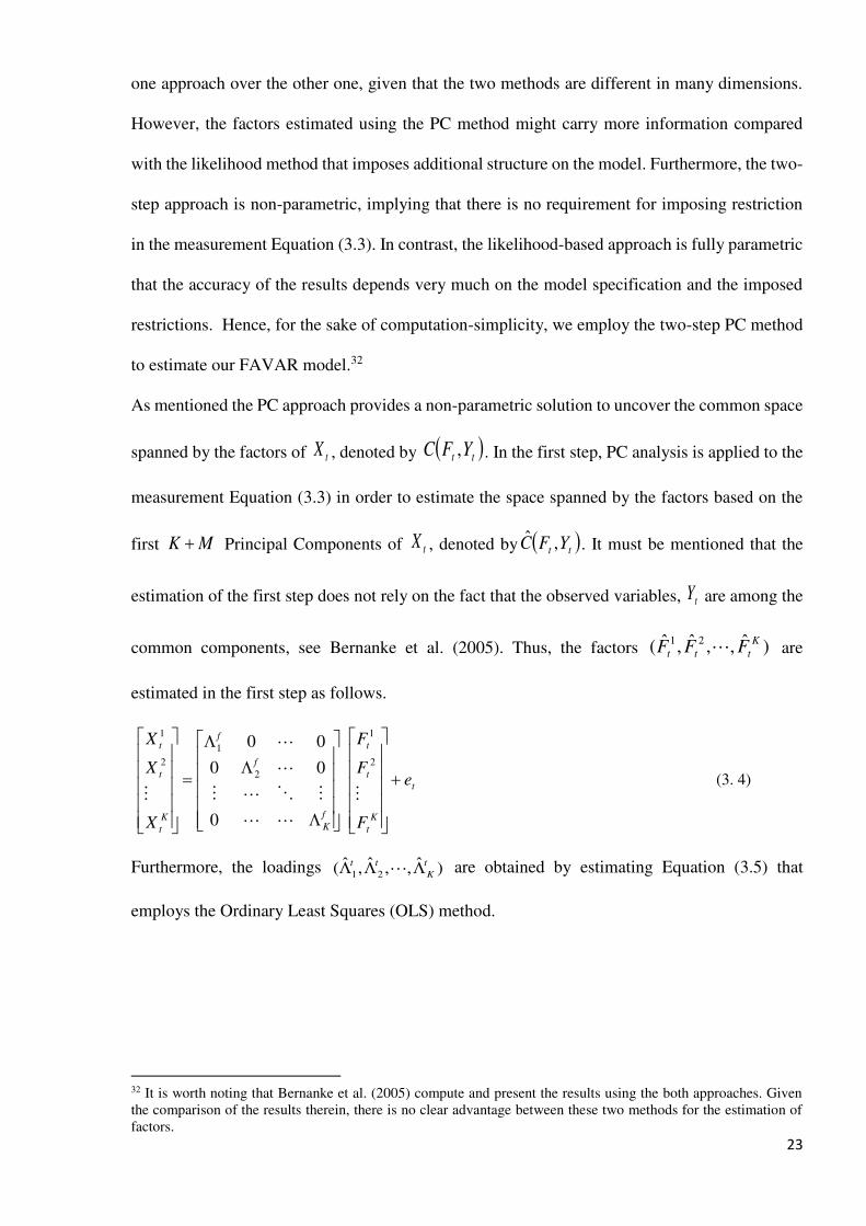
As mentioned the PC approach provides a non-parametric solution to uncover the common space

spanned by the factors of tX , denoted by tt YFC , . In the first step, PC analysis is applied to the

measurement Equation (3.3) in order to estimate the space spanned by the factors based on the

first MK Principal Components of tX , denoted by tt YFC ,ˆ . It must be mentioned that the

estimation of the first step does not rely on the fact that the observed variables, tY are among the

common components, see Bernanke et al. (2005). Thus, the factors )ˆ,,ˆ,ˆ( 21 K

ttt FFF are

estimated in the first step as follows.

t

K

t

t

t

f

K

f

f

K

t

t

t

e

F

F

F

X

X

X

2

1

2

1

2

1

0

00

00

(3. 4)

Furthermore, the loadings )ˆ,,ˆ,ˆ( 21

t

K

tt are obtained by estimating Equation (3.5) that

employs the Ordinary Least Squares (OLS) method.

32 It is worth noting that Bernanke et al. (2005) compute and present the results using the both approaches. Given the comparison of the results therein, there is no clear advantage between these two methods for the estimation of factors.

24

t

K

t

t

t

f

K

f

f

K

t

t

t

e

F

F

F

X

X

X

ˆ

ˆ

ˆ

0

00

002

1

2

1

2

1

(3. 5)

In the second step, we replace the unobserved factors in the transition Equation (3.2) by their PC

estimates, and run a standard VAR model to obtain )(ˆ L as follows.

t

t

K

t

t

t

t

K

t

t

t

e

Y

F

F

F

L

Y

F

F

F

1

1

2

1

1

1

2

1

ˆ

ˆ

ˆ

)(

ˆ

ˆ

ˆ

(3. 6)

As is mentioned earlier, computational simplicity together with allowing for some degree of

cross-correlation in the idiosyncratic error terms te , and the fact that the two-step estimation

method impose few distributional assumptions are the main advantages for this approach. One

disadvantage of the approach, however, is the presence of "generated regressors" in the second

step. As is addressed in Bernanke et al. (2005) it is possible to obtain accurate confidence

intervals on the IRFs by implementing Kilianˈ bootstrap procedure that accounts for the

uncertainty in the factor estimation.33 Following Bernanke et al. (2005) this procedure is

employed for estimation of IRFs confidence intervals.

1.3.2 The Time-Varying Parameter FAVAR Framework

The parameters of the linear FAVAR model presented earlier are time-invariant. However,

having considered structural changes in the economy induced by the conduct of different

macroeconomic policies, it is important to measure the impact of monetary policy shocks over

different points in time by allowing the parameters of the model to change over the time, see

Primiceri (2005), Del Negro and Schorfheide (2010), and Korobilis (2013).

33 As explained in Bernanke et al. (2005) and the reference therein, in theory, when N is large relative to T , the

uncertainty in the factor estimates can be ignored.

25

Parameters can vary either gradually over time following a Multivariate Autoregressive

process, or they can change abruptly as in a Markov-Switching or Structural-Breaks pattern.

Following Primiceri (2005), Koop and Korobilis (2010), and Korobilis (2013) we adopt the TVP

approach to capture structural changes in the economy within the two-step PC approach to

estimate the FAVAR model. However, the estimated factors now are allowed to drift in both the

mean and variance parameters with a random walk pattern.

Thus, to assess the effects of policy actions over the time, the parameters of the FAVAR

model now are allowed to vary over the time. Accordingly, the TVP-FAVAR version of Equation

(3.1) will take the below form.

tPtPtttt uYBYBY 11 (3. 7)

Where ],,[ '''

tttt RZFY , and tF is a )1( K vector of latent factors. Likewise, the standard VARs

],[ '

tt RZ is a vector consists of observed variables and the monetary policy tools with )1)1(( L

dimension. Also, PjB jt ,,1, are a MM matrices of coefficients, and ),0(~ Nut

where is a MM full covariance matrix for each Tt ,,1 , with 1 LKM .

Comparable with the FAVAR model, a general specification for the TVP-FAVAR can be written

as follows.

t

t

t

t

t

tu

Y

FL

Y

F

1

1)( (3. 8)

te

tY

yitt

Ffit

X it (3. 9)

Where Equations (3.8) and (3.9) represent the state and measurement equation, respectively.

Each of the Ni ,,1 original observed series itX is linked to the factors, the other observed

variables,'

tZ , and the monetary policy tool, tR , by a factor analysis regression with cross auto-

correlated errors and stochastic volatility defined as follows;

itt

R

it

Z

it

F

iit uRZFX ˆˆˆ (3. 10)

26

And

itqitiqitiit uuu 11 (3. 11)

Where RZ ˆ,ˆ are )1( N , and F̂ is )( KN . The errors are ))exp(,0(~ itit hN , and are

assumed to be uncorrelated with the factors. As is explained in Korobilis (2013), working with

uncorrelated errors required that Equation (3.10) to be transformed as formulated in Equation

(3.12);

ttt

R

t

Z

t

F

t XLRZFX )( (3. 12)

Where ))(,),(()( 1LLdiagL

n , qiqil

iLLL )( ,and

f

n

iLI ˆ))(( for

RZFj ,, . Also, ),0(~ tt HN where ))exp(,),(exp( 1 ntt hhdiagH , and the individual log-

volatilities evolves as a drift-less random walk as follows;

h

titit hh 1 (3. 13)

Where ),0(~ t

h

t N . As has been discussed in Korobilis (2013), in attempt to parameterize the

large covariance matrices related to Equation (3.7) which presents a VAR system on the factors

and observable variables, '

tZ and tR , with drifting coefficients and stochastic volatility, it is

possible to decompose the FAVAR error covariance matrix in the following form;

ttttt AA (3. 14)

Where tA is a unit lower triangular matrix, and t is the diagonal matrix.

1

0

1

001

),1(,1

,21

tmmtm

t

tA

,

tn

t

t

t

,

,2

,1

00

0

0

00

To proceed with parameter estimation, let ))(,,)(( 1 pttt BvecBvecB be a vector

consists of all the parameters of the Equation (3.7). In addition, ),,( '

),1(

'

1 tjjjt aa where

mj ,,1 be the vector of non-zero and non-one elements of the matrix tA , and

27

)log,,(loglog ''

1 nttt be the vector of the diagonal elements of the matrix

t . Assuming

that all these three drifting parameters, 'log,, ttB follow random walks, for each period the

innovations of the parameters can be formulated as follows;

B

t

B

ttt JBB 1 (3. 15)

tttt J 1 (3. 16)

tttt J 1loglog (3. 17)

Where ),0(~ QNt

are independent innovation vectors, Q are innovation covariance

matrices associated with each of the parameters vectors, and }log,,{ tttt B .34

Furthermore, the random variables tJ are defined to take only two values: one and zero at each

period t. This property allows that the state errors be a mixture of a normal component with

covariance Q , and a second component that places all probability point mass at zero, see

Korobilis (2013). The random variables tJ are updated and determined based on the data

likelihood allowing them to take either the specification of constant-parameters as

TtJ t ,,1,0 , or Time-Varying Parameters as TtJ t ,,1,1 .

The unobserved variables and the model parameters can be estimated in one-step by employing

the Markov Chain Monte Carlo (MCMC) approach. However, as has been discussed in Koop

and Korobilis (2010), and Korobilis (2013) the MCMC method makes the estimation procedure

unnecessarily complicated for computing the latent factors compared with the two-steps PC

estimator method. As explained earlier it is simpler to obtain the factors from PC method and

employ them in a TVP-FAVAR model allowing that the drifting mean and variance parameters

to follow a random walk. This assumption, which is based on a standard state-space method,

simplifies the estimation procedure, see Koop and Korobilis (2010), and Korobilis (2013). Thus,

likewise FAVAR model, the PC method is applied to estimate the factors, while the MCMC

34 A detailed discussion can be found in Primiceri (2005) and Korobilis (2013).

28

simulation method is adopted to estimate the Time-Varying Parameters in Equations (3.15) to

(3.17).

The next section proceeds to estimate a FAVAR model with Constant-Parameters followed

by estimating a TVP-FAVAR model with monetary and fiscal policy variables. These two

versions of the FAVAR model are employed for monetary and fiscal policy analysis.

1.4 Empirical Results

This section presents the empirical findings. As mentioned earlier the study pursues two

objectives. First, examining the impact of monetary and fiscal policy interactions and

investigating whether the impact is changes over the time. Second, identifying the extent to

which the transmission of monetary policy is affected by US fiscal policy. For this purpose, we

extend the Constant-Parameter FAVAR and the TVP-FAVAR models presented in Bernanke et

al. (2005), and Korobilis (2013) in two regards.

First, we account for fiscal policy to examine the impact of fiscal policy on monetary policy

and its effect on the economy. Second, we incorporate the period after the financial crisis in our

analysis. Prior to presenting the results, the model specification together with the dataset is

explained followed by the identification approach. Then, the section proceeds to estimate the

linear and TVP-FAVAR models.

1.4.1 Model Specification

Given this paper motivation, we estimate two different models namely the simple model and the

fiscal-augmented model under Constant-Parameter FAVAR and TVP-FAVAR specifications.

The simple model is specified as it excludes fiscal-related information while the fiscal stance is

captured in the fiscal-augmented model.

The model is estimated over the 1959:Q1-2013:Q2 sample. The choice of the sample is

driven by the idea to assess the conduct of monetary policy over four representative periods:

1975:Q1, 1981:Q3, 1996:Q1, and 2006:Q2 as representative of the chairmanships of Burns,

Volcker, Greenspan, and Bernanke respectively. The study involves dataset consists of 195 US

29

macroeconomic time series collected from the St Louis Fed FRED database.35 Following common

practice in this literature, all variables are transformed to be stationary using a number of methods

including the computation of their first difference.36 Appendix 3.A provide a detailed explanation

of the procedure. All the time series are seasonally adjusted were this is applicable.37

Consistent with the Factor Modelling literature, macroeconomic time series is selected to

represent the following categories: Real Output and Income, Employment and Hours,

Consumption, Housing Starts and Sales, Real Inventories and Orders Indices, Exchange Rates,

Interest Rates, Money and Credit Quantity Aggregates, Price Indices, Average Hourly Earnings,

the Fiscal Stance, and Consumers Expectations, see Appendix 3.A. As regards determining the

number of factors involved in the FAVAR model, we follow Bernanke et al. (2005) approach that

is based on the sensitivity of the results to the alternative number of factors. As have been reported

in Bernanke et al. (2005), and Korobilis (2013) the qualitative results are not altered when the

number of factors increased from three to five factors. We also estimate our specified Constant-

Parameter FAVAR model with three and five factors. As the obtained results appear to have fairly

the same qualitative pattern, both the linear and TVP-FAVAR models are constructed with three

factors to maintain parsimony.38

The lag length of the state Equations (3.2) and (3.8) is another important specification to be

determined. The lag lengths are selected in the VAR literature based on statistical criterion such

as AIC, BIC, or SIC. In the FAVAR literature, however, no specific criterion is used, to our

knowledge. Bernanke et al. (2005) employ 13 lags in order to allow sufficient dynamics in their

model. On the other hand, Stock and Watson (2005) estimate a 2-lag model. We follow Bernanke

et al. (2005) approach and construct our model with 13 lags.

35 A detailed description of database is provided in Appendix 3.A section. 36 We follow Bernanke et al. (2005), Stock and Watson (2005), and Korobilis (2013) procedure to ensure stationary

properties of the time series. 37 The time series are seasonally adjusted using the Demetra+ package developed by Eurostat. To seasonally adjust the time series, the TRAMOSEATS method has been employed. This method can be divided into two main parts: a pre-adjustment step, which removes the deterministic component of the series by means of a regression model with Arima noises and the decomposition part itself. See Grudkowska (2013) for a detailed explanation. 38 As discussed in Bernanke et al. (2005) increasing the number of factors does not appear to improve the results.

30

With reference to the observable variables required to be isolated in the VAR part,tY , our

VAR includes inflation, Industrial Production growth, and the Federal Funds rate.39 Thus, our

FAVAR is a trivariate VAR augmented with three unobservable factors, tF , which are extracted

from the large set of time series macroeconomic variables as is addressed in Appendix 3.A, and

includes fiscal variables. We use the PC approach to extract the factors. The use of PC method

ensures identification of the model since it normalizes all factors to have zero mean and unit

variance, see Korobilis (2013).

1.4.2 Monetary Policy Shock Identification

There are a number of approaches for identification of monetary policy shocks in the VAR

literature. These includes recursive identification approach, long-run restrictions, or structural

VAR procedures that can also be implemented in the FAVAR framework, see Bernanke et al.

(2005). The recursive identification is standard in much of the VAR literature and

straightforward to apply.40 On the other hand, the other competing identification approaches

would require restrictions to be imposed on the factors to identify them as specific economic

concepts.41

Thus, we follow Bernanke et al. (2005) and focus upon a recursive approach to identify

monetary policy shock. This approach assumes that the monetary authority reacts simultaneously

to macroeconomic shocks. However, macroeconomic variables react to monetary impulses with

lags. Thus, monetary policy actions influence inflation and Industrial Production growth with at

39 We followed Bernanke et al. (2005) approach to put Industrial Production growth as observable variable in the

VAR to proxy output. As Bernanke et al. (2005) explain, "Output in the theoretical model may correspond more

closely to a latent measure of economic activity than to a specific data series such as real GDP". Thus, we include

GDP as a time series in our information to extract the unobserved factors. We, then, present the IRFs of GDP to the policy shock within the FAVAR model. 40 See Christiano et al. (1999), Favero and Monacelli (2003), Bernanke et al. (2005), Primiceri (2005), Koop and Korobilis (2010), and Korobilis (2013) among others. 41 As is addressed in Bernanke et al. (2005) implementing long-run restrictions requires these restrictions to be identified separately from the other factors. One potential way to achieve this is extracting Principal Components from blocks of data corresponding to different dimensions of the economy. For example, real-activity measure is possible to be considered as is obtained solely from the output gap. This identification approach is explored in Korobilis (2013) together with the recursive approach. Comparing the IRFs results obtained from recursive identification approach and those from the block factors in Korobilis (2013), it appears that there is no substantial difference between responses.

31

least one period of lag, while the time lag for interest rate is zero by ordering it last in the VAR

part.42 Furthermore, it treats inflation as predetermined, which is consistent with estimating a

Taylor Rule that regresses the nominal interest rate on inflation, see Bernanke et al. (2005), and

Chung et al. (2007).

The standard recursive approach implies that the Fed Funds rate, tR , as monetary policy

instrument is ordered last and its innovations are treated as the policy shocks while the

unobservable factors and variables respond to the policy shock with time lags which is a quarter

in this study. As discussed in Bernanke et al. (2005) two blocks of information variables can be

defined: (i) the slow-moving variables, and (ii) the fast-moving variables. The slow-moving block

of variables is assumed that respond to monetary policy shocks with a quarter lag. In contrast, the

fast-moving block of variables reacts instantly to the policy shocks.43

To estimate the FAVAR model using the two-step PC approach, the first step ),(ˆtt YFC must be

calculated. Given that tY is not explicitly imposed as a common component in the first step, it is

possible that any of the linear combinations of ),(ˆtt YFC involves the policy instrument, tR . Thus,

the dependency of ),(ˆtt YFC on tR must be eliminated in order that the policy shock recursive

identification to be valid, see Bernanke et al. (2005). One potential solution here is to estimate the

coefficients of ),(ˆtt YFC from a multiple regression as follows.

ttRtCtt eRbFCbYFC )(*ˆ),(ˆ* (3. 18)

Where )(*ˆtFC is an estimate of all the common components subtracted tR . Then, )(*ˆ

tFC can

be obtained by extracting PC from the slow-moving block of variables which cannot be affected

42 As explained in Primiceri (2005) ordering interest rates last in the VAR is not simply an ordering issue, but an identification condition that is essential for isolating monetary policy shock. 43 The slow-moving block of variables includes Real Output and Income, Employment and Hours, Consumption, Price Indices, Average Hourly Earnings, the Fiscal Stance, and Consumers Expectations. The fast-moving block of variables includes Housing Starts and Sales, Real Inventories and Orders Indices, Exchange Rates, Interest Rates, and Money and Credit Quantity Aggregates, see Appendix 3.A for details.

32

instantly by tR . Now, tF̂ can be constructed as tRtt RbYFC ˆ),(ˆ , and a VAR between tF̂ and tY

will be estimated which is identified recursively, and the monetary policy instrument, tR , is

ordered last.44

Now we proceed to the TVP-FAVAR model identification. To study the way that monetary policy

interactions may evolve over the time, the parameters of the FAVAR are allowed to vary through

time. The sources of time variation are both coefficients and the variance-covariance matrix of

the shocks. This way, it is possible to distinguish between the exogenous shocks and changes in

the transmission mechanism, see Primiceri (2005). As is discussed in Koop and Korobilis (2010),

and Korobilis (2013) obtaining sensible results from TVP-FAVAR model requires the imposing

of restrictions to allow only particular parameters to vary over time.

A general specification for TVP-FAVAR model can be acquired using these following restrictions

imposed to the measurement and the state equation of the TVP-FAVAR in the form of Equations

(3.19) and (3.20) respectively. Note that tX represents all the information in time series using to

extract the unobservable factors, tF represents the factors, and tR represents the monetary policy

instrument.

ittittitoitit RFX (3. 19)

F

t

pt

pt

pt

t

t

t

t

t

R

F

R

F

R

F̂ˆˆ

1

1

1

(3. 20)

As regards the estimation of Equations (3.19) and (3.20), the following issues must be taken

into account.

1. Each innovation term, it , in the measurement equation follows an univariate stochastic

volatility process,

2. F

t

F

t ˆ)ˆ(var has a multivariate stochastic volatility process,

44 A detailed explanation of the identification using the PC approach can be found in Bernanke et al. (2005).

33

3. ptt ˆ,,ˆ1 Which are the coefficients of the state equation are allowed to vary in

accordance with random walk model.45

Following Primiceri (2005), Koop and Korobilis (2010), and Korobilis (2013) the simulations is

carried based on 10,000 iterations of the Gibbs sampler, discarding the first 2000 for

convergence. Given the dimension of the model and the presence of TVP, some shrinkage in the

model is required. One potential approach to provide shrinkage in the model is to employ the

prior. This study follows Koop and Korobilis (2010) and employs the Minnesota prior that is a

standard one in the VAR literature. The key property of this prior is that the own lags of each

variable is weighted more than lags of other variables.46

Having established the identification of monetary policy shock, the next section presents the IRFs

for both the linear and TVP-FAVAR models.

3.4.3 The FAVAR Model Specification Results to Monetary Shock

This section presents the empirical results for the Constant-Parameter FAVAR model estimated

by the two-step Principal Components approach. The objective is to investigate the impact of

monetary and fiscal policy interactions on the US economy. In particular, it aims to examine the

way in which monetary policy transmission mechanism may be influenced by the fiscal stance.

Two FAVAR models are specified for estimation: a simple FAVAR model, and a fiscal-

augmented FAVAR model. The simple model is based on the Bernanke et al. (2005) FAVAR

model that excludes the fiscal variables. It is instructive to compare the results obtained from the

simple FAVAR model with the fiscal-augmented one to understand the potential impact of the

fiscal stance on the economy.

Figure 3.2 presents the Impulse Response Functions (IRF) to a recursively identified

contractionary monetary policy shock. The IRFs are generated within the simple FAVAR model

45 As explained in Koop and Korobilis (2010), it is difficult to estimate time variation of coefficients in both the measurement and the state equation in absence of strong prior information. 46 A more detailed discussion of this choice compared with the alternative prior specification can be found in Koop and Korobilis (2010), and Korobilis (2013).

34

with three unobserved factors and three observed variables in the VAR. The three observed

variables in the VAR section include Inflation, Industrial Production growth, and the nominal

Federal Funds rate.47 It is expected that a monetary contraction shall induce small and transitory

effects on interest rates with a rather large and persistent impact on output and prices, see Barth

and Ramey (2002) and Eichenbaum (1992). As can be seen in the graph, inflation is unresponsive

first, and then slightly falls in response to a monetary contraction although this is statistically

insignificant. There is no evidence of the price puzzle. Moreover, Industrial Production growth

declines in response to the shock that is consistent with the conventional view in the literature.

However, the response of output appear to be statistically insignificant.

The FAVAR model provides us with a broad set of responses to the monetary shocks, to

which we turn now. According to IRFs plotted in Figure 3.2, the responses of the other

macroeconomic variables in the FAVAR are generally consistent with economic intuition. A

monetary contraction reduces the growth rate of real activity measures including GDP, new

orders index, new housing starts, and average hourly earnings. Unemployment also increases.

The response of these real activity indicators appears to be statistically significant. In addition,

both durable and non-durable consumption fall in response to the shock that appears to be

statistically significant.48 This can be explained through a negative wealth effect. A rise in Fed

Funds rates would induce asset prices to fall as equities would be substituted by bonds, see

Mishkin (1995). This, in turns, would generate a negative wealth effect leading to a reduction in

private expenditure including consumption and new housing starts.

Moreover, the response of money aggregate measures such as monetary base, money

supply, and loans is consistent with the intuition: all appear to decline in response to a monetary

contraction as the opportunity cost of holding money increases. As Figure 3.2 shows, the

responses of monetary aggregate measures appear to be statistically significant.

47 We follow Bernanke et al. (2005), Primeceri (2005), and Korobilis (2013) and construct both the FAVAR and TVP-FAVAR models using nominal variables. 48 Fuhrer and Rudebusch (2004) point out that expenditure on durable goods is the most interest-sensitive components of aggregate consumption.

35

36

Figure 3.2.The IRFs to a US Monetary Contraction within the Simple FAVAR

Note: This Figure illustrates IRFs to a contractionary monetary shock from a FAVAR with constant parameters. The VAR part of the model includes the Federal Funds rate, Industrial Production growth, and Inflation on top panel. The IRFs of other key variables in the monetary transmission mechanism is estimated based on three unobserved factors. The Impulse Responses together with their confidence intervals (10th, 50th, and 90th) are generated based on Bernanke et al. (2005) FAVAR model specification corresponds to a one standard deviation increase to the Federal Fund Rate. The FAVAR model is estimated using the Two-Step Principal Components approach from Bernanke et al. (2005) over the 1959:Q1-2013:Q2 sample.

We are now looking at the monetary transmission in which monetary policy influences the

economy. As regards the impact of the policy upon the exchange rate, it is expected that higher

interest rates appreciate the domestic currency and cause asset prices to fall. As is visible in

Figure 3.2, the US exchange rate to Japanese Yen remains unresponsive up to 12 quarters and

falls after that. An increase in the Federal Funds rate, also, induces the long-term interest rate to

increase which remains significant up to 9 quarters. Furthermore, as the opportunity cost of

holding money increasing, it would induce bank reserves to fall, see Mishkin (1995). Confronting

the IRFs results presented in Figure 3.2 with the literature on the monetary transmission, it

appears that responses are consistent and excluding inflation, industrial production growth, and

the exchange rate, the response of others remains statistically significant for quite some time.

37

Comparing the results from the simple FAVAR, which excludes fiscal variables in the factors,

with those of Bernanke et al. (2005) a few notable features emerge.49 Unlike Bernanke et al.

(2005) there is no evidence of the price puzzle in our simple FAVAR model specification,

however, inflation stays unresponsive to the policy shock for half of the period and then slightly

falls.50 This is a dissatisfactory aspect of our most basic FAVAR model, since it is generally

believed that monetary policy can influence inflation. It appears that increasing the time span

under study and involving extra information for extracting factors could contribute to

disappearance of the price puzzle. According to Sims (1992) if the addition of extra information

mitigates the price puzzle, it can be concluded that the new time series contain useful information

for the economy. Moreover, the response of average hourly earnings is counterintuitive in

Bernanke et al. (2005), that is the same pattern as inflation in response to monetary contraction.

However, our results seem to be reasonable as it falls in response to the policy shock that

statistically is significant for quite large interval, see Figure 3.2.

Having presented the main results from the simple FAVAR model, now we proceed to consider

the impact of fiscal policy on the economy and the monetary transmission mechanism. Figure 3.3

presents the IRFs results of the benchmark linear FAVAR model augmented with the fiscal

variables in the factors.51 We consider the case of a contractionary monetary policy shock. In

general, as the IRFs suggest including the fiscal stance influence the responses and the

transmission mechanism. Similar to the simple FAVAR model specification, Industrial

Production growth falls in the fiscal-augmented model in response to a monetary contraction.

49 Note that the simple FAVAR models is estimated based on information from 165 macroeconomic time series representing economic activity except the fiscal stance, while those presented in Bernanke et al. (2005) relies on 120 macroeconomic time series. 50 The results obtained from a FAVAR model in Bernanke et al. (2005) display the price puzzle which disappears after a short while. 51 In order to study the impact of monetary policy shock, the fiscal-augmented FAVAR model, in both linear and non-linear approaches, is constructed by including the fiscal-stance related variables in Xt to estimate the factors as

Appendix 3.A details. The VAR part of the model,Yt , stays the same as the simple specification that includes the

Federal Funds rate, Inflation, and Industrial Production growth. Given that we employ IRF results and not the GIRFs or OIFs, by inserting both fiscal and monetary policy shocks instruments into the VAR, orthogonality would be an issue to obtain reasonable results. Note that both the GIRFs and OIFs guarantee that various imposed shocks to the system are uncorrelated. Paper 4 explores this idea further.

38

However, comparing the response of inflation from the simple model with the fiscal-FAVAR, it

is evident that inflation increases in the latter model while it remains unresponsive and eventually

falls within the simple model. It worthy to note that the response of both Industrial Production

growth and inflation remains statistically insignificant.

Taking account of fiscal variables may explain the response of inflation within the fiscal-

augmented FAVAR model. In the presence of large and persistent government debt, the monetary

authorities are forced to increase the money supply in order to accommodate the growth in money

demand induced by the debt, see Bradley (1984). The mechanism works as follows. A monetary

contraction would force the fiscal authority to issue new bonds to finance the increase in

government debt induced by higher interest rates. This would increase the demand for money as

the demand for bonds increase. This can lead to an increase in inflation. In addition, the issuance

of new bonds and the higher interest rates can generate positive wealth effects, see Canzoneri et

al. (2011). This positive wealth effect can induce aggregate demand to increase through private

consumption leading to a raise in inflation.

Turning to Figure 3.3, we can see that consumption increases and then falls in response to

monetary contraction. Consumersˈexpectations also rises on impact, and then gradually returns

to zero. The increase in consumption, both durable and non-durable, can suggest that this policy-

induced increase in the interest rates generates a positive wealth effect contributing to an increase

in inflation. Thus, it appeared that involving fiscal policy within linear fiscal-augmented can

influence the response of inflation to a monetary policy shock compared with the more limited

model FAVAR.

With reference to a fall in Industrial Production growth and a rise in inflation associated with a

monetary contraction, these results might be in line with the cost-channel interpretation of the

price puzzle as proposed by Barth and Ramey (2002). That is a policy-induced increase in the

interest rate causes the unit cost of production to increase leading to a rise in prices and a fall in

output when capital is an important component of output.

39

Figure 3.3. The IRFs to a US Monetary Contraction within the Fiscal-Augmented FAVAR

Note: This Figure illustrates IRFs to a contractionary monetary shock within a constant parameter FAVAR augmented with fiscal variables. The VAR part of the model includes the Federal Funds rate, Industrial

Production growth, and Inflation on top panel. The IRFs of other key variables in the monetary transmission mechanism is estimated based on three unobserved factors. The Impulse Responses together with their confidence intervals (10th, 50th, and 90th) are generated based on Bernanke et al. (2005) FAVAR model specification corresponds to a one standard deviation increase to the Federal Fund Rate. The FAVAR model is estimated using the Two-Step Principal Components approach from Bernanke et al. (2005) over the 1959:Q1-2013:Q2 sample.

Another clear distinction between the two FAVAR model specifications is related to the measure

of monetary aggregate. As illustrated in Figure 3.3, both monetary base and money supply

increase in response to the policy shock in the fiscal-augmented model while both fall in the

simple FAVAR. This finding is consistent with Bradley (1984) explanation of the impact of debt

on monetary aggregate and prices consequently, which can be referred to as the debt monetizing.

Within the simple FAVAR, there is a fall in other real activity measures, i.e. GDP,

unemployment, the average hourly earnings, new housing starts, and new orders index, in

response to monetary contraction. The fiscal-FAVAR also indicates that real activity falls. As

regards the fiscal variables, Figure 3.3 indicates that total government expenditure and the interest

payments on the public debt increase in response to a monetary contraction, while government

40

debt-to-GDP is particularly unchanged. However, the fiscal variables responses are statistically

insignificant.

To summarize, the IRFs so far suggests that a monetary contraction reduces output growth

and real activity measures within a linear FAVAR, irrespective of whether the fiscal stance is

included or not. However, while inflation falls within the simple model, it increases in response

to the policy shock in the fiscal-augmented model. It worthy of note, though, that the responses

of Industrial Production growth and inflation are statistically insignificant for the both model

specifications. The insignificant results may suggest that the impact of monetary policy shocks

are time varying, given the existing literature on monetary and fiscal policy regime changes, see

Favero and Monacelli (2003), and Davig and Leeper (2007, 2012). This can also be seen in the

results presented in Bernanke et al. (2005) as the response of inflation and Industrial Production

growth are not statistically significant.

To study the way that monetary and fiscal policy interactions may evolve over the time, the next

section presents the results from a TVP-FAVAR model.

3.4.4 The TVP-FAVAR Model Specification Results to Monetary Shock

Several studies find evidence supporting that macroeconomic policy in the United States changed

regimes, see Favero and Monacelli (2003), Chung et al. (2007), and Davig and Leeper (2007,

2011). Given this paper motivation, we examine the potential influence of changes in monetary

and fiscal policy performance on the economy, and the transmission mechanism of policy

shocks. Likewise the linear FAVAR model, the impact of the fiscal variables on the monetary

policy over the time is examined within both the simple and the fiscal-augmented TVP-FAVAR

model. The model specification and identification of the shocks is the same as explained in the

linear FAVAR model.

Figures 3.4 to 3.11 present the results for both the simple and the fiscal-augmented TVP-

FAVAR models. The monetary policy shock is assumed as non-systematic. It means that the

policy shock can captures policy mistakes and movements in the Federal Funds rate and not the

41

changes in the structure of the economy, see Primiceri (2005), and Korobilis (2013). The

posterior mean estimates of the standard errors for the three unobserved factors and the three

observable variables in the VAR are plotted in Figures 3.4 to 3.7. The standard deviation values

are the square roots of the main-diagonal elements of the matrix t , for all t . Hence, higher

standard deviation of monetary policy shocks is associated with higher policy mistakes, see

Korobilis (2013).

As Figures 3.4 and 3.5 illustrate, including the fiscal stance to the TVP-FAVAR model

decreases the posterior mean of the standard deviations for the estimated factors. In comparison

with those presented in Korobilis (2013), that is estimated under Bernanke et al. (2005)

identification, it appears that the mean values of the standard deviations in our results within both

the simple and the fiscal-augmented model are much lower. This decline in the standard

deviations of the residuals may imply that including the fiscal stance and extending the sample

have influence on reducing policy errors, specifically after the 1980s.

As can be observed in Figures 3.6 and 3.7, the standard deviations of the residuals of the

observable variables in the VAR decrease when fiscal variables are included in the model

compared with the simple TVP-FAVAR. As regards with the posterior mean of the standard

deviations of inflation, mainly two episodes within the fiscal-augmented model can be identified:

one before 1975 that the mean values ranging around of 0.8, and another one after 1981 that the

mean values falling around of 0.4.

42

Figure 3.4. Posterior Mean of the SD of Residuals of the Factors within the Simple TVP-

FAVAR

Note: Figure presents the Time-Varying Standard Deviations (SD) of the errors within the simple TVP-FAVAR model with Three Unobserved Factors over the 1959:Q1-2013:Q2 sample. The FAVAR part of the model is estimated using the Two-Step Principal Components method based on Bernanke et al. (2005) identification approach.

Figure 3.5. Posterior Mean of the SD of Residuals of the Factors within the Fiscal-

Augmented TVP-FAVAR

Note: Figure presents the Time-Varying Standard Deviations (SD) of errors within the fiscal-augmented TVP-FAVAR model with Three Unobserved Factors over the 1959:Q1-2013:Q2 sample. The FAVAR part of the model is estimated using the Two-Step Principal Components method based on Bernanke et al. (2005) identification approach.

43

Figure 3.6. Posterior Mean of the SD of Residuals for the Observable Variables within the

Simple TVP-FAVAR

Note: Figure presents the Time-Varying Standard Deviations (SD) of errors within the simple TVP-FAVAR model with Three Unobserved Factors over the 1959:Q1-2013:Q2 sample. The FAVAR part of the model is estimated using the Two-Step Principal Components method based on Bernanke et al. (2005) identification approach.

Figure 3.7. Posterior Mean of the SD of Residuals for the Observable Variables within the

Fiscal-Augmented TVP-FAVAR

Note: Figure presents the Time-Varying Standard Deviations (SD) of errors within the fiscal-augmented TVP-FAVAR model with Three Unobserved Factors over the 1959:Q1-2013:Q2 sample. The FAVAR part of the model is estimated using the Two-Step Principal Components method based on Bernanke et al. (2005) identification approach.

44

There is an overlap between the higher mean value and the periods that have been known

as the active episodes of fiscal policy and vice versa. As is visible in the fiscal-augmented model,

Figure 3.7, the highest peak in volatility of residual for inflation occurred in 1975. This finding

is reported by Primiceri (2005), and Korobilis (2013). They relate these peaks in volatility to the

Great inflation, e.g. the shock in price of oil in 1974, and the Monetarist experiment by the

increase of interest rates in 1981. The interval is also associated with a change in the conduct of

monetary policy targeting bank reserves, i.e. monetary aggregate, instead of interest rates that

lead to a rapid increase in interest rates. Then, the second peak, which appears to be quite modest,

is associated with the financial crisis in 2008. Having considered monetary and fiscal policy

regimes as identified in Favero and Monacelli (2003), and Davig and Leeper (2007, 2011) we

can see that the both peaks are associated with an active fiscal policy coordinated with a passive

monetary policy.

As regards the residuals of Industrial Production growth, the highest peak in volatility for

both model specifications is occurred in 1975. However, the mean value of residuals appears to

be higher, around of 2, for the simple model compared with the fiscal-augmented model, around

of 1.5. Furthermore, as can be observed in Figures 3.6 and 3.7, the volatility of the standard

deviation of residuals for the Federal Funds rate reaches its highest value at 1981 that is consistent

with the results presented in Primiceri (2005), and Korobilis (2013) that is referred as the

Monetarist Experiment in the literature. In addition, as is visible in the graph, the mean value of

the residuals falls in the model includes fiscal variables.

The interval between 1985 and 2007 demonstrates a very modest pattern for the both

estimated factors and indicator variables within both the simple and the fiscal-augmented model.

This period is known in the literature as the Great Moderation associated with an active monetary

policy and a passive fiscal policy regimes. This suggests that active monetary policy, when the

45

nominal interest rate responds aggressively to inflation, in coordination with a passive fiscal

policy may attribute to a lower volatility in inflation and output.52

Having compared the standard deviations of the errors for both the simple and the fiscal-

augmented models, it appears that the fiscal stance contributes to decreasing the volatility and

the posterior mean of the responses to the monetary policy shock. The occurrence is more visible

for residuals of inflation matched with an active fiscal policy and a passive monetary policy

regimes. This suggests that involving the fiscal stance variables may contain important

information to explain the volatility of inflation and may influence the monetary transmission

mechanism.

We now compare IRFs of the three observable variables in the VAR part to the identified

monetary contraction shock from the simple model with the fiscal-augmented one as presented

in Figures 3.8 and 3.9. The selected sub-samples are 1975:Q1, 1981:Q3, 1996:Q1, and 2006:Q2.

These represent the chairmanships of Burns, Volcker, Greenspan, and Bernanke respectively.

These different dates allow us to capture the transmission of monetary shocks under different

macroeconomic policy regimes and business cycles phases.53

Before discussing the results, it is useful to specify monetary and fiscal policy regime at the

time when we impose policy shocks. Table 3.3 illustrate our policy shocks in terms of whether

monetary and fiscal policy are active or passive. We follow Favero and Monacelli (2003), and

Davig and Leeper (2007, 2011) to specify these different macroeconomic policy regimes.

52 Primiceri (2005) mentions that a Taylor-type Rule, that the Federal Funds rate responds to inflation strongly, may better approximate US monetary policy over the Great Moderation. 53 The 1975:Q1 represents a NBER business cycle trough date; 1981:Q3 is a NBER business cycle peak date, 1996:Q1 represents both NBER trough and peak dates, i.e. 1991:Q1: trough and 2001Q1: peak, and 2006:Q2 represents both NBER peak and trough, i.e. 2007:Q4: peak, and 2009:Q2: trough. The detailed historical record of US business cycles can be found in NBER US Business Cycle Expansions and Contractions.

46

Table 3.1. US Macroeconomic Policy Regimes Burns Volcker Greenspan Bernanke

1975 1981 1996 2006

Monetary Policy Passive Active Active Passive

Fiscal Policy Active Active Passive Active

Note: This Table reports different macroeconomic policy regimes. Different fiscal policy regimes are based on Favero and Monacelli (2003), and Davig and Leeper (2007, 2011). Monetary policy regimes are based on those reported in Davig and Leeper (2007, 2011).

It is expected that a contractionary monetary shock cause both inflation and Industrial Production

growth to decrease. Figure 3.8 shows that inflation declines within the simple TVP-FAVAR

model over the four representative periods. This is as expected. This is also consistent with the

results presented in Korobilis (2013) using the same identification as in Bernanke et al. (2005)

over the period 1981:Q3 and 1996:Q1.54 Moreover, Industrial Production growth falls in response

to a monetary contraction within the simple TVP-FAVAR model. The response for both inflation

and Industrial Production growth appears to be statistically insignificant which quickly returns

to zero, see Figure 3.8.

Figure 3.9 gives the TVP-FAVAR results with fiscal policy. In contrast to the simple model, a

monetary shock now increases inflation for 1975:Q1, 1981:Q3 and very marginally 1996:Q1.

Inflation again falls with a shock in 2006:Q2. As Table 3.3 illustrates, fiscal policy has been

active during the administration of Burns and Volcker. Then we can see that fiscal policy

switched to be passive in Greenspanˈs Chairmanship. It again turned to be active during the

administration of Bernanke. However, monetary policy was passive in the Burnsˈs administration

and turned to be active over both the Volcker and Greenspan period. Then it switched to passive

in Bernankeˈs administration.

54 Note that the results presented in Korobilis (2013) show the occurrence of the price puzzle over the 1975:Q1. His work, however, does not cover the 2006:Q2 period and is constructed upon 143 US macroeconomic time series.

47

Figure 3.8. IRFs of the Observable Variables within the Simple TVP-FAVAR

Note: The Figure shows IRFs for monetary contraction. The Impulse Responses (10th, 50th, and 90th percentiles) are generated within the simple TVP-FAVAR model with Three Unobserved Factors corresponds to a one standard deviations increase to the Federal Funds rate. The Impulse Responses are presented for four representative points in time, 1975:Q1, 1981:Q3, 1996:Q1, and 2006:Q2 as representative of the chairmanships of Burns, Volcker, Greenspan, and Bernanke respectively.

Figure 3.9. IRFs of the Observable Variables within the Fiscal-Augmented TVP-FAVAR

Note: The Figure shows IRFs for monetary contraction. The Impulse Responses (10th, 50th, and 90th percentiles) are generated within the fiscal-augmented TVP-FAVAR model with Three Unobserved Factors corresponds to a one standard deviations increase to the Federal Funds rate. The Impulse Responses are presented for four representative points in time, 1975:Q1, 1981:Q3, 1996:Q1, and 2006:Q2 as representative of the chairmanships of Burns, Volcker, Greenspan, and Bernanke respectively.

48

It appears that the price puzzle is accentuated within the periods that fiscal policy is active and

monetary policy is passive. This counter-intuitive response can be explained through a positive

wealth effect induced by a monetary contraction in the presence of an active fiscal policy. The

price puzzle then tends to reduce and disappear when fiscal policy switches to passive and

monetary policy switches to active episode.55

The mechanism can be explained as follows. An increase in the Federal Funds rate when

coordinates with an active fiscal regime, may contribute to higher interest rate payments to

bondholders. This is happening as the government debt becomes more expensive to finance. Thus,

the government must issue more liabilities. Until the price levels start to increase, the new issued

bonds create a positive wealth effect. Moreover, with sticky prices the wealth effect would stay

for some time to influence householdsˈ consumption. Thus, this positive wealth effect can shift

aggregated demand upward through increasing private consumption. This, in turns, would raise

inflation and output. Consequently, the policy outcome can be higher prices and output.

With reference to the price puzzle appeared in the fiscal-augmented model, our results are

consistent with the provided argument in Chung et al. (2007). As is argued therein, inflation

sharply increases in short-run in response to a monetary contraction. They show that the price

puzzle, which emerges in monetary VARs, can be explained as a natural outcome of periods when

monetary policy fails to obey the Taylor principle and taxes do not respond to the state of

government debt.56 Their interpretation of the price puzzle is also consistent with those of Hanson

(2004). He concludes that the price puzzle cannot be solved by the conventional method such as

adding commodity prices to the Federal Reserveˈs information set. Hanson (2004) also finds that

the puzzle is more pronounced in the 1960s and the 1970s that is identified as active fiscal policy

and passive monetary policy.

55 See Favero and Monacelli (2003), and Davig and Leeper (2007, 2011) for a detailed explanation on the estimation of active and passive monetary and fiscal policy regime changes. 56 They find empirical results from a Markov-Switching VAR model suggest that there is a positive correlation between interest rate and inflation under the non-Ricardian and non-monetarist combination case.

49

Furthermore, the response of inflation for 1975:Q1 and 1981:Q3, under active fiscal policy

regime, can validate the Sargent and Wallace (1981) view on the inflationary effects of monetary

and fiscal interactions. However, it seems that monetary policy would better account for inflation

determination for the Greenspan period, in 1996:Q1, when fiscal policy switches to passive and

monetary policy is active. A similar finding is reported in Davig and Leeper (2007,2011).

As regards Industrial Production growth, the same response as inflation within the fiscal model is

obtained suggesting that the fiscal stance can influence the responses of inflation and output

growth. The response of both inflation and Industrial Production growth is very short-lived, in

contrast to the results from the linear FAVAR, and remains statistically significant for a short

while.

The positive response of inflation and output growth to a monetary contraction are accentuated

under active fiscal policy and passive monetary policy. This is consistent with the results

presented in Chung et al. (2007), Davig and Leeper (2007, 2011), Eusepi and Preston (2011), and

Leeper and Walker (2012). As Figure 3.9 shows, the price puzzle is more pronounced in the Burns

and Volcker periods. Then, it tends to reduce in Greenspan period, and disappears in Bernanke

administration. These are consistent with Primiceri (2005) interpretation of the non-systematic

monetary policy shock. He provides evidence supporting that monetary shock become less

important in Greenspan period.

Given the descriptive statistics on the US key indicator variables over the representative sub-

samples as reported in Table 3.4, a number of features emerge that can shed light on these

unconventional responses with reference to the macroeconomic policy coordination. First, the

Federal Funds rate on average has been greater than inflation in Burns and Volcker administration.

With an increase in public debt, it implies that the new government bonds issued in coordination

with higher interest rate, due to monetary contraction, may generate positive wealth effect.57 This

wealth effect, in turns, induces private spending and inflation to increase.

57As discussed in Paper 2, a monetary contraction makes government debt more expensive to finance. This can lead the government to issue new debt. In the circumstance when government issues debt that is not fully backed by taxes,

50

Table 3.2. Mean Values for the Key Macroeconomic Indicators over the Representative

Sub-Samples

Chairmanships

Policy

Coordination

Output

Gap

Inflation The Federal

Funds Rate

Real

Rates

Government

Debt-to-GDP

Burns (1970-1978) PM- AF&PF -0.78 6.21 7.1 0.90 32.68

Volcker (1978-1987) MP&MA-FA&FP -1.48 4.97 6.79 1.82 50.22

Greenspan (1987-2006) AM-AF&PF 1.04 4.36 3.6 -0.76 59.16

Bernanke (2006-2013) MA-FA -3.47 4.30 1.35 -2.95 81.36

Overall Sample -1.17 4.96 4.71 -0.25 55.86

Note: This Table reports the mean values for the key indicator variables of the US economy under the selected representative chairmanships of the Federal Reserve. The output gap information is collected from IMF database that shows the percentage deviation between the actual GDP and its potential level. Inflation is the percentage change in the CPI. The real rates are calculated by subtracting the inflation from the Federal Funds rate. The policy coordination is reported according to monetary and fiscal policy regimes estimated by Favero and Monacelli (2003), and Davig and Leeper (2007, 2011). AM and PM abbreviate active and passive monetary policy, respectively. In addition, AF and PF abbreviate active and passive fiscal policy, respectively.

Second, during Greenspan and Bernanke periods, the Federal Funds rate has declined significantly

while inflation nearly remains close to the overall sample mean value. Thus, the real rates turn to

be negative. As reported in Table 3.4, the government debt continues to rise, in both sub-samples.

However, it seems that the low Federal Funds rate coordinated with a passive fiscal policy in

Greenspan period to be insufficient to stimulate the private spending.

This explanation is consistent with the idea discussed in Clarida et al. (2000), and Romer

and Romer (2004) stating that monetary policy has been mainly accommodative in Burns and

Volcker period.58 Thus, the positive response of inflation to monetary contraction is in accord

with the view that active fiscal policy and passive monetary policy may generate inflationary

effects. In contrast, over Greenspan administration, monetary policy switches to active

coordinated with a passive fiscal policy resulting in disappearance of the price puzzle. During

Bernanke administration, fiscal policy switches to active with a passive monetary policy in a

sense that the short-term interest rates stays irresponsive and there is no changes in inflation

either. However, as an UMP has been adopted over this period, it makes the comparison difficult.

any policy-generated increase in the interest rate would increase inflation, instead of decrease, see Cochrane (2001, 2009), Sims (2011), and Canzoneri et al. (2011). Under this circumstance, the higher interest rates will lead to the expansion of nominal government debt, particularly when interest expenses are a major part of the government budget. 58 A detailed discussion of policy actions and outcomes over the chairmanships of Burns, Volcker, and Greenspan can be found in Romer and Romer (2004), and Bae et al. (2012).

51

Figure 3.10. IRFs to a US Monetary Contraction within the Simple TVP-FAVAR

Note: The impulse responses is generated within the simple TVP-FAVAR model with Three Unobserved Factors corresponds to a one standard deviations increase to the Federal Funds rate. The VAR part of the model includes the Federal Funds rate, Industrial Production growth, and Inflation. The factors are estimated using the Two-Step Principal Components approach from Bernanke et al. (2005). Posterior medians of Impulse Responses are presented for four representative periods, 1975:Q1, 1981:Q3, 1996:Q1, and 2006:Q2 as representative of the chairmanships of Burns, Volcker, Greenspan, and Bernanke respectively.

Having discussed the impact of contractionary monetary policy on inflation and output, now we

proceed to examine the monetary transmission mechanism as displayed in Figures 3.10 and 3.11

within the simple and the fiscal TVP-FAVAR model, respectively. Figure 3.10 illustrates that the

response of other real activity measures, such as GDP, consumption, hourly earnings, new orders

index, new housing starts, and unemployment, within the simple model are generally as expected.

A monetary contraction induces the real activity to decline over Burns and Volcker periods. For

Greenspan these variables remain unresponsive to the policy shock, while during Bernanke

administration durable consumption, and GDP slightly increase in response to the shock that is

counterintuitive. The very weak response of inflation in Bernanke period, as presented in Figure

3.8, may clarify this result. As regards monetary variables, it can be seen that broad money,

money supply, and loans fall in the Burns and Volcker period, while they increase in the

52

Greenspan and Bernanke periods, respectively. The IRFs results within the simple model are

consistent with those presented in Korobilis (2013).

The IRFs results from the fiscal model, as plotted in Figure 3.11, show that real activity

measures variables increase during the Chairmanships of Burns and Volcker. This is

unconventional. These two sub-samples are associated with an active fiscal policy. We can see

the potential positive wealth channel in these two episodes as non-durable consumption increase.

When fiscal policy switches to passive while there is an active monetary policy, the monetary

contraction generates results that are more reasonable.

Figure 3.11 indicates that over Greenspan and Bernanke administration, real activity

measures shows a sharp increase on impact, and then fall. Our results are overall consistent with

the discussion in Davig and Leeper (2007, 2011), Sims (2011), and Leeper and Walker (2012)

regarding inflationary impact of a monetary contraction under an active fiscal policy and a

passive monetary policy regimes.

The same unconventional responses are obtained for monetary aggregates. As Figure 3.11

demonstrates, under active fiscal policy and passive monetary policy regimes, monetary base,

supply of money, and loans increases instead of falling. In contrast, the IRFs results of these

variables appear to be conventional in the case of a passive fiscal policy and an active monetary

policy during Greenspan and Bernanke period. These results suggest that the fiscal stance may

influence the monetary transmission mechanism. In addition, our results are consistent with

finding presented in Favero and Monacelli (2003) that fiscal policy significantly influences the

price level determination when fiscal and monetary policy appears in mismatch exactly as it

appears to happen before 1987.

53

Figure 3.11. IRFs to US Monetary Contraction within the Fiscal-Augmented TVP-FAVAR

Note: The impulse responses is generated within the fiscal-augmented TVP-FAVAR model with Three Unobserved Factors corresponds to a one standard deviations increase to the Federal Funds rate. The VAR part of the model includes the Federal Funds rate, Industrial Production growth, and Inflation. The factors are estimated using the Two-Step Principal Components approach from Bernanke et al. (2005). Posterior medians of Impulse Responses are presented for four representative periods, 1975:Q1, 1981:Q3, 1996:Q1, and 2006:Q2 as representative of the chairmanships of Burns, Volcker, Greenspan, and Bernanke respectively.

As regards the fiscal stance variables responses, monetary contraction shock induces

government debt and total government expenditures to increases as the interest payments on

government debt increase under an active fiscal policy periods: 1975:Q1 and marginally over

1981:Q3. During these periods, the Federal Funds rate has been much higher compared with the

1996:Q1 and 2006:Q2. Then, as the interest payments on debt stay unresponsive and falls, both

the debt-to-GDP ratio and total government expenditure follow the same path, see Figure 3.11.

Table 3.5 clarifies the monetary-fiscal interactions with reference to the macroeconomic policy

regimes. As can be seen in the Table, the generated wealth effect is associated with the periods

that fiscal policy is active and the growth rate of the interest expenses of public debt are positive.

It implies that a monetary contraction may contribute to the issuance of new government bonds.

This, in turns, may induce an increase in consumption through a positive wealth effect. The

impact can be traced under active fiscal policy and passive monetary policy regimes.

54

Table 3.3. The US Monetary-Fiscal Interactions and the Monetary Transmission Results

Chairmanships

Policy

Coordination

Wealth

Effects

Non-Durable

Consumption

Price Puzzle Growth Rate of

Interest Share of

Government Debt

Burns (1970-1978) PM- AF&PF YES Increase YES 1.28

Volcker (1978-1987) MP&MA-FA&FP

YES Small Increase

YES 0.19

Greenspan (1987-2006) AM-AF&PF NO Unresponsive NO -0.98

Bernanke (2006-2013) MA-FA NO Falls NO -3.89

Note: This Table reports the outcome of US monetary-fiscal interactions under the selected representative chairmanships of the Federal Reserve. The policy coordination is reported according to monetary and fiscal policy regimes estimated by Favero and Monacelli (2003), and Davig and Leeper (2007, 2011). AM and PM abbreviate active and passive monetary policy, respectively. In addition, AF and PF abbreviate active and passive fiscal policy, respectively.

Thus, the IRFs presented in Figures 3.9 and 3.11 confirm the different interpretation for the price

puzzle discussed in Chung et al. (2007). They explain that an increase in prices in response to

monetary contraction may be a normal response rather than a puzzle when fiscal policy is active

and considered in the monetary transmission mechanism.

In summary, comparing the IRFs results from the fiscal-augmented TVP-FAVAR with those from

the simple model, three features emerge. First, including the fiscal stance to examine the monetary

transmission mechanism can results in the price puzzles. Second, the price puzzle is accentuated

under an active fiscal policy and a passive monetary policy coordination. Third, a positive wealth

effects appears to contribute to increasing prices through consumption within the fiscal-

augmented TVP-FAVAR.

Now we proceed to examine the impact of fiscal policy on the economy within both

Constant and TVP-FAVAR framework. The next section presents the results.

55

1.4.5 Fiscal Policy Shock Identification

This section, first explains the identification approach for fiscal policy shock. Then, we proceed

to presenting the IRF results in both constant and TVP-FAVAR framework. We are interested

in particular in whether fiscal policy is non-Ricardian or Ricardian. That is, whether inflation

and output respond to the fiscal shocks or not, respectively.

With reference to the identification of fiscal policy shock, a number of approaches can be used.59

Following the common practice in the literature and to maintain the consistency with monetary

policy identification we focus upon a recursive approach as employed in Favero and Monacelli

(2005), and Fatas and Mihov (2006) to identify our fiscal policy shocks.

As regards the policy instrument, we assume that the fiscal authority uses the first

difference of government debt-to-GDP ratio as its policy instrument. Favero and Giavazzi (2011),

and Farhi and Werning (2012) argue that government debt-to-GDP as fiscal policy instrument

can capture the dynamic of government budget over the time rather than representing the current

figure as with government budget deficit. Furthermore, the possibility of the wealth effects

generated within the transmission mechanism justifies our choice of policy instrument.60

The VAR part of our model consists of three observable variables including Inflation,

Industrial Production growth, and government debt-to-GDP ratio as the fiscal policy instrument.

The factor part of our model, also, consists of the other time series to extract three unobserved

factors. As mentioned earlier, further to the addition of government debt-to-GDP to proxy the

fiscal policy instrument, we include government budget deficits as time series information to

59 As a few example of identification approaches we can refer to narrative approach to isolate a specific event as in Ramey and Shapiro (1999), identification of fiscal shocks based on the elasticity of fiscal variables as in Blanchard and Perotti (2002), and sign restriction approach as in Mountford and Uhlig (2009). The sign restriction approach holds the assumption that under all circumstances the responses to the certain shocks would be equally the same. However, plausible responses to policy shocks require further restrictions combined with the sign restrictions to capture different circumstances, see Killian and Murphy (2012). Furthermore, as is explained in Korobilis (2013) it is hard to justify the results from sign restrictions when using a VAR with unobservable factors. 60 We repeated the experiment with budget deficit as the policy instrument. It gives almost the same qualitative results. In addition, in Paper 4, we study the international spillovers of a US contractionary monetary policy to some major economies. Since the data availability for budget deficit has been an issue for some of the selected economies, to ensure the consistency among the papers, we choose governmentˈs debt as the fiscal policy instrument.

56

extract the factors upon it, too. Having established model identification, the next section presents

the Impulse Response Functions results to an expansionary fiscal policy shock.

3.4.6 The FAVAR Model Specification Results to Fiscal Shock

This section presents the way in which an expansionary fiscal policy shock may influence the

economy within a linear FAVAR model. Likewise monetary policy, the extent to which fiscal

policy can impact the economy depends on its ability to stimulate aggregate demand through

private expenditure. As discussed in Paper 2, the impact takes effect mainly by generating a

positive wealth effect. Assume that fiscal policy is associated with an increase in government

debt through a debt-financed tax reduction. Further public debt requires the government to issue

more bonds. Thus, extra government debt would increase the bonds holding by the public. This

would create a positive wealth effect.61 Thus, households may adjust their demand patterns in

response to the fiscal authoritiesˈ decisions, potentially leading to a rise in the private

expenditure.

Figure 3.12 illustrates the IRFs of the main macroeconomic indicators to an increase in

government debt-to-GDP within the Constant-Parameter FAVAR. From the responses, we can

see that the policy shock succeed in stimulating the economy through increased private

consumption: an increase in government debt increase GDP and inflation. Furthermore, the shock

stimulates other real activity measures such as new orders index and average hourly earnings,

while it causes the unemployment rate to decline.

As regards the impact of fiscal expansionary policy on the interest rates, it can be observed that

the responses are consistent with the economic intuition: both short and long-term interest rates

increase. This can be explained as the stock of government debt increase it crowds out the private

saving that contributes to increasing the interest rates.

61 The positive wealth effect induced by the adjustment in fiscal policy can influence the asset values or change the composition of the wealth bundle, see Afonso and Sousa (2012).

57

Figure 3.12. IRFs to a US Fiscal Expansion within the FAVAR

Note: This Figure provides IRFs to an expansionary fiscal shock from a linear FAVAR. The VAR part of the model includes the government debt-to-GDP, Industrial Production growth, and Inflation on top panel. The IRFs of other key variables in the fiscal transmission mechanism is estimated based on three unobserved factors. The Impulse Responses together with their confidence intervals (10th, 50th, and 90th) are generated based on Bernanke et al. (2005) FAVAR model specification corresponds to a 1 standard deviation increase to the Government Debt-to-GDP. The FAVAR model is estimated using the Two-Step Principal Components approach from Bernanke et al. (2005) over the 1959:Q1-2013:Q2 sample.

As Figure 3.12 displays, this fiscal shock also increases money aggregates including the monetary

base and supply of money while the total reserved balance only marginally falls. It can be

explained by agentsˈ expectations about the government debt. If agents expect that the debt would

be financed by future taxation, the shock would enhance private saving rather than spending.

Thus, this may lead to a fall in aggregate expenditure and inflation with the same impact on the

money aggregates. The opposite effect is anticipated if agents expect that there is no further

taxation. This will be associated with higher inflation and an increase in money aggregates

through an increase in consumption.

Given that an increase in government debt has been caused on increase in monetary base, it can

be inferred that new bonds has been issued. As explained in Bradley (1984) an increase in demand

for bonds induced the increase in supply of money.

58

Concisely, the IRFs results of the linear FAVAR model suggest that an increase in government

debt can stimulate the economy through increasing private consumption, which in turn would

stimulate real activity measures and money aggregates. These results are in line with the non-

Ricardian view of fiscal policy. Our results are consistent with those of Davig and Leeper (2007,

2011), Sims (2011), and Afonso and Sousa (2012) suggesting that government spending shock

have a positive but small effect on inflation and output. The next section presents the IRF results

for a fiscal expansion from a non-linear FAVAR.

3.4.7 The TVP-FAVAR Model Specification Results to Fiscal Shock

Now we proceed to examining the impact of an expansionary fiscal policy within a TVP-FAVAR

model. Likewise the constant-parameter model, it is assumed that the fiscal authority uses the

first difference of government debt-to-GDP as the policy instrument. The median posterior

estimates of the standard errors for the unobservable factors, and the observable variables are

presented in Appendix 3.B.62

Turning to the IRFs of inflation and Industrial Production growth to this fiscal expansion, Figure

3.13 shows that they both increase and then sharply returns back to zero. Furthermore, while the

response of Industrial Production growth remains statistically significant only for a quarter, those

of inflation appears to be insignificant over the period.

62 The results presented in Appendix 3.B show that the mean values falls after 1985 as fiscal policy switches from active to passive. Furthermore, the volatility of residuals declines as fiscal regime changes. As regards the posterior mean values of the residuals of the observable variables, Figure 3.B.3 displays that while the standard deviations of residuals of inflation peaks in 1975, those of Industrial Production growth peaks in 1978 and 1981. This can be explained with time lags associated with fiscal policy to take effect.

59

Figure 3.13. IRFs of the Observable Variables within the TVP-FAVAR

Note: The Figure shows IRFs to a US fiscal Expansion. The Impulse Responses (10th, 50th, and 90th percentiles) are generated within the simple TVP-FAVAR model with Three Unobserved Factors corresponds to a one standard deviations increase to the Government Debt-to-GDP. The VAR part of the model includes the Government Debt-to-GDP, Industrial Production growth, and Inflation. The factors are estimated using the Two-Step Principal Components approach from Bernanke et al. (2005).The Impulse Responses are presented for four representative points in time, 1975:Q1, 1981:Q3, 1996:Q1, and 2006:Q2 as representative of the chairmanships of Burns, Volcker, Greenspan, and Bernanke respectively.

The transmission mechanism of US fiscal policy expansion is presented in Figure 3.14. The IRFs

appears to be generally conventional. Both short and long-term interest rates increase. This

finding is reported in Laubach (2009) as he reports a raise in medium to long-term interest rates

following an increase in debt-to-GDP ratio. With reference to the real activity measure,

consumption, average hourly earnings, and GDP increase. In addition, new housing starts and

new orders index show an initial raise which sharply drops. However, unemployment appears to

increase on impact instead of falling followed by an immediate returning back to zero.

60

Figure 3.14. IRFs to US Fiscal Expansion within the TVP-FAVAR

Note: The Impulse Responses is generated within the TVP-FAVAR model with Three Unobserved Factors corresponds to a one standard deviations increase to the Government Debt-to-GDP. The VAR part of the model includes the Government Debt-to-GDP, Industrial Production growth, and Inflation. The factors are estimated using the Two-Step Principal Components approach from Bernanke et al. (2005). Posterior medians of Impulse Responses are presented for four representative periods, 1975:Q1, 1981:Q3, 1996:Q1, and 2006:Q2 as representative of the chairmanships of Burns, Volcker, Greenspan, and Bernanke respectively.

As regards the monetary aggregates, monetary base, supply of money, and loans increase in

response that is conventional. Finally, both interest payments on public debt and government

expenditure increase as a result of the increase in government debt-to-GDP ratio shock. Overall,

these results provide evidence for the non-Ricardian view on the fiscal policy over the sample.

To this end our results are consistent with those presented in Favero and Monacelli (2003), Davig

and Leeper (2007, 2011), and Reade (2011). They also report that an expansionary fiscal policy

has expansionary impact on the economy.

61

1.5 Results Summary

This section summarizes the results. Table 3.6 presents the results summary for a US

contractionary monetary policy obtained from both the Constant and TVP-FAVAR models. A

number of features emerge from Table 3.6.

First, the IRFs results from the simple linear FAVAR model show a conventional response

as consumption, inflation, and GDP fall in response to the policy shock. Second, the IRFs results

from the fiscal-augmented FAVAR to monetary contraction suggest that including the fiscal

stance has inflationary impact on the economy by increasing consumption and generating a

positive wealth effect. Third, while the policy shock induces a rise in prices, it reduces output.

This may suggest that monetary contraction causes the unit cost of production to increase that is

in line with the cost-channel interpretation of the price puzzle.

Likewise the linear FAVAR, the simple TVP-FAVAR produces conventional responses as both

inflation and output falls. However, the fiscal-augmented TVP-FAVAR generates the price

puzzle. The price puzzle is more accentuated in the case of an active fiscal policy and passive

monetary policy regimes. This influences the monetary transmission mechanism through

generating positive wealth effect and increasing consumption, consequently.

As regards the results of an expansionary fiscal policy shock, Table 3.7 summarizes the IRFs

within both Constant and TVP- FAVAR model. According to the impulse responses, the policy

shock induces both inflation and output to increase. Thus, the non-Ricardian view on fiscal policy

can find empirical support within both linear and TVP-FAVAR model. Having examined the

transmission of the policy shock, it appears that fiscal expansion takes effect through increasing

private consumption. This, in turns, increases inflation and output.

62

Table 3.4. Impact of Monetary Policy Shock: Results Summary

Federal Funds

Rate Inflation

Industrial

Production

Growth

Non-Durable

Consumption

Broad

Money

The Simple Constant-Parameter FAVAR

+* - - -* -*

The Fiscal-Augmented Constant-Parameter FAVAR +* + - +* -*

The Simple TVP-FAVAR

1975:Q1 + - - + -

1981:Q3 + - - + -

1996:Q1 + - - Unresponsive +

2006:Q2 + - - - +

The Fiscal-Augmented TVP-FAVAR

1975:Q1 +* +* +* + +

1981:Q3 +* + +* + Unresponsive

1996:Q1 +* Unresponsive +* + Unresponsive

2006:Q2 +* Unresponsive +* - -

Note: The Table summarizes the response of the selected macroeconomic variables to monetary contraction. The simple vs. the fiscal-augmented model indicates that the fiscal stance is excluded from the model. An asterisk ,*, indicates that the responses are statistically significant. Macroeconomic policy regimes are provided in Table 3.3.

Table 3.5. Fiscal Policy Shock: Results Summary

Government

Debt-to-GDP Inflation

Industrial

Production

Growth

Non-Durable

Consumption Broad money

Constant-Parameter FAVAR +* + + +* Unresponsive

TVP-FAVAR

1975:Q1 +* + +* Unresponsive Unresponsive

1981:Q3 +* + +* Unresponsive Unresponsive

1996:Q1 +* + +* + +

2006:Q2 +* + +* + +

Note: The Table summarizes the response of the selected macroeconomic variables to fiscal expansion. The simple vs. the fiscal-augmented model indicates that the fiscal stance is excluded from the model. An asterisk ,*, indicates that the responses are statistically significant. Macroeconomic policy regimes are provided in Table 3.3.

63

1.6 Concluding Remarks

This paper explores the impact of monetary and fiscal policy interactions on the US economy.

Two main objectives are pursued in this study. First, to examine the potential role of fiscal policy

on the conduct of monetary policy and its transmission mechanism. Second, to study the

macroeconomic impact of fiscal policy on the real economy.

We explain that the existing literature neglects macroeconomic policy interactions in

assessing monetary policy outcome. We provide evidence from both Constant-Parameter and

TVP-FAVAR models to support the substantial impact of fiscal policy on the conduct of

monetary policy. Hence, we estimate both linear and non-linear FAVAR models with and without

fiscal variables to study the impact of monetary and fiscal policy interactions. We discuss that

employing a TVP-FAVAR method allows us to understand whether the impact of policy

interactions evolves over the time.

Having examined the responses to monetary and fiscal policy shocks a number of features emerge.

First, a US contractionary monetary policy shock in a Constant-Parameter FAVAR model reduces

output growth as expected. This is irrespective of whether the fiscal stance is included or not.

However, while inflation falls in response to a monetary contraction within the simple model, it

increases in the fiscal-augmented model. Our finding from the fiscal-augmented FAVAR model

show that this monetary contraction induces consumption to increase. The increase in

consumption and inflation may suggest that the policy generates a positive wealth effect. As is

discussed in Bernanke et al. (2004), a large and prolonged government debt in conjunction with

monetary contraction can cause prices to increase. In particular, if the interest share of government

debt is considerable. In this case, a contractionary monetary policy can increase disposable

income and generate a positive wealth effect leading to an increase in private expenditure and

prices.

Second, comparing the IRFs results from the fiscal-augmented TVP-FAVAR with those from the

simple model, our finding from the fiscal-augmented model confirms that a monetary contraction

64

may cause an increase in the price levels when monetary policy is passive and fiscal policy is

active. This finding suggests that price puzzle can be a normal response of prices to monetary

contraction when fiscal policy is active which means the fiscal authority sets the government

budget regardless of tax revenues. Thus, this monetary shock can generate a positive wealth effect.

This can encourage private consumption and raise the price levels. This is the case during the

1970s that influenced the monetary transmission mechanism.

The positive response of inflation and output growth to monetary contraction, which is more

accentuated under active fiscal policy and passive monetary policy coordination, is consistent

with the results presented in Favero and Monacelli (2003), Primiceri (2005), Chung et al. (2007),

Davig and Leeper (2007, 2011), Sims (2011), and Leeper and Walker (2012). Chung et al. (2007)

argue that the price puzzle can be a natural outcome of periods when monetary policy fails to

follow a Taylor Rule and taxes fail to respond to the state of debt. In addition, this result is

consistent with Hansonˈs (2004) explanation of the price puzzle that it cannot be solved by the

conventional method of adding extra information to the VAR models and it tends to be severe

under an active fiscal policy and a passive monetary policy regime.

Finally, the impulse responses within both the linear and TVP-FAVAR model show that fiscal

policy has an inflationary impact on the economy. We find evidence to support the non-Ricardian

view on the fiscal policy from both model specifications. That is an expansionary fiscal policy

stimulates demand and output. This finding is consistent with finding presented in Favero and

Monacelli (2003), Davig and Leeper (2007, 2011), and Reade (2011).

It is worth noting that our results are limited to the FAVAR models that only allow a limited

scope of macroeconomic policy interactions to be traced. A number of limitations emerge from

this study, which is left to future work. As concerns the results from the linear FAVAR model,

it may be insightful to explore the experiment within the Block of Factors framework as in

Korobilis (2013). In addition, our non-linear FAVAR model does not explicitly allows for

monetary and fiscal policy Regime-Switching as in Davig and Leeper (2011). This implies that

65

the obtained results allow limited conclusion. Thus, replicating our analysis within a Markov-

Switching method may enhance our results that has also been left to future work. Finally, it may

be useful to further investigate our research questions by adopting a Time-Varying Factor

loadings as in Del Negro and Otrok (2008).

66

Appendix 3.A: Data series

All the time series are taken from the St Louis Fed FRED database. Following Stock and Watson (2005),

all variables are transformed to be approximately stationary using the appropriate transformation codes

(T code) as follows: 1- No Transformation; 2- First Difference; 4- Logarithm; 5- First Difference of

Logarithm. The slow code column indicates that variables respond to the policy either slowly or fast.

Following Bernanke et al. (2005), the fast moving variables includes Housing Starts and Sales variables,

Real Inventories and Orders Indices, Exchange Rates, Interest Rates, and Money and Credit Quantity

Aggregates. The rest of variables include Real Output and Income, Employment and Hours, Consumption,

Price Indexes, Average Hourly Earnings, and Fiscal Stance of the economy are the slow moving variables.

Mnemonic Description T code Slow Code

Real Output and Income

1 NAPM ISM Manufacturing: PMI Composite Index 1 1

2 EXPGSC96 Real Exports of Goods & Services 5 1

3 IMPGSC96 Real Imports of Goods & Services, 3 Decimal 5 1

4 DIVIDEND Corporate Profits after tax with IVA and CCAdj: Net Dividens 5 1

5 RENTIN Rental Income of Persons with Capital Consumption Adjustment (CCAdj) 5 1

6 ULCNFB Nonfarm Business Sector: Unit Labour Cost 5 1

7 GDP Gross Domestic Product 5 1

8 FSDP Final Sales to Domestic Purchasers 5 1

9 FINSAL Final Sales of Domestic Product 5 1

10 FPI Fixed Private Investment 5 1

11 IPFINAL Industrial Production: Final Products (Market Group) 5 1

12 IPCONGD Industrial Production: Consumer Goods 5 1

13 INDPRO Industrial Production Index 5 1

14 IPDCONGD Industrial Production: Durable Consumer Goods 5 1

15 IPNCONGD Industrial Production: Nondurable Consumer Goods 5 1

16 FINSLC96 Real Final Sales of Domestic Product 5 1

17 PRFI Private Residential Fixed Investment 5 1

18 GDPCTPI Gross Domestic Product: Chain-type Price Index 5 1

19 GDPC96 Real Gross Domestic Product 5 1

20 GSAVE Gross Saving 5 1

21 NANIPI01USQ189 Personal Income in Constant Prices for the United States 5 1

22 ALSGVAQ027S All sectors; gross value added (IMA) 5 1

23 GDI Gross Domestic Income 5 1

24 BOPBCA Balance on Current Account 1 1

25 CP Corporate Profits After Tax (without IVA and CCAdj) 5 1

26 ULCBS Business Sector: Unit Labour Cost 5 1

Employment and Hours

27 UNRATE Civilian Unemployment Rate 1 1

28 NAPMEI ISM Manufacturing: Employment Index 1 1

29 EMRATIO Civilian Employment-Population Ratio 1 1

30 UEMPLT5 Civilians Unemployed - Less Than 5 Weeks 5 1

31 UEMP15OV Civilians Unemployed - 15 Weeks & Over 5 1

32 UEMP5TO14 Civilians Unemployed for 5-14 Weeks 5 1

33 UEMP15T26 Civilians Unemployed for 15-26 Weeks 5 1

67

Mnemonic Description T code Slow Code

34 UEMP27OV Civilians Unemployed for 27 Weeks and Over 5 1

35 NDMANEMP All Employees: Nondurable goods 5 1

36 MANEMP All Employees: Manufacturing 5 1

37 SRVPRD All Employees: Service-Providing Industries 5 1

38 USTPU All Employees: Trade, Transportation & Utilities 5 1

39 USWTRADE All Employees: Wholesale Trade 5 1

40 USTRADE All Employees: Retail Trade 5 1

41 USFIRE All Employees: Financial Activities 5 1

42 USEHS All Employees: Education & Health Services 5 1

43 USPBS All Employees: Professional & Business Services 5 1

44 USINFO All Employees: Information Services 5 1

45 USSERV All Employees: Other Services 5 1

46 USPRIV All Employees: Total Private Industries 5 1

47 USGOVT All Employees: Government 5 1

48 USLAH All Employees: Leisure & Hospitality 5 1

Consumption

49 PCEC Personal Consumption Expenditures 5 1

50

51

PCDG PCND

Personal Consumption Expenditures: Durable Goods Personal Consumption Expenditures: Nondurable Goods

5

5

1

1

Housing Starts and Sales

52 HOUSTNE Housing Starts in Northeast Census Region 4 0

53 HOUSTMW Housing Starts in Midwest Census Region 4 0

54 HOUSTS Housing Starts in South Census Region 4 0

55 HOUSTW Housing Starts in West Census Region 4 0

56 HOUST1F Privately Owned Housing Starts: 1-Unit Structures 4 0

57 HOUST Housing Starts: Total: New Privately Owned Housing Units Started 4 0

58 PERMIT New Private Housing Units Authorized by Building Permits 4 0

Real Inventories and Orders Indices

59 NAPMSDI ISM Manufacturing: Supplier Deliveries Index 1 0

60 NAPMNOI ISM Manufacturing: New Orders Index 1 0

61 NAPMII ISM Manufacturing: Inventories Index 1 0

62 CIVA Corporate Inventory Valuation Adjustment 1 0

63 CBI Change in Private Inventories 1 0

Exchange Rates

64 EXSZUS Switzerland / U.S. Foreign Exchange Rate 5 0

65 EXJPUS Japan / U.S. Foreign Exchange Rate 5 0

Interest Rates

66 FEDFUNDS Effective Federal Funds Rate 1 0

67 AAA Moody's Seasoned Aaa Corporate Bond Yield 1 0

68 BAA Moody's Seasoned Baa Corporate Bond Yield 1 0

69 MPRIME Bank Prime Loan Rate 1 0

70 TB3MS 3-Month Treasury Bill: Secondary Market Rate 1 0

71 TB6MS 6-Month Treasury Bill: Secondary Market Rate 1 0

72 GS1 1-Year Treasury Constant Maturity Rate 1 0

68

Mnemonic Description T code Slow Code

73 GS3 3-Year Treasury Constant Maturity Rate 1 0

74 GS5 5-Year Treasury Constant Maturity Rate 1 0

75 GS10 10-Year Treasury Constant Maturity Rate 1 0

76 INTGSBUSM19N Interest Rates- Government Bonds for United States 1 0

77 IRLTLT01USQ1N Long-Term Government Bond Yields: 10-year: Main (Including Benchmark) 1 0

Money and Credit Quantity Aggregates

78 REQRESNS Required Reserves of Depository Institutions 5 0

79 RESBALNS Total Reserve Balances Maintained with Federal Reserve Banks 5 0

80 BORROW Total Borrowings of Depository Institutions from the Federal Reserve 5 0

81 TVCKSSL Travellers Checks Outstanding 5 0

82 M2SL M2 Money Stock 5 0

83 M2OWN M2 Own Rate 5 0

84 SVSTCBSL Savings and Small Time Deposits at Commercial Banks 5 0

85 SVSTSL Savings and Small Time Deposits - Total 5 0

86 SVGCBSL Savings Deposits at Commercial Banks 5 0

87 SVGTI Savings Deposits at Thrift Institutions 5 0

88 SAVINGSL Savings Deposits - Total 5 0

89 STDCBSL Small Time Deposits at Commercial Banks 5 0

90 STDTI Small Time Deposits at Thrift Institutions 5 0

91 STDSL Small Time Deposits - Total 5 0

92 M2MSL M2 Less Small Time Deposits 5 0

93 M2MOWN M2 Minus Own Rate 5 0

94 MZMSL MZM Money Stock 5 0

95 DDDFCBNS Demand Deposits Due to Foreign Commercial Banks 5 0

96 DDDFOINS Demand Deposits Due to Foreign Official Institutions 5 0

97 USGVDDNS U.S. Government Demand Deposits and Note Balances - Total 5 0

98 USGDCB U.S. Government Demand Deposits at Commercial Banks 5 0

99 CURRCIR Currency in Circulation 5 0

100 INVEST Total Investment-Securities in Bank Credit at All Commercial Banks 5 0

101 CNCF Corporate Net Cash Flow with IVA 5 0

102 M1 M1 Money Stock 5 0

103 CURRSL Currency Component of M1 5 0

104 CURRDD Currency Component of M1 Plus Demand Deposits 5 0

105 DEMDEPSL Demand Deposits at Commercial Banks 5 0

106 TCDSL Total Checkable Deposits 5 0

107 AMBSL St. Louis Adjusted Monetary Base 5 0

108 MABMM301657S M3 for the United States 5 0

109 MABMBM01657S Broad Money 5 0

110 LOANS Loans and Leases in Bank Credit 5 0

111 LOANINV Loans and Investment in Bank Credit 5 0

112 TCMAH All Sectors; Credit Market Instruments; Asset 5 0

113 TCMDO All Sectors; Credit Market Instruments; Liability 5 0

114 USGSEC US Government Treasury and Securities at All Commercial Banks 5 0

115 OTHSEC Other Securities at All Commercial Banks 5 0

69

Mnemonic Description T code Slow Code

116 TOTALSL Total Consumer Credit Owned and Securitized, Outstanding 5 0

117 BUSLOANS Commercial and Industrial Loans at All Commercial Banks 5 0

118 CONSUMER Consumer Loans at All Commercial Banks 5 0

119 BOGAMBSL Board of Governors Monetary Base, Adjusted for Changes in Reserve 5 0

120 TRARR Board of Governors Total Reserves, Adjusted for Changes in Reserve 5 0

121 BOGNONBR Non-Borrowed Reserves of Depository Institutions 5 0

122 NFORBRES Net Free or Borrowed Reserves of Depository Institutions 1 0

123 CMDEBT Households and Non-profit Organizations; Credit Market Instruments; Liability 5 0

124 REALLN Real Estate Loans at All Commercial Banks 5 0

125 FBTALDQ027S Financial business; total assets (does not include land) 5 0

126 FBLIEQQ027S Financial business; total liabilities and equity 5 0

127 FBTMASQ027S Financial business; total mortgages; asset 5 0

128 FBTSAAQ027S Financial business; Treasury securities; asset 5 0

129 BOPIO Foreign Official Assets in the U.S.: Net 1 0

130 HHMSDODNS Households and Non-profit Organizations; Home Mortgages; Liability 5 0

Price Indexes

131 CPALTT01USQ66 Consumer Price Index: Total All Items for the United States 5 1

132 USACPIFODQIN Consumer Price Index: Food for the United States 5 1

133 CPIENGSL Consumer Price Index for All Urban Consumers: Energy 5 1

134 CPITRNSL Consumer Price Index for All Urban Consumers: Transportation 5 1

135 CUSR0000SAS Consumer Price Index for All Urban Consumers: Services 5 1

136 CUSR0000SAC Consumer Price Index for All Urban Consumers: Commodities 5 1

137 CUSR0000SAD Consumer Price Index for All Urban Consumers: Durables 5 1

138 CPIMEDSL Consumer Price Index for All Urban Consumers: Medical Care 5 1

139 CPIAPPSL Consumer Price Index for All Urban Consumers: Apparel 5 1

140 MCOILWTICO Crude Oil Prices: West Texas Intermediate (WTI) - Cushing 5 1

141 PPIACO Producer Price Index: All Commodities 5 1

142 PPIFGS Producer Price Index: Finished Goods 5 1

143 PPIFCG Producer Price Index: Finished Consumer Goods 5 1

144 PPIITM Producer Price Index: Intermediate Materials: Supplies & Components 5 1

145 PPICRM Producer Price Index: Crude Materials for Further Processing 5 1

146 PPIFCF Producer Price Index: Finished Consumer Foods 5 1

147 PPICPE Producer Price Index: Finished Goods: Capital Equipment 5 1

148 PPIENG Producer Price Index: Fuels & Related Products & Power 5 1

149 PPIIDC Producer Price Index: Industrial Commodities 5 1

150 NAPMPRI ISM Manufacturing: Prices Index 1 1

151 CPIHOSSL Consumer Price Index for All Urban Consumers: Housing 5 1

Average Hourly Earnings

152 HCOMPBS Business Sector: Compensation Per Hour 5 1

153 HOABS Business Sector: Hours of All Persons 5 1

154 RCPHBS Business Sector: Real Compensation Per Hour 5 1

155 COMPNFB Nonfarm Business Sector: Compensation Per Hour 5 1

156 HOANBS Nonfarm Business Sector: Hours of All Persons 5 1

157 COMPRNFB Nonfarm Business Sector: Real Compensation Per Hour 5 1

158 ALWASPQ027S All sectors; wages and salaries paid (IMA) 5 1

70

Mnemonic Description T code Slow Code

159 AHECONS Average Hourly Earnings Of Production: Construction 5 1

160 AHEMAN Average Hourly Earnings Of Production: Manufacturing 5 1

161 AHETPI Average Hourly Earnings of Production: Total Private 5 1

162 AWOTMAN Average Weekly Overtime Hours of Production: Manufacturing 5 1

163 AWHMAN Average Weekly Hours of Production : Manufacturing 5 1

164 RCPHBS Business Sector: Real Compensation Per Hour 5 1

Fiscal Stance

165 TGDEF Net Government Saving 1 1

166 SLINV State & Local Government Gross Investment 5 1

167 SLEXPND State & Local Government Current Expenditures 5 1

168 GGSAVE Gross Government Saving 5 1

169 DGI Federal Government: Real National Defence Gross Investment 1 1

170 NDGI Federal Nondefense Gross Investment 5 1

171 FGSL Federal government current transfer payments 5 1

172 FGCE Federal Consumption Expenditures & Gross Investment 5 1

173 ASTIWPQ027S All sectors; current taxes on income, wealth, etc. received (IMA) 5 1

174 A823RS2Q224EA Government - consumption expenditures and gross investment: Federal 1 1

175 A824RS2Q224EA Government-consumption expenditures and gross investment: National defence 1 1

176 A991RS2Q224EA Government-consumption expenditures State and local 1 1

177 FGEXPND Federal Government: Current Expenditures 5 1

178 A091RC1Q027EA Federal government current expenditures: Interest payments 5 1

179 W068RCQ027SA Government total expenditures 5 1

180 W070RC1Q027EA State and local government current tax receipts 5 1

181 W077RC1Q027EA State and local government total receipts 5 1

182 A997RC1Q027EA Government consumption expenditures: Federal: National defence 5 1

183 A542RC1Q027EA Government consumption expenditures: Federal: Nondefense 5 1

184 W101RC1Q027EA Government consumption expenditures: Gross output of general government 5 1

185 GRECPT Government Current Receipts 5 1

186 GEXPND Government Current Expenditures 5 1

187 W054RC1Q027EA Government current tax receipts 5 1

188 A084RC1Q027EA Government current transfer payments 5 1

189 W060RC1Q027EA Government current transfer receipts 5 1

190 B223RC1 Government unemployment insurance benefits 5 1

191

192

193

194

GFDEGDQ188S

W019RCQ027SBEA W018RC1Q027SBEA GDFICITS

Federal Debt: Total Public Debt as Percent of Gross Domestic Product

Federal government total expenditures

Federal government total receipts Deficit based on total receipts and expenditures

1

5

5

5

1

1

1

1

195

Miscellaneous

HHSNTN

University. OF MICH. INDEX OF CONSUMER EXPECTATIONS(BCD-83)

1

1

71

72

Appendix 3.B: Figures

Figure 3.B.1. US Macroeconomic Policy Regimes Probabilities

Note: This Figure illustrates different macroeconomic policy regimes estimated within a Markov-Switching model. The Figure is adopted from Davig and Leeper (2011).

73

Figure 3.B.2. Posterior Mean of the SD of Residuals of the Factors in the TVP-FAVAR

Note: Figure presents the Time-Varying Standard Deviations (SD) of errors within the TVP-FAVAR model with three unobserved factors over the sample 1959Q1-2013Q2. The FAVAR part of the model is estimated using the Two-Step Principal Components method based on Bernanke et al. (2005) identification approach.

Figure 3.B.3. Posterior Mean of the SD of Residuals of the Observable Variables within

the TVP-FAVAR

Note: Figure presents the Time-Varying Standard Deviations (SD) of errors within the TVP-FAVAR model with three unobserved factors for the observable variables over the sample 1959Q1-2013Q2. The FAVAR part of the model is estimated using the Two-Step Principal Components method based on Bernanke et al. (2005) identification approach.

74

References Afonso, A. and R. M. Sousa (2012). "The Macroeconomic Effects of Fiscal Policy." Applied Economics 44(34): 4439-4454.

Agnello, L., V. Castro and R. M. Sousa (2012). "How Does Fiscal Policy React to Wealth Composition and Asset Prices?" Journal of Macroeconomics 34(3): 874-890.

Aiyagari, S. R. and M. Gertler (1985). "The Backing of Government Bonds and Monetarism." Journal of Monetary Economics 16(1): 19-44.

Albanesi, S., V. V. Chari and L. J. Christiano (2002). "Expectation Traps and Monetary Policy." NBER Working Paper Series No. 8912.

Anderton, R., A. Galesi, M. Lombardi and F. Mauro (2009). "Key Elements of Global Inflation." Research Paper Series University of Nottingham 22: 1-34.

Annicchiarico, B., N. Giammarioli and A. Piergallini (2012). "Budgetary Policies in a DSGE Model with Finite Horizons." Research in Economics 66(2): 111-130.

Auerbach, A. J. and M. Obstfeld (2005). "The Case for Open-Market Purchases in a Liquidity Trap." The American Economic Review 95(1): 110-137.

Auerbach, A. J. and Y. Gorodnichenko (2013). "Output Spillovers from Fiscal Policy." American Economic Review 103(3): 141-146.

Baba, N. and F. Packer (2009). "From Turmoil to Crisis: Dislocations in the FX Swap Market Before and After the Failure of Lehman Brothers." Bank for International Settlements Working Papers No. 285.

Bae, J., C. J. Kim and D. H. Kim (2012). "The Evolution of The Monetary Policy Regimes in the U.S." Empirical Economics 43(2): 617-649.

Bagliano, F. C. and C. A. Favero (1997). "Measuring Monetary Policy with VAR Models: an Evaluation." Journal of European Economic Review 42(6): 1069-1112.

Bagliano, F. C. and C. Morana (2009). "International Macroeconomic Dynamics: A Factor Vector Autoregressive Approach." Economic Modelling 26(2): 432-444.

Baldassarri, M., Mundell, R., McCallum, J., (1993). "Debt, Deficit and Economic Performance." St.Martin` S Press 1st Edition.

Barro, R. J. (1974). "Are Government Bonds Net Wealth?" Journal of Political Economy 82(6): 1059-1117.

Barro, R. J. (1979). "On the Determination of the Public Debt." Journal of Political Economy 87(5): 940-971.

Barro, R., J. (1983). "The Behavior of U.S. Deficits." University of Chicago.

Barth, M. J. and V. A. Ramey (2002). "The Cost Channel of Monetary Transmission." NBER Macroeconomics Annual 16: 199 - 256.

Baumeister, C. and L. Benati (2013). "Unconventional Monetary Policy and the Great Recession: Estimating the Macroeconomic Effects of a Spread Compression at the Zero Lower Bound." International Journal of Central Banking 9(2): 165-212.

75

Baure, M. and C. J. Neely (2013). "International Channels of the Fedˈs Unconventional Monetary Policy." Federal Reserve Bank of San Francisco Working Paper Series No. 2012-12.

Baxter, M. and M. A. Kouparitsas (2006). "What Determines Bilateral Trade Flows?" NBER Working Paper Series No. 12188.

Bayoumi, T., Dell'Ariccia, G., Habermeier, K., Mancini-Griffoli, T., and Valencia, F. (2014). "Monetary Policy in the New Normal." IMF Staff Team Discussion Note, SDN 14/3.

Beetsma, R., M. Giuliodori and F. Klaassen (2006). "Trade Spillovers of Fiscal Policy in the European Union: A Panel Analysis." The 43rd Panel Meeting of Economic Policy in Viena: 1-58.

Bernanke, B. S. and A. S. Blinder (1992). "The Federal Funds Rate and the Channels of Monetary Transmission." American Economic Review 82(4): 901-921.

Bernanke, B. S. and J. Boivin (2003). "Monetary Policy in a Data-Rich Environment." Journal of Monetary Economics 50(3 ): 525-546.

Bernanke, B.S., Reinhart, V. R., and Sack, B. P. (2004). " Monetary Policy Alternatives at the Zero Bound: An Empirical Assessment. " Brookings Papers on Economic Activity.

Bernanke, B.S., and Reinhart, V.R. (2004). "Conducting Monetary Policy At Very Low Short-Term Interest Rates. " AEA Papers and Proceedings 94 ( 2): 85-90.

Bernanke, B. S., J. Boivin and P. Eliasz (2005). "Measuring the Effects of Monetary Policy: A Factor-Augmented Vector Autoregressive (FAVAR) Approach." Quarterly Journal of Economics 120(1, Feb): 387-422.

Bernanke, B. S. and K. N. Kuttner (2005). "What Explains the Stock Market's Reaction to Federal Reserve Policy?" Journal of Financial 60(3): 1221-1257.

Bernanke, B. S. (2013). "A Century of US Central Banking: Goals, Frameworks, Accountability." Journal of Economic Perspectives 27: 3-16.

Bernheim, D. B., (1987). "Ricardian Equivalence: An Evaluation of Theory and Evidence." NBER Macroeconomics Ammual 2: 263-316.

Bindseil, U. (2004). "Monetary Policy Implementation: Theory, Past, and Present." Oxford University Press.

Blanchard, O. J., and D. Quah (1989). " The Dynamic Effects of Aggregate Demand and Supply Disturbances. " American Economic Review 79: 655–673.

Blanchard, O., G. DellˈAriccia and P. Mauro (2010). "Rethinking Macroeconomic Policy." Journal of Money, Credit and Banking 42: 199-215.

Blanchard, O. and R. Perotti (2002). "An Empirical Characterization of the Dynamic Effects of Changes in Government Spending and Taxes on Output." The Quarterly Journal of Economics, MIT Press 117(4): 1329-1368.

Blinder, A.J., (2004). "The Case Against Discretionary Fiscal Policy." Princeton University Working Papers No.102.

Bodenstein, M., C. Erceg, J. and L. Guerrieri (2009). "The Effects of Foreign Shocks When Interest Rates Are at Zero." International Finance Discussion Papers No. 983: 1-51.

76

Bohn, H. (1998). "The Behaviour of U.S. Public Debt and Deficits." Quarterly Journal of Economics 113 (3):949–964.

Boivin, J., and M. Giannoni (2008). "Global Forces and Monetary Policy Effectiveness." NBER Working Paper Series No. 13736.

Bordo, M.D. (2008). "The History of Monetary Policy." The New Palgrave Dictionary of Economics, 2nd Edition.

Borio, C. E. V. and P. Disyatat (2010). "Unconventional Monetary Policies: an Appraisal." The Manchester School 78(1): 53-89.

Bowdler, C. and A. Radia (2012). "Unconventional Monetary Policy: the Assesment." Oxford Review of Economic Policy 28: 603–621.

Bradley, M. D. (1984). "Federal Deficits and the Conduct of Monetary Policy." Journal of Macroeconomics 6(4): 411-431.

Branson, W. H. (1989). "Macroeconomic Theory and Policy." Princeton University: 3rd Edition.

Breedon, F., Chadha, J.S., and Waters, A. (2012). "The Financial Market Impact of UK Quantitative Easing." Oxford Review of Economic Policy 28: 702–728.

Brook, A. (2003). "Recent and Prospective Trends in Real Long-Term Interest Rates: Fiscal Policy and other Drivers." OECD Economic Department Working Papers No. 367: 1-64.

Brunner, K., and A. H. Meltzer (1972). " Money, Debt, and Economic Activity." Journal of Political Economy 80(5): 951–977.

Buiter, W. H. (2002). "The Fiscal Theory of The Price Level: A Critique." The Economic Journal 112(481): 459-480.

Bussiere, M., J. Imbs, R. Kollmann and R. Ranciere (2013). "The Financial Crisis: Lessons for International Macroeconomics." American Economic Journal: Macroeconomics 5(3): 75-84.

Caldara, D. and C. Kamps (2008). "What Are the Effects of Fiscal Policy Shocks? A VAR-Based Comparative Analysis." European Central Bank Working Paper Series No. 877.

Campbell, S., D. Covitz, W. Nelson and K. Pence (2011). "Securitization Markets and Central Banking: An Evaluation of the Term Asset-Backed Securities Loan Facility." Board of Governors of the Federal Reserve Finance and Economics Discussion Series No. 2011-16.

Canova, F. (2007). "Methods for Applied Macroeconomic Research." Princeton University.

Canzoneri, M. B., R. E. Cumby and B. T. Diba (2002). "Should the European Central Bank and the Federal Reserve Be Concerned About Fiscal Policy?" Proceedings - Economic Policy Symposium - Jackson Hole: 333-389.

Canzoneri, M., R. Cumby and B. Diba (2001). "Is the Price Level Determined by the Needs of Fiscal Solvency?" American Economic Review 91(5): 1221-1238.

Canzoneri, M., R. Cumby and B. Diba (2011). "The Interaction Between Monetary and Fiscal Policy." Handbook of Monetary Economics 3(B): 935-999.

Canzoneri, M., R. Cumby, B. Diba and D. Lapez-Salido (2011). "The Role of Liquid Government Bonds In The Great Transformation Of American Monetary Policy." Journal of Economic Dynamics and Control 35(3): 282-294.

77

Cecchetti, S., M. Mohanty and F. Zampolli (2011). "The Real Effects of Debt." Bank for International Settlements Working Papers No. 352.

Cecioni, M., G. Ferrero and A. Secchi (2011). "Unconventional Monetary Policy in Theory and in Practice." Bank of Italy, Economic Outlook and Monetary Policy Research Development No. 102.

Cesa-Bianchi, A., M. H. Pesaran, A. Rebucci and T. Xu (2012). "China's Emergence in the World Economy and Business Cycles in Latin America." Journal of LACEA Economia: 1-64.

Chadha, J. S., L. Corrado and J. Meaning (2012). "Reserves, Liquidity and Money: An Assessment of Balance Sheet Policies." CEIS Working Papers No. 230: 1-43.

Chadha, J. S. and S. Holly (2011). "New Instruments of Monetary Policy." Studies in Economics No. 1109: University of Kent.

Chen, H., V. Curdia and A. Ferrero (2012). "The Macroeconomic Effects of Large-Scale Asset Purchase Programs." The Economic Journal 122:289-314.

Chinn, M. and J. A. Frankel (2003). "The Euro Area and World Interest Rates." Santa Cruz Centre for International Economics Working Paper Series No. 9823140f.

Christensen, J. H. E., J. A. Lopez and G. D. Rudebusch (2009). "Do Central Bank Liquidity Facilities Affect Interbank Lending Rates?" Federal Reserve Bank of San Francisco Working Papers No. 2009-13.

Christiano, L. J., M. Eichenbaum and C. L. Evans (1999). "Monetary Policy Shocks: What Have We Learned and To What End? " Handbook of Macroeconomics 1, Part A: 65-148.

Christiano, L. J., and T. J. Fitzgerald (2000). "Understanding the Fiscal Theory of the Price Level." Economic Review 36(2): 1-38.

Christiano, L. J., M. Eichenbaum and C. L. Evans (2005). "Nominal Rigidities and the Dynamic Effects of a Shock to Monetary Policy." Journal of Political Economy 113(1): 1-45.

Christiano, L. and D. Ikeda (2011). "Government Policy, Credit Markets and Economic Activity." NBER Working Paper Series No. 17142.

Christiano, L. (2011). "Remarks on Unconventional Monetary Policy." International Journal of Central Banking 7(1): 121-130.

Christiano, L. J., M. Eichenbaum and S. Rebelo (2011). "When Is the Government Spending Multiplier Large?" Journal of Political Economy 119(1): 78-121.

Chudik, A. and M. Fratzscher (2011). "Identifying the Global Transmission of the 2007-2009 Financial Crisis in a GVAR Model." European Economic Review 55(3): 325-339.

Chudik, A. and M.H. Pesaran (2014). "Theory and Practice of GVAR Modelling." Globalization and Monetary Policy Institute Working Papers No.180.

Chung, H., T. Davig and E. M. Leeper (2007). "Monetary and Fiscal Policy Switching." Journal of Money, Credit and Banking 39(4): 809-842.

Chung, H., J. P. Laforte, D. Reifschneider and J. C. Williams (2012). "Have We Underestimated the Likelihood and Severity of Zero Lower Bound Events?" Journal of Money, Credit and Banking 44: 47-82.

78

Ciccarelli, M., and Mojon, B. (2010). "Global Inflation." Review of Economics and Statistics 92(3): 524-535.

Clarida, R., J. Gali and M. Gertler (2000). "Monetary Policy Rules and Macroeconomic Stability: Evidence and Some Theory." The Quarterly Journal of Economics 115(1): 147-180.

Claeys, P., R. Moreno and J. Surinach (2008). "Fiscal Policy and Interest Rates: The Role of Financial and Economic Integration." University of Barcelona Research Institute of Applied Economics Working Papers No. 10: 1-29.

Clouse, J., Henderson, A., Orphanides, A., Small, D. and Tinsley, P. (2000). "Monetary Policy when the Nominal Short-term Interest Rate is Zero." Board of Governors of the Federal Reserve System Working Paper No. 00-51.

Cochrane, J. H. (1999). "A Frictionless View of U.S. Inflation." NBER Macroeconomics Annual 1998 13: 323 - 421.

Cochrane, J. H. (2001). "Long-Term Debt and Optimal Policy in the Fiscal Theory of the Price Level." Econometrica 69(1): 69-116.

Cochrane, J. H. (2005). "Money As Stock." Journal of Monetary Economics 52(3): 501-528.

Cochrane, J. H. (2009). "Fiscal Theory, and Fiscal and Monetary Policy in The Fnancial Crisi." Monetary-Fiscal Policy Interactions, Expectations, and Dynamics in the Current Economic Crisis,: 14.

Cogley, T. and T. J. Sargent (2001). "Evolving Post-World War II U.S. Inflation Dynamics." NBER Macroeconomics Anual 16: 331-373.

Cogan, J. F., T. Cwik, J. B. Taylor and V. Wieland (2010). "New Keynesian versus Old Keynesian Government Spending Multipliers." Journal of Economic Dynamics&Controls 34: 281–295.

Cook, D. and M. B. Devereux (2013). "Sharing the Burden: Monetary and Fiscal Responses to a World Liquidity Trap." American Economic Journal: Macroeconomics 5(3): 190-228.

Correia, I., E. Farhi, J. P. Nicolini and P. Teles (2013). "Unconventional Fiscal Policy at the Zero Bound." American Economic Review 103(4): 1172-1211.

Corsetti, G., K. Kuester and J. M. Gernot (2011). "Floats, Pegs and the Transmission of Fiscal Policy." CEPR Discussion Paper No. 8180: 1-32.

Corsetti, G. and G. Muller (2012). "Multilateral Economic Cooperation and the International Transmission of Fiscal Policy." CEPR Discussion Papers No. 8748: 1-39.

Crucini, M., J. , M. A. Kose and C. Otrok (2011). "What Are the Driving Forces of International Business Cycles?" Review of Economics 14: 156-187.

Cushman, D. O. and T. Zha (1997). "Identifying Monetary Policy in A Small Open Economy Under Flexible Exchange Rates." Journal of Monetary Economics 39(3): 433-448.

Cuaresma, J. C., M. Eller and A. Mehrotra (2011). "The Economic Transmission of Fiscal Policy Shocks from Western to Eastern Europe." Focus on European Economic Integration 2: 44-68.

Curdia, V. and M. Woodford (2009). "Conventional and Unconventional Monetary Policy." Federal Reserve Bank of New York Staff Report No. 404.

79

Curdia, V. and M. Woodford (2011). "The Central-Bank Balance Sheet as an Instrument of Monetary Policy." Journal of Monetary Economics 58(1): 54–79.

Davig, T. and E. M. Leeper (2007). "Fluctuating Macro Policies and the Fiscal Theory." NBER Macroeconomics Annual 21: 247-316.

Davig, T. and E. M. Leeper (2011). "Monetary Fiscal Policy Interactions and Fiscal Stimulus." European Economic Review 55(2): 211-227.

DˈAmico, S. and T. B. King (2013). "Flow and Stock Effects of Large-Scale Treasury Purchases: Evidence on the Importance of Local Supply." Journal of Financial Economics 108(2): 425-448.

Dai, Q. and T. Philippon (2005). "Fiscal Policy and the Term Structure of Interest Rates." NBER Working Paper Series No. 11574.

Dees, S., S. Holly, M. H. Pesaran and L. V. Smith (2007). "Long Run Macroeconomic Relations in the Global Economy." European Central Bank Working Paper No. 750: 1-69.

Dees, S., F. d. Mauro, M. H. Pesaran and L. V. Smith (2007). "Exploring the International Linkages of the Euro Area: a Global VAR Analysis." Journal of Applied Econometrics 22(1): 1-38.

Dees, S. and A. Saint-Guilhem (2007). "The role of the United States in the Global Economy and its Evolution Over Time." European Central Bank Working Paper No. 1034: 1-46.

Dees, S., M. H. Pesaran, L. V. Smith and R. P. Smith (2008). "Identification of New Keynesian Phillips Curves from a Global Perspective." IZA Discussion Paper No. 3298.

Del Negro, M. and C. Otrok (2008). " Dynamic Factor Models with Time-Varying Parameters: Measuring Changes in International Business Cycles." Federal Reserve Bank of New York Staff Reports No. 326.

Del Negro, M. and F. Schorfheide (2010). "Bayesian Macroeconometrics." Handbook of Bayesian Econometrics.: 1-99. Del Negro, M., G. Eggertsson, A. Ferrero and N. Kiyotaki (2011). "The Great Escape? A Quantitative Evaluation of the Fed’s Non-Standard Policies." Federal Reserve Bank of New York Staff Report No. 520.

Devereux, D. B. (2010). "Fiscal Deficits, Debt, and Monetary Policy in a Liquidity Trap." Federal Reserve Bank of Dallas Working Paper No.44: 1-40.

di Mauro, F. and M. H. Pesaran (2013). "The GVAR Handbook: Structure and Applications of a Macro Model of the Global Economy for Policy Analysis." Oxford University Press 1st Edition.

Doan, T., R. Litterman and C. Sims (1984)." Forecasting and Conditional Projections Using Realistic Prior Distributions." Econometric Reviews 3: 1–100.

Dungey, M. and R. Fry (2009). "The Identification of Fiscal and Monetary Policy in a Structural VAR." Economic Modelling 26(6): 1147-1160.

Eggertsson, G., and Woodford, M. (2003). "The Zero Bound on Interest Rates and Optimal Monetary Policy." Brookings Papers on Economic Activity.

Eggertsson, G. B. and M. Woodford (2004). "Policy Options in a Liquidity Trap." American Economic Review 94(2): 76-79.

80

Eggertsson, G. B. (2010). "What Fiscal Policy is Effective at Zero Interest Rates?" Federal Reserve Bank of New York No. 402: 1-36.

Eggertsson, G. B. (2012). "Was the New Deal Contractionary?" American Economic Review 102(1): 524-555.

Eichenbaum, M. (1992). ""Interpreting the Macroeconomic Time Series Facts: the Effect of Monetary Policy" By Christopher Sims." European Economic Review 36(5): 1001-1011.

Elmendorf, D.W., and G.N., Mankiw (1999). "Government Debt." Handbok of Macroeconomics Edition 1 1(25): 1615-1669.

Eusepi, S. and B. Preston (2011). "Learning The Fiscal Theory of The Price Level: Some Consequences of Debt-Management Policy." Journal of the Japanese and International Economies 25(4): 358-379.

Evans, P. (1985). "Do Large Deficits Produce High Interest Rates? " The American Economic Review 75(1): 68-87.

Evans, P. (1987). "Do Large Budget Deficits Raise Nominal Interest Rates? Evidence from Six Countries." Journal of Monetary Economics 20: 281-300.

Farhi, E. and I. Werning (2012). "Fiscal Multipliers: Liquidity Traps and Currency Unions." NBER Working Paper Series No. 18381.

Farmer, R.E.A. (2012). "Quantitative Easing: How it Works and Why it Matters." NBER Working Paper Series No. 18421.

Fatas, A. and I. Mihov (2006). "The Macroeconomic Effects of Fiscal Rules in the US States." Journal of Public Economics 90(1-2): 101-117.

Faust, J. (1998). "The Robustness of Identified VAR Conclusions about Money." Carnegie-Rochester Conference Series on Public Policy 49 (1): 207–244.

Favero, C. A. and T. Monacelli (2003). "Monetary-Fiscal Mix and Inflation Performance: Evidence from the U.S." CEPR Discussion Paper Series No. 3887.

Favero, C. A., M. Marcellino and F. Neglia (2005). "Principal Components at Work: The Empirical Analysis of Monetary Policy With Large Data Sets." Journal of Applied Econometrics 20(5): 603-620.

Favero, C. and T. Monacelli (2005). "Fiscal Policy Rules and Regime (In)Stability: Evidence from the U.S." NBER Working Paper Series No. 282: 1-30.

Favero, C. and F. Giavazzi (2007). "Debt and the Effects of Fiscal Policy." NBER Working Paper Series No. 12822.

Favero, C., F. Giavazzi and P. Jacopo (2011). "Country Heterogeneity and the International Evidence on the Effects of Fiscal Policy." IMF Economic Review 59: 652-682.

Favero, C., (2013). "Modeling Sovereign Bond Spreads in the Euro Area: a Non-Linear Global VAR Model." The GVAR Handbook, Oxford University Press, 1st Edition.

Fawley, B., W. and C. Neely, J., (2013). "Four Stories of Quantitative Easing." Federal Reserve Bank of St. Louis Review. 95(1): 51-88.

Feldstein, M. and A. Aurbach, J. (1985). Handbook of Public Economics, Elsevier.

81

Feldstein, M. (2009). "Rethinking the Role of Fiscal Policy." American Economic Review 99(2): 556-559.

Florio, A. and A. Gobbi (2014). "Learning the Fiscal Monetary Interaction under Trend Inflation." DEM Working Papers Series No. 68.

Forbes, K. J. and M. D. Chinn (2004). "A Decomposition of Global Linkages in Financial Markets Over Time." The Review of Economics and Statistics 86(3): 705-722.

Friedman, M. (1956). " The Quantity Theory of Money – A Restatement, in Friedman M. (ed.) Studies in the Quantity Theory of Money. " University of Chicago Press.

Friedman, B. M., and A. Schwartz (1963). "A Monetary History of The United Stetes: 1867-1960. " Princeton University Press for NBER.

Friedman, B. M., K. N. Kuttner and M. Woodford (2006). "Implementation of Monetary Policy: How Do Central Banks Set Interest Rates?" Handbook of Monetary Economics (Elsevier): 1345-1438.

Friedman, B.M. (2013). "The Simple Analytics Of Monetary Policy: A Post-Crisis Approach. " NBER Working Paper Series No. 18960.

Fuhrer, J. C. and G. D. Rudebusch (2004). "Estimating the Euler Equation for Output." Journal of Monetary Economics 51(6): 1133-1153.

Fuhrer, J. C. and G. P., Olivei (2011). "The Estimated Macroeconomic Effects of the Federal Reserve’s Large-Scale Treasury Purchase Program." Federal Reserve Bank of Boston No. 11-2.

Fuster, A. and P. S. Willen (2010). "$1.25 Trillion is Still Real Money : Some Facts about the Effects of the Federal Reserveˈs Mortgage Market Investments." Federal Reserve Bank of Boston Public Policy Discussion Papers No. 10-4.

Gagnon, J., M. Raskin, J. Remache and B. Sack (2011). "The Financial Market Effects of the Federal Reserve's Large-Scale Asset Purchases." International Journal of Central Banking 7(1): 3-43.

Gagnon, J., M. Raskin, J. Remache and B. Sack (2011). "Large-scale Asset Purchases by the Federal Reserve: Did They Work?" Economic Policy Review, Federal Reserve Bank of New York, Issue May: 41-59.

Gali, J. and T. Monacelli (2005). "Monetary Policy and Exchange Rate Volatility in a Small Open Economy." The Review of Economic Studies 72(3): 707-734.

Gali, J. (2008). "Monetary Policy, Inflation, and the Business Cycle: An Introduction to the New Keynesian Framework." Princeton University Press.

Gambacorta, L., Hofmann, B., and Peersman, G. (2014). "The Effectiveness of Unconventional Monetary Policy at the Zero Lower Bound: A Cross-Country Analysis." Journal of Money, Credit and Banking 46 (4): 615–642.

Garratt, A., Lee, K., Pesaran, M.H., and Shin, Y. (2006). "Global and National Macroeconometric Modelling: A Long-Run Structural Approach. " Oxford Press 1st Edition.

Gertler, M. and P. Karadi (2011). "A Model of Unconventional Monetary Policy." Journal of Monetary Economics 58(1): 17-34.

82

Giannone, D., L. Reichlin and L. Sala (2002). "Tracking Greenspan: Systematic and Unsystematic Monetary Policy Revisited." CEPR Discussion Papers Series No. 3550.

Gilbert, J. (1982). "Keynesˈs Impact on Monetary Economics." Journal of Monetary Economics 58(1): 17-34.

Girardin, E. and Z. Moussa (2011). "Quantitative Easing Works: Lessons from the Unique Experience in Japan 2001-2006." Journal of International Finantial Markets, Institutions and Money 21: 461-495.

Goodfriend, M. (2000). "Overcoming the Zero Bound on Interest Rate Policy." Journal of Money, Credit and Banking 32 ( 4) Part 2: Monetary Policy in a Low-Inflation Environment, 1007-1035.

Gordon, D. B. and E. M. Leeper (1994). "The Dynamic Impacts of Monetary Policy: An Exercise in Tentative Identification." Journal of Political Economy 102(6): 1228-1247.

Gordon, D. B. and E. M. Leeper. (2006). "The Price Level, the Quantity Theory of Money, and the Fiscal Theory of the Price Level." Scottish Journal of Political Economy 53(1): 4-27.

Grudkowska, S. (2013). "Demetra+ User Manual. " National Bank of Poland, Department of Statistics.

Gurkaynak, R. S., B. Sack and E. T. Swanson (2005). "Do Actions Speak Louder Than Words? The Response of Asset Prices to Monetary Policy Actions and Statements." International Journal of Central Banking 1(1): 55-93.

Hamilton, J. D., and J.C., Wu (2012). "The Effectiveness of Alternative Monetary Policy Tools in a Zero Lower Bound Environment." Journal of Money, Credit, and Banking 44(S1): 3-46.

Hanson, M. S. (2004). "The "Price Puzzle" Reconsidered." Journal of Monetary Economics 51(7): 1385-1413.

Hartmann, M., and Roestel, J. (2013). " Inflation, Output and Uncertainty in the Era of Inflation Targeting: A Multi-Economy View on Causal Linkages." Journal of International Money and Finance 37: 98-112.

Ito, A., Watanabe, T., and Yabu, T. (2011). "Fiscal Policy Switching In Japan, The US, And The UK." J. Japanese Int. Economies 25 (4) 380–413.

Jeanne, O. and L. E. O. Svensson (2007). "Credible Commitment to Optimal Escape from a Liquidity Trap: The Role of the Balance Sheet of an Independent Central Bank." American Economic Review 97(1): 474-490.

Joyce, M. A. S., A. Lasaosa, I. Stevens and M. Tong (2011). "The Financial Market Impact of Quantitative Easing in the United Kingdom." International Journal of Central Banking 7(3): 113-161.

Joyce, M., Miles, D., Scott, A., and Vayanos, D. (2012). "Quantitative Easing and Unconventional Monetary Policy: An Introduction." The Economic Journal 122: 271–288.

Kapetanios, G., H. Mumtaz, I. Stevens and K. Theodoridis (2012). "Assessing the Economy-wide Effects of Quantitative Easing." The Economic Journal 122(564): 316-347.

Kappler, M. (2011). "Business Cycle Co-Movement and Trade Intensity in the Euro Area: Is There a Dynamic Link?" Journal of Economics and Statistics 231(2): 247-265.

83

Kiley, M. T. (2013). "The Response of Equity Prices to Movements in Long-Term Interest Rates Associated with Monetary Policy Statements: Before and After the Zero Lower Bound." Board of Governors of the Federal Reserve Finance and Economics Discussion Series No. 2013-15.

Kilian, L. and D. P. Murphy (2012). "Why Agnostic Sign Restrictions Are Not Enough: Understanding the Dynamics of Oil Market Var Models." Journal of the European Economic Association 10(5): 1166-1188.

Koop, G. and D. Korobilis (2010). "Bayesian Multivariate Time Series Methods for Empirical Macroeconomics." Foundations and Trends in Econometrics 3(4): 267-358.

Korobilis, D. (2013). "Assessing the Transmission of Monetary Policy Using Time-varying Parameter Dynamic Factor Models." Oxford Bulletin of Economics and Statistics 75(2): 157-179.

Krishnamurthy, A. and A. Vissing-Jorgensen (2011). "The Effects of Quantitative Easing on Interest Rates: Channels and Implications for Policy." NBER Working Paper Series No. 17555.

Krugman, P. R. (1998). "It's Baaack: Japan's Slump and the Return of the Liquidity Trap." Brookings Papers on Economic Activity 29(2): 137-206.

Kydland, F. E. and E. C. Prescott (1977). "Rules Rather than Discretion: The Inconsistency of Optimal Plans." Journal of Political Economy 85(3): 473-491.

Kydland, F.E., and Prescott, E.C. (1982). "Time to Build and Aggregate Fluctuations." Econometrica, 50 ( 6): 1345-1370.

Lagana, G. and P. Sgro (2011). "Fiscal Policy and US-Canadian Trade." Economics Bulletin 31(2): 1856-1868.

Lanne, M., H. Lutkepohl and K. Maciejowska (2010). "Structural Vector Autoregressions with Markov Switching." Journal of Economic Dynamics and Control 34(2): 121-131.

Laubach, T. and J.C., Williams (2003). "Measuring the Natural Rate of Interest." The Review of Economics and Statistics 85(4): 1063-1070.

Laubach, T. (2009). "New Evidence on the Interest Rate Effects of Budget Deficits and Debt." Journal of the European Economic Association 7(4): 858-885.

Lenza, M., H. Pill and L. Reichlin (2010). "Monetary Policy in Exceptional Times." Economic Policy 25: 295-339.

Leeper, E. M. (1991). "Equilibria Under 'Active' and 'Passive' Monetary and Fiscal Policies." Journal of Monetary Economics 27(1): 129-147.

Leeper, E. M. (2013). "Fiscal Limits and Monetary Policy." NBER Working Paper Series No. 18877.

Leeper, E. M., C. A. Sims and T. Zha (1996). "What Does Monetary Policy Do?" Brookings Papers on Economic Activity 27(2): 1-78.

Leeper, E. M. and T. B. Walker (2012). "Perceptions and Misperceptions of Fiscal Inflation." NBER Working Paper No. 17930: 255-299.

Long, J. B., and C. Plosser (1983). "Real Business Cycles." Journal of Political Economy 91: 39–69.

84

Lucas, R.E., (1972). "Expectations and the Neutrality of Money." Jrournal of Economic Theory 4: 103-124.

Lucas, R.E., (1976). "Econometric Policy Evaluation: A Critique." in K. Brunner and A.H. Meltzer (eds.), The Phillips Curve and Labour Markets, Carnegie- Rochester Series on Public Policy 1:19–46.

McAndrews, J., A. Sarkar and Z. Wang (2008). "The Effect of the Term Auction Facility on the London Inter-Bank Offered Rate." Federal Reserve Bank of New York Staff Report No. 335.

McCallum, B.T. (1998). "Indeterminacy, Bubbles and the Fiscal Theory of the Price Level." NBER Working Paper Series No. 6456.

Meltzer, A.H. (2001). "Monetary Transmission at Low Inflation: Some Clues from Japan in the 1990s." Monetary and Economic Studies, Institue for Monetary and Economic Studies, Bank of Japan 19(S1): 13-34.

Mishkin, F. S. (1995). "Symposium on the Monetary Transmission Mechanism." Journal of Economic Perspectives 9(4): 3-10.

Milcheva, S. (2013). "Cross-Country Effects of Regulatory Capital Arbitrage." Journal of Banking & Finance 37(12): 5329-5345.

Modigliani, F. and Sutch, R. (1967). "Debt Management And The Term Structure Of Interest Rates: An Empirical Analysis Of Recent Experience." Journal of Political Economy 75: 569–89.

Moessner, R. (2014). "Government Bond Yield Sensitivity To Economic News At The Zero Lower Bound In Canada In Comparison With The UK And US." Applied Financial Economics 24(11): 739-751.

Monacelli, T. and R. Perotti (2007). "Fiscal Policy, the Trade Balance, and the Real Exchange Rate: Implications for International Risk Sharing." IMF 8th Jacques Polak Annual Research Conference: 1-58.

Mountford, A. and H. Uhlig (2009). "What Are the Effects of Fiscal Policy Shocks?" Journal of Applied Econometrics 24(6): 960-992.

Muscatelli, V. A., P. Tirelli and C. Trecroci (2004). "Fiscal and Monetary Policy Interactions: Empirical Evidence and Optimal Policy Using A Structural New-Keynesian Model." Journal of Macroeconomics 26(2): 257-280.

Neck, R. and J. E. Sturm (2008). "Sustainability of Public Debt." The MIT Press.

Nickel, C., and Vansteenkiste, I., (2008). "Fiscal Policies, The Current Account and Ricardian Equivalence." ECB Working Paper Series No. 935:1-29.

Nickel, C., and Vansteenkiste, I., (2013). "The International Spillover of Fiscal Spending on Financial Variables ." The GVAR Handbook, Oxford University Press, 1st Edition.

Nordhaus, W. D. (1994). "Policy Games: Coordination and Independence in Monetary and Fiscal Policies." Brookings Papers on Economic Activity 1994(2): 139-216.

Nyblom, J. (1989). "Testing for the Constancy of Parameters over Time." Journal of the American Statistical Association 84(405): 223-230.

85

OECD (2011). OECD Economic Outlook No. 90.

Okina, K. and S. Shiratsuka (2004). "Policy Commitment and Expectation Formation: Japanˈs Experience Under Zero Interest Rates." The North American Journal of Economics and Finance 15(1): 75-100.

Orphanides, A. (2003). "Historical Monetary Policy Analysis and the Taylor Rule." Journal of Monetary Economics 50(5): 983-1022.

Pagan, A. and M. H. Pesaran (2007). "On Econometric Analysis of Structural Systems with Permanent and Transitory Shocks and Exogenous Variables." CESIFO Working Paper No. 1924: 1-18.

Patinkin, D. (1965). " Money, Interest, and Prices: An Integration of Monetary and Value Theory." New York: Harper and Row 2d Edition.

Peersman, G. (2011). "Macroeconomic Consequences of Different Types of Credit Market Disturbances and Non-Conventional Monetary Policy in the Euro Area." European Centeral Bank Working Paper series No. 1397.

Perotti, R. (2007). "In Search of the Transmission Mechanism of Fiscal Policy." NBER Macroeconomics Annual 22: 169-226.

Pesaran, M. H., and Y. Shin (1996). "Cointegration and Speed of Convergence to Equilibrium." Journal of Econometrics 71(1-2): 117-143.

Pesaran, M. H., T. Schuermann and S. M. Weiner (2004). "Modeling Regional Interdependencies Using a Global Error-Correcting Macroeconometric Model." Journal of Business & Economic Statistics 22(2): 129-162.

Pesaran, M. H., and R. O. N. Smith (2006). "Macroeconometric Modelling With a Global Perspective." The Manchester School 74: 24-49.

Pesaran, M. H., T. Schuermann and L. V. Smith (2009). "Forecasting Economic and Financial Variables With Global VARs." International Journal of Forecasting 25(4): 642-675.

Pesaran, M.H., and Smith, R.P. (2011). "Beyond the DSGE Straitjacket". The Manchester School: 1-38.

Pesaran, M. H. and R. P. Smith (2012). "Counterfactual Analysis in Macroeconometrics: An Empirical Investigation into the Effects of Quantitative Easing." Institute for the Study of Labor Discussion Papers No. 6618.

Plosser, C. I. (1987). "Fiscal Policy and the Term Structure." Journal of Monetary Economics 20(2): 343-367.

Poirson, H. and S. Weber (2011). "Growth Spillover Dynamics from Crisis to Recovery." IMF Working Papers 218: 1-50.

Primiceri, G. E. (2005). "Time Varying Structural Vector Autoregressions and Monetary Policy." The Review of Economic Studies 72(3): 821-852.

Rafiq, M. S. and S. K. Mallick (2008). "The Effect of Monetary Policy on Output in EMU3: A Sign Restriction Approach." Journal of Macroeconomics 30(4): 1756-1791.

Ramey, V. A. and M. D. Shapiro (1999). "Costly Capital Reallocation and the Effects of Government Spending." NBER Working Paper Series No. 6283.

86

Ramey, V. A. (2011). "Can Government Purchases Stimulate the Economy?" Quarterly Journal of Economic Literature 49(3): 673-685.

Ramey, V. A. (2011). "Identifying Government Spendings Shocks: Itˈs all in Timing." Journal of Economic 126(1): 1-50.

Reinhart, V., B. Sack and J. Heaton (2000). "The Economic Consequences of Disappearing Government Debt." Brookings Papers on Economic Activity 31(2): 163-220.

Reinhart, C. M. and K. S. Rogoff (2010). "Growth in a Time of Debt." American Economic Review 100: 537-578.

Reade, J. J. (2011). "Modelling Monetary and Fiscal Policy in the US : A Cointegration Approach." University of Birmingham.

Reifschneider, D., and J.C., Williams (2000). "Three Lessons for Monetary Policy in a Low-Inflation Era." Journal of Money, Credit and Banking 32(4) Part 2: Monetary Policy in a Low-Inflation Environment: 936-966.

Reinhart, C. M. and K. S. Rogoff (2010). "Growth in a Time of Debt." American Economic Review 100: 537-578.

Rogoff, K. (1985). "The Optimal Degree of Commitment to an Intermediate Monetary Target." The Quarterly Journal of Economics 100(4): 1169-1189.

Romer, C. D. and D. H. Romer (1989). "Does Monetary Policy Matter? A New Test in the Spirit of Friedman and Schwartz." NBER Chapters in Macroeconomics Annual 4: 121-184.

Romer, C. D. and D. H. Romer (2004). "Choosing the Federal Reserve Chair: Lessons from History." Journal of Economic Perspectives, American Economic Association 18(1): 129-162.

Romer, D. H. (2011). "Advanced Macroeconomics." The Macgrow-Hill Series in Economics 4th Edition.

Romer, C. D., and D. H. Romer (2013). "The Missing Transmission Mechanism in the Monetary Explanation of the Great Depression." American Economic Review 103(3): 66-72.

Rosa, C. (2012). "How "Unconventional" Are Large-Scale Asset Purchases? The Impact of Monetary Policy on Asset Prices. " Federal Reserve Bank of New York Staff Report No.560.

Sargent, T. J., and N. Wallace (1981). "Some Unpleasant Monetarist Arithmetic." Federal Reserve Bank of Minneapolis Quarterly Review 5 (3)(Fall): 1-17.

Sargent, T. J. (1982). "Beyond Demand and Supply Curves in Macroeconomics." The American Economic Review 72(2): 382-389.

Schenkelberg, H. and S. Watzka (2013). "Real Effects of Quantitative Easing at the Zero Lower Bound: Structural VAR-Based Evidence from Japan." Journal of International Money and Finance 33(0): 327-357.

Sims, C. A. (1980). "Macroeconomics and Reality." Econometrica 48(1): 1-48.

Sims, C. A. (1992). "Interpreting the Macroeconomic Time Series Facts: The Effects of Monetary Policy." European Economic Review 36(5): 975-1000.

Sims, C. A. (1994). "A Simple Model for Study of the Determination of the Price Level and the Interaction of Monetary and Fiscal Policy." Economic Theory 4(3): 381-399.

87

Sims, C. A. (1997). "Fiscal Foundations of Price Stability in Open Economies." Yale University.

Sims, C. A. (2011). "Stepping On a Rake: The Role of Fiscal Policy in the Inflation of The 1970s." European Economic Review 55(1): 48-56.

Sims, C. A. (2013). "Paper Money." American Economic Review 103(2): 563-584.

Sims, C. A. and T. Zha (2006). "Were There Regime Switches in U.S. Monetary Policy?" American Economic Review 96(1): 54-81.

Smets, F., and R. Wouters (2007). "Shocks and Frictions in US Business Cycles: A Bayesian DSGE Approach." American Economic Review 97(3): 586-606.

Solow, R., and J. Tobin (1987)." The Kennedy Economic Reports: Introduction." In Two Revolutions in Economic Policy: The First Economic Reports of Presidents Kennedy and Reagan, ed. J. Tobin and M. Weidenbaum The MIT Press.

Stock, J. H. and M. W. Watson (2002). "Macroeconomic Forecasting Using Diffusion Indexes." Journal of Business & Economic Statistics 20(2): 147-162.

Stock, J. H. and M. W. Watson (2005). "Implications of Dynamic Factor Models for VAR Analysis." NBER Working Paper Series No. 11467.

Stroebel, J. C. and J. B. Taylor (2009). "Estimated Impact of the Fedˈs Mortgage-Backed Securities Purchase Program." NBER Working Paper Series No. 15626.

Svensson, L. E. O. (2003). "Escaping from a Liquidity Trap and Deflation: The Foolproof Way and Others." Journal of Economic Perspectives, American Economic Association, 17(4): 145-166.

Swanson, E. T. (2011). "Let's Twist Again: A High-Frequency Event-Study Analysis of Operation Twist and Its Implications for QE2." Brookings Papers on Economic Activity 42(1): 151-207.

Taylor, J. B. (1993). "Discretion Versus Policy Rules in Practice." Carnegie-Rochester Conference Series on Public Policy 39(0): 195-214.

Taylor, J. B. and J. C. Williams (2010). "Simple and Robust Rules for Monetary Policy." Federal Reserve Bank of San Francisco Working Paper Series No. 10.

Thornton, D. L. (2010). "The Effectiveness of Unconventional Monetary Policy: the Term Auction Facility." Federal Reserve Bank of St. Louis, Working Paper Series No. 2010-044A.

Tobin, J. (1969). "A General Equilibrium Approach to Monetary Theory." Journal of Money, Credit, and Banking 1(1): 15–29. Tokuoka, K. (2010). "The Outlook for Financing Japanˈs Public Debt." IMF Working Paper No. 10-19: 1-25.

Wallace, N. (1981). " A Modigliani-Miller Theorem for Open-Market Operations." American Economic Review 71(3): 267–274.

Walsh, C. E. (2010). "Monetary Theory and Policy." MIT Press 3rd Edition.

Wickens, M. (2008). "Macroeconomic Theory: A Dynamic General Equilibrium Approach." Princeton University Press.

88

Williams, J. C. and J. B. Taylor (2009). "A Black Swan in the Money Market." American Economic Journal: Macroeconomics 1(1): 58-83.

Woodford, M. (1995). "Price-level Determinacy Without Control of A Monetary Aggregate." Carnegie-Rochester Conference Series on Public Policy 43(0): 1-46.

Woodford, M. (1996). "Control of the Public Debt: A Requirement for Price Stability?" NBER Working Paper No. 5684.

Woodford, M. (1998). "Doing Without Money: Controlling Inflation in a Post-Monetary World." Review of Economic Dynamics 1: 173-219.

Woodford, M. (1998). "Public Debt and the Price Level." Princeton University.

Woodford, M. (2011). "Simple Analytics of the Government Expenditure Multiplier." American Economic Journal: Macroeconomics 3(1): 1-35.

Woodford, W. (2012). "Methods of Policy Accommodation at the Interest-Rate Lower Bound." Proceedings - Economic Policy Symposium - Jackson Hole: 185-288.

Wright, J. H. (2011). "What Does Monetary Policy Do to Long-Term Interest Rates at the Zero Lower Bound?" NBER Working Paper Series No. 17154.

Wu, T. (2008). "On the Effectiveness of the Federal Reserveˈs New Liquidity Facilities." Federal Reserve Bank of Dallas Research Department Working Papers No. 0808.

Wu, J.C., and F.D., Xia (2014). "Measuring the Macroeconomic Impact of Monetary Policy at the Zero Lower Bound?" NBER Working Paper Series No. 20117.

Ueda, K. (2012). "The Effectiveness of Non-traditional Monetary Policy Measures: The Case of the Bank of Japan." The Japonese Economic review 63(1): 1-22.

Ugai, H. (2007). " Effects of The Quantitative Easing Policy: A Survey of Empirical Analyses." Monetary and Economic Studies 25(1): 1-48.

Uhlig, H. (2005). "What Are The Effects of Monetary Policy on Output? Results From an Agnostic Identification Procedure." Journal of Monetary Economics 52(2): 381-419.