the impacts of port, rail, and border drayage activity...

Technical Report Documentation . Report No.

FHWA/TX-09/0-5684-1 2. Government Accession No.

3. Recipient’s Catalog No.

4. Title and Subtitle The Impacts of Port, Rail, and Border Drayage Activity in Texas

5. Report Date February 2009

6. Performing Organization Code 7. Author(s)

Robert Harrison, Nathan Hutson, Jolanda Prozzi, Juan Gonzalez, John McCray, Jason West

8. Performing Organization Report No. 0-5684-1

9. Performing Organization Name and Address Center for Transportation Research The University of Texas at Austin 3208 Red River, Suite 200 Austin, TX 78705-2650

10. Work Unit No. (TRAIS) 11. Contract or Grant No.

0-5684

12. Sponsoring Agency Name and Address Texas Department of Transportation Research and Technology Implementation Office P.O. Box 5080 Austin, TX 78763-5080

13. Type of Report and Period Covered Technical Report 9/1/06 - 8/31/08

14. Sponsoring Agency Code

15. Supplementary Notes Project performed in cooperation with the Texas Department of Transportation and the Federal Highway Administration.

16. Abstract This report examines Texas dray operations of interest to TxDOT planners. Chapter 1 provides background to the study and summarizes an earlier study report. Chapter 2 reports on a large drayage driver survey conducted at the Union Pacific Englewood intermodal terminal in Houston. Chapter 3 moves the study to the southern border and estimates annual dray vehicle miles of travel (VMT) for those dray vehicles that crossed the border in a northbound direction at the McAllen/Pharr, Laredo, and El Paso gateways in 2007. Chapter 4 stays in Laredo but moves to the Union Pacific intermodal terminal where a driver survey was conducted on August 11 and 12, 2008, to gain insight into the origins and destinations of containers coming into and out of the terminal. Chapter 5 measures dray impacts created by the movement of containers from Port of Houston Authority (POHA) terminals on the Houston highway network. The level of service (LOS) on the network serving the port is determined, using different volumes of dray vehicles. It also reports output from the EPA DrayFLEET emissions and activity model developed by the Tioga Group. Chapter 6 identifies potential strategies to mitigate adverse impacts associated with dray operations. The strategies cover terminal operations, dray fleet technologies, reducing interactions with other highway users, and identifying opportunities to divert dray traffic to other modes. Finally, Chapter 7 presents the conclusions and recommendations of the study.

17. Key Words Texas, dray vehicles, urban container moves, DrayFLEET, border VMT, Houston, Tex-Mex border, intermodal surveys

18. Distribution Statement No restrictions. This document is available to the public through the National Technical Information Service, Springfield, Virginia 22161; www.ntis.gov.

19. Security Classif. (of report) Unclassified

20. Security Classif. (of this page) Unclassified

21. No. of pages 138

22. Price

Form DOT F 1700.7 (8-72) Reproduction of completed page authorized

The Impacts of Port, Rail, and Border Drayage in Texas The University of Texas at Austin Robert Harrison Nathan Hutson Jolanda Prozzi Jason West The University of Texas at San Antonio John McCray Juan Gonzalez CTR Technical Report: 0-5684-1 Report Date: February 2009 Project: 0-5684 Project Title: Impacts of Dray System Along Ports, Intermodal Yards, and Border Ports of

Entry Sponsoring Agency: Texas Department of Transportation Performing Agency: Center for Transportation Research at The University of Texas at Austin Project performed in cooperation with the Texas Department of Transportation and the Federal Highway Administration.

iv

Center for Transportation Research The University of Texas at Austin 3208 Red River Austin, TX 78705 www.utexas.edu/research/ctr Copyright (c) 2009 Center for Transportation Research The University of Texas at Austin All rights reserved Printed in the United States of America

v

Disclaimers Author's Disclaimer: The contents of this report reflect the views of the authors, who

are responsible for the facts and the accuracy of the data presented herein. The contents do not necessarily reflect the official view or policies of the Federal Highway Administration or the Texas Department of Transportation (TxDOT). This report does not constitute a standard, specification, or regulation.

Patent Disclaimer: There was no invention or discovery conceived or first actually reduced to practice in the course of or under this contract, including any art, method, process, machine manufacture, design or composition of matter, or any new useful improvement thereof, or any variety of plant, which is or may be patentable under the patent laws of the United States of America or any foreign country.

Engineering Disclaimer NOT INTENDED FOR CONSTRUCTION, BIDDING, OR PERMIT PURPOSES.

Project Engineer: Melisa Montemayor, P.E.

Research Supervisor: Robert Harrison

vi

Acknowledgments The authors wish to express their sincere appreciation to all who provided assistance and

guidance on this project. The TxDOT advisory panel comprised Melisa Montemayor, P.E. (PD), who was gracious enough to assume the leadership of the Project Advisory group when Mo Moabed, P.E. retired. She was ably assisted by Augustine De La Rosa (IRO) and Antonio Santana, P.E. (El Paso District). Dr. Duncan Stewart, P.E. (RTI) gave us both guidance and support on a continuous basis throughout the study. His enthusiasm and support helped make the study enjoyable and the report more interesting. Many members of the Texas dray community and associated transportation modes helped in a variety of important ways and made the study possible. We would like to thank Rick Maddox (President, Canal Cartage), Oscar Garay (Director of Safety and Compliance, Canal Cartage), Wade Battles (Managing Director, Port of Houston Authority), Roger Guenther (Manager, Barbours Cut Container Terminal), Dr. Nathan Huynh (North Carolina A&T), Doc Burke (TTI), Barb Lorenz (TTI), Robert de Alba and associates (Port Laredo), Dan Smith (Tioga Group), Ken Adler (EPA), Dana Blume (Port of Houston Authority), Jimmy Jamison (Port of Houston Authority), Raquel Pacheco (UT Austin), and Jacob Eliseo (UT Austin).

We would also like to thank Joe Adams, J.D (V.P Public Affairs Southern Region, Union Pacific Railroad), for his support in making the rail terminal surveys possible, Dan Rials of the Englewood rail terminal for assisting us with the organization of the surveys, and all the gate operators for tolerating the survey team, working with us, and ensuring the safety of all the members of the survey team. The study also benefitted from work on dray activities undertaken through a SWUTC Region 6 study, “Dray Operations at Intermodal Sites on Texas Transportation Corridors,” funded by RITA.

Finally, in memoriam, Harold Cerveny (Tioga Group).

vii

Table of Contents Chapter 1. Introduction................................................................................................................ 1

1.1 Background ............................................................................................................................1 1.2 Defining Drayage Issues ........................................................................................................2 1.3 Background ............................................................................................................................3 1.4 0-5684 Report Outline ...........................................................................................................4

Chapter 2. Houston Rail Terminal Study ................................................................................... 7 2.1 Englewood Rail Terminal Survey ..........................................................................................7

2.1.1 Observed Vehicle Characteristics .................................................................................. 8 2.1.2 Responses to Questions about Working Environment ................................................. 10 2.1.3 Responses to Questions about the Truck ..................................................................... 13 2.1.4 Responses to Questions about the Trip ........................................................................ 19 2.1.5 Responses to Questions about the Driver .................................................................... 31

2.2 Concluding Remarks ............................................................................................................35

Chapter 3. Texas–Mexico Dray Operations at Border Ports of Entry .................................. 37 3.1 Background and Method ......................................................................................................37 3.2 Literature Review ................................................................................................................37 3.3 The NAFTA Agreement and Border Drayage .....................................................................39 3.4 Bridge Crossing Truck Trips ...............................................................................................40 3.5 Method to Determine Industrial Areas and Vehicle Miles Traveled ...................................42 3.6 Concluding Remarks ............................................................................................................52

Chapter 4. Laredo Rail Intermodal Terminal Dray Survey ................................................... 55 4.1 Background ..........................................................................................................................55 4.2 Survey Design ......................................................................................................................55 4.3 Cargo Profile ........................................................................................................................56 4.4 Firm Structure ......................................................................................................................58 4.5 Driver Hours ........................................................................................................................62 4.6 Cargo Origins and Destinations ...........................................................................................63 4.7 Operational Efficiency .........................................................................................................66 4.8 Conclusions ..........................................................................................................................66

Chapter 5. Measuring Drayage Impacts ................................................................................... 67 5.1 Total Vehicle Miles Traveled ..............................................................................................67

5.1.1 Barbours Cut ................................................................................................................ 68 5.2 Emissions .............................................................................................................................72

5.2.1 Improving the TEU-to-Container Ratio ....................................................................... 75 5.2.2 Comparison: Reduction in Truck Turn Time and Gate Queuing................................. 75 5.2.3 Fleet Profile: Impacts of Modernization ...................................................................... 76 5.2.4 Combining Fleet Modernization with Operational Improvements .............................. 77

5.3 Dray Impacts on Traffic .......................................................................................................77 5.3.1 Study Freeways: SH 146 and SH 225 .......................................................................... 78 5.3.2 Baseline LOS Analysis ................................................................................................ 80 5.3.3 Measuring Drayage Impact .......................................................................................... 81 5.3.4 Results .......................................................................................................................... 82

5.4 Concluding Remarks ............................................................................................................84

viii

Chapter 6. Potential Mitigation Measures ................................................................................ 85 6.1 Initiatives and Policies to Improve Terminal Operations ....................................................85

6.1.1 Shifting to Off-peak Operation .................................................................................... 85 6.1.2 Potential Role for Terminal Appointment System ....................................................... 91

6.2 Initiatives to Modernize the Drayage Fleet ..........................................................................95 6.3 Initiatives to Divert Dray Traffic to Rail .............................................................................96 6.4 Concluding Remarks ............................................................................................................97

6.4.1 Benchmarking Drayage ............................................................................................... 97 6.4.2 Port of Houston Internal Review of Emissions Sources .............................................. 98

Chapter 7. Principal Findings and Conclusions .................................................................... 101 7.1 Findings .............................................................................................................................101 7.2 Conclusions ........................................................................................................................104

References .................................................................................................................................. 107

Appendix A: Incoming and Outgoing Rail Terminal Drayage Driver Survey Forms at Englewood Terminal, Houston ............................................................................................ 109

Appendix B: Rail Terminal Drayage Driver Survey Form Port Laredo, Laredo ............. 115

Appendix C: Truck Volumes on SH 146 and SH 225, Houston ........................................... 119

Appendix D: Houston Dray GPS Data Analysis .................................................................... 123

ix

List of Figures Figure 2.1: Working out of Houston ............................................................................................... 7

Figure 2.2: Major Service Areas and States.................................................................................... 8

Figure 2.3: Trucks with Sleeper Cabs ............................................................................................. 9

Figure 2.4: Truck Axle Configurations ........................................................................................... 9

Figure 2.5: Hours Worked Per Day .............................................................................................. 10

Figure 2.6: Hours Worked Per Week ............................................................................................ 11

Figure 2.7: Working with Trucking Company ............................................................................. 11

Figure 2.8: Major Trucking Companies* ...................................................................................... 12

Figure 2.9: Union Membership ..................................................................................................... 12

Figure 2.10: Health Insurance ....................................................................................................... 13

Figure 2.11: Truck Ownership ...................................................................................................... 13

Figure 2.12: Truck Make* ............................................................................................................ 14

Figure 2.13: Truck Year ................................................................................................................ 15

Figure 2.14: Miles Currently on Truck ......................................................................................... 16

Figure 2.15: Re-engined Truck ..................................................................................................... 16

Figure 2.16: Truck Mileage when it was Re-engined ................................................................... 17

Figure 2.17: New Engine Year ..................................................................................................... 18

Figure 2.18: Miles Driven in Past Year ........................................................................................ 19

Figure 2.19: Trip Origins for Dray Drivers Arriving at Englewood Rail Terminal ..................... 20

Figure 2.20: Trip Destinations for Dray Drivers Leaving the Rail Terminal ............................... 21

Figure 2.21: Number of Reported Trips/ Week (Incoming) ......................................................... 22

Figure 2.22: Minutes Queuing Before Entering the Rail Terminal (Incoming) ........................... 22

Figure 2.23: Minutes Waiting Inside the Rail Terminal (Incoming) ............................................ 23

Figure 2.24: Load When Leaving Terminal (Incoming) .............................................................. 24

Figure 2.25: Number of Reported Trips/ Week (Outgoing) ......................................................... 24

Figure 2.26: Reported Trip Times (Outgoing Drivers) ................................................................. 25

Figure 2.27: Minutes Queuing Before Entering the Rail Terminal (Outgoing) ........................... 26

Figure 2.28: Minutes Waiting Inside the Rail Terminal (Outgoing) ............................................ 26

Figure 2.29: Load When Leaving Terminal (Incoming) .............................................................. 27

Figure 2.30: Percentage that Encounter Congestion ..................................................................... 27

Figure 2.31: Using Measures to Avoid Congestion ...................................................................... 28

x

Figure 2.32: Measures Used to Avoid Congestion ....................................................................... 29

Figure 2.33: Satisfaction with Rail Terminal Efficiency .............................................................. 30

Figure 2.34: Most Effective Actions to Reduce Idling/Waiting Time .......................................... 30

Figure 2.35: Dray Driver Age ....................................................................................................... 32

Figure 2.36: Highest Education Level Completed ........................................................................ 32

Figure 2.37: Years Worked as a Truck Driver .............................................................................. 33

Figure 2.38: Net Revenue In Previous Year ................................................................................. 34

Figure 2.39: Regions Where Respondents Indicated They Were Born ........................................ 35

Figure 3.1: McAllen/Pharr Commercial Bridge and Industrial Areas .......................................... 43

Figure 3.2: Laredo Commercial Bridges ...................................................................................... 45

Figure 3.3: Laredo Industrial Areas .............................................................................................. 46

Figure 3.4: El Paso Commercial Bridges and Industrial Areas .................................................... 50

Figure 4.1: Frequency of Truck Model Age ................................................................................. 61

Figure 4.2: Map of trip origins (broad view) ................................................................................ 63

Figure 4.3: Map of locations of truck origins to Port Laredo (narrow view) ............................... 64

Figure 4.4: Map of trip destinations .............................................................................................. 65

Figure 5.1: Houston Dray Fleet Age Distribution ........................................................................ 73

Figure 5.2: Comparison of Age Distribution Curves for Houston (Scenario) and Los Angeles (Default) dray fleets ............................................................................................ 74

Figure 5.3: SH 146 AADT Locations ........................................................................................... 79

Figure 5.4: SH 225 AADT Locations ........................................................................................... 80 Figure D1. Daily Totals for Vehicle Miles Traveled .................................................................. 124

xi

List of Tables Table 2.1: Truck Miles by whether Truck has been Re-engined .................................................. 17

Table 2.2: Truck Miles by whether Truck has been Re-engined .................................................. 18

Table 2.3: Location Where Congestion was Experienced ............................................................ 28

Table 2.4: Other Measures Employed to Avoid Congestion ........................................................ 29

Table 2.5: Potential Actions Proposed by Drivers to Reduce Wait Times ................................... 31

Table 3.1: McAllen/Pharr, Laredo, and El Paso Total Bridge Crossing Trips ............................. 42

Table 3.2: McAllen/Pharr Industrial Areas, Trip Distances, and VMT ........................................ 44

Table 3.3: Laredo World Trade Bridge (WTB), Industrial Areas, Trip Distances, and VMT .................................................................................................................................. 48

Table 3.4: Laredo Columbia Bridge, Industrial Areas, Trip Distances, and VMT ....................... 49

Table 3.5: El Paso BOTA Bridge, Industrial Areas, Trip Distances, and VMT ........................... 51

Table 3.6: El Paso Zaragoza Bridge, Industrial Areas, Trip Distances, and VMT ....................... 52

Table 4.1: Cargo Type responses for Inbound Shipments: 59 Total responses ............................ 57

Table 4.2: Cargo Type Responses for outbound Shipments ......................................................... 57

Table 4.3: Major Firms Serving Laredo Rail Yard ....................................................................... 58

Table 4.4: Mexico Domiciled Trucks ........................................................................................... 60

Table 4.5: Percentile ranking for drivers in reported hours worked per day and per week .......... 62

Table 5.1: Example of Barbours Cut Primary Inputs ................................................................... 69

Table 5.2: DrayFLEET Beta Version: Houston—Barbours Cuts 2007, 5/11/08 ......................... 72

Table 5.3: Outputs of EPA Drayage Model for Major Pollutants produced by Dray Activity In Houston (Default Scenario) ............................................................................ 74

Table 5.4: Impact of improved TEU to container ratio ................................................................ 75

Table 5.5: Impacts of Reduction in Gate Queuing Time .............................................................. 75

Table 5.6: Impact of Shifting Fleet to 2007 Engines .................................................................... 76

Table 5.7: Scenario with Fleet Modernization Combined with Operational Improvements ........ 77

Table 5.8: SH 146 AADT Data..................................................................................................... 79

Table 5.9: SH 225 AADT Data..................................................................................................... 79

Table 5.10: SH 146 - Method 1 (2005 and 2006) ......................................................................... 82

Table 5.11: SH 146 - Method 2 (2005) ......................................................................................... 83

Table 5.12: SH 146 - Method 2 (2006) ......................................................................................... 83

Table 5.13: SH 225 - Method 1 (2005) ......................................................................................... 84

Table 5.14: SH 225 - Method 2 (2005) ......................................................................................... 84

xii

Table 5.15: SH 225 - Method 2 (2006) ......................................................................................... 84

Table 6.1: Summary of APM Terminal Hours ............................................................................. 87

Table 7.1: Texas Dray Operations in Transition: Commonly Held Descriptors vs. Study Findings........................................................................................................................... 101

Table C1. SH 146 - Method 1 (2005) ......................................................................................... 119

Table C2. SH 146 - Method 1 (2006) ......................................................................................... 119

Table C3. SH 146 - Method 2 (2005) ......................................................................................... 120

Table C4. SH 146 - Method 2 (2006) ......................................................................................... 120

Table C5. SH 225 - Method 1 (2005) ......................................................................................... 120

Table C6. SH 225 - Method 1 (2006) ......................................................................................... 121

Table C7. SH 225 - Method 2 (2005) ......................................................................................... 121

Table C8. SH 225 - Method 2 (2006) ......................................................................................... 121

Table D1. Daily VMT Totals for GPS recordings ...................................................................... 125

1

Box 1.1 Unsafe Trucks Stream Out of LA’s Ports “Pushed by thin profit margins, many drivers rely on shadowy fix-it men or skip repairs as they elude inspectors.” —Los Angeles Times, 2008

Chapter 1. Introduction

1.1 Background This report completes a two-year study performed by researchers at The University of

Texas at Austin’s Center for Transportation Research (CTR) and The University of Texas at San Antonio (UTSA) on Texas Department of Transportation (TxDOT) research project 0-5684, entitled “Impacts of Dray System on Ports, Intermodal Yards and Border Ports-of-Entry.” It began as a one-year project that was then extended a second year so that researchers could examine, in greater detail, a number of issues of interest to TxDOT planners, using techniques developed during the first year. These were detailed in the first year report 0-5684-2 entitled “Drayage Activity in Texas” (Harrison et al., 2007).

Drayage activities have existed for several centuries, linking modes and making short trips (initially limited to the length a dray horse could work) principally from a transportation terminal to a customer. Historically, they spread from marine ports to canal and rail terminals, and the truck then replaced the horse. In Texas, dray activities are concentrated at gulf ports, rail terminals, and the southern border, where semi-trailers shuttled between broker yards. Two factors brought the industry to prominence. The first was the economic success of the North American Free Trade Agreement (NAFTA), which dramatically increased dray volumes at the key gateways along the 1,220-mile Texas–Mexico border. The second was the emergence of the global economy during the same time period as NAFTA (1994 onwards) and the quantity of consumer and industrial products shipped to and from the U.S. in marine International Standards Organization (ISO) containers.

The study of drayage is comparatively new, and TxDOT was one of the first agencies to sponsor research on this subject. Work undertaken on border transportation issues in the 1990s inevitably included dray work, often in an effort to examine if drayage constituted a safety hazard. For example, a 1995 study installed weigh-in-motion scales at Laredo and El Paso and measured truck gross and axle weight to see if, as some argued, drayage trucks were consistently overloaded (Leidy, et al., 1995). The report found that only trucks traveling into Mexico at El Paso were prone to overloads. Those coming into the U.S. were rarely overloaded, principally because the American truckers instructed their Mexican counterparts not to haul semi-trailers that exceeded U.S. size and weight legislation. There was little doubt, however, that Mexican dray vehicles were old and at times technically obsolete. This has now been corrected with the construction of Texas Department of Safety (DPS) vehicle inspection stations, located adjacent to the eight largest federal Customs and Border Protection gateways, and through which all incoming trucks must pass for visual inspection and further mechanical inspection if needed (West and Harrison, 2008).

Study 0-5684 was designed to capture border semi-trailer and container-based trade dray movements, at both marine and rail intermodal terminals. The latter was necessary in part because of the experience at California container terminals, where the term drayage began to enter the public consciousness in a number of negative ways, principally in connection with the traffic congestion tied to high levels of port container throughput. Box 1.1 gives a

2

flavor of the critical media coverage.1 This perception of drayage raises two important questions: does this type of problem exist in Texas and what mitigation policies might be utilized if similarities existed?

The objectives of the study included (a) the identification and analysis of existing data sources to characterize the dray sectors serving ports, border ports of entry, and intermodal rail terminals, (b) the development of appropriate survey methods and gathering limited information about these different drayage operations, (c) the detailing of survey methods and experimental designs to collect drayage information, (d) listing and discussing potential impacts of the dray sector on nearby host communities, and (e) identifying a variety of mitigation measures that could be implemented to address the impact of the sector on local communities.

1.2 Defining Drayage Issues The basic definition adopted by the study is

given in Box 1.2. In general, drayage occurs at links in the supply chain where intermodal moves are being made, including those from the producer and to the final customer. In the case of ISO containers, a dray driver picks up or drops off a container from a load generator, either an exporter that has produced the load on site or a receiver (such as a port or rail yard) responsible for receiving and distributing mass quantities of cargo. The final recipient of the container is not always the final customer for the cargo inside. Customers that receive fully loaded containers include distribution centers and container freight stations. These entities specialize in splitting and re-sorting container contents for delivery in a larger semi-trailer to a final customer such as a retail store. The border dray transfer system is relatively simple and well known. The basic NAFTA provision to open the southern border to allow full access by truckers in the three countries did not take place in 1995. Accordingly, dray vehicles move the semi-trailers across the border, principally shuttling between trucking yards, broker facilities, and warehouses.

The container element of this study begins at the point when the truck picks up a fully loaded container and ends at the point at which the loaded container is unloaded. The dray component, therefore, is a relatively small component in a long supply chain. Yet, for a variety of reasons that will be discussed later, the dray component can be problematic and costly for shippers. Holding down the costs of dray activity is a key goal for shippers of intermodal containers, particularly as the rise of fuel costs has limited the options for reducing costs in other areas. As such, since this study began, interest in drayage has grown, and the emerging body of research tied to dray activity is helping to better define what had up until recently been a peripheral area in logistics management. The attention paid to drayage, not all of which has been positive, came from multiple sources. Environmentalists expressed concern that dray activity was leading to diminished air quality.2 More precise real-time tracking of pollution “hot spots” was enabled at the ports of Los Angeles and Long Beach in 2006, which allowed environmental

1 “Unsafe trucks stream out of L.A.’s port,” Los Angeles Times, January 21, 2008, Louis Sahagun 2 “Green ports; The public demands them, but they come at a cost,” Journal of Commerce, November 21, 2005, Bill Mongelluzzo

Box 1.2 The term drayage or cartage, for the purpose of this study, is defined as a truck pickup from or delivery to a seaport, border point, inland port, or intermodal terminal with both the trip origin and destination in the same urban area.

3

monitors to more precisely connect the contribution of on-road vehicles to the overall pollution profile of the ports. In the summer 2006, the Ports of Los Angeles and Long Beach released a draft pollution reduction plan that did not have a strong emphasis on drayage; however, by the time the final draft was released in late 2006, an effort to directly address the problem of harbor trucking pollution through a truck replacement program had emerged.3 This brief timeline illustrates how quickly drayage moved to the forefront of the port terminal air quality debate.

Almost at the same time, drayage emerged as a point of interest for those in logistics, driven by port congestion, limitations on driver hours of service, and increasing energy costs. In addition, public safety advocates expressed concern that dray trucks were under-regulated and could be a risk to commuters. Advocates for organized labor worried that the dray drivers, as purported low bid carriers, might undermine the bargaining power of the trucking industry as a whole. While having been virtually ignored for most of its existence, drayage has suddenly become an issue on which many different parties have an opinion. Furthermore, it is unlikely that the visibility of drayage will dissipate given that dray trucks operate on city streets during the daylight hours and remain a visible component of urban congestion.

1.3 Background In the project’s first year, researchers performed a comprehensive analysis of the drayage

sector at the Port of Houston and performed preliminary research on rail yards and border crossings. The researchers profiled the types of firms that currently provide dray service to the port, the types of drivers and trucks currently in operation at the port, and the typical day of the dray driver working at the port. The researchers then obtained data from the Port of Houston on trucks that passed into and out of the Barbours Cut terminal gates. The researchers obtained two months of data: April 2005 and October 2005. These months were selected to provide an analysis for non-peak and peak periods to allow the researchers to describe the patterns of delay that occur during these two months both inside and outside of the gate. The data from the Port of Houston also allowed the researchers to profile the top firms doing business with the port and their comparative market share. Using this information, the researchers were able to conduct phone interviews with the leading dray carriers to learn in greater detail their market strategy and approach. The researchers recorded dray driver compensation, dispatching, safety procedures, driver retention, and the extent to which firms coordinated with each other, the port, and clients. Interviews with dray drivers themselves were highly useful in determining the challenges that may be faced in improving the sector through public policy. The researchers found that most dray drivers were owner-operators; however, most work for dedicated dray firms in an exclusive arrangement. The drivers received their dispatch orders directly from the firm and this arrangement allowed for the drivers to be loaded for a greater percentage of time. Firm types were subdivided into three general categories: general drayage, company-specific dray fleets, and freight station-based container fleets. The type of firm determined, to a certain extent, the operational patterns of the trucks throughout the course of the day. These findings gathered through interviews were combined with data from the port that illustrated the amount of time dray drivers spent at various stages of the process, including within the terminal picking up containers. The researchers found that average gate times and yard times do not change substantially when comparing peak and non-peak seasons. Also the researchers found the time

3 “Ports Plan Pollution User Fees,” Pacific Shipper, 10 November 2006, 1631 words, Stephanie Nall

4

spent in the container yard tends to be greater than gate time and that the time-of-day patterns of delay do not vary significantly between peak and non-peak seasons.

Research on intermodal yards during the first year was conducted principally through interviews in review of secondary sources. The researchers worked closely with officials at the Union Pacific (UP) intermodal facility at the Englewood and the Burlington Northern Santa Fe (BNSF) facility at Pearland. The operational patterns for dray activity serving intermodal yards are similar to that of seaports. However, there are certain distinctions due to the fact that the rail yards have longer operating hours. This means that the flow of traffic is spread over a longer period. Furthermore, the older rail yards tend to be located near the city center and as a result each dray move tends to be shorter when compared to moves from the Port of Houston. Of the two rail yards surveyed in the course of the study, the Englewood yard is a legacy yard whose location was set long before the modern city of Houston emerged. The Port Laredo facility, on the other hand, was dedicated less than 20 years ago and is further removed from the center of Laredo, some 12 miles north of downtown. Pre-existing research had determined that dray cost was a principal limiting factor in the adoption of short haul intermodal (Blaze and Resor, 2005). As such, railroads had participated in some research to examine strategies for making drayage more efficient and thereby expanding the availability of short-haul intermodal. In recent years, however, the railroads have curtailed their involvement in the drayage component and now focus principally on longer line haul business. Drayage is no longer performed directly by rail companies but is instead contracted out to independent drayage companies sometimes called intermodal marketing companies that are responsible for arranging intermodal movements. At the BNSF Houston Pearland yard, data showed that arrivals at the terminal gates were significant between 9:00 a.m. and 6:00 p.m. at which point they dropped off significantly. The characteristics of trucks and drivers at rail yards in Houston were found to be similar to those operating near the port.

The first-year study also examined drayage occurring at the Texas–Mexico border of the three sectors where border drayage was found to have experienced the least amount of change in recent years. One of the most significant changes found was that dray firms operating at the border are now almost exclusively controlled by Mexican firms.

The first-year report also began to examine how drays impacted the overall community with respect to pollution, congestion, safety, and security. The report segregated potential options that could be used to ameliorate drayage activity into several categories, including initiatives to improve terminal operations, improve drayage operations, modernize the drayage fleet, enhance the use of cleaner fuels, minimize the interaction of dray vehicles with other traffic, and improve intermodal connections. Specific proposals examined in the course of the study included extended gate hours, peak period pricing, and improved management of chassis. These initiatives were to be examined in greater detail in the second year of the study.

1.4 0-5684 Report Outline This report comprises five subsequent chapters, each examining a sub-sector of Texas

dray operations of interest to TxDOT planners, and a final chapter recording the conclusions and recommendations of the research team. Appendices support the chapters where relevant. Chapter 2 reports on a large drayage driver survey conducted at the Union Pacific Englewood intermodal terminal in Houston. The surveys were conducted on July 30 and 31, 2007, and captured the data from 298 incoming and 300 outgoing dray drivers. The data are useful in comparing driver profiles at other Texas dray centers, as well as other U.S ports. Chapter 3 moves the study to the

5

southern border and estimates annual dray vehicle miles of travel (VMT) for those dray transfer vehicles that crossed the Texas-Mexican border in a northbound direction at the McAllen/Pharr, Laredo, and El Paso gateways in 2007. These gateways accounted for 85 percent of the total Texas-Mexico northbound truck volumes in that year. Estimates were derived in a novel, but simple, method that can be easily updated at TxDOT District offices as later data become available. Chapter 4 stays in Laredo but moves to the Union Pacific intermodal terminal where a driver survey was conducted on August 11 and 12, 2008, to gain insight into the origins and destinations of containers coming into and out of the terminal. This imposes an additional amount of VMT on the Laredo system not captured in the measurement of the crossing data estimated in the previous chapter. It also provides some insight into the movement of containers at the border, which has not been previously addressed in studies using bridge data alone. Chapter 5 measures dray impacts created by the movement of containers from Port of Houston Authority (POHA) terminals on the Houston highway network. This was accomplished using the TxDOT Highway Capacity Manual method to determine the level of service (LOS) on different segments of the network serving the port, using different volumes of dray vehicles expressed as a percentage of average daily truck traffic. In addition, the chapter reports output from the recently released EPA DrayFLEET emissions and activity model developed by the Tioga Group. If useful, the model could be an important tool in the analysis of potential changes in dray operations, terminal practices, and higher container volumes. Chapter 6 identifies potential strategies to mitigate adverse impacts associated with dray operations. These strategies covered terminal operations, dray fleet technologies, reduce interactions with other highway users and considering opportunities to divert dray traffic to other modes. Finally, Chapter 7 presents the conclusions and recommendations of the study.

7

Chapter 2. Houston Rail Terminal Study

2.1 Englewood Rail Terminal Survey The Union Pacific Englewood Rail terminal is the largest intermodal rail terminal in

Houston. It is one of four large rail yards in Houston and one of three that are not in the port area. The research team selected this rail terminal as the case study terminal in an effort to characterize and improve the understanding of drayage operations at large intermodal rail terminals in Texas.

Driver intercept surveys were conducted at the gate to the terminal. Two drayage driver survey instruments were developed for surveying incoming and outgoing drivers, respectively, and Appendix A provides the survey instruments. The surveys were conducted during daylight hours on Monday, July 30, and Tuesday, July 31, 2007. Bilingual surveyors administered the questions and recorded the answers of the drivers. In total, 298 incoming drivers—those that came to drop a load at the rail terminal—were interviewed. Similarly, 300 drivers were interviewed exiting the rail terminal. The data was coded and error checked. All analysis was done using Excel and SPSS.

One of the survey questions asked whether the drivers worked out of Houston. If the respondents indicated that they did not work out of Houston, it was assumed that these were not dray drivers and all subsequent analysis excluded these responses—i.e., 63 in total. For the purpose of this chapter, a dray trip was defined as a truck pickup from or delivery to an intermodal rail terminal with both the trip origin and destination in the same urban area. Figure 2.1 illustrates whether the drivers interviewed indicated that they work out of Houston and Figure 2.2 illustrates the responses given as to the area or state that they work out of.

Number of Respondents: 407

Figure 2.1: Working out of Houston

63 (15%)

344 (85%)

NoYes

8

As can be seen from Figure 2.1, 85 percent of the drivers interviewed indicated that they worked out of Houston. Only 15 percent indicated a different area or state. These responses are summarized in Figure 2.2.

Number of Responses: 63

Figure 2.2: Major Service Areas and States

The most frequently mentioned Texas destinations were Dallas/Fort Worth (8 responses), San Antonio (5 responses), and Laredo (3 responses). Other Texas destinations mentioned include Austin, Freeport, the Valley, Beaumont, the Border, Galveston, Orange, Point Comfort, and Waco.

The exclusion of the respondents that did not work out of Houston resulted in the analysis of 275 incoming and 260 outgoing completed survey instruments—a total of 535 survey instruments. The subsequent sections of this chapter summarize the survey findings.

2.1.1 Observed Vehicle Characteristics The survey date, day, and time were recorded for each dray driver surveyed. In addition

the interviewers recorded whether the truck had a sleeper cab and the vehicle configuration. This information was obtained through observation—in other words, the dray driver was not asked the question.

Figure 2.3 illustrates the observations of the interviewers regarding whether vehicles have sleeper cabs. As can be seen, 72 percent of the vehicles observed had a sleeper cab, while only 28 percent (141 vehicles observed) did not. The fact that so many tractors have sleeper cabs seems to support the claims that many of the tractors used by the drayage sector were previously employed in the long haul sector. In the case of 25 vehicles, the interviewers did not record whether the vehicle had a sleeper cab or not.

96 6

2 2 1 1 1 1 1

33

0

5

10

15

20

25

30

35Lo

uisia

na

U.S

. (48

st

ates

)

Okl

ahom

a

Ark

ansa

s

Cal

iforn

ia

Ala

bam

a

Flor

ida

Geo

rgia

Miss

issip

pi

Sout

h C

arol

ina

Texa

s

9

Number of Observations: 510

Figure 2.3: Trucks with Sleeper Cabs

Figure 2.4 illustrates the observed axle configurations of all the dray vehicles—both entering and leaving the site—approached by the surveyors. As can be seen, most (94 percent) of the vehicles are classified as a 3S2 as per the FHWA’s traffic monitoring guide. This vehicle is classified as a Class 9 vehicle and represents the typical 5-axle single trailer configuration seen on Texas highways. An additional 3 percent (18 trucks) are classified as a 3S3 (i.e., six or more axles, single trailers) and 3 percent (14 trucks) are classified as a 3S2 (i.e., a 5-axle single trailer configuration but with a space between the two rear trailer axles).

* Space between trailer axles

Number of Observations = 523

Figure 2.4: Truck Axle Configurations

141 (28%)

369 (72%)NoYes

1 (0%)

490 (94%)

18 (3%) 14 (3%)

2S23S23S33S2*

10

2.1.2 Responses to Questions about Working Environment All drivers—both incoming and outgoing—were asked five questions to obtain a better

understanding of their working environment. The questions addressed the number of hours worked, whether they were working for a truck company, whether they worked out of Houston (see Figure 2.1), whether they belong to a union, and whether they had any health insurance. The responses received are summarized here.

Figure 2.5 illustrates the reported hours worked per day of dray drivers interviewed. Most drivers (74 percent) indicated that they work 8 to 10 hours per day, while 12 percent reported that they work less than 8 hours per day, and the remaining 14 percent claimed to work more than 10 hours per day.


Figure 2.5: Hours Worked Per Day

Figure 2.6 illustrates the reported hours worked per week recorded by the interviewers. A total of 343 dray drivers reported the number of hours worked per week. As can be seen, 70 percent (i.e., 239) of these drivers indicated that they work between 40 and 50 hours per week. About 10 percent indicated that they work less than 40 hours per week, while 20 percent indicated that they work more than 50 hours per week.

39 (12%)

246 (74%)

48 (14%)

0

50

100

150

200

250

300

Less than 8 hours 8 - 10 hours More than 10 hours

11


Figure 2.6: Hours Worked Per Week

Figure 2.7 illustrates the responses received to the question whether drivers work with a trucking company (for example, a dispatching company). As can be seen, almost all drivers (98 percent) indicated that they work with a trucking company.


Figure 2.7: Working with Trucking Company

The drivers that indicated that they work with a trucking company were asked for the name of the trucking company. The most mentioned responses are illustrated in Figure 2.8. The “Other” category represents all the trucking companies that were mentioned less than 10 times.

35 (10%)

239 (70%)

69 (20%)

0

50

100

150

200

250

300

Less than 40 hours 40 - 50 hours More than 50 hours

8 (2%)

381 (98%)

NoYes

12


Figure 2.8: Major Trucking Companies* *Other include A&G Intermodal, A1, A6 Intermodal Houston, AMRM, Austin Sculpture, Best Delivery, Bet Best Transportation, Boasso America, Border-Trans, BTT, Carrier Transport, Causeway, CBSL, Centex, Century, Champion, Cline Maxcy, CORE, Core, Cougar, CTC, CW, Dana, Day Service Warehouse, Dynasty, E–Transport, Eagle, Empire Truck Lines, Escargo, ETT, Flash Freight, Genesis, Gold, Gulf States, Herman, Holick Inc., I&G, Idealease Houston, Intermodal, J Service, Jetco Co., JH Truck, JWC, K&P Trucking, Kapan, Klein, L & L, Large Kartage, Lion, Maritime, Mason Dixon, MCC, ML, MLK, MNL, Morgan Southern, Nectar, Nordic, NY Trucking, O.B., Oberlin, Overland Express, Patriot, Pinch Trans, Pioneer Freight, PTT, Quick Cargo, Reliance, Richard Daniels, Riteway, RM Transport, Road Link, USA, Road Master, Safeway, Slay, Sohan, Southwest Freight, Star Trucking, Start, Sunburst, TCI Trucking, TDJ, Team Transport, Texas Land & Air Co., Texas National Transport, TPR, Trans, Trans Gulf, Trans Mar, Transdial, Tri Star, Trucking & Warehousing, United, VTT, Wheels on Express, World Trade Distribution Figure 2.9 provides the responses from 340 dray drivers to the question whether they

belong to a union. As can be seen, almost none of the respondents interviewed belong to a union.


Figure 2.9: Union Membership

29 2820 17 16 15 14 14 11

215

0

50

100

150

200

250

The

Tran

spor

ter

Cla

rk

Gul

f Win

ds

Unl

imite

d

WW

Row

land

Can

al C

arta

ge

Hep

ta R

un

Palle

tized

MA

K

Oth

er

338 (99%)

2 (1%)

NoYes

13

Figure 2.10 illustrates that 73 percent of the dray drivers interviewed indicated that they have no health insurance.


Figure 2.10: Health Insurance

2.1.3 Responses to Questions about the Truck The next section of questions aimed to enhance the research team’s understanding of the

characteristics of the equipment used by dray drivers. The questions mainly pertained to the make, model, and year of the truck, as well as the mileage on the truck, the engine characteristics, and the number of miles driven in the previous year. This section summarizes the respondents’ answers to these questions.

Figure 2.11 illustrates the responses to the question whether the dray driver owns his/her truck. As can be seen, the majority of respondents—almost 80 percent—indicated that they own the truck.


Figure 2.11: Truck Ownership

Figure 2.12 and 2.13 illustrate the responses to the question about the make and year of the truck, respectively. A substantially higher invalid and non-response rate were observed for the question relating to the truck model. Only 52 respondents provided a valid truck model. Of these 52 responses, 13 mentioned the Century model, five the T600 model, and four the T800 model.

70 (21%)

270 (79%)

NoYes

249

90

NoYes

14

Figure 2.12 illustrates that the Freight Liner, Kenworth, and International are the predominant truck makes used by dray drivers—together accounting for 84 percent of the responses.


Figure 2.12: Truck Make* *Others include Eagle, Ford, GMC, Isuzu, Kenwood, Sterling, and Western Star. Each of these truck makes were mentioned by only one respondent.

Figure 2.13 illustrates the truck year provided by the respondents. The average truck year

is 1998 as is the median4; the mode5 is 1997. The standard deviation—a measure of the variation of all the values from the mean—is 4. As the data in Figure 2.13 is approximately bell-shaped (indicating a normal distribution), it can be concluded from the calculated standard deviation that approximately 68 percent of the dray trucks are between the year 1994 and 2002.

4 The median is the value in the center of a data set that has been sorted in order of increasing (or decreasing) magnitude. In other words, 50 percent of the data values fall below this value and 50 percent are above this value. 5 The mode is the value that appears most often in the data set. From Figure 2.13 it is evident that this is the value 1997.

197 (56%)

46 (13%)

52 (15%)

12 (3%)13 (4%)

27 (7%) 7 (2%)

Freight LinerInternationalKenworthMACKPeterBiltVolvoOther

15

Number of Respondents: 334 Figure 2.13: Truck Year

A substantial number of invalid responses were observed to the questions about current mileage on the truck, the mileage on the truck when it was re-engined, and the year of the new engine, especially when this information was compared to the truck year. An attempt was made to correct the data by inferring the correct response from other questions answered in the survey (e.g., truck year, year of the new engine), but ultimately 60 responses had to be deleted related to the current mileage on the vehicle, as well as 14 responses related to mileage on truck when it was re-engined, and 13 responses related to the year of the new engine.

From Figure 2.14, it is evident that 69 percent of the respondents indicated that there are between 500,000 and 999,999 miles on their trucks currently, i.e., 36 and 33 percent respectively reporting between 750,000 and 999,999 miles and between 500,000 and 749,999 miles on their trucks. Fourteen percent of the respondents indicated that they have less than 500,000 miles on their trucks, while eight respondents (i.e., 3 percent) indicated that they have more than 1.25 million miles on their truck. The average miles on the truck were 747,257, while the median and the mode was 760,000 and 700,000, respectively. The standard deviation was 317,656. Because a histogram revealed that the data is approximately bell-shaped (indicating a normal distribution), it can be concluded from the calculated standard deviation that approximately 68 percent of the drayage trucks have between 429,601 and 1.06 million miles.

1 2 1 24

73

5

20

27

20

3639

31

3836

23

10

52

10

5 6

105

1015202530354045

1985 1987 1989 1991 1993 1995 1997 1999 2001 2003 2005 2007

16


Figure 2.14: Miles Currently on Truck

Respondents were subsequently asked whether their trucks have been re-engined. Figure 2.15 illustrates the responses received.


Figure 2.15: Re-engined Truck

The mileage on the truck was cross-tabulated with the information obtained about whether the truck was re-engined.

Table 2.1 illustrates that 13 of the trucks that were reported to have between 1 and 1.25 million miles have been re-engined, while 5 of the 8 trucks with more than 1.25 million miles have been re-engined.

36 (14%)

89 (33%)

95 (36%)

38 (14%)8 (3%)

Less than 500,000 miles 500,000 to 749,999 miles750,000 to 999,999 miles 1,000,000 to 1,250,000 milesMore than 1,250,000 miles

19 (6%)

251 (75%)

62 (19%)

Don't KnowNoYes

17

Table 2.1: Truck Miles by whether Truck has been Re-engined

Truck Miles Was your truck re-engined

Total Don’t Know No Yes Not

Available Less than 500,000 miles 4 27 2 3 36

500,000 to 749,999 miles 6 76 6 1 89

750,000 to 999,999 miles 3 64 26 2 95

1,000,000 to 1,250,000 miles 0 25 13 0 38

More than 1,250,000 miles 0 3 5 0 8

Total 13 195 52 6 266 The respondents who indicated that their trucks have been re-engined were subsequently

asked for the mileage on the truck when it was re-engined and the year of the new engine. A very high invalid and non-response rate to the question about the mileage on the truck when it was re-engined resulted in only 27 valid responses. The results are illustrated in Figure 2.16.


Figure 2.16: Truck Mileage when it was Re-engined

Figure 2.16 illustrates that 48 percent of the respondents indicated that their truck had between 750,000 and one million miles when it was re-engined and 41 percent indicated their truck had between 500,000 and 749,999 miles when it was re-engined. Only three respondents mentioned that their truck was re-engined when it had less than 500,000 miles. Figure 2.17 illustrates the reported year of the new engine.

3 (11%)

11 (41%)

13 (48%)

Less than 500,000 miles 500,000 to 749,999 miles750,000 to 1,000,000 miles

18


Figure 2.17: New Engine Year

As can be seen from Figure 2.17, 19 of the 31 respondents indicated that they have re-engined their truck with a 2006 or 2007 engine. The new engine year was cross-tabulated with the reported current miles on the truck. From Table 2.2, it can be calculated that 15 of the 24 trucks with reported current miles in excess of 750,000 miles have been re-engined with a 2006 or 2007 engine.

Table 2.2: Truck Miles by whether Truck has been Re-engined

Truck Miles Year of New Engine

1995 2000 2001 2003 2005 2006 2007 500,000 to 749,999 miles 0 1 0 0 0 0 1

750,000 to 999,999 miles 0 1 0 2 2 6 3

1,000,000 to 1,250,000 miles 1 0 1 0 0 2 2

More than 1,250,000 miles 0 1 1 0 0 2 0

Total 1 3 2 2 2 10 6

The final question in this section of the survey asked about the number of miles the driver

drove his truck in the previous year. Figure 2.18 illustrates the reported miles driven by drivers in the past year. As can be seen, 36 percent reported that they drive between 25,000 and 49,999 miles in the previous year and another 28 percent have reported to have driven between 50,000 and 74,999 miles.

1 1

32 2

12

12

7

0

2

4

6

8

10

12

14

1985 1995 2000 2001 2003 2004 2005 2006 2007

19


Figure 2.18: Miles Driven in Past Year

The average number of reported miles driven by drivers in the previous year was 55,336 miles. The median was 50,000, the mode was 100,000, and the standard deviation was 26,219 miles. Furthermore, the three quartiles were calculated that divides the sorted values into four equal parts. This calculation revealed that 25 percent of the values—i.e., reported miles driven in the past year—was less than or equal to 35,000 miles, 50 percent of the values were less than or equal to 50,000 miles, and 75 percent were less than or equal to 80,000 miles.

2.1.4 Responses to Questions about the Trip The next section of questions aimed to enhance the research team’s understanding of the

characteristics of dray trips. The questions mainly pertained to the origin or destination of the specific trip, how many of these types of trips the driver typically makes in a week to the rail terminal, time spent waiting at the rail terminal, whether the driver arrived or will leave the terminal empty or loaded, whether they encountered congestion on the way to the terminal, measures employed to avoid congestion, their satisfaction with the efficiency of the rail terminal, and the most effective action to reduce idle/waiting time at the rail terminal.

Typically, the origin and destination information obtained through driver intercept surveys are more incomplete than for other questions, because of driver and recording errors. Drivers often provide incomplete information (e.g., Oak Road instead of the specific street address) that is often exacerbated by recording errors (e.g., incorrect spelling of street names) on the part of the interviewers. This often results in a large number of invalid responses, as well as prevents the effective geocoding of information. However, despite these inherent limitations, Figure 2.19 attempts to map the origin zip codes provided by the respondents arriving at the rail terminal. As can be seen, most of the trips—46 and 43 outbound loads, respectively—originated in zip codes 77013 and 77571.

20 (9%)

76 (36%)

61 (28%)

27 (13%)

30 (14%)

Less than 25,000 miles 25,000 to 49,999 miles50,000 to 74,999 miles 75,000 to 99,999 miles100,000 to 115,000 miles

20

Figure 2.19: Trip Origins for Dray Drivers Arriving at Englewood Rail Terminal

Similarly, Figure 2.20 map the destination zip codes provided by the respondents leaving the rail terminal. Most of the trips were also destined for zip codes 77013 and 77571.

21

Figure 2.20: Trip Destinations for Dray Drivers Leaving the Rail Terminal

Drivers were subsequently asked how many of these trip types were made in a week to this rail terminal. Figure 2.21 illustrates the number of weekly trips reported by drivers arriving at the terminal. As can be seen, most arriving dray drivers indicated that they made less than 6 similar dray trips per week to the rail terminal, while another 53 reported 6 to 10 trips, and another 41 reported 16 to 20 trips.

The average number of reported weekly trips by incoming drivers was 11, translating to about two trips per weekday. The median was 9, the mode was 5, and the standard deviation was 9. Furthermore, the three quartiles revealed that 25 percent of the values—i.e., reported number of trips per week—were less than or equal to 4, 50 percent of the values were less than or equal to 9, and 75 percent were less than or equal to 18.

22


Figure 2.21: Number of Reported Trips/ Week (Incoming)

Incoming dray drivers were asked how much time (i.e., minutes) they typically spend queuing before entering the rail terminal and how much time they spend waiting inside the rail terminal. Figure 2.22 illustrates the reported waiting times before entering the rail terminal. As can be seen, 37 percent of the respondents indicated that they wait between 10 and 19 minutes to enter the gate. The average waiting time reported by incoming drivers was 23 minutes. The median was 18 and the standard deviation was 16. Furthermore, the three quartiles revealed that 25 percent of the values—i.e., reported minutes queuing before entering the terminal—were less than or equal to 10, 50 percent of the values were less than or equal to 18, and 75 percent were less than or equal to 30 minutes.


Figure 2.22: Minutes Queuing Before Entering the Rail Terminal (Incoming)

115

53

3041

2413

0

20

40

60

80

100

120

140

Less than 6 6 to 10 11 to 15 16 to 20 21 to 25 More than 25

41

101

35

55

17 21

0

20

40

60

80

100

120

Less than 10 10 to 19 20 to 29 30 to 39 40 to 49 50 or more

23

Figure 2.23 illustrate the reported waiting times inside the rail terminal. As can be seen, 40 percent of the respondents indicated that they wait between 10 and 19 minutes inside the rail terminal. Although a number of drivers noted that waiting times inside the rail terminal can sometimes exceed two hours when the driver has to wait for a “swing line” operator to load a container onto a chassis.

The average waiting time reported by incoming drivers was 28 minutes. The median was 18 and the standard deviation was 31. Furthermore, the three quartiles calculated revealed that 25 percent of the values—i.e., reported minutes waiting inside the terminal—were less than or equal to 10, 50 percent of the values were less than or equal to 18, and 75 percent were less than or equal to 30 minutes.


Figure 2.23: Minutes Waiting Inside the Rail Terminal (Incoming)

Finally, the incoming drivers were asked whether they will leave the terminal empty or loaded. As can be seen from Figure 2.24, 33 percent of the respondents indicated that they will leave the terminal with only the bobtail, 29 percent will leave the terminal loaded, and 26 percent will leave the terminal with an empty container.

32

103

4231

14

40

0

20

40

60

80

100

120


24


Figure 2.24: Load When Leaving Terminal (Incoming)

Figure 2.25 illustrates the number of weekly trips reported by drivers leaving the terminal. As can be seen, most exiting dray drivers indicated that they made less than 6 similar dray trips per week out of the rail terminal, while another 59 reported 6 to 10 trips, 44 reported 11 to 15 trips, and another 44 reported 16 to 20 trips.

The average number of reported weekly trips by exiting drivers was 13, translating to almost three trips per weekday. The median was 10, the mode was 20, and the standard deviation was 9. Furthermore, three quartiles were calculated that revealed that 25 percent of the values—i.e., reported number of trips per week—were less than or equal to 5, 50 percent of the values were less than or equal to 10, and 75 percent were less than or equal to 20.


Figure 2.25: Number of Reported Trips/ Week (Outgoing)

90 (33%)

71 (26%)

79 (29%)

8 (3%)26 (9%)

Bobtail Empty ContainerLoaded With ChassisDon't Know

80

59

44 44

19 21

0102030405060708090

Less than 6 6 to 10 11 to 15 16 to 20 21 to 25 More than 25

25

Upon exiting the rail terminal, outgoing dray drivers were asked how long it typically takes to make that trip. Figure 2.26 illustrates the reported trip times. As can be seen, almost 43 percent of the dray drivers reported that the trip takes 30 minutes or less. Another 62 reported trip times of between 31 minutes and an hour, while approximately 13 percent reported trip times in excess of two hours.


Figure 2.26: Reported Trip Times (Outgoing Drivers)

Similar to the dray drivers arriving at the rail terminal, outgoing dray drivers were asked how much time (i.e., minutes) they typically spend queuing before entering the rail terminal and how much time they spend waiting inside the rail terminal. Figure 2.27 illustrates the reported waiting times before entering the rail terminal. As can be seen, about 42 percent of the respondents indicated that they wait less than 10 minutes to enter the gate. The average waiting time reported by outgoing drivers was 15 minutes. The median was 10 and the standard deviation was 16. Furthermore, three quartiles were calculated that divide the sorted values into four equal parts. This calculation revealed that 25 percent of the values—i.e., reported minutes queuing before entering the terminal—were less than or equal to 2, 50 percent of the values were less than or equal to 10, and 75 percent were less than or equal to 21 minutes.

106

62

1528

38

0

20

40

60

80

100

120

30 or less 31 to 60 61 to 90 91 to 120 More than 120

26


Figure 2.27: Minutes Queuing Before Entering the Rail Terminal (Outgoing)

Figure 2.28 illustrates the reported waiting times inside the rail terminal. As can be seen, about 32 percent of the respondents indicated that they wait between 10 and 19 minutes inside the rail terminal. Similar to the incoming drivers interviewed, approximately 17 percent of the outgoing drivers noted that waiting times inside the rail terminal can sometimes exceed two hours when the driver has to wait for a “swing line” operator to load a container onto a chassis.

The average waiting time reported by outgoing drivers was 31 minutes. The median was 20 and the standard deviation was 29. Furthermore, three quartiles were calculated that revealed that 25 percent of the values—i.e., reported minutes waiting inside the terminal—were less than or equal to 15, 50 percent of the values were less than or equal to 20, and 75 percent were less than or equal to 30 minutes.


Figure 2.28: Minutes Waiting Inside the Rail Terminal (Outgoing)

97

55

26 31

11 10

0

20

40

60

80

100

120


13

71

4246

13

38

0

10

20

30

40

50

60

70

80


27

Finally, the outgoing drivers were asked whether they arrived at the terminal empty or loaded. As can be seen from Figure 2.29, 65 percent of the respondents indicated that they arrived at the terminal with only the bobtail, 18 percent arrived at the terminal loaded, and 16 percent arrived at the terminal with an empty container.


Figure 2.29: Load When Leaving Terminal (Incoming)

Both the incoming and outgoing dray drivers were asked whether they encountered congestion on their way to the terminal. Figure 2.30 illustrates the responses recorded from 459 dray drivers. As can be seen, more than 80 percent indicated that they did not experience congestion on their way to the terminal.


Figure 2.30: Percentage that Encounter Congestion

The 86 dray drivers that did indicate that they experienced congestion on their way to the rail terminal were asked to specify where. Table 2.3 lists the 78 responses received.

160 (65%)

39 (16%)

46 (18%)2 (1%)

Bobtail Empty Container Loaded With Chassis

373 (81%)

86 (19%)

NoYes

28

Table 2.3: Location Where Congestion was Experienced

Location Number of Responses Location Number of

Responses146 & 8th 1 Downtown/290 1 16th 1 Entrance to the port 2 SH 225 3 Everywhere 1 290 2 Hwy 225 3 290 & Ela Blvd 1 IH 10 10 45,I-10 1 IH 10 & 330 3 45N 1 I 45 IH 10 1 59 3 IH 10; 59; 45 1 59 & Downtown 1 Inbound Lane 1 610 6 Inside & Outside 1 610,45,290 1 Lockwood 1 610/Wallisville 1 Lockwood–IH 10 1 8 - Highway 1 McCarthy & 610 1 Anywhere in Houston 1 Rail terminal entrance 19 Barbours Cut 1 S45 & 610 1 Bayport 1 S610 Intersection 1 Chenywaene 1 Too slow 1 Downtown 1 Wallisville 1

Number of Respondents: 78 All dray drivers were asked whether they used any measures to avoid congestion. As can

be seen from Figure 2.31, 47 percent (i.e., 146 of the 310 dray drivers) indicated that they employ some measure to avoid congestion. On the other hand, 53 percent indicated that they did not use any measure to avoid congestion.


Figure 2.31: Using Measures to Avoid Congestion

164 (53%)

146 (47%) NoYes

29

The 146 dray drivers were subsequently asked to indicate what measures they use to avoid congestion. A total of 181 responses were received as drivers could indicate more than one measure. Figure 2.32 illustrates the measures recorded.


Figure 2.32: Measures Used to Avoid Congestion

As can be seen from Figure 2.32, most dray drivers use either the radio (56 percent of the responses) or cell phones (29 percent of the responses) as a measure to avoid congestion. Only three and one driver(s) indicated to use the internet or a toll road, respectively, to avoid congestion. The 22 dray drivers that indicated other measures were asked to specify those. Not all 22 dray drivers specified the “other measure” employed. However, the responses received are summarized in Table 2.4. As can be seen, most respondents rely on the use of an alternate route to avoid congestion.

Table 2.4: Other Measures Employed to Avoid Congestion

Other Measure Number of Responses

Alternate Route 16 Billboard 3 Sometimes Unavoidable 1

All dray drivers were subsequently asked how satisfied they were with the efficiency of

the rail terminal and to indicate the most effective action(s) that can be taken to reduce idling or waiting time at the rail terminal. Figure 2.33 summarizes the dray drivers’ perceptions of the efficiency of the rail terminal. As can be seen, almost 60 percent are satisfied that the rail terminal is efficient, while 27 percent are neutral, and 14 percent indicated that they are not satisfied with the efficiency of the rail terminal

53 (29%)

1 (1%)

102 (56%)

3 (2%)

22 (12%)

CellphonesToll RoadRadiosInternetOther

30


Figure 2.33: Satisfaction with Rail Terminal Efficiency

In terms of the most effective actions that can be taken to reduce idle/ waiting time at the rail terminal, 32 percent of the respondents indicated an increase in the number of booths, 21 percent indicated improved terminal yard operations, and 18 percent indicated streamlined driver and rail terminal operations (Figure 2.34). Sixteen percent of the respondents indicated another action. The responses received are summarized in Table 2.5.


Figure 2.34: Most Effective Actions to Reduce Idling/Waiting Time

88 (27%)

196 (59%)

45 (14%)

NeutralSatisfiedUnsatisfied

40 (9%)18 (4%)

134 (32%)90 (21%)

76 (18%)

69 (16%) Extended Operating Hours

Scheduled Pick-up Times

Increase Entrance Booths

Improve Yard Operations

Streamline Driver and Terminal Operations

Other

31

Table 2.5: Potential Actions Proposed by Drivers to Reduce Wait Times More Employees 24 Swing Line Improvements 16 Abusive Employees 9 More and Larger Parking Spaces 9 Chassis and Equipment 6 Fix Problem Coming In 1 Good Service 1 Open Early 1 Safety in the Terminal 1

In terms of the swing line improvements, a number of dray drivers mentioned that there

was only one person operating the swing line and when that person goes on a lunch break, there is no one to operate the swing line. This results in excessive delays of sometimes more than two hours for dray drivers. More employees—specifically clerks, booth personnel, loading personnel, and service personnel fixing tires—and the need for yard mules were mentioned. There were also a few comments that personnel was abusive and disrespectful to drivers and that better personnel should be employed.

Dray drivers also raised the need for larger and more parking spaces. Included in this category was one driver’s remark that the numbered parking system was not very effective. Finally, the dray drivers also remarked that there was a need for more and better maintained equipment (i.e., chassis) as a number of chassis had been damaged.

2.1.5 Responses to Questions about the Driver The final section of questions aimed to enhance the research team’s understanding of the

demographic characteristics of dray drivers. The questions addressed the age, highest education level, experience as a truck driver, and income net of truck expenses of dray drivers, as well as the country were the respondents was born.

Figure 2.35 illustrates the reported dray driver ages. As can be seen from Figure 2.44, 70 percent of the respondents reported an age between 31 and 50 years. Only 12 percent of the respondents (i.e., 39 dray drivers) reported an age less than 31 years. The four youngest respondents were reported to be 24 years old. Eleven respondents (i.e. three percent) reported to be older than 60 years. Only one respondent was older than 70 years with a reported age of 73 years. The average dray driver age is 42 years, the median is 41 years, and the mode is 37 years. The standard deviation is 9. Because the age distribution is approximately bell-shaped (indicating a normal distribution), it can be concluded from the calculated standard deviation that approximately 68 percent of the drayage drivers’ are between 33 and 51 years old.

32


Figure 2.35: Dray Driver Age

Figure 2.36 illustrates the responses received from the dray drivers when asked to indicate the highest level of education that they have completed. As can be seen from Figure 2.45, more than half of the respondents (i.e., 54 percent) indicated that they completed high school or have passed the General Educational Development (GED) tests. Approximately 20 percent of the respondents (i.e., 67 respondents) indicated that they have less than a high school education. Similarly, 66 respondents indicated some college education. Finally, 20 respondents (6 percent) indicated that they have a college degree.


Figure 2.36: Highest Education Level Completed

39 (12%)

125 (37%)110 (33%)

50 (15%)11 (3%)

Less than 3131 to 4041 to 5051 to 60More than 60

67 (20%)

183 (54%)

66 (20%)

20 (6%)

Less than HSHS degree or GEDSome collegeCollege degree

33

Figure 2.37 illustrates the responses received to the question how many years has the respondent worked as a truck driver. As can be seen from Figure 2.46, 44 percent of the respondents reported that they have between 6 and 15 years of experience as a truck driver. About 32 percent reported that they have five or less years of experience and about 24 percent reported that they have more than 16 years experience as a truck driver—of which 13 percent have more than 20 years of experience. The average number of truck driver experience years is 11 years, the median is 8 years, and the mode is 5 years. The standard deviation is 9.


Figure 2.37: Years Worked as a Truck Driver

Figure 2.38 illustrates the responses received to the question about the respondent’s income as a truck driver in the previous year minus all trucking expenses (i.e., net revenue). As can be seen from Figure 2.47, 58 percent of the respondents reported net revenues between $25,001 and $50,000. About 15 percent reported net revenues of $25,000 or less, while 27 percent reported net revenues of more than $50,000. Of the latter, 36 respondents (11 percent) reported that their net revenue was more than $75,000. The average net revenues reported were about $46,000, the median was $40,000, and the mode was $30,000. However, the data showed substantial variation around the mean as is evident from the standard deviation of $22,929.

106 (32%)

97 (29%)

50 (15%)

36 (11%)

44 (13%)

0 to 5 years 6 to 10 years11 to 15 years 16 to 20 yearsMore than 20 years

34


Figure 2.38: Net Revenue In Previous Year

Figure 2.39 illustrates the geographic regions were the respondents indicated that they were born. As can be seen, approximately 56 percent indicated that they were born in North America. Of the latter responses, 96 (51 percent) indicated that they were born in the U.S. and 93 indicated that they were born in Mexico (49 percent). Also, 33 percent of the total respondents indicated that they were born in Central America. Of the latter, 81 percent of the respondents (88 respondents) indicated that they were born in El Salvador, with the remaining 19 percent indicating that they were born in Guatemala (9 percent), Honduras (6 percent), and Nicaragua (3 percent), while one respondent did not indicate the specific country in Central America. The 16 respondents that were born in South America were from Columbia (10 respondents), Argentina (two), Brazil (one), Chile (one), Uruguay (one), and Venezuela (one). In terms of the total number of respondents, 28 percent (93 respondents) indicated that they were born in Mexico, 26 percent (88 respondents) were born in El Salvador, and 17 percent (57 respondents) were born in Texas.

48 (15%)

182 (58%)

50 (16%)

36 (11%)

$25,000 or less$25,001 to $50,000$50,001 to $75,000More than $75,000

35


Figure 2.39: Regions Where Respondents Indicated They Were Born

2.2 Concluding Remarks This section of the report analyzed the responses received from 275 incoming and 260

outgoing dray drivers serving the Englewood intermodal rail terminal in Houston. The data collected provided substantial insight into the working environment (e.g., number of hours worked per day, union membership, and access to health insurance), the equipment used (e.g., make, model, year of truck, the mileage on the truck), the dray trip (e.g., origin and destination, number of dray trips per week, waiting time at the gate and inside the terminal), and the demographic characteristics of the dray drivers (e.g., age, education level, years of experience as a truck driver, and net revenue).

The first-year report and this chapter looked at dray operations in and around Houston. The next chapter moves to the Texas–Mexico border where millions of dray trips are made at the eight largest gateways. The essential characteristics of the dray transfer process have changed little since the 1980s, although the volumes and types of commodities have grown, making it the largest dray sector in the state and an important issue for TxDOT planners.

109 (33%)

189 (56%)

16 (5%)

9 (3%) 7 (2%) 5 (1%)

Central AmericaNorth AmericaSouth AmericaCaribbeanAsiaAfrica

37

Chapter 3. Texas–Mexico Dray Operations at Border Ports of Entry

3.1 Background and Method The U.S.–Mexico element of the North American Free Trade Agreement (NAFTA) has

played a crucial role in growing the Texas economy since 1992. The flow of trade between the two regions has provided a major economic stimulus on the Texas economy and the modal demand on the state transportation system (Dye Management 1997, Cambridge Systematics, 2007). Much has changed since the treaty was first signed—notably changes in maquiladora output, increased security, growth of global trade and the development of several distinct highway and rail corridors—but little has changed at the border itself in terms of the physical movement of goods crossed by truck.

In 2006, U.S.–Mexico trade reached $345 billion, of which $197 billion was with Texas (BTS Transborder Data, 2006). It is estimated that 83 percent of this trade is now carried by trucks in a manner that has changed little since the 1980s. One truck line carries goods to the border, a dray system conveys the cargo across the border, and another truck line takes the trailer (perhaps after the goods have been consolidated) to the consignee. As NAFTA did not require loss of sovereignty, it was hoped that potential inefficiencies at the border with Mexico would be resolved by agreements once NAFTA was in place. This, regrettably, has not been the case and the system remains largely as it was prior to the trade agreement. Border dray operations are therefore of great interest to this study and the estimation of dray vehicle miles of travel (VMT) on the state and city highways remains relevant to TxDOT and city transportation planners.

This chapter estimates annual VMT by drayage trucks operating in the border cities of McAllen/Pharr, Laredo, and El Paso for 2007; these gateways accounted for over 85 percent of the total northbound truck flows in that year (TAMIU, 2008). These estimates were developed by determining both the number of trucks crossing the border bridges for each city and for each bridge. Major industrial areas were then identified by personal observation, map study, and where possible, interviews. These major industrial areas represent the determination of major origins and destinations of dray truck movements in the border cities. Distances were then measured from the commercial bridges and the industrial areas in each city using a digital map program. The total number of trips to each industrial area was then multiplied by distance traveled to arrive at VMT estimates for drayage trucks.

The following section presents a literature review of significant studies, followed by background information on the provisions of the NAFTA that would have a significant impact on current border drayage operations if fully implemented. The data that was developed is discussed, and the methodology for developing the drayage truck VMT is then shown, followed by the development of the drayage truck VMT at McAllen/Pharr, Laredo, and El Paso. The chapter concludes with a summary of drayage truck VMT in these cities.

3.2 Literature Review In this chapter, drayage refers to the U.S.–Mexico movement of truck-tractors

transferring loaded and empty trailers between distribution centers and truck transfer facilities located close to the border. Numerous studies have investigated aggregate trade between the United States and Mexico. These include an analysis of the modal distribution of international trade, described as “rivers of trade”—a term that subsequently became commonly used by those describing the movement of NAFTA trade (McCray, 1998). Other complementary studies of the

38

trade flow related to NAFTA include the growth of logistics (Boske, 1994), the impacts of the treaty on the Texas transportation system (Berger et al. 1998), and engineering related studies on truck impacts using trade, truck volumes and state weight-in-motion data to derive pavement impact estimates (Figliozzi and Harrison, 2000).

An important dray study, potentially useful for border comparison, was based on rail-truck competitiveness (Morlock and Spasovic, 1994). The work identified the need for considerable improvement in drayage operations to reduce inefficiencies and increase productivity. They reported that the high drayage cost is due to the percentage of tractor and tractor-trailer non-revenue movements (bob-tailing and deadheading) typically required in meeting the desired service level of pick-ups and deliveries. They were also able to calculate the breakeven point where rail intermodal costs were lower than pure trucking costs—at around 500 miles using the data collected at that time. Dray costs were the drag on intermodal competitiveness, and represented over 70 percent of the total cost in a move fewer than 500 miles. Their conclusion calls for simultaneous improvements in the overall system, including reorganization to achieve efficient scheduling and pricing of drayage movements. Work undertaken in the first year of this TxDOT study (0-5684) suggests that these non-revenue movements have substantially fallen at the Texas–Mexico border as a majority of dray movements are now carried by Mexican-domiciled dray companies who generally succeed in getting return loads.

Border gateway studies have been limited by the quality and quantity of available origin and destination data. Driver intercept studies are the prime source of such data although clearly almost all dray drivers have little knowledge of the full trip their trailer will take. Another approach was to use data from custom and freight brokerage organizations to derive the truck origin and destination patterns (Harrison, 2000). The information was used to analyze the impact on the transfer system, including customs, immigration, agricultural, and other inspections, as well as other facilities on both sides of the border. The author also suggests that data collected in this way could also be used to estimate revenue streams and traffic congestion on the border.

A gateway study at Laredo used a model of the drayage industry based on cost and time to estimate the cost incurred by not adopting a more seamless crossing process (Haralambides and Londono, 2004). In this analysis, they conclude that the border truck crossing process is both complex and highly inefficient. The sources of inefficiencies were traced to multiple factors featuring sharp differences in “language, economic development, political and legal systems, culture and race.” They argue that the additional measures of post-9/11 security for truck crossings may add costs and delays but at the same time have created an opportunity to improve the process by introducing “smart information technology” to eliminate the unnecessary vehicle crossings and data duplication, and to reduce goods handling and truck movements.

The efficiency of border drayage operations in Texas gateways has also been periodically examined (Moreno, 1999). This work examined the longer NAFTA routes and the time taken to cross the border and commented that change is needed and will eventually occur because “there is no excuse for delay in the border.” It should be noted that this has been a recurring comment over the twenty years that the southern border has been studied—with little effect on subsequent operations. The evolution of the drayage truck business in Laredo, Texas during the last half of the 20th century was also the subject of recent work (Cortez, 2003). In explaining the current situation, Cortez assigns cause to the deregulation of the trucking industry in the 1980s and to the implementation of NAFTA in 1994, resulting in the local drayage industry being dominated by Mexican custom brokers and small Mexican operators. Inclusion of the deregulation element is

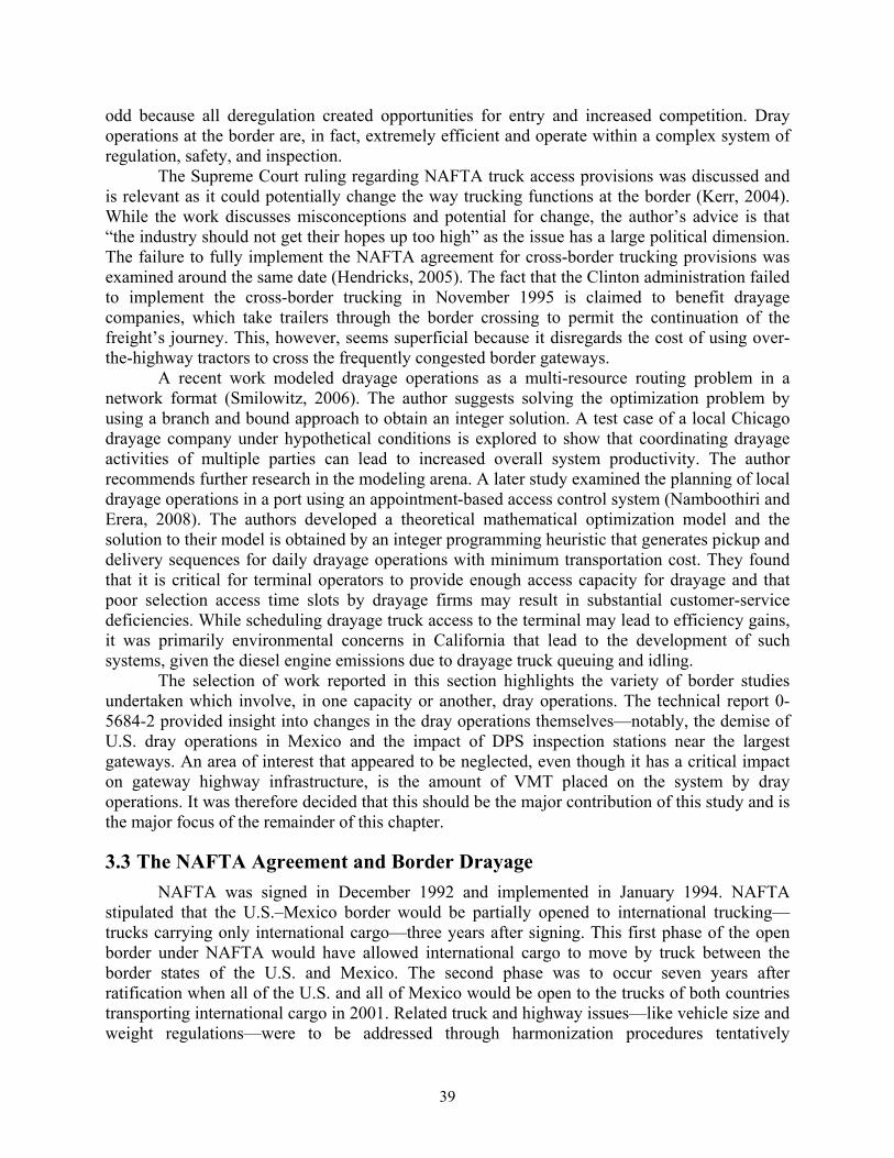
39

odd because all deregulation created opportunities for entry and increased competition. Dray operations at the border are, in fact, extremely efficient and operate within a complex system of regulation, safety, and inspection.

The Supreme Court ruling regarding NAFTA truck access provisions was discussed and is relevant as it could potentially change the way trucking functions at the border (Kerr, 2004). While the work discusses misconceptions and potential for change, the author’s advice is that “the industry should not get their hopes up too high” as the issue has a large political dimension. The failure to fully implement the NAFTA agreement for cross-border trucking provisions was examined around the same date (Hendricks, 2005). The fact that the Clinton administration failed to implement the cross-border trucking in November 1995 is claimed to benefit drayage companies, which take trailers through the border crossing to permit the continuation of the freight’s journey. This, however, seems superficial because it disregards the cost of using over-the-highway tractors to cross the frequently congested border gateways.

A recent work modeled drayage operations as a multi-resource routing problem in a network format (Smilowitz, 2006). The author suggests solving the optimization problem by using a branch and bound approach to obtain an integer solution. A test case of a local Chicago drayage company under hypothetical conditions is explored to show that coordinating drayage activities of multiple parties can lead to increased overall system productivity. The author recommends further research in the modeling arena. A later study examined the planning of local drayage operations in a port using an appointment-based access control system (Namboothiri and Erera, 2008). The authors developed a theoretical mathematical optimization model and the solution to their model is obtained by an integer programming heuristic that generates pickup and delivery sequences for daily drayage operations with minimum transportation cost. They found that it is critical for terminal operators to provide enough access capacity for drayage and that poor selection access time slots by drayage firms may result in substantial customer-service deficiencies. While scheduling drayage truck access to the terminal may lead to efficiency gains, it was primarily environmental concerns in California that lead to the development of such systems, given the diesel engine emissions due to drayage truck queuing and idling.

The selection of work reported in this section highlights the variety of border studies undertaken which involve, in one capacity or another, dray operations. The technical report 0-5684-2 provided insight into changes in the dray operations themselves—notably, the demise of U.S. dray operations in Mexico and the impact of DPS inspection stations near the largest gateways. An area of interest that appeared to be neglected, even though it has a critical impact on gateway highway infrastructure, is the amount of VMT placed on the system by dray operations. It was therefore decided that this should be the major contribution of this study and is the major focus of the remainder of this chapter.

3.3 The NAFTA Agreement and Border Drayage NAFTA was signed in December 1992 and implemented in January 1994. NAFTA

stipulated that the U.S.–Mexico border would be partially opened to international trucking—trucks carrying only international cargo—three years after signing. This first phase of the open border under NAFTA would have allowed international cargo to move by truck between the border states of the U.S. and Mexico. The second phase was to occur seven years after ratification when all of the U.S. and all of Mexico would be open to the trucks of both countries transporting international cargo in 2001. Related truck and highway issues—like vehicle size and weight regulations—were to be addressed through harmonization procedures tentatively

40

scheduled through the entire period. In December 1995, when the first phase of the open border was to begin, the U.S. unilaterally decided not to open the border. Although it was alleged that Mexican trucks were unsafe, it was never demonstrated that this was, in fact, the case. With the exception of a current (2007/8) pilot scheme that permits a small number of Mexican and U.S. trucks to carry international cargo into the U.S. and Mexico, the open border provisions have not been enacted and therefore had a negligible impact on current drayage VMT in the McAllen/Pharr, Laredo, and El Paso areas. It should be noted that although a foreign truck tractor cannot travel into the interior of the U.S. or Mexico, trailers do move into the interior of both countries. Drayage trucks move the trailers northbound and southbound across the border within the commercial border zones at each port.

The border commercial zones are established as areas in gateway cities where international vehicles and non-residents can travel to conduct business without meeting all of the requirements to enter the interior of the U.S. Each border port has a designated commercial zone that in most cases extends beyond city limits. The most significant exception is the commercial zone in the Lower Rio Grande Valley. In the Lower Rio Grande Valley, which includes McAllen/Pharr, the commercial zone is comprised of the area of Cameron, Hidalgo, Starr, and Willacy counties. The commercial zone in Laredo is 8 miles beyond the city limits and the commercial zone in El Paso is 15 miles beyond the city limits. A similar zone exists in Mexico but it does not have the same limits as the U.S.

Dray trucks take empty and full trailers between industrial areas that contain factories, warehouses, and truck transfer facilities on both sides of the border. Dray trucks transferring loaded trailers bound for the interior of Mexico pick up the trailers at a warehouse or truck transfer facilities in the U.S. and take the trailer to an industrial area in Mexico containing a truck transfer yard. After being dropped at a truck transfer facility, the trailer is then attached to a Mexican line haul tractor that will carry the trailer to its destination in Mexico. Northbound dray trucks will reverse this process picking the trailer up at a maquiladora factory or truck transfer yard in Mexico and bringing the trailer to a warehouse or truck transfer facility in the U.S. It is the “three step” process that a majority of researchers have concentrated on and decided that it creates inefficiencies which would be reduced by an open border policy.

3.4 Bridge Crossing Truck Trips The number of commercial bridges in the border cities is critical in the movement of

drayage trucks across the border. There is one commercial bridge in McAllen/Pharr and two each in Laredo and El Paso that are considered in this study. The first step in developing an estimate of drayage truck VMT was to obtain data and establish the number of truck crossing trips over each of the commercial bridges in McAllen/Pharr, Laredo, and El Paso.

It was first necessary to identify data giving the number of trucks crossing the border bridges to estimate the drayage VMT at McAllen/Pharr, Laredo, and El Paso. Two data sources were considered for this task: the TransBorder Freight Data and Truck Crossing data. These data were examined for possible use in developing an estimate of the VMT for drayage trucks in McAllen/Pharr, Laredo, and El Paso. The TransBorder Freight Data is developed by the Bureau of Transportation Statistics (BTS) from trade data provided to the BTS through an agreement with U.S. Customs and Border Protection. This data is available from the Bureau of Transportation Statistics, a sub-unit of the Federal Highway Administration. The truck crossing data consists of bridge counts of the trucks that cross southbound into Mexico and the counts from U.S. Customs for northbound trucks traveling into the U.S. This data is available from the

41

Texas Center for Border Economic and Enterprise Development at Texas A&M International University (TAMIU) in Laredo, Texas.

The TransBorder Freight data was examined by first obtaining data from the BTS web site and was then reviewed monthly for 2007 for possible use in determining the VMT of drayage vehicles at McAllen/Pharr, Laredo, and El Paso. It is important to remember that this data is derived from the export and import trade data collected by U.S. Customs and Border Protection at each port. While the data provides information about the exports and imports of commodities, their value, and partial data about weight, there is no practical way to derive the number of trucks crossing northbound and southbound in the three border cities. Additionally, the TransBorder Freight Data does not have data for individual bridges. Another difficulty with the data is that it shows only the exports and imports of products between the U.S. and Mexico and thus omits exports and imports that cross the border having passed through Mexico—goods from Asia, for example. For these reasons it was determined that using the TransBorder Freight Data would not provide a reasonable estimate of VMT.

The second set of data reports the number of trucks that cross the border in each city. This data was reviewed for 2007 for possible use in determining the VMT of drayage vehicles at McAllen/Pharr, Laredo, and El Paso. TAMIU collects this data, which is derived from the counts of trucks crossing toll bridges southbound into Mexico and counts of trucks that enter U.S. Customs and Border Protection facilities northbound. The original data for southbound crossings is reported to TAMIU by the toll bridge authorities in each border city. The different toll bridge authorities do not all use a common format, making it necessary to use the total truck crossings found in the data. The northbound number of trucks is obtained from U.S. Customs and Border Protection, which counts trucks that enter the U.S. These northbound truck counts are considered to be the most reliable counts. The need for uniformity in developing a data set required that some assumptions and estimates were adopted.

The first important assumption necessary to develop an estimate of the drayage VMT in the three cities was to consider total truck crossings. As mentioned, this was necessary because it was not possible to accurately distinguish in the data between trucks with and without trailers. A second important assumption was that a northbound trip distance was equal to a southbound trip distance within the U.S. Additionally, if data was not available for individual bridges in Laredo or El Paso an estimate of trucks crossing could be derived using a percentage of the total truck traffic based upon data available from the city bridge authorities. The last assumption was that if information about the southbound movement of trucks over a bridge was missing or unavailable, the total number of northbound and southbound trucks would be considered to be equal. Table 3.1 shows the total bridge trips northbound and southbound used in this chapter.

The TAMIU data shows the total northbound and southbound number of trucks at the border cities but does not show northbound and southbound numbers of trucks over each bridge within a city. Therefore, each city except McAllen/Pharr, which has only one bridge, required an estimate of the number of trucks crossing each bridge. In Laredo there are two bridges: the World Trade Bridge and the Columbia Solidarity Bridge. Therefore, it was necessary to develop an estimate of the portion of total northbound and southbound truck crossings that should be allocated to each bridge. An estimate was developed of truck crossings over the two bridges based upon the southbound commercial truck crossings breakdown available from the Laredo Bridge Authority. The Laredo Bridge Authority shows that 77 percent of the southbound trucks use the World Trade Bridge and 23 percent use Columbia Solidarity Bridge. Therefore, the best

42

estimate of crossings over the two bridges is 2,372,974 for the World Trade Bridge and 708,811 for the Columbia Bridge, as shown in Table 3.1.

Table 3.1: McAllen/Pharr, Laredo, and El Paso Total Bridge Crossing Trips

Bridge Northbound Southbound Total

McAllen/Pharr Pharr 485,051 447,165 932,216 Laredo World Trade 1,130,397 1,242,577 2,372,974 Columbia 337,651 371,160 708,811 Laredo Total 1,468,048 1,613,737 3,081,785 El Paso BOTA* 445,950 446,558 892,508 Zaragoza 336,419 335,810 672,229 El Paso Total 782,369 782,368 1,564,737

Source: Data TAMIU and Bridge Authorities *Estimated as explained in Section 3.4

El Paso, like Laredo, has two commercial bridges: Bridge of the Americas (BOTA) and the Ysleta-Zaragoza Bridge. An additional complication in El Paso is the fact that BOTA is a free bridge as established by international treaty and because the bridge is without tolls there are no southbound truck counts (derived from fees) publicly available. In El Paso it was necessary to begin with the total northbound number of trucks as reported by U.S. Customs and Border Protection and to assume that the same numbers of trucks, 782,368, were traveling northbound and southbound. The southbound number of trucks was reported for the Zaragoza Bridge, which is a toll bridge. The southbound truck count was taken to be the total number of trucks, 782,368, minus the reported number of the Zaragoza Bridge, 335,810. It was then estimated that 782,369 – 335,810 = 446,559 would be the southbound crossings at BOTA. Next, the percentage of southbound trucks crossing each bridge was determined. At BOTA the percentage is 446,559/782,369 = 57 percent. This number was then used to allocate the northbound trucks and gives 57 percent to BOTA and 43 percent to Zaragoza. The total estimated number of trucks over each bridge is shown in Table 3.1. Although these estimates are not as precise as other locations, it is believed that they are sufficient to estimate the drayage truck VMT in El Paso.

3.5 Method to Determine Industrial Areas and Vehicle Miles Traveled A six-step process was used in each border city to determine VMT. First, the number of

truck trips across the commercial bridges was determined using the truck crossing data available from TAMIU, as explained earlier and shown in Table 3.1. Second, it was determined by the research team that locations that had industrial areas with significant numbers of warehouse and truck transfer facilities would be appropriate industrial locations to be considered as origins and destinations of dray truck travel in the border cities. These industrial areas were identified by personal knowledge of the researchers, map study, and where possible, interviews. Third, the area of the industrial area in acres was determined using a digital map program. Fourth, the distance of dray truck travel from the international bridge to each of the industrial areas in each city was determined using a digital map program. Fifth, using the area in acres of each industrial area as a percent of the total industrial area in acres in the city, the total number of trips across

43

each bridge was allocated to each industrial area. Sixth, the drayage truck VMT for each city was calculated by multiplying the number of trips to each industrial area in that city by the distance of each trip. As mentioned, a southbound trip and a northbound trip were considered to travel an equal distance. Data could not be used to distinguish between trucks with empty or full trailers or trucks without trailers. Therefore, the total trips by dray trucks was taken to be the number of northbound plus southbound truck trips over each bridge as shown in Table 3.1.

The commercial bridge that serves McAllen is generally referred to as the Pharr Bridge and because all drayage trucks in McAllen use the Pharr Bridge, the term McAllen/Pharr refers to the U.S. drayage area in the vicinity of McAllen and Pharr, Texas. Drayage operations in McAllen/Pharr occur in the deepest border commercial zone on the U.S.–Mexico border. The zone includes Cameron, Hidalgo, Starr, and Willacy counties. The primary movement of dray trucks in McAllen/Pharr is to and from maquiladora factories in Reynosa, Tamaulipas, Mexico. Dray trucks carrying trailers to maquiladora factories pick up the trailer at a warehouse or truck transfer yard within an industrial area in McAllen/Pharr, Texas and deliver the trailer to a maquiladora factory within an industrial area in Reynosa. When the maquiladora factory has produced a full trailer of finished products a dray truck will pick up the trailer and take it to a warehouse or truck transfer facility in McAllen/Pharr. The McAllen/Pharr commercial bridge to Mexico is shown in Figure 3.1. The bridge is located relatively close to the maquiladora factories in Mexico and the industrial areas in the vicinity of Pharr and McAllen, Texas. The data from TAMIU shows that there were 932,216 trips across the Pharr Bridge in 2007. Of these trips, 485,051 were northbound and 447,165 southbound.

Figure 3.1: McAllen/Pharr Commercial Bridge and Industrial Areas

44

There are approximately 947 acres within 9 industrial areas in McAllen/Pharr that are potential origins and destinations for dray truck movements. Figure 3.1 shows the locations and designations of these industrial areas and Table 3.2 shows the industrial designation, location, size in acres, percent of dray trips, distance from the Pharr Bridge to the industrial area, and VMT.

The most dominant of the nine areas is MA3, which is located at West Military and Ware Rd. This industrial area contains 288 acres and is 10.3 miles from the bridge. The area accounts for an estimated 283,504 drayage trips or 30 percent of the dray truck movements. Industrial Area MA3 accounts for 2.9 million miles of the dray VMT in McAllen/Pharr. The next two prominent industrial locations are MA5 and MA6. MA5 is located at East Produce and 10th Street, contains 139 acres, and is 5.7 miles from the bridge. MA6 is located at U.S. 83 and West Polk, contains 124 acres, and is 10.9 miles from the bridge. Although MA5 is slightly larger than MA6, MA6 generates significantly more VMT because it is nearly twice the distance from the bridge.

Three additional large industrial areas in McAllen/Pharr are MA8 at South Cage and East Anoya, MA2 at West Military and South International, and MA4 at South 23rd and West Dicker. MA8 contains 98 acres, is 2.7 miles from the bridge, and accounts for only 0.26 million dray miles. MA2 contains 96 acres, is 11.6 miles from the bridge, and accounts for 1 million miles of the VMT. MA4 contains 82 acres, is 8 miles from the bridge, and accounts for 0.6 million VMT. The remaining industrial areas account for only 120 of the industrial acres in McAllen/Pharr.

Table 3.2: McAllen/Pharr Industrial Areas, Trip Distances, and VMT

Industrial Area Location Acres

% of Trips

Total Trips to Area

Distance Pharr Bridge to Industrial Areas (Miles)

VMT McAllen/Pharr

MA1 Trinity and Business Park Dr 53 0.06 52,173 18.7 975,825

MA2 West Military and South Int'l 96 0.10 94,501 11.6 1,092,229

MA3 West Military and Ware Rd 288 0.30 283,504 10.3 2,924,355

MA4 S 23d and West Dicker Dr 82 0.09 80,720 8.0 647,043

MA5 East Produce and S 10th St 139 0.15 136,830 5.7 782,226

MA6 US 83 and West Polk 124 0.13 122,064 10.9 1,327,362

MA7 East Military and South Road 42 0.04 41,344 2.7 113,040

MA8 S Cage and East Anoya 98 0.10 96,470 2.7 263,760

MA9 US 83 and South Stewart 25 0.03 24,610 11.9 292,081

Total 947 1 932,216 8,417,920

Total NB and SB Trips 932,216 McAllen/Pharr is the dominant land port in the Lower Rio Grande Valley with a total of

932,216 crossings and an estimated 8.4 million dray miles in 2007. Drayage movements in McAllen/Pharr are concentrated between the bridge and MA2, MA3, MA4, MA5, MA7, and MA8. These moves are concentrated along US 281, South 23rd Street, and West Military

Highwaymillion d

L

Lcrossingscrossing percent cBridge isgrade senorthwesDrayage Tables 3.areas, theLaredo W

y. Taken togdray miles at

aredo Indus

Laredo is the s: the Worldnorthbound

cross the Ws located releparated linkst of the Woroperations i

.3 and 3.4 she percentage

World Trade

gether theset McAllen/Ph

strial Areas,

dominant lad Trade Bridd and 1,613,7World Trade latively closk to IH-35. rld Trade Brin Laredo suhow each of e of the totalBridge and

Fig

e industrial harr.

Dray Distan

and port on tdge and the 737 trucks cBridge and

e to industriThe Colum

ridge and noupport the mf the industril acres for ethe Laredo C

gure 3.2: Lar

45

locations ac

nce and Veh

the U.S.–MeColumbia B

crossing soud 23 percential areas as mbia Bridgeot near most movement ofal locations,ach industriColumbia Br

redo Comme

ccount for

icle Miles Tr

exico borderBridge. Of t

uthbound in t cross at Cshown in Fie, however, major indusf deep trade, the acres ofal area, and ridge.

ercial Bridge

5.8 million

Traveled

r with two cothe total of 2007, it is e

Columbia. Tigure 3.2, an

is approximtrial origins

e into the intf each area, the number

es

of the tota

ommercial b1,468,048 trestimated th

The World Tnd is served mately 18 mand destinat

terior of Metotal acres f

r of trips ove

al 8.4

bridge rucks

hat 77 Trade

by a miles tions. exico. for all er the

46

Figure 3.3: Laredo Industrial Areas

There are approximately 3,548 acres within 13 industrial areas in Laredo that are potential origins and destinations for dray truck moves. Figure 3.3 shows the locations and designations of these industrial areas and Tables 3.3 and 3.4 shows the industrial designation. The location, size in acres, percent of dray trips, and distance from the World Trade Bridge is shown in Table 3.3 and the same information for the Columbia Bridge is shown in Table 3.4.

The most dominant of the 13 areas is LD6, located at the intersection of North Mines Road and the Bob Bullock Loop. This industrial area contains 956 acres and is 4 miles from the World Trade Bridge and 18 miles from the Columbia Bridge. The industrial area contains several warehouses and truck transfer facilities. LD6 accounts for an estimated 658,687 drayage trips over the World Trade Bridge and 196,751 trips over the Columbia Bridge. Total annual VMT to this industrial area over the World Trade Bridge is 2.7 million miles and over the Columbia Bridge is 3.6 million miles.

47

Near to LD6 are industrial areas LD4 and LD5, which are located along West Mines Road, 2.3 miles and 2 miles northwest of IH 35 respectively. LD4 has 438 acres and is 4 miles from the World Trade Bridge and 16 miles from the Columbia Bridge. LD5 has 224 acres and is 3 miles from the World Trade Bridge and 17 miles from the Columbia Bridge. The areas account for 1.3 million and 0.4 million miles of VMT over the World Trade Bridge and 1.5 million and 0.8 million miles of VMT over the Columbia Bridge. Taken together, LD6, LD4, and LD5 account for 4.4 million miles of drayage VMT over the World Trade Bridge and 5.8 million miles of the VMT over the Columbia Bridge.

The second largest industrial area in Laredo is LD1 at the intersection of IH 35 and Uniroyal Drive. This industrial area contains 675 acres and is 10 miles from the World Trade Bridge and 26 miles from the Columbia Bridge. There are 465,077 estimated trips to this industrial area over the World Trade Bridge and 138,919 over the Columbia Bridge. This area accounts for more VMT than any other area in Laredo with 4.6 million miles over the World Trade Bridge and 3.7 million miles over the Columbia Bridge.

Two additional large industrial areas are LD3 and LD7. LD3, located northeast of the intersection of IH 35 and Bob Bullock Loop, has 375 acres and is 4 miles from the World Trade Bridge and 21 miles from the Columbia Bridge. This area accounts for 258,376 trips and 1.1 million miles of VMT over the World Trade Bridge and 77,177 trips and 1.6 million dray VMT over Columbia. LD7 is located north of the intersection of IH 35 and Mines Road. It has 283 acres and is 3 miles from the World Trade Bridge and 20 miles from the Columbia Bridge. This industrial area accounts for 194,988 trips and 0.6 million dray miles over the World Trade Bridge and 58,243 trips and 1.2 million dray VMT over the Columbia Bridge at Laredo.

48

Table 3.3: Laredo World Trade Bridge (WTB), Industrial Areas, Trip Distances, and VMT

Industrial Area Location

Area (Acres)

% of Trips to Area

WTB Total Trips to and From Area

Distance (Miles) WTB to Industrial Area

WTB VMT to Industrial Areas

LD1 LIA IH 35 and Uniroyal Dr. 675 0.19 465,077 10 4,623,896

LD2 IH 35 and U. Pacific Rail 45 0.01 31,005 10 304,406

LD3 Bob Bullock and IH 35 NE 375 0.11 258,376 4 1,107,808

LD4 West Mines Road 2.3 Mi N of IH-34 438 0.12 301,783 4 1,256,415

LD5 West Mines Road 2 Mi N of IH 35 224 0.06 154,337 3 393,202

LD6 N Mines Rd. and BB Loop 956 0.27 658,687 4 2,701,383

LD7 N Mines Road and IH 35 283 0.08 194,988 3 593,700

LD8 Mines Road-Del Mar 86 0.02 59,254 3 176,736

LD9 IH 35 and Industrial Blvd 83 0.02 57,187 5 266,516

LD10 Santa Maria and West Carlton 185 0.05 127,466 6 736,612

LD11 Santa Rita and Franklin St 90 0.03 62,010 8 481,656

LD12 Bob Bullock and US 59 16 0.00 11,024 11 116,454

LD13 Bob Bullock and KCS Rail 92 0.03 63,388 11 720,814

Total 3548 13,479,598

49

Table 3.4: Laredo Columbia Bridge, Industrial Areas, Trip Distances, and VMT

Industrial Area Location

Area (Acres)

% of Trips to Area

Columbia Bridge Trips to and from Area

Miles Distance Columbia to Industrial Area

Columbia VMT to Industrial Areas

LD1 LIA IH 35 and Uniroyal Dr. 675 0.19 138,919 26 3,668,716

LD2 IH 35 and U. Pacific Rail 45 0.01 9,261 26 243,430

LD3 Bob Bullock and IH 35 NE 375 0.11 77,177 21 1,601,766

LD4 West Mines Road 2.3 Mi N of IH 34 438 0.12 90,143 16 1,461,962

LD5 West Mines Road 2 Mi N of IH 35 224 0.06 46,101 17 784,910

LD6 N Mines Rd. and BB Loop 956 0.27 196,751 18 3,582,176

LD7 N Mines Road and IH 35 283 0.08 58,243 20 1,150,893

LD8 Mines Road-Del Mar 86 0.02 17,699 20 355,240

LD9 IH 35 and Industrial Blvd 83 0.02 17,082 21 365,139

LD10 Santa Maria and West Carlton 185 0.05 38,074 22 856,449

LD11 Santa Rita and Franklin St 90 0.03 18,523 24 451,180

LD12 Bob Bullock and US 59 16 0.00 3,293 27 89,418

LD13 Bob Bullock and KCS Rail 92 0.03 18,934 28 529,446

Total 3548 730,200 15,140,726 The estimated total area in acres and distance traveled to each industrial area using the

World Trade Bridge and the Columbia Bridge is shown in Tables 3.3 and 3.4. In all cases the distance traveled to Laredo industrial areas utilizing the Columbia Bridge is significantly more, often more than twice, the distance a dray truck travels using the World Trade Bridge. The total VMT over the World Trade Bridge is 13.5 million miles while the Columbia Bridge has a total of 15.1 million VMT. The total annual VMT of drayage trucks in Laredo is estimated to be 28.6 million miles. Drayage movements in Laredo are concentrated along the Mines Road, north of Laredo along IH 35, and along Bob Bullock Loop.

El Paso Industrial Areas, Dray Distance and Vehicle Miles Traveled

El Paso is the second largest port on the Texas–Mexico border. Drayage movements at El Paso are primarily to or from maquiladora factories in Mexico. There are two commercial bridges in El Paso: the Bridge of the Americas and the Zaragoza Bridge. Of the total of 1,564,737 trucks crossing the border in El Paso, it is estimated that 892,508 or 57 percent of these trips cross the Bridge of the Americas and 672,229 or 43 percent cross Zaragoza. These bridge locations are shown in Figure 3.4. The Bridge of the Americas is located relatively close to the older industrial areas. The Zaragoza Bridge is located near the new industrial areas. An estimated total of 1,564,737 dray trucks crossed the border at El Paso in 2007.

The search for industrial locations in El Paso was conducted using map study, interviews, and observation. Twelve dominant origin/destination industrial areas were identified. Each of

50

these origin/destinations had significant factory, distribution, and truck transfer facilities. These origin/destinations are shown in Figure 3.4.

Figure 3.4: El Paso Commercial Bridges and Industrial Areas

A large cluster of these industrial locations is comprised of EP7, EP8, EP9, and EP10. These industrial areas are located between the Zaragoza Bridge and IH 10. EP9 is the largest of these areas and is located at the intersection of IH 10 and North Zaragoza and has 612 acres. It is 12 miles from BOTA and 5 miles from Zaragoza. EP9 accounts for 192,737 trips and 2.3 million dray miles over BOTA and 145,167 trips and .7 million miles of VMT over Zaragoza. Within this cluster, the next largest industrial area is EP10, located at IH 10 and Joe Battle. It has 316 acres and is 14 miles from BOTA and 5 miles from Zaragoza. This industrial location accounts for 99,518 trips and1.4 million dray miles over BOTA and 74,956 trips and 0.4 million VMT over Zaragoza. Next in size is EP8 with 216 acres and EP7 with 148 acres. EP8 is located south of the intersection of Pan American Highway and Highway 375, 11 miles from BOTA and 1 mile from Zaragoza and accounts for 68,025 trips over BOTA and 51,235 trips over Zaragoza and 0.8 million of dray miles over BOTA and 0.07 million miles of VMT over Zaragoza. EP7 is located north of the intersection of the Pan American Highway and Highway 375. It is 12 miles from BOTA and 1 mile from Zaragoza and accounts for 46,610 trips and 0.5 million VMT crossing at BOTA and 35,106 trips and 0.04 million of VMT crossing at Zaragoza.

EP3, the second largest industrial area in El Paso, is located adjacent to the El Paso International Airport. It has 554 acres and is 5 miles from BOTA and 15 miles from Zaragoza. EP3 accounts for 174,471 trips and 0.9 million VMT crossing at BOTA and 131,410 and 2 million miles of VMT crossing at Zaragoza.

The most westerly industrial location is EP1, located at the intersection of IH 10 and Paseo Del Norte. It is comprised of 360 acres and is 19 miles from BOTA and 30 miles from Zaragoza. It accounts for 113,374 trips and 2.1 million dray miles over BOTA and 85,392 trips and 2.5 million dray miles over Zaragoza. In the opposite direction is EP12 at Horizon and

51

Darrington Road. This area has 218 acres and is 21 miles from BOTA and 12 miles from Zaragoza and this industrial area accounts for 68,655 trips and 1.4 million miles crossing at BOTA and 51,710 trips and 0.6 million dray miles crossing at Zaragoza.

Tables 3.5 and 3.6 present the data for both El Paso bridges.

Table 3.5: El Paso BOTA Bridge, Industrial Areas, Trip Distances, and VMT


% of Trips=Total Area/Industrial Area

BOTA Number of Trips

Distance BOTA to Industrial Area

Total VMT Over BOTA

EP1 IH 10 PaseoDelNorte 360 0.13 113,374 19 2,155,756

EP2 Intermodal Canal Rd 46 0.02 14,487 3 45,910

EP3 Airport–Leigh Fisher 554 0.20 174,471 5 932,361

EP4 IH 10 Hawkins 63 0.02 19,841 6 109,725

EP5 Intermodal Stiles Dr 87 0.03 27,399 5 127,690

EP6 IH 10–N Lee Trevino 125 0.04 39,366 10 379,156

EP7 N LP 375–Pan American 148 0.05 46,610 12 538,704

EP8 S LP 375–Pan American 216 0.08 68,025 11 773,536

EP9 IH 10–N Zaragoza 612 0.22 192,737 12 2,275,521

EP10 IH 10–LP 375 316 0.11 99,518 14 1,385,195

EP11 IH 10–Horizon 89 0.03 28,029 17 473,734

EP12 Horizon Rd–Darrington Rd 218 0.08 68,655 21 1,441,946 2,834 892,509 10,639,233Total BOTA Trips 892,509

52

Table 3.6: El Paso Zaragoza Bridge, Industrial Areas, Trip Distances, and VMT


% of Trips=Total Area/Industrial Area

Zaragoza Number of Trips

Miles Distance Zaragoza to Industrial Areas

Total VMT Over Zaragoza

EP1 IH 10 PaseoDelNorte 360 0.13 85,392 30 2,546,970EP2 Intermodal Canal Rd 46 0.02 10,911 13 143,061EP3 Airport–Leigh Fisher 554 0.20 131,410 15 1,992,415EP4 IH 10 Hawkins 63 0.02 14,944 9 130,002EP5 Intermodal Stiles Dr 87 0.03 20,637 8 156,444EP6 IH 10–N Lee Trevino 125 0.04 29,650 6 171,346EP7 N LP 375–Pan American 148 0.05 35,106 1 43,629EP8 S LP 375–Pan American 216 0.08 51,235 1 66,858EP9 IH 10–N Zaragoza 612 0.22 145,167 5 685,560EP10 IH 10–LP 375 316 0.11 74,956 5 363,297EP11 IH 10–Horizon 89 0.03 21,111 8 167,911

EP12 Horizon Rd–Darrington Rd 218 0.08 51,710 12 623,359

2,834 672,229 7,090,851Total Zaragoza Trips 672,229

Drayage movements in El Paso are concentrated along highway 375 near the Zaragoza

Bridge and along IH 10 especially in the vicinity of the intersections of IH 10 and North Zaragoza and IH 10 and Joe Battle. There are also large concentrations of drayage trucks at the international airport. The major concentration west along IH 10 is at IH 10 and Paseo Del Norte. The most eastern concentration is at Horizon and Darrington Road. El Paso has 10.6 million dray truck miles that travel over BOTA and 7.1 million miles over Zaragoza.

3.6 Concluding Remarks This section provided, within the limits of the project resources, an estimate of the major

origin and destination industrial areas and annual VMT of drayage trucks in 2007 within the commercial zones of the border cities of McAllen/Pharr, Laredo, and El Paso. It was determined that there was a total of 8.4 million VMT of dray trucks in McAllen, 28.6 million VMT at Laredo, and 17.7 million at El Paso. High concentrations of drayage truck travel in McAllen are along US 281, South 23d Street, and West Military Highway. Drayage movements in Laredo are concentrated along the Mines Road, north of Laredo along IH 35, and along Bob Bullock Loop. In El Paso drayage movements are concentrated along highway 375 near the Zaragoza Bridge, in the vicinity of the international airport, and along IH 10 especially near the intersections of IH 10 and North Zaragoza and IH 10 and Joe Battle.

Dray operations at the border are more extensive than those that cross the international bridges across the Rio Grande, though these routes represent the dominant type of dray border operations. This method does not capture much of the U.S. dray operations which comprise (a) intra-warehouse moves within the commercial zones, (b) gateway to gateway moves (for

53

example, Pharr to Laredo), (c) gateway to San Antonio and Houston customers, and finally (d) intermodal moves from the rail terminals at El Paso and Laredo. Gateway to major city moves like San Antonio is a growing segment for U.S. dray companies who are, in many cases, using the post-2005 tractors to meet reliability standards. The use of dray services at rail intermodal border terminals is the subject of the next chapter and complements the findings of the bridge estimates reported in this chapter.

55

Chapter 4. Laredo Rail Intermodal Terminal Dray Survey

4.1 Background Chapter 3 provided a description of NAFTA and estimated the ways in which the cross-

border dray VMT at the leading gateways have been impacted by its implementation. Since the passage of the agreement, Laredo has strengthened its position as the principal hub for NAFTA truck traffic. However, rail shipments through Laredo are also growing both in tonnage and in value. The Laredo gateway connects Mexico City and the industrial centers of San Luis Potosi and Monterrey with Houston, Dallas, Kansas City, and Chicago. The Union Pacific and the former Tex-Mex railroads (now KCS de Mexico) were first to provide U.S.–Mexico rail service through Laredo and Union Pacific; they were operating a regular double stack service from Chicago to Mexico City in the early 1990s. The rail connection linking these industrial centers is made more viable by the increased containerized cargo and bulk/auto traffic being generated by NAFTA industries. Intermodal rail, to successfully compete with trucking, must create a critical level of demand over routes where rail efficiencies are present. In 1993, Union Pacific broke ground on an intermodal terminal called Port Laredo, some 12 miles from the cross border rail bridge downtown. It was so successful that it was enlarged around 6 years later to its current size and shape. The rail yard located at Laredo allows Union Pacific to generate this critical mass of containerized cargo. In order to better describe dray activity connected with rail activity in Laredo, a case study of Port Laredo was performed. The principal element of the case study was a survey conducted August 11 and 12, 2008, at the Port gates along with interviews of UP officials and local dray carriers. The following section outlines the role that drayage plays at this new intermodal facility.

4.2 Survey Design The goal of the survey was to describe the types of trucks, drivers, firms, and cargo

handled at Port Laredo and to provide insight into the origins and destinations of the cargo. The survey document is given in Appendix B. The basic structure of the survey was designed to closely correspond to the previous survey performed at the Houston Englewood terminal; however, certain questions were altered in order to better reflect local conditions.

Surveys were conducted at the Union Pacific facility at Laredo with the active participation of the Union Pacific officials as well as that of Railtrax, the third-party logistics operator (3PL) that is employed to handle operations at the facility. The principal point of contact was Mr. Robert de Alba, Manager of Intermodal Operations at Port Laredo.

The survey was designed to capture many of the same elements that were previously captured at the Englewood rail yard in Houston, Texas and described in Chapter 2. Surveys were segregated for incoming and outgoing loads. The surveys contained questions regarding the working environment for the truck and the driver, the model and age of the truck, the origins and destinations of the cargo, the type of cargo, the frequency with which drivers make deliveries to the rail terminal, the driver’s level of satisfaction with the performance of the terminal, and any recommendations the drivers might have for improvement of the terminal operations. Surveys were conducted at the entry and exit point for dray trucks to the rail yard gate by trained interviewers and were conducted principally in Spanish. Drivers answered the questions while waiting for their paperwork to be completed—a process that usually only took about five

56

minutes. Therefore, the surveyors had to secure the answer to almost 20 questions within this short time frame. Key results from the survey included a description of the structure of the industry such as the principle firms currently serving the rail facility, the patterns of ownership, and origin and destination data.

The Union Pacific rail yard located at Laredo is unlike the Englewood yard in Houston, which was previously used for chemicals when controlled by Southern Pacific and only later retrofitted for containers. In contrast, Port Laredo was designed specifically for its current purpose. Discussions for intermodal services between Laredo and Mexico City were started in 1991 when Chrysler sought a double-stack intermodal service to ship auto parts to factories in and near Mexico City.6 Port Laredo grew rapidly after the privatization of the Mexican National Railway, which allowed the rapid improvement of the line leading from Laredo to Mexico City. There were significant growing pains for the Port in the late 1990s and Union Pacific was still struggling to incorporate its acquisition of the Southern Pacific while simultaneously establishing a relationship with the newly privatized TFM (Transportación Ferroviaria Mexicana), which had been created under privatization and purchased by the Kansas City Southern and the Transportacion Maritima Mexicana (TMM). Although TFM was rapidly improving, it still suffered from the legacy of underinvestment from the Mexican National Railways. In 1998 Union Pacific suffered a severe logjam on the Laredo gateway tied to the lack of capacity on the bridge linking Laredo to Nuevo Laredo. This caused trains to be backed up through several states and forced the railway to “embargo” traffic bound for Mexico for a period of two weeks to allow the congestion to clear.7 After overcoming these growing pains, Port Laredo has now established a key niche despite the fact that its largest customers—the auto manufacturers—have been in a state of decline as auto plants scaled back production in late 2008.

4.3 Cargo Profile The survey results showed that approximately half of the drivers knew, at least in broad

terms, what type of cargo they were carrying. Also, the drivers were much more likely to be able to identify the cargo type of inbound loads as opposed to outbound (Tables 4.1 and 4.2). For outbound loads, of the 50 drivers who participated in the outbound portion of the survey, 23 drivers would not/could not identify the type of cargo they were taking out of the facility. For inbound loads, 10 drivers answered “Empty” when queried as to the cargo type while only one surveyed driver gave this answer for an outbound load. As can be seen from the outbound data, the percentage of drivers without information on the cargo type means that it is difficult to draw conclusions as to the major commodities handled for outbound shipments.

6 “Special Report on Mexico: Railways forge new links with US system,” Lloyd's List, January 25, 1991, Pg. 8, 394 words 7 “Union Pacific to Ease Its Mexican Embargo,” The New York Times, April 10, 1998

57

Table 4.1: Cargo Type responses for Inbound Shipments: 59 Total responses Automotive Parts 8 Appliances 11 Medical Products 3 Aluminum 4 Food (Fruit Juice) 1 Building Supplies (Tile, Paint, Lumber) 4 N/A or Doesn’t know 3

Table 4.2: Cargo Type Responses for outbound Shipments Automotive Parts 6 Furniture 2 Appliances 3 N/A or Doesn’t know 23

The survey results show that containers and trailers were almost evenly split with 55

containers and 52 trailers. There does not appear to be a strong segregation in terms of which cargoes move by trailer versus which move by container. Most of the trains that are loaded or unloaded by cranes at Port Laredo are purely intermodal but a percentage are mixed trains that contain both containerized and non-containerized cargo. Port Laredo also has a switching yard to make up trains of various configurations. All of the rail containers on the yard were grounded on chassis. There is currently no stacked area and the terminal has no plans to move to stacked operations in the foreseeable future. When compared with other intermodal rail facilities in Texas, the rail facility at Port Laredo experiences relatively little congestion at the gates. When drivers do encounter a bottleneck it is more frequently prior to the entrance to the terminal due to the fact that the road leading to the facility crosses the main Union Pacific track. Therefore, drivers have to wait if a train is passing. Deliveries to the rail yard are often the second stage of the delivery process. Oftentimes a different dray driver will move a box across the border to a yard immediately on the other side of the border, as described in Chapter 3. Then, a second driver will make the delivery from this yard to the rail terminal. This separation of labor occurs if there are delays crossing between Nuevo Laredo and Laredo, or (more frequently) it represents a transfer of ownership within the broker system. The terminal handles both trailer on flat car and double-stack 40- and 53-foot containers. The double-stack 53-foot containers are almost exclusively owned by Pacer Global Logistics, which has an office on site. Many trailers on flat cars are owned by Schneider, and the Schneider yard on the Mines Road was the most common point of destination for the trucks in the survey.

The port principally handles domestic boxes that are moving on the north–south corridor to Chicago. In some cases, the dedicated intermodal trains terminate in Laredo and in other cases they move southbound to Mexico City. Port Laredo receives only about ten containers per day coming directly from Asia. These containers, which are 40 feet in length, arrive alongside other types of traffic on a “mixed train.” Still, the profile of containers coming into and out of Laredo is overwhelmingly domestic 53-foot containers. The container storage area runs alongside the

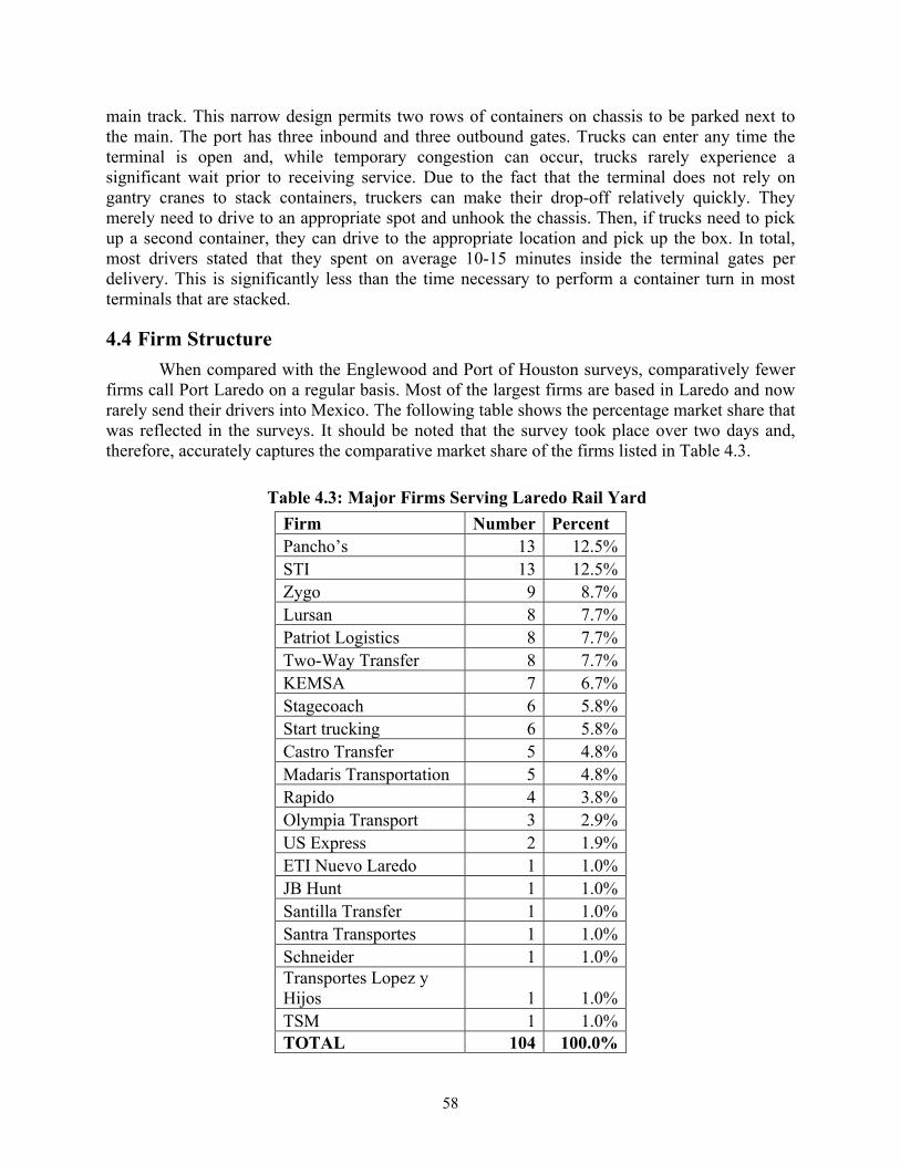
58

main track. This narrow design permits two rows of containers on chassis to be parked next to the main. The port has three inbound and three outbound gates. Trucks can enter any time the terminal is open and, while temporary congestion can occur, trucks rarely experience a significant wait prior to receiving service. Due to the fact that the terminal does not rely on gantry cranes to stack containers, truckers can make their drop-off relatively quickly. They merely need to drive to an appropriate spot and unhook the chassis. Then, if trucks need to pick up a second container, they can drive to the appropriate location and pick up the box. In total, most drivers stated that they spent on average 10-15 minutes inside the terminal gates per delivery. This is significantly less than the time necessary to perform a container turn in most terminals that are stacked.

4.4 Firm Structure When compared with the Englewood and Port of Houston surveys, comparatively fewer

firms call Port Laredo on a regular basis. Most of the largest firms are based in Laredo and now rarely send their drivers into Mexico. The following table shows the percentage market share that was reflected in the surveys. It should be noted that the survey took place over two days and, therefore, accurately captures the comparative market share of the firms listed in Table 4.3.

Table 4.3: Major Firms Serving Laredo Rail Yard Firm Number Percent Pancho’s 13 12.5%STI 13 12.5%Zygo 9 8.7%Lursan 8 7.7%Patriot Logistics 8 7.7%Two-Way Transfer 8 7.7%KEMSA 7 6.7%Stagecoach 6 5.8%Start trucking 6 5.8%Castro Transfer 5 4.8%Madaris Transportation 5 4.8%Rapido 4 3.8%Olympia Transport 3 2.9%US Express 2 1.9%ETI Nuevo Laredo 1 1.0%JB Hunt 1 1.0%Santilla Transfer 1 1.0%Santra Transportes 1 1.0%Schneider 1 1.0%Transportes Lopez y Hijos 1 1.0%TSM 1 1.0%TOTAL 104 100.0%

59

The role played by these firms is somewhat different depending on their size and location. Texas firms operate almost exclusively within the territory of the United States and are based in Laredo. These firms pick up loads from yards on the U.S. side and deliver them to Port Laredo. Other firms are headquartered in Nuevo Laredo and send drivers with loads directly across the border to Port Laredo without making this intermediate stop. Firms that perform cross-border drayage include KEMSA and Two-Way Transfer. It is logical to examine Mexican-domiciled firms in a separate category than firms based in the United States. One hypothesis could be that Mexican firms would have older trucks with higher emissions and younger, less experienced drivers. These metrics would either confirm or deny the assumption that cross-border Mexican dray trucks are more or less safe than an American dray trucks operating within the same market and delivery between the two same customers. Unfortunately, given that there are comparatively few trucks that come directly from Mexico carrying containers, the sample size of these trucks in the survey is too small to calculate if the two populations are different. However, examining KEMSA as a representative Mexican-domiciled carrier reveals that its fleet is not significantly different from many American dray firms. In fact, some American firms had older trucks, based on the survey results.

When completing the surveys at Port Laredo, the researchers were told by UP that in the evening hours, the percentage of drivers arriving directly from Mexico to Port Laredo is comparatively higher than during the peak daytime hours. This regular evening surge of Mexican trucks, which occurred too late to be captured in the survey, is tied to production schedules at maquiladora factories in Nuevo Laredo. The incentive for Mexican-domiciled trucks to cross at night is enhanced by the fact that bridge congestion is often lessened, yet sometimes these late night deliveries are because a driver has been delayed by customs. The pattern is pronounced and, by 10:00 or 11:00 p.m., shortly before the rail yard closes, arrivals are almost exclusively from Mexico.8 The disadvantage of making deliveries at night is that these loads, having missed the cutoff time for rail deliveries, will not be loaded onto the railcars and may miss a rail departure.

All but one of the drivers working for KEMSA reported that they worked in Nuevo Laredo and all reported that they are either coming from or going directly to a location in Nuevo Laredo. Other firms whose drivers reported coming from or going to a location in Nuevo Laredo directly included “Transportes Lopez y Hijos,” Two-Way Transfer, and ETI Nuevo Laredo. The average fleet profile age for the trucks coming directly from Mexico is listed in Table 4.4.

8 Interviews with RailTrax shift workers, August 11 and 12, 2008

60

Table 4.4: Mexico Domiciled Trucks Firm Truck make Model year Mileage

KEMSA Freightliner 1998 14870 KEMSA Freightliner 1996 830670 KEMSA N/A 1997 6178832 KEMSA International 1994 KEMSA Freightliner 1996 KEMSA International 1996 900000 KEMSA Freightliner 1987 1155033 Two-Way Transfer Freightliner 2000 83000 Two-Way Transfer Freightliner 1995 761821 Two-Way Transfer Freightliner 2002 1482856 Two-Way Transfer Freightliner 1998 782520 Two-Way Transfer International 1995 800000 Two-Way Transfer Freightliner Two-Way Transfer International 1995 602155 Two-Way Transfer Freightliner 1998 Transportes Lopez y Hijos Kenworth 1992 900000

Although the sample size for this group is small, it appears that the age profile for the

trucks coming to Port Laredo directly from Mexico and whose drivers live within Mexico is similar to that of trucks coming from yards within the United States. The average model year of the trucks from this sample is 1996. This is slightly lower than the average for the total sample. It should be noted that there is one KEMSA truck with model year of 1987. This one measurement significantly lowered the total average for the truck fleet in the sample. If this truck had been registered in Texas it would have been an ideal candidate for a scrapping and replacement program to boost the air quality of the region. However, given that the trucks are owned by a Mexican firm and registered in Mexico, currently there is no program that would allow a grant to be given to KEMSA that would induce the firm to scrap this old vehicle and replace it with a new vehicle. Therefore, this is one example in which the ownership patterns of an international fleet may make the goal of modernizing the fleet comparatively more difficult when compared with the dray fleet operating at a domestic port or purely domestic rail facility.

In summary, there was only one vehicle from the sample that was manufactured the in 1980s. Of all of the other trucks, none were older than 1994. Only a handful were older than 1996. Trucks from model year 1996 made up 20 percent of the total sample—a very high percentage of the total sample (see Figure 4.1). This is not an accident. Pancho Quesada, who heads one of the largest firms in the Laredo market, told the researchers that he specifically seeks out trucks of a particular age and mileage: specifically, trucks that have at least 500,000 miles but not more than 800,000. Trucks from the 2001 model year were also very popular, constituting 15 percent of the total sample.

61

Figure 4.1: Frequency of Truck Model Age

The surveys recorded three trucks that had a 2007 model year. Some 2007 trucks on the market were equipped with 2006 engines manufactured prior to the federal emissions mandate going into effect. It is not clear from the survey results whether or not these trucks in this sample had 2007 EPA-certified engines or whether not they were 2007 cabs with 2006 engines. Given that both of the 2007 trucks belonged to Stagecoach, itself a major player in the Laredo market, the researchers interviewed Stagecoach’s terminal manager who confirmed that the firm had recently purchased a series of 2007 International trucks that were supposed to deliver superior fuel economy and performance with a lower cost and that these trucks had EPA-certified 2007 engines. There was also one 2008 tractor included in the sample. However, the researchers found that it belonged to a firm, US Express, that is a national carrier and whose driver reported that he was a long haul driver, not a dray driver. A follow-up conversation with the Laredo office of US Express confirmed that no trucks involved in purely local drayage would be newer than 2005.9 Owner-operators make up a distinct minority of trucks servicing Port Laredo. One firm that still uses owner operators, Start Trucking, stated that it had four owner-operators and four company trucks and that the firm made approximately 40 trips to Port Laredo per week. There was no distinction, according to the firm, in the type of operations performed by the owner-operators as opposed to the company-owned trucks.10

If more firms follow the Stagecoach model and voluntarily modernize their fleet based solely on their own internal economics, this bodes quite well for the environmental performance of the Port Laredo dray fleet in coming years. Stagecoach is not yet the biggest player in the port Laredo service. The other major firms in the survey, STI and Pancho’s, also had clearly identifiable characteristics for their fleets. Of the eight responses for STI in which the driver knew the age of the truck (no driver is an owner-operator), one truck was a model year 2000, six were 2001, and one was a 2006.

9 Interview with US Express, Sep 8, 2008 10 Interview with Start Trucking, Sep 8, 2008

0

2

4

6

8

10

12

14

16

1993 1994 1995 1996 1997 1998 1999 2000 2001 2002 2003 2004 2005 2006 2007 2008

Truck Age Frequency at Port Laredo

Frequency

62

Of the other firms that have a prominent showing in the survey results, Pancho’s is a locally owned firm that uses the far more traditional model of dray trucks that have on average 800,000 miles. The researchers’ discussions with Mr. Quesada confirm that he targets vehicles that are retired long haul tractors but can be used quite effectively for live local dray service for a period of years until they can no longer be cost effectively maintained. Extensive interviews were performed with both of these firms that revealed far more that could have been learned simply through driver surveys.

4.5 Driver Hours On average, drivers reported to work 9.5 hours per day and 50 hours per week. The

following distributions (Table 4.5) show the percentile rank of drivers who reported to working the following number of hours per day. For example, drivers who state that they work 9 hours a day are in the 50th percentile.

Table 4.5: Percentile ranking for drivers in reported hours worked per day and per week 10th 8 40 20th 8 40 30th 8 45 40th 8.8 50 50th 9 50 60th 10 52.2 70th 10 57 80th 11 60 90th 12 60 95th 12 65

The overwhelming majority of drivers work on the U.S. side of the border in Laredo. Of

108 respondents, 73 reported that they worked in Laredo while 22 reported working in Nuevo Laredo. Two drivers reported working in both San Antonio and Laredo and one reported working in Eagle Pass. Two drivers stated that they worked nationwide and were making long distance deliveries to Port Laredo. For all practical purposes, all of the drivers making deliveries to Port Laredo work out of the Laredo/Nuevo Laredo metropolitan area.

Despite the fact that most drivers currently work in Laredo on the U.S. side of the border, Nuevo Laredo was the most frequently cited place of birth for the drivers. In total, 31 drivers reported that they had been born in Nuevo Laredo while 20 reported that they had been born in Laredo. In addition, 20 drivers reported that they had been born in other cities within Mexico and one reported to have been born in Nicaragua.

63

4.6 Cargo Origins and Destinations As stated, while much of the cargo that is arriving at Port Laredo was generated in

Mexico, a much smaller percentage is being delivered directly from Mexico by the same truck that transferred the cargo across the border. With one exception, all of the respondents reported that their trip originated in Laredo. Within Laredo, the origins were largely concentrated from industrial parks around a narrow strip along 1472 to the west of IH 35. Destinations of cargo were quite similar; however, there were a greater number of deliveries to the east side of IH 35. In short, the origins and destinations for dray movements from Port Laredo are incredibly concentrated around a very small geographic area. Many of the deliveries move between the northwest and northeast side of the city, thereby having little impact on traffic in the downtown area. As is the case with drayage in Houston, the movements of dray vehicles to the Port are limited to a few critical corridors. In the case of dray movements to Port Laredo, Mines Road (1472), particularly to the north of Highway 20, is the principal corridor. Relatively few drivers reported origins in Central Laredo. In the map in Figure 4.2, each unique destination is represented by a marker. Therefore, the presence of one marker may refer to more than one respondent who listed that address as his point of origin. As noted, several drivers reported coming directly from Nuevo Laredo and did not provide specific addresses. Therefore, on the map Nuevo Laredo is represented by a single centroid marker that does not reference a specific location. In addition, one driver reported that his trip/load originated in Eagle Pass. This data point does not appear on the map so as to better show the precise origins for the Laredo area.

Figure 4.2: Map of trip origins (broad view)

Dwas seenLaredo (sindustria

Awith anot

Destinations n. Specificalslightly) to tl park and C

Figure 4.

As can be seether center o

for loads arlly, several the north of t

Carriers Driv

.3: Map of lo

en in Figureof activity im

re very simildrivers repothe rail yarde.

ocations of t

e 4.4, the mammediately t

64

lar to originorted destina

(see Figure

truck origins

ajority of deto the north o

ns yet slightlations in the4.3). These

s to Port Lar

estinations arof the city.

ly more geoe immediatewere delive

redo (narrow

re located al

graphic divee vicinity ofries to the U

w view)

long Mines

ersity f Port

Unitec

Road

Mresults focomparedthe port possible by the quthe port, congestioof the Mthey madColumbiuse has s

Most of the ound that thd to drivers on average by the close

uick turnarouand by the

on and delayMexican drive

de frequent a crossing, wseveral direc

F

drivers whohe users of t

at the Port of 26 times e proximity und time thafact that mo

ys that regulers from firmtrips to Po

which is knoct and indire

Figure 4.4: M

o call Port Lthe facility dof Houston per week (mof the pointat drivers reost drivers arar border croms such as rt Laredo aown to be aect impacts

65

Map of trip d

Laredo do sodid so with or the Englemedian 25). ts of origin, ceive when re not requirossers must KEMSA an

also reporteda less congeson operation

destinations

o several timfar greater

ewood rail yThis high f

as is made cpicking up

red to cross face. It shou

nd Two-Wayd that they sted point ons at Laredo

mes every dfrequency o

yard. Driverfrequency ofclear by the or dropping the border a

uld also be ny Transfer wfrequently uf crossing. To. From disc

day. The reseon average ws reported tof service is mpreceding moff containe

and deal witnoted that sewho reportedused the CaThe frequencussions wit

earch when o call made maps, ers at th the everal d that amino cy of th the

66

staff at Port Laredo, it was clear that the intimate familiarity of the drivers with operations at the port was a helpful factor in ensuring that drivers adhered to all of the policies of the port and operations ran smoothly. Procedures for trucks entering or leaving the terminal, such as the policy of having drivers switch off their engines while waiting for their paperwork to be completed, were followed almost without exception by the drivers. The good working relationship between dray drivers and terminal employees was demonstrated by the responses to questions regarding the level of service of the Port. Ninety percent of drivers reported that they were satisfied with the overall efficiency of operations at the Port. Of those who stated that they were unsatisfied or neutral with regard to the operation of the port, three were drivers from Nuevo Laredo-based firms and the rest were drivers from Laredo.

4.7 Operational Efficiency As mentioned previously, wait time for trucks entering the terminal and trucks receiving

service does not appear to be a major issue at Port Laredo. Drivers reported taking on average 10 minutes to enter the terminal and 15 minutes to receive service and exit.

In addition to the time required to make a turn, another key marker of efficiency in dray performance is the percentage of times drivers must leave the terminal unloaded. Drivers who were entering the terminal or leaving the terminal with a load were queried as to whether they were loaded on the other end: exiting drivers were queried as to whether they had a load when entering and entering drivers were asked whether they would have load when exiting, to the best of their knowledge. Over 60 percent of drivers reported that they would be loaded on both legs of the journey.

4.8 Conclusions The case study describes a sub-component of the total dray sector present in Laredo—the

segment that connected with the intermodal terminal Port Laredo. As can be seen through a comparison with the broader description of border drayage earlier in the Port, dray activity connected with Port Laredo is closely related to other types of border dray activity in some ways, however, due to the fact that many of the drivers serving Port Laredo do not cross the border, the service in some ways is reminiscent of operations at the Houston Englewood Rail yard despite its location in proximity to the border. The profile of trucks and drivers is broadly similar to that found at the Port of Houston and the Englewood Yard. Port Laredo is a modern intermodal rail terminal that is performing the function for which it was originally designed. Despite the rapid growth that has occurred in Laredo in the near future, it does not appear that the terminal is overburdened. The following chapter describes strategies for measuring how dray activity at different sites is impacting surrounding communities.

67

Chapter 5. Measuring Drayage Impacts

5.1 Total Vehicle Miles Traveled Assessing the total vehicle miles traveled by dray trucks within the market is perhaps the

single most effective way of capturing the impact of drayage on the road network. Clearly from a congestion standpoint, not all VMT values are equal. Dray mileage that occurs during peak hours is comparatively worse for congestion when compared with dray activity that occurs in off-peak hours. In addition, miles accrued by older, more polluting trucks are more damaging to the Houston airshed than are miles accrued by newer trucks. VMT generated by fully loaded dray trucks can have a greater impact on roadway conditions than lightly loaded or empty trailers, particularly if this activity occurs on roadways that were not constructed to handle significant numbers of heavy trucks. Nevertheless, while these and other adjustments must be made to fully encapsulate the impacts of drayage, VMT is the best place to start. A system for tying together increases in the principal generators of dray trips, which for marine ports are additional container ship arrivals and TEU growth, would be highly useful. A comprehensive system could project whether or not the roadway impacts from the Houston port’s drayage system in the year 2020 will be analogous to impacts currently faced by the port given the already planned improvements in the Houston highway network—or whether the marine-induced dray activity generated by higher TEU volumes will produce far more significant traffic, air quality, and pavement damage, when compared with all other types of trucks on the roadway.

For the Port of Houston, in order to estimate the total miles that drayage places on the system, the researchers used a new model that was developed for the EPA and is publicly available. The goal of the model is to test the effectiveness of different programs for improving the environmental performance and energy efficiency of dray operations. As such the model was ideal for creating a defensible estimate of VMT for the Port of Houston that could be adjusted to account for future container growth and/or changes in the way container drayage functions at the port. CTR worked with the EPA and the consultant in ensuring that the outputs would be usable for this exercise. As stated in the model user guide, “The objective of the DrayFLEET emissions and activity model is to accurately depict drayage activity in terms of VMT, emissions, cost, and throughput, and reliably reflect the impact of changing management practices, terminal operations, and cargo volume.”

In addition to developing a spreadsheet-based model to assess VMT and emissions, the EPA project also produced case studies on dray activity for the ports involved in the study, which included Houston, Los Angeles/Long Beach, New York, and Norfolk, Virginia. Again, CTR researchers worked with the consultant developing the case study. The case study described how the Port of Houston’s policy of limiting free demurrage for containers, while improving terminal efficiency, simultaneously creates higher volumes of dray trips for exports. Tioga estimates that 25 percent of containerized exports are ready to be shipped prior to the one-week window in which the Port of Houston will accept them. In the meantime, these containers must be trucked to an intermediate destination, usually a dray yard, in order to wait for the time in which they can be transferred to the port. Limiting free demurrage is clearly a needed policy for Barbours Cut given its shortage of storage space, yet this example demonstrates how the goals of maximizing terminal efficiency and minimizing dray VMT can sometimes come into conflict with each other.

68

There are other factors that lead to a higher than usual VMT per delivery and these include the TEU per container ratio, which at Houston’s 1.63 is lower than it is for some other ports. For example, the EPA model estimates the TEU per container ratio for Los Angeles and Long Beach at 1.85. Because each truck transports one physical container per trip, regardless of whether it is a 20-foot or 40-foot, this means that the number of trucks required to move each TEU at Houston is higher than it is at the Port of Los Angeles. In contrast, at Port Laredo, where the most frequently handled box is a 53-foot domestic container, the number of trucks needed to transport each TEU equivalent is lower than is would be at a marine port such as Los Angeles. If the percentage of 40-foot containers handled at the Barbours Cut facility in Houston increased to a percentage analogous to that seen at West Coast container ports, the number of truck trips required to handle the container throughput from the port of Houston would decrease. Most of the 20-foot containers that currently come to the Port of Houston are of South American or European origin. Therefore, if as is predicted, the percentage of Asian containers continues to grow as a percentage of the total, there will be a corresponding drop in the number of truck trips required to handle a comparative TEU increase. The model developed by the EPA allows the researchers to develop these alternative scenarios. It should be noted that the model is still in a preliminary stage and the initial simulations performed in this chapter are intended to be illustrative and based on the best available information.

The model calculates impacts based on the physical location of terminals. Given that container operations did not have a full year's worth of data in 2007 when the model was developed, the model uses Barbours Cut as a proxy for the Port of Houston total for the year 2007. In future, it will be possible for the EPA to calibrate the model for use at Bayport specifically. A detailed user’s guide for the first version of the model is now available to the public.

5.1.1 Barbours Cut In order to determine the total VMT generated by activity at the Barbours Cut terminal,

the researchers used an EPA spreadsheet model, which is depicted in Table 5.1.

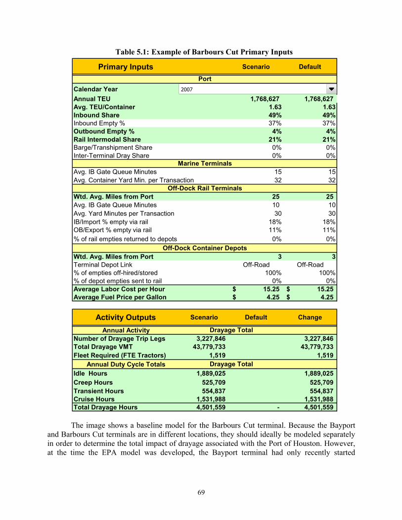
69

Table 5.1: Example of Barbours Cut Primary Inputs

The image shows a baseline model for the Barbours Cut terminal. Because the Bayport

and Barbours Cut terminals are in different locations, they should ideally be modeled separately in order to determine the total impact of drayage associated with the Port of Houston. However, at the time the EPA model was developed, the Bayport terminal had only recently started

Primary Inputs Scenario Default

Calendar YearAnnual TEU 1,768,627 1,768,627 Avg. TEU/Container 1.63 1.63Inbound Share 49% 49%Inbound Empty % 37% 37%Outbound Empty % 4% 4%Rail Intermodal Share 21% 21%Barge/Transhipment Share 0% 0%Inter-Terminal Dray Share 0% 0%

Avg. IB Gate Queue Minutes 15 15Avg. Container Yard Min. per Transaction 32 32

Wtd. Avg. Miles from Port 25 25 Avg. IB Gate Queue Minutes 10 10Avg. Yard Minutes per Transaction 30 30IB/Import % empty via rail 18% 18%OB/Export % empty via rail 11% 11%% of rail empties returned to depots 0% 0%

Wtd. Avg. Miles from Port 3 3Terminal Depot Link Off-Road Off-Road% of empties off-hired/stored 100% 100%% of depot empties sent to rail 0% 0%Average Labor Cost per Hour 15.25$ 15.25$ Average Fuel Price per Gallon 4.25$ 4.25$

Annual ActivityNumber of Drayage Trip Legs 3,227,846 3,227,846 Total Drayage VMT 43,779,733 43,779,733 Fleet Required (FTE Tractors) 1,519 1,519

Annual Duty Cycle TotalsIdle Hours 1,889,025 1,889,025 Creep Hours 525,709 525,709 Transient Hours 554,837 554,837 Cruise Hours 1,531,988 1,531,988 Total Drayage Hours 4,501,559 - 4,501,559

Port

Marine Terminals

Off-Dock Rail Terminals

Drayage Total

Default Change

Off-Dock Container Depots

Drayage Total

Activity Outputs Scenario

2007

70

operations and for that reason the total TEU for 2007 was assigned to Barbours Cut.11 Given the proximity of the two terminals and the small percentage of containers handled at Bayport in 2007, the difference in estimation should be small. The model shows the default values for the current situation and the comparative “scenarios” that are generated by changes in the inputs, either in response to specific policies or general economic trends. For this reason, in the initial model result, the “Default” and “Scenario” results are identical. In the base scenario, the model shows that the Houston dray sector produces an estimated 43.8 million VMT on the Houston road network per year. This is sufficient to generate 3.2 million dray “trip legs” that occupy the positions of approximately 1500 drivers. This model assumes that all drivers serving the Port of Houston perform this activity exclusively. In reality, many of the drivers serve multiple destinations such as the rail yards, along with the ports. For this reason, the number of dray drivers registered to serve the Port of Houston will be higher than the number of full time equivalents predicted by the model. Still, the model is instructive in predicting the number of jobs that would be created by additional TEU at the Port. A cross check on the number of dray drivers associated with the Port of Houston will be possible after the Transportation Workers Identity Credential (TWIC) comes into full force. However, at present the Port of Houston is not scheduled to become fully compliant with TWIC until March of 2009.12

If the TEU volume of the Barbours Cut terminal were to increase by 25 percent to 2.2 million, and all of the other variables were held constant, the model predicts an increase in the VMT generated by the Barbours Cut terminal of 9 million. In addition, an increase such as this could be expected to generate additional gate and yard congestion, which would increase the total number of idling hours generated by the port. If the average queue time were to increase from 15 minutes to 30 minutes, for example, the model predicts that the number of idling hours would increase from 1.89 to 2.32 million. Limiting idling is important due to its potential impact on air quality, to be discussed in the next section, but also on the productivity of trucks and drivers involved in drayage.

The dray cycle is split into two distinct types of work: driving and waiting. The first category requires a high level of skill, the second category does not. Dray truckers have an obvious interest in increasing the percentage of their day they spend performing specialized work. Furthermore, the data reveals that dispatching firms are able to keep drivers engaged throughout the day. Therefore, the only time drivers regularly encounter unavoidable periods of idling is at the terminal gates.

Because the majority of rail deliveries go to inner city rail yards, at distances that are not much closer on average than other destinations, increasing the share of cargo destined for rail in the Houston area would not dramatically decrease the drayage VMT given that drayage refers only the VMT generated within the greater Houston area. A theoretical doubling of the rail intermodal share from the Port of Houston Barbours Cut terminal from 21 percent of the total

11 The model that was constructed for the EPA to model Bayport was more preliminary than the model used for Barbours Cut. This was because at the time the model was being developed, the Bayport facility was very new and did not have sufficient data to establish default values with any confidence. Many of the features of Barbours Cut that were captured in the EPA model would also hold true for Bayport given that both facilities serve a similar set of customers and an analogous hinterland. Bayport is a more modern terminal and, given the absence of capacity constraints at present, has greater flexibility in taking steps to improve the dray efficiency of the system. For example, an on-dock rail system is currently being planned for Bayport that might allow the terminal to be less truck dependent than Barbours Cut at some point in the future. 12 “Planned framework for phased-in COTP zone compliance,” http://www.tsa.gov/assets/pdf/public_compliance_groupings.pdf

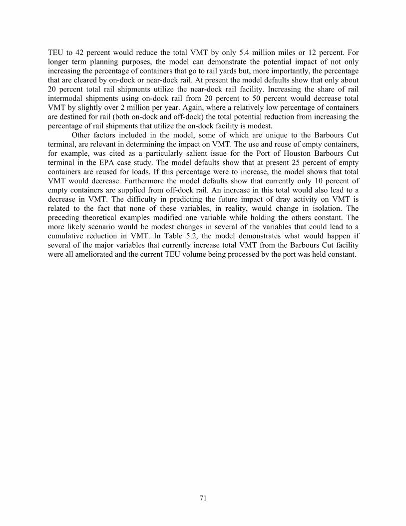
71

TEU to 42 percent would reduce the total VMT by only 5.4 million miles or 12 percent. For longer term planning purposes, the model can demonstrate the potential impact of not only increasing the percentage of containers that go to rail yards but, more importantly, the percentage that are cleared by on-dock or near-dock rail. At present the model defaults show that only about 20 percent total rail shipments utilize the near-dock rail facility. Increasing the share of rail intermodal shipments using on-dock rail from 20 percent to 50 percent would decrease total VMT by slightly over 2 million per year. Again, where a relatively low percentage of containers are destined for rail (both on-dock and off-dock) the total potential reduction from increasing the percentage of rail shipments that utilize the on-dock facility is modest.

Other factors included in the model, some of which are unique to the Barbours Cut terminal, are relevant in determining the impact on VMT. The use and reuse of empty containers, for example, was cited as a particularly salient issue for the Port of Houston Barbours Cut terminal in the EPA case study. The model defaults show that at present 25 percent of empty containers are reused for loads. If this percentage were to increase, the model shows that total VMT would decrease. Furthermore the model defaults show that currently only 10 percent of empty containers are supplied from off-dock rail. An increase in this total would also lead to a decrease in VMT. The difficulty in predicting the future impact of dray activity on VMT is related to the fact that none of these variables, in reality, would change in isolation. The preceding theoretical examples modified one variable while holding the others constant. The more likely scenario would be modest changes in several of the variables that could lead to a cumulative reduction in VMT. In Table 5.2, the model demonstrates what would happen if several of the major variables that currently increase total VMT from the Barbours Cut facility were all ameliorated and the current TEU volume being processed by the port was held constant.

72

Table 5.2: DrayFLEET Beta Version: Houston—Barbours Cuts 2007, 5/11/08

In this example several of the variables have been changed simultaneously. The average

TEU per container has been increased from 1.63 to 1.85. The rail intermodal share has increased from 21 percent to 33 percent and instead of 20 percent of the rail cleared by an on-dock facility, this percentage has increased to 50 percent. While barge transshipment played no role in the old model, in the new scenario barge transshipment now accounts for 15 percent of containers cleared by the Barbours Cut terminal. The average distance to off-dock rail terminals has decreased from 25 miles to 20 miles, indicating the opening of one additional off-dock terminal located in closer proximity to the port. Furthermore the destination of container consignees has been reduced from an average of 40 miles from the port to 25 miles, indicating a change in land use that would place a greater number of receivers nearer to the port. Finally, the percentage of empties reused for loads and the percentage of empties supplied by off-dock rail have both been increased. The cumulative impact of summing all of these changes on total dray VMT is quite significant. Under the assumptions of this model, total VMT generated by the Barbours Cut facility would drop by more than half to slightly less than 20 million miles per year. This could be dubbed a best case scenario for Barbours Cut. The question remains, however: even if many modest steps were taken to improve the dray efficiency at Barbours Cut, would those steps be sufficient to offset the projected growth in volume for the near future?

5.2 Emissions The EPA model can also be used to assess the cumulative emissions impact of dray

activity on air quality. More inputs are required to model the emissions impacts when compared

Primary Inputs Scenario Default Scenario Default

Calendar Year Wtd. Avg. Miles from Port 25 40Annual TEU 1,768,627 1,768,627 Weighted Avg. Crosstown Miles 15 20Avg. TEU/Container 1.85 1.63 % of empties supplied from off-dock depots 0% 0%Inbound Share 49% 49% % of empties returned to off-dock depots 0% 0%Inbound Empty % 37% 37% % of empties reused for loads 40% 25%Outbound Empty % 4% 4% % of empties supplied from off-dock rail 20% 10%Rail Intermodal Share 33% 21% % of empties returned to off-dock rail 1% 1%Barge/Transhipment Share 15% 0%Inter-Terminal Dray Share 0% 0% Wtd. Avg. Miles from Port 2 2

Export Tons Trucked 0 0Avg. IB Gate Queue Minutes 15 15 Avg. Export Tons per truck 20 20Avg. Container Yard Min. per Transaction 32 32 Import Tons Trucked 0 0

Avg. Import Tons per truck 20 20Wtd. Avg. Miles from Port 20 25 Avg. IB Gate Queue Minutes 10 10Avg. Yard Minutes per Transaction 30 30 Port/Terminal InitiativesIB/Import % empty via rail 18% 18% 90% 90%OB/Export % empty via rail 11% 11% 50% 20%% of rail empties returned to depots 0% 0% 100% 100%

100% 100%Wtd. Avg. Miles from Port 3 3 70% 70%Terminal Depot Link Off-Road Off-Road 0% 0%% of empties off-hired/stored 100% 100% 100% 100%% of depot empties sent to rail 0% 0% Other (placeholder) 0% 0%Average Labor Cost per Hour 15.25$ 15.25$ Average Fuel Price per Gallon 4.25$ 4.25$

Annual Activity Pollutant (annual tons) Drayage TotalNumber of Drayage Trip Legs 2,213,895 3,227,846 (1,013,952) HC 21 21 Total Drayage VMT 19,421,585 43,779,733 (24,358,148) CO 104 104 Fleet Required (FTE Tractors) 768 1,519 (751) Nox. 438 438

Annual Duty Cycle Totals PM10 11 11 Idle Hours 1,091,961 1,889,025 (797,064) PM2.5 9 9 Creep Hours 295,279 525,709 (230,430) CO2 64,943 64,943 Transient Hours 249,774 554,837 (305,063) Fuel Use and Total CostCruise Hours 638,297 1,531,988 (893,691) Fuel - Gallons 5,804,444 5,804,444 Total Drayage Hours 2,275,311 4,501,559 (2,226,248) Total Drayage Cost 90,614,644$ 90,614,644$

Emissions Outputs

Primary InputsContainer Shippers/Consignees

Initiative Inputs (Preliminary)

Port

Marine Terminals

Scenario Default

Other Port Truck Trips (Optional)

Off-Dock Rail Terminals

Drayage Total

Stacked TerminalOn-Dock RailAutomated Gates

Neutral Chassis Pool

Default

Container Info System (Inactive)Virtual Container Yard

Change

Extended Gate Hours (Inactive)

Change

y

Drayage Total

Off-Dock Container Depots

Drayage Total

Scenario DefaultActivity Outputs Scenario

2010

73

with the VMT. Specifically, in order to estimate the emissions, the EPA required information on the age of the fleet currently in operation at Houston and the activity profile of these trucks, i.e., how much time they spend in free flow speed vs. idling. A third category of activity was included in the model, dubbed creep idling, which refers to the time when a truck is in queue with its engine running and “creeping” to the front of the line in order to receive service.

CTR provided the EPA with the baseline fleet profile for the Houston dray fleet used in the model. CTR also provided estimates as to the average wait time at the gates and truck turn time. The model years were then evaluated according to their emissions performance for both free flow and idling. The fleet profile is illustrated in a chart that, in the model, is entitled “fleet inputs” and is shown in Figure 5.1. Because the default situation is modeled, the default and scenario curves are identical.

Figure 5.1: Houston Dray Fleet Age Distribution

The EPA model provides baselines for several modeled ports and in each case the age profile of the fleet has a strong correlation with the total emissions produced. All of the dray fleets included in the model follow a similar age pattern, yet there are significant distinctions in the age distribution. The Port of Houston fleet was shown to be comparatively newer than the fleet serving the Ports of Los Angeles and Long Beach. Obviously, this profile is a snapshot of a dynamic situation given that the Ports of Los Angeles and Long Beach are taking significant steps to retire the oldest vehicles serving the port, including a mandatory retirement schedule that will begin later this year. A comparison chart shown in Figure 5.2 demonstrates the distinction between the Houston dray fleet (Scenario) and the fleet from Los Angeles (Default) at the time the baseline research for the EPA model was performed.

-2.0%0.0%2.0%4.0%6.0%8.0%

10.0%12.0%14.0%16.0%18.0%

0 1 2 3 4 5 6 7 8 9 10 11 12 13 14 15 16 17 18 19 20 21 22 23 24 25 26

%

Age

Age Distribution Curves

Scenario

Default

74

Figure 5.2: Comparison of Age Distribution Curves for Houston (Scenario) and Los Angeles

(Default) dray fleets

As can be seen, the relative “peaks and valleys” of the distribution are similar, yet the population of trucks from the Los Angeles sample has a higher proportion that are more than 13 years of age.

This truck profile is then run through a model that weights the total VMT and time spent idling. The result is an estimate of the major pollutants produced by dray activity in Houston. Using the default inputs, the model shows the following cumulative air emissions impacts (Table 5.3) for the Barbours Cut terminal, at a TEU volume of 1.77 million per year.

Table 5.3: Outputs of EPA Drayage Model for Major Pollutants produced by Dray Activity In Houston (Default Scenario)

Emissions Outputs Scenario Default Change

Pollutant (annual tons) Drayage Total HC 53 53 CO 251 251 Nox. 1,327 1,327 PM10 31 31 PM2.5 26 26 CO2 144,301 144,301 Fuel Use and Total Cost Drayage Total Fuel - Gallons 12,897,349 12,897,349 Total Drayage Cost $ 179,126,803 $ 179,126,803

Given Houston’s non-attainment status for ozone, the first areas of potential concern in

assessing the emissions impacts of dray activity are the ozone precursors: Oxides of Nitrogen (NOX) and Hydrocarbons (HCs), resulting from incomplete combustion and/or evaporation, which further results in the formation of ground level Ozone (O3). Many of the strategies

-2.00%0.00%2.00%4.00%6.00%8.00%

10.00%12.00%14.00%16.00%18.00%

0 1 2 3 4 5 6 7 8 9 10 11 12 13 14 15 16 17 18 19 20 21 22 23 24 25 26

%

Age

Age Distribution Curves

Scenario

Default

75

outlined in this report that reduce either dray trips and VMT, idling, or creep idling will have a positive and cumulative impact on air quality.

5.2.1 Improving the TEU-to-Container Ratio The model estimates that improving the TEU-to-container ratio from 1.63 to 1.85—i.e.,

bringing it in line with ports on the Pacific Coast—would reduce emissions by a substantial margin (Table 5.4).

Table 5.4: Impact of improved TEU to container ratio

5.2.2 Comparison: Reduction in Truck Turn Time and Gate Queuing If the average gate queuing time at the Barbours Cut container terminal was reduced by

50 percent and all other metrics were held constant, the model estimates that the impact on major emissions from the reduction in idling would be as shown in Table 5.5.

Table 5.5: Impacts of Reduction in Gate Queuing Time

As can be seen, even a substantial reduction in the queuing and idling time at the Port of

Houston Barbours Cut terminal would have a relatively modest impact on the total pollution emissions, particularly when compared with the improvement of the TEU-to-container ratio mentioned previously. On the other hand, delay and processing speed at the container terminal is

Pollutant (annual tons) Drayage TotalHC 47 53 (6) CO 223 251 (29) Nox. 1,176 1,327 (151) PM10 28 31 (4) PM2.5 23 26 (3) CO2 127,812 144,301 (16,490) Fuel Use and Total CostFuel - Gallons 11,423,538 12,897,349 (1,473,811) Total Drayage Cost 158,721,247$ 179,126,803$ (20,405,557)$

Emissions Outputs Change

Drayage Total

Scenario Default

Pollutant (annual tons) Drayage TotalHC 52 53 (1) CO 245 251 (6) Nox. 1,307 1,327 (21) PM10 31 31 (0) PM2.5 26 26 (0) CO2 142,224 144,301 (2,078) Fuel Use and Total CostFuel - Gallons 12,711,665 12,897,349 (185,684) Total Drayage Cost 168,975,122$ 179,126,803$ (10,151,681)$

Emissions Outputs Change

Drayage Total

Scenario Default

76

a metric that the Port of Houston has direct control over and has in fact already been assertively addressed in the past while the ratio of the 20-ft to 40-ft containers is a function of the markets the Port of Houston currently serves. Trucking firms report that the gate congestion at the Port of Houston has improved in the last few years; therefore, it appears that with regard to reducing gate congestion, most of the low hanging fruit may have already been picked. At present, the majority of the 20-ft containers that move through Houston are tied to European or South American trade as opposed to Asian trade. An increase in the percentage of trade emanating from Asia may lead to a higher TEU-to-container ratio; however, this will be a side effect of a historical change.

5.2.3 Fleet Profile: Impacts of Modernization This report has included discussion of the implications of the age of the drayage fleet. It

has been established that while the Houston fleet is not quite as old as the fleet at Los Angeles, relatively few of the trucks in either location have modern pollution controls. Under a recently passed California mandate, all dray trucks serving California Ports would eventually have to meet 2007 EPA-certified engine requirements. This mandate will impact the Ports of Los Angeles, Long Beach, and Oakland. The EPA model can be used to show what the impact of such a requirement might have on the fleet serving the Barbours Cut Terminal. In the following theoretical example, all trucks serving Houston are shifted from their current age profile to 2007 standards. No other metrics have been changed. Table 5.6 compares dray emissions of an existing default fleet (2006 values) with a theoretical fleet in which all trucks are 2007 certified (Scenario). TEUs, VMT, and operational patterns have been held constant.

Table 5.6: Impact of Shifting Fleet to 2007 Engines


Pollutant (annual tons) Drayage Total HC 24 53 (29)CO 21 251 (230)Nox. 275 1,327 (1,053)PM10 6 31 (25)

PM2.5 3 26 (23)CO2 158,814 158,814

The decrease in criteria pollutants with a 2007 fleet is dramatic. NOx emissions are less

than one-fourth of the current engine fleet’s. Carbon monoxide is less than one-tenth. In recent years, the Texas emissions reduction plan (TERP) has been paying on average $5,296 per ton to reduce NOx from on-road sources. By this logic the value of the reduction in NOx alone could be valued at $5,576,688 in current dollars per year. It is also notable that, according to the model, altering the fleet composition has no measurable impact on fuel efficiency. The researchers believe that some impact on fuel efficiency would likely be realized from a modernization of the dray fleet. However, this is based on the assumption that new vehicles acquired specifically for drayage would have engine profiles and cab configurations that would be better suited to dray activity. Therefore, it would not be an “apples to apples” comparison of the same truck makes

77

and models with a different model year, but a different series of trucks that are distinct from the type of trucks used at the Port of Houston currently. These distinctions could possibly be accounted for in a future version of the model.

5.2.4 Combining Fleet Modernization with Operational Improvements The air quality gains that could be achieved from replacing the current fleet with a

modern fleet would be compounded if they could be combined with operational improvements. In order to demonstrate this, the researchers have taken the “best case” operational scenario for Barbours Cut developed in the previous section in which delays were reduced, alternative modes were used and dray distances were shortened, and combined it with the assumption that this new, more streamlined system would be performed using 2007 trucks. The resultant air emissions reductions, according to the model, are reported here.

Table 5.7 thus illustrates the hypothetical scenario in which fleet modernization is combined with wide-ranging operational improvements to minimize dray impacts.

Table 5.7: Scenario with Fleet Modernization Combined with Operational Improvements


Pollutant (annual tons) Drayage Total HC 11 53 (42)CO 10 251 (241)Nox. 21 1,327 (1,306)PM10 3 31 (28)PM2.5 1 26 (25)CO2 71,051 144,301 (73,250)

In this scenario, the total VMT is reduced from 43.8 million to 19.4 million, the number

of hours spent idling or creep idling is reduced, and drayage is performed with best available technology (BAT). If all of these actions are taken, dramatic reductions in dray air quality impacts are possible. It should also be noted that these changes do not run counter to the real world constraints and orientation of the Barbours Cut terminal, which is and will always be a truck-oriented terminal. In other words, it does not transform the orientation of Barbours Cut into a rail-driven port such as the Port of Tacoma, where the majority of containers are cleared by rail. Furthermore, this model does not introduce any new technologies such as hybrid trucks, which may play some role in the dray fleet in the future. It also does not introduce alternative fuels, such as liquefied natural gas, that are being seriously evaluated in Southern California and may reduce the totals for certain pollutants.13

5.3 Dray Impacts on Traffic The cumulative VMT produced by the dray sector serving the Barbours Cut terminal has

been assessed; however, when and where this VMT is generated is as important as the amount that is generated. The City of Houston faces significant congestion problems that impact many areas of the network. However, not all corridors within Houston are excessively congested. On 13 Trucking to the Port, Traffic World, 8 September 2008, 1209 words, Stephanie Nall

78

the less densely populated eastern side of the city, several corridors do not experience regularly occurring heavy congestion. Much of the dray activity in the Houston area is concentrated on corridors that, while not entirely free of congestion, are not among the most congested segments of roadway within the city.

In an attempt to quantify the impact of drayage operations on congestion, a level of service (LOS) analysis was undertaken for the Port of Houston. SH 225 and SH 146 are two important freeways for drayage operations serving rail and container terminals in the Port of Houston. The LOS analysis considered baseline conditions and altered the truck traffic volumes to show the effects that drayage vehicles have on hourly flow rates and traffic density. This guide describes the methodology and identifies data sources for the inputs needed to determine level of service.

The main data inputs needed to calculate LOS are speed, traffic counts (AADT and truck AADT), and the physical characteristics of the roadway. These inputs are used to calculate free flow speed and the hourly flow rate adjusted for the changes in traffic flow over an hour, presence of trucks, number of lanes, and driver population.

5.3.1 Study Freeways: SH 146 and SH 225 The two study freeways were SH 146 and SH 225 because of the high volume of

container carrying trucks that travel on these roadways. Freeway segments analyzed were determined according to their proximity to the port and data availability. Segments that are known to handle large volumes of drayage vehicles were included. The limiting factor in the freeway analysis and length of study segment was truck data on annual average daily traffic (AADT). Aerial photos and overall AADT was available at more locations than was truck AADT. Truck AADT data was collected using paper maps provided by TxDOT’s Transportation Planning and Programming Division. Overall AADT was available through the GIS online statewide planning map.14

The freeway segments analyzed for SH 146 are from Spur 330 to Fairmont South Parkway. The freeway segments for SH 225 went from Scarborough Road east of the intersection of SH 225 and IH 610 to just east of the intersection of SH 225 and SH 134. Data was available for six locations for SH 146 in 2005, five locations for SH 146 in 2006, and at three locations for SH 225 in both years. The locations for AADT data on both freeways are in Table 5.8 and Table 5.9. Figure 5.3 and Figure 5.4 show the freeways, and the location where both AADT and truck AADT data were available is encircled.

14 The URL for the statewide planning map is: www.dot.state.tx.us/services/transportation_planning_and_programming/statewide_planning_map.htm.

LocatN of SS of SWyomMissoFred HFairm

LocEastRailScar

T

not availused for t

tion Spur 330 Spur 330 ming ouri/146E Hartman Bri

mont South P

cation t of SH 134 l Road Streerborough

The number oable for the the 2006 LO

dge South arkway

Lanes4

t 4 4

of lanes for analysis. Th

OS analysis.

F

Table 5.8:

Lanes3 3 3 3 3 2

Table 5.9: 2005 A

76,193,3

122,3

each freewahe same perc

Figure 5.3: SH

79

SH 146 AA

2005 AAD40,36051,23046,89047,86059,58037,400

SH 225 AAAADT 20150 390 340

ay is in one centage of tru

H 146 AADT

ADT Data

DT2005

Vo111162

ADT Data 05 Truck A

6,442 7,771 9,704

direction. Tuck traffic to

T Locations

5 Truck olume ,795 ,795 ,203 ,203 ,017 ,797

AADT 20

The 2006 truo overall AA

2006 AAD44,000

NA 47,00044,00061,00041,000

006 AADT 80,000 98,000

114,000

ck volumes ADT in 2005

DT

were 5 was

5

Step 1. D

Tvolume measuremwas detecharts. Th

Step 2. C

Tfactor (PH

Tlower PH146 beca

15 The URL

.3.2 Baselin

Determine fre

The free flowconditions ments or an ermined for he FFS for S

Calculate flow

The formula HF), numbe

The PHF typHFs. Urban rause the SH 2

L for the speed

F

ne LOS Ana

ee flow speed

w speed (FFor during oestimation this analysi

SH 225 and

w rate (pc/hr

for flow ratr of lanes (N

pically rangeroadways ha225 study se

d chart is traffic

Figure 5.4: SH

alysis

d.

S) is the meoff-peak trathat consides using fieldSH 146 was

r/ln).

te, vp, dividN), heavy veh

vp = V/ (P

es from .8 tave higher Pegments are i

PHF fo

c.houstontranst

80

H 225 AADT

ean speed ofavel times. ers the physd data avail estimated to

des the desighicle factor (

PHF * N * fHV

to .95. RuraPHFs. The Pin more urba

or SH 225 = .

tar.org/speedch

T Locations

f passenger FFS can bical characteable from tho be 65 mph

gn hourly vo(fHV), and th

V * fP)

al freeways PHF was setan condition

92

harts.

cars during e determineeristics of thhe Houston

h.

olume (V) bhe driver pop

or off-peak t higher for

ns.

low to moded through he roadway.Transtar15 s

by the peak pulation (fP).

conditions SH 225 tha

derate field

. FFS speed

hour

have n SH

81

PHF for SH 146 = .90

The number of lanes for the study segments was determined through Google Earth images.

The heavy vehicle factor is calculated using a formula in the Highway Capacity Manual.

fHV = 1/ (1 + Pt(ET-1))

Pt = percentage of trucks (truck AADT/total AADT) Et = 1.5 for level terrain

The truck AADT was found using traffic count maps provided by TxDOT Planning and

Programming Division. The AADT was found using the online TxDOT Statewide Planning Map.

The driver population factor was set to equal one because users of SH 225 and SH 146 are assumed to be familiar users. The hourly volume (V) is also the design hourly volume (DDHV). The traffic counts are AADT values and need to be converted to design hourly volume to perform level of service analysis.

DDHV = AADT * K * D

K = .09 D = .55 (directional split)

AADT = provided by online TxDOT maps The calculated vp is compared against Exhibit 23-2 in the Highway Capacity Manual to

determine level of service. Then, density (pc/mi/ln) is calculated by dividing the flow rate, vp, by the average speed.

5.3.3 Measuring Drayage Impact Two methods were developed for this analysis to measure the drayage impacts on traffic

density. The baseline scenario for each method assumes that drayage vehicles do not use SH 146 or SH 225 at the AADT locations. Four other scenarios were evaluated that assume drayage traffic constitutes 25 percent, 50 percent, 75 percent, and 85 percent of the total truck AADT. This percentage of the truck traffic was removed from the truck AADT to evaluate how overall AADT and traffic density changes when drayage vehicles are no longer operating on SH 146 or SH 225.

Method 1: Remove Percentage of Drayage Vehicles

Method 1 adjusted the truck AADT by removing the percentage of drayage vehicles depending on the scenarios described above. This method assumes that latent demand from passenger vehicles exists for SH 146 and SH 225 and replaces the drayage trucks with an equivalent number of passenger vehicles. AADT will increase because 1.5 cars replace every drayage truck removed from the system. The passenger-car equivalents for trucks are 1.5 for level freeways, which was assumed for these study corridors (Highway Capacity Manual 2000, Exhibit 23-8). Using this method, the traffic density is constant for all five scenarios, so only

82

traffic density value was provided for the Method 1 tables. Appendix C shows how AADT increased while truck AADT decreased on SH 146 and SH 225 using Method 1.

Method 2: Remove Drayage Trucks, Adjust AADT

Method 2 adjusted the truck AADT by removing the percentage of drayage vehicles and decreased the overall AADT by the number of trucks removed from the system because latent demand is not assumed. Traffic density will change more substantially for Method 2 versus Method 1. Step 1. Remove dray trucks.

New truck AADT = Truck AADT – Truck AADT * Assumed Drayage Truck Percentage

Step 2. Adjust overall AADT.

New AADT = Original AADT – (Original Truck AADT – New Truck AADT)

Step 3. Calculate flow rate with adjusted percentage of trucks, Pt, and DDHV.

5.3.4 Results

SH 146 Analysis

Traffic density increased on SH 146 at Spur 330, Fred Hartman Bridge, and Fairmont South Pkwy while decreasing at Wyoming and Missouri/146E between 2005 and 2006. The level of service was B at all locations in 2005 and 2006 except at Fred Hartman Bridge in 2006. In 2006 using Method 2, a 25 percent reduction in truck traffic assumed to be drayage vehicles in Method 1 caused the level of service to return to B at Fred Hartman Bridge. In Method 2, the presence of trucks has greater impact evident by the traffic densities being lower for the same AADT location and year compared to Method 1 where traffic density is constant. The difference between the methods did not cause level of service ratings to change from LOS B to LOS A even when 85 percent of assumed drayage trucks were removed from SH 146. Tables 5.10, 5.11, and 5.12 provide the results.

Table 5.10: SH 146 - Method 1 (2005 and 2006)

Location 2005 2006

pc/mi/ln LOS pc/mi/ln LOS North of Spur 330 11.64 B 12.69 B South of Spur 330 14.70 B NA NA Wyoming 13.40 B 13.43 B Missouri/146E 13.67 B 12.57 B Fred Hartman Bridge 17.65 B 18.07 C Fairmont South Pkwy 16.41 B 17.99 B

83

Table 5.11: SH 146 - Method 2 (2005)

Location No Dray 25% dray 50% dray 75% dray 85% dray

pc/mi/ln LOS pc/mi/ln LOS pc/mi/ln LOS pc/mi/ln LOS pc/mi/ln LOSN of Spur 330 11.64 B 11.45 B 11.26 B 11.07 B 10.99 BS of Spur 330 14.70 B 14.51 B 14.32 B 14.13 B 14.06 BWyoming 13.40 B 13.27 B 13.14 B 13.01 B 12.96 BMissouri/146E 13.67 B 13.54 B 13.41 B 13.29 B 13.24 BFred Hartman Bridge 17.65 B 17.02 B 16.38 B 15.74 B 15.49 BFairmont South Pkwy 16.41 B 15.97 B 15.53 B 15.08 B 14.91 B

Table 5.12: SH 146 - Method 2 (2006)


pc/mi/ln LOS pc/mi/ln LOS pc/mi/ln LOS pc/mi/ln LOS pc/mi/ln LOSN of Spur 330 12.69 B 12.48 B 12.27 B 12.07 B 11.98 B Wyoming 13.43 B 13.30 B 13.17 B 13.04 B 12.99 B Missouri/146E 12.57 B 12.45 B 12.33 B 12.22 B 12.17 B Fred Hartman Bridge 18.07 C 17.42 B 16.77 B 16.12 B 15.86 B Fairmont South Pkwy 17.99 B 17.51 B 17.02 B 16.54 B 16.34 B

SH 225 Analysis

The LOS analysis indicates that SH 225 has higher traffic densities than SH 146. The Rail Road Street location had LOS C in both years. The results for Scarborough were LOS D in 2005 but improved to LOS C in 2006. Removing drayage vehicles from SH 225 led to more changes in LOS than for SH 146 when using Method 2. The LOS east of SH 134 was B for all Method 2 scenarios. In 2005 at Rail Road Street, LOS C was determined for the base case scenario, and the LOS improved to B when 25 percent of trucks assumed to be drayage vehicles were removed from this data location. Removing greater percentages of assumed drayage vehicles did not lead to enough decrease in traffic density to reach LOS A. In 2006 at Rail Road Street, more assumed drayage trucks had to be removed from SH 225 at this location to reach LOS B than in 2005. Seventy-five percent of assumed drayage trucks had to be removed to reach LOS B. The Scarborough location showed little impact on LOS due to removing drayage trucks from SH 225 at this location. The LOS improved from D to C in 2005, but the LOS did not change in 2006 from assuming that a greater percentage of the trucks were drayage vehicles and removing them from SH 225. Tables 5.13, 5.14, and 5.15 provide the results for Method 1 and Method 2 analyses.

84

Table 5.13: SH 225 - Method 1 (2005)

Location 2005 2006

pc/mi/ln LOS pc/mi/ln LOS E. of SH 134 16.43 B 17.26 B Rail Road St. 20.13 C 21.12 C Scarborough 26.32 D 24.53 C

Table 5.14: SH 225 - Method 2 (2005)


pc/mi/ln LOS pc/mi/ln LOS pc/mi/ln LOS pc/mi/ln LOS pc/mi/ln LOSE. of SH 134 16.43 B 15.82 B 15.63 B 15.44 B 15.36 B Rail Road St. 20.13 C 19.36 B 19.27 B 19.18 B 19.15 B Scarborough 26.32 D 25.35 C 25.26 C 25.17 C 25.14 C

Table 5.15: SH 225 - Method 2 (2006)


pc/mi/ln LOS pc/mi/ln LOS pc/mi/ln LOS pc/mi/ln LOS pc/mi/ln LOSE. of SH 134 17.26 B 16.73 B 16.21 B 15.68 B 15.47 B Rail Road St. 21.12 C 20.49 C 19.86 C 19.23 B 18.97 B Scarborough 24.53 C 23.83 C 23.12 C 22.42 C 22.14 C

Further analysis data for truck volumes on SH 146 and SH 225 (methods 1 and 2) are provided in Appendix C.

5.4 Concluding Remarks The DrayFLEET model was used to predict a number of potential future market

conditions at both Barbours Cut and Bayport terminals. It provides insights into likely scenarios in terms of VMT and emissions, which are useful as policies of the type contemplated in Southern California are evaluated for relevance in Texas. It is also likely that the model can be further calibrated for Houston operations, which will improve its relevance in planning terms. The level of service analysis shows that dray vehicles working the Port of Houston terminals rarely create congestion over the Houston network, although dray truck volumes concentrate on the network links near the terminals at certain times of day. The potential to use rail on and near dock services at Bayport in the future suggest that there may be time to introduce a variety of measures—rather than one single program—to ensure that dray operations are able to match the predicted demand from future container business while addressing social concerns. The next chapter examines a variety of initiatives to mitigate the adverse impacts associated with dray operations.

85

Chapter 6. Potential Mitigation Measures

The objective of this chapter is to identify and discuss potential mitigation options to reduce the impacts of the drayage sector to ensure that drayage activity does not adversely impact surrounding communities. The research team discusses the identified mitigation measures in the following four broad categories of initiatives:

• improve terminal operations,

• modernize (i.e., new technologies) the drayage fleet, and

• divert dray traffic to other modes.

6.1 Initiatives and Policies to Improve Terminal Operations Initiatives to improve terminal operations were examined because air quality and

congestion impacts from a terminal can sometimes be mitigated by improving the efficiency of terminal operations. Long term initiatives such as the Agile Port System demonstration project led by the Center for the Commercial Deployment of Transportation Technologies along with the Port of Tacoma is one example of a strategy to greatly reduce container dwell time and port productivity.16 Boosting terminal efficiency does not always translate to a lessened contribution of dray trucks to urban congestion. In fact, when a terminal becomes more efficient and capable of handling a greater amount of traffic, its total truck traffic can increase due to the impact of latent demand and shippers choosing the port over other alternatives. The researchers have attempted to focus on those changes in terminal operation that have a predictable and measurable effect on dray impacts. In short, there are three key strategies in the short to medium term that can be effective in reducing the impact of dray related congestion from a container terminal.

1. Shifting to off-peak operation

2. Replacing a portion of truck drayage with an alternative mode that would not compete for road space

3. Reducing the amount of deadheading in the system

6.1.1 Shifting to Off-peak Operation This is a strategy for lowering the aggregate amount of car-dray truck interaction. One of

the key distinctions between dray truck activity and long haul trucking is the fact that dray trucks operate almost exclusively during the work day. The restriction to daytime operation hinders the ability of planners to properly accommodate for growth in dray traffic. Several proposed policy solutions, such as variable time of day tolling, for example, would have limited effectiveness so long as dray trucks are confined to the traditional operating windows of marine container terminals. Even if a container terminal is extremely efficient in turning dray trucks in a timely manner, the impact on the road network need not be improved so long as demand remains fixed within the constraints of limited operating hours. Only if the truck arrivals and departures are

16 “Agile Port System Demonstration: The Efficient Marine Terminal,” Presentation by Jeanne Beckett, AAPA Port Operations, Safety and IT Seminar, April 25, 2007 http://aapa.files.cms-plus.com/SeminarPresentations/07_OPSAFIT_Beckett_Jeanne.pdf

86

spread out over a longer period can a reduction in the peak period road consumption of dray trucks be realized.

Extending the operating hours of a container terminal, particularly a marine container terminal, is an expensive and potentially risky proposition. Several container ports surveyed in the course of this study have experimented with extended operating hours in the past only to abandon the policy due to high costs and insufficient demand.

Extending the gate hours is not an end unto itself. Rather, it is only valuable to the extent that the terminal is actually able to attract a significant share of transactions during the off-peak hours. The attempt to meet these two conditions of extending hours and stimulating the market for off-peak delivery simultaneously was one of the key innovations of the California Pierpass Initiative. The challenges of extending gate operations grow significantly if the terminal provides non-grounded stacked services, as this entails the use of longshore labor beyond the normal working day, which can contribute significantly to cost. None of the three major marine container terminals operating in Texas currently has extended gate hours. Both the Barbours Cut and the new Bayport terminal at the Port of Houston have operating hours of 7:00 a.m. to 5:00 p.m. Monday through Friday or 45 operating hours per week. The Maersk terminal at Barbours Cut has slightly longer posted gate hours, from 7:00 a.m. until 6:00 p.m. Monday through Friday. The terminal, however, enforces terminal entrance cut-off times for import loads if they are already on a wheeled chassis at 5:00 p.m. and if they are grounded at 4:45. Other times for APM terminals around the country are shown in Table 6.1. As can be seen, off-peak hours are still a rarity for APM terminals, even those that are much larger in terms of area and throughput.

Gate Hour Trends at Other Terminals around the Country

It should also be noted that Houston is not the only city that has a large container port impacting patterns of road usage. In cities such as Oakland, which has a higher TEU volume and worse congestion as measured by total hours of delay than Houston, no extended gate hours have been permanently adopted. Oakland first experimented with extended gate hours in 2005, allowing export loads to be delivered to one of the Port’s eight terminals Monday through Friday until 2:30 a.m. The exclusion of import loads from the program allowed the port to avoid the extensive use of gantry cranes during the night hours. The Oakland program of extended gate hours ran from September until December 2005 in an attempt to better serve shippers of agricultural products. Having set a goal of 300 transactions per night, the program achieved on average 150 transactions per night and was considered a modest success but did not achieve “the critical mass” sufficient to continue past the trial period. It was hoped that the program would be sufficient to give truckers one more turn during the day, thereby increasing the percentage of truckers who were able to make a profit. In general, the Port of Oakland found that the underperformance of the night gate was tied to resistance by drivers to drive at night if they received no additional compensation above and beyond the compensation for a normal delivery. It may be that the Port overestimated the percentage of truckers who needed an extra turn to remain profitable. In addition, while many warehouses were open later than the port gates, many others kept a standard work day. The SSA gate was picked because it served the majority of the agricultural customers who were expected to take advantage of 24 hour operation. The Port of Oakland officials reported that one of the key distinctions between the success of the extended gate hours at Southern California ports and the underwhelming performance of Oakland is the fact that Oakland does not have the capacity constraints that were present in Southern California.

87

In a report of the port commissioners, Ray Kidd stated that truckers “will not” use night gates in significant numbers without some type of financial penalty for using the daytime.17

Table 6.1: Summary of APM Terminal Hours

Terminal Area (acres) Cranes Berth

Monday-Friday Gate

Hours

Weekend hours

Port's total 2006

TEU Volume (Marad)

Hours of Congestion

Charleston 107 10 3,803 ft 8-4:30 (closed for lunch) 1493285

Houston 104 3 2,000 ft 7-6:00 1268163 56

Jacksonville 60 8 1,700 ft 7-4:30

151827

Los Angeles 484 14 7,190 ft 7:00 a.m.–2:30

a.m. Saturday 7-5 5633665 72

Miami 72 12 5,000 ft 7–4:30 743355 50

Oakland 148 8 3,200 ft 7–5:00

1399967 60

Port Elizabeth 350 11 6,001 ft 6–4:30 n/a 46

Tacoma 135 5 2,200 ft

8–4:30 Wednesday

and Friday 6-10PM,

Saturday

Saturday 8-12 1091934 45

Virginia 600 6 3,205 ft

7–5:00 1409732

(Norfolk) 30

Savannah (Multi-user

facility) 1208 21 7–6, cutoff for

inbound at 4:30 1580925

The Port of Oakland confirmed that since the failure of the 2005 pilot program, the port

has not tried another pilot program and has instead focused on funding technology improvements. It should be noted that, as a landlord port, the Port must rely on the terminal operators to finance such initiatives. In the 2005 case, SSA agreed to leave the gates open for an extended hours at the request of its shippers. To the extent that the costs of the extended gate hours exceeded the benefits to shippers, this difference was financed by SSA.18

It should be noted that the truck-related congestion encountered at Houston is not unique. Most of the container terminals around the country are located in or near cities that have pre-existing congestion problems that would seem to act as an incentive to lengthen gate hours. The following bullets highlight some of the decisions regarding gate hours that were recently implemented at terminals around the country.

17 Audio Presentation to maritime committee regarding extended gate hours pilot program, January 19, 2006. www.portofoakland.com 18 Interview with Tim Leong, Environmental Scientist at the Port of Oakland, July 18, 2008.

88

• In Seattle, Eagle Terminals, which along with SSA and MTC runs a container terminal at the Port of Seattle, has reduced its hours of gate operation from closing at 6:00 p.m. to 5:00 p.m. The change took effect on April 28, 2008, and was taken, according to an official at Eagle, as a cost-cutting measure. At the Port of Tacoma’s terminal run by APM, gate hours have recently been extended to 10:00 p.m. for Wednesday and Friday to handle elevated demand. No swap service is provided for nighttime operations.19

• At the Port of Charleston South Carolina’s public port authority, the terminals operate during normal business hours between 7:00 a.m. and 5:30 p.m.; however, the terminals do work through lunch.20 The port handled 1.5 million TEUs in 2006.

• At Boston’s Conley Marine terminal, the hours of terminal operation are 7:00 a.m. to 5:00 p.m. The Port handled only 139,000 TEUs in 2006.21

• Virginia International Terminals, Inc. controls four separate terminals and is one of the largest container facilities on the mid-Atlantic with a size slightly larger than that of Houston, handling 2,046,286 TEUs through all terminals in 2006. The gate hours for two terminals, the Norfolk International Terminal (recently expanded) and the Portsmouth Marine Terminal, which is also a container facility, are 6:00 a.m. to 6:00 p.m. Monday through Friday or 60 hours per week. The Virginia Inland Port, which is designated as a terminal for supporting the Port of Virginia, is open from 7:30 a.m. to 4:30 p.m.22

• The Port of Savannah has instituted extended gate hours for Tuesday, Wednesday, and Thursday at its publically controlled Garden City Terminal until 11:30 p.m. These extended hours have helped the port accommodate one of the sharpest gains in TEU throughput in recent years. When queried about the possibility of further expansions of gate hours at their facilities, representatives from the Charleston and Savannah Port authorities expressed confidence that gate hours can be extended when needed without significant problems from the labor community. There is now sufficient experience with extending gate hours, permanently and temporarily, that that ports no longer fear resistance from labor when proposing an extension of gate hours. Rather, this is now seen as a normal policy that can be adopted whenever the benefits exceed the marginal costs.23

In the opinion of several East Coast port officials, when a container terminal considers

extending gate hours, it first does so during the five-day workweek. There is an order of operations based on logistical complexity and cost. Extending hours for one or two nights a week, tied to peak periods for ship arrivals, is a logical first step. If evening hours during the

19 “APM Terminals Tacoma – Hours and Holidays” http://www.apmterminals.com/northamerica/tacoma/terminalinfo.aspx?id=1194 20 “Port of Charleston: Marine Terminals” http://www.port-of-charleston.com/charleston/default.asp 21 “MASSPORT: Conley Terminal” http://www.massport.com/ports/conle_termi.html 22 “Virginia International Terminals” http://www.vit.org/TerminalInfo.aspx 23 Interview by Rob Harrison with Port of Savannah and Charleston Officials at the Virginia Maritime Association Annual Symposium, May 8, 2008.

89

five-day workweek are not sufficient, Saturday and Sunday hours are offered. As evidenced by the Oakland case, restrictions can sometimes be placed on the types of services offered during extended hours.

Could Gate Hours be Extended at Houston?

The characteristics of container operations at the Port of Houston favor the extension of gate hours in certain respects. For example, the Port of Houston is not merely a landlord port but rather operates the majority of the container handling capacity internally. Therefore, the port authority can decide internally whether extended gate hours would benefit the operations of the port and can negotiate directly with the unionized labor force. The fact that Barbours Cut is still running near capacity, which was not the case for the Port of Oakland, also bodes well for the potential of attracting significant usage from an extended gate system. Another “advantage” that Houston has over some other ports is that it has no on-dock rail and a very low percentage of containers cleared by near-dock rail. Jimmy Jamison estimates that in 2007, all rail service from the Port of Houston, including boxes drayed to local rail terminals, constituted no more than 10 percent of the total TEU throughput.24 The dearth of intermodal rail at the Port of Houston means that containers that are less time sensitive and that might be attracted to intermodal rail at another port must be cleared by truck if they arrive at the Port of Houston. Therefore, there is a class of containers for which same day delivery is not as important for which nighttime pickup and delivery may be attractive. The growing role played by import distribution centers in the Houston area, which tend to operate 24/7, is also an advantage. However, according to Jimmy Jamison, a significant share of containerized cargo still moves from terminals, in particular Barbours Cut, to traditional warehouses that, assuming they would maintain those same hours if the port extended its own hours, could not benefit from the expansion of hours.

Clearly, given that the most of the railroad yards in the Houston area operate until late at night and rail operations in general operate on a 24-hour clock, a better matchup between the operational profile of rail and marine ports would be useful. When on-dock rail is an option, the impact of restricted gate hours can be mitigated. However, when each rail move first requires a dray move, the rail yard operation must accommodate itself to the restrictions placed by the marine terminal. Interviews with drivers at Houston’s largest rail yard demonstrated the symbiotic nature of the two facilities with many interviewees at the rail terminal stating that they were either coming directly from the Port of Houston Barbours Cut terminal or were heading there after their delivery. The Englewood terminal is open 24 hours a day, 7 days a week. Operating hours for other Texas rail terminals are listed here.

• Barbours Cut (near dock) intermodal hub: 8:00 a.m. to 5:00 p.m.

• Settegast: Monday–Friday, 5:00 a.m.–9:00 p.m.; Saturday, 7:00 a.m.–5:00 p.m.; Sunday, 7:00 a.m.–3:00 p.m.

• Englewood: 7 days a week, 24 hours a day

• Pearland: Monday–Friday, 5:00 a.m.–10:00 p.m.; Saturday–Sunday, 7:00 a.m.–6:00 p.m.

24 Interview by Nathan Hutson with Jimmy Jamison, Director of Operations at the Port of Houston, September 10, 2008.

90

When compared with the Barbours Cut Container terminal, one factor that may favor the extension of gate hours at Bayport is the less labor intensive gate process (paperwork is sent to a central depository for processing rather than being handled by a single clerk at the gate). It would be possible to receive exports and hold them in a grounded storage area to be worked by a crane the following day. The layout for the Bayport master plan shows a significant share of total dock space dedicated to wheeled container storage.25 The single largest factor in determining whether or not Bayport is ready for extended gate hours, according to Jimmy Jamieson at the Port of Houston, is the nature of the container ship strings that will call this terminal. If the terminal, in the future, handles a high percentage of Asian cargo, this will match up well with 24-hour distribution centers. In this case, the shippers will demand longer hours and be willing to pay for them either directly or indirectly. The first service to call Bayport was an Asian service. However, in the last year a Northern Europe service has also started to call the terminal, which means that at present the cargo mix at Bayport is not substantially different from that of Barbours Cut. In the long run, the Bayport terminal will likely take on a dominant Asian profile while Barbours Cut will retain its traditional European/South American strings. However, the port does not believe these profiles will be truly solidified until the completion of the Panama Canal expansion.

Alternative Strategies for Night Hours

The major cost components of extended gate hours are the operation of yard cranes and the operation of the gates themselves. Of the two elements, the crane operation constitutes a far larger share of the total cost. Jimmy Jamieson at the Port of Houston referred to the actual gate operations as “pennies on the dollar” when compared with the total cost of having the terminal “turned on.” Therefore, a system in which the terminal is not fully functional but is still able to receive certain truck shipments after hours may be an appropriate compromise for terminals transitioning to extended hours that do not have sufficient demand to warrant full scale nighttime operation. A system for processing exports without involving gantries was adopted at Oakland when it started a trial program to handle only exports during a 2005 trial. An export-only operation at Bayport could be run by receiving wheeled containers at night and stacking them the following day. The import process would likely be trickier to accomplish given that it would involve limited use of road cranes at night. For imports, an extended gate operation could work under one of two scenarios. One rubber tired gantry (RTG) could be reserved for yard operations after regular hours. Alternatively, a system could be established where imports could be pre-handled, prior to the driver’s arrival, and loaded onto port-controlled pooled chassis. This system, as envisioned, would require several modifications. First, it would require a “binding appointment system” for afterhours import pickups in which the terminal would know which containers would need to picked up at some point during the evening and would prepare the containers to be picked up from a wheeled storage staging area. The term binding appointment system means that the trucking firm would pay a financial penalty if the scheduled pickup did not occur. It also means that a participating terminal would need sufficient space to set aside what would admittedly be a less efficient use of space for nighttime deliveries. Obviously this is a proposal that would only be workable at terminals that have surplus dock space. At the Barbours Cut Container terminal, a significant share of total dock space is already occupied by wheeled 25 “Bayport Master Plan” http://www.portofhouston.com/pdf/genifo/POHA-BayportMasterPlan.pdf, Available Online, Accessed August 15, 2008.

91

storage due to the high percentage of dangerous and hazardous cargo currently handled by the port.

Another factor that must be considered when evaluating the attractiveness of extended gate hours is the potential light and noise pollution impacts of nighttime crane operations. Again, this is not as much of a factor in terminals with grounded operation and if the extended hours adopted by a terminal were to apply solely to grounded containers, it would not be a large factor. At the Bayport terminal, in particular, nighttime operations from shipside cranes have been a source of community tensions since the terminal’s opening. It is not clear to what extent nighttime operations from gantry cranes serving trucks would add to the overall noise level.

In summary, despite the substantial growth in containerized shipping, many of the largest marine terminals in the country still keep standard daytime hours of 7:00 a.m.–5:00 p.m. The Port of Houston has had limited and informal experience with extended gate hours. In the time prior to the opening of Bayport, the port of Houston would on occasion offer extended gate hours or weekend hours in order to fulfill the demands of major shippers who were unable to clear cargo in a timely fashion otherwise. When Wal-Mart first started shipping Asian cargo directly through Barbour’s Cut, it agreed to compensate the port financially for the extra cost of maintaining an open gate and a crane to handle containers within the yard.

The State of Texas could enact legislation analogous to that passed in California requiring that terminals located in congested areas such as the Barbours Cut container terminal operate at both peak and off-peak hours to allow dray vehicles to make pickup and deliveries at times that are not heavily congested.

Looking further down the line, once longer operating hours for the terminal have been established, Texas could assist in establishing financial incentives for drivers to make deliveries during off-peak hours. This program may or may not be modeled on the Los Angeles/Long Beach PierPASS program. Any system that comprehensively charges a higher rate for dray trucks to access the road network would likely be effective. This could be a container fee or it could be a variable toll levied on the first link of the public road network.

6.1.2 Potential Role for Terminal Appointment System Idling emissions are a key source of air pollution tied to dray activity at terminals in

Texas. Texas could enact a stricter anti-idling standard for trucks operating within the terminal area. The definition of idling could be broadened to include “creep idling” (to include time in which the engine is on but the vehicle is not consistently in gear). This would have the effect of providing a mechanism for penalizing excessive queuing. In order to correct for this, the terminal could set up an appointment system that would service each vehicle, without significant delay, when its turn had arrived. Vehicles that arrived without an appointment or significantly prior to their appointment would be required to wait without idling their engines. Appointment systems are currently used at several terminals in California. The average “slot” time is one hour and slots can be booked up to two weeks in advance.26

Container appointment systems are still in their experimental phase; however, there are several indications that an appointment-based system has the potential to pay dividends both in terms of terminal productivity and with regard to the emissions associated with container terminal operations. When the number of times a dray truck can enter the terminal is constrained,

26 “Planning local container drayage operations given a port access appointment system,” http://www2.isye.gatech.edu/people/faculty/Alan_Erera/pubs/ne06drayage.pdf

92

for example, it may provide an additional incentive for the dispatcher to complete two transactions (one inbound and one outbound) with each appointment slot, thereby lowering the total number of dray trips required.

Marine terminals are not the only terminals that have started using container appointment systems. The Canadian National (CN) now uses a container appointment system at their Toronto and Montreal rail terminals. The appointments are set to either 60-minute or 120-minute windows depending on the time of day with the shorter windows reserved for the busier periods. At present, no CN rail terminals in the United States follow this practice. At the growing CN Memphis terminal, dray firms currently have to specify the day, but not the hour, that the box will be delivered. As opposed to the Southern California ports in which truck appointments were instituted largely in response to the Lowenthal Bill, the CN plan is an industry-led initiative. Thus, the researchers investigated the characteristics of these two rail terminals in Montreal and Toronto to determine why they were chosen for the institution of an appointment system.

The Montreal Terminal is in operation 24 hours a day, 7 days a week. It receives daily train service. The terminal has instituted an expedited service gate, entitled the “speed gate,” which should allow for a higher number of trucks that pass prequalified checks to enter the terminal gate more quickly, thereby lowering the average queue time outside the gate. The following technologies describe some of the prerequisites that have been required to institute this new type of gate.27

“1. Drivers approaching the Speed Gate will pass through a portal where a series of cameras record the condition of the equipment (container and chassis or trailer).

2. The driver proceeds to an automated gatestand where biometric technology validates the driver's identity.

3. The driver inputs the unit initials and number, which are validated by Optical Character Recognition software.

4. The customer's bill of lading is activated. This allows the driver to place the unit for loading to rail.

5. A transaction ticket is issued to the driver at the gatestand.

6. A gate operator monitors the cameras from the terminal office and is available for assistance as required.

7. Speed Gate is operational at CN's Montreal, Edmonton, Winnipeg and Vancouver.”

In Toronto’s Brampton terminal, a restricted container appointment system was put into place in 2005. CN released the following statement regarding the move.

“The arrival patterns at CN Brampton are now such that the inability to manage the volume arriving at the terminal by destination is causing congestion issues. More traffic than can be handled on a daily basis is arriving at the terminal creating terminal inefficiencies and a deteriorating level of service. In order to position CN Brampton intermodal to handle the expected growth in international trade CN is implementing a reservation process for all export traffic (loads and empties) that recognizes destination when providing appointments.”

27 “CN – Speed Gate” http://www.cn.ca/en/shipping-intermodal-terminals-speed-gate.htm

93

At Toronto’s Brampton terminal, CN also recently made the decision to decrease the amount of free time provided to containers being delivered to the terminal. This was done to increase the total terminal capacity and reward customers who clear their cargo in an efficient manner. For some terminals, an appointment system is seen as a less expensive alternative for lowering congestion than extended gate hours.

In determining the number of appointments that can be made available, the terminal must determine the length of the appointment slot. From the perspective of the dray operator, any appointment slot is a potential constraint, yet the difference between a slot that is half an hour, one hour, or two hours may be substantial. If the terminal forces trucks into narrower windows, then it must provide a greater total number of windows to achieve the same utility.

The Lowenthal bill, which took effect in 2002, provides an opportunity to study the divergent strategies that terminals could take to improve terminal efficiency and thereby avoid the punitive fees that would be placed by the legislation from inaction. The term extended gate hours was defined for the purposes of the legislation at 70 or more hours a week. In its attempt to reduce idling, the Lowenthal bill focused principally on idling that occurred outside of the terminal. According to Giuliano, 13 terminals within California responded to the Lowenthal provision, of these 3 were already exempt from making changes because they already operated at 70 gate hours per week. While seven terminals chose to institute an appointment system in response to the law, no terminals moved directly to extended gate hours directly as a result of the legislation.28

In her analysis of the impact of container appointment systems at southern California, Guiliano found that a container appointment system was one of the less effective techniques employed for improving terminal efficiency. Truckers had little incentive to participate in the program given that there was no appreciable gain in turn time. The institution of appointment systems in response to AB 2650 had “no measurable impact” on truck queuing at the port gates. Giuliano refers to the passage of PierPASS, in July 2005, as “essentially the end” of the appointment system experiment.29

Given the cost of longshore labor in California, the smaller terminals with fully grounded operations require lower labor costs—i.e., no longshore labor required to make the move. Therefore, the smaller and less technologically advanced ports oftentimes have an easier time moving to extended gate hours than the larger ports, despite the fact that the larger ports are busier and would seem to be more in need of congestion calming measures.

For container terminals that use appointment systems, it has become clear that not all types of deliveries are equally likely to take advantage of the system. Most appointments are made for “import pickups” (picking up a loaded container), because these transactions are often time sensitive and subject to delays.

Technology Driven Appointment System

The Port of Oakland, which already has a gate appointment system in place, is weighing the universal provision of either an RFID or GPS technology for every vehicle operating at the port. The technology would be provided through a $3.8 million grant that the port estimates would be sufficient to cover the initial capital cost and the first three years of operating costs (monthly data plans). After this point, the trucking firms will be required to cover future 28 “The Terminal Gate Appointment System At The Ports Of Los Angeles And Long Beach: An Assessment,” http://www.metrans.org/nuf/documents/Giuliano_OBrien.pdf 29 Ibid

94

operating and capital replacement costs. The Bay Area world trade center currently favors the use of GPS over RFID because they feel that GPS will provide superior information to truckers and the terminal.30 It will assist the truckers in managing their fleet and researchers in studying truck behavior, but most importantly, it will allow the appointment system to shift from a static appointment system in which truckers must meet pre-assigned delivery windows to a dynamic appointment system in which the terminal will receive advanced notification when the truck is within range of the terminal and will adjust its estimated arrival time appropriately. This new system would have several advantages over a fixed window appointment system. The most significant advantage is that it allows the terminal to be aware of other systemic factors that may delay truck arrivals to the terminal, such as excessive congestion on the surrounding roadways. If, as reported by the port, 2,500 units funded with three years of data plan are provided to the 2,500 identified truckers eligible to serve the Oakland terminal, and these units were acquired at the proposed $3.8 million of funding, it would mean that the average expenditure per unit is $1,500.

The Port of Oakland estimates that the fleet of trucks serving their port is approximately 2500 full time equivalents. Given that there was a 2007 container volume at the Port of Oakland of 2.39 million TEUs, this means that each trucker was responsible for handling approximately 950 TEUs per year. It should be noted that approximately 200,000 TEUs in 2007 were empty imports, most of which would not have left the container terminal. Drayage is particularly important for the Port of Oakland given that it does not have on-dock rail.

Weighing the Advantages of a Standardized RFID or GPS Technology

Providing a universal GPS to the truck fleet serving a port is one strategy for driving down costs. GPS data were collected on a small sample of Houston dray trucks during the first year of the study and the exercise is described in Appendix D. For the proposed system in Oakland, the Port is hoping that by standardizing the technology, it can prevent this add-on from altering the market. The GPS technology that is envisioned for the Port of Oakland will be a black box that is installed within the vehicle so it cannot be tampered with by the driver. Monthly subscriptions would be paid out of the upfront capital funds for the first 3 years. Software would show in which terminals the technologies are being used and the impact on truck turnaround times. The units would include a “Geosensing” capability allowing the port to establish an electronic perimeter and inform port operators whenever a truck crosses into the approach area to the port. 31 The technology would also be used to prevent trucks from entering neighborhoods.32

30 Interview by Nathan Hutson with Elizabeth Viverito, Vice President Bay Area World Trade Center, San Francisco, California, July 10, 2008. 31 Interview with Tim Leong, Environmental Scientist, Port of Oakland, July 18, 2008

The Port is still in the process of issuing an RFP, set to be issued by the end of 2008, for a data integrator that would allow fleet operators and the Port to have the exact same information as to the location of trucks, thereby allowing them to better coordinate action. According to the Port, the detailed RFP will be goal oriented and may avoid the prescription of a particular technology. Another goal to be included in the RFP is that the technological approach has the side impact of ensuring that the port keeps registration data on all equipment entering and exiting. There may be some potential to do this in coordination with TWIC; however, TWIC registration is only useful in keeping track of drivers and should be matched, in the view of the Port, with a separate database that tracks all equipment. This would even include long haul trucks that only make occasional trips to the port. 32 “Truck Management Steering Committee Meetings - Discussions on Clean Truck Program Components,” http://www.portofoakland.com/pdf/ctmp_070827_06.pdf

95

6.2 Initiatives to Modernize the Drayage Fleet When compared with the total population of trucks in an urban area, the drayage fleet is

not particularly large. Due to the fact that a relatively small population of trucks call the same facilities multiple times throughout the day, the investment needed to replace a segment of the drayage fleet, by either public sector or private sector actors is not as high as might be imagined. Modernization of the fleet is inevitable given the passage of cleaner engine mandates in 2003 and 2007 that will eventually work their way into the dray fleet. The question is whether or not metro areas in Texas that are already in non-attainment can wait for the natural turnover of trucks to occur or if the state should actively promote the retirement of older vehicles involved in dray activity. The impact of TWIC and other restrictions placed on dray truckers will likely shrink the total number of trucks serving in the dray fleet due to a reduction in part-time drivers. In other words, while the total number of FTEs required to handle dray activity will increase at both marine and intermodal terminals, it is likely that the actual size of the fleet of vehicles servings these facilities will grow at a slower rate due to a trend toward greater specialization of labor.

The Los Angeles Clean Truck Program, which is one of the boldest dray truck modernization efforts in the country, continues to move forward. On May 15, 2008, Los Angeles Board of Harbor Commissioners officially and unanimously adopted the plan, including the provision to eliminate owner-operators from serving the port by the year 2013.33 New details in the plan reveal how the switch over from owner-drivers to company employees will be structured. By the end of 2009, 20 percent of the drivers must be company employees. The percentage increases until it reaches 100 percent by the end of 2013. The equivalent plan adopted by the Port of Long Beach still contains no such provision to replace owner operators with company drivers although it maintains the same schedule for replacing trucks.

While not as extensive, truck replacement and engine retrofit programs have also been adopted at other ports. The Port of Vancouver, which works in close conjunction with the Ports of Seattle and Tacoma, recently started a truck licensing program to ban old trucks from providing drayage service. While not as rigorous as the program adopted by the San Pedro Bay Ports, the licensing system adopted at the Port of Vancouver bans trucks of model year 1993 and older from accessing the port unless they pass a special emissions test. Trucks older than 1989 must have a retrofit that improves their environmental performance. These regulations went into effect in March of 2008.34

The Port of Oakland started a truck replacement program in 2005 targeting vehicles 1993 and older that provides grants of up to $40,000 toward the purchase of a new truck. The program is currently voluntary. It sets a maximum value of “one ton of NOx plus one ton of ROG plus one-twentieth of a ton of PM over one year” at $14,300 and states that the grant amount cannot equal more than 72 percent of the invoice price.35 This does not mean that projects that do not meet the benefit cost ratio for pollutant reduction are not eligible; simply that the agency will cap the grant amount at this level. Eligible participants must demonstrate that the truck they are seeking to replace has been operated regularly in Oakland port service for at least two years. In

33 “LA Adopts Clean Truck Plan” Traffic World, 16 May 2008, Thomas Gallagher 34 FINAL NOTICE: Environmental Requirements, Vancouver Fraser Port Authority March 1, 2008; http://www.pacificgatewayportal.com/tlsportal/ShowFile.aspx?FileName=Final Notice Environmental Requirements - English 35 “Port of Oakland Truck Replacement Program Guidelines,” http://www.portofoakland.com/pdf/envi_prog_06_2.pdf

96

addition, the applicant must show that the truck was used to haul containers for 400 trips in the Port area in the twelve months prior to the application.

6.3 Initiatives to Divert Dray Traffic to Rail The potential use of alternative modes to handle drayage loads has been another option

for removing dray trucks from the roadway. The two most frequently cited options for such a shift are an on-dock or near-dock rail shuttle that could move containers to distribution centers or rail hubs or, in the case of marine ports, container-carrying barge shuttles. A forthcoming TxDOT report 0-5937 will detail options for shifting container cargo onto barges or other marine vessels for dray competitive movements. The opportunities for realizing this particular modal shift are limited in Texas due the limited origins and destinations accessible by barge. Still, when compared to the construction of new rail infrastructure, the infrastructure requirements to create certain dray competitive container on barge movements, such as the proposed shuttle service linking the Port of Houston with the Cedar Crossing industrial park, are not capital intensive and require only modest improvements in dock space. The first cargo types in Texas that will see modal shift are not containerized commodities but heavy steel coils that currently move between the Port’s city docks and local steel distribution yards. An initiative by Richardson Stevedoring (Richway Cartage), which controls a substantial dray fleet in the Houston area, has already made a modal shift to barge in order to move its product to Cedar Crossing with a lower cost transportation option. Allen Eckardt of Richway Cartage estimates that this short haul steel barge service is already removing some 20,000 dray trips from the Houston road network per year.36

Savings from the shift will likely be realized in the area of pavement preservation, congestion, safety, and air quality. Richardson is also planning to move steel cargo from Monterrey Mexico through the Port of Brownsville and by barge directly to receivers in the Port of Houston. This would allow the removal of heavy steel carrying trucks along roads leading all the way to the border. This would not only remove significant truck congestion from the Houston road network but would also lessen the truck impact to one of its most distant intrastate destinations, one that so far has not seen significant modal shift to rail despite the existence of a UP line connecting Houston to the Brownville area. Osprey lines along with its partner Cedar Crossing Terminal Company opened a barge dock suitable for container operation that will likely remove some volume that would otherwise have been moved by truck.37 In short, while container on barge along with other marine options may have more limited avenues for successful adoption, they are in many cases the least capital intensive and more efficient way to realize mode shift for a dray fleet.

Rail currently supports container traffic moving through the Port of Houston by providing the line haul portion of the journey. With the exception of the small Barbours Cut rail yard, most rail facilities that handle containerized cargo emanating from the Port of Houston are located some distance from the port complex and within the Houston urban core. For this reason, dray trucks are responsible for moving rail cargo from the Port to the rail yards. In 1996, the Port took advantage of $13 million in CMAQ funds to improve the container-carrying capacity of the Barbours Cut yard. A goal of these improvements was to lower the impact of dray trucks serving the Port of Houston, which at that time moved only about 700,000 TEUs per year. A certain degree of momentum to substantially improve the rail system in Houston was stalled by the

36 Interview with Allen Eckhardt, Richway Cartage, August 10, 2008 37 Cedar Port barge terminal opens near Houston Ship Channel, Gulf Shipper, April 21, 2008.

97

aftermath of the UP-SP merger (1996-1998), which tasked UP with taking care of significant internal readjustments as opposed to investing in new capital projects. One prerequisite of the UP–SP merger was the agreement that UP would allow the Port Terminal railway authority to build a parallel line to highway 146, thereby increasing the rail connectivity from the port.

A rail loading ramp that opened in the year 2000 was estimated, at the time of its dedication, to remove 50,000 truck trips from the Port of Houston per year—an estimate that was based on a TEU volume of around 1 million TEUs at the time. Also in 2000, Burlington Northern Santa Fe began serving the Maersk terminal with a containerized service connecting the Port to the Class I’s Pearland facility near Hobby airport. Most of the boxes moved from Houston to Pearland go on to the Port of Los Angeles.

At present, the Barbour’s Cut container terminal is seen as “built out” without any major changes in the volume of rail containers leaving from the facility to other locations. The strongest possibilities for improving Barbours Cut rail service likely have more to do with the completion of the Houston Rail Plan, which envisions the elimination of bottlenecks within the Houston rail system as opposed to a substantial enhancement of the port’s rail handling facilities. More attention is being paid to the rail plans for Bayport, which currently does not have an on-dock rail facility but has intermodal rail included in its master plan. The completion of Phase II of Bayport, particularly if it occurs in conjunction with improvements to the overall Houston rail system, has the potential to fundamentally alter the role of rail shipments from the Port of Houston complex. In particular, subtracting out the costly dray component of intermodal shipments from the Port of Houston will shorten the breakeven distance for rail and trucking, thereby expanding rail’s potential marketshare. It is still unlikely that Houston could ever resemble ports such as Tacoma in which the majority of containerized cargo is handled by on-dock rail and does not ever enter the roadway network. When compared with other container ports in the South, Houston still has a relatively low share of containerized shipments that utilize rail in any form. The Port of Savannah’s Garden City terminal, in this sense, can be seen as a pre-cursor of likely future developments for Houston as it was also late in adopting an efficient intermodal rail connection. In 2001, the Port of Savannah’s volume was slightly over 1 million, of which 70 percent moved by truck. It was in this year that the Port opened its Intermodal Container Transfer facility, which is an on-dock facility that allows containers to be transferred directly from the ship and assembled into intermodal trains. While the port had limited on-dock rail capacity since the early 1990s, the $18 million facility was seen as a key asset in allowing the Port to compete with other terminals along that East Coast that had already established significant on-dock rail capacity. In 2007, after seeing the Port’s biggest year ever in terms of container movements with 2.6 million TEU, the Port approved an $11 million expansion of the facility.

The efficiency of rail connections from the Ports of Savannah and Charleston have allowed the ports to utilize intermodal rail for shipments to the Atlanta area, which is 300 miles from Savannah and 350 miles from Charleston, significantly under the 750-mile breakeven distance that is commonly assumed for rail to compete with trucking.

6.4 Concluding Remarks

6.4.1 Benchmarking Drayage This report has examined the ways in which drayage is a distinct component of the

transportation system. It is also important to note that drayage fits not only within the broader

98

intermodal supply chain, but also within the larger trucking industry. As the drayage market develops, it is expected that some of the distinctions of what constitutes dray activity will blur with other types of trucking activity due to the fact that major truckload carriers are investing in dray fleets and integrating the short haul.

Drayage is a subset of the truckload (TL) transportation market which is defined as the movement of loads over 10,000 lbs.38 It is an industry that in 2008 was under severe pressure to maintain profitability in the face of high energy costs and slowing GDP growth. For 2008, average marginal trucking costs for all trucking sectors have been estimated by the ATRI at $1.73 per mile.39 Several of the issues faced by dray fleets also impact other sectors of the trucking industry. Owner-operators and small carriers (the types of firms that are predominant in the drayage industry) have been particularly hard hit by the economic slowdown and many have filed for bankruptcy. As of late 2008, truck tonnage nationwide was down over 10% from the previous year according to data collected by the ATA.40

Capturing the contribution of dray activity to total trucking activity is sometimes complicated by the fact that, drayage operations are split into two categories: truckload and intermodal. Truckload activity occurs when dray drivers move cargo is drayed between two inland distribution centers. Intermodal activity occurs when a steamship line, rail carrier or third party logistics providers.

6.4.2 Port of Houston Internal Review of Emissions Sources In late 2008, the Port of Houston included an analysis of both in-terminal and on-road

dray activity as part of their Goods Movement Emission Inventory. The final draft of this study was made public in January of 2009. The Port of Houston had previously published an air emissions inventory in 2000. However, this inventory did not include the contributions from heavy trucks. The latest study is a more complete assessment of air quality impacts from the port as it covers associated trucking, including drayage as well as train activity and cargo handling equipment. Unlike the 2006 CTR study that examined only the Barbours Cut terminal, the 2009 Goods Movement Inventory includes contributions from all terminals. Therefore, it included many of the trucks that would be classified as intermodal dray trucks as well as several other classes of trucks. For on-road trucks, the findings for the age profile, though based on a much larger sample size, was similar to the profile described by CTR in 2006. Many of the trucks included in the sample were involved in intermodal haulage; however, the survey also included truck trips to bulk terminals. The average truck in the POHA survey was between 10–11 years old.41 The report did not capture engine replacement that may be relevant to the air quality impact of some older trucks. Importantly, the POHA study confirmed that a significant and growing share of the trucks calling the POHA are relatively young vehicles. Approximately 6 percent of the trucks in the sample were from the year 2007 or later.42 In reviewing the strengths 38 “The relevant market for less-than-truckload freight: deregulation's consequences.” Transportation Journal Winter, 1994. http://www.entrepreneur.com/tradejournals/article/16655020.html 39 “An Analysis of the Operational Costs of Trucking” http://www.atri-online.org/research/results/economicanalysis/Operational_Costs_OnePager.pdf 40 “ATA Truck Tonnage Index Plummeted 11.1 Percent in December” http://sev.prnewswire.com/null/20090126/DC6290626012009-1.html 41 2007 Goods Movement Emissions Inventory, Prepared by Starcrest Consulting Group. http://www.portofhouston.com/pdf/environmental/PHA-GM-AirEmissions-07.pdf 42 2007 Goods Movement Emissions Inventory, Prepared by Starcrest Consulting Group, Table 7.5, P. 102 http://www.portofhouston.com/pdf/environmental/PHA-GM-AirEmissions-07.pdf

99

and weakness of the results, the POHA study authors state the survey-based method was effective at capturing the fleet profile and distances, but was less precise in specifying the route choice and operational patterns of trucks once they left the Port area. In their recommendations for the future, the authors suggest to “Refine, by closer measurement and/or recordkeeping, the speeds, distances, and idling times, of heavy-duty diesel-fueled trucks why (sic) they operate on terminal” and to “Develop a means (other than a direct survey) of estimating the age distribution of Houston area trucks are engaged in maritime commerce.”

101

Chapter 7. Principal Findings and Conclusions

7.1 Findings This two-year study was conducted over a fortuitous period when the dray industry was

in transition, moving from a neglected element of the transportation supply chain to an area where some path breaking activities were being adopted or researched. The long established sector (at least 300 years) had been characterized in an unfavorable light by many transportation economists and those in the media. Dray operators were described in a variety of negative ways, ranging from adopting dangerous operating activities to contributing to social costs not reflected in the prices charged for their services. Critical safety and air quality articles grew in the popular press during the 1990s (particularly in California) and were cited by those supporting the decision in 1995 by the U.S. government to postpone the NAFTA provision related to the opening of the southern border to tri-national trucking. This view—that dray services are largely unsafe—carried momentum and articles critical of the sector still appear on a regular basis. This study was able to shed light on dray activities in Texas and found that the sector differed from that described in the popular press.

Texas has three major types of dray operations. The largest is that conducted at the freight gateways along the 1200-mile Texas–Mexico border where over 5 million trucks crossed the border (both ways) in 2008, the majority of which were dray vehicles. The second is dray activity at the intermodal rail terminals serving the largest metropolitan areas where international and domestic containers that arrive in Texas are delivered to customers by dray operators. The third type works the deep water marine terminals, principally those along the Houston ship channel that serve large container vessels. These three types differ in operational characteristics, some subtle, others more fundamentally. Such differences were reflected in the study report by making slight changes to the basic definition of drayage given in the first report. The major changes to traditional descriptors commonly used to characterize dray activities, and the study findings in that subject area, are summarized in Table 7.1.

Table 7.1: Texas Dray Operations in Transition: Commonly Held Descriptors vs. Study Findings

COMMON DESCRIPTOR STUDY FINDINGS Ease of entry More difficult to enter market Price takers Some negotiation Poor maintenance Not true in Texas Unsafe vehicles No more than other truck operations, sometimes better Undercapitalized New access to capital Older trucks, poor engine emissions Newer trucks, new engine retro-fits Contribute to high congestion levels Only at border, where security slows flow Short trips Trips within Texas commonplace

In the past, economists generally agreed that there were few barriers to entry in the dray sector; however, this was never fully the case in Texas and is now changing further. First, fundamental barriers at the border include the Spanish language, broker relationships, and a lack of understanding of the inspection and security process. These are now enhanced by the cost

102

advantages Mexican operators enjoy, which have effectively decimated the U.S.-based cross border “transfer” businesses. So it is the case that it is actually now more difficult to offer cross border services, which effectively removes about 80 percent of dray VMT from U.S. operators. It is easier for an individual to buy a dump truck and work on a construction job in Central Texas than it is to work as a dray operator at the border. Moving to operations at marine or inland rail terminals does not make life much easier for those wishing to work in the dray industry. Work at the deep sea terminals like Barbours Cut will soon (in 2009) require a Transportation Workers Identification Credential (TWIC) card certifying that a background check has been made on the driver and that no criminal activities or security concerns have been found. The TWIC card also requires several hundred dollars to be paid before the check is conducted. It could therefore be argued that dray drivers face higher barriers to entry than those in the other trucking sectors.

The second factor is the phrase “price takers,” again used by some economists to describe the sector as a pejorative term to suggest that dray operators (especially single owners) accept prices that can be below their full cost. What is the consequence? Naturally, the intimation is that some necessary action—like maintenance—is postponed, or that inferior equipment—like tires—is used. This position inevitably links low prices to safety, thus rising (quite rightly if correct) public concerns. But are dray operators price takers to this extent in Texas? A paper by West and Harrison (2008) finds that while Mexican dray truck operators undercut U.S. companies they still have to meet the most stringent safety program ever devised for trucking, except that sector carrying nuclear fuel. Data from the eight border safety inspection stations operated by the Texas Department of Public Safety (DPS) show that border dray vehicles (almost all Mexican based) have equal or higher safety rates than comparable U.S. trucks. It would be virtually impossible to regularly operate a dray tractor with inferior tires, lights or brakes because all vehicles entering the state have to pass through a DPS visual inspection program containing random checks of a more detailed nature. Data in the first study report also showed that dray trucks in the Houston area did not have a better safety record than other similar trucks (Class 9) in different operational sectors.

Small companies typically have a more difficult challenge to find financing mechanisms or programs than larger companies, and so are frequently viewed as being undercapitalized. This can lead to problems when a substantial investment has to be made in the vehicle such as replacing an engine, repairing braking systems, or purchasing a set of truck tires. The study team found that capital in Texas could be found in two ways to address this issue. First and most importantly, is the role played by the larger dray companies that employ owner-operators who work at the Port of Houston. Owner-operators do not directly serve the port and must work through an approved company. Similarly, 98 percent of the dray drivers surveyed at the largest intermodal rail terminal—i.e., Union Pacific’s Englewood rail terminal—in Houston indicated that they work with a trucking company (for example, a dispatching company). Researchers were told that such companies provide capital in such circumstances and most undertake—for insurance purposes—a thorough mechanical and tire check before hiring an owner-operator. Many companies do not allow owner-operators to run recap tires and instead buy new tires, which are then paid back through deductions from weekly earnings. Engines are more rarely changed and owners typically prefer to purchase a newer vehicle. Where engines are changed they may be supported by funds specially set aside for that purpose by the state, although it appears that the paperwork requirement is beyond most single drivers and is essentially done with company help.

103

Finally, the team noted that consolidation is taking place in the dray sector. The company serving the Wal-Mart distribution center from the Port of Houston, Powers Transportation Services, was taken over by Schneider Logistics in 2007. The company combined American Port Services and Powers Transportation Services to form Schneider Logistics, Transloading and Distribution, which now has a presence at the major Atlantic container terminals. No one could claim that the Schneider Group could not provide adequate capital and it is likely that further consolidation in the sector is likely when the economy recovers. This strongly suggests that new technologies will be incorporated into the dray sector where efficiency and financial benefit can be derived.

The final factors of Table 7.1 are congestion and trip length. Dray operations at all terminals in Texas involve a degree of waiting although measures are now being put in place to reduce this where possible. First, at the Texas–Mexico border, security in a variety of ways creates delay—it is an inherent part of the process. In fact, new technologies at the border—such as the VACIS systems—could have reduced delays if the sampling for inspections had stayed at the pre-installation rates. Instead, Customs and Border Protection policies have taken advantage of the new systems by increasing inspections rates—reaching over 30 percent at times—so that delays, though rarely greater than 80 minutes, are still an element of the northbound system at the border.

At marine terminals, congestion and the impact of rising social costs on local communities is associated almost exclusively with ports with high container throughput and inadequate highway infrastructure. Examples are generally based on data from Southern Californian and New York/New Jersey terminals that exceed 5 million TEU per year. The remaining ports, ranging from 1 to 3 million TEU (Houston was 1.7 million in 2008) experience congestion mainly on the links to the terminals and at the terminal gates, rather than on the metropolitan highway systems. Furthermore, more than 80 percent of the 459 dray driver respondents at the Englewood rail terminal indicated that they did not experience congestion on their way to the terminal.

This study also shows that Port of Houston container traffic does not contribute substantial VMT at the critical periods when the Houston system is experiencing congestion. This, however, may change beyond 2020 if the container growth predicted in other TxDOT studies (Siegesmund, et al. 2009; Harrison, et al. 2007) takes place. The current plans to take a percentage of Bayport’s future throughput by on-dock rail will help mitigate some of the adverse impacts from high volumes of containers landed at Houston terminals. At rail terminals, technology is being introduced to speed throughput at gateways while insuring adequate safety and operational levels. For example, the BNSF terminal at Alliance, the third largest on the company network, has new automatic gates controlled by operators sited remotely. Cameras record the condition of the container and TV and voice systems allow the driver and controller to communicate. This system will reduce wait times and is likely to be installed at all new rail intermodal terminals in the state. Finally, it is likely that a small number of new rail intermodal terminals will be built where current terminals, like those in Houston, are located in congested down town locations.

An interesting development in Texas dray operations is the growth in the number of longer trips and the operation of tractors with a similar age distributions to the over-the-highway sector. Newer trucks have engines with cleaner exhaust designs and the vehicles have a variety of features that make them safer. In terms of drayage operations at the Englewood rail terminal, 69 percent of the dray drivers indicated that there are between 500,000 and 999,999 miles on

104

their truck. Only 17 percent of the dray driver respondents reported that there are more than one million miles on their truck. Of the latter, some have re-engined their trucks with a 2006 or 2007 engine. Houston vehicle age distributions recorded in the study show that a number of new or post 2005 trucks are present in the current dray fleet. Further questioning showed that these were used on intra-state trips, principally Dallas-Fort Worth and San Antonio. This suggests that there is a blurring between traditional dray operations and over-the-highway operations that challenges a commonly held descriptor of the sector.

Furthermore, the days of the older, more polluting tractors are numbered due to technology changes mandated by the EPA for new vehicles. The two major engine changes are 2007 (low sulfur diesel, particulate filters and cleaner combustion) and 2010 (cleaner exhaust systems), which suggests that by 2012/13, the 2007 tractors will be fully depreciated from over-the-highway use and sold into shorter operations like those associated with traditional drayage. The dray sector then is in transition and should, within a decade, be substantially cleaner than the current fleet.

7.2 Conclusions The conclusions from this study are as follows: 1. The study finds that the dray sector of Texas is in fundamental transition towards a

profile more similar to over-the highway operations. The image of the dray driver as an exploited individual working for prices that do not cover full costs is not typical in Texas. Vehicles are becoming safer, newer, and less polluting and do not, at their current levels, contribute substantially to urban congestion.

2. There are common threads between the three groups of dray operations studied in this project. Compensation is generally in the form of per delivery as opposed to per mile or hour. The average age of all vehicles was approximately 9 years, with 500,000 miles on the odometer. Middle-aged drivers predominate and the average age is 40. A majority had substantial driving experience, some of it gained from driving in other trucking sectors. Drivers work around 50 hours a week and generally do not belong to a union. Finally, drivers are generally satisfied with terminal efficiency, particularly at Barbours Cut where previous concerns (45 percent of drivers) have been largely addressed by improvements to Barbours Cut Boulevard and a new gate system to the POHA facilities.

3. Further research in the dray sector is being funded by other agencies, and their results should benefit both TxDOT planning and the work undertaken in this study. The study was timely in that it helped stimulate a new interest in the dray sector. The first year coincided with an EPA-sponsored model of dray emissions at seaports, and helped support an NCFRP study in which members of the CTR team will participate (NCFRP 14, 2008). This study will examine dray operations at Southern California terminals, the Port of New York/New Jersey, the Port of Norfolk, and the Port of Houston and is led by the Tioga Group. In addition, the Port of Houston has sponsored a consultant study on dray operations (Starcrest, 2009) that will be in the public domain in the near future. Finally, the first-year work also contributed to a

105

peer-reviewed paper published after it was presented at the 2008 TRB Annual Meeting (Harrison, et al., 2008).

4. An area of future interest will be the exploration of social costs, linked perhaps to environmental justice issues (EJ). EJ proponents do not always hold favorable views about dray operations and this work shines some illumination on current and future practices. The research team expects that the Southern Californian movement to incorporate additional costs into the dray element of the supply chain needs to be carefully considered before they are applied to Texas terminals. Some Californian programs are flawed and simply do not reflect the correct social cost, nor the attribute it is stated to address. As an example, the so-called congestion fee per 20 ft TEU is, in fact, unrelated to highway congestion—the main EJ concern. The fee is calculated and timed to reduce terminal congestion, not highway congestion. If social costs are to be applied to Texas dray operations, it is recommended that further work should be undertaken to calibrate programs to fit Texas conditions.

5. One area of interest to TxDOT District planning is the estimation of VMT from easily obtained data such as bridge crossing numbers and TEU throughput at deep water marine and inland rail intermodal terminals. The study has demonstrated that TxDOT border Districts can estimate a substantial portion of the VMT associated with dray moves, and these estimates could be made more accurate through small scale surveys of the industry. At the border, for example, dray trips can be estimated between city consolidation points (like warehouses), other gateways along the border, and finally to inland metropolitan locations like San Antonio and Houston. At marine terminals, the estimates might also be easily undertaken. The annual throughput—1.7 million TEU, for example—must first be reduced by identifying the 40-ft container, which would place actual containers at around 1 million. About 5 percent moves by rail leaving the rest to be taken by dray vehicles. If 60 percent is local (40 miles), 30 percent regional (60 miles), and 10 percent long distance (100 miles), the total annual VMT is 68 million. When divided by the number of days the terminal is open (255), this gives an estimate of 255,000 daily VMT. (This is simply an example to demonstrate the method.) This could be useful when planning the last few miles to terminal gates where truck concentration could create delays and air quality degradation.

6. Finally, it is highly likely that dray operations will be less socially intrusive in future as a result of combined terminal/dray sector activities to mitigate delays and engine idling. Dray operators are more likely to adopt technologies to raise efficiencies in concert with terminal gate systems, and the move to newer and cleaner vehicles will reduce emissions. It is recommended that future EJ research takes this trend into account to more accurately reflect actual dray operations and not the view still held by many in the media and those critical of trucking in general.

107

References

Cortez, T. “Major Changes Mark Evolution of Drayage Business,” Laredo Morning Times, Alexandria: May 26, 2003, Iss. 3538

Figliozzi, M. and Harrison, R. “Using Weigh in Motion Data to Calibrate Trade-Derived Estimates of Mexican Trade Truck Volumes in Texas,” Transportation Research Record No 1719, Transportation Research Board, National Research Council, Washington, D.C 2000.

Haralambides, H. and Londono, M. “Supply Chain Bottlenecks: Border Crossing Inefficiencies between Mexico and the United States,” International Journal of Transport Economics, Vol. 31, No. 2, June 2004

Harrison, R. “Using Brokers to Determine North American Free Trade Agreement Truck Origins and Destinations at Texas–Mexico Border,” Transportation Research Record: Journal of the Transportation Research Board of the National Academies, Volume 1719, pp 136-139, 2000.

Harrison, R., Hutson, N., Siegesmund, P., Blaze, J. and West, J. “Planning for Container Growth along the Houston Ship Channel and Other Texas Seaports,” Technical Report 0-5068-2, TxDOT Project Number 0-5068, November 2006; revised February 2007.

Hendricks, D. “Knight Rider Tribune,” Business News, Washington: Sept 29, 2005

Kerr, J. “New Order at The Border?” Logistics Management, 9/1/2004

Leidy, J. P., Lee, Clyde E. and Harrison, R. “Measurement and Analysis of Traffic Loads across the Texas–Mexico Border,” Research Report 1319-1, Project 0-1319, March 1995.

Louis Berger and Associates, Dye Management Group, and Street Smarts Effect of the North American Free Trade Agreement on the Texas Highway System, Prepared for the Texas Department of Transportation, Austin, Texas, December 1998.

McCray, J. “North American Free Trade Agreement Truck Highway Corridors: U.S.-Mexico Truck Rivers of Trade,” Transportation Research Record No 1613, Transportation Research Board, National Research Council, Washington, D.C 1998

Moreno, J. “Mexican Trucks Still Not Free To Travel U.S.,” Journal Record, Oklahoma City, Okla.: Dec 1, 1999

Morlock, E. and Spasovic, L “Approaches for Improving Drayage in Rail-Truck Intermodal Service,” New Jersey’s Science and Technology University: National Center for Transportation and Industrial Productivity, August 18, Available at: http://www.transportation.njit.edu/nctip/final_report/approaches_for_improving_drayage.htm#_ftn1

Namboothiri, R. and Erera, A. “Planning Local Container Drayage Operations Given a Port Access Appointment System,” Transportation Research Part E 44, pp 185-202, 2008

108

Resor, R. R., and J. R. Blaze. Short-Haul Rail Intermodal: Can It Compete with Trucks? In Transportation Research Record: Journal of the Transportation Research Board, No. 1873, Transportation Research Board of the National Academies, Washington, D.C., 2004, pp. 45-52.

Siegesmund, P., Kruse, J., Prozzi, J., Allsup, R., and Harrison, R. “An Analysis of the Value of Texas Seaports in an Environment of Increasing Global Trade,” Research Report 0-5538-1, TxDOT Project Number 0-5338, press pending.

Smilowitz, K. “Multi-Resource Routing with Flexible Tasks: An Application in Drayage Operations,” Department of Industrial Engineering and Management Science, Northwestern University, January 5 2006.

Texas NAFTA Study Update: Existing Conditions, Highway, Final Technical Memorandum 1, Prepared for the Texas Department of Transportation by Cambridge Systematics, et al., February, 2007

TransBorder Freight Data, available from the Bureau of Transportation BTA at http://www.bts.gov/programs/international/transborder/

Truck Crossings, Texas Center for Border Economic and Enterprise Development url: http://texascenter.tamiu.edu/texcen_services/truck_crossings.asp?framepg=datatruckThis is an example of the “Reference Text” predefined style for references. This is an example of the “Reference Text” predefined style for references. >

West, J. and Harrison, R. “Texas–Mexico Cross Border Truck Operations: Are Mexican NAFTA Trucks Unsafe?” Journal of the Transportation Research Forum, Vol. 47, No. 4, pp 101-114, Fall 2008.

109

Appendix A: Incoming and Outgoing Rail Terminal Drayage Driver Survey Forms at Englewood Terminal, Houston

111

Rail Terminal Drayage Driver Survey (Incoming)/ Terminal de Rieles – Cuestionario Para Los Connductores de Carga (Entrando)

To be Completed by Interviewer/ Para ser Completado por el Entrevistador: Date/ Fecha: ________________________________ Day/ Dia: __________________ Time of Day/ Hora: _____________________

To be Observed by Interviewer (Do not ask)/ A ser Observado por el Entrevistador (No Pregunte):

Sleeper Cab/ Cabina para Dormir: Yes/ Si No Axle Configuration/ Configuración de Ejes: ___________ axles/ ejes

Questions About Your Working Environment/ Preguntas Sobre el Ambiente de Trabajo How many hours do you work per day and per week?/ ¿Cuantas horas usted trabaja por día y por semana?

__________ / day/ día __________ / week/ semana Are you working with a truck company (e.g., dispatching company)? / ¿Está usted trabajando para una Compañía (e.g., compañía despachadora)?

Yes / Si No If yes, what is the name of the truck company?/ Si es sí, ¿Cúal es el

nombre de la Compañía?

_______________________________________________

Do you work out of Houston? / ¿Usted trabaja afuera de Houston? Yes / Si No

If no, where do you work out of?/ Si es no, ¿Dónde trabaja usted? ____________________

Do you belong to a union?/ ¿Pertenece usted a una unión sindical? Yes / Si No

Do you have health insurance?/ ¿Usted tiene seguro médico?

Yes / Si No Questions About Your Truck/ Preguntas Acerca de su Camión Do you own your truck?/ ¿Es usted dueño del camión?

Yes / Si No What are the make, model, and year of your truck?/ ¿Qué marca, modelo y año es su camión? Make/ Marca: ____________ Model/ Modelo: ____________

Year/ Año: _______________________

How many miles are currently on your vehicle?/ ¿Cuántas millas tiene actualmente su camión?

Miles/ Millas: ____________________

Was your truck re-engined?/ ¿ Se le ha cambiado el motor a su camión?

Yes / Si No Do not know/ No sé

If yes, what was the mileage on your truck when it was re-engined?/ Si es sí, ¿Cuál fue el millaje que tenía cuando fue arreglado? ____________________ miles/ millas

If yes, what is the year of the new engine?/ Si es sí, ¿Cuál es el año del motor nuevo?_____________

Roughly how many miles did you drive your truck last year?/ Más o menos, ¿Cuántas millas condujo en su camión el año pasado?

___________ miles/ millas

Questions About Your Trip/ Preguntas Acerca de su Viaje Where did this trip start (address)? For example, where did you pick your current load up or where did you come from?/ ¿Dónde este viaje comenzó (dirección)? Por ej. Dónde usted recogió el cargamento que tiene ahorita o de donde vino usted

_______________________________________________

_______________________________________________

Typically, how many of these trip types (similar length) do you make in a week to this rail terminal?/ Típicamente, ¿Cuántos viajes similares en distancia hace usted en una semana para la Terminal de rieles?

_________________ trips/ week/ viajes/ semana

112

Typically, how long does it take you to make this trip type?/ Típicamente, ¿Cuánto tiempo le toma hacer este tipo de viaje (el descrito arriba)? __________ minutes/ minutos

Typically, how much of this time do you spend waiting at the rail terminal?/ Típicamente, ¿Cuántos minutos de este tiempo usted gasta esperando en el Terminal de rieles? _________ minutes queuing before entering the terminal/ minutos haciendo

línea antes de entrar a la Terminal

_________ minutes waiting inside the rail terminal/ minutos esperando adentro de la Terminal

Will you leave the terminal empty or loaded?/ ¿Usted va a dejar la Terminal cargado o vacío?

Loaded/ Cargado Empty container/ Contenedor vacío Bobtail/ Sin contenedor Don’t know/ No sé

Did you run into any congestion on your way to the terminal?/ ¿Usted estuvo en alguna congestión en su camino para llegar al Terminal?

Yes/ Si No If yes, please indicate where/ Si es sí, por favor indique donde: _______________________________________________

_______________________________________________ Do you use any measures to avoid congestion?/ ¿Usted uso alguna medida para evitar la congestión vehicular?

Yes No If yes, what measures do you use to avoid congestion (please check

all that apply)?/ Si es sí, ¿Qué medida usted uso para evitar la congestión (por favor seleccione todas las que apliquen)?

Cellphones/ Celulares Toll road/ Peaje

Radios Internet

Other/ Otras ______________________________________

_____________________________________________________

How satisfied are you with the efficiency of the rail terminal?/ ¿ Qué tan satisfecho esta usted con la eficiencia de la Terminal?

Satisfied/ Satisfecho Neutral Unsatisfied/ Insatisfecho

What would be the most effective action to reduce your idle/waiting time at the rail terminal?/ ¿Cuál podría ser la acción más efectiva para reducir su espera en la Terminal de rieles?

Offer extended terminal operating hours/ Ofrecer horas de operación extendidas en la Terminal

Provide scheduled container pick-up times/ Proveer horarios establecidos para recoger la carga

Increase the number of booths at terminal entrances/ Aumentar el número de cabinas en la entrada de la Terminal

Improve terminal yard operations/ Mejorar la operación de la Terminal

Streamline driver and rail terminal operations/ Tener Conductores y operadores de la Terminal de Rieles más eficientes

Other/ Otros _______________________________________

__________________________________________________

Questions about YOU/ Preguntas sobre USTED

How old are you?/ ¿Cuantos años usted tiene? ____________ years/ años What is the highest education level that you have completed?/ ¿Cual es el nivel de educación más alto al que usted ha llegado?

Less than HS/ Menos que preparatoria HS degree or GED/ Grado Preparatoria o Equiv Some college/ Algo de Universidad College degree/ Grado Universitario

How many years have you worked as a truck driver?/ ¿Cuantos años usted lleva trabajando como conductor de camiones?

__________ years/ años Approximately, what was your income last year as a truck driver minus truck expenses?/ Aproximadamente, ¿Cuanto fue su salario total el ultimo año como conductor de camiones menos los gastos del camión?

$__________ Where were you born?/ ¿En que país usted nació?

____________________________________________

113

Rail Terminal Drayage Driver Survey (Outgoing)/ Terminal de Rieles- Cuestionario para los Conductores de Carga (Saliendo)

To be Completed by Interviewer/ Para ser Completado por el Entrevistador:

Date/ Fecha: ________________________________ Day/ Día: __________________ Time of Day/ Hora: _____________________


Sleeper Cab/ Cabina para Dormir: Yes/ Si No Axle Configuration/ Configuración de Ejes: ___________ axles/ ejes

Questions About Your Working Environment/ Preguntas Sobre el Ambiente de Trabajo

How many hours do you work per day and per week?/ ¿Cuantas horas usted trabaja por día y por semana?

__________ / day/ día __________ / week/ semana

Are you working with a truck company (e.g., dispatching company)?/ ¿Está usted trabajando para una Compañía (e.g., compañía despachadora)?

Yes / Si No

If yes, what is the name of the truck company?/ Si es sí, ¿Cúal es el nombre de la Compañía?

_______________________________________________________________________

Do you work out of Houston?/ ¿Usted trabaja afuera de Houston?

Yes / Si No

If no, where do you work out of?/ Si es no, ¿Dónde trabaja usted? ____________________

Do you belong to a union?/ ¿Pertenece usted a una unión sindical?

Yes / Si No

Do you have health insurance?/ ¿Usted tiene seguro médico?

Yes / Si No

Questions About Your Truck/ Preguntas Acerca de su Camión

Do you own your truck?/ ¿Es usted dueño del camión?

Yes / Si No

What are the make, model, and year of your truck?/ ¿Qué marca, modelo y año es su camión?

Make/ Marca: ____________ Model/ Modelo:___________________

Year/ Año: ______________


Miles/ Millas: ____________________

Was your truck re-engined?/ ¿Se le ha cambiado el motor a su camión?

Yes / Si No Do not know/ No sé

If yes, what was the mileage on your truck when it was re-engined?/ Si es sí, ¿Cuál fue el millaje que tenía cuando fue arreglado? ____________________ miles/ millas

If yes, what is the year of the new engine?/ Si es sí, ¿Cuál es el año del motor nuevo?_____________



Questions About Your Trip/ Preguntas Acerca de su Viaje

Where will this trip end (address)? For example, where will you deliver your current load or where will you go from here?/ ¿Dónde terminará este viaje (dirección)? Por ej. Dónde va a entregar la carga que tiene ahorita o para donde va?

_______________________________________________ _______________________________________________

Typically, how many of these trip types (similar length) do you make in a week from this rail terminal?/ Típicamente, ¿Cuántos viajes similares en distancia hace usted en una semana para la Terminal de rieles?


114

Typically, how long does it take you to make this trip type?/ Típicamente, ¿Cuánto tiempo le toma hacer este tipo de viaje (el descrito arriba)?

__________ minutes/ minutos

Typically, how much of this time do you spend waiting at the rail terminal?/ Típicamente, ¿Cuántos minutos de este tiempo usted gasta esperando en el Terminal de rieles?

_________ minutes queuing before entering the terminal/ minutos haciendo línea antes de entrar a la Terminal


Did you arrive at the terminal empty or loaded?/ ¿Usted llegó a la Terminal cargado o vacío?

Loaded / Cargado Empty container/ Contenedor vacío Bobtail/ Sin contenedor

Did you run into any congestion on your way to the terminal?/ ¿Usted estuvo en alguna congestión en su camino para llegar al Terminal?

Yes/ Si No

If yes, please indicate where/ Si es sí, por favor indique donde:

_______________________________________________

_______________________________________________

Do you use any measures to avoid congestion?/ ¿Usted uso alguna medida para evitar la congestión vehicular?

Yes/ Si No

If yes, what measures do you use to avoid congestion (please check all that apply)?/ Si es sí, ¿Qué medida usted uso para evitar la congestión (por favor seleccione todas las que apliquen)?

Cellphones/ Celulares Toll road/ Peaje

Radios Internet

Other/ Otras ______________________________________

How satisfied are you with the efficiency of the rail terminal?/ ¿Qué tan satisfecho está usted con la eficiencia de la Terminal?


What would be the most effective action to reduce your idle/waiting time at the rail terminal?/ ¿Cuál podría ser la acción más efectiva para reducir su espera en la Terminal de rieles?


Provide scheduled container pick-up times/ Proveer horarios establecidos para recoger la carga



Streamline driver and rail terminal operations/ Tener Conductores y operadores de la Terminal de Rieles más eficientes

Other/ Otros ______________________________________


How old are you?/ ¿Cuantos años usted tiene? _______________ years

What is the highest education level that you have completed?/ ¿Cual es el nivel de educación más alto al que usted ha llegado?

Less than HS/ Menos que preparatoria

HS degree or GED/ Grado Preparatoria o Equiv

Some college/ Algo de Universidad

College degree/ Grado Universitario

How many years have you worked as a truck driver?/ ¿Cuantos años usted lleva trabajando como conductor de camiones?

__________ years/ años

Approximately, what was your income last year as a truck driver minus truck expenses?/ Aproximadamente, ¿Cuanto fue su salario total el ultimo año como conductor de camiones menos los gastos del camión?

$__________

Where were you born?/ ¿En que país usted nació?

____________________________________________

115

Appendix B: Rail Terminal Drayage Driver Survey Form Port Laredo, Laredo

117

Rail Terminal Drayage Driver Survey (outgoing)/ Terminal de Rieles – Cuestionario Para Los Connductores de Carga

To be Completed by Interviewer/ Para ser Completado por el Entrevistador: Date/ Fecha: ________________________________ Day/ Dia: __________________ Time of Day/ Hora: _____________________


Sleeper Cab/ Cabina para Dormir: Yes/ Si No Container or Trailer? ____________________? Bobtail ________?

Questions About Your Working Environment/ Preguntas Sobre el Ambiente de Trabajo

How many hours do you work per day and per week?/ ¿Cuantas horas usted trabaja por día y por semana?

__________ / day/ día __________ / week/ semana

What is the name of the truck company?/ ¿Cúal es el nombre de la Compañía?

_______________________________________________

Do you work in Nuevo Laredo? / ¿Usted trabaja en Nuevo Laredo?

Yes / Si No

If no, where do you work?/ Si es no, ¿Dónde trabaja usted? ____________________

Do you belong to a union?/ ¿Pertenece usted a una unión sindical?

Yes / Si No

Questions About Your Truck/ Preguntas Acerca de su Camión

Do you own your truck?/ ¿Es usted dueño del camión?

Yes / Si No

What are the make, model, and year of your truck?/ ¿Qué marca, modelo y año es su camión?

Make/ Marca: ____________ Model/ Modelo: ____________

Year/ Año: _______________________


Miles/ Millas: ____________________



Questions About Your Trip/ Preguntas Acerca de su Viaje

Where will this trip end (address)? For example, where will you deliver your current load or where will you go from here?/ ¿Dónde terminará este viaje (dirección)? Por ej. Dónde va a entregar la carga que tiene ahorita o para donde va?

_______________________________________________

_______________________________________________

What cargo are you carrying?/Que clase de carga esta transportando?

____________________________________________________

Typically, how many trips do you make in a week to this rail terminal?/ Típicamente, ¿Cuántos viajes similares en distancia hace usted en una semana la Terminal de ferrocarriles?


118

Typically, how long does it take you to make this trip type?/ Típicamente, ¿Cuánto tiempo le toma hacer este tipo de viaje (el descrito arriba)?

__________ minutes/ minutos

Typically, how much of this time do you spend waiting at the rail terminal?/ Típicamente, ¿Cuántos minutos de este tiempo gasta usted esperando en la Terminal de ferrocarriles?

_________ minutes queuing before entering the terminal/ minutos haciendo línea antes de entrar a la Terminal


How often do you use the Camino Columbia Bridge?/Que tan frecuentemente usa usted el Puente de Camino Colombia?

Will you leave the terminal empty or loaded?/ ¿Usted va a salir de la Terminal cargado o vacío?

Loaded/ Cargado Empty container/ Contenedor vacío

Bobtail/ Sin contenedor Don’t know/ No sé

How satisfied are you with the efficiency of the rail terminal?/ ¿ Qué tan satisfecho esta usted con la eficiencia de la Terminal?


What would be the most effective action to reduce your idle/waiting time at the rail terminal?/ ¿Cuál podría ser la acción más efectiva para reducir su espera en la Terminal de ferrocarriles?




Other/ Otros _______________________________________

__________________________________________________


How old are you?/ ¿Cuantos años tiene usted? ____________ years/ años

How many years have you worked as a truck driver?/ ¿Cuantos años lleva usted trabajando como conductor de camiones?

__________ years/ años

In what city were you born?/ En que ciudad nacio usted?

________________________________________

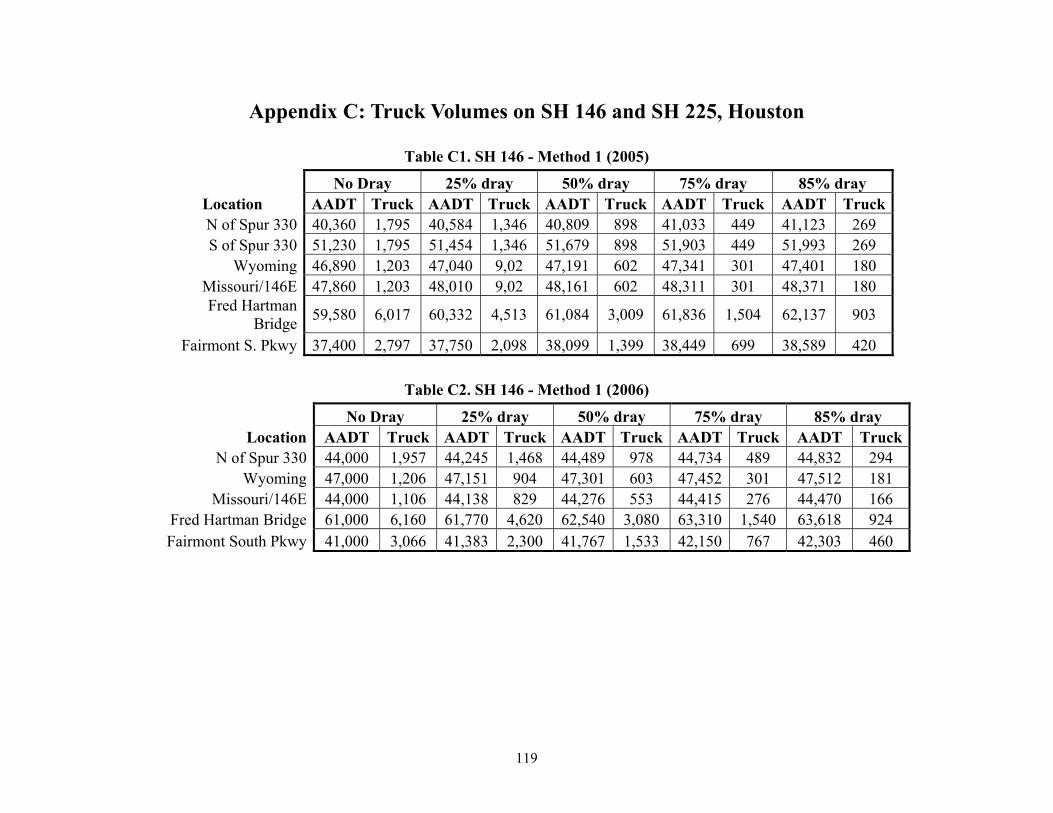
119

Appendix C: Truck Volumes on SH 146 and SH 225, Houston

Table C1. SH 146 - Method 1 (2005)

No Dray 25% dray 50% dray 75% dray 85% dray Location AADT Truck AADT Truck AADT Truck AADT Truck AADT TruckN of Spur 330 40,360 1,795 40,584 1,346 40,809 898 41,033 449 41,123 269 S of Spur 330 51,230 1,795 51,454 1,346 51,679 898 51,903 449 51,993 269

Wyoming 46,890 1,203 47,040 9,02 47,191 602 47,341 301 47,401 180 Missouri/146E 47,860 1,203 48,010 9,02 48,161 602 48,311 301 48,371 180 Fred Hartman

Bridge 59,580 6,017 60,332 4,513 61,084 3,009 61,836 1,504 62,137 903

Fairmont S. Pkwy 37,400 2,797 37,750 2,098 38,099 1,399 38,449 699 38,589 420


No Dray 25% dray 50% dray 75% dray 85% dray Location AADT Truck AADT Truck AADT Truck AADT Truck AADT Truck

N of Spur 330 44,000 1,957 44,245 1,468 44,489 978 44,734 489 44,832 294 Wyoming 47,000 1,206 47,151 904 47,301 603 47,452 301 47,512 181

Missouri/146E 44,000 1,106 44,138 829 44,276 553 44,415 276 44,470 166 Fred Hartman Bridge 61,000 6,160 61,770 4,620 62,540 3,080 63,310 1,540 63,618 924 Fairmont South Pkwy 41,000 3,066 41,383 2,300 41,767 1,533 42,150 767 42,303 460

120



N of Spur 330 40,360 1,795 39,911 1,346 39,463 898 39,014 449 38,834 269 S of Spur 330 51,230 1,795 50,781 1,346 50,333 898 49,884 449 49,704 269

Wyoming 46,890 1,203 46,589 902 46,289 602 45,988 301 45,867 180 Missouri/146E 47,860 1,203 47,559 902 47,259 602 46,958 301 46,837 180

Fred Hartman Bridge 59,580 6,017 58,076 4,513 56,572 3,009 55,067 1,504 54,466 903 Fairmont South Pkwy 37,400 2,797 36,701 2,098 36,002 1,399 35,302 699 35,023 420



N of Spur 330 44,000 1,957 43,511 1,468 43,022 978 42,532 489 42,337 294 Wyoming 47,000 1,206 46,699 904 46,397 603 46,096 301 45,975 181

Missouri/146E 44,000 1,106 43,724 829 43,447 553 43,171 276 43,060 166 Fred Hartman Bridge South 61,000 6,160 59,460 4,620 57,920 3,080 56,380 1,540 55,764 924

Fairmont South Pkwy 41,000 3,066 40,233 2,300 39,467 1,533 38,700 767 38,394 460

Table C5. SH 225 - Method 1 (2005) No Dray 25% dray 50% dray 75% dray 85% dray

Location AADT Truck AADT Truck AADT Truck AADT Truck AADT TruckN of Spur 330 76,150 6,442 76,955 4,832 77,761 3,221 78,566 1,611 78,888 966 S of Spur 330 93,390 7,771 94,361 5,828 95,333 3,886 96,304 1,943 96,693 1,166

Wyoming 122,340 9,704 123,553 7,278 124,766 4,852 125,979 2,426 126,464 1,456

121



N of Spur 330 80,000 6768 80,628 3,767 80,828 1,657 80,615 410 80,416 147 Wyoming 98,000 8155 98,757 4,540 98,999 1,997 98,741 494 98,502 177

Missouri/146E 114,000 9042 114,839 5,036 115,108 2,217 114,823 549 114,558 197



N of Spur 330 76,150 6,442 75,532 1,854 74,914 1,236 74,296 618 74,049 371 S of Spur 330 93,390 7,771 93,110 839 92,831 560 92,551 280 92,439 168

Wyoming 122,340 9,704 122,060 839 121,781 560 121,501 280 121,389 168



N of Spur 330 80,000 6,768 78,308 5,076 76,616 3,384 74,924 1,692 74,247 1,015 Wyoming 98,000 8,155 95,961 6,116 93,923 4,077 91,884 2,039 91,069 1,223

Missouri/146E 114,000 9,042 111,739 6,782 109,479 4,521 107,218 2,261 106,314 1,356

123

Appendix D: Houston Dray GPS Data Analysis

In the first year of the study the researchers interviewed dray drivers as to their use of the road network. Commonly asked questions included which roads are most important in making their deliveries, where they encountered the worst congestion, how many miles they placed on the road network, and how frequently they left the Houston area. From these interviews both with drivers and with fleet operators, the researchers developed a general sense of the average daily activity of the dray driver. However, the researchers sought to gain more precise information that would be quantitative rather than anecdotal in nature to ensure that the information received through oral interviews was correct. This was particularly important when querying drivers on metrics for which they might not have a precise mental picture, such as the average time that they spent waiting outside of the container terminal gates. It is natural when recalling such events to draw attention to exceptional incidents, such as an occurrence of abnormally long delay, rather than describing the most common experience, which often goes virtually unnoticed. Fortunately the technology of fleet management has been advancing rapidly in recent years. Devices that are used to provide information on truck usage and driver activity are becoming far more widespread within the trucking industry as their capital cost requirements are reduced and the advantages that can be gained through savings in driver hours and fuel, two increasingly precious resources, are recognized. The researchers studied the technical specifications of some of the devices that were currently on the market and in use by dray fleet operations similar to Houston’s. In order to provide for effective feedback, the device had to be able to capture the speed of the vehicles, the number of stops, the amount of waiting time compared to drive time, and to visually depict the route on a digital map. It was also important that the device calculate the cumulative distance that the vehicle traveled in the course of a day, as this was the clearest metric of the vehicle’s use of the road network. The device chosen was initially recommended by a dray firm operating in Houston that was experimenting with fleet-management software.

Typically the fleet-management devices are engineered so that the drivers cannot manipulate them. They are, therefore, placed under the dashboard and connected directly to the power source of the engine and run at all times. For the purpose of this study, however, the researchers required a mobile device that could be moved from truck to truck so as to take a broader sample of activities that would not bias the operation of a single operator. The software that was selected is produced by a firm called @Road, a subsidiary of Trimble. The hardware used for the experiment is a GPS-enabled cell phone that has no special modifications. With this combination of hardware and software, the researchers approached dray firms about allowing these devices to be placed into their trucks for a predefined period of time period of at least one week. Because the dray industry is dominated by owner-operators, the researchers needed the authorization of each individual driver to place the device in their own truck. Before each experiment, the researchers spoke briefly with the drivers to ensure that they perform what could be termed general dray operations, i.e., deliveries to multiple customers based on random dispatch orders. If drivers worked on an exclusive contract in which they made deliveries to a certain distribution center again and again, their value to this sample might be reduced. Truck samples were taken over a period of two months between February 4 and March 30. In almost all cases the GPS devices recorded the entire day’s activity. Figure D.1 shows the vehicle miles traveled (VMT) totals for each day from the activity log in no particular order.

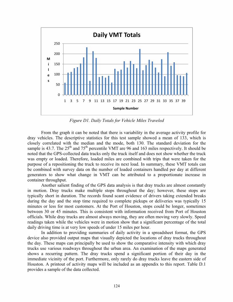
124

Figure D1. Daily Totals for Vehicle Miles Traveled

From the graph it can be noted that there is variability in the average activity profile for dray vehicles. The descriptive statistics for this test sample showed a mean of 133, which is closely correlated with the median and the mode, both 130. The standard deviation for the sample is 43.7. The 25th and 75th percentile VMT are 96 and 163 miles respectively. It should be noted that the GPS-collected data tracks only the truck itself and does not show whether the truck was empty or loaded. Therefore, loaded miles are combined with trips that were taken for the purpose of a repositioning the truck to receive its next load. In summary, these VMT totals can be combined with survey data on the number of loaded containers handled per day at different generators to show what change in VMT can be attributed to a proportionate increase in container throughput.

Another salient finding of the GPS data analysis is that dray trucks are almost constantly in motion. Dray trucks make multiple stops throughout the day; however, these stops are typically short in duration. The records found scant evidence of drivers taking extended breaks during the day and the stop time required to complete pickups or deliveries was typically 15 minutes or less for most customers. At the Port of Houston, stops could be longer, sometimes between 30 or 45 minutes. This is consistent with information received from Port of Houston officials. While dray trucks are almost always moving, they are often moving very slowly. Speed readings taken while the vehicles were in motion show that a significant percentage of the total daily driving time is at very low speeds of under 15 miles per hour.

In addition to providing summaries of daily activity in a spreadsheet format, the GPS device also provided output maps that visually depicted the locations of dray trucks throughout the day. These maps can principally be used to show the comparative intensity with which dray trucks use various roadways throughout the urban area. An examination of the maps generated shows a recurring pattern. The dray trucks spend a significant portion of their day in the immediate vicinity of the port. Furthermore, only rarely do dray trucks leave the eastern side of Houston. A printout of activity maps will be included as an appendix to this report. Table D.1 provides a sample of the data collected.

0

50

100

150

200

250

1 3 5 7 9 11 13 15 17 19 21 23 25 27 29 31 33 35 37 39

Miles

Sample Number

Daily VMT Totals

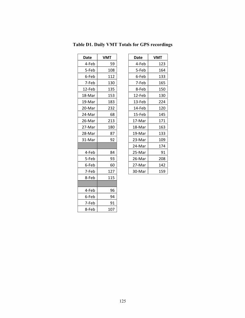
125

Table D1. Daily VMT Totals for GPS recordings

Date VMT Date VMT

4-Feb 59 4-Feb 1235-Feb 108 5-Feb 164

6-Feb 112 6-Feb 1337-Feb 130 7-Feb 165

12-Feb 135 8-Feb 15018-Mar 153 12-Feb 130

19-Mar 183 13-Feb 22420-Mar 232 14-Feb 120

24-Mar 68 15-Feb 14526-Mar 213 17-Mar 171

27-Mar 180 18-Mar 16328-Mar 87 19-Mar 133

31-Mar 92 23-Mar 109 24-Mar 174

4-Feb 84 25-Mar 915-Feb 93 26-Mar 208

6-Feb 60 27-Mar 1427-Feb 127 30-Mar 159

8-Feb 115

4-Feb 96 6-Feb 94 7-Feb 91 8-Feb 107

the impacts of port, rail, and border drayage activity...

Documents