The Impacts of Natural Gas Prices on the California Economy: Final Report

PREPARED FOR:

The California Natural Gas Advisory Group

PREPARED BY:

Global Insight, Inc. Global Energy Services, United States

24 Hartwell Avenue, Lexington MA 02421-3158 Phone: +1 (781) 301-9100

Fax: +1 (781) 3010-9407

U.S. Regional Services, United States 800 Baldwin Tower, Eddystone PA 19022

Phone: +1 (610) 490-2500 Fax: +1 (610) 490-2770

www.globalinsight.com

February 2006

TABLE OF CONTENTS

EXECUTIVE SUMMARY ................................................................................................ 1

INTRODUCTION........................................................................................................... 12

Study Objectives .....................................................................................................................................12

Requirements of the Study Sponsors .....................................................................................................12

BACKGROUND............................................................................................................ 14

Natural Gas Supply and Demand in California .......................................................................................14

Recent Price Trends ...............................................................................................................................17

STUDY ASSUMPTIONS............................................................................................... 19

Natural Gas Price Scenarios...................................................................................................................19

Crude Oil and Natural Gas Prices...........................................................................................................21

Economic Sectors Dependent on Natural Gas .......................................................................................22

STUDY METHODOLOGY............................................................................................. 27

Preparing Energy Forecasts ...................................................................................................................27

Estimating U.S. Macroeconomic Impacts ...............................................................................................28

Estimating California Economic Impacts.................................................................................................28

Revisions to the Global Insight California Forecast Model .....................................................................28

ECONOMIC IMPACTS ................................................................................................. 31

Economic Effects of Changes in Natural Gas Prices..............................................................................31

Impacts on the U.S Economy..................................................................................................................31

Impacts on the California Economy ........................................................................................................32

Impacts on Major End Users...................................................................................................................38

Impacts in Northern and Southern California..........................................................................................43

Results of Other Studies .........................................................................................................................45

SUMMARY.................................................................................................................... 47

APPENDIX A: DETAILED ECONOMIC IMPACTS IN CALIFORNIA........................... 51

APPENDIX B: INTERVIEWS WITH ENERGY-INTENSIVE INDUSTRIES ................... 54

APPENDIX C: ECONOMIC IMPACTS IN CALIFORNIA BY SECTOR........................ 65

1

EXECUTIVE SUMMARY

Objective The objective of this study is to assess the impacts on the California economy of changes in natural gas prices. Since California is more dependent on natural gas as a source of energy than are most other states, a continuing concern is the negative economic effect that a long-term, sustained rise in the price of natural gas could have on its economy. A second objective of this study is to calculate the positive economic benefits that would occur if future natural gas prices were lower than had been expected previously due to the adoption of policies favorably affecting supply and demand conditions and infrastructure investments.

Study Background and Assumptions Natural gas prices in California and the United States have been steadily rising in recent years. In 1999, the average annual wholesale natural gas price at the Southern California border at Topock was $2.32/million British Thermal Units ($/MMBtu), slightly greater than the Henry Hub or U.S. reference price of $2.27/MMBtu. The annual Topock Border price rose during the electricity crisis of 2001 and declined in 2002 but has been rising steadily since, with Global Insight forecasting an annual Topock border price in 2005 of $6.79/MMBtu in August 2005 (i.e., before the Gulf hurricanes Katrina and Rita). Yet due to the shut-ins of natural gas production—a result of the hurricanes—and continued high demand for gas for electric power generation, natural gas prices in California have risen throughout 2005 but remain lower than those in other parts of the United States. According to the Energy Information Administration (EIA), the California composite wholesale natural gas spot price (an average of the Malin, PG&E citygate, and Topock prices) on November 15, 2005 was $7.80/MMBtu, up 24% and $1.90/MMBtu from year-ago prices, and 71% greater than the price of two years ago ($4.56/MMBtu). The Topock price had risen to $7.75/MMBtu by November 15 as compared with the Henry Hub price of $9.21/MMBtu that same day.

These price increases have cost California consumers and industries millions of dollars of increased costs to heat their homes, generate electricity and to provide energy for manufacturing processes. Final users of natural gas in California spent about $19.1 billion (nominal $) to buy natural gas in 2005, including $5.8 billion by households and $4.8 billion by utilities to generate electricity. Therefore, even a 5% reduction in natural gas prices would generate about $1 billion in short-term savings to consumers and industries.

California is part of the North American natural gas market through its connections to the intercontinental pipeline network. Since demand, supply, and infrastructure factors in North America determine natural gas prices, California often has little direct control over market prices. Because natural gas received from U.S. Southwest production basins (i.e., San Juan and Permian Basins) constitutes the marginal supply of natural gas in California, the Southern California border price at the Topock hub is a major indicator of natural gas prices in California.

The study period is the 2006–16 timeframe. Global Insight and the Natural Gas Study Advisory Committee—which is comprised of the California Energy Commission, Pacific Gas & Electric Company, Southern California Edison Company, Southern California Gas Company and San Diego Gas & Electric Company—defined three wholesale natural gas price scenarios in California using the delivered price of natural gas at Topock (i.e., called the Topock border price

2

in the remainder of the study) as the reference price of gas. The Advisory Committee and Global Insight also agreed that the three price scenarios should vary based on the differences in the Topock border and Henry Hub prices, enabling the study to consider the economic impact when California and U.S. wholesale natural gas prices were the same, when the California price was greater, and when the California price was less. The differences between the Topock border and Henry Hub prices were defined as the basis differences for each price scenario. The Advisory Committee decided to use the same oil price for all three scenarios (approximately $60/barrel by 2016) in nominal dollars for the WTI/NYMEX contract specification so that the economic impacts would be attributable only to the differences in the natural gas prices.

The following gas price scenarios and the basis differences were used in estimating the economic impacts of alternative natural gas wholesale price levels on the California economy. The gas price scenarios are not forecasts of natural gas prices, but are intended as study parameters in order to assess the economic impacts of natural gas prices on the California economy.

• Low-price scenario: The average annual Topock border price will reach $5.00/MMBtu (in constant 2005 dollars) by 2016. The Henry Hub price will be $0.75/MMBtu higher than the Topock border price in 2007, a basis difference that will remain constant through 2016.

• Middle-price scenario: The average annual Topock border price will reach $7.50/MMBtu (in constant 2005 dollars) by 2016. No basis difference exists between the Topock border and Henry Hub prices in the Middle-price scenario.

• High-price scenario: The average annual Topock border price will reach $10.00/MMBtu (in constant 2005 dollars) by 2016. The Henry Hub price will be $0.25/MMBtu less than the Topock price by 2007 and then decline to $0.75/MMBtu lower than the Topock border price by 2009, a basis difference that will remain constant through 2016.

The three price scenarios were selected to define the probable maximum range of future gas prices in California on an annual average basis. Global Insight and the Advisory Committee believed that future wholesale natural gas prices would most likely neither exceed the levels in the High-price scenario, nor fail to meet the levels defined in the Low-price scenario. The Middle-price scenario was not defined as a baseline or most likely forecast.

Supply and Demand The California Energy Commission (CEC) forecast in November 2005 that total demand for natural gas in California will grow at an annual rate of 0.55% in the next decade. It will grow at faster annual rates of 1.76% in the Commercial sector and 1.33% in the Residential sector. By comparison, annual growth in demand by the power generation will approach but not meet the total statewide rate at 0.54%, while industrial demand will decline 0.77% annually. The supply and demand balance for natural gas in California depends on two factors: 1) sectors with the highest growth rates that drive demand and 2) the provision of new supplies. Demand growth will depend heavily on the use of natural gas in power generation, as 49% of the electricity generated in California in 2001 was produced by burning natural gas, and 41% of the electricity consumed in the state was generated by burning natural gas. The provision of new, lower-cost supply sources will depend in part upon policy options implemented in California. Adding pipeline capacity may not be enough to guarantee adequate supply, as several of the North

3

American basins upon which California depends for much of its natural gas face long-term production declines.

Methodology Global Insight used three proprietary econometric models to estimate the economic impacts presented in this study. Three forecasting steps were required: 1) prepare three alternative U.S. energy forecasts with our Energy model using the Henry Hub and oil prices described above as inputs, 2) prepare three alternative U.S. macroeconomic forecasts using the three energy forecasts as inputs, and 3) prepare three forecasts for California using our enhanced econometric model for the State. Key outputs from the U.S. energy and macroeconomic forecasts were wholesale and retail energy prices for major types of energy, especially natural gas, along with changes in such indicators as gross domestic product (GDP), employment, industrial production, inflation, and personal income. The impacts in California were derived using Global Insight’s enhanced econometric model for the state, which was revised to directly consider the U.S. and California natural gas price levels in each of the three price scenarios. We combined time series data on regional and U.S. energy prices and the energy use shares (in British thermal units or Btus) by sector to derive a weighted price of energy by sector in California. We then econometrically estimated the historic relationship between the economic growth of a sector and its weighted average price of energy in order to capture the way in which changing energy prices had historically affected levels of employment and output in the sector. Global Insight also conducted a number of interviews with representatives of companies operating in California that are major users of natural gas in order to determine how they have responded to changes in natural gas prices in the past and how they would likely do so in the future.

Economic Effects of Changes in Natural Gas Prices Higher natural gas prices can affect a state economy negatively in three ways: 1) direct effects—the amount end users must spend for natural gas rises; 2) indirect effects—end users buy fewer inputs from suppliers because their sales decline due to price increases caused by higher natural gas prices; and 3) induced effects—employment declines at the directly and indirectly affected firms lead to drops in local expenditures of disposable income. In the short run, a business has two options to offset the higher natural gas costs: pass along some or all of them to its customers; and reduce other non-gas costs by lowering employment or buying less from suppliers. In the short run, households are also forced to spend more for natural gas and less for other goods and services. Supplying firms then experience reduced sales, leading them to also reduce purchases from their suppliers, and so forth. If a manufacturing firm that spends more to buy natural gas lays off workers or reduces wages, spending at local retail stores will decline, causing them to reduce employment as sales fall, and so on.

Economic Impacts in California Direct Impacts

In our study, the direct economic effect is defined as the amount of money spent by final users to purchase natural gas under each of the three scenarios. In the High-price scenario, the amount of money spent will be higher than that spent in the Middle-price and Low-price scenarios or than that experienced as a cost increase by households and businesses as

4

compared with expenditures in the other two scenarios. By contrast, the amount of money spent to purchase natural gas in the Low-price scenario will be substantially lower than that spent in the other two scenarios, resulting in a cost savings to households and businesses. We estimated the following expenditures for natural gas under the three scenarios in 2010–16.

• Low-price scenario: Natural gas purchases of $18.8 billion (nominal $) in 2010 and $20.3 billion (nominal $) in 2016.

• Middle-price scenario: Natural gas purchases of $22.4 billion (nominal $) in 2010, $3.6 billion more than in the Low-price scenario; and $26.9 billion (nominal $) in 2016, $6.7 billion higher than in the Low-price scenario.

• High-price scenario: Natural gas purchases of $26 billion (nominal $) in 2010, $7.2 billion above the Low-price scenario; and $33.2 billion (nominal $) in 2016, $13 billion higher than in the Low-price scenario.

These direct effects will spread through the California economy via the indirect and induced effects described above. The Global Insight forecast models produce estimates of the total net change in economic activity, so the direct, indirect, and induced effects are included in the results presented herein. It is important to note that the economic impacts presented in this study are cumulative and will occur with time as firms and households make continuous adjustments to natural gas price levels. The economic impacts in 2016 will be the result of adjustments made in the 2006–15 timeframe by the affected firms and households. Because our models use time series data, they are able to capture these adjustments over time. The economic impacts produced by our models include direct, indirect, and induced effects.

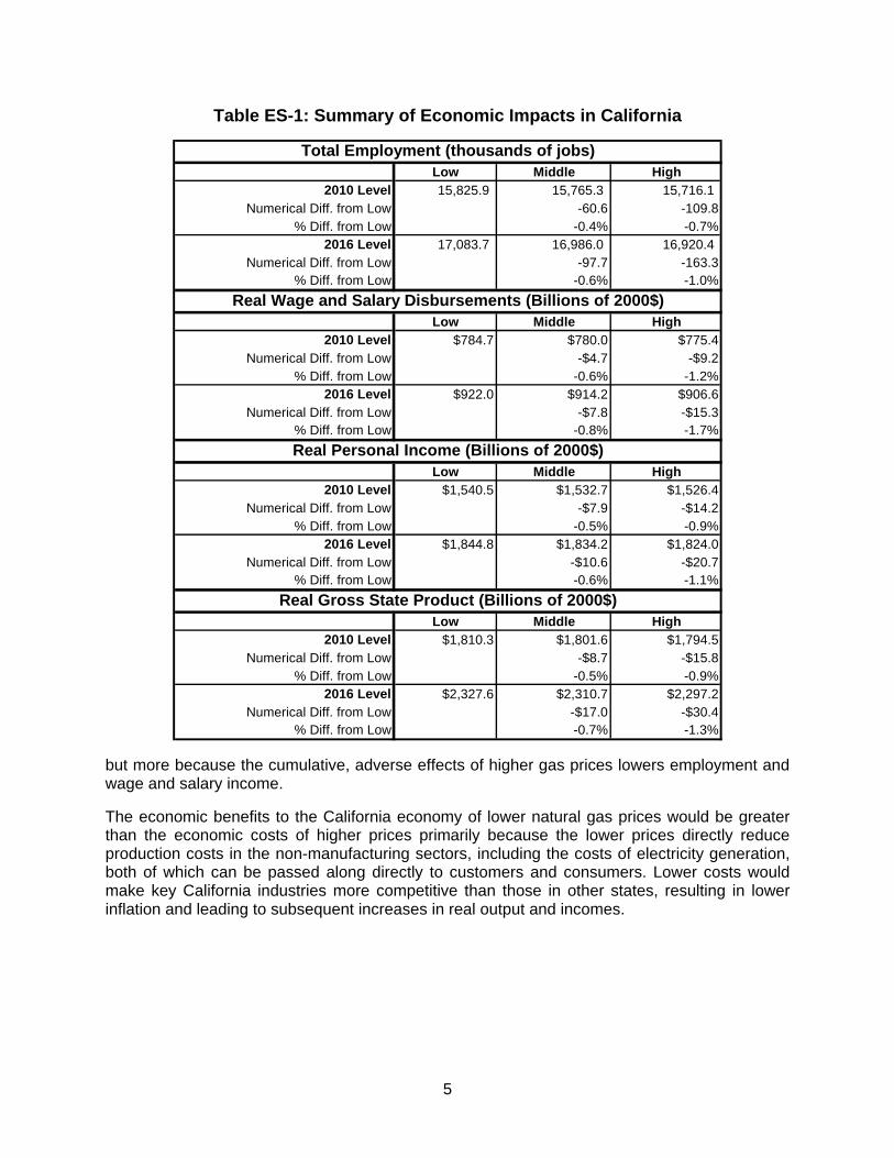
Impact Summary The economic impacts in California for the three price scenarios are presented in Table ES-1, followed by impacts for the major end-user groups. The table shows that by 2016 employment in the Middle-price and High-price scenarios would total 97,700 and 163,300 fewer jobs than in the Low-price scenario. Similarly, real gross state product (GSP, in constant year 2000 dollars) in 2016 under the High-price scenario will be $30.4 billion less than that in the Low-price scenario. Global Insight finds that the best measure of the economic impacts of the three scenarios is real GSP (sometimes referred to as real value-added output) in constant year 2000 dollars as this measure is defined on the same basis as GDP and is expressed in the same base year. The differences, in numerical and percentage terms, between the levels of economic activity in the Low-, Middle- and High- scenarios from the Low-price scenario, in both numerical and percentage terms, increase during 2010–16 timeframe, showing that the impacts are cumulative.

These widening differences are the result of adjustments made by the affected households and companies during the study period to adapt to rising natural gas prices, such as investments in more energy-efficient equipment and fuel switching capability, changes in production processes, reduced labor costs from eliminated shifts and layoffs, plant closings, and operations being shifted out of state.

The adverse impacts of the Middle- and High-price scenarios by 2016 are higher for both real GSP and real personal income in part because sizable labor cost savings have already been realized in the natural gas-intensive sectors in California during the past few years; therefore, firms must find alternative ways to cope with rising natural prices other than cutting jobs. The impacts of the Middle- and High-price scenarios on real wage disbursements are larger in percentage terms than are the impacts on personal income in part because the higher gas prices will increase the rate of inflation,

5

Table ES-1: Summary of Economic Impacts in California

Low Middle High2010 Level 15,825.9 15,765.3 15,716.1

Numerical Diff. from Low -60.6 -109.8% Diff. from Low -0.4% -0.7%

2016 Level 17,083.7 16,986.0 16,920.4 Numerical Diff. from Low -97.7 -163.3

% Diff. from Low -0.6% -1.0%

Low Middle High2010 Level $784.7 $780.0 $775.4

Numerical Diff. from Low -$4.7 -$9.2% Diff. from Low -0.6% -1.2%

2016 Level $922.0 $914.2 $906.6Numerical Diff. from Low -$7.8 -$15.3

% Diff. from Low -0.8% -1.7%

Low Middle High2010 Level $1,540.5 $1,532.7 $1,526.4

Numerical Diff. from Low -$7.9 -$14.2% Diff. from Low -0.5% -0.9%

2016 Level $1,844.8 $1,834.2 $1,824.0Numerical Diff. from Low -$10.6 -$20.7

% Diff. from Low -0.6% -1.1%

Low Middle High2010 Level $1,810.3 $1,801.6 $1,794.5

Numerical Diff. from Low -$8.7 -$15.8% Diff. from Low -0.5% -0.9%

2016 Level $2,327.6 $2,310.7 $2,297.2Numerical Diff. from Low -$17.0 -$30.4

% Diff. from Low -0.7% -1.3%

Total Employment (thousands of jobs)

Real Gross State Product (Billions of 2000$)

Real Personal Income (Billions of 2000$)

Real Wage and Salary Disbursements (Billions of 2000$)

but more because the cumulative, adverse effects of higher gas prices lowers employment and wage and salary income.

The economic benefits to the California economy of lower natural gas prices would be greater than the economic costs of higher prices primarily because the lower prices directly reduce production costs in the non-manufacturing sectors, including the costs of electricity generation, both of which can be passed along directly to customers and consumers. Lower costs would make key California industries more competitive than those in other states, resulting in lower inflation and leading to subsequent increases in real output and incomes.

6

Impacts by End User Households

Households will be affected directly by rising natural gas prices under the High-price scenario as they spend more to purchase natural gas used for heating and cooking, and indirectly via higher electricity prices. Table ES-2 presents the changes in spending per household for natural gas and electricity under the three scenarios in nominal dollars, as households make expenditure decisions based on nominal values.

Table ES-2: Changes in Household Spending for Natural Gas and Electricity

Low M iddle H igh2010 Level $440 $510 $578

Num erica l D iff. from Low $70 $138% D iff. from Low 15.9% 31.4%

2016 Level $440 $558 $673Num erica l D iff. from Low $118 $233

% D iff. from Low 26.8% 53.0%

Low M iddle H igh2010 Level $937 $970 $1,002

Num erica l D iff. from Low $33 $65% D iff. from Low 3.5% 6.9%

2016 Level $1,097 $1,152 $1,203Num erica l D iff. from Low $55 $106

% D iff. from Low 5.0% 9.7%

Low M iddle H igh2010 Level $144,024 $143,623 $143,436

Num erica l D iff. from Low -$401 -$588% D iff. from Low -0 .3% -0.4%

2016 Level $187,677 $187,208 $185,954Num erica l D iff. from Low -$469 -$1,723

% D iff. from Low -0 .2% -0.9%

Natural G as Spending per Household (Nom inal $)

E lectricity Spending per Household (Nom inal $)

Average Household Personal Incom e (Nom inal $)

In the High-price scenario, annual spending per household for natural gas would be $233 higher than it would in the Low-price scenario by 2016, due primarily to the higher Topock border price, which in turn will increase natural gas retail prices. Annual per household spending for electricity would be $106 higher, for a combined increase of $339. Consumer Expenditure Survey data for 2003 showed that about 2.2% of annual consumer expenditures (or 1.3% of average household personal income) by California households were allotted for natural gas and electricity. A major concern is the effect of the High-price scenario on low-income households (those with annual consumption expenditures of less than $25,000); in 2003 they spent more than 3.0% on natural gas and electricity and thus would be more affected by the declines in disposable household personal income.

Under the Middle- and High-price scenarios per-household real disposable income will be $523 and $1,088 less than the Low-price level of $110,076 by 2016. These real income decreases are produced by the cumulative, overall declines in economic activity that will have occurred by

7

2016 as shown in Table ES-1 and when combined with inflationary effects of higher natural gas and electricity prices. The combination of the decreases in real household disposable income in the Middle-price and High-price scenarios and higher spending for natural gas and electricity will adversely affect California households as they must alter their spending patterns by using more of their incomes to purchase natural gas and electricity, leaving less available to buy other goods and services.

Manufacturing Sector

By 2016, manufacturing employment in the Middle- and High-price scenarios would account for 15,200 and 32,500 fewer jobs than in the Low-price scenario. Employment has been declining steadily in the California manufacturing sector for years; about 321,000 jobs were eliminated in 2000–05. We forecast that manufacturing employment will continue to decline, but at a slower rate because of the large number of jobs that have already been eliminated; by 2016, manufacturing employment would total about 22,000 fewer jobs than it does at present, falling from its current 10.4% share of total employment to 9.0%. The Middle- and High-price scenarios will accelerate a trend that is already underway, with the latter more than doubling the forecast job loss. The percentage impacts in real manufacturing GSP would be higher than those for employment; under the High-price scenario it would be 3.3% lower than in Low-price scenario by 2016.

The lower impacts on employment than on real GSP indicate, as confirmed during interviews, that the natural-gas intensive sectors in the state have been responding to higher natural gas prices by lowering production costs and eliminating jobs. In the future, with most of the job cuts already taken, responses to sustained higher natural gas prices would have to come primarily through efforts to reduce the costs of production or increase productivity and energy use efficiency. Our results suggest that the price effects will predominate in the manufacturing sector, especially as energy expenditures fall, since the cost savings can be immediately captured and passed along in the form of lower prices or higher profits, or invested in other more productive ways.

Private, Services-Providing Sectors

The impacts on the private, services-providing (PSP) sectors in both absolute and percentage terms will be similar to the overall impacts on the total economy presented in Table ES-1, especially for the High-price scenario. The PSP sectors currently account for about 70% of total real GSP in California, so on an aggregate basis, most of the impacts of higher natural gas prices will occur in these sectors. The primary economic effects of these prices will increase the costs of occupying office space, including electricity. We estimate that in 2016, real GSP in the PSP sectors in the High-price scenario will be $16.3 billion less than in the Low-price scenario, or about 54% of the total difference in real GSP. This lower impact share is unsurprising, as PSP businesses will be less affected by higher natural gas prices than manufacturing companies will be.

Government Sector

The economic impacts of gas prices on the government sector will be relatively small, again because the primary effect will be seen in the costs of occupying office space and using electricity. Some exceptions exist, however; notably, government agencies engaged in the generation, purchase, and sale of electric power, and Metropolitan Transportation agencies that purchase large amounts of electric power to operate subways. Government agencies most susceptible to changes in natural gas wholesale prices include those that enter into long-term

8

contracts to purchase either large amounts of natural gas for generating electricity or large amounts of wholesale electric power, with the electric power later sold at retail. We forecast that real GSP in the government sector (Federal, State, and Local) in 2016 under the High-price Scenario will be about $0.8 billion less than in the Low-price Scenario.

Electricity Generation

One of the primary direct effects of alternative natural gas prices will be on the cost of generating electricity because California generates a much higher share of its electricity using natural gas than does the rest of the country. According to the EIA, in 2001, slightly more than 49% of electric power generated in California was produced by burning natural gas; only 1.0% was made by burning coal, as compared with U.S. shares of 16.4% and 51.2%, respectively. Higher natural gas prices will directly raise the price of generating electricity, requiring businesses and households to pay more to obtain it and providing them an incentive to use less of it. We estimate that by 2016, the cost of natural gas purchased by California electric utilities and used in generating electric power in the Middle- and High-price scenarios will be $6.5 billion and $8.3 billion greater than in the Low-price Scenario, producing higher retail electricity prices and leading to the aforementioned negative impact on households.

Impacts in Northern and Southern California Global Insight estimated the impacts of high natural gas prices on Northern and Southern California regions; the latter was comprised of nine counties (Imperial, Los Angeles, San Luis Obispo, Santa Barbara, Orange, San Diego, Ventura, Riverside, and San Bernardino) and portions of four others (Kern, Tulare, Kings, and Fresno) based on utility service areas. The Northern California region covered the remainder of the state and generally aligns with the natural gas service area of the Pacific Gas and Electric Company (PG&E). Economic impacts for most indicators, such as real GSP and employment, will be slightly larger in Southern California than in Northern California because the former has higher concentrations of nine manufacturing sectors that are heavy users of natural gas. As a result, the Southern California economy is more sensitive to natural gas prices because of its economic structure; it would benefit more from lower natural gas prices and would be affected more adversely by higher prices.

Findings Level of State-wide Economic Activity Falls with Higher Prices

Natural gas prices under the Middle- and High-price scenarios would result in lower levels of economic activity in California by 2016 when compared with the levels in the Low-price scenario. Using outputs from our Energy and U.S. Macroeconomic models, the simulations performed with our enhanced California econometric model showed that sizable declines in the level of economic activity would be observed by 2016 in the High-price scenario, notably a $30.4 billion drop in real GSP ($42.2 billion in nominal terms) and the accompanying loss of 163,300 jobs. In percentage terms, the differences in levels of economic activity (as measured by total employment, total real GSP, and total real personal income) between the Low- and High-price Scenarios would range between 1.0 and 1.3% due to the large size of the California economy (currently 13.3% of US GDP). The percentage impacts would be higher in the manufacturing sector, where we forecast that by 2016, employment and real GSP would be 2.1% and 3.3% lower, respectively, in the High-price scenario than in the Low-price scenario.

9

Households Affected by Higher Energy Expenditures and Lower Incomes

California households would be adversely affected by sustained higher natural gas prices in several ways: 1) by the declines in the levels of economic activity, especially the loss of employment and the corresponding drop in wage and salary income; 2) by higher spending for natural gas and electricity, which reduces money available to purchase other goods and services; and 3) by higher inflation resulting from the increased nominal prices for energy, which in turn lowers real disposable personal income. We estimate that combined expenditures for natural gas and electricity would total $1,876 per household in nominal terms in the High-price scenario by 2016: $1,203 for electricity and $673 for natural gas. Increased spending by households on natural gas and electricity means they would have to limit their purchases of other goods and services. The percentage decline in the real wage and salary earnings in the High-price scenario as compared with that in Low-price scenario would be 1.7% by 2016, or far greater than the percentage drop in total real personal income, due to the combined effects of lower employment and higher price levels.

Marginal Impacts Decline as Natural Gas Prices Rise

Marginal economic impacts would decline as natural gas prices rise and increase as gas prices fall. The marginal economic impact is the change in the level of economic activity (e.g., employment, income, GSP) produced by a direct economic effect, such as an increase or decrease in the price of natural gas. The existing price level when a direct effect occurs largely determines the size of the marginal economic impact: if the natural gas price level is already high a further price rise of 1% would have a smaller, negative, marginal economic impact than a 1% increase from a low price level. Put in the context of this study, the number of jobs lost for each 1% increase in price between the Middle and High-price scenarios would be less than the number lost for each 1% increase in price between the Low- and Middle-price scenarios. The reverse would also occur: the increase in employment for each 1% decrease in price between the High- and Middle-price scenarios would be less than the increase in employment for each 1% decrease between the Middle- and Low-price scenarios. The declining marginal economic effects of rising natural gas prices were identified by estimating implicit employment elasticities (defined as the percent decline in employment for each 1% increase in natural gas prices between two scenarios).

Amid rising prices, the decline in marginal impacts means that up to a certain price level, most of the adjustments that can be made to reduce energy costs will have been implemented and the savings realized; beyond this price, little more can be done to lower energy use without also lowering production levels (i.e., no more workers can be laid off, energy use cannot be reduced any further, and all energy-efficient equipment has been installed). The energy cost savings that can be realized will become smaller, and the marginal costs required to obtain it will become increasingly higher. With falling prices, such as from the High- to the Low-price scenario, the reduction in natural gas and electricity expenditures are immediately realized, enabling businesses to either lower prices, increase profits, or invest the freed-up funds in more productive ways. At the same time, households have more money to spend on other goods and services.

Impacts of Higher Natural Gas Prices Increase in Time

Our study showed that the adverse economic impacts of the High- and Middle-price scenarios will increase with time in both absolute (e.g., using constant year 2000 dollars for GSP and income) and percentage terms when compared with those of the Low-price scenario. The primary reason is that the price levels for the three scenarios, in real terms, widen over time.

10

Businesses and households directly affected by sustained higher prices will continually adjust to sustained higher natural gas prices in order to reduce the amount they spend for natural gas and electricity, so that in time the differences in the levels of economic activity among the three scenarios will widen. This process of continual adjustment also means that by 2016 the differences in the levels of economic among the three price scenarios will be the cumulative result of all the adjustments that were made in the preceding 10 years. The tables presented in Section 5.0 and in Appendix A consistently show larger absolute and percent impacts in 2016 than they show in 2010.

California is More Sensitive to High Natural Gas Prices than the U.S. Economy

Our study showed that the California economy is somewhat more sensitive to higher natural gas prices than is the U.S. economy. We corrected for differences in the levels of wholesale natural gas prices in the United States and in California under the three scenarios by estimating implicit elasticities for such key indicators such as real GDP/GSP, employment, and personal income. The elasticities consistently showed that a 1% increase in the wholesale price of natural gas in the United States would generally have a smaller, adverse impact in percentage terms than a 1% increase in wholesale natural gas prices in California. The California economy is more sensitive to natural gas prices for a couple of reasons: 1) its major natural gas using industries obtain higher shares of their energy inputs (on a Btu basis) from natural gas than do the same sectors at the U.S. level; and 2) almost half of the electric power generated in California comes from burning natural gas, resulting in higher retail electricity prices for the major end-user groups, such that the negative effects of the higher energy expenditures will spread throughout the economy. Higher residential electricity prices are significant because California households currently spend about $1.91 for electricity for every $1.00 spent for natural gas.

Structure of California’s Economy would be Unaffected

The composition or structure of a state economy is shown by the types of goods and services it produces, and is usually measured by the relative shares of economic activity, such as employment and output, by economic sector (i.e., what percent of state-wide employment and real GSP is in the manufacturing sector). A number of domestic, regional, and global economic forces have and will continue to change the structures of both the U.S. and California economies. Many of these factors are well-known, including:

• The continuing decline of the manufacturing sector in California and throughout the United States

• Increased global competition, such as the rises of China and India • Off-shoring • Current and future trade agreements, such as NAFTA • The competitive advantages and disadvantages of the California economy, such as high

labor and housing costs in its largest MSAs • Regional migration trends of households and businesses in the western United States • California business taxes and environmental and energy policies

Although these factors will continue to effect economic growth in California, we conclude that, when considered in the context of all these powerful factors, higher sustained natural gas prices would have a minor impact on the structure of the California economy. The structure of the state economy will continue to evolve due to the aforementioned factors; the primary structural effect of higher natural gas prices would be to accelerate the decline of the manufacturing sector, but this downward trend will continue independent of the future price of wholesale natural gas.

11

Conclusion

Our study shows that sustained, higher natural gas prices in the High- and Middle-price scenarios would have negative effects on California households and commercial and industrial end-users, resulting in cumulative reductions in the forecasted levels of employment, real GSP, and income by 2016. Higher natural gas prices would also accelerate the continuing loss of manufacturing jobs, produce higher utility bills for natural gas and electricity customers, and result in lower levels of household income. By contrast, lower natural gas prices in the Low-price scenario would benefit directly residential, industrial, and commercial customers alike, as they would spend less to purchase natural gas and electricity, resulting in higher levels of employment, GSP, and real incomes by 2016.

12

INTRODUCTION

Natural gas prices in California are currently rising, although they remain lower than those in most other parts of the United States. According to the Energy Information Administration (EIA), the California composite wholesale natural gas spot price (an average of the Malin, PG&E citygate, and Southern California border price at Topock) on November 15, 2005 was $7.80/million British Thermal Units ($/MMBtu), up 24% and $1.90/MMBtu from year-ago prices, and 71% greater than the price seen two years ago ($4.56/MMBtu). The Topock border price had climbed to as much as $11.67/MMBtu in late October 2005. By contrast, the Henry Hub natural gas price on November 15 was $9.21/MMBtu. The final users of natural gas in California will spend about $16.6 billion to buy natural gas in 2005, so even a 5% reduction in its price would generate a considerable short-term savings for companies, utilities, and households.

California is part of the North American natural gas market through its connections to the intercontinental pipeline network. Demand, supply, and infrastructure factors in North America determine natural gas prices, so California often has little direct control over market prices. For example, in February 2003, a time when California demand was moderate, California natural gas wholesale prices spiked due to extreme weather conditions in the Northeast. Such is not the situation today, however: the increasing national hunt for a limited supply of natural gas is driving prices higher, and therefore, California must focus on those actions that can help California consumers and that are within its control. Natural gas sent from southwest production areas constitutes its marginal supply, and thus the Topock Border price is an indicator of natural gas prices in California.

Study Objectives The objective of this study was to assess the impacts of changes in natural gas prices on the California economy. Because California is more dependent on natural gas as a source of energy than are most other states, the adverse economic effect that a continuing, long-term rise in the price of natural gas could have on the statewide economy is a major concern, especially if California natural gas prices begin to exceed U.S. prices. It was also important to estimate the economic benefits that could occur if future natural gas prices were lower than had been expected through favorable supply and demand conditions and infrastructure investments.

Requirements of the Study Sponsors The sponsors of the study (listed in the next section) had the following requirements that determined the scope of the work and the methodologies applied.

• Use publicly available economic and gas price data to conduct the study. • Make study methodology, data sources, and results available to the public. • Measure macroeconomic impacts of various gas price scenarios on income,

employment, key industrial users of gas, in Northern California, Southern California, and the state economy (GSP) as a whole.

Representatives of its sponsoring organizations were asked to serve on an advisory committee for the study; its purpose was to determine the scope of the study, review and approve study approaches, provide technical guidance and input since all its members were knowledgeable about the California natural gas sector, and review and provide comments on interim deliverables and the draft and final reports. Members of the Advisory Committee included:

13

• Les Buchner, Pacific Gas and Electric Company • Robert Cowden, Pacific Gas and Electric Company • Herb Emmrich, Southern California Gas Company and San Diego Gas & Electric

Company • Jairam Gopal, California Energy Commission • Karen Griffin, California Energy Commission • Richard Hendrix, Pacific Gas and Electric Company • Dave Maul, California Energy Commission • Luis Pando, Southern California Edison Company • Scott Wilder, Southern California Gas Company and San Diego Gas & Electric Company

14

BACKGROUND

Natural Gas Supply and Demand in California California is literally at the end of the natural gas pipeline, and as such has experienced periods of both oversupply and undersupply relative to its demand growth. Also, a growing shortfall of the natural gas commodity is itself creating repercussions in gas prices. The loss of production from the 2005 hurricane season will amount to more than 700 billion cubic feet (bcf), constraining potential users of natural gas and creating a very high price environment. Although such disruptions are hopefully unique and temporary in their effects, they emphasize the stresses of operating in a natural gas market and highlight concerns as to whether sufficient supplies of natural gas and adequate infrastructure will be available in the future.

Simply adding pipeline capacity is not enough to guarantee security of supply, as several of the North American basins upon which California relies are declining in the long term, and natural gas may not be available in the quantity the state would require. Also, although the current infrastructure appears adequate, the availability of these supplies may be insufficient to meet demand at all times.

Demand

The California Energy Commission (CEC) forecast in November 2005 that total demand for natural gas in California will grow at an annual rate of 0.55% in 2006–16, and at higher annual rates of 1.76% in the commercial sector and 1.33% in the residential sector. By contrast, annual demand growth for power generation will be 0.54%, while industrial demand will decline 0.77% annually. These growth rates are similar to those calculated by Global Insight in its forecast, which also shows a small decline in industrial natural gas demand. Figures 1 and 2 present comparisons of natural gas demand growth rates prepared by Global Insight, the CEC, and the EIA.

Global Insight has undertaken a study focusing upon the price sensitivity of industrial natural gas demand during this period. Industrial demand includes all energy-intensive manufacturing sectors (such as petroleum refining) that together account for the majority of demand. In the middle-price scenario, California natural gas demand will grow 0.6% in the core sectors and 0.8% in the power-generation sector, but will decline 0.1% in the industrial sector. The Energy Information Agency (EIA) Pacific region forecast calls for even higher growth prospects for California than does Global Insight.

The supply and demand balance for natural gas in California is dependent upon two factors: those causing the highest growth and those relating to new supplies. Demand growth results from the use of gas in power generation. The provision of new, lower-cost sources of supply reflects various policy options within California. If a miscalculation is made, it is likely that the industrial sector will suffer the greatest consequences. When the balance of supply and demand is tight, such as it was in 2000–01, it is often the industrial sector that carries the burden of reducing demand to meet supply-side constraints.

15

Figure 1: Alternative Natural Gas Demand Forecasts for California

5,500

5,750

6,000

6,250

6,500

6,750

7,000

7,250

7,500

1999 2000 2001 2002 2003 2004 2005 2006 2007 2008 2009 2010 2011 2012 2013 2014 2015 2016

(MM

CF/

DA

Y)

California Energy Commission EIA History Global Insight

Figure 2: Comparison of Global Insight and EIA Forecasts of Pacific Natural Gas Demand (California, Oregon, Washington)

6,500

7,000

7,500

8,000

8,500

9,000

9,500

1999 2000 2001 2002 2003 2004 2005 2006 2007 2008 2009 2010 2011 2012 2013 2014 2015 2016

(MM

CF/

DA

Y)

Energy Information Administration Global Insight

EIA Forecast 2004-2016, Excludes Lease, Plant and Pipeline Fuel

16

Electric power generation in California is highly dependent upon the use of natural gas as a fuel, and as a result, consumer electricity prices are very sensitive to the cost of natural gas. According to the EIA, natural gas was used to generate about 49% of the electricity produced within the State in 2001, and 41% of all electricity used there. About 20% of the energy used in California comes from out-of-state sources, with virtually all imported electricity coming from sources that do not burn natural gas, such as coal-fired power plants and hydroelectric facilities.

Industrial customers in California use large amounts of natural gas to produce steam and co-generate electricity which is then sold to the state’s electric utilities. The EIA divides this type of industrial natural gas demand into two parts: 1) the portion used to produce steam, which is assigned to industrial natural gas demand; and the 2) the portion used to generate electricity, which is assigned to electric generation (EG) natural gas demand. Global Insight uses these same definitions because we use EIA data in our energy model. By contrast, the CEC defines the entire amount of the natural gas used by industrial customers to produce steam and co-generate electricity as electric generation (EG) demand. The result of these differences is that although Global Insight and the CEC have similar totals for industrial and electric generation natural gas demand, our share for industrial demand is higher than that of the CEC while our share for electric generation demand is lower. A significant share of the electric power produced in California comes from co-generators, so that higher industrial natural gas prices would increase the cost of electricity produced by co-generators, which would increase electricity rates for consumers, depending on the extent to which higher natural gas costs are passed along to the consumers. A discussion of the differences in the definition of industrial demand and how they would affect the relationship between natural gas and electricity prices is presented in the Merchant Power section of Appendix B, which contains the results of our interviews with major natural gas users.

Supply

The existing California supply portfolio has evolved over time from strictly local supplies to now include the Southwestern United States and such areas as the Permian, Anadarko, and San Juan basins, Alberta (after the completion of the PGT pipeline), and most recently, the Kern River pipeline from the Rocky Mountains. By 2008, California will use a small amount of LNG in its natural gas mix to further enhance its regional supply diversity.

None of these supplies would be possible without the infrastructure such as pipelines to bring the gas commodity from as far as a thousand miles away. Pipeline expansions and new construction have kept up with California demand growth but in starts and fits. During late 2000, many difficulties arose in the western natural gas markets such that in 2001, an expedited construction of new pipeline capacity helped align the natural gas markets back towards normalcy. This program featured a doubling of the capacity of the Kern River Pipeline that connects Wyoming gas supplies to the California market.

Other pipelines will eventually bring new supplies into the California market. The Bajanorte pipeline, which currently runs from Ehrenberg on the Southern California border with Arizona to Baja, Mexico, will be reversed in 2008 to access the Energia Costa Azul LNG terminal in Mexico. Construction has begun on this terminal, and it is expected to be completed by mid-2008. Also, contracts for LNG have been signed by project sponsors for Australian, Russian, and Indonesian supplies. Some of the LNG from the Baja region would likely be shipped into California.

Other supply projects have also been proposed that could eventually enhance the regional diversity of California supply, and could influence the trend in natural gas prices. This study

17

does not specifically refer to any such new infrastructure, but rather examines the impact of changing natural gas prices on the industrial sector.

Recent Price Trends Figure 3 shows the recent trends in the average annual price levels for the Topock Border and Henry Hub price levels. The annual prices for 2005 are based on year-to-date price information through late November 2005. The figure shows the steady rise in the average annual wholesale natural prices in California and the United States. Whether the Topock Border price will exceed the Henry Hub price for a sustained period remains a future concern for California; as Figure 3 shows the Topock border price was higher than the Henry Hub price in 2000–02. Figure 3 also shows that in recent months, the basis differential between the Topock border and Henry Hub price has increased.

Figure 3: Recent Trends in the Topock Border and Henry Hub

Natural Gas Price Levels

$-

$1.00

$2.00

$3.00

$4.00

$5.00

$6.00

$7.00

$8.00

$9.00

$10.00

1993 1994 1995 1996 1997 1998 1999 2000 2001 2002 2003 2004 2005

Pric

e in

$/M

MB

tu (N

omin

al $

)

Topock Price Henry Hub Price

Looking at more recent price trends, natural gas prices in California are currently rising; although they remain lower than in most other parts of the United States. According to the Energy Information Administration (EIA), the California composite wholesale natural gas spot price (an average of the Malin, PG&E citygate, and Southern California border price at Topock) on November 15 was $7.80 per million British Thermal Units ($/MMBtu), up 24% and $1.90/MMBtu from a year ago, and 71% greater than the price of $4.56/MMBtu from two years ago. The Topock Border price reached as high as $11.67/MMBtu in late October 2005. By contrast, the Henry Hub natural gas price on November 15t was $9.21/MMBtu. The final users of

18

natural gas in California will spend about $16.6 billion to buy natural gas in 2005, so that even a 5% reduction in its price would generate a considerable short-term savings to companies, utilities, and households. California is part of the North American natural gas market through its connections to the intercontinental pipeline network. Demand, supply, and infrastructure factors in North America determine natural gas prices, so California often has little direct control over market prices. Because natural gas sent from southwest production areas constitutes the marginal supply, the Topock Border price is a major indicator of natural gas prices in California.

19

STUDY ASSUMPTIONS

This study was undertaken before, during, and after Hurricanes Denis, Katrina, Rita, and Wilma ravaged the U.S. Gulf Coast from August to October 2005. These pricing scenarios were chosen before the hurricanes hit in order to abstract from a specific forecast a wide range of possible price futures available to California based upon prudent management of its natural gas supply and demand. An average, nominal oil price of $60/barrel and an average real natural gas price of $7.50/MMBtu (2005$) were chosen for the Middle-price scenario. A nominal price of $60/barrel in this period would be about $53/barrel in real terms; noting that oil futures are traded in nominal values. To assure such a gas price for California would require adding infrastructure to meet growing demand.

Natural Gas Price Scenarios In conjunction with the California Advisory Group, the Global Insight team prepared three plausible price scenarios for wholesale natural gas during a 10-year forecast horizon from 2006 through 2015. The three price scenarios—referred to in this study as the Middle-, High-, and Low-price scenarios—were prepared initially for the natural gas border price for the state of California, and then used to derive all other natural gas wholesale and retail prices for both the United States and the state of California. The next step was to use these natural gas price scenarios in conjunction with oil and other energy price forecast to analyze the impact on the economies of California and the United States.

The natural gas price scenarios were developed in cooperation with the Advisory Committee to reflect a consensus on levels of prices, regional differences in price, and rates of price change over time. The purpose of the price scenarios was not to forecast prices, but rather to reach a consensus on the price scenarios to be used in examining economic impacts, such as variations in the levels, rates of change, and basis differences that compare California with other regions in the United States.

The Advisory Committee decided to use the same oil price scenario for all three cases so that the impact of each would be directly attributable to the natural gas price scenarios. The crude oil price was derived from the mid-August 2005 futures strip through 2011 extended to 2016 while keeping the 2011 value constant. The crude oil price is approximately $60—nominal for the WTI/NYMEX contract specification.

Also, a difference in the basis between Henry Hub (which we used as the measure of the U.S. wholesale price for natural gas) and the Southern California Border price at Topock was assumed to be either $0.00 plus or minus $0.75/MMBtu to assist in investigating the relative importance of price level versus basis for California economic impacts. A major concern of the Advisory Group was that the prices used in this study should not be easily identifiable as originating from a specific forecast; rather, that they ought to be based on publicly available information as part of a scenario. Finally, the ratio of gas to oil prices should be plausible. In order to accommodate these competing objectives, the decision was made to use values for the futures market where possible.

The basis to Henry Hub was prepared and used to calculate the Henry Hub prices used for the Global Insight energy model based on their differences from the assumed wholesale natural gas prices in California. Thus the basis was set at +/-$0.75/MMBtu relative to a $0.00 value for the middle or baseline scenario. With the assumption, based on historical data, that California

20

prices will be more volatile than will U.S. prices, Henry Hub prices are lower than California prices in the High-price scenario and higher in the Low-price scenario. The California border price is thus arithmetically equivalent to the sum of the Henry Hub and basis prices.

The three price scenarios are summarized below.

• Low-price scenario: the Topock Border price will reach $5.00/MMBtu (in constant 2005 dollars) by 2016. The Henry Hub price will be $0.75/MMBtu higher than the Topock Border price in 2007, a basis difference that will remain constant through 2016.

• Middle-price scenario: the Topock Border price will reach $7.50/MMBtu (in constant 2005 dollars) by 2016. No basis difference exists between the Topock Border and Henry Hub prices in the Middle-price scenario.

• High-price scenario: The Topock Border price will reach $10.00/MMBtu (in constant 2005 dollars) by 2016. The Henry Hub price will be $0.25/MMBtu less than the Topock Border price by 2007 and decline to $0.75/MMBtu less by 2009, a basis difference that will remain constant through 2016.

California prices were expressed in real terms as the starting point for calculating Henry Hub prices. Henry Hub prices are defined as the California price as adjusted by the assumed basis. The Topock Border basis is set at $0.75 more than Henry Hub for the High-price scenario and $0.75 less than Henry Hub prices for the Low-price scenario. These values are phased-in to retain a separation in the Henry Hub prices. Figure 4 presents the basis for the three scenarios. The historical data for the California and Henry Hub prices presented in Figure 4 show that California natural gas prices are more volatile than Henry Hub prices.

Figure 4: Basis Difference between Henry Hub and Topock Border Prices

-$1.25

-$1.00

-$0.75

-$0.50

-$0.25

$0.00

$0.25

$0.50

$0.75

$1.00

$1.25

2006 2007 2008 2009 2010 2011 2012 2013 2014 2015 2016

Hen

ry H

ub-T

opoc

k in

Nom

inal

$/M

MB

tu

Low Middle High

21

Finally, Figure 5 presents prices for the three scenarios in $/MMBtu in constant 2005 dollars. The real price comparison presented below in Figure 5 shows the assumption of continual increases in real prices in the High-price scenario and continuing decreases in the Low-price case. Henry Hub prices also demonstrate this pattern, but with less volatility than that shown for California. The real basis difference is -$0.75/MMBtu in the High-price scenario and +$0.75/MMBtu in the Low-price scenario for a total contribution of $1.50 towards the diversion in California Border prices. A basis of $0.00 is used for the middle scenario.

Figure 5: Topock Border and Henry Hub Real Prices and Basis by Scenario

$4.00

$5.00

$6.00

$7.00

$8.00

$9.00

$10.00

$11.00

2005 2006 2007 2008 2009 2010 2011 2012 2013 2014 2015 2016

$200

5/m

mbt

u

Topock - High Henry Hub - High Henry Hub - MiddleTopock - Middle Henry Hub - Low Topock - Low

Figure 6 presents the price forecasts for the three scenarios in nominal dollars per MMBtu. The nominal Topock Border price in each of the three scenarios in 2016 would be: Low-price scenario, $6.41/MMBtu; Middle-price scenario, $9.61/MMBtu; and High-price scenario, $12.81/MMBtu.

Crude Oil and Natural Gas Prices During times of stress in either the oil or gas markets, the relative prices of each expressed in equivalent terms or $/MMBtu can change greatly. During a decade-long period, however, natural gas prices will most likely be less than the energy equivalence of crude oil. This price relationship is very important in those markets that can switch between natural gas and petroleum products (such as oil/gas-fired power plants in the eastern United States) or for those items that can use either natural gas or petroleum as a raw material (such as ethylene plants in the U.S. gulf coast). No direct substitution will occur in California, so local prices do vary.

22

Figure 6: California Topock Border Price by Scenario in Nominal $/MMBtu

$2.00

$3.00

$4.00

$5.00

$6.00

$7.00

$8.00

$9.00

$10.00

$11.00

$12.00

$13.00

$14.00

2000 2002 2004 2006 2008 2010 2012 2014 2016

Pric

e in

Nom

inal

$/M

MB

tu

Low Price Scenario Middle Price Scenario High Price Scenario

Both crude oil and natural gas prices have been volatile in 2005: crude oil prices have increased $1–2/month for the past two years, and continued to do so in early August 2005 when the U.S. energy and macroeconomic simulations used in this study were performed. The mid-August futures strip boasted a value of about $60/barrel in nominal terms. Figure 7 presents the oil price assumption used in this study.

A key implication for the crude oil and natural gas assumptions is the ratio of gas to oil prices in energy equivalent terms, or $/MMBtu. When gas prices exceed oil prices, it affects the economic rationale of such activities as enhanced oil recovery and petrochemical feedstock for ethylene. Figure 8 below presents the ratios of the Henry Hub to crude oil prices for the three natural gas price scenarios used in this study. Even when offering less volatility for Henry Hub prices, the Henry Hub gas price in the High-price scenario will rise to 117% of the crude oil price by 2016. California gas prices would approach 125% of crude oil prices by 2016 in the High-price scenario.

Economic Sectors Dependent on Natural Gas A major determinant of the economic impacts of alternative natural gas prices will be the number, type, and size (i.e., as measured by levels of valued added, employment, or income) of the economic sectors in California that are dependent on natural gas. We define natural gas-dependent sectors as those principally in manufacturing but also including electric power generation and some transportation activities that use large amounts of natural gas, and where the cost of natural gas is a significant share of the value of the output. In 2003, Global Insight prepared the following report: “Demand Destruction – the Impact of Rising Natural Gas Prices.” The study identified the following industries at the U.S. level that are major users of natural gas and, thus, are those most likely to be adversely affected by rising prices, with their three-digit

23

Figure 7: WTI History and NYMEX Strip Price – Mid August 2005

$20

$25

$30

$35

$40

$45

$50

$55

$60

$65

$70

2000 2002 2004 2006 2008 2010 2012 2014 2016

Pric

e of

Oil

in $

/Bar

rel

Figure 8: Ratio of Natural Gas (Henry Hub) to Crude Oil Prices

(WTI NYMEX Strip as of August 9, 2005)

0.6

0.7

0.8

0.9

1.0

1.1

1.2

2000 2002 2004 2006 2008 2010 2012 2014 2016

Pric

d R

atio

Low Middle High

24

NAICs codes and the cost of energy as a share of the value of output (obtained from the 1997 benchmark input/output use table for the U.S. economy presented in parentheses):

• Ethylene and Propylene (325–Chemical Manufacturing, energy use is 3.9% of the value of output)

• Ammonia (325–Chemical Manufacturing, energy use is 3.9% of the value of output) • Methanol (325–Chemical Manufacturing, energy use is 3.9% of the value of output) • Other Chemicals (325–Chemical Manufacturing, energy use is 3.9% of the value of

output) • Cement (327–Non-Metallic Mineral Products Manufacturing, energy use is 4.3% of the

value of output) • Aluminum (331–Primary Metals; some products such as forgings are in 332–Fabricated

Metals, energy use is 4.9% of the value of output) • Steel (331–Primary Metals, some products such as forgings are in 332–Fabricated

Metals, energy use is 4.95% of the value of output) • Paper (332–Paper and Paper Products, energy use is 1.5% of the value of output) • Glass (327–Non-Metallic Mineral Products, energy use is 4.3% of the value of output) • Food (311–Food Manufacturing, energy use is 1.3% of the value of output) • Petroleum Refining (324–Petroleum and Coal Products, energy use is 11.6% of the

value of output) • Electricity Generation (221–Electric Power Generation and Supply, energy use is 8.1%

of the value of output) The study noted that power generation sector has become increasingly reliant on natural gas as a fuel, so that the cost of producing electricity has become increasingly dependent on the price of natural gas.

The first four sectors listed above use natural gas primarily as a feedstock, while the other sectors primarily use natural gas as fuel to generate process steam and heat. Increases in the cost of the above goods affect the cost of other goods in which they are used as an input; for example, ethylene is heavily used in making plastic products such polyethylene, which in turn affects the cost of plastic wrap used in packaging. Similarly, ammonia is used to make fertilizer, so that an increase in the price of ammonia ultimately raises the costs of agriculture production. The extent to which the California economy contains significant shares of economic activity in the above sectors will determine, to a significant extent, how the state would be affected by rising natural gas prices.

Figure 9 below presents natural gas costs as a percent share of sales or output for natural gas intensive sectors. The table clearly shows the importance of natural gas prices to the cost of production in the fertilizer, petrochemical, plastics, basic chemicals, alumina, and alkalis sectors, all of whose cost shares exceed 10%.

The demand destruction study described four ways in which a natural-gas dependent industry would respond to higher natural gas prices:

• Interfuel substitution and conservation: initial reaction to prices including temporary changes in energy usage. These are responses based on utilization of existing equipment.

• Technology change and efficiency improvements: long-term adjustment to prices including permanent changes in energy usage. The efficiency improvements can include investments to modify or replace equipment.

25

• Operational changes including shutdowns: temporary or permanent reductions in output • Relocation or displacement: new investment in energy-intensive industries in overseas

locations and/or importation of energy-intensive components. These four ways of responding to higher natural gas prices will be implemented differently in the short and long term, so that as noted below, the effects of sustained higher natural gas prices will be cumulative over time.

As explained below, a key step in revising our California economic model for use in this study was to first identify the shares of energy used by major energy type (e.g., natural gas, petroleum, coal, and electricity) in Btu by economic sector, focusing on the natural-gas intensive sectors. Our objective was to identify the economic sectors in California that were

Figure 9: Natural Gas Costs as a Percent Share of Sales

0.20%0.60%1.00%

1.60%1.70%1.90%2.00%2.10%

2.80%3.00%3.50%3.50%3.60%4.00%4.30%

5.30%5.90%

7.00%8.30%8.40%

9.50%12.40%

13.50%16.40%

21.40%28.30%

45.30%

0.0% 5.0% 10.0% 15.0% 20.0% 25.0% 30.0% 35.0% 40.0% 45.0% 50.0%

SawmillsGlass Products

Cyclic CrudePetroleum Refining

NewsprintPaperboard

InorganicWood Chemicals

LimePlastics

Iron&SteelPaperboard

Ethyl AlcoholPetrochemicals

Other GlassOrganic Chemicals

Glass ContainersGypsumCarbon

GlassBrick

AlkaliesAlumina

Basic Chem - LPGPlastics - LPG

Petrochemical-LPGNitrogeneous Fertilizer

Natural Gas Cost as % of Sales

Note: Adding LPG's, Petrochemicals share increases to 28.3%,Plastics 21.4% and Other basic chemicals, 16.4%Source: U.S. Department of Commerce, 2002 data

dependent on natural gas, which we defined as sectors 1) where the value of natural gas consumed (i.e., amount in BTU consumed times the appropriate price) comprised a significant share of the cost of production; and 2) that produced significant shares of total state gross output. We used the results of our Demand Destruction Study, along with information from the Energy Information Administration (EIA), the CEC, input/output (I/O) coefficients published by the Bureau of Economic Analysis, and a proprietary data base on gross output by sector in

26

California to identify the following economic sectors in California as being dependent on the price of natural gas.

We identified the following natural gas-intensive economic sectors, with the NAICs code presented in parentheses.

• Food Manufacturing (311) • Beverage and Tobacco Products (312) • Other Chemicals (325–Chemical Manufacturing) • Cement (327–Non-Metallic Mineral Products Manufacturing) • Aluminum (331–Primary Metals; some products such as forgings are in 332 – Fabricated

Metals) • Steel (331–Primary Metals, some products such as forgings are in 332 – Fabricated

Metals) • Paper (332–Paper and Paper Products) • Glass (327–Non-Metallic Mineral Products) • Food (311–Food Manufacturing) • Petroleum Refining (324–Petroleum and Coal Products) • Electricity Generation (221–Electric Power Generation)

Many of the industries contained in the private, services-providing sectors, such as real estate, rental and leasing and retail consume large amounts of natural gas in the aggregate for space heating and hot water use, and also use large amounts of electricity, but the costs of the natural gas and electricity are low shares of the value of output produced, so they were not considered to be natural-gas intensive.

27

STUDY METHODOLOGY

We found one study that also measured the economic impact of the higher natural gas prices on the state of California. This study was done by Professor Philip J. Romero of University of Oregon. It did not use a detailed modeling framework to calculate the impact of natural gas prices, but instead used a simple co-efficient of price elasticity between total Gross State Product and the price of natural gas. Furthermore, the impact calculated using the simple price elasticity co-efficient without use of an economy-wide model may not account for indirect effects and induced effects of changes in the natural gas price and the total impact would therefore be underestimated. Global Insight has applied a methodology that uses three different sets of models and made sure that all the interactions in the energy markets of the United States and California have been incorporated in assessing the impact of changes in natural gas prices on the economy of California. These models employed thousands of equations and time-series data on thousands of economic concepts. The final result of this approach yields dynamic net impacts of changes in the energy prices.

In addition to estimating the impact using econometric models, Global Insight also conducted a number of interviews with representatives of companies operating in California that are major users of natural gas in order to determine how they have responded to changes in natural gas prices in the past, and how they would likely do so in the future. Most of the companies were manufacturers, but we also contacted firms in the non-manufacturing sectors (such as power production) that procure electric power under long-term contracts, as well as engineering, construction, and energy efficiency equipment supplier firms.

Since the objective of this study was to assess the impacts of changes in natural gas prices on the California economy, the starting point was the three wholesale natural gas price scenarios developed by the Advisory Committee and Global Insight. The next step was to use these natural gas price scenarios along with assumptions on the price of oil to first determine the potential impact of these predictions on the U.S. economy and then the impact of each of these on the economy of California. Our methodology consisted of preparing alternative economic forecasts through 2016 in the following three steps.

Preparing Energy Forecasts Global Insight and the Advisory Group first identified price levels for California wholesale natural gas during 2006–16 for three scenarios, and then derived the resulting Henry Hub prices based on the +$0.75/MMBtu and -$0.75/MMBtu basis differences. The Global Insight Energy Service used its U.S. Energy Model to produce three alternative U.S. energy forecasts that incorporated the middle, high, and low natural gas price scenarios. For example, a separate U.S. energy forecast was first generated using the Middle-price scenario in which there was no basis difference between the California border price and the U.S. wholesale natural gas price as indicated by the Henry Hub price. Separate U.S. energy forecasts were then prepared for each of the other two scenarios. We next assumed that the price of oil would be the same under all three scenarios. With these energy prices set, we then prepared three energy forecasts for the United States and Department of Energy (DOE) regions, with each forecast including forecasts of retail natural gas prices, and electricity prices in California and the U.S. by major end user (i.e., residential, commercial, industrial, or electric power generator). This approach meant that the resulting forecasts of the retail prices of natural gas and electricity in California were a function of the initial assumptions of wholesale natural gas prices in California.

28

Estimating U.S. Macroeconomic Impacts The Global Insight macro model of the U.S. economy has the capabilities to receive inputs from the energy modeling system and to perform the simulation. This model is an econometrically estimated equilibrium growth model and treats U.S. economy as one entity. It is a standalone model of the U.S. economy and therefore is useful to measure a net impact on the national economy. The U.S. macroeconomic model captures the full simultaneity of the U.S. economy, spanning final demands, aggregate supply, prices, incomes, international trade, industrial detail, interest rates, and financial flows. The outputs from the three energy forecasts were used as exogenous variables in the Global Insight U.S. macroeconomic model to compute the U.S. macroeconomic impact of the Middle-price, High-price, and Low-price scenarios. The results of these three simulations showed the effects of alternative natural gas prices on such important macroeconomic variables as gross domestic product (GDP), industrial production by sector, employment by sector, consumption, investment, etc.

Estimating California Economic Impacts The final step in our methodology was to prepare an estimate of the impact of the three natural gas price scenarios on the California economy, using as inputs the results from the preceding steps. Key outputs from the U.S. energy and macroeconomic impact were wholesale and retail energy prices for all types of energy, especially natural gas, the energy price and energy consumption forecasts by major end-user categories, along with changes in such variables as gross domestic product, employment, industrial production, inflation, and personal income.

Alternative forecasts for California were produced using the Global Insight econometric model for the state, which was revised to explicitly consider the U.S. and California natural gas price levels under the three scenarios, the pattern of energy use by fuel type by major economic sector in California, and the relative economic performance of California as compared with that of the U.S. economy. We combined time-series data on regional and U.S. energy prices and the energy use shares (in Btu) by sector to derive a weighted price of energy by sector in California. We then econometrically estimated the historical relationship between the economic growth of a sector and its weighted average price of energy in order to capture how the changes in energy prices had historically affected levels of employment and output in the sector.

The changes made in the California econometric model allowed us to consider the direct effects of the prices of natural gas under the scenarios, plus the prices for coal, oil, and electricity produced during the two prior steps. An appropriate feedback mechanism was created in the model to capture the induced effects of the changes in energy prices on the California economy. Using the national economic impact in the form of drivers from the U.S. macroeconomic models produced the indirect effect under the High- and Low-price scenarios in the California model.

Revisions to the Global Insight California Forecast Model We revised our California economic model to directly consider the pattern of energy use by fuel type in the major economic sectors, including manufacturing sectors at the three-digit NAICs sector level. Revised models included sector-specific unit energy cost equations, which were calculated based on energy weights derived from input/output (I/O) coefficients published by the Bureau of Economic Analysis (BEA) and energy use by economic sector in California as reported by EIA. The weights indicate the percentage shares in Btu of each major type of energy (e.g., coal, oil, natural gas, and electricity) used to produce a unit of output for an individual economic sector. Since production functions vary by economic sector, shares of energy use are also different; for example, the chemical industry uses large amounts of natural

29

gas as a feedstock and to heat boilers; the primary metals industry uses large amounts of electricity.

The modeling framework allowed energy prices to affect unit energy costs in a given sector, considering the relative intensities of various types of energy used in that sector in California. Thus the total expenditures for energy by an economic sector is a function of two factors: 1) the amount of the different types of energy it uses (e.g., coal, natural gas, petroleum, electricity, etc.) in Btu to produce a unit of output, with the percentage distribution of total Btu by energy type representing the energy shares; and 2) the costs of each type of energy in equivalent terms or $/MMBtu. Sector-specific unit energy cost variables directly feed into employment equations, and then flow through the rest of the model in two ways: as employment directly feeds into some equations, and as a feedback into several other concepts.

We combined time-series data on regional and U.S. energy prices by economic sector and the energy weights to econometrically estimate the historic relationship between sectoral economic performance (as measured by employment or value added) and its weighted average price of energy. This approach enabled us to enter the forecasts of U.S. and California retail energy prices prepared by our Energy Group into our revised California model to show how the changes in energy prices affect the performance of individual economic sectors, focusing on the three-digit NAICS manufacturing sector and the NAICs supersectors. We also introduced energy prices into other equations in our model to capture the relationship between changing energy prices and household disposable income, especially on how changes in the retail cost of electricity affect disposable income.

The derivation of the unit energy cost equations is shown below:

Using the following symbols: Natural Gas = n Electricity = e Oil = o Coal = c Unit Energy Cost = EC California = CA United State = US NAICS sectors are represented with "I"; energy prices are represented as P with a subscript identifying the type of energy source and a superscript identifying whether it is intended for use in equations for either the United States or California.

As a result, the unit energy cost equation for an ith sector in the U.S. economy can be written as:

USeei

USooi

UScci

USnniUSi PPPPEC

o**** ββββ +++=

And for California:

CAeei

CAooi

CAcci

CAnniCAi PPPPEC

o**** αααα +++=

The β s in the above unit energy cost equations represents the amount of a particular energy source (in MMBtu) required to produce one unit of output for the sector. We defined these as the energy weights, and as noted above, they were based on the national I/O tables. The weights were adjusted to reflect patterns of energy use by energy type by economic sectors in

30

California; α represents these energy weights for California in the above unit cost equation. In the supply and demand discussion, we noted that manufacturing sectors and electricity generation in California generally have higher shares of their energy inputs on a BTU basis from natural gas than at the U.S. level.

We included ECCAi/ECUSi as a new independent variable in each employment equation in addition to the other independent variables already used in them. Therefore, the larger differential between U.S. and California natural gas prices, the larger the impact on the California economy. Employment equations are the core of the Global Insight California model, so the effect then flows through other concepts, including GSP, wages, and personal income. Through a feedback mechanism, the effect of changes in other variables flows back to employment, which again flows through rest of the concepts, and so on. This mechanism continues until the net impact of natural gas prices is completely absorbed in the solution.

31

ECONOMIC IMPACTS

Economic Effects of Changes in Natural Gas Prices Higher natural gas prices have a negative impact on a state economy in three ways: 1) direct effects – the amount end users must spend for natural gas rises; 2) indirect effects – end users buy fewer inputs from suppliers because their sales decline due to price increases caused by higher natural gas prices; and 3) induced effects – employment declines at the directly and indirectly affected firms lead to drops in local expenditures of disposable income. In the short run, a business has two options to offset the higher natural gas costs: pass along some or all of them to its customers, and reduce other non-gas costs by lowering employment or buying less from their suppliers. In the short run, households are also forced to spend more for natural gas and less for other goods and services. Supplying firms therefore experience reduced sales, leading them to also reduce purchases from their suppliers, and so forth. If a manufacturing firm that spends more to buy natural gas furloughs workers or reduces wages, spending at local retail stores will decline, causing them to reduce employment as sales fall, and so on.

The dollar impacts presented herein are expressed either in nominal or current dollars (i.e., not adjusted for inflation) and in constant year 2000 dollars (i.e., adjusted for inflation). Nominal dollars are used where appropriate as they measure what goods and services will cost a businesses and households when they are purchased. Households make their spending decisions based on nominal prices, not on an inflation-adjusted basis. Real impacts are the most accurate measures of the level of economic activity because they take price changes into account (i.e., they adjust for inflation). We present real impacts in constant year 2000 dollars because that is the current base year for the real GDP deflator (i.e., in 2000 constant and nominal dollars are the same, or the index = 100), and because real impacts in our U.S. macroeconomic and California models are generated in year 2000 dollars.

Impacts on the U.S Economy Using the results of the three energy forecasts, Global Insight prepared three alternative U.S. macroeconomic forecasts based on the alternative price scenarios. The primary purpose of the three macroeconomic forecasts was to generate the values for the exogenous variables (e.g., GDP, industrial production, employment by major sector, industrial production, and inflation) that were used in the enhanced California model. We also used the results of the three energy forecasts as exogenous variables in our enhanced California model, specifically forecasts of retail energy prices for California and the United States and total energy consumption of natural gas and electricity by major end user in California. The U.S. impacts are presented to provide a context for the California analysis in terms of the direction and magnitude of the impacts by variable (e.g., gross domestic products, employment, income, etc.), and the distributional effects (i.e., which economic sectors are likely to be most significantly affected). The U.S. impacts are not directly comparable to the California impacts without an adjustment because the U.S. impacts were based on different wholesale prices for natural gas under the Low and High-price scenarios as reflected in the basis differentials. The percent difference in the Henry Hub prices between the Low and High-price scenarios is less than the percent difference in the Topock Border price; this is shown in Figure 5 where the dashed lines (Henry Hub price) for the High and Low scenarios are closer to each other than the solid lines (Topock Border price) for the same two scenarios.

32

The forecast results showed that the impacts of higher natural gas prices on the U.S. economy would generally be lower, in percentage terms, than the impacts in California, though there were some differences. For example, our analysis showed that real GDP under the High-price scenario would be about 0.5% lower in 2016 than under the Low-price scenario, while total employment would be 0.3% lower. In order to correct for the differences in the level of wholesale natural gas prices between the U.S. and California under the three scenarios, we calculated implicit elasticities for key indicators such as GDP and employment based on increases in natural gas prices from the Low-price scenario. For example, the implicit elasticity for real GDP between the Low-price and High-price scenarios in 2016 was -0.02, which means that, on average, for each 1% increase in the price of natural gas between the Low and High scenarios, real GDP would fall 0.02%. The implicit elasticities confirmed that economic impacts of high natural gas prices on the US economy would generally be slightly less than in California; however several differences emerged:

• The U.S. impacts were more symmetrical, meaning that as natural gas prices rise, the percent declines in economic activity are relatively constant over the entire range of the price change. By contrast, in California the percentage drops in economic activity decline as the price gets higher. This difference is likely due to the following factors: 1) California’s natural gas intensive sectors, especially in manufacturing, have already adjusted to higher natural gas prices; 2) California generates a substantially higher share of its electricity using natural gas than does the rest of the United States, so higher electricity prices caused by higher gas prices have an additional adverse impact, and 3) other costs are higher in California (e.g., labor, land, taxes, etc.) so that beyond a certain level, rising natural gas prices have a declining impact.

• The U.S. manufacturing sector would be affected more significantly than would the California manufacturing sector, as was shown by the higher implicit elasticities between the Low and High scenarios for both U.S. industrial production and U.S. manufacturing employment.

The differences in the percent impacts between California and the United States would not be due to differences in economic structure as the composition of the California and U.S. economies are quite similar; for example, California employment shares in the manufacturing and the private, services-producing sectors are currently 10.4% and 67.1% as compared with 10.7% and 67% nationally. Finally, the impacts on real incomes of higher retail natural gas would be somewhat higher in California than nationwide, in part because of the higher share of electricity generated in California from burning natural gas.

Impacts on the California Economy Direct Impacts

Total economic impacts in California will be generated initially by direct economic impacts, or the amount of money spent by final users to purchase natural gas in each of the three scenarios. In the High-price scenario, the amount of money spent will be greater than that spent in the Middle-price and Low-price scenarios, or a cost increase to households and businesses as compared with spending in the other two scenarios. By contrast, in the Low-price scenario, the amount of money spent to purchase natural gas will be substantially lower than in the other two scenarios, resulting in a cost savings to households and businesses. Table 1 presents expenditures for natural gas under the three scenarios in 2010 and 2016, by major end user, with results presented in both nominal and real terms.

33

Table 1: Direct Effects – Purchases of Natural Gas by Major End User by Scenario

2010 Low Middle HighResidential 5.9$ 6.8$ 7.7$

Commercial 2.5$ 2.9$ 3.3$ Industrial 6.2$ 7.5$ 8.6$

Electric Generation 4.3$ 5.3$ 6.3$ Total 18.8$ 22.5$ 26.0$

Change from Low 3.6$ 7.2$ 2016 Low Middle High

Residential 6.4$ 8.1$ 9.7$ Commercial 2.7$ 3.5$ 4.3$

Industrial 6.6$ 8.8$ 10.8$ Electric Generation 4.6$ 6.5$ 8.3$

Total 20.2$ 26.9$ 33.2$ Change from Low 6.6$ 13.0$

2010 Low Middle HighResidential 4.7$ 5.5$ 6.2$

Commercial 2.0$ 2.3$ 2.7$ Industrial 5.0$ 6.0$ 7.0$

Electric Generation 3.4$ 4.3$ 5.1$ Total 15.2$ 18.1$ 20.9$

Change from Low 2.9$ 5.8$ 2016 Low Middle High

Residential 4.4$ 5.6$ 6.8$ Commercial 1.9$ 2.5$ 3.0$

Industrial 4.6$ 6.1$ 7.6$ Electric Generation 3.2$ 4.6$ 5.8$

Total 14.1$ 18.8$ 23.2$ Change from Low 4.6$ 9.0$

Total Direct Spending for Natural Gas in California by End User by Price Scenario (Billions of nominal $)

Total Direct Spending for Natural Gas in California by End User by Price Scenario (Billions of 2000$)

These direct effects will spread through the California economy via the indirect and induced effects described previously. Global Insight forecast models produce estimates of the total net change in economic activity, so the direct, indirect, and induced effects are included in the results presented herein. It is important to note that these economic impacts are cumulative and will occur with time as firms and households make dynamic adjustments to natural gas price levels. The economic impacts in 2016 will be the result of adjustments made in 2006–2015 by the affected firms and households. Because our models use time-series data, they are able to capture these adjustments over time. Finally, the economic impacts produced by our models include the direct, indirect, and induced effects.

34

In the first part of this section, we discuss the total economic impacts on the statewide economy, first presenting the most important indicators of the level of economic activity such as total employment, GSP, and personal income. We then present the economic impacts by major end user groups (e.g., residential, commercial, industrial and electric power generation) for such indicators as expenditures for natural gas and electricity. Finally, we present impacts in Northern and Southern California. Appendix A contains tables presenting the economic impacts in more detail. Appendix B presents the results of our interviews with large natural gas users, and Appendix C presents a more detailed discussion of the employment impacts, focusing on the manufacturing sectors that would be most significantly affected by the natural gas price changes.

The analysis below focuses on the differences in the levels of economic activity for two comparisons: 1) between the Middle-price and Low-price scenarios, and 2) between the High-price and Low-price scenarios in California in 2010 and 2016. Global Insight and Advisory Committee did not designate any of the three price scenarios as a Base or Most Likely case; rather our objective was to show how the level of economic activity in California would differ under the three price scenarios. We present both numerical differences and percent differences for the two comparisons. Finally, the output and income impacts are presented, for the most part, in real terms as it is necessary to correct for the effects of energy price levels on the rate of inflation; in our judgment real variables provide the most accurate measure of economic impacts.

Employment

Table 2 shows that by 2016, total employment in California under the Middle-price scenario would be 16.986 million jobs, or 97,700 fewer than in the Low scenario, while for the High-price scenario, total employment would be 15.716 million, a decline of 163,300 jobs from the Low-price scenario. The table shows that employment impacts increase over time as the absolute and percent differences among the Middle- and Low-price, and the High- and Low-price scenarios, are smaller in 2010 than in 2016. This increase in absolute and percent differences over time also occurs for the output and income variables, indicating that the businesses and households directly affected by persistently higher natural gas prices will make continual adjustments over time, which means that the level differences between the scenarios by 2016 are cumulative, and are a direct result of changes made throughout the period of analysis.

Table 2 also presents employment impacts for the Manufacturing, Private Services-Providing (PSP, and Construction/Natural Resources/Mining sectors. Approximately two-thirds of the jobs lost within the Middle and High scenarios by 2016 would be in the PSP sectors (e.g., Trade, Transportation and Utilities; Information; Financial Activities; Professional & Business Services; Leisure & Hospitality Services, Education & Health Services, and Other Services) which is unsurprising, as the PSP sectors account for about 67% of total employment in California, a share that will continue to gradually increase over time.

The decline in manufacturing employment by 2016 under the Middle- and High-price scenarios would be 15,200 and 32,500 jobs, respectively. Manufacturing employment has been declining in California and throughout the United States for many years, but the rate of loss has accelerated recently as California lost more than 328,800 manufacturing jobs in the last five years. We forecast that manufacturing employment will continue to decline in California and nationwide, regardless of the price of natural gas. As a result, higher natural gas prices

35

Table 2: Summary of Economic Impacts in 2010 and 2016

Forecast Year Low Middle High Low Middle High

2010 Level 15,825.9 15,765.3 15,716.1 1,546.0 1,540.5 1,531.5 Numerical Diff. from Low -60.6 -109.8 -5.5 -14.5

% Diff. from Low -0.4% -0.7% -0.4% -0.9%2016 Level 17,083.7 16,986.0 16,920.4 1,574.8 1,559.6 1,542.3

Numerical Diff. from Low -97.7 -163.3 -15.2 -32.5% Diff. from Low -0.6% -1.0% -1.0% -2.1%

Forecast YearLow Middle High Low Middle High

2010 Level 10,734.5 10,690.0 10,656.4 1,035.1 1,028.7 1,024.2 Numerical Diff. from Low -44.5 -78.1 -6.4 -10.9

% Diff. from Low -0.4% -0.7% -0.6% -1.1%2016 Level 11,696.4 11,628.9 11,588.4 1,158.4 1,148.6 1,143.6

Numerical Diff. from Low -67.4 -108.0 -9.9 -14.8% Diff. from Low -0.6% -0.9% -0.9% -1.3%

Forecast YearLow Middle High Low Middle High

2010 Level $784.7 $780.0 $775.4 $115.3 $114.7 $114.3Numerical Diff. from Low -$4.7 -$9.2 -$0.5 -$1.0

% Diff. from Low -0.6% -1.2% -0.5% -0.9%2016 Level $922.0 $914.2 $906.6 $127.5 $126.8 $126.2

Numerical Diff. from Low -$7.8 -$15.3 -$0.6 -$1.3% Diff. from Low -0.8% -1.7% -0.5% -1.0%

Forecast YearLow Middle High Low Middle High

2010 Level $1,540.5 $1,532.7 $1,526.4 $1,344.8 $1,339.2 $1,333.7Numerical Diff. from Low -$7.9 -$14.2 -$5.6 -$11.1

% Diff. from Low -0.5% -0.9% -0.4% -0.8%2016 Level $1,844.8 $1,834.2 $1,824.0 $1,593.2 $1,584.6 $1,575.8

Numerical Diff. from Low -$10.6 -$20.7 -$8.5 -$17.3% Diff. from Low -0.6% -1.1% -0.5% -1.1%

Forecast YearLow Middle High Low Middle High

2010 Level $1,810.3 $1,801.6 $1,794.5 $275.43 $273.50 $271.27Numerical Diff. from Low -$8.7 -$15.8 -$1.9 -$4.2

% Diff. from Low -0.5% -0.9% -0.7% -1.5%2016 Level $2,327.6 $2,310.7 $2,297.2 $395.8 $389.1 $382.8

Numerical Diff. from Low -$17.0 -$30.4 -$6.8 -$13.1% Diff. from Low -0.7% -1.3% -1.7% -3.3%

Employment ImpactsTotal Non-Farm (Thousands of

Jobs) Manufacturing (Thousands of Jobs)

Private, Services-Providing Sectors (Thousands of Jobs)

Construction, Natural Resources & Mining (Thousands of Jobs)

Gross State Product ImpactsReal Gross State Product (Billions of

2000$)Real Gross State Product

Manufacturing (Billions of 2000$)

Personal Income ImpactsReal Personal Income (Billions of

2000$)Real Disposable Personal Income

(Billions of 2000$)

Wage and Household Income ImpactsReal Wage Disbursements (Billions

of 2000$) Real Household Income (2000$)

36

under the Middle and High scenarios will increase the rate of decline in manufacturing employment slightly.

The impacts on total employment and employment in the private, services-providing (PSP) sectors in California by 2016 are asymmetrical, meaning that as natural gas prices rise the percent declines in employment become smaller over the entire range of the price change. This indicates that as natural gas prices rise, their marginal effect on the levels of total and PSP employment becomes smaller, most likely because other costs (e.g., total labor compensation, land, taxes, etc.) are high so that beyond a certain level natural gas prices have little impact on the cost of production. The reverse is true in the manufacturing sector where the employment impacts are more symmetrical, which reflects the decline in manufacturing employment that we forecast will continue regardless of the price of natural gas.

Appendix C presents a discussion of the derivation and meaning of the implicit employment elasticities that led to the finding of the asymmetry of employment impacts in a number of sectors.

Personal Income

Table 2 shows that changes in real personal income would be large in absolute terms; by 2016 total real personal income under the Middle-price scenario would be $10.6 billion less than in the Low-price scenario, while the decline under the High-price scenario would be $20.7 billion. The impacts on real wage disbursements are larger in percent terms than those for total personal income. As shown in Table 2 in 2016, real wage income under the High-price scenario would be 1.7% lower than in the Low-price scenario, while the percent fall in real personal income would be only 1.1%. The decline in total wage income is a product of the drop in employment and the accompanying loss in wages per each eliminated job which usually grow at an annual rate of about 3.0–4.0% in nominal terms. The non-wage components of personal income will be less affected than will wage and salary earnings, and since the latter are about 55% of total personal income, the percent decline in total personal income would be smaller. The impact on real wage disbursements will occur in part because higher natural gas prices will increase inflation, but more because the cumulative, adverse effects of higher gas prices will lower the level of real GSP in California, which in turn would result in declines in employment and wages.

We estimate that in the Middle-price and High-price scenarios, per-household real personal income in 2016 will be $643 and $1,301 less than Low-price scenario level of $127,452. These real income decreases are produced by the cumulative, overall declines in economic activity that will have occurred by 2016 as shown in Table 2 (i.e., lower levels of real GSP, employment and income), combined with inflationary effects of higher energy prices. The combination of the decreases in real per household disposable income under the Middle-price and High-price scenarios, along with the higher spending for natural gas and electricity, will adversely affect California’s consumers. Households will have less income to spend in the High- and Middle-price scenarios; at the same time they will have to alter their spending patterns by using more of their income to purchase natural gas and electricity, leaving less available to buy other goods and services.

Gross State Product

Table 2 shows that real GSP, or real value added output, in 2016 would be $30.4 billion (year 2000 dollars) and 1.3% less under the High-price scenario than under the Low-price scenario, while the difference between the Middle- and Low-price scenarios would be $17.0 billion and

37

0.7%. In 2010 and 2016, the percentage differences in real GSP under the two comparisons are larger than the percent differences in employment for the reasons noted above. The level of real value added output in manufacturing sector is more sensitive to the price of natural gas than other sectors as it more directly affects production costs, so that the percent differences in real Manufacturing GSP between the Middle- and Low-price, and the High- and Low-price scenarios are significantly higher than they are for difference in total real GSP as is shown in Table 2.

We also calculated the changes in nominal (i.e., not adjusted for inflation) GSP as follows:

• Year 2010: Middle vs. Low-price scenario shows a decline of $12.0 billion; High vs. Low-price scenario shows a decline of $22.0 billion

• Year 2016: Middle vs. Low-price scenario – shows a decline of -$23.4 billion; High vs. Low-price scenario – shows a decline of $42.2 billion

The difference in output extends well beyond the simple change in employment. Our simulation shows that by 2016, for every job lost between the Middle- and Low-price scenarios, real GSP in California would fall $173,600, while for every job lost between the High and Low scenarios, real GSP would drop $184,400. This difference would occur because as natural gas prices increase, the value of real GSP continues to decline at about the same rate while the rate of job losses slows (i.e., jobs have already been largely eliminated, so the savings must come through other actions, such as reducing prices). Table 2 shows the relationship between the types of economic impacts that are produced by the direct effects, or the increases in spending for natural gas. First, employment declines as businesses eliminate jobs to reduce costs, or due to lower demand for their goods and services caused by higher prices. At the same time, households have to spend more for natural gas and electricity, leaving them with less to spend for other items. The drop in employment results in a decline in real wage and salary earnings. Since wage and salary earnings are about 56% of total personal income in California, the fall in personal income shown in Table 2 includes the drop in real wage and salary earnings. Next, total value added as measured by GSP (i.e., the amount of the U.S. GDP produced in the California) falls. Since personal income is about 81% of the California GSP, the decline in GSP shown in Table 2 in turn includes the drop in personal income. Stated another way, in Table 2, the drop in wage and salary earnings is less than and included in the decline in personal income, which in turn is less than and included in the fall in GSP.

Multipliers

One measure of the significance of economic impacts is the economic multiplier, which is the ratio of the total change in the level of a specific variable (often employment) over the direct effect as measured by the same variable. For example, if a new plant starts operating in a region, employs 500 workers, and is later estimated to generated a total increase in regional employment of 1,250 jobs (i.e., the 500 direct jobs plus 750 additional jobs created through the indirect and induced effects), the employment multiplier would be (1,250/500) or 2.5—meaning that for every new direct job, 1.5 additional jobs were created in the region. It should be noted that the total increase in employment results from both the purchases made by the 500 new employees (i.e., the induced effect) and the purchases of goods and services from suppliers located in the region (i.e., the indirect effect).

In this study, the direct effect is the change in the value of natural gas purchased by end-users under the three price scenarios presented in Table 1. As was noted above, businesses and households will adjust to higher gas prices over time by taking actions that reduce the amount they will have to spend for natural gas. In theory, the value of the total change in economic

38

activity should be greater than the value of the direct effect; therefore, we constructed an implicit multiplier using GSP or real, valued added output, to measure the significance of the economic impacts between the two comparisons (i.e., the Middle-price scenario as compared with the Low-price scenario, and the High- as compared with the Low-price scenario), and also to test the performance of our enhanced California model. The multiplier was the ratio of change in real GSP between two scenarios over the change in the amount spent for natural gas in constant 2000$ between the same two scenarios. We estimated the following multipliers:

• Middle- vs. Low-price scenario in 2010: an $8.7 billion decline in real GSP/$2.9 billion increase in natural gas purchases, or a multiplier of -2.97

• High- vs. Low-price scenario in 2010: an $15.8 billion decline in real GSP/$5.8 billion increase in natural gas purchases, or a multiplier of -2.74

• Middle- vs. Low-price scenario in 2016: an $17 billion decline in real GSP/$4.6 billion increase in natural gas purchases, or a multiplier of -3.66

• High- vs. Low-price scenario in 2016: an $30.4 billion decline in real GSP/$9 billion increase in natural gas purchases, or a multiplier of -3.37

Note that, as is consistent with the results presented above, the multiplier increases over time as higher prices persist and as businesses and household continue to adapt to them. Similarly, the multiplier for the High- to Low-price scenario comparison is lower than that for the Middle- to Low-price scenario comparison, showing again that the marginal economic impacts of each additional 1% increase in the price of natural gas decline as the price climbs.

We also derived an implicit multiplier that shows the change in real GSP per each job lost under the two comparisons for the two analysis years.

• Middle- vs. Low-price scenario in 2010: Real GSP decline of $144,200 per job eliminated.

• High- vs. Low-price scenario in 2010: Real GSP decline of $144,300 per job eliminated. • Middle- vs. Low-price scenario in 2016: Real GSP decline of $173,600 per job

eliminated. • High- vs. Low-price scenario in 2016: Real GSP decline of $186,400 per job eliminated.

The two sets of multipliers presented above have consistent results and further confirm that: 1) marginal economic impacts decline in percentage terms as natural gas prices rise; and 2) the negative economic impacts of sustained higher natural gas prices become larger over time in both percentage and absolute terms, as the direct effects of higher natural gas prices spread through the California economy.

Impacts on Major End Users This section presents the direct impacts on the major end-users of natural gas: residential, commercial, industrial, and electricity generation. The reactions by the major types of end-users to the alternative natural gas price levels considered in this study will determine the level and characteristics of economic impacts by 2016.

Households

In our linked models, the change in natural gas prices is passed along to both consumers and businesses directly in the form of higher expenditures for natural gas and indirectly through higher electricity costs. California Households comprise one half the Consumer units in the Western Region of the BLS Consumer Expenditure Survey (CES), and the three California

39

metropolitan areas surveyed—Los Angeles, San Francisco, and San Diego—have expenditure patterns near the Western Region average; therefore, we assumed that the Western Region results mirror California to a very similar degree. In 2003, the CES indicated that combined spending for both natural gas and electricity per household was $1,174, or 2.2% of the annual income before taxes of $52,506; consisting of $320 for natural gas (27.2%) and $854 for electricity (72.8%). Since electricity and natural gas spending comprises a small share of CA household purchases, it is unlikely that higher natural gas prices will have a major, adverse impact on household behavior. Even if natural gas prices doubled, although the amount spent for natural gas could also double in the short-run, the far larger share spent for electricity would increase, but not as much; the retail price of electricity would not increase 100%. This isn’t to say there wouldn’t be painful adjustments: for every additional dollar spent on natural gas and electricity one dollar must be subtracted from elsewhere in the household budget.

We estimated the increases in direct spending for natural gas and electricity per household in California under the three price scenarios in 2010 and 2016. The results are presented in Table 3. In order to confirm the accuracy of our results, we also estimated the annual spending per California household in 2003 for natural gas and electricity at $361 and $838, respectively, or a total of $1,199 and very close to the Consumer Expenditure Survey (CES) figure of $1,174, thus indicating that our models would yield accurate spending estimates. The figures in Table 3 are presented in nominal dollars since they indicate the actual amount people will have to pay purchase the two types of energy in 2010 and 2016.

Table 3: Expenditures per Household on Natural Gas and Electricity by Scenario

Low Middle High2010 Level $440 $510 $578

Numerical Diff. from Low $70 $138% Diff. from Low 15.9% 31.4%

2016 Level $440 $558 $673Numerical Diff. from Low $118 $233

% Diff. from Low 26.8% 53.0%

Low Middle High2010 Level $937 $970 $1,002

Numerical Diff. from Low $33 $65% Diff. from Low 3.5% 6.9%

2016 Level $1,097 $1,152 $1,203Numerical Diff. from Low $55 $106

% Diff. from Low 5.0% 9.7%

Low Middle High2010 Level $144,024 $143,623 $143,436

Numerical Diff. from Low -$401 -$588% Diff. from Low -0.3% -0.4%

2016 Level $187,677 $187,208 $185,954Numerical Diff. from Low -$469 -$1,723

% Diff. from Low -0.2% -0.9%

Natural Gas Spending per Household (Nominal $)

Electricity Spending per Household (Nominal $)

Average Household Personal Income (Nominal $)

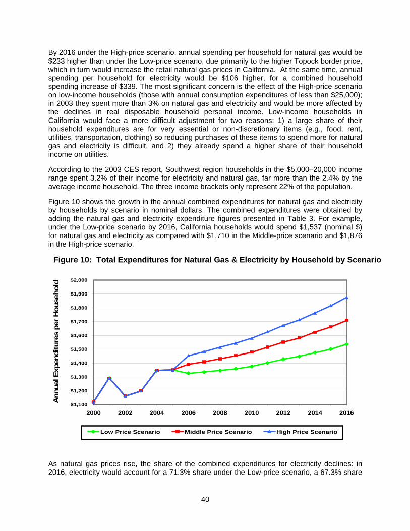
40

By 2016 under the High-price scenario, annual spending per household for natural gas would be $233 higher than under the Low-price scenario, due primarily to the higher Topock border price, which in turn would increase the retail natural gas prices in California. At the same time, annual spending per household for electricity would be $106 higher, for a combined household spending increase of $339. The most significant concern is the effect of the High-price scenario on low-income households (those with annual consumption expenditures of less than $25,000); in 2003 they spent more than 3% on natural gas and electricity and would be more affected by the declines in real disposable household personal income. Low-income households in California would face a more difficult adjustment for two reasons: 1) a large share of their household expenditures are for very essential or non-discretionary items (e.g., food, rent, utilities, transportation, clothing) so reducing purchases of these items to spend more for natural gas and electricity is difficult, and 2) they already spend a higher share of their household income on utilities.

According to the 2003 CES report, Southwest region households in the $5,000–20,000 income range spent 3.2% of their income for electricity and natural gas, far more than the 2.4% by the average income household. The three income brackets only represent 22% of the population.

Figure 10 shows the growth in the annual combined expenditures for natural gas and electricity by households by scenario in nominal dollars. The combined expenditures were obtained by adding the natural gas and electricity expenditure figures presented in Table 3. For example, under the Low-price scenario by 2016, California households would spend $1,537 (nominal $) for natural gas and electricity as compared with $1,710 in the Middle-price scenario and $1,876 in the High-price scenario.

Figure 10: Total Expenditures for Natural Gas & Electricity by Household by Scenario

$1,100

$1,200

$1,300

$1,400

$1,500

$1,600

$1,700

$1,800

$1,900

$2,000

2000 2002 2004 2006 2008 2010 2012 2014 2016

Ann

ual E

xpen

ditu

res

per H

ouse

hold

Low Price Scenario Middle Price Scenario High Price Scenario

As natural gas prices rise, the share of the combined expenditures for electricity declines: in 2016, electricity would account for a 71.3% share under the Low-price scenario, a 67.3% share

41

in the Middle-price scenario, and a 64.1% share in the High-price scenario. Electricity accounts for approximately two-thirds of the combined expenditure, so that as electricity prices rise due to higher natural gas prices, consumers will reduce their use of it to lower spending. It is also likely that the percent increase in the residential retail electricity price will be less than the percent increase in the residential retail natural gas price.

Table 3 presents average household income levels in nominal dollars. The percent decreases in nominal average household income by 2016 under the Middle- and High-price scenarios shown in Table 3 are less than the corresponding percent declines for real household income shown in Table 2, indicating that the higher nominal energy prices result in higher inflation and eventually in lower real (or inflation-adjusted) levels of economic activity.

The increases in spending by households presented in Table 3 were based on the retail natural gas and electricity prices in California forecast by the Global Insight energy model, which in turn were based on the three price scenarios. A potential concern is that the future levels of retail electricity prices in California could be higher than we have forecast because of the use of natural gas by industrial customers who co-generate electric power and sell it to State utilities. The EIA divides the amount of natural gas used by industrial customers for producing steam and co-generating electricity into industrial demand and electric generation demand: the CEC assigns the entire amount of this natural gas use to electric generation demand. The cogeneration issue is significant because a substantial share of the electric power produced in California comes from co-generators. The relationship between the natural gas demand by co-generators and the effect on electricity prices is discussed in more detail below in the Merchant Power Company section of Appendix B. It is difficult to estimate how much higher retail electricity prices could be under the three price scenarios due to this pass-through; at the same time the higher electricity prices would provide an additional incentive for customers to further reduce their consumption of electricity. For these reasons, we conclude that increases in spending by households for electricity presented in Table 3 are conservative. For example, if by 2016 retail residential electricity prices in the High-price scenario were 10% higher than we have forecast, annual spending for electricity would increase from $1,203 up to as much as $1,323; the actual increase in annual electricity spending would be less than this figure as annual household consumption of electricity would rise less than 10% because of the higher price.

Figure 11 shows the consumption of natural gas and electricity in MMBtu per household by scenario. The figure clearly shows that higher retail natural gas and electricity prices would result in California households reducing the amount of energy they use in order to lower spending.

Commercial

Table 1 presents the changes in purchases of natural gas under the three scenarios for commercial customers. The table shows that under the Middle scenario in 2016, purchases of natural gas (in nominal dollars) by commercial customers would be approximately $3.5 billion, compared to only $2.7 billion under the Low-price scenario, but less than the $4.3 billion spent under the High-price scenario. These direct effects generate the changes in total economic activity presented above in Table 2 and in the tables in Appendix A.

Employment in the PSP sectors would not experience the large percentage change in employment as does manufacturing, but the absolute numbers of jobs that will be eliminated would be far higher. Appendix Table A-2 demonstrates that by 2016, employment in the PSP sectors in the Middle-price scenario would account for 67,400 fewer jobs than would employment in the Low-price scenario, or 69% of the total job loss that year.

42

Figure 11: Consumption of Natural Gas & and Electricity per Household by Scenario

61.0000

62.0000

63.0000

64.0000

65.0000

66.0000

67.0000

68.0000

69.0000

70.0000

2000 2002 2004 2006 2008 2010 2012 2014 2016

MM

Btu

s/H

ouse

hold

/Yea

r

Low Price Scenario Middle Price Scenario High Price Scenario

Similarly, under the High-price scenario, employment in the private, services-producing sectors in 2016 would be 108,000 fewer jobs than in the Low-price scenario, comprising 66% of the total job loss.

Industrial

The employment impacts in the manufacturing sector, the economic sector where most of the industrial end users of natural gas are found, were covered above. Table 1 above provides estimates of direct spending for natural gas by industrial customers, and shows that, on average, the amount spent for natural gas by industrial customers is about 2.5 times greater than the amount spent by commercial customers. Under the High-price scenario, industrial customers are projected to spend approximately $10.8 billion (nominal dollars) for natural gas in 2016, well more than the $8.8 billion and $6.6 billion seen in the Middle- and Low-price-scenarios.

Government

Government employment would be largely unaffected under the three price scenarios. The first two categories barely registered a change in either scenario, only the military which has the option of closing bases and relocating elsewhere was affected. Appendix Table A-2 shows that under the High-price scenario by 2016, total government employment would be only 8,100 fewer jobs than under the Low-price scenario.

43

Electric Generation

One of the primary direct effects of alternative natural gas prices will be on the cost of generating electricity because California generates a much higher share of its electricity using natural gas than does the rest of the county. According to the EIA, in 2001, just more than 49.0% of electric power generated in California was produced by burning natural gas; only 1.0% was made by burning coal, as compared with U.S. shares of 16.4% and 51.2%, respectively. Since California imports about 20% of its energy, natural gas’s share of total electric power used in California is about 41.0% (CEC, 2005 Integrated Energy Policy Report). Higher natural gas prices will directly raise the price of generating electricity, requiring businesses and households to pay more to obtain it and providing them an incentive to use less of it.

We estimate that by 2016, total purchases of natural gas by California’s electric utilities used in generating electric power under the Middle-price and High-price scenarios will be $6.5 billion and $8.3 billion, substantially higher than the $4.6 billion under the Low-price scenario. The higher prices for natural gas will be reflected in higher retail electricity prices, leading to the negative impacts on households noted above.

Impacts in Northern and Southern California At the request of the Advisory Committee, Global Insight estimated the economic impact for Northern and Southern California, with the former generally aligned with Pacific Gas and Electric’s natural gas service area as far south as the southern boundary of Tulare County. These two areas are shown in Figure 12, and were based on the current service areas for the major natural gas companies that provide retail service in the state.

Southern California was defined as 100% of the nine counties in yellow: Imperial, Los Angeles, San Luis Obispo, Santa Barbara, Orange, San Diego, Ventura, Riverside, and San Bernardino; and portions of the following counties in brown: (based on household coverage): Kern County (Bakersfield) 50%; Tulare (Visalia-Porterville) 95%; Kings (Hanford) 80%; Fresno, 5%. The shares of households served in counties where more than one company provides natural gas services were estimated using information provided by members of the Advisory Committee. The remaining part of the state was defined as Northern California, and consists of all the counties in white and two of three shown in brown.

Employment

Southern California contains 9.1 million of the 15 million non-farm jobs in California (61% of the total); so it is unsurprising that higher natural gas prices would eliminate more jobs in the lower half of the state than in the less-populated northern half. In comparing the changes between the High- and Low-price scenarios, we forecast that 101,400 of the total statewide decline in employment of 163,300 jobs by 2016 would occur in Southern California, with the remaining 61,900 jobs lost in Northern California. The major reason that employment impacts would be more significant in Southern California is that it has high shares of statewide employment in a number of sectors, especially in the manufacturing, where the impact of the natural gas prices would be the most significant. In other words, Southern California is over-represented in some major natural-gas intensive sectors, and under-represented in others that are much less dependent on natural gas.

For most economic sectors, the shares of statewide employment in Southern California range from 60–70%, roughly in line with regional shares of the California population and total employment. We identified nine sectors for which shares of statewide employment exceeded

44

Figure 12: Northern and Southern California Study Areas

70%, indicating that they are over-represented in Southern California. All nine of these sectors are in manufacturing, due in large part to the broad manufacturing base of the Los Angeles region, and especially because of the heavy concentration of defense and aerospace firms in southern California. By contrast, some employment sectors are very under-represented in Southern California, indicating that they are likely over-represented in Northern California. We identified eight sectors in Southern California for which shares of statewide employment were less than 60%. Companies in these eight sectors prefer locations in Northern California over those in Southern California. The most obvious of these is beverage manufacturing, as 80% of its statewide employment is in Northern California, which is no surprise: Napa and surrounding counties dominate the wine industry in California. The State Government employment share is also high, as the State Capitol of Sacramento is located in the northern half of the state. Finally, industries related to wood products are concentrated in the northern part of the state, whereas computer firms are concentrated in Silicon Valley.

45

Gross State Product

As natural gas prices rise in the Middle- and High-price scenarios, the levels of real GSP declines in both Northern and Southern California. As with employment impacts, the absolute and percentage changes are determined the economic structure of each region. Based on the over- and under-represented economic sectors in Southern California, the level of real GSP, or real value-added output, likely would be more adversely affected in Southern California than in Northern California by high, sustained natural gas price levels.

We estimate that in 2016, the difference in the level of real GSP in southern California between the High-price and Low-price scenarios would be about $20.6 billion, or about 67% of the statewide decline of $30.4 billion shown above in Table 2, with the drop in Northern California being much smaller at about $9.8 billion. Our analysis showed that the percent differences in real GSP between the Middle-price and Low-price scenarios and between the High-price and Low-price scenarios would be slightly higher in Southern California than in Northern California.

Finally, the decrease in real GSP per job eliminated would be noticeably higher in Southern California. We forecast that in 2016, real GSP would decline $203,200 per job when comparing the High-price scenario to the Low-price scenario, as compared with only $159,400 per job in Northern California. As a result, the percentage declines in real personal incomes would be higher in Southern California.

Results of Other Studies We found one other recent study which also measured the economic impact of the higher natural gas prices on the state of California (“High Natural Gas Prices Need Not Cook California’s Economy: The Case for Liquefied Natural Gas,” Professor Philip Romero, Lindquist College of Business, University of Oregon, April, 2005). The study used elasticities between the levels of total GSP, employment, and household income, and the price level of natural gas to estimate statewide economic impacts of changes in natural gas prices. There were differences in the methodologies between Professor Romero’s study and that conducted by Global Insight: his analyzed the entire economy while we used a sector-by-sector approach. In addition, differences in the price levels of natural gas were considered in the two studies. Even with these differences, we found that Professor Romero’s study provided good, initial estimates of the statewide economic impacts of changes in California natural gas prices, and that his results were generally consistent with ours. We were able to extend his analysis by using our econometric models as described above, taking advantage of their sectoral detail. Professor Romero’s study found that a 10% reduction in natural gas prices would have the following impacts when using a top-down approach:

• An increase in California’s total 2005 GSP of between $.96 billion (+0.067%) and $3.45 billion (+0.024%)

• An increase in employment of between 11,500 and 41,500 jobs • An increase in total California household income of between $0.38 billion and $1.38

billion Similarly, a 10% reduction in natural gas prices would have the following impacts when using a bottom-up approach:

46

• An increase in California’s total 2005 GSP of $2.3 billion (+0.16%) • An increase in employment of 27,700 jobs • An increase in total California household income of $0.92 billion

Finally, a 20% reduction in natural gas prices would have the following impacts when using a bottom-up approach:

• An increase in California’s total 2005 GSP of $4.6 billion (+0.32%) • An increase in employment of 55,300 jobs • An increase in total California household income of $1.84 billion

By way of comparison, the differences between the prices in Middle scenario and those for the High and Low scenarios in our study start at just less than 14.0% in 2006 and reach 33.3% by 2016. Professor Romero’s study also noted that economic impacts of lower natural gas prices on the U.S. economy, on a proportional basis, would be about 3/4 those on the California economy—again, as consistent with our analysis that showed the California economy is more dependent on the price of natural gas than is the U.S. economy.

47

SUMMARY

Level of State-wide Economic Activity Falls with Higher Prices Sustained, higher annual natural gas prices would have an adverse impact on the economy of California. Higher wholesale natural gas prices, as represented by the Topock border prices used in three price scenarios considered in this study, would result in higher retail natural gas prices for the major end-user groups (e.g., residential, commercial, industrial, and electric generation), which would in turn increase the amount of their energy expenditures and their costs of production. Over time, businesses and households would continually adapt to sustained, higher natural gas prices in a variety of ways intended to use natural gas more efficiently, and to reduce costs in other areas to offset as much as possible the higher expenditures for natural gas. The very large size of the California economy means sizeable declines in absolute terms in the levels of economic activity that would occur by 2010 and 2016 under the Middle-price and High-price scenarios, when compared with those seen in the Low-price scenarios. For example, we estimate that by 2106, under the High-price scenario, total real GSP (in constant 2000$) would be $30.4 billion lower than under the Low-price scenario (the corresponding decline in nominal GSP would be about $42.2 billion). Similarly, we estimate that by 2016, total employment in California under the Middle-price and High-price scenarios would be 97,700, and 163,300 jobs less than under the Low-price scenario.

On a percentage basis, the declines in the aggregate levels of economic activity, as measured by total employment, total GSP, and total personal income, would be small, averaging 1.0–1.3% under the High-price scenario by 2016. Proportional economic impacts would be noticeably higher in the manufacturing sector, however, where we find that by 2016, employment and real GSP under the High-price scenario would be 2.1% and 3.3% less than the levels seen in the Low-price scenario; the percent decline in industrial production would be about the same. The interviews we conducted with major industrial and commercial users of natural gas, including electric generators, indicated clearly that California companies have been making adjustments to higher natural gas prices for some years now, especially since the utility crisis of 2001–02. They said that many of the more easily achievable costs savings had already been captured, especially in the manufacturing sector, so that future cost reductions will need to be obtained from a variety of measures in addition to eliminating jobs.

The total state-wide economic impacts would be generated by the direct effect of each price scenario, or the amount spent by final users to buy natural gas. Under the High-price scenario, total expenditures for natural gas by 2016 (in real or constant year 2000 dollars) by the four major end-user groups would be about $23.2 billion ($33.2 billion in nominal terms), or $9 billion higher than under the Low-price scenario ($13 billion higher in nominal terms). The result of the higher spending on natural gas is that real GSP under the High-price scenario in 2016 would be $30.4 billion less than in the Low-price scenario, yielding a real value-added multiplier of just less than 3.4.

Households Affected by Higher Energy Expenditures and Lower Incomes California households would be affected by sustained higher natural gas prices in several ways: 1) by the declines in the levels of economic activity, especially the job losses and the corresponding drop in wage and salary income; 2) by higher spending for natural gas and

48

electricity, which reduces the money available to purchase other goods and services; and 3) by higher inflation resulting from the higher nominal prices for energy, which in turn lowers real disposable personal income. In nominal terms, we estimate that combined expenditures for natural gas and electricity by 2016 would total $1,876 per household under the High-price scenario, comprised of $1,203 for electricity and $673 for natural gas. Finally, the percent declines in the wage and salary earnings component of real total personal income under the Middle-price and High-price scenarios would be higher than the percent drops in total real personal income due to the combined effects of lower employment and higher price levels.

Marginal Impacts Decline as Natural Gas Prices Rise The study shows that the marginal economic impacts would decline as natural gas prices rise, and conversely, that the marginal economic benefits would get progressively larger as natural gas prices fall. The marginal economic impact is the change in the level of economic activity (e.g., employment, income, GSP) resulting from a direct economic effect, in this case an increase or decrease in the price of natural gas. The existing price level before a change occurs determines the size of the marginal economic impact—if the natural gas price level is already high, a further rise of 1% would have a smaller, negative, marginal economic impact than a 1% increase from a low price level. For example, the number of jobs lost for each 1% price increase between the Middle- and High-price scenarios would be less than the number lost for each 1% price drop between the Low- and Middle-price scenarios. The reverse would also occur; the increase in employment for each 1% price decline between the High- and Middle-price scenarios would be less than the employment increase for each 1% price decline between the Middle- and Low-price scenarios. In other words, the marginal economic effects of natural price movements are asymmetrical because they depend on the price level (e.g., high or low) that exists when prices change.

The decline in marginal impacts as prices increase means that up to a certain price level, most of the adjustments that can be made to reduce energy costs will have been implemented and the savings realized, so that above this price there is little more that can be done to further reduce energy use without also lowering production levels (i.e., no more workers can be laid off, energy use cannot be reduced any further, and all the energy-efficient equipment required has been installed). The energy cost savings that can be realized will become smaller, and the marginal expenditures required to obtain them will become increasingly higher. With falling prices, such as from the High- to the Low-price scenario, the reduction in natural gas and electricity expenditures are immediately realized as additional revenues, enabling businesses to lower prices, increase profits, or invest the freed-up funds in more productive ways. Lower costs in turn would make key California industries more competitive in time, resulting in lower inflation and leading to subsequent increases in real output and incomes.

The asymmetry or declining marginal economic effects of rising natural gas prices were identified by estimating implicit employment elasticities, which were defined as the percent decline in employment for each 1% increase in natural gas prices between two scenarios (i.e., from the Low-price to the Middle-price scenario, and from the Low-price to the High-price scenario).

Impacts of Higher Natural Gas Prices Increase over Time Our forecasts for the three price scenarios clearly showed the negative, economic impacts of sustained, high natural gas increase over time. Table 2 above and the detailed tables in Appendix A consistently show larger absolute differences in real dollars, and on a percentage basis, in 2016 than in 2010 when analyzing differences in the levels of economic activity

49

between the High-price and Low-price scenarios, and between the Middle- and Low-price scenarios. For example, the differences in total employment in 2010 between the High- and Low-price scenarios would be -109,800 jobs and -0.7%; by the 2016 the corresponding differences would rise to -163,300 jobs and -1.0%. Similar trends exist for both real GSP and real personal income. The primary reason is that the differences in the price levels across the three scenarios in real terms widens over time as shown above in Figure 5, although the numerical difference between the Topock border and Henry Hub prices stays constant over time. For example, as prices continue to increase under the High-price scenario relative to those for the other two scenarios, businesses and households continue to make adjustments in the face of continuing, high natural gas prices in order to reduce their energy costs. Some of these adjustments, such as reducing output, eliminating jobs, and shifting operations to lower-cost locations reduce the level of economic activity in California as measured by real GSP. At the same time, continuing high natural gas prices decrease the competitiveness of California’s natural-gas intensive industries, and lower real disposable incomes as energy prices remain high. The process of continual adjustment means that the levels of economic activity by 2016 under each scenario will be the cumulative result of all the actions that were made by firms and households during the preceding decade.

California is More Sensitive to High Natural Gas Prices than the U.S. Economy The study showed that the California economy is slightly more sensitive to higher natural gas prices than is the U.S. economy. We corrected for differences in the levels of wholesale natural gas prices in the U.S. and California under the three scenarios by estimating implicit elasticities for such key aggregate indicators such as GDP/GSP, employment, and real income. These elasticities indicated that a 1% increase in the wholesale price of natural gas in the United States would generally have a smaller, adverse impact in percentage terms than a 1% increase in wholesale natural gas prices in California. The California economy is more sensitive to the price of natural gas than is U.S. economy for several reasons: 1) its major natural gas-using sectors—notably chemicals, plastic and rubber products, non-metallic minerals (i.e., glass and cement), primary and fabricated metals, and food—obtain higher shares of their energy inputs on a Btu basis from natural gas than do these same sectors at the national level; and 2) more than 49% of the electric power generated in California is produced by burning natural gas, so that rising natural gas prices increase the retail prices of electricity for all major end-user groups, and the negative effects of these higher costs ripple throughout the economy. Higher electricity prices are also significant because California households currently spend, on average, about $1.91 for electricity for every $1 spent for natural gas.

Structure of California’s Economy would be Unaffected A number of economic forces, both domestic and global, have been and will continue to produce changers in the structures of both the U.S. and California economies. Many of these factors are well-known and widely studied, including the continuing relative decline of the manufacturing sector and the increasing importance of the services providing sectors; global factors such as the rise of China, India and other Asian economies; off-shoring; current and future trade agreements such as NAFTA; fiscal and monetary policies of major trading countries and blocks such as the EU; competitive advantages and disadvantages of the California economy such as high labor and housing costs in its largest MSAs, regional migration trends of household and businesses in the western United States, the California business tax, environmental and energy policies, etc. Higher sustained natural gas prices, when considered along with all of these other factors, would have little, if any, impact on the structure of the

50

California economy. We do find that both the Middle-price and High-price scenarios would slightly increase the rate of long-term decline in the manufacturing sector, but this trend will continue regardless of the future price of natural gas.

51

APPENDIX A: DETAILED ECONOMIC IMPACTS IN CALIFORNIA

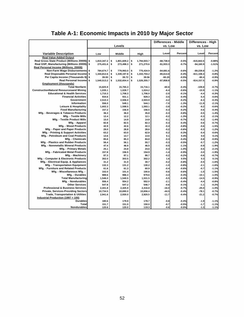
52

Table A-1: Economic Impacts in 2010 by Major Sector

Variable Description Low Middle High Level Percent Level PercentReal Value-Added Output

Real Gross State Product (Millions 2000$) 1,810,347.2$ 1,801,609.2$ 1,794,503.7$ -$8,738.0 -0.5% -$15,843.5 -0.88%Real GSP, Manufacturing (Millions 2000$) 275,431.6$ 273,498.3$ 271,270.6$ -$1,933.3 -0.7% -$4,160.9 -1.51%

Real Personal Income (Millions, 2000$)Non-Farm Wage Disbursements 784,674.7$ 779,993.0$ 775,434.9$ -$4,681.6 -0.6% -$9,239.8 -1.2%

Real Disposable Personal Income 1,344,812.6$ 1,339,197.8$ 1,333,704.2$ -$5,614.8 -0.4% -$11,108.4 -0.8%Per Capita Income (Thousands $) 39.93$ 39.72$ 39.56$ -$0.20 -0.5% -$0.4 -0.9%

Real Personal Income 1,540,513.2$ 1,532,654.4$ 1,526,355.7$ -$7,858.8 -0.5% -$14,157.5 -0.9%Employment (thousands)

Total Nonfarm 15,825.9 15,765.3 15,716.1 -60.6 -0.4% -109.8 -0.7%ConstructionNatural Resourcesand Mining 1,035.1 1,028.7 1,024.2 -6.4 -0.6% -10.9 -1.1%

Educational & Health Services 1,710.3 1,708.3 1,706.0 -2.0 -0.1% -4.4 -0.3%Financial Activities 934.6 931.1 929.3 -3.5 -0.4% -5.4 -0.6%

Government 2,510.3 2,506.0 2,503.9 -4.2 -0.2% -6.3 -0.3%Information 556.0 549.1 544.1 -7.0 -1.3% -11.9 -2.1%

Leisure & Hospitality 1,602.3 1,598.5 1,593.1 -3.8 -0.2% -9.2 -0.6%Food Manufacturing 157.2 156.9 156.5 -0.3 -0.2% -0.6 -0.4%

Mfg. - Beverages & Tobacco Products 36.3 36.0 35.8 -0.3 -0.8% -0.5 -1.4%Mfg. - Textile Mills 12.4 12.2 12.1 -0.2 -1.3% -0.3 -2.1%

Mfg. - Textile Product Mills 15.0 14.9 14.8 -0.1 -0.7% -0.2 -1.4%Mfg. - Apparel 82.8 82.5 82.3 -0.3 -0.4% -0.6 -0.7%

Mfg. - Wood Products 42.9 42.6 42.3 -0.4 -0.8% -0.6 -1.5%Mfg. - Paper and Paper Products 29.0 28.8 28.6 -0.2 -0.6% -0.3 -1.2%

Mfg. - Printing & Support Activities 63.2 63.0 62.8 -0.2 -0.3% -0.4 -0.6%Mfg. - Petroleum and Coal Products 13.6 13.7 13.6 0.1 0.4% 0.0 0.1%

Mfg. - Chemicals 85.6 85.3 84.8 -0.3 -0.4% -0.8 -0.9%Mfg. - Plastics and Rubber Products 56.4 56.1 55.7 -0.3 -0.5% -0.7 -1.2%Mfg. - Nonmetallic Mineral Products 47.4 46.9 46.5 -0.5 -1.1% -0.9 -1.9%

Mfg. - Primary Metals 25.1 24.8 24.6 -0.3 -1.0% -0.5 -2.1%Mfg. - Fabricated Metal Products 157.8 156.5 154.9 -1.4 -0.9% -3.0 -1.9%

Mfg. - Machinery 87.3 87.1 86.7 -0.2 -0.2% -0.6 -0.7%Mfg. - Computer & Electronic Products 302.0 303.5 302.2 1.6 0.5% 0.3 0.1%

Mfg. - Electrical Equip. & Appliances 31.2 31.0 30.7 -0.2 -0.8% -0.5 -1.6%Mfg. - Transportation Equipment 132.3 131.2 130.2 -1.0 -0.8% -2.1 -1.6%

Mfg. - Furniture and Related Products 61.6 61.3 60.9 -0.4 -0.6% -0.7 -1.1%Mfg. - Miscellaneous Mfg. - 102.0 101.4 100.6 -0.6 -0.6% -1.5 -1.5%

Mfg. - Durables 989.6 986.3 979.6 -3.4 -0.3% -10.1 -1.0%Total Manufacturing 1,546.0 1,540.5 1,531.5 -5.5 -0.4% -14.5 -0.9%Mfg. - Nondurables 556.4 554.2 552.0 -2.1 -0.4% -4.4 -0.8%

Other Services 547.8 547.2 546.7 -0.6 -0.1% -1.1 -0.2%Professional & Business Services 2,441.8 2,425.9 2,416.8 -16.0 -0.7% -25.0 -1.0%

Private, Services-Providing Sectors 10,734.5 10,690.0 10,656.4 -44.5 -0.4% -78.1 -0.7%Trade, Transportation & Utilities 2,941.6 2,930.0 2,920.5 -11.7 -0.4% -21.2 -0.7%

Industrial Production (1997 = 100)Durables 180.6 179.9 178.7 -0.8 -0.4% -1.9 -1.1%

Total 151.7 151.0 150.0 -0.7 -0.5% -1.7 -1.1% Nondurables 120.6 120.0 119.3 -0.6 -0.5% -1.3 -1.1%

LevelsDifferences - Middle

vs. LowDifferences - High

vs. Low

53

Table A-2: Economic Impacts in 2016 by Major Sector

Variable Description Low Middle High Level Percent Level PercentReal Value-Added Output

Real Gross State Product (Millions 2000$) 2,327,620.0$ 2,310,660.1$ 2,297,179.6$ -$16,959.95 -0.7% -$30,440.4 -1.3%Real GSP, Manufacturing (Millions 2000$) 395,834.0$ 389,055.4$ 382,780.4$ -$6,778.65 -1.7% -$13,053.7 -3.3%

Real Personal Income (Millions, 2000$)Non-Farm Wage Disbursements 921,978.2$ 914,184.4$ 906,631.9$ -$7,793.9 -0.8% -$15,346.3 -1.7%

Real Disposable Personal Income 1,593,157.1$ 1,584,649.4$ 1,575,833.9$ -$8,507.7 -0.5% -$17,323.2 -1.1%Per Capita Income (Thousands $) 44.6$ 44.4$ 44.1$ -$0.3 -0.6% -$0.5 -1.1%

Real Personal Income 1,844,797.2$ 1,834,235.7$ 1,824,048.5$ -$10,561.6 -0.6% -$20,748.8 -1.1%Employment (thousands)

Total Nonfarm 17,083.7 16,986.0 16,920.4 -97.67 -0.6% -163.3 -1.0%ConstructionNatural Resourcesand Mining 1,158.4 1,148.6 1,143.6 -9.87 -0.9% -14.8 -1.3%

Educational & Health Services 1,808.0 1,803.6 1,799.7 -4.41 -0.2% -8.2 -0.5%Financial Activities 1,002.3 997.3 994.6 -5.01 -0.5% -7.7 -0.8%

Government 2,654.1 2,648.9 2,646.1 -5.23 -0.2% -8.1 -0.3%Information 613.1 605.9 602.2 -7.26 -1.2% -11.0 -1.8%

Leisure & Hospitality 1,713.0 1,708.2 1,704.8 -4.80 -0.3% -8.2 -0.5%Food Manufacturing 161.1 160.0 159.3 -1.04 -0.6% -1.8 -1.1%

Mfg. - Beverages & Tobacco Products 36.1 35.8 35.7 -0.29 -0.8% -0.5 -1.3%Mfg. - Textile Mills 13.0 12.7 12.5 -0.31 -2.4% -0.5 -3.8%

Mfg. - Textile Product Mills 15.6 15.3 15.1 -0.26 -1.7% -0.4 -2.8%Mfg. - Apparel 90.6 90.2 89.7 -0.48 -0.5% -0.9 -1.0%

Mfg. - Wood Products 48.2 47.6 47.2 -0.59 -1.2% -1.0 -2.2%Mfg. - Paper and Paper Products 27.8 27.4 27.1 -0.38 -1.4% -0.7 -2.4%

Mfg. - Printing & Support Activities 60.4 60.0 59.6 -0.43 -0.7% -0.8 -1.3%Mfg. - Petroleum and Coal Products 10.9 11.0 10.8 0.11 1.0% 0.0 -0.4%

Mfg. - Chemicals 92.1 91.4 90.5 -0.73 -0.8% -1.6 -1.7%Mfg. - Plastics and Rubber Products 53.9 53.1 52.3 -0.75 -1.4% -1.6 -2.9%Mfg. - Nonmetallic Mineral Products 46.1 45.1 44.3 -0.99 -2.2% -1.8 -3.9%

Mfg. - Primary Metals 24.5 23.9 23.5 -0.51 -2.1% -1.0 -3.9%Mfg. - Fabricated Metal Products 163.8 161.4 158.8 -2.43 -1.5% -5.0 -3.1%

Mfg. - Machinery 92.5 92.0 91.1 -0.43 -0.5% -1.3 -1.4%Mfg. - Computer & Electronic Products 302.0 301.2 298.3 -0.82 -0.3% -3.7 -1.2%

Mfg. - Electrical Equip. & Appliances 29.7 29.3 28.8 -0.43 -1.4% -0.9 -3.1%Mfg. - Transportation Equipment 130.0 127.6 125.5 -2.44 -1.9% -4.5 -3.5%

Mfg. - Furniture and Related Products 60.9 60.3 59.7 -0.66 -1.1% -1.3 -2.1%Mfg. - Miscellaneous Mfg. - 109.8 108.5 106.7 -1.26 -1.1% -3.1 -2.8%

Mfg. - Durables 1,007.5 996.9 983.8 -10.56 -1.0% -23.6 -2.3%Total Manufacturing 1,574.8 1,559.6 1,542.3 -15.18 -1.0% -32.5 -2.1%Mfg. - Nondurables 567.3 562.7 558.4 -4.62 -0.8% -8.9 -1.6%

Other Services 572.7 571.8 571.1 -0.90 -0.2% -1.6 -0.3%Professional & Business Services 2,861.5 2,838.8 2,827.1 -22.73 -0.8% -34.4 -1.2%

Private, Services-Providing Sectors 11,696.4 11,628.9 11,588.4 -67.42 -0.6% -108.0 -0.9%Trade, Transportation & Utilities 3,125.7 3,103.4 3,088.9 -22.31 -0.7% -36.9 -1.2%

Industrial Production (1997 = 100)Durables 263.2 260.5 257.0 -2.68 -1.0% -6.1 -2.3%

Total 203.2 201.2 198.6 -2.02 -1.0% -4.6 -2.3% Nondurables 144.1 142.9 141.4 -1.14 -0.8% -2.7 -1.9%

LevelsDifferences - High vs.

LowDifferences - Middle vs.

Low

54

APPENDIX B: INTERVIEWS WITH ENERGY-INTENSIVE INDUSTRIES

Background The major public utilities in California are examining the impact of rising energy prices on the California economy. Through its proprietary economic models, and with price scenarios designed by the California Advisory Group, Global Insight prepared a detailed study of how natural gas and electricity prices will affect the economic performance of the state. The economic impact of rising energy prices will be felt particularly in those industries that require the highest amount of energy in production. Along with the results of U.S. and California economic and energy system models, Global Insight has interviewed key energy-intensive companies within California to ascertain the real-life situation of those companies most affected by rising prices within the state. Figure B-1 presents a classification of industries based on their sensitivity to energy prices.

Figure B-1: Energy Price Sensitivity Matrix

Moderate Ability Difficult Abilityto Pass on Costs to Pass on Costs

Retail Trade Chemical ManufacturingHigh Tourism Pulp and PaperEnergy Petroleum Refining Iron and SteelIntensity Resource Extraction Aluminum

Glass, CementEnvironmenal Technology

BiosciencesFood

Low Banking and Finance Computers and ElectronicsEnergy Business Services ConstructionIntensity Other Services Transportation Equipment

Manufacturing - FabricationMultimedia

Public AdministrationTelecommunications

Wholesale Trade

55

Global Insight interviews of California companies focused upon those that have high energy intensity and difficulty in passing on the rising costs of energy to their customers. Such industries as Petroleum Refining, Chemicals, Paper, Metals, Glass, Cement, Resource Extraction and Food account for most of the energy use in the industrial sector. The Energy Price Sensitivity Matrix upper right quadrant indicates the types of industries most likely to be affected by rising energy costs.

The results of the interviews are used to interpret the results of the scenarios and model-based analysis.

Overview Rising energy costs and national recessions have caused large losses of employment in California manufacturing industries in the past. In 2000–04, California lost more than 320,000 manufacturing jobs from a combination of price spikes, recession, and industry trends. One-third of the losses were in the computer industry, while apparel, fabricated metals, machinery, and transportation equipment industries also experienced significant employment losses. A future episode of high natural gas prices could also impact the California economy and energy-intensive industries.

The share of U.S. manufacturing commanded by California is slightly less than the state share of the total economy despite a long history of industry closing up shop and leaving the state. Energy has been part of the impetus to energy-intensive industries, such as basic chemicals, steel, aluminum, and paper-reducing operations in California. Growth in less energy-intensive areas, however, such as information technology and biotechnology has matched the loss of other industries in the past five years.

The reasons why industries stay, leave, flourish, or decline are usually unique to their individual process or circumstances. Many agricultural industries are located in California for special reasons such as the wine industry for its unique growing climate. For one of the most energy-intensive industries, petroleum refining, California is nearly self-sufficient, in part because of very special product standards that exceed those that out-of-state refiners can meet, and because of the large size of the market, making it feasible to locate facilities dedicated to the California market in the State. Also limiting losses of industrial demand is the fact that many energy-intensive industries such as ammonia, basic organic chemicals, aluminum smelters, and steel mills have either never been located in California or have already closed during prior episodes of high natural gas prices. As of the fourth quarter of 2005, the California manufacturing sector was still very large with about 1.539 million jobs, and it produced $193.8 billion annually in manufacturing Gross State Product, about 12.3 % of the U.S. total.

In many ways, California is a world-scale economy with total value added that would place it ahead of all but seven countries in the world. As it accounts for 13.3% of the U.S. GDP, California is also greatly affected by national trends. The United States is still the leader in manufacturing, with 23.8% of the world total value added according to the World Bank. This output is created by more than 100,000 companies with more than 20 employees in the United States. Also, many foreign companies, such as Toyota and Honda, manufacture their products in the United States for the NAFTA market.

More importantly, an enormous variety of U.S. manufacturers have stayed put in the United States despite globalization. Despite very high labor costs and rising energy costs, U.S. and California industries have many strong advantages.

56

• The U.S. is the world leader in manufacturing; as such, many local customers are best served by U.S.-based firms.

• The U.S. food industry maintains significant advantages in quality and low cost versus that of other nations. U.S. agriculture is by far the most productive in the world, and benefits from a wonderful climate.

• Globalization from reduced barriers to trade has allowed for the expansion of U.S. export-oriented industries. Manufacturing exports are rising faster than are manufacturing outputs.

• U.S. productivity is very high as compared with that of developing countries. Also, the United States has an abundant supply of labor from immigration, and sustained 0.8% population growth.

• The U.S. leads the world in new product development and commercialization for leading growth sectors such as information technology and biotechnology.

These advantages translate into several areas of success for California including Silicon Valley and the wine industry. Management and innovation are among the reasons for the success of U.S. manufacturing, as measured by retention of its share of world output. Companies that are successful exhibit many of the following traits:

• Chief executives grew up with the company and have an unusual attachment to the products they make.

• Innovation is necessary. Engineers and designers are constantly altering company products in ways that are not easily imitated by lower-priced, foreign competitors.

• Cost-saving measures, such as productivity improvement, automation, outsourcing to specialty firms, and improving energy efficiency create advantages for U.S. industry.

U.S. manufacturing is under pressure because:

• U.S. energy costs and especially those of California are among the highest in the world as compared with coal-based electricity generators in China and subsidized oil and gas prices in other countries. Energy intensive industries continue to struggle with a substantial shutdown of ammonia, aluminum, and ethylene plants in recent years.

• Also, U.S. labor costs are very high, as befits their productivity; however, state-run programs, such as workmen's compensation, demand exorbitant costs as compared with those of international competitors.

• Environmental rules are extremely restrictive on operations, often eliminating the possibility of fuel-switching and also requiring massive investments in pollution control. Recycling laws in California create additional industry burdens that are not shared in other locales.

• Globalization from reduced barriers to trade allows companies to relocate abroad and export back to the United States.

• High-grade electric motors, flat-screen computer panels, and some specialty steels are no longer made in the United States because production costs are lower in other countries.

• Off-the-shelf commodities are purchased from the lowest qualified bidder. Metal foundries are moving out of the U.S. and California. During times of low energy costs there is a gradual increase in U.S. content, but in bad times, this can plummet.

57

Interviews of California Companies The interviews include a range of companies operating in California that have widely differing circumstances but also specific energy cost issues in their operations. The subjects of the interviews were extended to include non-manufacturing sectors, such as power production. These sectors included the Department of Water and Power, which is involved in procuring electric power under long-term contracts and has a large exposure to natural gas prices. Representatives of the engineering procurement, construction, and the energy efficiency equipment supplier industries were also interviewed.

Energy Efficiency An attractive option for California companies is investment in improved energy efficiency; however, this option is slow-going, according to Alzeta Corp. Energy use per unit of output is difficult to change for existing products and plants. With energy prices in other locales much lower than in the United States and California, even a substantial savings in energy consumption can only offset a small fraction of these cost disadvantages. Thus, energy efficiency investments can offset a small part of the cost increases facing the California industry.

Shifting products is a more robust option. Energy demand by industry per unit of output is decreasing about 2% annually, although this slowdown reflects a shift in production to items such as computers and pharmaceuticals, with low energy content from metals and energy-intensive items.

A long list may be drafted of government programs that improve industrial energy efficiency. Most of the easy applications, such as heat exchangers and electronic controls, are already in place. Companies that sell specialized efficiency improvements have an opportunity in this market.

Alzeta Corp. sells energy-efficient heat exchangers (economizers) and low NOx emission equipment for boilers. The decision-makers for most industrial boilers are adverse to risk and slow to make changes. Although efficiency improvements have a short payback period, perceived risk of their operational problems is significant. The perception is that energy costs are not their fault but the risk is theirs if they add equipment and it affects production. The food industry cannot shift production if a burner goes down.

More standard efficiency applications such as heat exchangers or economizers are already common. In the past decade, most energy users have put economizers on, especially during 2001.

Government programs are helpful but have had limited results. Alzeta Corp. was trying to perform a demonstration with utility funding to quantify power and fuel savings along with diagnostics to document performance. For example, a cheese plant had a $1 million increase in energy costs and could improve boilers; however, the company expected prices to fall and so decided to forgo this improvement. Many companies do not know how long high prices could last, and so they just pay their energy bills and try to survive until prices fall.

Sometimes the programs are too little or too late. Frito Lay was investigating waste heat plans at its Vistula plant in 2004, and then decided to just close the plant. Production there required the use of large fryers that demand a great deal of energy. Also, consumer tastes are changing to foods lower in carbohydrates.

58

Glass The California glass industry has many difficulties, not the least of which is that many of its customers are located out-of-state and have other options for glass supply. One glass industry manager stated: "Sales are fantastic; business is terrible. I am surprised anyone is here. We have reduced our work force to an uncomfortable level. The chief investment officer of one glass company said, 'I would have to be deaf, dumb, and stupid to invest in California.'"

Energy accounts for 40% of the cost of producing glass in California, which is cost-prohibitive for efficiency and discourages investment, expansion, or even staying in California. The high energy costs could cause glass-making firms to leave the state. Major markets include glass for automobiles and for windows. The California auto glass industry left with the auto assembly plants. At present, much of California glass is shipped to Washington for fabrication into windows. Although the window industry is growing with construction, competitors are moving to Washington or Mexico.

Other glass companies that compete with California plants are located in China, Mexico, and the Pacific Northwest. Cardinal is building a glass floatline in Windlock, Washington to supply the window industry. Vero in Mexico is an AFG affiliate. China can sell glass in the United States at production costs cheaper than those of local manufacturers.

The glass industry enjoys significant growth opportunities from changing products. The window industry, which is located outside of California, is dramatically improving its products to adjust to the high-energy costs of consumers. The new style winders are very efficient "low-emisivity glass," which are used in energy-efficient windows that can retain or expel heat. In a one-year trial, a house with the low-emisivity glass reduced energy consumption 37% with year-round savings in both home heating and air conditioning. This is a classic example of how upgrading products can sustain and expand industrial production in California if not the United States.

Wine Although the wine industry is not a major energy user by itself, it is representative of the food and beverage industry which in total are one of the largest industry sectors in the U.S. and as such are a major energy consumer. Also, the wine industry is a major consumer of glass which is sourced locally. There are more than 1200 wineries located in California with a total retail sales value of nearly $15 billion. The wine industry has a significant competitive advantage in California because of its climate. The domestic wine industry is also experiencing rapid growth due in part to the decreasing value of the U.S. dollar versus the value of the euro, making U.S. wines cheaper when compared to the price of French and Italian wines. Thus, rising energy costs can be passed along to consumers. Energy use is small, as is true for most of the food and beverage industry. Even so, wine has a best practices initiative to inform producers about ways to reduce energy consumption.

Machine Tool California has a large machinery industry that employs 83,000 people. This industry competes with Japan and China. Japan dominates the market for large, computerized machine tools of which a limited number of types are available. China maintains a growing industry to support internal rapid industrialization, but also lacks specialization.

Recently, Gene Haas of Haas Automation in Oxnard, California was featured in a New York Times article on how American industry is adapting to globalization. Hass Automation produces

59

small, computerized machine tools for the U.S. market, a niche that Japan does not want to fill. The company uses large machine tools from Japan to produce a customized product. Labor is about one person-month per machine tool at its U.S. facility, whereas it takes about 30–50 person-months to produce a similar product in China. Even at Chinese wage rates of $1–2/hour, Haas enjoys a labor-cost advantage at its one factory in California based upon much higher productivity rates. Other reasons for the relative success of Hass Automation include:

• Hass developed a specialized niche during the 1980's when tariffs and import quotas provided some margin relative to foreign competition.

• Hass has customized products, such as 100 variations based on a common frame for small-to-medium-sized customers who require specialized functions. Its easily mass-produced machine tools are being moved offshore.

• Hass enjoys cost savings thanks to its assembly of components from lower-cost producers. Its castings used to be sourced from U.S. developers but are now taken from overseas sources. The company also uses Mexican suppliers for labor-intensive components.

• Haas enjoys exceptional productivity and efficiency. • Strong U.S. demand exists for specialized machinery, and California has a

transportation cost advantage relative to that of Japan and China. • CEO Gene Haas grew up with the company and has an exceptional understanding and

unusual attachment to the products his company makes. This type of company would be difficult if not impossible to replace were it to relocate out-of-state.

Metals/Auto parts Albert Huang, vice president of Prime Wheel, which is located in southern California, notes that "last month the gas price index increase exceeded $2 and added more than $100,000 to the company's energy costs. We try to use less energy or buy differently, but this is not effective when prices rise so much." Prime Wheel uses 45,000 MMBtu/month of natural gas to melt aluminum and cast wheels for the automobile industry at what is now an astronomical cost.

When asked about measures to reduce energy costs or make other changes such as shifting operations to lower cost areas, Huang replied, "Prime has taken extensive efforts to control energy costs." Major moves include moving work shifts to nighttime and over the weekend for somewhat lower rates. Furnace efficiency has been improved. Strenuous efforts have been made to reduce rework and scrap from the castings, which reduces the amount of aluminum melted for each wheel. High-efficiency light fixtures substitute 30-watt bulbs for old-style higher watt bulbs. Also, Prime has considered a cogeneration process that would use the heat from the melting furnace to produce electricity. Although the hedging programs in place help control energy costs and while cheaper sources of energy are also being sought, these measures have little impact when prices are so high. The cumulative effect of all of these efforts is modest on volumes of gas purchased and offers only a small offset to total energy costs.

California is a difficult state in which to do business; as Huang says, "It's not just energy." Both energy and workmen's compensation issues abound in California. There are no inherent reasons for parts producers in a very competitive international industry to locate their businesses in California. Few auto assembly operations are situated in California, although Toyota and GM operate a joint venture in Fresno, California. Most of the customers for wheels are auto assembly plants in the Midwest, such as those in St. Louis, Chicago, Tennessee, as

60

well as Toronto, Canada and one plant in Mexico. With customers spread across the globe, auto parts manufacturers are too.

Competitors have wheel plants located in Mexico and China. Shapiro Wheel has a plant in Mexico and a joint venture in another country. Prime Wheel is building a plant in China to expand its business and as a backup to the California operation. Also, all the major auto manufacturers (GM, Ford, and Chrysler) have plants in China.

The most energy-intensive portion of aluminum castings is the aluminum itself. Most aluminum ingot is imported from overseas; some is produced by recycling of aluminum scrap. As long as the quality is high, these methods are acceptable. Both methods, importing ingots and recycling scrap, are ways to reduce the cost of operations in California. The steel industry shows a similar pattern of import dependence. The California steel industry uses Brazilian raw steel as input, and then has rolling operations to produce the plate and products. This process dramatically reduces energy consumption in California while preserving a share of industry jobs. Brazilian energy costs are significantly lower than those in the United States; however, the end result of outsourcing basic steel production is to eventually outsource other fabrication and shaping operations over time.

Although the California primary metals industry has been contracting for a number of years, its rate of decline has been slower than at the national level due to demands from within the State by manufacturing and military customers. The primary metals sector may expand elsewhere in the United States, however, especially in the southeastern part of the country, where basic steel production will likely increase to meet demands from the auto industry. The Alabama, Mississippi, Tennessee, and South Carolina auto assembly plants are only partially supplied from the local Birmingham, Alabama steel industry. Given the growth in auto assembly in this area, a new steel mill has been proposed for this region to produce high-quality auto body plate.

The growing capability of the Brazilian steel industry and a shift of auto assembly and steel production to the U.S. Southeast is a competitive threat to the primary metals segment of the California industry.

Petroleum Refining Global Insight discussed the petroleum refining situation energy demand in California with various industry and government observers. Also, government statistical reports were reviewed for trends and changes in operations. Petroleum refining is an expanding industry in California despite stringent environmental regulation.

California is nearly self-sufficient in petroleum refining because of very specific California Air Resources Board (CARB) standards for petroleum products. These standards, while adding significant additional costs to gasoline and diesel fuels, limit competition from refiners in other locales.

Petroleum refining is very energy-intensive and uses upwards of one-third of all industrial natural gas in California. Natural gas is used as a source of hydrogen, as a clean fuel for process heat, steam, and cogeneration. California has always been nearly self-sufficient in petroleum refining because of its geographic location and high local supply of crude oil. More recently, very stringent quality standards for gasoline and diesel fuel have made it uneconomic for foreign refiners to compete in this market.

61

Petroleum refining uses extensive heat recovery and exchange as well as steam and power cogeneration. California refineries are more energy-efficient than those in the rest of the United States despite processing more difficult crude and producing to additional product specifications.

The factors behind self-sufficiency in California petroleum products could change, especially for crude supply. First, the production of crude oil in California is expected to decrease according to the California Energy Commission. Also, the production of Alaskan crude oil at Prudhoe Bay, which provides a large share of California requirements, is also declining. Much of the crude oil increase in the West will come from the oil sands in Alberta, a source which is little used in California at present. Absent adjustments to accommodate changing crude oil supply, the petroleum refining industry is expected to provide nearly the entirety of California energy requirements during 2006–16.

Merchant Power Company Before discussing the merchant power sector response to changing natural gas prices, we want to emphasize the enormous complexity of the power sector, the difficulty in measuring the natural gas use and the implications for cost pass-through. For several reasons, the electricity price impacts on California consumers from changing natural gas prices could be higher than presented above in Table 3. The interview section then discusses the operational issues facing power companies.

Natural gas prices have a much larger impact on the cost of purchased power than on the electric utilities own generation. Most electricity consumed in California is sold by regulated utilities but a very large share of the generation is performed by other entities including merchant power companies, qualifying facilities such as cogeneration at an industrial facility or by out-of-state suppliers. Thus, a change in the price of natural gas affects electric power prices through the contracts between the electric utility and the electric generator. The power generation industry is one of the most natural gas-intensive in California. In the context of operating natural gas power plants under high gas costs, the issue is cost recovery for the generator and cost pass through for the distributor.

California utilities divested most of their fossil fuel generation in the 1990s. The companies that purchased the old power stations and built the new generation of mostly gas–fired, high-efficiency plants are collectively called the merchant power companies. Companies such as Calpine, Mirant, AES, Dynegy, Duke, and Williams remain from this era.

Several categories of contracts for power purchases exist, including those entered into with merchants, those assigned from the Department of Water Resources (DWR) under California regulation, and those with qualifying facilities or co-generators that originated with federal law. Each of these has unique features that affect the cost pass-through to consumers.

A major area of cost pass-through is from qualifying facilities (QFs). California has about 10,000 megawatts of cogeneration capacity, which are governed by qualifying facility contracts. The power contracts for qualifying facilities or co-generators have terms which are difficult to represent in a model. Essentially, a co-generator produces two products, electricity and steam. The natural gas used for electricity production is charged to the utility by a fixed heat rate which represents the amount of gas used to produce power. The co-generator is responsible for the remainder of gas purchases which are used to produce heat or steam. Also, some contracts reflect natural gas prices although the power is produced by other means.

62

As was noted above, Global Insight uses the U.S. Department of Energy’s Energy Information Administration (EIA) data for its analysis. The EIA divides up gas consumption into categories such as industrial and power generation. Global Insight uses the total cost of natural gas associated with the EIA power sector gas consumption to forecast electricity price changes. Also, an allowance is made for the effect of gas prices on other power purchases. Furthermore, in the forecast, the share of gas generation is reduced; thus the effect of a gas price change on electricity prices could be underrepresented in the Global Insight model.

• Natural gas consumption in the power sector as measured by the California Energy Commission is significantly higher than that reported by the EIA and used by Global Insight.

• The EIA power generation heat rate averages less than 8000 British Thermal Units (BTUs) per Kilowatt Hour for gas generation in California in 2004. Co-generators have a higher heat rate when the gas consumed for both power and steam is included. Some of the contract heat rates exceed 9000 BTUs, implying that the cost pass-through from natural gas prices is greater than that inferred from the EIA data.

• The Global Insight forecast of the share of natural gas in power generation in California decreases in part because renewable sources increase from 24 terawatt-hours (TWH) in 2004 to 51 Terawatt Hours by 2015. Purchases of power from renewable sources could be tied to natural gas prices resulting in a higher-than-estimated pass-through of gas price differences in the scenarios to consumers.

Interviews of Power Industry Representatives

Global Insight interviewed representatives of the California merchant power industry and the Department of Water Resources to determine if there were special issues in natural gas costs for these power suppliers. A large group of issues involve the contracting of natural gas-based generation during times of high price volatility. In general, the merchant plants and qualifying facilities are reimbursed for their gas costs but the rules vary by contract.

The Global Insight analysis of natural gas cost for these contracted facilities included only that portion which is used for power generation. Thus, our analysis of electric power prices represents less than the entire range of natural gas-related costs incurred by these power providers. Also, the Global Insight forecast of natural gas power generation calls for the share of natural gas to decrease as renewables increase. Thus power producers face rising costs in a declining market. If the gas share were to remain higher, or if more of the cost is passed through to consumers, the impact of changing natural gas prices on electricity power prices could be higher than forecast by Global Insight.

For merchant plants, dispatch is an issue. The California market only requires some plants to run during peak periods. Since natural gas plants have the highest dispatch costs, a large number only run cyclically or at peak periods.

A merchant plant manager described the situation as difficult. Operators tend to cycle plants to avoid large losses, especially off-peak losses, but this is costly and accelerates maintenance. To start a plant costs $50,000–$70,000. Experience shows that in one among 30 times, a plant does not start, which can mean a delay of as much as five hours before a plant may be brought online. Thus, other plants that are running must be held below capacity to provide a reserve source of power in case another plant does not start on time to avoid a shortfall. Power-planning

63

ISO assumptions are wrong, since 7 x 24 plants are running 40–60% rather than the assumed 90%.

A challenge for the merchant sector identified by one California operator is optimizing long-term purchasing costs. Rising energy prices and the generally poor credit ratings of energy producers prevent long-term purchasing and hedging activity. Some generators must maintain a large cash balance of one to two months' purchases to obtain their fuel supply.

In response to high natural gas prices, one operator listed numerous steps that his company was undertaking to control expenses. In general, operators are trying plant modification as one avenue for cost control. Steps include:

• Ability to turn down combustion turbines • Compressor efficiency • Life extension • How to squeeze 0.01–0.02% efficiency gains • Replacement parts are manufactured by the merchant company in the United States for

the GE and Westinghouse turbines. In terms of the longer-term outlook for the merchant power sector, new capacity for California is undecided. At present, nothing is in construction in California. Several plants are in negotiations for new capacity, but they face an overbuild situation as evidenced by low utilization. Some developers originally thought that building in California was worth the extra $50–100 million per plant because of locations within the load center and service territory; however, some of the plants developed on this premise remain without contracts. It is difficult to site renewable projects to meet state mandates because locals do not want them. A merchant plant developer asked: "Why would anybody build anything in California?"

Engineering Procurement and Construction Companies (EPC) California is headquarters to two of the largest EPC companies in the world: Bechtel and Fluor. Fluor is moving its headquarters from Alieso, California to Dallas, Texas, and already has more employees in Houston than in California, where it retains 1,000–2,000 employees. Bechtel is moving some of its staff to Washington, D.C. because of the importance of government contracts to its business.

The big EPC companies started in California based upon the pool of engineering talent there. Customers and investor-owned utilities have changed with time. Customers and construction projects are incrementally moving elsewhere. Also, significant engineering work is being done overseas. The EPC global execution centers are located in India and Philippines, where labor costs are lower; the high-end Front End Engineering and Design (FEED) projects are done in the United States.

High natural gas prices are good for the EPC business. Majors will be ramping up spending. Lots of FEED work is underway. Capacity constraints on the EPC business exist in Canada, the Mideast (where gas to liquid (GTL) plants have been pushed back), and possibly also in the Gulf Coast. The downturn in energy-related construction in California as compared with its boom in other parts of the world is part of the reason for relocating California-based staff positions.

64

Natural Resources: Minerals and Mining The stone, clay, and glass industry includes cement, brick, glass and other products that are used in construction or in packaging. Since the products of this industry are very heavy and unit value is low relative to weight, the products are customarily produced close to where they are consumed; thus, California has a significant number of establishments in this sector.

Global Insight interviewed California sand and glass operators to determine how this industry might react to rising natural gas prices.

A California operator noted that "these plants go where the minerals are, although the silica in California is poor relative to that in the Midwest. Gallo makes wine bottles, as do others for the California wine industry. Colored bottles cover up impurities in the raw material. California silica could not be sold in other parts because of discoloration. Generally, transport costs exceed the value of silica at more than 200 miles, although at some point, offshore production will be cheaper than will local bottle manufacturing. Cost pass-through is an issue as silica is a basic raw material that can be easily produced."

Further, "energy costs for producers are greater than are direct labor costs, and remain an object of change. Cogeneration did not work; maintenance was a problem. Cogeneration produces steam that is insufficient to provide heat necessary for drying silica (the major energy requirement). Also, cogeneration is capital-intensive and requires more natural gas for fuel. "

The operator went on to discuss alternative fuels. "Alternative fuels to natural gas include propane and distillate. Propane is expensive and requires tanker trucks to deliver. Distillate is more expensive and also can leave an undesirable oil residue on the product."

Another producer invested in a more efficient dryer but noted that "NOx emission limits are a problem. Improvements include automated controls and sensors rather than rules of thumb. Controls measure moisture in the product and avoid wasted energy from under-drying or over drying."

A glass producer in California also has to meet specific requirements for recycling. A California operator noted that, "Recycling laws require use of 30% recycled glass, which adds a lot to expenses. Float glass must be clear, and not even one brown bottle can be allowed (in the recycled glass), or the glass will be unsuitable for windows. This is a major disadvantage for California."

65

APPENDIX C: ECONOMIC IMPACTS IN CALIFORNIA BY SECTOR

The Advisory Committee stressed the importance of considering employment impacts in the natural gas-intensive sectors. In this appendix, the employment impacts we estimated for individual economic sectors are examined, with a focus on those sectors with the greatest implicit employment elasticities. We estimated the implicit employment elasticities as a way to identify those sectors where the employment effects would be the most significant as natural gas prices rise, and also used them to evaluate the initial version of our revised California model by economic sector. We examined both the magnitude and sign of the elasticity coefficients (i.e., most employment elasticities should have a negative sign, meaning employment declines as the price of natural gas rises) by sector, and then re-estimated the equations of the model where we concluded it had not fully captured the likely employment impact.

The implicit employment elasticities show the change in employment for a 1% increase in the price of natural gas. We calculated implicit employment elasticities for price increases in two ranges: 1) from the Low-price to Middle-price scenario, and 2) from the Low-price to the High-price scenario. For example, the implicit employment elasticity in the chemical manufacturing sector in going from the Low-price to the High-price scenario, was -0.023 in 2016, meaning that, on average, for each 1.0% increase in the price of natural gas between the levels of the Low-price and High-price scenarios, chemical sector employment would decline 0.023%.

Natural Resources and Mining The Natural Resources and Mining sector is comprised primarily of mining, the extraction of minerals and oil and gas. Global Insight expects higher energy prices will increase the value of oil and gas extracted, and thus the higher prices would lead to increases in employment and real value added output in this sector. If energy prices rise, we expect to see a robust reaction through rising employment. Although the overall numbers discussed are small due to the capital-intensive nature of this industry, Table C-1 shows the high employment elasticity in 2016 under the Low- to High-price comparison of +0.098.

Table C-1: 2016 Impacts in Industry NRM - Natural Resources and Mining

Change from Low-price to Middle-price Scenario Change from Low-price to High-price Scenario

Employment Employment

Level Percent Elasticity Level Percent Elasticity

+670 +3.8 +0.176 +1,303 +7.4 +0.098

Primary Metals About 5.7% of the primary metal employees in the United States work in California (the state has 11.1% of all U.S. non-farm employment). The costs of production in this industry are sensitive to natural gas prices and to energy prices in general. Heating and working with metals is energy-intensive, and even with new, energy-efficient technology, this sector remains a large energy user. In 1998, the average state share of total employment in iron and steels mills was ten times that of California, confirming that the primary metals sector has been historically

66

under-represented in California; however by 2003, California mill employment doubled in size, as mini-mills led a resurgence of primary metals production in this country. Table C-2 shows the impacts in the primary metals sector; as expected employment declines and natural prices increase.

Table C-2: 2016 Impacts in Industry 331 - Primary Metals*

Change from Low-price to Middle-price Scenario Change from Low-price to High-price Scenario

Employment Employment

Level Percent Elasticity Level Percent Elasticity

-510 -2.1 -0.097 -960 -3.9 -0.052

* Includes Iron & Steel Mills, Steel Product, Aluminum, Other Nonferrous Metal, and Foundries

Figure C-1 illustrates the point, as in 1998, iron and steel mills accounted for about 0.01% of total California employment as compared with the U.S. figure of about 0.10%. Five years later, California employment share in this sector had increased to 0.02%, as it grew 93% during those years; however, despite the rapid growth, California employment share in this sector is still just one-fifth that of a typical state. Furthermore, as is seen in the next four categories, steel, aluminum, nonferrous, and foundries, California employment shares are shrinking.

Figure C-1: NAICS 331. Primary Metals Employment Shares in 1998 and 2003

0.00%

0.02%

0.04%

0.06%

0.08%

0.10%

0.12%

0.14%

Iron and SteelMills

Steel Product Aluminum Nonferrous Foundries

CA (1998)

CA (2003)

Rest of US (2003)

Although iron and steel mill employment doubled (up 93%), adding 1,500 additional jobs, steel production lost a similar number of jobs, as the industry shrank 30%. The California steel industry imports Brazilian raw steel as input and then uses rolling operations to produce the plate and products, which dramatically reduces energy consumption in California while preserving a share of industry jobs. Brazilian energy costs are significantly lower than those in the United States; however, the end result of outsourcing basic steel production is to eventually outsource other fabrication and shape operations in time, thus explaining the loss of jobs. The growing capability of the Brazilian steel industry and a shift of auto assembly and steel

67

production to the Southeastern United States is a competitive threat to the California primary metals industry.

Figure C-2: Employment Changes 1998 to 2003 in Primary Metals Sub-sectors

-40%

-20%

0%

20%

40%

60%

80%

100%

All PrimaryMetals

Iron andSteel Mills

SteelProduct

Aluminum Nonferrous Foundries

Aluminum production is a heavy user of natural gas and electricity. Between 1998 and 2003, employment in this sector fell 13%, while employment in nonferrous metals, which includes copper and other miscellaneous metals, fell 18%. Within the primary metals sector, foundries use the most energy, and California has been shedding workers in this sub-sector, losing 25% of those employed in the last five years, as shown in Figure C-2. Already high natural gas prices in the state have forced companies to emigrate. In our simulation, if prices rise, another 450 employees will lose their jobs; most of them would likely come from the 8,500 employees across the state in foundries and the 3,000 employees in steel products.

Non-Metallic Minerals Similar to industry 331, non-metallic minerals (NAICs code 327) are heavy users of energy, but energy intensity varies widely within this sector. Some sub-sectors—particularly Glass and Glass Products—are heavy users of energy, but others, such as cement and concrete products, use comparatively little natural gas and electricity. Unsurprisingly, a familiar pattern emerges: the largest natural gas users shed workers, and the industries shielded from natural gas price swings can continue to expand. Table C-3 presents the employment changes and implicit elasticities while Figure C-3 shows the percentage changes among employment in the

Table C-3: 2016 Impacts in Industry 327 - Nonmetallic Minerals*

Change from Low-price to Middle-price Scenario Change from Low-price to High-price Scenario

Employment Employment

Level Percent Elasticity Level Percent Elasticity

-990 -2.2 -0.100 -1,790 -3.9 -0.052

* Includes Clay, Brick, Ceramic & Refractory, Glass & Glass product, Cement & Concrete, Lime & Gypsum, and Stone & Other

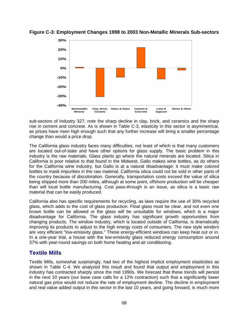
68

Figure C-3: Employment Changes 1998 to 2003 Non-Metallic Minerals Sub-sectors

-40%

-30%

-20%

-10%

0%

10%

20%

30%

NonmetallicMineral

Clay, Brick,Ceramic

Glass & Glass Cement &Concrete

Lime &Gypsum

Stone & Other

sub-sectors of Industry 327; note the sharp decline in clay, brick, and ceramics and the sharp rise in cement and concrete. As is shown in Table C-3, elasticity in this sector is asymmetrical, as prices have risen high enough such that any further increase will bring a smaller percentage change than would a price drop.

The California glass industry faces many difficulties, not least of which is that many customers are located out-of-state and have other options for glass supply. The basic problem in this industry is the raw materials. Glass plants go where the natural minerals are located. Silica in California is poor relative to that found in the Midwest. Gallo makes wine bottles, as do others for the California wine industry, but Gallo is at a natural disadvantage: it must make colored bottles to mask impurities in the raw material. California silica could not be sold in other parts of the country because of discoloration. Generally, transportation costs exceed the value of silica being shipped more than 200 miles, although at some point, offshore production will be cheaper than will local bottle manufacturing. Cost pass-through is an issue, as silica is a basic raw material that can be easily produced.

California also has specific requirements for recycling, as laws require the use of 30% recycled glass, which adds to the cost of glass production. Float glass must be clear, and not even one brown bottle can be allowed or the glass will be unsuitable for windows, which is a major disadvantage for California. The glass industry has significant growth opportunities from changing products. The window industry, which is located outside of California, is dramatically improving its products to adjust to the high energy costs of consumers. The new style winders are very efficient "low-emisivity glass." These energy-efficient windows can keep heat out or in. In a one-year trial, a house with the low-emisivity glass reduced energy consumption around 37% with year-round savings on both home heating and air conditioning.

Textile Mills Textile Mills, somewhat surprisingly, had two of the highest implicit employment elasticities as shown in Table C-4. We analyzed this result and found that output and employment in this industry has contracted sharply since the mid 1990s. We forecast that these trends will persist in the next 10 years (our base case calls for a 12% contraction) such that a significantly lower natural gas price would not reduce the rate of employment decline. The decline in employment and real value added output in this sector in the last 10 years, and going forward, is much more

69

the result of factors other than the price of natural gas such as the Northern American Free Trade Agreement (NAFTA), the rise of China, and the relocation textile mills to low-cost locations outside the United States. Our Low-price scenario forecasts an additional employment drop of 10% by 2016.

Table C-4: 2016 Impacts in Industry 313 - Textile Mills*

Change from Low-price to Middle-price Scenario Change from Low-price to High-price Scenario

Employment Employment

Level Percent Elasticity Level Percent Elasticity

-310 -2.4 -0.112 -500 -3.8 -0.051

* Includes Fiber, Yarn & Thread; Fabric Mills; and Textile & Fabric Mills

Transportation Equipment Fifteen years ago, California was home to 31% of all Aerospace & Aircraft Product & Parts jobs in the nation; today that ratio has fallen to one in five as California lost jobs in this sector to a far greater extent then did the rest of the nation. Figure C-4 shows how the level of employment in the California transportation equipment sector has steadily declined in the last 15 years. Table C-5 presents the employment impacts in this sector in 2016.

Table C-5: 2016 Impacts in Industry 336 - Transportation Equipment*

Change from Low-price to Middle-price Scenario Change from Low-price to High-price Scenario

Employment Employment

Level Percent Elasticity Level Percent Elasticity

-2,440 -1.9 -0.087 -4,540 -3.5 -0.047

• Includes Motor Vehicle; Motor Vehicle Body & Trailer; Motor Vehicle Parts; Aerospace & Aircraft Product & Parts; Railroad Rolling Manufacture; Ship & Boat Building; and Other.

The decline in federal defense spending in the early 1990s had a very significant impact on the economy of Southern California, as housing prices in the state fell for six years in a row. In Los Angeles, housing prices did not return to 1990 levels until 2000. In 1990 there were a total of 214,000 jobs in California’s aerospace products and parts manufacturing sub-sector, or 77.7% of total transportation equipment employment. As of November 2005, employment in the aerospace sub-sector had declined to only 76,000 jobs and 57% of total transportation equipment employment; however, even with the decline in aerospace employment, this sub-sector still dominates transportation equipment employment within California, especially when compared with the rest of the nation, where only 22% of all transportation equipment jobs are located in the aerospace sub-sector (as is shown in Figure C-5).

70

Figure C-4: Employment Trends in the Transportation Equipment Sector (Employment in Thousands)

Transportation Equipment

100

150

200

250

300

90 92 94 96 98 00 02 04

Figure C-5: 2003 Employment Shares Transportation Equipment Sub-sectors (Employment in Thousands)

0%

20%

40%

60%

Vehicles & Parts Aerospace Miscellanous

CA

Rest of US

Electrical Equipment and Appliances Employment in household appliance manufacturing in the state declined by half in the past 15 years, and employment in the entire electrical equipment and appliance sub-sector was down 24% in the same period. Table C-6 presents the impacts in this sector in 2016. As the table shows, above a certain level, rising natural gas prices would have a declining marginal effect on employment, as the implicit employment elasticity for the Middle- to Low-price scenario comparison is higher than that for the High- to Low-price scenario comparison. As is the case in other manufacturing sub-sectors, this suggests that, in response to rising natural gas prices, some of the employment savings have already occurred in this sector, so that future cost reductions must come from other measures, such as investing in more energy-efficient equipment and production processes.

71

Table C-6: 2016 Impacts in Industry 335 - Electrical Equipment & Appliance*

Change from Low-price to Middle-price Scenario Change from Low-price to High-price Scenario

Employment Employment

Level Percent Elasticity Level Percent Elasticity

-430 -1.4 -0.067 -930 -3.1 -0.042

* Includes Electric Lighting Equipment; Household Appliance; Electrical Equipment; and Other

Fabricated Metals The fabricated metal products industry is the third-largest manufacturing sub-sector in California based on employment, and is also one of the fastest-growing manufacturing industries in the state. Global Insight expects employment this industry to increase 12% in the next 10 years, and even under the High-price scenario considered in this study, we forecast employment will increase almost 9%. We found that employment in only four other manufacturing sectors, excluding textiles, is more sensitive to natural gas prices than is the fabricated metals sector. Table C-7 presents the impacts in 2016, while Figure C-6 shows employment levels since 1990.

Table C-7: 2016 Impacts in Industry 332 - Fabricated Metal Products*

Change from Low-price to Middle-price Scenario Change from Low-price to High-price Scenario

Employment Employment

Level Percent Elasticity Level Percent Elasticity

-2,430 -1.5 -0.069 -5,040 -3.1 -0.041

* Includes Forging & Stamping; Cutlery & Handtools; Architectural & Structural; Boiler, Tank & Container; Hardware; Spring & Wire; Machine Shops; Coating, Engraving & Heat Metals; and Other

Figure C-6: Employment Trends in Fabricated Metal Products

(Employment in Thousands)

Fabricated Metal Products

130

140

150

160

170

180

90 92 94 96 98 00 02 04

72

During the early 1990s, employment in this sector contracted significantly as is shown in Figure C-6; many of the firms servicing the defense sector were caught in the multi-year recession, but starting in the mid-1990s, the sector enjoyed a revival before the energy crisis hit it in the early part of this decade. We noted this occurrence in our state analysis at that time:

“The state energy crisis has also hurt the regional manufacturing sector. Two local manufacturers have left the area for less-expensive venues. Valentec-Wells, a metal stamping and plating company, closed its Costa Mesa plant in July and shifted operations to the lower-cost Midwest. Power outages made meeting customer demands difficult, and the company had to pay fines for using energy to fulfill orders, compounding the problem of already-high business and operating costs. Valentec’s 107 Costa Mesa employees were idled. Similarly, IPC communications, a printer and compact disc replication company, shifted some operations to Michigan and laid off 50 employees.”

Plastic and Rubber Products Employment in this sector is more sensitive to natural gas prices than are most of the other manufacturing sub-sectors as is shown in Table C-8. Rubber products use a higher share of natural gas as an input than does plastic, and like any industry dependent on natural gas prices, this sector has been adversely affected by rising prices. In 1990, the share of total manufacturing employment in this sector in California was similar to the national average, but in the past 15 years, plastics employment in California has remained constant, while the level of rubber employment has fallen 34%, and now the share of the state employment in plastics and rubber is about half that of the national share. In other words, with respect to rising natural gas prices in the plastic and rubber sector, the implicit employment elasticity is higher at the national level than in California, as the rest of the nation has a greater share of Sector 326 employment in rubber than in plastics.

Table C-8: 2016 Impacts in Industry 326 - Plastics & Rubber Products*

Change from Low-price to Middle-price Scenario Change from Low-price to High-price Scenario

Employment Employment

Level Percent Elasticity Level Percent Elasticity

-750 -1.4 -0.065 -1,590 -2.9 -0.039

• Includes Plastic Products (film, sheets, pipes, foam, bottle, & all other) and Rubber Products (tires, hoses, & all other)

Miscellaneous Manufacturing Other manufacturing is a diverse sub-sector comprised of a number of industries with very different characteristics, including their reliance on natural gas. This sub-sector is growing more rapidly than in any other manufacturing sector in California, with employment forecast to increase 20% in the next decade. Table C-9 presents the employment changes and implicit elasticities in the two scenarios in 2016.

73

Table C-9: 2016 Impacts in Industry 339 – Miscellaneous Manufacturing*

Change from Low-price to Middle-price Scenario Change from Low-price to High-price Scenario

Employment Employment

Level Percent Elasticity Level Percent Elasticity

-1,260 -1.1 -0.053 -3,070 -2.8 -0.037

* Includes Medical Equipment and Other (Jewelry, Silverware, Sporting goods, Toys, Marking devices)

Textile Mill Products This four-digit NAICS industry classification includes carpet and rug mills, curtain and linen mills, curtain and drapery mills, and other household textile products. Because of the high housing start rate in California in recent years, which has maintained demand for home furnishings, this sector has not experienced the same level of output and employment decline as has textile mills. As a result, the implicit employment elasticities in Table C-10 are lower than those in Table C-4 for textile mills.

Table C-10: 2106 Impacts in Industry 314 - Textile Product Mills*

Change from Low-price to Middle-price Scenario Change from Low-price to High-price Scenario

Employment Employment

Level Percent Elasticity Level Percent Elasticity

-260 -1.7 -0.077 -430 -2.8 -0.037

* Includes Textile Furnishings Mills and Other Textile Products Mills

Paper and Paper Products The sensitivity of employment in the paper manufacturing sub-sector to rising natural gas prices is similar to that in the entire manufacturing sub-sector as shown by the elasticities presented in Table C-11. The composition of the paper manufacturing sector in California is different from that in the rest of the nation, where high shares of paper manufacturing employment are found in the pulp mills, paper mills, newsprint mills, and paperboard mills sub-sectors. By contrast, California uses fewer workers in the first stage of paper manufacturing and specializes in the later stages when paper products are produced. The paper products sub-sector includes corrugated and solid-fiber box manufacturing, folding paperboard box manufacturing, fiber can, tube, drum, and similar products manufacturing, non-folding sanitary food container manufacturing, and setup paperboard box manufacturing. California mill employment fell 23% between 1998 and 2003, while paperboard container employment declined 11%, the smallest among all the paper manufacturing sub-sectors. The remaining sub-sectors are shrinking rapidly in California: paper bag manufacturing (-18%), stationary products (-26%), and other products (-33%). Several factors, including natural gas prices and the elimination of raw mill products in the state are hurting employment in the latter stages of processing.

74

Table C-11: 2016 Impacts in Industry 322 - Paper and Paper Product*

Change from Low-price to Middle-price Scenario Change from Low-price to High-price Scenario

Jobs Jobs

Level Percent Elasticity Level Percent Elasticity

-380 -1.4 -0.064 -680 -2.4 -0.033

* Includes Pulp, Paper & Paperboard Mills; Converted Paper Products which contains Paperboard Containers; Paper Bag and Coated and Treated Paper; Stationery Product; and Other Converted Paper product

Wood Products Employment growth in the wood products sub-sector has been the second-highest among all manufacturing sub-sectors in California in recent years. With the level of housing construction remaining high in California (195,300 housing starts during 2005) and high levels of non-residential construction, employment in wood products continues to expand to meet demand. For example, in the past 15 years, truss manufacturing and other related sectors have added 1,100 jobs in California. As a result of these demand drivers, employment in this sub-sector is less sensitive to rising natural gas prices than are most other manufacturing sub-sectors.

Furniture & Related Industries* * Includes Household & Institutional Furniture; Office Furniture & Fixtures; and Other

The entry of China into the furniture manufacturing sector has caused employment in California in this sector to drop sharply. California formerly employed 5,500 workers in the office furniture and fixtures sector, declines which have been partially offset by the growing household and institutional furniture sector. Employment and real output levels in the furniture sector are insensitive to rising natural gas prices.

Information* Looking outside the manufacturing sector, the Information sector is becoming an increasingly important part of the California economy, especially as it is a very productive sector with a high level of real output per employee. When comparing the High- and Low-price scenarios in 2016, as gas prices rise, the implicit employment elasticity is relatively high at -0.028, about twice the figure for total employment of -0.015 as shown in Table C-12. Recent employment trends in the Information sector are presented in Figure C-7.

Table C-12: Information*

Change from Low-price to Middle-price Scenario Change from Low-price to High-price Scenario

Employment Employment

Level Percent Elasticity Level Percent Elasticity

-7,260 -1.2 -0.064 -10,980 -1.8 -0.028

* Includes Publishing Industries (except Internet), Motion Picture and Sound Recording Industries, Broadcasting (except Internet), Telecommunications, Internet Service Providers, Web Search Portals, and Data Processing Services, Other Information Services

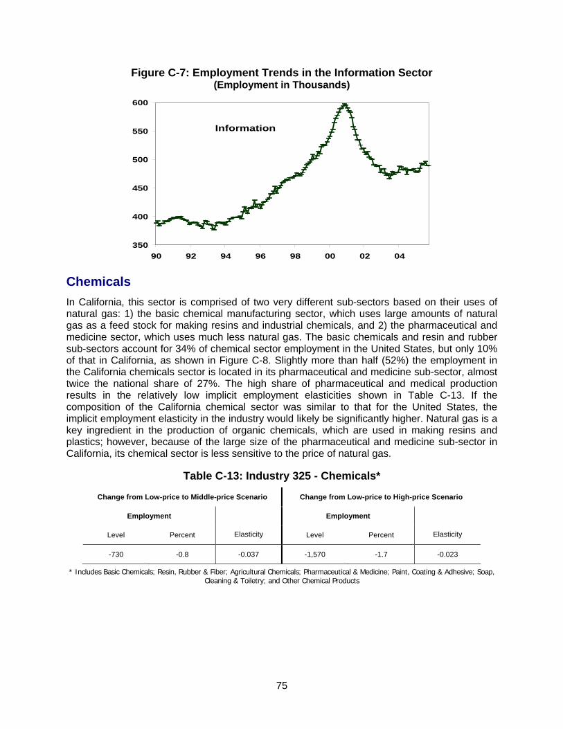
75

Figure C-7: Employment Trends in the Information Sector (Employment in Thousands)

Information

350

400

450

500

550

600

90 92 94 96 98 00 02 04

Chemicals In California, this sector is comprised of two very different sub-sectors based on their uses of natural gas: 1) the basic chemical manufacturing sector, which uses large amounts of natural gas as a feed stock for making resins and industrial chemicals, and 2) the pharmaceutical and medicine sector, which uses much less natural gas. The basic chemicals and resin and rubber sub-sectors account for 34% of chemical sector employment in the United States, but only 10% of that in California, as shown in Figure C-8. Slightly more than half (52%) the employment in the California chemicals sector is located in its pharmaceutical and medicine sub-sector, almost twice the national share of 27%. The high share of pharmaceutical and medical production results in the relatively low implicit employment elasticities shown in Table C-13. If the composition of the California chemical sector was similar to that for the United States, the implicit employment elasticity in the industry would likely be significantly higher. Natural gas is a key ingredient in the production of organic chemicals, which are used in making resins and plastics; however, because of the large size of the pharmaceutical and medicine sub-sector in California, its chemical sector is less sensitive to the price of natural gas.

Table C-13: Industry 325 - Chemicals*

Change from Low-price to Middle-price Scenario Change from Low-price to High-price Scenario

Employment Employment

Level Percent Elasticity Level Percent Elasticity

-730 -0.8 -0.037 -1,570 -1.7 -0.023

* Includes Basic Chemicals; Resin, Rubber & Fiber; Agricultural Chemicals; Pharmaceutical & Medicine; Paint, Coating & Adhesive; Soap, Cleaning & Toiletry; and Other Chemical Products

76

Figure C-8: 2003 Employment Shares in Chemical Manufacturing

0%

10%

20%

30%

40%

50%

60%

Basic Chemical Resin & Rubber Pharmaceutical Paint, Soap, Misc

CA

Rest of US

Petroleum and Coal Among all manufacturing sectors, we forecast that Petroleum and Coal sector will have the largest percentage employment decline (-26%) by 2016; higher or lower natural gas prices will only affect this decline at the margin, causing employment in this sector to fall within a narrow band (25–27%) based on price scenarios used in this study. The petroleum and coal sector is an industry in which productivity growth has reduced the number of jobs needed to produce the same level of output, so employment levels will continue to decline. California is home to 16% of all petroleum refining jobs in the United States. Table C-14 shows that employment levels in the petroleum and coal sector are relatively insensitive to increases in the price of natural gas, with higher natural prices initially increasing the production of petroleum as fuel substitution occurs, and as a result, generating a small rise in employment.

Table C-14: 2016 Impacts in Industry 324 - Petroleum and Coal*

Change from Low-price to Middle-price Scenario Change from Low-price to High-price Scenario

Employment Employment

Level Percent Elasticity Level Percent Elasticity

+110 +1.05 +0.049 -50 -0.4 -0.006

* Includes Petroleum Refineries; Asphalt Paving, Roofing & Related; and Other Petroleum & Coal Products

California is nearly self-sufficient in petroleum refining because of the very strict California Air Resources Conservation Board (CARB) standards for petroleum products. Although these standards increase the cost of gasoline and diesel fuels in California, they also limit competition from refiners in other locales, and, most importantly, provide a strong economic incentive to locate refining capacity within the state.

Petroleum refining is very energy-intensive and uses upwards of one-third of all industrial natural gas in California. Natural gas is used as a source of hydrogen and as a clean fuel for process heat, steam, and cogeneration. California has always been nearly self-sufficient in petroleum refining because of its geographic location and high local supply of crude oil. Petroleum refining uses extensive heat recovery and exchange as well as cogeneration of steam and power. California refineries are more energy-efficient than those in the rest of the

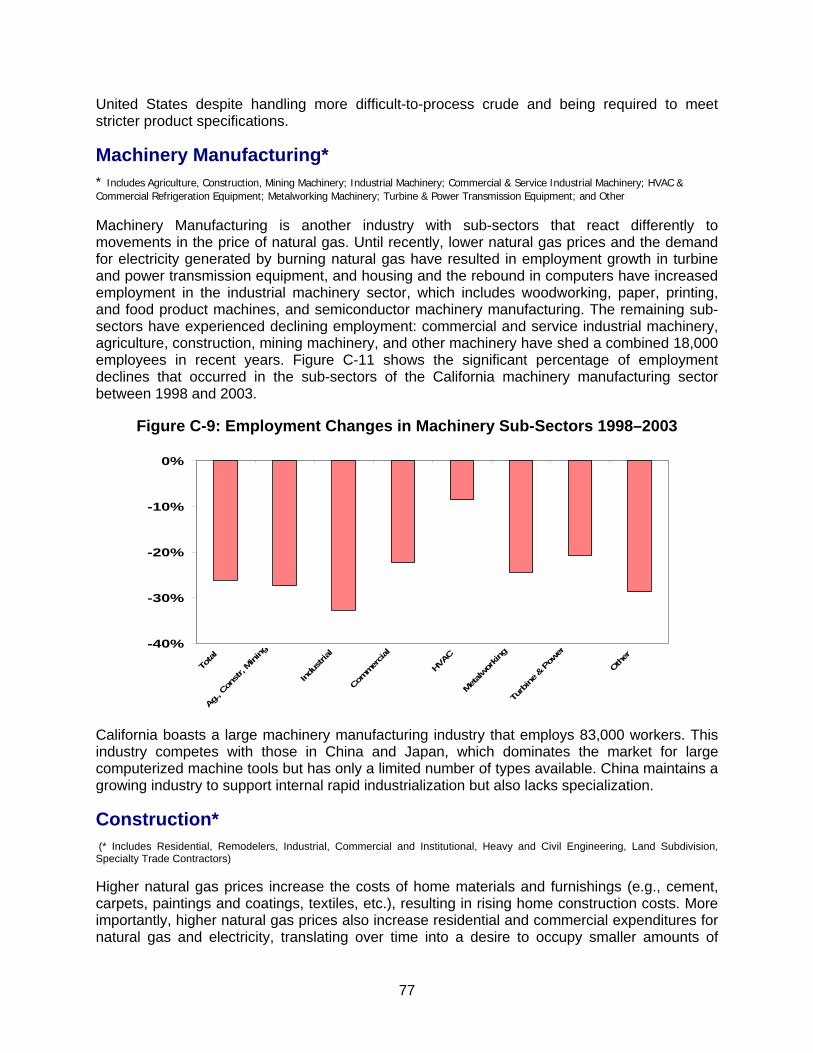
77

United States despite handling more difficult-to-process crude and being required to meet stricter product specifications.

Machinery Manufacturing* * Includes Agriculture, Construction, Mining Machinery; Industrial Machinery; Commercial & Service Industrial Machinery; HVAC & Commercial Refrigeration Equipment; Metalworking Machinery; Turbine & Power Transmission Equipment; and Other

Machinery Manufacturing is another industry with sub-sectors that react differently to movements in the price of natural gas. Until recently, lower natural gas prices and the demand for electricity generated by burning natural gas have resulted in employment growth in turbine and power transmission equipment, and housing and the rebound in computers have increased employment in the industrial machinery sector, which includes woodworking, paper, printing, and food product machines, and semiconductor machinery manufacturing. The remaining sub-sectors have experienced declining employment: commercial and service industrial machinery, agriculture, construction, mining machinery, and other machinery have shed a combined 18,000 employees in recent years. Figure C-11 shows the significant percentage of employment declines that occurred in the sub-sectors of the California machinery manufacturing sector between 1998 and 2003.

Figure C-9: Employment Changes in Machinery Sub-Sectors 1998–2003

-40%

-30%

-20%

-10%

0%

Total

Ag., C

onstr,

Mining

Indu

stria

l

Commer

cial

HVAC

Metalw

orkin

g

Turb

ine &

Pow

er

Other

California boasts a large machinery manufacturing industry that employs 83,000 workers. This industry competes with those in China and Japan, which dominates the market for large computerized machine tools but has only a limited number of types available. China maintains a growing industry to support internal rapid industrialization but also lacks specialization.

Construction* (* Includes Residential, Remodelers, Industrial, Commercial and Institutional, Heavy and Civil Engineering, Land Subdivision, Specialty Trade Contractors)

Higher natural gas prices increase the costs of home materials and furnishings (e.g., cement, carpets, paintings and coatings, textiles, etc.), resulting in rising home construction costs. More importantly, higher natural gas prices also increase residential and commercial expenditures for natural gas and electricity, translating over time into a desire to occupy smaller amounts of

78

office space and smaller homes. Even with these upward pressures on construction materials, and a demand for less floor area, Table C-15 shows that employment in the construction sector is relatively insensitive to rising natural gas prices. Figure C-10 shows the rapid increase in employment in the California construction sector that occurred throughout the 1990s, slowed during the 2001 recessions, and has resumed during the past few years.

Table C-15: 2016 Impacts in the Construction Sector

Change from Low-price to Middle-price Scenario Change from Low-price to High-price Scenario

Employment Employment

Level Percent Elasticity Level Percent Elasticity

-10,537 -0.9 -0.050 -16,100 -1.4 -0.022

Figure C-10: Employment Trends in the California Construction Sector (Employment in Thousands of Persons)

Construction

400

500

600

700

800

900

1000

90 92 94 96 98 00 02 04

Beverage & Tobacco Products* * Includes Soft Drink & Ice; Breweries; Wineries; Distillers. California does not have any Tobacco & Cigarette employment

California does not employ any workers in the tobacco industry, so the impact in this sector occur entirely within the beverage industries sub-sector. Due in large part to the huge increase in wine production, this sub-sector has experienced a 46% increase in employment in the last five years, as is shown in Figure C-11. The wine industry has become an increasingly important part of the California economy. As is shown in Figure C-12, only 6% of employment in the U.S. beverage sector was in wine sub-sector compared with more than 60% in California. Although it appears that California has low shares of employment in the soft drink and brewing sub-sectors, the total number of those employed as a percentage of the state population is consistent with the U.S. share. California has the same proportion of workers in soft drink bottling and water and ice manufacturing but a higher share in brewing, in part because microbrewers are a growing sector. By early 2003, wineries in California employed 19,000 workers and employed 75% of all workers at U.S. wineries. The wine industry enjoys a significant competitive advantage in California because of the climate and a critical mass that leads to efficiencies in

79

production, distribution, and marketing. More than 1,200 wineries are located in California, and generate retail sales of nearly $15 billion. The domestic wine industry, including California, is also benefiting from the decrease in the value of the U.S. dollar versus the euro, giving U.S. wines a competitive advantage over French and Italian wines. Energy use in the wine sub-sector is low, as is true of most of the beverage industry, and with rising demand, higher energy costs can be passed along to consumers. Even so, the wine industry has implemented a best-practices initiative to inform producers about ways to reduce energy consumption.

Figure C-11: Employment Trends in the Beverage Product Sub-Sector (Employment in Thousands)

Beverage Product Manufacturing (Thousands)

27

29

31

33

35

37

1991 1993 1995 1997 1999 2001 2003 2005

Figure C-12: 2003 Employment Shares in Beverage Manufacturing Sub-Sectors

0%

10%

20%

30%

40%

50%

60%

70%

W ineries B ottled S oft D rinks& Ice

B rew ers

C A

R est o f U S

Our study showed that when comparing the High- and Low-price scenarios, employment would decline by fewer than 500 jobs by 2106, with a low implicit employment elasticity of -0.018, which is insignificant in a 30,000-job sector.

80

Printing and Related Support Activities for Printing* * Includes Commercial Printing; Quick Printing; Digital Printing; Books; and Tradebinding & mounting

With elasticities of -0.033 and -0.017, employment sensitivity in this sector is near the state-wide averages, so that it would be relatively unaffected by changes in natural gas prices.

Industry 334 Computer & Electronic Products* * Includes Computer & Peripheral Equipment; Communications Equipment; Audio & Video; Semiconductor & Computer; Electronic Instruments; and Magnetic Media

The computer and electronic products sub-sector is a major part of the California manufacturing sector; in 2005 we estimate this it accounted for about 18.6% of California manufacturing employment but almost 25% of the value of output produced by the manufacturing sector. As is shown in Table C-16, under the High-price scenario in 2016, employment in this sector would be 3,670 fewer jobs than under the Low-price scenario, but with a below-average implicit employment elasticity of only -0.016. Recent experience has shown that rising costs force manufacturers of computer components to relocate production facilities elsewhere and to re-import the components back to the United States; however, if energy prices fall, not much additional domestic hiring is likely to occur. Figure C-13 shows that the level of employment in the California computer and electronic products sectors has been volatile but is trending steadily downward.

Table C-16: 2016 Impacts in the Computer and Electronic Products Sector

Change from Low-price to Middle-price Scenario Change from Low-price to High-price Scenario

Employment Employment

Level Percent Elasticity Level Percent Elasticity

-820 -0.3 -0.013 -3,670 -1.2 -0.016

Figure C-13: Employment Trends in the Computer & Electronic Products Sector (Employment in Thousands)

Computer & Electronic Products

300

325

350

375

400

425

450

475

90 92 94 96 98 00 02 04

81

Food Manufacturing* * Includes Animal Food; Grain & Oilseed; Sugar & Products; Fruit & Vegetable Preserving; Dairy Product; Animal Slaughtering & Processing; Seafood Production Preparation; Bakeries & Tortilla; and Other Food

Food manufacturing does not use as much natural gas or electricity as compared with other manufacturing sub-sectors; thus the effect of higher natural gas prices on employment is even less than that in the beverage products sub-sector. Figure C-14 shows a comparison of the 2005 employment shares in the food manufacturing sub-sectors between California and the United States; the sharpest differences are seen in the lower share in animal slaughtering seen in California, and its higher share in fruits and vegetables.

Figure C-14: 2005 Employment Shares of Food Manufacturing Sub-Sectors

0%

10%

20%

30%

40%

Animal

Food

Grain &

Oils

eed

Suga

r & Pro

ducts

Fruit &

Veg

etab

le

Dairy P

rodu

ct

Animal

Slau

ghter

Seafoo

d Pr

oduc

t

Bakeries

& Tor

tilla

Other Foo

d

California

Rest of US

The food manufacturing industries most affected by natural gas are sugar and sugar-related products, grain and oilseed, and bakeries and tortilla manufacturing, in that descending order. Of the three, only the bakery sector is an important part of the food manufacturing sector in California. The La Brea Bakery is a good example: it sells its product in 42 states and six foreign countries, but is still working off pre-purchased energy. Once the company finishes its pre-purchased lots, it will return to the market and will face much higher energy costs. Overall, food manufacturing has slightly increased within the state during the past 15 years, although activity at some high-profile manufacturers—like Frito Lay, which closed its Vistula plant—may not have filtered into the county data at the time of this report. Frito Lay decided the production required use of large fryers that use a lot of energy, making the plant unprofitable (at least in California).

Apparel* * Includes Apparel Knitting Mills; Cut & Sew Apparel; and Accessories & Other

The level of Chinese imports has become the most important determinant of the levels of employment and output in apparel manufacturing. As is shown below in Figure C-15, employment in California in this sector is down 55% since 1990. Unsurprisingly, of all the manufactured goods sectors, the apparel sector has seen the least change when natural gas prices move up and down. This sector has been steadily losing employment in California since the mid-1990s or shortly after the North American Free Trade Agreement (NAFTA) took effect.

82

Figure C-15: Employment Trends in the Apparel Sector (Employment in Thousands)

Apparel

75

100

125

150

90 92 94 96 98 00 02 04

Agriculture Our analysis showed that under the High-price scenario in 2016, employment would be about 3,800 fewer jobs than would exist in the Low-price scenario, with a very small implicit employment elasticity of -0.008. In other words, employment in agriculture is relatively unaffected by the rising price of natural gas, although clearly it affects sectors that supply agriculture inputs, such as the fertilizer sector.

Private, Services-Providing Sectors The private, services-providing sectors are comprised of the following NAICs super sectors: Trade, Transportation, and Utilities; Information, Financial Activities; Professional and Business Services; Education and Health Services; Leisure and Hospitality Services; and Other Services. The private, services-providing sectors currently account for about 67% of total employment (9.97 million jobs) in California; by 2016, we forecast its share of total employment will rise to just less than 69%. Excluding the Transportation and Utility sub-sectors, the primary impact of higher prices for natural gas and electricity is reflected in the costs of occupying office and store space. As is shown in Table C-17, the implicit employment elasticities for these sectors are virtually the same as for total employment, as was expected.

Table C-17: 2016 Impacts in the Private, Services-Providing Sectors *

Change from Low-price to Middle-price Scenario Change from Low-price to High-price Scenario

Employment Employment

Level Percent Elasticity Level Percent Elasticity

-67,425 -0.6 -0.031 -107,965 -0.9 -0.014

* Includes the following NAICs super-sectors: Trade, Transportation and Utilities; Information; Financial Activities; Professional and Business Services; Education & Health Services; Leisure & Hospitality Services; and Other Services.

Given the large size of the private, services-providing sectors, increases in the price of natural gas can leave large absolute impacts on employment despite low implicit employment

83

elasticities, as are shown in Table C-17. The employment impact in these sectors is highly asymmetrical, meaning that as natural gas prices increase, the marginal decline in employment decreases. In other words, employment is relatively unaffected by the upward movement in the price of natural gas as the cost of occupying floor space is a small share of the cost of production in these labor-intensive sectors.

Government The government sector consists of the federal, state, and local government sub-sectors, and currently accounts for about 16.2% of total employment in California. Employment and real output in the government sector is even less sensitive to the price of natural gas than in the private, services-providing sectors. Governments are major occupiers of office space, so they will also be affected by increases in natural gas and electricity prices; however, the government sector would not be affected as much by the lower levels of economic activity under the Middle- and High-price scenarios as are the private, services-providing sectors, not to mention the manufacturing sector. The lower levels of real GSP and real income under these two scenarios would not significantly reduce the demand for government services, many of which must be provided and will continue to be demanded, regardless of the level of economic activity. The one qualification to this finding is that government employment and real output could be affected if state revenues were to plummet sharply and suddenly amid a simultaneous increase in utility costs, as occurred during the utility crisis of 1991–92. Unsurprisingly, the implicit employment elasticities in the government sector are lower than those for the private, services-providing sectors, as is shown in Table C-18.

Table C-18: 2016 Impacts in the Government Sector *

Change from Low-price to Middle-price Scenario Change from Low-price to High-price Scenario

Employment Employment

Level Percent Elasticity Level Percent Elasticity

-5,230 -0.2 -0.011 -8,060 -0.3 -0.005

* Includes the federal, state and local government sub-sectors.