Working Paper Researchby Annelies Hoebeeck and Koen Inghelbrecht

September 2017 No 327

The impact of the mortgage interest and capital deduction scheme on

the Belgian mortgage market

NBB WORKING PAPER No. 327 - SEPTEMBER 2017

Editor Jan Smets, Governor of the National Bank of Belgium Statement of purpose:

The purpose of these working papers is to promote the circulation of research results (Research Series) and analytical studies (Documents Series) made within the National Bank of Belgium or presented by external economists in seminars, conferences and conventions organised by the Bank. The aim is therefore to provide a platform for discussion. The opinions expressed are strictly those of the authors and do not necessarily reflect the views of the National Bank of Belgium. Orders

For orders and information on subscriptions and reductions: National Bank of Belgium, Documentation - Publications service, boulevard de Berlaimont 14, 1000 Brussels Tel +32 2 221 20 33 - Fax +32 2 21 30 42 The Working Papers are available on the website of the Bank: http://www.nbb.be © National Bank of Belgium, Brussels All rights reserved. Reproduction for educational and non-commercial purposes is permitted provided that the source is acknowledged. ISSN: 1375-680X (print) ISSN: 1784-2476 (online)

NBB WORKING PAPER No. 327 – SEPTEMBER 2017

Abstract In 2005, mortgage interest, capital deductions and insurance premiums (MICPD) were assembled

into one single deduction package to further stimulate home ownership in Belgium. Former research

has shown that the MICPD did not raise the probability of becoming a home owner, due to its

capitalisation into higher house prices. The objective of this paper is to investigate how the

transmission of the capitalisation takes place. The analysis is based on data extracted from the

Household Finance and Consumption Survey. The mortgage amount, the mortgage maturity, the

interest rate and the house price are estimated simultaneously using a 3-SLS approach. The results

suggest that the mortgage deduction does not result in more affordable housing by shortening the

mortgage maturity. Most likely, the mortgage deduction results in larger amounts being borrowed,

which in turn may indirectly push up house prices, the mortgage maturity and the interest rate as

well. Although our estimation sample is rather small, these results suggest that the MICPD might be

more beneficial for sellers and mortgage-granting institutions than for home owners.

JEL classification: G21, H24, H31

Key words: Mortgages, tax policy, house prices, mortgage interest deduction, household borrowing

Authors: Corresponding author: Annelies Hoebeeck, Department Public Governance, Management and

Finance, Department Financial Economics, Ghent University - e-mail: Annelies.Hoebeeck@UGent.be. Koen Inghelbrecht, Department Financial Economics, Ghent University - e-mail: Koen.Inghelbrecht@UGent.be. This paper uses data from the first wave of the Eurosystem’s Household Finance and Consumption Survey. The results published and the related observations and analysis may not correspond to results or analysis of the data producers. The authors are grateful to Geert Langenus for his valuable comments concerning the research design and to Philip Du Caju for his clarification of the Household Finance and Consumption dataset. The authors greatly benefited from discussions with seminar participants at Ghent University and the National Bank of Belgium, and in particular with Freddy Heylen, Carine Smolders and Bart Cockx. The authors would like to thank M. Emiris and M.-D. Zachary for their extensive referee reports. Their constructive comments and suggestions helped us to improve the paper substantially. The views expressed in this paper are those of the authors and do not necessarily reflect the views of the National Bank of Belgium or any other institution to which the authors are affiliated.

NBB WORKING PAPER – No. 327 - SEPTEMBER 2017

TABLE OF CONTENTS

1 Introduction ............................................................................................................... 1 2 Introduction to the Belgian mortgage market ......................................................... 4 3. Theoretical considerations and international evidence ......................................... 8 3.1 Theoretical considerations ................................................................................... 8

3.2. International evidence .......................................................................................... 9

4 Dataset and model specification ........................................................................... 11 4.1 Data ................................................................................................................... 11

4.2 Selection bias .................................................................................................... 16

4.3. The empirical model ........................................................................................... 17

4.4. Indirect and direct effects ................................................................................... 20 5 Empirical results ..................................................................................................... 20 5.1 Parameter estimates and discussion.................................................................. 21

5.2. Direct versus indirect effects .............................................................................. 24

5.3. Robustness ........................................................................................................ 27

5.4. House size ......................................................................................................... 28

5.5. Type-2 mortgages .............................................................................................. 29

6 Conclusions and discussion ................................................................................. 31

References ...................................................................................................................... 34

Appendix ......................................................................................................................... 37

National Bank of Belgium - Working papers series .......................................................... 47

1. Introduction

In Belgium, like in many other countries, becoming a home owner gives access to sizeable tax benefits. The deductions in the personal income tax for mortgages were introduced in 1989. Mortgage interest payments qualified for a deduction, whereas capital amortisations were eligible for a tax credit. Mortgage protection insurance premiums could be eligible for a tax deduction or a tax credit, depending on certain conditions. As this system was very complicated, the tax benefits for interest payments, capital amortisations and mortgage insurance premiums were regrouped in a single deduction in 2005 (henceforth the MICPD). The purpose of the reform was to further increase the home ownership rate.

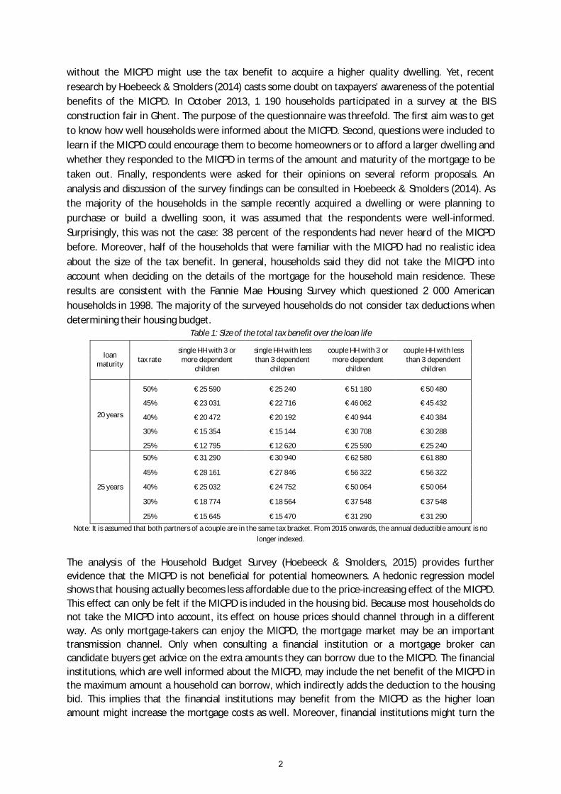
All mortgages of at least 10 years, which are taken out to construct or purchase the household main residence, are eligible for the MICPD if the borrower does not possess other dwellings. The MICPD can be enjoyed throughout the whole loan term. The main differences from the previous systems are that both mortgage-takers can enjoy the MICPD in all couple households1 and the maximum deductible amount no longer depends on the borrowed amount. The size of the net benefit depends on the tax bracket, which means that higher-income households get a larger tax benefit. The maximum deduction, which is indexed annually, amounted to 2 280 euros in the income year 2014. During the first decade of the loan maturity, a mark-up of 760 euros is allocated. If the household counts three or more children, the deduction is further increased by 80 euros. Table 1 shows the total net tax benefit a single household or a couple household can acquire over the life of a 20-year or a 25-year fixed-rate loan. Two remarks can be made. First, the size of the net benefit is quite considerable. Second, the household’s marital status and its tax bracket can lead to strongly varying tax benefits.

As far as we know, Belgium is the only country with a combined deduction for interest costs and capital2. Contrary to most mortgage interest deduction (MID) systems3, having diminishing tax benefits over time, here the size of the deductions depends on the monthly repayment of a fixed amount over the lifetime of the loan4. As a fixed deduction facilitates the calculation of the net benefit, rational and fully informed agents are expected to take this into account in their housing decision. Households might benefit from the MICPD in three ways: it could stimulate homeownership, affordability and the quality of the household’s main residence. First, credit-constrained households might qualify for a mortgage now, while they did not without the MICPD. Second, non-constrained households might use the MICPD to increase their monthly amortisation. A higher monthly amortisation ensures a faster repayment of the loan and consequently lowers interest rates. This would make housing more affordable. Third, households who can afford a home 1 In the previous system, only married mortgage-takers could enjoy a double benefit. 2 Spain and Portugal respectively had a tax credit for both interest cost and capital repayments from 1999 until 2012 and from 1998 until 2012. In Austria, acquisition and construction costs could be deducted together with other special expenses (Sonderausgaben) like pension fund premiums, insurance premiums and donations. From 1980 onwards, interest costs could be included as well. However, no deduction for mortgage amortisation can be claimed If the special expenses bucket is already filled up with other expenses. 3 The Statistical Appendix from the European Commission (2012) gives an overview of the different deduction systems. 4 This only applies to fixed-interest mortgages, which is generally the preferred type of home loan in Belgium. But it is likely that the deduction for adjustable-interest mortgages is relatively stable over the loan life as well. First, for most mortgages, the yearly amortisation largely exceeds the maximum deduction. Only a cut in the mortgage rate could lower the deduction. Over long periods of time, mortgage rates generally tend to rise. Moreover, the share of the capital amortisations in the total amortisation will increase when the pay-off period shrinks, which counters the declining mortgage rates.

1

without the MICPD might use the tax benefit to acquire a higher quality dwelling. Yet, recent research by Hoebeeck & Smolders (2014) casts some doubt on taxpayers’ awareness of the potential benefits of the MICPD. In October 2013, 1 190 households participated in a survey at the BIS construction fair in Ghent. The purpose of the questionnaire was threefold. The first aim was to get to know how well households were informed about the MICPD. Second, questions were included to learn if the MICPD could encourage them to become homeowners or to afford a larger dwelling and whether they responded to the MICPD in terms of the amount and maturity of the mortgage to be taken out. Finally, respondents were asked for their opinions on several reform proposals. An analysis and discussion of the survey findings can be consulted in Hoebeeck & Smolders (2014). As the majority of the households in the sample recently acquired a dwelling or were planning to purchase or build a dwelling soon, it was assumed that the respondents were well-informed. Surprisingly, this was not the case: 38 percent of the respondents had never heard of the MICPD before. Moreover, half of the households that were familiar with the MICPD had no realistic idea about the size of the tax benefit. In general, households said they did not take the MICPD into account when deciding on the details of the mortgage for the household main residence. These results are consistent with the Fannie Mae Housing Survey which questioned 2 000 American households in 1998. The majority of the surveyed households do not consider tax deductions when determining their housing budget.

Table 1: Size of the total tax benefit over the loan life

loan maturity tax rate

single HH with 3 or more dependent

children

single HH with less than 3 dependent

children

couple HH with 3 or more dependent

children

couple HH with less than 3 dependent

children

20 years

50% € 25 590 € 25 240 € 51 180 € 50 480

45% € 23 031 € 22 716 € 46 062 € 45 432

40% € 20 472 € 20 192 € 40 944 € 40 384

30% € 15 354 € 15 144 € 30 708 € 30 288

25% € 12 795 € 12 620 € 25 590 € 25 240

25 years

50% € 31 290 € 30 940 € 62 580 € 61 880

45% € 28 161 € 27 846 € 56 322 € 56 322

40% € 25 032 € 24 752 € 50 064 € 50 064

30% € 18 774 € 18 564 € 37 548 € 37 548

25% € 15 645 € 15 470 € 31 290 € 31 290

Note: It is assumed that both partners of a couple are in the same tax bracket. From 2015 onwards, the annual deductible amount is no longer indexed.

The analysis of the Household Budget Survey (Hoebeeck & Smolders, 2015) provides further evidence that the MICPD is not beneficial for potential homeowners. A hedonic regression model shows that housing actually becomes less affordable due to the price-increasing effect of the MICPD. This effect can only be felt if the MICPD is included in the housing bid. Because most households do not take the MICPD into account, its effect on house prices should channel through in a different way. As only mortgage-takers can enjoy the MICPD, the mortgage market may be an important transmission channel. Only when consulting a financial institution or a mortgage broker can candidate buyers get advice on the extra amounts they can borrow due to the MICPD. The financial institutions, which are well informed about the MICPD, may include the net benefit of the MICPD in the maximum amount a household can borrow, which indirectly adds the deduction to the housing bid. This implies that the financial institutions may benefit from the MICPD as the higher loan amount might increase the mortgage costs as well. Moreover, financial institutions might turn the

2

MICPD to their advantage by incorporating it in the mortgage rate or by encouraging borrowers to extend the mortgage maturity, which would enable them to enjoy the MICPD benefits for a longer period. However, it is unlikely that this extra tax benefit would offset the higher interest costs originating from a longer maturity.

This paper investigates whether the mortgage market is actually an important transmission channel for the MICPD to feed into higher house prices. The Belgian sample of the Household Finance and Consumption Survey (HFCS) will be used to disclose the transmission channel. First, the direct impact of the maximum annual net tax benefit from the MICPD on the mortgage characteristics of Belgian households is estimated simultaneously with its impact on house prices. More specifically, we will examine whether the tax benefit leads to larger mortgages of longer duration with higher interest rates, rather than to more affordable mortgages. Second, the indirect effects of the tax benefit on the household’s mortgage characteristics and house price will be calculated, as we are interested in the total effect of the tax benefit. In the third part of the analysis, we explore whether the changed borrowing characteristics affect the quality of household residences. As the HFCS dataset only contains details on the size of the dwelling, we estimate if the tax benefit has induced households to buy larger dwellings. Last, we examine whether the tax benefit affected mortgages granted after the purchase of the house differently than purchase mortgages.

Although our estimation sample is small, the results suggest that the maximum annual net benefit of the MICPD pushes up the house price indirectly through its direct effect on the amount borrowed. We find that an increase in the maximum annual net benefit of €100 would increase the borrowed amount by 2.5% and house prices indirectly by 1.5%. As the maximum annual net benefit varies between €915 and 2 975 in our sample, the MICPD may increase the mortgage amount considerably. No direct effect of the tax benefit is observed on the mortgage maturity, the interest rate or the house price. The indirect effects on the mortgage maturity and the mortgage rate are rather small, except for the highest tax benefits. In these cases, the mortgage maturity may indirectly increase by more than a year and the mortgage rate by 0.5 percentage points, which can have a significant effect on the total interest costs. The results of the house size regressions suggest that the extra money borrowed on the mortgage is not used to acquire a better quality dwelling, unless the mortgage is taken out for construction or renovation work. But it is very likely that the MICPD makes most housing less affordable. Furthermore, the higher mortgage may increase the interest costs and the notary and credit insurance fees. It seems that sellers and financial institutions will more likely benefit from the MICPD subsidy than homeowners will. For renovation or expansion mortgages, the MICPD might be more beneficial for he households. The extra amount borrowed might be used for a higher quality renovation or expansion project.

We contribute to the literature by investigating the impact of the MICPD on the Belgian mortgage market using microeconomic survey data. The Belgian case is of particular interest, as the maximum deduction remains the same during the first ten years of the loan. Although the effects of MID systems on home ownership have been extensively studied, evidence of their impact on the mortgage market is rather limited. This study could offer some important insight into the role of the mortgage market as a transition channel for tax benefits to feed into house prices. By disclosing the transmission channel, the paper seeks to raise the awareness of policy-makers on the possible side effects of a given tax benefit. Although their intentions might be good, it is important that government leaders consider all the repercussions these benefits might have for other markets. Next, this paper models the mortgage maturity, the mortgage amount, the interest rate and house prices simultaneously. As far as we know, no other studies have investigated the impact of a tax subsidy on these four household decision variables in one model. Finally, we estimate the impact of

3

the MICPD at the households’ point of decision, whereas most studies examine the effect of a tax benefit on the number (e.g. Bover et al., 2014; Jappelli & Pistaferri, 2007) and the amount of outstanding loans (e.g. Follain & Dunsky, 1997; Follain & Melamed, 1998; Jappelli & Pistaferri, 2007; Ling & McGill, 1998).

The remainder of the paper is structured as follows. Section 2 introduces the Belgian mortgage market. Section 3 gives some theoretical considerations and discusses the international evidence on the effect of tax benefits on mortgage characteristics. Section 4 describes the Belgian sample of the Household Finance and Consumption Survey and the construction of the variables. The same section also discusses the empirical model and some methodological issues and it explains how to calculate the direct and indirect effects of the MICPD. Section 5 reports the empirical results and some robustness checks. This section also presents a simple model to test whether the MICPD enables households to buy larger houses and an estimation of the MICDP effect on the mortgages taken out after the acquisition year. The last section concludes.

2. Introduction to the Belgian mortgage market

Chart 1 shows the financial liabilities of Belgian households over the last 15 years. From 1998 until 2001, total household debt (as percentage of GDP) remained relatively stable, whereas it doubled in the period afterwards. Mortgages have always constituted the main debt category and its share is still rising. The outstanding mortgage debt increased from 58 938 million in 1998, covering 64% of the total household debt, to 181 778 million in 2013, constituting 77% of the total household debt.

Chart 1: Financial liabilities of households (amount outstanding in % of GDP)

Source: NBB Stat, Online Database (Other financial statistics), 2015.

Chart 2 shows changes over time in the different purposes of contracting a mortgage. The average mortgage rate is also displayed. The number of new mortgages increased for all mortgage types in 2005. Based on this graph, it is hard to say whether this increase is only caused by falling interest rates or whether the MICPD inflated the size of the mortgage as well. Chart 2 also reveals that mortgage demand did not encounter any lasting crisis effect. Mortgage lending for purchasing or constructing a home declined slightly in 2008 and 2009, but demand soon recovered thanks to several anti-crisis measures. On the one hand, the VAT on new-builds was reduced from 21% to 6%, which boosted demand for construction mortgages. On the other hand, the beneficial tax treatment

0%

10%

20%

30%

40%

50%

60%

70%

1998 1999 2000 2001 2002 2003 2004 2005 2006 2007 2008 2009 2010 2011 2012 2013

Loans 1 year Mortgages Consumer credit

Other loans> 1 year Commercial loans

4

of “green loans” between 2009 and 2011 promoted the demand for renovation mortgages. These mortgages for energy-saving investment qualified for an interest rebate of 1.5% points and a 40% tax reduction. After the abolition of the green loan measure, the number of renovation mortgages fell back to its pre-reform level. The different peaks in the refinancing loans coincide with falling nominal mortgage rates.

Chart 2: Trend in the number of new mortgages according to the purpose of the loan (in 1000; on right axis) and change in the mortgage rate (in %; on left axis)

Source: NBB Stat, Online database (Other financial statistics), 2015 & semi-fixed mortgage rate CGER/Fortis Bank/BNP Paribas Fortis

Bank, 2015.

Chart 3 plots the transactions on the primary and the secondary real estate market against the accompanying mortgage loans. We observe a clear MICPD effect on the secondary market. All transactions from 2005 onwards are financed with a mortgage5, whereas before the introduction of the MICPD, only 80% of transactions were funded with a mortgage. For new builds, the gap between the number of new dwellings and mortgages for construction only narrowed in 2009 and in 2010 due to the green loan measures. We can think of several reasons why the MICPD has not increased the number of mortgages on the primary market. First, new real estate is often built by construction firms which are not eligible for the MICPD. This would also explain the increasing gap from 2012 onwards as there is a growing trend towards buying a dwelling from property developers rather than building one’s own house with a private contractor. Second, new real estate is generally more expensive than buying an existing dwelling, which means that it is more affordable for richer households who do not need a mortgage. Moreover, these richer households have a higher probability of possessing other real estate and hence do not qualify for the MICPD.

5 Of course, there are households with multiple mortgages, but it does not change the fact that the gap between transactions and mortgages has narrowed remarkably since 2005.

012345678

050

100150200250300350400

purchase and renovation other purpose

construction purchase

renovation refinancing

semi-fixed interest rate semi-fixed-real interest rate

5

Chart 3: Construction of new dwellings and purchases of existing dwellings and their mortgages (in 1000)

Source: FPS Economy (Statistics, Economics, Construction & Industry), 2015 & NBB Stat, Online Database (Other financial statistics), 2015.

The average amount borrowed for each type of mortgage loan and the average dwelling price are displayed in chart 4. The average mortgage amount is calculated by dividing the total credit granted by the number of mortgages. Nowadays, home buyers borrow between 45% and 60% more than they did in 1998. The average amount borrowed on the primary market has risen by 36% over the last 15 years. However, since 2004 the mortgage amount has no longer kept up with real estate price rises. In its 2012 Financial Stability Review, the NBB describes three household groups that might be responsible for the lower average loan-to-value (LTV) ratio. First, there is a trend for young households to buy a provisional dwelling before buying a larger final home. After a few years when the first dwelling is sold, the capital gains on the sale can be used to lower the LTV of the new dwelling. Second, in 2004, a one-off tax amnesty measure for unreported income was adopted, which might have stimulated the reinvestment of this money in real estate. Last, households who can afford a house without a mortgage would nevertheless contract one to enjoy the tax benefit of the MICPD. As these households are only borrowing the minimum amount to optimise the tax benefit, their LTV ratios are rather low as well (NBB, 2012).

020406080

100120140

in 1

000

building permits for new homes

new mortgages loans for construction

sales of houses and appartments

mortgages for puchase or purchase and renovation of dwellings

6

Chart 4: Changes in amounts borrowed (base year= 2010)

Source: NBB Stat, Online Database (Other financial statistics), 2015 & FPS Economy (Statistics- Economics- Construction & Industry), 2015.

Finally, chart 5 shows that Belgian households generally prefer 20-year, fixed-interest-rate loans. Variable-interest-rate loans only predominated in 2004 and 2010, probably because of the large gap between the long-term and the short-term interest rate in those years. The average maturity of new mortgages went up from 16.5 years in 2005 to 18 years in 2010 (Central Individual Credit Register, 2010, p. 8; De Doncker, 2006, p. 8). Increasing interest costs, relaxation of lending standards and securitisation might partly explain the longer mortgage maturities, but the MICPD may have played a role in it as well. From 2011 onwards, the average loan maturity started to fall again due to a more stringent policy of granting mortgage loans (Centrale voor kredieten aan particulieren, 2011, 2012, 2014).

Chart 5: Share of fixed-rate mortgages (in %; left axis) and the spread between long-term and short-term interest rates (in %; right axis)

Source: Financial Stability Review NBB (2011, Chart 6 Mortgage market developments in Belgium ) & OECD Economic Outlook Statistics and

Projections (2015). Note: The long-term and short-term interest rates are based on Belgian government bonds.

0

50,000

100,000

150,000

200,000

250,000

purchase and renovation other purpose

construction purchase

renovation refinancing

average dwelling price

-0.25

0.25

0.75

1.25

1.75

2.25

2.75

3.25

0

10

20

30

40

50

60

70

80

90

100

fixed spread (right scale)

7

3. Theoretical considerations and International evidence

3.1 Theoretical considerations

The impact of the mortgage interest deduction (MID) on housing is typically modelled in user cost models. In the simplest one, where maintenance costs, depreciation and expected capital gains are ignored, the cost of owner-occupied housing depends on the house price, the interest on mortgage or equity financing and the marginal tax rate on interest income. Three possible effects of the MID can be deducted from this simple model. First, the MID can lower the cost of investing in housing in comparison with investing in other non-deductible assets. This might boost housing demand, as concluded by Laidler (1969), for example. Second, the MID may change the relative costs of owning versus renting which affects tenure choice. H.S. Rosen and Rosen (1980) and Green and Vandell (1999) used this user cost approach to explain the increase in home ownership in the US. Several authors investigated both effects simultaneously (e.g. Glaeser & Shapiro, 2002; H S Rosen, 1979, 1985). Third, households might favour mortgage financing over equity because of the MID. In Follain and Dunsky (1997) households determine the cheapest combination of equity and mortgage financing depending on the after tax mortgage rates and the cost of equity financing. In the situation of a similar pre-tax cost of equity finance and mortgage debt, households would optimally choose mortgage finance after the introduction of the MID.

However, unless there is perfect supply elasticity, the rising demand for housing and/or mortgages will (partly) result in higher house prices. Since the discussion between Adams (1916) and Seligman (1916) about the possible beneficiaries of property taxation, this effect has been known as capitalisation in the economics of taxation and real estate literature. Capitalisation is short for the adjustment in the capital value of a property (Jensen, 1937), which occurs because the expected income of the property changes. Imposing a property tax would result in a lower selling price of the taxed dwelling in comparison with a similar non-taxed dwelling as the lower expected income is capitalised in a lower price. Likewise, a tax exemption will raise the value of exempt properties in comparison with non-exempt properties, as the expected income of the potential owner will be higher. In case of the MID, the capitalisation is generally assumed to accrue to the original owners, to real estate companies or to construction firms (e.g. Bourassa & Grisby, 2000; Bourassa, Haurin, Hendershott, & Hoesli, 2013; Cho & Francis, 2011; Gale, Gruber, & Stephens-Davidowitz, 2007; Glaeser & Shapiro, 2002; Hanson, 2012b; Hilber & Turner, 2014). However, Hanson (2012a) points out that lenders can benefit from the MID as well. He doubts the assumption of an exogenous pre-tax mortgage rate and observes higher mortgage rates for MID eligible mortgages. He concludes that on average 9 to 17% of the MID benefit is accrued by the mortgage lenders. Likewise, we also want to test if the lenders capture a share of the MICDP benefits. Unlike in Hanson (2012a), we allow lenders to benefit through other mortgage characteristics than just through the mortgage rates. Two arguments explain this decision. First, Hanson’s evidence that the MID benefits are offset by higher mortgage rates might be biased, as the authors do not take into account the endogeneity of the mortgage amount. Second, by disregarding mortgage maturity, the authors assume that the MID’s impact on the mortgage rate is the same, regardless of the number of years the tax deduction can be enjoyed.

The fixed Belgian deduction is comparable to the tax relief on British endowment mortgages. Devereux and Lanot (2003) compared their additional tax relief with the tax relief on standard repayment mortgages in the UK. Endowment mortgages consist of two parts: an interest-only-mortgage and an endowment premium, which is invested by insurance companies. The additional tax

8

relief on endowment mortgages arises because its interest payment is fixed over the loan life, whereas standard repayment mortgages have declining interest payments. The imperfectly competitive insurance sector offsets the benefits of the MID by charging higher endowment premiums. Lenders are found to capture 77% of the additional tax relief for endowment mortgages. The dependent variable, the share of monthly income dedicated to mortgage repayments, does not make it possible to distinguish in which mortgage characteristics the benefits are captured by the lenders. In the next section, we will give a brief literature overview on the possible effect of interest deduction systems on mortgage characteristics.

A user-cost model for Belgium was estimated by van den Noord (2003), who modelled the cost of borrowing in 1999. However, he only took the regular interest deduction into account. The additional mortgage deduction6, which usually implied a larger benefit, was completely ignored. The cost of borrowing since 2005 is even harder to model as the share of the interest cost diminishes and the capital payment share increases over time. As both capital payments and interest costs are eligible for the MICPD, the MICPD not only affects the cost of borrowing but also the net borrowed amount. Modelling the user costs implies estimating calculating the monthly payment before and after taxes. As the monthly payment depends on the mortgage amount, the interest rate and the loan maturity, it seems more interesting to investigate which of these factors is affected by the tax benefit. Considering the effect of the tax benefit on the monthly payment only could be misleading, as this payment can remain unchanged while its underlying determinants change. Therefore, we will model the impact of the MICPD on the main mortgage characteristics instead of estimating a user-cost model.

3.2 International evidence

In the US housing literature, several papers explore the effect of tax deduction systems on household debt. Follain and Dunsky (1997) estimate the elasticity of mortgage amount with respect to a cut in the tax rate at which the mortgage interest is deductible. Depending on the period estimated, an elasticity of -1.5 to -3.5 is found. For higher-income households, the elasticity is about -4. Follain and Melamed (1998) calculate the effect of the mortgage deduction being scrapped altogether in the United States. They find that the aggregate demand for mortgage debt would be 41% lower. Ling and McGill (1998) estimate housing consumption and mortgage debt simultaneously to account for the endogeneity of the house price in the mortgage amount equation. However, they do not focus on the effect of the MID on house prices. Only a proxy for the tax rate at which households can deduct their mortgage interest is included in the mortgage debt equation. They confirm earlier results that lowering the tax rates or completely abolishing the MID reduces mortgage demand. Maki (2001) provides additional evidence for the effect of tax deductions on the mortgage market. Owing to data unavailability, the author examines the changing pattern of the interest paid over time instead of the outstanding debt. The 1986 Tax Reform Act phased out consumer debt deductibility over a 5-year period. A difference-in-differences analysis shows that the total interest paid on outstanding consumer debt decreased for high-income homeowners but not for high-income renters after the reform. Scrapping the tax deduction has induced high-income home owners to substitute their consumption credit for mortgage credit.

In the European housing literature, the evidence of an MID effect on the mortgage market is mixed. Jappelli and Pistaferri (2007) use a difference-in-differences analysis to investigate the impact of the 1992 Italian tax reform on the outstanding mortgage amount. Mortgage interest deductions were no

6 See the last but one paragraph in section 4.1

9

longer dependent on the marginal tax rates of the households after the reform. A flat tax rate was introduced which should have increased mortgage demand for households with lower marginal tax rates and reduced it for households with higher marginal tax rates. However, the results do not show a clear relationship between the change in the tax benefit and the size of the mortgage. The authors attribute the absence of any effect to borrowing constraints and the lack of financial literacy. The borrowers probably are not sufficiently aware of the consequences of the reform to change their mortgage demand. Applying the same methodology to a comparable reform, Saarima (2010) observes a positive impact of the Finnish MID on mortgage demand. The 1993 Finnish tax reform replaced the progressive tax deduction by a constant tax rate, as in the Italian case. As the outstanding mortgage amount is not available in the Finnish Income Distribution Survey, the size of the annual interest payments is used as a proxy. The reform caused interest payments to rise for those households with marginal tax rates below the constant tax deduction rate. Households with higher tax rates reduced their mortgage demand after the reform. Surprisingly, the authors did not include the interest rate as a control variable. The latter obviously affects the annual interest payments.

Bover et al. (2014) test for a sample of 11 European countries if the availability of a mortgage deduction system inflates the mortgage amount. Although they find a positive effect, it is not significant. Different reasons might explain this result. First, their country-dummy variable does not take into account the size or duration of the deductions, nor the share of households that can actually benefit from the deduction. Second, all but two countries in the sample have a tax deduction for mortgage interests, so it is possible that the MID dummy variable captures another fixed effect for these two countries, rather than estimating the true impact of the mortgage interest deduction. Finally, the model disregards house prices, which is the main determinant of the mortgage amount. Martins and Villanueva (2006) do find an effect of the Credito Bonificado programme on long-term household borrowing in Portugal. The programme, launched in 1986, offers an interest subsidy up to 44% for lower income households wanting to purchase a house. The subsidy reduces the monthly amortizations immediately as it was directly given to the lenders. From 1998 onwards, houses with a selling price above a certain ceiling are no longer eligible for the programme. The authors show that the original Credito Bonificado programme increased mortgage amount and that the amount is more concentrated around the house price ceiling after the reform. The authors stated that banks did not offset the subsidy by higher interest rates. However, they did not discuss the benefits lenders could enjoy by increasing the mortgage supply up to the subsidy limit.

None of the above studies estimates the effect of the tax deduction on the initial mortgage amount. The use of the initial mortgage amount would assure a more precise estimate of the tax deduction effect as it avoids that the dependent variable is influenced by early redemption, overdue repayments or refinancing. Moreover, the tax deduction can only affect the initial mortgage characteristics on the loan origination date. Hendershott, Pryce, and White (2003) do estimate the loan-to-value ratio at the start of the mortgage loan. They investigate the effect of a complete elimination of the MID relative to a fictional full deduction on about 117 000 UK loans between 1988 and 1998. As the MID was limited to loans up to £30 000, they estimate the change in the loan-to-value for households with loans above and below the £30 000 ceiling. The loan-to-value ratio declined with 19 to 34% for the credit- constrained households and with 40 to 78% for the unconstrained borrowers. The aggregate loan-to- value decline was about 30%. In later work, Hendershott and Pryce (2006) also take the borrowing constraints of households into account as they can only borrow up to the value of the financed home. Moreover, they allow the loan-to-value ratio to differ between age groups and between first-time owners and previous owners. Scrapping the full mortgage deduction causes mortgage demand to drop by 17% to 23%. This decrease is smaller than

10

in their previous study due to the inclusion of constrained borrowers who cannot reduce their loan amount. First-time home owners experienced a drop of 7 and 16 % for the age groups 25-34 and 45-54 years respectively. Previous home owners encountered a drop of 12 and 35% for the same age groups. Morrizumi (2000) investigates the impact of a tax exemption dummy on the Japanese mortgage demand at loan origination date but finds no robust effect. Raya and Kucel (2016) estimate the impact of the Spanish mortgage interest and capital deduction on mortgage demand and mortgage maturity in a simultaneous model. A 1% increase in the ratio of the present value of the total tax benefit over the loan life on the property price is found to raise mortgage demand by 1.6 %. No explanation was given for the simultaneous 2% drop in mortgage maturity.

Although these studies theoretically model mortgage demand, the empirical analyses make use of the mortgage amount7, which is also influenced by mortgage supply. None of the studies considered the possibility that lenders might attempt to benefit from the tax incentive as well. Lenders might inform borrowers about the larger amounts they can borrow due to the tax benefit. Larger mortgage amounts give rise to higher interest payments, which are beneficial to the lenders.

Other studies explicitly investigate the impact of the interest deduction on the mortgage maturity. Dhillon, Shilling, and Sirmans (1990) prove that a tax deduction is an important determinant of choosing between a 30-year loan and a 15-year loan in the United States. They test the impact of the tax benefit of the mortgage interest deduction by including the ratio of the tax benefit for 15-year loans on the tax benefit for 30-year loans. A 10% reduction in the interest tax disadvantage of the 15-year mortgage increases the probability of choosing a 15-year mortgage by 30%. Vruwink and Fisher (1995) investigate the net cash difference between a 30-year and a 15- year mortgage, which arises due to the lower monthly payments and the higher tax deduction of a 30-year loan. If the net cash difference is well invested, it is possible to obtain a higher return with a 30-year mortgage than paying off faster and starting to invest after the repayment of the loan. The higher the marginal tax rate, the greater the net cash difference will be, which should induce higher income households to take out longer loans. These findings are confirmed by Baek and Bilbeisi (2011) who use Monte Carlo simulations to decide between a short- and a long-term mortgage. The mortgage maturity studies only consider the demand side as well. However, as the mortgage maturity granted rather than that demanded is analysed, the supply side should not be ignored. It is possible that lenders encourage their borrowers to opt for longer maturities, under the pretext of longer benefits, to get longer interest payments.

4. Dataset and model specification

4.1 Data

The Household Finance and Consumption Survey (HFCS) will be used to test our hypotheses. The HFCS dataset is interesting for our analysis as it collects an extensive range of information about a household’s borrowing behavior. The first wave of the HFCS collected household-level data on the finances and consumption of 2 327 Belgian households in 2010. This sample is chosen to be representative at the country level (ECB, 2013). Stratified sampling is used to select the households, with region and average income by neighbourhood of residence as stratification variables. The mortgage-related variables need to be representative as well to permit inference for the Belgian mortgage market. Appendix 1 compares some mortgage statistics from the HFCS sample with the mortgage market characteristics we discussed in section 2. As Appendix 1 shows that the mortgage

7 Except for Ling and McGill (1998), who estimate the desired mortgage amount with a latent variable approach.

11

characteristics in the HFCS sample do not differ drastically from Belgian mortgage market characteristics, the HFCS dataset can be used to extend the conclusions of the empirical analysis to the Belgian mortgage market.

Three types of loan are reported in the HFCS: the mortgage loan for the main residence, other mortgage loans and non-collateralised loans.8 We will only consider the first type, as it is the only one that can qualify for the MICPD. The households receive detailed questions about the two largest outstanding loans of each type. Next to the purpose of the loan, they provide information on the year the loan was taken out or the last time it was refinanced, the initial amount borrowed, the maturity of the loan and its interest rate. 74 % of the households surveyed own all or part of their residence and 38% of this group have at least one outstanding mortgage loan for the household’s main residence (HMR). All refinanced mortgages are removed from the sample as only the original mortgage makes it possible to calculate the tax benefit of the MICPD over the loan maturity. Mortgages taken out for other purposes than the acquisition or the renovation of the HMR are dropped from the sample. Two mortgages, which are both eligible for the MICPD9 but are taken out by the same household, are deleted from the sample as well. It is impossible to estimate the impact of the MICPD on the total borrowed amount or the maturity of the loans, as we cannot just aggregate both mortgages. Next, observations with missing values for the crucial variables, like the origination year of the mortgage, are eliminated. In order to prevent biased results, observations with house prices outside the [€ 40 000 to € 650 000] interval are dropped from the sample. Initial mortgages which do not exceed € 10 000 or exceed € 550 000 are deleted as well. 10 The final sample consists of 414 mortgages that were taken out between 1981 and 2010. Two types of mortgage can be distinguished. The first type are mortgages granted to acquire the household’s main residence. These mortgages are taken out in or prior to the acquisition year. The second type of mortgages, which are taken out after the acquisition of the home, might have been contracted for renovation or remodelling purposes, buying co-owners out after an inheritance or a divorce, or for an expansion of the residence. As these mortgages can be eligible for the MICPD as well, we will investigate whether the MICPD affects them differently than the acquisition mortgages. The final sample consists of 346 mortgages of the first type and 68 mortgages of the second type.

8 Only a limited number of households have other mortgage loans besides the mortgage for their main residence. These mortgages are used to finance a holiday residence or real estate, rented out or used for business activities. About half of the HFCS sample has at least one non-collateralised loan. These loans are mainly used to finance a vehicle purchase or other large purchases. Although a mortgage seems a more appropriate choice, some households take out non-collateralised mortgages to finance housing-related costs. 9 Mostly two mortgages taken out in the same year. 10 We restrict house prices and borrowed amounts to a bound of the first quartile minus 3 times the interquartile range and the third quartile plus 3 times the interquartile range.

12

The dependent variables, mortgage amount (A), mortgage maturity (M), the mortgage rate (R) and house price (H), are all examined at the loan origination date. The mortgage amount is the logarithm of the initial amount borrowed when the loan was first granted. The consumer price index with base year 2010 is used to express the mortgage amount in real prices. Mortgage maturity is the number of years that were agreed for the length of the loan when the loan was granted. The house price is the household’s answer to the question how much its main residence was worth at the acquisition date. We assume that this amount equals the selling price of the house as the household agreed to acquire the house at this particular price.11 For mortgages taken out before or after the acquisition year, we adjust the house price to reflect the value in the mortgage year. To this end, the house price is assumed to have changed with the general movement in prices of the average Belgian dwelling. The house price variable is always expressed in logarithms and in 2010 prices.

The explanatory variables are defined in Appendix 2. The mortgage characteristics are all observed at the loan origination year, except for the interest rate for the adjustable-rate mortgages, which is the rate since the last fixation. Unfortunately, the HFCS does not contain sufficient information to calculate the initial adjustable mortgage rate. The real mortgage rate is calculated according to the Fisher equation. For some household characteristics, like its average age, number of children and employment status, it is trivial to retrace them back to the loan year. The household income requires more effort. We use the household’s permanent income as an explanatory variable instead of the household income at loan origination date, as the latter cannot be calculated. Moreover, using the permanent income has two advantages. First, the permanent household income is a better determinant of the house price (Goodman & Kawai, 1981; Page, 1964) and the mortgage characteristics (Dhillon et al., 1990) than the household income. Second, using the permanent income of the household avoids endogeneity, as it is less closely correlated with the household characteristics at the loan origination date. In order to estimate the permanent income, we use Goodman’s (1998) human capital model. This model considers the current income as a function of the permanent income and a transitional component. As the permanent income depends on the human capital characteristics and some demographics of the household, the fitted value of the current gross income on a household’s human capital characteristics proxies the permanent income of the household. The permanent income regression is shown in Appendix 3. The adjusted R² is 0.45 which is larger than the R² found by Raya and Garcia (2012), who use the same method for a larger sample.

The HFCS contains only two housing characteristics: the house size and the dwelling type (existing dwelling or new construction). The house size is provided in brackets, hence we assume that the house size has only varied between those brackets since the loan origination year. This assumption is not too strict, as none of the mortgage takers in our sample has taken out a second mortgage after the loan year to expand or renovate the dwelling. Moreover, it is unlikely that a household downsized.

11 We assumed the house price measure to be equal to the selling price exclusive of taxes. If a household did not believe the value of its dwelling was worth the selling price, it would not have paid that price. It is possible though that the household believes the main residence is worth more than what it has paid for it. However, there is no way of controlling for this possible overvaluation relative to the selling price. Moreover, we cannot be certain that the house price measure includes taxes. However, we can assume that all households, which are advised by the interviewers, answered the question in the same way. It is most likely that households who constructed their home report the house price with VAT included, whereas households who purchased a residence on the secondary market report house prices without registration tax.

13

The HFCS dataset is particularly interesting for our analysis as it contains both the loan origination year and the acquisition year of the household’s main residence. This enables us to determine for each household if the borrowers qualified for the MICPD at the start of the loan. All households who have taken out a mortgage loan since 2005 to purchase or renovate their main residence qualified for the MICPD if the mortgage had a maturity of at least ten years and the household did not own other properties prior to the start date of the loan. Out of the 346 mortgages in the sample, 112 are eligible for the MICPD. We will investigate the impact of the maximum annual net benefit of the MICPD. We prefer the net benefit, as the actual benefit of the MICPD is determined by the income tax rate. Moreover, we will use the annual benefit of the MICPD as it does not depend on the mortgage maturity. We also choose to use the maximum benefit instead of the effective benefit, as it does not depend on the mortgage amount or the mortgage rate. As the size of the net benefit depends on the tax bracket one is in, we need to know the taxable income of each household. The estimated gross permanent income is divided into three income categories in order to calculate the taxable share of each category. We assume that the share of each income category in the permanent income at the loan origination date is the same as its share in the survey year. The total permanent income consists of the sum of the permanent income from immovable property, the permanent earned income and the permanent income from movables.12 Social security contributions and fixed expenses are deducted from the permanent labour income to calculate the taxable earnings. The matrimonial coefficient is applied to the taxable earnings of married and legally co-habiting households. This means that a share of the labour income of the highest earner is allocated to his/her partner, if the partner gains less than 30% of the total earned household income. Income from movable assets is subject to a separate tax rate and thus is not taken into account to determine the tax bracket for the MICPD deduction. The gross property rent is added to the taxable earned income as it is subject to the same tax rate. If the taxable income exceeds the tax-free minimum13, the tax rate (t) for each taxpayer is determined according to table 2.14 For the sake of convenience, the tax rates for 2010 are used for all calculations. As there were no major changes in the tax system from 2005 to 2010, it is unlikely that this assumption will affect our conclusions. The tax rates did not change over the considered period, but in some years the tax brackets were adapted slightly to correct for inflation and rising income. Moreover, the lender who grants the mortgage cannot consider future tax changes.

Table 2: Tax rates

12 We disregard miscellaneous income as only eight households in our sample reported having received income from this category and we have no further information of the source of this income, which makes it impossible to calculate the taxable share. 13 The tax-free minimum is EUR 6 690 for taxpayers whose taxable income is lower than €23 900 and € 6 430 for taxpayers with a higher taxable income. The tax-free minimum rises for each dependent child and the increase is higher if the child is less than 3 years old. 14 Appendix 4 shows the number of households per tax rate for couple and single households.

Tax bracket (2010 prices) Tax rate (t) €0 - €7 900 25%

€7 900 - €11 240 30% €11 240 - €18 730 40% €18 730 - €34 330 45%

> €34 330 50%

14

The annual deductible amount (DA) is determined by the annual amortisation if it does not exceed the maximum deduction. In the first 10 years of the mortgage, the maximum deduction ( ) is increased by € 690 and an extra increase can be obtained for households with three or more children in the year following the acquisition year (C=1).

= min(2770 + 70 , ) (1)

= min(2080, ) (2)

As said before, we will only use the maximum deduction, as it is not determined by the dependent variables. Moreover, the deductible amount equals the maximum deduction for all but 21 mortgages in our sample. For each mortgage-taker, we calculate the maximum annual net tax benefit for the first 10 years of the mortgage ( ) and for the remaining amortisation period ( ). The maximum annual net tax benefit depends on the income tax rate t and the municipality tax rate . As the HFCS dataset does not contain location characteristics, we use the average municipality tax rate in 2010, which is 7.4%.15 The annual maximum net tax benefits are expressed in €100.

= (1 + ) /100 (3)

For eligible households, ranges from 9.15 to 29.75 and ranges from 6.70 to 22.43. The left-hand limit is the maximum annual net tax benefit of a couple household with three children, in which one household head does not pay income tax and the other one has a marginal tax rate of 30%. The right-hand limit is the maximum annual net tax benefit for a couple household without children, in which both household heads have a marginal tax rate of 50%. For non-eligible households, thus also for all the households who took out a mortgage prior to 2005, equals zero.

Ideally, we should also include the tax benefit systems prior to the MICPD in our estimation model. Unfortunately, the HFCS does not make it possible to calculate the tax benefit prior to 2005 due to the complexity of the system. Before 1989, there were two systems. From 1963 until 1986, the interest was deductible up to the real estate income. Capital amortisations for social dwellings where fully deductible, whereas the deduction was limited for normal dwellings. Large dwellings did not qualify for a deduction. In 1986, the deduction limit of new builds was extended and an additional interest deduction for new builds and renovation mortgages was introduced. From 1994 onwards, a tax credit replaced the capital deduction. The HFCS dataset does not enable the real estate income to be calculated for the start year of the mortgage. A different system for capital amortisations and for interest costs prevents the calculation of an annual tax benefit, as it will differ yearly. Construction or renovation mortgages qualified only for the additional interest deduction when the construction or renovation costs exceeded a certain limit. The eligibility for the additional mortgage deduction also depended on the age of the dwelling. Unfortunately, this kind of information is not available in the HFCS. Moreover, as capital amortisations were entitled to a tax credit, calculating a household’s marginal tax rate is not sufficient to calculate the net benefit, as the total taxes owed to the government are needed too. In section 4.3, we will explain how we deal with the unobserved tax benefits prior to 2005. The HFCS provides five different imputed values for missing values to reduce the uncertainty of the imputation. A detailed description of the imputation process can be consulted in the HFCS database

15 The municipality tax rate varied between 5.7 and 8.8% in 2010.

15

description file (European Central Bank, 2012). All analyses are performed for each imputation file. The results presented in this paper are combined results across the five imputations.16 4.2 Selection bias

As only outstanding mortgages are observed in the HFCS dataset, we have to cope with a selection bias problem. Chart 6 illustrates this problem clearly. Mortgages that were taken out in 1980 should had a maturity of at least 30 years to be observed in 2010; mortgages that started in 1990 need a maturity of at least 20 years to shown up in the dataset. We apply a two-stage Heckman procedure, as described in Woolridge (2009, Chapter 17 ), to solve the selection bias problem. In the first stage, a probit regression estimates the probability of being selected in our sample. Therefore, the sample is extended to unselected households. These are the households in the HFCS sample who became a homeowner between 1980 and 2010 but who no longer had an outstanding mortgage in 2010. As almost all owner-occupied dwellings are financed with a mortgage, it is a reasonable assumption that the unselected households once had a mortgage as well, but that it is already paid off in 2010. Appendix 5 shows the first-stage regression. We used two predictors to estimate the probability of being selected in the sample. A dummy variable for retirement of the homeowners negatively affects the selection probability, as retired homeowners are less likely to obtain a mortgage. Households who own a second property in the survey year are more likely to have repaid their mortgage for their first home. Following Woolridge’s advice, we added all the exogenous variables of the simultaneous equation model to the selection model as well. The acquisition year, the household age in the acquisition year, the house size and having a job in the financial sector also affect the participation probability. Using a cut-off value of 0.5, the selection model correctly assigns 81% of the households to the right group. Hence, we can use the estimated probability of being selected in the model to calculate the inverse Mills ratio ( ). In the second step, this ratio is added to the simultaneous

equation model.

Chart 6 Selection bias

Data source: HFCS (2013)

16 The estimated coefficients are averaged across the five imputation files. Standard errors and R² are calculated according to Rubin (1987) and Harel (2009).

16

4.3 The empirical model

In order to test whether the MICPD is capitalised through the mortgage market instead of directly through the housing bid, we will investigate in one model how the maximum annual net tax benefit affects the mortgage maturity (M), the mortgage amount (A), the mortgage rate (R) and the house price (H).17

As the households decide simultaneously on the house price and the mortgage characteristics, there is some contemporaneous correlation between the error terms of the four equations. Equation by equation estimation is consistent but not efficient as the error terms of each loan will be correlated across the different equations (Gujarati, 2004). A seemingly unrelated regression will take this simultaneity bias into account. The model can be represented as:

= + + + + + + (4)

= + + + + + + (5)

= + + + + + + (6)

= + + + + + + (7)

where is a vector of exogenous variables for household i used in equation , is the maximum annual net tax benefit of the MICPD for the first 10 years ( = 1) or for the remaining mortgage maturity ( =2), are the error terms which are correlated across the four equations. The exogenous

variables include mortgage characteristics, household characteristics, dwelling characteristics and some other variables, as explained in Appendix 2. The coefficients measure the impact of the maximum annual net tax benefit on respectively the mortgage maturity, the mortgage amount and the house price, which is the focus of our paper.

To ensure that each equation is identified, the order and rank conditions need to be fulfilled. The order condition states that the number of variables excluded from an equation must be equal to or greater than the number of endogenous variables in the model less one (Gujarati, 2004 , p. 748). In practice, this means that at least three variables in has to be restricted to zero in each equation. In the mortgage maturity equation, we set the variables interest on government bonds, mortgage purpose, second mortgage for HMR, two mortgage-takers, inheritance or gift, other property mortgage, nest leavers, new house and acquisition year to zero, as those variables only indirectly affect mortgage maturity through the mortgage amount, the mortgage rate or the house price. The interest on government bonds is the main determinant of the basis mortgage rate. Except through its effect on the mortgage rate, it does not affect mortgage maturity. The mortgage purpose may affect the mortgage maturity indirectly through several channels; however, there is no direct effect of the mortgage purpose on mortgage maturity. The mortgage purpose determines the required mortgage amount and it may affect the mortgage rate and the house price. Households who only borrow the renovation budget have more financial means and are thus more creditworthy. A possible lower mortgage rate might be the result. As the mortgage purpose indicates whether the house requires renovation work, it can also directly affect the house price. A second mortgage for the HMR 17 According to Haurin and Lee (1989), the length of stay has to be modelled simultaneously with the mortgage amount as well. Households decide how long they will stay in the house before they purchase it and before the mortgage is taken out. Although their arguments seem valid, our dataset does not make it possible to calculate the expected length of stay in the house.

17

obviously reduces the size of each mortgage. It may also push up the households’ risk premium and it indicates that the house is more expensive. As those factors increase the total monthly payment, the mortgage maturity might be extended indirectly as well. Two mortgage-takers have a higher permanent income and thus can afford a larger monthly payment and indirectly a shorter mortgage maturity. Two mortgage-takers may also indirectly affect maturity through a downward effect on the mortgage rate premium. An inheritance or gift prior to the acquisition year might induce households to buy a more expensive house and it may reduce mortgage demand, but it has no direct effect on mortgage maturity. Possessing a mortgage for a property that is not the HMR may reduce a household’s down payment, which indirectly extends mortgage maturity through a higher borrowed amount, but there are no direct effects. Households with nest leavers, children of 18 years or older, will experience a rise in disposable income in the near future when their children leave the house. This induces those households to borrow more now. Possibly, it also lowers the risk premium on the mortgage rate. However, the nest leavers variable does not directly affect the mortgage maturity, as a higher future income does not change the repayment period at the start of the loan. A new house only indirectly affects the mortgage market through the house price and possibly through a higher mortgage amount. As a new house also entails higher costs, like higher notary fees, the mortgage amount might be pushed up directly too. The continuing rise in house prices is captured by the acquisition year. There is no need to include this variable in the mortgage equations, as general changes in the mortgage market are already included in the amount of the mortgage and the interest rate on it.

In the mortgage amount equation, we exclude the variables interest on government bonds, variable mortgage rate, two mortgage takers, household age, financial sector, number of children, house size and acquisition year. Borrowing-constrained households are more likely to choose a floating-rate mortgage (Johnnson & Geng, 2014; Linneman & Wachter, 1989). An upward revision of the adjustable mortgage rate might hamper consumption smoothing of constrained borrowers less when they have longer maturities. A dummy for adjustable-rate mortgages is thus included in the mortgage maturity equation. Changing the mortgage amount does not smooth interest changes and thus we do not include the mortgage rate in the mortgage amount equation. Two mortgage-takers might be allowed to borrow more as they may have a lower mortgage rate and a higher permanent income. Those determinants are already included in the mortgage amount equation, so there is no need to include the two mortgage-takers variable as well. The household age in the acquisition year represents the expected life expectancy, which directly affect mortgage maturity. Household age also proxies a household’s life stage which determines the housing amount. However, age only indirectly affect the mortgage amount through its effect on the permanent income. Financial sector employees often get a variable wage depending on the number of mortgages, savings accounts, and on other financial products they sell. Therefore, their income is volatile, which makes them opt for longer maturity mortgages to lower the probability of default. The mortgage amount (both supply and demand) depends on the average wage, which is already captured by the permanent income. Mortgage supply does not depend on the number of children. Mortgage demand only indirectly depends on the number of children through an effect on the house price, the mortgage maturity and the mortgage rate. House size only indirect affects mortgage amount through the house price and possibly the mortgage maturity too.

In the mortgage rate equation, we exclude the variables inheritance or gift, other property mortgage, household age, new house, house size and acquisition year. A household’s mortgage rate is

18

determined by its credit risk and the standard mortgage rate. An inheritance or gift only indirectly affects the credit risk through a lower mortgage demand and a higher house price. Unlike a second mortgage for the HMR, a mortgage for another property does not affect the creditworthiness of the household as the other property guarantees the repayment of that mortgage. The household age might affect credit risk through permanent income and mortgage maturity. As those variables are already included in the mortgage rate equation and we cannot think of any other reason why the household age would affect the credit risk, we restrict it to zero. The house size and type only indirectly affects the credit risk through the house price and the mortgage rate.

In the house price equation, the coefficients on the variables interest on government bonds, variable mortgage rate, two mortgage-takers, other property mortgage, financial sector, tertiary education, number of children and nest leavers are restricted to zero. The interest on government bonds does not affect house prices differently than through the mortgage rate. Whether the mortgage is of fixed or variable rate does not affect house prices directly either. Two mortgage-takers may have higher house prices, as they have a higher permanent income, a higher mortgage amount and a lower mortgage rate than single mortgage-takers. A mortgage for property different from the HMR may only indirectly affect the house price through its effect on the mortgage amount. Similarly, the house price does not depend on the volatile income, but on the permanent income. The financial sector variable is thus restricted to zero in the house price equation. Households with tertiary education might end up with shorter mortgages than households who studied less, because the risk of becoming unemployed is lower and they may be more informed about the extra cost of longer loans. The future income prospects of those with tertiary education lowers the risk for the credit institutions, which may affect the amount lent and the mortgage rate. Moreover, more highly-educated households have a higher permanent income as well. As these variables are already controlled for in the house price equation, higher education can only affect house prices indirectly. The number of children is excluded from the house price equation as this variable only affects the house price through the required house size, which is already included. Nest leavers do not influence the house price either as they still live in the house for a couple of years.

The variable occurs in every equation in order to reveal the transmission of the capitalisation. The parameter will capture the variation in the maximum annual net tax benefit across the eligible mortgage takers. As the tax benefits prior to 2005 cannot be calculated, we add a dummy variable for the period since 2005 in each equation. This dummy controls for other factors that might have affected the mortgage market since 2005. It avoids events like the 2004 fiscal amnesty measure18 being captured by the tax benefit variable. The inverse Mills ratio is added to the mortgage maturity and the mortgage amount equation. We do not include the inverse Mills ratio in the mortgage rate equation and the house price equation as high correlations between this variable and respectively the interest on government bonds and the acquisition year cause multicollinearity. The rank condition will be tested after estimation. An equation is identified if the matrix from the coefficients of the variables excluded from that equation is of full rank (Gujarati, 2004, p 752).

18 As a permanent fiscal regularisation was introduced in 2006, the fiscal amnesty measure existed almost for the whole period since 2005. It might have affected the mortgage market and house prices as a large share of the repatriated money might have been invested in the housing market Baugnet, Butzen, Cheliout, Melyn and Wibaut (2011).

19

Seemingly unrelated regression would be biased as all four equations contain endogenous right-hand side variables. As three-stage least squares (3SLS) combine seemingly unrelated regression with two-stage least squares (2SLS), this is the preferred method for our analysis. Moreover, it is shown that the estimation of an equation with 3SLS is more efficient than 2SLS if the other equations are over-identified (Zellner & Theil, 1962), which is the case for all four equations. However, if one of the structural equations is misspecified, 2SLS is more robust as the incorrectly specified equations will not affect the other equations (Woolridge, 2010). For the latter reason, we will estimate a 2SLS regression as robustness test. The same instrumental variables, i.e. all the exogenous explanatory variables of the whole system, are used for all four equations. A Sargan test of over-identifying restrictions will be performed to test the exogeneity of our instruments. The fourth equation will be dropped for mortgages taken out after the acquisition year as the MICPD for these mortgages can no longer affect the acquisition value of the house.

4.4 Indirect and direct effects

The model estimation model contains feedback loops as the dependent variables are appearing on both the left-hand and the right-hand side of the equations. The right-hand-side variables can thus indirectly affect the left-hand-side variables as well. The estimated regression coefficients only represent the direct effect of explanatory variables, but as we are interested in the total effect, we will calculate the indirect effects as well. The total indirect effect of a variable is the sum of all its indirect paths. For example, the explanatory variable permanent income might have one direct and three indirect effects on mortgage amount. The indirect effects can occur through the mortgage maturity, the mortgage rate and the house price variables. Equation (8) and (9) represent the matrix notation of our model, where X includes all the explanatory variables of the model that are not appearing as left-hand side variables as well. The parameter gives the direct effect of the endogenous explanatory while B provides the direct effects from the exogenous or instrumented explanatory variables. In order to calculate the indirect effects, the model is required to converge. As the model contains several reciprocal feedback loops ( : M, H, R) it can only converge if the absolute value of the largest eigenvalue of is less than one (Paxton, Hipp, Marquart-Pyatt, & Marquart, 2011). If convergence is achieved, the indirect effect of the endogenous and explanatory variables can be obtained respectively by equation (10) and (11) with I the identity matrix (Paxton et al., 2011).

=

00

00

× +

…

× + (8)

= + + (9)

= ( ) (10)

= ( ) (11)

5. Empirical results

The first part of this section discusses the regression results of our model. We calculate the indirect and total effects in section 5.2. The remainder of section 5 contains some robustness tests (section

20

5.3), a simple model to test if the MICPD allows households to live in larger houses (section 5.4) and the estimation of the MICDP effect on mortgages taken out after the acquisition year (section 5.5).

5.1. Parameter estimates and discussion

Table 3 shows the estimation results. Our model performs relatively well, as indicated by the Harel combined Mc Elroy adjusted R² of 0.81. We verify the rank condition in Appendix 6. Appendix 7 shows that the Sargan test for over-identifying does not reject the null hypothesis of valid over-identifying restrictions for all four equations. According to the Hausman test, the 3SLS estimation is consistent. The dependent variables of the second and third equation are expressed in logarithms, so we will discuss the exponentiated regression coefficients of these equations. The inverse Mills ratio shows up significantly in the mortgage maturity and the mortgage amount equation, which means that estimating without the inverse Mills ratio would produce biased results.

First, we will discuss the mortgage maturity estimates. A 10% increase in the average mortgage amount would extend mortgage maturity by only a month. This indicates that the indirect effects on mortgage maturity through the amount borrowed might be small as well. The real mortgage rate and the house price do not directly affect the mortgage maturity. Adjustable-rate mortgages are on average 10 months longer than fixed-interest mortgages. Adjustable mortgage-takers are more likely to be income-constrained (Linneman & Wachter, 1989) and they need more time repay their mortgage. The gross permanent income does not directly affect the mortgage maturity. Consistent with Leece (1997), we find that older households repay their mortgage faster. Although Sa-Aadu and Sirmans (1995) observed lower mortgage maturities for younger and thus more mobile households, we could not confirm this non-linear age effect. Self-employed households do not have longer maturities. Households working in the financial sector often get performance-related wages, which makes them take out mortgages with longer maturity to cope with the income volatility. In contrast to self-employed households, financial sector workers still have a fixed income share, which may be a reason why the demand effect predominates the supply effect. Another explanation is suggested by Ehrmann and Ziegelmeyer (2014), who suggest that households employed in the financial sector might have easier access to financial products. Those households may choose longer mortgages to ensure enough financial means to invest in alternative assets. Although the coefficient on education is negative as expected, it is not significant. The number of children does not significantly affect mortgage maturity. The sign of the coefficient is in line with Dhillon et al. (1990). They assign the longer maturities of households with children to their lower mobility. We find that the smallest houses require longer mortgages. Probably house size captures an additional wealth effect in the maturity equation. Households who buy smaller houses are more financially constrained and they need to take out longer mortgages. In line with section 2, we find that mortgages have on average had longer maturities since 2005. Our key variable here, the maximum annual net tax benefit of the MICPD, is not significant at the 10% level. Hence, we reject the hypothesis that households are encouraged by financial institutions to take out mortgages with longer maturities.

From the mortgage amount estimation, we learn that a household can borrow on average 4.8% more if the mortgage maturity is raised by one year. The most important determinant of the mortgage amount is the house price. An elasticity of 0.622 is observed which means that a €10 000 increase in the selling price enables an extra €6 220 to be borrowed. As in the maturity equation, the coefficient for the mortgage rate is insignificant. Possibly the mortgage rate influences the timing of borrowing rather than the mortgage amount. The amount borrowed for mortgages with renovation and

21

purchasing purposes is about 14% higher than that for acquisition purposes only. If the household has a second mortgage on the HMR, the size of the mortgage under investigation is 40% (i.e. 1- exp(-0.542)) lower than the average mortgage in the sample. Households with mortgages for other property than the HMR borrow on average 44% (i.e. exp(0.365)-1) more than households without such mortgages. Perhaps those households are more creditworthy as they own a second property. It is also possible that they need to borrow more as they have a lower down payment. The estimated permanent income coefficients support Follain and Dunsky (1997)’s theory of a non-linear permanent income effect as the relationship is positive for liquidity-constrained households and negative for non-constrained households. However, the estimated coefficients are not significant. Apparently, permanent income affects the mortgage amount only indirectly. Likewise, an inheritance or gift prior to the mortgage only affects mortgage amount through its effect on the house price. Unlike Black, Schweitzer, and Mandell (2001) & Vandell and Thibodeau (1985), we do not find that the fluctuating income of the self-employed restricts the granted mortgage amount. Maybe self-employed households have greater mortgage demand as they invested their savings in their own business. The future income prospects of those with higher education increases the mortgage amount granted by 8%. Households with children aged 18 years or older have larger mortgage amounts than average. Those households might experience an increase in income in the near future when their children leave home. New houses require an estimated 15% (i.e. 1-exp(-0.158)) less borrowing than existing houses. This may capture another wealth effect; households who can afford new construction have less need for a loan. Another reason for the smaller borrowed amount might be that they already owned the residential land prior to the mortgage. According to our estimates, the mortgage amount has been significantly lower since 2005, which does not tally with the trend seen in chart 4. Apparently, the other variables in the model like rising house prices, increasing permanent income and falling mortgage rates already pick up the increase in the mortgage amount. The significant negative coefficient for the 2005-2010 dummy possibly describes the gap which arose between mortgage and house price growth, due to the injection of capital in the real estate market and the greater preference for starter dwellings, as discussed in section 2. The tax benefit variable has a significant positive effect on the mortgage amount. An increase in the maximum annual net tax benefit of €100 would result in a 1.3% higher mortgage amount. For the average home loan, this is an increase of €1 500, or about €72 per year. This suggests that 70% of the maximum annual net benefit ends up in the mortgage amount. If we consider the range of the tax benefit for the MICPD-eligible borrowers, we find that eligible households have on average 12% to 38% higher mortgages than the non-eligible borrowers who have taken out their mortgage since 2005.

All the endogenous variables significantly affect the mortgage rate equation. As the mortgage is not significant in the other equations, it seems that the mortgage rate is the result of the other mortgage characteristics rather than their determinant. A higher loan-to-value ratio pushes up the risk premium on the mortgage rate, which is confirmed by the mortgage amount and house price coefficients. Although, the negative coefficient of the mortgage maturity seems counter-intuitive, it is in line with empirical evidence from Page (1964), Sandor and Sosin (1975) and Titman, Tompaidis, and Tsyplakov (2005). These authors argue that lower monthly payments, resulting from a longer mortgage maturity, may reduce the risk of default. They explain that the difference between current income and permanent income can be responsible for the inverse relationship between the mortgage maturity and the interest rate. Young professionals have low current incomes, but high potential and thus a high permanent income. Although they need longer maturities, their credit risk is low. Likewise, older employees have a higher current income but a lower permanent income due to their imminent retirement. Although they can afford shorter maturities, they have a lower life

22

expectancy and thus a higher credit risk. They also suggest that neighbourhood characteristics might be included in the mortgage maturity. Houses in less desirable neighbourhoods have shorter and more uncertain life spans which results in shorter maturities. Their last interpretation is that lenders refuse to grant long maturities on risky loans which results in shorter risky loans and longer risk-free loans. An elasticity of 066 confirms that the interest on government bonds is the main determinant of the individual mortgage rate. As expected, we find that variable mortgages rate are significantly lower than fixed rates, but the mortgage purpose does not affect the rate of interest on it. The higher credit risk of households with a second mortgage for the HMR raises the mortgage rate by more than one percentage point, whereas the lower credit risk of two mortgage-takers reduces the mortgage rate by half a percentage point. The permanent income only indirectly affects the mortgage rate through the house price. The sign of the self-employed is in accordance with Vandell and Thibodeau (1985), who find that self-employed mortgage-takers have higher default rates due to their volatile income. However, the coefficient is not significant. Financial sector employees obtain lower mortgage rates. A discount on the mortgage rate may be a benefit enjoyed by financial sector employees. Additionally, it will be less costly and time-consuming to screen the creditworthiness of the bank employee as the financial institution is already aware of his or her income. Another explanation might be that a financial sector employee is more informed and knows exactly when to take out the most advantageous mortgage. Whether a household has had tertiary education or has adult children does not seem to affect the risk premium on the mortgage rate, but the number of children does significantly affect the mortgage rate. The number of children is used as a proxy for risk aversion (Breslaw, Irvine, & Rahman, 1994) which brings down the mortgage risk premium. Households with (more) children are more risk averse because they take future expenses, like schooling, into account (Brueckner & Follain, 1988) and their transaction costs of default are higher (Capozza, Kazarian, & Thomson, 1997). Lenders do not incorporate the annual tax benefit into the mortgage rate.

Nearly all coefficients in the house price equation are significant and have the expected signs. The mortgage amount elasticity is 0.61. Houses with renovation mortgages have 20% lower house prices than houses with purchase mortgages. As the latter need no or less renovation, it is obvious that they are more expensive. Contracting two mortgages for the same dwelling is more common for a more expensive dwelling. As said before, the permanent income tends to determine the house prices instead of the mortgage characteristics. At the average house price, about 36% of a monthly increase in the gross permanent income by €100 ends up in the housing bid. Households that received an inheritance or gift prior to the acquisition of their home have on average 11% higher house price than households who did not receive an inheritance or gift. The house prices for households in the age groups between 18 and 35 do not differ significantly from each other. For older age groups, the effect of age on the house price is linear, except for the 46 to 50 year-olds. The self-employed variable is insignificant like in the other three equations. The smallest dwellings are on average 33% (i.e. 1-exp(-0.413)) cheaper than the largest dwellings. New houses are on average 23% more expensive than existing houses, which is not surprising, as the construction of new houses requires the latest materials and needs to comply with stricter standards. The acquisition year, which is included to control for the increasing house price trend, is insignificant. Possibly other included explanatory variables, like rising permanent income, already capture this effect. Keeping all other factors constant, houses prices in 2005-2010 are on average 25% higher than house prices before 2005. Several unobserved variables may be responsible for this price rise. Higher demand and better quality of the dwellings may have pushed up house prices since 2005. The growth of the Belgian population and the even larger increase in the number of households has boosted demand for real

23

estate. Houses are better equipped (underfloor heating, home automation, security systems, etc.) and energy-saving measures are taken (insulation, double glazing, green energy, etc.) which might increase house prices as well. Our variable of interest, the maximum annual net tax benefit, does not significantly affect the house price. Hence, we find no evidence of a direct capitalisation effect of the MICPD in the house price.

5.2. Direct versus indirect effects

In this section, we discuss the indirect and total effects of the explanatory variables on mortgage maturity, mortgage amount, the mortgage rate and the house price. The computation is possible as the simultaneous equation model converges.19 In order to calculate the indirect and total effects, all insignificant coefficients in table 3 are set to zero. The direct effects of the endogenous dependent variables can be found in rows 2 to 5 of table 3, whereas the direct effects of the exogenous variables are shown in the remaining rows of the table. We calculate the indirect effects of all explanatory variables according to equations 8 and 9, but we only show the effects of the tax benefit variable.

19 Convergence of the model is achieved, as the absolute eigenvalues of the B matrix are all smaller than one. The eigenvalues are -0.701 0, 0 and 0.701.

24

Tabl

e 3

Regr

essio

n re

sults

sim

ulta

neou

s equ

atio

n m

odel

Mor

tgag

e m

atur

ity

Mor

tgag

e am

ount

M

ortg

age

rate

H

ouse

pric

e

coef

se

co

ef

se

coef

se

co

ef

se

Inte

rcep

t 4.

500

20.1

10

3.35

6**

1.68

4 -5

.367

7.

862

6.66

2 15

.197

M

ortg

age

mat

urity

-

- 0.

048*

**

0.01

0 -0

.248

***

0.07

0 -0

.015

0.

021

Mor

tgag

e am

ount

2.

304*

* 1.

078

- -

2.48

1***

0.

869

0612

***

0.14

7 H

ouse

pric

e -0

.891

1.

532

0.62

2***

0.

135

-1.4

56*

0.80

7

M

ortg

age

rate

-0

.188

0.

217

-0.0

22

0.02

0 -

- 0.

003

0.02

1 In

tere

st o

n go

vern

men

t bon

ds

- -

- -

0.66

1***

0.

070

- -

Varia

ble

mor

tgag

e ra

te

0.87

7*

0.46

0 -

- -0

455*

* 0.

223

- -

Mor

tgag

e pu

rpos

e (r

ef.:

purc

hase

Re

nova

tion

- -

-0.2

37

0.16

8 0.

057

0.76

0 -0

.027

0.

175

Purc

hase

HM

R an

d re

nova

tion

- -

0.12

9*

0.07

8 -0

.228

0.

381

-0.2

21**

* 0.

070

Oth

er m

ortg

age

for H

MR

- -

-0.5

18**

* 0.

092

1.22

9*

0.60

4 0.

419*

**

0.11

4 Tw

o m

ortg

age-

take

rs

- -

- -

-0.5

42*

0.28

7 -

- O

ther

pro

pert

y m

ortg

age

- -

0.36

5***

0.

138

- -

- -

Perm

anen

t inc

ome

-0.1

93

0.14

4 0.

009

0.03

6 -0

.040

0.

072

0.02

2*

0.09

7 Pe

rman

ent i

ncom

e²

- -

1.17

0E-0

7 2.

738E

-07

- -

- -

Inhe

ritan

ce o

r gift

-

- -0

.064

0.

053

- -

0.10

6**

0.05

0 M

ean

hous

ehol

d ag

e (r

ef.:

[26-

30])

[1

8-25

] 1.

478*

* 0.

686

- -

- -

-0.0

69

0.05

9 [3

1-35

] -0

.778

0.

548

- -

- -

0.07

0 0.

045

[36-

40]

-2.5

25**

* 0.

703

- -

- -

0.14

8**

0.06

9 [4

1-45

] -3

.366

***

0.87

4 -

- -

- 0.

231*

**

0.08

9 [4

6-50

] -5

.891

***

0.98

9 -

- -

- 0.

140

0.14

5 [5

1-65

] -1

0.45

7***

1.

579

- -

- -

0.49

0***

0.

178

Self-

empl

oyed

-1

.120

0.

712

0.07

5 0.

073

0.14

5 0.

332

0.10

1 0.

065

Fina

ncia

l sec

tor

1.59

1**

0.75

7 -

- -0

.924

**

0.36

3**

- -

Tert

iary

edu

catio

n -0

.603

0.

560

0.08

0*

0.04

9 0.

053

0.27

8 -

- Nu

mbe

r of c

hild

ren

0.27

7 0.

223

- -

-0.1

83*

0.10

4 -

- Ne

st le

aver

s

- -

0.28

3**

0.13

9 -0

.570

0.

843

- -

Hous

e siz

e (r

ef.:

200m

²)

- -

[50m

²-80

m²[

3.

774*

* 1.

483

- -

- -

-0.4

13**

* 0.

137

[80m

²-10

0m²[

1.

477*

1.

057

- -

- -

-0.2

71**

* 0.

092

[100

m²-

120m

²[

0.49

0 0.

773

- -

- -

-0.1

48**

0.

058

[120

m²-

150m

²[

1.01

0 0.

700

- -

- -

-0.1

75**

* 0.

052

[150

m²-

200m

²[

-0.0

01

0.57

4 -

- -

- -0

.080

* 0.

048

New

hou

se

- -

-0.1

58**

* 0.

058

- -

0.20

3***

0.

054

Acqu

isitio

n ye

ar

- -

- -

- -

-0.0

01

0.00

8 20

05-2

010

2.09

9**

0.98

3 -0

.339

***

0.10

3 0.

457

0.48

6 0.

225*

* 0.

099

TB1

0.05

7 0.

040

0.01

3***

0.

005

-0.0

02

0.02

0 -0

.002

0.

004

)/(

) 4.

589*

**

1.08

1 -0

.280

***

0.08

1 -

- -

- Ha

rel a

dj. R

² 0.

389

0.51

2 0.

079

0.51

0 Ha

rel M

c El

roy

R²

0.80

3 O

bser

vatio

ns

346

Data

sour

ce: H

FCS

(201

3) &

FPS

Eco

nom

y (2

015)

. N

ote:

***

(**)

(*) i

ndic

ates

stat

istica

l sig

nific

ance

at t

he 1

% (5

%) (

10%

) lev

el. T

he re

sidu

al c

orre

latio

ns a

re

(,

)0.

345

, (

,)

=0.

137

and

(

,)

0.58

1.

25

Table 4 Direct, indirect and total effects of the tax benefit Estimated coefficients Direct effect TB1 = 1 Indirect effect TB1 = 1 Total effect TB1 = 1 Mortgage maturity / 0.055 0.055 Mortgage amount 1.288% 1.244% 2.532% Mortgage rate / 0.026 %point 0.026 %point House price / 1.553% 1.553% Sample average Direct effect TB1 = 1 Indirect effect TB1 = 1 Total effect TB1 = 1 21 years / 3 weeks 3 weeks € 118 274 € 1 514 € 1 471 € 2 985 2.008% / 0.026 %point 0.026 %point € 164 458 / € 2 554 € 2 554 MICPD eligible households' average Direct effect TB1 = 21.351 Indirect effect TB1 = 21.351 Total effect TB1 = 21.351 23 years / 14 months 14 months 155 026 € € 42 642 € 41 181 € 83 823 1.386% / 0.547 %points 0.547 %points € 199 916 / € 67 597 € 67 597

Data source: HFCS (2013). Note: the second column of the first panel shows the direct effects of a change in the maximum annual net tax benefit variable by 100€ (or by 1 in TB1) on the dependent variables. / means that there is no significant effect. The third column shows the indirect effects of a change in the tax benefit variable by 100€ and the last column adds up the second and third columns. The second panel illustrates the size of the direct, indirect and total effects of the same change in the tax benefit for the sample averages of the dependent variables. The third panel shows the size of the effects for the average values of endogenous variables the MICPD-eligible households.

The first panel of table 4 shows the estimated direct, indirect and total effects of a one-unit increase in on the dependent variables. The second panel illustrates these effects for the average values in our sample. In the third panel, we use the averages of the MICPD-eligible households. The first column of the second panel shows the average values for respectively the mortgage amount, the mortgage maturity, the mortgage rate and the house price. As the mortgage amount significantly appears in the other three equations, the direct effect of on the mortgage amount indirectly affects the mortgage maturity, the mortgage rate and the house price as well. The mortgage maturity increases indirectly by 3 weeks, which is a negligible effect. The indirect effect of the mortgage rate is negligible too. The total interest costs for a fixed-rate mortgage, with the average characteristics of our sample, would only go up by €370. The house price rises indirectly by 1.553% or by €2 554 at the sample’s average house price. Due to its indirect effect on the mortgage maturity and the house price and the feedback loops, the tax benefit indirectly affects the mortgage amount as well. The total impact on the mortgage amount is 2.53%. If we apply this to the average mortgage amount, we find a total increase of €2 995. Although the effect of the tax benefit on the mortgage rate is negligible, the total interest cost would be higher due to the bigger mortgage amount. An increase in the maximum annual net tax benefit by €100 and a consequently higher mortgage amount of €12 126 would increase the total interest costs by €1 532, under the assumption that the mortgage maturity and the mortgage rate stay unchanged. Due to the higher mortgage amount, the notary fees and the credit insurance fee may be higher too, which might push up the housing costs even more.

The given numbers in the first two panels are the effects of a change in the maximum annual net tax benefit of €100. In section 4.1, we said that varies between 9.15 and 29.75 in our sample. The effect of the tax benefit on the mortgage amount and the house price might therefore be even larger. The maximum annual net tax benefit in the first ten years of the mortgage, for a couple household without children and both mortgage-takers in the 40% tax bracket would be €2 372. The maximum annual net tax benefit in the first ten years of the mortgage for a similar couple, but with both mortgage-takers in the 45% tax brackets would be about €300 higher. According to our estimates, the MICPD makes the second couple borrow 7.6% more and pay 4.66% more for the same dwelling than the first couple. In the third panel, we look at the effect of the average maximum

26

annual net benefit for MICPD-eligible households.20 This is the maximum annual net tax benefit in the first 10 years of the mortgage for a couple household with three children. The marginal tax rates of both mortgage takers are 30% and 40%. The table indicates that they would borrow €83 000 more than non-eligible households who have acquired a dwelling since 2005. The direct effect is €41 181 which almost equals the total maximum net tax benefit over the whole mortgage duration, which works out at €41 68021. This result suggests almost full capitalisation of the net tax benefit in the mortgage amount equation. The effect on the mortgage maturity and the mortgage rate are no longer negligible either. The mortgage maturity increases by 14 months and the mortgage rate goes up by 0.5% points.

5.3. Robustness

We perform several robustness tests. We start with some adaptations to the estimation model. Next, we use other variables than TB1 to capture the effect of the MICPD. Lastly, we alter the size of the dataset.

First, we estimate the same model as in table 3 with 2SLS instead of 3SLS, because the former approach is more robust in case of misspecification. Second, we estimate the model without the logarithmic transformation of the mortgage amount and the house price. This will give a clearer picture of the size of the tax benefit’s effect than the logarithmic case. Third, we drop the mortgage rate equation as it performs significantly less than the other models. Fourth, we used TB2 instead of TB1 as the tax benefit decreases after the first 10 mortgage years. A possible problem with using the maximum annual net tax benefit is that it depends on the gross permanent income. In the introduction, we explained that the total tax benefit of the MICPD over the loan life could be a large amount. If TBT alters the permanent income, we still have an endogeneity problem. Therefore, we re-do the estimates with the maximum annual deduction per household (DA1) instead of the net tax benefit TB1. Sixth, we use a dummy variable for MICPD-eligible households. We restrict the sample to mortgages with a maturity of at least ten years so that the eligibility does not depend on the mortgage length. Seventh, we extend the sample with mortgages taken out one year after the acquisition year. For these mortgages, it is likely that the dwelling changed owners at the end of the year, whereas the mortgage started only at the beginning of the next year. In the eighth robustness test, we restrict our sample to mortgages taken out between 2000 and 2010, which reduces the selection bias. Finally, we limit the sample to mortgages taken out since 2005. We want to investigate whether the non-inclusion of the tax benefits prior to 2005 inflated our results. The limited sample no longer makes it possible to estimate four equations simultaneously. Therefore, we only include the mortgage amount and the house price equation.

Table 5 only shows the estimated tax benefit coefficients for the mortgage amount equation. The MICPD proxies in the mortgage maturity, the mortgage rate and the house price equations are still insignificant in all specifications, whereas all MICPD variables are significant in the mortgage amount equation. All robustness tests confirm the results of our basic estimation model. Most coefficients of the MICPD variable fluctuate around 0.013, which is the size of the effect we found in section 5.1. We find a larger effect in the non-logarithmic specification than we found in panel 2 of table 4. This may be partly explained by the average house price being €18 000 higher than the average logarithmic house price. The coefficient of TB2 is slightly larger than the coefficient of TB1, which is as expected, as a one-unit change in TB1 corresponds to a smaller change in TB2. The coefficient of the maximum annual deduction is less than half the size of the coefficient of the maximum annual net 20 The average of the MICPD-eligible households actually equals 21.77362, but we choose the closest existing

in our sample. 21 10*21.2351*100+13*15.63744*100.

27

tax benefit. This result is comparable to the effect of the maximum annual net tax benefit, as the annual deduction is on average more than twice the size of the annual net tax benefit. We find an average increase in the mortgage amount of 29.9% for MICPD-eligible mortgages. As the average annual maximum net tax benefit of the MICPD in our sample is €2 177, this result is comparable with 0.013% for an annual maximum net benefit of 100. In the last robustness test, we again find an insignificant effect of the tax benefit in the house price equation and a significant effect in the mortgage amount equation. The size of the TB1 coefficient indicates that the ignorance of the benefit system prior to 2005 does not inflate our estimation results.

Table 5 Robustness test Tax benefit coefficient in amount equation

Nr robustness test coef se Harel Mc Elroy R² n Model adaptation

1 2SLS 0.013*** 0.005 0.770 346 2 no LN 2053.330*** 710.359 0.760 346 3 no R-equation 0.013*** 0.005 0.826 346

Change in tax benefit variable 4 TB2 0.017*** 0.006 0.803 346 5 DA1 0.006*** 0.002 0.791 346 6 MICPD dummy 0.299** 0.128 0.763 343

Different dataset 7 -1<LY- AY<2a 0.014*** 0.005 0.807 353 8 2000-2010 0.014** 0.005 0.824 252 9 2005-2010 0.012* 0.007 0.787 130

Source: HFCS (2013) & FPS Economy (2015). Notes: *** (**) indicates statistical significance at the 1% (5%) level. a LY= loan year, AY= acquisition year. This simultaneous

equation model contains only two equations, the mortgage amount and the house price equation.

5.4. House size

Our results suggest that the MICPD might push up the mortgage amount and the house price. Supporters of the MICPD system would probably argue that the households are still better off with the subsidy, because it allows them to acquire a higher quality dwelling. Although this is not what the MICPD was intended for, it would mean that households enjoy some benefits of the MICPD as well. Unfortunately, the HFCS dataset does not contain a broad range of dwelling characteristics and only makes it possible to estimate whether the MICPD enables households to buy larger dwellings. As the house size is only available in categories, an ordered probit analysis with fixed cut-off points is estimated. The advantage of this interval regression technique is that the estimated coefficients can be interpreted as if we observed the exact house size for each observations (Woolridge, 2010, pp. 508-509). As the house size is only reported in 2010, it is possible that the current house size differs from the house size in the acquisition year due to construction works. However, as none of the households in the sample took out a second mortgage after the acquisition year, it is reasonable to assume that no large expansions have been undertaken. Moreover, the house size has to increase a lot to end up in a higher size category.

House size depends on the location of the dwelling, the scarcity of the land, the household budget s, the current household size, planned family extension, household characteristics and preferences. As the HFCS dataset does not contain all those determinants for the acquisition year, we will estimate a simplified house size regression. Table 6 shows the estimates.

The household budget is definitely important for the house size as shown by the coefficients of the permanent income and the value of a gift or an inheritance. An extra household member adds about 10m² to the house. The age coefficients are counter-intuitive as households in the [36-40] category buy significantly smaller houses than the 26-30 year-olds. We test if this is due to selection bias or a time trend by including the inverse Mills ratio in the house size regression (ii) and some period dummies in regression (iii). The mortgages on the left-hand side of chart 6 are all taken out by

28

younger households because older mortgage-takers are less likely to be still observed in the sample thirty years later. Moreover, unobserved time varying factors, like the demand for smaller houses due to diminishing household size or an increasing number of families, might bias the age coefficients.

The insignificant inverse Mills ratio in regression (ii) does not change the age coefficients, which means that the selection bias cannot explain the unexpected age coefficients. The insignificance of the period dummies in regression (iii) points out that the age coefficient is not significantly biased by time varying factors either. We can think of one possible explanation why the 36 to 40 year-olds buy the smallest residences. Becoming a homeowner at the age of 40 is rather late. Those households are possibly more financially constrained than households who need fewer years to save for the down payment. We used several variables to control for the effect of planned family expansion on the house size: a dummy variable for family expansion since the acquisition year (regression (iv) in table 6), the number of newborn children since the acquisition year, a dummy variable for children born in the first two years following the acquisition year and so on. None of the family expansion dummies was significant. Maybe the households surveyed had not yet decided about expanding their family when buying the house or they bought a starter dwelling and reckoned that the small children could still share a room.

Table 6 House size regressions House size (i) (ii) (iii) (iv) coef se coef se coef se coef se Intercept 115.869*** 12.669 107.152*** 15.355 116.818*** 13.225 115.840*** 12.687 Permanent income 5.145*** 1.691 5.625*** 1.776 5.082*** 1.683 5.124*** 1.701 Value of inheritance or gift 1.390* 0.728 1.391* 0.734 1.342* 0.728 1.388* 0.730 Household size 9.938*** 3.184 9.941*** 3.175 9.852*** 3.224 9.931*** 3.183 Family expansion - - - - - - 0.718 8.311 Mean household age (ref.: [26-30]) [18-25] 7.835 10.959 6.711 10.967 8.125 10.998 7.832 10.972 [31-35] -13.461 8.317 -14.668* 8.477 -14.042* 8.399 -13.426 8.419 [36-40] -23.540** 10.421 -24.884** 10.461 -25.566** 10.576 -23.443** 10.456 [41-45] -8.156 12.254 -10.942 12.574 -9.263 12.312 -7.979 12.565 [46-50] -20.351 12.527 -21.653* 12.544 -22.305* 12.652 -20.189 12.756 [51-65] -11.555 16.487 -24.624 19.324 -14.915 16.482 -12.442 16.659 New estate 12.851* 7.659 12.518* 7.656 14.160* 7.875 12.831* 7.675 2005-2010 -14.578 12.925 -8.639 13.848 -11.411 12.964 -14.554 12.93 1995-1999 - - - - 4.600 8.689 - - 1990-1994 - - - - -13.263 11.57 - - 1985-1989 - - - - 2.338 15.725 - - 1980-1984 - - - - -0.469 37.265 - - TB1 0.564 0.547 0.535 0.543 0.443 0.531 0.562 0.548

)/ ( ) - - 16.333 13.300 - - - - sigma 51.800*** 3.528 51.752*** 3.531 51.666*** 3.522 51.802*** 3.528 Observations 346 346 346 346 Source: HFCS (2013) & FPS Economy (2015). Notes: *** (**) (*) indicates statistical significance at the 1% (5%) (10%) level.

The tax benefit variable remains insignificant in all the specifications. This result suggests that the extra mortgage amount is not spent to acquire a higher quality dwelling, which would mean that the target group of the MICPD does not benefit at all from the MICPD.

5.5. Type-2 mortgages

Finally, we investigate whether the MICPD actually did affect the mortgage and the real estate market differently for mortgages taken out after the acquisition year. As the house is already acquired at that point, the MICPD cannot capitalise into higher house prices anymore. The deduction might affect a renovation or an expansion in three ways. First, it is possible that the renovation becomes more affordable due to the MICPD. In another beneficial option, the tax benefit is used to

29

carry out larger or higher quality renovation work. The third option is unfavorable for households as the tax benefit is capitalised in the renovation or expansion cost.

We re-estimate the model with the second types of mortgage included in the sample but without the house price equation.22 We expect the effect of TB1 on the amount of the second mortgage type (type2) to be smaller than on the mortgages taken out in or before the acquisition year. Households with mortgages to expand or renovate their house might be less credit-constrained than households who use a mortgage to acquire their dwelling. We want to investigate whether the former are less inclined to borrow more by including an interaction effect between TB1 and type2. We also include an interaction effect between type2 and the period since 2005 to control for factors different from the MICPD (e.g. renovation premiums) that might have influenced the characteristics of the second mortgage types differently than acquisition mortgages.

Table 7 Regression results simultaneous equation model – type 2 mortgages Mortgage maturity Mortgage amount Mortgage rate coef se coef se coef se

Intercept 15.775 19.748 4.236 1.715 -7038 6.769 Mortgage maturity - - 0.049*** 0.010 -0.179*** 0.062 Mortgage amount 2.257*** 0.754 - - 2.277*** 0.744 House price -1.796 1.556 0.545*** 0.141 -1.253 0.592 Mortgage rate 0.201 0.210 -0.021 0.021 - - Interest on government bonds - - 0.678*** 0.057 Variable mortgage rate 1.217*** 0.466 - - -0.653*** 0.192 Mortgage purpose (ref: purchase HMR) Renovation - - -0.641*** 0.110 1.752*** 0.590 Purchase HMR and renovation - - 0.060 0.078 -0.138 0.312 Other mortgage for HMR - - -0.445*** 0.080 1.123** 0.441 Two mortgage-takers -0.853** 0.254 Other property mortgage - - Permanent income -0.122 0.142 -0.004 0.049 -0.013 0.061 Permanent income ² - - -7E-08 3.37E-07 - - Inheritance or gift - - -0.041 0.052 - - Mean household age (ref: [26-30]) - - [18-25] 1.467** 0.742 - - - - [31-35] -0.711 0.567 - - - - [36-40] -2.217*** 0.702 - - - - [41-45] -3.162*** 0.932 - - - - [46-50] -6.352*** 0.900 - - - - [51-65] -6.940* 1.257 - - - - Self-employed -6.940*** 1.257 0.145** 0.074 0.007 0.287 Financial sector -1.277* 0.695 - - -0.927*** 0.29 Tertiary education -0.827 0.541 0.118** 0.060 0.103 0.246 Number of children 0.338 0.213 - - -0.092 0.085 Nest leavers - - 0.458** 0.184 -0.815 0.841 House size (ref.: 200m²) - - 0.535*** 0.191 [50m²-80m²[ 5.353*** 1.54 - - - - [80m²-100m²[ 0.928 1.027 - - - - [100m²-120m²[ 0.262 0.763 - - - - [120m²-150m²[ 0.397 0.672 - - - - [150m²-200m²[ -0.225 0.546 - - - - New house 0.093 0.562 -0.119** 0.060 - - 2005-2010 1.747* 0.995 -0.305*** 0.114 0.457 0.424 Type2 -0.738 1.160 0.196* 0.119 0.742* 0.421 Type2*(2005-2010) -3.200 2.009 -0.168 0.193 0.801 0.741 TB1 0.066 0.040 0.014*** 0.005 -0.008 0.018 TB1*Type2 -0.026 0.070 1.338E-04 0.008 -0.011 0.028

)/ ( ) 1.712 0.897 -0.225 0.086 - - Harel adj. R² 0.480 0.594 0.179 Harel Mc Elroy R² 0.638 Observations 414

Data sources: HFCS (2013) & FPS Economy (2015). Note: *** (**) (*) indicates statistical significance at the 1% (5%) (10%) level.

22 Mortgages taken out one year after the acquisition year are considered as acquisition mortgages as the seventh robustness test did not point up any significant difference with other acquisition mortgages.

30

Table 7 indicates that the MICPD effect does not significantly differ for both mortgage types. An increase in the maximum annual net tax benefit by one unit pushes up the mortgage amount by 1.35% for both mortgage types. As the average mortgage amount in this sample is 102,689€, 1.35% corresponds to an increase in the mortgage amount of 1,398€, which is close to the increase we found in Section 5.1. This result suggest that the MICPD may also increase the amount of mortgages taken out after the acquisition year. The extra mortgage amount might be capitalized in the renovation cost or the households may use it to finance higher quality renovations. Like in section 5.4, we estimate an interval regression to find out if the MICPD for the second mortgage type permits households to increase their house size. The same interaction effects as in table 7 are added to the model. We expect a negative coefficient for the interaction effect between type2 and 2005-2010 as the average size of renovation mortgages has decreased since 2005. Table 8 shows that a one-unit increase in TB1 increases the house size with 2.077m². These results suggest that the MICPD might be beneficial for the second type of mortgage takers as it permits households to improve the quality of the house.

Table 8 House size regression – type 2 mortgages coef se Intercept 101.471*** 15.197 Permanent income 6.770*** 1.675 Inheritance or gift 1.364* 0.705 Household size 9.370*** 2.929 Mean household age (ref: [26-30]) [18-25] -4.487 10.696 [31-35] -18.667* 10.742 [36-40] -31.409*** 12.059 [41-45] -28.301** 13.389 [46-50] -20.522 13.437 [51-65] -41.920** 17.412 New house 12.565* 6.959 2005-2010 -1.967 13.137 Type2 38.132** 17.097 Type2 *(2005-2010) -70.166*** 27.187 TB1 0.491 0.526 TB1*Type2 2.077** 0.998

)/ ) 32.816*** 11.640 Sigma 51.421*** 3.158 Observations 414

Source: HFCS (2013) & FPS Economy (2015). Note: *** (**) (*) indicates statistical significance at the 1% (5%) (10%) level.

6. Conclusions and discussion

In this paper, we attempt to detect the transmission channel of the Belgian mortgage interest and capital tax deduction (MICPD) into higher house prices. To have any capitalisation at all, the tax deduction needs to be included in the housing bid. Our results suggest that the mortgage market might be responsible for the transmission of the MICPD into higher house prices. We used the HFCS consumption dataset to estimate the mortgage maturity, the mortgage amount, the mortgage rate and the house price in a simultaneous equation model. The maximum annual net tax benefit of the MICPD is included as an explanatory variable in each equation. Although our sample is rather small, the results indicates that the tax benefit has no direct effect on the house price, the mortgage maturity and the mortgage rate, but it might increase the mortgage amount. An increase in

31

mortgage demand would make housing more affordable in an elastic housing market, but more expensive in an inelastic housing market, like the Belgian one. As the mortgage amount shows up significantly in the three other equations, the tax benefit may indirectly affect the mortgage maturity, the mortgage rate and the house price as well. Calculation of the indirect effects for the average mortgage in our sample suggests that an increase in the maximum annual net benefit of the MICPD by €100 raises the house price by 1.5%. The maximum annual net tax benefit of the MICPD in our sample varies between €915 and 2 975, which implies that the increase in the amount borrowed can be rather large. This may also indirectly push up the total interest costs, through longer mortgage maturities and higher mortgage rates. Although our estimation method has some limitations, the results suggest that the MICPD may generate even more costs for the households instead of bringing any benefit. The results of our house size regressions suggest that the higher mortgage amount is not used to acquire higher quality dwellings. Only for mortgages taken out after the acquisition year, the extra mortgage amount might be used to finance a higher quality renovation or expansion.

Two groups are more likely to benefit from the MICPD than home owners do: the lenders might receive more mortgage interest payments and the estate agent or the previous home owner might get a higher price for their house. Unfortunately, these are not the target groups for the subsidy, which again shows that the MICPD is ineffective. Two aspects of the MICPD are responsible for its ineffectiveness. First, households receive the subsidy gradually over the years of the mortgage, which does not facilitate the down payment requirement. A one-time subsidy would give a clearer signal than an annual windfall in the tax return. Second, conditioning the eligibility of the MICPD on an already granted mortgage introduces an intermediate channel. This permits other parties, different from the new owners, to benefit from the MICPD as well.

If Belgian home ownership has to be further subsidised, a better alternative for the MICPD is a one-time subsidy, which is straightforward and does not involve other parties beside the household and the government. Although partial capitalisation into higher house prices cannot be prevented in an inelastic supply market, one can prevent third parties from benefiting from the subsidy.

In the context of the sixth State reform, federal housing taxation powers were transferred to the Regions. Moreover, the tax deduction was converted into a tax credit of 40% for all taxpayers in the Brussels and Flemish Region, whereas a tax credit of 45% is applicable in the Walloon Region (MICPC). From the tax year 2015 onwards, the Flemish, the Walloon and the Brussels-Capital Regions can set their own housing policy. The Flemish Region was the first to reform the MICPR. The annual indexation of the MICPC was abolished and the maximum amount in the first ten years cut by €760. Although the incidence is smaller, it is likely that lenders and estate agents will still benefit more from the Flemish MICPR than prospective buyers will. Moreover, the Flemish MICPDC has been extended to second properties as well. For mortgages issued from 1 January 2016, the Walloon Region replaced the MICPC with a new tax credit: the chèque habitat or housing cheque. This new annual housing benefit is still conditioned on the possession of a mortgage of at least 10 years and still depends on the size of the mortgage repayments and the insurance premiums. Contrary to the previous system, renovation mortgages cannot benefit from the housing cheque and the size of the benefit decreases with income. Households with an annual income of €81 000 or more are not eligible at all. Other mortgage-takers can obtain a fixed benefit of €125 per child and a variable benefit of minimum €755 and maximum €1 520. After the first 10 years, the benefit will be reduced by 50%. The benefit can be obtained for at most 20 years. The same criticism as in in the Flemish case applies to the new Walloon system: lenders and realtors might still benefit from the benefit. Moreover, if the Walloon benefit is also capitalized into the housing market, housing might become relatively more expensive for lower income households. From 2017 onwards, the Brussels-Capital

32

Region replaced the MICPC by a discount on the transaction costs of €21 875. This means that no transaction tax is required on dwellings of less than €175 000. House purchases of more than €500 000 cannot benefit from the discount. Such a system gets rid of the transmission channel and provides a straightforward subsidy to the households. However, it favors existing housing over new housing as no transactions costs are paid on new construction. Possibly, the new Brussels tax benefit tempers the demand for new construction, which might lead to an outdated housing stock in the long run. The housing supply should be increased to restrict capitalisation of the tax credit in house prices, which will be another challenge for the regional governments.

33

References Adams, T. S. (1916). Tax Exemption Through Tax Capitalization: A Fiscal Fallacy. The American

Economic Review, 6(2), 271-287. Baek, C., & Bilbeisi, K. (2011). Should Home Buyers Choose a Short-or Long-Term Mortgage? The CPA

Journal, 81(6), 56-61. Bates, D., & Maechler, M. (2016). Sparse and Dense Matrix Classes and Methods. R package version

1.2-6 Matrix: Sparse and Dense Matrix Classes and Methods. R package version 1.2-6. https://CRAN.R-project.org/package=Matrix http://Matrix.R-forge.R-project.org/

Baugnet, v., Butzen, p., Cheliout, s., Melyn, W., & Wibaut, Q. (2011). Einde van de crisis op de woningmarkten ? Een internationaal overzicht. Economisch Tijdschrift(juni).

Black, H., Schweitzer, R. L., & Mandell, L. (2001). Discrimination in mortgage lending. Racial Disparities, 68(2), 188-191.

Bourassa, S. C., & Grisby, W. G. (2000). Income Tax Consessions for Owner-Occupied Housing. Housing Policy Debate, 11(3), 521-546.

Bourassa, S. C., Haurin, D. L., Hendershott, P. H., & Hoesli, M. (2013). Determinants of the Homeownership Rate: An International Perspective

Bover, O., Casado, J. M., Costa, S., Du Caju, P., McCarthy, Y., Sierminska, E., . . . Zavadil, T. (2014) The distribution of debt across Euro area countries. The role of individual characteristics institutions and credit conditions. European Central Bank working paper no. 1639, February 2014.

Breslaw, J., Irvine, I., & Rahman, A. (1994). Instrument Choice: The Demand for Mortgages in Canada. Journal of Urban Economics, 39, 282-302.

Brueckner, J. K., & Follain, J. (1988). The Rise and Fall of the Arm: An Econometric Analysis of Mortgage Choice. The Review of Economics and Statistics, 70(1), 93-102.

Capozza, D. R., Kazarian, D., & Thomson, T. A. (1997). Mortgage Default in Local Markets. Real Estate Economics, 25(4), 631-655.

Centrale voor kredieten aan particulieren. (2010) Jaarverslag. Nationale Bank van België Centrale voor kredieten aan particulieren. (2011) Jaarverslag. Nationale bank van België. Centrale voor kredieten aan particulieren. (2012) Jaarverslag. Nationale Bank van België. Centrale voor kredieten aan particulieren. (2014) Jaarverslag. Nationale Bank van België Cho, S. W. S., & Francis, J. L. (2011). Tax treatment of owner occupied housing and wealth inequality.

Journal of Macroeconomics, 33(1), 42-60. De Doncker, H. (2006) Kredieten aan particulieren – Analyse van de in de Centrale voor Kredieten aan

Particulieren geregistreerde gegevens. Working paper document No.78: Nationale Bank van België.

Devereux, M., P, & Lanot, G. (2003). Measuring tax incidence: an application to mortgage provision in the UK. Journal of public economics, 87, 1741-1778.

Dhillon, U. S., Shilling, J. D., & Sirmans, C. F. (1990). The mortgage maturity decision: The choice between 15-years and 30-years FRMs. Southern Economic Journal, 56(4), 1103-1116.

ECB (2013). HFCS Country Surveys Metadata Information DOC UDB5, wave 1 Frankfurt am Main, Germany:

Ehrmann, M., & Ziegelmeyer, M. (2014). Household risk management and actual mortgage choice in the Euro area

European Central Bank. (2012). Household finance and consumption survey. Doc.UDB1 - HFCS User Database Description. Wave1.

European Commission. (2012) Possible reforms of real estate taxation: Criteria for successful policies. European Economy - Occasional Papers, No. 119.

Fannie Mae Foundation. (1998) Fannie Mae National Housing Survey 1998: Baby boomers, Generation Xers and Home Ownership.

Follain, J. R., & Dunsky, R. M. (1997). The Demand for Home Mortgage Debt and the Income Tax. Journal of Housing Research, 8(2), 155-199.

34

Follain, J. R., & Melamed, L. S. (1998). The false messiah of tax policy: what elimination of the home mortgage interest deduction promises and a careful look at what it delivers. Journal of Housing Research, 9(2), 179-199.

Gale, W. G., Gruber, J., & Stephens-Davidowitz. (2007). Encouraging Homeownership Through the Tax Code. Tax Notes, 115(12).

Glaeser, E. L., & Shapiro, J. M. (2002) The Benefits of the Home Mortgage Deduction. NBER Working Paper Series, No. 9284.

Goodman, A. C., & Kawai, M. (1981). Permanent Income, Hedonic Prices, and Demand for Housing: New Evidence. Journal of Urban Economics, 12, 214-237.

Green, R. K., & Vandell, K. D. (1999). Giving households credit: How changes in the US tax code could promote homeownership. Regional Science and Urban Economics, 29(4), 419-444.

Gujarati, D. (2004). Basic Econometrics. New York: The McGraw Hill Companies. Hanson, A. (2012a). The Incidence of the Mortgage Interest Deduction: Evidence from the Market

for Home Purchase Loans. Public Finance Review, 40(3), 339-359. Hanson, A. (2012b). Size of home, homeownership, and the mortgage interest deduction. Journal of

Housing Economics, 21, 195-210. Harel. (2009). The estimation of R² and adjusted R² in incomplete data sets using multiple

imputation. Journal of Applied Statistics, 36(10), 1109-1118. Haurin, D. R., & Lee, K. (1989). A Structural Model of the Demand for Owner-Occupied Housing.

Journal of Urban Economics, 26, 348-3601. Hendershott, P. H., & Pryce, G. (2006). The sensitivity of homeowner leverage to the deductibility of

home mortgage interest. Journal of Urban Economics, 60, 50-68. Hendershott, P. H., Pryce, G., & White, M. (2003). Household Leverage and the Deductibility of Home

Mortgage Interest: Evidence from U.K. House Purchasers. Journal of Housing Research, 14(1), 49-82.

Hilber, C. A. L., & Turner, T. M. (2014). The Mortgage Interest Deduction and its Impact on Homeownership Decisions. Review of Economics and statistics, 96(4), 618-637.

Hoebeeck, A., & Smolders, C. (2014). De woonbonus: een stimulans tot eigenaarschap of niet? Analyse van de resultaten van een survey bij 1190 bezoekers van de BIS-beurs, UGent, januari 2014, 24 p.

Hoebeeck, A., & Smolders, C. (2015) The capitalization of the mortgage interest and capital deduction in Belgium. Working paper.

Jappelli, T., & Pistaferri, L. (2007). Do people respond to tax incentives? An analysis of the Italian reform of the deductibility of home mortgage interests. European Economic Review, 51(2), 247-271.

Jensen, J. P. (1937). Tax Capitalization. The Bulletin of the National Tax Association, 23(2), 45-56. Johnnson, K. W., & Geng, L. (2014). Are Adjustable Rate Mortgage Borrowers Borrowing

Constrained? Real Estate Economics, 42(2), 457-471. Laidler, D. (1969). Income Tax Incentives for Owner-Occupied Housing. In Arnold C. Harberger and

Martin J. Bailey (Ed.), the Taxation of Income from Capital. Washington: Brookings Inst. Leece, D. (1997). Mortgage design in the 1990s: theoretical and empirical issues. Journal of Property

Finance, 8(3), 226-245. Ling, D. C., & McGill, G. A. (1998). Evidence on the Demand for Mortgage Debt by Owner-Occupants.

Journal of Urban Economics, 44, 391-414. Linneman, P., & Wachter, S. (1989). The Impacts of Borrowing constraints on Homeownership. Real

Estate Economics, 17(4), 389-402. Maki, D. M. (2001). Household Debt and the Tax Reform Act of 1986. The American Economic Review,

91(1), 305-320. Martins, N. C., & Villanueva, E. (2006). The impact of mortgage interest-rate subsidies on household

borrowing. Journal of public economics, 90, 1601-1623. NBB. (2011). Financial stability review NBB. (2012) Review of the Belgian residential mortgage loan market. NBB Financial Stability Review.

35

Page, A. N. (1964). The Variation of Mortgage Interest Rates. The Journal of Business, 37(3), 280-294. Paxton, P. M., Hipp, J. R., Marquart-Pyatt, & Marquart, S. (2011). Non Recursive Models: Endogeneity,

Reciprocal Relationships and Feedback Loops. Thousand Oaks: SAGE. Raya, J., & Garcia, J. (2012). Which Are the Real Determinants of Tenure? A Comparative Analysis of

Different Models of the Tenure Choice of a House. Urban Studies, 49(16), 1-18. Raya, J., & Kucel, A. (2016). Did Housing Taxation Contribute to Increase Riskier Borrowing? The

Journal of Real Estate Finance and Economics, 53(1), 90-113. Rosen, H. S. (1979). Housing decisions and the US income tax: An econometric analysis. Journal of

public economics, 11(1), 1-23. Rosen, H. S. (1985). Housing Subsidies: Effects on Housing Decisions, Efficiency, and Equity. In M.

Feldstein & A. Auerbach (Eds.), Handbook of Public Economics (Vol. 1, pp. 375-420). Amsterdam: North–Holland.

Rosen, H. S., & Rosen, K. T. (1980). Federal taxes and homeownership: Evidence from time series. The Journal of Political Economy, 59-75.

Rubin, D. B. (1987). Multiple Imputation for Nonresponse in Surveys: John Wile and Sons. Sa-Aadu, J., & Sirmans, C. F. (1995). Differentiated Contracts, Heterogeneous Borrowers, and the

Mortgage Choice Decision. Journal of Money, Credit and Banking, 27(2), 498-510. Saarima, T. (2010). Tax Incentives and Demand for Mortgage Debt: Evidence from the Finnish 1993

Tax Reform. International Journal of Housing Policy, 10(1), 19-40. Sandor, R. L., & Sosin, H. B. (1975). The Determinants of Mortgage Risk Premiums: A Case Study of

the Portfolio of a Savings and Loan Association. he Journal of Business, 48(1), 27-38. Seligman, E. R. A. (1916). Tax Exemption Through Tax Capitalization: A Reply. The American Economic

Review, 6(4), 790-807. Titman, S., Tompaidis, S., & Tsyplakov, a. S. (2005). Determinants of Credit Spreads in Commercial

Mortgages. Real Estate Economics, 33(4), 711-738. Vandell, K. D., & Thibodeau, T. (1985). Estimation of Mortgage Defaults: Using Disaggregate Loan

History Data. AREUEA Journal, 13(3), 292-316. Vruwink, D., R, & Fisher, D. G. (1995). The effect of income tax rates and interest rates in choosing

between 15-and 30-year mortgages. The CPA Journal. Woolridge, J. (2009). Introductory Economics Mason: South-Western. Woolridge, J. (2010). Econometric Analysis of Cross Section and Panel Data. Cambridge,

Massachusetts: The MIT Press. Zellner, A., & Theil, H. (1962). Three-Stage Least Squares: Simultaneous Estimation of Simultaneous

Equations. Econometrica, 30(1), 54-78.

36

Appendix

Appendix 1 Representativeness of the HFCS

The first table shows some statistics of different mortgage types for the Belgian mortgage market. The first part of the table covers the period 1995-2010, whereas the second and third part of the table split the considered period in two. Statistics on the Belgian mortgage market are not available prior to 1995. The second table shows the characteristics of the outstanding mortgage loans in the HFCS for the same periods. The acquisitions prior to 1995 are left out to ensure comparability with table 1.

Belgian mortgage market number total amount average amount average ARM share average refinanced mortgages 511 43 760 85 587

4.59 31% NA

non-refinanced mortgages 2 832 260 122 91 845 purchase 1 812 197 104 108 777 renovation 593 22 315 37 605 purchase & renovation 234 26 095 111 564 other 193 14 609 75 734

initial mortgage year BEFORE 2005 (1995-2004) refinanced mortgages 365 29 040 79 648

5.45 33% NA

non-refinanced mortgages 1 480 124 841 84 346 purchase 994 93 291 93 892 renovation 232 9 332 40 205 purchase & renovation 145 14 265 98 378 other 109 7 954 72 702

initial mortgage year SINCE 2005 (2005-2010) refinanced mortgages 147 17 788 121 254

3.17 29%

16.5 years in 2005, 18

years in 2010

non-refinanced mortgages 1 352 135 282 100 053 purchase 818 103 813 126 849 renovation 361 12 983 35 935 purchase & renovation 89 11 830 133 070 other 84 6 655 79 706 Sources: Number & amount: NBB Stat, Online Database (Other financial statistics); Average real interest: Semi fixed mortgage rate CGER / Fortis Bank / BNP Paribas Fortis Bank, 2015. ARM share: Financial Stability Review NBB (2011, Chart 6 Mortgage market developments in Belgium ) Maturity: CKP, 2010, p. 8; De Doncker, 2006, p. 8. Note: Mortgage amounts are expressed in real prices.

Only outstanding mortgages are observed in the HFCS dataset, which creates a selection bias problem, which is discussed more thoroughly in section 4.2. Although this problem prevents comparison of the number of newly granted or refinanced mortgages, we can compare the average mortgage amount for different loan types. Owing to the selection bias, the share of longer mortgages is relatively higher in the sample than in the Belgian mortgage market, which explains the higher average loan amounts in the HFCS for all mortgage types before 2005. As most mortgages have maturities of at least 5 years, the selection bias does not prevent the comparison for mortgages taken out since 2005. The average granted amount for non-refinanced and renovation mortgages since 2005 almost equals the Belgian average. Despite the selection bias, we do observe a larger average amount for non-refinanced mortgages since 2005 than before 2005 in both tables. Only renovation mortgages are smaller since 2005 than before 2005 in both tables. The average real mortgage rate is lower for mortgages taken out after 2004 than before 2005 in both tables. The share of adjustable-rate mortgages in the HFCS is smaller since 2005 than before, which is consistent with the first table and chart 2. The average share of granted mortgages with an initial fixed-rate period of at least ten years equals 71%. In the HFCS, 29% of the mortgages in the sample have adjustable-rate mortgages, where the interest rate is allowed to vary from time to time during the life of the mortgage.

37

HFCS sample number total amount average amount average

real interest

ARM share average maturity

refinanced mortgages 112 15 710 133 140 269 2.25 40% 17.83 non-refinanced mortgages 623 79 895 687 128 243 2.17 32% 18.45 purchase 470 67 417 010 143 440 2.11 33% 19.22 renovation 76 3 146 531 41 402 2.55 19% 13.26 purchase & renovation 48 6 595 954 137 416 1.91 41% 20.83 other 29 2 736 192 94 351 2.35 23% 14.43

initial mortgage year BEFORE 2005 (1995-2004) refinanced mortgages 53 8 542 649 161 182 2.62 46% 18.16 non-refinanced mortgages 314 38 614 365 122 976 2.50 32% 18.89 purchase 259 33 341 880 128 733 2.53 35% 19.01 renovation 23 1 270 384 55 234 2.06 13% 16.82 purchase & renovation 21 2 574 298 122 586 2.36 48% 19.45 other 11 1 427 802 129 800 3.22 25% 19.38

initial mortgage year SINCE 2005 (2005-2010) refinanced mortgages 59 7 167 483 121 483 1.94 31% 17.55 non-refinanced mortgages 309 41 281 322 133 597 1.81 29% 18.08 purchase 211 34 075 130 161 494 1.15 31% 19.57 renovation 53 1 876 146 35 399 2.72 21% 11.75 purchase & renovation 27 4 021 655 148 950 1.61 38% 21.85 other 18 1 308 389 72 688 1.88 20% 11.38

Note: Mortgage amounts are expressed in real prices. The total number differs from the 706 mortgages we considered in the data section of the Working Paper, as mortgages that are taken out for other properties than the HMR are included as

well.

38

Appendix 2 Variable definitions

Dependent variables Definition Mortgage maturity Duration of the mortgage at the time of the borrowing Mortgage amount LN (the initial amount borrowed/CPI with base year 2010) House price LN (the house price in the loan origination year/CPI with base year 2010). This equals the

acquisition value for loans taken out in the acquisition year. For the other loans, the house price in the mortgage year is calculated as the house price in the acquisition year multiplied by the ratio of the average Belgian house price in the loan year and the average Belgian house price in the acquisition year.

Mortgage rate Current (annual) rate of interest charged on the loan, resulting from the most recent rate

fixation) less inflation. Mortgage characteristics Interest on government bonds

Long-term interest on government bonds Two mortgage takers 0 for single mortgage-takers, 1 for two mortgage-takers Renovation The mortgage is used to refurbish or renovate the residence Purchase HMR and renovation

The mortgage is used to purchase the household main residence and to refurbish or renovate it Other mortgage for HMR The household has a second mortgage to finance the household main residence Type 2 1 if the mortgage is taken out two years after the acquisition year or more Household characteristics Permanent income Estimated permanent income, expressed in €10 000 Permanent income² Squared estimated permanent income, expressed (in €10 000) Mean household age (Age of the reference person in the loan origination year for a single household, age of the

reference person and his partner in the loan origination date)/2 for 2 mortgage-takers. Age is divided into 7 categories. Reference category: [19-25]

Tertiary education At least one of the household heads has a tertiary education Self-employed At least one of the household heads is self-employed Financial sector At least one mortgage-taker works in the financial sector

(code high-level SNA/ISIC aggregation A*10/11 NACE-category=K) Retired borrower 1 if a single mortgage-taker is retired or if both of the couple mortgage-takers are retired Number of children Number of children born before or in the acquisition year Nest leavers 1 if the households has children of 18 year or older in the loan origination year Family expansion 1 if children are born in or after the acquisition year Household size Number of household members in the loan year Inheritance or gift The household has received an inheritance or a gift prior to the loan year Value of inheritance or gift Value of the gift or inheritance that the household received prior to the acquisition year (in €10

000) Other property mortgage 1 if the household possesses a second property and a mortgage to finance it in the loan year of

the HMR mortgage Other property 1 if the household possesses a second property, different from the HMR in the survey year TB1 0 for non-eligible households, the maximum annual net benefit for the first 10 mortgage years for eligible households TB2 0 for non-eligible households, the maximum annual net benefit from the 11th mortgage year onwards for eligible households DA1 0 for non-eligible households, the maximum annual deduction for the first 10 mortgage years

for eligible households MICPD dummy 0 for non-eligible households, 1 for eligible households Dwelling characteristics New house 1 if the acquired dwelling is a new house, 0 if it is an existing house House size The size category of the residence (living area) in square meters. Reference category: 200m² Acquisition year The year in which the HMR was acquired Other variables 2005-2010 1 if the mortgage is taken out between 2005 and 2010, 0 if it is taken out prior to 2005 Inverse mills ratio )/ ) The inverse Mills ratio of the fitted value of the selection regression (see 4.2)

39

Appendix 3 Permanent income

Parameter estimates

Permanent income coef se Constant 10.971*** 0.088 Age centered 0.002 0.003 Age centered² -4.323E-04*** 0.000 Number of children 0.013 0.019 Number of other properties 0.077*** 0.024 Bonds 0.073 0.068 Shares 0.117** 0.047 Other financial assets 0.061 0.102 Savings accounts 0.111** 0.057 Credit card 0.200*** 0.045 High income reference period 0.049 0.084 Low income reference period -0.107** 0.054 Job, education and marital status (reference category: two working, married persons with tertiary education) Two persons working, … … married, one tertiary education, one lower -0.081 0.081 … married, with secondary education -0.279*** 0.088 … married, one secondary education, one lower -0.668*** 0.230 … cohabiting, with tertiary education -0.025 0.102 … cohabiting, one tertiary education, one lower -0.167 0.145 … cohabiting, with secondary education -0.107 0.155 … cohabiting, with primary education -2.511 0.586 Two married persons, with tertiary education on sick, maternity leave 1.046* 0.590 One person working, one not working, … … married, with tertiary education -0.310*** 0.109 … married, with secondary education -0.509*** 0.102 … married, with primary education -0.940*** 0.231 … cohabiting, with tertiary education -0.078 0.202 … cohabiting, with secondary education -0.521*** 0.179 … cohabiting, with primary education -0.601 0.588 Two married persons, one on leave with tertiary education, one non-working -1.220*** 0.418 Two persons retired, … … married, with tertiary education -0.273 0.192 … married, one tertiary and one lower education -0.227 0.157 … widowed + new partner, one tertiary and one lower education -0.308 0.588 … married, with secondary education -0.539*** 0.131 … married, one secondary and one lower education -0.658*** 0.190 … married, with primary education -0.505** 0.261 … widowed+ new partner, with primary education -0.468 0.590 One retired and one non-working person, … -0.661*** 0.209 … married, with tertiary education -0.831*** 0.154 … married, with secondary education -1.339*** 0.303 … married, with primary education -0.773** 0.343 … cohabiting, with secondary education -1.039* 0.589 … cohabiting, with primary education -0.831 *** 0.180 Two non-working, married persons -1.321*** 0.345 Two non-working cohabiting persons Single household, … -0.669*** 0.077 … with a regular job, tertiary education -0.853*** 0.086 … with a regular job, secondary education -1.166*** 0.171 … with a regular job, primary -1.011** 0.405 … on sick or maternity leave -1.254*** 0.148 … unemployed -1.333*** 0.220 … non-working -1.333*** 0.220 N= 1029 Harel R²=0.45 Data sources: HFCS (2013) & FPS Economy (2015). Notes: *** (**) (*) indicates statistical significance at the 1% (5%) (10%) level.

40

Variable definitions

Variable Definition Age centered Household age in 2010 - average household age in the sample Age centered squared Age centered² Number of children Number of children in 2010 Number of other properties Number of other properties in the survey year Bonds 1 if household owns bonds in 2010 Shares 1 if household owns shares in 2010 Other financial assets 1 if households owns assets such as options, futures, index certificates, precious

metals, oil and gas leases, proceeds from a lawsuit or estate that is being settled, royalties or other

Savings accounts 1 if the household owns saving accounts, time deposits, certificates of deposits or other such deposits

Credit card 1 if one of the household member owns a credit card High income reference period 1 if the household income is unusually high compared to a normal year Low income reference period 1 if the household's income is unusually low compared to a normal year

41

Appendix 4 Number of households per tax rate

Single households

Couple households Tax rate

Tax rate 0% 25% 30% 40% 45% 50%

0% 6

0% 9 - - - - - 25% 0

25% 0 0 - - - -

30% 2

30% 7 0 2 - - - 40% 7

40% 8 6 15 15 - -

45% 49

45% 2 2 20 47 81 - 50% 24

50% 2 1 14 31 64 6

Data source: HFCS (2013).

42

Appendix 5 Selection regression

participation coef se Intercept -211.305*** 15.588 Retired borrower -0.566*** 0.217 Other property -0.201 0.130 Permanent income 0.162 0.117 Permanent income² -9.294E-07 9.174E-07 Inheritance or gift 0.077 0.146 Mean household age (ref.: [26-30]) [18-25] -0.034 0.166 [31-35] 0.156 0.139 [36-40] -0.378** 0.167 [41-45] -0.527*** 0.195 [46-50] 0.464* 0.248 [51-65] -1.393*** 0.259 [66-80] 2.348*** 0.468 Tertiary -0.077 0.126 Self-employed 0.005 0.156 Financial sector 0.679*** 0.230 Couple 0.165 0.148 Children 0.023 0.059 House size (ref.: 200m²) [50m²-80m²[ 0.105 0.241 [80m²-100m²[ 0.035 0.203 [100m²-120m²[ 0.317** 0.163 [120m²-150m²[ 0.296** 0.149 [150m²-200m²[ 0.043 0.127 New construction 0.108 0.111 Acquisition year 0.106*** 0.008 Null deviance: 1436. 17 on 1047 degrees of freedom Residual deviance: 918.23 on 1023 degrees of freedom Observations 1048

Data sources: HFCS (2013) & FPS Economy (2015). Notes: This is the first stage of the two-stage Heckman procedure, which is described in section 4.2. This is the selection regression for imputation file 1. As the regressions for imputation files 4 to 5

are comparable, we did not report them.

43

Appendix 6 rank condition

We apply the rank procedure described in (Gujarati, 2004, p. 752). The matrices below show the non-zero coefficients of the variables included in the system but excluded from respectively the mortgage maturity equation (A), the mortgage amount equation (B), the mortgage rate equation (C) and the house price equation (D). The R rank matrix function (Bates & Maechler, 2016) is used to calculate the rank of the matrixes. As the rank of the matrices equals the number of equations -1, the rank condition is satisfied.

A =

B =

2.30 0 0.88 0 1.48 0 2.52 3.37 5.89 10.46 1.59 0 3.77 0 0 0 0 02.48 0.66 0.46 0.54 0 0 0 0 0 0 0.92 0.18 0.175 0 0 0 0 00.61 0 0 0 0 0.07 0.15 0.23 0 0.49 0 0 0.41 0.27 0.15 0.17 0.08 0

C =

0 0 0 0 1.48 0 2.52 3.37 5.89 10.46 3.77 0 0 0 0 0 0 4.590 0.36 0 0 0 0 0 0 0 0 0 0 0 0 0 0.16 0 0.280 0 0 0.11 0 0.07 0.15 0.23 0 0.49 0.41 0.27 0.15 0.17 0.08 0.20 0 0

D =

0 0 0.88 0 0 0 0 1.59 0 0 4.59

0.62 0 0 0 0.36 0 0.08 0 0 0.28 0.281.46 0.66 0.46 0.54 0 0 0 0.92 0.18 0 0

( ) = ( ) = ( ) = ( ) = 3

0.05 0 0 0.13 -0.52 0 0 0 0.28 0.16 00.25 0.66 0 0 1.23 0.54 0 0 0 0 00 0 0 0.22 0.42 0 0 0.11 0 0.2 0

44

Appendix 7 Sargan’s test of over-identifying restrictions

Equation Sargan’s statistic p-value Degrees of freedom Mortgage maturity 7.688 0.464 11-3 Mortgage amount 14.909 0.384 17-3 Mortgage rate 14.909 0.384 17-3 House price 2.040 0.980 11-3

Data sources: HFCS (2013) & FPS Economy (2015).

45

NBB WORKING PAPER No. 327 – SEPTEMBER 2017 47

NATIONAL BANK OF BELGIUM - WORKING PAPERS SERIES The Working Papers are available on the website of the Bank: http://www.nbb.be. 276. “How do exporters react to changes in cost competitiveness?”, by S. Decramer, C. Fuss and J. Konings,

Research series, January 2015. 277. “Optimal monetary policy response to endogenous oil price fluctuations”, by A. Stevens, Research series,

January 2015. 278. “Comparing fiscal multipliers across models and countries in Europe”, by J. Kilponen, M. Pisani, S.

Schmidt, V. Corbo, T. Hledik, J. Hollmayr, S. Hurtado, P. Júlio, D. Kulikov, M. Lemoine, M. Lozej,H.Lundvall, J. R. Maria, B. Micallef, D. Papageorgiou, J. Rysanek, D. Sideris, C. Thomas and G. de Walque, Research series, March 2015.

279. “Assessing European competitiveness: The new CompNet micro-based database”, by P. Lopez-Garcia, F. di Mauro and the CompNet Task Force, Research series, April 2015.

280. “FloGARCH: Realizing long memory and asymmetries in returns volatility”, by H. Vander Elst, Research series, April 2015.

281. “Does education raise productivity and wages equally? The moderating roles of age, gender and industry”, by F. Rycx, Y. Saks and I. Tojerow, Research series, April 2015.

282. “Assessing European firms’ exports and productivity distributions: The CompNet trade module”, by A. Berthou, E. Dhyne, M. Bugamelli, A.-M. Cazacu, C.-V. Demian, P. Harasztosi, T. Lalinsky, J. Merikül, F. Oropallo and A. C. Soares, Research series, May 2015.

283. “Economic importance of the Belgian ports: Flemish maritime ports, Liège port complex and the port ofBrussels - Report 2013”, by F. Van Nieuwenhove, Document series, June 2015.

284. “Crisis-proof services: Why trade in services did not suffer during the 2008-2009 collapse”, by A. Ariu,Research series, July 2015.

285. “The labour market position of second-generation immigrants in Belgium”, by V. Corluy, J. Haemels, I. Marx and G. Verbist, Research series, September 2015.

286. “The implications of household size and children for life-cycle saving”, by B. Capéau and B. De Rock, Research series, September 2015.

287. “Monetary policy effects on bank risk taking”, by A. Abbate and D. Thaler, Research series, September 2015.

288. “The Belgian production network 2002-2012”, by E. Dhyne, G. Magerman and S. Rubínová, Research series, October 2015.

289. “Portfolio choice and investor preferences: A semi-parametric approach based on risk horizon”, by G. Hübner and T. Lejeune, Research series, October 2015.

290. “Predicting Belgium’s GDP using targeted bridge models”, by Ch. Piette, Research series, January 2016. 291. “Did export promotion help firms weather the crisis?”, by J. Van Biesebroeck, J. Konings and C. Volpe

Martincus, Research series, January 2016. 292. “On the role of public policies and wage formation for business investment in R&D: A long-run panel

analysis”, by T. Buyse, F. Heylen and R. Schoonackers, Research series, January 2016. 293. “Unraveling firms: Demand, productivity and markups heterogeneity”, by E. Forlani, R. Martin, G. Mion

and M. Muûls, Research series, February 2016. 294. “Unemployment risk and over-indebtedness: A micro-econometric perspective”, by Ph. Du Caju, F. Rycx

and I. Tojerow, Research series, February 2016. 295. “International shocks and domestic prices: How large are strategic complementarities?”, by A. Amiti, O.

Itskhoki and J. Konings, Research series, March 2016. 296. “The supplier network of exporters: Connecting the dots”, by E. Dhyne and S. Rubínová, Research

series, May 2016. 297. “Does one size fit all at all times? The role of country specificities and state dependencies in predicting

banking crises” by S. Ferrari and M. Pirovano, Research series, May 2016. 298. “Competition and product mix adjustment of multi-product exporters: Evidence from Belgium”, by

K. Breemersch, Research series, June 2016. 299. “Flemish maritime ports, Liège port complex and the port of Brussels – Report 2014”, by G. Van Gastel,

Document series, June 2016. 300. “Misalignment of productivity and wages across regions? Evidence from Belgian matched panel data”, by

F. Rycx, Y. Saks and I. Tojerow, Research series, July 2016. 301. “The European Payments Union and the origins of Triffin’s regional approach towards international

monetary integration”, by I. Maes and I. Pasotti, Research series, September 2016. 302. “The transmission mechanism of credit support policies in the Euro Area”, by J. Boeckx, M. de Sola

Perea and G. Peersman, Research series, October 2016.

48 NBB WORKING PAPER No. 327 - SEPTEMBER 2017

303. “Bank capital (requirements) and credit supply: Evidence from pillar 2 decisions”, by O. De Jonghe, H. Dewachter and S. Ongena, Research series, October 2016.

304. “Monetary and macroprudential policy games in a monetary union”, by R. Dennis and P. Ilbas, Research series, October 2016.

305. “Forward guidance, quantitative easing, or both?, by F. De Graeve and K. Theodoridis, Research series, October 2016.

306. “The impact of sectoral macroprudential capital requirements on mortgage loan pricing: Evidence from the Belgian risk weight add-on”, by S. Ferrari, M. Pirovano and P. Rovira Kaltwasser, Research series, October 2016.

307. “Assessing the role of interbank network structure in business and financial cycle analysis”, by J-Y Gnabo and N.K. Scholtes, Research series, October 2016.

308. “The trade-off between monetary policy and bank stability”, by M. Lamers, F. Mergaerts, E. Meuleman and R. Vander Vennet, Research series, October 2016.

309. “The response of euro area sovereign spreads to the ECB unconventional monetary policies”, by H. Dewachter, L. Iania and J-C. Wijnandts, Research series, October 2016.

310. “The interdependence of monetary and macroprudential policy under the zero lower bound”, by V. Lewis and S. Villa, Research series, October 2016.

311. “The impact of exporting on SME capital structure and debt maturity choices”, by E. Maes, N. Dewaelheynes, C. Fuss and C. Van Hulle, Research series, October 2016.

312. “Heterogeneous firms and the micro origins of aggregate fluctuations”, by G. Magerman, K. De Bruyne, E. Dhyne and J. Van Hove, Research series, October 2016.

313. “A dynamic factor model for forecasting house prices in Belgium”, by M. Emiris, Research series, November 2016.

314. “La Belgique et l’Europe dans la tourmente monétaire des années 1970 – Entretiens avec Jacques van Ypersele”, by I. Maes and S. Péters, Research series, December 2016.

315. “Creating associations to substitute banks’ direct credit. Evidence from Belgium”, by M. Bedayo, Research series, December 2016.

316. “The impact of export promotion on export market entry”, by A. Schminke and J. Van Biesebroeck, Research series, December 2016.

317. “An estimated two-country EA-US model with limited exchange rate pass-through”, by G. de Walque, Ph. Jeanfils, T. Lejeune, Y. Rychalovska and R. Wouters, Research series, March 2017.

318. Using bank loans as collateral in Europe: The role of liquidity and funding purposes”, by F. Koulischer and P. Van Roy, Research series, April 2017.

319. “The impact of service and goods offshoring on employment: Firm-level evidence”, by C. Ornaghi, I. Van Beveren and S. Vanormelingen, Research series, May 2017.

320. “On the estimation of panel fiscal reaction functions: Heterogeneity or fiscal fatigue?”, by G. Everaert and S. Jansen, Research series, June 2017.

321. “Economic importance of the Belgian ports: Flemish maritime ports, Liège port complex and the port of Brussels - Report 2015”, by C. Mathys, Document series, June 2017.

322. “Foreign banks as shock absorbers in the financial crisis?”, by G. Barboni, Research series, June 2017. 323. “The IMF and precautionary lending: An empirical evaluation of the selectivity and effectiveness of the

flexible credit line”, by D. Essers and S. Ide, Research series, June 2017. 324. “Economic importance of air transport and airport activities in Belgium – Report 2015”, by S. Vennix,

Document series, July 2017. 325. “Economic importance of the logistics sector in Belgium”, by H. De Doncker, Document series,

July 2017. 326. “Identifying the provisioning policies of Belgian banks”, by E. Arbak, Research series, July 2017. 327. “The impact of the mortgage interest and capital deduction scheme on the Belgian mortgage market”, by

A. Hoebeeck and K. Inghelbrecht, Research series, September 2017.

© Illustrations : National Bank of Belgium

Layout : Analysis and Research Group Cover : NBB AG – Prepress & Image

Published in September 2017

Editor

Jan SmetsGovernor of the National Bank of Belgium

National Bank of Belgium Limited liability company RLP Brussels – Company’s number : 0203.201.340 Registered office : boulevard de Berlaimont 14 – BE -1000 Brussels www.nbb.be