the impact of oil shocks on the economic growth in the ... · world oil demand, production (mb/d)...

The Impact of Oil Shocks on the Economic Growth

in the Middle East and North Africa and

its Implications

By: Hudab Faleh Al-Kobaisi, Ph.D.

International Economic Relations

The Impact of Oil Shocks on the Economic Growth

in the Middle East and North Africa and

its Implications

Abstract

1. Introduction

1.1 Research Problem

2. The recent drop in oil prices comparing with the previous oil shocks,

along with the change in OPEC objectives

2.1 The feathers of the three past oil shocks

2.2 Recent drop in oil prices: The returns of the present to the past

3. The impact of oil price in the MENA Countries and its implications

3.1 Monetary issues: Cause and effects

3.2. Fiscal aspects: Challenges and opportunities

3.3 The role of MENA oil importers in strengthening a dual economic growth

4. The reliability of oil price in affecting the gross domestic product in

MENA countries

4.1. The Levin–Lin–Chu

4.2. Im–Pesran–chin

4.3. Kao Cointegrating Model Residual

4.4. Augmented Dickey–Fuller (ADF)

4.5. Panel Dynamic Least Squares (PDOLS)

5. Conclusions

6. References

Annex

Tables

1. Levels of American crude oil stock movements

m/b (2013-2014)

2. World Oil Demand, Production (mb/d) 2010-2015

3. Inflation rate in the MENA Countries (%) and oil price (2013-3015)

4. Deficit / Surplus General Budget as a percentage of GDP

MENA Countries + oil prices (2013-2015)

5. Real GDP Growth, Government, External Debt MENA Countries %

6. Gross domestic product % and oil demand in the MENA Countries

mb/d (2009 -2020)

7. The Levin–Lin–Chu

8. The Im–Pesran–chin

9. Kao Cointegrating and Augmented Dickey–Fuller (ADF)

10. Panel Dynamic Least Squares (PDOLS)

Annex

The impact of Oil Shocks on the Economic Growth in the

Middle East and North Africa

and its Implications

Dr.Hudab Al-Kobaisi

International Economic Relations-Petroleum Economics

E-mail: [email protected]

Tel: 00962-79631-5982

Abstract

This paper seeks to investigate the relationship between oil prices and economic growth in

the Middle East and North Africa (MENA) region. Since these countries are experiencing

the fluctuation of oil price and its effect on economic growth. Which leads to destabilizing

in the economic performance and, the relation receives a great deal of attention. Therefore,

this paper addresses three questions with particular emphasis on the MENA region.

How does the recent drop in oil prices compare with the previous oil shocks, and

the significant change in OPEC objectives?

How does the oil price impact these economies, on the exporters to adjust the fiscal

and monetary policies? For the importers, by strengthening the dual economic

growth.

How much reliable in oil price to estimate the fluctuation in gross domestic

product (GDP)?

The framework of this paper is designed in such way to combine the descriptive frame of

(Economical theory and its implication) along with the quantitative analysis.

The results of time series model, observed oil shocks, from 1973-1985 has proven the role

of oil price in economic stability, as well as, the influence of oil price in demand.

However, from 1986-1992, oil price factor disappeared in affecting OPEC oil. Besides,

non-conformity with the economic theory. This paper concludes that the effects of oil price

have completely different behavior in each oil shock.

1

1. Introduction

In the history, the economic and noneconomic factors caused oil price instability at the

beginning of the 1970s; mostly, the relationship between oil prices and economic growth,

was working on the bases of supply and demand and its effects on the economic activity,

this followed by the high growth in oil demand after the two oil shocks 1973 and 1979. In

the mid- 1980s, speculative oil markets have begun to emerge known as Future Markets,

these markets deals with future contract to ensure a low oil price not to be changed in the

future. Therefore, energy markets became complex and unpredictable. Over the past four

decades, seven oil shocks have been appearing.

Oil prices are characterized by strong fluctuations, these determents appears to be

dependent on many political and economical factors; oil prices might reflect or even

forecast changes in the intercontinental stability in the world economy and in the Middle

East and North Africa as well.

This paper has chosen the Middle East and North Africa to compare their GDP

sensitiveness to oil price volatility. As these fluctuations in oil prices creates a changeable

matter in the oil markets. This consequence would take a place in different economic and

financial channels, especially, as these MENA countries are considered to be emerging

economies. The quantitative analyses covers a sample of *17 MENA countries from

2009-2015, and approached a different statistical tests, the purpose of this paper is to

explore if the economic growth in the Middle East and North Africa can be explained by

the changes in the oil prices. This paper also approached the ordinary least squares (OLS)

model to investigate the track of oil prices. This paper is organized in four sections

besides the conclusions and references.

.

* See the Annex

2

1.1 Research Problem

The difficulties in collecting a perfectly data specification for all MENA countries,

especially, these countries are a combination of oilــــ exporters and importers.

2. The recent drop in oil prices comparing with the previous oil shocks, along with

the change in OPEC objectives

2.1 The feathers of the three past oil shocks

The oil market passed through several economical changes during the seventies.

Resulting mainly in sudden and abnormal increases in crude oil prices which took place

in 1973. Consequently leading later on to international economical changes. The

Research following the main oil shocks, which covered the period 1973-1992, explained

by OLS OPEC time series model indicating the major factors involved into the oil

market. The results of the time series model from the non linear relationship indicated the

impact of economic variables on oil production and OPEC oil demand as well: The

nonlinear relationship represents the increasing in oil demand in particular on OPEC oil

production after the first shock 1973, this was in terms of building * the strategic oil

stock of the US, not because the purpose of consumption

*The Energy Policy and Conservation Act:

An Act to increase domestic energy supplies and availability; to restrain energy demand; to prepare for

energy emergencies; and for other purposes. This was established in December 1975 which came after the

oil embargo, 1973-1974 and led to the deterioration in the US economy

https://en.wikipedia.org/wiki/Energy_Policy_and_Conservation_Act

3

https://en.wikipedia.org/wiki/Energy_Policy_and_Conservation_Act

that caused and led to increase in oil prices. Furthermore, it is clear from the relationship

that the relation below; between oil demand and its price is positively related which it

means (non-conformity with the economic theory) while the price of oil should be

inversely related to the demand.

(Y2= OPEC production, X1= oil price, X2= world oil demand, X3= time variable)

logY2= -6.847- 0.62 logx3 + 4.70 logx2 + 0.30 logx1

(-5.57) (6.70) (2.66) R² = 90.51

While the liner relationship from (1973-1985) illustrates that the changes in oil OPEC has

been done regardless to the role of oil price.

The increases in world oil demand by 1.16 led to increased OPEC production about 31.7

m b/d especially in 1979 the second oil shock. At that time was on the peak of building

the strategic oil stock in the industrial countries.

(Y2) production as dependent variable explained (%98.08) by the independent variables,

(world oil x2 demand, time variable x3)

Y2=-31.74 - 1.595 x3 +1.16 x2

(-22.05) (10.33) R² = 98.08

The Ordinary least squares (OLS) model of OPEC time series from 1973 to1992, has

proven, that the nonlinear relationship is an elastic demand on OPEC production

estimated (2.60) while the oil price was $ b/d 26.50 declined to $b/d 14 especially for the

period 1985-1988 although the world oil demand was 59.90 mb/d increased to 63.20

mb/d respectively.

Y2= OPEC production, X1= Oil price, X2= World oil demand, X3= Time variable

Y2=3.6591- 2.60 logx3 +2.28 logx2+ 8.4logx1

(-10.51) (8.55) (3.15) R² = 91.44

Thus concludes that the fall in oil price was %54, while the increase in world oil demand

was %107.

4

Following the results of the second period 1986-1992 of OPEC time series has proven the

contradiction of decreasing and increasing in OPEC production

Log Y2 = -7.024 + 4.56 x2 - 0.105 log x3

(6.14) (-241) R²= 98.95

In the mid-1980s, speculative oil markets have begun to emerge known as (Future

Markets). These markets deals with future contract (Hedge) to ensure a low oil price not

to be changed in the future (Hedging against falling crude oil). At that time OPEC give

up from controlling the determents of reference basket price, in front of to maintain the

production ceiling, this has led to expansion of speculative (oil markets exchanges) in

New York, London and Singapore which it deals with (Paper Barrels) more than (Wet

Barrels) (Hussein Abdullah 2000).

This debate has not been stopped in 2006; a US Senate subcommittee published a report

titled “The Role of Market Speculation in Rising Oil and Gas Prices”: Among its

conclusions was a call for lawmakers and regulators to update and reform regulation of

the financial energy markets. To the extent that energy prices are the result of market

manipulation or excessive speculation, it should be highlighted that the new rules do not

target excessive speculation directly. Instead, they seek to remove some of the conditions

that have allowed excessive speculation to flourish (OPEC World Oil Outlook 2015).

Moreover, this was raised a question is it fundamentals or trading that primarily drive oil

prices? (John Kingston, 2015)

. Table 1

Levels of American crude oil stock movements

m/b (2013-2014)

$b/d Oil price

22.26

18.66

18.75

105.9

96.2

Q2 Q3 Q4 41.8

1990 1991 1992 2013 2014

2013 2014 2013 2014 2013 2014 2015

1566 921 927 885 1349 1257

1377 1381 1360 1410 1298 1423

Source: OAPEC Report, 2015, P91

OAPEC Report, 2016, P11

Journal of Oil and Industry News, United Arab Emirates,

Abu Dhabi 273 May 1993

5

The outcomes of the future oil market would work to pushing and pulling up the strategic

oil stock, on the bases of the future oil price in case is higher than current prices or

towards shrinkage the oil stock (Backwardation) when the future price is less than the

current price. The USA would go for this option which is buying the oil in terms of future

price if it is lower than the current.

The level of the oil stock in 1990 was 921 m/d at the price b/$ 22 and reduced to 885 b/d

at the price b/$18 (The World Oil Market 2003; IEA2000). Also the table represents the

old levels of oil stock in the 1990s which indicated a huge difference in boosting up%77

from 885 m/b in 1992 to1566 m/bin 2015. Furthermore, the American oil stock

movement reveals that, changes in decline levels in 2013 compeered with the upward

levels for the last quarter of 2014. While the commercial crude oil stocks rose in October

2015, 26.4%, above the same time in 2014 and 30.9%, above the latest five-year average.

This change in oil stock levels caused another change in OPEC Reference Basket from

$44.83 to $ 45.02 in September-October 2015 (OPEC Monthly Report 2015)

respectively.

2.2 Recent drop in oil prices: The returns of the present to the past

In the present, the world is witnessing sudden and fast changes which influenced the oil

market and led to serious changes in the growth rates of oil demand.

Other shocks subsequent oil shocks were primarily driven by weakening global demand

following U.S. recessions (1990–91 and 2001); the Asian crisis (1997–98); and the global

financial crisis (2008-09). The latest shock (June 2014-January 2015) constitutes the third

largest price drop (Understanding the plunge2015)

The latest oil shock has some significant parallels with the price collapse in the 1985-

1986. Oil price drop in 2014-2015 has two key parallels to 1980s, as both oil shocks

followed a period of rapid growth in the oil supply from non-OPEC countries besides

shifting in OPEC policy (World Bank, January 2015) and the eventual decision by forgo

price targeting and increase production.

6

Hence, when oil prices dropped sharply between June 2014 and January 2015, bringing

to an end a four year period of relative price stability. The decline in oil prices has been

much larger than that of other commodity prices. This collapse in prices was driven by a

marked slowdown in oil demand growth and record increases in supply particularly tight

oil from North America, as well as the decision by the OPEC countries in November

2014 not to try to rebalance the market through cuts in output, the point of view was

made that OPEC decision to leave the production target unchanged was then generated

for further price falls (David Hough, Cassie Barton 2016).

In order to understand these contradictions Perspectives, by reviewing the figures in the

coming table which point out a regular growing in oil world demand from 2010-2015.

While OPEC production in 2015 under the price $b/d 41.8 was at the same level of 2013

under the price $b/d 105.9.

A question is raised: why this falling in oil prices, while the sum of OPEC oil shares in

2014 was less than other previous years?

Table2

World Oil Demand, Production

2010-2015

oil mb/d

Years

2010

2011

2012

2013

2014

2015

World

Demand

87,33

88,19

89,01

90,36

91,32

92.9

World

Production

69,8

70,4

72,7

72,9

73,4

88.6

OPEC

Production

29,24

30,12

32,42

31,60

30,68

31,84

OPEC

%

41.9

42.8

44.5

43.3

41.8

40

Source OPEC, Annual Statistical Bulletin 2015, 50th edition

OPEC Monthly oil market Report18 January 2016

7

Therefore, with regard to oil shares from non-OPEC, this should be taken in

consideration, especially from the US growth in oil supply reached 13.87 mb/d in 2015

compare to 12.96 mb/d in 2014 (OPEC Monthly Report, Jan 2016)

As it mentioned that, this latest oil shock is parallels with the price collapse in the 1985-

1886, it should be noted that the results of OLS world oil demand indicates, the liner

relationship from 1973-1992 included the most important oil shocks, point out that, an

increase in world oil demand about 1.11mb/d, this should meet the boosts in oil

production about one million barrel a day to maintain the stability in oil prices.

As: Y1word oil production, X2 world oil demand.

Y1=-3.527 + 1.11 x2 - 0.388 x3

(7.51) (-4.64) R² =77.31

Back to the table 2, the world oil production has indicated an extra amount reached to

15.2 mb/d in 2015 camper to2014, while the oil demand increased about one million

barrel a day, at this point of exceeded oil production, obviously, price would be collapsed

sharply.

Although was pointed to OPEC that, this non action marked a change from the decision

of 2008-2009 when deep production cuts were made to prevent prices from falling

further, this was translated that OPEC’s decision to maintain output may be a strategic

one, intended to drive high cost producers out of the market and maintain market shares,

Saudi Arabia has said it will not cut production regardless of price levels, be it $40, $30

or $20 per barrel (Zhenbo Hou, Jodie Keane, 2015).

Hence, both oil shocks meets the similarity in oil supply glut 1985-1986 and 2014-2015

but the difference is in the first time was by OPEC but the last one done by non-OPEC

countries and several years of upward in the production of unconventional oil as well!

8

3. The impact of oil price in the MENA Countries and its implications

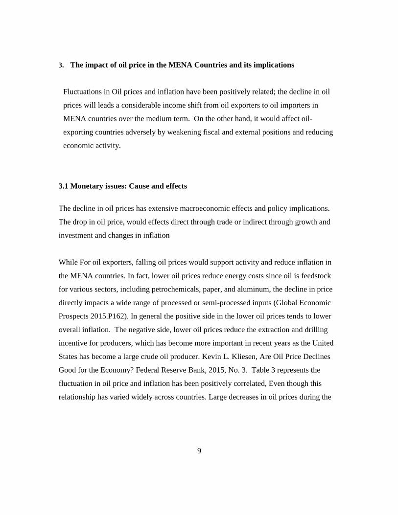
Fluctuations in Oil prices and inflation have been positively related; the decline in oil

prices will leads a considerable income shift from oil exporters to oil importers in

MENA countries over the medium term. On the other hand, it would affect oil-

exporting countries adversely by weakening fiscal and external positions and reducing

economic activity.

3.1 Monetary issues: Cause and effects

The decline in oil prices has extensive macroeconomic effects and policy implications.

The drop in oil price, would effects direct through trade or indirect through growth and

investment and changes in inflation

While For oil exporters, falling oil prices would support activity and reduce inflation in

the MENA countries. In fact, lower oil prices reduce energy costs since oil is feedstock

for various sectors, including petrochemicals, paper, and aluminum, the decline in price

directly impacts a wide range of processed or semi-processed inputs (Global Economic

Prospects 2015.P162). In general the positive side in the lower oil prices tends to lower

overall inflation. The negative side, lower oil prices reduce the extraction and drilling

incentive for producers, which has become more important in recent years as the United

States has become a large crude oil producer. Kevin L. Kliesen, Are Oil Price Declines

Good for the Economy? Federal Reserve Bank, 2015, No. 3. Table 3 represents the

fluctuation in oil price and inflation has been positively correlated, Even though this

relationship has varied widely across countries. Large decreases in oil prices during the

9

http://research.stlouisfed.org/econ/kliesen/

last three years were often followed by cycles of low inflation for instance, Jordan as in

many other countries, Sustained low oil prices are likely to have significant implications.

Table 3

Inflation rate in the MENA Countries %

& oil price (2013-3015)

Country

Oil price$/b

2013

105.9

2014

96.2

2015

41.8

Jordan UAE

Bahrain Tunisia Algeria Djibouti

Saudi Arabia Sudan Iraq

Oman Qatar

Qumran Kuwait

Lebanon Libya Egypt

Morocco Mauritania

Yemen

5.60 1.01 3.31 5.80 3.26 2.40 3.50

37.10 1.88 1.10 3.07 2.30 2.71 3.20 2.60 6.92 1.88 4.13

11.20

3.00 1.11 3.00 4.90 2.92 2.90 2.60

37.50 2.24 1.00 3.00 1.50 2.91 1.50 3.10

10.10 0.40 4.40 8.60

2.10 1.42 3.00 4.90 3.00 1.50 2.70

25.90 4.00 1.00 3.50 2.00 3.50 2.00 6.00 9.50 1.40 4.30

10.00

MENA 5.09 4.27 4.14

Source: The prospects of the Arab Economy Report 2015

3.2. Fiscal aspects: Challenges and opportunities

The decline in oil prices will have major effects in fiscal and external debts, in oil-

exporting and importing countries.

10

With regard to the fiscal matters, the loss in oil revenues for exporters will damage public

finances, while savings among oil importers could help rebuild fiscal space. Current

account balances are expected to improve in oil-importing countries and deteriorate in

oil-exporting countries.

Table 4

Deficit / Surplus General Budget as a percentage of GDP

In the MENA Countries + oil prices (2013-2015) Country

Oil price$/b 2013

105.9

2014

96.2

2015

41.8

Jordan -5.55 -3.50 -2.50

UAE 2.31 6.00 -3.50

Bahrain -3.31 -5.40 -10.00

Tunisia -5.20 -4.90 -4.90

Algeria -1.40 -7.40 -21.67

Djibouti 1.25 -3.10 -1.90

Saudi.Arabia 6.50 -2.30 -4.97

Sudan -2.94 -2.50 -3.20

Iraq 2.50 -5.00 -9.08

Oman 1.16 -1.00 -8.00

Qatar 14.20 12.20 8.70

Kuwait 25.89 22.00 -16.05

Lebanon -9.32 -9.50 -9.00

Libya -1.90 -40.00 -30.00

Egypt -13.67 -12.00 -10.50

Morocco -6.31 -5.10 -4.30

Mauritania -1.15 -0.40 -1.50

Yemen -8.33 -5.00 -7.00

MENA 2.93 -1.18 -6.90

Source: The prospects of the Arab Economy Report.2015 11

A number of MENA countries provide large fuel subsidies totheir populations. In some

cases, the cost of subsidies exceeds %5 of GDP, which leads to Savings on subsidies

(Energy subsidies2014) Although Fiscal deficits are expected to remain high with MENA

importers countries in the medium-term.

While lower oil prices presents an opportunity to implement structural reforms (World

Bank March, 2015).The revenue structure of oil exporting countries is dominated large

oil sectors.

Table 4 represents that, both oil exporters and importers have been affected by the recent

sharp drop in oil prices, for some importers, the deficit was lower in 2015 after the oil

shock than before.

In general the table indicated, the MENA countries in 2015 was suffering from high

deficit except Qatar was estimated a surplus and mostly due to the large dependence in

producing natural gas.

In order to understand other fundamental economic indicators of the MENA countries from

the view of government net debt and external debt related to the economic growth and the

effects of oil price, which classified differently oil importers from exporters.

Table 5 represents that, MENA exporters in the period of oil drop this has not affected on

the economic growth as well as the government dept but the External Debt would be

increased in the short run.

While the GDP for the MENA importers were increasing by the lower oil prices, this would

be considered as economic activity to the importers and could be activated their growth.

While for the importers on the long run would reduce the External Debt. The impact of the

low oil prices for the exporters on long time may dampen economic activity.

12

Table 5

Real GDP Growth, Government, External Debt MENA Countries %

Oil

price $/b

2013 2014 2015

105.9 96.2 41.8

MENA GDP 2.2 2.8 3.3

Oil exporters

Total Government -15.8 7.2 7.4

Net Debt

Total Gross 26.2 26.6 29.3

External Debt

MENA GDP 3.0 3.0 3.9

Oil importer

Total Government 68.8 70.3 70.8

Net Debt

Total Gross 36.3 36.0 35.5

External Debt

Source:IMF, Statistical Appendix, 2015

In several oil exporters that have not been able to accumulate substantial resources, will

face substantial pressures on their budgets, for instance Iraq and the severe damage in the

budget because of dependency on oil sector.

3.3 The role of MENA oil importers in strengthening a dual economic growth

The impact of the MENA countries and the economic growth on oil price can

be seen in the light of GDP as one of the main determinants of oil demand, in the MENA

countries, oil prices tend to be fluctuating, due to the differences in the business cycle,

unexpected economic growth has an important impact on oil demand

13

In the Middle East and North Africa, the potential gross domestic product improvements

in the region offer some upside in oil demand. Egypt one of the region’s largest

economies is forecast to recover well in the medium-term and support regional growth.

Ongoing challenges, the domestic oil demand also would be affecting due to the

geopolitical developments in the region. Hence, average GDP growth rates scenarios for

the period 2016–2020 is estimated the higher economic growth is %3.6 and increase the

oil demand to 12.8 mb/d (World Oil Outlook 2015).

Oil prices then, tend to be fluctuating, due to differences in the business cycle for that

reason, unexpected economic events have an important impact on oil demand this can be

viewed in the fact that the most recent global financial crisis has had significant

implications on oil demand projections. Back in 2008, before the severity of the crisis

became evident, oil demand projections for 2015 in the *WOO were at around 96 mb/d.

However, demand projections for 2015 in the WOO 2009 and the WOO 2010, which

assumed significantly lower GDP growth, were reduced to 90 mb/d and 91 mb/d,

respectively (World Oil Outlook 2015).

14

Table 6

Gross domestic product % and oil demand in the MENA Countries

mb/d (2009 -2020)

Prepared

by the researcher/ based on:

- AOPEC, the secretary-general's Annual report 40

- OPEC Monthly Oil Market Report – November 2015

- OPEC Monthly Oil Market Report – January 2016

- OPEC World Oil Outlook 2015

Therefore, the Impact of drop oil price, should be strengthening the economic growth in

importers since economic activity in these countries would generate more oil demand,

thus would furthermore enhancing another economic growth to the exporting countries.

In this case the impact of low oil price would work as dual effects by stimulating the

economic growth in both sides

Table 6 represents that GDP is increasing in each oil price drop; it would generates more

oil demand from the MENA countries especially from oil importers. Although the

projection of oil price predicted to be $80b/d but there is a trend that GDP would be 3.6

more than the previous period.

4. The reliability of oil price in affecting the gross domestic product in

MENA countries

During the half quarter of 2014, the world has experience low oil prices the extreme

fluctuation of what is consider of an oil shock in the global economy. This has been

raised a very fundamental question? How much is reliable oil price in affecting economic

growth in MENA countries, and led predicting variation in GDP growth remains a

15

controversial issue. Several models have been developed targeting different relations

between oil price and GDP growth according to its effects on oil markets. Other variables

MENA 2009 2010 2011 2012 2013 2014 2015 2020

GDP 3.0 5.5 3.9 4.6 2.1 2.6 3.2 3.6

Oil Demand 10.3 10.6 10.7 11.0 11.3 11.84 12.21 12.8

Oil price $/b 61.0 77.4 107.5 109.5 105.9 96.2 41.8 80

may have dominated role and led to consequences in gross domestic product. Policy

makers face a dual challenge one in adjusting to lower oil prices and dealing with

security risks in the short run, and boost growth and employment in the long run,

moreover, the large role played by governments in these economies, make economic

adjustment more difficult.(Global-Economic-Prospects2015)

The research approached different statistical test, Panel-data unit-root tests, cointegration

model, and Panel Dynamic Least Squares (PDOLS) are taken part of this section. The

sample was extended to include (17) countries of the Middle East and North Africa, data

of the research is from 2009 to 2015.

The causality relationship between different time series is based on:

GDP = F (P, K, L)

While: P is to explain the oil price, K for the fixed capital and L for the labor are

explained as independent variable, while GDP is the dependent variable. to investigate

the relationship between the variables that mentioned the research approached different

tests to search for stationarity or non-stationarity of the cross section time series,

different tests of the unit root and the cointegrating model were applying, to avoid the

problematic which related in the explanatory variables in explaining their impacts on

GDP through the oil shocks

4.1. The Levin–Lin–Chu

4.2. Im–Pesran–chin




16

4.1. The Levin–Lin–Chu (2002)

Started with *GDP variable the estimation which has been indicated, the null hypothesis

which means that, the series contains a unit root:

Since H0: series imply a unit root (-15.9442) under the probability (0.00000)

So the hypothesis would be rejected. And the series is stationary. This should go to the

alternative hypothesis H1: to confirm the relation between the variables and its efect.

The Levin–Lin–Chu test assumes a common autoregressive parameter for all panels, so

this test does not allow, the dependent variable GDP explains the changes would happen

into independent variables, in other words to expose the causality of oil prices, labor and

fixed capital on gross domestic product in the MENA at short time, there might be

structural breaks that are causing the problem with the unit root test due to the Probability

that some countries within the sample contain unit roots, while other countries do not,

since the sample of the data imply exporters and importers

4.2. Im–Pesran–chin test where applied to the MENA countries data to examine whether

the series contains a unit root or not; the results were in the same direction of the first root

test that also it contains a unit root.

Moreover, the research runs the same previous tests for fixed capital (K) as well as for

the labor (L), where both are in the direction of H0: hypothesis, the series also contains a

unit root, and for the exporters. Except that the labor force would not change in the short

run in spite of lower oil price.

While the results in the table 7 of The Levin–Lin–Chu test for the oil price (P) proved

that the oil price is affecting the (GDP) in the MENA countries

* See the Annex

17

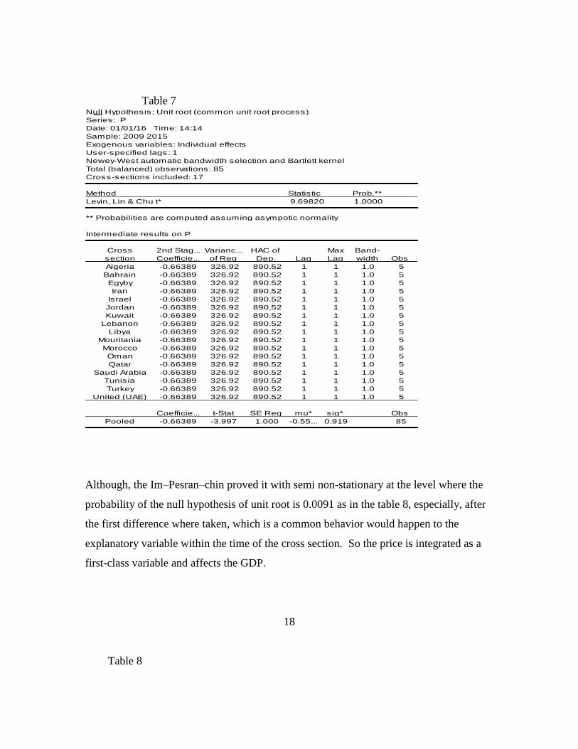
Table 7 Null Hypothesis: Unit root (common unit root process)

Series: P

Date: 01/01/16 Time: 14:14

Sample: 2009 2015

Exogenous variables: Individual effects

User-specified lags: 1

Newey-West automatic bandwidth selection and Bartlett kernel

Total (balanced) observations: 85

Cross-sections included: 17

Method Statistic Prob.**

Levin, Lin & Chu t* 9.69820 1.0000

** Probabilities are computed assuming asympotic normality

Intermediate results on P

Cross 2nd Stag... Varianc... HAC of Max Band-

section Coefficie... of Reg Dep. Lag Lag width Obs

Algeria -0.66389 326.92 890.52 1 1 1.0 5

Bahrain -0.66389 326.92 890.52 1 1 1.0 5

Egyby -0.66389 326.92 890.52 1 1 1.0 5

Iran -0.66389 326.92 890.52 1 1 1.0 5

Israel -0.66389 326.92 890.52 1 1 1.0 5

Jordan -0.66389 326.92 890.52 1 1 1.0 5

Kuwait -0.66389 326.92 890.52 1 1 1.0 5

Lebanon -0.66389 326.92 890.52 1 1 1.0 5

Libya -0.66389 326.92 890.52 1 1 1.0 5

Mouritania -0.66389 326.92 890.52 1 1 1.0 5

Morocco -0.66389 326.92 890.52 1 1 1.0 5

Oman -0.66389 326.92 890.52 1 1 1.0 5

Qatar -0.66389 326.92 890.52 1 1 1.0 5

Saudi Arabia -0.66389 326.92 890.52 1 1 1.0 5

Tunisia -0.66389 326.92 890.52 1 1 1.0 5

Turkey -0.66389 326.92 890.52 1 1 1.0 5

United (UAE) -0.66389 326.92 890.52 1 1 1.0 5

Coefficie... t-Stat SE Reg mu* sig* Obs

Pooled -0.66389 -3.997 1.000 -0.55... 0.919 85

Although, the Im–Pesran–chin proved it with semi non-stationary at the level where the

probability of the null hypothesis of unit root is 0.0091 as in the table 8, especially, after

the first difference where taken, which is a common behavior would happen to the

explanatory variable within the time of the cross section. So the price is integrated as a

first-class variable and affects the GDP.

18

Table 8

Null Hypothesis: Unit root (individual unit root process)

Series: P

Date: 01/01/16 Time: 14:15

Sample: 2009 2015





Method Statistic Prob.*...

Im, Pesaran and Shin W-stat 2.39417 0.991...


Intermediate ADF test results

Cross Max

section t-Stat Prob. E(t) E(Var... Lag Lag Obs

Algeria -0.6131 0.7773 -1.55... 2.64... 1 1 5

Bahrain -0.6131 0.7773 -1.55... 2.64... 1 1 5

Egyby -0.6131 0.7773 -1.55... 2.64... 1 1 5

Iran -0.6131 0.7773 -1.55... 2.64... 1 1 5

Israel -0.6131 0.7773 -1.55... 2.64... 1 1 5

Jordan -0.6131 0.7773 -1.55... 2.64... 1 1 5

Kuwait -0.6131 0.7773 -1.55... 2.64... 1 1 5

Lebanon -0.6131 0.7773 -1.55... 2.64... 1 1 5

Libya -0.6131 0.7773 -1.55... 2.64... 1 1 5

Mouritania -0.6131 0.7773 -1.55... 2.64... 1 1 5

Morocco -0.6131 0.7773 -1.55... 2.64... 1 1 5

Oman -0.6131 0.7773 -1.55... 2.64... 1 1 5

Qatar -0.6131 0.7773 -1.55... 2.64... 1 1 5

Saudi Arabia -0.6131 0.7773 -1.55... 2.64... 1 1 5

Tunisia -0.6131 0.7773 -1.55... 2.64... 1 1 5

Turkey -0.6131 0.7773 -1.55... 2.64... 1 1 5

United (UAE) -0.6131 0.7773 -1.55... 2.64... 1 1 5

Average -0.6131 -1.55... 2.648

Warning: for some series the expected mean and variance for the given lag

and observation are not covered in IPS paper


By using the Kao cointegration test the table represents that, this statistical method

represents a successful integrated where the tests indicated the presence of cointegration

between the variables (P, K, L) are affecting GDP. In spite of it might be co-integrated

about (0.0548).

19


The result of Augmented Dickey–Fuller (ADF) method, this test detects the presence or

absence of a unit root. In other words indicated that, this is non-stationary statistical

series. As the three independent variables (P, K, L) were verified and affected the

dependent variable (GDP), this concludes the return causality feedback causality between

the variables. As in the table 9.

Table 9

Kao Residual Cointegration Test

Series: GDP K L P

Date: 01/01/16 Time: 14:30

Sample: 2009 2015

Included observations: 119

Null Hypothesis: No cointegration

Trend assumption: No deterministic trend

User-specified lag length: 1


t-Statistic Prob.

ADF -1.600299 0.0548

Residual variance 320.1845

HAC variance 90.38572

Augmented Dickey-Fuller Test Equation

Dependent Variable: D(RESID)

Method: Least Squares

Date: 01/01/16 Time: 14:30

Sample (adjusted): 2011 2015

Included observations: 85 after adjustments

Variable Coefficient Std. Error t-Statistic Prob.

RESID(-1) -1.843437 0.171282 -10.76260 0.0000

D(RESID(-1)) 0.343435 0.105119 3.267095 0.0016

R-squared 0.725502 Mean dependent var 0.380582

Adjusted R-squared 0.722194 S.D. dependent var 20.70849

S.E. of regression 10.91488 Akaike info criterion 7.641379

Sum squared resid 9888.172 Schwarz criterion 7.698853

Log likelihood -322.7586 Hannan-Quinn criter. 7.664497

Durbin-Watson stat 2.433090

The ²R estimated as an appropriate result, more than %72 of independent variables of (P,

K, L) explained the change in dependent variable of GDP. With acceptance of null

hypothesis, (T-statistic and Durbin-Watson) as well.

20


In the light of the previous results and by using the Panel Dynamic Least Squares

(PDOLS) method in order to describe the change of the independent variables over time,

by considering a constant and non constant, linear trend and Quadratic trend to explain a

long term tendency.

The results-table 10 indicated that the coefficient of the MENA variables are statistically

significant in all regressions the variable of oil price and its impact was negative in all

regressions agreed with economic theory and statistically was significant in the Quadratic

trend.

Table 10

Dependent Variable: GDP

Method: Panel Dynamic Least Squares (DOLS)

Date: 01/02/16 Time: 13:33

Sample: 2009 2015

Periods included: 7


Total panel (balanced) observations: 119

Panel method: Pooled estimation

Cointegrating equation deterministics: C @TREND @TREND^2

Static OLS leads and lags specification

Coefficient covariance computed using sandwich method

Long-run variances (Bartlett kernel, Newey-West fixed bandwidth) used for

coefficient covariances

No d.f. adjustment for standard errors & covariance


K 7.668370 1.985661 3.861873 0.0003

L 19.81325 3.654722 5.421275 0.0000

P -0.169670 0.059136 -2.869173 0.0055


Adjusted R-squared -0.197148 S.D. dependent var 11.92045

S.E. of regression 13.04267 Sum squared resid 11057.23

Durbin-Watson stat 2.922007 Long-run variance 21.53115

This concludes that, the effects of oil price in GDP would appears on the long run in the

MENA countries, but it should be noted that, as this has not yet translated into stronger

economic growth.

21

5. Conclusion

This paper has estimated the effects of oil price shocks on the economic activity of the

Middle East and North Africa, and focuses on the relationship between oil price and GDP

growth, which analyzed in terms of, Panel-data unit-root tests, cointegration model, and

Panel Dynamic Least Squares (PDOLS). This relationship examined by the unit-root

approach, in which oil prices are assumed to have consistent impacts on economic growth

and this came to conclusion that, the oil prices affected the gross domestic product, which

explains the effective role of the oil price as an independent variable on the GDP as a

dependent variable.

Moreover, it concluded that, by the (ADF) method the interaction between oil variable

and other macroeconomic variables, as fixed capital and labor are found to be

fundamental factors by explaining the change in GDP.

While the further statistic methods such as, Levin–Lin–Chu and the Im–Pesran–chin,

they have not shown a clear impact from fixed capital and labor on GDP and vice versa.

As the consequences of the continuation effects of oil prices, have a completely different

behavior in each oil shock, the results of the Ordinary least squares (OLS) of OPEC

model as well as world oil demand and oil production models, indicates the action of oil

price throughout the 1970s and its effects on world oil demand was positively related,

which is completely contrary to the economic theory. While in the 1980s world oil

demand led the OPEC production done, regardless, of oil price role. In other words oil

price factor disappeared in affecting OPEC oil. Besides, non-conformity with the

economic theory and despite of that OPEC production was acceded, thus led to a series of

declines in oil prices till-1990s.

While the cause of the fall in oil prices 2014-2015 it was similar to the oil shock in 1985-

1986 due to the estimation, caused by the supply glut as well, but differed this time as it

is from non-OPEC countries.

While the cause of the fall in oil prices 2014-2015, due to the estimation, it is similar to

the oil shock in 1985-1986, caused by the supply glut as well, but this time differed

from the past since it is for non-OPEC countries

22

6. References

Global-Economic-Prospects, 2015 June, Middle-East-and-North-Africa-analysis, P5

Hussein Abdullah, 2000, the future of the Arab oil magazine, Beirut, November, PP28-31

John Kingston 2015 September7, Paper and barrels, pushing and pulling oil prices:

Petrodollars

http://blogs.platts.com/2015/09/07/paper-barrels-oil-prices-petrodollars/

Hedging against Falling Crude Oil Prices using Crude Oil Futures, The

OptionsGuide.com, 2009

http://www.theoptionsguide.com/crude-oil-futures-short-hedge.aspx

The World Oil Market Current Conditions and Immediate Prospects, September 2003

Report to the100th Meeting of the Economic Commission Board, OPEC Secretariat,

P.32.

Prices Glossary, 2000, International Energy Agency, August, p44

OPEC Monthly Oil Market Report November 2015, PP.6-.91

OPEC, World Oil Outlook 2015, PP 182-184

John Baffes; AyhanKose, 2015 January understanding the plunge in oil prices: Sources

and implications, World Bank, Global Economic Prospects P159

World Bank Group, 2015 March, The Great Plunge in Oil Prices: Causes, Consequences,

and Policy Responses, PP5-6.

David Hough; Cassie Barton, 14 January 2016, No 04153, House of Commons, p5.

OPEC Monthly oil market Report18 January 2016

OPEC Monthly Report, Jan 2016. P46

OPEC, Annual Statistical Bulletin 2015, 50th edition PP42-28

Zhenbo Hou, Jodie Keane, March 2015, the oil price shock of 2014 Drivers, impacts and

policy implication. Working paper 415, P11

http://www.odi.org/sites/odi.org.uk/files/odi-assets/publications-opinion-files/9589.pdf

Kevin L. Kliesen, 2015, Are Oil Price Declines Good for the Economy? Federal Reserve

Bank, No. 3.

The prospects of the Arab economy report, 2015, PP55-57

IMF, Statistical Appendix, 2015

AOPEC, the secretary-general's Annual report 40

23

OPEC Monthly Oil Market Report – November 2015

http://blogs.platts.com/2015/09/07/paper-barrels-oil-prices-petrodollars/

http://www.odi.org/sites/odi.org.uk/files/odi-assets/publications-opinion-files/9589.pdf

http://research.stlouisfed.org/econ/kliesen/

Energy subsidies in the Middle East and North Africa lessons for reform March, 2014 https://www.imf.org/external/np/fad/subsidies/pdf/menanote.pdf

OPEC World Oil Outlook 2015 PP48-46-85

Journal of Oil and Industry News, United Arab Emirates, Abu Dhabi 273 Issue, May

1993, P2

Unified Arab Economic Report - 1991, 1990

OAPEC Reports 1988, 1991

Follow – up activities of the energy sources of Arab and International 1992-1993

World oil trends, Cambridge Energy Research, 1988-1989

World Economic Form The global Competitiveness Report, (2009-2010)

(2010-2011),(2011-2012),(2012-2013),(2013-2014),

(2014-2015) (2015-2016)

International Monetary Fund April 2015

World Economic Situation and prospects 2015

OAPFC, the Secretary Generals 41 Annual Report, 2014

World Economic situation and prospects 2012

ESCWA, National Accounts studies of the Arab Region , Bulletin

No .33 , New York , 2013

24

Annex

Table 1 world oil demand model

D.W F Rˉ²

(%)

R² (%) The mathematical form of the function Years Function Type

0.30

0.35

0.32

0.63

0.86

0.87

0.91

1.14

1.22

16.04

19.3

15.94

70.35

52.79

45.96

58.01

57.01

48.26

44.2

49.0

44.0

88.0

84.5

82.6

90.0

89.8

88.2

47.13

51.74

46.97

89.22

86.13

84.39

91.58

91.44

90.05

Y2=31.01-0.65x3

(-4.01)

Y2=34.69-11.41logx3 (-4.39)

logY2=1.556-0.194logx3

Y2=-58.28-1.30x3+1.57x2

(-11.84) (8.15)

Y2=-2.9284-2.0logx3+1.88logx2

(-10.25) (6.49)

lohY2=-4.719-0.36logx3+3.60logx2

(-9.59) (6.38) Y2=-49.96-1.19x3+1.45x2-0.11x1

(-10.74) (7.87) (-2.12)

Y2=3.6591-2.60logx3+2.28logx2+8.4logx1 (-10.51) (8.55) (3.15)

logY2=6.1650.477logx3+4.36logx2+0.158logx1

(-9.76) (8.25) -(3.02)

1973-1992

1973-1992

1973-1992

1973-1992

1973-1992

1973-1992

1973-1992

1973-1992

1973-1992

Linear

Half logarithmic

Double logarithmic

Linear

Half logarithmic

Double logarithmic

Linear

Half logarithmic

Double logarithmic

Source: computed Time X3 oil demand X2 oil price X1 OPEC production Y1

Table 2 OPEC oil demand model D.W F Rˉ²(%) R²(%) 0.30

0.79

0.78

1.35

1.06

1.06

16.04

17.52

17.77

28.96

17.6

17.99

44.2

46.5

46.9

74.6

63.6

67.91

47.13

49.33

49.68

77.31

67.43

64.6

Y1=31.01-0.65*3

(-4.01) Y1=-94.45+87.0 log x2

(4.19)

logY1=0.65985+0.63 log x2 (4.22)

Y1=-3.527+1.11 x2 -0.388 x3

(7.51) (-4.64) logY1=1.773+1.35logx2-4.8logx3

(5.8) (-3.07)

logY1=0.05985+0.98logx2-0.35logx3 (5.87) (-3.11)

1992-1973

1992-1973

1992-1973

1992-1973

1992-1973

1373-1992

Linear

Half logarithmic

Double logarithmic

Linear

Double logarithmic

Double logarithmic

Source: Author calculation Oil production Oil demand Time variables

25

Table 3 OPEC oil production model 73-1985

D.W F Rˉ²

(%)

R²

(%)

OPEC oil production model 73-1985

Mathematical function form

Years Type of the

function

0.58

0.39

0.32

2.54

1.06

0.94

0.99

1.05

37.99

12.16

11.63

25.49

30.65

24.53

30.35

28.61

77.0

48.2

47.0

97.7

83.2

79.7

88.0

87.3

77.55

52.54

51.39

98.08

85.97

83.07

91.0

90.51

Y2=35.65-1.405x3

(-6.16)

Y2=36.03-13.51logx3

(-3.49)

logY2=1.586-0.249logx3

(-3.41)

Y2=-31.74-1.595x3+1.16x2

(-22.05) (10.33)

Y2—347.29-18.8logx3+21.81logx2

(-7.04) (4.88)

logY2=-5.350-0.344logx3+3.95logx2

(-6.85) (4.33)

Y2=-4.135-3.1logx3+2.52logx2+1.3logx1

(-5.32) (6.20) (2.24)

logY2=-6.847-0.62logx3+4.70logx2+0.30logx1

(-5.57) (6.70) (2.66)

1973-1985

1973-1985

1973-1985

1973-1985

1973-1985

1973-1985

1973-1985

1973-1985

Linear

Half logarithmic

Double logarithmic

Linear

Half logarithmic

Double logarithmic

Half logarithmic

Double logarithmic

Source: Computed Y2= OPEC production X1= Oil PriceX2= World oil demand X3=Time variables

Table 4 OPEC oil production model 86-1992

DW F Rˉ²% R² (%)

1.49

1.44

1.59

1.72

2.10

170.71

150.17

190.14

127.68

189.19

96.9

96.1

96.9

97.7

98.4

79.15

96.78

97.44

98.46

98.95

Y2=-39.30+0.945x2

(13.07)

Y2=-228.3+1.38logx2

(12.25)

logY2=3.848+2.86logx2

(13.79)

Y2=-390.01+2.29logx2-5.4logx3

(5.15) (-2.09)

LogY2=-7.024+4.56x2-0.105logx3

(6.14) (-241)

1986-1992

1986-1992

1986-1992

1986-1992

1986-1922

Linear

Half logarithmic

Double logarithmic

Half logarithmic

Double logarithmic

26

Annex for different tests Levin, lin, chu test

GDP variable


Series: GDP

Date: 01/01/16 Time: 14:06

Sample: 2009 2015






Im, Pesaran and Shin W-stat -4.90261 0.000...



Cross Max


Algeria -2.0265 0.2697 -1.55... 2.64... 1 1 5

Bahrain -1.5112 0.4495 -1.55... 2.64... 1 1 5

Egyby -3.0200 0.0961 -1.55... 2.64... 1 1 5

Iran -2.9218 0.1066 -1.55... 2.64... 1 1 5

Israel -2.6449 0.1410 -1.55... 2.64... 1 1 5

Jordan 5.4081 0.9999 -1.55... 2.64... 1 1 5

Kuwait -6.0191 0.0074 -1.55... 2.64... 1 1 5

Lebanon -23.325 0.0000 -1.55... 2.64... 1 1 5

Libya -2.0576 0.2610 -1.55... 2.64... 1 1 5

Mouritania -4.8870 0.0177 -1.55... 2.64... 1 1 5

Morocco -0.8044 0.7242 -1.55... 2.64... 1 1 5

Oman -2.2906 0.2030 -1.55... 2.64... 1 1 5

Qatar -2.8637 0.1132 -1.55... 2.64... 1 1 5

Saudi Arabia -1.8628 0.3199 -1.55... 2.64... 1 1 5

Tunisia -1.9552 0.2909 -1.55... 2.64... 1 1 5

Turkey -4.6674 0.0212 -1.55... 2.64... 1 1 5

United (UAE) -1.9307 0.2979 -1.55... 2.64... 1 1 5

Average -3.4929 -1.55... 2.648


and observation are not covered in IPS paper im, pesran, chin test

Null Hypothesis: Unit root (common unit root process)

Series: GDP

Date: 01/01/16 Time: 14:01

Sample: 2009 2015







Levin, Lin & Chu t* -15.9442 0.0000


Intermediate results on GDP



Algeria -1.74508 0.0975 1.4856 1 1 0.0 5

Bahrain -1.43955 1.2121 0.8458 1 1 5.0 5

Egyby -1.33263 0.4723 1.9211 1 1 1.0 5

Iran -1.42367 5.9663 5.7534 1 1 5.0 5

Israel -0.60292 0.0518 1.9048 1 1 4.0 5

Jordan 1.28968 0.0031 1.7414 1 1 0.0 5

Kuwait -1.44352 1.7904 24.302 1 1 3.0 5

Lebanon -1.26215 0.0348 6.1511 1 1 2.0 5

Libya -2.26980 1749.0 864.92 1 1 5.0 5

Mouritania -1.01006 0.0452 3.9202 1 1 1.0 5

Morocco -0.75062 0.1519 0.8721 1 1 2.0 5

Oman -2.00314 0.5080 0.4176 1 1 5.0 5

Qatar -0.71348 1.7663 3.2884 1 1 5.0 5

Saudi Arabia -1.33567 4.0924 4.3517 1 1 5.0 5

Tunisia -2.05515 2.5035 1.4653 1 1 5.0 5

Turkey -1.90746 1.2414 12.717 1 1 4.0 5

United (UAE) -0.82467 0.3859 8.0633 1 1 0.0 5


Pooled -1.12501 -17.593 2.179 -0.55... 0.919 85

27

Levin, lin, chu test

Fixed capital Null Hypothesis: Unit root (common unit root process)

Series: K

Date: 01/01/16 Time: 14:09

Sample: 2009 2015







Levin, Lin & Chu t* -7.34763 0.0000


Intermediate results on K



Algeria -0.72115 0.0021 0.0314 1 1 5.0 5

Bahrain -0.88189 0.0019 0.0044 1 1 1.0 5

Egyby -0.64287 0.0019 0.0227 1 1 2.0 5

Iran -0.45158 0.0004 0.0046 1 1 1.0 5

Israel -1.65328 0.0008 0.0325 1 1 2.0 5

Jordan -1.80114 0.0058 0.0113 1 1 3.0 5

Kuwait -1.50057 0.0015 0.0048 1 1 4.0 5

Lebanon -0.65924 0.6228 0.2432 1 1 5.0 5

Libya -2.16081 0.4314 0.2546 1 1 5.0 5

Mouritania -1.44240 0.0122 0.0081 1 1 5.0 5

Morocco -0.19370 0.0001 0.0087 1 1 0.0 5

Oman -1.75668 0.0114 0.0178 1 1 0.0 5

Qatar 0.28623 0.0156 0.0170 1 1 5.0 5

Saudi Arabia -1.32683 0.0021 0.0326 1 1 1.0 5

Tunisia -1.44176 0.8232 0.3697 1 1 5.0 5

Turkey -0.97039 0.0023 0.0185 1 1 1.0 5

United (UAE) -1.65887 0.0102 0.0201 1 1 5.0 5


Pooled -0.33346 -8.492 1.645 -0.55... 0.919 85 im, pesran, chin test


Series: K

Date: 01/01/16 Time: 14:10

Sample: 2009 2015









Cross Max


Algeria -2.6024 0.1472 -1.55... 2.64... 1 1 5

Bahrain -1.4857 0.4599 -1.55... 2.64... 1 1 5

Egyby -5.2012 0.0137 -1.55... 2.64... 1 1 5

Iran -4.4593 0.0253 -1.55... 2.64... 1 1 5

Israel -3.5625 0.0566 -1.55... 2.64... 1 1 5

Jordan -1.7785 0.3497 -1.55... 2.64... 1 1 5

Kuwait -4.6071 0.0223 -1.55... 2.64... 1 1 5

Lebanon -0.2792 0.8584 -1.55... 2.64... 1 1 5

Libya -1.9487 0.2932 -1.55... 2.64... 1 1 5

Mouritania -1.6918 0.3799 -1.55... 2.64... 1 1 5

Morocco -4.2969 0.0291 -1.55... 2.64... 1 1 5

Oman -1.2621 0.5543 -1.55... 2.64... 1 1 5

Qatar 0.3962 0.9525 -1.55... 2.64... 1 1 5

Saudi Arabia -1.5272 0.4433 -1.55... 2.64... 1 1 5

Tunisia -1.6520 0.3953 -1.55... 2.64... 1 1 5

Turkey -2.4479 0.1714 -1.55... 2.64... 1 1 5

United (UAE) -2.2274 0.2175 -1.55... 2.64... 1 1 5

Average -2.3902 -1.55... 2.648


and observation are not covered in IPS paper

28

Null Hypothesis: Unit root (common unit root process)

Series: L

Date: 01/01/16 Time: 14:12

Sample: 2009 2015







Levin, Lin & Chu t* -9.07954 0.0000


Intermediate results on L



Algeria -1.00568 0.0115 0.0321 1 1 5.0 5

Bahrain -1.53472 0.0034 0.0096 1 1 1.0 5

Egyby -0.71375 0.0006 0.0124 1 1 0.0 5

Iran -1.30281 0.1133 0.0650 1 1 5.0 5

Israel -0.82566 0.0006 0.0139 1 1 3.0 5

Jordan -0.70000 0.0005 0.0004 1 1 5.0 5

Kuwait -0.01528 0.0121 0.0033 1 1 5.0 5

Lebanon -0.56950 0.1765 0.3791 1 1 0.0 5

Libya -1.06512 0.8791 0.2683 1 1 5.0 5

Mouritania -0.09699 0.0088 0.0018 1 1 5.0 5

Morocco -1.20907 0.0424 0.0829 1 1 0.0 5

Oman 1.44171 0.0450 0.1098 1 1 1.0 5

Qatar -3.91337 0.0076 0.1663 1 1 2.0 5

Saudi Arabia -1.30247 0.0849 0.0407 1 1 5.0 5

Tunisia 0.24537 0.0040 0.0162 1 1 1.0 5

Turkey -2.20041 0.0042 0.0061 1 1 5.0 5

United (UAE) -0.87422 0.0181 0.0081 1 1 5.0 5


Pooled -0.70301 -10.270 1.700 -0.55... 0.919 85


Series: L

Date: 01/01/16 Time: 14:13

Sample: 2009 2015









Cross Max


Algeria -3.9947 0.0381 -1.55... 2.64... 1 1 5

Bahrain -2.0265 0.2697 -1.55... 2.64... 1 1 5

Egyby -6.0363 0.0073 -1.55... 2.64... 1 1 5

Iran -1.5585 0.4312 -1.55... 2.64... 1 1 5

Israel -7.9667 0.0022 -1.55... 2.64... 1 1 5

Jordan -1.9540 0.2912 -1.55... 2.64... 1 1 5

Kuwait -0.0395 0.9018 -1.55... 2.64... 1 1 5

Lebanon -0.4911 0.8082 -1.55... 2.64... 1 1 5

Libya -0.9626 0.6709 -1.55... 2.64... 1 1 5

Mouritania -0.4183 0.8261 -1.55... 2.64... 1 1 5

Morocco -1.3720 0.5073 -1.55... 2.64... 1 1 5

Oman 0.3223 0.9460 -1.55... 2.64... 1 1 5

Qatar -6.2847 0.0062 -1.55... 2.64... 1 1 5

Saudi Arabia -1.2555 0.5571 -1.55... 2.64... 1 1 5

Tunisia 1.0451 0.9843 -1.55... 2.64... 1 1 5

Turkey -3.4912 0.0606 -1.55... 2.64... 1 1 5

United (UAE) -1.4769 0.4637 -1.55... 2.64... 1 1 5

Average -2.2330 -1.55... 2.648


and observation are not covered in IPS paper 29



Date: 01/02/16 Time: 13:35

Sample: 2009 2015

Periods included: 7










K -0.208113 1.121630 -0.185545 0.8531

L 1.685759 1.500185 1.123700 0.2635

P -0.023721 0.030498 -0.777789 0.4383







Date: 01/02/16 Time: 13:36

Sample: 2009 2015

Periods included: 7




Cointegrating equation deterministics: C







K 7.287657 2.758409 2.641979 0.0096

L 8.868682 3.791444 2.339131 0.0213

P -0.010384 0.030116 -0.344812 0.7310





30



Date: 01/02/16 Time: 13:37

Sample: 2009 2015

Periods included: 7




Cointegrating equation deterministics: C @TREND







K 9.356136 2.986142 3.133185 0.0024

L 12.86508 4.931095 2.608970 0.0108

P -0.018544 0.028053 -0.661043 0.5104







Date: 01/02/16 Time: 13:33

Sample: 2009 2015

Periods included: 7




Cointegrating equation deterministics: C @TREND @TREND^2







K 7.668370 1.985661 3.861873 0.0003

L 19.81325 3.654722 5.421275 0.0000

P -0.169670 0.059136 -2.869173 0.0055





31

the impact of oil shocks on the economic growth in the ... · world oil demand, production (mb/d)...

Documents