The Impact of Liquidity on Household Balance Sheets:Micro Responses to a Credit Card Supply Shock

Jonathan Zinman*

Federal Reserve Bank of New YorkJanuary 10, 2003

ABSTRACT

Despite growing evidence that many US households are liquidity constrained,there remains little consensus on the quantitative importance or nature of theseconstraints. This paper develops a new type of evidence on the impacts ofconsumer credit markets on behavior by examining household-level responses toan exogenous liquidity shock. A United States Supreme Court decisioneffectively deregulated bank credit card interest rates in December 1978, and Ifind that consumers from states with binding usury ceilings before the decisionbecame more likely to hold bank cards after the decision, relative to theircounterparts in unaffected states. The marginal cardholders appear to havecharacteristics widely associated with credit constraints, and to borrow frequentlyon their new cards. Yet there is little evidence that these cardholders exploit theirnewfound liquidity by shifting into higher-yielding, less liquid, or riskier assets.This finding is at odds with standard models of liquidity constraints, andmotivates consideration of alternative explanations for the widely observedsensitivity of consumers to liquidity.

* Jonathan.Zinman@ny.frb.org; tel: 212-720-1204. I am particularly grateful to DaronAcemoglu and Jon Gruber for their guidance. The author also thanks Daniel Bennett and KurtJohnson for excellent research assistance, and Adam Ashcraft, Ricardo Caballero, KathleenJohnson, Jim Poterba, Phil Strahan, and participants in the MIT macro and public financelunches and the 2003 AEA Meetings for helpful comments. The views expressed do notnecessarily represent those of the Federal Reserve Bank of New York or of the Federal ReserveSystem.

2

I. Introduction

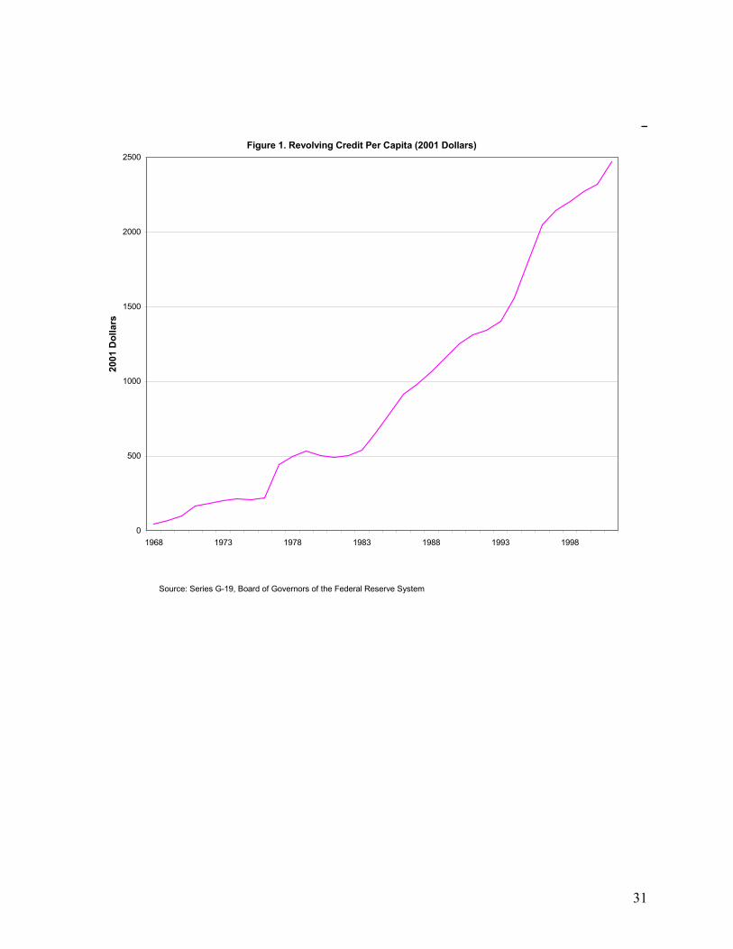
Consumer credit markets have grown dramatically over the last 30 years. Figure 1 shows

that revolving consumer credit outstanding in the United States has increased sixty-fold in real

terms since 1968. The development of bank credit cards has been a primary driver of this

growth. The proportion of households using these cards has risen from 0.07 in 1968 to 0.68 in

1998 (Kennickell, et. al. 2001) with year 2001 aggregate outstanding credit card balances

totaling about $600 billion (Board of Governors of the Federal Reserve System, 2002). This

equates to over $5500 per household and 6% of GDP.

Various literatures are concerned with the implications of this growth in consumer credit, but

fundamental puzzles remain. Growth could be caused by secular changes in demand for

liquidity, and/or by technological innovations that relax liquidity constraints. Disentangling the

roles of supply and demand in consumer credit markets has been a difficult task empirically, as

Gross and Souleles (2002) note. Not surprisingly, then, there is little consensus on the

quantitative importance of liquidity constraints and precautionary motives (Browning and

Lusardi 1996).

Of course the lack of obvious exogenous variation in access to liquidity has also frustrated

attempts to identify the effects of the growth of consumer credit. Meanwhile, interest in

estimating these effects has grown along with recent theoretical work showing that consumer

credit constraints have important implications. On the macro side, they can amplify business

cycles (Hubbard and Judd 1986) and retard growth (Jappelli and Pagano 1999). More

surprisingly, various works have shown that the welfare implications of expanded consumer

credit markets are ambiguous, given various types of incomplete markets or nonstandard

3

preferences.1 Interactions between easy credit and incomplete contracts can lead to social

welfare losses, as Athreya (2001) demonstrates for the case of bankruptcy law. Relaxing interest

rate ceilings to increase credit supply might reduce welfare if usury laws mitigate insurance

market failures (Glaeser and Scheinkman 1998), or combat lender market power (Blitz and

Long, 1965). Expanding consumer credit markets may provide “too much liquidity” if

consumers have self-control problems (Laibson 1997), leading consumers to underestimate their

credit card borrowing (Ausubel 1991) and/or to undersave (Laibson, Repetto, and Tobacman

1998). Any of these phenomena could produce optimization failures and result in welfare losses.

This paper develops new evidence on the causes and effects of liquidity growth by using the

deregulation of interest rate ceilings to help identify increases in bank card use. These increases

are arguably exogenous to credit demand and other unobservable determinants of household

behavior. I identify states that had a binding usury ceiling (“affected” states) prior to the 1978

Marquette Supreme Court case that deregulated bank card interest rates, and show that following

deregulation the proportion of households using bank cards increased in those states, relative to

“unaffected” states that did not have binding usury ceilings prior to the case. Consideration of

various potential confounds suggests that this result is not driven by unobservable differences

between affected and unaffected states (or across households therein). Changes in usury law

then can be used to identify the effects of shifts in access to credit on other margins of consumer

behavior, including portfolio and occupational choice. This paper is thus the first study to

exploit a plausibly exogenous shock to directly estimate effects of access to consumer credit on

these types of outcomes; i.e., on outcomes in addition to borrowing.2

1 With complete markets, consumer credit will expand if demand increases and/or lender costs decrease. In eithercase the expansion will be efficient.2 There is a small literature that does look specifically at the impact of credit card usury ceilings on card use(Dunkelberg, et. al. 1981, and Goldberg 1975). But these studies utilize small samples, lack critical control

4

Specifically, having found that households in affected states become more likely to use a

bank card, I then estimate whether households in these states become more likely to hold illiquid

and/or risky assets. Both buffer stock and precautionary savings models predict that credit

constraints will force consumers to be more liquid and conservative than optimal in their asset

holdings (e.g., Guiso, Jappelli, and Terlizzese 1996). The joint test of whether consumers

increase card use and shift into illiquid, riskier (and presumably higher-yielding) assets

following usury deregulation offers a more complete test of the existence and impacts of

liquidity constraints on consumer behavior than previous studies.

The rest of the paper proceeds as follows. The next section describes the framework used

here for testing for the existence and impact of liquidity constraints. Section III describes the

data on usury laws and the 1977 and 1983 Surveys of Consumer Finances (SCFs), the sources of

household-level data on credit card use and other financial decisions used in this paper. Section

IV details the econometric methodology, discussing threats to identification and presenting some

preliminary evidence on the validity of the exclusion restriction. Section V presents results on

the response of bank credit supply to interest rate deregulation, showing that bank card interest

rates and consumer bank cardholding did appear to rise in states affected by Marquette. Section

VI estimates a basic reduced-form model of the response of bank card borrowing to the liquidity

shock provided by Marquette. The results suggest that the marginal cardholders borrowed

frequently, and that they responded differently than inframarginal cardholders. The results for

interest rates, card possession and borrowing all appear to be robust to various controls for

household characteristics and demographic shifts. Falsification tests developed in Section VII

variables (such as state fixed effects— see Section IV), and do not examine any impacts of credit card use itself onconsumer behavior. Gross and Souleles (2002) use proprietary account-level data from credit card companies andarguably exogenous features of firm credit-granting rules to identify marginal propensities to borrow out of liquidity

5

further buttress the conclusion that these findings are driven by an exogenous shock to credit

supply rather than unobserved shifts in demand. Section VIII tests for hetereogeneity in bank

card use following deregulation in at attempt to parse out countervailing structural effects

obscured by the basic reduced-form estimation. Importantly, the marginal cardholder appeared

to be young, poor, and minimally educated— all characteristics commonly associated with

facing liquidity constraints. Section IX tests whether households, and the marginal cardholders

in particular, appeared to adjust their portfolios “appropriately” in the face of increased access to

liquidity. It finds little evidence that they did in fact increase illiquid or risky asset holdings, or

decrease stocks of liquid assets. Section X concludes that the findings in this paper affirm the

growing consensus that a great number of U.S. households have nontrivial (and very possibly

substantial) marginal propensities to consume (MPCs) out of liquidity, but cast fresh doubt on

the common conclusion that liquidity constraints drive these MPCs. This motivates several

natural offshoots of this paper, which are sketched briefly.

and interest rate elasticities of borrowing. The nature of their data does not permit observation of other importantmargins of household behavior, however, nor does the data include households without a credit card.

6

II. Framework

A. Credit Constraints and Consumer Behavior

This paper addresses the questions of whether liquidity constraints exist, and whether they

have empirically important impacts. It proceeds in two steps, first using the deregulation of

usury laws to identify plausibly exogenous variation in bank credit card use, and then using this

variation to estimate the impact of bankcard use on household portfolio choice. The first step

serves more than the aforementioned instrumental purpose, as it will also shed light on the

pervasiveness of liquidity constraints and the impact of interest rate regulation (see also Canner

and Fergus 1987).3 The second step is designed to develop evidence on the welfare effects of

expanded consumer credit. Under most theories of liquidity constraints, a key source of welfare

loss is that consumers are forced to be overly liquid and conservative in their asset holdings in

order to smooth wealth shocks. I therefore test whether, when liquidity constraints are relaxed,

consumers shift out of liquid and/or safe assets and into illiquid and/or risky assets.

B. Credit Cards and Consumer Behavior

Bank credit cards are a natural focal point for studying the growth and impacts of consumer

credit. Empirically, bankcards have grown to dominate the other consumer credit products that

preceded them: store-specific credit cards, lines of credit, and installment loans; and

“traditional” consumer loans from banks and finance companies (Evans and Schmalensee, 1999).

Conceptually, the very features that make bank credit cards dominant— e.g., their widespread

acceptance, relatively high credit lines, and the ability to obtain cash advances— suggest that the

3 The results also bear on consumer interest rate elasticities of borrowing, and the shape of the credit supply curve(please see Section V).

7

growth of this type of consumer credit is more likely than any other to have reduced any pre-

existing liquidity constraints, whether for good or for ill.

The “for good” scenario is relatively obvious-- under traditional (time-consistent)

preferences, relaxing liquidity constraints will be efficient, as supply-side innovations in

consumer credit add to the space of Arrow-Debreu markets. The “for bad” scenario is more

controversial, but gaining currency as models which incorporate self-control problems using

quasi-hyperbolic preferences are formalized. Under such a model, relaxing credit constraints

may create “too much liquidity” (Laibson 1997) by permitting time-inconsistent consumers to

indulge their current (time t) selves by splurging, at the expense of later consumption (and their

time t+n selves). This can create welfare losses relative to a benchmark where the t=0 self is

able to commit his future selves to implement his optimal consumption plan.4

Importantly, consumers with self-control problems most likely face greater difficulties with

bankcards— which can used virtually anywhere to make purchases or obtain cash advances from

ATMs5-- than with a store card. In the latter case, the sophisticated consumer need only avoid a

particular establishment to control his consumption, whereas controlling bankcard spending

might require more costly commitment devices.6

C. Usury Law and Bank Card Use

More instrumentally (pun intended), idiosyncratic variation in the regulation of bank card

interest rates can be used to help identify arguably exogenous shocks to the supply of credit.

4 Welfare losses need not result if consumers are (partly) sophisticated about their self-control problems (see, e.g.,O’Donoghue and Rabin 2001; DellaVigna and Malmendier 2001) and possess commitment devices that effectivelyconstrain future selves (e.g., Laibson, et. al. 1998). I broach possible impacts of “commitment constraints” in theconcluding section.5 An extreme example is the prevalence of ATMs in casinos.

8

Specifically, the confluence of state usury laws and a United States Supreme Court ruling, in

Marquette National Bank v. First of Omaha Service Corporation, 439 US 299 (1978), created a

quasi-experiment where banks suddenly could charge discretely higher interest rates to

consumers in several states beginning in December 1978. These were states that maintained

binding interest rate (usury) ceilings on bank credit cards as of that date.7 (I define “binding” as

less than 18%, since this has historically been both the modal rate charged, and the modal ceiling

where ceilings existed.8) The Marquette decision gave banks the authority to “export” the

bankcard interest rates permitted by their home state to customers in other states. Banks located

in a state with a high or no ceiling could then charge high rates to consumers residing in other

states. This opened the door to mass interstate marketing, and within two years leading bankcard

issuers such as Citibank and MBNA had relocated to high interest states South Dakota and

Delaware, respectively (Athreya 2001). Marquette thus quickly functionally deregulated

bankcard interest rates by enabling out-of-state banks to circumvent the remaining strict state-

level usury ceilings (and by putting banks chartered in those states at a competitive disadvantage,

prompting actual state-level deregulation in most cases).9

Accordingly, it seems plausible that Marquette increased the supply of bankcards to

households residing in those states that had binding usury ceilings at the time of the decision.

6 Ausubel (1991) and others have popularized the anecdote where consumers entomb their cards in ice and storethem in the freezer to prevent impulsive purchases. Bertaut and Haliassos (2002) consider how credit limits mightbe used by consumers as a commitment device against overspending on bank cards.7 Penalties for violating these usury ceilings were typically severe, and violators faced potentially massive exposureto civil judgements (Illig, 1978).8 18% was the modal rate charged on (bank) credit card balances in states that had ceilings of 18% or higher in bothyears considered in this study (1977 and 1983), and it remains the modal rate in the most recently published (1998)Survey of Consumer Finances. (Ausubel 1991 examines the stickiness of bankcard interest rates.) 36 of 38 statesrepresented in the 1977 Survey of Consumer Finances placed some restriction on bankcard interest rates at the timeof the survey, and 22 of these states had 18% as their ceiling.9 This view of Marquette’s impact is widely held by both legal scholars and economists. See also, e.g., Ausubel(1991), or Evans and Schmalensee (1999).

9

The specific exclusion restriction that must hold for this shock to identify increases in bankcard

use that are exogenous to other behaviors of interest is discussed in Section IV.

III. Data

A. Survey of Consumer Finances

I draw microdata on household credit card use, assets, and demographics from the 1977 and

1983 Surveys of Consumer Finances (SCF), primarily.10 The SCF provides the best available

nationally representative data on credit card use (and on household balance sheets in general),

but has increasingly well-documented limitations. The samples are small (2,563 households in

1977, and 3,665 in 1983 if one excludes the high-income oversample). Credit card use is

underreported-- Blanchflower, Evans, and Oswald estimate that 1983 SCF respondents

understated their bankcard balances by a factor of 2, and their number of credit card accounts by

a factor of 1.5. Nevertheless the SCF provides some important advantages over the issuer-based

data used in Gross and Souleles (2002) and Ausubel (1999). Most obviously, the SCF is publicly

available (although geographic identifiers are not, after 1983), contains more comprehensive data

on household characteristics, and permits direct examination of the impact of credit card use on

margins of consumer behavior other than credit card borrowing. More subtly, perhaps, SCFs

contain data on households without credit cards, avoiding the concerns about selection due to

entry and attrition that are inherent to the use of Gross and Souleles’ account-level data.

I also use data from the 1968 and 1970 Surveys of Consumer Finances to examine pre-

treatment trends (see Section IV) and conduct falsification tests (see Section VII). These surveys

10 The 1977 survey was originally entitled the “Consumer Credit Survey”, and was sponsored by various bankregulating agencies (including the Federal Reserve Board). It was designed to provide some continuity with theearlier, annual SCFs from 1947-1970 that had been sponsored by the Federal Reserve Board. The 1983 survey wasmore comprehensive, and updated most of the variables collected in 1977.

10

are comparable in size (they contain 2,677 and 2,576 observations, respectively) and content to

the 1977 and 1983 surveys, although both earlier surveys lack data on credit card interest rates

and the 1968 survey contains relatively few details on credit card use.

B. Bankcard Usury Laws

I determined whether each state that appears in the SCF had a binding bankcard usury law as

of the 1977 survey date (July 1977) by referring to the appropriate superceded state statutes. I

then confirmed that my reading of the statutes was correct (e.g., that there were no legal

loopholes or enforcement practices that might effectively raise de jure low ceilings, or lower de

jure high ceilings), by consulting secondary sources (including Gushee, various years; American

Bankers’ Association, various years; and dozens of law review articles). Oregon’s bankcard

usury law was both unique in construction and in a state of flux in 1976-77, so I drop the 47

Oregon households in the 1977 SCF from my estimation sample.

IV. Econometric Methodology

A. Reduced-form model

The basic reduced-form model is estimated using Ordinary Least Squares (OLS) or probit as

follows:

(1) Yist = a + βXst + χWist + δs + φt + εist

Y is a measure of bankcard use or asset holding from the SCF by household i, living in state

s, at time t (where t is either 1977 or 1983). X is an indicator variable taking the value of 1 if

banks had clear authority to charge 18% or higher on bankcard balances to residents of state s at

11

time t. Xst therefore takes the value of zero only for 1977 households in states with binding

usury ceilings in 1977, since the Marquette decision of 1978 effectively deregulated bankcard

interest rates by 1983 (see Section II). W is a vector of control variables, and includes household

and state-level characteristics. δs and φt condition on state- and year-specific means,

respectively, of the dependent variable. Standard errors are adjusted for the fact that the

variation of interest occurs at the state-year level by allowing for clustering within state-year

cells.

I also will use (1) to verify that usury deregulation did in fact permit higher interest rates, by

setting Yist equal to the (bank) credit card interest rate.

The coefficient β will capture the causal effect of Xst, the usury law (or “deregulation”)

variable, on Y if there are no unobserved, differential trends in Y across households in the two

groups of states Xst classifies—those that had binding usury ceilings in 1977 (and therefore were

plausibly affected by Marquette) and those that did not (and therefore were not plausibly affected

by Marquette).11 Note the emphasis on unobservable trends; any persistent differences across

states (e.g., some are debt-loving, others are debt-hating) are captured by the state fixed effects

δs. In other words, (1) will capture the within-state variation in Y due to X, for households in

states that had binding usury ceilings in 1977 relative to households in states that did not, if the

identifying assumption holds. The raw data suggests that it does. Figure 2 reveals little evidence

of differential trends in bank card use across affected and unaffected states before 1977, and

suggests breaks from trend in affected states (relative to unaffected states) only after 1977

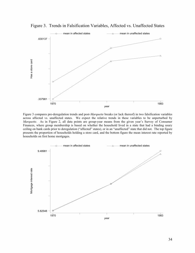
(presumably due to Marquette).12 Figure 3 indicates that variables that should not have been

11 No states made material changes to their usury ceilings between the 1977 SCF survey date and the 1978Marquette decision. 12 The aggregate slowdown in bank card growth evident after 1977 has been attributed to a combination of the early1980s recession and industry growing pains (Mandell 1991).

12

affected by Marquette (these are used in the falsification tests of Section VII) do not in fact

appear to break from trend after 1977. Table 1 shows few observable differences in

demographic characteristics or economic conditions between affected and unaffected states in

1977, but a stark difference in bank card interest rates (which presumably were depressed in

affected states by binding usury ceilings).

The other particularly notable feature of Table 1 is the evident lingering effects of the 1981-

82 recession. Credit card growth, which had surged throughout the 1970s, slowed dramatically

in the late 1970s and early 1980s (see also Figure 1), and unemployment remained high in 1983.

These macroeconomic effects arguably stack the deck against finding effects of usury

deregulation in a statistical sense, since there is probably less variation in card use than there

would have been counterfactually. But the recession should not otherwise contaminate the

results, since the year effects capture time series conditions common to the entire sample, and

household- and state-specific control variables capture local conditions.

Of course, the deeper question to consider regarding the identification issue is why several

states maintained binding usury ceilings as late as the Marquette case while others did not. The

political economy of usury regulation is poorly understood (and the drivers of usury deregulation

even less so), but the fact that the deregulation considered in this paper occurred as the result of a

federal intervention, and a court case at that, mitigates concerns that subsequent behavior in

affected states might be driven by unobserved changes in consumer demand rather than bank

supply. Nevertheless I condition on various household and state characteristics that could be

correlated with both usury law status as of 1977 and changes in demand for credit and various

assets. This strategy is detailed in Section V. Section VII then presents several falsification tests

designed to detect any spurious correlation between deregulation and demand shocks.

13

B. Structural Models

Although (1) captures the structural relationship of interest quite well in the case of interest

rates and card possession, many of the other outcomes (Yist’s) considered in this paper have

additional structural parameters of interest. For example, the structural equation of interest for

bankcard borrowing is:

(2) Bist = a + β1Hist + β2rist + χWist + δs + φt + εist

Where H and r are the endogenous regressors of interest, with H measuring whether

household i has a bankcard, and r measuring the interest rate i faces if it borrows on its

bankcard.13

(2) reveals that estimating (1), the reduced-form, for Bist masks important heterogeneity,

since (1) pools two very different types of cardholders— the marginal ones, for whom new

access to card represents a decrease in the cost of borrowing, and the inframarginal ones, who

likely experience no change (if they live in an unaffected state) or an increase (if they live in an

affected state) in the cost of borrowing. Put differently, to estimate a true interest rate elasticity

of bankcard borrowing, one needs to control for selection into bankcard holding, and therefore

one needs to instrument for both H and r.

This presents a problem. The results in Section V suggest that Xst (the deregulation variable)

can serve as one instrument, but another is required. Ongoing work seeks to develop well-

13 Note that the interest rate should not have an independent effect on demand for card possession (as opposed toborrowing) under standard preferences, since consumers can choose whether to finance balances, and there areseveral other reasons to hold cards (including: the option to borrow, the free float on balances paid in full after onebilling cycle, payment services). If consumers have self-control problems, however, all bets are off. Sophisticatedconsumers with self-control problems might well exhibit an interest rate elasticity of cardholding, since they mayforgo cardholding in order to commit not to borrow at high rates.

14

identified structural models of bankcard borrowing and portfolio choice using additional

instruments.

For now, I rely on an alternative approach to put a bit more structure on the reduced-form

results; namely, adding interactions of household characteristics with the deregulation variable to

(1). With reference to existing evidence on which types of consumers are likely to be liquidity

constrained (e.g., Jappelli 1990), these results will test for heterogeneity in responses across

different types of consumers and help identify the marginal card user (see Section VIII).

V. Impacts of Rate Deregulation on Card Interest Rates & Possession

The next two sections discuss estimates of equation (1) for various outcomes related to credit

card use. The results suggest that deregulation increased both bankcard holding and borrowing.

Robustness and falsification tests in Section VII generally support the interpretation that

deregulation caused these changes by increasing the supply of bankcards.

A. Interest Rates

Table 2 presents estimates of the effect of deregulation on credit card interest rates. The

variables of interest are constructed from SCF questions asking respondents for the interest rate

they pay on bank or store card balances that are not paid in full (i.e., that are carried beyond the

free float period). The SCF does not ask about bankcard rates in particular, so I construct a crude

approximation by limiting the sample to those who report an interest rate, but have only a

bankcard (not a store card). Each row presents results for a different dependent variable, and

each cell contains results on the deregulation variable from a different regression. As such each

column presents results for a different specification, as follows:

15

• column 1 regressions include only the deregulation variable, state and year effects

• column 2 adds variables capturing the race and age of the household head

• column 3 adds household structure, the household head’s education and employment

(including self-employment status), characteristics of the head’s spouse, household income,

housing tenure, and a home mortgage indicator

• column 4 adds the log of aggregate state income, the Gini coefficient on state income, and

the state employment rate.

• column 5 adds interactions of the year dummy and individual covariates, to capture any time-

varying influence of a household’s characteristics on its financial decisions.

The general approach here is to ensure that any observed relationship between deregulation

and the outcomes of interest is not driven somehow by demographic shifts in affected states,

either due to coincidence, or to a political economy story whereby increasing demand in affected

states set in motion the legal process that culminated in the Marquette decision.14 The state

aggregate variables are motivated in part by Glaeser and Scheinkman’s (1998) findings that the

likelihood of a usury ceiling may be increasing with equality and decreasing in income growth,

and in part by the importance of network externalities in bankcard supply (Evans and

Schmalensee, 1999). These factors suggest that card issuer (mass) marketing strategy might

depend on state-level characteristics not entirely captured by the micro data.

The results in Table 2 suggest that deregulation did in fact increase bankcard interest rates.

The approximated annual bankcard rate rises by about 130 basis points in affected states relative

14 Marquette-related proceedings were in fact initiated by a bank in a state with a binding usury ceiling(Minnesota)— in 1976. If a potentially confounding secular increase in demand were driving this proceeding, wemight then expect to see a break from trend in card use before the 1977 SCF, in affected states relative to unaffectedstates. This does not appear to be the case (Figure 2).

16

to unaffected states (this would imply a 9% increase over the 1977 mean of 14.4% in affected

states). Taking the log of the dependent variable yields similar magnitudes, with implied

increases of about 9%. Both the level and log results are consistent across specifications, and all

are statistically significant by a comfortable margin (with t-statistics of 3 or greater). The

combined bank and store card rate increases less, not surprisingly, but still substantially, by

about 90 basis points (implying a 6.4% increase over the 1977 base mean of 14.1% in affected

states). The logged results are insignificant, with slightly larger standard errors than their logged

bankcard rate counterparts, and much smaller point estimates clustered around 0.04. In all, it

seems plausible, at least, that Marquette did in fact increase the interest rate banks charged on

credit card balances held by households in affected states. This finding provides support for

Ausubel’s (1991) “upward-quick” model of credit card interest rates.

B. Card possession

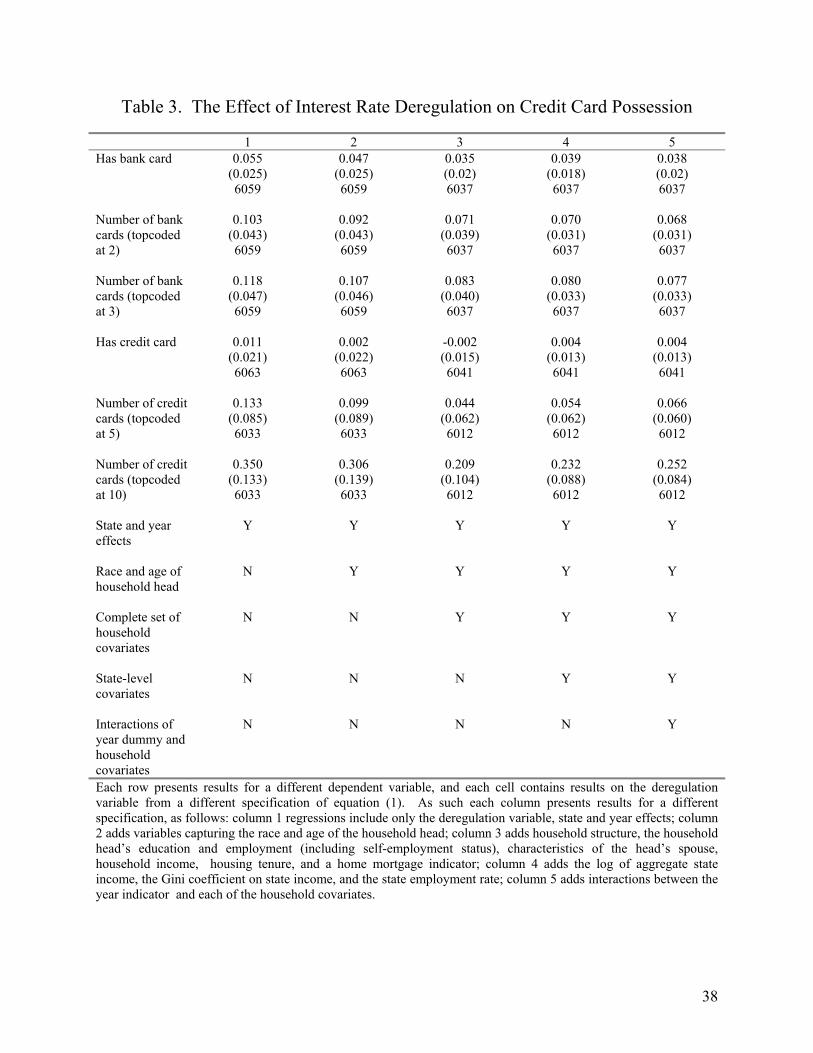
Table 3 presents analogous results for bankcard possession from linear probability estimates

of (1) (probits produced nearly identical results). Possession is arguably the bankcard behavior

of greatest interest, since it is measured with less error than bankcard borrowing (Blanchflower,

Evans, and Oswald), and provides a better summary of the benefits available to cardholders than

actual borrowing. This is because a bankcard provides services that plausibly decrease liquidity

constraints regardless of whether the cardholder actually borrows. These services include

payments, free float, and the option to borrow. The results suggest that the proportion of

households using a bankcard rose between 3.5 and 5.5 percentage points in affected states,

relative to unaffected states, between 1977 and 1983. These are large changes— they would

imply a 10 to 15 percent increase over the base period mean of 0.36 in affected states, and

17

account for 49 to 77 percent of the time series growth in bank card possession in affected states

during this period (Table 1). The estimates are marginally significant, with t-statistics of about 2

in every case. Similar inferences are obtained for the number of bankcards held by a household

(this can be thought of as a proxy for available credit). Row 2 presents results with the

dependent variable topcoded at 2 to reduce the influence of outliers (this censors 2.3% of the

estimation sample), and Row 3 presents results with the number of bankcards topcoded at 3

(censoring 0.7% of the estimation sample). These point estimates imply increases of 0.07 to 0.12

bankcards per household in affected states, or about a 15% increase over the base period means.

This percentage increase is similar to that obtained for card possession, suggesting the much of

the increase in the number of cards may actually be driven by the extensive margin.

The analogous results for all credit cards (where the count does not include gas cards, and

therefore is comprised primarily of bank and store cards) are sensitive to the censoring rule, with

significant increases found when topcoding at 10 cards, but not at 5. The increases of 0.21 to

0.31 of a card found in Row 6 would imply a 9 to 13 percent increase over the base period mean

of 2.4 cards in affected states. There is no evidence of an effect on the extensive margin of

holding any card (Row 4), nor is there a significant effect on holding a store card in particular

(Table 5, Row 1).

The relationship between household characteristics and bank card possession (not reported)

confirm most of the findings of Blanchflower, Evans, and Oswald’s analysis of pooled 1977-

1995 SCF data (which did not include state fixed effects or the deregulation variable).

Conditional on the other observables, white, rich, educated, married, middle-aged, female-

headed, homeowning households with fewer members appear most likely to hold bank cards.

18

C. Summary

In all, the results presented thus far suggest that deregulation did in fact increase both the

number of households holding bank cards, and the number of bank cards in circulation.

Deregulation does not appear to have had a significant effect, however, on overall cardholding.

These results raise the questions of whether bankcards were substitutes for store cards, and/or if

the marginal cardholder produced by deregulation was in fact liquidity constrained. I explore

these questions in the next three sections.

VI. The Impact of Interest Rate Deregulation on Credit Card Borrowing

A. Unconditional Borrowing

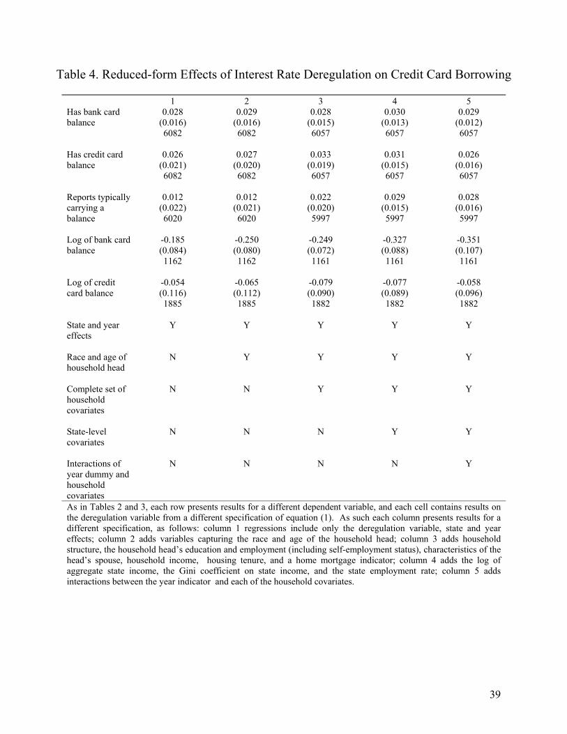
I continue by estimating the reduced-form effect of interest rate deregulation on credit card

borrowing. Table 4, Row 1 presents results for whether a household reported having a bankcard

balance that was incurring finance charges as of the month prior to the SCF survey date. (This

binary parameterization of borrowing is motivated by concerns about outliers and measurement

error.) The estimates suggest a marginally significant, 3 percentage point increase in the number

of households carrying bankcard balances. Taking the point estimates literally, this is a large

increase compared to the estimated 3.5 to 5.5 percentage point possession increases reported in

Table 3. It suggests that at least 55% of the marginal cardholders were borrowing on their

bankcards (the full sample mean in the 1983 SCF is 52%). Of course the true proportion is likely

somewhat higher, since, as Section IV outlines, the reduced-form for unconditional borrowing

captures the net effect of marginal cardholders borrowing more (since one can’t borrow without

a card), and inframarginal cardholders borrowing less (since they now face a higher interest rate).

Row 2 estimates the reduced-form effect on credit card balances generally (this measure is

19

dominated by store and bank cards, and does not include gasoline cards). The results are

virtually identical to those obtained for bank card balances only. This is reassuring-- to the

extent there are changes in overall card borrowing, they should be driven by bank cards (i.e., if

the increase in overall credit card borrowing was significantly larger than for bank card

borrowing, this would arouse suspicion). Row 3 reports results for whether the household

reports that it typically borrows on its bank or store card. The results are generally insignificant,

with somewhat larger standard errors and smaller coefficients than the other measures of

unconditional borrowing (this could well be due to a relatively big underreporting problem with

this variable).

Unfortunately, the 1977 SCF lacks balance data on most other types of borrowing, so it is not

possible to directly calculate the extent to which, if any, new bank card borrowing crowds out

other sources of debt. However, preliminary estimates provide little evidence of crowd-out on

the extensive margin of likely substitutes (revolving credit and installment debt from stores,

consumer loans from banks).

B. Conditional Borrowing

Rows 4 and 5 present estimates for the logarithims of bank and credit card balances,

respectively, and thus condition on borrowing. Although one should not attribute a causal effect

to deregulation in this context, since we know that deregulation also effects that probability that

one borrows, it may be worth noting that the results here appear consistent with a substantial

decrease in borrowing by inframarginal cardholders; i.e., with a nontrivial interest rate elasticity

of borrowing. Alternately, marginal cardholders may borrow less on average than their

predecessors.

20

C. Interpretation

In all, the reduced-form results on credit card borrowing raise two important possibilities.

One is that the marginal cardholder was quite credit constrained; the results on unconditional

borrowing are consistent with very high probabilities of borrowing for marginal bank

cardholders. The second hints that responses to deregulation were heterogeneous, as the results

on unconditional borrowing point to potentially important differences between marginal and

inframarginal cardholders. This further motivates richer models that can distinguish the

mechanisms underlying responses by marginal and inframarginal cardholders. Ongoing work

seeks to develop structural models of the sort described in Section IV. Another approach is to

enhance the reduced-form model. This is undertaken in section VIII.

VII. Falsification Tests

Before exploring heterogeneity in the responses of card use to interest rate deregulation, I

first conduct several falsification tests in an attempt to rule out demand-driven explanations for

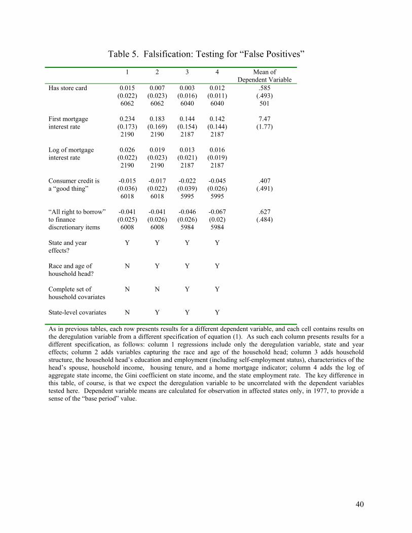
the observed correlations between interest rate deregulation and bank card use. Table 5 presents

the results of falsification tests where I simply replace the dependent variables of equation 1 with

variables that should not be affected by bankcard interest rate deregulation. Finding a “false

positive” here would raise concerns that the “shock” provided by Marquette is actually

correlated with unobserved determinants of demand; i.e., that households in states affected by

Marquette actually had a secular uptick in demand between 1977 and 1983 relative to unaffected

states.

21

The probability of holding a store card should be uncorrelated with bank card deregulation,

since Marquette did not apply to store cards, and since none of the states affected by Marquette

deregulated store card rates between 1977 and 1983. The results in Table 5, row 1 provide no

evidence to the contrary. This is hardly airtight evidence in support of a causal effect of the

deregulation variable on bankcard use, since bank and store cards could be substitutes (or less

likely, complements). Nevertheless one would be concerned if store cards increased along with

the deregulation variable. Row 2 shows no significant effect on first mortgage interest rates.

Rows 3 and 4 display correlations between the deregulation variable and beliefs about the

benefits of consumer credit that are negative, if anything; i.e., the proportion of households

responding that consumer credit is a “good thing”, or that it is “all right to borrow” to finance

discretionary purposes, appears to drop following deregulation.15 It is not yet clear how we

should interpret these results (see the previous footnote), or whether we should take attitudinal

questions seriously at all. But if nothing else these results further alleviate concern that

deregulation might be correlated with unobserved increases in demand.

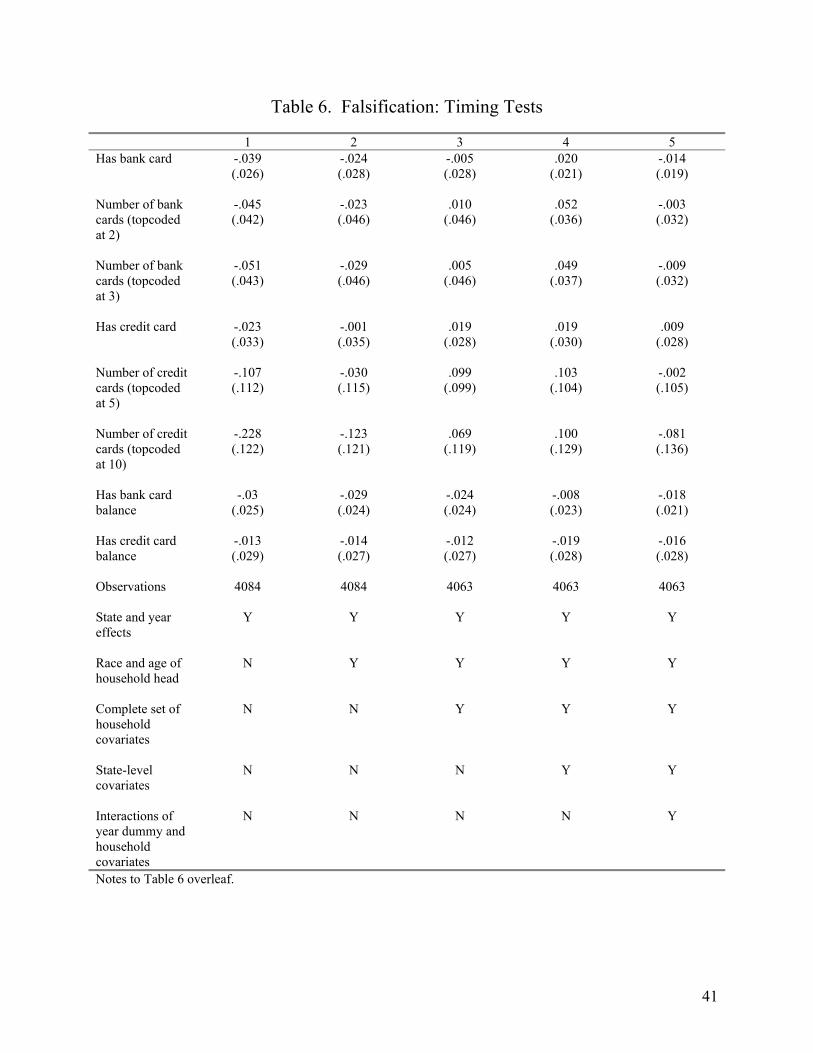
Table 6 presents estimates for a timing falsification model where (1) is estimated on 1970

and 1977 SCF data for the card possession and lending variables of interest (credit card interest

rates are not available in 1970), with deregulation falsely coded as taking effect in 1977 for

households in states that still had binding usury ceilings at that time. This test creates a selection

problem, unfortunately, since many states changed their usury ceilings between 1970 and 1977,

15 These results are intriguing, particularly since the dominant reasons households offer for consumer credit or creditcards being a “bad thing” evoke self-control problems (“encourages impulse buying…. too easy to buy now, paylater….. buy things don’t want or need”, “buy more than you can pay for”). The results hint that there may havebeen some (social) learning about the self-control problems posed by bankcard possession, and that householdsupdated their beliefs about bankcards’ costs and benefits as cards became more prevalent. The results do not appearto be driven by inframarginal cardholders responding to higher interest rate, since “costs too much” is a separate,mutually exclusive response. (Other alternative explanations must be explored, of course; e.g., what if consumergroups targeted consumer credit “awareness” campaigns to affected states in the wake of Marquette?) Future work

22

and I am forced to limit the sample to those states that had stable interest rate regulation during

this period. The results therefore should be interpreted with caution. Estimates are ultimately

based on a sample of households from 27 states (as opposed to the 37 states represented in every

other sample used in this paper), of which only 5 states are labeled as affected (as opposed to 7

elsewhere). The deregulation variable should be uncorrelated with the outcomes of interest in

these tests if deregulation was in fact an exogenous shock to bank card supply. Indeed, there is

virtually no suggestion of a statistically significant relationship in this table. It should be noted,

however, that the standard errors are large enough in most cases to admit the possibility of

correlations that would raise concerns about mean reversion.

VIII. Heterogeneity: In Search of the Marginal Bank Card User

The reduced-form models presented thus far may obscure important heterogeneity in

responses between marginal cardholders (for whom borrowing on bank cards became less

expensive, or at least feasible) and inframarginal cardholders (for whom borrowing might have

become more expensive) in states affected by usury deregulation. In this section I attempt to

identify any important sources of heterogeneity by adding interactions between the deregulation

variable (X) and each of the household control variables (in matrix W) to equation (1). This

increases the main effect on the deregulation variable approximately twofold for the case of

bankcard possession (compare to Table 3, row 1, column 4); however, the standard errors jump

as well (with a p-value of 0.155 for any bank card, and .081 for the number of bank cards). The

interaction terms suggest that marginal cardholders are much more likely to be young (a

whopping 26 percentage point increase in deregulated states relative to the oldest households),

on the nature of consumption responses to increased bankcard use (smooth, or splurge?) will examine these resultsmore closely.

23

have only a high school education (a 9 point increase relative to heads without a high school

education), poor (9 to 13 point increases for the poorest group relative to richer groups), and a

mortgagee.16 Each of these characteristics except for the latter have been widely associated with

liquidity constraints (e.g., Jappelli 1990).

The main effect of deregulation on the proxy for bank card interest rates jumps dramatically

when the interactions are added (coefficient=3.14, standard error=1.49; compare to Table 2, row

1, column 4). Working households with children, male heads, and very little education appear

more likely to face higher rates after deregulation.

Adding the interactions eliminates the main effect of deregulation on binary bankcard

borrowing (coefficent=0.006, standard error=0.045; compare to Table 4, row 1, column 4). Only

young households (compared to the oldest households), married households, and those with

some college education (compared to the least-educated) appear to borrow more, and the effects

are only marginally significant. Conditional borrowing falls dramatically but is imprecisely

estimated (coefficient= -0.89, standard error= 0.70), with the self-employed and those with some

college appearing more likely to borrow.

In all, the large increases in bank cardholding (and, to a lesser extent, on borrowing) among

classes of borrowers widely thought to be liquidity constrained would seem to bode well for

identifying the effects of liquidity on portfolio choice in the next section.

16 Income categories are based on four approximately equal-sized groups in the 1977 data (this approach isnecessitated by the categorical nature of the data). I then deflate the 1983 income variable (which is continuous) to1976 dollars and use the 1977 break points to define the 1983 categories as well.

24

IX. Interest Rate Deregulation and Asset Choice

The results thus far suggest that interest rate deregulation delivered bank cards to a nontrivial

number of households on the margin. Many of these households borrowed actively on their

cards, and many of the marginal cardholders were plausibly credit constrained ex ante. Standard

models of buffer stocks and precautionary saving predict that liquidity constraints force agents to

be sub-optimally liquid and conservative in their asset holdings. Accordingly, this section

presents estimates of reduced-form models that test whether households in states affected by the

deregulation of interest rate ceilings, and in particular those households that appear to be the

marginal cardholders in Section VII, do in fact shift into higher-yielding illiquid and risky assets.

This exercise is hampered somewhat by data limitations in the 1977 SCF, which reports only

categorical values for most asset types. Although the natural variables of interest here are ratios

of asset types to total assets, it is impossible to directly construct these proportions with any

precision in the 1977 SCF.17 Consequently I am forced to parameterize asset holdings as binary

variables, based either on the extensive margin or arbitrary cutoffs. The combination of these

measurement problems and the small net increase in bank cardholding in affected states (3.5 to

5.5 percentage points) dims the prospect of finding significant effects in the basic reduced-form

(equation 1).

I begin by estimating whether deregulation appears to induce households to reduce liquid

asset holdings. There has been a longstanding particular interest in whether credit card use

reduces liquid asset holdings (dating at least to White 1976), motivated primarily by the question

of whether the payments feature of credit cards reduces the transactions demand for money (see

also Duca and Whitsell 1995, and Blanchflower, Evans, and Oswald). Of course credit cards

17 The next draft will include asset share estimates based in part on 1977 holdings that are predicted from a modelestimated on 1970 data, conditional on the asset interval (which is observed in both years).

25

might reduce liquid asset holdings through another channel as well— if they relax liquidity

constraints and thereby reduce the need to hold buffer stocks (which must be kept relatively

liquid for emergencies). Table 7, Rows 1-3 present the reduced-form estimates for checking

account balances (row 1), savings account balances (row 2), and a binary variable for savings

account ownership (row 3). The model delivers the expected signs for the savings account

variables but not for checking balances, and the standard errors are too large to identify the

plausibly small effects one would expect on these binary outcomes. I encounter a similar

problem with illiquid assets (certificates of deposit and government savings bonds) and a risky

asset (stocks). Results are presented for the extensive margin in each case, but binary variables

based on the various categorical cutoffs posed by the 1977 survey fared no better.

The basic reduced-form model accordingly provides little leverage for testing the prediction

that interest rate deregulation should induce portfolio shifts (via relaxation of liquidity

constraints). Part of the power problem stems from the fact that, as in the case of borrowing, the

reduced-form model may obscure countervailing effects on marginal and inframarginal

cardholders in affected states. In contrast, the large effects on cardholding and borrowing for

certain, plausibly credit-constrained groups (Section VII) suggest that the enhanced reduced-

form model with interactions holds some promise for identifying effects of deregulation (and

bank card use) on asset choice.18

Indeed, adding the interaction terms to the equations for asset holdings yields some

significant results— and little support for the prediction that marginal, liquidity-constrained

households should adjust their portfolios in favor of more illiquid, risky assets upon accessing

18 The limitations of the reduced-form again motivate structural approaches. Ongoing work suggests that certainstructural parameters should appear in asset choice models that are absent from the borrowing model. For example,it would be useful to distinguish the impact of the option value of borrowing on portfolio choice from the impact ofactual borrowing (or convenience use).

26

credit. The youngest households in affected states do appear to become much more likely to

hold a government savings bond and less likely to have savings account (relative to the oldest

households) after deregulation, which jibes with the canonical predictions. However they seem

far less likely to hold stock or be self-employed, findings that are at odds with the canonical

predictions. The poorest households appear to become more likely to be self-employed or to

hold a government savings bond, certificate of deposit, or stock than their richer counterparts,

but they also seem to increase their liquid asset holdings (this is a case where it would be

particularly useful to have data on the ratios of each of these different types of assets to total

assets). There does not appear to be significant variation in portfolio choice by education level

in deregulated states, in contrast to bank card usage results. Males seem to begin holding more

assets in their savings accounts, and are less likely to be self-employed (these could be

inframarginal effects of males facing the higher interest rates observed in Section VII). Working

households become more likely to hold both stock and liquid assets. Married households

become more likely to hold a CD and substantial amounts of stock, but also more likely to hold

high checking account balances after deregulation. Blacks appear to enter self-employment and

hold larger savings account balances, despite no observable changes in card use.

Although measurement issues discourage drawing firm conclusions from the results in this

section, it nevertheless seems fair to say that the findings here do not jibe easily with standard

models of liquidity constraints.

27

X. Summary and Implications

This paper develops a new type of evidence on the impacts of liquidity on consumer

behavior. The results suggest that binding interest rate ceilings in several states during the late

1970s kept perhaps 4 or 5 out of every 100 households in these states from obtaining bank credit

cards, and that at least 55% of these households borrowed on bank credit cards when given the

opportunity. Moreover these marginal households were probably even less likely to consume out

of liquidity than the 57% of households that remained without bank credit cards in the 1983 SCF

(Jappelli, Pischke, and Souleles 1998). The results here are thus consistent with a clear majority

of U.S. households having a nonzero marginal propensity to consume (MPC) out of liquidity.

The fact that it is possible to identify borrowing increases at all in data reported by consumers

(who are notorious for understating their credit card borrowing) suggests that these MPCs could

be substantial, as in Gross and Souleles (2002).

But an MPC to consume out of liquidity is not a sufficient condition for establishing the

existence or importance of liquidity constraints. A stricter test for the presence of liquidity

constraints is whether consumers respond to increased liquidity by shifting into illiquid, riskier

assets. The results in this paper offer no evidence that they do, despite the fact that the marginal

cardholder appears to be young, poor, and relatively poorly educated— all characteristics

commonly associated with facing binding liquidity constraints. In other words, a substantial

number of households that appeared to be credit constrained suddenly obtained access to

liquidity as the result of interest rate deregulation, and they did not adjust their portfolios as

standard models of liquidity constraints would predict. Data limitations prevent drawing firm

conclusions, but the results are suggestive and motivate consideration of alternative explanations.

28

One type of alternative (or complementary) model postulates that consumers face what might

be termed “commitment constraints”. The possibility that some consumers are prone to splurge,

with potentially adverse consequences, in the absence of effective commitment devices is

gaining currency.19 Recent simulations, for example, have shown that preferences which allow

for self-control problems explain household balance sheets much better than standard

preferences (Angeletos, et. al. 2001; Laibson, Repetto, and Tobacman forthcoming).

Far more work can be done to study the impact of liquidity, and or any lack thereof, in

consumer credit markets. One offshoot of this paper is estimating the impact of Marquette-

induced liquidity on the level, composition, and time-path of consumption— do households

smooth or splurge when they obtain a credit card?— and will proceed to estimate any long-run

impacts on savings rates and savings adequacy. This new work should light on the nature and

magnitude of excess sensitivity, and on the structure of consumer preferences and high-

frequency intertemporal choice.

19 Zinman (2003) explores whether the explosive growth of debit card use over the last decade is due (in part) todebit use serving as a commitment device against “overborrowing” on credit cards.

29

References

American Bankers’ Association, “Summary of State Banking Legislation”, various years.

Athreya, Kartik, “The Growth of Unsecured Credit: Are We Better Off?”, Federal Reserve Bank ofRichmond Economic Quarterly, 87/3 (2001), 11.

Angeletos, George-Marios, Laibson, David I., Repetto, Andrea, Tobacman, Jeremy, and Weinberg,Stephen, “The Hyperbolic Buffer Stock Model: Calibration, Simulation, and Empirical Evaluation”,Journal of Economic Perspectives, 15/3(Summer 2001), 47-68.

Ausubel, Lawrence M., “The Failure of Competition in the Credit Card Market”, American EconomicReview, 81(1991), 50-81.

Ausubel, Lawrence M., “Adverse Selection in the Credit Card Market”, mimeo, June 17, 1999.

Bertaut, Carol C., and Haliassos, Michael, “Debt Revolvers for Self-Control”, mimeo, June 10, 2002.

Blanchflower, David G., Evans, David S., Oswald, Andrew J., “Credit Cards and Consumers”, NationalEconomic Research Associates Working Paper (undated).

Blitz, Rudolph C., and Long, Millard F., “The Economics of Usury Regulation”, Journal of PoliticalEconomy, 73/6(1965), 608.

Board of Governors of the Federal Reserve System, Statistical Release G.19, July 2002.

Browning, Martin, and Lusardi, Annamaria, “Household Saving: Micro Theories and Macro Facts”,Journal of Economic Literature, 34(1996), 1797-1855.

Canner, Glenn B., and Fergus, James T., “The Effects on Consumers and Creditors of Proposed Ceilingson Credit Card Interest Rates”, Federal Reserve Bulletin, 73/10(October 1987), 783.

DellaVigna, Stefano, and Malmendier, Ulrike, “Contract Design and Self-Control: Theory andEvidence”, mimeo, December 3, 2001.

Duca, J. V., and Whitsell, W. C., “Credit Cards and Money Demand: A Cross-Sectional Study”, Journalof Money, Credit, and Banking, 27(1995), 604-623.

Dunkelberg, William, et. al. “CRC 1979 Consumer Financial Survey”, Monograph 22 (PurdueUniversity, Krannert Graduate School of Management, Credit Research Center), 1981

Evans, David S., and Leder, Matthew R., “The Role of Credit Cards in Providing Financing for SmallBusinesses”, National Economic Research Associates Working Paper (undated).

Evans, David S., and Schmalensee, Richard, Paying with Plastic: The Digital Revolution in Buying andBorrowing (MIT Press: Cambridge, MA), 1999.

Glaeser, Edward L., and Scheinkman, Jose, “Neither a Borrower Nor a Lender Be: An EconomicAnalysis of Interest Restrictions and Usury Laws”, Journal of Law and Economics, XLI(1998), 1.

30

Goldberg, Lawrence G., “The Effect of State Banking Regulations on Bank Credit Card Use: Comment”,Journal of Money, Credit, and Banking, 7/1(1975), 105.

Gross, David B., and Souleles Nicholas S., “Do Liquidity Constraints and Interest Rates Matter forConsumer Behavior? Evidence from Credit Card Data”, Quarterly Journal of Economics, 117/1(2002),149-177.

Guiso, Luigi, Jappelli, Tullio, Terlizzese, Daniele, “Income Risk, Borrowing Constraints, and PortfolioChoice”, American Economic Review, 86/1(1996), 158-72.

Gushee, Charles, ed., The Cost of Personal Borrowing (Basic Books: Boston), various years.

Hubbard, R. Glenn, and Judd, Kenneth, “Liquidity Constraints, Fiscal Policy, and Consumption”,Brookings Papers on Economic Activity, 1(1986), 1-59.

Hurst, Erik, and Lusardi, Annamaria, “Liquidity Constraints, Wealth Accumulation, andEntrepreneurship”, mimeo, March 2002.

Jappelli, Tulio, “Who is Credit Constrained in the U.S. Economy”, Quarterly Journal of Economics,February 1990, v. 105, iss. 1, pp. 219-34.

Jappelli, Tulio, and Pagano, Marco, “The Welfare Effects of Liquidity Constraints”, Oxford EconomicPapers, 51(1999), 410-430.

Jappelli, Tulio, Pischke, Stephen, and Souleles, Nicholas, “Testing for Liquidity Constraints in EulerEquations with Complementary Data Sources”, Review of Economics and Statistics, LXXX(1998), 251-262.

Kennickell, Arthur B., Starr-McCluer, Martha, and Surette, Brian J., “Recent Changes in U.S. FamilyFinances: Results from the 1998 Survey of Consumer Finances”, Federal Reserve Bulletin, vol. 86(January 2000), pp. 1-29.

Laibson, David I., “Golden Eggs and Hyperbolic Discounting”, Quarterly Journal of Economics,112/2(1997), 443.

Laibson, David I., Repetto, Andrea, and Tobacman, Jeremy, “Self-Control and Saving for Retirement”,Brookings Papers on Economic Activity, Vol. 1998/1 (1998), 91.

Laibson, David I., Repetto, Andrea, and Tobacman, Jeremy, “A Debt Puzzle”, in eds. Aghion, Phillipe,Frydman, Roman, Stiglitz, Joseph, and Woodford, Michael, Knowledge, Information, and Expectations inModern Economics: In Honor of Edmund S. Phelps, forthcoming.

Mandell, Lewis, The Credit Card Industry: A History (Twayne: Boston, MA), 1990.

O’Donoghue, Ted D., and Rabin, Matthew, “Choice and Procrastination”, Quarterly Journal ofEconomics, 116/1(February 2001), 121-160.

White, K. J., “The Effect of Bank Credit Cards on the Household Transactions Demand for Money”,Journal of Money, Credit, and Banking, 8(1976), 51.

31

Figure 1. Revolving Credit Per Capita (2001 Dollars)

0

500

1000

1500

2000

2500

1968 1973 1978 1983 1988 1993 1998

2001

Dol

lars

Source: Series G-19, Board of Governors of the Federal Reserve System

Figure 2. Trends in Bank Card Use, Affected vs. Unaffected StatesH

as a

ban

k ca

rd

year

mean in affected states mean in unaffected states

1968 1983

.073797

.434247

Figure 2 compares pre-deregulation trends and post-Marquette breaks in bank card use across affected vs.unaffected states. All data points are group-year means from the given year’s Survey of Consumer Finances, wheregroup membership is based on whether the household lived in a state that had a binding usury ceiling on bank cardsprior to deregulation (“affected” states), or in an “unaffected” state that did not. The top figure presents theproportion of households holding a bank card, the middle figure the mean number of bank cards held by households,and the bottom figure the proportion of households that reported carrying a balance (paying interest) on a bank cardin the month prior to the survey date.

.

Num

ber o

f ban

k ca

rds

year

mean in affected states mean in unaffected states

1970 1983

.178197

.616438

33

Figure 2, continuedH

as b

ank

card

bal

ance

year

mean in affected states mean in unaffected states

1970 1983

.044025

.232877

34

Figure 3. Trends in Falsification Variables, Affected vs. Unaffected StatesH

as a

sto

re c

ard

year

mean in affected states mean in unaffected states

1970 1983

.337981

.630137

Figure 3 compares pre-deregulation trends and post-Marquette breaks (or lack thereof) in two falsification variablesacross affected vs. unaffected states. We expect the relative trends in these variables to be unperturbed byMarquette. As in Figure 2, all data points are group-year means from the given year’s Survey of ConsumerFinances, where group membership is based on whether the household lived in a state that had a binding usuryceiling on bank cards prior to deregulation (“affected” states), or in an “unaffected” state that did not. The top figurepresents the proportion of households holding a store card, and the bottom figure the mean interest rate reported byhouseholds on first home mortgages.

Mor

tgag

e in

tere

st ra

te

year

mean in affected states mean in unaffected states

1970 1983

5.82548

9.48981

Table 1. Summary Statistics, Selected Variables from the 1977 & 1983 SCFs

Variable1977 1983 1977

affected1977

unaffected1983

affected1983

unaffectedAny bank card

.376(.485)

.412(.492)

.363(.481)

.380(.486)

.434(.496)

.407(.491)

Number of bank cards

.515(.726)

.568(.746)

.493(.715)

.521(.729)

.616(.776)

.556(.738)

Paying interest on bank card

.155(.361)

.215(.411)

.153(.360)

.155(.362)

.233(.422)

.211(.408)

Interest rateon bank card

16.4(3.4)

17.9(3.0)

14.4(3.8)

17.0(3.1)

17.0(3.2)

18.1(2.9)

Interest rate on credit card

16.2(3.6)

17.6(3.5)

14.1(3.7)

16.8(3.4)

16.2(4.1)

17.9(3.3)

Any credit card

.597(.491)

..627(.484)

.643(.479)

.585(.493)

.682(.466)

.613(.487)

Any savings account

.784(.411)

.611(.487)

.826(.380)

.773(.419)

.633(.482)

.606(.489)

Any CD .138(.346)

.197(.398)

.145(.353)

.137(.343)

.226(.419)

.190(.393)

Any stock .255(.436)

.286(.452)

.279(.449)

.248(.432)

.301(.459)

.282(.450)

Male head .775(.418)

.738(.440)

.762(.426)

.779(.415)

.742(.438)

.737(.440)

High school educated or less

.323(.470)

.291(.454)

.298(.458)

.338(.473)

.273(.446)

.295(.456)

Unemployed head

.029(.168)

.075(.263)

.038(.191)

.027(.161)

.060(.238)

.079(.269)

Wife works .327(.469)

.321(.467)

.355(.479)

.320(.467)

.335(.472)

.317(.465)

Age of head 46.9(17.3)

46.6(17.3)

47.0(17.5)

46.9(17.2)

46.8(17.1)

46.5(17.4)

Less than $7500 income ($1976)

.223(.416)

.325(.469)

.208(.407)

.227(.419)

.316(.465)

.327(.469)

Gini coefficienton income, state

.399(.019)

.409(.017)

.401(.022)

.399(.018)

.403(.015)

.410(.017)

Employment rate, state

.463(.026)

.487(.036)

.454(.023)

.465(.026)

.480(.034)

.489(.036)

N 2417 3665 504 1913 730 2935

36

Notes to Table 1.

Cells present (sub-)sample means, with standard deviations in parentheses. Selected cells include the number ofnonmissing observations; 1983 variables have few if any missing observations due to imputations by FederalReserve Board staff. Bank card interest rates are observed only for those households with a bank card but not storecard. “Affected” households are those living in states that had binding usury ceilings on bank credit card interestrates as of the 1977 SCF. “Unaffected” households are those living in states that did not have binding usury ceilingsas of the 1977 SCF. The last row gives the number of observations in the full (sub-)sample (I exclude the highincome oversample from the 1983 data, and observations from Oregon or with unknown state of residence from the1977 data).

37

Table 2. The Effect of Interest Rate Deregulation on Credit Card Interest Rates

1 2 3 4 5Bank cardinterest rate

1.39(0.37)1936

1.34(0.39)1936

1.36(0.40)1933

1.25(0.35)1933

1.18(0.36)1933

Log of bank cardinterest rate

0.099(0.027)1936

0.093(0.029)1936

0.094(0.03)1933

0.084(0.028)1933

0.077(0.028)1933

Bank or storecard interest rate

0.969(0.451)2755

0.884(0.454)2755

0.944(0.452)2750

0.893(0.5)2750

0.845(0.485)2750

Log of bank orstore cardinterest rate

0.042(0.037)2755

0.034(0.037)2755

0.041(0.037)2750

0.038(0.043)2750

0.034(0.042)2750

State and yeareffects

Y Y Y Y Y

Race and age ofhousehold head

N Y Y Y Y

Complete set ofhouseholdcovariates

N N Y Y Y

State-levelcovariates

N N N Y Y

Interactions ofyear dummy andhouseholdcovariates

N N N N Y

Each row presents results for a different dependent variable, and each cell contains results on the deregulationvariable from a different specification of equation (1). As such each column presents results for a differentspecification, as follows: column 1 regressions include only the deregulation variable, state and year effects; column2 adds variables capturing the race and age of the household head; column 3 adds household structure, the householdhead’s education and employment (including self-employment status), characteristics of the head’s spouse,household income, housing tenure, and a home mortgage indicator; column 4 adds the log of aggregate stateincome, the Gini coefficient on state income, and the state employment rate; column 5 adds interactions between theyear indicator and each of the household covariates.

38

Table 3. The Effect of Interest Rate Deregulation on Credit Card Possession

1 2 3 4 5Has bank card 0.055

(0.025)6059

0.047(0.025)6059

0.035(0.02)6037

0.039(0.018)6037

0.038(0.02)6037

Number of bankcards (topcodedat 2)

0.103(0.043)6059

0.092(0.043)6059

0.071(0.039)6037

0.070(0.031)6037

0.068(0.031)6037

Number of bankcards (topcodedat 3)

0.118(0.047)6059

0.107(0.046)6059

0.083(0.040)6037

0.080(0.033)6037

0.077(0.033)6037

Has credit card 0.011(0.021)6063

0.002(0.022)6063

-0.002(0.015)6041

0.004(0.013)6041

0.004(0.013)6041

Number of creditcards (topcodedat 5)

0.133(0.085)6033

0.099(0.089)6033

0.044(0.062)6012

0.054(0.062)6012

0.066(0.060)6012

Number of creditcards (topcodedat 10)

0.350(0.133)6033

0.306(0.139)6033

0.209(0.104)6012

0.232(0.088)6012

0.252(0.084)6012

State and yeareffects

Y Y Y Y Y

Race and age ofhousehold head

N Y Y Y Y

Complete set ofhouseholdcovariates

N N Y Y Y

State-levelcovariates

N N N Y Y

Interactions ofyear dummy andhouseholdcovariates

N N N N Y

Each row presents results for a different dependent variable, and each cell contains results on the deregulationvariable from a different specification of equation (1). As such each column presents results for a differentspecification, as follows: column 1 regressions include only the deregulation variable, state and year effects; column2 adds variables capturing the race and age of the household head; column 3 adds household structure, the householdhead’s education and employment (including self-employment status), characteristics of the head’s spouse,household income, housing tenure, and a home mortgage indicator; column 4 adds the log of aggregate stateincome, the Gini coefficient on state income, and the state employment rate; column 5 adds interactions between theyear indicator and each of the household covariates.

39

Table 4. Reduced-form Effects of Interest Rate Deregulation on Credit Card Borrowing

1 2 3 4 5Has bank cardbalance

0.028(0.016)6082

0.029(0.016)6082

0.028(0.015)6057

0.030(0.013)6057

0.029(0.012)6057

Has credit cardbalance

0.026(0.021)6082

0.027(0.020)6082

0.033(0.019)6057

0.031(0.015)6057

0.026(0.016)6057

Reports typicallycarrying abalance

0.012(0.022)6020

0.012(0.021)6020

0.022(0.020)5997

0.029(0.015)5997

0.028(0.016)5997

Log of bank cardbalance

-0.185(0.084)1162

-0.250(0.080)1162

-0.249(0.072)1161

-0.327(0.088)1161

-0.351(0.107)1161

Log of creditcard balance

-0.054(0.116)1885

-0.065(0.112)1885

-0.079(0.090)1882

-0.077(0.089)1882

-0.058(0.096)1882

State and yeareffects

Y Y Y Y Y

Race and age ofhousehold head

N Y Y Y Y

Complete set ofhouseholdcovariates

N N Y Y Y

State-levelcovariates

N N N Y Y

Interactions ofyear dummy andhouseholdcovariates

N N N N Y

As in Tables 2 and 3, each row presents results for a different dependent variable, and each cell contains results onthe deregulation variable from a different specification of equation (1). As such each column presents results for adifferent specification, as follows: column 1 regressions include only the deregulation variable, state and yeareffects; column 2 adds variables capturing the race and age of the household head; column 3 adds householdstructure, the household head’s education and employment (including self-employment status), characteristics of thehead’s spouse, household income, housing tenure, and a home mortgage indicator; column 4 adds the log ofaggregate state income, the Gini coefficient on state income, and the state employment rate; column 5 addsinteractions between the year indicator and each of the household covariates.

40

Table 5. Falsification: Testing for “False Positives”

1 2 3 4 Mean ofDependent Variable

Has store card 0.015(0.022)6062

0.007(0.023)6062

0.003(0.016)6040

0.012(0.011)6040

.585(.493)501

First mortgageinterest rate

0.234(0.173)2190

0.183(0.169)2190

0.144(0.154)2187

0.142(0.144)2187

7.47(1.77)

Log of mortgage interest rate

0.026(0.022)2190

0.019(0.023)2190

0.013(0.021)2187

0.016(0.019)2187

Consumer credit is a “good thing”

-0.015(0.036)6018

-0.017(0.022)6018

-0.022(0.039)5995

-0.045(0.026)5995

.407(.491)

“All right to borrow”to finance discretionary items

-0.041(0.025)6008

-0.041(0.026)6008

-0.046(0.026)5984

-0.067(0.02)5984

.627(.484)

State and yeareffects?

Y Y Y Y

Race and age ofhousehold head?

N Y Y Y

Complete set ofhousehold covariates

N N Y Y

State-level covariates N Y Y Y

As in previous tables, each row presents results for a different dependent variable, and each cell contains results onthe deregulation variable from a different specification of equation (1). As such each column presents results for adifferent specification, as follows: column 1 regressions include only the deregulation variable, state and yeareffects; column 2 adds variables capturing the race and age of the household head; column 3 adds householdstructure, the household head’s education and employment (including self-employment status), characteristics of thehead’s spouse, household income, housing tenure, and a home mortgage indicator; column 4 adds the log ofaggregate state income, the Gini coefficient on state income, and the state employment rate. The key difference inthis table, of course, is that we expect the deregulation variable to be uncorrelated with the dependent variablestested here. Dependent variable means are calculated for observation in affected states only, in 1977, to provide asense of the “base period” value.

41

Table 6. Falsification: Timing Tests

1 2 3 4 5Has bank card -.039

(.026)-.024(.028)

-.005(.028)

.020(.021)

-.014(.019)

Number of bankcards (topcodedat 2)

-.045(.042)

-.023(.046)

.010(.046)

.052(.036)

-.003(.032)

Number of bankcards (topcodedat 3)

-.051(.043)

-.029(.046)

.005(.046)

.049(.037)

-.009(.032)

Has credit card -.023(.033)

-.001(.035)

.019(.028)

.019(.030)

.009(.028)

Number of creditcards (topcodedat 5)

-.107(.112)

-.030(.115)

.099(.099)

.103(.104)

-.002(.105)

Number of creditcards (topcodedat 10)

-.228(.122)

-.123(.121)

.069(.119)

.100(.129)

-.081(.136)

Has bank cardbalance

-.03(.025)

-.029(.024)

-.024(.024)

-.008(.023)

-.018(.021)

Has credit cardbalance

-.013(.029)

-.014(.027)

-.012(.027)

-.019(.028)

-.016(.028)

Observations 4084 4084 4063 4063 4063

State and yeareffects

Y Y Y Y Y

Race and age ofhousehold head

N Y Y Y Y

Complete set ofhouseholdcovariates

N N Y Y Y

State-levelcovariates

N N N Y Y

Interactions ofyear dummy andhouseholdcovariates

N N N N Y

Notes to Table 6 overleaf.

42

Notes to Table 6.

Results are presented for estimates of equation (1), the basic reduced-form model, using 1970 and 1977 data, withhouseholds in states that still faced binding usury ceilings in 1977 falsely labeled as having deregulated. Wetherefore expect the deregulation variable here to be uncorrelated with card usage. Sample sizes are lower than forprevious estimates due to the elimination of 10 states that made material changes to their bank card interest rateusury laws between 1970 and 1977. As in previous tables, each row presents results for a different dependentvariable, and each cell contains results on the deregulation variable from a different specification of equation (1).As such each column presents results for a different specification, as follows: column 1 regressions include only thederegulation variable, state and year effects; column 2 adds variables capturing the race and age of the householdhead; column 3 adds household structure, the household head’s education and employment (including self-employment status), characteristics of the head’s spouse, household income, housing tenure, and a home mortgageindicator; column 4 adds the log of aggregate state income, the Gini coefficient on state income, and the stateemployment rate.

43

Table 7. Reduced-form Effects of Interest Rate Deregulation on Asset Choice

1 2 3 4Checking accountbalances above 1977median

0.032(0.028)5775

0.023(0.031)5775

0.009(0.026)5764

0.014(0.025)5764

Savings accountbalances above 1977median

-0.033(0.026)5683

-0.037(0.025)5683

-0.041(0.024)5672

-0.053(0.022)5672

Has savings account -0.019(0.024)6027

-0.025(0.025)6027

-0.021(0.021)6012

-0.007(0.019)6012

Has governmentsavings bond

0.025(0.02)6025

0.019(0.02)6025

0.016(0.021)6007

-0.005(0.019)6007

Has certificate ofdeposit

0.024(0.017)6017

0.026(0.017)6017

0.019(0.017)5999

0.020(0.017)5999

State and yeareffects?

Y Y Y Y

Race and age ofhousehold head?

N Y Y Y

Complete set ofhousehold covariates

N N Y Y

State-levelcovariates

N N N Y

As in Tables 2, 3, 5, and 6, each row presents results for a different dependent variable, and each cell containsresults on the deregulation variable from a different specification of equation (1). As such each column presentsresults for a different specification, as follows: column 1 regressions include only the deregulation variable, stateand year effects; column 2 adds variables capturing the race and age of the household head; column 3 addshousehold structure, the household head’s education and employment (including self-employment status),characteristics of the head’s spouse, household income, housing tenure, and a home mortgage indicator; column 4adds the log of aggregate state income, the Gini coefficient on state income, and the state employment rate.